Operations research
2 likes1,699 views

This document provides an overview of the history and objectives of operations research. It discusses how operations research originated during World War II to help optimize the use of limited military resources. After the war, operations research techniques were applied to industrial problems to maximize profits and minimize costs. The document outlines the key objectives of operations research as providing a scientific basis for management decision making and helping managers make better decisions through the use of mathematical modeling and analysis.


![Inventory Control 377377377377377
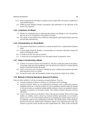
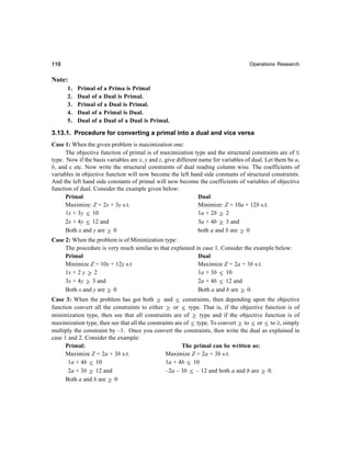
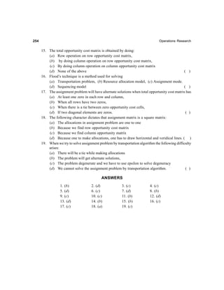
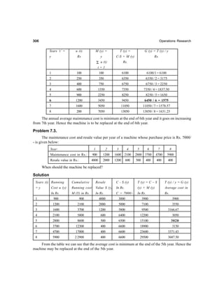
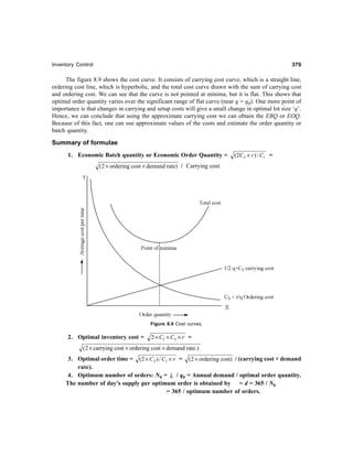
By trial and error method we have seen that economic quantity exists at a point where both
ordering cost and inventory carrying cost are equal. This is the basis of algebraic method of derivation
of formula.The figure 8.8 shows the lot size ‘q’, uniform demand ‘r’ and the pattern of inventory
cycle.
Figure 8.8. Deterministic uniform demand with no shortages.
Total inventory in one cycle i.e. for one unit of time = Area or triangle OAB = ½ the base (t) ×
altitude (q) =
½ × q × t = ½ qt
{This can also be done mathematically by using calculus. At any time ‘t’ from the
beginning of the cycle (where ‘t’ does not represent the time of one cycle), the
inventory = (q – rt). Hence the total inventory in the small time interval t to (t + tδ )
is q- rt) × tδ . Summing over the period ‘t’ of one cycle, the total inventory in one
cycle is:
= ∫ −==−
t
rtqtdtrtq
0
2
2/)( ][ = rttqtrtqt ×−=− ½]½[ 2
= As we know q = rt, we can write as qt – ½ qt = ½ qt.}
Carrying cost for ‘t’ units of time = ½ qt × C1
Set up cost for one cycle is C3
Hence total cost for one unit of time = carrying cost + ordering cost = ½ qt C1 + C3
Total cost per unit of time = Cq = {½ qtC1 + C3} / t = ½ q C1 + C3/t
(We know that q = rt hence t = q/r), substituting this for t in the above equation, we get
Cq = ½ q C1 + C3r/q - this is known as COST EQUATION.
(Note: For any inventory model, first we have to get this cost equation and then we have to
optimize)](https://image.slidesharecdn.com/operationsresearch-151024043006-lva1-app6892/85/Operations-research-388-320.jpg)


![Inventory Control 391391391391391
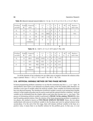
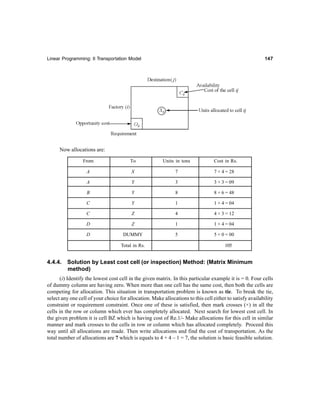
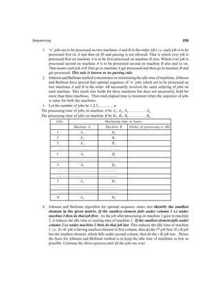
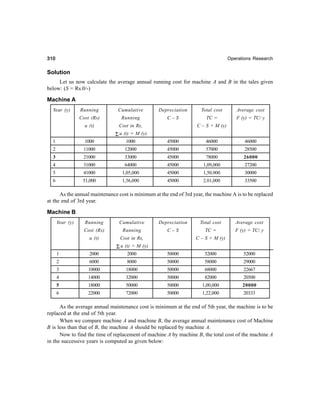
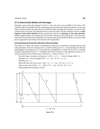
Figure. 8.11.
In the figure, we can see that in the first time period t1 inventory build up, as the demand rate is
less than the production rate (r < k), i.e. the constant rate of replenishment is (k – r). In the second
period t2 items are consumed at the demand rate ‘r’. If we workout the total cost of inventory per unit
of time as usual, we get:
Cq = (q / 2) { (k – r ) / k } C1 + C3 (r/q) By equating the first derivative to zero, we get,
dCq / dq = (C1 / 2) ( 1 – r/k) – (C3 r / q2) = 0 which will give
q0 = )/2( 13 CC × {r / 1 – (r/k)} OR q0 = )//( rkk × rC32 / C1
t0 = q0 / r = 32C / { rC1 ( 1 – r/k)} OR t0 = )/( rkk − × 32C / C1r
C0 = 132 CC (r / 1 – r/k). OR C0 = )( rk − / k × rCC 312
Points to Remember
(a) The carrying cost per unit of time is reduced from cost of first model by a ratio of
[1 – (r / k).] But set up cost remains same.
(b) If we substitute a value of infinity to k in the model shown above, we will get the
results of the first model.
(c) If the production rate is very low, then the lot size should be taken large, because
much of the production will be consumed during the production period and hence the
inventory in the second part of the graph will be built at a very low rate.
(d) If r > k then there will be no inventory.
Problem 8.23
An item is produced at the rate of 50 items per day. The demand occurs at the rate of 25 units per
day. If the set up cost is Rs. 100/- per run and holding cost is Rs.0.01 per unit of item per day, find the
economic lot size for one run, assuming that the shortages are not permitted.](https://image.slidesharecdn.com/operationsresearch-151024043006-lva1-app6892/85/Operations-research-402-320.jpg)


![396396396396396 Operations Research
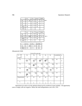
q0 = r t0 = )}/)(2{( 21213 CCCCrC + (Attention is to be given to see that the EOQ model is
multiplied by a factor (C1 + C2) / C2
OR q0 = )( 21 CC + / C2 × λ32( C / C1)
t0 = q0 /r = )}(2{ 213 CCC + / C1 r C2 (Here also the optimal time formula is multiplied by
(C1 + C2) / C2
OR t0 = q0 / λ = )21 CC + / C2 × )/2( 13 λCC
C0 = )/(( 212 CCC + × )2( 31 λCC
Imax = Maximum inventory = S0 = [C2 / (C1 + C2)] × q0 = )]/([ 212 CCC + × )/2( 13 CC λ
S0 = )}(/)2{( 21123 CCCCrC + this is also known as Order level model.
z0 = q0 – S0 = )(/)2{( 21213 CCCCrC +×
(Note: By keeping C2 = ∞ , the above model reduces the deterministic demand EOQ model).
Problem 8.30.
The demand for an item is uniform at the rate of 25 units per month. The set up cost is Rs. 15/-
per run. The production cost is Re.1/- per item and the inventory-carrying cost is Rs. 0. 30 per item per
month. If the shortage cost is Rs. 1.50 per item per month, determine how often to make a production
run and what size it should be?
Solution
Data: r = 25 units per month, C3 = Rs.15/- per run, b = Re. 1/- C1 Rs. 0.30 per item per month,
C2 = Rs. 1.50 per item per month. Where b = production cost, hence Set up cost is to be taken as C3
+ bq. In this example it will become Rs. 15./- + Re. 1/- = Rs.16/-. This will be considered when
working the total cost of inventory and not the economic order quantity, as the any increase in C3 will
not have effect on q0.
Remember when any thing is added to the setup cost, the optimal order quantity will not
change.
q0 = )}(2{ 213 CCrC + / (C1 C2) = )80.125152{( ××× / ( 0.30 x 1.50)} = 10 30 = 54
items. And optimal time = q0 / r = 54 / 25 = 2.16 months.
Optimal cost = C(S, t) = (1/t) × [ (C1S2 / 2r) + C2 (tr – S2) / 2r] + [(C3/t) + br] because (q / t) = r
Problem 8.31.
A particular item has a demand of 9,000 units per year. The cost of one procurement is Rs. 100/-
and the holding cost per unit is Rs. 2.40 per year. The shortages are allowed are the shortage cost
Rs. 5/- per unit per year. (a) Find Economic lot size, (b) Number of orders per year, (c) The time
between two orders, and
(d) Total cost per year including material cost, taking unit price as Re.1/- per unit.
Solution
Data: λ = 9,000 units per year, C1 = Rs. 2.40 per unit per year, C2 = Rs. 5/- per unit per year, C3
Rs. 100/- per procurement.](https://image.slidesharecdn.com/operationsresearch-151024043006-lva1-app6892/85/Operations-research-407-320.jpg)
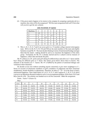
![Inventory Control 397397397397397
q0 = )/2( 13 CC λ × )( 21 CC + / C2 = ]40.2/)90001002[( ×× × )540.2( + / 5 = 000,10,11
= 1,053 units per run.
Total cost including material cost = C0 = 9000 × 1 + )/( 212 CCC + × λ312 CC =
Rs. 9000 + )900010040.22( ××× = Rs. 9,000 + Rs. 1,710 = Rs. 10, 710/- per year.
Number of orders per year = N = λ /q0 = 9,000 / 1,053 = 8.55 orders = App. 9 orders
Time between orders = t0 = 1 / N = 1 / 8.55 = 0.117 year = 64.6 days = App. 65 days.
Problem 8.32.
A manufacturing firm has to supply 3,000 units annually to a customer, who does not have
enough storage capacity. The contract between the supplier and the customer is if the supplier fails to
supply the material in time a penalty of Rs. 40/- per unit per month will be levied. The inventory holding
cost amounts to Rs. 20/- per unit per month. The set up cost is Rs. 400/- per run. Find the expected
number of shortages at the end of each scheduling period.
Solution
Data: C1 = Rs. 20/- per unit per month, C2 = Rs. 40/- per unit per month, C3 = Rs. 400/- per run,
λ = 3000 units per year = 3000 / 12 = 250 units per month = r.
Imax = S = )]/([ 212 CCC + × 13 /2 CrC = ]40/)4020/(40[ + × )2504002( ×× / 20 = 82
units.
q0 = )( 21 CC + / C2 × rC32( / C1) = ]40/)4020[( + × )2504002( ×× / 20 = 123 Units.
Number of shortages per period = q0 – S0 = 123 – 82 = 41 units per period.
Problem 8.33.
The demand of a chemical is constant and at the rate of 1,00,000 Kg per year. The cost of
ordering is Rs. 500/- per order. The cost per Kg of chemical is Rs. 2/-. The shortage cost is Rs.5/- per
Kg per year if the chemical is not available for use. Find the optimal order quantity and the optimal
number of back orders. The inventory carrying cost is 30 % of average inventory.
Solution
Data: λ = 1,00,000 Kg per year, p = Rs. 2/ per Kg., C2 = Rs. 5/- per Kg per year, C3 = Rs. 500
per order, C1 Rs. 2 × 0.30 = Rs. 0.60 per Kg. per year.
q0 = ]/)[( 221 CCC + × )/2( 13 CC λ = ]5/)560.0[( + × )000,00,15002( ×× /0.60=13,663Kg.
Imax = S0 = [C2 / (C1 + C2)] × q0 = [5 / (0.60 + 5)] × 13,663 = 12, 199 Kg.
Optimum back order quantity = q0 – S0 = 13,663 – 12, 199 = 1,464 Kg.
Problem 8.34.
The demand for an item is 18,000 units annually. The holding cost is Rs. 1.20 per unit time and
the cost of shortage is Rs. 5.00. The production cost is Rs. 400/- Assuming that the replenishment rate
is instantaneous determine optimum order quantity.](https://image.slidesharecdn.com/operationsresearch-151024043006-lva1-app6892/85/Operations-research-408-320.jpg)
![398398398398398 Operations Research
Solution
Data: λ = 18, 000 units per year, C1 = Rs. 1.20 per unit, C2 = Rs. 5/- and C3 = Rs. 400/-
q0 = )/2( 13 CC λ × )( 21 CC + / C2 = )000,184002( ×× / 1.20 × )520.1( + / 5 = 3857 units.
t0 = q0 / λ = 3857 / 18,000 = 0. 214 year = App. 78 days.
Number of orders = N = λ / q0 = 18000 / 3857 = 4.67 orders = App. 5 orders.
Problem 8.35.
The demand for an item is deterministic and constant over time and it is equal to 600 units per
year. The per unit cost of the item is Rs. 50/- while the cost of placing an order is Rs. 5/-. The
inventory carrying cost is 20% of the cost of inventory per year and the cost of shortage is Re.1/- per
unit per month. Find the optimal order quantity when stock outs are permitted. If stock outs are not
permitted what would be the loss to the company.
Solution
Data: λ = 600 units, i = 0.20, p = Rs. 50, C1 = ip = 0.20 × 50 = Rs. 10/-, C3 = Rs. 5/-, C2 = Re. 1/-
per month = Rs. 12/ per unit per year.
q0 = )/2 13 CC λ × 221 /)( CCC + = 10/)60052( ×× × 12/)1210( + = 77.46 × 1.35 = 104.6
units.
Maximum number of back orders = q0 × C2/C1 + C2 = S0 = 12 / (10 + 12) × 104.6 = 0.55 × 105.6
= 57.05 units. = App. 57 units.
Expected yearly cost C0 = )2( 13 λCC × C2 / (C1 + C2) = )6005102( ××× × (12 / 10 + 12) =
245 × 0.55 = 134.75 = App. Rs. 135/-
If back orders are not allowed, q0 = 13 /)2( CC λ×× = 10/)60052( ×× = 24. 5 units.
Total cost C0 = )2( 13 λ××× CC = )6001052( ××× = 60000 = Rs. 245/-
Hence the additional cost when backordering is not allowed is Rs. 245 - Rs.135 = Rs. 110/-
Problem 8.36.
The demand for an item is 12,000 units per year and shortages are allowed. If the unit cost is
Rs. 15/- and the holding cost is Rs. 20/- per unit per year. Determine the optimum yearly cost. The cost
of placing one order is Rs. 6000/- and the cost of one shortage is Rs.100/- per year.
Solution
Data: λ = 12,000 units, C1 = Rs. 20/- per unit per year, C2 = Rs. 100/- per year, C3 = Rs. 6000/-
per order. P = Rs. 15/-
q0= 13 /)2( CC λ × 221 /)( CCC + = 20/)000,1260002( ×× × 200/)10020( + = 2939
units.
Number of orders per year = λ / q0 = 12,000 / 2939 = 4.08 = App. 4 orders.
Number of shortages = z0 = q0 × [C1/(C1 + C2)] = 2939 × [20/(20 + 100)] = 489 units.](https://image.slidesharecdn.com/operationsresearch-151024043006-lva1-app6892/85/Operations-research-409-320.jpg)
![Inventory Control 399399399399399
Total yearly cost = p × λ + )2( 13 λCC + )]/([ 212 CCC + =
15 × 12,000 + )000,122060002( ××× × )120/100( = Rs. 1, 08, 989.79 = App. Rs.1, 08, 990
Problem 8.37.
A commodity is to be supplied at the constant rate of 200 units per day. Supplies of any amount
can be had at any required time but each ordering costs Rs. 50/-. Cost of holding the commodity in
inventory is Rs. 2/- per unit per day while the delay in the supply of the item induces a penalty of Rs.10/- per
unit per delay of one day. Find the optimal policy, q and t, where t is the reorder cycle period and q is
the inventory level after reorder. What would be the best policy if the penalty cost becomes infinity?
Solution
Data: C1 = Rs. 2/- per unit per day, C2 = Rs. 10/ per unit per day, C3 = Rs. 50/- per order, r = 200
units per day.
q0 = )/2( 13 CrC × 221 /)( CCC + = 2/)200502( ×× × 2/)102( + = 110 units.
t0 = q0 / r = 110 / 200 = 0.55 day.
The optimal order policy is q0 = 110 units and the ordering time is 0.55 day.
In case the penalty cost becomes ∞ , then q0 and t0 are:
q0 = 13 /2 CrC = 2/)200502( ×× = 100 units.
t0 = q0 / r = 100 / 200 = 0.5 day.
Problem 8. 38.
A Contractor supplies diesel engines to a truck manufacturer at the rate of 20 per day. He has to
pay penalty of Rs. 10/- per engine per day for missing the schedule delivery rate. Holding cost of a
complete engine is Rs. 12/- per month. The manufacturing of engines starts with the beginning of the
month and is completed at the end of the month. What should be the inventory level at the beginning of
each month?
Solution
Data: r = 20 engines per day, C1 = Rs. 12 per month = Rs. 12/30 = Rs. 0.40 per engine per day,
C2 = Rs. 10/- per engine per day, t = 1 month = 30 days.
S0 = Max. Inventory = [(C2)/(C1 + C2)] q0 = [(C2) / (C1 + C2)] × r × Max inventory =
[(10) / (10 + 0.40)] × 20 × 30 = 577 engines per month.
(b) Lost – Sales shortages
In the above case, due to shortages, back orders are allowed, i.e. the demand will be satisfied after the
receipt of the material. But in the present case the assumption is the sales will be lost if there is a
shortage. This is shown in figure 8.14. In this case, the unit shortage cost is proportional to quantity
only and is independent of time as the shortages of any item is the shortage forever not for a finite
interval of time. The shortage cost C2 includes the loss of profit.](https://image.slidesharecdn.com/operationsresearch-151024043006-lva1-app6892/85/Operations-research-410-320.jpg)
![400400400400400 Operations Research
Figure 8. 14.
h = Stick out period. And 0 ≤ h ≤ ∞ hence t = (q/r) + h = (q + rh) / r, where r = uniform rate
of demand.
Carrying cost = (q /2) q × (1/r) C1 = (q2 / 2) × (1/r) C1 = (C1q2) / 2r
Shortage cost = C2 × rh and set up cost = C3
Total cost per cycle = (C1q2) /2r + C2rh + C3
Average total cost per unit of time = [(C1q2) / 2 (q + rh)] + [(C2r2h) / (q + rh)] + [(C3r) / (q + rh)
= C(q,k)
Equating dC(q,k) / dq = 0 and simplifying we get,
q0 = 131
2
22 /)]}2()([({ CrCCrCrC −±
h = rCrCCrCrC 131
2
22 /)]}2()[({ −±−
Problem 8.39.
The demand for an item is continuous and deterministic at 200 units per month. The holding cost
is Rs. 2/- per unit per month and ordering cost is Rs. 5/- per order. In case of shortage, the loss of sales
causes a loss of profit to an extent of Rs. 200/ per month. Find the optimal order quantity.
Solution
Data: r = 200 units, C2 = Rs. 20 / month, C1 = Rs.2/- per unit per month.C3 = Rs. 5 /- per order.
q0 = 131
2
22 /)]}2(([({ CrCCrCrC −± = −×±× 2
)200200([200200{( }2/)]200522( ×××
q0 = )]}2/4000()40000[)40000{( 2
−± = )]}2000)1600000000(40000 −±
= 9.3999940000 ±](https://image.slidesharecdn.com/operationsresearch-151024043006-lva1-app6892/85/Operations-research-411-320.jpg)
![Inventory Control 401401401401401
8.7.10. Economic Order quanity for finite rate of replenishment of inventory with
back orders permitted
As in the previous finite rate of replenishment model, the rate of replenishment is at the rate of ‘k’ units
per unit of time and shortages are allowed. The figure 8.14 shows the graphical representation of the
model.
Figure 8.15.
From the figure, total cost per cycle = C = (S/2) × (t1 + t2) × C1 + (z/2) × (t3 + t4) × C2 + C3
Now, S = t1 (k + r) or t1 = S / (k – r), similarly, t2 = (S / r), t3 = (z / r), and t4 = (z / k – r ),
Substituting the values and simplifying, The cost function becomes,
C = C3 + (C1S2 + C2 z2) / {2 r [1 – (r / k)]}
Hence cost per unit of time (by substituting t = (q / r) = C0 (s,t) = C3 r / q + (C1S2 + C2 z2) / {[2q
( 1 – (r / k)]
After mathematical treatment, the optimal value of C0 (q0,z0) =
C0 (q0,z0) = )}/(1[2{ 13 krrCC − × (C2 / C1 + C2) OR
C0 (q0,x0) = )/( 212 CCC + × krk /)( − × rCC 312
The other models are:
q0 = )/2( 13 CrC × [(C1 + C2) / C2 {1 – (r/k)}] OR
q0 = 221 /)( CCC + × )/( rkk − × 13 /)2( CrC
z0 = )]()}/(1{2[ 212/13 CCCCkrrC +− OR z0 = C1 / (C1 + C2) × (k – r) / k × q0
t0 = (q0 / r) = )(2 213 CCC + /C1C2 r [1 – (r/k)] OR](https://image.slidesharecdn.com/operationsresearch-151024043006-lva1-app6892/85/Operations-research-412-320.jpg)
![402402402402402 Operations Research
t0 = q0 / r = 221 /)( CCC + × )/( rkk − × rCC 13 /2
As we know that S = [q (1 – r/k) – z] we can get,
S0 = )]/(1[2 3 krrC − × [C2 / C1 (C1 + C2)] OR
Max Inv = S0 = )/( 212 CCC + × krk /)( − × 13 /)2( CrC
(Note: By keeping k = ,∞ C2 = ∞ and k = ,∞ the above models reduces to the models without
shortages.).
Problem 8.40.
The demand for an item in a company is 18,000 units per year, and the company can produce the
item at a rate of 3,000 items per month. The cost of one setup is Rs. 500/- and holding cost of one unit
per month is 15 paise. The shortage cost of one unit is Rs. 20/- per year. Determine the optimum
manufacturing quantity and the number of shortages. Also determine the manufacturing time and the
time between setups.
Solution
Data: λ = 18,000 units per year, or r = 1,500 units per month, k = 3000 units per month, C1 = Rs.
0.15 per unit per month, C2 = Rs. 20 /- per unit per year = Rs. 1.67 per unit per month, C3 = Rs. 500/
- per set up.
q0 = 221 /)( CCC + × )/( rkk − × 13 /2 CrC =
67.1/)67.115.0( + × )15003000/(3000 − × 15.0/)15005002( ×× = 4,669 units.
Max inventory = Imax = )/( 212 CCC + × krk /)( − × =13 /2 CrC
)67.115.0/(67.1 + × 3000/)500,13000( − × 15.0/)15005002( ×× = 2,142 units.
Therefore, number of shortages = q0 – Imax = 4669 – 2142 = 2,527 units.
Manufacturing time = q0 / k = 4667 / 3000 = 1.56 months.
Time between setups = t0 = q0 /r = 4669 / 1500 = 3.12 months. = App. 3 months.
Problem 8.41.
The demand for an item in a company is Rs. 12,000 per year and the company can produce the
item at a rate of 2000 units per month. The cost of one setup is Rs. 400/- and the holding cost is 15
paise per unit per month. The shortage cost of one unit is Rs. 20/- per year. Unit cost of material is
Rs. 4/- Determine q0, C0 (q,s), Maximum inventory, Manufacturing time interval, Total time interval.
Solution
Data: λ = 12,000 units per year, k = 2000 units per month or 24000 units per year, C1 = Rs. 0.15
x `12 = Rs. 1.80 per unit per year, C2 = Rs. 20/- per year, C3 = Rs. 400/- per set up. P = Rs. 4/- per unit.
q0 = 13 /)2( CC λ × 221 /)( CCC + × )/( rkk −
= )120004002( ×× × 20/)208.1( + × )1200024000/(24000 − = 3, 410 units.](https://image.slidesharecdn.com/operationsresearch-151024043006-lva1-app6892/85/Operations-research-413-320.jpg)
![Inventory Control 403403403403403
C0 (q,s) = Material cost + inventory cost = 12,000 × 4 + )2( 31 λ××× CC × )/ 212 CCC +
× krk /)( −
= 48,000 + )000,124008.12 ××× + )8.120/(20 + × 12000/)1200024000( −
= Rs. 50,815 per year.
Imax = Maximum inventory = 13 /)2( CC λ × )( 212 CCC + × krk /)( −
= 80.1/)120004002( ×× × )2080.1/(20 + × )000,12000,24( − /24000
= 1564 units/ per setup.
Manufacturing time interval = t1 + t4 = q0 / k = 3410 / 24000 = 0.1421 year = 51.86 days = App.
52 days.
Total time interval = t0 = q0/ λ = 3410/12000 = 0.2842 year = 103.73 days = App. 104 days.
8.7.11. FixedTime Model
In this case, the production is instantaneous and the shortages are allowed and the inventory is to be
replaced at a fixed interval, say at time ‘t’. This appears to be similar with the model, where production
is instantaneous and back orders are allowed (8.7.9.1). The difference between the two models is that
in this model the cycle time for one period is fixed. The graphical representation of the model is given
in figure number 8.16.
As the period is fixed, quantity ‘q’ is known exactly and is equals to ‘rt’. The decision variable is
level of inventory ‘S’ and the level of shortage.
Carrying cost = (S/2) × t1 × C1
Shortage cost = [(q – S) /2] × t2 × C2
Figure 8.16.](https://image.slidesharecdn.com/operationsresearch-151024043006-lva1-app6892/85/Operations-research-414-320.jpg)
![404404404404404 Operations Research
From the triangles, OAB and FBD, the relations are:
(t1/t) = (S/q) or t1 = (S/q) t and t2 = (q – S) t/q
Hence we can write the total cost equation as:
C(S) = (C1 S2) 2r + [C2 (rt - S)2] / 2r by differentiating and equating to zero, we get,
S0 = rt × [(C2) / (C1 + C2)]
Problem 8.42.
A contractor has to supply Diesel engines to a Truck manufacturing company at a rate of 20 per
day. The penalty in the contract is Rs. 10/- per engine per day late for missing the scheduled delivery
date. The cost of holding an engine in stock for one month is Rs. 15/-. His production process is such
that each month (30 days) he starts a batch of engines through the agencies and all are available for
supply after the end of month. What should inventory level be in the beginning of each month?
Solution
Data: C1 = Rs. 15/- / 30 days (Rs. 15/30 per day), C2 = Rs. 10/- per day, r = 20 engines, t = 30
days.
S0 = [rt (C2)] / (C1 + C2) = 20 × 30 × 10 / 10 + (15/30) = 571.4 = App. 571 engines.
8.8. MODELS WITH RESTRICTIONS
8.8.1. Multi- Item, Deterministic Models with one Linear Constraint
Sometimes business may face problems of purchasing many items and storing them when there are
some restrictions regarding the capital to be invested, or storage space etc., Here the materials manager
has to workout the optimal quantity for each material which minimizes the total inventory cost under
given limitations. Due to limitations, may be space or may be capital to be invested, there exists a
relation among items, hence they cannot be considered separately. To simplify the procedure, we use
Lagrange’s multiplier technique as explained below:
Procedure: First neglect the constraint and solve the problem. Then consider the effect of constraint
on solution.
Let number of items is ‘n’. The assumed condition is instantaneous production and no lead-time
and the demand is deterministic and uniform at the rate of ‘ri’ items per unit of time for ‘i th’ item. Let
C1 be the inventory carrying cost per unit of quantity per unit of time for ‘i th’ item and C3 is the set up
cost per run for the ‘i th’ item. As the no shortages are allowed C2 = 0. The cost for ‘i th’ item per unit
of time is:
C0i = (qi / 2) / C1i + (ri / qi) C3i here subscript ‘i’ indicates the costs and quantity of ‘i th’ item
stocked at the beginning of the cycle.
Hence total cost per unit of time: C = C(q1,q2,…..qn) = iiii
n
i
i CqrCq 31
1
)/()2/[( +∑=
),/()2/(/ 2
31 iiiii qrCCqC −=∂∂ where i = 1,2,3,….n.
By equating iqC ∂∂ / to zero, we get, qi0 = iii CrC 13 /)2( × which gives the optima value of q1
where i = 1, 2, 3, …..n.](https://image.slidesharecdn.com/operationsresearch-151024043006-lva1-app6892/85/Operations-research-415-320.jpg)
![Inventory Control 405405405405405
8.8.2. Restriction on the Number of Stocked Units
(Consider a limitation that the average number (of any item is equals to [qi/2] for any
item at any time) of all stocked units should not exceed the number ‘I’, i.e.
∑=
≤
n
i
iq
1
.1)2/1(
Now we have to minimize C, subject to if
∑=
≤
n
i
iq
1
0 |,)2/1( then the optimal value qi0 given above are the required values without any problem.
if, ∑=
≤
n
i
iq
1
0 |,)2/1( is not satisfied, we use the Lagrange’s multiplier technique. The multiplier
function is ∑∑ ==
−λ++=
n
i
i
n
i
iiiii qqrCCqL
11
31 ],2[]/)()2/[( where λ is a Lagrange’s multiplier.
By finding iqL ∂∂ / and λ∂∂ /L and equating them to zero, we get q0 = )]2/()2[( 13 λ+iii CrC
gives the optimal value when they satisfy the condition ∑=
=−
n
i
iq
1
0|2 OR ∑=
=
n
i
iq
1
|2 This constraint
is used to find the value of i by trial and error by
interpolation.
(a) Limitation on Investment
Let us assume that the upper limit of investment to be invested on inventory in Rs. is M. Let pi be the
unit price of ‘i’ th item. Then:
∑=
≤
n
i
ii Mqp
1
Now our problem is to minimize the total cost given in the cost equation in 8.8.1 subject to an
additional cost constraint given above. By analyzing carefully, we can get two cases.
Case1
When ∑=
≤
n
i
ii Mqp
1
0 where qi0 is the optimal quantity given by the equation shown in 8.8.2. This
case does not give any trouble as the optimal order quantity can be found by the equation q0 =
./)2( 13 CrC
Case 2
When ∑=
>
n
i
ii Mqp
1
0 where q0 = .13 /)2( CrC Here suppose qi0 for i = 1,2,3 …n are not the
required optimal values of ‘q’, we have to use Lagrange’s multiplier technique as shown below:](https://image.slidesharecdn.com/operationsresearch-151024043006-lva1-app6892/85/Operations-research-416-320.jpg)
![406406406406406 Operations Research
∑ ∑= =
−λ+×+×=
n
i
n
i
iiiiiii MqpCqrCqL
1 1
31 ],[])/()2/[( where λ is Lagrange‘s multiplier. By
finding λ∂∂ /L and equating it to zero we get,
qi0 = ]2/()2[( 13 iiii pCrC ×λ+
and ∑=
=×
n
i
ii Mqp
1
0 , which says that investment constraint must be satisfied.
Problem 8.43.
A company producing three items has a limited storage space of averagely 750 items of all types.
Determine the optimal production quantities for each item separately, when the following information is
given.
Products
Cost. 1 2 3
Carrying cost C1 Rs. 0.05 0.02 0.04
Setup cost C3 Rs. 50 40 60
Demand = r units. 100 120 75
Solution
Let us first ignore the space constraint imposed and find the optimal order quantities of each item.
Data: Product 1: C1 = 0.05, C3 = Rs. 50, Demand r = 100 units.
Product 2. C1 = 0.02, C3 = Rs. 40/-, r = 120 units.
Product 3 C1 = 0.04, C3 = Rs. 60/-, r = 75 units.
q01 = 11131 /)2( CrC = 05.0/)100502( ×× = 100 × 20 = 447 units.
q02 = 12232 /)2( CrC = 02.0/)120402( ×× = 100 48 = 693 units.
q03 = 13333 /)2( CrC × = 04.0/)75602( ×× = 100 5.21 = 474 units.
Total average inventory at any time = (447/2 + 693 /2 + 474 /2) = 802 units.
This exceeds 750 units the given constraint. We have to find the Lagrange’s Multiplier by trial and
error.
q01 = )]2/)2( 13 λ+CrC = )]005.0205.0/()100502[ ×+×× = 100 67.16 = 409 units.
Where value of λ is taken as 0.005. Similarly,
q02 = )]005.0202.0/()120402[( ×+×× = 100 32 = 566 units.
q03 = )]005.0204.90/)75602[( ×+×× = 100 18 = 424 Units.
Average inventory level = q01 /2 + q02 /2 + q03 /2 = (409 /2 + 566 /2 + 424 / 2) = (204.5 + 283 +
212) = 699.5 = App. 700 units.
This value is less than the give constraint. We can test the above with the value of λ = 0.004,
0.003, 0.002 and 0.001 etc. We can construct a graph for value of λ against the average inventory](https://image.slidesharecdn.com/operationsresearch-151024043006-lva1-app6892/85/Operations-research-417-320.jpg)
![Inventory Control 407407407407407
level. From this graph we will be in a position to find the exact value of λ . When we get an arc in the
graph, we can connect the two ends of the arc and draw straight line, which will help us to find the
value of λ . Figure 8.17 is the graph showing the value of λ on X – axis and the value of average
inventory level on Y - axis.
Figure 8.17. λ Vs Average inventory.
From the figure
(DB/OC) = (DA/OA) or (DB/0.005) = 52 / 100) or λ = DB = (52 / 100) × 0.005 = 0.00256. By
applying this value of λ we get the inventory levels as:
q01 = )00256.0205.0/()100502( ×+×× = 05512.0/10000 = 426 units
q02 = )00256.0202.0/()120402( ×+×× = 02256.0/9600 = 652 units
q03 = )00256.0204.0/()75602( ×+×× = 04256.0/9000 = 460 units
Average inventory level = (426 /2) +(652 / 2) + (460 / 2) = 213 + 326 + 230 = 769
q01 = )]002.0205.0/()100502[( ×+×× = 428 units.
q02 = )]002.0202.0/()120402[( ×+×× = 628 units.
q03 = )]002.0204.0/()75602[( ×+×× = 444 units.
Average level of inventory = (428 / 2) + 628 / 2) + 444 / 2) = 214 + 314 + 222 = 750 units.
Hence optimal inventory of three items is: q01 = 428 units, q02 = 628 units, q03 = 444 units](https://image.slidesharecdn.com/operationsresearch-151024043006-lva1-app6892/85/Operations-research-418-320.jpg)
![408408408408408 Operations Research
Problem 8.44.
For the following data, determine approximately the economic order quantities, when the total
value of average inventory level of the products is Rs. 1000/-
Costs. Product 1. Product 2. Product 3.
Holding Cost C1 (%) 20 20 20
Set up cost C3 in Rs. 50 40 60
Cost per unit = p in Rs. 6 7 5
Yearly demand = r in units. 10000 12000 7500
Solution
Data: C1 = Rs. 20/-, C3 = Rs. 50/-, p = Rs.6/- per unit, r = 10000 units per year for product 1.
C1 = Rs.20/-, C3 = Rs. 40/- p = Rs. 7/- per unit, r = 12,000 units per year for product 2.
C1 = RS.20/-, C3 = Rs. 60/-, p = Rs. 5/- per unit, r = 7500 units per year for product 3.
Investment limit is Rs. 1000/-.
Ignoring constraint, if we find economic order quantity, we have:
q01 = )]20/()10000502[( ×× = 100 5 = App.223 units.
q02 = )]20/()12000402[( ×× = 40 30 = App. 216 units.
q03 = )]20/()7500602[( ×× = 150 2 =App. 210 units.
Value of inventory = (q0i /2) × pi
Corresponding value of average inventory at any time is:
[ (223 / 2) × 6 + (216 / 2) × 7 + 210 / 2) × 5 ] = Rs. 1950/-. This value is greater than the given
financial limit of Rs. 1000/-. Now let us take the value of λ = 5 and find the value of inventory levels.
q01 = )]65220/()10000502[( ××+×× = App. 111 units.
q02 = )]75220/()12000402[( ××+×× = App. 102 units.
q03 = )]55220/()7500602[( ××+×× = App. 113 units.
Corresponding cost of Average inventory level = (111/2) × 6 + 102/2) × 7 + 113/2) × 5 = Rs.
972.50
This amount is slightly less than the given limit. Now let us try the value of λ as 4.
q01 = )]64220/()10000502[( ××+×× = App. 121 units.
q02 = )]74220/()12000402[( ××+×× = App. 112 units.
q03 = )]54220/()7500602[( ××+×× = App. 123 units.
Corresponding cost of Average inventory level = (121/2) × 6 + 112/2) × 7 + 123/2) × 5 = Rs.
1112.50. This is slightly greater than the given limit. Hence the value of λ must lie between 4 and 5. A](https://image.slidesharecdn.com/operationsresearch-151024043006-lva1-app6892/85/Operations-research-419-320.jpg)
![Inventory Control 409409409409409
graph is drawn for values of average inventory cost and λ and a straight line is drawn for the average
inventory cost at λ = 4 and 5 and then a horizontal line from Rs. 1000/- is drawn to find the value of
λ . This is shown in the figure 8.18. From the figure the value of λ is 4.7. Using this value let us find
the value of optimal inventory.
q01 = )]67.4220/()10000502[( ××+×× = App. 114 units.
q02 = )]77.4220/()12000402[( ××+×× = App. 105 units.
q03 = )]57.4220/()7500602[( ××+×× = App. 116 units.
Figure 8.18.
Corresponding cost of Average inventory level = (114/2) × 6 + 105/2) × 7 + 116/2) × 5 = Rs. 999.50.
This amount is very close to the given limit of financial commitment and hence this is accepted.
(Note: In the problems of the type shown above, we are concerned with total value of average
inventories of three products. The constraint in the example is:
½ Σ pi qi ≤ M OR Σ pi qi ≤ 2M. However, the values of qi is worked out by same formula
because by taking this constraint iqL ∂∂ / does not change).
(b) Restrictions on the area available for storage (storage space)
Now let us see when a restriction on storage space in square meters (or square feet) is made how to
solve the problem. Let us assume that ‘a’ is the limit of floor space available in square meters (or](https://image.slidesharecdn.com/operationsresearch-151024043006-lva1-app6892/85/Operations-research-420-320.jpg)
![410410410410410 Operations Research
square feet). Let ai square meters (Square feet) of floor space is required for one of the material, say ‘i
th’ item, then the required constraint is:
∑=
≤
n
i
ii aqa
1
This is formally equivalent to the investment constraint i.e.
n
Σ pi qi ≤ M, for which we have
already obtained optimal order quantity. Hence in place of ‘pi’, if we substitute, ‘ai’ we get:
q0 = )]2/()2[( 13 iiii aCrC λ+
Problem 8.45.
A small shop produces three machine parts 1,2,and 3 in lots. The shop has only 650 square feet
of storage space. The appropriate data for three items are represented fin the following table:
Item Product 1 Product 2 Product 3
Demand rate in units per year 5000 2000 10000
Procurement cost in Rs. 100 200 75
Cost per unit in Rs. 10 15 5
Floor space required in square feet. 0.70 0.80 0.40
The carrying cost on each item is 20% of average inventory valuation per year. If no stock out are
allowed, determine the optimal lot size for each item.
Solution
Q01 = )]/()2[( 131 ipirC = )]102.0/()10050002[( ××× = App. 700 units.
Q02 = )]/()2[( 2232 pirC = )]152.0/()20020002[( ××× = App. 516 units.
Q03 = )]/()2[( 3333 pirC = )]52.0/()75100002[( ××× = App./ 1225 units.
Corresponding floor space required = Σ ai q0i = (0.07 × 707) + 0.8 × 516 + 0.4 × 1225 = 1397.7
square feet. But the given limit is only 650 square feet. Hence the space we got is more than the
required. We can try with Lagrange’s multiples λ to get the right answer. First let us try with the value
of λ = 4.
q0i = )]2/()2[( 3 iiii apirC λ+
q01 = )]70.0421020.0/()10050002[( ××+××× = App. 363 units.
q02 = )]80.0421520.0/()20020002[( ××+××× = App 292 units.
q03 = )]40.042520.0/()75100002[( ××+××× = App 598 units.
Corresponding floor space = (363 × 0.7) + (292 × 0.8) + (598 × 0.4) = 726.9 square feet. As this
area is also more than the given limit, let us try with a value of λ = 5.](https://image.slidesharecdn.com/operationsresearch-151024043006-lva1-app6892/85/Operations-research-421-320.jpg)
![Inventory Control 411411411411411
q01 = )]70.0521020.0/()10050002[( ××+××× = App. 333 units.
q02 = )]80.0521520.0/()20020002[( ××+××× = App 270 units.
q03 = )]40.052520.0/()75100002[( ××+××× = App 578 units.
The required floor space = (333 × 0.7) + (270 × 0.8) + (578 × 0.4) = 668.3 Square feet. This
value is slightly higher than the given limit. Hence by interpolation we can select a slightly higher value
say λ = 5.4. Then the optimal quantities are:
q01 = )]70.04.521020.0/()10050002[( ××+××× = App. 324 units.
q02 = )]80.04.521520.0/()20020002[( ××+××× = App 263 units.
q03 = )]40.04.52520.0/()75100002[( ××+××× = App 531 units.
The required floor space = (324 × 0.7) + (263 × 0.8) + (531 × 0.4) = 649.6 Square feet. This is
very close to the given floor space. Hence the optimal quantities of products are:
q01 = 324 units, q02 = 263 units, and q03 = 531 units.
Problem 8.46.
Three items are produced in a company and they are to be stored in the available space, which is
limited to 25 square meters. The other particulars are given in the table below. Find the optimal quantities
of the products.
Item Demand in units. C3 Procurement cost in Rs, Carrying cost in Rs. Area required in meter square.
1 20 100 30 1
2 40 50 10 1
3 30 150 20 1
Solution
By neglecting the constraint let us find optimal quantities, given by q0i = )]./()2[( 13 iii CrC
q01 = ]30/)201002[( ×× = 11.5 units.
q02 = ]10/)40502[( ×× = 20 units.
q03 = ]20/)301502[( ×× = 21.2 units.
Corresponding space required = 11.5 × 1 + 20 × 1 + 21.2 × 1 = 52.7 Sq.mt. This is more than the
required. Hence let us try the value of λ = 5,15,20 and 30.
λ = 5. for which q0i = iiii aCrC λ+ 2/)2[( 3
q01 = )]15230/()201002[( ××+×× = 10 units.
q02 = )]15210/()40502[( ××+×× = 14.1 units.](https://image.slidesharecdn.com/operationsresearch-151024043006-lva1-app6892/85/Operations-research-422-320.jpg)
![412412412412412 Operations Research
q03 = )]15220/()301502[( ××+×× = 17.3 units.
Corresponding floor area = 10 × 1 + 14.1 × 1 + 17.3 × 1= 41.4 Sq. Mt. This is also more than the
given limit.
Let take the value of λ = 15
q01 = )]115230/()201002[( ××+×× = 8.2 units.
q02 = )]115210/()40502[( ××+×× = 10.2 units.
q03 = )]115220/()301502[( ××+×× = 13.4 units.
Corresponding floor area = 8.2 × 1 + 10.2 × 1 + 13.4 × 1= 31.8 Sq. Mt. This is also more than the
given limit.
Now let try with the value of λ = 20.
q01 = )]120230/()201002[( ××+×× = 7.6 units.
q02 = )]120210/()40502[( ××+×× = 8.9 units.
q03 = )]120220/()301502[( ××+×× = 12.2 units.
Corresponding floor area = 7.6 × 1 + 8.9 × 1 + 12.2 × 1= 28.7 Sq. Mt. This is also more than the
given limit.
Now let take the value of λ = 30.
q01 = )]130230/()201002[( ××+×× = 6.7 units.
q02 = )]130210/()40502[( ××+×× = 7.6 units.
q03 = )]130220/()301502[( ××+×× = 10.6 units.
Corresponding floor area = 6.7 × 1 + 7.6 × 1 + 10.6 × 1= 24.9 Sq. Mt. This is very close to the
given limit. Hence the optimal quantities of three items are: q0l = 6.7 units, q02 = 7.6 units and q03 = 10.6
units.
Problem 8.47.
A machine shop produces three products 1,2 and 3 in lots. The shop has a warehouse whose
total floor area is 4000 square meters. The relevant data for three products is given below:
Item Product 1 Product 2 Product 3.
Annual demand in units per year (r) 500 400 600
Cost per unit (p) in Rs. 30 20 70
Set up cost per lot C3 in Rs. 800 600 1000
Floor area required in Sq. mt. 5 4 10
The inventory carrying chargers for the shop are 20% of the average inventory valuation per
annum for each item. If no stock outs are allowed and at no time can the warehouse capacity be
exceeded, determine the optimal lot size of each item.](https://image.slidesharecdn.com/operationsresearch-151024043006-lva1-app6892/85/Operations-research-423-320.jpg)
![Inventory Control 413413413413413
Solution
Optimal quantities of each item is given by (ignoring the limitation on floor area): )]./()2[( 3 iprC ii ×
q01 = )]3020.0/()5008002[( ××× = App. 365 units.
q02 = )]2020.0/()4006002[( ××× = App 346 units.
q03 = )]7020.0/()60010002[( ××× = App. 292 units.
Floor space required = Σ q0i ai = 365 × 5 + 346 × 4 + 292 × 10 = 1825 + 1384 + 2920 = 6129
Sq. mt. This is greater than the given limit of 4000 Sq.mt. Let us use Lagrange’s multiplier technique to
find the required quantities. Let us try with values of λ = 1.0, 0.8.
λ = 1.00, q0i = )]2/()2[( 3 iiii apirC ×λ×××××
q01 = )]5123020.0/()5008002[( ××+××× = 223 units.
q02 = )]4122020.0/()4006002[( ××+××× = 200 units.
q03 = )]10127020.0/()60010002[( ××+××× = 187 units.
Required floor area = 223 × 5 + 200 × 4 + 187 × 10 = 3785 Sq. mt. This is also less than the given
limit.
λ = 0.8, q0i = )]12/()2[( 3 iiii pirC ×λ×××××
q01 = )]58.023020.0/()5008002[( ××+××× = 239 units.
q02 = )]48.022020.0/()4006002[( ××+××× = 214 units.
q03 = )]108.027020.0/()60010002[( ××+××× = 200 units.
Required floor area = 239 × 5 + 215 × 4 + 200 × 10 = 4051 Sq.mt. This is slightly higher than the
given limit. Now let us take the value of λ = 0.835 and find the optimal values of quantities.
q01 = )]5835.023020.0/()5008002[( ××+××× = 236 units.
q02 = )]4835.022020.0/()4006002[( ××+××× = 211 units.
q03 = )]10835.027020.0/()60010002[( ××+××× = 197 units.
Required floor area = 236 × 5 + 211 × 4 + 197 × 10 = 3994 Sq mt. This is very nearer to given
value, hence is accepted. Hence q01 = 236 units, q02 = 211 units and q03 = 197 units. (Remember
always see that the obtained area must be slightly less than or equal to the given limit and it
should never exceed the given value.)
8.9. PROBABILISTIC OR STOCHASTIC MODELS
So far we have discussed the problems, where the demand for an item is known and deterministic in
nature and it will not vary during the planning period. If the demand is not known exactly to us or it](https://image.slidesharecdn.com/operationsresearch-151024043006-lva1-app6892/85/Operations-research-424-320.jpg)
![414414414414414 Operations Research
cannot be pre determined or in case it goes on changing / fluctuate with time in either way, the situation
is known as Models with unknown demand or models with probabilistic demand. This means that
demand can be known with certain probability. When the probability of demand ‘r’ is expected, then
we cannot minimize the actual cost. But the optimal quantity of inventory is determined on the basis of
minimizing the total expected cost represented by (TEC) instead of minimizing the actual cost. In
many practical situations or in real world problems, it is observed that neither the consumption rate of
material or commodity or the lead time is constant throughout the year. To face these uncertainties in
consumption rate and lead time, an extra stock is maintained to meet the demand, in case any shortage
is there. The extra stock is termed as BUFFER STOCK OR SAFETY STOCK.
8.9.1. Single period model with uniform demand (No set up cost model)
In this model the following assumptions are made:
(a) Reorder time is fixed and known say ‘t’ units of time. Therefore the set up cost C3 is not
included in the total cost.
(b) Demand is uniformly distributed over period. Here the term period refers for the time of one
cycle.
(c) Production is instantaneous, i.e. lead-time is zero.
(d) Shortages are allowed and they are backlogged. The costs included in this model is C1
carrying cost per unit of quantity per unit of time and C2 the shortage cost per unit of
quantity per unit of time.
(e) Units are discrete and p(r) is the probability of requiring ‘r’ units per period.
If ‘S’ is the level of inventory in the beginning of each period, and we have to find the optimum
value of ‘S’. Hence the decision variable is S.
In this problem two situations will arise:
(a) Demand r ≤ S, (b) demand r > S. The two situations are illustrated by means of graph in
figure 8.19.
Inventory in one cycle = ½ (S + S – r) t = ½ (2S – r) t = (S – r/2) t. units.
Hence inventory Carrying cost = C1 × (S – r/2) × t, this is true when r ≤ S. But the demand is
equal to ‘r’ is with a probability of p (r). Hence the expected carrying cost = C1 × (S – r/2) × t × p (r).
As ‘r’ may have any values (because r ≤ S), the total expected carrying cost when r ≤ S is given by:
∑=
×−×
S
r
rprSctC
0
1 )()2/(
In case r > S, then carrying cost and shortage cost are to be considered.
Carrying cost = ½ × S × t × C1 and shortage cost = ½ (r – S) × C2 t2
By mathematical treatment (Students are advised to refer for derivation the Operations Research
book where mathematical approach is given), it can be shown that
L (S0 – 1) < [(C2) / (C1 + C2)] < L (S0), where, L (S) = ∑ ∑=
∝
+=
×++
S
r Sr
rrpSrp
0 1
]/)([½)()(](https://image.slidesharecdn.com/operationsresearch-151024043006-lva1-app6892/85/Operations-research-425-320.jpg)
![Inventory Control 415415415415415
Total expected cost is given by the formula:
C(s) = ∑ ∑∑
∞
+=
∞
+==
×−+××+−
1 1
2
2
2
1
0
1 )(]2/)[()()2/()()]2/([
Sr Sr
S
r
rprSrCrprSCrPrSC
Figure 8.19](https://image.slidesharecdn.com/operationsresearch-151024043006-lva1-app6892/85/Operations-research-426-320.jpg)
![416416416416416 Operations Research
Problem 8.48.
A contractor of second hand motor trucks uses to maintain a stock of trucks every month. The
demand of the trucks occurs at a constant rate but not in constant size. The probability distribution of
the demand is as shown below:
Demand (r): 0 1 2 3 4 5 6 or more.
Probability p (r): 0.40 0.24 0.20 0.10 0.05 0.01 0.00
The holding cost of an old truck in stock for one month is /Rs.100/- and penalty for a truck if not
delivered to the demand, is Rs. 1000/-. Determine the optimal size of the stock for the contractor.
Solution
S R P (r) [p (r)/r] ∑
∞
+1
/)([
S
rrp (S+1/2) × ∑
∞
+1
]/)([
S
rrp ∑
S
rp
0
)( L (S)
0 0 0.40 ∞ 0.3875 0.19375 0.40 0.59375
1 1 0.24 0.2400 0.1475 0.22125 0.64 0.86125
2 2 0.20 0.1000 0.0475 0.11875 0.84 0.95874
3 3 0.10 0.0330 0.0145 0.05075 0.94 0.99075
4 4 0.05 0.0125 0.0020 0.00900 0.99 0.99900
5 5 0.01 0.0020 0.0000 0.00000 1.00 1.00000
≥6 ≥6 0.00 0.0000 0.0000 0.00000 1.00 1.00000
Here the ratio [C2 / (C1 + C2)] = [1000 / (1000 + 100) = 1000 / 1100 = 0.9090. This figure lies
between L (2) and L (1). Hence the optimal stock = 2 trucks.
Problem 8.49.
A manufacturer wants to determine the optimum stock level of a certain part. The part is used in
filling orders, which come in at a constant rate. The delivery of these parts to him is almost instantaneous.
He places his orders for these parts at the start of every month. The requirements per month are
associated with probabilities shown in table below. Holding cost is Re.1/- per part per month and
shortage cost is Rs. 19/- per part per month. Also find the expected cost associated with the optimum
stock.
Demand in number
of parts required per month: 0 1 2 3 4 5 6 or more.
Probability: 0.10 0.15 0.25 0.30 0.15 0.05](https://image.slidesharecdn.com/operationsresearch-151024043006-lva1-app6892/85/Operations-research-427-320.jpg)
![Inventory Control 417417417417417
Solution
S R P (r) [p (r)/r] ∑
∞
+1
/)([
S
rrp (S+1/2) × ∑
∞
+1
]/)([
S
rrp ∑
S
rp
0
)( L (S)
0 0 0.10 ∞ 0.4225 0.21125 0.10 0.31125
1 1 0.15 0.1500 0.2725 0.40875 0.25 0.65875
2 2 0.25 0.1250 0.1475 0.36875 0.50 0.86875
3 3 0.30 0.1000 0.0475 0.16625 0.80 0.96625
4 4 0.15 0.0375 0.0100 0.04500 0.95 0.99500
5 5 0.05 0.0100 0.0000 0.00000 1.00 1.00000
6 or > 6 6 or > 6 0.00 0.0000 0.0000 0.00000 1.00 1.00000
Here the ratio C2 / (C1 + C2) = 19 / (19 + 1) = 19 / 20 = 0.95. This lies between (L2) and (L3).
Hence we can take S = 3 units.
The optimal cost is given by:
C(s) = ∑ ∑∑
∞
+=
∞
+==
×−+××+−
1 1
2
2
2
1
0
1 )(]2/)[()()2/()()]2/([
Sr Sr
S
r
rprSrCrprSCrPrSC
= Rs.[ Σ (3 – r/2) × p (r ) + 1 × Σ [(32 / 2 ) × p (r) / r] + 19 3 [ (r–3 )2 / 2r p (r)]
= { [(3 – 0 ) ( 0.10) + ( 3 – ½ ) ( 0.15)] + [(3 – 1) ( 0.25) + (3 – 3/2) ( 0.30)] + (9/2) [ (0.15/ 4)
+ (0.05/4) + 0]
+ 19 [ (4 – 3)2 / (2 × 4) × ( 0.15) + (5 – 3)2 / (2 × 4) × (0.15) + 0]}
= Rs. [ ( 0.30 + 0.375 + 0.50 + 0.45) + 0.21375 + 0.73625] = Rs. 2.58.
Problem 8.50.
The demand for a particular product is continuous and shows the following probability distribution:
Demand: 0 1 2 3 4 5 or more
Probability: 0.16 0.10 0.30 0.24 0.20 0.00
Find out the optimum stock level if the cost of shortage is Rs. 40/- per unit and the cost of
holding is Rs. 10/- per unit. The shortage cost is proportional to both time and quantity short.](https://image.slidesharecdn.com/operationsresearch-151024043006-lva1-app6892/85/Operations-research-428-320.jpg)
![418418418418418 Operations Research
Solution
S R P (r) [p (r)/r] ∑
∞
+1
/)([
S
rrp (S+1/2) × ∑
∞
+1
]/)([
S
rrp ∑
S
rp
0
)( L(S)
0 0 0.16 ∞ 0.38 0.190 0.16 0.350
1 1 0.10 0.10 0.28 0.420 0.26 0.680
2 2 0.30 0.15 0.13 0.325 0.56 0.885
3 3 0.24 0.08 0.05 0.175 0.80 0.975
4 4 0.20 0.05 0.00 0.000 1.00 1.000
5≥ 5≥ 0.00 0.00 0.00 0.000 1.00 1.000
Now the ratio C2 / (C1 + C2) = 40 / (40 + 10) = 0.8.
0.685 < 0.8 < 0.885, in this case S = 2 satisfies the condition. Hence optimum stock level = 2
units.
Problem 8.51.
The probability distribution of monthly sales of a certain item is as follows:
Monthly sale in units: 0 1 2 3 4 5 6
Probability: 0.02 0.05 0.30 0.27 0.20 0.10 0.06
The cost of carrying inventory is Rs. 10/- per unit per month. The current policy is to maintain a
stock of four items at the beginning of each month. Assuming that the cost of shortage is proportional
to both time and quantity short, obtain the imputed cost of a shortage of one item for one unit of time.
Solution
As the data given is in discrete values, the imputed value will have a range.
Data: C1 = Rs. 10/- per unit per month. S = Stock level = 4 units.
As the demand is uniformly distributed over the month,
L (S0 – 1) < C2 / (C1 + C2) < L(S0)
L (S0 – 1) = L (4 – 1) = ∑ ∑= =
×++
4
0
6
4
/)(½)4()(
r r
rrprp
= 0.84 + (7/2) [ (0.20/4) + (0.10 / 5) +(0.06/ 6)] = 0.92
Thus the least value of C2 is given by C2 / (C1 + C2) = 0.92 or (C2 /10) + C2 = 0.92. Which gives
that the value of C2 = Rs. 115/-.
Similarly, the highest value of C2 is given by considering the right-hand side of C2 / (C2 + C2), i.e.
C2 / (C1 + C2) = ∑ ∑= =
×++
4
0
6
5
/)(½)4()(
r r
rrprp = 0.84 + (9 / 2) [ (0.10 / 5) + (0.06 / 6) ] = 0.975.
Hence C2 = 0.975 (10 + C2), because C1 = Rs. 10/-. This gives C2 = Rs. 390/-.
Therefore imputed cost of Shortage is given by Rs. 115/- < C2 < Rs. 390/-](https://image.slidesharecdn.com/operationsresearch-151024043006-lva1-app6892/85/Operations-research-429-320.jpg)
![Inventory Control 419419419419419
Problem 8.52.
The probability distribution of monthly sales of certain item is as follows:
Monthly sales: 0 1 2 3 4 5 6 7 8
Probability: 0.01 0.04 0.25 0.30 0.23 0.08 0.05 0.03 0.01
The cost of holding inventory is Rs.8/- per unit per month. A stock of 5 items is maintained at the
start of each month. If the shortage cost is proportional to both time and quantity short, find the
imputed cost of shortage of unit item for unit time.
Solution
As the given data has discrete units the imputed cost will have a range.
Given that S = 5, C1 = Rs.8/- per unit per month, Range of monthly sales = 0 to 8 and the
probability of sales are as given below:
p0 p1 p2 p3 p4 p5 p6 p7 p8
0.01 0.04 0.25 0.30 0.23 0.08 0.05 0.03 0.01
The range of S is given by: L (S0 – 1) < C2 / (C1 + C2) < L(S0) i.e. The least value of C2 is given
by:
L (S0 – 1) = L (S0 – 1) = ∑∑ ==
×++
8
5
0
4
0
/)(½)()(
rr
rrpSrp
L (5 – 1) = L (5 – 1) = )8/(/)(½)5()( 22
8
5
4
0
CCrrprp
rr
+=×++ ∑∑ ==
(p0 + p1 + p2 + p3 + p4) × (9/2) [ (p5 / 5) + (p6/6) + (p7 / 7) + (p8 / 8 ) ] = C2 / (C1 + C2)
= (0.01 + 0.04 + 0.25 + 0.30 + 0.23) + (9/2) [(0.08/5) + 0.05 / 6) + (0.03 / 7) + (0.01 / 8)
= C2 / (8 + C2)
= 0.83 + 4.5 (0.016 + 0.0083 + 0.0043 + 0.00125) = 0.9643 = C2 /(8 + C2),
C2 = (.9643 × 8) / 0.0357 = Rs. 216/-
Similarly upper limit of C2 can be obtained by C2/(C1 + C2) < L(S0) = C2 / (C1 + C2) =
∑∑ ==
×++
8
6
5
0
/)(½)5()(
rr
rrprp
(p0 + p1 + p2 + p3 + p4 + p5) + (11 / 2) × [ (p6 / 6) + (p7 / 7) + (p8 / 8)] = C2 / ( 8 + C2)
(0.01 + 0.04 + 0.25 + 0.30 + 0.23 + 0.08) + (11 / 2) [ (0.05 / 6) + (0.03 / 7) + (0.01 / 8)]
= C2/(8 + C2)
0.91 + (11/ 2) × (0.01385) = 0.91 + 0.076165 = C2 / (8 + C2)
(8 + C2) × (0.91 + 0.076165) = C2, Which gives C2 = Rs. 570.25
Hence the range of C2, i.e. imputed value = Rs. 216 < C2 < Rs. 570.25](https://image.slidesharecdn.com/operationsresearch-151024043006-lva1-app6892/85/Operations-research-430-320.jpg)
![420420420420420 Operations Research
8.9.2. Single period problem with instantaneous demand (or discontinuous
demand and time independent costs - no set up cost model)
This Model is very much similar to the previous one but here the withdrawal of items form the inventory
is not uniformly distributed over the period and the cost C1 and C2 are independent of time. There are
two cases here.
Case (a)- Demand ‘r’ is ≤ S: Here the cost is (S – r) C1.
Case (b)- Here the demand ‘r’ is > S: In this case we will not consider the holding cost of an item
if it is used or interpret that the demand is fulfilled in the beginning of the period. The cost is (r – S) C2.
Both the cases are illustrated by means of graphs in the figure 8.20.
Here the total expected cost [TEC(s)] = ∑ ∑=
∞
+=
−=−
S
r Sr
rpSrCrprS
0 1
2 )()()()(
The value of optimal value of S = S0 is given when,
TEC (S0 + 1) > TEC (S0) and TEC (S0 – 1) > TEC (S0)
Now TEC (S+1) = ∑ ∑
+
=
∞
+=
−−+−+
1
0 2
21 )()1()()1(
S
r Sr
rpSrCrprSC
Figure 8.20
Similarly, TEC (S – 1) – TEC (S) = ∑
−
=
+−
1
0
212 ).()(
S
r
rpCCC
By mathematical treatment (students are advised to refer to a book on O.R. with mathematical
approach for derivation) we can show that S0 is optimum when,](https://image.slidesharecdn.com/operationsresearch-151024043006-lva1-app6892/85/Operations-research-431-320.jpg)


![Inventory Control 427427427427427
8.11. INVENTORY PROBLEMS WITH UNCERTAIN DEMAND ( MODELS WITH
BUFFER STOCK)
Many a time inventory manager comes across a situation where demand cannot be completely pre-
determined. The demand fluctuates in either way. In fact in many practical situations, we see that both
demand for an item or lead-time, i.e., the time between placing order and procurement of material will
remain constant. In many situations, both demand and lead-time are fluctuating due to uncontrollable
reasons. They are highly uncertain in nature. To face these uncertainties in consumption rate and lead
time, an extra stock is maintained to meet out the demands, if any. This extra stock is generally known
as Safety stock’ or ‘Buffer stock’.
8.11.1. To Determine the Buffer Stock and Re-order Level (ROL)
We must know the maximum lead-time and normal lead-time and the demand during these periods to
estimate the buffer stock or safety stock required. The buffer stock is calculated by multiplying the
consumption rate during the lead – time by the difference between maximum lead-time and normal
lead-time. Let
B = Buffer stock,
L = Lead time,
Ld = Difference between maximum lead-time and minimum lead- time.
r = Demand rate.
Total inventory consumption during lead-time, if buffer stock is not maintained = L × r = Lr.
Thus as soon as stock level reaches ‘Lr’, quantity ‘q’ should be ordered. This point where we
order is known as reorder level or ROL. However due to uncertainty in supply, this policy of ordering
when stock level reaches ‘Lr’ will create shortages and leads to back orders or lost sales. In order to
avoid the shortages, a buffer stock is maintained. Hence,
ROL = Lr + Buffer stock = Lr + B. = Lr + Ld r = (L + Ld) × r
Now maximum inventory = q + B,
Minimum inventory = S
Average inventory = [(q + B) + B] / 2 = (q / 2) + B.
To illustrate the above, let us consider a simple example.
Suppose the demand for an item is 200 units per month, the normal lead-time is 15 days and
maximum lead time is 2 months, then the buffer stock B = (2 - ½ ) × 200 = 300 units.
If L is the lead -time and ‘r’ is the demand, then the inventory during the lead-time = Lr, which is
nothing but the ROL as discussed above. If we maintain buffer stock, then placed an order when stock
level reaches the level = B + Lr. Say for example, the monthly consumption rate for an item is 100 units,
the normal lead time is 5 days and the buffer stock is 150 units, then ROL = 150 + (1/2 + 100) = 200
units.
Optimum Buffer stock: When buffer stock maintained is very low, the inventory holding cost
would be low but the shortages will occur very frequently and the cost of shortages would be very
high. As against this if the buffer stock maintained is rather large, storages would be rather rare,
resulting into low shortage costs but inventory holding costs would be high. Hence it becomes necessary
to strike balance between the cost of shortages and cost of inventory holding to arrive at an Optimum
Buffer Stock.](https://image.slidesharecdn.com/operationsresearch-151024043006-lva1-app6892/85/Operations-research-438-320.jpg)
![428428428428428 Operations Research
Figure 8.21
Problem 8.61.
The average monthly consumption for an item is 300 units and the normal lead-time is one month.
If the maximum consumption has been up to 370 units per month and maximum lead-time is 1 ½
months, what should be the buffer stock for the item.
Solution
Maximum lead – time demand = Maximum lead-time × maximum demand rate = (3/2) × 370 =
555 units.
Normal lead-time demand = 1 × 300 = 300 units.
Buffer stock = Maximum lead-time demand – Normal lead- time demand = 555 – 300 = 255 units.
Problem 8.62.
For a fixed order quantity system find the various parameters for an item with the following data:
Annual demand = λ = 10000 units, Unit price = p = Rs. 1.00, i = Carrying cost = Rs. 0.24 per unit,
C3 = Set up cost = Rs. 12/- per production run, Past lead times in days are = 15,25,13,14,30, 17
days.
Solution
(a) E.O.Q = q0 = ipC /)2( 3λ = 124.0/)12100002( ××× = 1000 units.
(b) Optimum buffer = (Maximum lead- time – Normal lead time) × monthly consumption =
= [(30 – 125) / 30] × 10000 / 12 = 416.66 = App 417 units. (Here the optimum lead-time =
15 days = 15/30 months).](https://image.slidesharecdn.com/operationsresearch-151024043006-lva1-app6892/85/Operations-research-439-320.jpg)
![Inventory Control 429429429429429
Note: for more safety some times it is advisable to round off the buffer stock to 450 units.
Another way of getting the same is:
(Normal lead-time consumption = Norma lead time × monthly consumption = (15/30) ×
(10000/12) = 416.66 or approximately = 417 units).
Hence Re-order level or ROL = Safety stock + normal lead-time consumption = 450 + 417 = 867
or App. 870 units.
The inventory would fluctuate from a maximum, of 1450 to a minimum of 450 units. Hence the
average inventory = (1450 + 450)/2 = 950 units.
Problem 8.63.
A company uses annually 50,000 units of an item each costing Rs. 1.20. Each order costs Rs. 45/
- and inventory carrying costs are 15% of the annual average inventory value. Find EOQ.
If the company operates 250 days a year, the procurement time is 10 days and safety stock is 500
units, find re -order level, maximum, minimum and average inventory.
Solution
Data = λ = 50,000 units, p = Rs. 1.20, i = 15%, C3 = Rs. 45/- L = 10 days, B = 500 units.
q0 = ipC /)2( 3λ = )]20.115.0/()50000452[( ××× = 5000 units.
The company operates 50 days a year. Hence requirement per day = 50000 / 250 = 200 units per
day.
Lead-time demand = 10 × 200 = 2000 units.
Safety stock = 500 units.
Hence ROL = 2000 + 500 = 2500 units.
Maximum inventory = 5000 + 500 = 5500 units.
Minimum inventory = 5000 units.
Average inventory = (5000 / 2) + 500 = 3000 units.
Problem 8.64.
A firm uses every year 12000 units of a raw material costing Rs. 1.25 per units. Ordering cost is
Rs. 15/- per order and the holding cost is 5 % per year of average inventory. (i) Find Economic Order
Quantity,
(ii) The firm follows EOQ purchasing policy. It operates for 300 days per year. Procurement
time is 14 days and safety stock is 400 units. Find the re-order point, the maximum inventory and the
average inventory.
Solution
Data: λ = 12,000 units, p = Rs. 1.25 per units, C3 Rs. 15/-, i = 0.05, Number of working days
= 300, L = 14 days, B = 400 units.
E. O. Q = ipC /)2( 3λ = )]25.105.0/()000,12152[( ××× = 2,400 units.
Re order level = Buffer stock + Consumption during the lead-time = 400 + (12,000 / 300) × 14 =
960 units.](https://image.slidesharecdn.com/operationsresearch-151024043006-lva1-app6892/85/Operations-research-440-320.jpg)
![430430430430430 Operations Research
Maximum inventory = q0 + B = 2400 + 400 = 2800 units.
Minimum inventory = B = 400 units.
Average inventory = (q0 / 2) / B = (2800 / 2) + 400 = 1600 units.
Problem 8.65
Calculate the various parameters when the following data is available for an item, which is maintained
on EOQ system.
Annual consumption = λ = 12000 units, Unit price = Rs. 7.50, Set up cost = Rs. 6.00 per run,
Inventory carrying cost = Rs. 0.12 per unit, Normal lead-time = Ln = 15 days and maximum lead-time
= Lm = 20 days.
Solution
E.O.Q = 13 /)2( CC λ = ]12.0/)1200050.72[( ×× = 1096 units.
Optimum buffer stock = B = (Lm – Ln) × consumption = [(20 – 15) / 30] / (12000 / 12)] = 167
units.
Re-order level = ROL = B + Normal lead-time consumption = 167 + [(15 / 30 × 12) × 12000] =
167 + 500 = 667 units.
Problem 8.66
In an inventory model, suppose that the shortages are not allowed and the production rate is
infinite and the following data is available:
Yearly demand λ = 600 units, Carrying chargers = i = 0.20, C3 = Rs. 80/- per order, p = Rs. 3.00
per unit, Lead-time = L = 1 year.
Solution
q0 = ipC /)2( 3λ = )]320.0/()600802[( ××× = 400 units.
The time of the cycle = t0 = (q0 / λ ) = 400 / 600 = (2/3) year
ROL = B + Normal lead time consumption
Buffer stock = (Maximum lead time – Normal lead-time ) × consumption = ( 1 – 2/3 ) × 600
= ( 1/3) × 600 = 200 units.
Hence ROL = 200 + 1 × 600 = 800 units.
The minimum average yearly cost of ordering and holding = ipC ×λ×× 32(
= )320.0600802( ×××× = Rs. 240/-.
Problem 8.67.
The following is the distribution of lead-time and daily demand during lead-time:
Lead- time in days: 0 1 2 3 4 5 6 7 8 9 10
Frequency: 0 0 1 2 3 4 4 3 2 2 1
Demand per day
in units: 0 1 2 3 4 5 6 7
Frequency: 3 5 4 5 2 3 2 1
What is the buffer stock?](https://image.slidesharecdn.com/operationsresearch-151024043006-lva1-app6892/85/Operations-research-441-320.jpg)

![432432432432432 Operations Research
As t0 is greater than the lead-time, and the safety stocks 400 units, the re-order level will be =
Safety stock + Normal lead-time consumption = 400 + 12 × 80 = 1360 units.
Average inventory = B + (q0 / 2) = 400 + 4000 / 2 = 2400 units.
Maximum inventory = B + q0 = 400 + 4000 = 4400 units.
Minimum Inventory = B = 400 units.
Problem 8.69.
Consider the inventory system with the following data in usual notations: λ = 1000 units pr year,
i = 0.30, p = Rs. 0.50 per unit, C3 = Rs. 10 per order, L = 2 years, Determine (a) E.O.Q, (b) Re order
point, (c) Minimum average cost.
Solution
q0 = ipC /)2( 3λ = )]50.030.0/()1000102[( ××× = 365 units., t0 = q0 / λ = 365/1000 = 0.365
years. = 0.365 × 12 = 4.38 months.
Lead-time is given as 2 years. But optimal time = 4.38 months. Hence re-ordering occurs when
the level of inventory is sufficient to satisfy the demand for (L – t0) = 2 – 0.365 = 1.635 years. Thus
optimum quantity q0 = 365 units is ordered when the re -order of inventory reaches 1.635 × 1000 =
1635 units.
Hence R.O.P = 1635 units.
Minimum average cost = λipC32 = )100050.03.0102( ×××× = Rs. 54.77.
8.12. INVENTORY MODELS WITH VARIABLE PURCHASE PRICE OR PURCHASE
INVENTORY MODELS WITH PRICE BREAKS
Previously in article 8.7.6 we have discussed quantity discount models, where, the seller will offer a
discount on the quantity purchased between certain quantities. The extension of this model is the price
break models. In price break model the seller will offer discounts for the material purchased in a
stepwise manner. This means to say that at every stage i.e., quantity levels, he offers different prices.
For example, let us say the price of material when the quantity purchased is from 1 to 100 Rs. 10 per
unit, from 101 to 300 the price is Rs. 9/- per unit and for quantity above 301 the price will be Rs. 9/-
per unit. This type of purchasing is known as price break models. Mathematically the model is represented
as under:
Quantity purchased ‘q’ Unit purchasing price in Rs.
b0 ≤ q < b1 p1
b1 ≤ q < b2 p2
……………. ………………
……………. …………......
bi –1 ≤ q < bi pi
bn –1 ≤ q < bn pn
(Note: Physically b0 is meaningless as if b = q = 0, then there is no problem of inventory. Hence
we consider lower bound as b0 = 1.)](https://image.slidesharecdn.com/operationsresearch-151024043006-lva1-app6892/85/Operations-research-443-320.jpg)

![434434434434434 Operations Research
Figure 8.22
Problem 8.70 (Single price break)
Find the optimal order quantity for which the price breaks are as follows:
Quantity Unit price in Rs.
0 ≤ q < 500 Rs. 10.00
500 ≤ q < ∞ Rs. 9.25
The monthly demand for the product is 200 units, the cost of storage is 2% of unit cost and the
ordering cost is Rs. 350 per order.
Solution
Data: b0 = 0, λ = 200, I = 0.02, C3 = Rs. 350/- p1 = Rs. 10/-, p2 = Rs. 9.25
q1
0 = 13 /)2( ipC λ = 1002.0/)2003502( ××× = 20.0/140000( = 700000 = 836.6 = 837
units.
This does not fall in the range 0 to 500. Hence we have to take second range.
q2
0 = )]25.902.0/()2003502[( ××× = 870 units. This is in the range 500 to .∞ Let us calculate
the total cost for this quantity.
C2
q = 9.25 × 200 + 350 × (200 / 870) + 0.02 × 9.25 × (870 / 2) = Rs. 1850 + Rs. 80.45 +
Rs.804.75 = Rs. 2735.20](https://image.slidesharecdn.com/operationsresearch-151024043006-lva1-app6892/85/Operations-research-445-320.jpg)
![Inventory Control 435435435435435
Problem 8.71
Find the optimal order quantity for a product for which the price breaks are as follows:
Quantity Price in Rs. per unit.
0 ≤ q < 100 20
100 ≤ q < 200 18
200 ≤ ∞ 16
The monthly demand for the product is 400 units. The storage cost is 20% of the unit cost and
the ordering cost is Rs. 25 per order.
Solution
I = 0.20, C3 = Rs. 25/-, λ = 400,
q3
0 = )]2020.0/)400252[( ××× = 82.5 units = 83 units.
q2
0 = )]1820.0/)400252[( ××× = 74.3 units = 74 units.
q1
0 = )]1620.0/)400252[( ××× = 70 units.
From the above q1
0 = 75 falls in the given range 0 to 100. Hence we have to find the total cost for
75 units at the rate of Rs. 20 per unit and cost of 100 units at the rate of 18 units. Which ever is less that
is taken as the optimal order quantity.
C75
0 = 20 × 400 + 25 × (400 / 70) + 0.20 × 20 × (70 / 2) = Rs. 8282.80
C100
0 = 18 × 400 + 25 × (400 / 100) + 0.20 × 18 × (100 / 2) = Rs. 7480. Let us also find the cost
200 units at Rs. 16/- per unit.
C200
0 = 16 × 400 + (400 / 200) × 25 + 0.02 × 16 × (200 / 2) = Rs. 6770/-
As C200
0 is the minimum, the optimal order quantity is 200 units.
Problem 8.72
Find the optimal order quantity for a product for which the price breaks are as under:
Quantity Unit cost in Rs. per unit.
0 ≤ q1 < 500 10.00
500 ≤ q2 < 750 9.25
750 ≤ q3 < ∞ 8.75
The monthly demand for the product is 200 units. The cost of storage is 2% of the unit cost and
the cost of ordering is Rs. 350/- per order.
Solution
Data; C3 = Rs. 350 per order, i = 0.02, λ = 200 units.
q1
0 = )]1002.0/()2003502[( ××× = 836.6 units.
q2
0 = )]25.902.0/()2003502[( ××× = 869.9 units](https://image.slidesharecdn.com/operationsresearch-151024043006-lva1-app6892/85/Operations-research-446-320.jpg)
![436436436436436 Operations Research
q3
0 = )]75.802.0/()2003502[( ××× = 894 units.
From the above q3
0 = 894 units is within the given range. Hence we have to calculate the total
cost of C894
0.
C894
0 = 200 × 8.75 + 350 × (200 / 984) + 0.02 × 8.75 × (894 / 2) = Rs.1750 + Rs. 78.30 +
Rs. 78.22 = Rs. 1906.52 = App. 1907/-
Problem 8.73
Find the optimal order quantity for a product when the annual demand for the product is 500
units, the cost of storage per unit per year is 10% of the unit cost and ordering cost per order is Rs.
180/-, the units costs are given below:
Quantity Unit cost in Rs.
0 ≤ q1 < 500 25.00
500 ≤ q2 < 1500 24.80
1500 ≤ q3 < 3000 24.60
3000 ≤ q4 < ∞ 24.40
Solution
Data: λ = 500 units, I = 0.10, C3 = Rs. 180/-
4
0q = 43 /)2( ipC λ = )40.2410.0/()5001802[( ××× = 271.60 units. This is not in the given range.
3
0q = 33 /)2( ipC λ = )60.2410.0/()5001802[( ××× = 270.5 units. This is not in the given range
2
0q = 23 /)2( ipC λ = )80.2410.0/()5001802[( ××× = 260.4 units. This is not in the given range.
1
0q = 13 /)2( ipC λ = )00.2510.0/()5001802[( ××× = 268.3 units. This is within the given range.
Now we calculate the total cost for C268
0 at Rs. 25/- per unit and C500
0 at Rs. 24.80 and select the
minimum one as the optimal order quantity.
C268
0 = 500 × 25 + (500 / 268.3) × 180 + (268.3 / 2) × 0.10 × 25 = Rs. 13,170.82.
C500
0 = 500 × 24.80 + (500 / 500) × 180 + 0.10 × 24.80 × (500 / 2) = 13200/-.
As Rs. 13, 170.82 is less than Rs.13, 200/-. The optimal order quantity is 268.3 or App. 268
units.
EXERCISE PROBLEMS
1 In each of the following cases, stock is replenished instantaneously and no shortages are
allowed. Find the economic lot size, the associated total costs and length of time between
orders and give your comments.
(a) C3 = Rs. 100/- per order, C1 = Re. 0.05 per unit and λ = 30 units per year.
(b) C3 = Rs. 50/0 /- per order, C1 = Re. 0.05 per unit and λ = 30 units per year.
(c) C3 = Rs. 100/- per order, C1 = 0.01 per unit and λ = 40 units per year.
(d) C3 = Rs. 100/- per order, C1 = Rs. 0.04 per unit and λ = 20 units per year.](https://image.slidesharecdn.com/operationsresearch-151024043006-lva1-app6892/85/Operations-research-447-320.jpg)


![Waiting Line Theory or Queuing Model 463463463463463
Problem 9.4.
A branch of a Nationalized bank has only one typist. Since typing work varies in length (number
of pages to be typed), the typing rate is randomly distributed approximating a Poisson distribution with
a mean service rate of 8 letters per hour. The letter arrives at a rate of 5 per hour during the entire 8-
hour workday. If the typist is valued at Rs. 1.50 per hour, determine:
(a) Equipment utilization, (b) The percent time an arriving letter has to wait, (c) Average
system time, and d) Average idle time cost of the typewriter per day.
Solution
Data = arrival rate = λ = 5, Service rate µ = 8 per hour.
Hence )/(ρ µλ= = 5 / 8 = 0.625
(a) Equipment utilization = Utility ratio = ρ = 0.625, i.e. 62.5 percent of 8 hour day the equipment
is engaged.
(b) Percent time that an arriving letter has to wait = As the machine is busy for 62.5 % of the
day, the arriving letter has to wait for 62.5 % of the time.
(c) Average system time = Expected (average) a customer spends in the system = )/(1 λ−µ =
[1 / (8 – 5)] = 1/3 hour. = 20 minutes.
d) Average idle time cost of the typewriter per day = 8 hours × idle time × idle time cost =
= 8 × (1 – 5 / 8) × Rs. 1.50 = Rs. 4.50.
Problem 9.5.
A product manufacturing plant at a city distributes its products by trucks, loaded at the factory
warehouse. It has its own fleet of trucks plus trucks of a private transport company. This transport
company has complained that sometimes its trucks have to wait in line and thus the company loses
money paid for a truck and driver of waiting truck. The company has asked the plant manager either to
go in for a second warehouse or discount prices equivalent to the waiting time. The data available is:
Average arrival rate of all trucks = 3 per hour.
Average service rate is = 4 per hour.
The transport company has provided 40% of the total number of trucks. Assuming that these
rates are random according to Poisson distribution, determine:
(a) The probability that a truck has to wait?
(b) The waiting time of a truck that has to wait,
(c) The expected waiting time of company trucks per day.
Solution
Data: λ = 3 trucks per hour, µ = 4 trucks per hour. Hence ρ = utilization factor = )/( µλ = 3 /
4 = 0.75. This means that the system is utilized 75% of the time. Hence 75% the time the truck has to
wait.
The waiting time of truck that waits = E (v) = )/(1 λ−µ = 1 / (4 – 3) = 1 hour.
Total expected waiting time of company trucks per day = (Trucks per day) × (% company
trucks) × Expected waiting time per truck. = (3 × 8) × (0.40) × )](/[ λ−µµλ = 24 × 0.40 × [3 / 4(4-
3) = 24 × 0.40 × 0.75 = 7.2 hours per day.](https://image.slidesharecdn.com/operationsresearch-151024043006-lva1-app6892/85/Operations-research-474-320.jpg)

![Waiting Line Theory or Queuing Model 465465465465465
(a) The mean queue size = E (n) = ρ / )ρ1( − = 0.75 / (1 – 0.75) = 0.75 / 0.25 = 3 trains.
(b) Probability that queue size exceeds 9 = Probability of queue size ≥ 10 = 1 – Probability of
queue size less than 10 = 1 - (p0 + p1 + p2 …..+ p9) = p0 )ρ....ρρ1( 92
+++ =
10101010
)75.0(ρ)ρ1(1)]}ρ1/()ρ1[()ρ1{(1 ==−−=−−−− = 0.06 approximately).
Problem 9.8.
Let on the average 96 patients per 24-hour day require the service of an emergency clinic. Also on
average, a patient requires 10 minutes of active attention. Assume that the facilities can handle only one
emergency at a time. Suppose that it costs the clinic Rs. 100/- per patient treated to obtain an average
servicing time of 10 minutes and that each minute of decrease in this average time would costs Rs. 10/
- per patient treated. How much would have to be budgeted by the clinic to decrease the average size
of the queue from one and one third patient to half a patient?
Solution
Data: λ = 96 / 24 = 4 patients per hour., µ = (1 / 10) × 60 = 6 patients per hour. Hence
)/( µλ=ρ = 4 / 6 = 2 / 3.
Average number of patients in waiting line = E (L) = )1/(2
ρ−ρ = (4 / 9) / [1 – (2 / 3)] = 4 / 3
patients. = One and one third patients. Now this is to be reduced to 1/2 = E' (L).
E' (L) = )/()/( λ−µλ×µλ '' or
1/2 = )4/4()/4( −µ×µ '' or '' µ−µ 42
– 32 = 0 or )()8( µ+µ−µ '' = 0 or 'µ = 8 patients per
hour.
(Note 'µ = –4 is not considered as it does not convey any meaning.)
Therefore, average time required by each patient = 1/8 hour = 15 / 2 minutes = 7 ½ minutes.
Decrease in time required by each patient 10 – (15 / 2) = 5 / 2 minutes or 2 ½ minutes.
The budget required for each patient = Rs. [100 + 10 × (5/2)] Rs. 125/-
Thus decrease the size of the queue; the budget per patient should be increased from Rs. 100/- to
Rs. 125/-.
Problem 9.9.
Arrival rate of telephone calls at a telephone booth is according to Poisson distribution, with an
average time of 9 minutes between consecutive arrivals. The length of telephone call is exponentially
distributed with a man of 3 minutes. Find:
(a) Determine the probability that a person arriving at the booth will have to wait.
(b) Find the average queue length that forms from time to time.
(c) The telephone company will install a second booth when conveniences that an arrival would
expect to have to wait at least four minutes for the phone. Find the increase in flow of
arrivals, which will justify a second booth.
(d) What is the probability that an arrival will have to wait for more than 10 minutes before the
phone is free?](https://image.slidesharecdn.com/operationsresearch-151024043006-lva1-app6892/85/Operations-research-476-320.jpg)
![466466466466466 Operations Research
(e) What is the probability that they will have to wait for more than 10 minutes before the phone
is available and the call is also complete?
(f) Find the fraction of a day that the phone will be in use.
Solution
Data: Arrival rate λ = 1 / 9 per minute and service rate µ = 1 / 3 per minute.
(a) Probability that a person has to wait (person will wait when the system is busy i.e. we have
to find ρ ) ρ = µλ/ = (1 / 9 ) / ( 1 / 3) = 3 / 9 = 0.33 i.e. 33% of the time the customer has
to wait. This means that 67% of the time the customer will get the phone soon after arrival.
(b) Average queue length that forms from time to time = )/( λ−µµ = (1 / 3) / [ (1 / 3) – ( 1 / 9)]
= (1 / 3 ) / ( 2 / 9) = (1 / 3) × (9 / 2) = 1.5 persons.
(c) Average waiting time in the queue = E (w) = )(/ 11 λ−µµλ = 4
4 = 1λ / (1 /3) × [(1/3) – 1λ ] = (1 / 9) – ( 1λ / 3) = ( 1λ /4) or λ1 × (7 /2) = 1/9
1λ = 12 / (7 × 9) = (4 / 21) arrivals per minute. Hence increase in the flow of arrivals =
(4 / 21) – (1 / 9) = 5 /63 per minute.
(d) Probability of waiting time
∫
∝
λ−µ−
×λ−µµλ=≥
10
)(
.dt)()/(10 t
e
= ∝λ−µ−
λ−µ−×λ−µµλ 10
)(
)](/)[()()/( t
e = 10)(10)(
)/(]0[)/( λ−µ−λ−µ−
×µλ=−×µλ ee
= 30/1)3/1()3/1( )9/20(10)9/13/1(
=×=× −×−−
ee
(e) Probability that an element spends in system .dt)(10
10
)(
∫
∝
λ−µ−
λ−µ=≥ t
e
= dt).()/()/(
10
)(
∫
∝
λ−µ−
λ−µµλλµ t
e = ( ) 1.010/1)30/1()]9/1/()3/1[(30/1)/( ==×=λµ
(g) The expected fraction of a day that the phone will be in use = )/( µλ=ρ = 0.33.
Problem 9. 10.
In large maintenance department fitters draw parts from the parts stores, which is at present
staffed by one storekeeper. The maintenance foreman is concerned about the time spent by fitters in
getting parts and wants to know if the employment of a stores helper would be worthwhile. On
investigation it is found that:
(a) A simple queue situation exists,
(b) Fitters cost Rs. 2.50 per hour,
(c) The storekeeper costs Rs. 2/- per hour and can deal on an average with 10 fitters per hour.
(d) A labour can be employed at Rs. 1.75 per hour and would increase the capacity of the stores
to 12 per hour.
(e) On an average 8 fitters visit the stores each hour.](https://image.slidesharecdn.com/operationsresearch-151024043006-lva1-app6892/85/Operations-research-477-320.jpg)
![Waiting Line Theory or Queuing Model 467467467467467
Solution
Data: λ = 8 fitters per hour, µ = 10 per hour.
Number of fitters in the system = E (n) = )/( λ−µλ or )1/( ρ−ρ = 8 / (10 – 8) = 4 fitters.
With stores labour λ = 8 per hour, µ = 12 per hour.
Number of fitters in the system = E (n) = )/( λ−µλ = 8 / (12 – 8) = 2 fitters.
Cost per hour = Cost of fitter per hour + cost of labour per hour = 2 × Rs. 2.50 + Rs. 1.75 =
Rs. 6.75.
Since there a net savings of Rs. 3.25 per hour, it is recommended to employ the labourer.
9.8.2. Model II. Generalization of model (M /M / 1) : (FCFS/ ∝∝ / ) : (Birth - Death
process)
In waiting line system each arrival can be considered to be a birth i.e. if the system is in the state En, i.e.
there are n units in the system and there is an arrival then the state of the system changes to the state
En+1. Similarly when there is a departure from the system the state of the system becomes En-1. Hence
whole system is thus viewed as a birth and death process. When λ is the arrival rate of the system, will
never be fixed and dependent on the queue length ‘n’, then it will mean that some person interested in
joining the queue may not join due to long queue. Similarly, if µ is also dependent on the queue length
it may affect the service rate. Hence in this case both λ and µ cannot be taken to be fixed. Three cases
may occur, which are described below.
In this model, arrival rate and service rate i.e. λ and µ do not remain constant during the
queuing phenomenon and vary to ,1λ 2λ … nλ and ,1µ 2µ …. nµ respectively. Then:
p1 = )/( 10 µλ p0
p2 = )/()/( 2110 µλµλ p0
…………………………..
…………………………..
pn = )/()/)...(/()/( 1122110 nnnn µλ×µλµλµλ −−− p0
But there are some special cases when:
1. λ=λn and µ=µn then,
p0 = )]/(1[)/(),/(1 µλ−×µλ=µλ− n
np
2. When )1/( +λ=λ nn and µ=µn
p0 = ρ−
e
pn = ,)]!/([ ρ−
×ρ enn
where )/( µλ=ρ
3. When λ=λn and µ×=µ nn then p0 = ρ−
e and .)!/( ρ−
ρ= exnp n
n
Problem 9.11.
A transport company has a single unloading berth with vehicles arriving in a Poisson fashion at an
average rate of three per day. The unloading time distribution for a vehicle with ‘n’ unloading workers
is found to be exponentially with an average unloading time (1/2) xn days. The company has a large
labour supply without regular working hours, and to avoid long waiting lines, the company has a policy](https://image.slidesharecdn.com/operationsresearch-151024043006-lva1-app6892/85/Operations-research-478-320.jpg)
![468468468468468 Operations Research
of using as many unloading group of workers in a vehicle as there are vehicles waiting in line or being
unloaded. Under these conditions find (a) What will be the average number of unloading group of
workers working at any time? (b) What is the probability that more than 4 groups of workers are
needed?
Solution
Let us assume that there are ‘n’ vehicles waiting in line at any time. Now service rate is dependent
on waiting length hence nµ = 2n vehicles per day (when there are ‘n’ groups of workers in the system).
Now λ = 3 vehicles per day and µ = 2 vehicles per day. (With one unloading labour group)
Hence, pn = ρ−
×ρ enn
)!/( for n ≥ 0
Therefore, expected number of group of workers working any specified instant is
E (n) = ∑
∝
=
ρ−
ρ×Σ=×
0
!/)(
n
n
n nenpn )/()1/()(
1
1
µλ=−ρ××ρ= ∑
∝
=
−ρ−
ne
n
n
= 1.5 labour group.
The probability that the vehicle entering in service will require more than four groups of workers
is
∑
∝
=5n
np = ∑=
ρ−
=ρ−
4
0
.019.0)!/(1
n
n
en
9.8.3. Model III. Finite Queue Length Model: (M / M / 1) : FCFS / N /∝
This model differs from the above model in the sense that the maximum number of customers in the
system is limited to N. Therefore the equations of above model is valid for this model as long as n < N
and arrivals will not exceed N under any circumstances. The various equations of the model is:
1. p0 = ),1/()1( 1+
ρ−ρ− N
where µλ=ρ / and µλ/ > 1 is allowed.
2. pn = )1/()1( 1+
ρ−ρρ− Nn
for all n = 0, 1, 2, ….N
3. Average queue length E (n) = ).1()1(/])1(1[ 11 ++
ρ−ρ−ρ+ρ+−ρ NNN
NN
= ∑ ∑= =
+
ρ××=ρ×ρ−ρ−
n
n
N
n
nnN
npn
0 0
0
1
)]1/()1[(
4. The average length of the waiting line = E (L) = )1()1(/])1(1[ 121 ++
ρ−ρ−ρρ−+ρ− NNN
NN
5. Waiting time in the system = E (v) = E (n) / 'λ where 'λ = )1( Nρ−λ
6. Waiting time in the queue = E (w) = E (L) / 'λ = )]./1(//)([( µλ'nE
Problem 9.12.
In a railway marshalling yard, good train arrives at the rate of 30 trains per day. Assume that the inter
arrival time follows an exponential distribution and the service time is also to be assumed as exponential
with a mean of 36 minutes. Calculate: (a) The probability that the yard is empty, (b) The average length
assuming that the line capacity of the yard is 9 trains.](https://image.slidesharecdn.com/operationsresearch-151024043006-lva1-app6892/85/Operations-research-479-320.jpg)
![Waiting Line Theory or Queuing Model 469469469469469
Solution
Data: λ = 30 / (60 × 24) = 1 / 48 trains per minute. And µ = 1 / 16 trains per minute.
Therefore )/( µλ=ρ = 36 / 48 = 0.75.
(a) The probability that the queue is empty is given by = p0 = ),1(/)1( 1+
ρ−ρ− N
where N = 9.
{1 - 0.75) / [1- (0.75)9+1 = 0.25 / 0.90 = 0.28. i.e. 28 % of the time the line is empty.
Average queue length is = ∑=
+
ρ×ρ−ρ−
N
n
nN
n
0
1
)]1(/)1[(
∑=
×−−
9
0
10
)75.0()]75.01(/)75.01[(
n
n
n = 0.28 × 9.58 = 3 trains.
Problem 9.13.
A barbershop has space to accommodate only 10 customers. He can serve only one person at a
time. If a customer comes to his shop and finds it is full he goes to the next shop.
Customers randomly arrive at an average rate λ = 10 per hour and the barber service time is
negative exponential with an average of µ/1 = 5 minute. Find p0 and pn
Solution
Data: N = 10, λ = 10 / 60, µ = 1 / 5. Hence )/( µλ=ρ = 5 / 6.
p0 = )1(/)1( 11
ρ−ρ− = [ 1 – (5 /6)] / [ 1 – (5 / 6)11 = 0.1667 / 0.8655 = 0.1926
pn = )1/()1( 1+
ρ−ρρ− NN
= (0.1926) × (5 / 6)n where n = 0, 1, 2, ….10.
Problem 9.14.
A Car park contains 5 cars. The arrival of cars is Poisson at a mean rate of 10 per hour. The
length of time each car spends in the car park is exponential distribution with a mean of 5 hours.
How many cars are in the car park on an average?
Solution
Data: N = 5, λ = 10 / 60 = 1/ 6, µ = 1 / 2 × 60 = 1 / 120. Hence )/( µλ=ρ = [ (1/6) / (1/120)
= 20.
p0 = 1
1/)1( +
ρ−ρ− N
= (1 – 20) / (1 – 206) = 2.9692 × 10⁻³
Average cars in car park = length of the system = E (n) = ∑=
ρ××
N
n
n
np
0
0
= (2.9692 × 10⁻³) ∑=
−
×
N
n
n
n
0
3
)109692.0( = Approximately = 4](https://image.slidesharecdn.com/operationsresearch-151024043006-lva1-app6892/85/Operations-research-480-320.jpg)

![Waiting Line Theory or Queuing Model 471471471471471
p0 = ∑=
µλ−
M
n
n
nMM
0
)/(])!/(![/1
pn = 0)/(])!/(![ pnMM n
×µλ×− = /})/(])!/(!{[ n
nMM µλ×−
µλ×−∑=
M
n
n
nMM
0
)/()!/(!
Average number of customers in the system = E (n) = ∑=
−λµ−=
M
n
n pMpn
0
0 )1()/(
Average number in the queue = E (L) = M – )1(]/)[( 0p−×λλ+µ
Problem 9.17.
A mechanic repairs 4 machines. The mean time between service requirements is 5 hours for each
machine and forms an exponential distribution. The mean repair time is 1 hour and also follows the
same distribution pattern. Machine down time costs Rs. 25/- per hour and the mechanic costs Rs. 55/-
per day. Find (a) Expected number of operating machines, (b) the expected down time cost per day,
(c) Would it be economical to engage two mechanics, each repairing only two machines?
Solution
Data: Finite population, λ = Arrival rate = (1 / 5) = 0.2, µ = Service rate = µ = (1 / 1) = 1
Probability of the empty system = p0 =
p0 = ∑=
=−
4
0
)1/2.0(])!4(/!4[/1
n
n
n
1 / 1 + (4 × 0.2) + (4 × 3 × 0.22) + (4 × 3 × 2 × 0.23)+ (4 × 3 × 2 × 1 × 0.24) = 0.4 i.e. 40 percent
of the time the system is empty and 60 percent of the time the system is busy.
(a) Expected number of breakdown machines I the system = E (n) = M – )/( λµ (1 – p0)
= 4 – (1 / 0.2) (1 – 0.4) = 4 – 5 × 0.6 = 4 – 3 = 1. i.e. Expected number of operating
machines in the system = 4 – 1 = 3.
(b) Expected down time cost per day of 8 hours = 8 × (expected number of breakdown machines
× Rs. 25 per hour) = 8 × 1 × 25 = Rs. 200 / - day.
(c) When there are two mechanics each serving two machines, M = 2 , p0 =
p0 = ∑=
−
2
0
)1/2.0(])!2(/!2[/1
n
n
n = 1 / 1 + (2 × 0.2) + (2 × 1 × 0.22) = 1 / 1.48 = 0.68 i.e. 68
percent of the time the system is idle. It is assumed that each mechanic with his two machines constitutes
a separate system with no interplay. Expected number of machines in the system =
M – )/( λµ × (1 / p0) = 2 – (1 / 0.2) × (1 – 0.68) = 0.4.
Therefore expected down time per day = 8 × 0.4 × Number of mechanics or machine in system
= 8 × 0.4 × 2 = 6.4 hours per day. Hence total cost involved =
Rs. 55 × 2 + 6.4 × Rs. 25/- = Rs. (110 + 160) = Rs. 270 per day.
But total cost with one mechanic is Rs. (55 + 200) = Rs. 255/- per day, which is cheaper
compared to the above. Hence use of two mechanics is not advisable.](https://image.slidesharecdn.com/operationsresearch-151024043006-lva1-app6892/85/Operations-research-482-320.jpg)
![472472472472472 Operations Research
9.9. MULTI CHANNEL QUEUING MODEL: M / M / c: (∝ / FCFS)
The above symbols indicate a system with Poisson input and Poisson output with number of channels
= c, where c is > 1, the capacity of line is infinite and first come first served discipline. Here the length
of waiting line depends on the number of channels engaged. In case the number of customers in the
system is less than the number of channels i.e. n < c, then there will be no problem of waiting and the
rate of servicing will be µn as only n channels are busy, each servicing at the rate m. In case n = c, all
the channels will be working and when n ≥ c, then n – c elements will be in the waiting line and the rate
of service will be µc as all the c channels are busy.
Various formulae we have to use in this type of models are:
p0 = )]/[(]!/)/[(]!/)/[(/1
1
0
λ−µµ×µλ+µλ∑
−
=
c
n
cn
cccn
OR =
ρ−ρ+ρ∑
−
=
)1(!/)[(]!/)(/1
1
0
c
n
cn
ccnc
pn = ,}!/]!/)/{[( 0pnnn
×µλ when 1 ≤ n ≤ c
pn = 0)/()]!/(1[ pcc ncn
×µλ×−
when n ≥ c
Average number of units in waiting line of the system = E (n) = ])1/([ 2
ρ−ρ cp
= )/(]})()!1/[(])/(..{[ 0
2
µλ+λ−µ−µλµλ pccc
Average number in the queue = E (L) = =µ+ρ−ρ cpc ])1/([ 2
= 0
2
]})()!1[(/])/(..{[ pccc
λ−µ−µλµλ
Average queue length = Average number of units in waiting line + number of units in service
Average waiting time of an arrival = E (w) = (Average number of units in waiting line) / λ =
0
22
)/()!/1()1(/[)1(/)[( pcp c
c ×µλ××ρ−λρ=ρ−λρ
= 0
2
]})()!1[(/])/({[/)( pccLE c
×λ−µ−µλ×µ=λ
Average time an arrival spends in system = E (v) =
(Average number of items in the queue) )/()]1(/)[(/ λµ+ρ−λρ=λ Cpc
E (n) / λ = )/1(]})()!1/[(])/({[ 0
2
µ+×λ−µ−µλ×µ pccc
Probability that all the channels are occupied = p cpcn )]1/(1[)( ρ−=≥
= )]()!1[(/])/([ 0 λ−µ−µλ×µ ccpc
Probability that some units has to wait = p )]1/([)1( ρ−ρ=+≥ cpcn
= )]()!/[(])/([1)(1 0 λ−µ−µλ×µ−=≥− cicpcnp c
The average number of units which actually wait in the system =
∑∑
∝
+=
∝
+=
÷
−
11
)(
cn
n
cn
n ppcn = )1/(1 ρ−](https://image.slidesharecdn.com/operationsresearch-151024043006-lva1-app6892/85/Operations-research-483-320.jpg)
![Waiting Line Theory or Queuing Model 473473473473473
Average waiting time in the queue for all arrivals = 2
0
)1(/)()/1( ρ−µ=−λ ∑
∝
=
cppcn c
n
n
Average waiting time in queue for those who acutely wait = )(/1 λ−µc
Average number of items served = ∑ ∑
−
=
∝
=
+
1
0
c
n cn
nn ppn
Average number of idle channels = c – Average number of items served
Efficiency of M/M/c model: = (Average number of items served) / (Total number of channels)
Utilization factor = )/( µλ=ρ c
Problem 9.18.
A super market has two girls ringing up sales at the counters. If the service time from each
customer is exponential with a mean of 4 minutes, and if people arrive in a Poisson fashion at the rate
of 10 an hour, find (a) what is the probability of having an arrival has to wait for service?
(b) What is the expected percentage of idle time for each girl?
Solution
Data: Model: M/M/c model, c = 2, µ = ¼ services per minute, λ = 1 / (60 / 10) = 1 / 6 per
minute. )/( µλ=ρ c = (1 / 6) / 2 × (1 / 4) = (1 / 3)
p0 = )]1(!/)[(!/)(/1
1
0
ρ−ρ+
ρ∑
−
=
ccnc c
c
n
n
= )]1(2/4[)21(/1)]1(!2/)2[(!/)2(/1 2
12
0
ρ−ρ+ρ+=ρ−ρ+
ρ∑
−
=
c
n
n
n
= 1 / 1 + (2 / 3) + (1 / 2 !) (2 / 3)2 × 1 / [1 – (1 / 3)] (because ρ = 1/3
= 1/2
p1 = )/( µλ × p0 = (2 / 3) × (1 / 2) = 1/3
The probability that a customer has to wait = The probability that number of customers in the
system is greater than or equal to 2. = p (n ≥ 2) = 1 – p (n < 2) = 1 – p0 – p1 = 1 (1 /2) – (1 / 3) = 0.167
Expected percent of idle time of girls or expected number of girls who are idle =
Let X denotes number of idle girls. X = 2 when the system is empty and both girls are free. X=1
when the system contains only one unit and one of the girls is free. Hence X can take two values 2 or
1.Probability p0 and p1 respectively.
E (X) = X 1p (X = X1) + X2 p (X = X2) = (2 × p0) + (1 × p1) = (2 × 1 / 2 ) + ( 1 × 1 / 3) =(4 / 3)
Probability of any girl being idle = (Expected number of idle girls) / (Total number of girls) =
(4 / 3) / 2 = 0.67.
Expected percentage of idle time of each girl is 67%.](https://image.slidesharecdn.com/operationsresearch-151024043006-lva1-app6892/85/Operations-research-484-320.jpg)
![474474474474474 Operations Research
Problem 9.19.
A tax-consulting firm has 3 counters in its office to receive people who have problems concerning
their income, wealth and sales taxes. On the average 48 persons arrive in an 8- hour day. Each tax
adviser spends 15 minutes on the average on an arrival. If the arrivals are Poisson distributed and
service times are according to exponential distribution find:
(a) The average number of customers in the system,
(b) Average number of customers waiting to be serviced,
(c) Average time a customer spends in the system
(d) Average waiting time for a customer,
(e) The number of hours each week a tax adviser spends performing his job,
(f) The probability that a customer has to wait before he gets service,
(g) The expected number of idle tax advisers at any specified time.
Solution
Data: c = 3, λ = 48 / 8 = 6 customers per hour, µ = (1 / 15) × 60 = 4 customers per hour, )/( µλ
= (6 / 4 ) = (3 / 2).
p0 = )]/[(]!/)/[(]!/)/[(/1
1
0
λ−µµ×µλ+µλ∑
−
=
cccn
c
n
cn
p0 = )]3/3[(]!3/)/[(]!/)/[(/1
2
0
3
λ−µµ×µλ+µλ∑=n
n
n
).3/()3(]6/)/[(])/()2/1()/(1/[1 32
λ−µµ×µλ+µλ+µλ+
1 / [ (1) + (3 / 2) + (9 / 6)] + (27 / 48) × 12 / (12 – 6) = 1 / [(29 / 8( + (9 / 8) ] = 8 / 38 = 0.21
= 21%
(a) Average number of customers in the system = E (n) =
= )(]})()!1[(/])/.(.{[ 0
2
µ+λ+λ−µ−µλµλ pccc
[6 × 4 × (3 / 2)3] / [2! (12 – 6)2] × 0.21 + (3 / 2) = 1.74 customers i.e. approximately 2
customers.
(b) Average number of customers waiting to be served = E (L) = E (n) + )/( µλ
= 1.74 + (3 / 2) = 0.24 customers. i.e. one customer approximately.
(c) Average time a customer spends in the system = E (n) = E (L) / λ = 1.74 / 6 = 0.29 hours
= 17.4 minutes.
(d) Average waiting time for a customer = E (L) / λ = 0.24 / 6 = 0.04 hours = 2.4 minutes.
(e) Utilization factor = )/( µλ=ρ c = (6 / 3 × 4) = 1 / 2 = 50 % of the time.
Hence number of hours each day a tax adviser spends doing his job = (1 / 2) × 8 = 4 hours.
(f) Probability that a customer has to wait = p (n > c) =
= )]()!1/(])/([ 0 λ−µ−µλ×µ ccpc
= {[4 × (3 / 2)3] / 2! X (12 – 6)]} × 0.21 = 0.236.
(g) When the probability of no customers waiting is p0, all the tax advisers are idle. Now we
have to find probability of one tax adviser and probability of two tax advisers are idle, which](https://image.slidesharecdn.com/operationsresearch-151024043006-lva1-app6892/85/Operations-research-485-320.jpg)
![Waiting Line Theory or Queuing Model 475475475475475
are represented as p1 and p2 respectively. Now we know that
pn = 0}!/)/{( pnn
×µλ when 1 ≤ n ≤ c. Hence
p1 = {(3 / 2) / 1!} × 0.21 = 0.315 and
p2 = {(3 / 2) / 2!} × 0.21 = 0.236.
Therefore, expected number of idle adviser at any specified time = 3p0 + 2p1 + 1p2 =
3 × 0.21 + 2 × 0.315 + 1 × 0.236 = 1.496 i.e. approximately = 1.5
Problem 9.20.
A telephone exchange has two long distance operators. The telephone company finds that during
the peak load, long distance calls arrive in a Poisson fashion at an average rate of 15 per hour. The
length of service on these calls is approximately exponentially distributed with mean length 5 minutes.
What is the probability that a subscriber will have to wait for his long distance call during the peak
hours of the day? If subscribers wait and are serviced in turn, what is the expected waiting time.
Solution
Data: λ = 15 calls per hour, µ = 60 / 5 = 12 calls per hour. Therefore ρ = (15) / (2 × 12) = 5 /
8.p0 =
)]1(!/)[(!/)(/1
1
0
ρ−ρ+
ρ∑
−
=
ccnc c
c
n
n
= 1 / 1 + (5 / 4) + (1 / 2) × (25 / 16) × [1 / (1 – 5 / 8)]
= (12 / 52)
(a) Probability that a subscriber has to wait = p (n ≥ 2) = 1 – p0 – p1 =
[1 – (12 / 52) – (15 / 32)] = 25 / 52 – 0.48. i.e. 48 % of the time the subscriber has to wait.
Expected waiting time = E (w) = c
c
pc ×µλ××ρ−λρ )/()!/1(])1(/[ 2
= { (5 / 8) / 15 [ 1 – (5 / 8)]2 × (1 / 2!) × (15 / 12)2 × (12 / 32) hours = 3.2 minutes.
Problem 9.21.
A bank has two tellers working on savings account. The first teller handles withdrawals only. The
second teller handles deposits only. It has been found that the service time distribution for deposits and
withdrawals both are exponentially with a mean service time of 3 minutes per customer. Depositors are
found to arrive in a Poisson fashion throughout the day with a mean arrival rate of 16 per hour.
Withdrawals also arrive in a Poisson fashion with a mean arrival rate of 14 per hour. What would be the
effect on the average waiting time for depositors and withdrawers, if each teller could handle both
withdrawals and deposits? What would be the effect of this could only be accomplished by increasing
the services time to 3.5 minutes?
Solution
Data: Mean service rate for both tellers = µ = (1 / 3) customers per hour, Mean arrival rate of
depositors = λ 1 = 16 customers per hour, Rate of arrival of withdrawals = 2λ = 14 withdrawals per
hour.
First let us consider that both depositors and withdrawers under M / M / 1 system with one
teller attending depositors and the other attending withdrawals, we get](https://image.slidesharecdn.com/operationsresearch-151024043006-lva1-app6892/85/Operations-research-486-320.jpg)
![476476476476476 Operations Research
Expected waiting time for depositors = E (w1) = )(/ 11 λ−µµλ = 16 / 20 (20 – 16) = (1 / 5)
hours = 12 minutes.
Expected waiting time for withdrawals = E (w2) = )(/ 22 λ−µµλ = 14 / 20 (20 – 14) = 0.117
hours = 7 minutes.
If both tellers do service for withdrawals and deposits, then the problem becomes that the two
service stations with 21 λ+λ=λ' = 16 + 14 = 30 customers per hour. Here as usual µ = 20 per hour,
and c = 2.
p0 = )]/[(]!/)/[(]!/)/([/1
1
0
λ−µµ×µλ+µλ∑
−
=
cccn cn
c
n
1
1
0
2
)3040/40()2/3()!2/1()2/3()!/1(
−
=
−+∑n
n
n
= [ (1/0) (3/2)0 + (1/1) (3/2 )1 + (1/2 × 1) (9 / 4) × 40/30]–1
[1 + (3 /2) + (9 / 2)]–1 = (1 / 7)
ρ = 30 / 2 × 20 = (3 / 4) = 0.75.
E (w) = E (L) / 0
2
)(/[)/()!1(/1[ pcc c
×λ−µµ×µλ×−=λ
= [1 / (2 – 1)! × (3 / 2)2 × [20 / (40 – 30)2 × (1/7) = (9/4) × (20/100) × (1/7) = 9/140 hours
= 3.86 minutes.
Combined waiting time with increased service time when 'λ = 30 per hour and
'µ/1 = 3.5 minutes or 'µ = 60 / 3.5 = 120 / 7 hours and 'c'' µλ=ρ / = 30 / 2 (120 / 7) = 7 /8
which is less than 1, and '' µλ / = 30 / (120 / 7) = (7 / 4) which is greater than 1.
p0 = {(1 / n!) × (7 / 4)n + (1 / 2!) × (7 / 4)2 × [2 × (120 / 7)] /[2 × (120 / 7) – 30]}–1
= (1 / 0!) (7 / 9)0 + (1 / 1!) (7 / 4)1 + (1 / 2 ×1) × (49 / 16) × [2 × (120 / 7)] / (30 / 7)]}–1
= [1 + (7 / 4) + (49 / 4)]-1 = (1 / 15)
Average waiting time of arrivals in the queue =
E (w) = [1 / (c – 1)!] × 0
2
)(/[)/( p''c''' c
×λ−µµ×µλ
1 / (2 – 1)! × (7 / 4)2 [(120/7)] / [2 × (120 / 7) – 30]2 × (1/15) = (343) / (30 × 60) =
11.433 Minutes.
Problem 9.22.
Ships arrive at a port at the rate of one in every 4 hours with exponential distribution of inter
arrival times. The time a ship occupies a berth for unloading has exponential distribution with an
average of 10 hours. If the average delay of ships waiting for berths is to be kept below 14 hours,
how many berths should be provided at the port?
Solution
Data: λ = ¼ ships per hour, µ = 1 / 10 ships per hour, µλ/ = 5 / 2. For multi channel queuing
system )/( µλ c < 1, to ensure that the queue does not explode. Therefore,](https://image.slidesharecdn.com/operationsresearch-151024043006-lva1-app6892/85/Operations-research-487-320.jpg)
![Waiting Line Theory or Queuing Model 477477477477477
(1 / 4) / (1 / 10) c < 1 or c = 5 / 2. Let us consider c = 3 and calculate waiting time.
p0 = ∑
−
−
λ−µµ×µλ+µλ
1
0
)]/[(]!/)/[(]!/)/[(/1
c
n
cn
cccn
1 / [1 + (5 / 2) + (1 / 2) × (5 / 2)2] + (125 / 6 × 8) × (3 / 10) × (20 / 1) = 1 / [6.625 + 15.625] =
0.045
Average waiting time for ship = E (w) = 0
2
]})()!1[(/])/({[ pccc
×λ−µ×−µλ×µ
= {[(1 / 10) × (5 / 2)3] / 2! × [(3 / 10) – (1 / 4)]2} × 0.045 = 14.06 hours, this is greater than 14
hours. Therefore three berths are sufficient. Let us take c = 4, then
p0 = ∑=
3
0
2
]!/)2/5[(/1
n
n + [(5 / 2)4 / 4] × { (3 / 10) / [(3 / 10) – (1 / 4)]}
1 / [1 + (5 / 2) + (1 / 2) × (5 / 2)2 + (1 / 6) (5 / 2)3] + 625 / (24 × 16) × (3 / 10) × (20 / 1)
= 1 / (9.23 + 9.765) = 0.0526 = 13.7 hours. This is less than the allowable time of 14 hours.
Hence 4 berths must be provided at the port.
9.10. (M / Ek / 1 ): (First Come First Served) /∝ /∝ : ONE UNIT SERVED IN MULTI
PHASES / FIRST COME FIRST SERVED / INFINITE CAPACITY: (System with
Poisson input, Erlangian service time with k phases single channel, infinite
capacity and first in first out discipline.)
We assume that Arrival of one unit means addition of ‘k’ phases in the system and Departure of one
unit implies reduction of ‘k’ phases in the system.
1. nλ = λ and k
n µ=µ
2. k = number of phases.
3. System length = E (n) = [(k + 1) / 2 k] × )/()]/([)/( µλ+λ−µλ×µλ
4. Length of the queue = E (w) = [(k + 1) / 2k] × )]/([)/( λ−µλ×µλ
5. Waiting time in the system = E (v) = [(k = 1) / 2k] × )/1()](/[ µ+λ−µµλ
6. Waiting time in the queue = E (w) = [(k + 1) / 2k] × )](/[ λ−µµλ
For constant service time equating ‘k’ to ∝ , we get:
E (n) System length = (1 / 2) )/()](/[)/( µλ+λ−µλµλ
E (w) Length of the queue = (1 / 2) )](/[)/( λ−µλµλ
Waiting time in the system = E (v) = (1 / 2) )/1()](/[ µ+λ−µµλ
Waiting time in the queue = E (w) = (1 / 2) )].(/[ λ−µµλ When k = 1 Erlang service time
distribution reduces to exponential distribution.
Problem 9.23.
Repairing a certain type of machine, which breaks down in a given factory, consists of 5 basic
steps that must be performed sequentially. The time taken to perform each of the 5 steps is found to
have an exponential distribution with a mean of 5 minute and is independent of the other steps. If](https://image.slidesharecdn.com/operationsresearch-151024043006-lva1-app6892/85/Operations-research-488-320.jpg)
![478478478478478 Operations Research
these machines breakdown in Poisson fashion at an average rate of two per hour and if there is only
one repairman, what is the average idle time for each machine that has broken down?
Solution
Data: Number of phases = k = 5, Service time per phase = 5 minutes, λ = 2 units per hour,
Service time per unit = 5 × 5 = 25 minutes, hence µ = 1 / 25 minutes per minute.
Average idle time of the machine = E (v) = [(k + 1) / 2k] × )/1()(/1[)/( µ+λ−µ×µλ
= 9(5 + 1) / (2 × 5) × (2 × 5) / 12] × 1 / [(12 / 5 ) – 2] + (5 / 12)
= (1 / 2) × (5 / 2) + (5 / 12) = (20 / 12 = 5 / 3 hours = 100 minutes.
Problem 9.24.
A colliery working one shift per day uses a large number of locomotives which breakdown at
random intervals, on the average one failing per 8 - hour shift. The fitter carries out a standard
maintenance schedule on each faulty locomotive. Each of the five main parts of this schedule takes
an average of 1 / 2 an hour but the time varies widely. How much time will the fitter have for other
tasks and what is the average time a locomotive is out of service.
Solution
Data: k = 5, λ = 1/8 per hour, Service time per part = 1 / 2 an hour.
Service time per locomotive = 5 / 2 hours. Hence µ = 2 / 5 hours.
Fraction of time the fitter will have for other tasks = Fraction of time for which the fitter is idle =
1 / )/( µλ = 1 – [(1 / 8) / (2 / 5)] = 1 – (5 / 16) = 11 / 16.
Therefore, time the fitter will have for other tasks in a day = (11 / 16) × 8 = 5.5 hours
Average time a locomotive is out of service = Average time spent by the locomotive in the system =
[(k + 1) / 2k] × )/1()](/1[)/( µ+λ−µ×µλ =
[(5 + 1) / (2 × 5)] × [(1 / 8) / (2 / 5)] × {1 / [(2 / 5) – (1 / 8)] + (5 / 2) =
(6 / 10) × (5 / 16) × (40 / 11) + (5 / 2) = (15 / 22) + (5 / 2) = 70 / 22 = 3.18 hours.
QUESTIONS
1. Explain with suitable examples about the queue. Why do you consider the study of waiting
line as an important aspect?
2. Explain with suitable examples about Poisson arrival pattern and exponential service pattern.
3. Explain the various types of queues by means of a sketch and also give the situations for
which each is suitable.
4. Customers arrive at one window drive in a bank according to a Poisson distribution with a
mean of 10 per hour. Service time per customer is exponential with a mean of 5 minutes.
The space in front of the window, including that for the serviced car can accommodate a
maximum, of three cars. Other cars can wait outside the space.
(a) What is the probability that an arriving customer can drive directly to the space in front
of the window?
(b) What is the probability that an arriving customer will have to wait outside the indicated
space?](https://image.slidesharecdn.com/operationsresearch-151024043006-lva1-app6892/85/Operations-research-489-320.jpg)


![504504504504504 Operations Ressearch
x1 = (a22 – a21) / (a11 + a22) – (a12 + a21) or = 1 – x 2
x1 = (–4 – [–3]) / (–4 + [–4]) – (–3 + [–3]) = (–4 + 3) / ( –4 – 4) – (–3 –3) = –1 / (–8) – (–6) =
–1 / –8 + 6 = –1 / –2 = 1/2 = 0.5.
x2 = 1 – x1 = 1 – 0.5 = 0.5.
y1 = (a22 – a12) / (a11 + a22) – (a12 + a21) or = 1 – y2 = [–4 + (–3)] / [–4 + ( –3)] – [–3 + (–3)] =
(–4 + 3) / (–4 – 3) – (–3 –3) = –1 / (–7 + 6) = 1 (i.e. pure strategy).
Value of the game = v = (a11 a22 – a12 a 21) / (a11 + a22) – (a12 + a21)
[12 – 12) / [`–4 – 3] – [–3 – 3] = 0
Problem 10.10.
Solve the game whose payoff matrix is:
B
I II III
I 1 7 2
A II 6 2 7
III 5 1 6
Solution
B
I II III Row minimum.
I 1 7 2 1
A II 6 2 7 2
III 5 1 6 1
Column Maximum. 6 7 7
No saddle point. Hence reduce the matrix by method of dominance.
B’s third strategy gives him 2,7,6 units of money when A plays his I, II, and III strategies. When
we compare this with the B's first strategy, it clearly shows that the payoffs of first strategy are
superior or better to that of third strategy. Hence B’s third strategy is dominated by the B’s first
strategy. Hence we remove the third of B strategy from the game.
The reduced matrix is
B
II III Row minimum
I 1 7 1
A II 6 2 2
III 5 1 1
Column maximum: 6 7](https://image.slidesharecdn.com/operationsresearch-151024043006-lva1-app6892/85/Operations-research-515-320.jpg)


![Theory of Games or Competitive Stratagies 509
Q
W B Row minimum
P B 2 5 2
R 3 –3 –3
Column maximum: 3 5
There is no saddle point. By applying the formulae:
x1 = (a22 – a21) / (a11 + a22) – ( a12 + a21) or = 1 – x2 = (–3 – 3) / [2 + (–3)] – [3 + 5] = –6 / [(-
1) – (8) = –6 / –9 = 6 / 9 = 2 / 3. Hence x2 = (1 – 2/3) = 1/3
y1 = (a22 – a12) / (a11 + a22) – (a12 + a21) or = 1 – y2 = (–3 – 5) / ( –9 ) = –8 / –9 = (8 / 9). Hence
y2 = 1 / (8 / 9) = (1 / 9).
Value of the game = v = (a11 a22 – a12 a21) / (a11 + a22) – (a12 + a21) = (–6 – 15) / – 9 = –21 / –9
= (21 /9). The solution is: P (0, 2/3, 1/3), Q ( 8/9, 1/9, 0) and v = 21 /9.
Problem 10.13.
Solve the game whose payoff matrix is:
B
1 2 3 4 5
1 1 3 2 7 4
A 2 3 4 1 5 6
3 6 5 7 6 5
4 2 0 6 3 1
Solution
B
1 2 3 4 5 Row minimum
1 1 3 2 7 4 1
A 2 3 4 1 5 6 1
3 6 5 7 6 5 5
4 2 0 6 3 1 0
Column maximum: 6 5 7 7 6](https://image.slidesharecdn.com/operationsresearch-151024043006-lva1-app6892/85/Operations-research-520-320.jpg)

![Theory of Games or Competitive Stratagies 511
The matrix has no dominance. Compare B’s I and II strategies are dominated by B’s V and VI
strategy, as the elements of I and II columns are greater than that of V and VI columns. Hence, B’s I
and II strategies can be eliminated. Similarly, elements of VI column are greater than that of V column,
hence V strategy dominates VI strategy, and hence VI strategy is eliminated. Reduced matrix is:
B
III IV V Row minimum
II 1 3 2 1
A III 7 –5 1 –5
IV 4 –1 2 –1
Column maximum: 7 3 2
As the pure strategies do not have dominance, let us take the average of B’s III and IV strategies
and compare with V strategy. The averages are: (1 + 3)/2 = 2, (7 – 5)/2 = 1, and (4 – 1)/2 = 3/2. These
average when compared with the elements of V strategy, they are smaller, hence, III and IV strategies
dominates V strategy of B. The reduced matrix is:
B
III IV Row minimum.
II 1 3 1
A III 7 –5 –5
IV 4 –1 –1
Column maximum. 7 3
No saddle point. Let us take average of A's II and III strategy and compare with IV strategy.
Average is: (1 + 7)/2 = 4, and (3 – 5)/2 = –1. II and III strategies of A dominate IV strategy.
Hence is eliminated from the matrix. The reduced matrix is:
B
III IV Row minimum
II 1 3 1
A
III 7 –5 –5
Column maximum. 7 3
No dominance. Hence applying the formulae:
x1 = (a22 – a21) / (a11 + a22) – (a12 + a21) or = 1 – x2 = (–5 – 7) / ([1 + (– 5)] – (3 + 7) = –12 /
(–4 – 10) = 12/14 = 6 / 7, hence x2 = 1 – (6 / 7) = (1 / 7)
y1 = (a22 – a12) / (a11 + a22) – (a12 + a21) or = 1 – y2 = (–5 – 3) / – 14 = 8 / 14 = (2 / 7) hence,
y2 = 1 – 2 / 7 = 5 / 7.](https://image.slidesharecdn.com/operationsresearch-151024043006-lva1-app6892/85/Operations-research-522-320.jpg)

![Theory of Games or Competitive Stratagies 513
The problem has no saddle point. Considering A, row III is dominated by row II, hence row III
is eliminated from the matrix. The reduced matrix is:
B
I II Row minimum
I –5 10 –5
A
II 5 –10 –10
Column maximum. 5 10
No saddle point. By application of formulae:
x1 = (a22 – a21 ) / (a11 + a22) – (a12 + a21) or = 1 – x2 = (–10 – 5) / [–5 + (–10)] – (10 – 5)
= –15 / (–15 – 5) = (–15 / –20) = (15 / 20) = 3 / 4, hence x2 = 1 – (3 / 4) = 1 / 4
y1 = (a22 – a12) / (a11 + a22) – (a12 + a21) or = 1 – y2 = (–10 – 10) / –20 = 20 / 20 = 1 and
y2 = 0
Value of the game = v = (a11 a22 – a12 a21) / (a11 + a22) – (a12 + a21) = (50 – 50) / – 20 = 0
Answer is A ( 3/ 4, 1 / 4, 0), B ( 1, 0, 0) , v = 0.
10.8.3. Method of Oddments (for 2 × 2 games)
Once the game matrix is reduced to 2 × 2 the players has to resort to mixed strategies. We
have already seen how using formulae can an algebraic method to find optimal strategies and value
of the game. There is one more method available for the same that is the method of oddments.
Steps involved in method of dominance are:
1. Subtract the two digits in column 1 and write them under column 2, ignoring sign.
2. Subtract the two digits in column 2 and write them under column 1 ignoring sign.
3. Similarly proceed for the two rows.
These values are called oddments. They are the frequencies with which the players must use
their courses of action in their optimum strategies. Let us take a simple example and get the answer for
a game.
Problem 10.16.
In a game of matching coins, player A wins Rs.2/-, if there are two heads, wins nothing if there
are two tails and loses Re.1/- when there are one head and one tail. Determine the pay off matrix and
best strategies and value of the game.
Solution: (by using method of oddments)
The payoff matrix is:
B
I H II T Row minimum
I H 2 –1 –1
A II T –1 0 –1
Column maximum. 2 0](https://image.slidesharecdn.com/operationsresearch-151024043006-lva1-app6892/85/Operations-research-524-320.jpg)
![514514514514514 Operations Ressearch
There is no saddle point. Let us apply method of oddments.
The given matrix is:
B
H T Oddments of A Probability
H 2 –1 ( –1– 0) = 1 1 / (1 + 3) = 1/4
A
T –1 0 (2 – (–1) = 3 3 / (1 = 3) = 3/4
Oddments of B (–1–0) = 1 (2 – (–1)) = 3
Probability: 1/ (1 + 3) = 1 /4 3 / (3 + 1) = 3/4
Hence optimal strategies for A and B are: A (1/4, 3/4), B (1/4, 3/4),
Value of the game can be written if the sum of oddments of both the players is equal. Other wise
we have to apply the formula of 2 × 2 games and get the value. In this case the sum of oddments of
both players is 4. Hence, we can find the value of the game.
Using A’s oddments:
When B lays his I strategy (H), v = [1 × 2 + (3 × –1)] / (3 + 1) = (2 – 3) / 4 = – (1 / 4),
When B plays his II strategy, (T) = v = (1 × –1 + 3 × 0) / (3 + 1) = – (1 / 4)
Using B’s Oddments:
When A plays his I strategy (H): v = (1 × 2 + 3 × –1) / (3 + 1) = – (1 / 4),
When A plays his II strategy (T) v = ( –1 ×1 + 3 × 0) / (3 + 1) = – (1 / 4).
Value of the game is – 1 / 4.
Problem 10.17.
By using the oddments of A and B solve the game.
B
I II
I 4 0
A
II 0 8
There is no saddle point. The oddments are:
B
I II Oddments of A Probability
I 4 0 (0 – 8) = 8 = 2 (2/3)
A
II 0 8 (4 – 0) = 4 = 1 (1/3)](https://image.slidesharecdn.com/operationsresearch-151024043006-lva1-app6892/85/Operations-research-525-320.jpg)
![Theory of Games or Competitive Stratagies 515
Oddments of B (0 – 8) = 8 (4 – 0 ) = 4
=2 = 1
Probability = 2 / 3 1 / 3.
Value of the game:( The sums of two oddments is same) v = For B playing I strategy:
v = 2 × 4 + 1 × 0 / (2 + 1) = (8 / 3)
Answer is A ( 2 / 3, 1 / 3,), B ( 2 / 3, 1 / 3) and v = 8 / 3
Problem 10.18.
Two armies are at war. Army A has two air bases, one of which is thrice as valuable as the other.
Army B can destroy an undefended air base, but it can destroy only one of them. Army A can also
defend only one of them. Find the strategy for A to minimize the losses.
Solution
B (attacker)
I (attack smaller) II (attack larger) Row min.
(Defend smaller) I Both survive: 0 The larger destroyed: –3 –3
Defender: A
(Defend larger) II Smaller destroyed: –1 Both survive: 0 –1
Column Max: 0 0
No saddle point. By method of oddments:
B
I II Oddments of A Probability
I 0 – 3 (–1 – 0) = 1 1 / 4
A
II – 1 0 (0 – (–3) = 3 3 / 4
Oddments of B (0 – (–3) = 3 (–1–0) = 1
Probabilities: 3 / 4 1 / 4
Value of the game is: (Note the sum of oddments is same: Taking the oddments of A, When B
plays his I strategy, A’s expected winning for army A =
(3/4) [(0) × (1 / 4) + (–1) × (3 / 4)] + (1 / 4) [( –3) × (1 / 4) + (0) × (3 / 4)] = –(9 / 16) – (3 /
16) = – (12 / 16) = –(3 / 4)
10.8.4.1. Solutions to 2 × n or m × 2 games
When we can reduce the given payoff matrix to 2 × 3 or 3 × 2 we can get the solution by method
of sub games. If we can reduce the given matrix to 2 × n or m × 2 sizes, then we can get the solution
by graphical method. A game in which one of the players has two strategies and other player has](https://image.slidesharecdn.com/operationsresearch-151024043006-lva1-app6892/85/Operations-research-526-320.jpg)
![516516516516516 Operations Ressearch
number of strategies is known as 2 × n or m × 2 games. If the game has saddle point it is solved. If no
saddle point, if it can be reduced to 2 × 2 by method of dominance, it can be solved. When no more
reduction by dominance is possible, we can go for Method of Sub games or Graphical method. We
have to identify 2 × 2 sub games within 2 × n or m × 2 games and solve the game.
Problem 10.19.
Solve the game whose payoff matrix is:
B
I II III
I –4 3 –1
A
II 6 –4 –2
Solution
Given pay of matrix is 2 × 3 matrix.
B
I II III Row minimum
I –4 3 –1 –4
A
II 6 –4 –1 –4
Column maximum. 6 3 –1
No saddle point.
The sub games are:
Sub game I:
B
I II Row minimum
I –4 3 –4
A
II 6 –4 –4
Column Maximum. 6 3
No saddle point. First let us find the value of the sub games by applying the formula. Then
compare the values of the sub games; which ever is favorable for the candidate, that sub game is to be
selected. Now here as A has only two strategies and B has three strategies, the game, which is favorable
to B, is to be selected.
Value of the game = v1 = (a11 a22 – a12 a21) / (a11 + a22) – (a12 + a21)
= (–4 × –4) – (3 × 6) / [(–4 + –4] – (3 + 6) = 2 / 17](https://image.slidesharecdn.com/operationsresearch-151024043006-lva1-app6892/85/Operations-research-527-320.jpg)
![Theory of Games or Competitive Stratagies 517
Sub game II:
B
I III Row minimum
I –4 –1 –4
A
II 6 –2 –2
Column maximum. 6 –1
No saddle point, hence value of the game = v2 = (a11 a22 – a12 a21) / (a11 + a22) – (a12 + a21)
= [(–4) × (–2)] – [(–1) × 6] / [(–4) + (–2) – (6 – 1) = – (14 / 11)
Sub game III:
B
II III Row minimum
I 3 –1 –1
A
II –4 –2 –4
Column Maximum. 3 –1
The game has saddle point (1,3), the element is (–1). Hence the value of the game v3 =-1.
Comparing the two values v1 and v2, v2, and v3, both v2 and v3 have negative values, which are
favorable to player B. But v2 is more preferred by B as it gives him good returns. Hence B prefers to
play strategies I and III. Hence sub game II is selected. For this game we have to find the probabilities
of strategies. For sub game II the probabilities of strategies are:
x1 = (a22 – a21) / (a11 + a22) – (a12 + a21) or = 1 – x2 = [(–2) – 6] / (– 11) = ( 8 / 11), hence
x2 = 1 – (8 / 11) = 3 / 11
y1 = (a22 – a12) / (a11 + a22) – (a12 + a21) or = 1 – y2 = [(–2) – (–1)] / –11 = (1 / 11), Hence
y2 = 1 / (1 / 11) = (10 / 11).
Hence optimal strategies for the players are:
A (8/11, 3 / 11), B (1 / 11, 0, 10 / 11) and the value of the game is – (14 / 11).
Problem 10.20.
Solve the following 2 × n sub game:
B
I II
I 1 8
A II 3 5
III 11 2](https://image.slidesharecdn.com/operationsresearch-151024043006-lva1-app6892/85/Operations-research-528-320.jpg)
![518518518518518 Operations Ressearch
Solution
The given game is m × 2 game.
B
I II Row minimum
I 1 8 1
A II 3 5 3
III 11 2 2
Column maximum. 11 8
No saddle point. Hence A’s Sub games are:
A’s sub game No.1.
B
I II Row minimum
I 1 8 1
A
II 3 5 3
Column Maximum. 3 8
The game has saddle point and hence value of the game is v1 = 3
A's sub game No.2.
B
I II Row minimum
I 1 8 1
A
III 11 2 2
Column maximum. 11 8
No saddle point. Hence the value of the game v2 = (a11 a22 – a12 a21) / (a11 + a22) – (a12 + a21)
= [(1) × (2) – (8) × (11)] / (3) – (19) = (3 – 88) / (– 16) = (85 / 16)
A’s Sub game No. 3:
B
I II Row minimum
II 3 5 3
A III 11 2 2
Column maximum. 11 5](https://image.slidesharecdn.com/operationsresearch-151024043006-lva1-app6892/85/Operations-research-529-320.jpg)


![Theory of Games or Competitive Stratagies 521
Solution
Given matrix is
B
I II III Row minimum
I –5 5 0 –5
A
II 8 –4 –1 –4
Column maximum. 8 5 0
No saddle point.
Sub game No. 1 of B:
B
I II Row minimum
I –5 5 –5
A
II 8 –4 -4
Column maximum 8 5
No saddle point. Hence, Value of the game = v1 = (a11 a22 – a12 a21) / (a11 + a22) – (a12 + a21)
[(–5 × –4) – (5 × 8) / [(–5) + (–4)] – [5 + 8] = (20 – 40) / (–9 – 13) = –20 / –21 = (20 / 21)
Sub game 2 of B:
B
I III Row minimum
I –5 0 –5
A
II 8 –1 –1
Column maximum. 8 0
No saddle point. Hence, value of the game = v2 = (a11 a22 – a12 a21) / (a11 + a22) – (a12 + a21)
= [(–5 × –1) – (0)] / [(–5 + (–1)] – (0 + 8) = (5 – 0) / (–6 – 8) = – (5 / 14).
Sub game No.3 of B:
B
II II Row minimum.
I 5 0 0
A
II –4 –1 –4
Column maximum. 5 0](https://image.slidesharecdn.com/operationsresearch-151024043006-lva1-app6892/85/Operations-research-532-320.jpg)


![526526526526526 Operations Ressearch
If we plot the above payoffs on the graph:
Now, player B has to select the strategies, as player A has only two strategies. To make A to get
his minimum gains, B has to select the point B in the lower bound, which lies on both the strategies B
–1 and B – 3. Hence now the 2 × 2 game is:
B
1 3 Row minimum
1 –5 0 –5
A
2 8 –1 –1
Column maximum. 8 0
No saddle point. Hence apply the formula to get the optimal strategies.
x1 = (a22 – a21 ) / (a11 + a22) – (a12 + a21) or = 1 – x2 =
x1 = [–1 – 8]/( –5 – 1) – (0 + 8) = (–9)/(–6 – 8 ) = (–9/ –14) = ( 9/14) and x2 = [1 – (9/14) =
(5/14)](https://image.slidesharecdn.com/operationsresearch-151024043006-lva1-app6892/85/Operations-research-537-320.jpg)
![Theory of Games or Competitive Stratagies 527
y1 = (a22 – a12) / (a11 + a22) – (a12 + a21) or = 1 – y2
y1 = [ –1 – 0] / – (14) = – ( –1 / –14) = (1 / 14) and y2 = 1 – (1 / 14) = (13 / 14)
Value of the game = v = (a11 a22 – a 12 a 21) / (a 11 + a22) – (a12 + a21) = [(–1 × –5) – ( 0 × 8)] /
(–14) = (–5 / –14) = (5 / 14).
Answer: v = (5 / 14), A (9 / 14, 5 / 14), B (1/14, 0, 13 / 14, 0, 0). A always wins a sum of 5/14.
Note: While calculating the profits to draw graph, it is shown that first to
write the equation and then substituting the values of 0 and 1 to x we can get
the profits for each strategy. Students as well can directly write the profit
points, without writing the equation. For example, in the given problem, we
know that A plays his first strategy with x and then the second strategy with
(1– x) probability. When x = 0, the value is 8, i.e. the element a21 in the
matrix. Similarly, when x = 1, the values is –5 i.e. the element a11. We can
write other values similarly. But it is advised it is not a healthy practice to
write the values directly. At least show one equation and calculate the values
and then write the other values directly. This is only a measure for emergency
and not for regular practice.
Problem 10.25.
Solve the game graphically, whose pay off matrix is:
B
I II
1 –6 7
2 4 –5
A 3 –1 –2
4 –2 5
5 7 –6
Solution
The given pay off matrix is:
B
I II Row minimum
1 –6 7 –6
2 4 –5 –5
A 3 –1 –2 –2
4 –2 5 –2
5 7 –6 –6
Column maximum: 7 7](https://image.slidesharecdn.com/operationsresearch-151024043006-lva1-app6892/85/Operations-research-538-320.jpg)


![Theory of Games or Competitive Stratagies 535
Step.6: Divide the oddments by the sum of the oddments to get the optimal strategies of players.
A (40 / 90, 22 / 90, 28. 90), B (28 / 90, 22 / 90, 40 / 90) OR A (20 / 45, 11 / 45, 14 / 45),
B (14 / 45, 11 / 45, 20 / 45).
Value of the game is given by: v = [40 × 3 + 22 × (–3) + 28 × (–4)] / (40 + 22 + 28) = (–58 / 90)
= (–29 / 45) OR
v = [40 × (–1) + 22 × 3 + 28 × (–3)] / 90 = –58 / 90 OR
v = [ 40 × (–3) + 22 × (–1) + 28 × 3] / 90 = – 58 / 90 OR
v = [ 28 × 3 + 22 × (–1) +40 × (–3)] / 90 = – 58 / 90 OR
v = [28 × ( –3) + 22 × 3 + 40 × (–1)] / 90 = – 58 / 90 OR
v = [ 28 × (–4) + 22 × (–3) + 40 × 3] / 90 = –58 / 90
The value can be found by any one of the above.
Problem 10.30.
Solve the given game by method of matrices:
B
I II III
I 1 –1 –1
A II –1 –1 3
III –1 2 –1
Solution
The given pay of matrix is:
B
I II III Row minimum
I 1 –1 –1 –1
A II –1 –1 3 –1
III –1 2 –1 –1
Column Maximum: 1 2 3
No Saddle point. To solve by method of oddments:
B
I II III
I 1 –1 –1 2 0
A II –1 –1 3 0 –4
III –1 2 –1 –3 3
2 0 4
0 –3 4](https://image.slidesharecdn.com/operationsresearch-151024043006-lva1-app6892/85/Operations-research-546-320.jpg)
![536536536536536 Operations Ressearch
Oddment for AI = Determinant =
33–
40 −
= 0 – 12 = – 12
Oddment for A II = Determinant =
33–
02
=0 – 6 = – 6
Oddment for A III = Determinant =
40
02
−
= –8 – 0 = – 8
Oddment for B I = Determinant =
43
40
−−
−
= 0 – 12 = – 12
Oddment for B II = Determinant = 40
42
−
−
= 0 – 8 = – 8
Oddment for B III = Determinant =
30
02
−
= –6 – 0 = – 6
Now neglecting the signs of oddments, we write as below:
B
I II III
I 1 –1 –1 12 12 / 23 6 / 13
A II –1 –1 3 6 6 / 26 3 / 13
III –1 2 –1 8 8 / 26 4 / 13
12 8 6 26 = Total of oddments.
12 / 26 8 / 26 6 / 26
6 / 13 4 / 13 3 / 13
Value of the game v = [12 × 1 – 6 × 1 – 8 × 1] / (12 + 6 + 8) = 2 / 26 = 1 / 13.
Answer = A (6 / 13, 3 / 13, 4 / 13), B (6 / 13, 4 / 13, 3 / 13) and v = 1 / 13.](https://image.slidesharecdn.com/operationsresearch-151024043006-lva1-app6892/85/Operations-research-547-320.jpg)


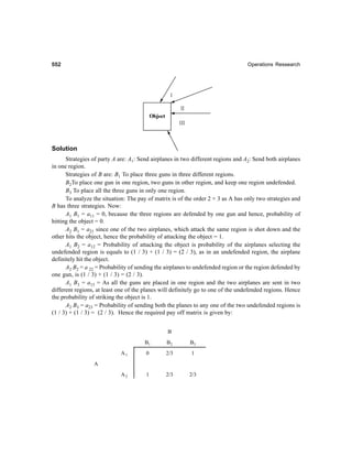


![Theory of Games or Competitive Stratagies 555
If A lets B win the first item, for Rs. x/-, then B will be left with Rs. (155 – x) only for bidding the
second item i.e. he cannot make a bid more than Rs. (155 – x) for the second item. Thus A will be
positively able to win the second item for Rs. (155 – x + λ ). Therefore, A’s gain by allowing B to win
the first item for Rs. x/- will be Rs. [150 – (155 – x + λ )] = (x – λ – 5).
On the other hand, if A bids Rs. (x + λ ), for the first item and B lets him to win the bid, then
A’s gain will be Rs. ([100 – (x + λ )] = (100 – x – λ ).
Now since A wants to maximize his return, he should bid Rs. (x + λ ) for the first item
provided (100 – x – λ ) ≥ (x – λ – 5) or x ≤ Rs. 52.50
Thus A should bid for first item until x ≤ Rs. 52.50. In case x > Rs. 5.50, he should allow B to
win the first item.
Similarly, B’s gains in the two alternatives are: Rs. [150 – (125 – y) – λ ] and Rs. (100 – y –
λ ), where y denote A’s bid for the firs item. Thus B should bid Rs. (y + λ ) for the first item
provided:
(100 – y – λ ) ≥ [150 – (125 – y) – λ ] or y ≤ Rs. 37.50
Obviously, A will win the fist item for Rs. 37.50 because he can increase his bid without any
loss up to Rs. 52.50, and B will get the second item for Rs. 125 – Rs. 37.50 = Rs. 87.50 because a,
after winning the first item in Rs. 37.50 cannot increase his bid for the second item beyond Rs.
87.50. Thus B will get the second item for Rs. 87.50. Therefore A’s gain is Rs. 100 – Rs.37.50 =
Rs. 62.50 and B’s gain is Rs. 250 – Rs. 87.50 = Rs. 62.50.
Problem 10.47.
Two items of values Rs.100/- and Rs. 120 respectively are to be bid simultaneously by two
bidders A and B. Both players intend to devote a lot of sum of Rs. 130 to the two bids. If each uses a
minimax criterion, find the resulting bids.
Solution
Here the bids are closed since they are to be made simultaneously. Let A1 and A2 are the A’s
optimum bids for the first and second items respectively. Obviously, A’s optimum bids are the ones
that fetch the same profit to A on both the items. If p denote the profit earned by the successful bid,
then,
2p = (100 – A1) + (120 – A2) or 2p = 220 – A1 – A2
Since both A and B intend to devote only Rs. 130/- for both the bids, A1 + A2 = Rs. 130/-
Therefore, 2p = Rs.(220 – 130) = Rs. 90/- or p = Rs. 45/-
Now p = 100 – A1 or A1 = 100 – p = 100 – 45 = Rs. 55/-
Also, p = 120 – A2 or A2 = 120 – p = 120 – 45 = RS. 75/-
Thus optimum bids for A are Rs. 55/- and Rs. 75/- for the first and second items respectively.
Likewise, optimum bids for B can be determined and will be Rs 55/- and Rs. 75/- respectively for the
two items.](https://image.slidesharecdn.com/operationsresearch-151024043006-lva1-app6892/85/Operations-research-566-320.jpg)


![558558558558558 Operations Ressearch
Value of game for B = [(2 / 4) – (3 / 4)] / [(1 / 4 + (3 / 4)] = – (1 / 4)
Value of game for A and C is (1 / 4)
3. C against A and B. Pay of matrix is:
A and B
X1 Y1 X1 Y2 X2 Y1 X2 Y2 Row minimum
Z1 –2 4 0 2 –2
C
Z2 1 –1 3 1 –1
Column Maximum: 1 4 3 2
The game has no saddle point. First column dominates third and fourth column. Hence the
reduced matrix is:
A and B
X1 Y1 X1 Y2 oddment Probability
Z1 –2 4 2 2 / 8
C
Z2 1 –1 6 6 / 8
Oddment 5 3
Probability. 5 / 8 3 / 8
C's best strategy is to play (Z1, Z2) = [(2 / 8), (6 / 8)]
For A and B = (X1 Y1, X1 Y2) = [(5 / 8), (3 / 8)]
Value of the game for C = [–(10 / 8) + (12 / 8)] / [(5 / 8) + (3 / 8)] = (2 / 8) / 1 = (1 / 4)
Value of the game for A and B is – (1 / 4) as this is a zero sum game.
Therefore, the characteristics of the game are:
V (A) = 0, V (B) = – (1 / 4), V (C) = (1 / 4) and V (B, C) = 0, V (A, C) = (1 / 4). V (A, B) = – (1
/ 4)
QUESTIONS
1. What are competitive situations? Explain with the help of an example.
2. What is a business game? Enlist the properties of the game. What assumptions are made in
game theory?
3. Explain Maximin and Minimax principle with respect to game theory.
4. By means of an example, explain what do you mean by Two Person Zero Sum game.
5. Solve the following game, whose pay of matrix is:](https://image.slidesharecdn.com/operationsresearch-151024043006-lva1-app6892/85/Operations-research-569-320.jpg)


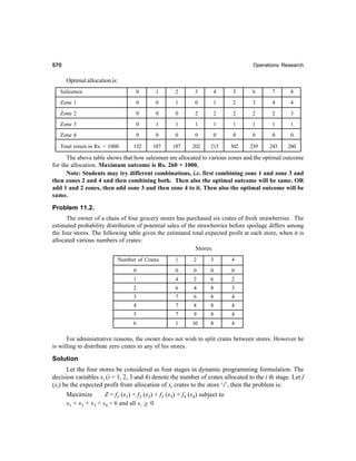


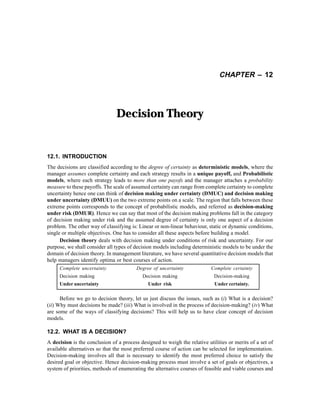


Operations research
- 5. Copyright © 2007, 2005 NewAge International (P) Ltd., Publishers Published by New Age International (P) Ltd., Publishers All rights reserved. No part of this ebook may be reproduced in any form, by photostat, microfilm, xerography, or any other means, or incorporated into any information retrieval system, electronic or mechanical, without the written permission of the publisher. All inquiries should be emailed to rights@newagepublishers.com ISBN (13) : 978-81-224-2944-2 PUBLISHING FOR ONE WORLD NEWAGE INTERNATIONAL(P) LIMITED, PUBLISHERS 4835/24,Ansari Road, Daryaganj, New Delhi - 110002 Visitusatwww.newagepublishers.com
- 6. PREFACE I started my teaching career in the year 1964. I was teaching Production Engineering subjects till 1972. In the year 1972 I have registered my name for the Industrial Engineering examination at National Institution of Industrial Engineering, Bombay. Since then, I have shifted my field for interest to Industrial Engineering subjects and started teaching related subjects. One such subject is OPERATIONS RESEARCH. After teaching these subjects till my retirement in the year 2002, it is my responsibility to help the students with a book on Operations research. The first volume of the book is LINEAR PORGRAMMING MODELS. This was published in the year 2003. Now I am giving this book OPERATIONS RESEARCH, with other chapters to students, with a hope that it will help them to understand the subject easily. I hope this will help my teacher friends to teach the subject well. I thank Mr. N.V. Jagdeesh Babu, Assistant professor of Mechanical Engineering for proof reading the script. Anantapur Date: 12.1.2007 P. Rama Murthy.
- 8. Dedicated To My Wife Usha My Daughter Vidya Grandson Yagnavalkya. and My Son In Law Shankaranarayana
- 10. CONTENTS Preface Chapter Title Page number 1. Historical Development............................................................................ 1-21 2. Linear Programming models (Resource allocation models) ................. 22-43 3. Linear Programming models (Solution by Simplex method) .............. 44-140 4. Linear Programming - II (Transportation Problem) ..........................141-211 5. Linear Programming III (Assignment Model) .................................. 212-254 6. Sequencing Model ............................................................................. 255-294 7. Replacement Model ........................................................................... 295-353 8. Inventory Control .............................................................................. 354-445 9. Waiting line theory or Queuing Model............................................... 446-484 10. Theory of Games or Competitive Strategies ..................................... 485-563 11. Dynamic Programming ..................................................................... 564-592 12. Decision Theory ................................................................................ 593-616 13. Simulation .......................................................................................... 617-626 14. Introduction to Non - Linear Programming ...................................... 627-634 15. Programme Evaluation and Review Technique and Critical Path Method (PERT AND CPM).......................................... 635-670 Multiple choice question and answers .......................................................... 671-702 Index ........................................................................................................... 703-705
- 12. 1.1. INTRODUCTION The subject OPERATIONS RESEARCH is a branch of mathematics - specially applied mathematics, used to provide a scientific base for management to take timely and effective decisions to their problems. It tries to avoid the dangers from taking decisions merely by guessing or by using thumb rules. Management is the multidimensional and dynamic concept. It is multidimensional, because management problems and their solutions have consequences in several dimensions, such as human, economic social and political fields. As the manager operates his system in an environment, which will never remain static, hence is dynamic in nature. Hence any manager, while making decisions, consider all aspects in addition to economic aspect, so that his solution should be useful in all aspects. The general approach is to analyse the problem in economic terms and then implement the solution if it does not aggressive or violent to other aspects like human, social and political constraints. Management may be considered as the process of integrating the efforts of a purposeful group, or organisation, whose members have at least one common goal. You have studied various schools of management in your management science. Most important among them which uses scientific basis for decision making are: (i) The Decision theory or Decisional Management School and (ii) The Mathematical or Quantitative Measurement School. The above-mentioned schools of management thought advocate the use of mathematical methods or quantitative methods for making decisions. Quantitative approach to management problems requires that decision problems be defined, analyzed, and solved in a conscious, rational, logical and systematic and scientific manner - based on data, facts, information and logic, and not on mere guess work or thumb rules. Here we use objectively measured decision criteria. Operations research is the body of knowledge, which uses mathematical techniques to solve management problems and make timely optimal decisions. Operations Research is concerned with helping managers and executives to make better decisions. Today’s manager is working in a highly competitive and dynamic environment. In present environment, the manager has to deal with systems with complex interrelationship of various factors among them as well as equally complicated dependence of the criterion of effective performance of the system on these factors, conventional methods of decision-making is found very much inadequate. Though the common sense, experience, and commitment of the manager is essential in making decision, we cannot deny the role-played by scientific methods in making optimal decisions. Operations Research CHAPTER – 1 Historical Development
- 13. 22222 Operations Research uses logical analysis and analytical techniques to study the behaviour of a system in relation to its overall working as resulting from its functionally interconnected constraints, whose parameters are recognized, quantified wherever possible relationships identified to the extent possible and alterative decisions are derived. Conventional managers were very much worried about that an Operations Research analyst replace them as a decision maker, but immediately they could appreciated him due to his mathematical and logical knowledge, which he applies while making decisions. But operations research analyst list out alternative solutions and their consequences to ease manager’s work of decision making. Operations research gives rationality to decision-making with clear view of possible consequences. The scope of quantitative methods is very broad. They are applied in defining the problems and getting solutions of various organisatons like, business, Government organisations, profit making units and non-profit units and service units. They can be applied to variety of problems like deciding plant location, Inventory control, Replacement problems, Production scheduling, return on investment analysis (ROI), Portfolio selection, marketing research and so on. This book, deals with basic models of Operations research and quantitative methods. The students have to go through advanced Operations Research books, to understand the scope of the subject. Two important aspects of quantitative methods are: (a) Availability of well-structured models and methods in solving the problems, (b) The attitude of search, conducted on a scientific basis, for increased knowledge in the management of organisations. Therefore, the attitude encompassed in the quantitative approaches is perhaps more important than the specific methods or techniques. It is only by adopting this attitude that the boundaries and application of the quantitative approach can be advanced to include those areas where, at first glance, quantitative data and facts are hard to come by. Hence, quantitative approach has found place in traditional business and as well in social problems, public policy, national, international problems and interpersonal problems. In fact we can say that the application of quantitative techniques is not limited to any area and can be conveniently applied to all walks of life as far as decision-making is concerned. The quantitative approach does not preclude the qualitative or judgemental elements that almost always exert a substantial influence on managerial decision-making. Quite the contrary. In actual practice, the quantitative approach must build upon, be modified by, and continually benefit from the experiences and creative insight of business managers. In fact quantitative approach imposes a special responsibility on the manager. It makes modern manager to cultivate a managerial style that demand conscious, systematic and scientific analysis - and resolution - of decision problems. In real world problems, we can notice that there exists a relationship among intuition, judgement, science, quantitative attitudes, practices, methods and models, as shown in figure 1.1. The figure depicts that higher the degree of complexity and the degree of turbulence in the environment, the greater is the importance of the qualitative approach to management. On the other hand, the lower the degree of complexity i.e., simple and well-structured problems, and lesser degree of turbulence in the environment, the greater is the potential of quantitative models. The advancement in quantitative approach to management problems is due to two facts. They are: (a) Research efforts have been and are being directed to discover and develop more efficient tools and techniques to solve decision problems of all types.
- 14. Historical Development 33333 (b) Through a continuous process of testing new frontiers, attempts have been made to expand the boundaries and application potential of the available techniques. Quantitative approach is assuming an increasing degree of importance in the theory and practice of management because of the following reasons. (a) Decision problems of modern management are so complex that only a conscious, systematic and scientifically based analysis can yield a realistic fruitful solution. (b) Availability of list of more potential models in solving complex managerial problems. (c) The most important one is that availability of high speed computers to solve large and complex real world problems in less time and at least cost and which help the managers to take timely decision. One thing we have to remember here is that if managers are to fully utilize the potentials of management science models and computers, then problems will have to be stated in quantitative terms. As far as the title of the subject is concerned, the terms ‘quantitative approach’, ‘operations research’, ‘management science’, ‘systems analysis’ and ‘systems science’ are often used interchangeably. What ever be the name of the subject, the syllabi and subject matter dealt which will be same. This analog to ‘god is one but the names are different’. Figure. 1.1. Qualitative Thinking and Quantitative models. 1.2. HISTORY OF OPERATIONS RESEARCH Operations Research is a ‘war baby’. It is because, the first problem attempted to solve in a systematic way was concerned with how to set the time fuse bomb to be dropped from an aircraft on to a submarine. In fact the main origin of Operations Research was during the Second World War. At Decision Process Turbulent and Differentiated Environment SCIENCEAND QUANTITATIVE MODELS Intuition Judgement Placid and Uniform Environment Complex and III-structured Problems Simple and Well-structured Problems Intelligence, Information and Data
- 15. 44444 Operations Research the time of Second World War, the military management in England invited a team of scientists to study the strategic and tactical problems related to air and land defense of the country. The problem attained importance because at that time the resources available with England was very limited and the objective was to win the war with available meager resources. The resources such as food, medicines, ammunition, manpower etc., were required to manage war and for the use of the population of the country. It was necessary to decide upon the most effective utilization of the available resources to achieve the objective. It was also necessary to utilize the military resources cautiously. Hence, the Generals of military, invited a team of experts in various walks of life such as scientists, doctors, mathematicians, business people, professors, engineers etc., and the problem of resource utilization is given to them to discuss and come out with a feasible solution. These specialists had a brain storming session and came out with a method of solving the problem, which they coined the name “Linear Programming”. This method worked out well in solving the war problem. As the name indicates, the word Operations is used to refer to the problems of military and the word Research is use for inventing new method. As this method of solving the problem was invented during the war period, the subject is given the name ‘OPERATIONS RESEARCH’ and abbreviated as ‘O.R.’ After the World War there was a scarcity of industrial material and industrial productivity reached the lowest level. Industrial recession was there and to solve the industrial problem the method linear programming was used to get optimal solution. From then on words, lot of work done in the field and today the subject of O.R. have numerous methods to solve different types of problems. After seeing the success of British military, the United States military management started applying the techniques to various activities to solve military, civil and industrial problems. They have given various names to this discipline. Some of them are Operational Analysis, Operations Evaluation, Operations Research, System Analysis, System Evaluation, Systems Research, Quantitative methods, Optimisation Techniques and Management Science etc. But most widely used one is OPERATIONS RESEARCH. In industrial world, most important problem for which these techniques used is how to optimise the profit or how to reduce the costs. The introduction of Linear Programming and Simplex method of solution developed by American Mathematician George B. Dontzig in 1947 given an opening to go for new techniques and applications through the efforts and co-operation of interested individuals in academic field and industrial field. Today the scenario is totally different. A large number of Operations Research consultants are available to deal with different types of problems. In India also, we have O.R. Society of India (1959) to help in solving various problems. Today the Operations Research techniques are taught at High School levels. To quote some Indian industries, which uses Operations Research for problem solving are: M/S Delhi Cloth Mills, Indian Railways, Indian Airline, Hindustan Lever, Tata Iron and Steel Company, Fertilizers Corporation of India and Defense Organizations. In all the above organizations, Operations Research people act as staff to support line managers in taking decisions. In one word we can say that Operations Research play a vital role in every organization, especially in decision-making process. 1.3. DECISION MAKING AND SOME ASPECTS OF DECISION Many a time we speak of the word decision, as if we know much about decision. But what is decision? What it consists of? What are its characteristics? Let us have brief discussion about the word decision, as much of our time we deal with decision-making process in Operations Research. A decision is the conclusion of a process designed to weigh the relative uses or utilities of a set of alternatives on hand, so that decision maker selects the best alternative which is best to his problem
- 16. Historical Development 55555 or situation and implement it. Decision Making involves all activities and thinking that are necessary to identify the most optimal or preferred choice among the available alternatives. The basic requirements of decision-making are (i) A set of goals or objectives, (ii) Methods of evaluating alternatives in an objective manner, (iii) A system of choice criteria and a method of projecting the repercussions of alternative choices of courses of action. The evaluation of consequences of each course of action is important due to sequential nature of decisions. The necessity of making decisions arises because of our existence in the world with various needs and ambitions and goals, whose resources are limited and some times scarce. Every one of us competes to use these resources to fulfill our goals. Our needs can be biological, physical, financial, social, ego or higher-level self-actualisation needs. One peculiar characteristics of decision-making is the inherent conflict that desists among various goals relevant to any decision situation (for example, a student thinking of study and get first division and at the same time have youth hood enjoyment without attending classes, OR a man wants to have lot of leisure in his life at the same time earn more etc.). The process of decision-making consists of two phases. The first phase consists of formulation of goals and objectives, enumeration of environmental constraints, identification and evaluation of alternatives. The second stage deals with selection of optimal course of action for a given set of constraints. In Operations Research, we are concerned with how to choose optimal strategy under specified set of assumptions, including all available strategies and their associated payoffs. Decisions may be classified in different ways, depending upon the criterion or the purpose of classification. Some of them are shown below: I Decisions (depending on the purpose) PURPOSE: Strategic Administrative Operational Related to external Resource utilisation of Related to day –to-day Environment an orgnisation. Repetitive work. II Decision (Depending on the nature) Programmed decisions Non Programmed decisions Meant for repetitive and well-structured Meant for non-routine, novel, problems. Inventory Problems, ill-structured problems. Policy matters, Product Mix Problems, etc. Product market mix, plant location Etc. III Decisions (Depending on the persons involved) Individual Managerial
- 17. 66666 Operations Research IV. Decisions (Depending on the Sphere of interest) Economic Social Business Political Social V. Decisions (depending on the time horizon) Static Dynamic (One decision for entire planning period) (Decisions are sequential) Decisions may also be classified depending on the situations such as degree of certainty. For example, (i) Decision making under certainty (ii) Decision making under Uncertainty and (iii) Decision making under risk. The first two are two extremes and the third one is falls between these two with certain probability distribution. Figure 1.2. Decision based on degree of certainty. 1.4. OBJECTIVE OF OPERATIONS RESEARCH Today’s situation in which a manager has to work is very complicated due to complexity in business organizations. Today’s business unit have number of departments and each department work for fulfilling the objectives of the organization. While doing so the individual objective of one of the department may be conflicting with the objective of the other department, though both working for achieving the common goal in the interest of the organization. In such situations, it will become a very complicated issue for the general manager to get harmony among the departments and to allocate the available resources of all sorts to the departments to achieve the goal of the organization. At the same time the
- 18. Historical Development 77777 environment in which the organization is operating is very dynamic in nature and the manager has to take decisions without delay to stand competitive in the market. At the same time a wrong decision or an untimely decision may be very costly. Hence the decision making process has become very complicated at the same time very important in the environment of conflicting interests and competitive strategies. Hence it is desirable for modern manager to use scientific methods with mathematical base while making decisions instead of depending on guesswork and thumb rule methods. Hence the knowledge of Operations Research is an essential tool for a manager who is involved in decision- making process. He must have support of knowledge of mathematics, statistics, economics etc., so that the decision he takes will be an optimal decision for his organisaton. Operation Research provides him this knowledge and helps him to take quick, timely, decisions, which are optimal for the organisaton. Hence the objective of operations research is: “The objective of Operations Research is to provide a scientific basis to the decision maker for solving the problems involving the interaction of various components of an organization by employing a team of scientists from various disciplines, all working together for finding a solution which is in the best interest of the organisaton as a whole. The best solution thus obtained is known as optimal decision”. 1.5. DEFINITION OF OPERATIONS RESEARCH Any subject matter when defined to explain what exactly it is, we may find one definition. Always a definition explains what that particular subject matter is. Say for example, if a question is asked what is Boyel's law, we have a single definition to explain the same, irrespective of the language in which it is defined. But if you ask, what Operations research is? The answer depends on individual objective. Say for example a student may say that the Operations research is technique used to obtain first class marks in the examination. If you ask a businessman the same question, he may say that it is the technique used for getting higher profits. Another businessman may say it is the technique used to capture higher market share and so on. Like this each individual may define in his own way depending on his objective. Each and every definition may explain one or another characteristic of Operations Research but none of them explain or give a complete picture of Operations research. But in the academic interest some of the important definitions are discussed below. (a) Operations Research is the art of winning wars without actually fighting. - Aurther Clarke. This definition does not throw any light on the subject matter, but it is oriented towards warfare. It means to say that the directions for fighting are planned and guidance is given from remote area, according to which the war is fought and won. Perhaps you might have read in Mahabharatha or you might have seen some old pictures, where two armies are fighting, for whom the guidance is given by the chief minister and the king with a chessboard in front of them. Accordingly war is fought in the warfront. Actually the chessboard is a model of war field. (b) Operations Research is the art of giving bad answers to problems where otherwise worse answers are given. - T.L. Satty. This definition covers one aspect of decision-making, i.e., choosing the best alternative among the list of available alternatives. It says that if the decisions are made on guesswork, we may face the worse situation. But if the decisions are made on scientific basis, it will help us to make better decisions. Hence this definition deals with one aspect of decision-making and not clearly tells what is operations research.
- 19. 88888 Operations Research (c) Operations Research is Research into Operations. - J. Steinhardt. This definition does not give anything in clear about the subject of Operations Research and simply says that it is research in to operations. Operations may here be referred as military activities or simply the operations that an executive performs in his organisations while taking decisions. Research in the word means that finding a new approach. That is when an executive is involved in performing his operations for taking decisions he has to go for newer ways so that he can make a better decision for the benefit of his organisation. (d) Operations Research is defined as Scientific method for providing executive departments a quantitative basis for decisions regarding the operations under their control. - P.M. Morse and G.E. Kimball. This definition suggests that the Operations Research provides scientific methods for an executive to make optimal decisions. But does not give any information about various models or methods. But this suggests that executives can use scientific methods for decision-making. (e) Operations Research is th study of administrative system pursued in the same scientific manner in which system in Physics, Chemistry and Biology are studied in natural sciences. This definition is more elaborate than the above given definitions. It compares the subject Operations Research with that of natural science subjects such as Physics, Chemistry and Biology, where while deciding any thing experiments are conducted and results are verified and then the course of action is decided. It clearly directs that Operations Research can also be considered as applied science and before the course of action is decided, the alternatives available are subjected to scientific analysis and optimal alternative is selected. But the difference between the experiments we conduct in natural sciences and operations research is: in natural sciences the research is rigorous and exact in nature, whereas in operations research, because of involvement of human element and uncertainty the approach will be totally different. (f) Operations Research is the application of scientific methods, techniques and tools to operation of a system with optimum solution to the problem. - Churchman, Ackoff and Arnoff. This definition clearly states that the operations research applies scientific methods to find an optimum solution to the problem of a system. A system may be a production system or information system or any system, which involves men, machine and other resources. We can clearly identify that this definition tackles three important aspects of operations research i.e. application of scientific methods, study of a system and optimal solution. This definition too does not give any idea about the characteristics of operations research. (g) Operations Research is the application of the theories of Probability, Statistics, Queuing, Games, Linear Programming etc., to the problems of War, Government and Industry. This definition gives a list of various techniques used in Operations Research by various managers to solve the problems under their control. A manager has to study the problem, formulate the problem, identify the variables and formulate a model and select an appropriate technique to get optimal solution. We can say that operations research is a bunch of mathematical techniques to solve problems of a system. (h) Operations Research is the use of Scientific Methods to provide criteria or decisions regarding man-machine systems involving repetitive operations.
- 20. Historical Development 99999 This definition talks about man- machine system and use of scientific methods and decision- making. It is more general and comprehensive and exhaustive than other definitions. Wherever a study of system involving man and machine, the person in charge of the system and involved in decision-making will use scientific methods to make optimal decisions. (i) Operations Research is applied decision theory. It uses any scientific, mathematical or logical means to attempt to cope with problems that confront the executive, when he tries to achieve a thorough going rationally in dealing with his decision problem. - D.W. Miller and M.K. Starr. This definition also explains that operations research uses scientific methods or logical means for getting solutions to the executive problems. It too does not give the characteristics of Operations Research. (j) Operations Research is the application of the methods of science to complex problems arising in the direction and management of large systems of men, materials and money in industry, business, Government and defense. The distinctive approach is to develop a scientific model of the system, incorporating measurements of factors such as chance and risk, with which to predict and compare the outcome of alternative decisions, strategies or controls. The purpose is to help management to determine its policy and actions scientifically. - Operations Society of Great Britain. The above definition is more elaborate and says that operations research applies scientific methods to deal with the problems of a system where men, material and other resources are involved and the system under study may be industry, defense or business etc, gives this definition. It also say that the manager has to build a scientific model to study the system which must be provided with facility to measure the outcomes of various alternatives under various degrees of risk, which helps the managers to take optimal decisions. In addition to the above there are hundreds of definitions available to explain what Operations Research is? But many of them are not satisfactory because of the following reasons. (i) Operations Research is not a well-defined science like Physics, Chemistry etc. All these sciences are having well defined theory about the subject matter, where as operations research do not claim to know or have theories about operations. Moreover, Operations Research is not a scientific research into the control of operations. It is only the application of mathematical models or logical analysis to the problem solving. Hence none of the definitions given above defines operations research precisely. (ii) The objective of operations research says that the decisions are made by brain storming of people from various walks of life. This indicates that operations research approach is inter- disciplinary approach, which is an important character of operations research. This aspect is not included in any of the definitions hence they are not satisfactory. (iii) The above-discussed definitions are given by various people at different times and stages of development of operations research as such they have considered the field in which they are involved hence each definition is concentrating on one or two aspects. No definition is having universal approach. But salient features of above said definitions are: * Operations Research uses Scientific Methods for making decisions. * It is interdisciplinary approach for solving problems and it uses the knowledge and experience of experts in various fields.
- 21. 1010101010 Operations Research * While analyzing the problems all aspects are considered and examined and analyzed scientifically for finding the optimal solution for the problem on hand. * As operations research has scientific approach, it improves the quality of answers to the problems. * Operations research provides scientific base for decision-making and provide scientific substitute for judgement and intuition. 1.6. CHARACTERISTICS OF OPERATIONS RESEARCH After considering the objective and definitions of Operations Research, now let us try to understand what are the characteristics of Operations Research. (a) Operations Research is an interdisciplinary team approach. The problems an operations research analyst face is heterogeneous in nature, involving the number of variables and constraints, which are beyond the analytical ability of one person. Hence people from various disciplines are required to understand the operations research problem, who applies their special knowledge acquired through experience to get a better view of cause and effects of the events in the problem and to get a better solution to the problem on hand. This type of team approach will reduce the risk of making wrong decisions. (b) Operations Research increases the creative ability of the decision maker. Operations Research provides manager mathematical tools, techniques and various models to analyse the problem on hand and to evaluate the outcomes of various alternatives and make an optimal choice. This will definitely helps him in making better and quick decisions. A manager, without the knowledge of these techniques has to make decisions by thumb rules or by guess work, which may click some times and many a time put him in trouble. Hence, a manager who uses Operations Research techniques will have a better creative ability than a manager who does not use the techniques. (c) Operations Research is a systems approach. A business or a Government organization or a defense organization may be considered as a system having various sub-systems. The decision made by any sub-system will have its effect on other sub-systems. Say for example, a decision taken by marketing department will have its effect on production department. When dealing with Operations Research problems, one has to consider the entire system, and characteristics or sub- systems, the inter-relationship between sub-systems and then analyse the problem, search for a suitable model and get the solution for the problem. Hence we say Operations Research is a Systems Approach. 1.7. SCOPE OF OPERATIONS RESEARCH The scope aspect of any subject indicates, the limit of application of the subject matter/techniques of the subject to the various fields to solve the variety of the problems. But we have studied in the objective, that the subject Operations Research will give scientific base for the executives to take decisions or to solve the problems of the systems under their control. The system may be business, industry, government or defense. Not only this, but the definitions discussed also gives different versions. This indicates that the techniques of Operations Research may be used to solve any type of problems. The problems may pertain to an individual, group of individuals, business, agriculture, government or
- 22. Historical Development 1111111111 defense. Hence, we can say that there is no limit for the application of Operations Research methods and techniques; they may be applied to any type of problems. Let us now discuss some of the fields where Operations Research techniques can be applied to understand how the techniques are useful to solve the problems. In general we can state that whenever there is a problem, simple or complicated, we can use operations research techniques to get best solution. (i) In Defense Operations In fact, the subject Operations research is the baby of World War II. To solve war problems, they have applied team approach, and come out with various models such as resource allocation model, transportation model etc.In any war field two or more parties are involved, each having different resources (manpower, ammunition, etc.), different courses of actions (strategies) for application. Every opponent has to guess the resources with the enemy, and his courses of action and accordingly he has to attack the enemy. For this he needs scientific, logical analysis of the problem to get fruitful results. Here one can apply the techniques like Linear Programming, Game theory, and inventory models etc. to win the game. In fact in war filed every situation is a competitive situation. More over each party may have different bases, such as Air force, Navy and Army. The decision taken by one will have its effect on the other. Hence proper co-ordination of the three bases and smooth flow of information is necessary. Here operations research techniques will help the departmental heads to take appropriate decisions. (ii) In Industry After the II World War, the, Industrial world faced a depression and to solve the various industrial problems, industrialist tried the models, which were successful in solving their problems. Industrialist learnt that the techniques of operations research can conveniently applied to solve industrial problems. Then onwards, various models have been developed to solve industrial problems. Today the managers have on their hand numerous techniques to solve different types of industrial problems. In fact decision trees, inventory model, Linear Programming model, Transportation model, Sequencing model, Assignment model and replacement models are helpful to the managers to solve various problems, they face in their day to day work. These models are used to minimize the cost of production, increase the productivity and use the available resources carefully and for healthy industrial growth. An industrial manager, with these various models on his hand and a computer to workout the solutions (today various packages are available to solve different industrial problems) quickly and preciously. (iii) In Planning For Economic Growth In India we have five year planning for steady economic growth. Every state government has to prepare plans for balanced growth of the state. Various secretaries belonging to different departments has to co-ordinate and plan for steady economic growth. For this all departments can use Operations research techniques for planning purpose. The question like how many engineers, doctors, software people etc. are required in future and what should be their quality to face the then problems etc. can be easily solved. (iv) In Agriculture The demand for food products is increasing day by day due to population explosion. But the land available for agriculture is limited. We must find newer ways of increasing agriculture yield. So the selection of land area for agriculture and the seed of food grains for sowing
- 23. 1212121212 Operations Research must be meticulously done so that the farmer will not get loss at the same time the users will get what they desire at the desired time and desired cost. (v) In Traffic control Due to population explosion, the increase in the number and verities of vehicles, road density is continuously increasing. Especially in peak hours, it will be a headache to control the traffic. Hence proper timing of traffic signaling is necessary. Depending on the flow of commuters, proper signaling time is to be worked out. This can be easily done by the application of queuing theory. (vi) In Hospitals Many a time we see very lengthy queues of patient near hospitals and few of them get treatment and rest of them have to go without treatment because of time factor. Some times we have problems non-availability of essential drugs, shortage of ambulances, shortage of beds etc. These problems can be conveniently solved by the application of operations research techniques. The above-discussed problems are few among many problems that can be solved by the application of operation research techniques. This shows that Operations Research has no limit on its scope of application. 1.8. PHASES IN SOLVING OPERATIONS RESEARCH PROBLEMS OR STEPS IN SOLVING OPERATIONS RESEARCH PROBLEMS Any Operations Research analyst has to follow certain sequential steps to solve the problem on hand. The steps he has to follow are discussed below: First he has to study the situation and collect all information and formulate the statement of the problem. Hence the first step is the Formulation of the problem. The figure 1.3 shows the various steps to be followed. 1.8.1. Formulation of the Problem The Operations Research analyst or team of experts first have to examine the situation and clearly define what exactly happening there and identify the variables and constraints. Similarly identify what is the objective and put them all in the form of statement. The statement must include a) a precise description goals or objectives of the study, b) identification of controllable and uncontrollable variables and c) restrictions of the problem. The team should consult the personals at the spot and collect information, if something is beyond their reach, they have to consult duty engineers available and understand the facts and formulate the problem. Let us consider the following statement: Statement: A company manufactures two products X and Y, by using the three machines A, B, and C. Each unit of X takes 1 hour on machine A, 3 hours on machine B and 10 hours on machine C. Similarly, product Y takes one hour, 8 hours and 7 hours on Machine A, B, and C respectively. In the coming planning period, 40 hours of machine A, 240 hours of machine B and 350 hours of machine C is available for production. Each unit of X brings a profit of Rs 5/- and Y brings Rs. 7 per unit. How much of X and Y are to be manufactured by the company for maximizing the profit? The team of specialists prepares this statement after studying the system. As per requirement this must include the variables, constraints, and objective function.
- 24. Historical Development 1313131313 Figure 1.3. Phases of Solving Operations Research Problems. 1.8.2. Variables The Company is manufacturing two products X and Y. These are the two variables in the problem. When they are in the problem statement they are written in capital letters. Once they are entered in the model small letters (lower case) letters are used (i.e,. x and y). We have to find out how much of X and how much of Y are to be manufactured. Hence they are variables. In linear programming language, these are known as competing candidates. Because they compete to use or consume available resources. 1.8.3. Resources and Constraints There are three machines A, B, and C on which the products are manufactured. These are known as resources. The capacity of machines in terms of machine hours available is the available resources. The competing candidates have to use these available resources, which are limited in nature. Now in the above statement, machine A has got available 40 hours and machine B has available a capacity of 240 hours and that of machine C is 350 hours. The products have to use these machine hours in required proportion. That is one unit of product X consumes one hour of machine A, 3 hours of machine B and 10 hours of machine C. Similarly, one unit of Y consumes one hour of machine B, 8 hours of machine B and 7 hours of machine C. These machine hours given are the available resources and they are limited in nature and hence they are constraints given in the statement.
- 25. 1414141414 Operations Research 1.8.4. Objective of the Problem To maximise the profit how much of X and Y are to be manufactured? That is maximization of the profit or maximization of the returns is the objective of the problem. For this in the statement it is given that the profit contribution of X is Rs 5/- per unit and that of product Y is Rs. 7/- per unit. 1.8.5. To establish relationship between variables and constraints and build up a model Let us say that company manufactures x units of X and y units of Y. Then as one unit of x consumes one hour on machine A and one unit of y consumes one hour on machine A, the total consumption by manufacturing x units of X and y units of Y is, 1x + 1y and this should not exceed available capacity of 40 hours. Hence the mathematical relationship in the form of mathematical model is 1x + 1y ≤ 40. This is for resource machine A. Similarly for machine B and machine C we can formulate the mathematical models. They appear as shown below: 3x + 8y ≤ 240 for machine B and 10x + 7y ≤ 350 for machine C. Therefore, the mathematical model for these resources are: 1x + 1y ≤ 40 3x + 8y ≤ 240 and 10x + 7y ≤ 350. Similarly for objective function as the company manufacturing x units of X and y units of Y and the profit contribution of X and Y are Rs.5/- and Rs 7/- per unit of X and Y respectively, the total profit earned by the company by manufacturing x and y units is 5x + 7y. This we have to maximise. There- fore objective function is Maximise 5x + 7y. At the same time, we have to remember one thing that the company can manufacture any number of units or it may not manufacture a particular product, for example say x = 0. But it cannot manufacture negative units of x and y. Hence one more constraint is to be introduced in the model i.e. a non - negativity constraint. Hence the mathematical representation of the contents of the statement is as given below: Maximise Z = 5x + 7y Subject to a condition (written as s.t.) OBJECTIVE FUNCTION. 1x + 1y ≤ 40 3x + 8y ≤ 240 STRUCTURAL CONSTRAINTS. 10x + 7y ≤ 350 and Both x and y are ≥ 0 NON-NEGATIVITY CONSTRAINT. 1.8.6. Identify the possible alternative solutions (or known as Basic Feasible Solutions or simply BFS) There are various methods of getting solutions. These methods will be discussed later. For example we go on giving various values (positive numbers only), and find various values of objective function. All these are various Basic Feasible Solutions. For example x = 0,1,2,3, etc. and y = 0,1,2,3 etc are all feasible values as far as the given condition is concerned. Once we have feasible solutions on hand go on asking is it maximum? Once we get maximum value, those values of x and y are optimal values. And the value of objective function is optimal value of the objective function. These two steps we shall discuss in detail in the next chapter.
- 26. Historical Development 1515151515 1.8.7. Install and Maintain the Solution Once we get the optimal values of x and y and objective function instructions are given to the concerned personal to manufacture the products as per the optimal solution, and maintain the same until further instructions. 1.9. MEANING AND NECESSITY OF OPERATIONS RESEARCH MODELS Management deals with reality that is at once complex, dynamic, and multifacet. It is neither possible nor desirable, to consider each and every element of reality before deciding the courses of action. It is impossible because of time available to decide the courses of action and the resources, which are limited in nature. More over in many cases, it will be impossible for a manager to conduct experiment in real environment. For example, if an engineer wants to measure the inflow of water in to a reservoir through a canal, he cannot sit on the banks of canal and conduct experiment to measure flow. He constructs a similar model in laboratory and studies the problem and decides the inflow of water. Hence for many practical problems, a model is necessary. We can define an operations research model as some sort of mathematical or theoretical description of various variables of a system representing some aspects of a problem on some subject of interest or inquiry. The model enables to conduct a number of experiment involving theoretical subjective manipulations to find some optimum solution to the problem on hand. Let us take a very simple example. Say you have a small child in your house. You want to explain to it what is an elephant. You can say a story about the elephant saying that it has a trunk, large ears, small eyes etc. The child cannot understand or remember anything. But if you draw small drawing of elephant on a paper and show the trunk, ears, eyes and it will grasp very easily the details of elephant. When a circus company comes to your city and take elephants in procession, then the child if observe the procession, it will immediately recognize the elephant. This is the exact use of a model. In your classrooms your teacher will explain various aspects of the subject by drawing neat sketches on the black board. You will understand very easily and when you come across real world system, you can apply what all you learnt in your classroom. Hence through a model, we can explain the aspect of the subject / problem / system. The inequalities given in section 1.8.5 is a mathematical model, which explains clearly the manufacturing system, given in section 1.8.1. (Here we can say a model is a relationship among specified variables and parameters of the system). 1.9.1. Classification of Models The models we use in operations research may broadly classified as: (i) Mathematical and Descriptive models, and (ii) Static and Dynamic Models. Mathematical and Descriptive Models (i) Descriptive Model A descriptive model explains or gives a description of the system giving various variables, constraints and objective of the system or problem. In article 1.8.1 gives the statement of the problem, which is exactly a descriptive model. The drawback of this model is as we go on reading and proceed; it is very difficult to remember about the variables and constraints, in case the problem or description of the system is lengthy one. It is practically impossible to keep on reading, as the manager has to decide the course of action to be taken timely.
- 27. 1616161616 Operations Research Hence these models, though necessary to understand the system, have limited use as far as operations research is concerned. (ii) Mathematical Model In article, 1.8.2 we have identified the variables and constraints and objective in the problem statement and given them mathematical symbols x and y and a model is built in the form of an inequality of ≤ type. Objective function is also given. This is exactly a mathematical model, which explains the entire system in mathematical language, and enables the operations research person to proceed towards solution. 1.9.2. Types of Models Models are also categorized depending on the structure, purpose, nature of environment, behaviour, by method of solution and by use of digital computers. (a) Classification by Structure (i) Iconic Models: These models are scaled version of the actual object. For example a toy of a car is an iconic model of a real car. In your laboratory, you might have seen Internal Combustion Engine models, Boiler models etc. All these are iconic models of actual engine and boiler etc. They explain all the features of the actual object. In fact a globe is an iconic model of the earth. These models may be of enlarged version or reduced version. Big objects are scaled down (reduced version) and small objects, when we want to show the features, it is scaled up to a bigger version. In fact it is a descriptive model giving the description of various aspects of real object. As far as operations research is concerned, is of less use. The advantages of these models: are It is easy to work with an iconic model in some cases, these are easy to construct and these are useful in describing static or dynamic phenomenon at some definite time. The limitations are, we cannot study the changes in the operation of the system. For some type of systems, the model building is very costly. It will be sometimes very difficult to carry out experimental analysis on these models. (ii) Analogue Model: In this model one set of properties are used to represent another set of properties. Say for example, blue colour generally represents water. Whenever we want to show water source on a map it is represented by blue colour. Contour lines on the map is also analog model. Many a time we represent various aspects on graph by defferent colours or different lines all these are analog models. These are also not much used in operations research. The best examples are warehousing problems and layout problems. (iii) Symbolic Models or Mathematical Models: In these models the variables of a problem is represented by mathematical symbols, letters etc. To show the relationships between variables and constraints we use mathematical symbols. Hence these are known as symbolic models or mathematical models. These models are used very much in operations research. Examples of such models are Resource allocation model, Newspaper boy problem, transportation model etc. (b) Classification by utility Depending on the use of the model or purpose of the model, the models are classified as Descriptive, Predictive and Prescriptive models.
- 28. Historical Development 1717171717 (i) Descriptive model: The descriptive model simply explains certain aspects of the problem or situation or a system so that the user can make use for his analysis. It will not give full details and clear picture of the problem for the sake of scientific analysis. (ii) Predictive model: These models basing on the data collected, can predict the approximate results of the situation under question. For example, basing on your performance in the examination and the discussions you have with your friends after the examination and by verification of answers of numerical examples, you can predict your score or results. This is one type of predictive model. (iii) Prescriptive models: We have seen that predictive models predict the approximate results. But if the predictions of these models are successful, then it can be used conveniently to prescribe the courses of action to be taken. In such case we call it as Prescriptive model. Prescriptive models prescribe the courses of action to be taken by the manager to achieve the desired goal. (c) Classification by nature of environment Depending on the environment in which the problem exists and the decisions are made, and depending on the conditions of variables, the models may be categorized as Deterministic models and Probabilistic models. (i) Deterministic Models: In this model the operations research analyst assumes complete certainty about the values of the variables and the available resources and expects that they do not change during the planning horizon. All these are deterministic models and do not contain the element of uncertainty or probability. The problems we see in Linear Programming, assumes certainty regarding the values of variables and constraints hence the Linear Programming model is a Deterministic model. (ii) Probabilistic or Stochastic Models: In these models, the values of variables, the pay offs of a certain course of action cannot be predicted accurately because of element of probability. It takes into consideration element of risk into consideration. The degree of certainty varies from situation to situation. A good example of this is the sale of insurance policies by Life Insurance Companies to its customers. Here the failure of life is highly probabilistic in nature. The models in which the pattern of events has been compiled in the form of probability distributions are known as Probabilistic or Stochastic Models. (d) Classification depending on the behaviour of the problem variables Depending on the behaviour of the variables and constraints of the problem they may be classified as Static Models or Dynamic models. (i) Static Models: These models assumes that no changes in the values of variables given in the problem for the given planning horizon due to any change in the environment or conditions of the system. All the values given are independent of the time. Mostly, in static models, one decision is desirable for the given planning period. (ii) Dynamic Models: In these models the values of given variables goes on changing with time or change in environment or change in the conditions of the given system. Generally, the dynamic models then exist a series of interdependent decisions during the planning period. (e) Classification depending on the method of getting the solution We may use different methods for getting the solution for a given model. Depending on these methods, the models are classified as Analytical Models and Simulation Models.
- 29. 1818181818 Operations Research (i) Analytical Models: The given model will have a well-defined mathematical structure and can be solved by the application of mathematical techniques. We see in our discussion that the Resource allocation model, Transportation model, Assignment model, Sequencing model etc. have well defined mathematical structure and can be solved by different mathematical techniques. For example, Resource allocation model can be solved by Graphical method or by Simplex method depending on the number of variables involved in the problem. All models having mathematical structure and can be solved by mathematical methods are known as Analytical Models. (ii) Simulation Models: The meaning of simulation is imitation. These models have mathematical structure but cannot be solved by using mathematical techniques. It needs certain experimental analysis. To study the behaviour of the system, we use random numbers. More complex systems can be studied by simulation. Studying the behaviour of laboratory model, we can evaluate the required values in the system. Only disadvantage of this method is that it does not have general solution method. 1.9.3. Some of the Points to be Remembered while Building a Model * When we can solve the situation with a simple model, do not try to build a complicated model. * Build a model that can be easily fit in the techniques available. Do not try to search for a technique, which suit your model. * In order to avoid complications while solving the problem, the fabrication stage of modeling must be conducted rigorously. * Before implementing the model, it should be validated / tested properly. * Use the model for which it is deduced. Do not use the model for the purpose for which it is not meant. * Without having a clear idea for which the model is built do not use it. It is better before using the model; you consult an operations research analyst and take his guidance. * Models cannot replace decision makers. It can guide them but it cannot make decisions. Do not be under the impression, that a model solves every type of problem. * The model should be as accurate as possible. * A model should be as simple as possible. * Benefits of model are always associated with the process by which it is developed. 1.9.4. Advantages of a Good Model (i) A model provides logical and systematic approach to the problem. (ii) It provides the analyst a base for understanding the problem and think of methods of solving. (iii) The model will avoid the duplication work in solving the problem. (iv) Models fix the limitation and scope of an activity. (v) Models help the analyst to find newer ways of solving the problem. (vi) Models saves resources like money, time etc. (vii) Model helps analyst to make complexities of a real environment simple.
- 30. Historical Development 1919191919 (viii) Risk of tampering the real object is reduced, when a model of the real system is subjected to experimental analysis. (ix) Models provide distilled economic descriptions and explanations of the operation of the system they represent. 1.9.5. Limitations of a Model (i) Models are constructed only to understand the problem and attempt to solve the problem; they are not to be considered as real problem or system. (ii) The validity of any model can be verified by conducting the experimental analysis and with relevant data characteristics. 1.9.6. Characteristics of a Good Model (i) The number of parameters considered in a model should be less to understand the problem easily. (ii) A good model should be flexible to accommodate any necessary information during the stages of building the model. (iii) A model must take less time to construct. (iv) A model may be accompanied by lower and upper bounds of parametric values. 1.9.7. Steps in Constructing a Model (i) Problem environment analysis and formulation: One has to study the system in all aspects, if necessary make relevant assumptions, have the decision for which he is constructing the model in mind and formulate the model. (ii) Model construction and assumptions: Identify the main variables and constraints and relate them logically to arrive at a model. (iii) Testing the model: After the formulation, before using check the model for its validity. 1.10. Methods of Solving Operations Research Problems There are three methods of solving an operations research problem. They are: (i) Analytical method, (ii) Iterative Method, (iii) The Monte-Carlo Technique. (i) Analytical Method: When we use mathematical techniques such as differential calculus, probability theory etc. to find the solution of a given operations research model, the method of solving is known as analytical method and the solution is known as analytical solution. Examples are problems of inventory models. This method evaluates alternative policies efficiently. (ii) Iterative Method (Numerical Methods): This is trial and error method. When we have large number of variables, and we cannot use classical methods successfully, we use iterative process. First, we set a trial solution and then go on changing the solution under a given set of conditions, until no more modification is possible. The characteristics of this method is that the trial and error method used is laborious, tedious, time consuming and costly. The solution we get may not be accurate one and is approximate one. Many a time we find that
- 31. 2020202020 Operations Research after certain number of iterations, the solution cannot be improved and we have to accept it as the expected optimal solution. (iii) Monte-Carlo Method: This method is based on random sampling of variable's values from a distribution of the variable. This uses sampling technique. A table of random numbers must be available to solve the problems. In fact it is a simulation process. 1.11. SOME IMPORTANT MODELS (PROBLEMS) WE COME ACROSS IN THE STUDY OF OPERATIONS RESEARCH 1. Linear Programming Model This model is used for resource allocation when the resources are limited and there are number of competing candidates for the use of resources. The model may be used to maximise the returns or minimise the costs. Consider the following two situations: (a) A company which is manufacturing variety of products by using available resources, want to use resources optimally and manufacture different quantities of each type of product, which yield different returns, so as to maximise the returns. (b) A company manufactures different types of alloys by purchasing the three basic materials and it want to maintain a definite percentage of basic materials in each alloy. The basic materials are to be purchased from the sellers and mix them to produce the desired alloy. This is to be done at minimum cost. Both of them are resource allocation models, the case (a) is maximisation problem and the case (b) is minimisation problem. (c) Number of factories are manufacturing the same commodities in different capacities and the commodity is sent to various markets for meeting the demands of the consumers, when the cost of transportation is known, the linear programming helps us to formulate a programme to distribute the commodity from factories to markets at minimum cost. The model used is transportation model. (d) When a company has number of orders on its schedule, which are to be processed on same machines and the processing time, is known, then we have to allocate the jobs or orders to the machines, so as to complete all the jobs in minimum time. This we can solve by using Assignment model. All the above-discussed models are Linear Programming Models. They can be solved by application of appropriate models, which are linear programming models. 2. Sequencing Model When a manufacturing firm has some job orders, which can be processed on two or three machines and the processing times of each job on each machine is known, then the problem of processing in a sequence to minimise the cost or time is known as Sequencing model. 3. Waiting Line Model or Queuing Model A model used for solving a problem where certain service facilities have to provide service to its customers, so as to avoid lengthy waiting line or queue, so that customers will get satisfaction from effective service and idle time of service facilities are minimised is waiting line model or queuing model.
- 32. Historical Development 2121212121 4. Replacement Model Any capital item, which is continuously used for providing service or for producing the product is subjected to wear and tear due to usage, and its efficiency goes on reducing. This reduction in efficiency can be predicted by the increasing number of breakdowns or reduced productivity. The worn out parts or components are to be replaced to bring the machine back to work. This action is known as maintenance. A time is reached when the maintenance cost becomes very high and the manager feels to replace the old machine by new one. This type of problems known as replacement problems and can be solved by replacement models. 5. Inventory Models Any manufacturing firm has to maintain stock of materials for its use. This stock of materials, which are maintained in stores, is known as inventory. Inventory is one form of capital or money. The company has to maintain inventory at optimal cost. There are different types of inventory problems, depending the availability and demand pattern of the materials. These can be solved by the application of inventory models. In fact depending on the number of variables, characteristics of variables, and the nature of constraints different models are available. These models, we study when we go chapter wise. QUESTIONS 1. Trace the history of Operations Research. 2. Give a brief account of history of Operations Research. 3. Discuss the objective of Operations Research. 4. "Operations Research is a bunch of mathematical techniques to break industrial problems”. Critically comment. 5. What is a Operations Research model? Discuss the advantages of limitation of good Operations Research model. 6. Discuss three Operations Research models. 7. What is a decision and what are its characteristics. 8. Briefly explain the characteristics of Operations Research. 9. Discuss the various steps used in solving Operations Research problems. 10. Discuss the scope of Operations Research.
- 33. 2.1. INTRODUCTION A model, which is used for optimum allocation of scarce or limited resources to competing products or activities under such assumptions as certainty, linearity, fixed technology, and constant profit per unit, is linear programming. Linear Programming is one of the most versatile, powerful and useful techniques for making managerial decisions. Linear programming technique may be used for solving broad range of problems arising in business, government, industry, hospitals, libraries, etc. Whenever we want to allocate the available limited resources for various competing activities for achieving our desired objective, the technique that helps us is LINEAR PROGRAMMING. As a decision making tool, it has demonstrated its value in various fields such as production, finance, marketing, research and development and personnel management. Determination of optimal product mix (a combination of products, which gives maximum profit), transportation schedules, Assignment problem and many more. In this chapter, let us discuss about various types of linear programming models. 2.2. PROPERTIES OF LINEAR PROGRAMMING MODEL Any linear programming model (problem) must have the following properties: (a) The relationship between variables and constraints must be linear. (b) The model must have an objective function. (c) The model must have structural constraints. (d) The model must have non-negativity constraint. Let us consider a product mix problem and see the applicability of the above properties. Example 2.1. A company manufactures two products X and Y, which require, the following resources. The resources are the capacities machine M1, M2, and M3. The available capacities are 50,25,and 15 hours respectively in the planning period. Product X requires 1 hour of machine M2 and 1 hour of machine M3. Product Y requires 2 hours of machine M1, 2 hours of machine M2 and 1 hour of machine M3. The profit contribution of products X and Y are Rs.5/- and Rs.4/- respectively. CHAPTER – 2 Linear Programming Models (Resource Allocation Models)
- 34. Linear Programming Models (Resource Allocation Models) 2323232323 The contents of the statement of the problem can be summarized as follows: Machines Products Availability in hours X Y M1 0 2 50 M2 1 2 25 M3 1 1 15 Profit in Rs. Per unit 5 4 In the above problem, Products X and Y are competing candidates or variables. Machine capacities are available resources. Profit contribution of products X and Y are given. Now let us formulate the model. Let the company manufactures x units of X and y units of Y. As the profit contributions of X and Y are Rs.5/- and Rs. 4/- respectively. The objective of the problem is to maximize the profit Z, hence objective function is: Maximize Z = 5x + 4y OBJECTIVE FUNCTION. This should be done so that the utilization of machine hours by products x and y should not exceed the available capacity. This can be shown as follows: For Machine M1 0x + 2y ≤ 50 For Machine M2 1x + 2y ≤ 25 and LINEAR STRUCTURAL CONSTRAINTS. For machine M3 1x + 1y ≤ 15 But the company can stop production of x and y or can manufacture any amount of x and y. It cannot manufacture negative quantities of x and y. Hence we have write, Both x and y are ≥ 0 . NON -NEGATIVITY CONSTRAINT. As the problem has got objective function, structural constraints, and non-negativity constraints and there exist a linear relationship between the variables and the constraints in the form of inequalities, the problem satisfies the properties of the Linear Programming Problem. 2.2.1. Basic Assumptions The following are some important assumptions made in formulating a linear programming model: 1. It is assumed that the decision maker here is completely certain (i.e., deterministic conditions) regarding all aspects of the situation, i.e., availability of resources, profit contribution of the products, technology, courses of action and their consequences etc. 2. It is assumed that the relationship between variables in the problem and the resources available i.e., constraints of the problem exhibits linearity. Here the term linearity implies proportionality and additivity. This assumption is very useful as it simplifies modeling of the problem. 3. We assume here fixed technology. Fixed technology refers to the fact that the production requirements are fixed during the planning period and will not change in the period. 4. It is assumed that the profit contribution of a product remains constant, irrespective of level of production and sales.
- 35. 2424242424 Operations Research 5. It is assumed that the decision variables are continuous. It means that the companies manufacture products in fractional units. For example, company manufacture 2.5 vehicles, 3.2 barrels of oil etc. This is referred too as the assumption of divisibility. 6. It is assumed that only one decision is required for the planning period. This condition shows that the linear programming model is a static model, which implies that the linear programming problem is a single stage decision problem. (Note: Dynamic Programming problem is a multistage decision problem). 7. All variables are restricted to nonnegative values (i.e., their numerical value will be ≥ 0). 2.2.2. Terms Used in Linear Programming Problem Linear programming is a method of obtaining an optimal solution or programme (say, product mix in a production problem), when we have limited resources and a good number of competing candidates to consume the limited resources in certain proportion. The term linear implies the condition of proportionality and additivity. The programme is referred as a course of action covering a specified period of time, say planning period. The manager has to find out the best course of action in the interest of the organization. This best course of action is termed as optimal course of action or optimal solution to the problem. A programme is optimal, when it maximizes or minimizes some measure or criterion of effectiveness, such as profit, sales or costs. The term programming refers to a systematic procedure by which a particular program or plan of action is designed. Programming consists of a series of instructions and computational rules for solving a problem that can be worked out manually or can fed into the computer. In solving linear programming problem, we use a systematic method known as simplex method developed by American mathematician George B. Dantzig in the year 1947. The candidates or activity here refers to number of products or any such items, which need the utilization of available resources in a certain required proportion. The available resources may be of any nature, such as money, area of land, machine hours, and man-hours or materials. But they are limited in availability and which are desired by the activities / products for consumption. 2.2.3. General Linear Programming Problem A general mathematical way of representing a Linear Programming Problem (L.P.P.) is as given below: ZZZZZ ===== ccccc11111 xxxxx11111 +++++ ccccc22222 xxxxx22222 + …+ …+ …+ …+ … cccccnnnnn xxxxxnnnnn subjects to the conditions, OBJECTIVE FUNCTIONsubjects to the conditions, OBJECTIVE FUNCTIONsubjects to the conditions, OBJECTIVE FUNCTIONsubjects to the conditions, OBJECTIVE FUNCTIONsubjects to the conditions, OBJECTIVE FUNCTION aaaaa1111111111 xxxxx11111 +++++ aaaaa1212121212 xxxxx22222 +++++ aaaaa1313131313 xxxxx33333 + …+ a+ …+ a+ …+ a+ …+ a+ …+ a1j1j1j1j1j xxxxxjjjjj + …+..+ …+..+ …+..+ …+..+ …+..aaaaa11111nnnnn xxxxxnnnnn (((((≥≥≥≥≥, =,, =,, =,, =,, =, ≤≤≤≤≤))))) bbbbb11111 aaaaa2121212121 xxxxx11111 +++++ aaaaa2222222222 xxxxx22222 +++++ aaaaa2323232323 xxxxx33333 + …………. ++ …………. ++ …………. ++ …………. ++ …………. + aaaaa22222jjjjj xxxxxjjjjj + ……++ ……++ ……++ ……++ ……+ aaaaa22222nnnnn xxxxxnnnnn ((((( ≥≥≥≥≥, =,, =,, =,, =,, =, ≤≤≤≤≤))))) bbbbb22222 ……………………………………………………………………………………………………………………………………………………………………………………………………………………………………………………………………………………………………………………………………………………………………………………………………………………………………………………… .................................................................................................................................................................................................................................................................................................................................................................................................................................................................................................................................................. aaaaammmmm11111 xxxxx11111 +++++ aaaaammmmm22222 xxxxx22222 +++++ aaaaammmmm33333 xxxxx33333 +…++…++…++…++…+ aaaaamjmjmjmjmj xxxxxjjjjj … +… +… +… +… + aaaaamnmnmnmnmn xxxxxnnnnn (((((≥≥≥≥≥, =,, =,, =,, =,, =, ≤≤≤≤≤ ))))) bbbbbmmmmm and alland alland alland alland all xxxxxjjjjj are = 0 NON NEGETIVITY CONSTRINTare = 0 NON NEGETIVITY CONSTRINTare = 0 NON NEGETIVITY CONSTRINTare = 0 NON NEGETIVITY CONSTRINTare = 0 NON NEGETIVITY CONSTRINT..... WhereWhereWhereWhereWhere jjjjj = 1, 2, 3, …= 1, 2, 3, …= 1, 2, 3, …= 1, 2, 3, …= 1, 2, 3, … nnnnn Where all cj s, bi s and aij s are constants and xj s are decision variables. To show the relationship between left hand side and right hand side the symbols ≤ , = , ≥ are used. Any one of the signs may appear in real problems. Generally ≤ sign is used for maximization StructuralStructuralStructuralStructuralStructural ConstraintsConstraintsConstraintsConstraintsConstraints
- 36. Linear Programming Models (Resource Allocation Models) 2525252525 problems and ≥ sign is used for minimization problems and in some problems, which are known as mixed problems we may have all the three signs. The word optimize in the above model indicates either maximise or minimize. The linear function, which is to be optimized, is the objective function. The inequality conditions shown are constraints of the problem. Finally all xi s should be positive, hence the non-negativity function. The steps for formulating the linear programming are: 1. Identify the unknown decision variables to be determined and assign symbols to them. 2. Identify all the restrictions or constraints in the problem and express them as linear equations or inequalities of decision variables. 3. Identify the objective or aim and represent it also as a linear function of decision variables. Construct linear programming model for the following problems: 2.3. MAXIMIZATION MODELS Example 2.2. A retail store stocks two types of shirts A and B. These are packed in attractive cardboard boxes. During a week the store can sell a maximum of 400 shirts of type A and a maximum of 300 shirts of type B. The storage capacity, however, is limited to a maximum of 600 of both types combined. Type A shirt fetches a profit of Rs. 2/- per unit and type B a profit of Rs. 5/- per unit. How many of each type the store should stock per week to maximize the total profit? Formulate a mathematical model of the problem. Solution: Here shirts A and B are problem variables. Let the store stock ‘a’ units of A and ‘b’ units of B. As the profit contribution of A and B are Rs.2/- and Rs.5/- respectively, objective function is: Maximize Z = 2a + 5b subjected to condition (s.t.) Structural constraints are, stores can sell 400 units of shirt A and 300 units of shirt B and the storage capacity of both put together is 600 units. Hence the structural constraints are: 1a + 0b ≥ 400 and 0a + 1b ≤ 300 for sales capacity and 1a + 1b ≤ 600 for storage capacity. And non-negativity constraint is both a and b are ≥ 0. Hence the model is: Maximize Z = 2a + 5b s.t. 1a + 0b ≤ 400 0a + 1b ≤ 300 1a + 1b ≤ 600 and Both a and b are ≥ 0. Problem 2.3. A ship has three cargo holds, forward, aft and center. The capacity limits are: Forward 2000 tons, 100,000 cubic meters Center 3000 tons, 135,000 cubic meters Aft 1500 tons, 30,000 cubic meters. The following cargoes are offered, the ship owners may accept all or any part of each commodity: Commodity Amount in tons. Volume/ton in cubic meters Profit per ton in Rs. A 6000 60 60 B 4000 50 80 C 2000 25 50
- 37. 2626262626 Operations Research In order to preserve the trim of the ship the weight in each hold must be proportional to the capacity in tons. How should the cargo be distributed so as to maximize profit? Formulate this as linear programming problem. Solution: Problem variables are commodities, A, B, and C. Let the shipping company ship ‘a’ units of A and ‘b’ units of B and ‘c’ units of C. Then Objective function is: Maximize Z = 60a + 80b + 50c s.t. Constraints are: Weight constraint: 6000a + 4000b +2000c ≤ 6,500 ( = 2000+3000+1500) The tonnage of commodity is 6000 and each ton occupies 60 cubic meters, hence there are 100 cubic meters capacity is available. Similarly, availability of commodities B and C, which are having 80 cubic meter capacities each. Hence capacity inequality will be: 100a +80b + 80c ≤ 2,65,000 (= 100,000+135,000+30,000). Hence the l.p.p. Model is: Maximise Z = 60a+80b+50c s.t. 100a = 6000/60 = 100 6000a + 4000b + 2000c ≤ 6,500 80b = 4000/50 = 80 100a+80b+80c ≤ 2,65,000 and 80c = 2000/25 = 80 etc. a,b,c all ≥ 0 2.4. MINIMIZATION MODELS Problem 2.4. A patient consult a doctor to check up his ill health. Doctor examines him and advises him that he is having deficiency of two vitamins, vitamin A and vitamin D. Doctor advises him to consume vitamin A and D regularly for a period of time so that he can regain his health. Doctor prescribes tonic X and tonic Y, which are having vitamin A, and D in certain proportion. Also advises the patient to consume at least 40 units of vitamin A and 50 units of vitamin Daily. The cost of tonics X and Y and the proportion of vitamin A and D that present in X and Y are given in the table below. Formulate l.p.p. to minimize the cost of tonics. Vitamins Tonics Daily requirement in units. X Y A 2 4 40 D 3 2 50 Cost in Rs. per unit. 5 3 Solution: Let patient purchase x units of X and y units of Y. Objective function: Minimize Z = 5x + 3y Inequality for vitamin A is 2x + 4y ≥ 40 (Here at least word indicates that the patient can consume more than 40 units but not less than 40 units of vitamin A daily). Similarly the inequality for vitamin D is 3x + 2y ≥ 50. For non–negativity constraint the patient cannot consume negative units. Hence both x and y must be ≥ 0. Now the l.p.p. model for the problem is:
- 38. Linear Programming Models (Resource Allocation Models) 2727272727 Minimize Z = 5x + 3y s.t. 2x + 4y ≥ 40 3x + 2y ≥ 50 and Both x and y are ≥ 0. Problem 2.5. A machine tool company conducts a job-training programme at a ratio of one for every ten trainees. The training programme lasts for one month. From past experience it has been found that out of 10 trainees hired, only seven complete the programme successfully. (The unsuccessful trainees are released). Trained machinists are also needed for machining. The company's requirement for the next three months is as follows: January: 100 machinists, February: 150 machinists and March: 200 machinists. In addition, the company requires 250 trained machinists by April. There are 130 trained machinists available at the beginning of the year. Pay roll cost per month is: Each trainee Rs. 400/- per month. Each trained machinist (machining or teaching): Rs. 700/- p.m. Each trained machinist who is idle: Rs.500/- p.m. (Labour union forbids ousting trained machinists). Build a l.p.p. for produce the minimum cost hiring and training schedule and meet the company’s requirement. Solution: There are three options for trained machinists as per the data given. (i) A trained machinist can work on machine, (ii) he can teach or (iii) he can remain idle. It is given that the number of trained machinists available for machining is fixed. Hence the unknown decision variables are the number of machinists goes for teaching and those who remain idle for each month. Let, ‘a’ be the trained machinists teaching in the month of January. ‘b’ be the trained machinists idle in the month of January. ‘c’ be the trained machinists for teaching in the month of February. ‘d’ be the trained machinists remain idle in February. ‘e’ be the trained machinists for teaching in March. ‘f ’ be the trained machinists remain idle in the month of March. The constraints can be formulated by the rule that the number of machinists used for (machining + teaching + idle) = Number of trained machinists available at the beginning of the month. For January 100 + 1a + 1b ≥ 130 For February, 150 + 1c + 1d = 130 + 7a (Here 7a indicates that the number of machinist trained is 10 × a = 10a. But only 7 of them are successfully completed the training i.e. 7a). For the month of March, 200 + 1e + 1f ≥ 130 + 7a +7c The requirement of trained machinists in the month of April is 250, the constraints for this will be 130 + 7a + 7c + 7e ≥ 250 and the objective function is Minimize Z = 400 (10a + 10c + 10e) + 700 (1a +1c + 1e) + 400 (1b + 1d +1f) and the non- negativity constraint is a, b, c, d, e, f all ≥ 0. The required model is: Minimize Z = 400 (10a + 10c + 10e) + 700 (1a +1c + 1e) + 400 (1b + 1d + 1f) s.t. 100 + 1a + 1b ≥ 130 150 + 1c + 1d ≥ 130 + 7a
- 39. 2828282828 Operations Research 200 + 1e + 1f ≥ 130 + 7a + 7c 130 + 7a + 7c + 7e ≥ 250 and a, b, c, d, e, f all ≥ 0. 2.5. METHODS FOR THE SOLUTION OF A LINEAR PROGRAMMING PROBLEM Linear Programming, is a method of solving the type of problem in which two or more candidates or activities are competing to utilize the available limited resources, with a view to optimize the objective function of the problem. The objective may be to maximize the returns or to minimize the costs. The various methods available to solve the problem are: 1. The Graphical Method when we have two decision variables in the problem. (To deal with more decision variables by graphical method will become complicated, because we have to deal with planes instead of straight lines. Hence in graphical method let us limit ourselves to two variable problems. 2. The Systematic Trial and Error method, where we go on giving various values to variables until we get optimal solution. This method takes too much of time and laborious, hence this method is not discussed here. 3. The Vector method. In this method each decision variable is considered as a vector and principles of vector algebra is used to get the optimal solution. This method is also time consuming, hence it is not discussed here. 4. The Simplex method. When the problem is having more than two decision variables, simplex method is the most powerful method to solve the problem. It has a systematic programme, which can be used to solve the problem. One problem with two variables is solved by using both graphical and simplex method, so as to enable the reader to understand the relationship between the two. 2.5.1. Graphical Method In graphical method, the inequalities (structural constraints) are considered to be equations. This is because; one cannot draw a graph for inequality. Only two variable problems are considered, because we can draw straight lines in two-dimensional plane (X- axis and Y-axis). More over as we have non- negativity constraint in the problem that is all the decision variables must have positive values always the solution to the problem lies in first quadrant of the graph. Some times the value of variables may fall in quadrants other than the first quadrant. In such cases, the line joining the values of the variables must be extended in to the first quadrant. The procedure of the method will be explained in detail while solving a numerical problem. The characteristics of Graphical method are: (i) Generally the method is used to solve the problem, when it involves two decision variables. (ii) For three or more decision variables, the graph deals with planes and requires high imagination to identify the solution area. (iii) Always, the solution to the problem lies in first quadrant. (iv) This method provides a basis for understanding the other methods of solution. Problem 2.6. A company manufactures two products, X and Y by using three machines A, B, and C. Machine A has 4 hours of capacity available during the coming week. Similarly, the available capacity of machines B and C during the coming week is 24 hours and 35 hours respectively. One unit of
- 40. Linear Programming Models (Resource Allocation Models) 2929292929 product X requires one hour of Machine A, 3 hours of machine B and 10 hours of machine C. Similarly one unit of product Y requires 1 hour, 8 hour and 7 hours of machine A, B and C respectively. When one unit of X is sold in the market, it yields a profit of Rs. 5/- per product and that of Y is Rs. 7/- per unit. Solve the problem by using graphical method to find the optimal product mix. Solution: The details given in the problem is given in the table below: Machines Products Available capacity in hours. (Time required in hours). X Y A 1 1 4 B 3 8 24 C 10 7 35 Profit per unit in Rs. 5 7 Let the company manufactures x units of X and y units of Y, and then the L.P. model is: Maximise Z = 5x + 7y s.t. 1x + 1y ≤ 4 3x + 8y ≤ 24 10x + 7y ≤ 35 and Both x and y are ≥ 0. As we cannot draw graph for inequalities, let us consider them as equations. Maximise Z = 5x + 7y s.t. 1x + 1y = 4 3x + 8y = 24 10x + 7y = 35 and both x and y are ≥ 0 Let us take machine A. and find the boundary conditions. If x = 0, machine A can manufacture 4/1 = 4 units of y. Figure 2.1 Graph for machine A
- 41. 3030303030 Operations Research Similarly, if y = 0, machine A can manufacture 4/1 = 4 units of x. For other machines: Machine B When x = 0 , y = 24/8 = 3 and when y = 0 x = 24/3 = 8 Machine C When x = 0, y = 35/10 = 3.5 and when y = 0, x = 35 / 7 = 5. These values we can plot on a graph, taking product X on x-axis and product Y on y- axis. First let us draw the graph for machine A. In figure 2. 1 we get line 1 which represents 1x + 1y = 4. The point P on Y axis shows that the company can manufacture 4 units of Y only when does not want to manufacture X. Similarly the point Q on X axis shows that the company can manufacture 4 units of X, when does not want to manufacture Y. In fact triangle POQ is the capacity of machine A and the line PQ is the boundary line for capacity of machine A. Similarly figure 2.2 show the Capacity line RS for machine B. and the triangle ROS shows the capacity of machine B i.e., the machine B can manufacture 3 units of product Y alone or 8 units of product X alone. Figure 2.2. Graph for machine B The graph 2.3 shows that the machine C has a capacity to manufacture 5 units of Y alone or 3.5 units of X alone. Line TU is the boundary line and the triangle TOU is the capacity of machine C. The graph is the combined graph for machine A and machine B. Lines PQ and RS intersect at M. The area covered by both the lines indicates the products (X and Y) that can be manufactured by using both machines. This area is the feasible area, which satisfies the conditions of inequalities of machine A and machine B. As X and Y are processed on A and B the number of units that can be manufactured will vary and the there will be some idle capacities on both machines. The idle capacities of machine A and machine B are shown in the figure 2.4.
- 42. Linear Programming Models (Resource Allocation Models) 3131313131 Figure 2.3. Graph for machine C Figure 2.4. Graph of Machines A and B
- 43. 3232323232 Operations Research Figure 2.5 shows the feasible area for all the three machines combined. This is the fact because a products X and Y are complete when they are processed on machine A, B, and C. The area covered by all the three lines PQ. RS, and TU form a closed polygon ROUVW. This polygon is the feasible area for the three machines. This means that all the points on the lines of polygon and any point within the polygon satisfies the inequality conditions of all the three machines. To find the optimal solution, we have two methods. Figure 2.5. Graph for machine A, B and C combined Method 1. Here we find the co-ordinates of corners of the closed polygon ROUVW and substitute the values in the objective function. In maximisaton problem, we select the co-ordinates giving maximum value. And in minimisaton problem, we select the co-ordinates, which gives minimum value. In the problem the co-ordinates of the corners are: R = (0, 3.5), O = (0,0), U = (3.5,0), V = (2.5, 1.5) and W = (1.6,2.4). Substituting these values in objective function: Z( 0,3.5) = 5 × 0 + 7 × 3.5 = Rs. 24.50, at point R Z (0,0) = 5 × 0 + 7 × 0 = Rs. 00.00, at point O Z(3.5,0) = 5 × 3.5 + 7 × 0 = Rs. 17.5 at point U Z (2.5, 1.5) = 5 × 2.5 + 7 × 1.5 = Rs. 23.00 at point V Z (1.6, 2.4) = 5 × 1.6 + 7 × 2.4 = Rs. 24.80 at point W Hence the optimal solution for the problem is company has to manufacture 1.6 units of product X and 2.4 units of product Y, so that it can earn a maximum profit of Rs. 24.80 in the planning period. Method 2. Isoprofit Line Method: Isoprofit line, a line on the graph drawn as per the objective function, assuming certain profit. On this line any point showing the values of x and y will yield same profit. For example in the given problem, the objective function is Maximise Z = 5x + 7y. If we assume a profit of Rs. 35/-, to get Rs. 35, the company has to manufacture either 7 units of X or 5 units of Y.
- 44. Linear Programming Models (Resource Allocation Models) 3333333333 Hence, we draw line ZZ (preferably dotted line) for 5x + 7y = 35. Then draw parallel line to this line ZZ at origin. The line at origin indicates zero rupees profit. No company will be willing to earn zero rupees profit. Hence slowly move this line away from origin. Each movement shows a certain profit, which is greater than Rs.0.00. While moving it touches corners of the polygon showing certain higher profit. Finally, it touches the farthermost corner covering all the area of the closed polygon. This point where the line passes (farthermost point) is the OPTIMAL SOLUTION of the problem. In the figure 2.6. the line ZZ passing through point W covers the entire area of the polygon, hence it is the point that yields highest profit. Now point W has co-ordinates (1.6, 2.4). Now Optimal profit Z = 5 × 1.6 + 7 × 2.4 = Rs. 24.80. Points to be Noted: (i) In case lsoprofit line passes through more than one point, then it means that the problem has more than one optimal solution, i.e., alternate solutions all giving the same profit. This helps the manager to take a particular solution depending on the demand position in the market. He has options. (ii) If the lsoprofit line passes through single point, it means to say that the problem has unique solution. (iii) If the Isoprofit line coincides any one line of the polygon, then all the points on the line are solutions, yielding the same profit. Hence the problem has innumerable solutions. (iv) If the line do not pass through any point (in case of open polygons), then the problem do not have solution, and we say that the problem is UNBOUND. Figure 2.6. ISO profit line method.
- 45. 3434343434 Operations Research Now let us consider some problems, which are of mathematical interest. Such problems may not exist in real world situation, but they are of mathematical interest and the student can understand the mechanism of graphical solution. Problem 2.7. Solve graphically the given linear programming problem. (Minimization Problem). Minimize Z = 3a + 5b S.T –3a + 4b ≤ 12 2a – 1b ≥ – 2 2a + 3b ≥ 12 1a + 0b ≥ 4 0a + 1b ≥ 2 And both a and b are ≥ 0. Points to be Noted: (i) In inequality –3a + 4b ≤ 12, product/the candidate/activity requires –3 units of the resource. It does not give any meaning (or by manufacturing the product A the manufacturer can save 3 units of resource No.1 or one has to consume –3 units of A. (All these do not give any meaning as far as the practical problems or real world problems are concerned). (ii) In the second inequality, on the right hand side we have –2. This means that –2 units of resource is available. It is absolutely wrong. Hence in solving a l.p.p. problem, one must see that the right hand side we must have always a positive integer. Hence the inequality is to be multiplied by –1 so that the inequality sign also changes. In the present case it becomes: –2a + 1b ≤ 2. Solution: Now the problem can be written as: Minimize Z = 3a + 5b S.T. When converted into equations they can be written as Min. Z = 3a + 5b S.T. –3a + 4b ≤ 12 –3a + 4b = 12 –2a + 1b ≤ 2 –2a + 1b = 2 2a – 3b ≥ 12 2a – 3b = 12 1a + 0b ≤ 4 1a + 0b = 4 0a + 1b ≥ 2 and both a and b are ≥ = 0.0a + 1b ≥ 2 and both a and b are ≥ 0. The lines for inequalities –3a + 4b ≤ 12 and –2a + 1b ≤ 2 starts from quadrant 2 and they are to be extended into quadrant 1. Figure 2.7 shows the graph, with Isocost line. Isocost line is a line, the points on the line gives the same cost in Rupees. We write Isocost line at a far off place, away from the origin by assuming very high cost in objective function. Then we move line parallel towards the origin (in search of least cost) until it passes through a single corner of the closed polygon, which is nearer to the origin, (Unique Solution), or passes through more than one point, which are nearer to the origin (more than one solution) or coincides with a line nearer to the origin and the side of the polygon (innumerable solution). The solution for the problem is the point P (3,2,) and the Minimum cost is Rs. 3 × 3 + 2 × 5 = Rs. 19/-
- 46. Linear Programming Models (Resource Allocation Models) 3535353535 Problem 2.8. The cost of materials A and B is Re.1/- per unit respectively. We have to manufacture an alloy by mixing these to materials. The process of preparing the alloy is carried out on three facilities X, Y and Z. Facilities X and Z are machines, whose capacities are limited. Y is a furnace, where heat treatment takes place and the material must use a minimum given time (even if it uses more than the required, there is no harm). Material A requires 5 hours of machine X and it does not require processing on machine Z. Material B requires 10 hours of machine X and 1 hour of machine Z. Both A and B are to be heat treated at last one hour in furnace Y. The available capacities of X, Y and Z are 50 hours, 1 hour and 4 hours respectively. Find how much of A and B are mixed so as to minimize the cost. Figure 2.7. Graph for the problem 2.7 Solution: The l.p.p. model is: Figure 2.8. Graph for the problem 2.8
- 47. 3636363636 Operations Research Minimize Z = 1a + 1b S.T. Equations are: Minimise Z = 1a + 1b S.T 5a + 10b ≤ 50, 5a + 10b = 50 1a + 1b ≥ 1 1a + 1b = 1 0a + 1b ≤ 4 and both a and b are ≥ 0. 0a + 1b = 4 and both a and b are ≥ 0. Figure 2.8 shows the graph. Here Isocost line coincides with side of the polygon, i.e., the line MN. Hence the problem has innumerable solutions. Any value on line (1,1) will give same cost. Optimal cost is Re.1/- Problem 2.9. Maximise Z = 0.75 a + 1b S.T. 1a + 1b ≥ 0 –0.5 a + 1b ≤ 1 and both a and b are ≥ 0. Solution: Writing the inequalities as equations, 1a + 1b = 0 i.e., a = b = 1 which is a line passing through origin at 45° 0.5 a + 1 b = 1 and both a and b are ≥ 0. Referring to figure 2.9. The polygon is not closed one i.e., the feasible area is unbound. When Isoprofit line is drawn, it passes through open side of the polygon and it does not coincide with any corner or any line. Hence the line can be moved indefinitely, still containing a part of the feasible area. Thus there is no finite maximum value of Z. That the value of Z can be increased indefinitely. When the value of Z can be increased indefinitely, the problem is said to have an UNBOUND solution. Figure 2.9. Graph for the problem 2.9 Problem 2.10. A company manufactures two products X and Y on two facilities A and B. The data collected by the analyst is presented in the form of inequalities. Find the optimal product mix for maximising the profit. Maximise Z = 6x – 2y S.T. Writing in the equation form: Maximise Z = 6x – 2y S.T. 2x – 1y ≤ 2 2x – 1y = 2 1x + 0y ≤ 3 and both x and y are ≥ 0 1x + 0y =3 and both x and y are ≥ 0
- 48. Linear Programming Models (Resource Allocation Models) 3737373737 Solution: The straight line for 2x – 1y = 2 starts in 4th quadrant and is to be extended into first quadrant. The polygon is not a closed one and the feasible area is unbound. But when an Isoprofit line is drawn it passes through a corner of the feasible area that is the corner M of the open polygon. The (figure 2.10) coordinates of M are (3, 4) and the maximum Z = Rs. 10/- Figure 2.10. Graph for the problem 2.10 Problem 2.11. A company manufactures two products X and Y. The profit contribution of X and Y are Rs.3/- and Rs. 4/- respectively. The products X and Y require the services of four facilities. The capacities of the four facilities A, B, C, and D are limited and the available capacities in hours are 200 Hrs, 150 Hrs, and 100 Hrs. and 80 hours respectively. Product X requires 5, 3, 5 and 8 hours of facilities A, B, C and D respectively. Similarly the requirement of product Y is 4, 5, 5, and 4 hours respectively on A, B, C and D. Find the optimal product mix to maximise the profit. Solution: Enter the given data in the table below: products Machines X Y Availability in hours. (Time in hours) A 5 4 200 B 3 5 150 C 5 4 100 D 8 4 80 Profit in Rs. Per unit: 3 4 The inequalities and equations for the above data will be as follows. Let the company manufactures x units of X and y units of Y. (Refer figure 2.11)
- 49. 3838383838 Operations Research Maximise Z 3x + 4y S.T. Maximise Z = 3x + 4y S.T. 5x + 4y ≤ 200 5x + 4y = 200 3x + 5y ≤ 150 3x + 5y = 150 5x + 4y ≤ 100 5x + 4y = 100 8x + 4y ≤ 80 8x + 4y = 80 And both x and y are ≥ 0 And both x and y are ≥ 0 In the graph the line representing the equation 8x + 4y is out side the feasible area and hence it is a redundant equation. It does not affect the solution. The Isoprofit line passes through corner T of the polygon and is the point of maximum profit. Therefore ZT = Z(32,10) = 3 × 32 + 4 × 10 = Rs. 136/. Problem 2.12. This problem is of mathematical interest. Maximise Z = 3a + 4b S.T. Converting and writing in the form of equations, 1a – 1b ≤ –1. Maximise Z = 3a + 4b S.T – 1a + 1b ≤ 0 1a – 1b = 0 And both a and b are ≥ 0 –1a + 1b = 0 And both a and b are ≥ 0 Referring to figure 2.11, the straight line for equation 1 starts in second quadrant and extended in to first quadrant. The line for equation 2 passes through the origin. We see that there is no point, which satisfies both the constraints simultaneously. Hence there is no feasible solution. Given l.p.p. has no feasible solution. Figure 2.11. Graph for the problem 2.11
- 50. Linear Programming Models (Resource Allocation Models) 3939393939 Figure 2.12. Graph for the problem 2.12 Problem 2.13. Solve the l.p.p. by graphical method. Maximise Z = 3a + 2b S.T. 1a + 1b ≤ 4 1a – 1b ≤ 2 and both a and b are ≥ 0. Solution: The figure 2.13 shows the graph of the equations. Equations are: Maximise Z = 3a + 2b S.T. 1a + 1b = 4 1a – 1b = 2 and both a and b are ≥ 0. In the figure the Isoprofit line passes through the point N (3,1). Hence optimal Profit Z = 3 × 3 + 2 × 1 = Rs.11 /- Figure 2.13. Graph for the problem 2.13
- 51. 4040404040 Operations Research Problem 2.14: Formulate the l.p.p. and solve the below given problem graphically. Old hens can be bought for Rs.2.00 each but young ones costs Rs. 5.00 each. The old hens lay 3 eggs per week and the young ones lay 5 eggs per week. Each egg costs Rs. 0.30. A hen costs Rs.1.00 per week to feed. If the financial constraint is to spend Rs.80.00 per week for hens and the capacity constraint is that total number of hens cannot exceed 20 hens and the objective is to earn a profit more than Rs.6.00 per week, find the optimal combination of hens. Solution: Let x be the number of old hens and y be the number of young hens to be bought. Now the old hens lay 3 eggs and the young one lays 5 eggs per week. Hence total number of eggs one get is 3x + 5y. Total revenues from the sale of eggs per week is Rs. 0.30 (3x + 5y) i.e., 0.90 x + 1.5 y Now the total expenses per week for feeding hens is Re.1 (1x + 1y) i.e., 1x + 1y. Hence the net income = Revenue – Cost = (0.90 x + 1.5 y) – (1 x + 1 y) = – 0.1 x + 0.5 y or 0.5y – 0.1 x. Hence the desired l.p.p. is Maximise Z = 0.5 y – 0.1 × S.T. 2 x + 5 y ≤ 80 1x + 1y ≤ 20 and both x and y are ≥ 0 The equations are: Maximise Z = 0.5 y – 0.1 × S.T. 2 x + 5 y = 80 1x + 1y = 20 and both x and y are ≥ 0 In the figure 2.13, which shows the graph for the problem, the isoprofit line passes through the point C. Hence Zc = Z (0,16) = Rs.8.00. Hence, one has to buy 16 young hens and his weekly profit will be Rs.8.00 Figure 2.14. Graph for the problem 2.14
- 52. Linear Programming Models (Resource Allocation Models) 4141414141 Point to Note: In case in a graphical solution, after getting the optimal solution, one more constraint is added, we may come across following situations. (i) The feasible area may reduce or increase and the optimal solution point may be shifted depending the shape of the polygon leading to decrease or increase in optimal value of the objective function. (ii) Some times the new line for the new constraint may remain as redundant and imposes no extra restrictions on the feasible area and hence the optimal value will not change. (iii) Depending on the position of line for the new constraint, there may not be any point in the feasible area and hence there may not be a solution. OR the isoprofit line may coincide with a line and the problem may have innumerable number of solutions. SUMMARY 1. The graphical method for solution is used when the problem deals with 2 variables. 2. The inequalities are assumed to be equations. As the problem deals with 2 variables, it is easy to write straight lines as the relationship between the variables and constraints are linear. In case the problem deals with three variables, then instead of lines we have to draw planes and it will become very difficult to visualize the feasible area. 3. If at all there is a feasible solution (feasible area of polygon) exists then, the feasible area region has an important property known as convexity Property in geometry. (Convexity means: Convex polygon consists of a set points having the property that the segment joining any two points in the set is entirely in the convex set. There is a mathematical theorem, which states, “The points which are simulations solutions of a system of inequalities of the ≤ type form a polygonal convex set”. The regions will not have any holes in them, i.e., they are solids and the boundary will not have any breaks. This can be clearly stated that joining any two points in the region also lies in the region. 4. The boundaries of the regions are lines or planes. 5. There will be corners or extreme points on the boundary and there will be edges joining the various corners. The closed figure is known as polygon. 6. The objective function of a maximisation is represented by assuming suitable outcome (revenue) and is known as Isoprofit line. In case of minimisation problem, assuming suitable cost, a line, known as Isocost line, represents the objective function. 7. If isoprofit or isocost line coincides with one corner, then the problem has unique solution. In case it coincides with more than one point, then the problem has alternate solutions. If
- 53. 4242424242 Operations Research the isoprofit or isocost line coincides with a line, then the problem will have innumerable number of solutions. 8. The different situation was found when the objective function could be made arbitrarily large. Of course, no corner was optimal in that case. QUESTIONS 1. An aviation fuel manufacturer sells two types of fuel A and B. Type A fuel is 25 % grade 1 gasoline, 25 % of grade 2 gasoline and 50 % of grade 3 gasoline. Type B fuel is 50 % of grade 2 gasoline and 50 % of grade 3 gasoline. Available for production are 500 liters per hour grade 1 and 200 liters per hour of grade 2 and grade 3 each. Costs are 60 paise per liter for grade 1, 120 paise for grade 2 and100 paise for grade 3. Type A can be sold at Rs. 7.50 per liter and B can be sold at Rs. 9.00 per liter. How much of each fuel should be made and sold to maximise the profit. 2. A company manufactures two products X1 and X2 on three machines A, B, and C. X1 require 1 hour on machine A and 1 hour on machine B and yields a revenue of Rs.3/-. Product X2 requires 2 hours on machine A and 1 hour on machine B and 1 hour on machine C and yields revenue of Rs. 5/-. In the coming planning period the available time of three machines A, B, and C are 2000 hours, 1500 hours and 600 hours respectively. Find the optimal product mix. 3. Maximize Z = 1 x + 1 y S.T. 1 x + 2 y ≤ 2000 1 x + 1 y ≤ 1500 0 x + 1 y ≤ 600 and both x and y are ≥ 0. 4. Maximise Z = 8000a + 7000b S.T. 3 a + 1 b ≤ 66 1 a + 1 b ≤ 45 1 a + 0 b ≤ 20 0 a + 1 b ≤ 40 and both a and b are ≥ 0. 5. Minimise Z = 1.5 x + 2.5 y S.T. 1 x + 3 y ≥ 3 1 x + 6 y ≥ 2 and both x and y ≥ 0 6. Maximise Z = 3 a + 2 b S.T. 1a – 1 b ≤ 1 1 a + 1b ≥ 3 and both x and y are ≥ 0 7. Maximise Z = –3 x + 2 y S.T. 1 x + 0 y ≤ 3 1 x – 1 y ≤ 0 and both x and y are ≥ 0
- 54. Linear Programming Models (Resource Allocation Models) 4343434343 8. Maximize Z = – 1 a + 2b S.T. – 1 a + 1 b ≤ 1 – 1 a + 2 b ≤ 4 and both a and b are ≥ 0. 9. Maximise Z = 3 x – 2 y S.T. 1x + 1 y ≤ 1 2 x + 2 y ≥ 4 and both x and y are ≥ 0 10. Maximize Z = 1x + 1 y S.T. 1 x – 1y ≥ 0 –3x + 1 y ≥ 3 and both x and y ≥ 0
- 55. 3.1. INTRODUCTION As discussed earlier, there are many methods to solve the Linear Programming Problem, such as Graphical Method, Trial and Error method, Vector method and Simplex Method. Though we use graphical method for solution when we have two problem variables, the other method can be used when there are more than two decision variables in the problem. Among all the methods, SIMPLEX METHOD is most powerful method. It deals with iterative process, which consists of first designing a Basic Feasible Solution or a Programme and proceed towards the OPTIMAL SOLUTION and testing each feasible solution for Optimality to know whether the solution on hand is optimal or not. If not an optimal solution, redesign the programme, and test for optimality until the test confirms OPTIMALITY. Hence we can say that the Simplex Method depends on two concepts known as Feasibility and optimality. The simplex method is based on the property that the optimal solution to a linear programming problem, if it exists, can always be found in one of the basic feasible solution. The simplex method is quite simple and mechanical in nature. The iterative steps of the simplex method are repeated until a finite optimal solution, if exists, is found. If no optimal solution, the method indicates that no finite solution exists. 3.2. COMPARISION BETWEEN GRAPHICAL AND SIMPLEX METHODS 1. The graphical method is used when we have two decision variables in the problem. Whereas in Simplex method, the problem may have any number of decision variables. 2. In graphical method, the inequalities are assumed to be equations, so as to enable to draw straight lines. But in Simplex method, the inequalities are converted into equations by: (i) Adding a SLACK VARIABLE in maximisation problem and subtracting a SURPLUS VARIABLE in case of minimisation problem. 3. In graphical solution the Isoprofit line moves away from the origin to towards the far off point in maximisation problem and in minimisation problem, the Isocost line moves from far off distance towards origin to reach the nearest point to origin. 4. In graphical method, the areas outside the feasible area (area covered by all the lines of constraints in the problem) indicates idle capacity of resource where as in Simplex method, the presence of slack variable indicates the idle capacity of the resources. CHAPTER – 3 Linear Programming Models: (Solution by Simplex Method) Resource Allocation Model – Maximisation Case
- 56. Linear Programming Models : Solution by Simplex Method 4545454545 5. In graphical solution, if the isoprofit line coincides with more than one point of the feasible polygon, then the problem has second alternate solution. In case of Simplex method the net- evaluation row has zero for non-basis variable the problem has alternate solution. (If two alternative optimum solutions can be obtained, the infinite number of optimum, solutions can be obtained). However, as discussed in the forth coming discussion, the beauty of the simplex method lies in the fact that the relative exchange profitabilities of all the non -basis variables (vectors) can be determined simultaneously and easily; the replacement process is such that the new basis does not violate the feasibility of the solution. 3.3. MAXIMISATION CASE Problem 3.1: A factory manufactures two products A and B on three machines X, Y, and Z. Product A requires 10 hours of machine X and 5 hours of machine Y a one our of machine Z. The requirement of product B is 6 hours, 10 hours and 2 hours of machine X, Y and Z respectively. The profit contribution of products A and B are Rs. 23/– per unit and Rs. 32 /– per unit respectively. In the coming planning period the available capacity of machines X, Y and Z are 2500 hours, 2000 hours and 500 hours respectively. Find the optimal product mix for maximizing the profit. Solution: The given data is: Products Machines A B Capacity in hours Hrs. Hrs. X 10 6 2500 Y 5 10 2000 Z 1 2 500 Profit/unit Rs. 23 32 — Let the company manufactures a units of A and b units of B. Then the inequalities of the constraints (machine capacities) are: Maximise Z = 23 a + 32 b S.T. OBJECTIVE FUNCTION 10 a + 6 b ≤ 2500 5 a + 10 b ≤ 2000 STRUCTURAL CONSTRAINTS. 1 a + 2 b ≤ 500 And both a and b are ≥ 0. NON-NEGATIVITY CONSTRAINT. Now the above inequalities are to be converted into equations. Take machine X: One unit of product A requires 10 hours of machine X and one unit of product B require 6 units. But company is manufacturing a units of A and b units of B, hence both put together must be less than or equal to 2,500 hours. Suppose a = 10 and b = 10 then the total consumption is 10 × 10 + 6 × 10 = 160 hours. That is out of 2,500 hours, 160 hours are consumed, and 2,340 hours
- 57. 4646464646 Operations Research are still remaining idle. So if we want to convert it into an equation then 100 + 60 + 2,340 = 2,500. As we do not know the exact values of decision variables a and b how much to add to convert the inequality into an equation. For this we represent the idle capacity by means of a SLACK VARIABLE represented by S. Slack variable for first inequality is S1, that of second one is S2 and that of ‘n’th inequality is Sn. Regarding the objective function, if we sell one unit of A it will fetch the company Rs. 23/– per unit and that of B is Rs. 32/– per unit. If company does not manufacture A or B, all resources remain idle. Hence the profit will be Zero rupees. This clearly shows that the profit contribution of each hour of idle resource is zero. In Linear Programming language, we can say that the company has capacity of manufacturing 2,500 units of S1, i.e., S1 is an imaginary product, which require one hour of machine X alone. Similarly, S2 is an imaginary product requires one hour of machine Y alone and S3 is an imaginary product, which requires one hour of machine Z alone. In simplex language S1, S2 and S3 are idle resources. The profit earned by keeping all the machines idle is Rs.0/–. Hence the profit contributions of S1, S2 and S3 are Rs.0/– per unit. By using this concept, the inequalities are converted into equations as shown below: Maximise Z = 23 a + 32 b + 0S1 + 0S2 + 0S3 S.T. 10 a + 6 b + 1S1 = 2500 5 a + 10 b + 1S2 = 2000 1 a + 2 b + 1S3 = 500 and a, b, S1, S2 and S3 all ≥ 0. In Simplex version, all variables must be available in all equations. Hence the Simplex format of the model is: Maximise Z = 23 a + 32 b + 0S1 + 0S2 + 0S3 S.T. 10 a + 6 b + 1S1 + 0S2 + 0S3 = 2500 5 a + 6 b + 0S1 + 1S2 + 0S3 = 2000 1 a + 2 b + 0S1 + 0S2 + 1S3 = 500 and a, b, S1, S2 and S3 all ≥ 0. The above data is entered in a table known as simplex table (or tableau). There are many versions of table but in this book only one type is used. In Graphical method, while finding the profit by Isoprofit line, we use to draw Isoprofit line at origin and use to move that line to reach the far off point from the origin. This is because starting from zero rupees profit; we want to move towards the maximum profit. Here also, first we start with zero rupees profit, i.e., considering the slack variables as the basis variables (problem variables) in the initial programme and then improve the programme step by step until we get the optimal profit. Let us start the first programme or initial programme by rewriting the entries as shown in the above simplex table.
- 58. Linear Programming Models : Solution by Simplex Method 4747474747 Table: 1. Initial Programme Solution: a = 0, b = 0, S1= 2500, S2 = 2000 and S3 = 500 and Z = Rs. 0.00. Programme Profit per unit Quantity in C j 23 32 0 0 Replacement (Basic variables) In Rs. Cb Units. a b S1 S2 S3 Ratio. S1 0 2500 10 6 1 0 0 2500/6 = 416.7 S2 0 2000 5 10 0 1 0 2000/10 = 200 S3 0 500 1 2 0 0 1 500/2 = 250 Zj 0 0 0 0 0 Cj– Zj = Opportu- 23 32 0 0 0 nity cost in Rs. Net evaluation row. Programme Profit per Quantity or 23 32 0 0 0 Variable or unit in Rs. Capacity a b S1 S2 S3 Basic variable S1 0 2500 10 6 1 0 0 S2 0 2000 5 10 0 1 1 S3 0 500 1 2 0 0 1 Zj 0 0 0 0 0 Net Evaluation 23 32 0 0 0 Cj – Zj Every simplex tableau contains an identity Matrix under the basic variables. The numbers under non-basic variables represent substitution Ratios. Variable row lists all the variable in the problem. This row shows Cj above each variable, the respective objective coefficient. This column shows the values of the basic variables, the value of such non basic variable is = 0 This column shows objective co-efficients corresponding to basic variables in the programme This column shows Basic or Problem variables. The number in Zj row under each column variable gives the total gross amount of outgoing profit when we consider the exchange between one unit of the column variable and the basic Variable. The numbers in the net-evaluation row, under each column represent the opportunity cost of not having one unit of the respective column variables in the solution. In other words, the number represent the potential improvement in the objective function that will result by introducing into the programme one unit of the respective column variable.
- 59. 4848484848 Operations Research The interpretation of the elements in the first table 1. In the first column, programme column, are the problem variables or basis variables that are included in the solution or the company is producing at the initial stage. These are S1, S2 and S3, which are known as basic variables. 2. The second column, labeled as Profit per unit in Rupees shows the profit co-efficient of the basic variables i.e., Cb. In this column we enter the profit co-efficient of the variables in the program. In table 1, we have S1, S2 and S3 as the basic variables having Rs.0.00 as the profit and the same is entered in the programme. 3. In the quantity column, that is 3rd column, the values of the basic variables in the programme or solution i.e., quantities of the units currently being produced are entered. In this table, S1, S2 and S3 are being produced and the units being produced (available idle time) is entered i.e., 2500, 2000 and 500 respectively for S1, S2 and S3. The variables that are not present in this column are known as non-basic variables. The values of non-basis variables are zero; this is shown at the top of the table (solution row). 4. In any programme, the profit contribution, resulting from manufacturing the quantities of basic variables in the quantity column is the sum of product of quantity column element and the profit column element. In the present table the total profit is Z = 2500 × 0 + 2000 × 0 + 500 × 0 = Rs. 0.00. 5. The elements under column of non-basic variables, i.e., a and b (or the main body of the matrix) are interpreted to mean physical ratio of distribution if the programme consists of only slack variables as the basic variables. Physical ratio of distribution means, at this stage, if company manufactures one unit of ‘a’ then 10 units of S1, 5 units of S2 and 1 unit of S3 will be reduced or will go out or to be scarified. By sacrificing the basic variables, the company will lose the profit to an extent the sum of product of quantity column element and the profit column element. At the same time it earns a profit to an extent of product of profit co-efficient of incoming variable and the number in the quantity column against the just entered (in coming) variable. 6. Coming to the entries in the identity matrix, the elements under the variables, S1, S2 and S3 are unit vectors, hence we apply the principle of physical ratio of distribution, one unit of S1 replaces one unit of S1 and so on. Ultimately the profit is zero only. In fact while doing successive modifications in the programme towards getting optimal; solution, finally the unit matrix transfers to the main body. This method is very much similar with G.J. method (Gauss Jordan) method in matrices, where we solve simultaneous equations by writing in the form of matrix. The only difference is that in G.J method, the values of variables may be negative, positive or zero. But in Simplex method as there is non-negativity constraint, the negative values for variables are not accepted. 7. Cj at the top of the columns of all the variables represent the coefficients of the respective variables I the objective function. 8. The number in the Zj row under each variable gives the total gross amount of outgoing profit when we consider the exchange between one unit of column, variable and the basic variables. 9. The number in the net evaluation row, Cj – Zj row gives the net effect of exchange between one unit of each variable and basic variables. This they are zeros under columns of S1, S2 and S3. A point of interest to note here is the net evaluation element of any basis variable (or problem variable) is ZERO only. Suppose variable ‘a’ becomes basis
- 60. Linear Programming Models : Solution by Simplex Method 4949494949 variable, the entry in net evaluation row under ‘a’ is zero and so on. Generally the entry in net evaluation row is known as OPPORTUNITY COST. Opportunity cost means for not including a particular profitable variable in the programme, the manufacturer has to lose the amount equivalent to the profit contribution of the variable. In the present problem the net evaluation under the variable ‘a’ is Rs. 23 per unit and that of ‘b’ is Rs, 32 per unit. Hence the if the company does not manufacture ‘a’ at this stage it has to face a penalty of Rs. 23/– for every unit of ‘a’ for not manufacturing and the same of product variable ‘b’ is Rs. 32/–. Hence the opportunity cost of product ‘b’ is higher than that of ‘a’, hence ‘b’ will be the incoming variable. In general, select the variable, which is having higher opportunity cost as the incoming variable (or select the variable, which is having highest positive number in the net evaluation row. In this problem, variable ‘b’ is having higher opportunity cost; hence it is the incoming variable. This should be marked by an arrow (↑)at the bottom of the column and enclose the elements of the column in a rectangle this column is known as KEY COLUMN. The elements of the key column show the substitution ratios, i.e., how many units of slack variable goes out when the variable enters the programme. Divide the capacity column elements by key column numbers to get REPLACEMENT RATIO COLUMN ELEMENTS, which show that how much of variable ‘b’ can be manufactured in each department, without violating the given constraints. Select the lowest replacement ratio and mark a tick (√) at the end of the row, which indicates OUT GOING VARIABLE. Enclose the elements of this column in a rectangle, which indicates KEY ROW, indicating out going variable. We have to select the lowest element because this is the limiting ratio, so that, that much of quantity of product can be manufactured on all machines or in all departments as the case may be. In the problem 200 units is the limiting ratio, which falls against S2, i.e., S2 is the outgoing variable. This means that the entire capacity of machine Y is utilized. By manufacturing 200 units of ‘b’, 6 × 200 = 1200 hours of machine X is consumed and 2 × 200 = 400 hours of machine Z is consumed. Still 2500 – 1200 = 1300 hours of machine X and 500 – 400 = 100 units of machine Z remains idle. This is what exactly we see in graphical solution when two lines of the machines are superimposed. The element at the intersection of key column and key row is known as KEY NUMBER. This is known as key number because with this number we have to get the next table. For getting the revised programme, we have to transfer the rows of table 1 to table 2. To do this the following procedure is used. Step 1: To Write the incoming variable ‘b’ in place of out going variable S2. Enter the profit of ‘b’ in profit column. Do not alter S1 and S3. While doing so DO NOT ALTER THE POSITION OF THE ROWS. Step 2: DIVIDING THE ELEMENTS OF OLD COLUMN BY KEY COLUMN ELEMENTS obtains capacity column elements. Step 3: Transfer of key row: DIVIDE ALL ELEMENTS OF KEY ROW BY RESPECTIVE KEY COLUMNNUMBER. Step 4: Transfer of Non-Key rows: NEW ROW NUMBER = (old row number – corresponding key row number) × fixed ratio. Fixed ratio = Key column number of the row/key number.
- 61. 5050505050 Operations Research Step 5: Elements of Net evaluation row are obtained by: Objective row element at the top of the row – Σ key column element × profit column element. Step 6: Select the highest positive element in net evaluation row or highest opportunity cost and mark the column by an arrow to indicate key column (incoming variable). Step 7: Find the replacement ratios by dividing the capacity column element in the row by key column element of the same row and write the ratios in replacement ratio column. Select the limiting (lowest) ratio and mark with a tick mark to indicate key row (out going variable). The element at the intersection of key column and key row is known as key number. Continue these steps until we get: (i) For maximisation problem all elements of net evaluation row must be either zeros or negative elements. (ii) For Minimisation problem, the elements of net evaluation row must be either zeros or positive elements. Table: 2. Solution: S1 = 1,300, S2 = 0, S3 = 100, a = 0, b = 200, Z = 32 × 200 = Rs. 6400. 1. Transfer of Key row: 2000/10 , 5 /10, 10 /10, 0 /10, 1 / 10, 0 / 10 2. Transfer of Non key rows: Rule: (Old row Number – corresponding key row number) – key column number / key number = new row no. 1st row. 2500 – 2000 × 6/10 = 1300 2nd row: 500 – 2000 × 2/10 = 100 10 – 10 × 6/10 = 0 6 – 10 × 6/10 = 0 1 – 5 × 2/10 = 0 1 – 0 × 6/10 = 1 2 – 10 × 2/10 = 0 0 – 1 × 6/10 = – 0.6 0 – 0 × 2/10 = 0 0 – 0 × 6/10 = 0 0 – 1 × 2/10 = – 0.2 1 – 0 × 2 / 10 = 1 Replacement ratios: 1300/7 = 185.7, 200/0.5 = 400, 100/0 = Infinity. Problem variable. Profit in Rs. Capacity Cj 23 a 32 b 0 S1 0 S2 0 S3 Replacement Ratio (R.R) S1 0 1,300 7 0 1 -0.6 0 1300/7 = 185.7 b 32 200 0.5 1 0 0.10 0 400 S3 0 100 0 0 0 -0.5 1 -- Zj 16 32 0 3.2 0 Cj- Zj = net evaluation 7 0 0 - 3.2 0
- 62. Linear Programming Models : Solution by Simplex Method 5151515151 Net evaluation row elements = Column under 'a' = 23 – (7 × 0 + 0.5 × 32 + 0 × 0) = 23 – 16 = 7 'b' = 32 – (0 × 0 + 1 × 32 + 0 × 0) = 32 – 32 = 0 S1 = 0 – (1 × 0 + 0 × 32 + 0 × 0) = 0 S2 = 0 – (– 0.6 × 0 + 0.1 × 32 + –0.2 × 0) = – 3.2 S3 = 0 – (0 × 0 + 0 × 32 + 1 × 0) = 0 In the above table, the net evaluation under S2 is – 3.2. This resource is completely utilized to manufacture product B. The profit earned by manufacturing B is Rs. 6400/–. As per the law of economics, the worth of resources used must be equal to the profit earned. Hence the element 3.2 (ignore negative sign) is known as economic worth or artificial accounting price (technically it can be taken as MACHINE HOUR RATE) of the resources or shadow price of the resource. (In fact all the elements of reevaluation row under slack variables are shadow prices of respective resources). This concept is used to check whether the problem is done correctly or not. To do this MULTIPLY THE ELEMENTS IN NET EVALUATION ROW UNDER SLACK VARIABLES WITH THE ORIGINAL CAPACITY CONSTRAINTS GIVEN IN THE PROBLEM AND FIND THE SUM OF THE SAME. THIS SUM MUST BE EQUAL TO THE PROFIT EARNED BY MANUFACTRUINGTHEPRODUCT. Σ Shadow prices of resources used must be equal to the profit earned. Table: 3. Problem Profit in Capacity Cj 23 32 0 0 0 Replacement variable Rs. a b S1 S2 S3 ratio a 23 185.7 1 0 0.143 – 0.086 0 b 32 107.14 0 1 – 0.07 0.143 0 S3 0 100 0 0 0 – 0.02 1 Zj 23 32 1 2.6 0 Cj – Zj Net evaluation. 0 0 –1.0 – 2.6 0 Transfer of key row: 1300/7 = 185.7, 7/7 = 1, 0/7 = 0, 1/7 = 0.143, –3 /5 = – 0.086 0/7 = 0 Row No. 2 Row No.3 200 – 1300 × 1/14 = 107.14 As the fixed ratio will be zero for this row 0.5 – 7 × 1/14 = 0 the row elements will not change. 1 – 0 × 1/14 = 1 0 – 1 × 1/14 = – 0.07 0.1 – (– 0.6) × 1/14 = 0.143 0 – 0 × 1/14 = 0 Net evaluation row elements: For ‘a’ = 23 – 1 × 23 + 0 × 32 + 0 × 0 = 0 For ‘b’ = 32 – 0 × 23 + 1 × 32 +0 × 0 = 0 For S1 = 0 – 0.143 × 23 + ( – 0.07 × 32) + 0 × 0 = –1 For S2 = 0 – (–0.086 × 23) + 0.143 × 32 + (– 0.02 × 0) = – 2.6
- 63. 5252525252 Operations Research For S3 = 0 – 0 × 23 + 0 × 32 + 1 × 0 = 0 Profit Z = 185.7 × 23 + 107.14 × 32 = Rs. 7,700 Shadow price = 1 × 2500 + 2.6 × 2000 = Rs. 2500 + 5200 = Rs. 7700/– As all the elements of net evaluation row are either negative elements or zeros, the solution is optimal. Also the profit earned is equal to the shadow price. The answer is the company has to manufacture: 185.7 units of A and 107.14 units of B and the optimal return is Z = Rs. 7,700/– 3.4. MINIMISATION CASE Above we have discussed how to solve maximisation problem and the mechanism or simplex method and interpretation of various elements of rows and columns. Now let us see how to solve a minimization problem and see the mechanism of the simplex method in solving and then let us deal with some typical examples so as to make the reader confident to be confident enough to solve problem individually. Comparison between maximisaton case and minimisation case S.No. Maximisation case Minimisation case Similarities: 1. It has an objective function. 2. It has structural constraints. 3. The relationship between variables and constraintsis linear. 4. It has non-negativity constraint. 5. The coefficients of variables may be positive or negative or zero. 6. For selecting out going variable (key row) lowest replacement ratio is selected. Differences: 1. The objective function is of maximisation type. 2. The inequalities are of ≤ type. 3. To convert inequalities into equations, slack variables are added. 4. While selecting incoming variable, highest positive Opportunity cost is selected from net evaluation Row. 5. When the elements of net evaluation row are either Negative or zeros, the solution is optimal This too has an objective function. This too has structural constraints. Here too the relationship between and variables constraints is linear. This too has non-negativity constraints. The coefficient of variables may be positive, Negative or zero. For selecting out going variable (key row) lowest replacement ratio is selected. The objective function is of minimisation type. The inequalities are of ≥ type. To convert inequalities into equations, surplus Variables are subtracted and artificial surplus variables are added. While slecting, incoming variable, lowest element in the net evaluation row is selected (highest number with negative sign). When the element of net evaluation row are either positive or zeros the solution is optimal.
- 64. Linear Programming Models : Solution by Simplex Method 5353535353 It is most advantageous to introduce minimisation problem by dealing with a well-known problem, known as diet problem. Problem 3.2: In this problem, a patient visits the doctor to get treatment for ill health. The doctor examines the patient and advises him to consume at least 40 units of vitamin A and 50 units of vitamin B daily for a specified time period. He also advises the patient that to get vitamin A and vitamin B he has to drink tonic X and tonic Y that have both vitamin A and vitamin B in a proportion. One unit of tonic X consists 2 units of vitamin A and 3 units of vitamin B and one unit of tonic Y consists of 4 units of vitamin A and 2 units of vitamin B. These tonics are available in medical shops at a cost of Rs.3.00 and Rs.2.50 per unit of X and Y respectively. Now the problem of patient is how much of X and how much of Y is to be purchased from the shop to minimise the total cost and at the same time he can get required amounts of vitamins A and B. First we shall enter all the data in the form of a table. Vitamin Tonic Requirement X Y A 2 4 40 B 3 2 50 Cost in Rs. 3 2.50 Let the patient purchase ‘x’ units of X and ‘y’ units of Y then the inequalities are (Note: the condition given in the problem is AT LEAST hence the inequalities are of ≥ type) Inequalities: For vitamin A: Minimize Z = 3 x + 2.5 y S.T 2 x + 4 y ≥ 40 3 x + 2 y ≥ 50 And both x and y are ≥ 0. In the above inequalities, say 2 x + 4 y ≥ 40, if we give values to x and y such that the sum is greater than or equal to 40, for example, x = 10 and y = 10 then 2 x + 4 y = 60 which is > 40. To make it equal to 40 we have to subtract 20, so that 20 + 40 – 20 = 40. When we know the values, we can do this. But as we do not know the values of x and y we have to subtract a SURPLUS VARIABLE, generally represented by ‘p’, ‘q’, ‘r’……. etc. If we do this then the inequality 2 x + 4 y ≥ 40 will be 2 x + 4 y – 1p = 40. Now if we allocate value zero to x and y then 0 + 0 – 1p = 40 or p = – 40. Which is against to the rules of l.p.p. as every l.p.problem the values of variables must be ≥ 0. Hence in minimization problem, we introduce one more Surplus variable, known as ARTIFICIAL SURPLUS VARIABLE generally represented by A1, A2, A3 … etc. Now by introducing artificial surplus variable, we can write 2x + 4y = 40 as 2 x + 4 y –1p + 1A1 = 40. If values of x, y, and p are equal to zero, then 1A1 = 40. The artificial surplus variable has the value 40, a positive integer. Hence we start our initial programme with the artificial variables, A1, A2, A3 etc. and go on replacing them by x, y, z etc. that is decision variables. Coming to the cost coefficients of surplus and artificial surplus variables, for example, p is very similar to vitamin A and one unit of p consists of only one unit of vitamin A. It will come as give away product when we purchase vitamin A. That is the cost coefficient of ‘p’ is zero (it is very much
- 65. 5454545454 Operations Research similar to slack variable in maximization problem). But the artificial surplus variable has to be purchased by paying a very high price for it. In character it is very much similar to surplus variable ‘p’ because one unit of A1 consists of one unit of vitamin A. The cost coefficient of A1 is represented by a very high value represented by M (which means one unit of A1 cost Millions or Rupees). As we are introducing CAPITAL ‘M’, THIS METHOD IS KNOWN AS BIG ‘M’ METHOD. By using the above concept, let us write the equations of the inequalities of the problem. Minimise Z = 3 x + 2.5 y + 0p + 0q + M A1 + M A2 S.T. Objective Function. 2 x + 4 y – 1 p + 1A1 = 40 3 x + 2 y – 1 q + 1 A2 = 50 Structural Constraints. And x, y, p, q, A1, A2 all ≥ 0 Non negativity Constraint. Simplex format of the above is: Minimise Z = 3x + 2.5y + 0p + 0q + MA1 + MA2 S.T. 2x + 4y – 1p + 0q + 1A1 + 0A2 = 40 3x + 2y + 0p – 1q + 0A1 + 1A2 = 50 And x, y, p, q, A1, A2 all = 0. Let us enter the data in the Initial table of Simplex method. Table: 1. x = 0, y = 0, p = 0, q = 0 A1 = 40, Z = Rs. 40M + 50M = 90M Programme Cost per Cost Cj 3 2.5 0 0 M M Replacement variable unit in Rs. requirement x y p q A1 A2 ratio A1 M 40 2 4 – 1 0 1 0 40/4 = 10 A2 M 50 3 2 0 – 1 0 1 50/2 = 25 Zj 5 M 6 M – M – M M M Net Cj – Zj 3– 5 M 2.5 – 6 M M M 0 0 evaluation Note: As the variables A1 and A2 are basis variables, their Net evaluation is zero. Now take 6M and 5M, 6 M is greater and if we subtract 2.5 from that it is negligible. Hence –6m will be the lowest element. The physical interpretation is if patient purchases Y now, his cost will be reduced by an amount 6M. In other words, if the patient does not purchase the Y at this point, his penalty is 6M, i.e., the opportunity cost is 6M. As the non-basis variable Y has highest opportunity cost (highest element with negative sign), Y is the incoming variable. Hence, the column under Y is key column. To find the out going variable, divide requirement column element by key column element and find the replacement ratio. Select the lowest ratio, i.e., here it is 10, falls in first row, hence A1 is the out going variable. To transfer key row, divide all the elements of key row by key number (= 4). 40/4 = 10, 2/4 = 0.5, –1/4 = – 0.25, 0/25 = 0, 1/25 = 0.25, 0/4 = 0.
- 66. Linear Programming Models : Solution by Simplex Method 5555555555 To transfer non-key row elements: New row element = old row element – corresponding Key row element × (Key column number/key number). 50 – 40 × 2/4 = 30 3 – 2 × 0.5 = 2 2 – 4 × 0.5 = 0 0 – (–1) × 0.5 = 0.5 . –1 – 0 × 0.5 = – 1 0 – 1 × 0.5 = – 0.5 1 – 0 × 0.5 = 1 Note: (i) The elements under A1 and A2 i.e., artificial variable column are negative versions of elements under artificial variable column. (ii) The net evaluation row elements of basis variables are always zero. While writing the second table do not change the positions of the rows). Let us now enter the new elements of changed rows in the second simplex table. Table: 2. x = 0, y = 10, p = 0, q = 0, A1 = 0, A2 = 30 and Z = Rs. 10 × 2.5 = Rs. 25.00 Programme Cost per Cost Cj 3 2.5 0 0 M M Replacement variable unit in Rs. requirement x y p q A1 A2 ratio y 2.5 10 0.5 1 – 0.25 0 0.25 0 10/0.5 = 20 A2 M 30 2 0 0.5 – 1 –0.5 1 30/2 = 15 Zj 1.25 + 2.5 0.5 M – – M 0.625 – 0 2 M 0.625 0.5 M Cj – Zj 1.75 – 0 0.625 M 1.5 M – 0 2 M – .5 M 0.625 Changing the key row: 30/2 = 15, 2/2 = 1, 0/2 = 0, 0.5/2 = 0.25, –1/2 = –0.5, –0.5/2 = –0.25, 1/2 = 0.5. Changing the non key row: 10 – 30 × 0.5/2 = 2.5 0.5 – 2 × 0.25 = 0 1 – 0 × 0.25 = 1 –0.25 – 0.5 × 0.25 = –0.375 0 – (–1) × 0.25 = 0.25 0.25 – (–0.5) × 0.25 = 0.375 0 – 1 × 0.25 = – 0.25 Entering the above in the simplex table 3.
- 67. 5656565656 Operations Research Table: 3. x = 15, y = 2.5, p = 0, q = 0 , A1 = 0, A2 = 0 and Z = Rs. 15 × 3 + Rs. 2.5 × 2.5 = 45 + 6.25 = Rs. 51.25 Programme Cost per Cost Cj 3 2.5 0 0 M M Replacement Variable unit in Rs. Requirement x y p q A1 A2 ratio y 2.5 2.5 0 1 – 0.25 0.375 – 0.25 — 0.375 Ax 3 15 1 0 0.25 –0.5 –0.25 0.5 — Zj 3 2.5 – 0.875 0.188 0.875 0.188 Cj – Zj 0 0 0.188 0.875 M – M– 0.188 0.875 Optimal Cost = Z* = 3 × 15 + 2.5 × 2.5 = 45 + 6.25 = Rs. 51.25 Imputed value = 0.1875 × 40 + 0.875 × 50 = 7.5 + 43.75 = Rs. 51.25. As all the elements of net evaluation row are either zeros or positive elements the solution is optimal. The patient has to purchase 15 units of X and 2.5 units of Y to meet the requirement and the cost is Rs. 51.25/– While solving maximisation problem, we have seen that the elements in net evaluation row, i.e., (Cj – Zj) row associated with slack variables represent the marginal worth or shadow price of the resources. In minimisation problem, the elements associated with surplus variables in the optimal table, represent the marginal worth or imputed value of one unit of the required item. In minimisation problem, the imputed value of surplus variables in optimal solution must be equal to the optimal cost. Point to Note: 1. In the mechanics of simplex method of minimization problem, once an artificial surplus variable leaves the basis, its exit is final because of its high cost coefficient (M), which will never permit the variable to reenter the basis. In order to save time or to reduce calculations, we can cross out the column containing the artificial surplus variable, which reduces the number of columns. 2. A better and easier method is to allocate a value for M in big M method; this value must be higher than the cost coefficients of the decision variables. Say for example the cost coefficients of the decision variable in the above problem are for X it is Rs.3/– and for Y it is Rs. 2.5. We can allocate a cost coefficient to M as Rs.10, which is greater than Rs.3/– and Rs. 2.5. Depending the value of decision variables, this value may be fixed at a higher level (Preferably the value must be multiples of 10 so that the calculation part will be easier. By applying the above note, let us see how easy to work the same problem:
- 68. Linear Programming Models : Solution by Simplex Method 5757575757 Table: 1. x = 0, y = 0, p = 0, q = 0 = A1 = 40, A2 = 50 and Z = 10 × 40 + 10 × 50 = Rs.900/– Problem Cost Cj 3 2.5 0 0 10 10 Replacement variable requirement x y p q A1 A2 ratio A1 10 40 2 4 – 1 0 1 0 10 A2 10 50 3 2 0 – 1 0 1 25 NER – 47 – 57.5 10 10 0 0 Table: 2. x = 0, y = 25, p = 0, q = 0, A1 = 0, A2 = 30 and Z = 25 × 10 + 30 × 10 = 250 + 300 = Rs. 550/– Problem Cost per Cj 3 2.5 0 0 10 Replacement variable requirement x y p q A2 ratio y 2.5 10 0.5 1 – 0.5 0 0 20 A2 10 30 2 0 0.5 – 1 1 15 – 18.75 0 12.5 10 0 Table: 3. x = 15, y = 2.5, p =0, q = 0, A1 = 0, A2 = 0 and Z = 15 × 3 + 2.5 × 2.5 = Rs. 51.75 Problem Cost per Cj 3 2.5 0 0 Replacement variable requirement x y p q ratio y 2.5 2.5 0 1 – 0.375 0.25 — x 3 15 1 0 – 0.25 – 0.5 — NER 0 0 0.1875 0.875 Optimal Cost = 15 × 3 + 2.5 × 2.5 = Rs. 51.25 /– Imputed value = 0.1875 × 40 + 0.875 × 50 = Rs. 51.25/–
- 69. 5858585858 Operations Research CERTAIN IMPORTANT POINTS TO BE REMEMBERED WHILE SOLVING LINEAR PROGRAMMING PROBLEMS BY SIMPLEX METHOD: 1. In the given inequalities, there should not be any negative element on right hand side (bi ≥ 0). If any bi is negative, multiply the inequality by –1 and change the inequality sign. 2. Sometimes, the objective function may be maximisation type and the inequalities may be ≥ type. In such cases, multiply the objective function by –1 and convert it into minimisation type and vice versa. 3. While selecting, the incoming variable, i.e., key column, in maximisation case, we have to select the highest positive opportunities cost and in minimisation case, select the highest element with negative sign (smallest element). While doing so, sometimes you may find the highest positive element in maximisation case or lowest element in minimisation case falls under the slack variable in maximisation case or under surplus variable in minimisation case. Do not worry. As per rule, select that element and take the column containing that element as key column. 4. Some times the columns of non-basis variables (decision variables) may have their net evaluation elements same. That is the net evaluation elements are equal. This is known as a TIE in Linear Programming Problem. To break the time, first select any one column of your choice as the key column. In the next table, everything will go right. 5. While selecting the out going variable i.e., key row, we have to select limiting ratio (lowest ratio) in net evaluation row. In case any element of key column is negative, the replacement ratio will be negative. In case it is negative, do not consider it for operation. Neglect that and consider other rows to select out going variable. 6. Sometimes all the replacement ratios for all the rows or some of the rows may be equal and that element may be limiting ratio. This situation in Linear Programming Problem is known as DEGENERACY. We say that the problem is degenerating. When the problem degenerate, the following precautions are taken to get rid of degeneracy. (a) Take any one ratio of your choice to select key row or out going variable. If you do this, there is a possibility that the problem may cycle. Cycling means, after doing many iterations, you will get the first table once again. But it may not be the case all times. (b) Select the variable, whose subscript is small. Say S1 is smaller than S2 and S2 is smaller than S3 or X1 is smaller than X2 an so on or x is smaller than y or ‘a’ is smaller than ‘b’ and so on. (c) If we do above two courses of action, we may encounter with one problem. That one of the remaining variable in the next table (the one corresponding to the tied variable that was not considered) will be reduced to a magnitude of zero. This causes trouble in selecting key column in the next table.
- 70. Linear Programming Models : Solution by Simplex Method 5959595959 (d) Identify the tied variable or rows. For each of the columns in the identity (starting with the extreme left hand column of the identity and proceeding one at a time to the right), compute a ratio by dividing the entry in each tied row by the key column number in that row. Compare these ratios, column by column, proceeding to the right. The first time the ratios are unequal, the tie is broken. Of the tied rows, the one in which the smaller algebraic ratio falls is the key row. (e) If the ratios in the identity do not break the tie, form similar ratios in the columns of the main body and select the key row as described in (d) above. The application of the above we shall see when we deal with degeneracy problems. 7. While solving the linear programming problems, we may come across a situation that the opportunity cost of more than one non- basic variables are zero, then we can say that the problem has got ALTERNATE SOLUTIONS. 8. If in a simplex table only one unfavourable Cj – Zj identifying the only incoming variable and if all the elements of that column are either negative elements or zeros, showing that no change in the basis can be made and no current basic variable can be reduced to zero. Actually, as the incoming arable is introduced, we continue to increase, without bounds, those basic variables whose ratios of substitutions are negative. This is the indication of UNBOUND SOLUTION. 9. In a problem where, the set of constraints is inconsistent i.e., mutually exclusive, is the case of NO FEASIBLE SOLUTION. In simplex algorithm, this case will occur if the solution is optimal (i.e., the test of optimality is satisfied) but some artificial variable remains in the optimal solution with a non zero value. 3.5. WORKED OUT PROBLEMS Example 3.3. A company manufactures two products X and Y whose profit contributions are Rs. 10 and Rs. 20 respectively. Product X requires 5 hours on machine I, 3 hours on machine II and 2 hours on machine III. The requirement of product Y is 3 hours on machine I, 6 hours on machine II and 5 hours on machine III. The available capacities for the planning period for machine I, II and III are 30, 36 and 20 hours respectively. Find the optimal product mix. Solution: The given data: Products Machine (Time required in hours) Availability in hours X Y I 5 3 30 II 3 6 36 III 2 5 20 Profit per unit in Rs. 10 20
- 71. 6060606060 Operations Research Inequalities: Simplex format: Maximize Z = 10x + 20y s.t. Maximize Z = 10x + 20y + 0S1 + 0S2 + 0S3 s.t. 5x + 3 y ≤ 30 5x + 3y + 1S1 + 0S2 + 0S3 = 30 3x + 6y ≤ 36 3x + 6y + 0S1 + 1S2 + 0S3 = 36 2x + 5y ≤ 20 and 2x + 5y + 0S1 + 0S2 + 1 S3 = 20 and Both x and y are ≥ 0. x, y, S1, S2 and S3 all ≥ 0. Table: I. x = 0, y = 0 S1 = 30, S2 = 36 and S3 = 20, Z = Rs. 0 Problem Profit Capacity Cj=10 20 0 0 0 Replacement variable in Rs. x y S1 S2 S3 ratio S1 0 30 5 3 1 0 0 30/3 = 10 S2 0 36 3 6 0 1 0 36/6 = 6 S3 0 20 2 5 0 0 1 20/5 = 4 Opportunity 10 20 0 0 0 cost. Step 1: For the first table the net evaluation row elements are same as profit row element. For successive rows, the key column element is given by Profit – (Sum of key column element x respective object row element). For maximization problem, select the highest element among the key column element and mark an arrow as shown to indicate incoming variable. For minimization problems select the lowest element or highest element with negative sign and write an arrow to indicate the incoming variable. Enclose key column elements in a rectangle. Here they are shown in red colour. It is known as key row because it gives the clue about incoming variable. Step 2: Divide the capacity column numbers with respective key column number to get the replacement ratio. Select the lowest ratio as the indicator of out going variable. The lowest ratio is also known as limiting ratio. In the above table the limiting ratio elements are 10, 6, 4. We select 4 as the indicator of outgoing variable. It is because, if we select any other number the third machine cannot compete more than 4 units of product. Though the machine has got capacity to manufacture 10 units and second machine has got capacity of 6 units, only 4 units can be manufactured completely. Rest of the capacity of machine 1 and 2 will become idle resource. Enclose the elements of key row in a rectangle. It is known as key row because it gives the clue about out going variable. Mark this row with a tick mark. (Here the elements are marked in thick. Step 3: The element at the intersection of key row and key column is known as Key number, in the table it is marked in bold thick number. It is known as the key number, because, the next table is written with the help of this key element.
- 72. Linear Programming Models : Solution by Simplex Method 6161616161 Table: II. x = 0, y = 4, S1 = 18, S2 = 12, S3 = 0. Z = Rs. 4 × 20 = Rs. 80. Problem Profit Capacity Cj = 10 20 0 0 0 Replacement variable in Rs. x y S1 S2 S3 ratio S1 0 18 3.8 0 1 0 – 0.6 18/3.8 = 4.8 S2 0 12 0.6 0 0 1 – 1.2 12/0.6 = 2.0 y 20 4 0.4 1 0 0 0.2 4/0.4 = 10 Opportunity 2 0 0 0 – 4 cost. Step 4: To improve the progeramme or to get the new table the following procedure is adopted: (i) Transfer of key row of old tableau: Divide all the elements of key row of old tableau by key number, which gives the key row elements of the new tableau. (ii) To transfer non key rows: New row number = old row number – (corresponding key row number × fixed ratio.) Here, fixed ratio = (key column number of the row/key number). While transferring remembers you should not alter the positions of the rows. Only incoming variable replaces the outgoing slack variable or any other outgoing basis variable as the case may be. The net evaluation row element of the variable entered into the programme will be zero. When all the variables are transferred, the identity matrix will come in the position of main matrix. To check whether, the problem is done in a correct manner, check that whether profit earned at present stage is equal to shadow price at that stage. Multiplying the net evaluation row element under non-basis can get shadow price variable (identity matrix) by original capacities of resources given in the problem. Above explained procedure of transferring key row and non-key rows is worked out below: Transfer of Key row: 20 / 5 = 4, 2 / 5 = 0.4, 5 / 5 = 1, 0 /5 = 0, 0 / 5 = 0, and 1 / 5 = 0.2. Transfer of non-key rows: 30 – 20 × 3/5 = 18 36 – 20 × 6 / 5 = 12 5 – 2 × 3/5 = 3.8 3 – 2 × 1.2 = 0.6 3 – 5 = 3/5 = 0 6 – 5 × 1,2 = 0 1 – 0 × 3/5 = 1 0 – 0 × 1.2 = 0 0 – 0 × 3/5 = 0 1 – 0 × 1.2 = 1 0 – 1 × 3/5 = – 0.6 0 – 1 × 1.2 = – 1.2 Step 5: Once the elements of net evaluation row are either negatives or zeros (for maximization problem), the solution is said to be optimal. For minimization problem, the net evaluation row elements are either positive elements or zeros. As all the elements of net evaluation row are either zeros or negative elements, the solution is optimal. The company will produce 4.8 units of X and 3.6 units of Y and earn a profit of Rs. 120/–. Shadow price is 2.6 × 30 + 2 × 20 = Rs. 128/–. The difference of Rs. 8/– is due to decimal values, which are rounded off to nearest whole number.
- 73. 6262626262 Operations Research Table: III. x = 4.8, y = 3.6, S2 = 9, S1 = 0, S3 = 0 and Z = 4.8 × 10 + 3.6 × 20 = Rs. 120/– Problem Profit Capacity Cj = 10 20 0 0 0 Replacement variable in Rs. x y S1 S2 S3 ratio x 10 4.8 1 0 0.26 0 – 0.16 S2 0 9 0 0 – 0.16 1 – 1.1 y 20 3.6 0 1 0 0 0.18 Opportunity 0 0 – 2.6 0 –2.0 cost. Problem. 3.4: A company manufactures three products namely X, Y and Z. Each of the product require processing on three machines, Turning, Milling and Grinding. Product X requires 10 hours of turning, 5 hours of milling and 1 hour of grinding. Product Y requires 5 hours of turning, 10 hours of milling and 1 hour of grinding, and Product Z requires 2 hours of turning, 4 hours of milling and 2 hours of grinding. In the coming planning period, 2700 hours of turning, 2200 hours of milling and 500 hours of grinding are available. The profit contribution of X, Y and Z are Rs. 10, Rs.15 and Rs. 20 per unit respectively. Find the optimal product mix to maximize the profit. Solution: The given data can be written in a table. Product Machine Time required in hours per unit Available hours X Y X Turning. 10 5 2 2,700 Milling 5 10 4 2,200 Grinding. 1 1 2 500 Profit contribution in 10 15 20 Rs. per unit. Let the company manufacture x units of X, y units of Y and z units of Z Inequalities: Equations: Maximise Z = 10x + 15 y + 20 z S.T. Maximise Z = 10x +15y +20x S.T 10 x+ 5y + 2z ≤ 2,700 10x + 5y + 2z +1S1 = 2700 5x + 10y + 4z ≤ 2,200 5x + 10y + 4z + 1S2 = 2200 1x + 1y + 2z ≤ 500 and 1x + 1y + 2z + 1S3 = 500 and All x, y and z are ≥ 0 x, y and z all ≥ 0 Simplex format: Maximise Z = 10x + 15y + 20z + 0S1 + 0S2 + 0S3 S.t. 10x +5y + 2z + 1S1 + 0S2 + 0S3 = 2700
- 74. Linear Programming Models : Solution by Simplex Method 6363636363 5x + 10y + 4z + 0S1 + 1S2 + 0S3 = 2200 1x + 1y + 2z + 0S1 + 0S2 + 1S3 = 500 And all x, y, z, S1, S2, S3 are ≥ 0 Table I. x = 0, y = 0, z = 0, S1 = 2700, S2 = 2200, S3 = 500. Profit Z = Rs. 0 Programme Profit Capacity Cj=10 15 20 0 0 0 Replacement Check x y z S1 S2 S3 ratio column. S1 0 2700 10 5 2 1 0 0 2700/2 = 13500 2718 S2 0 2200 5 10 4 0 1 0 2200/4 = 550 2220 S3 0 500 1 1 2 0 0 1 500/2 = 250 505 Net 10 15 20 0 0 0 evaluation {Note: The check column is used to check the correctness of arithmetic calculations. The check column elements are obtained by adding the elements of the corresponding row starting from capacity column to the last column (avoid the elements of replacement ration column). As far as treatment of check column is concerned it is treated on par with elements in other columns. In the first table add the elements of the row as said above and write the elements of check column. In the second table onwards, the elements are got by usual calculations. Once you get elements, add the elements of respective row starting from capacity column to the last column of identity, then that sum must be equal to the check column element.} Table: II. x = 0, y = 0, z = 250 units, S1 = 2200, S2 = 1200, S3 = 0 and Z = Rs. 20 × 250 = Rs. 5,000. Programme Profit Capacity Cj=10 15 20 0 0 0 Check Replacement x y z S1 S2 S3 column. ratio S1 0 2210 9 4 0 1 0 – 1 2213 552.5 S2 0 1200 3 8 0 0 1 – 2 1210 150 Z 20 250 0.5 0.5 1 0 0 0.5 500 500 Net 0 5 0 0 0 – 10 Evaluation. Profit at this stage = Rs. 20 × 250 = Rs. 5,000 and Shadow price = 10 × 500 = Rs. 5000.
- 75. 6464646464 Operations Research Table: III. x = 0, y = 150, z = 174.4, S1 = 1600, S2 = 0, S3 = 0 and Z = Rs. 5738/– Programme Profit Capacity Cj=10 15 20 0 0 0 Check Replacement x y z S1 S2 S3 column. Ratio S1 0 1600 7.5 0 0 1 –0.5 0 1608 Y 15 150 0.375 1 0 0 0.125 –0.25 151.25 Z 20 174.4 0.311 0 1 0 –0.063 0.626 423.7 Net Evn. –1.85 0 0 0 –0.615 – 8.77 As all the elements of Net evaluation row are either zeros or negative elements, the solution is optimal. The firm has to produce 150 units of Y and 174.4 units of Z. The optimal profit = 15 × 150 + 20 × 174.4 = Rs.5738 /– To check the shadow price = 0.615 × 2200 + – 8.77 × 500 = 1353 + 4385 = Rs. 5738 /–. Problem 3.5: A company deals with three products A, B and C. They are to be processed in three departments X, Y and Z. Products A require 2 hours of department X, 3 hours of department Y and product B requires 3 hours,2 hours and 4 hours of department X, Y and Z respectively. Product C requires 2 hours in department Y and 5 hours in department Z respectively. The profit contribution of A, B and C are Rs. 3/–, Rs.5/– and Rs. 4/– respectively. Find the optimal product mix for maximising the profit. In the coming planning period, 8 hours of department X, 15 hours of department Y and 10 hours of department Z are available for production. The Data Product Departments Hours required per unit Available capacity in hours A B C X 2 3 0 8 Y 3 2 4 15 Z 0 2 5 10 Profit per unit in Rs.. 3 5 4 Inequalities: Equations. Maximise Z = 3a +5b + 4c s.t. Maximise Z = 3a + 5b + 4c + 0S1 + 0S2 + 0S3 s.t. 2a + 3b + 0c ≤ 8 2a + 3b + 0c + 1S1 + 0S2 + 0S3 = 8 3a + 2b + 4c ≤ 15 3a + 2b + 4c + 0S1 + 1S2 + 0S3 = 15 0a + 2b + 5c ≤ 10 and 0a + 2b + 5c + 0S1 + 0S2 + 1S3 = 10 and a, b, and c all ≥ 0 a, b, c, S1, S2, S3 all ≥ 0.
- 76. Linear Programming Models : Solution by Simplex Method 6565656565 Table: I. a = 0, b = 0, c = 0 , S1 = 8, S2 = 15 and S3 = 10 and Z = Rs.0 Programme Profit Capacity Cj= 3 5 4 0 0 0 Check Replacement a b c S1 S2 S3 column. Ratio S1 0 8 2 3 0 1 0 0 14 2.6 S2 0 15 3 2 4 0 1 0 25 7.5 S3 0 10 0 2 5 0 0 1 18 5 Net.Ev. 3 5 4 0 0 0 Table: II. a = 0, b = 2.6, c = 0, S1 = 0, S2 = 9.72, S3 = 4.72 and Z = Rs.5 × 2.6 = Rs. 13/– Programme Profit Capacity Cj= 3 5 4 0 0 0 Check Replacement a b c S1 S2 S3 column. Ratio B 5 2.6 0.66 1 0 0.33 0 0 4.6 — S2 0 9.72 1.68 0 4 0.66 1 0 15.76 2.43 S3 0 4.72 – 1.32 0 5 – 0.66 0 1 8.76 0.944 Net.Evn 3 0 4 – 1.65 0 0 Note: as the key column element is equal to 0 for column under ‘c’ replacement ratio is not calculated, as it is equals to zero. Profit at this stage is Rs. 2 × 2.6 = Rs. 13/ –. Shadow price = 1.65 × 8 = Rs. 13 / –. Table: III. a = 0, b = 2.6, c = 0.944, S2 = 5.94, S1 = 0, S3 = 0, Profit Z = Rs. 5 × 2.6 + 4 × 0.944 = Rs. 16.776 /– Programme Profit Capacity Cj= 3 5 4 0 0 0 Check Replacement a b c S1 S2 S3 column. ratio B 5 2.6 0.66 1 0 0.33 0 0 4.6 S2 0 5.94 2.74 0 0 1.19 1 – 0.8 8.72 C 4 0.944 – 0.264 0 1 – 0.132 0 0.2 1.792 Net Evn. – 8.64 0 0 – 1.122 0 – 0.8 — As the elements of net evaluation row are either zeros or negative elements, the solution is optimal. Now the optimal profit = Z = Rs. 5 × 2.6 + Rs. 4 × 0.944 = Rs. 16.776. The company manufactures 2.6 units of B and one unit of C. The shadow price = 1.122 × 8 + 0.8 × 10 = Rs. 17.976. The small difference is due to decimal calculations. Both of them are approximately equal hence the solution is correct.
- 77. 6666666666 Operations Research Problem 3.6: A company manufactures two types of products X and Y on facilities, A, B, C, D, E, and F having production capacities as under. Facilities. Production capacity to produce A 100 of X OR 150 of Y B 80 of X OR 80 of Y C 100 of X OR 200 of Y D 120 of X OR 90 of Y E 60 of X only (Testing facility for product X) F 60 of Y only.(Testing facility for product Y) If the profit contribution of product X is Rs.40/– per unit and that of Y is Rs. 30 per unit, find the optimal product mix for maximising the profit. Solution: Let the company manufactures x units of X and y units of Y. Each unit of product ‘x’ uses1/100 capacity of A therefore capacity A used by product ‘x’ is (A / 100) x. Similarly capacity of A used by ‘y’ is (A / 150) y. Therefore, (A/100) x + (A/150) y ≤ A i.e., 150 x + 100 y ≤ 15000 OR 3 x + 2 y ≤ 300 is the equation for A. Similarly equations for other facilities can be written. Objective function is to Maximise Z = 40x + 30y Inequalities: Simplex version: Maximise Z = 40x + 30y s.t. Maximise Z = 40x + 30y + 0S1 + 0S2 + 0S3 + 0S4 + 0S5 + 0S6 s.t. 3x + 2y ≤ 300 3x + 2y + 1S1 + 0S2 + 0S3 + 0S4 + 0S5 + 0S6 = 300 1x + 1y ≤ 80 1x + 1y + 0S1 + 1S2 + 0S3 + 0S4 + 0S5 + 0S6 = 80 2x + 1y ≤ 200 2x + 1y + 0S1 + 0S2 + 1S3 + 0S4 + 0S5 + 0S6 = 200 3x + 4y ≤ 360 3x + 4y + 0S1 + 0S2 + 0 S3 + 1S4 +0S5 + 0S6 = 360 1x + 0y ≤ 60 1x + 0y + 0S1 + 0S2 + OS3 + 0S4 + 1S5 + 0S6 = 60 0x + 1y ≤ 60 and 0x + 1y + 0S1 + 0S2 + 0S3 + 0S4 + 0S5 + 1S6 = 60 and Both x and y are ≥ 0. All x, y, Si (i = 1,2,3,4,5,6) are ≥ 0 Table: I. x = 0, y = 0, S1 = 300, S2 = 80, S3 = 200, S4 = 360, S5 = 60, S6 = 60 and Profit Z = Rs.0 Prog. Profit Capacity Cj = 40 30 0 0 0 0 0 0 Check Replacement x y S1 S2 S3 S4 S5 S6 Col. ratio. S1 0 300 3 2 1 0 0 0 0 0 306 102 S2 0 80 1 1 0 1 0 0 0 0 83 80 S3 0 200 2 1 0 0 1 0 0 0 203 100 S4 0 360 3 4 0 0 0 1 0 0 367 120 S5 0 60 1 0 0 0 0 0 1 0 61 60 S6 0 60 0 1 0 0 0 0 0 1 61 Infinity. Net Evaluation 40 30 0 0 0 0 0 0 —
- 78. Linear Programming Models : Solution by Simplex Method 6767676767 Table: III. x = 60, y = 20, S1 = 80, S2 = 0, S3 = 60, S4 = 100, S5 = 0, S6 = 40, Profit: Rs. 40 × 60 + 30 × 20 = Rs. 3000 /– Prog. Profit Capacity Cj = 40 30 0 0 0 0 0 0 Check Replacement x y S1 S2 S3 S4 S5 S6 col. ratio. S1 0 80 0 0 1 –2 0 0 – 1 0 78 y 30 20 0 1 0 1 0 0 – 1 0 21 S3 0 60 0 0 0 –1 1 0 – 1 0 60 S4 0 100 0 0 0 –4 1 1 1 0 99 X 40 60 1 0 0 0 0 0 1 0 59 S6 0 40 0 0 0 –1 0 0 1 1 39 Net Evaluation 0 0 0 –30 0 0 – 10 0 — As all the elements of net evaluation row are either negative elements or zeros the solution is optimal. The company will produce 60 units of X and 20 units of Y and the optimal Profit = Z Rs. 40 × 60 + Rs. 30 × 20 = Rs. 3000/– Shadow price = 30 × 80 + 10 × 6 = 2400 + 600 = Rs. 3000 /–. Shadow price and profit are equal. Problem 3.7: A company produces three products A, B and C by using two raw materials X and Y. 4000 units of X and 6000 units of Z are available for production. The requirement of raw materials by each product is given below: Requirement per unit of product A B C X 2 3 5 Y 4 2 7 The labour time for each unit of product A is twice that of product B and three times that of product C. The entire labour force of the company can produce the equivalent of 2500 units of product A. A market survey indicates the minimum demand of the three products are 500, 500 and 375 respectively for A, B and C. However, their ratio of number of units produced must be equal to 3: 2: 5. Assume that the profit per units of product A, B and C are Rupees 60/–, 40/– and 100 respectively. Formulate the L.P.P. for maximizing the profit. Solution: Let the company manufactures a units of A, b units of B and c units of C. The constraints for raw materials are 2a + 3b + 5c ≤ 4000 …(1) 4a +2b + 7c ≤ 6000 ...(2) Now let 't' be the labour time required for one unit of product A, then the time required for per unit of product B is t/2 and that for product C is t/3. As 2500 units of A are produced, the total time available is 2500 t. Hence the constraints for time are: ta + t/2 b + t/3 c ≤ 2500t Raw material
- 79. 6868686868 Operations Research i.e., a + 1/2 t b + 1/3 t c ≤ 2500 ...(3) Now the market demand constraints are: a ≥ 500, b ≥ 500 and c ≥ 375 ...(4) As the ratio of production must be 3 : 2 : 5, A = 3k. b = 2k and c = 5k which gives the equations: 1/3 a = 1/2/ b and 1/2 b = 1/5 c …(5) The objective function is Maximise Z = 60 a + 40 b + 100 c Hence the Linear programme in the form inequalities for the above problem is: Maximise Z = 60 a + 40b + 100c s.t. 2a + 3b + 5c ≤ 4000 4a + 2b + 7c ≤ 6000 1a + 1/2 b + 1/3 c ≤ 2500 1/3 a = 1/3 b ½ b = 1/5 c a ≥ 500, b ≥ 500 and c ≥ 375 As the last constraint shows that the values of all the variables are ≥ 0, the same constraint will become non-negativity constraint. Problem 3.8: A product consists of two components A and B. These components require two different raw materials X and Y. 100 units of X and 200 units of Y are available for production. The materials are processed in three departments. The requirement of production time in hours and materials in units are given in the table below. Departments Raw material input Output of components per run in unit per run (units) X Y A B 1 7 5 6 4 2 4 8 5 8 3 2 7 7 3 Formulate a progrmme to determine the number of production runs for each department, which will maximise the total number of components A and B for the product. Solution: Formulation of L.P.P Let a, b and c is the production runs for departments 1, 2 and 3 respectively. Therefore the total production is 6a + 5b + 7c of components of A and 4a + 8b + 3c of components B. The raw material restrictions are : 7a + 4b + 2c ≤ 100 5a + 8b + 7c ≤ 200 Now the final product requires 4 units of A and 3 units of B for assembly. Hence the total production of final product will be the smaller of the quantities: 1/4 (6a + 5b + 7c) and 1/3 (4a + 8b + 3c). Our objective is to maximize the production of final product. Hence the objective function would be: Maximise Z = Minimum of {¼ (6a + 5b + 7c), 1/3 (4a + 8b + 3c)} Let Minimum {1/4 (6a + 5b + 7c), 1/3 (4a + 8b + 3c)} = v i.e.
- 80. Linear Programming Models : Solution by Simplex Method 6969696969 ¼ (6a + 5b + 7c) ≥ v and 1/3 (4a + 8b + 3c) = v Then the required l.p.p. is : Find a, b, c and v which maximise Z = v , subject to the constraints 7a + 8b + 2c ≤ 100 5a + 8b + 7c ≤ 200 6a + 5b + 7c – 4v ≥ 0 4a + 8b + 3c – 3v ≥ 0, and a, b, c and v all ≥ 0. Problem 3.9: A firm manufactures three types of coils each made of a different alloy. The flow process chart is given in the figure below. The problem is to determine the amount of each alloy to produce, within the limitations of sales and machine capacities, so as to maximise the profits. The further data given is: Table: I. Machine Number of machines 8–hour shift per week Down time % A 3 18 5 B 2 26 10 C 1 22 0 Table: II. Alloy Operation Machine rate Sales potential Profit per ton in Rs. A 30 hours/30 ton C (1) 40 feet per minute 1500 tons per month. 80 1 B 25 feet per minute C (2) 30 feet per minute A 25 hours per 10 tons 2 B 25 feet per minute 800 tons per month. 400 C 30 feet per minute 3 B 15 feet per minute 1000 tons per 250 C 20 feet per minute
- 81. 7070707070 Operations Research Coils for each alloy are 400 feet long and weigh 5 tons. Set up objective function and restrictions to set up matrix. Solution: Let the company produce ‘a’ units of alloy 1, b units of alloy 2 and c units of alloy 3. Then the objective functions is Maximise Z = 80a + 400b + 250c subject to the limitations imposed by the available machine capacity and sales potential. Constraint of Machine Capacity per month: Table: III. Process Number shifts % of useful Capacity in of machines per week time hours per month A 3 18 95 3 × 18 × 8 × 4 ½ × 0.95 = 1778.3 B 2 26 90 2 × 26 × 8 × 4 ½ × 0.90 = 1662.4 C 1 22 100 1 × 22 × 8 × 4 ½ × 1 = 726.7 To convert machine rates into tons per hour: Table: IV. Alloy Process Machine rates A 30 hour per 10 tons = 0.333 tons per hour. 1 C (1) 40 feet per minute = (40 × 60 × 5)/400 = 30 tons per hour. B 25 feet per minute = (25 × 60 × 5)/400 = 18.75 tons per hour. C (2) 30 feet per minute = (30 × 60 × 5)/400 = 22.5 tons per hour. A 25 hours per 10 tons. = 0.4 tons per hour. 2 B 25 feet per minute = (25 × 60 × 5)/400 = 18.75 tons per hour. C 30 feet per minute = (30 × 60 × 5)/400 = 22.5 tons per hour. 3 B 15 feet per minute = (15 × 60 × 5)/400 = 11.25 tons per hour. C 20 feet per minute = (20 × 60 × 5)/400 = 15 tons per hour. Now let us calculate the times required for a, b and c tons of alloys and use these machine times for a formal statement of capacity constraints. For process A : (a/0.333) + (b/0.4) ≤ 1778.3 For process B : (a/18.75) + (b/18.75) + (c/11.25) ≤ 1662.4 For process C : (a/30) + (a/22.5) + (b/22.5) + (c/15) ≤ 762.7 OR (7a/90) + (b/22.5) + 1c ≤ 762.7 Limitations imposed by sales potential: a ≤ 1500, b ≤ 800 and c ≤ 1000. Hence the l.p.p is: Maximise Z = 80a + 400 b + 250c s.t. (a/0.333) + (b/0.4) ≤ 1778.3 (a / 18.75) + (b/18.75) + (c / 11.25) ≤ 1662.4
- 82. Linear Programming Models : Solution by Simplex Method 7171717171 (7a/90) + (b/22.5) + 1c ≤ 762.7 a ≤ 1500, b ≤ 800 and c ≤ 1000. And a,b and c all ≥ 0 3.7. MINIMISATION PROBLEMS Problem 3.10: A small city of 15,000 people requires an average of 3 lakhs of gallons of water daily. The city is supplied with water purified at a central water works, where water is purified by filtration, chlorination and addition of two chemicals softening chemical X and health chemical Y. Water works plans to purchase two popular brands of products, product A and product B, which contain these two elements. One unit of product A gives 8 Kg of X and 3 Kg of Y. One unit of product B gives 4 Kg of X and 9 Kg of Y. To maintain the water at a minimum level of softness and meet a minimum in health protection, it is decided that 150 Kg and 100 Kg of two chemicals that make up each product must be added daily. At a cost of Rs. 8/– and Rs. 10/– per unit respectively for A and B, what is the optimum quantity of each product that should be used to meet consumer standard? Before discussing solution, let us have an idea of what is known as Big M–n Method, which is generally used to solve minimization problems. While solving the linear programming problems by graphical method, we have seen an isoprofit line is drawn and at the origin and then it is moved away from the origin to find the optima point. Similarly an isocost line is drawn away from the origin in minimization problem and moved towards the origin to find the optimal point. But in simplex method of solving the minimization problem, a highest cost is allocated to artificial surplus variable to remove it form the matrix. This high cost is Big – M. M stands for millions of rupees. If we use big M some times we feel it difficult while solving the problem. Hence, we can substitute a big numerical number to M, which is bigger than all the cost coefficients given in the problem. This may help us in numerical calculations. Solution: Let the water works purchase x units of X and y units of Y, then: Inequalities: Simplex Format: Minimise Z = 8x + 10y s.t Minimise Z = 8x + 10y + 0p + 0q + M A1 + MA2 s.t. 3x + 9y ≥ 100 3x + 9y – 1p + 0q + 1A1 + 0A2 = 100 8x + 4y ≥ 150 and 8x + 4y + 0p – 1q + 0A1 + 1A2 = 150 and Both x and y ≥ 0 x, y, p, q, A1, A2 all ≥ 0 Table: I. x = 0, y = 0, p = 0, a = 0, A1 = 100, A2 = 150 and Z = 100M + 150M = Rs. 250 M. Programe Cost in Cj = 8 10 0 0 M M Replacement Rs. requirement x y p q A1 A2 ratio A1 M 100 3 9 –1 0 1 0 100/9 = 11.11 A2 M 150 8 4 0 –1 0 1 150 / 4 = 37.5 Net Evaluation 8 – 11M 10 – 13M M M 0 0 —
- 83. 7272727272 Operations Research Table II: x = 0, y = 11.11, p = 0, q = 0, A1 = 1.32, A2 = 0 , Z = Rs. 11.11 x 10 + 1.32M = 111.1 +1.32 M Program Cost in Cj = 8 10 0 0 M M Replacement Rs. requirement x y p q A1 A2 ratio y 10 11.1 0.33 1 –0.11 0 0.11 0 33.6 A2 M 106 6.88 0 0.44 –1 –0.44 1 15.4 Net Evaluation 4.3–6.88M 0 –1.1+0.44M M –1.1+5.4M 0 Table III. x = 0.5, y = 15.4, p = 0, q = 0 , A1 = 0, A2 = 0, Z = Rs. 10 x 0.50 + 8 x 15.4 = Rs. 128.20 Program Cost in Cj = 8 10 0 0 M M Replacement Rs. requirement x y p q A1 A2 ratio y 10 0.5 0 1 –0.154 0.1 0.154 –0.1 — x 8 15.4 1 0 0.06 –0.14 –0.06 0.14 — Net Evaluation — 0 0 1.062 0.12 M–1.06 M– 0.12 Water works purchases 0.5 Kg of Y and 15.4 Kg of X at a cost of Rs. 128.20. The shadow price will be Rs. 107/–. The difference is due to decimal numbers. (Note: We can avoid the artificial variables as and when they go out to reduce the calculations. We can use a numerical value for M, which is higher than the cost of variables given in the problem so that we can save time.). Problem 3.11: 10 grams of Alloy A contains 2 grams of copper, 1 gram of zinc and 1 gram of lead. 10 grams of Alloy B contains 1 gram of copper, 1 gram of zinc and 1 gram of lead. It is required to produce a mixture of these alloys, which contains at least 10 grams of copper, 8 grams of zinc, and 12 grams of lead. Alloy B costs 1.5 times as much per Kg as alloy A. Find the amounts of alloys A and B, which must be mixed in order to satisfy these conditions in the cheapest way. Solution: The given data is: (Assume the cost of Alloy A as Re.1/– then the cost of Alloy B will be Rs. 1.50 per Kg. A B Copper 2 1 10 Zinc 1 1 8 Lead 1 1 12 Cost in Rs. per Kg. 1 1.5 Let the company purchase x units of Alloy A and y units of Alloy B. (Assume a value of 10 for M) Metals Requirement in Grams Alloys (In grams per 10 grams)
- 84. Linear Programming Models : Solution by Simplex Method 7373737373 Inequalities: Simplex Format: Minimise Z = 1x + 1.5 y s.t. Minimise Z = 1x + 1.5y + 0p + 0q + 0r + 10A1 + 10 A2 +10A3 s.t. 2x + 1y ≥ 10 2x + 1y – 1p + 0q + 0r + 1A1 + 0A2 + 0A3 = 10 1x + 1y ≥ 8 1x + 1y + 0p – 1q + 0r + 0A1 + 1A2 + 0A3 = 8 1x + 1y ≥ 12 and 1x + 1y + 0p + 0q – 1r + 0A1 + 0A2 + 1A3 = 12 and x, y both ≥ 0 x, y, p, q, r, A1, A2, A3 all ≥ 0 Table: I. x = 0, y = 0 , p = 0, q = 0, r = 0, A1 = 10, A2 8 and A3 = 12 and Profit Z = Rs. 10 × 10 + 10 × 8 + 10 × 12 = Rs. 300 Cost in Cj = 1 1.5 0 0 0 10 10 10 Replace– Program Rs. Require– x y p q r A1 A2 A3 ment ratio ment A1 10 10 2 1 –1 0 0 1 0 0 5 A2 10 8 1 1 0 –1 0 0 1 0 8 A3 10 12 1 1 0 0 –1 0 0 1 12 Net Evaluation –39 –28.5 10 10 10 0 0 0 Table: II. x = 5, y = 0, p = 0, q = 0, r = 0, A1 = 0, A2 = 3, A3 = 7 and Z = Rs. 1 × 5 + 10 x 3 + 7 × 10 = Rs. 105/– Cost in Cj = 1 1.5 0 0 0 10 10 10 Replace– Program Rs. Require– x y p q r A1 A2 A3 ment ratio ment x 1 5 1 0.5 – 0.5 0 0 0.5 0 0 – 10 (neglect) A2 10 3 0 0.5 0.5 – 1 0 – 0.5 1 0 6 A3 10 7 0 0.5 0.5 0 – 1 – 0.5 0 1 14 Net Evaluation 0 – 9 –9.5 10 10 19.5 0 0 Table: III. x = 8, y = 0, p = 6, q = 0, r = 0, A1 = 0, A2 = 0, A3 = 4, Z = Rs. 8 + 40 = Rs. 48 /– Cost in Cj = 1 1.5 0 0 0 10 10 10 Replace– Program Rs. Require– x y p q r A1 A2 A3 ment ratio ment x 1 8 1 1 0 – 1 0 0 1 0 – 8 (neglect) p 0 6 0 1 1 – 2 0 – 1 2 0 – 3 (neglect) A3 10 4 0 0 0 1 – 1 0 –1 1 4 Net Evaluation 0 0.5 0 – 9 10 10 19 0
- 85. 7474747474 Operations Research Table: IV. x = 12, y = 0, p = 14, q = 4, r = 0, Z = Rs. 1 × 12 = Rs. 12/ – Cost in Cj = 1 1.5 0 0 0 10 10 10 Replace– Program Rs. Require– x y p q r A1 A2 A3 ment ratio ment x 1 12 1 1 0 0 –1 0 0 1 p 0 14 0 1 1 0 –2 –1 1 2 q 0 4 0 0 0 1 –1 0 –1 1 Net Evaluation 0 0.5 0 0 1 0 0 9 As all the net evaluation elements are either zeros or positive element, the solution is optimal. The company can purchase 12 units of X at a cost of Rs. 12/– Problem 3.12: Minimise Z = 4a + 2b s.t. 3a + 1b ≥ 27 –1a – 1b ≤ –21 1a + 2b ≥ 30 and both a and b are ≥ 0. Inequalities: Equations: Minimise Z = 4a + 2b ≥ 27 Minimise Z = 4a + 2b + 0p +0q + 0r + MA1 + MA2 + MA3 s.t. 3a + 1b ≥ 27 3a + 1b – 1p + 0q + 0r + 1A1 + 0A2 + 0A3 = 27 1a + 1b ≥ 21 1a + 1b + 0p – 1q + 0r + 0A1 + 1A2 + 0A3 = 21 1a + 2b ≥ 30 1a + 2b + 0p +– + 0q – 1r + 0A1 + 0A2 + 1A3 = 30 And a, b both ≥ 0 a, b, p, q, r, A1, A2 and A3 all ≥ 0 (Note: converting the objective function conveniently we can solve the minimization or maximization problems. For example, if the objective function given is minimization type, we can convert it into maximization type by multiplying the objective function by –1. For example, in the problem 3.12, the objective function may be written as Maximise Z = –4a – 2b s.t. But the inequalities are in the form of ≥ type. In such cases when artificial surplus variable (AI) is introduced then the cost co–efficient of the artificial surplus variable will be –M instead of +M. Rest of the procedure of solving the problem is same. Similarly, any maximization problem can be converted into minimization problem by multiplying the objective function by –1. If the inequalities are in ≥ form, subtracting the surplus variable and adding the artificial surplus variable is done to inequalities to convert them into equations. In case the inequalities are of ≤ type, slack variable is added to convert them into equations. Let us see this in next example). Solution: Let M be represented by a numerical value Rs.10/– that is higher than the cost coefficients given in the problem. (i.e. 4 and 2).
- 86. Linear Programming Models : Solution by Simplex Method 7575757575 Table: I. a = 0, b = 0, p = 0, q = 0, r = 0, A1 = 27, A2 = 21 and A3 = 30 and the cost Z = Rs. 780/– Cost in Cj 4 2 0 0 0 10 10 10 Replace– Program Rs. Require– a b p q r A1 A2 A3 ment ratio ment A1 10 27 3 1 – 1 0 0 1 0 0 9 A2 10 21 1 1 0 – 1 0 0 1 0 21 A3 10 30 1 2 0 0 – 1 0 0 1 30 Net Evaluation – 46 – 38 10 10 10 0 0 0 — Table: II. a = 9, b = 0, p = 0, q = 0, r = 0, A1 = 0, A2 = 12, A3 = 21 and Z = Rs. 366/– Cost in Cj 4 2 0 0 0 10 10 10 Replace– Program Rs. Require– a b p q r A1 A2 A3 ment ratio ment a 4 9 1 0.33 – 0.33 0 0 0.33 0 0 27.27 A2 10 12 0 0.67 0.33 – 1 0 – 0.33 1 0 17.91 A3 10 21 0 1.67 0 0 – 1 0 0 1 12.51 Net Evaluation 0 – 22.72 – 1.98 10 10 8.22 0 0 Table: III. a = 4.84, b = 12.51, p = 0, q = 0, r = 0, A1 = 0, A2 = 3.6, A3 = 0, Z = Rs. 80.50. Cost in Cj 4 2 0 0 0 10 10 10 Replace– Program Rs. Require– a b p q r A1 A2 A3 ment ratio ment a 4 4.84 1 0 – 0.33 0 – 0.198 0.33 0 0.198 Neglect A2 10 3.6 0 0 0.33 – 1 – 0.4 – 0.33 1 0.4 10.9 b 2 12.57 0 1 0 0 – 0.6 0 0 0.6 Infinity Net Evaluation 0 0 – 1.98 10 3.592 8.02 0 4.008 —
- 87. 7676767676 Operations Research Table: IV. a = 3, b = 18.05, p = 9, q = 0, r = 0, A1 = 0, A2 = 0, A3 =0, Cost Z = Rs. 48.10 Cost in Cj 4 2 0 0 0 10 10 10 Replace– Program Rs. require– x y p q r A1 A2 A3 ment ratio ment a 4 3 1 0 – 0.485 0.5 0 0.485 – 0.5 0 p 0 9 0 0 0.425 – 2.5 1 – 0.425 0.25 – 1 b 2 18.05 0 1 0.445 – 1.5 0 – 0.445 1.5 0 Net Evaluation 0 0 1.05 1 0 8.95 9 0 As the elements of net evaluation row are either zeros or positive elements, the solution is optimal. A = 3 and B = 12.57 and the optima cost Z = Rs. 48.10. The shadow price = 1.05 × 27 + 1 × 21 = Rs. 49.35. The difference is due to decimal calculations. Problem 3. 13: Solve the Minimization L.P.P. given below: Min. Z = 1x – 3y + 2z S.t. 3x – 1y – + 3z ≤ 7 – 2x + 4y + 0z ≤ 12 – 4x + 3y + 8z ≤ 10 and x, y, and z all ≥ 0. Solution: As the objective function is of minimization type and the constraints are of ≤ type, we can rewrite the problem in simplex format as: Maximize Z = –1x + 3y – 2z + 0S1 + 0S2 + 0S3 S.t. 3x – 1y + 3z + 1S1 + 0S2 + 0 S3 = 7 – 2x + 4y + 0z + 0S1 + 1S2 + 0S3 = 12 – 4x + 3y + 8z + 0S1 + 0S2 + 1S3 = 10 and x, y, z, S1, S2 and S3 all ≥ 0. Table: I. x = 0, y = 0, z = 0, S1 = 7, S2 = 0, S3= 0 and Z = Rs.0./– Problem Profit Capacity,= – 1 3 – 2 0 0 0 Replacement variable Rs. Z units x y z S1 S2 S3 ratio S1 0 7 3 – 1 3 1 0 0 — S2 0 12 – 2 4 0 0 1 0 12/4 = 3 S3 0 10 – 4 3 8 0 0 1 10/3 = 3.3. Net Evaluation. – 1 3 – 2 0 0 0
- 88. Linear Programming Models : Solution by Simplex Method 7777777777 Table: II. x = 0, y = 3, z = 0, S1 = 10, S2 = 0, S3 =1 and Z = 3 × 3 = Rs.9.00. Problem Profit Capacity, – 1 3 – 2 0 0 0 Replacement variable Rs. Z = units x y z S1 S2 S3 ratio S1 0 10 3.5 0 3 1 0.25 0 2.86 y 3 3 – 0.5 1 0 0 0.25 0 — S3 0 1 – 2.5 0 8 0 – 0.75 1 — Net Evaluation. 0.5 0 – 2 0 – 0.75 0 Table III. x = 2.86, y = 4.43, z = 0, S1 = 0, S2 = 0 and S3 = 8.14, Z = Rs. 10.43. Problem Profit Capacity, – 1 3 – 2 0 0 0 Replacement variable Rs. Z = units x y z S1 S2 S3 ratio x – 1 2.86 1 0 0.86 0.29 0.07 0 — y 3 4.43 0 1 0.43 0.143 0.285 0 — S3 0 8.14 0 0 10.14 0.174 – 0.57 1 — Net Evaluation. 0 0 – 2.43 – 0.14 – 0.68 0 Answer: X = 2.86, Y = 4.43, Z = 0 and Profit Z = Rs. 10.43. 3.8. MIXED PROBLEMS As a mathematical interest, we may deal with some problems which have the characteristics of both maximization and minimization problems. These problems may not exist in real world, but they are significantly important as far as mathematical interest. These problems are generally known as Mixed problems. Let us work out some problems of this nature. (by using big – M method). Problem 3.14: Solve the following L.P.P.: Minimize Z = 4a + 2b S.t. 3a + 1b ≥ 27 –1a –1b ≤ –21 1a + 2b ≥ 30 and both a and b are ≥ 0 The right hand side of any inequality or equation should not be negative. Hence we have to multiply the second inequality by –1. Then the given problem becomes: Minimize Z = 4a + 2b s.t. OR Maximize Z = – 4a – 2b s.t 3a + 1b ≥ 27 3a + 1b ≥ 27 1a + 1b ≥ 21 1a + 1b ≥ 21 1a + 2b ≥ 30 and both a and b ≥ 0 1a + 2b ≥ 30 and both a and b ≥ 0.
- 89. 7878787878 Operations Research The simplex version of the problem is: Minimize Z = 4a + 2b +0p +0q + 0r + MA1 + MA2 + MA3 s.t. 3a + 1b –1p + 0q +0r + 1A1 + 0A2 + 0A3 = 27 1a + 1b + 0p – 1q + 0r + 0A1 + 1A2 + 0A3 = 21 1a + 2b + 0p + 0q – 1r + 0A1 + 0A2 + 1A3 = 30 and a, b, p, q, r, A1, A2, A3 all ≥ 0 The simplex format of Maximization version is: In maximization version we use negative sign for big –M. Maximize Z = –4a – 2b + 0p + 0q + 0r – MA1 – MA2 – MA3 s.t. 3a + 1b – 1p + 0q + 0r + 1A1 + 0A2 + 0A3 = 27 1a + 1b + 0p – 1q + 0r + 0A1 + 1A2 + 0A3 = 21 1a + 2b + 0p + 0q – 1r + 0A1 + 0A2 + 1A3 = 30 and a, b, p, q, r, A1, A2 , A3 all ≥ 0 Let us solve the maximization version. Table: I. a = 0, b = 0 p = 0 q = 0 r = 0 A1 = 27 A2 = 21 A3 = 30 and Z = Rs. 78 M. Problem Profit Capacity –4 –2 0 0 0 –M –M –M Replace– variable Rs. C = Units a b p q r A1 A2 A3 ment ratio A1 – M 27 3 1 – 1 0 0 1 0 0 27/3 = 9 A2 – M 21 1 1 0 – 1 0 0 1 0 21/1 = 21 A3 – M 30 1 2 0 0 – 1 0 0 1 30/1 = 30 Net – 4 + 5M – 2 + 4M – M – M – M 0 0 0 evaluation Table: II. a = 9, b = 0, p = 0, q = 0, r = 0, A1 = 0, A2 = 12, A3 = 21, Z = –33M –36 Problem Profit Capacity – 4 – 2 0 0 0 – M – M – M Replace– variable Rs. C = Units a b p q r A1 A2 A3 ment ratio a – 4 9 1 1/3 – 1/3 0 0 0 0 A2 – M 12 0 2/3 1/3 – 1 0 1 0 A3 – M 21 0 5/3 1/3 0 – 1 0 1 Net 0 –2 + 7/3M 4/3 + 2/3M – M – M 0 0 evaluation Note: Artificial variable removed is not entered.
- 90. Linear Programming Models : Solution by Simplex Method 7979797979 Table: III. a = 24/5, b = 63/5, p = 0, q = 0, r = 0, A1 = 0, A2 = 18/5, A3 = 0 Problem Profit Capacity – 4 – 2 0 0 0 – M – M – M Replace– variable Rs. C = Units a b p q r A1 A2 A3 ment ratio a – 4 24/5 1 0 – 2/5 0 1/5 0 A2 – M 18/5 0 0 1/5 –1 2/5 1 b – 2 63/5 0 1 1/5 0 – 3/5 0 Net 0 0 – 6/5 + 1/5M – M – 2/5 + 2/5M 0 evaluation Table: IV. a = 3, b = 18, p = 0, q = 0, r = 9 and Z = Rs. 48.00 Problem Profit Capacity – 4 – 2 0 0 0 –M –M –M Replace– variable Rs. C = Units a b p q r A1 A2 A3 ment ratio a – 4 3 1 0 – 1/2 1/2 0 r 0 9 0 0 1/2 – 5/2 1 b – 2 18 0 1 1/2 – 3/2 0 Net 0 0 – 1 – 1 0 evaluation A = 3, B = 18 and Z = Rs. 48/–. That is for minimization version; the total minimum cost is Rs. 48/– Problem 3.15: Solve the following L.P.P. Maximize Z = 1a + 2b + 3c – 1d S.t. 1a + 2b + 3c = 15 2a + 1b + 5c = 20 1a + 2b + 1c + 1f = 10 and a, b, c, f all are ≥ 0. In this problem given constraints are equations rather than inequalities. Also by careful examination, we can see that in the third equation variable ‘f ’ exists and it also exists in objective function. Hence we consider it as a surplus variable and we add two more slack variables ‘d’ and ‘e’ is added to first and second equations. But the cost coefficient in objective function for variables d and e will be –M. When we use big M in maximization problem, we have to use –M in objective function. While solving the problem, all the rules related to solving maximization problem will apply. Hence now the simplex format of the problem is as follows: Maximize Z = 1a + 2b + 3c – 1d – Me – Mf s.t. 1a + 2b + 3c + 1d + 0e + 0f = 15 2a + 1b + 5c + 0d + 1e + 0f = 20 1a + 2b + 1c + 0d + 0e + 1f = 10 and a, b, c, d, e, f all = 0.
- 91. 8080808080 Operations Research Table I. a = 0, b = 0, c = 0, d = 15, e = 20, f = 10 and Z = Rs. 0. Problem Profit Cj Capacity, 1 2 3 – 1 – M – M Replacement variable Rs. units a b c d e f ratio d – 1 15 1 2 3 1 0 0 5 e – M 20 2 1 5 0 1 0 4 f – M 10 1 2 1 0 0 1 10 Net 2 + 3M 4 + 3M 4 + 8M 0 0 0 evaluation. Table II. A = 0, b = 0, c = 4, d = 0, e = 0, f = 0., Z = Rs. 3 × 4 = Rs. 12. Problem Profit Cj Capacity, 1 2 3 – 1 – M – M Replacement Variable Rs. units a b c d e f Ratio d – 1 6 3/5 9/5 0 1 0 0 30/9 c 3 4 2/5 1/5 1 0 0 0 20 f – M 3 – 1/5 7/5 0 0 1 1 15/7 Net 2/5 + M /5 16/5 + 7/5M 0 M –M 0 evaluation. TableL: III. a = 0, b = 15/7, c = 25/7, d = 15/7, e = 0, f = 0, Z = Rs. 107 – 15/7 = Rs.92. Problem Profit Profit 1 2 3 – 1 – M – M variable Rs. capacity a b c d e f d – 1 15/7 6/7 0 0 1 0 0 c 3 25/7 3/7 0 1 0 – 5/7 – 5/7 b 2 15/7 – 1/7 1 0 0 5/7 5/7 Net 6/7 0 0 0 – M + 5/7 – M + 5/7 evaluation
- 92. Linear Programming Models : Solution by Simplex Method 8181818181 Table: IV. a =5/2, b = 5/2, c = 5/2, d = 0, e = 0, f = 0, Z = Rs. 15/– Problem Profit Profit 1 2 3 – 1 – M – M Variable Rs. capacity a b c d e f a 1 5/2 1 0 0 7/6 0 0 c 3 5/2 0 0 1 – 1/2 – 5/7 – 5/7 b 2 5/2 0 1 0 1/6 5/7 5/7 0 0 0 – 4/12 – M + 5/7 – M = 5/7 As all the elements of net evaluation row are either zeros or negative elements, the solution is optimal. Z = Rs. 15/–. And a = b = c = 5/2. Problem 3.16: Solve the given l.p.p: Simplex format is: Maximize 4x + 3y s.t. Maximize Z = 4x + 3y + 0S + 0p + 0q – MA1 – MA2 s.t. 1x + 1y ≤ 50 1x +1y+ 1S + 0p + 0q + 0A1 + 0A2 = 50 1x + 2y ≥ 80 1x + 2y +0S – 1p + 0q + 1A1 + 0A2 = 80 3x + 2y ≥ 140 3x + 2y + 0S + 0p – 1q + 0A1 + 1A2 = 140 And both x and y ≥ 0 and x, y, S, p, q, A1 and A2 all ≥ 0 Table: I. X = 0, y, = 0, S = 50, p = 0 q = 0, A1 = 80, A2 = 140 and Z = Rs. 220 M. Problem Profit Profit: 4 3 0 0 0 –M –M Replace– variable Rs. capacity units x y S p q A1 A2 ment ratio S 0 50 1 1 1 0 0 0 0 50 A1 – M 80 1 2 0 – 1 0 1 0 40 A2 – M 140 3 2 0 0 – 1 0 1 70 Net 4 + 4M 3 + 4M 0 M M 0 0 evaluation. Now in the net evaluation row the element under variable ‘x’ is 4 + 4M is greater than the element 3 + 3M. But if we take ‘x’ as the incoming variable we cannot send artificial variable out first. Hence we take ‘y’ as the incoming variable, so that A1 go out first.
- 93. 8282828282 Operations Research Table: II. X = 0, y = 40, S = 10, A1 = 0, A2 = 60, p = 0, q = 0 and Z = Rs. 120 – 60 M. Problem Profit Profit: 4 3 0 0 0 – M – M Replace– variable Rs. capacity units x y S p q A1 A2 ment ratio S 0 10 0.5 0 1 0.5 0 – 0.5 0 20 y 3 40 0.5 1 0 – 0.5 0 0.5 0 80 A2 – M 60 2 0 0 2 – 1 – 2 1 30 Net 2.5 + 8M 0 0 1.5 – 2M – M – 1.5 – 3M 0 evaluation. Table: III. x = 20, y = 30, p = 0, q = 0, A1 = 0, A2 = 20, Z = Rs. 170/– Problem Profit Profit: 4 3 0 0 0 – M – M Replace– variable Rs. capacity units x y S p q A1 A2 ment ratio x 4 20 1 0 2 1 0 – 1 0 y 3 30 0 1 – 1 – 1 0 1 0 A2 – M 20 0 0 – 4 0 – 1 0 1 Net 0 0 – 5 –4M – 1 – M – M = 1 0 evaluation. In the last table though basis variables have the opportunity cost as 0, still artificial variable A2 exists in the problem, hence the original problem has no feasible solution. X = 20, Y = 30. Problem 3.17: Solve the given l.p.p. Simplex version of the problem is: Maximize Z = 1a + 1.5b + 5c + 2d s.t. Maximize Z = 1a + 1.5b + 5c + 2d + 0S1 + 0S2 – MA1 – MA2 s.t. 3a + 2b + 1c + 4d ≤ 6 3a + 2b +1c + 4d + 1S1 + 0S2 + 0A1 + 0A2 = 6 2a + 1b + 5c + 1d ≤ 4 2a +1b + 5c + 1d + 0S1 +1S2 + 0A1 + 0A2 = 4 2a + 6b – 4c + 8d = 0 2a + 6b – 4c + 8d + 0S1 + 0S2 +1A1 + 0A2 = 0 1a + 3b – 2c + 4d = 0 1a +3b – 2c + 4d + 0S1 + 0S2 + 0A1 + 1A2 = 0 And a, b, c, d all ≥ 0 and a, b, c, d, S1, S2, A1, A2 all ≥ 0
- 94. Linear Programming Models : Solution by Simplex Method 8383838383 Table I. A = 0, b = 0, c = 0, d = 0, S1 = 6, S2 = 0, A1 = 0, A2 = 0 and Z = Rs. 0.00 Problem Profit Cj Capacity 1 1.5 5 2 0 0 –M –M Replace– variable Rs. units a b c d S1 S2 A1 A2 ment ratio S1 0 6 3 2 1 4 1 0 0 0 6/4 = 1.5 S2 0 4 2 1 5 1 0 1 0 0 4/1 = 4 A1 – M 0 2 6 – 4 8 0 0 1 0 0 A2 – M 0 1 3 – 2 4 0 0 0 1 0 Net 1 + 3M 1.5 + 9M 5 – 6M 2 + 12M 0 0 0 0 evaluation Note: Both A1 and A2 have the same replacement ratio. That is to say there is a tie in outgoing variables. This type of situation in Linear Programming Problem is known as DEGENERACY. To Solve degeneracy refer to the rules stated earlier. Now let us remove as and when a surplus variable goes out, which will ease our calculation and also save time. Table: II. a = 0, b = 0, c = 0, d = 0, S1 = 6, S2 = 4, A1 = 0, A2 = 0, Z = Rs. 0/– Problem Profit Cj Capacity 1 1.5 5 2 0 0 – M – M Replace– variable Rs. units a b c d S1 S2 A1 A2 ment ratio S1 0 6 2 – 1 3 0 1 0 0 S2 0 4 7/4 1/4 11/2 0 0 1 0 A1 – M 0 0 0 0 0 0 0 1 d 2 0 1/4 3/4 – 1/2 1 0 0 0 Net 1/2 0 6 0 0 0 0 evaluation In the given problem the inequalities number 3 and 4 i.e., 2a + 6b – 4c + 8d = 0 and 1a + 3b – 2c + 4d = 0 appears to be similar. If you carefully examine, we see that 2a + 6b – 4c + 8d = 0 is 2 × (1a + 3b – 2c + 4d = 0). Hence one of them may be considered as redundant and cancelled. i.e., third constraint is double the fourth constraint hence we can say it is not independent. Hence we can eliminate the third row and the column under A1 from the tableau. For identifying the redundancy, one need not wait for final optimal table.
- 95. 8484848484 Operations Research Table: III. (Second reduced second table) S1 = 6, S2 = 4, d = 0, a = 0, b = 0, c = 0, Z = Rs. 0 Problem Profit Cj Capacity 1 1.5 5 2 0 0 – M – M Replace– variable Rs. units a b c d S1 S2 A1 A2 ment ratio S1 0 6 2 – 1 3 0 1 0 2 S2 0 4 7/4 1/4 11/2 0 0 1 8/11 d 2 0 1/4 3/4 – 1/2 1 0 0 — Net 1/2 0 6 0 0 0 evaluation. Table: IV. S1 = 42/11, C = 5, d = 4/11 and Z = Rs. 4.36. Problem Profit Cj Capacity 1 1.5 5 2 0 0 – M – M Replace– variable Rs. units a b c d S1 S2 A1 A2 ment ratio S1 0 42/11 23/22 – 25/22 0 0 1 – 6/11 c 5 8/11 7/22 1/22 1 0 0 2/11 d 2 4/11 9/22 17/22 0 1 0 1/11 Net – 31/22 – 3/11 0 0 0 – 12/11 evaluation As all the elements of net evaluation row are either zeros or negative elements the solution at this stage is optimal. Hence c = 8/11, d = 4/11 and Z = Rs. 48/11 = Rs. 4.36. 3.10. ARTIFICIAL VARIABLE METHOD OR TWO PHASE METHOD In linear programming problems sometimes we see that the constraints may have ≥ , ≤ or = signs. In such problems, basis matrix is not obtained as an identity matrix in the first simplex table; therefore, we introduce a new type of variable called, the artificial variable. These variables are fictitious and cannot have any physical meaning. The introduction of artificial variable is merely to get starting basic feasible solution, so that simplex procedure may be used as usual until the optimal solution is obtained. Artificial variable can be eliminated from the simplex table as and when they become zero i.e, non–basic. This process of eliminating artificial variable is performed in PHASE I of the solution. PHASE II is then used for getting optimal solution. Here the solution of the linear programming problem is completed in two phases, this method is known as TWO PHASE SIMPLEX METHOD. Hence, the two–phase method deals with removal of artificial variable in the fist phase and work for optimal solution in the second phase. If at the end of the first stage, there still remains artificial variable in the basic at a positive value, it means there is no feasible solution for the problem given. In that case, it is not
- 96. Linear Programming Models : Solution by Simplex Method 8585858585 necessary to work on phase II. If a feasible solution exists for the given problem, the value of objective function at the end of phase I will be zero and artificial variable will be non-basic. In phase II original objective coefficients are introduced in the final tableau of phase I and the objective function is optimized. Problem 3.18: By using two phase method find whether the following problem has a feasible solution or not? Maximize Z = 4a + 5b s.t. Simplex version is: Max. Z = 4a + 5b + 0S1 + 0S2 – MA s.t. 2a + 4b ≤ 8 2a + 4b + 1S1 + 0S2 + 0A = 8 1a + 3b ≥ 9 and both a and b are ≥ 0. 1a + 3b + 0S1 – 1S2 + 1A = 9 and a, b, S1, S2, A all are ≥ 0 Phase I Maximize Z = 0a + 0b + 0S1 + 0S2 – 1A s.t. 2a + 4b + 1S1 + 0S2 + 0A = 8 1a + 3b + 0S1 – 1S2 + 1A = 9 and a, b, S1, S2 and A all ≥ 0. Table: I. a = 0, b = 0, S1 = 8, S2 = 0, A = 9 and Z = – Rs 9 Problem Profit Cj Capacity, 0 0 0 0 – 1 Replacement variable Rs. units a b S1 S2 A ratio. S1 0 8 2 4 1 0 0 8/4 = 2 A – 1 9 1 3 0 – 1 1 9/3 = 3 Net evaluation 1 3 0 – 1 0 Table: II. a = 0, b = 2, S1 = 0, S2 =0, A = 3 and Z = Rs. – 3/– Problem Profit Cj Capacity, 0 0 0 0 – 1 Replacement variable Rs. units a b S1 S2 A ratio. b 0 2 0.5 1 0.25 0 0 4 A – 1 3 0.5 0 – 0.75 – 1 1 8 Net evaluation 0.5 0 – 0.75 – 1 0 Table: III. a = 4, b = 0, S1 =0, S2 = 0, A = 1 and z = Rs. –1/– Problem Profit Cj Capacity, 0 0 0 0 – 1 Replacement variable Rs. units a b S1 S2 A ratio. a 0 4 1 2 0.5 0 0 A – 1 1 0 – 1 – 1 – 1 1 Net evaluation 0 – 1 – 1 – 1 0
- 97. 8686868686 Operations Research As the artificial variable still remains as the basic variable and has a positive value, the given problem has no feasible solution. If we examine the same by graphical means, we can see that the problem has no feasible region. Problem 3.18: Simplex version: Maximize Z = 4x + 3y s.t. Maximize Z = 4x + 3y + 0S1 + 0S2 – MA s.t. 2x + 3y ≤ 6 2x + 3y + 1S1 + 0S2 + 0A = 6 3x + 1y ≥ 3 3x + 1y + 0S1 – 1S2 +1A = 3 Both x and y all ≥ 0 x, y, S1, S2, and A all = 0. Phase I 0x + 0y +0S1 + 0S2 – 1A s.t. 2x + 3y + 0S1 + 0S2 +0A = 6 3x + 1y + 0S1 – 1S2 + 1A3, x, y, S1, S2, and A all ≥ 0 Table: I. x = 0, y = 0, S1 = 6, S2 = 0, A = 3 and Z = 3 × –1 = – Rs. 3/– Problem Profit Cj Capacity, 0 0 0 0 – 1 Replacement variable Rs. units x y S1 S2 A ratio. S1 0 6 2 3 1 0 0 3 A – 1 3 3 1 0 – 1 1 1 Net evaluation 3 1 0 – 1 0 Table: II. x = 1, y = 0, S1 = , S2 = 0, A = 0. Z = Rs. 0. Problem Profit Cj Capacity, 0 0 0 0 – 1 Replacement variable Rs. units x y S1 S2 A ratio. S1 0 0 0 7/3 1 2/3 – 2/3 x 0 1 1 1/3 0 – 1/3 1/3 Net evaluation 0 0 0 0 1
- 98. Linear Programming Models : Solution by Simplex Method 8787878787 As there is no artificial variable in the programme, we can get the optimal solution for the given problem. Hence Phase II is: Phase II Table: III. S1 = 4, x = 1, y = 0, S2 = 0, A = 0 and Z = Rs. 1 × 4 = Rs.4 /– Problem Profit Cj Capacity, 0 0 0 0 – 1 Replacement variable Rs. units x y S1 S2 A ratio. S1 0 4 0 7/3 1 2/3 – 2/3 6 x 4 1 1 1/3 0 – 1/3 1/3 – 3 (neglect) Net evaluation 0 1/3 0 4/3 4/3 – M Table: IV. x = 3, y = 0, S1 = 6, S2 = 0, A = 0 and Z = Rs. 3x4 = Rs. 12/– Problem Profit Cj Capacity, 0 0 0 0 – 1 Replacement variable Rs. units x y S1 S2 A ratio. S2 0 6 0 7/2 3/3 1 –1 x 4 3 1 3/2 ½ 0 0 Net evaluation 0 –1 –2 0 – M Optimal solution is x = 4 and Z = Rs. 12/–. Graphically also student can work to find optimal solution. Problem 3.19: Solve the following L.P.P. by two–phase method: Simplex version: Maximize Z = 2a – 1b + 1c s.t. Maximize Z = 2a – 1b + 1c + 0S1 + 0S2 + 0S3 – 1A1 – 1A2 s.t 1a + 1b – 3c ≤ 8 1a + 1b –3c + 1S1 + 0S2 + 0S3 + 0A1 + 0A2 = 8 4a – 1b + 1c ≥ 2 4a – 1b + 1c + 0S1 – 1S2 + 0S3 + 1A1 + 0A2 = 2 2a + 3b – 1c ≥ 4 2a + 3b – 1c + 0S1 + 0S2 – 1S3 + 0A1 + 1A2 = 4 And a, b, c all ≥ 0. a, b, c, S1, S2, S2 A1 and A2 all are ≥ 0. Phase I The objective function is Maximize Z = 0a + 0b + 0c + 0S1 + 0S2 + 0S3 + (– 1) A1 + (–1) A2 The structural constraints will remain same as shown in simplex version.
- 99. 8888888888 Operations Research Table: I. a = 0, b = 0, c = 0, S1 =8, S2 =0, S3 = 0, A1 = 2, A2 = 4, Z = – Rs. 6/– Problem Profit Cj 0 0 0 0 0 0 – 1 – 1 Replace– variable Rs. Capacity units a b c S1 S2 S3 A1 A2 ment ratio S1 0 8 1 1 – 3 1 0 0 0 0 8 A1 – 1 2 4 – 1 1 0 – 1 0 1 0 1/2 A2 – 1 4 2 3 – 1 0 0 – 1 0 1 2 Net 6 2 0 0 – 1 – 1 0 0 evaluation Table: II. a = 1/2, b = 0, c = 0, S1 = 15/2, S2 = 0, S3 = 0, A1 = 0, A2 = 3, Z = – Rs.3/– Problem Profit Cj 0 0 0 0 0 0 – 1 – 1 Replace– variable Rs. Capacity units a b c S1 S2 S3 A1 A2 ment ratio S1 0 15/2 0 3/4 – 11/4 1 1/4 0 0 a 0 1/2 1 – 1/4 1/4 0 – 1/4 0 0 A2 – 1 3 0 7/2 – 5/2 0 1/2 – 1 1 Net 0 7/2 – 3/2 0 1/2 – 1 0 evaluation Table: III. a = 5/7, b = 6/7, c = 0, S1 = 45/7, S2 = 0, S3 = 0, A1 = 0, A2 = 0, Z = Rs.0 Problem Profit Cj 0 0 0 0 0 0 – 1 – 1 Replace– variable Rs. Capacity units a b c S1 S2 S3 A1 A2 ment ratio S1 0 45/7 0 0 – 19/7 1 1/14 5/14 a 0 5/7 1 0 1/2 0 – 3/14 – 1/14 b 0 6/7 0 1 – 3/7 0 1/7 – 2/7 Net 0 0 0 0 0 0 evaluation As there are no artificial variables, we can go for second phase.
- 100. Linear Programming Models : Solution by Simplex Method 8989898989 Phase II. Table: I. a = 5/7, b = 6/7, c = 0, S1 = 45/7, S2 = 0, S3 = 0, A1 = 0, A2 = 0, Z = Rs. 4/7. Problem Profit Cj 2 – 1 1 0 0 0 – 1 – 1 Replace– variable Rs. Capacity units a b c S1 S2 S3 A1 A2 ment ratio S1 0 45/7 0 0 – 19/7 1 1/14 5/14 a 2 5/7 1 0 1/7 0 – 3/14 – 1/14 b – 1 6/7 0 1 – 3/7 0 1/7 3/7 Net 0 0 2/7 0 4/7 – 1/7 evaluation Table: II. Problem Profit Cj 2 – 1 1 0 0 0 – 1 – 1 Replace– variable Rs. Capacity units a b c S1 S2 S3 A1 A2 ment ratio S1 0 6 0 – 7/2 – 5/2 1 0 1/2 a 2 2 1 3/2 – 1/2 0 0 – 7/2 S2 0 6 0 7 – 3 1 1 –2 Net 0 – 4 2 0 0 7 evaluation Highest positive element under S3 in net evaluation row shows that the problem has unbound solution. Problem 3.20: This can be written as: Minimize Z = 15/2a – 3b + 0c s.t. Maximize Z = –15/2 a + 3b – 0c s.t 3a – 1b –1c ≥ 3 3a – 1b – 1c ≥ 3 1a – 1b +1c ≥ 2 1a – 1b + 1c ≥ 2 and a, b, c all ≥ 0 a, b, c all ≥ 0 Simplex version is: Maximize Z = 15/2 a – 3b – 0c + 0S1 + 0S2 – 1A1 – 1A2 s.t. 3a – 1b – 1c – 1S1 + 0S2 + 1A1 + 0A2 = 3 1a – 1b + 1c + 0S1 – 1S2 + 0A1 + 1A2 = 2 and a, b, c, S1, S2, A1 and A2 all ≥ 0 In Phase I we give profit coefficients of variables as zero. Maximize: Z = 0a + 0b + 0c +0S1 + 0S2 –1A1 – 1 A2 s.t. The constraints remain same.
- 101. 9090909090 Operations Research Phase I Table: I. a = 0, b = 0, c = 0, S1 = 0, S2 = 0, A1 = 3, A2 = 2 and Z = – Rs.5/– Problem Profit Cj 0 0 0 0 0 –1 –1 Replace– variable Rs. Capacity a b c S1 S2 A1 A2 ment ratio A1 – 1 3 3 1 1 1 0 1 0 3/3 = 1 A2 – 1 2 1 – 1 1 0 – 1 0 1 2/1 = 2 Net 4 0 2 1 1 0 0 evaluation Table: II. a = 1, b = 0, c = 0, S1 = 0, S2 = 0, A1 = 0, A2 = 1, and Z = – Rs.1/– Problem Profit Cj 0 0 0 0 0 –1 –1 Replace– variable Rs. Capacity a b c S1 S2 A1 A2 ment ratio a 0 1 1 – 1/3 – 1/3 – 1/3 0 1/3 0 — A2 – 1 1 0 – 2/3 4/3 1/3 – 1 – 4/3 1 3/4 N.E. 0 – 2/3 4/3 1/3 – 1 – 4/3 0 Table: III. a = 5/4, b = 0, c = ¾, S1 = 0, S2 =0, A1 = 0, A2 = 0 and Z = Rs.0/– Problem Profit Cj 0 0 0 0 0 –1 –1 Replace– variable Rs. Capacity a b c S1 S2 A1 A2 ment ratio a 0 5/4 1 – 1/2 0 – 1/4 – 1/4 1/4 1/4 c 0 3/4 0 – 1/2 1 1/4 – 3/4 – 1/4 3/4 Net 0 0 0 0 0 – 1 – 1 evaluation Phase II Table: I. a = 5/4, b = 0, c = ¾, S1= 0, S2 = 0, A1 = 0, S2 = 0, Z = Rs. 75/8. Problem Profit Cj – 15/2 3 0 0 0 – 1 – 1 Replace– variable Rs. Capacity a b c S1 S2 A1 A2 ment ratio a – 15/2 5/4 1 – 1/2 0 – 1/4 – 1/4 c 0 3/4 0 – 1/2 1 1/4 – 3/4 Net 0 – 3/4 0 – 15/8 – 15/8 evaluation
- 102. Linear Programming Models : Solution by Simplex Method 9191919191 As all the net evaluation row elements are negative or zeros, the solution is optimal. a = 5/4, c = 3/5, and minimum Z = Rs. 75/8. The Disadvantages of Big M method over Two–phase method: 1. Big M method can be used to find the existence of feasible solution. But it is difficult and many a time one gets confused during computation because of manipulation of constant M. In two–phase method big M is eliminated and calculations will become easy. 2. The existence of big M avoids the use of digital computer for calculations. 3.11. DEGENERACY IN LINEAR PROGRAMMING PROBLEMS The degeneracy in linear programming problems and the methods of solving degeneracy, if it exists, are discussed earlier in the chapter. To recollect the same a brief discussion is given below: While improving the basic feasible solution to achieve optimal solution, we have to find the key column and key row. While doing so, we may come across two situations. One is Tie and the other is Degeneracy. The tie occurs when two or more net evaluation row elements of variables are equal. In maximization problem, we select the highest positive element to indicate incoming variable and in minimization we select lowest element to indicate incoming variable (or highest numerical value with negative sign). When two or more net evaluation row elements are same, to break the tie, we select any one of them to indicate incoming variable and in the next iteration the problem of tie will be solved. To select the out going variable, we have to select the lowest ratio or limiting ratio in the replacement ratio column. Here also, some times during the phases of solution, the ratios may be equal. This situation in linear programming problem is known as degeneracy. To solve degeneracy, the following methods are used: 1. Select any one row as you please. If you are lucky, you may get optimal solution, otherwise the problem cycles. OR 2. Identify the rows, which are having same ratios. Say for example, S1 and S3 rows having equal ratio. In such case select the row, which contains the variable with smaller subscript. That is select row containing S1 as the key row. Suppose the rows of variable x and z are having same ratio, then select the row-containing x as the key row. 3. (a) Divide the elements of unit matrix by corresponding elements of key column. Verify the ratios column-wise in unit matrix starting from left to right. Once the ratios are unequal, the degeneracy is solved. Select the minimum ratio and the row containing that element is the key row. (This should be done to the rows that are in tie). (b) If the degeneracy is not solved by 3 (a), then divide the elements of the main matrix by the corresponding element in the key column, and verify the ratios. Once the ratios are unequal, select the lowest ratios. (This should be done only to rows that are in tie). Problem 3.21: A company manufactures two product A and B. These are machined on machines X and Y. A takes one hour on machine X and one hour on Machine Y. Similarly product B takes 4 hours on Machine X and 2 hours on Machine Y. Machine X and Y have 8 hours and 4 hours as idle capacity.
- 103. 9292929292 Operations Research The planning manager wants to avail the idle time to manufacture A and B. The profit contribution of A is Rs. 3/– per unit and that of B is Rs.9/– per unit. Find the optimal product mix. Solution: Simplex format is: Maximize Z = 3a + 9b s.t. Maximize Z = 3a + 9b + 0S1 + 0S2 s.t. 1a + 4b ≤ 8 1a + 4b + 1S1 + 0S2 = 8 1a + 2b ≤ 4 both a and b are ≥ 0 1a + 2b + 0S1 + 1S2 = 4 and a, b, S1, S2 all ≥ 0. Table: I. A = 0, b = 0, S1 = 8, S2 = 4 and Z = Rs.0/– Problem Profit Cj 3 9 0 0 Replacement variable Rs. Capacity a b S1 S2 ratio S1 0 8 1 4 1 0 8/4 = 2 S2 0 4 1 2 0 1 4/2 = 2 Net evaluation 3 9 0 0 Now to select the out going variable, we have to take limiting ratio in the replacement ratio column. But both the ratios are same i.e. = 2. Hence there exists a tie as an indication of degeneracy in the problem. To solve degeneracy follow the steps mentioned below: (i) Divide the elements of identity column by column from left to right by the corresponding key column element. Once the ratios are unequal select the lowest ratio and the row containing that ratio is the key row. In this problem, for the first column of the identity (i.e. the S1 column) the ratios are: 1/4, and 0/2. The lowest ratio comes in row of S2. Hence S2 is the outgoing variable. In case ratios are equal go to the second column and try. Table: II. a = 0, b = 2, S1 = 0, S2 = 0, Z = Rs. 18/– Problem Profit Cj 3 9 0 0 Replacement variable Rs. Capacity a b S1 S2 ratio S1 0 0 1 – 2 – 1 0 b 9 2 0 1/2 1/2 1 Net evaluation 0 – 9/2 – 3/2 0 Optimal solution is b = 2 and Profit is 2 × 9 = Rs. 18/–
- 104. Linear Programming Models : Solution by Simplex Method 9393939393 Problem 3.22: Simplex version is: Maximize Z = 2x + 1y s.t Maximize Z = 2x + 1y + 0S1 + 0S2 + 0S3 s.t. 4x + 3y ≤ 12 4x + 3y + 1S1 + 0S2 + 0S3 = 12 4x + 1y ≤ 8 4x + 1y + 0S1 + 1S2 + 0S3 = 8 4x – 1y ≤ 8 4x – 1y + 0S1 + 0S2 + 1S3 = 8 Both x and y are ≥ 0 x, y, S1, S2, S3 all ≥ 0 Table: I. x = 0, y = 0, S1 = 12, S2 = 8, S3 = 8 and Z = Rs. 0/– Problem Profit Cj 2 1 0 0 0 Replacement variable Rs. Capacity units x y S1 S2 S3 ratio S1 0 12 4 3 1 0 0 12/4 = 3 S2 0 8 4 1 0 1 0 8/4 = 2 S3 0 8 4 – 1 0 0 1 8/4 = 2 Net evaluation 2 1 0 0 0 As the lowest ratio (= 2) is not unique, degeneracy occurs. Hence divide the elements of the identity column by column from left to right and verify the ratios. In this problem, the elements of the first column of identity under S1 (for 2nd and 3rd row) are 0,0. If we divide them by respective key column element, the ratios are 0/4 and 0/4 which are equal, hence we cannot break the tie. Now try with the second column i.e., column under S2. The elements of 2nd and 3rd row are 1 and 0. If we divide them by respective elements of key column, we get 1/4 and 0/4. The ratios are unequal and the lowest being zero for the third row. Hence S3 is the outgoing variable. Table: II. x = 2, y = 0, S1 = 4, S2 = 0, S3 = 0, and Z = Rs. 4/– Problem Profit Cj 2 1 0 0 0 Replacement variable Rs. Capacity units x y S1 S2 S3 ratio S1 0 4 0 4 1 0 – 1 1/4 S2 0 0 0 2 0 1 – 1 0/2 X 2 2 1 – 1/4 0 0 1/4 — Net evaluation 0 3/2 0 0 – 1/2
- 105. 9494949494 Operations Research Table: III. x = 2, y = 0, S1 = 4, S2 = 0, S3 = 0, Z = Rs. 4/– Problem Profit Cj 2 1 0 0 0 Replacement variable Rs. Capacity units x y S1 S2 S3 ratio S1 0 4 0 0 1 – 2 1 4/1 y 1 0 0 1 0 1/2 – 1/2 — x 2 2 1 0 0 1/8 1/8 2 × 8/1 = 16 Net evaluation 0 0 0 – 3/4 1/4 Table: IV. x = 3/2, y = 2, S1 = 0, S2 = 0, S3 = 4 and Z = Rs. 3 + 2 = Rs. 5/– Problem Profit Cj 2 1 0 0 0 Replacement variable Rs. Capacity units x y S1 S2 S3 ratio S3 0 4 0 0 1 – 2 1 y 1 2 0 1 1/2 – 1/2 0 x 2 3/2 1 0 – 1/8 3/8 0 Net evaluation 0 0 – 1/4 – 1/4 0 As the elements of net evaluation row are either zeros or negative elements, the solution is optimal. x = 3/2 and y = 2, and Z = Rs. 2 × 3/2 + 2 × 1 = Rs. 5/– Shadow price = ¼ × 12 + ¼ × 8 = Rs. 5/–. 3.12.1. Special Cases Some times we come across difficulties while solving a linear programming problem, such as alternate solutions and unbound solutions. Let us solve some problems of special nature. Problem. 3.23: Solve the given l.p.p. by big – M method. Simplex version is: Maximize Z = 6a + 4b s.t. Maximize Z = 6a + 4b + 0S1 + 0S2 + 0S3 – MA 2a + 3b ≤ 30 2a + 3b + 1S1 + 0S2 + 0S3 + 0A = 30 3a + 2b ≤ 24 3a + 2b + 0S1 + 1S2 +0S3 + 0A = 24 1a + 1b ≥ 3 and x, y both ≥ 0. 1a + 1b + 0S1 + 0S2 – 1S3 + 1A = 3 a, b, S1, S2, S3, A all ≥ 0.
- 106. Linear Programming Models : Solution by Simplex Method 9595959595 Table: I. a = 0, b = 0, S1 = 30, S2 = 24, S3 = 0, A = 3 and Z = Rs. 3M Problem Profit Cj 6 4 0 0 0 – M Replacement variable Rs. Capacity units a b S1 S2 S3 A ratio. S1 0 30 2 3 1 0 0 0 30/2 = 15 S2 0 24 3 2 0 1 0 0 24/3 = 8 A – M 3 1 1 0 0 – 1 1 3/1 = 3 Net 6 + M 4 + M 0 0 – M 0 evaluation Table II. a = 3, b = 0, S1 = 24, S2 = 15, S3 = 0, A = 0, Z = Rs. 18/– (out going column eliminated) Problem Profit Cj 6 4 0 0 0 – M Replacement variable Rs. Capacity units a b S1 S2 S3 A ratio S1 0 24 0 1 1 0 2 24/2 = 12 S2 0 15 0 – 1 0 1 3 15/3 = 5 A 6 3 1 1 0 0 – 1 — Net 0 – 2 0 0 6 evaluation Table: III. a = 8, b = 0, S1 = 14, S2 = 5, S3 = 0, A = 0, Z = Rs. 48 Problem Profit Cj 6 4 0 0 0 – M Replacement variable Rs. Capacity units a b S1 S2 S3 A ratio S3 0 14 0 5/3 1 – 2/3 0 42/5 S2 0 5 0 – 1/3 0 1/3 0 — a 6 8 1 2/3 0 1/3 0 24/2 = 12 Net 0 0 0 – 3 0 evaluation In the above table, as all the net evaluation elements are either zeros or negative elements the optimal solution is obtained. Hence the answer is: a = 8 and the profit Z = Rs. 48/–. But the net evaluation element in the column under 'b' is zero. This indicates that the problem has alternate solution. If we modify the solution we can get the values of basis variables, but the profit Z will be the same. This type of situation is very helpful to the production manager and marketing manager to arrange the
- 107. 9696969696 Operations Research production schedules and satisfy the market demands of different segments of the market. As the profits of all alternate solutions are equal, the manager can select the solution, which is more needed by him. Now let us workout the alternate solution. Table: IV. a = 12 /5, b = 42 / 5 , S1 = 0, S2 = 0 , S3 = 39/5, A = 0, Z = Rs. 48/– Problem Profit Cj 6 4 0 0 0 – M Replacement variable Rs. Capacity units a b S1 S2 S3 A ratio b 4 42/5 0 1 3/5 – 2/5 0 S3 0 39/5 0 0 1/5 1/5 1 a 6 12/5 1 0 – 2/5 3/5 0 Net 0 0 0 – 2 0 evaluation All the elements of net evaluation rows are either zeros or negative elements so the solution is Optimal. The answer is : a = 12/5, b = 42/5 and Z = 12/5 × 6 + 42/5 × 4 = Rs. 48/– . Shadow price = element in column under S2 multiplied by element on the R.H.S of second inequality i.e., 24 × 2 = Rs. 48/–. Once we get one alternate solution then any number of solutions can be written by using the following rule. (a) One alternate value of the basis variable is: First value × d + second value × (1–d). In the given example, the first value of ‘a’ is 8 and second value of ‘a’ is 12/5. Hence next value is 8 d + (1 – d) × 12/5. Like this we can get any number of values. Here ‘d’ is any positive fraction number: for example 2/5, 3/5 etc. It is better to take d = 1/2, so that next value is 1/2 × first value + 1/2 × second value. Similarly the values of other variables can be obtained. 3.12.2. Unbound Solutions In linear programming problem, we come across certain problem, where feasible region is unbounded i.e., the value of objective function can be increased indefinitely. Then we say that the solution is UNBOUND. But it is not necessary, however, that an unbounded feasible region should yield an unbounded value of the objective function. Let us see some examples. Problem 3.24: Maximize Z = 107a + 1b + 2c s.t 14a +1b – 6c + 3d = 7 16a + ½ b + 6c ≤ 5 3a – 1b – 6c ≤ 0 and a, b, c and d all ≥ 0. We find that there is variable ‘d’ in the first constraint, with coefficient as 3. Second and third constraints do not have variable ‘d’. Hence we can divide the first constraint by 3 we can write as: 14/ 3 a + 1/3 b – 6/3 c + 3/3 d = 7/3. If we write like this, we can consider the variable 'd' as slack variable. Hence the given l.p.p. becomes as: Maximize Z = 107 a + 1b + 2c s.t 14/3a + 1/3b – 2c + 1d = 7/3 16a + ½ b – 6c ≤ 5 3a – 1b – 1c ≤ 0 and a, b,c, and d all ≥ 0
- 108. Linear Programming Models : Solution by Simplex Method 9797979797 Simplex version is Maximize Z = 107a + 1b + 2c + 0d + 0S1 + 0S2 s.t. 14/3 a + 1/3b – 2c + 1d + 0S1 + 0S2 = 7/3 16a + ½ b – 6c + 0d + 1S1 + 0S2 = 5 3a – 1b – 1c + 0d + 0S1 + 1S2 = 0 and a, b, c, d, S1, S2 all ≥ 0. TableL: I. a = 0, b = 0, c = 0, d = 7/3, S1 = 5, S2 = 0 and Z = Rs. 0. Problem Cost Cj 107 1 2 0 0 0 Replacement variable Rs. Capacity units a b c d S1 S2 ratio d 0 7/3 14/3 1/3 – 2 1 0 0 7/14 S1 0 5 16 1/2 6 0 1 0 5/16 S2 0 0 3 – 1 – 1 0 0 1 0/3 Net evaluation 107 1 2 0 0 0 Table: II. a = 0, b = 0, c = 0, d = 7/3, S1 = 5, S2 = 0 and Z = Rs.0/– Problem Cost Cj 107 1 2 0 0 0 Replacement variable Rs. Capacity units a b c d S1 S2 ratio d 0 7/3 0 17/9 – 4/9 1 0 – 14/9 — S1 0 5 0 35/6 – 2/3 0 1 – 16/3 — a 107 0 1 – 1/3 – 1/3 0 0 1/3 — Net evaluation 0 110/3 113/3 0 0 107/3 As the elements of incoming variable column are negative we cannot workout replacement ratios and hence the problem cannot be solved. This is an indication of existence of unbound solution to the given problem. Problem 3.25: Simplex version is: Maximize Z = 6x – 2y s.t. Maximize Z = 6x – 2y + 0S1 + 0S2 s.t. 2x – 1y ≤ 2 2x – 1y + 1S1 + 0S2 = 2 1x + 0y ≤ 4 and both x and y are ≥ 0. 1x + 0y + 0S1 + 1S2 = 4 And x, y, S1 and S2 all ≥ 0.
- 109. 9898989898 Operations Research Table: I. x = 0, y = 0, S1 = 2, S2 = 0 and Z = Rs. 0 Problem Profit Cj 6 – 2 0 0 Replacement variable Rs. Capacity units x y S1 S2 ratio S1 0 2 2 1 1 0 2/2 = 1 S2 0 4 1 0 0 1 4/1 = 4 Net evaluation 6 – 2 0 0 Table: II. x = 1, y = 0, S1 = 0, S2 = 3, Z = Rs. 6/– Problem Profit Cj 6 – 2 0 0 Replacement variable Rs. Capacity units x y S1 S2 ratio x 6 1 1 – 1/2 1/2 0 — S2 0 3 0 1/2 – 1/2 1 7/2 Net evaluation 0 1 3 0 Table: III. x = 4, y = 6, S1 = 0, S2 = 0, Z = 24 – 12 = Rs. 12/– Problem Profit Cj 6 – 2 0 0 Replacement variable Rs. Capacity units x y S1 S2 ratio x 6 4 1 0 0 1 y – 2 6 0 1 – 1 2 Net evaluation 0 0 – 2 – 2 X = 4, Y = 6 and Z = Rs. 12/– (Note: Students can verify the answer by graphical method). (Note that in the first table the elements in column under ‘y’ are –1 and 0. This indicates that the feasible region is unbound. But the problem has solution. This clearly states that the problem may have unbound region but still it will have solution). Problem 3.26: Simplex version is: Maximize Z = 3a + 2b S.t. Maximize Z = 3a + 2b + 0S1 + 0S2 – MA s.t 2a + 1b ≤ 2 3a + 1b + 1S1 + 0S2 + 0A = 2 3a + 4b ≥ 12 3a + 4b + 0S1 – 1S2 + 1A = 12 Both a and b are > 0 a, b, S1, S2 and A all ≥ 0.
- 110. Linear Programming Models : Solution by Simplex Method 9999999999 Table: I. a = 0, b = 0, S1 = 2, S2 = 0, A = 12 and Z = Rs. – 12 M Problem Profit Cj 3 2 0 0 – M Replacement variable Rs. Capacity units a b S1 S2 A ratio S1 0 2 3 1 1 0 0 2/1 = 2 A – M 12 3 4 0 – 1 1 12/4 = 3 Net evaluation 3 + 3M 2 + 4M 0 – M 0 Table: II. b = 2, a = 0, S1 = 0, S2 = 0, A = 4, Z = Rs. 4 – 4M Problem Profit Cj 3 2 0 0 – M Replacement variable Rs. Capacity units a b S1 S2 A ratio b 2 2 2 1 1 0 0 A – M 4 – 5 0 – 4 – 1 0 Net evaluation – 1 –5M 0 – 2 – 4M – M 0 In the above solution, though the elements of net evaluation row are either negative or zeros, the presence of artificial variable ‘A’ as problem variable with value 4 shows that the problem has no feasible solution because the positive value of A violates the second constraint of the problem. (Students can verify the solution by graphical method). 3.12.3. Problem with Unrestricted Variables The non–negativity constraint of a linear programming problem restricts that the values of all variables in the problem say for example x, y and z or a, b, c and d etc must be = 0. Some times we may come across a situation that the values of the variables are unrestricted, i.e., may assume any value ( 0 or > 1 or < 1) i.e., to say that the ≥ sign is not required. In such cases to maintain non-negativity restriction for all variables, each variable is replaced by two non-negative variables, say for example: x, y and z are replaced by x' and x", y' and y", z' and z" respectively. If x' > x", then x is positive, while x' < x" then x is negative. Problem 3.27: Maximize Z = 2x + 3y s.t. –1x + 2y ≤ 4 1x + 1y ≤ 6 1x + 3y ≤ 9 and x and y are unrestricted. As it is given that both x and y are unrestricted in sign they are replaced by non–negative variables, x' and x", y' and y" respectively. This is subjected to x = x' – x" and y = y' – y". By introducing slack variables and non–negative variables the simplex format is: Maximize Z = 2 (x' – x") + 3 (y' – y") + 0S1 + 0S2 + 0S3 s.t.
- 111. 100100100100100 Operations Research – 1 (x' – x") + 2 (y' – y") + 1S1 + 0S2 + 0S3 = 4 1 (x' – x") + 1 (y' – y") + 0S1 + 1S2 + 0S = 6 1 (x' – x") + 3 (y' – y") + 0S1 + 0S2 + 1S3 = 9 x', x", y', y" and S1, S2 and S3 all ≥ 0. Table: I. x' = x = y' = y" = 0, S1 = 4, S2 =6, S3 9 and Z = Rs. 0/– Problem Profit Cj 2 – 2 3 – 3 0 0 0 Replace– variable Rs. Capacity units x' x" y' y" S1 S2 S3 ment ratio S1 0 4 – 1 1 2 – 2 1 0 0 2 S2 0 6 1 – 1 1 – 1 0 1 0 6 S3 0 9 1 – 1 3 – 3 0 0 1 3 Net evaluation 2 – 2 3 – 3 0 0 0 Table: II. x' = 0, x" = 0, y' = 3, y" = 0, S1 = 0, S2 = 4, S3 = 3, Z = Rs. 6/– Problem Profit Cj 2 – 2 3 – 3 0 0 0 Replace– variable Rs. Capacity units x' x" y' y" S1 S2 S3 ment ratio y' 3 2 – 1/2 ½ 1 – 1 1/2 0 0 – 4 S2 0 4 3/2 – 3/2 0 0 – 1/2 1 0 8/3 S3 0 3 5/2 – 5/2 0 0 – 3/2 0 1 6/5 Net evaluation 7/2 – 7/2 0 0 – 3/2 0 0 Table:III. x' = 6/5, x" = 0, y' = 13/3, y" = 0, S1 = 0, S2 = 11/5, S3 = 0, Z = Rs. 10.20 Problem Profit Cj 2 – 2 3 – 3 0 0 0 Replace– variable Rs. Capacity units x' x" y' y" S1 S2 S3 ment ratio y' 3 13/5 0 0 1 – 1 1/5 0 1/5 13 S2 0 11/5 0 0 0 0 2/5 1 – 3/5 11 x' 2 6/5 1 – 1 0 0 –3/5 0 2/5 — Net evaluation 0 0 0 0 3/5 0 – 7/5
- 112. Linear Programming Models : Solution by Simplex Method 101101101101101 Table: IV. x' = 9/2, x" = 0, y' = 3/2, y" = 0, S1 = 0, S2 = 11/2, S2 = 0, S2 = 0, Z = Rs. 13.50 Problem Profit Cj 2 – 2 3 – 3 0 0 0 Replace– variable Rs. Capacity units x' x" y' y" S1 S2 S3 ment ratio y' 3 3/2 0 0 1 – 1 0 – 1/2 1/2 S1 0 11/2 0 0 0 0 1 5/2 – 3/2 x’ 2 9/2 1 – 1 0 0 0 3/2 – 1/2 Net evaluation 0 0 0 0 0 – 3/2 – 1/2 Shadow price = 3/2 × 6 + ½ × 9 = 9 + 4.5 = Rs. 13.5 x = x' – x" = 9/2 – 0 = 9/2 y = y' – y" = 3/2 – 0 = 3/2 and Z = 2 × 9/2 + 3 × 3/2 = Rs. 13.50. Problem 3.28: Minimize Z = 1a + 1b + 1c s.t 1a – 3b + 4c = 5 1a – 2b ≤ 3 2a – 1c ≥ 4 and a and b are ≥ 0 and c is unrestricted. (Note: Whenever the range of a variable is not given in the problem, it should be understood that such variable is unrestricted in sign). Solution: Replace variable 'c' by c' – c" and introducing slack variable for inequality 2 and surplus variable and artificial variable for inequalities 1 and 3 respectively, we can write simplex version of the problem. Simplex version: Maximize Z = – 1a – 1b – 1c' + 1c" + 0A1 + 0S2 – MA1 – MA2 s.t. 1a – 3b + 4c' – 4c" + 1A1 + 0S1 + 0S2 + 0A2 = 5 1a – 2b + 0c' – 0c" + + 0A1 + 1S1 + 0S2 + 0A2 = 3 0a + 2b – 1c' + 1c" + 0A1 + 0S1 – 1S2 + 1A2 = 4 And a, b, c', c", S1, S2, S3 and A1, A2 all ≥ 0. Table: I. A = 0, b = 0, c' = 0, c" = o, S1= 3, S2 = 0, A1 = 5, A2 = 4 and Z = Rs. – 9M Problem Profit Cj – 1 – 1 – 1 1 0 0 – M – M Replace– variable Rs. Capacity Units a b c' c" S1 S2 A1 A2 ment ratio A1 – M 5 1 – 3 4 – 4 0 0 1 0 5/4 S1 0 3 1 – 2 0 0 1 0 0 0 3/0 A2 – M 4 0 2 – 1 1 0 – 1 0 1 negative Net evaluation – 1 + M – 1 – M – 1 + 3M 1 – 3M 0 – M 0 0
- 113. 102102102102102 Operations Research Table: II. A = 0, b = 0, c' = 5/4, c" = 0, S1 = 3, S2 = 0, A1 = 0, A2 = 21/4, Z = Rs. –5/4 – 21/4 M Problem Profit Cj – 1 – 1 – 1 1 0 0 – M – M Replace– variable Rs. Capacity units a b c' c" S1 S2 A1 A2 ment ratio c' – 1 5/4 1/4 – 3/4 1 – 1 0 0 0 Negative S1 0 3 1 – 2 0 0 1 0 0 Negative A2 – M 21/4 1/4 5/4 0 0 0 – 1 1 21/5 Net evaluation – 3/4 + M/4 – 7/4 + 5/4 M 0 0 0 – M 0 Table: III. a = 0, b = 21/5, c' = 22/5, c" = 0, S1 = 57/5, S2 = 0, A1 = 0, A2 = 0, Z = Rs. 43/5 Problem Profit Cj – 1 – 1 – 1 1 0 0 – M – M Replace– variable Rs. Capacity units a b c' c" S1 S2 A1 A2 ment ratio c' – 1 22/5 2/5 0 1 – 1 0 – 3/5 S1 0 57/5 7/5 0 0 0 1 – 8/5 b – 1 21/5 1/5 1 0 0 0 – 4/5 Net evaluation – 2/5 0 0 0 0 – 7/5 As the elements of net evaluation row are either negative or zeros, the solution is optimal. The answer is a = 0, b = 21/5, c = 22/5 – 0 = 22/5, and Z = 21/5 + 22/5 = Rs. 43/5. (In this example, the columns of artificial variable is eliminated whenever it goes out of the programme) Example 3.29: Solve the given l.p.p Maximize Z = 0a + 8b s.t. a – b ≥ 0 2a + 3b ≤ – 6 and both a and b are unrestricted. As a and b are unrestricted, they may be + ve or –ve or zero. As non–negativity constraint is a condition for simplex method, this can be solved by writing a = a' – a" and b = b' – b" so that a', a", b' and b" all ≥ 0. Now the revised problem is: Simplex version is: Maximize Z = 0a' + 0a" + 8b' – 8b" s.t. Maximize Z = 0a' + 0a" + 8b' – 8b" + 0S1 + 0S2 – MA1 – MA2 s.t. (1a' – 1a") – 1 (b' – b") ≥ 0 a' – a" – b' + b" – 1S1 + 0S2 + 1A1 + 0A2 = 0 – 2 (a' – a") – 3 (b' – b") > 6 – 2a' + 2a" – 3b' + 3b" + 0S1 – 1S2 + 0A1 + 1A2 = 6 And a', a", b', b" all ≥ 0 a', a", b', b", S1, S2, A1 and A2 all ≥ 0.
- 114. Linear Programming Models : Solution by Simplex Method 103103103103103 Table: I. a' = 0, a" = 0, b' = 0, b" = 0, S1 = 0, S2 = 0, A1 = 0 and A2 = 6 and Z = Rs.–6M Problem Profit Cj 0 0 8 – 8 0 0 – M – M Replace– variable Rs. Capacity units a' a" b' b" S1 S2 A1 A2 ment ratio A1 – M 0 1 – 1 – 1 1 1 0 0 1 0 A2 – M 6 – 2 2 – 3 3 0 – 1 0 1 6/3 = 2 Net evaluation – M M 8 – 4M 4M – 8 – M – M 0 1 Table: II. a' = 0, a" = 0, b' = 0, b" = 0, S1 = 0, S2 = 0, A1 = 0, A2 = 6 and Z = Rs. –6M Problem Profit Cj 0 0 8 – 8 0 0 – M – M Replace– variable Rs. Capacity units a' a" b' b" S1 S2 A1 A2 ment ratio b" –8 0 1 –1 –1 1 –1 0 0 Negative A2 –M 6 –5 5 0 0 3 –1 1 6/5 Net evaluation 8 – 5M –8 + 5M 0 0 –8 + 3M –M 0 Table: III. a" = 6/5, b" = 6/5, a' = 0, b' = 0, S1 = 0, S2 = 0, A1 = 0, A2 = 0, Z = Rs. –8/5 Problem Profit Cj 0 0 8 – 8 0 0 – M – M Replace– variable Rs. Capacity units a' a" b' b" S1 S2 A1 A2 ment ratio b" –8 6/5 0 0 –1 1 –2/5 1/5 a" 0 6/5 –1 1 0 0 3/5 –1/5 Net Evaluation. 0 0 0 0 –16/5 –8/5 Answer: a" = 6/5, b" = 6/5 and Z = Rs.– 48/5. The shadow price = 8/5 × 6 = Rs. 48/5. = Rs. 9.60 Problem 3.30: Solve the given l.p.p. Maximize Z = 4x + 5y – 3z s.t. 1x + 1y + 1z = 10 ...(1) 1x – 1y ≥ 1 ...(2)
- 115. 104104104104104 Operations Research 2x + 3y + 1z ≤ 40 ...(3) And x, y, z all ≥ 0. Solution: (Note: In case there is equality in the constraints, then one variable can be eliminated from all inequalities with ≤ or ≥ sign by subtracting the equality from the inequality. Then the variable, which is eliminated from equality, is treated as slack variable for further calculations). Now, subtracting (1) from (3) to eliminate z from (3) and retaining z to work as slack variable for the equality (1), the given problem becomes: Given Problem: Simplex version: Maximize Z = 4x + 5y – 3z s.t. Maximize: Z = 4x + 5y – 3z + 0S1 – MA + 0S2 s.t. 1x + 1y + 1z = 10 1x + 1y + 1z + 0S1 + 0A + 0S2 = 10 1x – 1y + 0z ≥1 1x – 1y + 0z –1S1 + 1A + 0S2 = 1 1x + 2y + 0z ≤ 30 1x + 2y + 0z + 0S1 + 0A + 1S2 = 30 x, y, and z all ≥ 0. x, y, z, S1, S2 A all ≥ 0. Table: I. X = 0, y = 0, z = 10, S1 = 0, S2 30, A = 1 and Z = Rs. –30 – M Problem Profit Cj 4 5 – 3 0 – M 0 Replacement variable Rs. Capacity units x y z S1 A S2 ratio z –3 10 1 1 1 0 0 0 10/1 = 10 A –M 1 1 –1 0 –1 1 0 1/1 = 1 S2 0 30 1 2 0 0 0 1 30/1 = 30 Net evaluation 7 + M 8 – M 0 –M 0 0 Table: II. x = 1, y = 0, z = 9, S1 = 0, S2 = 29, A = 0, Z = Rs. – 23/–. Problem Cost Cj 4 5 – 3 0 – M 0 Replacement variable Rs. Capacity units x y z S1 A S2 ratio z –3 9 0 2 1 1 0 9/2 = 4.5 x 4 1 1 –1 0 –1 0 Negative S2 0 29 0 3 0 1 1 29/3 = 9.33 Net evaluation 0 9 0 4 0
- 116. Linear Programming Models : Solution by Simplex Method 105105105105105 Table: III. x = 11/2, y = 9/2, z = 0, S1 = 0, S2 = 31/2, A = 0, Z = Rs. 45/2 + 44/2 = 89/2 = Rs. 44.50. Problem Cost Cj 4 5 – 3 0 – M 0 Replacement variable Rs. Capacity units x y z S1 A S2 ratio y 5 9/2 0 1 1/2 1/2 0 x 4 11/2 1 0 1/2 – 1/2 0 S2 0 31/2 0 0 – 3/2 – 1/2 1 Net evaluation 0 0 – 15/2 – 1/2 0 As all the net evaluation row elements are either negative or zeros, the solution is optimal. x = 11/2, y = 9/2 and Z = Rs. 44.50. Problem 3.31: Maximize Z = 4x + 5y – 3z + 50 s.t 1x + 1y + 1z = 10, 1x – 1y ≥ 1 2x + 3y + 1z ≤ 40 x, y, z all ≥ 0. Note: If any constant is included in the objective function, it should be deleted in the beginning and finally adjusted in optimum value of Z and if there is equality in the constraints, then one variable can be eliminated from the inequalities with ≥ or ≤ sign. In this example constant 50 presents in the objective function. Also one equality is present in the constraints. As done earlier, variable ‘z’ is eliminated from third constraint and is considered as slack variable in first equality. The problem 3.30 and 3.31 are one and the same except a constant present in the objective function of problem 3.31. The solution for the problem 3.30 is x = 11/2, y = 9/2 and Z = 89/2. While solving the problem 3.31, neglect 50 from the objective function, and after getting the final solution, add 50 to that solution to get the answer. That is the solution for the problem 3.31 is Z = Rs. 89/2 + 50 = Rs. 189/2. 3.13. DUALITY IN LINEAR PROGRAMMING PROBLEMS Most important finding in the development of Linear Programming Problems is the existence of duality in linear programming problems. Linear programming problems exist in pairs. That is in linear programming problem, every maximization problem is associated with a minimization problem. Conversely, associated with every minimization problem is a maximization problem. Once we have a problem with its objective function as maximization, we can write by using duality relationship of linear programming problems, its minimization version. The original linear programming problem is known as primal problem, and the derived problem is known as dual problem. The concept of the dual problem is important for several reasons. Most important are (i) the variables of dual problem can convey important information to managers in terms of formulating their future plans and (ii) in some cases the dual problem can be instrumental in arriving at the optimal solution to the original problem in many fewer iterations, which reduces the labour of computation.
- 117. 106106106106106 Operations Research Whenever, we solve the primal problem, may be maximization or minimization, we get the solution for the dual automatically. That is, the solution of the dual can be read from the final table of the primal and vice versa. Let us try to understand the concept of dual problem by means of an example. Let us consider the diet problem, which we have discussed while discussing the minimization case of the linear programming problem. Example: The doctor advises a patient visited him that the patient is weak in his health due to shortage of two vitamins, i.e., vitamin X and vitamin Y. He advises him to take at least 40 units of vitamin X and 50 units of Vitamin Y everyday. He also advises that these vitamins are available in two tonics A and B. Each unit of tonic A consists of 2 units of vitamin X and 3 units of vitamin Y. Each unit of tonic B consists of 4 units of vitamin X and 2 units of vitamin Y. Tonic A and B are available in the medical shop at a cost of Rs. 3 per unit of A and Rs. 2,50 per unit of B. The patient has to fulfill the need of vitamin by consuming A and B at a minimum cost. The problem of patient is the primal problem. His problem is to minimize the cost. The tonics are available in the medical shop. The medical shop man wants to maximize the sales of vitamins A and B; hence he wants to maximize his returns by fixing the competitive prices to vitamins. The problem of medical shop person is the dual problem. Note that the primal problem is minimization problem and the dual problem is the maximization problem. If we solve and get the solution of the primal problem, we can read the answer of dual problem from the primal solution. Primal problem: Dual Problem: Minimize Z = 3a + 2.5b. s.t. Maximize Z = 40x + 50y s.t. 2a + 4b ≥ 40 2x + 3y ≤ 3 3a + 2b ≥ 50 4x + 2y ≤ 2.50 both a and b are ≥ 0. both x and y are ≥ 0. Solution to Primal: (Minimization problem i.e., patient’s problem) Problem Cost Cj 3 2.50 0 0 M M variable Rs. Requirement a b p q A1 A2 b 2.50 5/2 0 1 –3/8 1/4 3/8 –1/4 a 3 15 1 0 1/4 –1/2 –1/4 1/2 Net evaluations 0 0 3/16 7/8 M – 3/16 M – 7/8 Answer: a = 15 units, b = 2.5 units and total minimum cost is Rs. 51.25 Solution to Dual: (Maximization problem i.e medical shop man’s problem) Problem Profit Cj 40 50 0 0 variable Rs. Capacity units x y S1 S2 y 50 7/8 0 1 1/2 –1/4 x 40 3/16 1 0 –1/4 3/8 Net evaluation 0 0 –15 –5/8
- 118. Linear Programming Models : Solution by Simplex Method 107107107107107 Answer: x = 3/16, y = 7/8, and maximum profit is Rs. 51.25 The patient has to minimize the cost by purchasing vitamin X and Y and the shopkeeper has to increase his returns by fixing competitive prices for vitamin X and Y. Minimum cost for patient is Rs. 51.25 and the maximum returns for the shopkeeper is Rs. 51.25. The competitive price for tonics is Rs.3 and Rs.2.50. Here we can understand the concept of shadow price or economic worth of resources clearly. If we multiply the original elements on the right hand side of the constraints with the net evaluation elements under slack or surplus variables we get the values equal to the minimum cost of minimization problem or maximum profit of the maximization problem. The concept of shadow price is similar to the economist’s concept of the worth of a marginal resource. In other words, we can see for a manufacturing unit it is machine hour rate. It is also known as imputed value of the resources. One cannot earn more than the economic worth of the resources he has on his hand. The fact that the value of the objective function in the optimal program equals to the imputed value of the available resources has been called the FUNDAMENTAL THEOREM OF LINEAR PROGRAMMING. By changing the rows of the primal problem (dual problem) into columns we get the dual problem (primal problem) and vice versa. To understand the rationale of dual problem and primal problem, let us consider another example. Problem 3.32: A company manufactures two products X and Y on three machines Turning, Milling and finishing machines. Each unit of X takes, 10 hours of turning machine capacity, 5 hours of milling machine capacity and 1 hour of finishing machine capacity. One unit of Y takes 6 hours of turning machine capacity, 10 hours of milling machine capacity and 2 hours of finishing machine capacity. The company has 2500 hours of turning machine capacity, 2000 hours of milling machine capacity and 500 hours of finishing machine capacity in the coming planning period. The profit contribution of product X and Y are Rs. 23 per unit and Rs. 32 per unit respectively. Formulate the linear programming problems and write the dual. Solution: Pro duct Department X Y Available Capacity Turning 10 6 2500 Milling 5 10 2000 Finishing 1 2 500 Profit per unit in Rs. 23 32 Let us take the maximization problem stated to be primal problem. Associated with this maximization problem is the minimization problem that is the dual of the given primal problem. Let us try to formulate the dual by logical argument. The primal problem is the seller’s maximization problem, as the seller wants to maximize his profit. Now the technology, i.e., the machinery required are with the seller and they are his available resources. Hence he has to prepare the plans to produce the products to derive certain profit and he wants to know what will be his profit he can get by using the available resources. Hence the buyer’s problem is: Maximize 23 x + 32y s.t
- 119. 108108108108108 Operations Research 10x + 6y ≤ 2500 5x + 10y ≤ 2000 1x + 2y ≤ 500 and both x and y ≥ 0 (This we shall consider as primal problem). Associated with seller’s maximization problem is a buyer’s minimization problem. Let us assume seller will pretend to be the buyer. The rationale is the buyer, it is assumed, will consider the purchase of the resources in full knowledge of the technical specifications as given in the problem. If the buyer wishes to get an idea of his total outlay, he will have to determine how much must he pay to buy all the resources. Assume that he designates variables by a, b, c, to represent per unit price or value that he will assign to turning, milling and finishing capacities, respectively, while making his purchase plans. The total outlay, which the buyer wishes to minimize, will be determined by the function 2500a + 2000b + 500c, which will be the objective function of the buyer. The linear function of the objective function mentioned, must be minimized in view of the knowledge that the current technology yields a profit of Rs. 23 by spending 10 machine hours of turning department, 5 machine hours of milling department and 1 man-hour of finishing department. Similarly we can interpret other constraints also. Now the buyer’s minimization problem will be: Minimize. Z = 2500a + 2000b + 500c s.t. 10a + 5b + 1c ≥ 23 6a + 10b + 2c ≥ 32 and all a, b, c, are ≥ 0 (This minimization version is the dual of seller’s primal problem given above), where a, b, and c are dual variables and x, y, z are primal variables. The values assigned to the dual variables in the optimal tableau of the dual problem, represent artificial accounting prices, or implicit prices or shadow prices, or marginal worth or machine hour rate of various resources. Because of this, we can read the values of dual variables from the net evaluation row of final tableau of primal problem. The values will be under slack variable column in net evaluation row. The units of the constraint to which the dual variable corresponds determine the dimension of any dual variable. In this problem the dimension of variable ‘a’ as well as ‘b’ is rupees per machine hour and that of variable 'c' is rupees per man-hour. Another important observation is by definition, the entire profit in the maximization must be traced to the given resources, the buyer’s total outlay, at the equilibrium point, must equal to the total profit. That is, optimal of the objective function of the primal equals to the optimal value of the objective function of the dual. This observation will enable the problem solver to check whether his answer is correct or not. The total profit (cost) of maximization problem (minimization problem) must be equal to the shadow price (or economic worth) of resources. The given primal problem will have symmetrical dual. The symmetrical dual means all given structural constraints are inequalities. All variables are restricted to nonnegative values. Now let us write primal and dual side by side to have a clear idea about both. Primal problem: Dual Problem: Maximize Z = 23x + 32y s.t. Minimize Z = 2500a + 2000b + 5000c s.t. 10x + 6y ≤ 2500 10a + 5b + 1c ≥ 23 5x + 10y ≤ 2000 6a + 10b + 2c ≥ 32 1x + 2y ≤ 500 Both x and y are ≥ 0. All a, b, c, are ≥ 0.
- 120. Linear Programming Models : Solution by Simplex Method 109109109109109 Now let us discuss some of the important points that are to be remembered while dealing with primal and dual problem. Hence the characteristics are: Note: 1. If in the primal, the objective function is to be maximized, then in the dual it is to be minimized. Conversely, if in the primal the objective function is to be minimized, then in the dual it is to be maximized. 2. The objective function coefficients of the prima appear as right-hand side numbers in the dual and vice versa. 3. The right hand side elements of the primal appear as objective function coefficients in the dual and vice versa. 4. The input - output coefficient matrix of the dual is the transpose of the input – output coefficient matrix of the primal and vice versa. 5. If the inequalities in the primal are of the “less than or equal to” type then in the dual they are of the “greater than or equal to” type. Conversely, if the inequalities in the primal are of the “greater than or equal to” type; then in the dual they are of the “less than or equal to” type. 6. The necessary and sufficient condition for any linear programming problem and its dual to have optimum solution is that both have feasible solution. Moreover if one of them has a finite optimum solution, the other also has a finite optimum solution. The solution of the other (dual or primal) can be read from the net evaluation row (elements under slack/surplus variable column in net evaluation row). Then the values of dual variables are called shadow prices. 7. If the primal (either) problem has an unbound solution, then the dual has no solution. 8. If the i th dual constraints are multiplied by –1, then i th primal variable computed from net evaluation row of the dual problem must be multiplied by –1. 9. If the dual has no feasible solution, then the primal also admits no feasible solution. 10. If k th constraint of the primal is equality, then the k th dual variable is unrestricted in sign. 11. If p th variable of the primal is unrestricted in sign, then the p th constraint of the dual is a strict equality. Summary: Primal Dual (a) Maximize. Minimize (b) Objective Function. Right hand side. (c) Right hand side. Objective function. (d) i th row of input-output coefficients. i th column of input output coefficients. (e) j th column of input-output coefficients. j the row of input-output coefficients. (f) i th relation of inequality ( ≤≤≤≤≤ ). i th variable non-negative. (g) i th relation is an equality (=). i the variable is unrestricted in sign. (h) j th variable non-negative. j relation an inequality ( ≥≥≥≥≥ ). (i) j th variable unrestricted in sign. j th relation an equality.
- 121. 110110110110110 Operations Research Note: 1. Primal of a Prima is Primal 2. Dual of a Dual is Primal. 3. Primal of a Dual is Primal. 4. Dual of a Primal is Dual. 5. Dual of a Dual of a Dual is Primal. 3.13.1. Procedure for converting a primal into a dual and vice versa Case 1: When the given problem is maximization one: The objective function of primal is of maximization type and the structural constraints are of ≤ type. Now if the basis variables are x, y and z, give different name for variables of dual. Let them be a, b, and c etc. Now write the structural constraints of dual reading column wise. The coefficients of variables in objective function will now become the left hand side constants of structural constraints. And the left hand side constants of primal will now become the coefficients of variables of objective function of dual. Consider the example given below: Primal Dual Maximize: Z = 2x + 3y s.t. Minimize: Z = 10a + 12b s.t. 1x + 3y ≤ 10 1a + 2b ≥ 2 2x + 4y ≤ 12 and 3a + 4b ≥ 3 and Both x and y are ≥ 0 both a and b are ≥ 0 Case 2: When the problem is of Minimization type: The procedure is very much similar to that explained in case 1. Consider the example below: Primal Dual Minimize Z = 10x + 12y s.t Maximize Z = 2a + 3b s.t. 1x + 2 y ≥ 2 1a + 3b ≤ 10 3x + 4y ≥ 3 and 2a + 4b ≤ 12 and Both x and y are ≥ 0 Both a and b are ≥ 0. Case 3: When the problem has got both ≥ and ≤ constraints, then depending upon the objective function convert all the constraints to either ≥ or ≤ type. That is, if the objective function is of minimization type, then see that all constraints are of ≥ type and if the objective function is of maximization type, then see that all the constraints are of ≤ type. To convert ≥ to ≤ or ≤ to ≥, simply multiply the constraint by –1. Once you convert the constraints, then write the dual as explained in case 1 and 2. Consider the example: Primal: The primal can be written as: Maximize Z = 2a + 3b s.t. Maximize Z = 2a + 3b s.t. 1a + 4b ≤ 10 1a + 4b ≤ 10 2a + 3b ≥ 12 and –2a – 3b ≤ – 12 and both a and b are ≥ 0. Both a and b are ≥ 0
- 122. Linear Programming Models : Solution by Simplex Method 111111111111111 Now dual is: Minimize Z = 10x – 12y s.t. 1x – 2y ≥ 2 4x – 3y ≥ 3 and both x and y are ≥ 0. Similarly when the objective function of primal is of minimization type, then same procedure is adopted. See that all the constraints are of ≥ type. Primal: Primal can be written as: Minimise Z = 4a + 5b s.t. Minimise Z = 4a + 5b s.t. 3a + 2b ≤ 10 – 3a – 2b ≥ – 10 2a + 4b ≥ 12 and 2a + 4b ≥ 12 and both a and b are ≥ 0. Both a and b are ≥ 0. The dual is: Maximize Z = – 10x + 12y s.t. – 3x + 2y ≤ 4 – 2x + 4y ≤ 5 and Both x and y are ≥ 0. Case 4: When one of the constraint is an equation, then we have to write two versions of the equation, that is remove equality sign and write ≥ and ≤ sign for each one of them respectively and then write the dual as usual. Consider the example given below: Primal: Primal can be written as: Maximize Z = 2x + 3y s.t. Maximise Z = 2x + 3y s.t. 1x + 2y ≥ 10 1x + 2y ≥ 10 2x + 2y = 20 and 2x + 2y ≥ 20 Both x and y are ≥ 0. 2x + 2y ≤ 20 and both x and y are ≥ 0 This can be written as: The dual is: Maximise Z = 2x + 3y s.t. Minimise Z = –10a – 20b + 20c s.t. –1x – 2y ≤ – 10 –1a – 2b + 2c ≥ 2 –2x – 2y ≤ – 20 –2a – 2b + 2c ≥ 3 and a, b, c all ≥ 0. 2x + 2y ≤ 20 and both x and y are ≥ 0. Problem 3.32: Write dual of the given l.p.p. Dual of the given problem is: Minimize Z = 3x + 1y s.t. Maximize Z = 2a + 1b s.t. 2x + 3y ≥ 2 2a + 1b ≤ 3 1x + 1y ≥ 1 and 3a + 1b ≤ 1 and Both x and y are ≥ 0. Both a and b are ≥ 0 Simplex version (Primal) Simplex version: (Dual) Minimize Z = 3x + 1y + 0p + 0q + MA1 + MA2 s.t. Maximize Z = 2a + 1b + 0S1 + 0S2 s.t. 2x + 3y – 1p + 0q + 1A1 + 0A2 = 2 2a + 1b + 1S1 + 0S2 = 3
- 123. 112112112112112 Operations Research 1x + 1y + 0p – 1q + 0A1 + 1A2 = 1 and 3a + 1b + 0S1 + 1S2 = 1 and x, y, p, q, A1 and A2 all ≥ 0 a, b, S1, S2 all ≥ 0 Problem 3.33: Write the dual of the primal problem given and solve the both and interpret the results. Primal Problem: Simplex version: Maximize Z = 5a + 20b s.t. Maximize Z = 5a + 20b + 0S1 + 0S2 + 0S3 s.t. 5a + 2b ≤ 20 5a + 2b + 1S1 + 0S2 + 0S3 = 20 1a + 2b ≤ 8 1a + 2b + 0S1 + 1S2 + 0S3 = 8 1a + 6b ≤ 12 and 1a + 6b + 0S1 + 0S2 + 1S3 = 12 Both a and b ≥ 0 and a, b. S1, S2, and S3 all ≥ 0 First let us solve the Primal problem by using simplex method and then write the dual and solve the same. Table: I. a = 0, b = 0, S1 =20, S2 = 8, S3 = 12 and Z = Rs. 0 Problem Profit Cj 5 20 0 0 0 Replacement variable Rs. Capacity units a b S1 S2 S3 ratio S1 0 20 5 2 1 0 0 10 S2 0 8 1 2 0 1 0 4 S3 0 12 1 6 0 0 1 2 Net evaluation 5 20 0 0 0 Table: II. a = 0, b = 2, S1 16, S2 = 4, S3 = 0, and Z = Rs. 40/– Problem Profit Cj 5 20 0 0 0 Replacement variable Rs. Capacity units a b S1 S2 S3 ratio S1 0 16 14/4 0 1 0 – 1/3 24/7 = 21 3/7 S2 0 4 2/3 0 0 1 – 1/3 12/2 = 6 B 20 2 1/6 1 0 0 – 1/6 12 Net evaluation 5/3 0 0 0 – 10/3 Table: III. a = 24/7, b = 10/7, S1 = 0, S2 = 12/7, S3 = 0, and Z = Rs. 45.75. Problem Profit Cj 5 20 0 0 0 Replacement variable Rs. Capacity units a b S1 S2 S3 ratio a 5 24/7 1 0 3/14 0 – 1/14 S2 0 12/7 0 0 – 1/7 1 – 2/7 b 20 10/7 0 1 – 1/28 0 5/28 Net evaluation 0 0 – 5/14 0 – 45/14
- 124. Linear Programming Models : Solution by Simplex Method 113113113113113 As all the values in net evaluation row are either zeros or negative elements, the solution is optimal. Hence, a = 24/7, b = 10/7 and optimal profit is Rs. 45.75. Now let us solve the dual of the above. Dual of the given problem: Simplex version: Minimize Z = 20x + 8y + 12z s.t. i.e., Maximize Z = –20x – 8y – 12z s.t. Maximize Z = –20x – 8y – 12z + 0S1 + 0S2 – MA1 – M A s.t. 5x + 1y + 1z ≥ 5 5x + 1y + 1z – 1S1 + 0S2 + 1A1 + 0A2 = 5 2x + 2y + 6z ≥ 20 2x + 2y + 6z + 0S1 – 1S2 + 0A1 + 1A2 = 20 and x, y, and z all ≥ 0 and x, y, z, S1, S2, A1, A2 all ≥ 0. Two Phase version is: Maximize: Z = 0x + 0y + 0z + 0S1 + 0S2 – 1A1 – 1A2 s.t. 5x + 1y + 1z – 1S1 + 0S2 + 1A1 + 0A2 = 5 2x + 2y + 6z + 0S1 – 1S2 + 0A1 + 1A2 = 20 And x, y, z, S1, S2, A1, A2 all ≥ 0. Table: I. x = 0, y = 0, z = 0, S1 = 0, S2 = 0, A1 = 5, A2 = 20, Z = – Rs 25/– Problem Profit Cj 0 0 0 0 0 – 1 – 1 Replace– variable Rs. Capacity units x y z S1 S2 A1 A2 ment ratio A1 –1 5 5 1 1 –1 0 1 0 1 A2 –1 20 2 2 6 0 –1 0 1 10 Net evaluation 7 3 7 –1 –1 0 0 Table: II. a = 1, y = 0, z = 0, S1 = 0, S2 = 0, A1 = 0, A = 20, Z = – Rs.18/– Problem Profit Cj 0 0 0 0 0 – 1 – 1 Replace– variable Rs. Capacity units x y z S1 S2 A1 A2 ment ratio x 0 1 1 1/5 1/5 –1/5 0 1/5 0 5 A2 –1 18 0 8/5 28/5 2/5 –1 –2/5 1 45/14 Net evaluation 0 8/5 28/5 2/5 –1 –2/5 0
- 125. 114114114114114 Operations Research Table: III. x = 5/14, y = 0, z = 45/14, S1 = 0, S2 = 0, A1 = 0, A2 = 0, Z = Rs. 0 Problem Profit Cj 0 0 0 0 0 – 1 – 1 Replace– variable Rs. Capacity units x y z S1 S2 A1 A2 ment ratio x 0 5/14 1 1/7 0 –3/14 1/28 3/14 –1/28 z 0 45/14 0 2/7 1 1/14 –5/28 –1/14 5/28 Net evaluation 0 0 0 0 0 –1 –1 Table: IV. x = 5/14, y = 0, z = 45/14, S1 = 0, S2 = 0, A1 = 0, A2 = 0 and Z = – Rs. 45.75. Problem Profit Cj 0 0 0 0 0 – 1 – 1 Replace– variable Rs. Capacity units x y z S1 S2 A1 A2 ment ratio x –20 5/14 1 1/7 0 –3/14 1/28 3/14 –1/28 z –12 45/14 0 2/7 1 1/14 –5/28 –1/14 5/28 Net evaluation 0 –12/7 0 –24/7 –10/7 24/7 – M 10/7 – M x = 5/14, z = 45/14 and Z = Rs. 45.75. Now let us compare both the final (optimal solution) table of primal and dual. Optimal solution table of Primal Table: III.a = 24/7, b = 10/7, S1 = 0, S2 = 12/7, S3 = 0, and Z = Rs. 45.75. Problem Profit Cj 5 20 0 0 0 Replacement variable Rs. Capacity units a b S1 S2 S3 ratio a 5 24/7 1 0 3/14 0 –1/14 S2 0 12/7 0 0 –1/7 1 –2/7 b 20 10/7 0 1 –1/28 0 5/28 Net evaluation 0 0 –5/14 0 –45/14
- 126. Linear Programming Models : Solution by Simplex Method 115115115115115 Optimal Solution table of Dual: Table: IV. x = 5/14, y = 0, z = 45/14, S1 = 0, S2 = 0, A1 = 0, A2 = 0 and Z = – Rs. 45.75. Problem Profit Cj 0 0 0 0 0 – 1 – 1 Replace– variable Rs. Capacity units x y z S1 S2 A1 A2 ment ratio x –20 5/14 1 1/7 0 –3/14 1/28 3/14 –1/28 z –12 45/14 0 2/7 1 1/14 –5/28 –1/14 5/28 Net evaluation 0 –12/7 0 –24/7 –10/7 24/7 – M 10/7 – M Construction of Dual problem: Problem 3.34: Construct the dual of the given l.p.p. Maximize Z = 5w + 2x + 6y + 4z s.t 1w + 1x + 1y + 1z ≤ 140 2w + 5x + 6y + 1z ≥ 200 1w + 3x + 1y + 2z ≤ 150 And w, x, y, z all are ≥ 0. Solution: Dual: As the constraint 2 is of ≥ type and other two are ≤ type and the objective function is maximization, we have to write the constraint 2 also as ≤ type. Hence multiply the constraint by –1 and write the dual problem. Hence the given problem is: Maximize Z = 5w + 2x + 6y + 4z s.t. 1w + 1x + 1y + 1z ≤ 140 –2w – 5x – 6y – 1z ≤ – 200 1w + 3x + 1y + 2z ≤ 150 And w, x, y, z all are ≥ 0. Dual is: Minimize Z = 140 a – 200 b + 150c s.t. 1a – 2b + 1c ≥ 5 1a – 5b + 3c ≥ 2 1a – 6b + 1z ≥ 6 1a – 1b + 2z ≥ 4 And a, b, c all ≥ 0. Problem 3.35: (Primal): Maximize Z = 4a + 3b s.t. 2a + 9b ≤ 100 3a + 6b ≤ 120 1a + 1b = 50 and both a and b are ≥ 0. When there is equality in the constraints, we have to write two versions of the same, i.e., both ≤ and ≥ version and then we have to write the dual. As the objective function is maximization type, we
- 127. 116116116116116 Operations Research must take care that all the inequalities are of ≤ type. In case the objective function is minimization type, then all the inequalities must be of ≥ type. Dual of the given problem: The given problem is written as: This can be written as: Maximize 4a + 3b s.t. Maximize Z = 4a + 3b s.t. 2a + 9b ≤ 100 2a + 9b ≤ 100 3a + 6b ≤ 120 3a + 6b ≤ 120 1a + 1b ≤ 50 1a + 1b ≤ 50 1a + 1b ≥ 50 and both a and b are ≥ 0 –1a – 1b ≤ –50 and both a and b are ≥ 0. Dual of the primal: Minimize 100w + 120x + 50y – 50z s.t 2w + 3x + 1y – 1z ≥ 4 9w + 6x + 1y – 1z ≥ 3 and w, x, y, and z all are > 0. As the number of rows is reduced, the time for calculation will be reduced. Some times while solving the l.p.p it will be better to write the dual and solve so that one can save time. And after getting the optimal solution, we can read the answer of the primal from the net evaluation row of the dual. Problem 3.36: Write the dual of the given primal problem: Minimize: 1a + 2b + 3c s.t. 2a + 3b – 1c ≥ 20 1a + 2b + 3c ≤ 15 0a + 1b + 2c = 10 and a, b, c all ≥ 0 As the objective function is minimization type all the inequalities must be of ≥ type. Hence convert the second constraint by multiplying by –1 into ≥ type. Rewrite the third constraint into ≤ and ≥ type and multiply the ≤ type inequality by –1 and convert it into ≥ type. And then wire the dual. Given problem can be written as: Dual is: Minimize 1a + 2b + 3c s.t Maximize Z = 20w – 15x + 10y – 10z s.t 2a + 3b – 1c ≥ 20 2w – 1x + 0y – 0z ≤ 1 –1a – 2b – 3c ≥ – 15 3w – 2x+ 1y – 1z ≤ 2 0a + 1b + 2c ≥ 10 – 1w – 3x + 2y – 2z ≤ 3 and –0a – 1b – 2c ≥ – 10 and w, x, y and z all ≥ 0. a, b, and c all ≥ 0. Points to Remember 1. While writing dual see that all constraints agree with the objective function. That is, if the objective function is maximization, then all the inequalities must be ≤ type. In case the objective function is Minimization, then the inequalities must be of ≥ type. 2. If the objective function is maximization and any one or more constraints are of ≥≥≥≥≥ type then multiply that constraint by –1 to convert it into ≤ type. Similarly, if
- 128. Linear Programming Models : Solution by Simplex Method 117117117117117 the objective function is minimization type and one or more constraints are of ≤ type, then multiply them by –1 to convert them into ≥ type. 3. In case any one of the constraint is an equation, then write the two versions of the same i.e., ≤ and ≥ versions, then depending on the objective function, convert the inequalities to agree with objective function by multiplying by –1. 3.14. SENSITIVITY ANALYSIS While solving a linear programming problem for optimal solution, we assume that: (a). Technology is fixed, (b). Fixed prices, (c). Fixed levels of resources or requirements, (d). The coefficients of variables in structural constraints (i.e. time required by a product on a particular resource) are fixed, and (e) profit contribution of the product will not vary during the planning period. These assumptions, implying certainty, complete knowledge, and static conditions, permit us to design an optimal programme. The condition in the real world however, might be different from those that are assumed by the model. It is, therefore, desirable to determine how sensitive the optimal solution is to different types of changes in the problem data and parameters. The changes, which have effect on the optimal solution are: (a) Change in objective function coefficients (aij), (b) Resource or requirement levels (bi), (c) Possible addition or deletion of products or methods of production. The process of checking the sensitivity of the optimal solution for changes in resources and other components of the problem, is given various names such as: Sensitivity Analysis, Parametric Programming and Post optimality analysis or what if analysis. Post optimality test is an important analysis for a manager in their planning process, when they come across certain uncertainties, say for example, shortage of resources due to absenteeism, breakdown of machinery, power cut off etc. They may have to ask question ‘what if’, a double–edged sword. They are designed to project the consequences of possible changes in the future, as well as the impact of the possible errors of estimation of the past. The need for sensitivity analysis arises due to (i) To know the effect of and hence be prepared for, possible future changes in various parameters and components of the problem, (ii) To know the degree of error in estimating certain parameters that could be absorbed by the current optimal solution. Or to put in other way, sensitivity analysis answers questions regarding what errors of estimation could have been committed, or what possible future changes can occur, without disturbing the optimality of the current optimal solution. The outcome of sensitivity analysis fixes ranges i.e., upper limits and lower limits of parameters like Cj, aij, bi etc. within which the current optimal programme will remain optimal. Hence, we can say that the sensitivity analysis is a major guide to managerial planning and control. Also sensitivity analysis arises the need for reworking of the entire problem from the very beginning each time a change is investigated or incorporated. The present optimal solution can be used to study the changes with minimum computational effort. By adding or deleting a new column (product) or adding or deleting a new row (new process) we can analyze the changes with respect to Cj, aij, and bi. To summarize the Sensitivity analysis include: 1. Coefficients (Cj) of the objective function, which include: (a) Coefficients of basic variables (Cj). (b) Confidents of non–basic variables. 2. Changes in the right hand side of the constraints (bi).
- 129. 118118118118118 Operations Research 3. Changes in aij, the components of the matrix, which include: (a) Coefficients of the basic variables, aij. (b) Coefficients of non-basic variables. 4. Addition of new variables to the problem. 5. Addition of new or secondary constraint. The above changes may results in one of the following three cases: Case I.The optimal solution remains unchanged, that is the basic variables and their values remain essentially unchanged. Case II. The basic variables remain the same but their values are changed. Case III. The basic solution changes completely. 3.14.1. Change in the Objective Coefficient (a) Non-basic Variables Consider a change in the objective coefficient of the non-basic variable in the optimal solution. Any change in the objective coefficient of the non-basic variable will affect only its index row coefficient and not others. Problem 3.37: Maximize Z = 2a + 2b + 5c + 4d s.t 1a + 3b + 4c + 3d ≤ 10 4a + 2b +6c + 8d ≤ 25 and a, b, c, and d all are ≥ 0. Table: I. a = 0, b = 0, c = 0, d = 0, S1 = 10, S2 = 25, Z = Rs.0 /– Problem Profit Cj 2 2 5 4 0 0 Replacement variable Rs. Capacity units a b c d S1 S2 ratio S1 0 10 1 3 4 3 1 0 10/4 S2 0 25 4 2 6 8 0 1 25/6 Net evaluation 2 2 5 4 0 0 Table: II. a = 0, b = 0, c = 5/2, d = 0, S1 = 0, S2 = 10, Z = Rs. 12.50 Problem Profit Replacement variable Rs. Capacity units a b c d S1 S2 ratio c 5 5/2 1/4 3/4 1 3/4 1/4 0 10 S2 0 10 5/2 – 5/2 0 7/5 3/2 1 4 Net evaluation 3/4 – 1.75 0 1/4 – 5/4 0
- 130. Linear Programming Models : Solution by Simplex Method 119119119119119 Table: III. a = 4, b = 0, c = 1.5, d = 0, S1 = 0, S2 = 0, Z = Rs. 15.50 /– Problem Profit Cj 2 2 5 4 0 0 variable Rs. Capacity units a b c d S1 S2 c 5 3/2 0 1 1 2/5 2/5 – 1/10 a 2 4 1 – 1 0 7/5 – 3/5 2/5 Net evaluation 0 – 1 0 – 4/5 – 4/5 – 3/10 Here ‘a’ and ‘c’ are basic variables and ‘b’ and ‘d’ are non–basic variables. Consider a small change x1 in the objective coefficient of the variable ‘b’, then its index row (net evaluation row) element becomes: (2 + x1) – (–2 + 5) = x1 –1. If variable ‘b’ wants to be an incoming variable x1 – 1 must be positive. Then the value of x1 should be > 1. Hence when the value of the increment is > 1 then the present optimal solution changes. Similarly for D, if x2 is the increment, then (4 + x2) – (14/5 + 10/5) = (4 + x2) – 24/5, hence if 'd' wants to become incoming variable then the value of x2 > 4/5. To generalize, one can easily conclude that for non-basic variables when its objective coefficient just exceeds its index row coefficient in the optimal solution, the present solution ceases to be optimal. (b) Basic variables: Now let us consider a change in the objective coefficient of the basic variable in the optimal solution. Here, it affects the net evaluation row coefficients of all the variables. Hence, as soon as the net evaluation row coefficients of basic variables become negative, it leaves the solution, and that of non-basic variable becomes positive, it becomes an incoming variable. In either case, the present optimal solution changes. Consider the above example. Let us say that there is a small reduction ‘x1’ in the objective coefficient of variable ‘a’ i.e., (2– x1) then the net evaluation row coefficients of variables are: Variable Corresponding change in net evaluation row element. a (2–x1) – 1 ( 2–x1) = 0 b 2 – {–1 (2–x1) + 5) = – (x1 + 1) c 0 d – ( 4/5 + 7/5 x1) S1 –4/5 + 3/5 x1 S2 – 3/10 + 2/5 x1 Results: (a) For any value of x1 variable 'b' cannot enter the solution. (b) As soon as x1 is > 4/7, variable 'd' enters the solution. (c) For any value of x1, S1 will not enter into solution. (d) As soon as x1 > 3/4 , S2 claims eligibility to enter into solution. A reduction in objective coefficient of variable 'a' by more than 4/7, the present optimal solution change. i.e., the value is 2 – 4/7 = 10/7.
- 131. 120120120120120 Operations Research When the objective coefficient of variable ‘a’ increases by a value x2, the changes are: Variable Corresponding change. a (2 + x2) – (2 + x2) = 0 b 2 – (–1) {( 2+x2) + 5)} = –1 + x2 c 0 d –4/5 – 7/5 x2 S1 –4/5 + 3/5 x2 S2 –3/10–2/5 x2 If x2 is ≥ 1 the variable ‘b’ claims the entry into solution and the optimal solution changes. For any value of x2 variables ‘d’ and S1 are not affected. If x2 is > 4/3, S1 claims the entry into solution, and the optimal changes. Hence, as soon as objective coefficient of variable ‘a’ increases by more than 1 the present optimal solution changes. Hence the maximum permissible value of objective coefficient of ‘a’ is 2 + 1 = 3 for the present optimal solution to remain. That is the range for objective coefficient of variable ‘a’ is 10/7 to 3. 3.14.2. Change in the right – hand side of the constraint The right hand side of the constraint denotes present level of availability of resources (or requirement in minimization problems). When this is increased or decreased, it will have effect on the objective function and it may also change the basic variable in the optimal solution. Example 3.38: A company manufactures three products: X, Y and Z by using three resources. Each unit of product X takes three man hours and 10 hours of machine capacity and 1 cubic meter of storage place. Similarly, one unit of product Y takes 5 man-hours and 2 machine hours on 1cubic meter of storage place and that of each unit of products Z is 5 man-hours, 6 machine hours and 1 cubic meter of storage place. The profit contribution of products X, Y and Z are Rs. 4/–, Rs.5/– and Rs. 6/– respectively. Formulate the linear programming problem and conduct sensitivity analysis when Maximize Z = 4x + 5y + 6z s.t. 3x + 5y + 5z ≤ 900 10x + 2y + 6z ≤ 1400 1x + 1y + 1z ≤ 250 and all x, y, and z are ≥ 0 The final table of the solution is: x= 50, y = 0, z = 150, S1 = 0, S2 = 0, S3 = 50 and Z = Rs. 1100/– Problem Profit Cj 4 2 6 0 0 0 variable Rs. Capacity units x y z S1 S2 S3 z 6 150 0 11/8 1 5/16 – 3/32 0 x 4 50 1 – 5/8 0 – 3/16 5/32 0 S3 0 50 0 1/4 0 – 1/8 – 1/16 1 Net evaluation 0 – 23/4 0 – 9/8 –1/16 0
- 132. Linear Programming Models : Solution by Simplex Method 121121121121121 The solution is x = 50, y = 0, z = 150, S1 = 0, S2 = 0, S3 = 50 and profit Z = Rs. 1100/– Here man- hours are completely utilized hence S1 = 0, Machine hours are completely utilized, hence S3 = 0 but the storage capacity is not completely utilized hence still we are having a balance of 50 cubic meters of storage place i.e., S3 = 50. Value of dual variable under S1 in net evaluation row is 9/8. This is the shadow price or per unit price of the resource. The resource is man- hours. Hence it means to say that as we go on increasing one hour of man-hour resource, the objective function will go on increasing by Rs. 9/8 per hour. Similarly the shadow price of machine hour is Rs. 1/16 and that of storage space is Rs.0. Similar reasoning can be given. That is every unit increase in machine hour resource will increase the objective function by Rs. 1/16 and that of storage space is Rs.0/– Now let us ask ourselves what the management wants to do: Question No.1. If the management considers to increase man-hours by 100 hours i.e., from 900 hours to 1000 hours and machine hours by 200 hours i.e., 1400 hours to 1600 hours will the optimal solution remain unchanged? Now let us consider the elements in the identity matrix and discuss the answer to the above question. Problem variable S1 S2 S3 Capacity B–1 × b = z 5/16 – 3/32 0 1000 5000/16 – 4800/32 + 0 = 325/2 x – 3/16 5/32 0 1600 – 3000/16 + 8000/32 + 0 = 125/2 S3 – 1/8 – 1/16 1 250 – 1000/8 – 1600/16 + 250 = 25 Now x = 125/2, and z = 325/2 and S3 = 25. As x and z have positive values the current optimal solution will hold well. Note that the units of x and z have been increased from 50 and 150, to 125/2 and 325/2. These extra units need the third resource, the storage space. Hence storage space has been reduced from 50 to 25. Shadow price indicates that resource of man-hours can be increased to increase objective function. A solution to question No.1 above, showed that with increase of man- hours by 100 (i.e., from 900 to 1000 hours), the basic variables remain the same (i.e., x and z and S3) with different values at the optimal stage. Question No. 2: Up to what values the resource No.1, i.e., man-hours can be augmented without affecting the basic variables? And up to what value the resource man-hours can be without affecting the basic variables? Let α be the increment in man- hour resource, then: S1 S2 S3 Capacity B–1 × b = z 5/16 –3/32 0 900 + α 5/16(900 + α) – 3/32 × 1400 + 0 × 250 = 150 + 5/16α x –3/16 5/32 0 1400 – 3/16 (900 + α) + 5/32 × 1400 + 0 × 250 = 50 – 3/16α S3 –1/8 –1/16 1 250 – 1/8 (900 + α) – 1/16 × 1400 + 1 × 250 = 50 – 1/8 α Problem variable
- 133. 122122122122122 Operations Research As z = 150 + 5/16α, z remains positive for any value of α ≥ 0. As x = 50 – 3/16α, x remains positive for any value of α ≤ 800/3. As S3 = 50 – α/8, S3 remains positive for any value of α ≤ 400. Therefore, the present basis remains feasible for the increment of resource 1, i.e., man-hours by 800/3 only. For further increase, basis will change. Similarly if the resource 1 being contemplated, the solution would be: S1 S2 S3 Capacity B–1 × b = z 5/16 – 3/32 0 900 – α 5/16 (900 – α) – 3/32 × 1400 + 0 × 250 = 150 – 5/16α x – 3/16 5/32 0 1400 – 3/16 (900 – α) + 5/32 × 1400 + 0 × 250 = 50 + 3/16α S3 – 1/8 – 1/16 1 250 – 1/8 (900 – α) – 1/16 × 1400 + 1 × 250 = 50 + 1/8α Thus z will be negative, when 5/16α > 150 i.e., α > 480. Hence when resource No.1 i.e. Man- hour is reduced to the level below 420 = (900 – 480) the present basis will change. Hence the range for resource No. 1, i.e., man-hours to retain the present basic variables is: (900 + 800/3) to (900 – 480) = 3500 /3 to 420. 3.14.3. Dual Simplex Method We remember that while getting optimal solution for a linear programming problem, by using simplex method, we start with initial basic feasible solution (with slack variables in the programme for maximization problem and artificial variables in the programme for minimization problem) and through stages of iteration along simplex algorithm we improve the solution till we get optimal solution. An optimal solution is one, in terms of algorithm for maximization, in which, the net evaluation row are either negative elements are zeros, i.e., the dual variables are feasible. Now with the knowledge of Primal and Dual relationship, we know that the net evaluation row elements are the values of dual variables and hence it suggests dual feasible solution. There are situations, where the primal solution may be infeasible, but corresponding variables indicate that dual is feasible. Thus, solution of primal is infeasible but optimum. In a dual simplex method initial solution is infeasible but optimum, and through iteration it reaches feasibility at which stages it also reaches true optimum. Problem 3.39: The problem can be written as: Minimize Z = 2a + 1b s.t. Maximize Z = –2a – 1b s.t. 3a + 1b ≥ 3 –3a – 1b ≤ –3 4a + 3b ≥ 6 –4a – 3b ≤ –6 1a + 2b ≤ 3 and both a and b are ≥ 0. 1a + 2b ≤ 3 and both a and b are ≥ 0. The linear programming version is: Maximize Z = –2a – 1b + 0S1 + 0S2 + 0S3 s.t –3a – 1b + 1S1 + 0S2 + 0S3 = –3 –4a – 3b +0S1 + 1S2 + 0S3 = –6 1a + 2b + 0S1 + 0S2 + 1S3 = 3 And a, b, S1, S2, and S3 all ≥ 0. Problem variable
- 134. Linear Programming Models : Solution by Simplex Method 123123123123123 Table: I. a = 0, b = 0, S1 = –3, S2 = –6, S3 =3 and Z = Rs.0/– Problem Profit Cj – 2 – 1 0 0 0 Replacement variable Rs. Capacity units a b S1 S2 S3 ratio S1 0 – 3 – 3 – 1 1 0 0 3 S2 0 – 6 – 4 – 3 0 1 0 1/2 S3 0 3 1 2 0 0 1 3/2 Net evaluation –2 –1 0 0 0 Quotient Row: –4/–2 –1/–3 Now observe here, both S1 = –3 and S2 = –6 are negative and S3 = 3 positive. This shows that the basic variables of primal (S1 and S3) are infeasible. Moreover the net evaluation row elements are negative or zeros, the solution is optimal. Now let us change the solution towards feasibility without disturbing optimality. That is deciding the incoming variable and outgoing variable. In regular simplex method, we first decide incoming variable. In dual simplex we first decide outgoing variable, i.e., key row. (a) Criterion for out going variable: The row, which has got the largest negative value (highest number with negative sign) in the capacity column, becomes the key row and the variable having a solution in that row becomes out going variable. If all the values in the capacity column are non-negative and if all net evaluation row elements are negative or zeros, the solution is optimal basic feasible solution. In the given example, the row containing S2 is having highest number with negative sign; hence S2 is the out going variable. (b) Criterion for incoming variable: Divide the net evaluation row elements by corresponding coefficients (if negative) of the key row. The column for which the coefficient is smallest becomes key column and the variable in that column becomes entering variable. (If all the matrix coefficients in the key row are positive, the problem has no feasible solution). In the problem given, variable satisfies the condition, hence variable 'b' is the incoming variable. The rest of the operation is similar to regular simplex method. Table: II. a = 0, b = 2, S1 = –1, S2 = 0, S3 = –1 and Z = Rs. –2 Problem Profit Cj – 2 – 1 0 0 0 Replacement variable Rs. Capacity units a b S1 S2 S3 ratio S 1 0 – 1 – 5/3 0 1 – 1/3 0 3/5 b – 1 2 4/3 1 0 – 1/3 0 6/4 S3 0 – 1 – 5/3 0 0 2/3 1 3/5 Net evaluation – 2/3 0 0 – 1/3 quotient: – 1/5 – – – 1 – –
- 135. 124124124124124 Operations Research The solution is infeasible. As net evaluation row elements are negative the solution remains optimal and as basic variables are negative, it is infeasible. Now both rows of S1 and S3 are having –1 in capacity column, any one of them becomes key row. Let us select first row as key row. The quotient row shows that ‘a’ as the incoming variable. Table: III. a = 3/5, b = 6/5, S1 = 0, S2 = 0, S3 = 0, Z = –Rs. 12/5 Problem Profit Cj – 2 – 1 0 0 0 Replacement variable Rs. Capacity units a b S1 S2 S3 ratio a – 2 3/5 1 0 – 3/5 1/5 0 b – 1 6/5 0 1 4/5 – 3/5 0 S3 0 0 0 0 – 1 1 1 Net evaluation 0 0 – 2/5 – 1/5 0 As the net evaluation row elements are negatives or zeros, the solution is optimal and feasible. Answer is a = 3/5 and b = 6/5 and profit Z = – Rs. 12/5. That is for minimization problem the minimum cost is Rs. 12/5. To Summarize: (i) The solution associated with a basis is optimal if all basic variables are ≥ 0. (ii) The basic variable having the largest negative value (highest number with negative sign), is the outgoing variable and the row containing it is the key row. (iii) If ααααα is the matrix coefficient of the key row and is < 0, the variable for which (index row coefficient/ααααα) is numerically smallest will indicate incoming variable. (iv) If ααααα > 0, for all the variables in the key row the problem is infeasible. Problem 3.40: The problem can be written as: Minimize Z = 20x + 16y s.t. Maximize Z = – 20x – 16y + 0S1 + 0S2 + 0S3 + 0S4 s.t. 1x + 1y ≥ 12 –1x – 1y + 1S1 + 0S2 + 0S3 + 0S4 = –12 2x + 1y ≥ 17 –2x –1y + 0S1 + 1S2 + 0S3 + 0S4 = –17 2x + 0y ≥ 5 –2x +0y + 0S1 + 0S2 + 1S3 + 0S4 = –5 0x + 1y ≥ 6 and 0x – 1y + 0S1 + 0S2 + 0S3 + 1S4 = – 6 Both x and y are ≥ 0 and x, y, S1, S2, S3 and S4 all ≥ 0.
- 136. Linear Programming Models : Solution by Simplex Method 125125125125125 Solution: Table: I. x = 0, y = 0, S1 = –12, S2 = –17, S3 = –6, S4 –6, Z = Rs.0/– Problem Profit Cj – 20 – 16 0 0 0 0 Replacement variable Rs. Capacity units x y S1 S2 S3 S4 ratio S1 0 – 12 – 1 – 1 1 0 0 0 12 S2 0 – 17 – 2 – 1 0 1 0 0 8.5 S3 0 – 5 – 2 0 0 0 1 0 2.5 S4 0 – 6 0 – 1 0 0 0 1 0 Net evaluation – 20 – 16 0 0 0 0 Quotient 10 16 As all the elements of net evaluation row are negative, the solution is optimal but as slack variables have –ve values, the solution is infeasible. The row with highest number with negative sign becomes outgoing variable. Here S2 is out going variable i.e., it becomes key row. By dividing net evaluation row elements by corresponding key row elements, quotient row elements are obtained, which show that x is the incoming variable (lowest number). Table: II. x = 17/2, y = 0, S1 = –7/2, S2 = 0, S3 = 12, S4 = –6 and Z = – Rs. 170/– Problem Profit Cj – 20 – 16 0 0 0 0 Replacement variable Rs. Capacity units x y S1 S2 S3 S4 ratio S1 0 – 7/2 0 – 1/2 1 –1/2 0 0 7 x – 20 17/2 1 1/2 0 –1/2 0 0 Negative S3 0 12 0 1 0 –1 1 0 12 S4 0 – 6 0 – 1 0 0 0 1 6 Net evaluation 0 – 6 0 – 10 0 0 Quotient – 6 – – – – Solution is optimal and infeasible as net evaluation row elements are negative and slack variables are negative.
- 137. 126126126126126 Operations Research Table: III. x = 11/2, y = 6, S1 = –1/2, S2 = 0, S3 = 6, S4 = 0, Z = – Rs.206/– Problem Profit Cj – 20 – 16 0 0 0 0 Replacement variable Rs. Capacity units x y S1 S2 S3 S4 ratio S1 0 – 1/2 0 0 1 – 1/2 0 – 1/2 Negative x – 20 11/2 1 0 0 – 1/2 0 1/2 S3 0 6 0 0 0 – 1 1 1 y – 16 6 0 1 0 0 0 – 1 Net evaluation 0 0 0 – 10 0 – 6 Quotient 20 12 Table: IV. X = 5, y = 7, and Z = – Rs. 212/– Problem Profit Cj – 20 – 16 0 0 0 0 Replacement variable Rs. Capacity units x y S1 S2 S3 S4 ratio S4 0 1 0 0 – 2 1 0 1 x – 20 5 1 0 1 – 1 0 0 S3 0 5 0 0 2 – 2 1 0 y – 16 7 0 1 – 2 1 0 0 Net evaluation 0 0 – 12 – 4 0 0 Quotient As all the elements of net evaluation row are either negative or zeros the solution is optimal and as all the slack variables and basic variables have positive values the solution is feasible. x = 5, y = 7, S1 = 0, S2 = 0. S3 = 5, S4 = 1 and Z = – Rs. 212/– i.e minimum optimal is Rs.212/ Problem 3.41: The problem can be written as: Minimize Z = 10a + 6b + 2c s.t. Maximize Z = –10a – 6b – 2c + 0S1 + 0S2 –1a + 1b + 1c ≥ 1 1a – 1b –1c + 1S1 + 0S2 = –1 3a + 1b – 1c ≥ 2 –3a – 1b + 1c + 0S1 + 1S2 = –2 And all a, b, c, ≥ 0. And a, b, c, S1, S2 all ≥ 0
- 138. Linear Programming Models : Solution by Simplex Method 127127127127127 Solution: Table: I. a = 0, b = 0, X = 0, S1 = –1, S2 = –2, Z = Rs. 0/– Problem Profit Cj – 10 – 6 – 2 0 0 Replacement variable Rs. Capacity units a b c S1 S2 ratio S1 0 –1 1 –1 –1 1 0 –1 S2 0 –2 –3 –1 1 0 1 2/3 Net evaluation –10 –6 –2 0 0 Quotient 10/3 6 Net evaluation row elements are negative hence solution is optimal but slack variables are negative, hence the solution is infeasible. Variable ‘a’ has lowest quotient hence incoming variable and S2 has got highest element with negative sign, it is out going variable and the row having S2 is the key row. Table: II. a = 2/3, b = 0, z = 0, S1 = –5/3, S2 = 0, Z = – Rs. 20/3. Problem Profit Cj – 10 – 6 – 2 0 0 Replacement variable Rs. Capacity units a b c S1 S2 ratio S1 0 –5/3 0 –4/3 –2/3 1 1/3 Negative a –10 2/3 1 1/3 –1/3 0 –1/3 Net evaluation 0 –8/3 –16/3 0 –10/3 Quotient 2 8 Variable ‘b’ has lowest positive quotient, it is incoming variable, S1 has highest number with negative sign, it is the out going variable. The solution is infeasible optimal. Table: III. a = 1/4, b = 5/4, c = 0, S1 = 0, S2 = 0, Z = – Rs. 10/– Problem Profit Cj – 10 – 6 – 2 0 0 Replacement Variable Rs. Capacity units a b c S1 S2 ratio b – 6 5/4 0 1 1/2 –3/4 –1/4 a – 10 1/4 1 0 –1/2 1/4 –1/4 Net evaluation 0 0 –4 –2 –4 The solution is optimal and feasible. a = ¼, b = 5/4, c = 0 and Z = – Rs. 10/–. Hence the minimum cost is Rs. 10/–
- 139. 128128128128128 Operations Research 3.14.4. Addition of a New Constraint Whenever a linear programming problem is formulated, the constraints, which are considered important and significant, are considered and the problem is solved to find the optimal solution. After obtaining the optimal solution for the problem, the optimal solution is checked to see whether it satisfies the remaining constraints of secondary importance. This approach reduces the size of the problem to be handled in the first instance and reduces the calculation part. We may come across a situation that at a later stage, newly identified significant constraints have to be introduced into the problem. The situation in either case amounts addition of one or several constraints. With the values of optimal basic variables it is first checked whether they satisfy the new constraint (s). If so, the solution remains optimal. If not, the constraints are introduced in the optimal tableau, and by elimination of coefficients of basic variables in the new constraints are reduced to zero. With that, if solution is feasible, and non– optimal, regular simplex method is used for optimization. On the other hand, if solution is infeasible but optimal, dual simplex method is used for optimization. New constraint, which is not satisfied by the previous optimal solution, is called tighter constraint, because it changes the solution. Problem 3.42: (Repetition of problem 3.39) Minimize Z = 2a + 1b s.t. 3a + 1b ≥ 3 4a + 3b ≥ 6 1a + 2b ≤ 3 and both a and b are ≥ 0. Optima solution obtained by dual simplex method is: a = 3/5 and b = 6/5. Let us suppose that new constraint added is 5a + 5b ≥ 10. The simplex version of this inequality is: 5a + 5b – S4 = 10. Let us substitute the values of ‘a’ and ‘b’ in the above. 5 × 3/5 + 5 × 6/5 – S4 = 10. This gives a value of –1 to S4, which violates the non-negativity constraint and hence the solution is not optimal. Hence by introducing the new constraint in the final table, we have to get a new optimal solution. Table: I. Problem Profit Cj – 2 – 1 0 0 0 0 Replacement variable Rs. Capacity units a b S1 S2 S3 S4 ratio a –2 3/5 1 0 –3/5 1/5 0 0 Row 1 b –1 6/5 0 1 4/5 –3/5 0 0 Row 2 S3 0 0 0 0 –1 1 1 0 Row 3 S4 0 –10 –5 –5 0 0 0 1 Row 4 Net evaluation 0 0 –2/5 –1/5 0 10 Multiplying the row 1 by 5 and adding it to row 4 and multiplying row 2 by 5 and adding it to row 4, we get
- 140. Linear Programming Models : Solution by Simplex Method 129129129129129 Table: II. Problem Profit Cj – 2 – 1 0 0 0 0 Replacement vriable Rs. Capacity units a b S1 S2 S3 S4 ratio a –2 3/5 1 0 –3/5 1/5 0 0 b –1 6/5 0 1 4/5 –3/5 0 0 S3 0 0 0 0 –1 1 1 0 S4 0 –1 0 0 1 –2 0 1 Net evaluation 0 0 – 2/5 – 1/5 0 0 Quotient 1/10 a = 3/5, b = 6/5, S3 = 0, S4 = –1, Hence the solution is infeasible. As the net evaluation row elements are negative or zeros the solution is optimal. Hence by using dual simplex method, we get S3 as incoming variable and S4 as the out going variable. Table: III. Problem Profit Cj – 2 – 1 0 0 0 0 Replacement variable Rs. Capacity units a b S1 S2 S3 S4 ratio a –2 1/2 1 0 –1/2 0 0 1/10 b –1 3/2 0 1 1/2 0 0 –3/10 S3 0 –1/2 0 0 –1/2 0 1 1/2 Negative S2 0 1/2 0 0 –1/2 1 0 –1/2 Net evaluation 0 0 –1/2 0 0 1/10 Quotient 1 Solution is infeasible and optimal. S1 is the incoming variable and S3 is the outgoing variable. Table: IV. Problem Profit Cj – 2 – 1 0 0 0 0 Replacement variable Rs. Capacity units a b S1 S2 S3 S4 ratio a –2 1 1 0 0 –1 0 –2/5 b –1 1 0 1 0 1 1 1/5 S1 0 1 0 0 1 0 –2 –1 S2 0 1 0 0 0 1 –1 –1 Net evaluation 0 0 0 –1 0 –3/5
- 141. 130130130130130 Operations Research As the net evaluation row elements are either negatives or zeros the solution is optimal. As all variables have positive values the solution is feasible. a = 1, b = 1, and Z min is Rs. 3/–. Here the basic variables remain same but the optimal value of cost is changed. Problem 3.42: (Extension of problem 3.40) Add a new constraint 4x + 3y ≥ 40 to problem 3.40 and examine whether basic variables change and if so what are the new values of basic variables? The optimal solution obtained is x = 5, y = 7 and Z = Rs. 212/– Substituting the values in the new constraint, 4 × 5 + 3 × 7 = 41 which is ≥ 40. Hence the condition given in the new constraint is satisfied. Therefore it is not tighter constraint. This will not have any effect on the present basis. Let us verify the same. The simplex version of the new constraint is: –4x – 3y + 1S5 = 40. The optimal table is: Table: I. Problem Profit Cj – 20 – 16 0 0 0 0 0 Replace– variable Rs. Capacity units x y S1 S2 S3 S4 S5 ment ratio S4 0 1 0 0 –2 1 0 1 0 Row 1 x –20 5 1 0 1 –1 0 0 0 Row 2 S3 0 5 0 0 2 –2 1 0 0 Row 3 y –16 7 0 1 –2 1 0 0 0 Row 4 S5 0 –40 –4 –3 0 0 0 0 1 Row 5 Net evaluation 0 0 –12 –4 0 0 0 Quotient Now to convert matrix coefficients of basic variables in row 5 to zero, multiply row 4 by 3 and adding it to row 5 and multiplying row 2 by 4 and adding it to row 5, we get: Table: II. Problem Profit Cj – 20 – 16 0 0 0 0 0 Replace– variable Rs. Capacity units x y S1 S2 S3 S4 S5 ment ratio S4 0 1 0 0 –2 1 0 1 0 x –20 5 1 0 1 –1 0 0 0 S3 0 5 0 0 2 –2 1 0 0 y –16 7 0 1 –2 1 0 0 0 S5 0 1 0 0 –2 –1 0 0 1 Net evaluation 0 0 –12 –4 0 0 0
- 142. Linear Programming Models : Solution by Simplex Method 131131131131131 x = 5, y = 7 and minimum Z = Rs. 212/– As the net evaluation row is negative or zeros, and all problem variables have positive value, the solution is feasible and optimal. Values of basic variables have not changed. Problem 3.43: (Repetition of Problem 3.41). Add the following two new constraints to problem No. 3.41 and find the optimal solution. Minimize Z = 10a + 6b + 2c s.t –1a + 1b + 1c ≥ 1 3a + 1b – 1c ≥ 2 New constraints are: 4a + 2b + 3c ≤ 5 8a – 1b + 1c ≥ 5 The simplex format of new constraints is: 4a + 2b + 3c + 1S3 = 5 8a – 1b + 1c – 1S4 = 4 Earlier values of a = 1/4 and b = 5/4 and z = 0 4 × ¼ + 2 × 5/4 + 3 × 0 + 1S3 = 5, gives S3 = 3/2, which is feasible. 8 × ¼ – 5/4 × 1+ 0 – S4 = 4 gives S4 = –13/4 is not feasible. Hence the earlier basic solution is infeasible. We have seen that the first additional constraint has not influenced the solution and only second additional constraint will influence the solution, by introducing both the constraints in optimal table we get: Table: I. Problem Profit Cj – 16 – 6 – 2 0 0 0 0 Replace– variable Rs. Capacity units a b c S1 S2 S3 S4 ment ratio b –6 5/4 0 1 ½ –3/4 –1/4 0 0 Row 1 a –16 1/4 1 0 –1/2 1/4 –1/4 0 0 Row 2 S3 0 5 4 2 3 0 0 1 0 Row 3 S4 0 –4 –8 1 –1 0 0 0 1 Row 4 Net evaluation Multiply row 1 by 2 and subtract it from row 3. Subtract row 1 from row 4. Multiply row 2 by 4 and subtract from row 3. Multiply row 2 by 8 and add it to row 4
- 143. 132132132132132 Operations Research Table II. Problem Profit Cj – 10 – 6 – 2 0 0 0 0 Replace– variable Rs. Capacity units a b c S1 S2 S3 S4 ment ratio b –6 5/4 0 1 1/2 –3/4 –1/4 0 0 a –10 1/4 1 0 –1/2 1/4 –1/4 0 0 S3 0 3/2 0 0 4 1/2 3/2 1 0 S4 0 –13/4 0 0 –11/2 11/4 –7/4 0 1 Net evaluation 0 0 –4 –2 –4 0 0 Quotient 8/11 16/7 As S4 = – 13/4, the basic solution is not feasible. As net evaluation row elements are either negative or zeros the solution is optimal. Students can see that by using dual simplex method, variable ‘c’ will enter the solution and S4 will leave the solution. FLOW CHART FOR SIMPLEX METHOD
- 144. Linear Programming Models : Solution by Simplex Method 133133133133133 QUESTIONS 1. (a) “Operations Research is a bunch of Mathematical Techniques” Comment. (b) Explain the steps involved in the solution of an Operations Research problem. (c) Give a brief account of various types of Operations Research models and indicate their application to Production – inventory – distribution system. 2. A company makes four products, v, x, y and z which flow through four departments– drilling, milling and turning and assembly. The variable time per unit of various products are given below in hours. Products Drilling Milling Turning Assembly v 3 0 3 4 x 7 2 4 6 y 4 4 0 5 z 0 6 5 3 The unit contributions of the four products and hours of availability in the four departments are as under: Product Contribution in Rs. Department Hours available. v 9 Drilling 70 x 18 Milling 80 y 14 Turning 90 z 11 Assembly 100 (a) Formulate a Linear Programme for Maximizing the Contribution. (b) Give first two iterations of the solution by Simplex method. 3. Metal fabricators limited manufactures 3 plates in different sizes, A, B, and C through Casting, Grinding and Polishing processes for which processing time in minutes per unit are given below: Processing time/unit in minutes. Sizes Casting Grinding Polishing A 5 5 10 B 8 7 12 C 10 12 16 Available 16 2 4 32 Hours per Day.
- 145. 134134134134134 Operations Research If the contribution margins are Rs.1/–, 2/– and 3/– for A, B and C respectively, find contribution maximizing product mix. 4. A manufacturer can produce three different products A, B, and C during a given time period. Each of these products requires four different manufacturing operations: Grinding, Turning, Assembly and Testing. The manufacturing requirements in hours per unit of the product are given below for A, B, and C: A B C Grinding 1 2 1 Turning 3 1 4 Assembly 6 3 4 Testing 5 4 6 The available capacities of these operations in hours for the given time period are as follows: Grinding 30 hours, Turning: 60 hours, Assembly: 200 hours and Testing: 200 hours. The contribution of overheads and profit is Rs.4/– for each unit of A, Rs.6/– for each unit of B and Rs.5/– for each unit of C. The firm can sell all that it produces. Determine the optimum amount of A, B, and C to produce during the given time period for maximizing the returns. 5. (a) Briefly trace the major developments in Operations Research since World War II. (b) Enumerate and explain the steps involved in building up various types of mathematical models for decision making in business and industry. (c) State and explain the important assumptions in formulating a Linear Programming Model. 6. An oil refinery wishes its product to have at least minimum amount of 3 components: 10% of A, 20% of B and 12% of C. It has available three different grades of crude oil: x, y, and z. Grade x contains: 15% of A, 10% of B and 9% of C and costs Rs. 200/– per barrel. Grade y contains: 18% of A, 25% of B and 3% of C and costs Rs. 250/– per barrel. Grade z contains 10% of A, 15% of B and 30% of C and costs Rs. 180/– per barrel. Formulate the linear programming for least cost mix and obtain the initial feasible solution. 7. (a) Define Operations Research. (b) List the basic steps involved in an Operations Research study. (c) List the areas in which Operations Research Techniques can be employed. (d) Give two examples to show how Work Study and Operations Research are complementary to each other. 8. You wish to export three products A, B, and C. The amount available is Rs. 4,00,000/–. Product A costs Rs. 8000/– per unit and occupies after packing 30 cubic meters. Product B costs Rs. 13,000/– per unit and occupies after packing 60 cubic meters and product C costs Rs. 15,000/–per unit and occupies 60 cubic meters after packing. The profit per unit of A is Rs. 1000/–, of B is Rs. 1500/– and of C is Rs. 2000/–. The shipping company can accept a maximum of 30 packages and has storage space of 1500 cubic meters. How many of each product should be bought and shipped to maximize profit? The export potential for each product is unlimited. Show that this problem has two
- 146. Linear Programming Models : Solution by Simplex Method 135135135135135 basic optimum solutions and find them. Which of the two solutions do you prefer? Give reasons. 9. A fashion company manufactures four models of shirts. Each shirt is first cut on cutting process in the trimming shop and next sent to the finishing shop where it is stitched, button holed and packed. The number of man–hours of labour required in each shop per hundred shirts is as follows: Shop Shirt A Shirt B Shirt C Shirt D Trimming shop 1 1 3 40 Finishing shop 4 9 7 10 Because of limitations in capacity of the plant, no more than 400 man–hours of capacity is expected in Trimming shop and 6000 man – hours in the Finishing shop in the next six months. The contribution from sales for each shirt is as given below: Shirt. A: Rs. 12 /– per shirt, Shirt B: Rs.20 per shirt, Shirt C: Rs. 18/– per shirt and Shirt D: Rs. 40/– per shirt. Assuming that there is no shortage of raw material and market, determine the optimal product mix. 10. A company is interested in manufacturing of two products A and B. A single unit of Product A requires 2.4 minutes of punch press time and 5 minutes of assembly time. The profit for product A is Rs. 6/– per unit. A single unit of product B requires 3 minutes of punch press time and 2.5 minutes of welding time. The profit per unit of product B is Rs. 7/–. The capacity of punch press department available for these products is 1,200 minutes per week. The welding department has idle capacity of 600 minutes per week; the assembly department can supply 1500 minutes of capacity per week. Determine the quantity of product A and the quantity of product B to be produced to that the total profit will be maximized. 11. A manufacturing firm has discontinued production of a certain unprofitable product line. This created considerable excess production capacity. Management is considering devote this excess capacity to one or more of three products X. Y and Z. The available capacity on the machines, which might limit output, is given below: Machine type Available time in machine hours per week. Milling machine 200 Lathe 100 Grinder 50 The number of machine hours required for each unit of the respective product is as follows. Productivity (in machine hours per unit) Product X Product Y Product Z Milling machine. 8 2 3 Lathe 4 3 0 Grinder 2 0 1 Machine type.
- 147. 136136136136136 Operations Research The sales department indicates that the sales potential for products X and Y exceeds the maximum production rate and that of sales potential for product Z is 20 units per week. The unit profit would be Rs. 20/–, Rs.6/– and Rs.8/– respectively for products X, Y and Z. Formulate a linear programming model and determine how much of each product the firm should produce in order to maximize profit. 12. A jobbing firm has two workshops and the centralized planning department is faced with the problem of allocating the two sets of machines, in the workshops, to meet the sales demand. The sales department has committed to supply 80 units of product and 100 units of product Q and can sell any amount of product R. Product Q requires special selling force and hence sales department does not want to increase the sale of this product beyond the commitment. Cost and selling price details as well as the machine availability details are given in the following tables: Product Sellig price Raw material Labour cost Labour costs Rs. per unit Cost in Rs. per unit In Rs. per unit In Rs. per unit. Work shop I Work shop II P 25 5 12 14 Q 32 8 17 19 R 35 10 23 24 Hours per unit Available hours. Workshop I Work shop II Workshop I Workshop II. P Q R P Q R I 2 1 3 2 1.5 3 250 300 II 1 2 3 1.5 3 3.5 150 175 (a) What is the contribution in Rs. per unit for each of the products when made in workshop II and I? (b) Formulate a linear programming model. (c) Write the first simplex tableau (Need not solve for optimality). 13. A manufacturer manufactures three products P, Q and R, using three resources A, B and C. The following table gives the amount of resources required per unit of each product, the availability of resource during a production period and the profit contribution per unit of each product. (a) The object is to find what product–mix gives maximum profit. Formulate the mathematical model of the problem and write down the initial table. (b) In the final solution it is found that resources A and C are completely consumed, a certain amount of B is left unutilized and that no R is produced. Find how much of X and Y are to be produced and that the amount of B left unutilized and the total profits. Machine
- 148. Linear Programming Models : Solution by Simplex Method 137137137137137 (c) Write the dual of the problem and give the answers of dual from primal solution. Products. Resources P Q R Availability in units A 3 2 7 1000 B 3 5 6 2500 C 2 4 2 1600 Profit per Unit in Rs. 8 9 10 14. The mathematical model of a linear programming problem, after introducing the slack variables is: Maximize Z = 50a + 60b + 120c + 0S1 + 0S2 s.t. 2a + 4b + 6c + S1 = 160 3a + 2b + 4c + S2 = 120 and a, b, c, S1 and S2 all ≥ 0. In solving the problem by using simplex method the last but one table obtained is given below: 50 60 120 0 0 Capacity a b c S1 S2 1/3 2/3 1 1/6 0 80/3 5/3 –2/3 0 –2/3 1 40/3 (a) Complete the above table. (b) Complete the solution y one more iteration and obtain the values of A, B, and C and the optimal profit Z. (c) Write the dual of the above problem. (d) Give the solution of the dual problem by using the entries obtained in the final table of the primal problem. (e) Formulate the statement of problem from the data available. 15. The India Fertilizer company manufactures 2 brands of fertilizers, Sulpha–X and Super– Nitro. The Sulpher, Nitrate and Potash contents (in percentages) of these brands are 10–5– 10 and 5–10–10 respectively. The rest of the content is an inert matter, which is available in abundance. The company has made available, during a given period, 1050 tons of Sulpher, 1500 tons of Nitrates, and 2000 tons of Potash respectively. The company can make a profit of Rs. 200/– per tone on Sulpha – X and Rs. 300/– per ton of Super– Nitro. If the object is to maximise the total profit how much of each brand should be procured during the given period?
- 149. 138138138138138 Operations Research (a) Formulate the above problem as a linear programming problem and carry out the first iteration. (b) Write the dual of the above problem. 16. Solve: Minimize S = 1a – 3b + 2c S.t 3a – 1b + 3c ≤ 7 –2a + 4b + 0c ≤ 12 –4a + 3b + 8c ≤ 10 and a, b, c, all ≥ 0. 17. Solve: Maximize Z = 3x + 2y + 5z s.t. 1x + 2y + 1z ≤ 430 3x + 0y + 2z ≤ 460 1x + 4y + 0z ≤ 420 and x, y, z all ≥ 0. 18. A manufacturer of three products tries to follow a polity producing those, which contribute most to fixed costs and profit. However, there is also a policy of recognizing certain minimum sales requirements currently, these are: Product X = 20 units per week, Product Y 30 units per week, and Product Z 60 units per week. There are three producing departments. The time consumed by products in hour per unit in each department and the total time available for each week in each department are as follows: Time required per unit in hours. Departments X Y Z Total Hours Available 1 0.25 0.20 0.15 420 2 0.30 0.40 0.50 1048 3 0.25 0.30 0.25 529 The contribution per unit of product X, Y, and Z is Rs. 10.50, RS. 9.00 and Rs. 8.00 respectively. The company has scheduled 20 units X, 30 units of Y and 60 units of Z for production in the following week, you are required to state: (a) Whether the present schedule is an optimum from a profit point of view and if it is not, what it should be? (b) The recommendations that should be made to the firm about their production facilities (from the answer of (a) above). 19. Minimize Z = 1a – 2b – 3c s.t. –2a + 1b + 3c = 2 2a + 3b + 4c = 1 and all a, b, and c are ≥ 0. (b) Write the dual of the above and give the answer of dual from the answer of the primal.
- 150. Linear Programming Models : Solution by Simplex Method 139139139139139 20. Minimize Z = 2x + 9y + 1z s.t 1x +4y + 2z ≥ 5 3x + 1y + 2z ≥ 4 and x, y, z all are ≥ 0, Solve for optimal solution. 21. Minimize Z = 3a + 2b + 1c s.t. 2a + 5b + 1c = 12 3a + 4b + 0c = 11 and a is unrestricted and b and c are ≥ 0, solve for optimal values of a, b and c. 22. Max Z = 22x + 30y + 25z s.t 2x + 2y + 0z ≤ 100 2x + 1y + 1z ≤ 100 1x + 2y + 2z ≤ 100 and x, y, z all ≥ 0 Find the optimal solution. 23. Obtain the dual of the following linear programming problem. Maximize Z = 2x + 5y + 6z s.t. 5x + 6y – 1z ≤ 3 –1x + 1y + 3z ≥ 4 7x – 2y – 1x ≤ 10 1x – 2y + 5z ≥ 3 4x + 7y –2z = 2 and x, y, z all ≥ 0 24. Use dual simplex method for solving the given problem. Maximize Z = 2a – 2b – 4c s.t 2a + 3b + 5c ≥ 2 3a + 1y + 7z ≤ 3 1a + 4b + 6c ≤ 5 and a, b, c all ≥ 0 25. Find the optimum solution to the problem given: Maximize Z = 15x + 45y s.t. 1x + 16y ≤ 240 5x + 2y ≤ 162 0x + 1y ≤ 50 and both x and y ≥ 0 If Zmax and c2 is kept constant at 45, find how much c1 can be changed without affecting the optimal solution. 26. Maximize Z = 3a + 5b + 4c s.t. 2a + 3b + 0c ≤ 8 0a + 2b + 5c ≤ 10 3a + 2b + 4c < 15 and a, b, c all ≥ 0 Find the optimal solution and find the range over which resource No.2 (i.e., b2) can be changed maintaining the feasibility of the solution. 27. Define and explain the significance of Slack variable, Surplus variable, Artificial variable in linear programming resource allocation model.
- 151. 140140140140140 Operations Research 28. Explain how a linear programming problem can be solved by graphical method and give limitations of graphical method. 29. Explain the procedure followed in simplex method of solving linear programming problem. 30. Explain the terms: (a) Shadow price, (b) Opportunity cost, (c) Key column, (d) Key row (e) Key number and (f) Limiting ratio.
- 152. 4.1. INTRODUCTION In operations Research Linear programming is one of the model in mathematical programming, which is very broad and vast. Mathematical programming includes many more optimization models known as Non - linear Programming, Stochastic programming, Integer Programming and Dynamic Programming - each one of them is an efficient optimization technique to solve the problem with a specific structure, which depends on the assumptions made in formulating the model. We can remember that the general linear programming model is based on the assumptions: (a) Certainty The resources available and the requirement of resources by competing candidates, the profit coefficients of each variable are assumed to remain unchanged and they are certain in nature. (b) Linearity The objective function and structural constraints are assumed to be linear. (c) Divisibility All variables are assumed to be continuous; hence they can assume integer or fractional values. (d) Single stage The model is static and constrained to one decision only. And planning period is assumed to be fixed. (e) Non-negativity A non-negativity constraint exists in the problem, so that the values of all variables are to be ≥ 0, i.e. the lower limit is zero and the upper limit may be any positive number. (f) Fixed technology Production requirements are assumed to be fixed during the planning period. CHAPTER – 4 Linear Programming: II Transportation Model
- 153. 142142142142142 Operations Research (g) Constant profit or cost per unit Regardless of the production schedules profit or cost remain constant. Now let us examine the applicability of linear programming model for transportation and assignment models. 4.2. TRANSPORTATION MODEL The transportation model deals with a special class of linear programming problem in which the objective is to transport a homogeneous commodity from various origins or factories to different destinations or markets at a total minimum cost. To understand the problem more clearly, let us take an example and discuss the rationale of transportation problem. Three factories A, B and C manufactures sugar and are located in different regions. Factory A manufactures, b1 tons of sugar per year and B manufactures b2 tons of sugar per year and C manufactures b3 tons of sugar. The sugar is required by four markets W, X, Y and Z. The requirement of the four markets is as follows: Demand for sugar in Markets W, X, Yand Z is d1, d2, d3 and d4 tons respectively. The transportation cost of one ton of sugar from each factory to market is given in the matrix below. The objective is to transport sugar from factories to the markets at a minimum total transportation cost. Transportation cost per ton in Rs. Availability in tons W X Y Z A c11 c12 c13 c14 b1 Factories B c21 c22 c23 c24 b2 C c31 c32 c33 c34 b3 Demand in d1 d2 d3 d4 jj db ΣΣ / Tons. For the data given above, the mathematical model will be: Minimize Z = c11 x11 + c12 x12 + c13 x13 + c14 x14 + c21 x21 + c22 x22 + c23 x23 + c24 x24 + c31 x31 + c32 x32 + c33 x33 + c34 x34 subject to a condition: a11 x11 +a12 x12 + a13 x13 + a14 x14 ≤ b1 (because the sum must be less than or equal to the available capacity) a21 x21 + a22 x22 + a23 x23 + a24 x24 ≤ b2 a31 x31 + a32 x32 + a33 x33 + a34 x34 ≤ b3 a11 x11 + a21 x21 + a31 x31 ≥ d1 a12 x12 + a22 x22 + a32 x32 ≥ d2 a13 x13 + a23 x23 + a33 x33 ≥ d3 a14 x14 + a24 x24 + a34 x34 ≥ d4 and All xij and xji are ≥ 0 where i = 1,2,3 and j = 1,2,3,4. (This is because we cannot supply negative elements). NON-NEGATIVITY CONSTRAINT. (because the sum must be greater than or equal to the demand of the market. We cannot send less than what is required) OBJECTIVEFUNCTION. MIXEDSTRUCTURALCONSTRAINTS. Markets
- 154. Linear Programming: II Transportation Model 143143143143143 The above problem has got the following properties: 1. It has an objective function. 2. It has structural constraints. 3. It has a non-negativity constraint. 4. The relationship between the variables and the constraints are linear. We know very well that these are the properties of a linear programming problem. Hence the transportation model is also a linear programming problem. But a special type of linear programming problem. Once we say that the problem has got the characteristics of linear programming model, and then we can solve it by simplex method. Hence we can solve the transportation problem by using the simplex method. As we see in the above given transportation model, the structural constraints are of mixed type. That is some of them are of ≤ type and some of them are of ≥ type. When we start solving the transportation problem by simplex method, it takes more time and laborious. Hence we use transportation algorithm or transportation method to solve the problem. Before we discuss the transportation algorithm, let us see how a general model for transportation problem appears. The general problem will have 'm' rows and 'n' columns i.e., m × n matrix. Minimize Z = ∑ ∑= = n j m i jij xc 1 1 s.t. where i = 1 to m and j = 1 to n. ∑= ≤ m i iijij bxa 1 where i = 1 to m and j = 1 to n ∑= ≥ n j jjiij dxa 1 where i = 1 to m and j = 1 to n 4.3. COMPARISON BETWEEN TRANSPORTATION MODEL AND GENERAL LINEAR PROGRAMMING MODEL Similarities 1. Both have objective function. 2. Both have linear objective function. 3. Both have non - negativity constraints. 4. Both can be solved by simplex method. In transportation model it is laborious. 5. A general linear programming problem can be reduced to a transportation problem if (a) the aij's (coefficients of the structural variables in the constraints) are restricted to the values 0 and/or 1 and (b) There exists homogeneity of units among the constraints. Differences 1. Transportation model is basically a minimization model; where as general linear programming model may be of maximization type or minimization type.
- 155. 144144144144144 Operations Research 2. The resources, for which, the structural constraints are built up is homogeneous in transportation model; where as in general linear programming model they are different. That is one of the constraint may relate to machine hours and next one may relate to man-hours etc. In transportation problem, all the constraints are related to one particular resource or commodity, which is manufactured by the factories and demanded by the market points. 3. The transportation problem is solved by transportation algorithm; where as the general linear programming problem is solved by simplex method. 4. The values of structural coefficients (i.e. xij) are not restricted to any value in general linear programming model, where as it is restricted to values either 0 or 1 in transportation problem. Say for example: Let one of the constraints in general linear programming model is: 2x –3y +10z ≤ 20. Here the coefficients of structural variables x, y and z may negative numbers or positive numbers of zeros. Where as in transportation model, say for example x11 + x12 + x13 + x14 = bi = 20. Suppose the value of variables x11, and x14 are 10 each, then 10 + 0. x12 + 0. x13 + 10 = 20. Hence the coefficients of x11 and x14 are 1 and that of x12 and x13 are zero. 4.4. APPROACH TO SOLUTION TO A TRANSPORTATION PROBLEM BY USING TRANSPORTATION ALGORITHM The steps used in getting a solution to a transportation problem is given below: 4.4.1. Initial Basic Feasible Solution Step 1. Balancing the given problem. Balancing means check whether sum of availability constraints must be equals to sum of requirement constraints. That is ibΣ = jdΣ . Once they are equal, go to step two. If not by opening a Dummy row or Dummy column balance the problem. The cost coefficients of dummy cells are zero. If ibΣ is greater than jdΣ , then open a dummy column, whose requirement constraint is equals to ibΣ – jdΣ and the cost coefficient of the cells are zeros. In case if jdΣ is greater than ibΣ , then open a dummy row, whose availability constraint will be equals to jdΣ – ibΣ and the cost coefficient of the cells are zeros. Once the balancing is over, then go to second step. Remember while solving general linear programming problem to convert an inequality into an equation, we add (for maximization problem) a slack variable. In transportation problem, the dummy row or dummy column, exactly similar to a slack variable. Step II. A .Basic feasible solution can be obtained by three methods, they are (a) North - west corner method. (b) Least - cost cell method. (Or Inspection method Or Matrix minimum - row minimum - column minimum method) (c) Vogel's Approximation Method, generally known as VAM. After getting the basic feasible solution (b.f.s.) give optimality test to check whether the solution is optimal or not. There are two methods of giving optimality test: (a) Stepping Stone Method. (b) Modified Distribution Method, generally known as MODI method.
- 156. Linear Programming: II Transportation Model 145145145145145 4.4.2.Properties of a Basic feasible Solution 1. The allocation made must satisfy the rim requirements, i.e., it must satisfy availability constraints and requirement constraints. 2. It should satisfy non negativity constraint. 3. Total number of allocations must be equal to (m + n – 1), where 'm' is the number of rows and 'n' is the number of columns. Consider a value of m = 4 and n = 3, i.e. 4 × 3 matrix. This will have four constraints of ≤ type and three constraints of ≥ type. Totally it will have 4 + 3 (i.e m + n) inequalities. If we consider them as equations, for solution purpose, we will have 7 equations. In case, if we use simplex method to solve the problem, only six rather than seen structural constraints need to be specified. In view of the fact that the sum of the origin capacities (availability constraint) equals to the destination requirements (requirement constraint) i.e., ibΣ = Σ dj, any solution satisfying six of the seven constraints will automatically satisfy the last constraint. In general, therefore, if there are 'm' rows and 'n' columns, in a given transportation problem, we can state the problem completely with m + n – 1 equations. This means that one of the rows of the simplex tableau represents a redundant constraint and, hence, can be deleted. This also means that a basic feasible solution of a transportation problem has only m + n – 1 positive components. If ibΣ = Σ dj, it is always possible to get a basic feasible solution by North-west corner method, Least Cost cell method or by VAM. 4.4.3. Basic Feasible Solution by North - West corner Method Let us take a numerical example and discuss the process of getting basic feasible solution by various methods. Example 4.1. Four factories, A, B, C and D produce sugar and the capacity of each factory is given below: Factory A produces 10 tons of sugar and B produces 8 tons of sugar, C produces 5 tons of sugar and that of D is 6 tons of sugar. The sugar has demand in three markets X, Y and Z. The demand of market X is 7 tons, that of market Y is 12 tons and the demand of market Z is 4 tons. The following matrix gives the transportation cost of 1 ton of sugar from each factory to the destinations. Find the Optimal Solution for least cost transportation cost. Cost in Rs. per ton (× 100) Factories. Markets. Availability in tons. X Y Z A 4 3 2 10 B 5 6 1 8 C 6 4 3 5 D 3 5 4 6 Requirement in tons. 7 12 4 Σ b = 29, Σ d = 23
- 157. 146146146146146 Operations Research Here bΣ is greater than dΣ hence we have to open a dummy column whose requirement constraint is 6, so that total of availability will be equal to the total demand. Now let get the basic feasible solution by three different methods and see the advantages and disadvantages of these methods. After this let us give optimality test for the obtained basic feasible solutions. a) North- west corner method (i) Balance the problem. That is see whether ibΣ = jdΣ . If not open a dummy column or dummy row as the case may be and balance the problem. (ii) Start from the left hand side top corner or cell and make allocations depending on the availability and requirement constraint. If the availability constraint is less than the requirement constraint, then for that cell make allocation in units which is equal to the availability constraint. In general, verify which is the smallest among the availability and requirement and allocate the smallest one to the cell under question. Then proceed allocating either sidewise or down- ward to satisfy the rim requirement. Continue this until all the allocations are over. (iii) Once all the allocations are over, i.e., both rim requirement (column and row i.e., availability and requirement constraints) are satisfied, write allocations and calculate the cost of transportation. Solution by North-west corner method: For cell AX the availability constraint is 10 and the requirement constraint is 7. Hence 7 is smaller than 10, allocate 7 to cell AX. Next 10 – 7 = 3, this is allocated to cell AY to satisfy availability requirement. Proceed in the same way to complete the allocations. Then count the allocations, if it is equals to m + n – 1, then the solution is basic feasible solution. The solution, we got have 7 allocations which is = 4 + 4 – 1 = 7. Hence the solution is basic feasible solution.
- 158. Linear Programming: II Transportation Model 147147147147147 Now allocations are: From To Units in tons Cost in Rs. A X 7 7 × 4 = 28 A Y 3 3 × 3 = 09 B Y 8 8 × 6 = 48 C Y 1 1 × 4 = 04 C Z 4 4 × 3 = 12 D Z 1 1 × 4 = 04 D DUMMY 5 5 × 0 = 00 Total in Rs. 105 4.4.4. Solution by Least cost cell (or inspection) Method: (Matrix Minimum method) (i) Identify the lowest cost cell in the given matrix. In this particular example it is = 0. Four cells of dummy column are having zero. When more than one cell has the same cost, then both the cells are competing for allocation. This situation in transportation problem is known as tie. To break the tie, select any one cell of your choice for allocation. Make allocations to this cell either to satisfy availability constraint or requirement constraint. Once one of these is satisfied, then mark crosses (×) in all the cells in the row or column which ever has completely allocated. Next search for lowest cost cell. In the given problem it is cell BZ which is having cost of Re.1/- Make allocations for this cell in similar manner and mark crosses to the cells in row or column which has allocated completely. Proceed this way until all allocations are made. Then write allocations and find the cost of transportation. As the total number of allocations are 7 which is equals to 4 + 4 – 1 = 7, the solution is basic feasible solution.
- 159. 148148148148148 Operations Research (Note: The numbers under and side of rim requirements shows the sequence of allocation and the units remaining after allocation) Allocations are: From To Units in tons Cost in Rs. A Y 8 8 × 3 = 24 A Z 2 2 × 2 = 04 B Z 3 3 × 1 = 03 B DUMMY 5 5 × 0 = 00 C X 1 1 × 6 = 06 C Y 4 4 × 4 = 16 D X 6 6 × 3 = 18 Total in Rs. 71 4.4.5. Solution by Vogel’s Approximation Method: (Opportunity cost method) (i) In this method, we use concept of opportunity cost. Opportunity cost is the penalty for not taking correct decision. To find the row opportunity cost in the given matrix deduct the smallest element in the row from the next highest element. Similarly to calculate the column opportunity cost, deduct smallest element in the column from the next highest element. Write row opportunity costs of each row just by the side of availability constraint and similarly write the column opportunity cost of each column just below the requirement constraints. These are known as penalty column and penalty row. The rationale in deducting the smallest element form the next highest element is: Let us say the smallest element is 3 and the next highest element is 6. If we transport one unit
- 160. Linear Programming: II Transportation Model 149149149149149 through the cell having cost Rs.3/-, the cost of transportation per unit will be Rs. 3/-. Instead we transport through the cell having cost of Rs.6/-, then the cost of transportation will be Rs.6/- per unit. That is for not taking correct decision; we are spending Rs.3/- more (Rs.6 – Rs.3 = Rs.3/-). This is the penalty for not taking correct decision and hence the opportunity cost. This is the lowest opportunity cost in that particular row or column as we are deducting the smallest element form the next highest element. Note: If the smallest element is three and the row or column having one more three, then we have to take next highest element as three and not any other element. Then the opportunity cost will be zero. In general, if the row has two elements of the same magnitude as the smallest element then the opportunity cost of that row or column is zero. (ii) Write row opportunity costs and column opportunity costs as described above. (iii) Identify the highest opportunity cost among all the opportunity costs and write a tick (√ ) mark at that element. (iv) If there are two or more of the opportunity costs which of same magnitude, then select any one of them, to break the tie. While doing so, see that both availability constraint and requirement constraint are simultaneously satisfied. If this happens, we may not get basic feasible solution i.e solution with m + n – 1 allocations. As far as possible see that both are not satisfied simultaneously. In case if inevitable, proceed with allocations. We may not get a solution with, m + n – 1 allocations. For this we can allocate a small element epsilon (∈) to any one of the empty cells. This situation in transportation problem is known as degeneracy. (This will be discussed once again when we discuss about optimal solution). In transportation matrix, all the cells, which have allocation, are known as loaded cells and those, which have no allocation, are known as empty cells. (Note: All the allocations shown in matrix 1 to 6 are tabulated in the matrix given below:)
- 161. 150150150150150 Operations Research Consider matrix (1), showing cost of transportation and availability and requirement constraints. In the first row of the matrix, the lowest cost element is 0, for the cell A-Dummy and next highest element is 2, for the cell AZ. The difference is 2 – 0 = 2. The meaning of this is, if we transport the load through the cell A-Dummy, whose cost element is 0, the cost of transportation will be = Rs.0/- for
- 162. Linear Programming: II Transportation Model 151151151151151 each unit transported. Instead, if we transport the load through the cell, AZ whose cost element is Rs. 2/- the transportation cost is = Rs.2/- for each unit we transport. This means to say if we take decision to send the goods through the cell AZ, whose cost element is Rs.2/- then the management is going to loose Rs. 2/- for every unit it transport through AZ. Suppose, if the management decide to send load through the cell AX, Whose cost element is Rs.4/-, then the penalty or the opportunity cost is Rs.4/-. We write the minimum opportunity cost of the row outside the matrix. Here it is shown in brackets. Similarly, we find the column opportunity costs for each column and write at the bottom of each corresponding row (in brackets). After writing all the opportunity costs, then we select the highest among them. In the given matrix it is Rs.3/- for the rows D and C. This situation is known as tie. When tie exists, select any of the rows of your choice. At present, let us select the row D. Now in that row select the lowest cost cell for allocation. This is because; our objective is to minimize the transportation cost. For the problem, it is D-dummy, whose cost is zero. For this cell examine what is available and what is required? Availability is 6 tons and requirement is 5 tons. Hence allocate 5 tons to this cell and cancel the dummy row from the problem. Now the matrix is reduced to 3 × 4. Continue the above procedure and for every allocation the matrix goes on reducing, finally we get all allocations are over. Once the allocations are over, count them, if there are m + n – 1 allocations, then the solution is basic feasible solution. Otherwise, the degeneracy occurs in the problem. To solve degeneracy, we have to add epsilon (∈), a small element to one of the empty cells. This we shall discuss, when we come to discuss optimal solution. Now for the problem the allocations are: From To Load Cost in Rs. A X 3 3 × 4 = 12 A Y 7 7 × 3 = 21 B X 3 3 × 5 = 15 B Z 5 5 × 1 = 05 C Y 5 5 × 4 = 20 D X 1 1 × 3 = 03 D DUMMY 5 5 × 0 = 00 Total Rs. 76 Now let us compare the three methods of getting basic feasible solution:
- 163. 152152152152152 Operations Research In the problem given, the total cost of transportation for Northwest corner method is Rs. 101/-. The total cost of transportation for Inspection method is Rs. 71/- and that of VAM is Rs. 76/-. The total cost got by inspection method appears to be less. That of Northwest coroner method is highest. The cost got by VAM is in between. Now let us discuss the method of getting optimal solution or methods of giving optimality test for basic feasible solution. 4.4.6. Optimality Test: (Approach to Optimal Solution) Once, we get the basic feasible solution for a transportation problem, the next duty is to test whether the solution got is an optimal one or not? This can be done by two methods. (a) By Stepping Stone Method, and (b) By Modified Distribution Method, or MODI method. (a) Stepping stone method of optimality test To give an optimality test to the solution obtained, we have to find the opportunity cost of empty cells. As the transportation problem involves decision making under certainty, we know that an optimal solution must not incur any positive opportunity cost. Thus, we have to determine whether any positive opportunity cost is associated with a given progarmme, i.e., for empty cells. Once the opportunity cost of all empty cells are negative, the solution is said to be optimal. In case any one cell has got positive opportunity cost, then the solution is to be modified. The Stepping stone method is used for finding the opportunity costs of empty cells. Every empty cell is to be evaluated for its opportunity cost. To do this the methodology is: 1. Put a small ‘+’ mark in the empty cell. North – west corner method. Inspection or least cost cell method Vogel’s Approximation Method. 1. The allocation is made from the left hand side top corner irrespective of the cost of the cell. The allocations are made depending on the cost of the cell. Lowest cost is first selected and then next highest etc. The allocations are made depending on the opportunity cost of the cell. 2. As no consideration is given to the cost of the cell, naturally the total transportation cost will be higher than the other methods. As the cost of the cell is considered while making allocations, the total cost of transportation will be comparatively less. As the allocations are made depending on the opportunity cost of the cell, the basic feasible solution obtained will be very nearer to optimal solution. 3. It takes less time. This method is suitable to get basic feasible solution quickly. The basic feasible solution, we get will be very nearer to optimal solution. It takes more time than northwest coroner method. It takes more time for getting basic Feasible solution. But the solution we get will be very nearer to Optimal solution. 4. When basic feasible solution alone is asked, it is better to go for northwest corner method. When optimal solution is asked, better to go for inspection method for basic feasible solution and MODI for optimal solution. VAM and MODI is the best option to get optimal solution.
- 164. Linear Programming: II Transportation Model 153153153153153 2. Starting from that cell draw a loop moving horizontally and vertically from loaded cell to loaded cell. Remember, there should not be any diagonal movement. We have to take turn only at loaded cells and move to vertically downward or upward or horizontally to reach another loaded cell. In between, if we have a loaded cell, where we cannot take a turn, ignore that and proceed to next loaded cell in that row or column. 3. After completing the loop, mark minus (–) and plus (+) signs alternatively. 4. Identify the lowest load in the cells marked with negative sign. 5. This number is to be added to the cells where plus sign is marked and subtract from the load of the cell where negative sign is marked. 6. Do not alter the loaded cells, which are not in the loop. 7. The process of adding and subtracting at each turn or corner is necessary to see that rim requirements are satisfied. 8. Construct a table of empty cells and work out the cost change for a shift of load from loaded cell to loaded cell. 9. If the cost change is positive, it means that if we include the evaluated cell in the programme, the cost will increase. If the cost change is negative, the total cost will decrease, by including the evaluated cell in the programme. 10. The negative of cost change is the opportunity cost. Hence, in the optimal solution of transportation problem empty cells should not have positive opportunity cost. 11. Once all the empty cells have negative opportunity cost, the solution is said to be optimal. One of the drawbacks of stepping stone method is that we have to write a loop for every empty cell. Hence it is tedious and time consuming. Hence, for optimality test we use MODI method rather than the stepping stone method. Let us take the basic feasible solution we got by Vogel's Approximation method and give optimality test to it by stepping stone method. Basic Feasible Solution obtained by VAM:
- 165. 154154154154154 Operations Research Table showing the cost change and opportunity costs of empty cells: Table I. S.No. Empty Evalution Opportunity cost Cell Loop formation -(Cost change) 1. AZ +AZ – AX + BX – BZ +2 – 4 + 5 – 1 = + 2 –2 2 A Dummy + A DUMMY – AX + BX – B DUMMY +0 – 4 + 3 – 0 = – 1 +1 3 BY + BY – AY + AX – BX +6 – 3 + 4 – 5 = +2 -2 4 B DUMMY + B DUMMY – BX + DX – D DUMMY +0 – 5 +3 – 0 = –2 +2 5 CX +CX – CY + AX – AY 6 – 4 + 3 – 4 = +1 – 1 6 CZ +CZ – BZ + BX –AX + AY – CY +2 –1 +5 – 4 +5 – 4 =+1 – 1 7 C DUMMY + C DUMMY – D DUMMY + DX – + 0 – 0 +3 – 4 +3 – 4 = +2 AX + AY – CY –2 8 DY +DY – DX + AX – AY +5 – 3 +4 – 3 = +3 – 3 9 DZ +DZ – DX +BX – BZ +4 – 3 + 5 – 1 = +5 – 5 In the table 1 cells A DUMMY, B DUMMY, C DUMMY are the cells which are having positive opportunity cost. Between these two cells B DUMMY and C DUMMY are the cells, which are having higher opportunity cost i.e Rs. 2/ - each. Let us select any one of them to include in the improvement of the present programme. Let us select C DUMMY. Cost change in Rs.
- 166. Linear Programming: II Transportation Model 155155155155155 Table II. S.No. Empty Evalution Opportunity Cell Loop formation Cost 1 AX +AX –DX + D DUMMY – C DUMMY + 4 – 3 + 0 – 0 + 4 – 3 = + 2 –2 + CY – AY 2 AX AZ – AY + CY – C DUMMY + + 2 – 3 + 4 – 0 + 0 – 3 + –4 D DUMMY – DX+ BX – BZ 3 – 0 = + 4 3 ADUMMY + A DUMMY – AY + DX – + 0 – 4 + 3 – 0 = – 1 +1 D DUMMY 4 BY +BY – BX + DX – D DUMMY + + 6 –5 + 3 –0 + 0 – 4 = 0 0 C DUMMY – CY 5 B DUMMY + B DUMMY – BX + DX – D DUMMY + 0 – 5 + 3 – 0 = –2 +2 6 CX + CX – DX + D DUMMY – C DUMMY + 6 –3 + 0 – 0 = +3 –3 7 CZ + CZ – C DUMMY + D DUMMY + 2 – 0 + 0 – 3 + 5 – 1 = + 3 –3 – DX + BX – BZ 8 DY DY – CY + C DUMMY – D DUMMY + 5 – 4 + 0 – 0 = 1 –1 9 DZ + DZ – DX + BX – BZ + 4 – 3 +5 – 1 = + 5 –5 Cells A DUMMY and B DUMMY are having positive opportunity costs. The cell B DUMMY is having higher opportunity cost. Hence let us include this cell in the next programme to improve the solution. Table III. S.No. Empty Evaluation Opportunity Cell Loop formation Cost 1 AX +AX – AY + CY – C DUMMY + +4 – 3 + 4 – 0 + 0 – 5 = 0 0 B DUMMY – BX 2 AZ + AZ – BZ + B DUMMY – C DUMMY +2 –1 + 0 – 0 + 4 – 3 =+ 2 –2 + CX – AX 3 A DUMMY + A DUMMY – C DUMMY + CY – AY +0 – 0 + 4 – 3 = +1 –1 4 BY + BY – B DUMMY + C DUMMY – CY +6 – 0 + 0 – 4 = + 2 –2 5 CX + CX – BX + B DUMMY – C DUMMY +6 – 5 + 0 – 0 = +1 –1 6 CZ + CZ – BZ + B DUMMY – C DUMMY +2 – 1 + 0 – 0 = +1 –1 7 DY +DY – CY + C DUMMY – B DUMMY +5 – 4 + 0 – 0 + 5 – 3 = +3 –3 + BX – DX 8 DZ + DZ – BZ + BX – DX +4 – 1 + 5 – 3 = +5 –5 9 D DUMMY + D DUMMY – DX + BX – B DUMMY + 0 – 3 + 5 – 0 = +2 –2 Cost change in Rs. Cost change in Rs.
- 167. 156156156156156 Operations Research All the empty cells have negative opportunity cost hence the solution is optimal. The allocations are: S.No Loaded cell Load Cost in Rs. 1 AY 10 10 × 3 = 30 2 BX 01 01 × 5 = 05 3 BZ 05 05 × 1 = 05 4 B DUMMY 02 02 × 0 = 00 5 CY 02 02 × 4 = 08 6 C DUMMY 03 03 × 0 = 00 7 DX 06 06 × 3 = 18 Total in Rs. 66 Total minimum transportation cost is Rs. 66/- Optimalallocation. (b) Modified Distribution Method of Optimality test In stepping stone method, we have seen that to get the opportunity cost of empty cells, for every cell we have to write a loop and evaluate the cell, which is a laborious process. In MODI (Modified DIstribution method, we can get the opportunity costs of empty cells without writing the loop. After
- 168. Linear Programming: II Transportation Model 157157157157157 getting the opportunity cost of all the cells, we have to select the cell with highest positive opportunity cost for including it in the modified solution. Steps in MODI method: 1. Select row element (ui) and Column element (vj) for each row and column, such that ui + vj = the actual cost of loaded cell. In MODI method we can evaluate empty cells simultaneously and get the opportunity cost of the cell by using the formula (ui + vj) – Cij, where Cij is the actual cost of the cell. 2. In resource allocation problem (maximization or minimization method), we have seen that once any variable becomes basis variable, i.e., the variable enters the programme; its opportunity cost or net evaluation will be zero. Here, in transportation problem also, once any cell is loaded, its opportunity cost will be zero. Now the opportunity cost is given by (ui + vj) – Cij, which is, equals to zero for a loaded cell. i.e. (ui + vj) – Cij = 0 which means, (ui + vj) = Cij. Here (ui + vj) is known as implied cost of the cell. For any loaded cell the implied cost is equals to actual cost of the cell as its opportunity cost is zero. For any empty cell, (implied cost – actual cost) will give opportunity cost. 3. How to select ui and vj? The answer is: (a) Write arbitrarily any one of them against a row or against a column. The written ui or vj may be any whole number i.e ui or vj may be ≤ or ≥ to zero. By using the formula (ui + vj) = Cij for a loaded cell, we can write the other row or column element. For example, if the actual cost of the cell Cij = 5 and arbitrarily we have selected ui = 0, then vj is given by ui + vj = 0 + vj = 5. Hence vj = –5. Like this, we can go from loaded cell to loaded cell and complete entering of all ui s and vj s. (b) Once we get all ui s and vj s, we can evaluate empty cells by using the formula (ui + vj) – Actual cost of the cell = opportunity cost of the cell, and write the opportunity cost of each empty cell at left hand bottom corner. (c) Once the opportunity costs of all empty cells are negative, the solution is said to be optimal. In case any cell is having the positive opportunity cost, the programme is to be modified. Remember the formula that IMPLIED COST OF A CELL = ui + vj Opportunity cost of loaded cell is zero i.e (ui + vj) = Actual cost of the cell. Opportunity cost of an empty cell = implied cost – actual cost of the cell = (ui + vj) – Cij (d) In case of degeneracy, i.e. in a basic feasible solution, if the number of loaded cells are not equals to m + n – 1, then we have to add a small element epsilon (∈∈∈∈∈), to any empty cell to make the number of loaded cells equals to m + n – 1. While adding '∈∈∈∈∈' we must be careful enough to see that this ∈∈∈∈∈ should not form a closed loop when we draw horizontal and vertical lines from loaded cell to loaded cell. In case the cell to which we have added ∈∈∈∈∈ forms a closed loop, then if we cannot write all ui s and vj s. ∈∈∈∈∈ is such a small element such that a + ∈∈∈∈∈ = a or a – ∈∈∈∈∈ = a and ∈∈∈∈∈ – ∈∈∈∈∈ = 0.
- 169. 158158158158158 Operations Research Implied cost Actual cost Action ui + vj > Cij A better programme can be designed by including this cell in the solution. ui + vj = Cij Indifferent; however, an alternative programme with same total cost can be written by including this cell in the programme. ui + vj < Cij Do not include this cell in the programme. Now let us take the basic feasible solution obtained by VAM method and apply MODI method of optimality test. Basic feasible solution got by VAM method. The cell C DUMMY is having a positive opportunity cost. Hence we have to include this cell in the programme. The solution has m + n – 1 allocations.
- 170. Linear Programming: II Transportation Model 159159159159159 The cell B DUMMY is having a positive opportunity cost. Thïs is to be included in the modified programme. As the opportunity cost of all empty cells are negative, the solution is optimal. The solution has m + n – 1 allocations. The allocations are: S.No Loaded Cell Load Cost in Rs. 1 AY 10 10 × 3 = 30 2. BX 01 01 × 5 = 05 3. BZ 05 05 × 1 = 05 4. B DUMMY 02 02 × 0 = 00 5. CY 02 02 × 4 = 08 6. C DUMMY 03 03 × 0 = 00 7. CX 06 06 × 3 = 18 Total Cost in Rs. 66 Readers can verify the optimal solution got by Stepping stone method and the MODI method they are same. And they can also verify the opportunity costs of empty cells they are also same. This is the advantage of using MODI method to give optimality test. Hence the combination of VAM and MODI can be conveniently used to solve the transportation problem when optimal solution is asked. 4.4.7. Alternate Solutions By principle, we know that the opportunity cost of a loaded cell or a problem variable is always equals to zero. In case any empty cell of the optimal solution of a transportation problem got zero as the opportunity cost, it should be understood that it is equivalent to a loaded cell. Hence by including that cell, we can derive another solution, which will have same total opportunity cost, but different allocations. Once one alternate solution exists, we can write any number of alternate solutions. The methodology is: 1. Let the Optimal solution is matrix A with one or more empty cells having zero as the opportunity cost.
- 171. 160160160160160 Operations Research 2. By including the cell having zero as the opportunity cost, derive one more optimal solution, let it be the matrix B. 3. The new matrix C is obtained by the formula: C = d A + (1– d) B, where 'd' is a positive fraction less than 1. It is better to take always d = 1/2, so that C = 1/2 A + 1/2 B. Now we shall take the optimal solution of the problem above and write the alternate optimal solutions. Matrix A (First optimal Solution). The cell AX, having zero opportunity cost is included in revised solution. The loop is: + AX – BX + B DUMMY – C DUMMY + CY – AY = + 4 – 5 + 0 – 0 + 4 – 3 = 0 Allocation: S.No Loaded Cell Load Cost in Rs. 1. AX 01 01 × 4 = 04 2. AY 09 09 × 3 = 18 3. BZ 05 05 × 1 = 05 4. B Dummy 03 03 × 0 = 00 5. CY 03 03 × 4 = 12 6. C Dummy 02 02 × 0 = 00 7. DX 06 06 × 3 = 18 Total cost in Rs. 66
- 172. Linear Programming: II Transportation Model 161161161161161 Matrix B (First alternative solution): Matrix C (Second alternate solution) The total cost is 0.5 × 4 + 9.5 ×3 + 0.5 × 5 + 5 × 1 + 2.5 × 0 + 2.5 × 0 + 2.5 × 0 + 6 × 3 = Rs. 66/- Once we get one alternate solution we can go on writing any number of alternate solutions until we get the first optimal solution. 4.5. MAXIMIZATION CASE OF TRANSPORTATION PROBLEM Basically, the transportation problem is a minimization problem, as the objective function is to minimize the total cost of transportation. Hence, when we would like to maximize the objective function. There are two methods.
- 173. 162162162162162 Operations Research (i) The given matrix is to be multiplied by –1, so that the problem becomes maximization problem. Or ii) Subtract all the elements in the matrix from the highest element in the matrix. Then the problem becomes maximization problem. Then onwards follow all the steps of maximization problem to get the solution. Let us consider the same problem solved above. Problem 4.2. Four factories, A, B, C and D produce sugar and the capacity of each factory is given below: Factory A produces 10 tons of sugar and B produces 8 tons of sugar, C produces 5 tons of sugar and that of D is 6 tons of sugar. The sugar has demand in three markets X, Y and Z. The demand of market X is 7 tons, that of market Y is 12 tons and the demand of market Z is 4 tons. The following matrix gives the returns the factory can get, by selling the sugar in each market. Formulate a transportation problem and solve for maximizing the returns. Profit in Rs. per ton (× 100) Availability in tons. Markets. X Y Z Factories. A 4 3 2 10 B 5 6 1 8 C 6 4 3 5 D 3 5 4 6 Requirement in tons. 7 12 4 Σ b = 29, Σ d = 23 Here Σ b is greater than Σ d hence we have to open a dummy column whose requirement constraint is 6, so that total of availability will be equal to the total demand. Now let get the basic feasible solution by VAM and then give optimality test by MODI method. The balanced matrix of the transportation problem is: By multiplying the matrix by –1, we can convert it into a maximisation problem. Now in VAM we have to find the row opportunity cost and column opportunity costs. In minimisation problem, we use to subtract the smallest element in the row from next highest element in that row for finding row opportunity cost. Similarly, we use to subtract smallest element in the column by next highest element maximization
- 174. Linear Programming: II Transportation Model 163163163163163 in that column to get column opportunity cost. Here as we have multiplied the matrix by –1 the highest element will become lowest element. Hence subtract the lowest element from the next highest element as usual. Otherwise, instead of multiplying by –1 simply find the difference between highest element and the next lowest element and take it as opportunity cost of that row or column. For example in the given problem in the row A, the highest element is 4 and the next lowest element is 3 and hence the opportunity cost is 4 – 3 = 1. (Or smallest element is –4 and the next highest element is –3 and the opportunity cost is –3 – (– 4) = –3 + 4 = 1). Similarly, we can write all opportunity costs. Once we find the opportunity costs, rest of the procedure is same. That is, we have to select highest opportunity cost and select the highest profit element in that row or column for allocation. Obtain the basic feasible solution. As usual the basic feasible solution must have m + n – 1 allocations. If the allocations are not equal to m + n – 1, the problem degenerate. In that case, add ∈ to an empty cell, which do not form loop with other loaded cells. Once we have basic feasible solution, the optimality test by MODI method, is followed. Here, once the opportunity costs of all the cells are positive, (as we have converted the maximistion problem into minimisation problem) the solution is said to be optimal. In the given problem as the opportunity costs of all empty cells are positive, the solution is optimal. And the optimal return to the company is Rs. 125/-. Allocations: S.No Loaded Cell Load Cost in Rs. 1. AX 02 02 × 4 = 08 2. AY 03 03 × 3 = 09 3. A Dmy 05 05 × 0 = 00 4. BY 08 08 × 6 = 48 5. CX 05 05 × 6 = 30 6. DY 01 01 × 5 = 05 7. DZ 05 05 × 4 = 20 Total returns in Rs. 125 (1)
- 176. Linear Programming: II Transportation Model 165165165165165 4.6. DEGENERACY IN TRANSPORTATION PROBLEM Earlier, it is mentioned that the basic feasible solution of a transportation problem must have (m + n – 1) basis variables or allocations. This means to say that the number of occupied cells or loaded cells in a given transportation problem is 1 less than the sum of number of rows and columns in the transportation matrix. Whenever the number of occupied cells is less than (m + n – 1) , the transportation problem is said to be degenerate. Degeneracy in transportation problem can develop in two ways. First, the problem becomes degenerate when the initial programme is designed by northwest corner or inspection or VAM, i.e. at the stage of initial allocation only. To solve degeneracy at this stage, we can allocate extremely small amount of goods (very close to zero) to one or more of the empty cells depending on the shortage, so that the total occupied cells becomes m + n – 1. The cell to which small element (load) is allocated is considered to be an occupied cell. In transportation problems, Greek letter ‘∈’ represents the small amount. One must be careful enough to see that the smallest element epsilon is added to such an empty cell, which will enable us to write row number ‘ui’ and column number ‘vj’ without any difficulty while giving optimality test to the basic feasible solution by MODI method. That is care must be taken to see that the epsilon is added to such a cell, which will not make a closed loop, when we move horizontally and vertically from loaded cell to loaded cell. (Note: Epsilon is so small so that if it is added or subtracted from any number, it does not change the numerical value of the number for which it added or from which it is subtracted.). Secondly, the transportation problem may become degenerate during the solution stages. This happens when the inclusion of a most favorable empty cell i.e. cell having highest opportunity cost results in simultaneous vacating of two or more of the currently occupied cells. Here also, to solve degeneracy, add epsilon to one or more of the empty cells to make the number of occupied cells equals to (m + n – 1). To understand the procedure let us solve one or two problems. Problem. 4.3. Solve the transportation problem given below
- 177. 166166166166166 Operations Research Solution by Northwest corner method: Initial allocation show that the solution is not having (m+n–1) allocations. Hence degeneracy occurs. The smallest load ∈ is added to cell XB which does not make loop with other loaded cells.
- 178. Linear Programming: II Transportation Model 167167167167167 Shifting of load by drawing loops to cell YA. The basic feasible solution is having four loaded cells. As the number of columns is 3 and number of rows is 2 the total number of allocations must be 2 + 3 – 1 = 4. The solution got has four allocations. Hence the basic feasible solution. Now let us give optimality test by MODI method. Row numbers ui s and column numbers vj s are written in the matrix and opportunity cost of empty cells are evaluated. As the opportunity cost of all empty cells are negative, the solution is optimal. The allocations and the total cost of transportation is: S.No Loaded Cell Load Cost in Rs. 1. XA 05 05 × 2 = 50 2. XB 15 15 × 1 = 15 3. YA 15 15 × 3 = 45 4. YC 25 25 × 1 = 25 Total cost in Rs. 135
- 179. 168168168168168 Operations Research Problem. 4.4. Solve the transportation problem given below: Let us make initial assignment by using Northwest corner method. To modify the solution we include the cell O1D3 in the programme, as it is having highest opportunity cost. Improved solution:
- 180. Linear Programming: II Transportation Model 169169169169169 Total number of allocations are less than m + n – 1. Hence we have to add one epsilon to an empty cell. Remember, in transportation problem, which has minimization of cost as its objective function a, we have to add epsilon to recently vacated cell, which is having lowest shipping cost. We have a tie between two cells, i.e. O1D2 and O2D3. Let us select O1D2 to add epsilon. To improve the solution, let us take empty cell O4D1 in the programme. Improved Programme: The solution is not having m + n – 1 allocations. We have to add epsilon; in the programme epsilon is added to cell 04D4 Revised Programme. The epsilon is shifted to an empty cell. The improved solution is having 8 allocations. Hence a feasible solution. As the cell O1D4 having positive opportunity cost, let us include and revise the programme. Revised programme. Cell 03D5 having positive opportunity cost is included in revised programme.
- 181. 170170170170170 Operations Research Revised programme: Cell O3D1 having positive opportunity cost is included in the revised programme. Revised Programme.
- 182. Linear Programming: II Transportation Model 171171171171171 As the opportunity costs of all empty cells are negative, the solution is optimal. The allocations and the total cost of transportation is: S.No Loaded Cell Load Cost in Rs. 1. O1D1 5 5 × 4 = 20 2. O1D2 ε ---- 3. O1D3 15 15 × 1 = 15 4. O1D4 20 20 × 2 = 40 5. O2D2 30 30 × 2 = 60 6. O3D1 15 15 × 3 = 45 7. O3D5 5 5 × 2 = 10 8. O4D1 10 10 × 2 = 20 Total Cost in Rs. 210/- The same problem, if we solve by VAM, the very first allocation will be feasible and optimality test shows that the solution is optimal. Roc: Row opportunity cost, COC= Column opportunity cost, Avail: Availability, Req: Requirement. D1 D2 D3 D4 D5 Avail ROC O1 4 3 1 15 2 6 40 1 O2 5 2 3 4 5 30 1 O3 3 5 6 3 2 20 1 O4 2 4 4 5 3 10 1 REQ 30 30 15 20 5 100 COC 1 1 2 1 1 D1 D2 D4 D5 Avail ROC O1 4 3 2 6 25 1 O2 5 2 30 4 5 30 2 O3 3 5 3 20 1 O4 2 4 5 3 10 1 REQ 30 30 20 5 85 COC 1 1 1 1 D1 D4 D5 Avail ROC O1 4 2 20 6 25 2 O3 3 3 2 20 1 O4 2 5 3 10 1 REQ 30 20 5 55 ROC 1 1 1
- 183. 172172172172172 Operations Research D1 D5 Avail ROC O1 4 5 6 5 2 O3 3 2 20 1 O4 2 3 10 1 REQ 30 5 35 COC 1 1 D1 D5 Avail ROC O3 3 2 20 1 O4 2 10 3 10 1 REQ 25 5 30 COC 1 1 D1 D5 AVAIL O3 3 15 2 5 20 REQ 15 5 20 Allocation by VAM: Allocations are same as in the optimal solution got by northwest corner method. All opportunity costs of empty cells are negative. Hence the total transportation cost is Rs. 210/-
- 184. Linear Programming: II Transportation Model 173173173173173 4.7. TIME MINIMISATION MODEL OR LEAST TIME MODEL OF TRANSPORTATION TIME. It is well known fact that the transportation problem is cost minimization model, i.e we have to find the least cost transportation schedule for the given problem. Some times the cost will become secondary factor when the time required for transportation is considered. This type of situation we see in military operation. When the army want to send weapons or food packets or medicine to the war front, then the time is important than the money. They have to think of what is the least time required to transport the goods than the least cost of transportation. Here the given matrix gives the time elements, i.e. time required to reach from one origin to a destination than the cost of transportation of one unit from one origin to a destination. A usual, we can get the basic feasible solution by Northwest corner method or by least time method or by VAM. To optimize the basic feasible solution, we have to identify the highest time element in the allocated cells, and try to eliminate it from the schedule by drawing loops and encouraging to take the cell, which is having the time element less than the highest one. Let us take a problem and work out the solution. Many a time, when we use VAM for basic feasible solution, the chance of getting an optimal solution is more. Hence, the basic feasible solution is obtained by Northwest corner method. Problem 4.5. The matrix given below shows the time required to shift a load from origins to destinations. Formulate a least time schedule. Time given in hours. Roc: Row opportunity cost, Coc: Column opportunity cost, Avail: Availability, Req: Requirement. 1. Initial assignment by Northwest corner method: The Maximum time of allocated cell is 17 hours. Any cell having time element greater than 17 hours is cancelled, so that it will not in the programme.
- 185. 174174174174174 Operations Research By drawing loops, let us try to avoid 17 hours cell and include a cell, which is having time element less than 17 hours. The basic feasible solution is having m + n – 1 allocations. Here also the maximum time of transport is 17 hours. In this allocation highest time element is 11 hours. Let us try to reduce the same.
- 186. Linear Programming: II Transportation Model 175175175175175 In this allocation also the maximum time element is 11 hours. Let us try to avoid this cell. No more reduction of time is possible. Hence the solution is optimal and the time required for completing the transportation is 10 Hours. Tmax = 10 hours. 4.8. PURCHASE AND SELL PROBLEM: (TRADER PROBLEM) Problem. 4.7 M/S Epsilon traders purchase a certain type of product from three manufacturing units in different places and sell the same to five market segments. The cost of purchasing and the cost of transport from the traders place to market centers in Rs. per 100 units is given below: Market Segments. (Transportation cost in Rs.per 100 units). Place of Availability Manufacturing Manufacture. In units x 10000. cost in Rs. per unit Bangalore (B) 10 40 40 30 20 25 35 Chennai (C) 15 50 30 50 70 25 40 Hyderabad (H) 5 30 50 30 60 55 40 Requirement in units × 10000 6 6 8 8 4 The trader wants to decide which manufacturer should be asked to supply how many to which market segment so that the total cost of transportation and purchase is minimized. Solution Here availability is 300000 units and the total requirement is 320000 units. Hence a dummy row (D) is to be opened. The following matrix shows the cost of transportation and purchase per unit in Rs. from manufacturer to the market centers directly. 1 2 3 4 5 Availability B 4040 4030 4020 4025 4035 10 C 5030 5050 5070 5025 5040 15 H 3050 3030 3060 3055 3040 5 D 0 0 0 0 0 2 Requirement. 6 6 8 8 4 32 1 2 3 4 5
- 187. 176176176176176 Operations Research Let us multiply the matrix by 100 to avoid decimal numbers and get the basic feasible solution by VAM. Table. Avail: Availability. Req: Requirement, Roc: Row opportunity cost, Coc: Column opportunity cost. Tableau. I Cost of transportation and purchase Market segments. Tableau. II Cost of transportation and purchase Market segments. Tableau. II Cost of transportation and purchase Market segments.
- 188. Linear Programming: II Transportation Model 177177177177177 Tableau. II Cost of transportation and purchase Market segments. Tableau. II Cost of transportation and purchase Market segments. Tableau. II Cost of transportation and purchase Market segments.
- 189. 178178178178178 Operations Research Tableau. II Cost of transportation and purchase Market segments. Final Allocation by MODI method. Tableau. II Cost of transportation and purchase Market segments. Allocation: From To Load Cost in Rs. Bangalore 2 10,000 4,03,000 Bangalore 3 80,000 32, 16,000 Bangalore 5 10,000 4, 03,000 Chennai 1 60,000 30, 18,000 Chennai 4 80,000 40, 20,000 Chennai 5 10,000 5, 04,000 Hyderabad 2 50,000 15, 15,000 Total cost in Rs. 1,30, 79,000
- 190. Linear Programming: II Transportation Model 179179179179179 4.9. MAXIMISATION PROBLEM: (PRODUCTION AND TRANSPORTATION SCHEDULE FOR MAXIMIZATION) This type of problems will arise when a company having many units manufacturing the same product and wants to satisfy the needs of various market centers. The production manager has to work out for transport of goods to various market centers to cater the needs. Depending on the production schedules and transportation costs, he can arrange for transport of goods from manufacturing units to the market centers, so that his costs will be kept at minimum. At the same time, this problem also helps him to prepare schedules to aim at maximizing his returns. Problem.4.8. A company has three manufacturing units at X, Y and Z which are manufacturing certain product and the company supplies warehouses at A, B, C, D, and E. Monthly regular capacities for regular production are 300, 400 and 600 units respectively for X, Y and Z units. The cost of production per unit being Rs.40, Rs.30 and Rs. 40 respectively at units X, Y and Z. By working overtime it is possible to have additional production of 100, 150 and 200 units, with incremental cost of Rs.5, Rs.9 and Rs.8 respectively. If the cost of transportation per unit in rupees as given in table below, find the allocation for the total minimum production cum transportation cost. Under what circumstances one factory may have to work overtime while another may work at under capacity? Transportation cost in Rs. To From A B C D E X 12 14 18 13 16 Y 11 16 15 11 12 Z 16 17 19 16 14 REQ 400 400 200 200 300 (a) If the sales price per unit at all warehouses is Rs. 70/- what would be the allocation for maximum profit? Is it necessary to obtain a new solution or the solution obtained above holds valid? (b) If the sales prices are Rs.70/-, Rs. 80/-, Rs. 72/-, Rs. 68/- and Rs. 65/- at A, B, C, D and E respectively what should be the allocation for maximum profit? Solution: Total production including the overtime production is 1750 units and the total requirement by warehouses is 1500 units. Hence the problem is unbalanced. This can be balance by opening a Dummy Row (DR), with cost coefficients equal to zero and the requirement of units is 250. The cost coefficients of all other cells are got by adding production and transportation costs. The production cum transportation matrix is given below: A B C D E DC Availability X 52 54 58 53 56 0 300 Y 41 46 45 41 42 0 400 Z 56 57 59 56 54 0 600 XOT 57 59 63 58 61 0 100 YOT 50 55 54 50 51 0 150 ZOT 64 65 67 64 62 0 200 Requirement: 400 400 200 200 300 250 1750
- 191. 180180180180180 Operations Research Initial Basic feasible solution by VAM: As we have m +n – 1 (= 11) allocations, the solution is feasible and all the opportunity costs of empty cells are negative, the solution is optimal. Allocations: Cell Load Cost in Rs. XA 300 300 × 52 = 15,600 YD 100 100 × 41 = 4,100 YE 300 300 × 40 = 12,000 ZB 400 400 × 54 = 21,000 ZC 100 100 × 59 = 5,900 ZD 100 100 × 56 = 5,600 XOT A 50 50 × 57 = 2,850 XOT DR 50 50 × 0 = 0 YOT A 50 50 × 50 = 5,500 YOT C 100 100 × 54 = 5,400 ZOT DR 50 50 × 0 = 0 Total Cost in Rs. 75, 550
- 192. Linear Programming: II Transportation Model 181181181181181 Allocation by VAM: (1) A B C D E DC AVAIL ROC X 52 54 58 53 56 0 300 52 Y 41 46 45 41 42 0 400 41 Z 56 57 59 56 54 0 600 54 XOT 57 59 63 58 61 0 100 50 YOT 50 55 54 50 51 0 150 50 ZOT 64 65 67 64 62 0 (200) 2 00 62 REQ 400 400 2 00 2 00 300 2 50 1750 COC 9 8 9 9 9 0 As for one allocation a row and column are getting eliminated. Hence, the degeneracy occurs. (2) A B C D E DC AVAIL ROC X 52 54 58 53 56 0 300 52 Y 41 46 45 41 42 0 400 41 Z 56 57 59 56 54 0 600 54 XOT 57 59 63 58 61 0 (50) 100 57 YOT 50 55 54 50 51 0 150 50 REQ 400 400 2 00 2 00 300 2 50 15 50 COC 9 8 9 9 9 0 (3) A B C D E AVAIL ROC X 52 54 58 53 56 300 1 Y 41 46 45 41 42 (300) 400 0 Z 56 57 59 56 54 600 2 XOT 57 59 63 58 61 50 2 YOT 50 55 54 50 51 150 0 REQ 400 400 2 00 2 00 300 1500 COC 9 8 9 9 9 Here also for one allocation, a row and a column are getting eliminated. Degeneracy will occur. In all we may have to allocate two ∈ s to two empty cells.
- 193. 182182182182182 Operations Research (4) A B C D AVAIL ROC X 52 54 58 53 300 1 Y 41 46 45 41 (100) 100 0 Z 56 57 59 56 600 0 XOT 57 59 63 58 50 1 YOT 50 55 54 50 150 0 REQ 400 400 2 00 2 00 1200 COC 9 8 9 9 (5) A B C D Avail Roc X 52 54 58 53 300 1 Z 56 57 59 56 600 0 XOT 57 59 63 58 50 1 YOT 50 55 54 (150) 50 150 0 Req 400 400 200 100 1100 Coc 2 1 4 3 (6) A B C D Avail Roc X 52 (300) 54 58 53 300 1 Z 56 57 59 56 600 0 XOT 57 59 63 58 50 1 Req 400 400 50 100 950 Coc 4 3 1 3 (6) A B C D Avail Roc Z 56 57 59 (50) 56 550 0 XOT 57 59 63 58 50 1 Req 100 400 50 100 600 Coc 1 2 4 2
- 194. Linear Programming: II Transportation Model 183183183183183 (7) A B D Avail Roc Z 56 57 56 (100) 550 0 XOT 57 59 58 50 1 Req 100 400 100 600 Coc 1 2 2 (8) A B Avail Roc Z 56 57 (400) 450 1 XOT 57 59 50 2 Req 100 400 500 Coc 1 2 (9) A Avail Z 56 (50) 50 XOT 57 (50) 50 100 In the table showing optimal solution, we can understand that the company X has to work 50% of its over time capacity, and company Y has to work 100% of its overtime capacity and company Z will not utilize its overtime capacity. (a) Here the total profit or return that the trading company gets is equals to Sales revenue – total expenses, which include manufacturing cost and transportation cost. Hence, Profit = (Total Sales Revenue) – (Manufacturing cost + transportation cost). In the question given the sales price is same in all market segments, hence, the profit calculated is independent of sales price. Hence the programme, which minimizes the total cost will, maximizes the total profit. Hence the same solution will hold good. We need not work a separate schedule for maximization of profit. (b) Here sales price in market segments will differ. Hence we have to calculate the total profit by the formula given above for all the markets and work for solution to maximise the profit.
- 195. 184184184184184 Operations Research The matrix showing the total profit earned by the company: As all the opportunity cost of empty cells are positive (maximization problem), the solution is optimal. The allocations are: Cell Load Cost in Rs. XB 300 300 × 26 = 7, 800 YA 400 400 × 29 = 11, 600 ZC 200 200 × 13 = 2, 600 ZD 50 50 × 12 = 600 ZE 300 300 × 11 = 3, 300 Z DR 50 50 × 0 = 0 XOT B 100 100 × 21 = 2, 100 YOT D 150 150 × 18 = 2, 700 ZOT DR 200 200 × 0 = 0 Profit in Rs. = 30, 700
- 196. Linear Programming: II Transportation Model 185185185185185 A B C D E DC Avail Coc X 18 26 14 15 9 0 300 8 Y 29 34 27 27 25 0 400 5 400 Z 14 23 13 12 11 0 600 9 XOT 13 21 9 10 4 0 100 8 YOT 20 25 18 18 14 0 150 5 ZOT 6 15 5 4 3 0 200 9 Req 400 400 200 200 300 250 1750 Coc 11 8 9 9 9 0 As for one allocation a row and column are getting eliminated. Hence, the degeneracy occurs. (2) B C D E DC Avail Coc X 26 14 15 9 0 300 11 300 Z 23 13 12 11 0 600 10 XOT 21 9 10 4 0 100 11 YOT 25 18 18 14 0 150 7 ZOT 15 5 4 3 0 200 10 Req 400 200 200 300 250 1350 Coc 1 4 3 5 0 (3) B C D E DC Avail Coc Z 23 13 12 11 0 600 10 XOT 21 9 10 4 0 100 11 100 YOT 25 18 18 14 0 150 7 ZOT 15 5 4 3 0 200 10 Req 100 200 200 300 250 1050 Coc 2 5 6 3 0 Here also for one allocation, a row and a column are getting eliminated. Degeneracy will occur. In all we may have to allocate two ∈ s to two empty cells. ○ ○ ○ ○ ○ ○ ○ ○ ○ ○ ○ ○ ○ ○ ○ ○ ○ ○ ○ ○ ○ ○ ○ ○ ○ ○ ○ ○ ○ ○ ○ ○ ○ ○ ○ ○ ○ ○ ○ ○ ○ ○ ○ ○○○○○○○○○○○○○○○○○ ○ ○ ○ ○ ○ ○ ○ ○ ○ ○ ○ ○ ○ ○ ○ ○ ○ ○ ○ ○ ○ ○ ○ ○ ○ ○ ○ ○ ○ ○ ○ ○ ○ ○ ○ ○ ○ ○ ○ ○ ○ ○ ○ ○○○○○○○○○○○○○○○○○○○○○ ○ ○ ○ ○ ○ ○ ○ ○ ○ ○ ○ ○ ○ ○ ○ ○ ○ ○ ○ ○ ○ ○ ○ ○ ○ ○ ○ ○ ○ ○ ○ ○ ○ ○ ○ ○ ○ ○ ○ ○ ○ ○ ○
- 197. 186186186186186 Operations Research (4) C D E DC Avail Coc Z 13 12 11 0 600 1 YOT 18 18 14 0 150 0 150 ZOT 5 4 3 0 200 1 Req 200 200 300 250 950 Coc 5 6 3 0 (5) C D E DC Avail Coc Z 13 12 11 0 600 1 200 ZOT 5 4 3 0 200 1 Req 200 50 300 250 800 Coc 8 8 8 0 (6) D E DC Avail Coc Z 12 11 0 400 1 300 ZOT 4 3 0 200 1 Req 50 300 250 600 Coc 8 8 0 (7) (8) ○○○○○○○○○○○○○○○○ ○○○○○○○○○○○○○○○○ ○○○○○○○○○○○○○○○
- 198. Linear Programming: II Transportation Model 187187187187187 Problem. 4.9. A company has booked the orders for its consignment for the months of April, May, June and July as given below: April: 900 units, May: 800 units, June: 900 units and July: 600 units. The company can produce 750 units per month in regular shift, at a cost of Rs. 80/- per unit and can produce 300 units per month by overtime production at a cost of Rs. 100/- per unit. Decide how much the company has to produce in which shift for minimizing the cost of production. It is given that there is no holding cost of inventory. Solution: Remember here the production of April is available to meet the orders of April and subsequent months. But the production of May cannot be available to meet the demand of April. Similarly, the production of June is not available to meet the demand of April, May, but it can meet the demand of June and subsequent months and so on. Hence very high cost of production is allocated to the cells (Infinity or any highest number greater than the costs given in the problem), which cannot meet the demands of previous months (i.e. back ordering is not allowed). Here total availability is 4200 units and the total demand is for 3200 units. Hence we have to open a dummy column (DC), with cost coefficients equal to zero. The balanced matrix is shown below. Let us find the initial basic feasible solution by Northwest corner method and apply optimality test by MODI method. A: April, M: May, J: June, Jl: July, AT: April Over time, MT: May overtime, JT: June overtime, JLT: July over time. DC : Dummy column. Tableau 1. Here the cell JT DC is having highest opportunity cost. Hence let us include the cell in the revised programme. To find the opportunity costs of empty cells, the row number ui and column number vj are
- 199. 188188188188188 Operations Research shown. The cells marked with (X) are avoided from the programme. We can also allocate very high cost for these cells, so that they will not enter into the programme. Tableau II. Revised programme. As the opportunity costs of all empty cells are either zeros or negative elements, the solution is optimal. As many empty cells are having zero as the opportunity cost, they can be included in the solution and get alternate solution. Allocations: Demand month. Production of the month Load Cost in Rs. April April regular 750 750 × 80 = 60,000 April April over time 150 150 × 100 = 15,000 May April over time 150 150 × 100 = 15,000 May May regular 650 650 × 80 = 52,000 June May regular 100 100 × 80 = 8,000 June May over time 300 300 × 100 = 30,000 June June Regular 500 500 × 80 = 40,000 July June regular 250 250 × 80 = 20,000 July July regular 350 350 × 80 = 28,000 Dummy column June over time 300 300 × 0 Dummy Column July regular 300 300 × 0 Dummy column July over time 300 300 × 0 Total cost in Rs.: 2,68,000
- 200. Linear Programming: II Transportation Model 189189189189189 Problem: 4.10. Let us slightly change the details given in the problem 4.9. It is given that production of a month could be stored and delivered in next month without extra costs. Let us now consider that there is a cost associated with inventory holding or inventory carrying cost. Let the inventory carrying cost is Rs. 20 per month decide the new allocation. Solution: In the cost matrix, for regular production, the cost is Rs. 80/-, for overtime production, the cost is Rs. 100 and for the stock held the inventory carrying cost is Rs. 20/ per month. If the stock is held for two months the inventory carrying cost is Rs. 40/-. That is if the production of April is supplied in June the cost will be Rs. 80/- + Rs. 40/- = Rs. 120/- and do on. The initial basic feasible solution is obtained by Northwest corner method. Cell AOT DC is having highest positive opportunity cost. Hence we have to include this in the revised programme.
- 201. 190190190190190 Operations Research In the above matrix, two cells, MO M and JO J are having positive opportunity costs = 20. Hence, they may be included in the revised programme. If we include them in the programme, the final optimal solution will be as follows:
- 202. Linear Programming: II Transportation Model 191191191191191 As all the opportunity costs of empty cells are negative, the solution is optimal. The optimal allocations are: Month of demand Month of production load cost in Rs. Rs. April April regular 750 750 × 80 = 60,000 April April over time 150 150 × 100 = 15,000 Dummy Col April over time 150 150 × 0 = 0 May May regular 750 750 × 80 = 60,000 May May over time 50 50 × 100 = 5,000 Dummy Column May over time 250 250 × 0 = 0 June June regular 750 750 × 80 = 60,000 June June over time 150 150 × 100 = 15,000 Dummy column June over time 150 150 × 0 = 0 July July regular 600 600 × 80 = 48,000 Dummy column July regular 150 150 × 0 = 0 Dummy column July overtime 300 300 × 0 = 0 Total cost in Rs. 2,63,000
- 203. 192192192192192 Operations Research 4.10. TRANSSHIPMENT PROBLEM We may come across a certain situation, that a company (or companies) may be producing the product to their capacity, but the demand arises to these products during certain period in the year or the demand may reach the peak point in a certain period of the year. This is particularly true that products like Cool drinks, Textbooks, Notebooks and Crackers, etc. The normal demand for such products will exist, throughout the year, but the demand may reach peak points during certain months in the year. It may not possible for all the companies put together to satisfy the demand during peak months. It is not possible to produce beyond the capacity of the plant. Hence many companies have their regular production throughout the year, and after satisfying the existing demand, they stock the excess production in a warehouse and satisfy the peak demand during the peak period by releasing the stock from the warehouse. This is quite common in the business world. Only thing that we have to observe the inventory carrying charges of the goods for the months for which it is stocked is to be charged to the consumer. Take for example crackers; though their production cost is very much less, they are sold at very high prices, because of inventory carrying charges. When a company stocks its goods in warehouse and then sends the goods from warehouse to the market, the problem is known as Transshipment problem. Let us work one problem and see the methodology of solving the Transshipment Problem. Problem. 4.11. A company has three factories X, Y and Z producing product P and two warehouses to stock the goods and the goods are to be sent to four market centers A, B, C and D when the demand arises. The figure given below shows the cost of transportation from factories to warehouses and from warehouses to the market centers, the capacities of the factories, and the demands of the market centers. Formulate a transportation matrix and solve the problem for minimizing the total transportation cost. Solution: To formulate a transportation problem for three factories and four market centers, we have to find out the cost coefficients of cells. For this, if we want the cost of the cell XA, the cost of transportation from X to warehouse W1 + Cost transportation from W1 to market center A are calculated and as our objective is to minimize the cost, the least of the above should be entered as the cost coefficient of cell XA. Similarly, we have to workout the costs and enter in the respective cells.
- 204. Linear Programming: II Transportation Model 193193193193193 Cell XA: Route X-W1-A and X- W2- A minimum of these two (28 and 18) i.e 18 Cell XB Route X - W1 - B and X - W2 - B Minimum of the two is (29, 17) i.e 17 Cell XC Route X - W1 - C and X- W2 - C Minimum of the two is (27, 11) i.e 11 Cell XD Route X- W1 - D and X- W2 - D Minimum of the two is (34, 22) i.e 22 Similarly we can calculate for other cells and enter in the matrix. The required transportation problem is: A B C D Available X 18 17 21 22 150 Y 18 17 21 22 100 Z 18 19 17 24 100 Required. 80 100 70 100 350 Basic Feasible Solution by VAM:
- 205. 194194194194194 Operations Research As the opportunity costs of all empty cells are negative, the solution is optimal. The optimal allocation is: Cell Route Load Cost in Rs. Rs. XA X-W2-A 50 50 × 18 = 900 (The answer shows that the XB X - W2 - B 100 100 × 17 = 1700 capacity of W2 is 250 units and YB Y- W2 - B ε --- = ---- capacity of W1 is100 units). YD Y - W2- D 100 100 × 22 = 2200 ZA Z- W1- A 30 30 × 18 = 540 ZC Z - W1 - C 70 70 × 17 = 1190 Total Cost in Rs. 6530 (1) A B C D Avail Roc X 18 17 21 22 150 0 Y 18 17 21 22 100 0 Z 18 19 17 24 100 2 70 Req. 80 100 70 100 350 Coc 18 17 15 22 (2) A B D Avail Roc X 18 17 22 150 1 Y 80 18 17 22 100 1 Z 18 19 24 30 1 Req. 80 100 100 280 Coc 0 0 0 (3) B D Avail Roc X 17 22 70 5 70 Y 17 22 100 5 Z 19 24 30 5 Req. 100 100 200 Coc 0 0
- 206. Linear Programming: II Transportation Model 195195195195195 (4) B D Avail Roc Y 17 22 100 5 30 Z 19 24 30 5 Req. 30 100 200 Coc 2 2 D Avail Roc Y 22 70 70 Z 24 30 30 Req. 100 100 Coc Problem 4.12. In the above some restrictions are imposed. The restrictions are: Let warehouse W1 be pure transshipment warehouse and W2 is transshipment as well as distribution point. (i) The capacity limitation on W1 = 70 units. (ii) The warehouse W2 also deals with direct distribution of 80 units. As per the given conditions, the following discussion will hold good. Solution: 1. As a source and intermediate transshipment node, W1 has the capacity limitations of 70 units. Hence, availability of W1 and requirement of destination W1 is 70 units.
- 207. 196196196196196 Operations Research 2. W2 has no capacity limitation. However, it deals partial direct distribution of 80 units. Therefore, as a source its availability should be the difference between the total availability from all factories i.e X, Y and Z less its own direct distribution. 430 – 80 = 350. 3. As an intermediate destination, it should have the capacity to route entire production i.e. 430 units. 4. Unit cost of transportation from X, Y, and Z to destinations A, B, C and D, through W1 and W2 can be had from figure given, this can be entered in the table- 1 showing the initial transportation matrix. 5. There is no direct transportation from X,Y, and Z to destinations A, B, C and D. To avoid this direct routes we can allocate very high cost of transportation costs for these cells or we can avoid these cells by crossing them, i.e. eliminating them from the programme. 6. W1 as source giving to W1 as warehouse or sink, and W2 as a source giving to W2 as warehouse or sink will have zero cost. As the total number of allocations are m + n – 1 after allocating ∈ to cell W1A, the solution is a basic feasible solution. By giving the optimality test by MODI method, we see that all the opportunity costs of empty cells are negative and hence the solution is optimal. The allocation: Cell Load Cost in Rs. Rs. XW2 150 150 × 19 = 1500 YW2 160 160 × 10 = 1600 ZW1 70 70 × 10 = 700 ZW2 50 50 × 12 = 600 W1A ε ----- -- ----- W1C 70 70 × 7 = 140 W2W2 70 70 × 0 = 0 W2A 80 80 × 8 = 160 W2B 100 100 × 7 = 700 W2D 100 100 × 12 = 1200 Total Cost in Rs. 6,600
- 208. Linear Programming: II Transportation Model 197197197197197 VAM: (1) W1 W2 A B C D Avail ROC X 20 10 X X X X 150 10 Y 15 10 X X X X 160 5 Z 10 12 X X X X 120 2 70 W1 0 X 8 9 7 14 70 1 W2 X 0 8 7 11 12 350 1 Req. 70 430 80 100 70 100 850 COC 10 10 0 2 4 2 (2) W2 A B C D Avail ROC X 10 X X X X 150 10 Y 10 X X X X 160 10 Z 12 X X X X 50 12 50 W1 X 8 9 7 14 70 1 W2 0 8 7 11 12 350 7 Req. 430 80 100 70 100 780 COC 10 0 2 4 2 (3) W2 A B C D Avail ROC X 10 X X X X 150 10 150 Y 10 X X X X 160 10 W1 X 8 9 7 14 70 1 W2 0 8 7 11 12 350 7 Req. 380 80 100 70 100 730 COC 10 0 2 4 2
- 209. 198198198198198 Operations Research (4) W2 A B C D Avail ROC Y 10 X X X X 160 10 160 W1 X 8 9 7 14 70 1 W2 0 8 7 11 12 350 7 Req. 230 80 100 70 100 580 COC 10 0 2 4 2 (5) W2 A B C D Avail ROC W1 X 8 9 7 14 70 1 W2 0 8 7 11 12 350 7 70 Req. 70 80 100 70 100 420 COC INF 0 2 4 2 (6) A B C D Avail ROC W1 8 9 7 14 70 1 70 W2 8 7 11 12 280 1 Req. 80 100 70 100 350 COC 0 2 4 2 (7) A B D Avail ROC W2 8 7 12 280 80 100 100 Req. 80 100 100 280 COC 4.12. REDUNDANCY IN TRANSPORTATION PROBLEMS Some times, it may very rarely happen or while writing the alternate solution it may happen or during modifying the basic feasible solution it may happen that the number of occupied cells of basic feasible solution or some times the optimal solution may be greater than m + n – 1. This is called redundancy in transportation problem. This type of situation is very helpful to the manager who is looking about shipping of available loads to various destinations. This is as good as having more number of independent simultaneous equations than the number of unknowns. It may fail to give unique values of unknowns
- 210. Linear Programming: II Transportation Model 199199199199199 as far as mathematical principles are concerned. But for a transportation manager, it enables him to plan for more than one orthogonal path for an or several cells to evaluate penalty costs, which obviously will be different for different paths. 4.13. SENSITIVITY ANALYSIS (a) Non - basic variables While discussing MODI method for getting optimal solution, we have discussed significance of implied cost, which fixes the upper limit of cost of the empty cell to entertain the cell in the next programme. Now let us discuss the influence of variations in present parameters on the optimum solution i.e sensitivity of optimal solution for the variations in the costs of empty cells and loaded cells. If unit cost of transportation of a particular non-basic variable changes, at what value of the cost of present optimum will no longer remain optimum? To answer this question, in the first instance, it is obvious that as the empty cell is not in the solution, any increase in its unit transportation cost will to qualify it for entering variable. But if the unit cost of empty cells is reduced the chances of changing the optimum value may be examined. Let us take an optimum solution and examine the above statement. In the solution shown above as all the opportunity costs of empty cells are negative. Consider empty cell XA. Its opportunity cost is Rs. -3/- This means to say that the units cost of transportation of cell XA decreases by Rs.3/- or more i.e Rs.10/- the unit cost of transportation of the empty cell XA minus 3 = 7, or less than 7 the optimal solution changes, i.e. the cell XA will become eligible for entering into solution. Hence this cost, which shows the limit of the unit cost of empty cell, is known as implied cost in transportation problems. We can see that the opportunity cost of empty cell ZE is zero. This shows that the cell ZE is as good as a loaded cell and hence we can write alternate solutions by taking the cell ZE into consideration. (Note: No unit cost of transportation is given for the cell ZC. Hence that cell should not be included in the programme. For this purpose, we can cross the cell or allocate very high unit cost of transportation for the cell. In case zero or any negative element is given as the unit cost of transportation for a cell, the value can be taken for further treatment.)
- 211. 200200200200200 Operations Research (b) Basic variables If unit cost of loaded cell i.e. basic variable is changed, it affects the opportunity costs of several cells. Now let us take the same solution shown above for our discussion. In case the unit cost of transportation for the cell XE is θ instead of 16, and other values remaining unchanged. Now let us workout the opportunity costs of other cells. Cells XA and XB is positive when θ is > than 19. Cell XC is positive when θ is > 17 and cell XD is positive when θ is > 27. Other cells are not influenced by θ . If unit cost of transportation increase and becomes 17, the present optimum may change. In case the unit cost of transportation of the cell XA is reduced, the solution will still remain optimum, as our objective is to minimize the total transportation cost. A point to note here is we have used Northwest corner method and Vogel’s approximation method to get basic feasible solution. Also we have discussed the least cost method and there are some methods such as row minimum and column minimum methods. These methods attempt to optimize the sub- system and do not consider marginal trade-offs. Therefore, such methods have no merit to serve useful purpose. 4.14. SUMMARY 1. Read the statement of the problem. Confirm whether you have to maximize the objective function or minimize the objective function. 2. Construct the transportation matrix. 3. Check whether the given problem is balanced or not. 4. If balanced proceed further. If not balanced, balance the problem by opening a dummy row or a dummy column depending on the need. Let the unit cost of transportation of cells of dummy row or column be zero.
- 212. Linear Programming: II Transportation Model 201201201201201 5. If the problem is maximization one convert that into a minimization problem by multiplying the matrix by –1 or by subtracting all the elements of the matrix form the highest element in the matrix. 6. Find the basic feasible solution. The characteristics of the basic feasible solution are it must have (m + n – 1) allocations, where m is the number of rows and n is the number of columns. 7. The basic feasible solution may be obtained by (a) Northwest corner method, (b) Least Cost method or Matrix minimum method, or (c) Vogel's approximation method or Opportunity cost method. 8. If initial allocations are equal to (m + m – 1) proceed to next step. If it is not equal to (m + n - 1) it is known as degenerate solution. 9. To solve degeneracy, add a small and negligible element ∈ to empty cells. Take care to see that the ∈ loaded cell do not make closed loop with other loaded cells when lines are drawn from epsilon loaded cells to other loaded cells by travelling vertically and horizontally by taking turns at loaded cells. 10. Write allocations and calculate the total cost of transportation. 11. Give optimality test to the basic feasible solution. Optimality test can be given by (a) Stepping stone method or (b) Modified distributing method or MODI method. 13. The characteristic of optimal solution is the opportunity costs of all empty cells are either negatives or zeros. 14. Remember if any empty cell has zero as its opportunity cost, then we can write alternate optimal solutions. 15. Write the allocations and calculate total transportation cost. 16. In case, the unit cost of transportation of any cell is zero or negative elements, take the same into considerations for further calculations. Suppose nothing is given in the cell as the unit cost of transportation, then presume that the route connecting the origin and the destination through that cell is not existing and cancel that cell and do not consider it at all while solving the problem, or else allocate very high cost of unit cost of transportation (infinity or any number which is greater than all the elements in the matrix), so that that cell will not enter into programme. (In maximization problem allocate a negative profit or return to the cell). Problem 4.13. A company has three factories X, Y, and Z and four warehouses A, B, C, and D. It is required to schedule factory production and shipments from factories to warehouses in such a manner so as to minimize total cost of shipment and production. Unit variable manufacturing costs (UVMC) and factory capacities and warehouse requirements are given below: From UVMC To warehouses Capacity in units per month. Factories. Rs. Unit shipping costs in Rs. A B C D X 10 0 1 1 2 75 Y 11 1 2 3 1 32 Z 12 4 3 3 6 67 Requirement: 65 24 16 15 Find the optimal production and transportation schedule.
- 213. 202202202202202 Operations Research Solution: We have to optimize production and shipment cost. Hence the transportation matrix elements are the total of manufacturing cost plus transportation cost. For example, the manufacturing cost of factory X is Rs. 10. Hence the transportation and shipment cost will be equal to 10 + 0, 10 +1, 10 +1 and 10 +2 respectively for warehouses A, B, C and D respectively. As the total available is 174 units and the total demand is 120 units we have to open a dummy column with requirement of 54 units. The production cum transportation matrix is given below: Production cum transportation cost per unit in Rs. (1) Initial basic feasible solution by VAM : A B C D DC Avail Roc X 10 11 11 11 0 75 10 Y 12 13 14 12 0 32 12 Z 16 15 15 18 0 67 15 54 Req 65 24 16 15 54 174 Coc 2 2 3 1 0 (2) A B C D Avail Roc X 10 11 11 11 75 0 16 Y 12 13 14 12 32 0 Z 16 15 15 18 13 0 Req 65 24 16 15 124 Coc 2 2 3 0
- 214. Linear Programming: II Transportation Model 203203203203203 (3) A B D Avail Roc X 10 11 11 75 0 24 Y 12 13 12 32 1 Z 16 15 18 13 0 Req 65 24 15 104 Coc 2 2 0 (4) A D Avail Roc X 10 11 35 2 35 Y 12 12 32 0 Z 16 18 13 2 Req 65 15 80 Coc 2 0 (5) A D Avail Roc Y 12 12 32 0 15 Z 16 18 13 2 Req 30 15 45 Coc 4 6 (6) A Avail Roc Y 12 17 0 17 Z 16 13 2 13 Req 30 30 Coc 4
- 215. 204204204204204 Operations Research Production cum transportation cost per unit in Rs. As there are m + n – 1 allocations and all the opportunity costs of empty cells are negative, the solution is optimal. The optimal allocations are: Cell Load Cost in Rs. Rs. XA 48 48 × 10 = 480 XB 24 24 × 11 = 264 XC 29 29 × 11 = 319 YA 17 17 × 12 = 204 YB 15 15 × 12 = 180 ZC 13 13 × 15 = 195 Z DC 54 54 × 0 = 0 Total cost in RS. = 1642 QUESTIONSQUESTIONSQUESTIONSQUESTIONSQUESTIONS 1. Explain the process of solving a transportation problem. 2. List out the differences and similarities between Resource allocation model and Transportation model in linear programming. 3. Explain the procedure of getting basic feasible solution by using VAM. 4. Explain what are degeneracy and redundancy in transportation problem. How do you solve degeneracy in transportation problem? Distinguish between tie and degeneracy in linear programming problem. 5. Is transportation problem is of maximization type or minimization type problem? If it is one of the two, how do you solve the other version of the transportation model?
- 216. Linear Programming: II Transportation Model 205205205205205 6. How do you say that a transportation model has an alternate solution? In case it has an alternate optimal solution, how do you arrive at alternate solution? 7. What is transshipment problem? In what way it differs from general transportation problem? 8. Explain the terms: (a) Opportunity cost, (b) Implied cost, (c) Row opportunity cost, (d) Column opportunity cost. 9. The DREAM - DRINK Company has to work out a minimum cost transportation schedule to distribute crates of drinks from three of its factories X, Y, and Z to its three warehouses A, B, and C. The required particulars are given below. Find the least cost transportation schedule. Transportation cost in Rs per crate. From / To A B C Crates Available. X 75 50 50 1040 Y 50 25 75 975 Z 25 125 25 715 Crates required. 1300 910 520 2730 10. The demand pattern for a product at for consumer centers, A, B, C and D are 5000 units, 7000 units, 4000 units and 2000 units respectively. The supply for these centers is from three factories X, Y and Z. The capacities for the factories are 3000 units, 6000 units and 9000 units respectively. The unit transportation cost in rupees from a factory to consumer center is given below in the matrix. Develop an optimal transportation schedule and find the optimal cost. From: To A B C D X 8 9 12 8 Y 3 4 3 2 Z 5 3 7 4 11. From three warehouses, A, B, and C orders for certain commodities are to be supplied to demand points X, Y, and Z. Find the least cost transportation schedule with relevant information given below: From To demand points Warehouses (Transportation cost in Rs. per units). Availability in units. X Y Z A 5 10 2 100 B 3 7 5 25 C 6 8 4 75 Units demand: 105 30 90
- 217. 206206206206206 Operations Research 12. From three warehouses A, B, and C orders for certain commodities are to be supplied to demand points 1, 2, 3, 4 and 5 monthly. The relevant information is given below: Warehouses Demand points (Transportation cost in Rs per unit. Availability in units. 1 2 3 4 5 A 4 1 2 6 9 100 B 6 4 3 5 7 120 C 5 2 6 4 8 120 Units demand: 40 50 70 90 90 During certain month a bridge on the road-connecting warehouse B to demand point 3 is closed for traffic. Modify the problem suitably and find the least cost transportation schedule. (The demand must be complied with). 13. A tin box company has four factories that supply to 5 warehouses. The variable cost of manufacturing and shipment of one ton of product from each factory to each warehouse are shown in the matrix given below, Factory capacities and warehouse requirements are shown in the margin. After several iterations the solution obtained is also shown. (a) Is this an optimal solution? How do you know? (b) Is there an alternate solution? If so find it. (c) Suppose some new equipment was installed that reduces the variable operation cost by Rs. 2/- per ton in factory X, is the shipping schedule remain optimum? If not what is the new optimum? (d) Suppose the freight charges from W to A were reduced by Rs.2/- would this change the shipping schedule? If so what is the new optimum? (e) How much would the manufacturing cost have to be reduced in W before production would be increased beyond 55 tons?
- 218. Linear Programming: II Transportation Model 207207207207207 14. A company has a current shipping schedule, which is being questioned by the management as to whether or not it is optimal. The firm has three factories and five warehouses. The necessary data in terms of transportation costs in Rs. per unit from a factory to a destination and factory capacities and warehouse requirements are as follows: Factories. (Transportation costs in Rs. per unit.) Warehouses. X Y Z Requirement of warehouses in units. A 5 4 8 400 B 8 7 4 400 C 6 7 6 500 D 6 6 6 400 E 3 5 4 800 Factory capacities. 800 600 1100 Solve for an optimal shipping schedule in terms of lowest possible shipping costs. 15. Solve the following transportation problem. Destination Source A B C D E Supply W 20 19 14 21 16 40 X 15 20 13 19 16 60 Y 18 15 18 20 70 Z 0 0 0 0 0 50 Demand. 30 40 50 40 60 (Note: Nothing is given in cell YE. So you have to ignore it). 16. A manufacturing organization has 3 factories located at X, Y and Z. The centralized planning cell has to decide on allocation of 4 orders over the 3 factories with a view to minimizing the total cost to the organization, Demand and capacity and cost details are given as under: Customer Demand per month in units. A 960 B 380 C 420 D 240 Capacities and Costs (Rs.). Factories Capacity units per month Overhead costs in Rs, per month Direct cost in Rs. per unit. X 400 400 2.50 Y 900 720 3.00 Z 640 320 3.50
- 219. 208208208208208 Operations Research Shipping cost in Paise per unit dispatch. To From A B C D X 50 70 40 35 Y 45 75 40 55 Z 70 65 60 75 It is also possible to produce 25% higher than the capacity in each factory by working overtime at 50% higher in direct costs. (a) Build a transportation model so that the total demand is met with. (b) Do the allocation of factory capacity by minimum cost allocation and check the solution for optimality. 16. In a transportation problem the distribution given in the table below was suggested as an optimal solution. The capacities and requirement are given. The number in bold are allocations. The transportation costs given in Rs, per unit from a source to a destination. (a) Test whether the given distribution is optimal? (b) If not optimal obtain all basic optimal solution. 17. A department stores wishes to purchase 7,500 purses of which 2,500 are of style X, 2,500 are of style Y and 2,500 are of style Z. Four manufacturers A, B, C and D bid to supply not more than the following quantities, all styles combined. A = 1,000, B = 3,000, C = 2, 100 and D = 1,900. The following table gives the cost per purse of each style of the bidders in Rs. per purse. MANUFACTURER. Style A B C D X 10 4 9 5 Y 6 7 8 7 Z 3 8 6 9
- 220. Linear Programming: II Transportation Model 209209209209209 (a) How should orders to be placed by the department store to minimize the total cost? (b) If the store were to introduce a new style W, which manufacturer can supply it? How many of W can he supply? MULTIPLE CHOICE QUESTIONS 1. Transportation problem is basically a (a) Maximization model (b) Minimization model (c) Transshipment problem (d) Iconic model ( ) 2. The column, which is introduced in the matrix to balance the rim requirements, is known as: (a) Key column (b) Idle column (c) Slack column (d) Dummy Column ( ) 3. The row, which is introduced in the matrix to balance the rim requirement, is known as: (a) Key row (b) Idle row (c) Dummy row (d) Slack row ( ) 4. One of the differences between the Resource allocation model and Transportation Model is: (a) The coefficients of problem variables in Resource allocation model may be any number and in transportation model it must be either zeros or ones. (b) The coefficients of problem variable in Resource allocation model must be either zeros or ones and in Transportation model they may be any number. (c) In both models they must be either zeros or ones only. (d) In both models they may be any number. ( ) 5. To convert the transportation problem into a maximization model we have to (a) To write the inverse of the matrix (b) To multiply the rim requirements by –1 (c) To multiply the matrix by –1 (d) We cannot convert the transportation problem in to a maximization problem, as it is basically a minimization problem. ( ) 6. In a transportation problem where the demand or requirement is equals to the available resource is known as (a) Balanced transportation problem, (b) Regular transportation problem, (c) Resource allocation transportation problem (d) Simple transportation model. ( )
- 221. 210210210210210 Operations Research 7. The total number of allocation in a basic feasible solution of transportation problem of m × n size is equal to: (a) m × n (b) (m / n ) – 1 (c) m + n +1 (d) m + n – 1 ( ) 8. When the total allocations in a transportation model of m × n size is not equals to m + n – 1 the situation is known as: (a) Unbalanced situation (b) Tie situation (c) Degeneracy (d) None of the above ( ) 9. The opportunity cost of a row in a transportation problem is obtained by: (a) Deducting the smallest element in the row from all other elements of the row, (b) Adding the smallest element in the row to all other elements of the row, (c) Deducting the smallest element in the row from the next highest element of the row (d) Deducting the smallest element in the row from the highest element in that row. ( ) 10. In Northwest corner method the allocations are made (a) Starting from the left hand side top corner, (b) Starting from the right hand side top corner (c) Starting from the lowest cost cell (d) Starting from the lowest requirement and satisfying first. ( ) 11. VAM stands for: (a) Value added method (b) Value assessment method (c) Vogel Adam method, (d) Vogel’s approximation method. ( ) 12. MODI stands for (a) Modern distribution, (b) Mendel's distribution method (c) Modified distribution method (d) Model index method ( ) 13. In the optimal solution, more than one empty cell have their opportunity cost as zero, it indicates (a) The solution is not optimal (b) The problem has alternate solution (c) Something wrong in the solution (d) The problem will cycle. ( ) 14. In case the cost elements of one or two cells are not given in the problem, it means: (a) The given problem is wrong (b) We can allocate zeros to those cells (c) Allocate very high cost element to those cells (d) To assume that the route connected by those cells are not available. ( ) 15. To solve degeneracy in the transportation problem we have to: (a) Put allocation in one of the empty cell as zero (b) Put a small element epsilon in any one of the empty cell
- 222. Linear Programming: II Transportation Model 211211211211211 (c) Allocate the smallest element epsilon in such a cell, which will not form a closed loop with other loaded cells. (d) Allocate the smallest element epsilon in such a cell, which will form a closed loop with other loaded cells. ( ) 16. A problem where the produce of a factory is stored in warehouses and then they are transported to various demand point as and when the demand arises is known as: (a) Transshipment problem (b) Warehouse problem (c) Storing and transport problem (d) None of the above ( ) 17. Implied Cost in transportation problem sets (in the existing program): (a) The lowest limit for the empty cell beyond which it is not advisable to include in the programme, (b) The highest limit for the empty cell beyond which it is not advisable to include in the programme, (c) The opportunity cost of the empty cell, (d) None of the above. ( ) 18. In transportation model, the opportunity cost is given by (a) Implied cost + Actual cost of the cell (b) Actual cost of the cell – Implied cost, (c) Implied cost – Actual cost of the cell (d) Implied cost × Actual cost of the cell ( ) 19. If ui and vj are row and column numbers respectively, then the implied cost is given by: (a) ui + vj (b) ui – vj (c) ui × vj (d) ui /vj ( ) 20. If a transportation problem has an alternate solution, then the other alternate solutions are derived by: (Given that the two matricides of alternate solutions are A and B, and d is any positive fraction number) (a) A + (1 – d) × B (b) A ( 1 – d) + B (c) dA + dB (d) dA + (1 – d) × B ( ) ANSWERSANSWERSANSWERSANSWERSANSWERS 1. (b) 2. (d) 3. (d) 4. (c) 5. (a) 6. (c) 7. (a) 8. (d) 9. (c) 10. (a) 11. (d) 12. (a) 13. (b) 14. (d) 15. (c) 16. (a) 17. (b) 18. (b) 19. (a) 20. (a)
- 223. 5.1. INTRODUCTION In earlier discussion in chapter 3 and 4, we have dealt with two types of linear programming problems, i.e. Resource allocation method and Transportation model. We have seen that though we can use simplex method for solving transportation model, we go for transportation algorithm for simplicity. We have also discussed that how a resource allocation model differ from transportation model and similarities between them. Now we have another model comes under the class of linear programming model, which looks alike with transportation model with an objective function of minimizing the time or cost of manufacturing the products by allocating one job to one machine or one machine to one job or one destination to one origin or one origin to one destination only. This type of problem is given the name ASSIGNMENT MODEL. Basically assignment model is a minimization model. If we want to maximize the objective function, then there are two methods. One is to subtract all the elements of the matrix from the highest element in the matrix or to multiply the entire matrix by –1 and continue with the procedure. For solving the assignment problem we use Assignment technique or Hungarian method or Flood's technique. All are one and the same. Above, it is mentioned that one origin is to be assigned to one destination. This feature implies the existence of two specific characteristics in linear programming problems, which when present, give rise to an assignment problem. The first one being the pay of matrix for a given problem is a square matrix and the second is the optimum solution (or any solution with given constraints) for the problem is such that there can be one and only one assignment in a given row or column of the given payoff matrix. The transportation model is a special case of linear programming model (Resource allocation model) and assignment problem is a special case of transportation model, therefore it is also a special case of linear programming model. Hence it must have all the properties of linear programming model. That is it must have: (i) an objective function, (ii) it must have structural constraints, (iii) It must have non-negativity constraint and (iv) The relationship between variables and constraints must have linear relationship. In our future discussion, we will see that the assignment problem has all the above properties. 5.2. The Problem There are some types in assignment problem. They are: CHAPTER – 5 Linear Programming : III Assignment Model
- 224. Linear Programming - III Assignment Model 213 (i) Assigning the jobs to machines when the problem has square matrix to minimize the time required to complete the jobs. Here the number of rows i.e. jobs are equals to the number of machines i.e. columns. The procedure of solving will be discussed in detail in this section. (ii) The second type is maximization type of assignment problem. Here we have to assign certain jobs to certain facilities to maximize the returns or maximise the effectiveness. This is also discussed in problem number 5.2. (iii) Assignment problem having non-square matrix. Here by adding a dummy row or dummy columns as the case may be, we can convert a non-square matrix into a square matrix and proceed further to solve the problem. This is done in problem number.5.9. (iv) Assignment problem with restrictions. Here restrictions such as a job cannot be done on a certain machine or a job cannot be allocated to a certain facility may be specified. In such cases, we should neglect such cell or give a high penalty to that cell to avoid that cell to enter into the programme. (v) Traveling sales man problem (cyclic type). Here a salesman must tour certain cities starting from his hometown and come back to his hometown after visiting all cities. This type of problem can be solved by Assignment technique and is solved in problem 5.14. Let us take that there are 4 jobs, W, X, Y and Z which are to be assigned to four machines, A, B, C and D. Here all the jobs have got capacities to machine all the jobs. Say for example that the job W is to drill a half and inch hole in a Wooden plank, Job X is to drill one inch hole in an Aluminum plate and Job Y is to drill half an inch hole in a Steel plate and job Z is to drill half an inch hole in a Brass plate. The machine A is a Pillar type of drilling machine, the machine B is Bench type of drilling machine, Machine C is radial drilling machine and machine D is an automatic drilling machine. This gives an understanding that all machines can do all the jobs or all jobs can be done on any machine. The cost or time of doing the job on a particular machine will differ from that of another machine, because of overhead expenses and machining and tooling charges. The objective is to minimize the time or cost of manufacturing all the jobs by allocating one job to one machine. Because of this character, i.e. one to one allocation, the assignment matrix is always a square matrix. If it is not a square matrix, then the problem is unbalanced. Balance the problem, by opening a dummy row or dummy column with its cost or time coefficients as zero. Once the matrix is square, we can use assignment algorithm or Flood's technique or Hungarian method to solve the problem. Jobs Machines (Time in hours) Availability A B C D W C11 C12 C13 C14 1 X C21 C22 C23 C24 1 Y C31 C32 C33 C34 1 Z C41 C42 C43 C44 1 Requirement: 1 1 1 1 Mathematical Model: Minimize Z = ∑ ∑= = × n i n j ijijC 1 1 Objective Constraint.
- 225. 214214214214214 Operations Research Subject to: Xij = (Xij)2 i and j = 1 to n ∑= n J ijX 1 = 1 (dj) and ∑= n i ijX 1 = 1 (bi) Structural Constraints. For i and j = 1 to n (Each machine to one job only) (Each job to one machine only) And Xij = 0 for all values of j and i. Non-negativity constraint. 5.3. COMPARISION BETWEEN TRANSPORTATION PROBLEM AND ASSIGNMENT PROBLEM Now let us see what are the similarities and differences between Transportation problem and Assignment Problem. Similarities 1. Both are special types of linear programming problems. 2. Both have objective function, structural constraints, and non-negativity constraints. And the relationship between variables and constraints are linear. 3. The coefficients of variables in the solution will be either 1 or zero in both cases. 4. Both are basically minimization problems. For converting them into maximization problem same procedure is used. Differences Transportation Problem Assignment Problem. 1. The problem may have rectangular matrix or square matrix. 2.The rows and columns may have any number of allocations depending on the rim conditions. 3.The basic feasible solution is obtained by northwest corner method or matrix minimum method or VAM 4.The optimality test is given by stepping stone method or by MODI method. 5.The basic feasible solution must have m + n – 1 allocations. 6.The rim requirement may have any numbers (positive numbers). 7.In transportation problem, the problem deals with one commodity being moved from various origins to various destinations. 1.The matrix of the problem must be a square matrix. 2.The rows and columns must have one to one allocation. Because of this property, the matrix must be a square matrix. 3.The basic feasible solution is obtained by Hungarian method or Flood's technique or by Assignment algorithm. 4.Optimality test is given by drawing minimum number of horizontal and vertical lines to cover all the zeros in the matrix. 5.Every column and row must have at least one zero. And one machine is assigned to one job and vice versa. 6. The rim requirements are always 1 each for every row and one each for every column. 7.Here row represents jobs or machines and columns represents machines or jobs.
- 226. Linear Programming - III Assignment Model 215 5.4. APPROACH TO SOLUTION Let us consider a simple example and try to understand the approach to solution and then discuss complicated problems. 1. Solution by visual method In this method, first allocation is made to the cell having lowest element. (In case of maximization method, first allocation is made to the cell having highest element). If there is more than one cell having smallest element, tie exists and allocation may be made to any one of them first and then second one is selected. In such cases, there is a possibility of getting alternate solution to the problem. This method is suitable for a matrix of size 3 × 4 or 4 × 4. More than that, we may face difficulty in allocating. Problem 5.1. There are 3 jobs A, B, and C and three machines X, Y, and Z. All the jobs can be processed on all machines. The time required for processing job on a machine is given below in the form of matrix. Make allocation to minimize the total processing time. Machines (time in hours) Jobs X Y Z A 11 16 21 B 20 13 17 C 13 15 12 Allocation: A to X, B to Y and C to Z and the total time = 11 + 13 +12 = 36 hours. (Since 11 is least, Allocate A to X, 12 is the next least, Allocate C to Z) 2. Solving the assignment problem by enumeration Let us take the same problem and workout the solution. Machines (time in hours) C 13 15 12 Jobs X Y Z A 11 16 21 B 20 13 17 C 13 15 12 S.No Assignment Total cost in Rs. 1 AX BY CZ 11 + 13 + 12 = 36 2 AX BZ CY 11 + 17 + 15 = 43 3 AY BX CZ 16 + 20 + 12 = 48 4 AY BZ CX 16 + 17 + 13 = 46 5 AZ BY CX 21 + 13 + 13 = 47 6 AZ BX CY 21 + 20 + 15 = 56
- 227. 216216216216216 Operations Research Like this we have to write all allocations and calculate the cost and select the lowest one. If more than one assignment has same lowest cost then the problem has alternate solutions. 3. Solution by Transportation method Let us take the same example and get the solution and see the difference between transportation problem and assignment problem. The rim requirements are 1 each because of one to one allocation. Machines (Time in hours) Jobs X Y Z Available A 11 16 21 1 B 20 13 17 1 C 13 15 12 1 Req 1 1 1 3 By using northwest corner method the assignments are: Machines (Time in hours) Jobs X Y Z Available A 1 E 1 B 1 ∈ 1 C 1 1 Req 1 1 1 3 As the basic feasible solution must have m + n – 1 allocations, we have to add 2 epsilons. Next we have to apply optimality test by MODI to get the optimal answer. This is a time consuming method. Hence it is better to go for assignment algorithm to get the solution for an assignment problem. 4. Hungarian Method / Flood's technique / Assignment algorithm: (opportunity cost method) Let us once again take the same example to workout with assignment algorithm. Machines (time in hours) Jobs X Y Z A 11 16 21 B 20 13 17 C 13 15 12 Step 1. Deduct the smallest element in each row from the other elements of the row. The matrix thus got is known as Row opportunity cost matrix (ROCM). The logic here is if we assign the job to any machine having higher cost or time, then we have to bear the penalty. If we subtract smallest element in the row or from all other element of the row, there will be at least one cell having zero, i.e zero opportunity cost or zero penalty. Hence that cell is more competent one for assignment.
- 228. Linear Programming - III Assignment Model 217 Step 2. Deduct the smallest element in each column from other elements of the column. The matrix thus got is known as Column opportunity cost matrix (COCM). Here also by creating a zero by subtracting smallest element from all other elements we can see the penalty that one has to bear. Zero opportunity cell is more competent for assignment. Step 3. Add COCM and ROCM to get the Total opportunity cost matrix (TOCM). Step 4. (modified): Total opportunity cost matrix can be got by simplify doing row operation on Column opportunity matrix or column operation on row opportunity cost matrix. This method is simple one and saves time. (Doing row operation on column opportunity matrix means: Deduct the smallest element in the row from all other elements in the row in column opportunity matrix and vice versa). The property of total opportunity cost matrix is that it will have at least one zero in every row and column. All the cells, which have zero as the opportunity cost, are eligible for assignment. Step 5. Once we get the total opportunity cost matrix, cover all the zeros by MINIMUM NUMBER OF HORIZONTAL AND VERTICAL LINES. (First cover row or column, which is having maximum number of zeros and then next row or column having next highest number of zeros and so on until all zeros are covered. Remember, only horizontal and vertical lines are to be drawn. Step 6. If the lines thus drawn are equal to the number of rows or columns (because of square matrix), we can make assignment. If lines drawn are not equal to the number of rows or columns go to step 7. Step 7. To make assignment: Search for a single zero either row wise or column wise. If you start row wise, proceed row by row in search of single zero. Once you find a single zero; assign that cell by enclosing the element of the cell by a square. Once all the rows are over, then start column wise and once you find single zero assign that cell and enclose the element of the one cell in a square. Once the assignment is made, then all the zeros in the row and column corresponding to the assigned cell should be cancelled. Continue this procedure until all assignments are made. Some times we may not find single zero and find more than one zero in a row or column. It indicates, that the problem has an alternate solution. We can write alternate solutions. (The situation is known as a TIE in assignment problem). Step 8. If the lines drawn are less than the number of rows or columns, then we cannot make assignment. Hence the following procedure is to be followed: The cells covered by the lines are known as Covered cells. The cells, which are not covered by lines, are known as uncovered cells. The cells at the intersection of horizontal line and vertical lines are known as Crossed cells. (a) Identify the smallest element in the uncovered cells. (i) Subtract this element from the elements of all other uncovered cells. (ii) Add this element to the elements of the crossed cells. (iii) Do not alter the elements of covered cells. (b) Once again cover all the zeros by minimum number of horizontal and vertical lines. (c) Once the lines drawn are equal to the number of rows or columns, assignment can be made as said in step (6).
- 229. 218218218218218 Operations Research (d) If the lines are not equal to number of rows or columns, repeat the steps 7 (a) and 7 (b) until we get the number of horizontal and vertical lines drawn are equal to the number of rows or columns and make allocations as explained in step (6). Note: For maximization same procedure is adopted, once we convert the maximization problem into minimization problem by multiplying the matrix by (-1) or by subtracting all the elements of the matrix from highest element in the matrix. Once we do this, the entries in the matrix gives us relative costs, hence the problem becomes minimisaton problem. Once we get the optimal assignment, the total value of the original pay off measure can be found by adding the individual original entries for those cells to which assignment have been made. Now let us take the problem given above and solve. Solution Machines (time in hours) Jobs X Y Z A 11 16 21 B 20 13 17 C 13 15 12 Step1: To find ROCM. Machines (time in hours) Jobs X Y Z A 0 5 10 B 7 0 4 C 1 3 0 Step 2. To find TOCM (do column operation in ROCM) Machines (time in hours) Jobs X Y Z A 0 5 10 B 7 0 4 C 1 3 0 Because in each column, zero is the lowest element, the matrix remains unchanged, i.e. The COCM itself TOCM. Step 3. To cover all the zeros by minimum number of horizontal and vertical lines. Machines (time in hours) Jobs X Y Z A 0 5 10 B 7 0 4 C 1 3 0 ○○○○○○○○○ ○ ○ ○ ○ ○ ○ ○ ○ ○ ○ ○ ○ ○ ○ ○ ○ ○ ○ ○ ○ ○ ○ ○ ○ ○ ○ ○ ○ ○ ○ ○ ○ ○ ○ ○ ○ ○ ○ ○ ○ ○ ○
- 230. Linear Programming - III Assignment Model 219 Assignment is: Machines (time in hours) Jobs X Y Z A 0 5 10 B 7 0 4 C 1 3 0 Assignment Time in hours. A TO X 11 B TO Y 13 C TO Z 12 Total: 36 hours. Problem 5.2. A company has five jobs V, W, X, Y and Z and five machines A, B, C, D and E. The given matrix shows the return in Rs. of assigning a job to a machine. Assign the jobs to machines so as to maximize the total returns. Machines. Returns in Rs. Jobs A B C D E V 5 11 10 12 4 W 2 4 6 3 5 X 3 12 5 14 6 Y 6 14 4 11 7 Z 7 9 8 12 5 Solution As the objective function is to maximize the returns, we have to convert the given problem into minimization problem. Method 1. Here highest element in the matrix is 14, hence subtract all the element form 14 and write the relative costs. (Transformed matrix). Machines Returns in Rs. Jobs A B C D E V 9 3 4 2 10 W 12 10 8 11 9 X 11 2 9 0 8 Y 8 0 10 3 7 Z 7 5 6 2 9
- 231. 220220220220220 Operations Research ROCM: Machines Returns in Rs. Jobs A B C D E V 7 1 2 0 8 W 4 2 0 3 1 X 11 2 9 0 8 Y 8 0 10 3 7 Z 5 3 4 0 7 By doing column operation on ROCM, we get the total opportunity cost matrix. TOCM: Machines Returns in Rs. Jobs A B C D E V 3 1 2 0 7 W 0 2 0 3 0 X 7 2 9 0 7 Y 4 0 10 3 6 Z 1 3 4 0 6 Only three lines are there. So we have to go to step 7. The lowest element in uncovered cell is 1, hence subtract 1 from all uncovered cells and add this element to crossed cells and write the matrix. The resultant matrix is: Machines Return in Rs. Jobs A B C D E V 2 0 1 0 6 W 0 3 0 4 0 X 6 1 8 0 6 Y 4 0 10 4 6 Z 0 2 3 0 5 Only foor lines are there, hence repeat the step 7 until we get 5 lines. ○ ○ ○ ○ ○ ○ ○ ○ ○ ○ ○ ○ ○ ○ ○ ○ ○ ○ ○ ○ ○ ○ ○ ○ ○ ○ ○ ○ ○ ○ ○ ○ ○ ○ ○ ○ ○ ○ ○ ○ ○ ○ ○ ○ ○ ○ ○ ○○○○○○○○○○○○○○ ○ ○ ○ ○ ○ ○ ○ ○ ○ ○ ○ ○ ○ ○ ○ ○ ○ ○ ○ ○ ○ ○ ○ ○ ○ ○ ○ ○ ○ ○ ○ ○ ○ ○ ○ ○ ○ ○ ○ ○ ○ ○ ○ ○ ○ ○ ○ ○ ○○○○○○○○○○○○○○
- 232. Linear Programming - III Assignment Model 221 Machines Return in Rs. Jobs A B C D E V 1 0 0 0 5 W 0 3 0 5 0 X 5 1 7 0 5 Y 3 0 9 4 5 Z 0 3 3 1 5 All zeros are covered by 5 lines, Hence assignment can be made. Start row wise or column wise and go on making assignment, until all assignments are over. Machines Return in Rs. Jobs A B C D E V 2 1 0 x0 5 W 1 4 0x 5 0 X 6 2 7 0 5 Y 3 0 8 3 4 Z 0 3 2 0x 4 Job Machine Return in Rs. V C 10 W E 5 X D 14 Y B 14 Z A 7 Total in Rs. 50 Problem 5.3. Five jobs are to be assigned to 5 machines to minimize the total time required to process the jobs on machines. The times in hours for processing each job on each machine are given in the matrix below. By using assignment algorithm make the assignment for minimizing the time of processing. Machines (time in hours) Jobs V W X Y Z A 2 4 3 5 4 B 7 4 6 8 4 C 2 9 8 10 4 D 8 6 12 7 4 E 2 8 5 8 8 ○ ○ ○ ○ ○ ○ ○ ○ ○ ○ ○ ○ ○ ○ ○ ○ ○ ○ ○ ○ ○ ○ ○ ○ ○ ○ ○ ○ ○ ○ ○ ○ ○ ○ ○ ○ ○ ○ ○ ○ ○ ○ ○ ○ ○ ○ ○ ○ ○○○○○○○○○○○○○○
- 233. 222222222222222 Operations Research Solution Machines (time in hours) Jobs V W X Y Z A 2 4 3 5 4 B 7 4 6 8 4 C 2 9 8 10 4 D 8 6 12 7 4 E 2 8 5 8 8 COCM Machines (time in hours) Jobs V W X Y Z A 0 0 0 0 0 B 5 0 3 3 0 C 0 5 5 5 0 D 6 2 9 2 0 E 0 4 2 3 4 As the COCM has at least one zero in every column and row, this itself can be considered as TOCM, because as the zero is the lowest number in each column, the matrix remains unchanged. If we cover all the zeros by drawing horizontal and vertical lines, we get only four lines. Applying step 7 we get the following matrix. Machines (time in hours) Jobs V W X Y Z A 2 0 0 0 2 B 7 0 3 3 2 C 0 3 3 3 0 D 6 0 7 0 0 E 0 2 0 1 4 As there are five lines that cover all zeros, we can make assignment. Machines (time in hours) Jobs V W X Y Z A 2 0 0 0 2 B 7 0 3 3 2 C 0 3 3 3 0 D 6 0 7 0 0 E 0 2 0 1 4 ○ ○ ○ ○ ○ ○ ○ ○ ○ ○ ○ ○ ○ ○ ○ ○ ○ ○ ○ ○ ○ ○ ○ ○○○○○○○○○○○○○ ○ ○ ○ ○ ○ ○ ○ ○ ○ ○ ○ ○ ○ ○ ○ ○ ○ ○ ○ ○ ○ ○ ○ ○ ○ ○ ○ ○ ○ ○ ○ ○ ○ ○ ○ ○ ○ ○ ○ ○ ○ ○ ○ ○ ○ ○ ○ ○ ○ ○ ○ ○ ○ ○ ○ ○ ○ ○ ○ ○ ○ ○ ○ ○ ○ ○ ○ ○ ○ ○ ○ ○ ○ ○ ○ ○ ○ ○ ○ ○ ○ ○ ○ ○ ○ ○ ○ ○ ○ ○ ○ ○ ○ ○ ○ ○○○○○○○○○○○○○ ○○○○○○○○○○○○○ ○○○○○○○○○○○○○
- 234. Linear Programming - III Assignment Model 223 Alternate solution: Machines (time in hours) Jobs V W X Y Z A 2 0 0 0 2 B 7 0 3 3 2 C 0 3 3 3 0 D 6 0 7 0 0 E 0 2 0 1 4 First Solution: A to X, B to W, C to Z, D to Y and E to V Cost is: 3 + 4 + 4 + 7 + 2 = 20 hours. Second Solution: A toY, B to W, C to V, D to Z and E to X. Cost is: 5 + 4 + 2 + 4 + 5 = 20 Hours. When there is a tie, make assignment arbitrarily first to one of the zeros and then proceed, we will get the assignment. When there is a tie, there exists an alternate solution. Problem 5.4. A manager has 4 jobs on hand to be assigned to 3 of his clerical staff. Clerical staff differs in efficiency. The efficiency is a measure of time taken by them to do various jobs. The manager wants to assign the duty to his staff, so that the total time taken by the staff should be minimum. The matrix given below shows the time taken by each person to do a particular job. Help the manager in assigning the jobs to the personnel. Jobs. Men (time taken to do job in hours). X Y Z A 10 27 16 B 14 28 7 C 36 21 16 D 19 31 21 Solution The given matrix is unbalanced. To balance the matrix, open a dummy column with time coefficients as zero. (DC = Dummy column). Men (Time taken in hours) X Y Z DC A 10 27 16 0 B 14 28 7 0 C 36 21 16 0 D 19 31 21 0
- 235. 224224224224224 Operations Research As every row has a zero, we can consider it as ROCM and by doing column operation, we can write TOCM. Now apply step 7. Men (Time taken in hours). Jobs X Y Z DC A 0 6 9 0 B 4 7 0 0 C 26 0 9 0 D 9 10 14 0 Men (Time taken in hours). Jobs X Y Z DC A 0 6 9 0 B 4 7 0 0 C 26 0 9 0 D 9 10 14 0 The assignment is: A to X, B to Z, and C to Y and D is not assigned. Total time required is: 10 + 7 + 21 = 38 Hours. Problem 5.5. A company has four market segments open and four salesmen are to be assigned one to each segment to maximize the expected total sales. The salesmen differ in their ability and the segments also differ in their sales potential. The details regarding the expected sales in each segment by a typical salesman under most favourable condition are given below. Segment A = Rs. 60,000, Segment B = Rs. 50,000, Segment C = Rs. 40,000 and Segment D = Rs. 30,000. It is estimated that working under same condition, the ability of salesmen in terms of proportional yearly sales would be as below: Salesman W = 7, Salesman X = 5, Salesman Y = 5 and Salesman Z = 4. Assign segments to salesmen for maximizing the total expected sales. Solution To simplify the calculations, let us consider sales of Rs.10, 000/- as one unit of sale, then salesman W ’s annual sales in four segments are: His proportionate sale is seven out of 21 (7 + 5 + 5 + 4 = 21). In case the annual sales is 6 units (Rs.60, 000), then his proportional sales would be (7 / 21) × 6 = 42 / 21 similarly his sales in all the segments would be (7/21) × 6, (7/21) × 5, (7/21) × 5, and (7/21) × 4 i.e. 42/21, 35/21, 35/21 and 28/21. Like wise we can calculate the proportional sales of all salesmen and write the matrix showing the sales of each salesman in different market segments. The matrix is given below: ○○○○○○○○○○○ ○ ○ ○ ○ ○ ○ ○ ○ ○ ○ ○ ○ ○ ○ ○ ○ ○ ○ ○ ○ ○ ○ ○ ○ ○ ○ ○ ○ ○ ○ ○ ○ ○ ○ ○ ○ ○ ○ ○ ○ ○ ○ ○ ○ ○ ○ ○ ○ ○ ○ ○ ○ ○ ○ ○ ○ ○ ○ ○ ○ ○ ○ ○ ○ ○ ○ ○ ○ ○
- 236. Linear Programming - III Assignment Model 225 Market segments. Sales (x1000) 6 5 4 3 Salesproportion Salesmen W X Y Z 7 W 42/21 3 5/21 28/21 21/21 5 X 30/21 25/21 20/21 15/21 5 Y 30/21 25/21 20/21 15/21 4 Z 24/21 20/21 16/21 12/21 Multiply the matrix by21 to avoid the denominator. As the problem is maximization one, convert the problem into minimization problem by multiplying by (-1) (Second method). The resultant matrix is: Market segments. SalesMen A B C D W –42 –35 –28 –21 X –30 –25 –20 –15 Y –30 –25 –20 –15 Z –24 –20 –16 –12 ROCM: Market segments. SalesMen A B C D W 0 7 14 21 X 0 5 10 15 Y 0 5 10 15 Z 0 4 8 12 TOCM: Market segments. SalesMen A B C D W 0 3 6 9 X 0 1 2 3 Y 0 1 2 3 Z 0 0 0 0 ○○○○○○○○○○○ ○ ○ ○ ○ ○ ○ ○ ○ ○ ○ ○ ○ ○ ○ ○ ○ ○ ○ ○ ○ ○ ○ ○
- 237. 226226226226226 Operations Research TOCM: Market segments. SalesMen A B C D W 0 2 5 8 X 0 0 1 2 Y 0 0 1 2 Z 1 0 0 0 TOCM: Market segments. SalesMen A B C D W 0 2 4 7 X 0 0 0 1 Y 0 0 0 1 Z 2 1 0 0 Assignment (First solution) Market segments. SalesMen A B C D W 0 2 4 7 X 0x 0 0x 1 Y 0x 0x 0 1 Z 2 1 0x 0 (Alternate Solution) Market segments. SalesMen A B C D W 0 2 4 7 X 0x 0x 0 1 Y 0x 0 0x 1 Z 2 1 0x 0 Solution I: W to A, X to B, Y to C and Z to D. Sales: 42 + 25 + 20 + 12 = Rs. 99 x 10, 000 Solution II: W to A, X to C, Y to B and Z to D Sales: 42 + 20 + 25 + 12 = Rs. 99 x 10,000 Problem 5.6. The city post office has five major counters namely, Registration (R), Savings (S), Money – Order (M), Postal stationary (P) and Insurance / license (I). The postmaster has to assign five counters ○ ○ ○ ○ ○ ○ ○ ○ ○ ○ ○ ○ ○ ○ ○ ○ ○ ○ ○ ○ ○ ○ ○ ○ ○ ○○○○○○○○○○○○○○○○○○○○○○○○ ○○○○○○○○○○○○ ○○○○○○○○○○○○ ○ ○ ○ ○ ○ ○ ○ ○ ○ ○ ○ ○ ○ ○ ○ ○ ○ ○ ○ ○ ○ ○ ○ ○ ○
- 238. Linear Programming - III Assignment Model 227 to five clerks A, B, C, D and E one for each counter. Considering the experience and ability of these clerks he rates their suitability on a certain 10 - point scale of effectiveness of performance for accomplishing different counter duties, as listed below. Assign the counters to the clerks for maximum effective performance. Clerks (effective performance) Counters A B C D E R 6 6 4 6 7 S 5 4 3 6 8 M 7 6 3 5 5 P 7 5 6 8 8 I 4 3 6 7 6 Convert the problem into minimization problem. (We can deduct all other elements form highest element). Note : As every row has a zero, we can consider it as Row Opportunity Cost Matrix. ROCM Clerks (effective performance) Counters A B C D E R 1 1 3 1 0 S 3 4 5 2 0 M 0 1 4 2 2 P 1 3 2 0 0 I 3 4 1 0 1 TOCM: Clerks (effective performance) Counters A B C D E R 1 0 2 1 0 S 3 3 4 2 0 M 0 0 3 2 0 P 1 2 1 0 0 I 3 3 0 0 1 ○○○○○○○○○○○○ ○○○○○○○○○○○○ ○○○○○○○○○○○○ ○ ○ ○ ○ ○ ○ ○ ○ ○ ○ ○ ○ ○ ○ ○ ○ ○ ○ ○ ○ ○ ○ ○ ○ ○ ○ ○ ○ ○ ○ ○ ○ ○ ○ ○ ○ ○ ○ ○ ○ ○ ○ ○ ○ ○ ○ ○ ○ ○ ○ ○ ○ ○ ○ ○ ○
- 239. 228228228228228 Operations Research As five lines are there we can make assignment. Clerks (effective performance) Counters A B C D E R 1 0 2 1 0x S 3 3 4 2 0 M 0 0x 3 2 2 P 1 2 1 0 0x I 3 3 0 0x 1 Assignment: R to B, S to E, M to A, P to D and I to C. Total effectiveness: 6 + 8 + 7 + 8 + 6 = 35 points. Problem 5.7. There are 5 jobs namely, A, B, C, D, and E. These are to be assigned to 5 machines P, Q, R, S and T to minimize the cost of production. The cost matrix is given below. Assign the jobs to machine on one to one basis. Jobs (Cost in Rs.) Machines A B C D E P 8 7 4 11 6 Q 10 5 5 13 7 R 6 9 8 7 12 S 6 7 2 3 2 T 7 8 8 1 0 5 ROCM: Jobs (Cost in Rs.) Machines A B C D E P 4 3 0 7 2 Q 5 0 0 8 2 R 0 3 2 1 6 S 4 5 0 1 0 T 2 3 3 5 0
- 240. Linear Programming - III Assignment Model 229 TOCM: Jobs (Cost in Rs.) Machines A B C D E P 4 3 0 6 2 Q 5 0 0 7 2 R 0 3 2 0 6 S 4 5 0 0 0 T 2 3 3 4 0 There are five lines and hence we can make assignment. Jobs (Cost in Rs.) Machines A B C D E P 4 3 0 6 2 Q 5 0 0 7 2 R 0 3 2 0 6 S 4 5 0 0 0 T 2 3 3 4 0 Assignment: P to C, Q to B, R to A, and S to D and T to E. Total cost = 4 + 5 + 6 + 3 + 5 = Rs.23/- Problem 5.8. Four different jobs are to be done on four machines, one job on each machine, as set up costs and times are too high to permit a job being worked on more than one machine. The matrix given below gives the times of producing jobs on different machines. Assign the jobs to machine so that total time of production is minimized. Machines (time in hours) Jobs A B C D P 10 14 22 12 Q 16 10 18 12 R 8 14 20 14 S 20 8 16 6 ○○○○○○○○○○○○○○ ○○○○○○○○○○○○○○ ○ ○ ○ ○ ○ ○ ○ ○ ○ ○ ○ ○ ○ ○ ○ ○ ○ ○ ○ ○ ○ ○ ○ ○ ○ ○ ○ ○ ○ ○ ○ ○ ○ ○ ○ ○ ○ ○ ○ ○ ○ ○ ○ ○ ○ ○ ○ ○ ○ ○ ○ ○ ○ ○ ○ ○ ○ ○ ○ ○ ○ ○ ○ ○ ○ ○ ○ ○ ○ ○ ○ ○ ○ ○ ○ ○ ○ ○ ○ ○ ○ ○ ○ ○ ○ ○ ○ ○ ○ ○ ○
- 241. 230230230230230 Operations Research Solution ROCM: Machines (time in hours) Jobs A B C D P 0 4 12 2 Q 6 0 8 2 R 0 6 12 6 S 14 2 10 0 TOCM: Machines (time in hours) Jobs A B C D P 0 4 4 2 Q 6 0 0 2 R 0 6 4 6 S 14 2 2 0 TOCM: Machines (time in hours) Jobs A B C D P 0 4 4 2 Q 6 0 0 2 R 0 6 4 6 S 14 2 6 0 TOCM: Machines (time in hours) Jobs A B C D P 0 2 2 0 Q 8 0 0 2 R 0 4 2 4 S 16 2 4 0 ○○○○○○○○○○○ ○ ○ ○ ○ ○ ○ ○ ○ ○ ○ ○ ○ ○ ○ ○ ○ ○ ○ ○ ○ ○ ○ ○ ○ ○ ○ ○ ○ ○ ○ ○ ○ ○ ○ ○ ○ ○ ○ ○ ○ ○○○○○○○○○○○ ○ ○ ○ ○ ○ ○ ○ ○ ○ ○ ○ ○ ○ ○ ○ ○ ○ ○ ○ ○ ○ ○○○○○○○○○○○ ○ ○ ○ ○ ○ ○ ○ ○ ○ ○ ○ ○ ○ ○ ○ ○ ○ ○ ○ ○
- 242. Linear Programming - III Assignment Model 231 TOCM: Machines (time in hours) Jobs A B C D P 0 0 0 0 Q 10 0 0 4 R 0 2 0 0 S 16 0 0 0 Four lines are there hence we can make assignment. As there is a tie, we have more than one solution. Solution I. TOCM: Machines (time in hours) Jobs A B C D P 0 0 0 0 Q 10 0 0 4 R 0 2 0 0 S 14 0 4 0 Assignment: P to A, Q to B, R to C and S to D. Time: 10 + 10 + 20 + 06 = 46 hours. Solution II. TOCM: Machines (time in hours) Jobs A B C D P 0 0 0 0 Q 10 0 0 4 R 0 2 0 0 S 14 0 4 0 Assignment: P to B, Q to C, R to A and S to D. Time: 14 + 18 + 8 + 6 = 46 hours. We can write many alternate solutions. ○ ○ ○ ○ ○ ○ ○ ○ ○ ○ ○ ○ ○ ○ ○ ○ ○ ○ ○ ○ ○ ○ ○ ○ ○ ○ ○ ○ ○ ○ ○ ○ ○ ○ ○ ○ ○ ○ ○ ○ ○ ○ ○ ○ ○ ○ ○ ○ ○ ○ ○ ○ ○ ○ ○ ○ ○ ○ ○ ○ ○ ○ ○ ○ ○ ○ ○ ○ ○ ○ ○ ○ ○ ○ ○ ○ ○ ○ ○ ○ ○ ○ ○ ○
- 243. 232232232232232 Operations Research Problem 5.9. On a given day District head quarter has the information that one ambulance van is stationed at each of the five locations A, B, C, D and E. The district quarter is to be issued for the ambulance van to reach 6 locations namely, P, Q, R, S, T and U, one each. The distances in Km. between present locations of ambulance vans and destinations are given in the matrix below. Decide the assignment of vans for minimum total distance, and also state which destination should not expect ambulance van to arrive. To (distance in Km.) From P Q R S T U A 18 21 31 17 26 29 B 16 20 18 16 21 31 C 30 25 27 26 18 19 D 25 33 45 16 32 20 E 36 30 18 15 31 30 Solution As the given matrix is not square matrix, balance the same by opening one dummy row (DR), with zero as the elements of the cells. To (distance in Km.) From P Q R S T U A 18 21 31 17 26 29 B 16 20 18 16 21 31 C 30 25 27 26 18 19 D 25 33 45 16 32 20 E 36 30 18 15 31 30 DR 0 0 0 0 0 0 As every column has got one zero, we can take it as COCM. Now doing row operation on COCM, we get TOCM. TOCM P Q R S T U A 1 4 14 0 9 12 B 0 4 2 0 5 15 C 12 7 9 8 0 1 D 9 17 29 0 16 4 E 21 15 3 0 16 15 DR 0 0 0 0 0 0 ○ ○ ○ ○ ○ ○ ○ ○ ○ ○ ○ ○ ○ ○ ○ ○ ○ ○ ○ ○ ○ ○ ○ ○ ○ ○ ○ ○ ○ ○ ○ ○ ○ ○ ○ ○ ○ ○ ○ ○ ○ ○ ○ ○ ○ ○ ○ ○ ○ ○ ○ ○ ○ ○ ○ ○ ○ ○ ○ ○ ○ ○ ○ ○ ○ ○ ○ ○ ○ ○ ○ ○ ○ ○ ○ ○ ○ ○ ○ ○ ○ ○ ○ ○ ○ ○ ○ ○ ○ ○ ○ ○ ○○○○○○○○○○○○○○○
- 244. Linear Programming - III Assignment Model 233 As there are only four lines, we cannot make assignment. TOCM P Q R S T U A 0 3 13 0 8 11 B 0 4 2 0 5 15 C 12 7 9 9 0 1 D 8 16 28 0 15 3 E 20 14 2 0 15 14 DR 0 0 0 1 0 0 As there are four lines, we cannot make an assignment. To (Distance in Km.) P Q R S T U A 0 1 11 0 6 9 B 0 2 0 1 3 13 C 14 7 9 11 0 1 D 8 14 26 0 13 1 E 20 12 0 0 13 12 DR 2 0 0 3 0 0 As there are only 5 lines we cannot make assignment. P Q R S T U A 0 0 11 0 5 8 B 0 1 0 1 2 12 C 15 7 10 12 0 1 D 8 13 26 0 12 0 E 20 11 0 0 12 11 DR 3 0 1 4 0 0 As there are 6 lines, we can make assignment. As there is a tie, we have alternate solutions. To (Distance in Km.) From P Q R S T U A 0 0 11 0 5 8 B 0 1 0 1 2 12 C 15 7 10 12 0 1 D 8 13 26 0 12 0 E 20 11 0 0 12 11 DR 4 0 1 4 0 0 ○ ○ ○ ○ ○ ○ ○ ○ ○ ○ ○ ○ ○ ○ ○ ○ ○ ○ ○ ○ ○ ○ ○ ○ ○ ○ ○ ○ ○ ○ ○ ○ ○ ○ ○ ○ ○ ○ ○ ○ ○ ○ ○ ○ ○ ○ ○ ○ ○ ○ ○ ○ ○ ○ ○ ○ ○ ○ ○ ○ ○ ○ ○ ○ ○ ○ ○ ○ ○ ○ ○ ○ ○ ○ ○ ○ ○ ○ ○ ○ ○ ○ ○ ○ ○ ○ ○ ○ ○ ○ ○ ○ ○ ○ ○ ○ ○ ○ ○ ○ ○ ○ ○ ○ ○ ○ ○ ○ ○ ○ ○ ○ ○ ○ ○ ○ ○ ○ ○ ○ ○ ○ ○ ○ ○ ○ ○ ○ ○ ○ ○ ○ ○ ○ ○ ○ ○ ○ ○ ○○○○○○○○○○○○○○○ ○○○○○○○○○○○○○○○ ○○○○○○○○○○○○○○○ ○ ○ ○ ○ ○ ○ ○ ○ ○ ○ ○ ○ ○ ○ ○ ○ ○ ○ ○ ○ ○ ○ ○ ○ ○ ○ ○ ○ ○ ○ ○ ○ ○ ○ ○ ○ ○ ○ ○ ○ ○ ○ ○ ○ ○ ○ ○ ○ ○ ○ ○ ○ ○ ○○○○○○○○○○○○○○○○ ○○○○○○○○○○○○○○○ ○○○○○○○○○○○○○○○ ○ ○ ○ ○ ○ ○ ○ ○ ○ ○ ○ ○ ○ ○ ○ ○ ○ ○ ○ ○ ○ ○ ○ ○ ○ ○ ○ ○ ○ ○ ○ ○ ○ ○ ○ ○ ○ ○ ○ ○ ○ ○ ○ ○ ○ ○ ○ ○ ○ ○ ○ ○ ○
- 245. 234234234234234 Operations Research Assignment: A to P, B to R, C to T, D to U, E to S and DR to Q i.e the van at Q will not go to any destination. Total Distance: 18 + 18 + 18 + 20 + 15 = 89 Km. Other alternative assignments are: From: A B C D E DR Station for which no van Total Distance in Km. To: Q P T S U R R 89 S P T U R Q Q 89 Brain tonic: a) In case the cost of dispatching an ambulance is 3 times the distance, determine the assignment of ambulances to destinations. (b) In case the operating cost of a van is proportional to the square of the distance decide the assignment. (Note: a) By multiplying the entire matrix by 3 we get the cost matrix. This does not have any effect on the final solution. Hence the same solution will hold good. (b) We have to write the elements by squaring the elements of the original matrix and make fresh assignment.) Problem 5.10. A job order company has to work out the assignment of 5 different jobs on five different machines. The cost of machining per unit of job and set up cost of the job on a machine are as given in the matrix A and B given below. The jobs are to be made in bathe sizes show against them. Set up cost is independent of previous set up. Matrix A. (Operating cost in Rs) Jobs (machining cost in Rs) Machines. A B C D E P 0.80 1.10 0.70 1.60 6.20 Q 1.20 0.90 1 .20 0.80 5.40 R 2.10 2.00 1.00 2.20 4.90 S --- 1.60 2.00 1.90 3.60 T 3.20 2.00 2.00 2.00 2.60 Batch size in units. 100 100 150 100 50 Matrix B (Set up cost in Rs) Jobs (cost in Rs) Machines A B C D E P 60 70 70 30 40 Q 40 50 50 20 80 R 30 40 40 40 100 S --- 90 60 50 60 T 80 100 80 60 60
- 246. Linear Programming - III Assignment Model 235 Solution Multiply the Matrix A by 100 and add it to the matrix B we get the matrix given below. For the element SA as nothing is given, we can eliminate it for further consideration or assign a very high cost for the element so as to avoid it from further calculations. Jobs (combined setup and processing cost in Rs) Machines A B C D E P 140 180 175 190 350 Q 160 140 230 100 350 R 240 240 190 260 255 S 1000 250 360 240 240 T 400 300 380 260 190 ROCM: Machines A B C D E P 0 40 35 50 210 Q 60 40 130 0 250 R 50 50 0 70 65 S 760 10 120 0 0 T 210 110 190 70 0 TOCM: Machines A B C D E P 0 30 35 50 210 Q 60 30 130 0 250 R 50 40 0 70 65 S 760 0 120 0 0 T 210 100 190 70 0 Assignment: P to A, Q to D, R to C, S to B and T to E. Total cost = 140 + 100 + 190 + 250 + 190 = Rs. 870/- Problem 5.11. There are five major projects namely, Fertiliser plants, Nuclear poser plants, Electronic park, Aircraft complex and Heavy machine tools. These five plants are to be assigned to six regions namely A, B, C, D, E and F, insisting on allocation of as many number of projects as possible in their region. The state department has evaluated the effectiveness of projects in different regions for (a) Employment potential, (b) Resource utilization potential, (c) Economic profitability and (d) Environmental degradation index as given below in
- 247. 236236236236236 Operations Research Tableau I. (The ranking is on a 20 point scale). Assign one project to one region depending on the maximum total effectiveness. (Plants are given serial numbers 1 to 5) Tableau I. Local Employment Resource Allocation Economic Profitability Environmental Potential. Potential. Index. Degradation index. Reg. 1 2 3 4 5 1 2 3 4 5 1 2 3 4 5 1 2 3 4 5 long. A 16 10 8 12 11 7 6 4 5 3 11 13 14 15 10 15 14 5 3 2 B 18 15 12 10 7 11 4 3 2 1 10 15 17 11 16 13 14 5 3 2 C 12 16 12 5 8 16 5 4 3 2 13 14 16 12 11 12 11 5 4 2 D 14 10 13 6 8 15 3 2 4 1 7 10 5 11 8 12 11 5 4 2 E 15 17 11 18 11 8 3 4 2 4 10 12 7 11 16 9 6 5 4 3 F 12 18 11 15 1 4 1 7 5 2 1 3 5 10 12 13 12 6 3 5 5 2 Solution In this problem, for maximization of total effectiveness, the first three i.e. Employment potential, Resource utilization potential and economic profitability index are to be added and the environmental degradation is to be subtracted from the sum to get the total effectiveness. Once we get the effectiveness matrix, then the projects are to be assigned to the regions for maximization of total effectiveness. The total effectiveness matrix: (Note: The matrix is of the order 5 × 6, hence it is to be balanced by opening a dummy column - DC). The first element of the matrix can be worked out as: 16 + 7 + 11 – 15 = 19. Other elements can be worked out similarly. Total effectiveness matrix: Plants. Regions 1 2 3 4 5 DC A 19 15 21 29 22 0 B 26 20 27 20 22 0 C 29 24 27 16 19 0 D 24 12 15 17 15 0 E 24 26 17 27 28 0 F 28 30 20 24 27 0 As there is a dummy column the same matrix may be considered as ROCM. By deducting all the elements of a column from the highest element of the column, we get the Total Opportunity Cost Matrix.
- 248. Linear Programming - III Assignment Model 237 TOCM: Plants. Regions 1 2 3 4 5 DC A 10 15 6 0 6 0x B 3 10 0 9 6 0x C 0 6 0x 13 11 0x D 5 18 12 12 13 0 E 5 4 10 2 0 0x F 2 0 7 5 1 0x Allocation: Fertilizer: C, Nuclear Plant: F, Electronic Park: B, Aircraft Complex: A, Heavy Machine Tools: E 5.5. SCHEDULING PROBLEM Now let us work scheduling problem. This type of problems we can see in arranging air flights or bus transport or rail transport. The peculiarities of this type of problem is that one flight / train / bus leaves form a station with some flight number / train number / bus number. After reaching the destination, the same plane / train/bus leaves that place (destination) and reaches the hometown with different number. For example plane bearing flight number as 101 leaves Bangalore and reaches Bombay and leaves Bombay as flight number 202 and reaches Bangalore. Our problem here is how to arrange a limited number of planes with crew / trains with crew / bus with crew between two places to make the trips without inconvenience, by allowing required lay over time. Lay over time means the time allowed for crew to take rest before starting. Problem 5. 12. (Scheduling Problem). For the following Airline time table between Banglore and Mumbai it is required to pair to and for flights for the same crew, so as to minimize the lay over time of the crew on ground away from Head quarters. It is possible to assign Banglore or Bombay as the head quarter. Decide the pairing of flights and head quarters of the concerned crew. It is stipulated that the same crew cannot undertake next flight, within one hour of the arrival. That is one hour is the layover time. Flight No. Departure Arrival Flight No. Departure Arrival. Mumbai Bangalore Bangalore Mumbai 101 6-30 a.m 7.45 a.m 102 7.00 a.m 8.00 a.m 103 9.00 a.m. 10.30 a.m 104 11.00 a.m. 12.15 p.m 105 1.00 p.m. 2.15 p.m. 106 3.00 p.m. 4.15 p.m. 107 4.00 p.m. 5.30 p.m 108 5.45 p.m 7.15 p.m 109 8.00 p.m 9.30 p.m. 110 8.30 p.m. 9.45 p.m.
- 249. 238238238238238 Operations Research Solution Now let us consider the layover times separately for crew based at Mumbai and crew based at Bangalore. Let us consider one flight and discuss how to calculate layover time. For example, flight No. 101 leaves Mumbai at 6.30 a.m and reaches Bangalore at 7.45 a.m. Unless the crew takes one our rest, they cannot fly the airplane. So if the crew cannot leave Bangalore until 8.45 a.m. So there is no chance for the crew to go for flight No. 102. But they can go as flight Nos. 103, 106, 108 and 110. As we have to minimize the flyover time, we can take the nearest flight i.e. 103. The flight 103 leaves Bangalore at 11.00 a.m. By 11.00 a.m the crew might have spent time at Bangalore from 7.45 a.m to 11.00 a.m. That is it has spent 3 hours and 15 minutes. If we convert 3 hours and 15 minutes in terms of quarter hours, it will become 13-quarter hours. Similarly the flight 102 which arrives at Mumbai at 8.00 a.m. wants to leave as flight 101 at 6.30 a.m. it has to leave next day morning. Hence the layover time will be 22 hours and 30 minutes. Like wise, we can workout layover time for all flights and we can write two matrices, one for crew at Mumbai and other for crew at Bangalore. Tableau I. Lay over time for Mumbai based crew: Flight numbers. (Quarter hours) Flight No. 102 104 106 108 110 101 23.25 3.25 7.25 10.00 11.75 103 18.50 24.50 4.50 7.25 10.00 105 16.75 20.75 24.75 3.50 5.25 107 13.50 17.50 21.50 24.25 3.00 109 9.50 13.50 17.50 20.25 23.00 Tableau II. Lay over time for Bangalore based crew: Layover time in quarter hours. Flight No. 102 104 106 108 110 101 23.50 18.25 14.25 11.75 8.75 103 1.00 20.75 16.75 13.75 13.25 105 5.00 24.75 20.75 17.75 15.25 107 8.00 3.75 23.75 20.75 18.25 109 12.00 7.75 7.75 24.25 22.25 The matrices can be multiplied by four to convert decimals into whole numbers for convenience of calculations.
- 250. Linear Programming - III Assignment Model 239 Tableau II. Bombay based layover times Flight No. 102 104 106 108 110 101 93 13 29 40 47 103 74 98 14 29 40 105 67 83 97 14 21 107 54 70 86 97 12 109 38 54 70 81 92 Layover time of crew stationed at Bangalore. (*) Flight No. 102 104 106 108 110 101 90 73 57 67 35 103 4 83 67 55 53 105 20 97 83 71 61 107 32 15 95 83 73 109 48 31 15 97 89 Now let us select the minimum elements from both the matrices and write another matrix with these elements. As our objective is to minimize the total layover time, we are selecting the lowest element between the two matrices. Also, let us mark a * for the entries of the matrix showing layover time of the crew at Bangalore. Matrix showing the lowest layover time (The elements marked with * are from Bangalore matrix) Flight No. 102 104 106 108 110 101 90* 13 29 40 35* 103 4* 83* 14 29 40 105 20* 83 83* 14 21 107 32* 15* 86 83* 12 109 38 31* 15* 81 89* ROCM: As every column has got a zero, this may be considered as TOCM and assignment can be made. Note that all zeros in the matrix are in independent position we can make assignment. Flight No. 102 104 106 108 110 101 77* 0 16 27 22* 103 0* 79* 10 25 36 105 6* 69 69* 0 7 107 20* 3* 74 71* 0 109 23 16* 0* 65 74*
- 251. 240240240240240 Operations Research Assignment and pairing: Flight No. Leaves as Crew based at. 101 104 Bombay 103 102 Bangalore 105 108 Bombay 107 110 Bombay 109 106 Bangalore. Total Layover time is: 3.25 + 1.00 + 3.50 + 3.0 + 17.50 = 28 hours and 15 minutes. Problem 5.13. An airline that operates seven days a week has the timetable shown below. Crews must have a minimum layover time 5 hours between flights. Obtain the pairing of flights that minimises layover time away from home. For any given pairing, the crew will be based at the city that results in the smaller layover. For each pair also mention the town where crew should be based. Chennai - Bangalore Bangalore - Chennai. FlightNo. Departure Arrival Flight No. Departure Arrival 101 7.00 a.m 8.00 a.m 201 8.00 a.m 9.00 a.m 102 8.00 a.m 9.00 a.m 202 9.00 a.m 10.00 a.m 103 1.00 p.m 2.00 p.m 203 12.00 noon 1.00 p.m. 104 6.00 p.m. 7.00 p.m 204 8.00 p.m 9.00 p.m Let us write two matrices one for layover time of Chennai based crew and other for Bangalore based crew. As explained in the example 5.11 the departure of the crew once it reaches the destination, should be found after taking the minimum layover time given, i.e. 5 hours. After words, minimum elements from both the matrices are to be selected to get the matrix showing minimum layover times. Finally, we have to make assignment for minimum layover time. Layover time for Chennai based crew in hours. Tableau I. FlightNo. 201 202 203 203 101 24 25 28 12 102 23 24 27 11 103 20 19 22 6 104 13 14 17 25
- 252. Linear Programming - III Assignment Model 241 Layover time for Bangalore based crew in hours. Tableau I. FlightNo. 201 202 203 203 101 22 21 18 10 102 23 22 19 11 103 28 27 24 16 104 9 8 5 21 Minimum of the two matrices layover time. The Bangalore based times are marked with a (*). Tableau I. FlightNo. 201 202 203 203 101 22* 21* 18* 10* 102 23** 22* 19* 11** 103 20 19 22 6 104 9* 8* 5* 21* The elements with two stars (**) appear in both the matrices. ROCM Tableau I. FlightNo. 201 202 203 203 101 12 11 8 0 102 12 11 8 0 103 14 13 16 0 104 4 3 0 16 TOCM: FlightNo. 201 202 203 203 101 8 8 8 0 102 8 8 8 0 103 6 10 16 0 104 0 0 0 16 FlightNo. 201 202 203 203 101 2 2 2 0 102 2 2 2 0 103 0 4 10 0 104 0 0 0 22 ○ ○ ○ ○ ○ ○ ○ ○ ○ ○ ○ ○ ○ ○ ○ ○ ○ ○ ○ ○ ○ ○ ○ ○ ○ ○ ○ ○ ○ ○ ○ ○ ○ ○ ○ ○ ○ ○ ○ ○ ○ ○ ○ ○ ○ ○ ○ ○ ○ ○ ○ ○ ○ ○ ○○○○○○○○○○○○ ○ ○ ○ ○ ○ ○ ○ ○ ○ ○ ○ ○ ○ ○ ○ ○ ○ ○ ○ ○ ○ ○ ○ ○ ○ ○ ○○○○○○○○○○○
- 253. 242242242242242 Operations Research FlightNo. 201 202 203 203 101 0 0 0 0 102 0 0 0 0 103 0 4 10 2 104 0 0 0 24 FlightNo. 201 202 203 204 101 0 0 0 0* 102 0 0* 0 0 103 0 4 10 2 104 0 0 0* 24 Assignment: Flight No. Leaves as Based at 101 204 Bangalore 102 202 Bangalore 103 201 Chennai 104 203 Bangalore. Total layover time: 10 + 22 + 20 + 5 = 67 hours. 5.6. TRAVELING SALESMAN PROBLEM Just consider how a postman delivers the post to the addressee. He arranges all the letters in an order and starts from the post office and goes from addressee to addressee and finally back to his post office. If he does not arrange the posts in an order he may have to travel a long distance to clear all the posts. Similarly, a traveling sales man has to plan his visits. Let us say, he starts from his head office and go round the branch offices and come back to his head office. While traveling he will not visit the branch already visited and he will not come back until he visits all the branches. There are different types of traveling salesman's problems. One is cyclic problem. In this problem, he starts from his head quarters and after visiting all the branches, he will be back to his head quarters. The second one is Acyclic problem. In this case, the traveling salesman leaves his head quarters and after visiting the intermediate branches, finally reaches the last branch and stays there. The first type of the problem is solved by Hungarian method or Assignment technique. The second one is solved by Dynamic programming method. Point to Note: The traveling salesman's problem, where we sequence the cities or branches he has to visit is a SEQUENCING PROBLEM. But the solution is got by Assignment technique. Hence basically, the traveling salesman problem is a SEQUENCING PROBLEM; the objective is to minimize the total distance traveled. The mathematical statement of the problem is: Decide variable xij = 1 or 0 for all values of I and j so as to: ○ ○ ○ ○ ○ ○ ○ ○ ○ ○ ○ ○ ○ ○ ○ ○ ○ ○ ○ ○ ○ ○ ○ ○ ○ ○ ○ ○ ○ ○ ○ ○ ○ ○ ○ ○ ○ ○ ○ ○ ○ ○ ○ ○ ○ ○ ○ ○ ○ ○ ○ ○ ○ ○ ○ ○ ○ ○ ○ ○ ○ ○ ○ ○ ○ ○ ○ ○ ○ ○ ○ ○ ○ ○ ○ ○ ○ ○ ○ ○ ○○○○○○○○○○○
- 254. Linear Programming - III Assignment Model 243 Minimise Z = ∑ ∑= = n i n j ijC 1 1 for all i and j = 1,2…..n Subject to ∑= n J ijX 1 = 1 for i = 1,2,….n (Depart from a city once only) ∑= n i ijX 1 = 1 for j = 1,2,….n (Arrive at a city once only) And all xij ≥ 0 for all i and j This is indeed a statement of assignment problem, which may give to or more disconnected cycles in optimum solution. This is not permitted. That is salesman is not permitted to return to the origin of his tour before visiting all other cities in his itinerary. The mathematical formulation above does not take care of this point. A restriction like Xab + Xbc + Xca ≤ 2 will prevent sub-cycles of cities A, B, C and back to A. It is sufficient to state at this stage that all sub- cycles can be ruled out by particular specifications of linear constraints. This part, it is easy to see that a variable xij = 1, has no meaning. To exclude this from solution, we attribute very large cost to it i.e. infinity or big M, which is very larger than all the elements in the matrix. In our solutions big M is used. Problem 5.14. A salesman stationed at city A has to decide his tour plan to visit cities B, C, D, E and back to city A I the order of his choice so that total distance traveled is minimum. No sub touring is permitted. He cannot travel from city A to city A itself. The distance between cities in Kilometers is given below: Cities A B C D E A M 16 18 13 20 B 21 M 16 27 14 C 12 14 M 15 21 D 11 18 19 M 21 E 16 14 17 12 M Instead of big M we can use infinity also. Or any element, which is sufficiently larger than all the elements in the matrix, can be used. Solution COCM: Cities A B C D E A M 3 5 0 7 B 7 M 2 13 0 C 0 2 M 3 9 D 0 7 8 M 10 E 4 2 5 0 M
- 255. 244244244244244 Operations Research TOCM: Cities A B C D E A M 1 3 0 7 B 7 M 0 13 0 C 0 0 M 3 9 D 0 5 6 M 10 E 4 0 3 0 M We can make only 4 assignments. Hence modify the matrix. Smallest element in the uncovered cells is 3, deduct this from all other uncovered cells and add this to the elements at the crossed cells. Do not alter the elements in cells covered by the line. TOCM Cities A B C D E A M 1 3 0 7 B 7 M 0 13 0 C 0 0 M 3 9 D 0 5 6 M 10 E 4 0 3 0 M We can make only 4 assignments. Hence once again modify the matrix. Sequencing: A to C, C to B, B to E, E to D, and D to A. As there is a tie TOCM: Cities A B C D E A M 1 0 0 4 B 10 M 0 16 0 x C 0x 0 M 3 6 D 0 5 3 M 7 E 4 0x 0 0 M Sequencing: A to C, C to B, B to E, E to D and D to A. as there is a tie between the zero cells, the problem has alternate solution. The total distance traveled by the salesman is: 18 + 14 + 14 + 11 + 12 = 69 Km. A to C to B to E to D to A, the distance traveled is 69 Km. Note: See that no city is visited twice by sales man. Problem 5.15. Given the set up costs below, show how to sequence the production so as to minimize the total setup cost per cycle. ○○○○○○○○○○○○○ ○○○○○○○○○○○○○ ○○○○○○○○○○○○○ ○○○○○○○○○○○○○ ○ ○ ○ ○ ○ ○ ○ ○ ○ ○ ○ ○ ○ ○ ○ ○ ○ ○ ○ ○ ○ ○ ○ ○ ○ ○
- 256. Linear Programming - III Assignment Model 245 Jobs A B C D E A M 2 5 7 1 B 6 M 3 8 2 C 8 7 M 4 7 D 12 4 6 M 5 E 1 3 2 8 M Solution COCM: Jobs A B C D E A M 1 4 6 0 B 4 M 1 6 0 C 4 3 M 0 3 D 8 0 2 M 1 E 0 2 1 7 M TOCM: Jobs A B C D E A M 1 3 6 0 B 4 M 0 6 0x C 4 3 M 0 3 D 8 0 1 M 1 E 0 2 0x 7 M We can draw five lines and make assignment. The assignment is: From A to E and From E to A cycling starts, which is not allowed in salesman problem. Hence what we have to do is to select the next higher element than zero and make assignment with those elements. After assignment of next higher element is over, then come to zero for assignment. If we cannot finish the assignment with that higher element, then select next highest element and finish assigning those elements and come to next lower element and then to zero. Like this we have to finish all assignments. In this problem, the next highest element to zero is 1. Hence first assign all ones and then consider zero for assignment. Now we shall first assign all ones and then come to zero. TOCM: Jobs A B C D E A M 1 3 6 0x B 4 M 0 6 0x C 4 3 M 0 3 D 8 0 1 M 1 E 0 2 0x 7 M
- 257. 246246246246246 Operations Research The assignment is A to B, B to C, C to D and D to E and E to A. (If we start with the element DC then cycling starts. Now the total distance is 5 + 3 + 4 + 5 + 1 = 18 + 1 + 1 = 20 Km. The ones we have assigned are to be added as penalty for violating the assignment rule of assignment algorithm. Problem 5.16. Solve the traveling salesman problem by using the data given below: C12 = 20, C13 = 4, C14 = 10, C23 = 5, C34 = 6, C25 = 10, C35 = 6, C45 = 20 and Cij = Cji . And there is no route between cities 'i' and 'j' if a value for Cij is not given in the statement of the problem. (i and j are = 1,2,..5) Solution Cities 1 2 3 4 5 1 M 20 4 10 M 2 20 M 5 M 10 3 4 5 M 6 6 4 10 M 6 M 20 5 M 10 6 20 M Now let us work out COCM/ROCM and TOCM, and then make the assignment. TOCM: Cities. 1 2 3 4 5 1 M 12 0 0x M 2 11 M 0x M 0 3 0x 1 M 0 1 4 0 M 0x M 9 5 M 0 0x 8 M The sequencing is: 1 to3, 3 to 4, 4 to 1 and 1 to 3 etc., Cycling starts. Hence we shall start assigning with 1 the next highest element and then assign zeros. Here also we will not get the sequencing. Next we have to take the highest element 8 then assign 1 and then come to zeros. TOCM: Cities. 1 2 3 4 5 1 M 12 0 0 M 2 11 M 0 M 0 3 0 1 M 0 1 4 0 M 0 M 9 5 M 0 0 8 M Sequencing is: 1 to 3, 3 to 2, 2 to 5, 5 to 4 and 4 to 1. The optimal distance is : 4 + 10 + 5 + 10 + 20 = 49 + 1 + 8 = 58 Km.
- 258. Linear Programming - III Assignment Model 247 Problem 5.17. A tourist organization is planning to arrange a tour to 5 historical places. Starting from the head office at A then going round B, C, D and E and then come back to A. Their objective is to minimize the total distance covered. Help them in sequencing the cities. A, B, C, D and E as the shown in the figure. The numbers on the arrows show the distances in Km. Solution The distance matrix is as given below: Places A B C D E A M 20 M 10 10 B 20 M 30 M 35 C M 30 M 15 20 D 10 M 15 M 20 E 10 35 20 20 M COCM Places A B C D E A M 10 M 0 0 B 0 M 10 M 15 C M 15 M 0 5 D 0 M 5 M 10 E 0 25 10 10 M TOCM: Places A B C D E A M 0 M 0 0 B 0 M 5 M 15 C M 5 M 0 5 D 0 M 0 M 10 E 0 15 5 10 M ○○○○○○○○○○○○○ ○○○○○○○○○○○○○ ○○○○○○○○○○○○○ ○ ○ ○ ○ ○ ○ ○ ○ ○ ○ ○ ○ ○ ○ ○ ○ ○ ○ ○ ○ ○ ○ ○ ○ ○
- 259. 248248248248248 Operations Research TOCM: Places A B C D E A M 0 M 5 0 B 0 M 5 M 10 C M 0 M 0 0 D 0 M 0 M 5 E 0 10 5 10 M TOCM: Places A B C D E A M 0 M 5 0 B 0 M 5 M 5 C M 0 M 0 0 D 0 M 0 M 0 E 0 5 5 5 M Places A B C D E A M 0 M 5 0x B 0x M 0 M 0x C M 0x M 0 0x D 5 M 0x M 0 E 0 0x 0x 0x M The sequencing is: A to B, B to C, C to D, D to E and E to A. The total distance is: 20 +30 +15 + 20 + 10 = 95 Km. 5.7. SENSITIVITY ANALYSIS In fact there is very little scope for sensitivity analysis in Assignment Problem because of the mathematical structure of the problem. If we want to avoid high cost assigning a facility ( i th) to a job (j th), then we can do it by giving a cost of assignmat say infinity or Big M to that cell so that it will not enter into programme. In case of maximisaton model, we can allocate a negative element to that cell to avoid it entering the solution. Further, if one facility (man) can do two jobs i.e. 2 jobs are to be assigned to the facility, then this problem can be dealt with by repeating the man's or facility's column and introducing a dummy row to maintain the square matrix. Similarly, if two similar jobs are there, write two identical rows of the two jobs separately and then solve by making a square matrix. Besides these, the addition of a constant throughout any row or column does not affect the optimal solution of the assignment problem. ○○○○○○○○○○○○○ ○○○○○○○○○○○○○○ ○ ○ ○ ○ ○ ○ ○ ○ ○ ○ ○ ○ ○ ○ ○ ○ ○ ○ ○ ○ ○ ○ ○ ○ ○ ○ ○ ○ ○ ○ ○ ○ ○ ○ ○ ○ ○ ○ ○ ○ ○ ○ ○ ○ ○ ○ ○ ○ ○ ○ ○ ○ ○ ○ ○ ○ ○ ○ ○ ○ ○ ○ ○ ○ ○ ○ ○ ○ ○ ○ ○ ○ ○ ○ ○ ○ ○ ○ ○ ○ ○ ○ ○ ○ ○ ○ ○ ○ ○ ○ ○ ○ ○ ○ ○ ○ ○ ○ ○ ○ ○ ○ ○ ○ ○ ○ ○ ○ ○ ○ ○ ○ ○ ○ ○ ○ ○ ○ ○ ○ ○ ○ ○ ○ ○ ○ ○ ○ ○ ○ ○ ○ ○ ○○○○○○○○○○○○○
- 260. Linear Programming - III Assignment Model 249 QUESTIONS 1. Four engineers are available to design four projects. Engineer 2 is not competent to design the project B. Given the following time estimates needed by each engineer to design a given project, find how should the engineers be assigned to projects so as to minimize the total design time of four projects. Engineers. Projects A B C D 1 12 10 10 8 2 14 NOT 15 11 ELIGIBLE 3 6 10 16 4 4 8 10 9 7 2. (a) Explain the differences and similarities between Assignment problem and Transportation problem. (b) Explain why VAM or any other methods of getting basic feasible solution to a transportation problem is not used to get a solution to assignment problem. What difficulties you come across? 3. Explain briefly the procedure adopted in assignment algorithm. 4. Is traveling salesman problem is an assignment problem? If yes how? If not what are the differences between assignment problem and traveling salesman problem. 5. What do you mean by balancing an assignment problem? What steps you take to solve maximization case in assignment problem? Explain. 6. A Computer center has got three expert programmers. The center needs three application programmes to be developed. The head of the computer center, after studying carefully the programmes to be developed estimate the computer time in minutes required by the experts to the application programmes as given in the matrix below. Assign the programmers to the programmes in such a way that the total computer time is least. Programmers. Programme. A B C 1 120 100 80 2 70 90 110 3 110 140 120 7. (a). A company is faced with the problem of assigning six different machines to five different jobs. The costs are estimated as follows in hundreds of rupees. Assign the jobs to machines to minimize the total cost.
- 261. 250250250250250 Operations Research (b) If the given matrix happens to be returns to the company by assigning a particular job to a machine, then what will be the assignment? Will the same assignment hold well? If not what will you do to get the new solution. Jobs (hundreds of rupees) Machines. 1 2 3 4 5 1 2.5 5 1 6 1 2 2 5 1.5 7 3 3 3 6.5 2 8 3 4 3.3 7 2 9 4.5 5 4 7 3 9 6 6 6 9 5 10 6 8. Miss A, B, C, D, E, F and G are seven girls in a 15-member college musical extravaganza team. M/S I, II, III, IV, V, VI, VII and VIII are the male members of the team and eligible bachelors except Mr. IV. The team decides thinking in terms of matrimonial bondage amongst them that the match - making should be such as to maximize the happiness of the entire group. Fortunately for Mr. IV is already married and he is asked to devise measure of happiness, collect data and decide the pairs. Mr. IV collects on a 20 - point scale girl's liking for different boys and calls it as X - factor and the boy's liking for different girls as Y- factor. The matrix given below shows these to factors. The elements in the brackets are Y - factors. Mr. IV is baffled by the pattern of emotional linkages and variations in their intensities. He decides on his own without consulting anyone concerned, to give more weightages to X - factor on account of intuitional soundness of girl's soundness of judgement and their emotional steadfastness, beside flexibility in adjustments. Therefore, he takes K = 2X + B as the factor of pair's matrimonial happiness. Then coded matrix of A, B, C, D, E, F, and G against K, L, M, N, P, Q, and R is given to an Operations Research student to solve it as an assignment problem. (Girls form A to G and Boys form K to R). The solution was handed over to all the concerned. Make the assignment. Points. Factor Y (Factor X) Boys Girls K L M N P Q R A 11 (14) 14 (15) 15 (10) 13 (18) 16 (15) 17 (14) 12 (10) B 16 (15) 13 (17) 18 (11) 15 (18) 16 (14) 17 (14) 14 (12) C 10 (16) 10 (11) 10 (12) 10 (18) 10 (18) 10 (18) 10 (13) D 16 (16) 11 (14) 10 (12) 10 (18) 11 (15) 12 (13) 14 (15) E 7 (18) 5 (17) 12 (13) 14 (10) 6 (16) 17 (12) 15 (16) F 9 (18) 16 (12) 12 (11) 13 (18) 12 (11) 15 (12) 16 (15) G 15 (15) 17 (10) 16 (7) 17 (18) 15 (10) 17 (13) 16 (14)
- 262. Linear Programming - III Assignment Model 251 9. Solve the traveling salesman problem given below for minimizing the total distance traveled. Distance in Km. Cities A B C D E A M 10 8 29 12 B 16 14 12 10 9 C 6 3 17 14 12 D 12 19 17 14 12 E 11 8 16 13 M 10. An airline that operates flights between Delhi and Bombay has the following timetable. Pair the flights, so as to minimize the total layover time for the crew. The plane, which reaches its destination, cannot leave that place before 4 hours of rest. Flight No. Departure Arrival Flight No. Departure Arrival 101 9.00 a.m 11.00 a.m 201 10.00 a.m 12.00 Nn. 102 10.00 a.m 12.00 Nn 202 12.00 Nn 2.00 p.m 103 4.00 p.m 6.00 p.m 203 3.00 p.m 5.00 p.m 104 7.00 p.m 9.00 p.m 204 8.00 p.m 10.p.m. 11. The productivity of operators A, B, C, D, and E on different machines P, Q, R, S, and T are given in the matrix below. Assign machine to operators of maximum productivity. Productivity Machines. Operators P Q R S T A 9 14 10 7 12 B 8 11 12 --- 13 C 10 10 8 11 --- D 12 14 11 10 7 E 13 10 12 13 10 12. In the above problem, operating costs of machines / shift are Rs.6/-, Rs.7/- Rs.15/-, Rs. 11/ - and Rs. 10/- respectively, and Daily wages are Rs. 25/- , Rs. 30/- , Rs. 28/-, Rs. 26/- and Rs.20/- respectively for machine a, B, c, D and E. And all the operators on piece - bonus, so that for every one piece above the basic production per shift the bonus is paid at the rates are as shown on next page on different machines along with basic production per shift. Find the cost of production and the cost per unit. Assign the machines to operators for minimum cost of production per piece.
- 263. 252252252252252 Operations Research Machines. Particulars. P Q R S T Basic productionPieces per shift. 8 10 8 7 7 Incentive bonusPer piece in Rs. 1.0 1.0 1.6 2.0 2.0 MULTIPLE CHOICE QUESTIONS 1. Assignment Problem is basically a (a) Maximization Problem, (b) Minimization Problem, (c) Transportation Problem (d) Primal problem ( ) 2. The Assignment Problem is solved by (a) Simplex method, (b) Graphical method, (c) Vector method, (d) Hungarian method ( ) 3. In Index method of solving assignment problem (a) The whole matrix is divided by smallest element, (b) The smallest element is subtracted from whole matrix (c) Each row or column is divided by smallest element in that particular row or column, (d) The whole matrix is multiplied by – 1. 4. In Hungarian method of solving assignment problem, the row opportunity cost matrix is obtained by: (a) Dividing each row by the elements of the row above it, (b) By subtracting the elements of the row from the elements of the row above it. (c) By subtracting the smallest element from all other elements of the row. (d) By subtracting all the elements of the row from the highest element in the matrix. ( ) 5. In Flood's technique of solving assignment problem the column opportunity cost matrix is obtained by: (a) Dividing each column by the elements of a column which is right side of the column (b) By subtracting the elements of a column from the elements of the column which is right side of the column (c) By subtracting the elements of the column from the highest element of the matrix. (d) By subtracting the smallest elements in the column from all other elements of the column. ( ) 6. The property of total opportunity cost matrix is (a) It will have zero as elements of one diagonal, (b) It will have zero as the elements of both diagonals, (c) It will have at least one zero in each column and each row (d) It will not have zeros as its elements. ( )
- 264. Linear Programming - III Assignment Model 253 7. The horizontal and vertical lines drawn to cover all zeros of total opportunity matrix must be: (a) Equal to each other, (b) Must be equal to m × n (where m and n are number of rows and columns) (c) m + n ( m and n are number of rows and columns) (d) Number of rows or columns. ( ) 8. The assignment matrix is always is a (a) Rectangular matrix, (b) Square matrix (c) Identity matrix (d) None of the above. ( ) 9. To balance the assignment matrix we have to: (a) Open a Dummy row, (b) Open a Dummy column, (c) Open either a dummy row or column depending on the situation, (d) You cannot balance the assignment matrix. ( ) 10. In cyclic traveling salesman problem the elements of diagonal from left top to right bottom are (a) Zeros, (b) All negative elements, (c) All are infinity (d) all are ones. ( ) 11. To convert the assignment problem into a maximization problem (a) Deduct smallest element in the matrix from all other elements. (b) All elements of the matrix are deducted from the highest element in the matrix. (c) Deduct smallest element in any row form all other elements of the row. (d) Deduct all elements of the row from highest element in that row. ( ) 12. The similarity between Assignment Problem and Transportation problem is: (a) Both are rectangular matrices, (b) Both are square matrices, (c) Both can be solved by graphical method, (d) Both have objective function and non- negativity constraints. ( ) 13. The following statement applies to both transportation model and assignment model (a) The inequalities of both problems are related to one type of resource. (b) Both use VAM for getting basic feasible solution (c) Both are tested by MODI method for optimality (d) Both have objective function, structural constraint and non-negativity constraints. ( ) 14. To test whether allocations can be made or not (in assignment problem), minimum number of horizontal and vertical lines are drawn. In case the lines drawn is not equal to the number of rows (or columns), to get additional zeros, the following operation is done: (a) Add smallest element of the uncovered cells to the elements to the line (b) Subtract smallest element of uncovered rows from all other elements of uncovered cells. (c) Subtract the smallest element from the next highest number in the element. (d) Subtract the smallest element from the element at the intersection of horizontal and vertical line. ( )
- 265. 254254254254254 Operations Research 15. The total opportunity cost matrix is obtained by doing: (a) Row operation on row opportunity cost matrix, (b) by doing column operation on row opportunity cost matrix, (c) By doing column operation on column opportunity cost matrix (d) None of the above ( ) 16. Flood’s technique is a method used for solving (a) Transportation problem, (b) Resource allocation model, (c) Assignment mode. (d) Sequencing model ( ) 17. The assignment problem will have alternate solutions when total opportunity cost matrix has (a) At least one zero in each row and column, (b) When all rows have two zeros, (c) When there is a tie between zero opportunity cost cells, (d) If two diagonal elements are zeros. ( ) 18. The following character dictates that assignment matrix is a square matrix: (a) The allocations in assignment problem are one to one (b) Because we find row opportunity cost matrix (c) Because we find column opportunity matrix (d) Because one to make allocations, one has to draw horizontal and veridical lines. ( ) 19. When we try to solve assignment problem by transportation algorithm the following difficulty arises: (a) There will be a tie while making allocations (b) The problem will get alternate solutions, (c) The problem degenerate and we have to use epsilon to solve degeneracy (d) We cannot solve the assignment problem by transportation algorithm. ( ) ANSWERS 1. (b) 2. (d) 3. (c) 4. (c) 5. (d) 6. (c) 7. (d) 8. (b) 9. (c) 10. (c) 11. (b) 12. (d) 13. (d) 14. (b) 15. (b) 16. (c) 17. (c) 18. (a) 19. (c)
- 266. 6.1. INTRODUCTION In the previous chapters we have dealt with problems where two or more competing candidates are in race for using the same resources and how to decide which candidate (product) is to be selected so as to maximize the returns (or minimize the cost). Now let us look to a problem, where we have to determine the order or sequence in which the jobs are to be processed through machines so as to minimize the total processing time. Here the total effectiveness, which may be the time or cost that is to be minimized is the function of the order of sequence. Such type of problem is known as SEQUENCING PROBLEM. In case there are three or four jobs are to be processed on two machines, it may be done by trial and error method to decide the optimal sequence (i.e. by method of enumeration). In the method of enumeration for each sequence, we calculate the total time or cost and search for that sequence, which consumes the minimum time and select that sequence. This is possible when we have small number of jobs and machines. But if the number of jobs and machines increases, then the problem becomes complicated. It cannot be done by method of enumeration. Consider a problem, where we have ‘n‘ machines and ‘m’ jobs then we have (n!)m theoretically possible sequences. For example, we take n = 5 and m = 5, then we have (5!)5 sequences i.e. which works out to 25, 000,000,000 possible sequences. It is time consuming to find all the sequences and select optima among all the sequences. Hence we have to go for easier method of finding the optimal sequence. Let us discuss the method that is used to find the optimal sequence. Before we go for the method of solution, we shall define the sequencing problem and types of sequencing problem. The student has to remember that the sequencing problem is basically a minimization problem or minimization model. 6.2. THE PROBLEM:(DEFINITION) A general sequencing problem may be defined as follows: Let there be ‘n’ jobs (J1, J2, J3 ………Jn) which are to be processed on ‘m’ machines (A, B, C, ………), where the order of processing on machines i.e. for example, ABC means first on machine A, second on machine B and third on machine C or CBA means first on machine C, second on machine B and third on machine A etc. and the processing time of jobs on machines (actual or expected) is known to us, then our job is to find the optimal sequence of processing jobs that minimizes the total processing time or cost. Hence our job is to find that sequence out of (n!)m sequences, which minimizes the total CHAPTER – 6 Sequencing
- 267. 256256256256256 Operations Research elapsed time ( i.e.. time taken to process all the jobs). The usual notations used in this problem are: Ai = Time taken by i th job on machine A where i = I, 2,3…n. Similarly we can interpret for machine B and C i.e. Bi and Ci etc. T = Total elapsed time which includes the idle time of machines if any and set up time and transfer time. 6.2.1. Assumptions Made in Sequencing Problems Principal assumptions made for convenience in solving the sequencing problems are as follows: (a) The processing times Ai and Bi etc. are exactly known to us and they are independent of order of processing the job on the machine. That is whether job is done first on the machine, last on the machine, the time taken to process the job will not vary it remains constant. (b) The time taken by the job from one machine to other after processing on the previous machine is negligible. (Or we assume that the processing time given also includes the transfer time and setup time). (c) Each job once started on the machine, we should not stop the processing in the middle. It is to be processed completely before loading the next job. (d) The job starts on the machine as soon as the job and the machine both become idle (vacant). This is written as job is next to the machine and the machine is next to the job. (This is exactly the meaning of transfer time is negligible). (e) No machine may process more than one job simultaneously. (This means to say that the job once started on a machine, it should be done until completion of the processing on that machine). (f) The cost of keeping the semi-finished job in inventory when next machine on which the job is to be processed is busy is assumed to be same for all jobs or it is assumed that it is too small and is negligible. That is in process inventory cost is negligible. (g) While processing, no job is given priority i.e. the order of completion of jobs has no significance. The processing times are independent of sequence of jobs. (h) There is only one machine of each type. 6.2.2. Applicability The sequencing problem is very much common in Job workshops and Batch production shops. There will be number of jobs which are to be processed on a series of machine in a specified order depending on the physical changes required on the job. We can find the same situation in computer center where number of problems waiting for a solution. We can also see the same situation when number of critical patients waiting for treatment in a clinic and in Xerox centers, where number of jobs is in queue, which are to be processed on the Xerox machines. Like this we may find number of situations in real world.
- 268. Sequencing 257257257257257 6.2.3.Types of Sequencing Problems There are various types of sequencing problems arise in real world. All sequencing problems cannot be solved. Though mathematicians and Operations Research scholars are working hard on the problem satisfactory method of solving problem is available for few cases only. The problems, which can be solved, are: (a) ‘n’ jobs are to be processed on two machines say machine A and machine B in the order AB. This means that the job is to be processed first on machine A and then on machine B. (b) ‘n’ jobs are to be processed on three machines A,B and C in the order ABC i.e. first on machine A, second on machine B and third on machine C. (c) ‘n’ jobs are to be processed on ‘m’ machines in the given order (d) Two jobs are to be processed on ‘m’ machines in the given order. 6.3. SOLUTIONS FOR SEQUENCING PROBLEMS Now let us take above mentioned types problems and discuss the solution methods. 6.3.1. ‘N’ Jobs and Two Machines If the problem given has two machines and two or three jobs, then it can be solved by using the Gantt chart. But if the numbers of jobs are more, then this method becomes less practical. (For understanding about the Gantt chart, the students are advised to refer to a book on Production and Operations Management (chapter on Scheduling). Gantt chart consists of X -axis on which the time is noted and Y-axis on which jobs or machines are shown. For each machine a horizontal bar is drawn. On these bars the processing of jobs in given sequence is marked. Let us take a small example and see how Gantt chart can be used to solve the same. Problem 6.1. There are two jobs job 1 and job 2. They are to be processed on two machines, machine A and Machine B in the order AB. Job 1 takes 2 hours on machine A and 3 hours on machine B. Job 2 takes 3 hours on machine A and 4 hours on machine B. Find the optimal sequence which minimizes the total elapsed time by using Gantt chart. Solution Jobs. Machines (Time in hours) A B 1 2 3 2 3 4 (a) Total elapsed time for sequence 1,2 i.e. first job 1 is processed on machine A and then on second machine and so on.
- 269. 258258258258258 Operations Research Draw X - axis and Y- axis, represent the time on X - axis and two machines by two bars on Y- axis. Then mark the times on the bars to show processing of each job on that machine. Sequence 1,2 Total = elapsed time = 9 Hrs. (optimal sequence) Figure 6.1 Gantt chart. Both the sequences shows the elapsed time = 9 hours. The draw back of this method is for all the sequences, we have to write the Gantt chart and find the total elapsed times and then identify the optimal solution. This is laborious and time consuming. If we have more jobs and more machines, then it is tedious work to draw the chart for all sequences. Hence we have to go for analytical methods to find the optimal solution without drawing charts. 6.3.1.1. Analytical Method A method has been developed by Johnson and Bellman for simple problems to determine a sequence of jobs, which minimizes the total elapsed time. The method:
- 270. Sequencing 259259259259259 1. ‘n’ jobs are to be processed on two machines A and B in the order AB ( i.e. each job is to be processed first on A and then on B) and passing is not allowed. That is which ever job is processed first on machine A is to be first processed on machine B also, Which ever job is processed second on machine A is to be processed second on machine B also and so on. That means each job will first go to machine A get processed and then go to machine B and get processed. This rule is known as no passing rule. 2. Johnson and Bellman method concentrates on minimizing the idle time of machines. Johnson and Bellman have proved that optimal sequence of ‘n’ jobs which are to be processed on two machines A and B in the order AB necessarily involves the same ordering of jobs on each machine. This result also holds for three machines but does not necessarily hold for more than three machines. Thus total elapsed time is minimum when the sequence of jobs is same for both the machines. 3. Let the number of jobs be 1,2,3,…………n The processing time of jobs on machine A be A1, A2, A3 …………. An The processing time of jobs on machine B be B1, B2, B3 …………..Bn Jobs Machining time in hours. Machine A Machine B (Order of processing is AB) 1 A1 B1 2 A2 B2 3 A3 B3 ………………………………………………... I AI BI …………………………………………………. S AS BS ……………………………………………….. ……………………………………………….. T AT BT ………………………………………………… ……………………………………………….. N AN BN 4. Johnson and Bellman algorithm for optimal sequence states that identify the smallest element in the given matrix. If the smallest element falls under column 1 i.e under machine I then do that job first. As the job after processing on machine 1 goes to machine 2, it reduces the idle time or waiting time of machine 2. If the smallest element falls under column 2 i.e under machine 2 then do that job last. This reduces the idle time of machine 1. i.e. if r th job is having smallest element in first column, then do the rth job first. If s th job has the smallest element, which falls under second column, then do the s th job last. Hence the basis for Johnson and Bellman method is to keep the idle time of machines as low as possible. Continue the above process until all the jobs are over.
- 271. 260260260260260 Operations Research 1 2 3 n–1 n r s 5. If there are ‘n’ jobs, first write ‘n’ number of rectangles as shown. When ever the smallest elements falls in column 1 then enter the job number in first rectangle. If it falls in second column, then write the job number in the last rectangle. Once the job number is entered, the second rectangle will become first rectangle and last but one rectangle will be the last rectangle. 6. Now calculate the total elapsed time as discussed. Write the table as shown. Let us assume that the first job starts at Zero th time. Then add the processing time of job (first in the optimal sequence) and write in out column under machine 1. This is the time when the first job in the optimal sequence leaves machine 1 and enters the machine 2. Now add processing time of job on machine 2. This is the time by which the processing of the job on two machines over. Next consider the job, which is in second place in optimal sequence. This job enters the machine 1 as soon the machine becomes vacant, i.e first job leaves to second machine. Hence enter the time in out column for first job under machine 1 as the starting time of job two on machine 1. Continue until all the jobs are over. Be careful to see that whether the machines are vacant before loading. Total elapsed time may be worked out by drawing Gantt chart for the optimal sequence. 7. Points to remember: (a) If there is tie i.e we have smallest element of same value in both columns, then: (i) Minimum of all the processing times is Ar which is equal to Bs i.e. Min (Ai, Bi) = Ar = Bs then do the r th job first and s th job last. (ii) If Min (Ai, Bi) = Ar and also Ar = Ak (say). Here tie occurs between the two jobs having same minimum element in the same column i.e. first column we can do either r th job or k th job first. There will be two solutions. When the ties occur due to element in the same column, then the problem will have alternate solution. If more number of jobs have the same minimum element in the same column, then the problem will have many alternative solutions. If we start writing all the solutions, it is a tedious job. Hence it is enough that the students can mention that the problem has alternate solutions. The same is true with Bi s also. If more number of jobs have same minimum element in second column, the problem will have alternate solutions. Problem 6.2. There are five jobs, which are to be processed on two machines A and B in the order AB. The processing times in hours for the jobs are given below. Find the optimal sequence and total elapsed time. (Students has to remember in sequencing problems if optimal sequence is asked, it is the duty of the student to find the total elapsed time also). ○ ○ ○ ○ ○ ○ ○
- 272. Sequencing 261261261261261 Jobs: 1 2 3 4 5 Machine A 2 6 4 8 10 (Time in hrs.) Machine B 3 1 5 9 7 (Time in Hrs) The smallest element is 1 it falls under machine B hence do this job last i.e in 5 th position. Cancel job 2 from the matrix. The next smallest element is 2, it falls under machine A hence do this job first, i.e in the first position. Cancel the job two from matrix. Then the next smallest element is 3 and it falls under machine B. Hence do this job in fourth position. Cancel the job one from the matrix. Proceed like this until all jobs are over. 1 3 4 5 2 Total elapsed time: OPTIMAL MACHINE -A MACHINE - B MACHINE IDLE JOB REMARKS IDLE SEQUENCE IN OUT IN OUT A B 1 0 2 2 5 2 3 2 6 6 11 1 As the Machine B Finishes Work at 5 Th hour will be Idle for 1 Hour. 4 6 14 14 23 3 -do- 3 hr. 5 14 24 24 31 1 -do- 1 hr. 2 24 30 31 32 1 2 1 hr as job finished early 1 hr idle. Total elapsed time = 32 hours. (This includes idle time of job and idle time of machines).
- 273. 262262262262262 Operations Research The procedure: Let Job 1 is loaded on machine A first at zero th time. It takes two hours to process on the machine. Job 1 leaves the machine A at two hours and enters the machine 2 at 2-nd hour. Up to the time i.e first two hours, the machine B is idle. Then the job 1 is processed on machine B for 3 hours and it will be unloaded. As soon as the machine A becomes idle, i.e. at 2 nd hour then next job 3 is loaded on machine A. It takes 4 hours and the job leaves the machine at 6 th hour and enters the machine B and is processed for 6 hours and the job is completed by 11 th hour. (Remember if the job is completed early and the Machine B is still busy, then the job has to wait and the time is entered in job idle column. In case the machine B completes the previous job earlier, and the machine A is still processing the next job, the machine has to wait for the job. This will be shown as machine idle time for machine B.). Job 4 enters the machine A at 6 th hour and processed for 8 hours and leaves the machine at 14 th hour. As the machine B has finished the job 3 by 11 th hour, the machine has to wait for the next job (job 4) up to 14 th hour. Hence 3 hours is the idle time for the machine B. In this manner we have to calculate the total elapsed time until all the jobs are over. Problem 6.3. There are 6 jobs to be processed on Machine A. The time required by each job on machine A is given in hours. Find the optimal sequence and the total time elapsed. Job: 1 2 3 4 5 6 Time in hours. Machine A 6 4 3 2 9 8 Solution Here there is only one machine. Hence the jobs can be processed on the machine in any sequence depending on the convenience. The total time elapsed will be total of the times given in the problem. As soon as one job is over the other follows. The total time is 32 hours. The sequence may be any order. For example: 1,2,3,4,5,6 or 6,5,4,3,2,1, or 2, 4 6 1 3 5 and so on. Problem 6.4. A machine operator has to perform two operations, turning and threading, on a number of different jobs. The time required to perform these operations in minutes for each job is given. Determine the order in which the jobs should be processed in order to minimize the total time required to turn out all the jobs. Jobs: 1 2 3 4 5 6 Time for turning (in min.) 3 12 5 2 9 11 Time for threading (in min). 8 10 9 6 3 1 Solution The smallest element is 1 in the given matrix and falls under second operation. Hence do the 6 th job last. Next smallest element is 2 for the job 4 and falls under first operation hence do the fourth job first. Next smallest element is 3 for job 1 falls under first operation hence do the first job second. Like this go on proceed until all jobs are over. The optimal sequence is :
- 274. Sequencing 263263263263263 4 1 3 2 5 6 Optimal sequence. Turning operation Threading operation Job idle Machine idle. In out In out Turning threading. 4 0 2 2 8 ------ 2 1 2 5 8 16 3 3 5 10 16 25 6 2 10 22 25 35 3 5 22 31 35 38 4 6 31 42 42 43 -- 1 ---- Total elapsed time: 43minutes. The Job idle time indicates that there must be enough space to store the in process inventory between two machines. This point is very important while planning the layout of machine shops. Problem 6.5. There are seven jobs, each of which has to be processed on machine A and then on Machine B (order of machining is AB). Processing time is given in hours. Find the optimal sequence in which the jobs are to be processed so as to minimize the total time elapsed. JOB: 1 2 3 4 5 6 7 MACHINE: A (TIME IN HOURS). 3 12 15 6 10 11 9 MACHINE: B (TIME IN HOURS). 8 10 10 6 12 1 3 Solution By Johnson and Bellman method the optimal sequence is: 1 4 5 3 2 7 6. Optimal Sequence Machine:A Machine:B Machine idle time Job idle time Remarks. Squence In out In Out A B 1 0 3 3 11 3 – 4 3 9 11 17 2 Job finished early 5 9 19 19 31 2 Machine A take more time. 3 19 34 34 44 3 Machine A takes more time. 2 34 46 46 56 2 - do- 7 46 55 56 59 1 Job finished early. 6 55 66 66 67 1 7 Machine A takes more time. Last is finished on machine A at 66 th hour. Total Elapsed Time = 67 hours.
- 275. 264264264264264 Operations Research Problem 6.6. Find the optimal sequence that minimizes the total elapsed time required to complete the following tasks on two machines I and II in the order first on Machine I and then on Machine II. Task: A B C D E F G H I Machine I (time in hours). 2 5 4 9 6 8 7 5 4 Machine II (time in hours). 6 8 7 4 3 9 3 8 11 Solution By Johnson and Bellman method we get two sequences (this is because both machine B and H are having same processing times). The two sequences are: A C I B H F D G E. A C I H B F D G E Sequence Machine I Machine II Machine Idle Job idle Remarks. In out In Out I II A O 2 2 8 2 C 2 6 8 15 2 Job on machine I finished early. I 6 10 15 26 5 Do B 10 15 26 34 11 Do H 15 20 34 42 14 Do F 20 28 42 51 14 Do D 28 37 51 55 14 Do G 37 44 55 58 11 Do E 44 50 58 61 11 8 Do.And machine I finishes its work at 50th hour. Total Elapsed time: 61 hours. Problem 6.7. A manufacturing company processes 6 different jobs on two machines A and B in the order AB. Number of units of each job and its processing times in minutes on A and B are given below. Find the optimal sequence and total elapsed time and idle time for each machine. Job Number Number of units of each job. Machine A: time in minutes. Machine B: time in minutes. 1 3 5 8 2 4 16 7 3 2 6 11 4 5 3 5 5 2 9 7.5 6 3 6 14
- 276. Sequencing 265265265265265 Solution The optimal sequence by using Johnson and Bellman algorithm is Sequence: 4 1 3 6 5 2 Number of units. 5 3 2 3 2 4 First do the 5 units of job 4, Second do the 3 units of job 1, third do the 2 units of job 3, fourth process 3 units of job 6, fifth process 2 units of job 5 and finally process 4 units of job 2. Sequence Number. Machine A Machine B Idle time of Job idle. Remarks. of jobs of units Time in mins Time in mins. machines of job In out In out A B 4 1 st. 0 3 3 8 -- 3 – – 2 nd 3 6 8 13 3 rd. 6 9 13 18 4 th 9 12 18 23 5th 12 15 23 28 1 1 st 15 20 28 36 8 Machine B 2 nd 20 25 36 44 BecomesVacant 3rd 25 30 44 52 at 8th min. 3 1 st 30 36 52 63 16 Do (52 nd min.) 2 nd. 36 42 63 74 6 1 st. 42 48 74 88 26 Do (74 th min.) 2 nd 48 54 88 102 3 rd 54 60 102 116 5 1 st 60 69 116 123.5 47 Do (116 th min.) 2 nd. 69 78 123.5 131 2 1 st 78 94 131 138 37 Do (131 th min.) 2 nd. 94 110 138 145 3 rd 110 126 145 152 4 th 126 142 152 159 17 Total Elapsed Time = 159 min Total elapsed time = 159 mins. Idle time for Machine A = 17 mins. And that for machine B is 3 mins 6.4. SEQUENCING OF ‘N’ JOBS ON THREE MACHINES When there are ‘n’ jobs, which are to be processed on three machines say A, B, and C in the order ABC i.e first on machine A, second on machine B and finally on machine C. We know processing times in time units. As such there is no direct method of sequencing of ‘n‘ jobs on three machines. Before solving, a three-machine problem is to be converted into a two-machine problem. The procedure for converting a three-machine problem into two-machine problem is:
- 277. 266266266266266 Operations Research (a) Identify the smallest time element in the first column, i.e. for machine 1 let it be Ar. (b) Identify the smallest time element in the third column, i.e. for machine 3, let it be Cs (c) Identify the highest time element in the second column, i.e. for the center machine, say machine 2, let it be Bi. (d) Now minimum time on machine 1 i.e. Ar must be ≥ maximum time element on machine 2, i.e. Bi OR Minimum time on third machine i.e. Cs must be ≥ maximum time element on machine 2 i.e. Bi OR Both Ar and Cs must be ≥ Bi (e) If the above condition satisfies, then we have to workout the time elements for two hypothetical machines, namely machine G and machine H. The time elements for machine G, Gi = Ai + Bi. The time element for machine H, is Hi = Bi + Ci (f) Now the three-machine problem is converted into two-machine problem. We can find sequence by applying Johnson Bellman rule. (g) All the assumption mentioned earlier will hold good in this case also. Problem 6.8. A machine operator has to perform three operations, namely plane turning, step turning and taper turning on a number of different jobs. The time required to perform these operations in minutes for each operating for each job is given in the matrix given below. Find the optimal sequence, which minimizes the time required. Job. Time for plane turning Time for step turning Time for taper turning. In minutes in minutes in minutes. 1 3 8 13 2 12 6 14 3 5 4 9 4 2 6 12 5 9 3 8 6 11 1 13 Solution Here Minimum Ai = 2, Maximum Bi = 8 and Minimum Ci = 8. As the maximum Bi = 8 = Minimum Ci, we can solve the problem by converting into two- machine problem. Now the problem is:
- 278. Sequencing 267267267267267 Job Machine G Machine H (Ai + Bi) (Bi + Hi) Minutes. Minutes. 1 11 21 2 18 20 3 9 13 4 8 18 5 12 11 6 12 14 By applying Johnson and Bellman method, the optimal sequence is: 4 3 1 6 5 2 Now we can work out the Total elapsed time as we worked in previous problems. Sequence Plane turning Step turning Taper turning Job Idle Machine idle Remarks. Time in min. Time in min. Time in Min. Time in Min. Time in Min. In out In out In out Tu StTu Tap Tu 4 0 2 2 8 8 20 2 8 Until first Job comes 2nd and 3rd Operations idle. 3 2 7 8 12 20 29 1 + 8 1 7 10 12 20 29 42 2 + 9 6 10 21 21 22 42 55 20 1 2 21 33 33 39 55 69 16 11 5 33 42 42 45 69 77 14 3 Total Elapsed Time: 77 min. Problem 6.9. There are 5 jobs each of which is to be processed on three machines A, B, and C in the order ACB. The time required to process in hours is given in the matrix below. Find the optimal sequence. Job: 1 2 3 4 5 Machine A: 3 8 7 5 4 Machine B: 7 9 5 6 10 Machine C: 4 5 1 2 3.
- 279. 268268268268268 Operations Research Solution Here the given order is ACB. i.e. first on machine A, second on Machine C and third on Machine B. Hence we have to rearrange the machines. Machine C will become second machine. Moreover optimal sequence is asked. But after finding the optimal sequence, we have to work out total elapsed time also. The procedure is first rearrange the machines and convert the problem into two-machine problem if it satisfies the required condition. Once it is converted, we can find the optimal sequence by applying Johnson and Bellman rule. The problem is: Job: 1 2 3 4 5 Machine A: 3 8 7 5 4 Machine C: 4 5 1 2 3 Machine B: 7 9 5 6 10 Max Ai = 8 Hrs. , Max Bi (third machine) = 5 Hrs. and minimum Ci = Middle machine = 5 Hrs. As Max Bi = Min Ci = 5, we can convert the problem into 2- machine problem. Two-machine problem is: Job: 1 2 3 4 5 Machine G: (A + C) 7 13 8 7 7 Machine H: (C + B) 11 14 6 8 13 By applying, Johnson and Bellman Rule, the optimal sequence is: We find that there are alternate solutions, as the elements 7 and 8 are appearing more than one time in the problem. The solutions are: 4 1 5 2 3 4 5 1 2 3 1 4 5 2 3 5 1 4 2 3 5 4 1 2 3 Let us work out the total time elapsed for any one of the above sequences. Students may try for all the sequence and they find that the total elapsed time will be same for all sequences.
- 280. Sequencing 269269269269269 Sequence. Machine A Machine C Machine B Job idle. Machine Idle. Time in Hrs. Time in Hrs. Time in Hrs. Time in Hrs Time in Hrs. In out In out In out A C B 4 0 5 5 7 7 13 5 7 1 5 8 8 12 13 20 1 1 5 8 12 12 15 20 30 5 2 12 20 20 25 30 39 5 5 3 20 27 27 28 39 44 11 17 2+16 Total Elapsed Time:44 Hrs. Total elapsed time = 44 hours. Idle time for Machine A is 17 hours. For machine C = 29 hrs and that for machine B is 7 hours. Problem 6.10. A ready-made dress company is manufacturing its 7 products through two stages i.e. cutting and Sewing. The time taken by the products in the cutting and sewing process in hours is given below: Products: 1 2 3 4 5 6 7 Cutting: 5 7 3 4 6 7 12 Sewing: 2 6 7 5 9 5 8 (a) Find the optimal sequence that minimizes the total elapsed time. (b) Suppose a third stage of production is added, namely Pressing and Packing, with processing time for these items as given below: Product: 1 2 3 4 5 6 7 Pressing and Packing: 10 12 11 13 12 10 11 (Time in hrs) Find the optimal sequence that minimizes the total elapsed time considering all the three stages. Solution (a) Let us workout optimal sequence and total elapsed time for first two stages: By Johnson and Bellman rule, the optimal sequence is: 3 4 5 7 2 6 1
- 281. 270270270270270 Operations Research Total Elapsed time: Sequence Cutting Dept. Sewing dept. Job idle Machine idle. Remarks. Time in Hrs. Time in Hrs. Time in Hrs. Time in Hrs. In out In out Cutting Sewing. 3 0 3 3 10 3 Sewing starts after cutting. 4 3 7 10 15 3 5 7 13 15 24 2 7 13 25 25 33 1 2 25 32 33 39 1 6 32 39 39 44 1 39 44 44 46 2 Total Elapsed Time in Hrs. = 46 Hrs. Total elapsed time is 46 Hrs. Idle time for cutting is 2 Hrs, and that for Sewing is 4 Hrs. b) When the Pressing and Packing department is added to Cutting and Sewing, the problem becomes ‘n‘ jobs and 3-machine problem. We must check whether we can convert the problem into 2- machine problem. The problem is Products: 1 2 3 4 5 6 7 Cutting dept. (Hrs): 5 7 3 4 6 7 12 Sewing dept (Hrs); 2 6 7 5 9 5 8 Pressing and Packing dept. (Hrs.): 10 12 11 13 12 10 11 Minimum time element for first department is 3 Hrs. and that for third department is 10 Hrs. And maximum time element for second department i.e sewing department is 9 Hrs. As the minimum time element of third department is greater than that of minimum of second department, we can convert the problem into 2-machine problem. Now 7 jobs and 2- machine problem is: Product: 1 2 3 4 5 6 7 Department G (= Cutting + Sewing): 7 13 10 9 15 12 20 Department H (= Sewing + Packing): 12 18 18 18 21 15 19 By Johnson and Bellman rule the optimal sequence is: 1 4 3 6 2 5 7
- 282. Sequencing 271271271271271 Sequence Cutting Dept. Sewing Dept. Packing dept. Job idle. Dept. Idle Remarks. Time in Hrs. Time in Hrs. Time in Hrs. Time in Hrs. Time in Hrs.. In out In out In out Cut Sew Pack. 1 0 5 5 7 7 17 5 7 4 5 9 9 14 17 30 3 2 3 9 12 14 21 30 41 2 + 9 6 12 19 21 26 41 51 2 + 15 2 19 26 26 32 51 63 19 5 26 32 32 41 63 75 22 7 32 44 44 52 75 86 42 3+34 Total ElapsedTime = 86 Hrs. Total elapsed time = 86 Hrs. Idle time for Cutting dept. is 42 Hrs. Idle time for sewing dept, is 44 Hrs. and for packing dept. it is 7 hrs. (Point to note: The Job idle time shows that enough place is to be provided for in process inventory and the machine or department idle time gives an indication to production planner that he can load the machine or department with any job work needs the service of the machine or department. Depending on the quantum of idle time he can schedule the job works to the machine or department). 6.4.1. Processing of ‘N’ Jobs on ‘M’ Machines: (Generalization of ‘n’ Jobs and 3 -machine problem) Though we may not get accurate solution by generalizing the procedure of ‘n’ jobs and 3- machine problem to ‘n’ jobs and ‘m‘ machine problem, we may get a solution, which is nearer to the optimal solution. In many practical cases, it will work out. The procedure is : A general sequencing problem of processing of ‘n’ jobs through ‘m’ machines M1, M2, M3, ………Mn-1 , Mn in the order M1, M2, M3 …… Mn-1, Mn can be solved by applying the following rules. If aij where I = 1,2,3…..n and j = 1, 2, 3……….m is the processing time of i th job on j th machine, then find Minimum ai1 and Min. aim (i.e. minimum time element in the first machine and I i minimum time element in last Machine) and find Maximum aij of intermediate machines i.e 2 nd machine to m-1 machine. i The problem can be solved by converting it into a two-machine problem if the following conditions are satisfied.
- 283. 272272272272272 Operations Research (a) Min ai1 ≥ Max. aij for all j = 1,2,3,…..m-1 i i (b) Min aim ≥ Max aij for all j = 1, 2,3 …….m-1 i i At least one of the above must be satisfied. Or both may be satisfied. If satisfied, then the problem can be converted into 2- machine problem where Machine G = ai1 + ai2 + ai3 +…………. + ai m-1 and Machine G = ai2 + ai3 +………. + aim. Where i = 1,2,3,….n. Once the problem is a 2- machine problem, then by applying Johnson Bellman algorithm we can find optimal sequence and then workout total elapsed time as usual. (Point to remember: Suppose ai2 + ai3 +…..ai m-1 = a constant number for all ‘i‘ , we can consider two extreme machines i.e. machine 1 and machine -m as two machines and workout optimal sequence). Problem 6.11. There are 4 jobs A, B, C and D, which is to be, processed on machines M1, M2, M3 and M4 in the order M1 M2 M3 M4 .The processing time in hours is given below. Find the optimal sequence. Job Machine (Processing time in hours) M1 M2 M3 M4 ai1 ai2 ai3 ai4 A 15 5 4 14 B 12 2 10 12 C 13 3 6 15 D 16 0 3 19 Solution From the data given, Min a i1 is 12 and Min a i4 is 12. Max a i2 = 5 and Max ai3 = 10. As Min a i1 is > than both Min ai2 and Min ai3, the problem can be converted into 2 – machine problem as discussed above. Two-machine problem is: Jobs. Machines (Time in hours) G H A 15+5+4 = 29 5+4+14 = 23 B 12+2+10 = 24 2+10+12 = 24 C 13+3+6 = 22 3+6+15 = 24 D 16+0+3 = 19 0+3+19 = 22 Applying Johnson and Bellman rule, the optimal sequence is: D C B A
- 284. Sequencing 273273273273273 Total elapsed time: Sequence Machine M1 Machine M2 Machine M 3 Machine M 4 Job idle Machine idle Time in Time in Time in Time in Time in Time in hours hours hours hours. hours. hours. In out In out in out In out M1 M2 M3 M4 D 0 16 16 16 16 19 19 38 16 19 C 19 29 29 32 32 38 38 53 29 13 B 29 41 41 43 43 53 53 65 9 5 A 41 56 56 61 61 65 65 79 23 18 14 Total Elapsed Time= 79 hrs. Total Elapsed time = 79 hours. Problem 6.12. In a maintenance shop mechanics has to reassemble the machine parts after yearly maintenance in the order PQRST on four machines A, B, C and D. The time required to assemble in hours is given in the matrix below. Find the optimal sequence. Machine. Parts (Time in hours to assemble) P Q R S T A 7 5 2 3 9 B 6 6 4 5 10 C 5 4 5 6 8 D 8 3 3 2 6 Solution Minimum assembling time for component P = 5 hours. Minimum assembling time for component T = 6 hours. And Maximum assembling time for components Q, R, S are 6 hrs, 5 hrs and 6 hours respectively. This satisfies the condition required for converting the problem into 2 - machine problem. The two-machine problem is: Machine Component G Component H (Condition: Minimum Pi > Maximum Qi, Ri, (Time in hours) and Si. OR (P+Q+R+S) (Q+R+S+T) Minimum Ti > Maximum Qi, Ri, and Si. A 17 19 B 21 25 C 20 23 D 16 14
- 285. 274274274274274 Operations Research The optimal sequence by applying Johnson and Bellman rule is: A C B D Total Elapsed Time: Sequence Component Component Component Component Component Men idle Job P Q R S T Hrs idle Time in Time in Time in Time in Time in P Hrs. hours hours hours. hours hours. Q,R,S,T In out In out In out In out In out. A 0 7 7 12 12 14 14 17 17 26 – 7, 12, 14, 17 C 7 12 12 16 16 21 21 27 27 35 - 2, 4, 1 B 12 18 18 24 24 28 28 33 35 45 - 2 2, 3,1, D 18 26 26 29 29 32 33 35 45 51 25, 1, 1, 2 10 Total Elapsed Time = 51 hours. Total elapsed time is 51 hours. Idle time for various workmen is: P: 51 – 26 = 25 hrs. Q: 7+(18-16)+ (26 - 24) + (51 - 29) = 33 hrs. R: 12 + (16 – 14) + (24 – 21) + (29 – 28) + (51 – 32) = 37 hrs. S: 14 + (21 – 17) + (28 – 27) + 51 – 35) = 35 hrs. T: 17 + 27 – 26) = 18 hrs. The waiting time for machines is: A: No waiting time. The machine will finish it work by 26 th hour. B: 12 + 35 – 33) = 14 hrs. The assembling will over by 45 th hour. C: 7 hours. The assembling will over by 35 th hour. D: 18 + 33 – 32) + (45 – 35) = 29 hrs. The assembling will over by 51-st hour. Problem 6.13. Solve the sequencing problem given below to give an optimal solution, when passing is not allowed.
- 286. Sequencing 275275275275275 Machines (Processing time in hours) Jobs P Q R S A 11 4 6 15 B 13 3 7 8 C 9 5 5 13 D 16 2 8 9 E 17 6 4 11 Solution Minimum time element under machine P and S are 9 hours and 8 hours respectively. Maximum time element under machines Q and R are 6 hours and 8 hours respectively. As minimum time elements in first and last machines are > than the maximum time element in the intermediate machines, the problem can be converted into two machine, n jobs problem. See that sum of the time elements in intermediate machines (i.e. machines Q and R is equals to 10, hence we can take first and last machines as two machines and by application of Johnson and Bellman principle, we can get the optimal solution. The optimal sequence is: Two-machine problem is: Job: A B C D E Machine G (Hrs) 11 13 9 16 17 Machine H (Hrs) 15 8 13 9 11 Optimal sequence: C A E D B Total elapsed time: Sequence Machine P Machine Q Machine R Machine S Job idle Machine idle. Time in Hrs. Time in Hrs. Time in Hrs. Time in Hrs. Time in Hrs Time in Hrs. In out In out In out In out P Q R S C 0 9 9 14 14 19 19 32 - 9 14 19 A 9 20 20 24 24 30 32 45 2 6 5 E 20 37 37 43 43 47 47 58 13+2 13 D 37 52 52 54 54 62 62 66 9 7 4 B 52 65 65 68 68 75 75 83 18, 9+21, 8+9 - Total Elapsed Time in Hrs. = 83 hrs. Total elapsed time is 83 hours.
- 287. 276276276276276 Operations Research 6.5. PROCESSING OF 2 - JOBS ON ‘M‘ MACHINES There are two methods of solving the problem. (a) By enumerative method and (b) Graphical method. Graphical method is most widely used. Let us discuss the graphical method by taking an example. 6.5.1. Graphical Method This method is applicable to solve the problems involving 2 jobs to be processed on ‘m‘ machines in the given order of machining for each job. In this method the procedure is: (a) Represent Job 1 on X- axis and Job 2 on Y-axis. We have to layout the jobs in the order of machining showing the processing times. (b) The horizontal line on the graph shows the processing time of Job 1 and idle time of Job 2. Similarly, a vertical line on the graph shows processing time of job 2 and idle time of job 1. Any inclined line shows the processing of two jobs simultaneously. (c) Draw horizontal and vertical lines from points on X- axis and Y- axis to construct the blocks and hatch the blocks. (Pairing of same machines). (d) Our job is to find the minimum time required to finish both the jobs in the given order of machining. Hence we have to follow inclined path, preferably a line inclined at 45 degrees (in a square the line joining the opposite coroners will be at 45 degrees). (e) While drawing the inclined line, care must be taken to see that it will not pass through the region indicating the machining of other job. That is the inclined line should not pass through blocks constructed in step (c). (f) After drawing the line, the total time taken is equals to Time required for processing + idle time for the job. The sum of processing time + idle time for both jobs must be same. Problem 6.14. Use graphical method to minimize the time needed to process the following jobs on the machines as shown. For each machine find which job is to be loaded first. Calculate the total time required to process the jobs. The time given is in hours. The machining order for job 1 is ABCDE and takes 3, 4, 2, 6, 2 hours respectively on the machines. The order of machining for job 2 is BCADE and takes 5, 4, 3, 2, 6 hours respectively for processing. Solution The given problem is: Sequence: A B C D E Job 1 Time in Hrs. 3 4 2 6 2 Sequence: B C A D E Job2 Time in Hrs. 5 4 3 2 6 To find the sequence of jobs, i.e. which job is to be loaded on which machine first and then which job is to be loaded second, we have to follow the inclined line starting from the origin to the
- 288. Sequencing 277277277277277 opposite corner. First let us start from origin. As Job 2 is first on machine B and Job 1 is first on machine A, job 1 is to be processed first on machine A and job 2 is to be processed on machine B first. If we proceed further, we see that job 2 is to be processed on machine C first, then comes job 2 first on D and job 2 first on machine E. Hence the optimal sequence is: (Refer figure 6.2) Job 1 before 2 on machine A, Job 2 before 1 on machine B, Job 2 before 1 on machine C, Job 2 before 1 on machine D, and Job 2 before 1 on machine E. Figure 6.2 The processing time for Job 1 = 17 hours processing + 5 hours idle time (Vertical distance) = 22 hours. The processing time for Job 2 = 20 hours processing time + 2 hours idle time (horizontal distance) = 22 hours. Both the times are same. Hence total Minimum processing time for two jobs is 22 hours. Problem 6.15. Two jobs are to be processed on four machines A, B, C and D. The technological order for these two jobs is: Job 1 in the order ABCD and Job 2 in the order DBAC. The time taken for processing the jobs on machine is: Machine: A B C D Job 1: 4 6 7 3 Job 2: 5 7 8 4
- 289. 278278278278278 Operations Research Solution Processing time for jobs are: Job 1 = 4 + 6 + 7 + 3 = 20 hours. Job 2 = 5 + 7 + 8 + 4 = 24 hours. The graph is shown in figure 6.3. The line at 45 degrees is drawn from origin to opposite corner. Figure 6.3. The total elapsed time for job 1 = Processing time + idle time (horizontal travel) = 20 + 10 = 30 hours. The same for job 2 = Processing time + Idle time (vertical travel) = 24 + 6 = 30 hours. Both are same hence the solution. To find the sequence, let us follow inclined line. Job 1 first on A and job 2 second on A, Job 1 first on B and job 2 second on B Job C first on C and job 2 second on C, Job 2 first on D and job 1 second on D. Problem 6.16. Find the optimal sequence of two jobs on 4 machines with the data given below: Order of machining: A B C D Job 1 Time in hours: 2 3 3 4 Order of machining: D C B A Job 2 Time in hours: 4 3 3 2 Solution Job 1 is scaled on X - axis and Job 2 is scaled on Y - axis. 45° line is drawn. The total elapsed time for two jobs is: Job 1: Processing time + idle time = 12 + 2 = 14 hours.
- 290. Sequencing 279279279279279 Job 2: Processing time + idle time = 12 + 2 = 14 hours. Both are same and hence the solution; Job 1 first on machine A and B and job 2 second on A and B. Job 2 first on C and job 1 second on C. Job 2 first on D and job 1 second on D. Problem 6.17. Find the sequence of job 1 and 2 on four machines for the given technological order. Order of machining: A B C D Job 1. Time in hours. 2 3 3 4 Order of machining A B C D Job2. Time in hours. 2 3 3 4 Solution From the graph figure 6.4 the total elapsed time for job 1 = 12 + 4 = 16 hours. Elapsed time for Job 2 = 12 + 4 = 16 hours. The sequence is Job 1 first on A, B, C, and D and then the job 2 is second on A, B, C and D. OR we can also do Job 2 first on A, B, C, D and job 1 second on A, B, C, D. When technological order is same this is how jobs are to be processed. Figure 6.4 Problem 6.18 Find the optimal sequence for the given two jobs, which are to be processed on four machines in the given technological order.
- 291. 280280280280280 Operations Research Technological order: A B C D Job1 Time in hours. 2 3 3 4 Technological order: D C B A Job2 Time in hours. 2 3 3 4 Solution Figure 6.5 (Note: Students can try these problems and see how the graph appears: Technological order: A B C D Job 1: Time in hours: 2 2 2 2 Technological order: A B C D Job 2: Time in hours: 2 2 2 2 AND Technological order: A B C D Job 1 Time in hours: 2 2 2 2 Technological order: D C B A Job 2 Time in hours. 2 2 2 2
- 292. Sequencing 281281281281281 6.6. TRAVELING SALESMAN PROBLEM: (RELATED PROBLEMS) Just consider how a postman delivers the post to the addressee. He arranges all the letters in an order and starts from the post office and goes from addressee to addressee and finally back to his post office. If he does not arrange the posts in an order he may have to travel a long distance to clear all the posts. Similarly, a traveling sales man has to plan his visits. Let us say, he starts from his head office and go round the branch offices and come back to his head office. While traveling he will not visit the branch already visited and he will not come back until he visits all the branches. There are different types of traveling salesman‘s problems. One is cyclic problem. In this problem, he starts from his head quarters and after visiting all the branches, he will be back to his head quarters. The second one is Acyclic problem. In this case, the traveling salesman leaves his head quarters and after visiting the intermediate branches, finally reaches the last branch and stays there. The first type of the problem is solved by Hungarian method or Assignment technique. The second one is solved by Dynamic programming method. Point to Note: The traveling salesman‘s problem, where we sequence the cities or branches he has to visit is a SEQUENCING PROBLEM. But the solution is got by Assignment technique. Hence basically, the traveling salesman problem is a SEQUENCING PROBLEM; the objective is to minimize the total distance traveled. The mathematical statement of the problem is: Decide variable xij = 1 or 0 for all values of I and j so as to: Minimise Z = ∑ ∑= = n i n j ijC 1 1 for all i and j = 1,2…..n Subject to ∑= n j ijx 1 = 1 for i = 1,2,….n (Depart from a city once only) ∑= n i ijx 1 = 1 for j = 1,2,….n (Arrive at a city once only) And all xij ≥ 0 for all i and j This is indeed a statement of assignment problem, which may give two or more disconnected cycles in optimum solution. This is not permitted. That is salesman is not permitted to return to the origin of his tour before visiting all other cities in his itinerary. The mathematical formulation above does not take care of this point. A restriction like Xab + Xbc + Xca ≤ 2 will prevent sub-cycles of cities A, B, C and back to A. It is sufficient to state at this stage that all sub - cycles can be ruled out by particular specifications of linear constraints. This part, it is easy to see that a variable xij = 1, has no meaning. To exclude this from solution, we attribute very large cost to it i.e infinity or big M, which is very larger than all the elements in the matrix. In our solutions big M is used. Problem 6.17. A salesman stationed at city A has to decide his tour plan to visit cities B, C, D, E and back to city A in the order of his choice so that total distance traveled is minimum. No sub touring is permitted. He cannot travel from city A to city A itself. The distance between cities in Kilometers is given below:
- 293. 282282282282282 Operations Research Cities A B C D E A M 16 18 13 20 B 21 M 16 27 14 C 12 14 M 15 21 D 11 18 19 M 21 E 16 14 17 12 M Instead of big M we can use infinity also. Or any element, which is sufficiently larger than all the elements in the matrix, can be used. Solution COCM: Cities A B C D E A M 3 5 0 7 B 7 M 2 13 0 C 0 2 M 3 9 D 0 7 8 M 10 E 4 2 5 0 M TOCM: Cities A B C D E A M 1 3 0 7 B 7 M 0 13 0 C 0 0 M 3 9 D 0 5 6 M 10 E 4 0 3 0 M We can make only 4 assignments. Hence modify the matrix. Smallest element in the uncovered cells is 3, deduct this from all other uncovered cells and add this to the elements at the crossed cells. Do not alter the elements in cells covered by the line. TOCM Cities A B C D E A M 1 3 0 7 B 7 M 0 13 0 C 0 0 M 3 9 D 0 5 6 M 10 E 4 0 3 0 M ○○○○○○○○○○○○○ ○○○○○○○○○○○○○ ○○○○○○○○○○○○○ ○ ○ ○ ○ ○ ○ ○ ○ ○ ○ ○ ○ ○ ○ ○ ○ ○ ○ ○ ○ ○ ○ ○ ○ ○ ○ ○ ○ ○ ○ ○ ○ ○ ○ ○ ○ ○ ○ ○ ○ ○ ○ ○ ○ ○ ○ ○ ○ ○ ○ ○ ○ ○ ○ ○○○○○○○○○○○○○ ○○○○○○○○○○○○○ ○○○○○○○○○○○○○
- 294. Sequencing 283283283283283 We can make only 4 assignments. Hence once again modify the matrix. Sequencing: A to C, C to B, B to E, E to D, and D to A. As there is a tie TOCM: Cities A B C D E A M 1 0 0 4 B 10 M 0x 16 0 C 0x 0 M 3 6 D 0 5 3 M 7 E 4 0x 0 0 M Sequencing: A to C, C to B, B to E, E to D and D to A. as there is a tie between the zero cells, the problem has alternate solution. The total distance traveled by the salesman is: 18 + 14 + 14 + 11 + 12 = 69 Km. A to C to B to E to D to A, the distance traveled is 69 Km. Note: See that twice sales man visits no city. Problem 6.18. Given the set up costs below, show how to sequence the production so as to minimize the total setup cost per cycle. Jobs A B C D E A M 2 5 7 1 B 6 M 3 8 2 C 8 7 M 4 7 D 12 4 6 M 5 E 1 3 2 8 M Solution COCM: Jobs A B C D E A M 1 4 6 0 B 4 M 1 6 0 C 4 3 M 0 3 D 8 0 2 M 1 E 0 2 1 7 M
- 295. 284284284284284 Operations Research TOCM: Jobs A B C D E A M 1 3 6 0 B 4 M 0 6 0x C 4 3 M 0 3 D 8 0 1 M 1 E 0 2 0x 7 M We can draw five lines and make assignment. The assignment is: From A to E and From E to A cycling starts, which is not allowed in salesman problem. Hence what we have to do is select the next higher element than zero and make assignment with those elements. After assignment of next higher element is over, then come to zero for assignment. If we cannot finish the assignment with that higher element, then select next highest element and finish assigning those elements and come to next lower element and then to zero. Like this we have to finish all assignments. In this problem, the next highest element to zero is 1. Hence first assign all ones and then consider zero for assignment. Now we shall first assign all ones and then come to zero. TOCM: Jobs A B C D E A M 1 3 6 0x B 4 M 0 6 0x C 4 3 M 0 3 D 8 0x 1x M 1 E 0 2 0x 7 M The assignment is A to B, B to C, C to D and D to E and E to A. (If we start with the element DC then cycling starts. Now the total distance is 5 + 3 + 4 + 5 + 1 = 18 + 1 + 1 = 20 Km. The ones we have assigned are to be added as penalty for violating the assignment rule of assignment algorithm. Problem 6.19. Solve the traveling salesman problem by using the data given below: C12 = 20, C13 = 4, C14 = 10, C23 = 5, C34 = 6, C25 = 10, C35 = 6, C45 = 20 and Cij = Cji . And there is no route between cities ‘i‘ and ‘j‘ if a value for Cij is not given in the statement of the problem. (i and j are = 1,2,..5) Solution Cities 1 2 3 4 5 1 M 20 4 10 M 2 20 M 5 M 10 3 4 5 M 6 6 4 10 M 6 M 20 5 M 10 6 20 M
- 296. Sequencing 285285285285285 Now let us work out COCM/ROCM and TOCM, and then make the assignment. TOCM: Cities. 1 2 3 4 5 1 M 12 0 0x M 2 11 M 0x M 0 3 0x 1 M 0 1 4 0 M 0x M 9 5 M 0 0x 8 M The sequencing is: 1 to 3, 3 to 4, 4 to 1 and 1 to 3 etc., Cycling starts. Hence we shall start assigning with 1 the next highest element and then assign zeros. Here also we will not get the sequencing. Next we have to take the highest element 8 then assign 1 and then come to zeros. TOCM: Cities. 1 2 3 4 5 1 M 12 0 0 M 2 11 M 0 M 0 3 0 1 M 0 1 4 0 M 0 M 9 5 M 0 0 8 M Sequencing is: 1 to 3, 3 to 2, 2 to 5, 5 to 4 and 4 to 1. The optimal distance is: 4 + 10 + 5 + 10 + 20 = 49 + 1 + 8 = 58 Km. Problem 5.18. A tourist organization is planning to arrange a tour to 5 historical places. Starting from the head office at A then going round B, C, D and E and then come back to A. Their objective is to minimize the total distance covered. Help them in sequencing the cities. A, B, C, D and E as shown in figure. The numbers on the arrows show the distances in Km. Solution The distance matrix is as given belows:
- 297. 286286286286286 Operations Research Places A B C D E A M 20 M 10 10 B 20 M 30 M 35 C M 30 M 15 20 D 10 M 15 M 20 E 10 35 20 20 M COCM Places A B C D E A M 10 M 0 0 B 0 M 10 M 15 C M 15 M 0 5 D 0 M 5 M 10 E 0 25 10 10 M TOCM: Places A B C D E A M 0 M 0 0 B 0 M 5 M 15 C M 5 M 0 5 D 0 M 0 M 10 E 0 15 5 10 M TOCM: Places A B C D E A M 0 M 5 0 B 0 M 5 M 10 C M 0 M 0 0 D 0 M 0 M 5 E 0 10 5 10 M TOCM: Places A B C D E A M 0 M 5 0 B 0 M 5 M 5 C M 0 M 0 0 D 0 M 0 M 0 E 0 5 5 5 M ○ ○ ○ ○ ○ ○ ○ ○ ○ ○ ○ ○ ○ ○ ○ ○ ○ ○ ○ ○ ○ ○ ○ ○ ○○○○○○○○○○○○○ ○○○○○○○○○○○○○ ○○○○○○○○○○○○○ ○ ○ ○ ○ ○ ○ ○ ○ ○ ○ ○ ○ ○ ○ ○ ○ ○ ○ ○ ○ ○ ○ ○ ○ ○ ○ ○ ○ ○ ○ ○ ○ ○ ○ ○ ○ ○ ○ ○ ○ ○ ○ ○ ○ ○ ○ ○ ○ ○ ○ ○ ○ ○○○○○○○○○○○○○ ○○○○○○○○○○○○○○ ○○○○○○○○○○○○○ ○ ○ ○ ○ ○ ○ ○ ○ ○ ○ ○ ○ ○ ○ ○ ○ ○ ○ ○ ○ ○ ○ ○ ○ ○ ○ ○ ○ ○ ○ ○ ○ ○ ○ ○ ○ ○ ○ ○ ○ ○ ○ ○ ○ ○ ○ ○ ○ ○ ○ ○ ○ ○ ○ ○ ○ ○ ○ ○ ○ ○ ○ ○ ○ ○ ○ ○ ○ ○ ○ ○ ○ ○ ○ ○ ○ ○
- 298. Sequencing 287287287287287 Places A B C D E A M 0 M 5 0x B 0x M 0 M 0x C M 0x M 0 0x D 5 M 0x M 0 E 0 0x 0x 0x M The sequencing is: A to B, B to C, C to D, D to E and E to A. The total distance is: 20 +30 +15 + 20 + 10 = 95 Km. QUESTIONS 1. A bookbinder has one printing press, one binding machine and the manuscripts of a number of different books. The times required to perform printing and binding operations for ach book are known. Determine the order in which the books should be processed in order to minimize the total time required to process all the books. Find also the total time required processing all the books. Printing time in minutes. BOOK: A B C D E Printing time: 40 90 80 60 50 Binding Time: 50 60 20 30 40 Suppose that an additional operation, finishing is added to the process described above, and the time in minutes for finishing operation is as given below what will be the optimal sequence and the elapsed time. BOOK: A B C D E Finishing time (min): 80 100 60 70 110 (Answer for two processes: sequence is ABEDCand the elapsed time is 340 min. For three processes: the optimal sequence is: DAEBC and the total elapsed time is 510 min.) 2. A ready-made garments manufacturer has to process 7 items through two stages of production, i.e. Cutting and Sewing. The time taken for each of these items at different stages are given in hours below, find the optimal sequence and total elapsed time. Item: 1 2 3 4 5 6 7 Cutting time in Hrs.: 5 7 3 4 6 7 12 Sewing time in Hrs: 2 6 7 5 9 5 8
- 299. 288288288288288 Operations Research Suppose a third stage of production is added, say pressing and packing with processing time in hours as given below, find the optimal sequence and elapsed time. Pressing time (Hrs) 10 12 11 13 12 10 11 (Answer: For two stages the sequence is 3457261 and the time is 46 hours. For three stages the sequence is 1436257 and the time is 86 hours.) 3. Find the optimal sequence for the following sequencing problem of four jobs and five machines when passing is not allowed. The processing time given is in hours. JOBS: 1 2 3 4 A 6 5 4 7 B 4 5 3 2 Machines: C 1 3 4 2 D 2 4 5 1 E 8 9 7 5 (Ans: Sequence: 1324, Time: 43 hours). 4. Find the optimal sequence and total elapsed time for processing two jobs on 5 machines by graphical method. Time in hours: 2 3 4 6 2 Job 1: Order of machining: A B C D E Time in hours: 4 5 3 2 6 Job2: Order of machining: B C A D E (Answer: 1,2 for A, 1,2 for B, 2,1, for C, 2,1, for D and 2,1for E and the time is 20 hours). 5. The tourist bureau of India wants to find the optima tour policy of five cities A, B, C, D and E starting from city A and finally returning to city A after visiting all cities. The cost of travel in rupees is given below. Find the optimal policy. (Answer: Sequence: ABCDEA, The cost is Rs. 95/-
- 300. Sequencing 289289289289289 6. Seven jobs are to be processed on three machines X, Y and Z in the order XYZ. The time required for processing in hours is given below. Find the optima sequence and the time elapsed. State clearly the conditions to be satisfied to convert three machines problem into two-machine problem. JOBS (Time in hours) A B C D E F G X 3 8 7 4 9 8 7 MACHINES: Y 4 3 2 5 1 4 3 Z 6 7 5 11 5 6 10 7. Explain the application of sequencing model. Mention different types of sequencing problem you come across. 8. Explain the methodology of Johnson and Bellman method to solve sequencing problem. 9. Explain the assumption made in solving sequencing problem. 10. Explain the conditions required to satisfy when you want to convert a 3-machine problem into 2- machine problem. 11. Find the optimal sequence and the total time elapsed for sequencing 6 jobs on two machines A and B in the order AB. Time given is in hours. JOBS: 1 2 3 4 5 6 Time in hours: Machine A: 2 5 4 3 2 1 Machine B: 6 8 1 2 3 5 (Answer: Sequence: 615243 or 651243 and the time elapsed is 26 hours.) MULTIPLE CHOICE QUESTIONS 1. The objective of sequencing problem is: (a) To find the order in which jobs are to be made (b) To find the time required for completing all the jobs on hand. (c) To find the sequence in which jobs on hand are to be processed to minimize the total time required for processing the jobs. (d) To maximize the effectiveness. ( )
- 301. 290290290290290 Operations Research 2. The time required for printing of four books A, B, C and D is 5, 8, 10 and 7 hours. While its data entry requires 7, 4, 3 and 6 hours respectively. The sequence time that minimizes total elapsed time is (a) ACBD, (b) ABCD (c) ADCB (d) CBDA ( ) 3. If there are ‘n’ jobs and ‘m‘ machines, there will be ---------------sequences of doing the jobs. (a) n × m, (b) m × n, (c) n m (d) ( n !) m ( ) 4. In general sequencing problem will be solved by using …………. (a) Hungarian Method. (b) Simplex method. (c) Johnson and Bellman method, (d) Flood‘s technique. ( ) 5. In solving 2 machine and ‘n‘ jobs, the following assumption is wrong: (a) No passing is allowed (b) Processing times are known, (c) Handling time is negligible, (d) The time of processing depends on the order of machining. 6. The following is the assumption made in processing of ‘n’ jobs on 2 machines: (a) The processing time of jobs is exactly known and is independent of order of processing. (b) The processing times are known and they depend on the order of processing the job. (c) The processing time of a job is unknown and it is to be worked out after finding the sequence. (d) The sequence of doing jobs and processing times are inversely proportional. ( ) 7. The following is one of the assumptions made while sequencing ‘n’ jobs on 2 machines. (a) Two jobs must be loaded at a time on any machine. (b) Jobs are to be done alternatively on each machine. (c) The order of completing the jobs has high significance. (d) Each job once started on a machine is to be performed up to completion on that machine. ( ) 8. This is not allowed in sequencing of ‘n’ jobs on two machines: (a) Passing, (b) loading (c) Repeating the job (d) Once loaded on the machine it should be completed before removing from the machine. ( ) 9. Write the sequence of performing the jobs for the problem given below: Jobs: A B C D E Time of machining On Machine X: 6 8 5 9 1
- 302. Sequencing 291291291291291 (a) They can be processed in any order. (b) As there is only one machine, sequencing cannot be done. (c) This is not a sequencing problem. (d) None of the above. ( ) 10. Johnson Bellman rule states that: (a) If smallest processing time occurs under first machine, do that job first. (b) If the smallest processing time occurs under the second machine, do that job first. (c) If the smallest processing time occurs under first machine, do that job last. (d) If the smallest processing time occurs under second machine keep the processing pending. ( ) 12. To convert ‘n’ jobs and 3-machine problem into ‘n’ jobs and 2-machine problem, the following rule must be satisfied. (a) All the processing time on second machine must be same. (b) The maximum processing time of 2nd machine must be ≤ to minimum processing times of first and third machine. (c) The maximum processing time of 1st machine must be ≤ to minimum processing time of other two machines. (d) The minimum processing time of 2nd machine must be ≤ to minimum processing times of first and third machine. ( ) 13. If two jobs J1 and J2 have same minimum process time under first machine but processing time of J1 is less than that of J2 under second machine, then J1 occupies: (a) First available place from the left. (b) Second available place from left, (c) First available place from right, (d) Second available place from right. ( ) 14. If Job A and B have same processing times under machine I and Machine II, then prefer (a) Job A, (b) Job B (c) Both A and B (d) Either A or B ( ) 15. The given sequencing problem will have multiple optimal solutions when the two jobs have same processing times under: (a) First Machine, (b) Under both machines, (c) Under second machine, (d) None of the above. ( ) 16. If a job is having minimum processing time under both the machines, then the job is placed in: (a) Any one (first or last) position, (b) Available last position, (c) Available first position, (d) Both first and last position. ( )
- 303. 292292292292292 Operations Research 17. FIFO is most applicable to sequencing of (a) One machine and ‘n’ jobs, (b) 2 machines and ‘n’ jobs, (c) 3 machine ‘n’ jobs, (d) ‘n’ machines and 2 jobs. ( ) 18. At a petrol Bunk, when ‘n’ vehicle are waiting for service then this service rule is used: (a) LIFO (b) FIFO (c) Service in Random Order (d) Service by highest profit rule. ( ) 19. Consider the following sequencing problem, and write the optimal sequence: Jobs: 1 2 3 4 5 Processing M/C X 1 5 3 10 7 Time in Hrs. M/C Y 6 2 8 4 9 (a) 1 2 3 4 5 (b) 1 3 5 4 2 (c) 5 4 3 2 1 (d) 1 4 3 5 2 ( ) 20. In a 3 machine and 5 jobs problem, the least of processing times on machine A, B and C are 5, 1, and 3 hours and the highest processing times are 9, 5, and 7 respectively, then Johnson and Bellman rule is applicable if order of the machine is: (a) B-A-C, (b) A-B-C (c) C - B - A (d) Any order. ( ) 21. In maximization case of sequencing problem of 2 machines and ‘n’ jobs, the job is placed at available left first position if it has ---------------- process time under machine --------------. (a) Least, first, (b) highest, first, (c) least, second, (d) highest, second. ( ) 22. The fundamental assumption of Johnson‘s method of sequencing is: (a) No Passing rule, (b) Passing rule, (c) Same type of machines are to be used, (d) Non zero process time. ( ) 23. If a job has zero process time for any machine, the job must be (a) Possess first position only, (b) Possess last position only, (c) Possess extreme position, (d) Be deleted from the sequencing. ( ) 24. The assumption made in sequencing problems i.e. No passing rule means: (a) A job once loaded on a machine should not be removed until it is completed,
- 304. Sequencing 293293293293293 (b) A job cannot be processed on second machine unless it is processed on first machine (c) A machine should not be started unless the other is ready to start, (d) No job should be processed unless all other are kept ready to start. ( ) 25. The technological order of machine to be operated is fixed in a problem having: (a) 1 machine and ‘n’ jobs, (b) 2 machines and ‘n’ jobs, (c) 3 machine and ‘n’ jobs, (d) ‘n’ machines and 2 jobs. ( ) 26. A sequencing problem is infeasible in case of: (a) 1 machine and ‘n’ jobs, (b) 2 machines and ‘n’ jobs, (c) 3 machines and ‘n’ jobs, (d) 2 jobs and ‘n’ machines. ( ) 27. In a 2 jobs and ‘n’ machine problem a lie at 45° represents: (a) Job 2 is idle, (b) Job 1 is idle, (c) Both jobs are idle, (d) both jobs are under processing. ( ) 28. In a 2 jobs and ‘n’ machine problem, the elapsed time for job 1 is calculated as (Job 1 is represented on X -axis). (a) Process time for Job 1 + Total length of vertical line on graph. (b) Process time for Job 2 + Idle time for Job 1 (c) Process time for job 1 + Total length of horizontal line on graph, (d) Process time for job 2 – Idle time for job 1 ( ) 29. In a 2 jobs and ‘n’ machine-sequencing problem the horizontal line on a graph indicates: (a) Processing time of Job I, (b) Idle time of Job I, (c) Idle time of both jobs, (d) Processing time of both jobs. ( ) 30. In a 2 job, ‘n’ machine sequencing problem, the vertical line on the graph indicates: (a) Processing time of Job 1, (b) Processing time of Job 2, (c) Idle time of Job 2, (d) Idle time of both jobs. ( ) 31. In a 2 job and ‘n’ machine sequencing problem we find that: (a) Sum of processing time of both the jobs is same, (b) Sum of idle time of both the jobs is same, (c) Sum of processing time and idle time of both the jobs is same, (c) Sum of processing time and idle time of both the jobs is different. ( )
- 305. 294294294294294 Operations Research ANSWERS 1. (c) 2. (d) 3. (d) 4. (c) 5. (d) 6. (c) 7. (d) 8. (a) 9. (a) 10. (a) 11. (a) 12. (b) 13. (b) 14. (d) 15. (c) 16. (a) 17. (a) 18. (a) 19. (b) 20. (b) 21. (b) 22. (b) 23. (c) 24. (b) 25. (d) 26. (c) 27. (d) 28. (a) 29. (a) 30. (b) 31. (c)
- 306. 7.1. INTRODUCTION The problem of replacement arises when any one of the components of productive resources, such as machinery, building and men deteriorates due to time or usage. The examples are: (a) A machine, which is purchased and installed in a production system, due to usage some of its components wear out and its efficiency is reduced. (b) A building in which production activities are carried out, may leave cracks in walls, roof etc, and needs repair. (c) A worker, when he is young, will work efficiently, as the time passes becomes old and his work efficiency falls down and after some time he will become unable to work. In general, when any production facility is new, it works with full operating efficiency and due to usage or of time, it may become old and some of its components wear out and the operating efficiency of the facility falls down. To regain the efficiency, a remedy by, namely maintenance is to be attended. The act of maintenance consists of replacing the worn out part, or oiling or overhauling, or repair etc. In modern industrial scene, the presence of highly sophisticated machinery in manufacturing system will bother the manager, when any one of the facilities goes out of order or breakdown. Because of the breakdown of one of the facility, the entire production system may be affected. This is particularly true in batch manufacturing system and continuous manufacturing system. The loss of production hours is more expensive factor for the manufacturing unit. Hence, the management must take interest in maintaing the production facility properly, so that facility's available time will be more than the down time. All the production facilities are subjected to deterioration due to their use and exposure to the environmental conditions. The process of deterioration, if unchecked or neglected, it culminates and makes the facility useless. Hence, the management has to check the facilities periodically, and keep all the facilities in operating condition. Once the maintenance is attended, the efficiency may not be regained to previous level but a bit less than that of previous level. For example, if the operating efficiency is 95 percent and due to deterioration, the efficiency reduces to 90 percent, after maintenance, it may regain to the level of 93 percent. Once again due to usage the efficiency falls down and the maintenance is to be attended. This is an ongoing business of the management. After some time, the efficiency reduces to such a level, the maintenance cost will become very high and due to less efficiency the unit production cost will be very high and this is the time the management has to think of replacing the facility. This may be well explained by means of a figure. Referring to figure 7.1, the operating efficiency at the beginning is CHAPTER – 7 Replacement Model
- 307. 296296296296296 Operations Research 95%. When first maintenance is attended, it is reduced to 93%. In the second maintenance it is reduced to 80 percent. Like this the facility deteriorates, and finally the operating efficiency reduces to 50 percent, where the it is not economical to use the facility for further production, as the maintenance cost will be very high, and the unit production cost also increases, hence the replacement of the facility is due at this stage. In this chapter, we will discuss the mathematical models used for finding the optimal replacement time of facilities. Fig. 7.1 Thus the problem of replacement is experienced in systems where machines, individuals or capital assets are the main production or job performing units. The characteristics of these units is that their level of performance or efficiency decreases with time or usage and one has to formulate some suitable replacement policy regarding these units to keep the system up to some desired level of performance. We may have to take different type of decision such as: (a) We may decide whether to wait for complete failure of the item (which may result in some losses due to deterioration or to replace earlier at the expense of higher cost of the item, (b) The expensive item may be considered individually to decide whether we should replace now or, if not, when it should be reconsidered for replacement, (c) Whether the item is to be replaced by similar type of item or by different type for example item with latest technology The problem of replacement is encountered in the case of both men and machines. Using probability, it is possible to estimate the chance of death or failure at various ages. The main objective of replacement is to help the organization for maximizing its profit or to minimize the cost. 7.2 FAILURE MECHANISIM OF ITEMS The word failure has got a wider meaning in industrial maintenance than what it has in our daily life. We can categorize the failure in two classes. They are (i) Gradual failure and (ii) Sudden failure. Once again the sudden failure may be classified as: (a) Progressive failure, (b) Retrogressive failure and (c) Random failure.
- 308. Replacement Model 297297297297297 (i) Gradual failure: In this class as the life of the machine increases or due continuous usage, due to wear and tear of components of the facility, its efficiency deteriorates due to which the management can experience: (a) Progressive Increase in maintenance expenditure or operating costs, (b) Decreased productivity of the equipment and (c) decrease in the value of the equipment i.e. resale value of the equipment/facility decreases. Examples of this category are: Automobiles, Machine tools, etc. (ii) Sudden failure: In this case, the items ultimately fail after a period of time. The life of the equipment cannot be predicted and is some sort of random variable. The period between installation and failure is not constant for any particular type of equipment but will follow some frequency distribution, which may be: (a) Progressive failure: In this case probability of failure increases with the increase in life of an item. The best example is electrical bulbs and computer components. It can be shown as in figure 7.2 (a). (b) Retrogressive failure: Some items will have higher probability of failure in the beginning of their life, and as the time passes chances of failure becomes less. That is the ability of the item to survive in the initial period of life increases its expected life. The examples are newly installed machines in production systems, new vehicles, and infant baby (The probability of survival is very less in infant age, but once the baby get accustomed to nature, the probability of failure decreases). This can be shown as in figure 7.2 (b). (c) Random failure: In this class, constant probability of failure is associated with items that fail from random causes such as physical shocks, not related to age. In such cases all items fail before aging has any effect. This can be shown as in figure 7.2. (c). Example is vacuum tubes. Figure 7.2(a) Progressive failure Probability of failure increases with life of the item Figure 7.2(b) Retrogressive failure Probability of failure is more in the nore in early life of the item and then chance of failure decreases.
- 309. 298298298298298 Operations Research Figure 7.2(c) Random failure Item fail due to some random cause but not due to age The above may be shown as in figure 7.3 Figure 7.3 7.2.1.Bathtub Curve Machine or equipment or facility life can be classified into three stages. They are Infant stage, Youth stage or Youth phase and Old age stage or Old age phase. (a) Infant stage or phase This is also known as early failure stage. When new equipment is purchased and installed in the existing system, it has to cope up with the operating efficiency of the existing system. Also it has to accustom to operating skill of the operator. Perhaps when a new vehicle is purchased, due to mechanical conditions of the machine and the operating skill of the person, the vehicle may give trouble in the early stages. The owner may have to visit the mechanic many times. It is like a baby, which has come out from mother's womb. The baby until birth, it was in a controlled atmosphere and when the birth takes place, it has to get accustom to outside atmosphere. Hence it cries. Sometimes there is a danger of failure of life. Hence we see more failures in infant stage. Once an age of 10 to 15 years is reached, the death rate or failure rates will reduce. In this stage the safety of machine is covered by the guarantee period given by the manufacturer. This is represented by a curve on the left hand side of the Bathtub curve.
- 310. Replacement Model 299299299299299 (b) Youth stage or random failure stage In this stage the equipment or machine is accustomed to the system in which it is installed and works at designed operating efficiency. Regular maintenance such as overhauling, oiling, greasing, cleaning keep the machine working. Now and then due to wear and tear of components or heavy load or electrical voltage fluctuations, breakdown may occur, which can be taken care of by repair maintenance. The machine or equipment works for longer periods without any trouble. This is like youth stage in human life that is full of vigor and energy and the person will be healthy and work for longer periods without any diseases. This is shown as a horizontal line in bathtub curve. Here repair maintenance; preventive maintenance or other maintenance techniques are used to keep the machine or equipment in working condition. (c) Old age stage or Old age phase or Wear out failures Due to continuous usage and age of the machine, there will be wear and tear of various components. Not only this, during youth stage, some of the components might have been replaced due to wear and tear. These replaced components may not suit well in the system if they are not from original manufacturer. As the manufacturers are changing the design, one has to go for spares available in the market. All this may reduce to operating efficiency of the machine or equipment and the management has to face frequent failures. This is very similar to old age in human life. Due to old age, people will get diseases and old age weakness and many a time they have to go to hospitals for treatment before the life fails. This is shown on the right side of the bath- tub curve. Here one will think of replacement of the equipment or machine. When all the above three curves are assembled, we get a curve which is in the form of a bathtub and is known as bathtub curve, figure 7.4. Figure 7.4 Bathtub curve.
- 311. 300300300300300 Operations Research All the above-discussed points may be summarized as: Table 7.1. Summary of three- stages of maintenance Phase Type of Failure Causes of failure Cost of Suitable maintenance Failure Rate Failure Policy Infant phase Early Decreeing Faulty design, Erratic Medium to high Warrantee / guarantee by Failures Trend. Operation, Installation manufacturer. Errors, environmental Problems. Youth phase Random or Constant Operational errors, Low to medium Break down, Predictive Chanced Heavy load, over run Preventive, Repair Failures or Maintenance etc. Rare event Failures. Old age phase Wear out or Increasing Wear, tear, Creep, Low Operate to fail and Age failures Fatigue etc. Corrective maintenance due to wear and tear.. High Reconditioning or Replacement. 7.2.2. Costs Associated with Maintenance Our main aim in this chapter is to find optimal replacement period so as to minimize the maintenance cost. Hence we are very much interested in the various cost associated with maintenance. Various costs to be discussed are: (a) Purchase cost or Capital cost: ( C ) This cost is independent of the age of the machine or usage of the machine. This is incurred at the beginning of the life of the machine, i.e. at the time of purchasing the machine or equipment. But the interest on the invested money is an important factor to be considered. (b) Salvage value / Scrap value / Resale value / Depreciation: (S) As the age of the machine increases, the resale value decreases as its operating efficiency decreases and the maintenance costs increases. It depends on the operating conditions of the machine and life of the machine. (c) Running costs including maintenance, Repair and Operating costs: These costs are the functions of age of the machine and usage of the machine. As the usage increases or the age increases, due to wear and tear, many components fail to work and they are to be replaced. As the age increases, failures also increase and the maintenance costs goes on increasing. At some period the maintenance costs are so high, which will indicate that the replacement of the machine or equipment is essential. These costs can be shown by means of a curve as in figure 7.5.
- 312. Replacement Model 301301301301301 Figure 7.5. 7.3. TYPES OF REPLACEMET PROBLEMS One must remember that the study of Replacement of items is a field of application rather than a method of analysis. The study involves, the comparison of alternative replacement policies. Various types of replacement problems we come across in this chapter is: (a) Replacement of Capital equipment, which looses its operating efficiency due to aging (passage of time), or due to continuous usage (due to wear and tear of components). Examples are: Machine tools, Transport and other vehicles, etc., Here the system can maintain the level of performance by installing a new unit at the beginning of some unit of time (year, month or week) and decide to keep it up to some suitable period so as to minimize the operating and maintenance costs. In this case the deterioration process is predictable and is represented by an increased maintenance cost and decreased in scrap cost and increased production cost per unit. In such cases the optimum life of the item is determined on the assumption that increased age reduces efficiency. Deterministic models explain the problem and they are very much similar to that of inventory models where deterioration corresponds to demand against the desired level of efficiency (level of inventory). The cost of new item is similar to cost of replenishment of inventory and maintenance cost corresponds to cost of holding inventory. These types of problems are solved by two methods. They are: (i) By calculating the cost per unit of time, without considering the money value. Here we calculate the total cost up to the period and divide by time unit (years, months, weeks etc.,) to find the average cost to decide the period of replacement. (ii) By taking the money value into consideration using present value concept to compare on a one number basis.
- 313. 302302302302302 Operations Research (b) Replacement of items that fail completely all in a sudden in a random nature. We use Group replacement or Preventive maintenance technique for these items and these are expensive to replace individually. Examples are: Electric bulbs, Transistors, Electronic components etc., Here replacement of items are done in anticipation of failure, which is known as preventive maintenance. We assume that the items will have relatively constant efficiency until they fail or die. These models require the knowledge of statistics and stochastic process involving probability of failure. The replacement policy is formulated to balance the wasted life of items replaced before failure against the costs incurred when items fail in service. (c) Replacement of human beings in organizations, known as Staffing problem, or known as Human resource planning or Mortality and Staffing problem. This problem requires the knowledge of life distribution for service of staff in a system. (d) Miscellaneous problems such as replacement of existing units due to availability of more effective and new and advanced technology. In these problems replacement will become necessary due to research of new and advanced and more effective technology and old technology becomes out of date. 7.4. GENERAL APPROACH TO SOLUTION TO REPLACEMENT PROBLEM Though it is not possible or it is difficult to predict the time of failure of an item exactly, likely failure pattern could be established by observation. Generating the probability distribution for the given situation and then using them in conjunction with relevant cost information we can formulate the optimum replacement policy. The information necessary to formulate optimum replacement policy is: (i) Objective assessment of the probability of the item failing at a particular point of time (ii) Assessments of the cost of replacement in terms of: (a) Actual cost of the item, (b) Direct costs of labour involved in replacement, (c) Costs of disruption in terms of lost production, lost orders etc., 7.5. REPLACEMENT OF ITEMS WHOSE EFFICIENCY REDUCES OR MAINTENCNCE COST INCREASES WITH TIME OR DUE TO AGE AND MONEY VALUE IS NOT CONSIDERED Costs to be considered: Various cost items to be considered in replacement decisions are the costs that depend upon the choice or age of item or equipment. The costs those do not change with the age of the machine or item need not be taken into consideration. The replacement of items whose efficiency reduces with time is justified when the average cost per time period goes on reducing longer the replacement is postponed. However, there will come an age at which the rate of increase of running costs more than compensates the saving in average capital costs. At this age the replacement is justified. In the case of replacement of items whose efficiency deteriorates with time, the most important criteria to be considered is the measurement of efficiency. Consider a machine, in this case, the maintenance cost always increases with time and usage and a time comes when the maintenance cost becomes large enough, which indicates that it is better and economical to replace the machine with a new one. When we want to replace the machine, we may come across various alternative choices, where we have to compare the various cost elements such as running costs and maintenance costs to
- 314. Replacement Model 303303303303303 select optimal choice. The various techniques we may come across to analyze the situation are: (a) Replacement of items whose maintenance cost increases with time and value of money remains same during the period, (b) Replacement of items whose maintenance cost increases with time and the value of money also changes with time, and (c) To compare alternative choices, use of concept of present value. 7.5.1. Replacement of Items whose Maintenance Cost Increases with Time and the Value of Money Remains Same During the Period Let C = Purchase cost or Capital cost of the item, S = Scrap value or resale value of the item, it is assumed that this cost will remain constant over time. Case 1: Here we assume that the time ‘t’ is a continuous variate. Let u (t) be the maintenance or running cost at the time ‘t’. If the item is used in the system for a period ‘y’, then the total maintenance cost or cumulative running cost incurred during the period ‘y’ will be: M (y) = ∫ y u 0 (t) dt. ...(7.1) The total cost incurred on the item during period ‘y’ = Capital cost + total maintenance cost in the period ‘y’ - Scrap value. = C + M(y) – S Hence average cost per unit of time incurred during the period ‘y’ on the item is given by: G (y) = {C + M (y) – S}/y, to find the value of ‘y’ for which G (y) is minimum the first derivative of G (y) with respect to ‘y’ is equated to zero. dG / dy = {(C – S) / y2} + {u(y) / y} – (1/y2) ∫ = y o dttu ,0)( substituting from 7.1 we get, {(C-S) / y2} + {u (y) / y} - (1/y2) M (y) = 0, OR this is written as: u (y) = {C – S + M (y) } / y = G (y) ...(7.2) So, replace the item when the average annual cost reaches at the minimum that will always occur at a time when the average cost becomes equal to the current maintenance cost. Point to note: If time is measured continuously then the average annual cost will be minimized by replacing the machine or item when the average cost to date becomes equal to the current maintenance cost. Case 2. Here time ‘t’ is considered as a discrete variable. In this case, the time period is taken as one year and ‘t’ can take the values of 1, 2, 3 …etc., then, M (y) = ∑= y t u 0 (t) = Total running cost of ‘y’ years.
- 315. 304304304304304 Operations Research Total cost incurred on the item during ‘y’ years is T (y) = C+ M (y) - S = C - S + ∑= y t u 1 (t) Average annual cost incurred during ‘y’ years is G (y) = {T (y) / y} = {C + M (y) - S} / y G (y) will be minimum for that value of ‘y’, for which G (y+1) > G (y) and G (y – 1) > G (y) or say that G (y+1) – G (y) > 0 and G (y–1) – G (y) > 0 ...(7.3) This will exist at: G (y+1) – G (y) > 0 if u (y+1) > G (y) and G (y–1) – G (y) > 0 if u (y) < G (y–1) ...(7.4) This show that do not replace, if the next years running cost is less than the previous years average total cost but replace at the end of ‘y’ years if the next year’s {i.e. (y + 1) th year} running cost is more than the average cost of ‘y’ th year. The above statement shows that when the time is measured in discrete units, replacing the machine when the next period's maintenance cost becomes greater than the current average cost will minimize then the average annual cost. Points to remember (a) If time is measured continuously, then the average annual costs will be minimized by replacing the machine or item, when the average cost to date becomes equal to the current maintenance cost. (b) If time is measured in discrete units, then the average annual cost will be minimized by replacing the machine or item when the next period’s maintenance cost becomes greater than the current average cost. Problem 7.1. A firm is thinking of replacing a particular machine whose cost price is Rs. 12,200. The scrap value of the machine is Rs. 200/-. The maintenance costs are found to be as follows: Year 1 2 3 4 5 6 7 8 Maintenance Cost in Rs. 220 500 800 1200 1800 2500 3200 4000 Determine when the firm should get the machine replaced.
- 316. Replacement Model 305305305305305 Solution Year (t) u (t) M (y) = C = Scrap T (y) = Average Y Maintenance y Capital Cost (S) C - S + M (y) Cost : Cost. (Rs) Σ u (t) Cost in In Rs. G (y) = t = 1 Rs. T (y) / y 1 2 3 4 5 6 7 1 2 34 5 6 = 4-5 +3 7 = 6/1 1 220 220 12200 200 12220 12220 2 500 720 12200 200 12720 6360 3 800 1520 12200 200 13520 4506.67 4 1200 2720 12200 200 14720 3680 5 1800 4520 12200 200 16520 3304 6 2500 7020 12200 200 19020 3170 7 3200 10220 12200 200 22220 3174.29 8 4000 14220 12200 200 26220 3277.5 Replace the machine at the end of 6th year when the average annual maintenance cost is minimum. Problem 7.2. The initial cost of a machine is Rs. 6100/- and its scrap value is Rs.100/-. The maintenance costs found from experience are as follows: Year: 1 2 3 4 5 6 7 8 Annual maintenance cost in Rs.: 100 250 400 600 900 1200 1600 2000 When should the machine be replaced? Solution The time period is discrete. We have to find the period when the average maintenance cost will be minimum.
- 317. 306306306306306 Operations Research Years ‘t’ = u (t) M (y) = T (y) = G (y) = T (y) / y y Rs y C-S + M (y) Rs. Σ u (t) Rs. t = 1 1 100 100 6100 6100/1 = 6100 2 250 350 6350 6350 / 2 = 3175 3 400 750 6750 6750 / 3 = 2250 4 600 1350 7350 7350 / 4 = 1837.50 5 900 2250 8250 8250 / 5 = 1650 6 1200 3450 9450 6450 / 6 = 1575 7 1600 5050 11050 11050 / 7 = 1578.57 8 200 7050 13050 13050 / 8 = 1631.25 The annual average maintenance cost is minimum at the end of 6th year and it goes on increasing from 7th year. Hence the machine is to be replaced at the end of 6th year. Problem 7.3. The maintenance cost and resale value per year of a machine whose purchase price is Rs. 7000/ - is given below: Year: 1 2 3 4 5 6 7 8 Maintenance cost in Rs.: 900 1200 1600 2100 2800 3700 4700 5900 Resale value in Rs.: 4000 2000 1200 600 500 400 400 400 When should the machine be replaced? Solution Years (t) Running Cumulative Resale C - S (y) T (y) = C – S T (y) / y = G (y) = y Cost u (y) Running cost Value S (y) In Rs. (y) + M (y) Average cost in In Rs. M (Y) in Rs. In Rs. C = 7000/- In Rs. Rs. 1 900 900 4000 3000 3900 3900 2 1200 2100 2000 5000 7100 3550 3 1600 3700 1200 5800 9500 3166.67 4 2100 5800 600 6400 12200 3050 5 2800 8600 500 6500 15100 3020 6 3700 12300 400 6600 18900 3150 7 4700 17000 400 6600 23600 3371.43 8 5900 2 2900 400 6600 29500 3687.50 From the table we can see that the average cost is minimum at the end of the 5th year. Hence the machine may be replaced at the end of the 5th year.
- 318. Replacement Model 307307307307307 Problem 7.4 A fleet owner finds form his past records that the cost per year of running a truck and resale values whose purchase price is Rs. 6000/- are given as under. At what stage the replacement is due? Year: 1 2 3 4 5 6 7 8 Running cost in Rs. 1000 1200 1400 1800 2300 2800 3400 4000 Resale value in Rs. 3000 1500 750 375 200 200 200 200 Solution Let C = Capital cost = Rs. 6000/-, S (y) = Scrap value changes yearly, G (y) Average yearly cost, u (t) = Annual maintenance cost. Years (t) Running Comulative Resale C - S (y) T (y) = T (y) / y = G (y) = y Cost u (y) Running cost Value S (y) In Rs. C - S (y) + Average cost in In Rs. M (Y) in Rs. In Rs. In Rs. Rs. 1 1000 1000 3000 3000 4000 4000 2 1200 2200 1500 4500 6700 3350 3 1400 3600 750 5250 8850 2950 4 1800 5400 375 5625 11025 2756 5 2300 7700 200 5800 13500 2700 6 2800 10500 200 5800 16300 2717 7 3400 13900 200 5800 19700 2814 8 4000 17900 200 5800 23700 2962 From the table above we can see that the G (y) is minimum at the end of 5th year. Hence the truck is to be replaced at the end of 5th year. Problem 7.5. The initial cost of a vehicle is Rs. 3,800/- and the trade in value drops as time passes until it reaches Rs. 600/-. The maintenance costs are as shown below. Find when the replacement is due? Year of service: 1 2 3 4 5 Year-end trade - in value in Rs.: 2000 1200 800 700 600 Annual operating cost in Rs.: 1600 1900 2200 2500 2800 Annual Maintenance cost in Rs. 400 500 700 900 1100 Solution C = Capital cost in Rs. = 3800/-, S (y) =, Scrap value or trade in value, u (t) = Annual maintenance cost in Rs. Here we can add operating cost and annual maintenance cost and put it together.
- 319. 308308308308308 Operations Research Years Running Cumulative Resale C – S (y) T (y) = C – S T (y) / y = G (y) (t) = y Cost u (y) Running cost Value S (y) In Rs. (y) + M (y) Average cost In Rs. M (Y) In Rs. In Rs. In Rs. in Rs. 1 2000 2000 20 00 1800 3800 3800 2 2400 4400 1200 2600 7000 3500 3 2900 7300 800 3000 10300 3433 4 3400 10700 700 3100 13800 3450 5 3900 14600 600 3200 17800 3560 The optimal replacement period is at the end of third year. And the minimum annual average cost is Rs. 3433/- Problem 7.6. A Plant manager is considering the replacement policy for a new machine. He estimates the following costs in Rupees. Find an optimal replacement policy and corresponding minimum cost. Year: 1 2 3 4 5 6 Replacement cost at the beginning of the year. (Rs) 100 110 125 140 160 190 Salvage value at the end of the year: (Rs) 60 50 40 25 10 0 Operating costs (Rs.) 25 30 40 50 65 80 Solution In this problem Replacement cost at the beginning and the salvage value at the end of the year is given. If we subtract salvage value from the replacement cost we get the net value, i.e. C (capital cost) - S (resale value). Rest of the problem is worked as usual. Years Running Cumulative Resale C – S (y) T (y) = C – S T (y)/y = G (y) (t) = y Cost u (y) Running cost Value S (y) In Rs. (y) + M (y) Average cost in In Rs. M (Y) in Rs. In Rs. In Rs. Rs. 1 25 25 60 100 – 60 = 40 65 65 2 30 55 50 110 – 50 = 60 115 57.50 3 40 95 40 125 – 40 = 85 180 60 4 50 145 25 140 – 25 = 115 260 65 5 65 210 10 160 – 10 = 150 360 72 6 80 290 0 190 – 0 = 190 480 80 From the table we see that the average annual maintenance cost is minimum at the end of 2nd year and is Rs. 57.50. Hence the machine is to be replaced at the end of 2nd year.
- 320. Replacement Model 309309309309309 Problem 7.7. A fleet owner finds form his past records that the cost per year of running a vehicle whose purchase price is Rs. 50000/- are as under: Year: 1 2 3 4 5 6 7 Running cost in Rs.: 5000 6000 7000 9000 21500 18000 18000 Resale value in Rs.: 30000 15000 7500 3750 2000 2000 2000 Thereafter running cost increases by Rs.2000/- per year but resale value remains constant at Rs. 2000/-. At what stage the replacement is due? Solution Years Running Cumulative Resale C – S (y) T (y) = C – S T (y) / y = G (y) (t) = y Cost u (y) Running cost Value S (y) In Rs. (y) + M (y) Average cost In Rs. M (Y) In Rs. In Rs. In Rs. in Rs. 1 5000 5000 30000 20000 25000 25000 2 6000 11000 15000 35000 46000 23000 3 7000 18000 7500 42500 60500 20166.50 4 9000 27000 3750 46250 73250 18312.50 5 21500 48500 2000 48000 96500 19300 6 16000 64500 2000 48000 1,12,500 18750 7 18000 82500 2000 48000 1,30,500 18642.80 8 20000 1,02,500 2000 48000 1,50,500 18812.50 9 22000 1,24,500 2000 48000 1,70,500 18944.40 In this problem, the running cost increases from first year (Rs.5000) to Rs. 21, 500 in the 5th year and then it reduces in 6th year and then it increase year wise. Hence there are two minimum annual maintenance cost i.e. Rs. 18,312.50 at the end of 4th year and Rs. 18,642.80 at the end of 7th year. Hence we can conclude that the machine is to be replaced at the end of 4th year. Due to any financial constraint if it is not replaced at the end of 4th year, it must be replaced at the end of 7th year. Problem 7.8. Machine A costs Rs. 45,000/- and the operating costs are estimated at Rs. 1000/- for the first year, increasing by Rs. 10,000/- per year in the second and subsequent years. Machine B costs Rs.50000/- and operating costs are Rs. 2000/- for the first year, increasing by Rs. 4000/- in the second and subsequent years. If we now have a machine of type A, should we replace it by B? If so when? Assume both machines have no resale value and future costs are not discounted.
- 321. 310310310310310 Operations Research Solution Let us now calculate the average annual running cost for machine A and B in the tales given below: (S = Rs.0/-) Machine A Year (y) Running Cumulative Depreciation Total cost Average cost Cost (Rs) Running C – S TC = F (y) = TC/ y u (t) Cost in Rs, C – S + M (y) Σ u (t) = M (y) 1 1000 1000 45000 46000 46000 2 11000 12000 45000 57000 28500 3 21000 33000 45000 78000 26000 4 31000 64000 45000 1,09,000 27200 5 41000 1,05,000 45000 1,50.000 30000 6 51,000 1,56,000 45000 2.01,000 33500 As the annual maintenance cost is minimum at the end of 3rd year, the machine A is to be replaced at the end of 3rd year. Machine B Year (y) Running Cumulative Depreciation Total cost Average cost Cost (Rs) Running C – S TC = F (y) = TC/ y u (t) Cost in Rs, C – S + M (y) Σ u (t) = M (y) 1 2000 2000 50000 52000 52000 2 6000 8000 50000 58000 29000 3 10000 18000 50000 68000 22667 4 14000 32000 50000 82000 20500 5 18000 50000 50000 1,00,000 20000 6 22000 72000 50000 1,22,000 20333 As the average annual maintenance cost is minimum at the end of 5th year, the machine is to be replaced at the end of 5th year. When we compare machine A and machine B, the average annual maintenance cost of Machine B is less than that of B, the machine A should be replaced by machine A. Now to find the time of replacement of machine A by machine B, the total cost of the machine A in the successive years is computed as given below:
- 322. Replacement Model 311311311311311 Year: 1 2 3 4 Total cost incurred in Rs.: 46000 57000 – 46000 78000 – 57000 1,09,000 – 78000 = 11000 = 21000 = 31000 The criterion is to replace machine A by machine B at the age when its running cost for the next year exceeds the lowest average running cost i.e. Rs. 20000 per year of machine B. From the calculations we can see that running cost of machine is in the third year, i.e. Rs. 21000/- is more than the lowest average running cost per year of machine B i.e. Rs. 20000/- at the end of fifth year. Hence the machine A should be replaced by machine B after two years. Problem 7.9. A taxi owner estimates from his past records that the costs per year for operating taxi whose purchase price when new is Rs.60000/- are as given below: Age (year): 1 2 3 4 5 Operating cost in Rs.: 10000 12000 15000 18000 20000 After 5 years, the operating cost is Rs. 6000 × k Where k = 6, 7, 8, 9, 10, i.e. ‘k’ denotes years. If the resale value decreases by 10% of purchase price each year, what is the best replacement policy? Cost of money is zero. Solution Capital cost is C = Rs. 60000/-. Resale value decreases by 10% of capital cost. Hence it reduces by 60000 × (10/100) = Rs. 6000/- This means C – S increase by Rs. 6000/- every year. Average annual maintenance cost of machine is: Annual Σ u (t) S = Resale C – S TC = Total Cost Average annual Maintenance Cost Rs. Value Rs. Rs. C – S – M (y) Cost G (y) = Rs. u (t) M (y) TC / y 1 10000 10000 54000 6000 16000 16000 2 12000 22000 48000 12000 34000 17000 3 15000 37000 42000 18000 55000 18333 4 18000 55000 36000 24000 79000 19750 5 20000 75000 30000 30000 1,05,000 21000 6 36000 1,11,000 24000 36000 1,47,000 24500 7 42000 1,53,000 18000 42000 1,95,000 27857 8 48000 2,01,000 12000 48000 2,49,000 31125 9 54000 2,55,000 6000 54000 3,09,000 34333 10 60000 3,15,000 0 60000 3,75,000 37500 Year
- 323. 312312312312312 Operations Research As the average annual cost is minimum in the first year itself, the machine is to be replaced every year. We can interpret the situation as: The taxi owner’s estimate of operating cost may be wrong or the taxi is of low quality as it is to be replaced every year. Problem 7.10 (a) A machine A costs Rs.9000/-. Annual operating costs are Rs. 200/- for the first year and then increases by Rs.2000/- every year. Determine the best age at which the machine A is to be replaced? If the optimum replacement policy is followed, what will be the average yearly cost of owning and operating the machine? Assume machine has no resale value when replaced and that future costs are not discounted. (b) Machine B costs Rs. 10000/-. Annual operating costs are Rs. 400/- for the first year and then increases by Rs. 800/- every year. You have now a machine of type A, which is of one year old. Should you replace it with B, and if so, when? Solution Given that resale value is Rs. zero. Purchase price for machine A is Rs. 9000/- and purchase price for machine B is Rs. 10,000. Hence for machine A, C –S = Rs. 9000/- and that for B is Rs. 10000/-. Years (y) Annual Σ u (t) C – S T.C = G (y) = T Maintenance Rs. Rs. C – S + M (y) T.C / y Cost Rs. u (t) = M (y) Rs. Rs. 1 200 200 9000 9200 9200 2 2200 2400 9000 11400 5700 3 4200 6600 9000 15600 5200 4 6200 12800 9000 21800 5450 5 8200 21000 9000 30000 6000 The minimum annual maintenance cost occurs at the end of 3 rd year and it is Rs. 5200/-. Hence the machine A is to be replaced at the end of 3 rd year. Machine B Years (y) Annual Σ u (t) C – S T.C = G (y) = T Maintenance Rs. = M (y) Rs. C – S + M (y) T.C / y Cost Rs. u (t) Rs. Rs. 1 400 400 10000 10400 10400 2 1200 1600 10000 11600 5800 3 2000 3600 10000 13600 4533.33 4 2800 6400 10000 16400 4100 5 3600 10000 10000 20000 4000 6 4400 14400 10000 24400 4066.67
- 324. Replacement Model 313313313313313 As the average annual maintenance cost is minimum i.e. Rs. 4000/- at the end of 5 th year, the machine B is to be replaced at the end of 5 th year. As the minimum average yearly maintenance cost of machine B. (Rs. 4000/-) is less than that of machine A i.e. Rs. 5200, Machine A is replaced by machine B. Now we have to workout as when machine A is to be replaced by machine B? Machine A should be replaced when the cost for next year of running this machine becomes more than the average yearly cost for machine B. Total cost of machine A in the first year is Rs. 9200/-. Total cost of machine A in the second year is Rs. 11400 – Rs. 9200/- = Rs. 4200/-, (= Total cost of present year – Total cost of previous year) Similarly, the total cost of machine in third year is Rs. 4200/- and in fourth year is Rs.6200/-. As the cost of running machine A in third year (Rs. 4200/-) is more than the average yearly cost for machine B (Rs.4000/-), machine A should be replaced at the end of second year. Since machine A is one year old, it should run for one year more and then it should be replaced. Problem 7.11. (a) An auto rickshaw owner finds from his previous records that the cost per year of running an auto rickshaw whose purchase cost is Rs. 7000/- is as given below: Year: 1 2 3 4 5 6 7 8 Running Cost in Rs.: 1100 1300 1500 1900 2400 2900 3500 4100 Resale value in Rs.: 3100 1600 850 475 300 300 300 300 At what age the replacement is due? (b) Another person has three auto rickshaws of the same purchase price and cost of running each in part (a). Two of these rickshaws are of two years old and the third one is one year old. He is considering a new type of auto rickshaw with 50% more capacity than one of the old ones and at a unit price of Rs. 9000/- He estimates that the running costs and resale price of the new vehicle will be as follows: Year: 1 2 3 4 5 6 7 8 Running cost (Rs.): 1300 1600 1900 2500 3200 4100 5100 6200 Resale price (Rs.): 4100 2100 1100 600 400 400 400 400 Assuming that the loss of flexibility due to fewer vehicles is of no importance, and that he will continue to have sufficient work for three of the old vehicles, what should be his policy? Solution The average annual cost is calculated as under. C = Rs. 7000/-.
- 325. 314314314314314 Operations Research Years Annual M (y) = S = Resale C – S T.C. = G (y) = (y) T Maintenance cost Σ u (t) Value C–S + M (y) T.C / y Rs. u (t) Rs. Rs. 1 1100 1100 3100 3900 5000 5000 2 1300 2400 1600 5400 7800 3900 3 1500 3900 850 6150 10050 3350 4 1900 5800 475 6525 12325 3081 5 2400 8200 300 6700 14900 2980 6 2900 11100 300 6700 17800 2967 7 3500 14600 300 6700 21300 3043 8 4100 18700 300 6700 25400 3175 The auto rickshaw is to be replaced at the end of 6 th year as the average annual maintenance cost is low at the end of 6th year. Average annual maintenance cost of larger rickshaw: C = Rs. 9000/-. Years Annual M (y) = S = Resale C – S T.C. = G (y) = (y) T Maintenance Σ u (t) Value C–S + M (y) T.C / y Rs. u (t) Rs. Rs. 1 1300 1300 4100 4900 6200 6200 2 1600 2900 2100 6900 9800 4900 3 1900 4800 1100 7900 12700 4233 4 2500 7300 600 8400 15700 3925 5 3200 10500 400 8600 19100 3820 6 4100 14600 400 8600 23200 3867 7 5100 19700 400 8600 28300 4043 8 6200 25900 400 8600 34500 4312 As the auto rickshaw has 50 % more capacity than the old one, the minimum average annual cost of Rs. 3820/- for the former rickshaw is equivalent to Rs. 3820 × (2/3) = Rs.2546.66/- (approximately Rs. 2547/-) for the latter. Since this amount is less than Rs. 2967/- for it, the new auto rickshaw will replace the latter. Now we have decided to replace the old vehicle by the new one. Now let us find when it should be replaced? Let us assume that two new larger ones will replace all the three old auto rickshaws. The new vehicles will be purchased when the cost for the next year of running the three old vehicles becomes more than the average annual cost of the two new ones. Total annual cost of one smaller auto rickshaw during the first year: Rs. 5000/-. Annual cost of one smaller auto rickshaw during the second year is: Rs. 7800 – Rs. 5000/- = Rs. 2800/-.(= Present total cost – previous year total cost). Annual cost of one smaller auto rickshaw during the third year is: Rs. 10800 – Rs. 7800 = Rs. 2250
- 326. Replacement Model 315315315315315 Annual cost of one smaller auto rickshaw during the fourth year is: Rs. 12325 – 10050 = Rs.2275/ Annual cost of one smaller auto rickshaw during the fifth year is: Rs. 14900 – Rs. 12325/- = Rs. 2575/ Annual cost of one smaller auto rickshaw during the sixth year is: Rs. 17800/- – Rs. 14900/- = Rs. 2900/- Do do do seventh year is: Rs. 21300 – Rs.17800/- = Rs. 3500 Do do do eighth year is: Rs. 25400 – Rs. 21300 = Rs. 4100/- Therefore, total cost during one year hence for two smaller vehicles aged two years and one vehicle aged one year is: 2 × 2250 + 2800 = Rs. 7300/-. Similarly for two years the cost is 2 × 2275 + 2250 = Rs. 6800/- For three years: Rs. 2 × 2575 + 2275 = Rs. 7425/- For four years: Rs. 2 × 2900 + 2575 = Rs. 8375/- Here minimum average cost for two new vehicles is = 2 × 3820 = Rs. 7640/- As the total cost of old vehicles at the end of three years is less than the minimum average cost of the new vehicles and increases after four years, the old auto rickshaws are to be replaced at the end of three years by new larger ones. 7.5.2. Replacement of Items whose Maintenance Costs Increases with Time and Value of Money also Changes with Time 7.5.2.1 Present worth factor: Before dealing with this model, it is better to have the concept of Present value. Consider replacement of items which involve huge expenditure, both initial value (Purchase price) and maintenance expenses. For a decision maker, there may be number of alternatives for replacement. But he always chooses the alternative, which minimizes the annual average cost. Here manager uses the concept of present value of money to select the alternatives. The present value of number of expenditures incurred over different periods of time represents their value at the current time. It is based on the fact that, one can invest money at an interest rate ‘r’ to produce the same amount of money at the end of certain time period or if an amount is to be spent in different years what is the worth of total expected expenses or its worth today? We can also think in another way. Suppose a businessman borrows money for his initial investment and working capital from various sources, he has to pay interest for the money he has borrowed. The amount of interest he has to pay depends on the rate of interest and the period for which he has borrowed (that is the period in which he has repaid the amount borrowed). The borrowed money is known as Principal (P), and the excess amount he has paid is known as Interest (i). The sum of both principal and the interest is known as Amount (A). If P is the principal, ‘i’ is the rate of interest, and A is the amount, then the amount at the end of ‘n’ years with compound interest is: A = P (1 + i )n OR P = (A) / ( 1 + i )n OR P = A × Pwf ...(7.5) Where Pwf is Single payment present worth factor. It is represented by ‘v’ and is also known as discount rate. Discount rate is always less than one. In other words we can say that ‘v’ or the present worth factor (pwf) is present value of one rupee spent after ‘n’ years from now. Hence P is known as the present worth of an amount A paid in ‘n’ years at interest rate ‘i’. For calculation purpose present worth factor tables are available. Similarly, if R denotes the uniform amount spent at the end of each year and S is the total expenditure at the end of ‘n’ years, then
- 327. 316316316316316 Operations Research S = R { (1 + i ) n – 1} / i OR R = (S × i) / (1 + i ) n – 1 = {P ( 1 + i ) n × i } / { (1 + i ) n – 1 } OR P = R × {P (1 + i ) n – 1} / {i ( 1 + i) n } = R × (Pwfs ) ...(7.6) Pwfs is known as uniform annual series present worth factor. In other words, suppose if we want Rs. 50,000/- for investment after 10 years, how much we save yearly, so that at the end of 10 years, we will have Rs. 50,000/- ready for investment. The discount rate to find this amount is known as Pwfs. 7.5.3 Replacement of Items whose Maintenance Cost Increases with Time and Money Value also Changes This problem is complicated as the money value changes with time. This can be dealt under two different conditions: (a) The maintenance cost goes on increasing with usage or age or time and then we have to find out optimum time of replacing the item. Here the value of money decreases with a constant rate which is known as its depreciation ratio or discounted factor and is represented by‘d’. Here the money value changes can be understood as follows: Suppose a person borrows Rs. 1000/- at an interest rate of 10 % per year. After one year from now, he has to pay back Rs. 1100/-. That means to say today’s Rs. 1000/- is equivalent to Rs. 1100/- after one year. OR Rs. 1100/- after one year is equivalent to Rs. 1000/- today. That is Re.1/- after one-year from now is equal to 1000 / 1100 = (1.1)–1 at present. This is known as present value. To generalize, if the interest on Re.1/- is ‘i’ per year then the present value or present worth of Re. 1/- after one year from now is 1 / (1 + i), this is the depreciation ratio, represented by ‘d’. Similarly, the present worth of Re.1/- to be spent after ‘n’ years from now (the rate of interest is ‘i’) is n i)1( 1 + (b) If a businessman takes a loan for a certain period at a given interest rate and agrees to pay it in a number of instalments, then we have to find the most suitable period during which the loan would be repaid. Case: I Let the equipment cost be Rs. A and the maintenance costs be Rs. C1, C2, C3 …….Cn (where Cn+1 is > Cn) during the first, second and third years respectively up to ‘n’ years. If ‘d’ is the depreciation value per unit of money during a year then to find the optimum replacement policy, which minimizes the total of all future discounted costs. It is assumed that the expenditure incurred at the beginning of the year and the resale value of the item is zero. Finding the total expenditure incurred on the equipment and its maintenance during the desired period and its present value solves the problem. The criterion is the period for which the total discounted cost is minimum will be the best period for replacement. Let us assume that the equipment will be replaced by new equipment after every ‘X’ years of service. We have to calculate the expenditure made in different years and their present value, as shown below:
- 328. Replacement Model 317317317317317 Year (i) Capital cost Maintenance Total cost in Present value of total Cost the year expenditure. 1 A C1 A + C1 A + C1 2 -- C2 C2 dC2 3 -- C3 C3 d2C3 … …. ….. ….. …… ….. ….. ….. ….. ….. X Cx Cx d x-1 Cx X + 1 A (item replaced C1 A + C1 dx (A + C1 ) By the same type Of item after X Years. X + 2 -- C2 C2 d x+1 C2 … ….. ….. ….. …… ….. …… ….. ….. …… 2X -- Cx Cx d 2x – 1 Cx …. ….. …. ….. …… and so on For derivation of the formula students are advised to refer to Operations Research books with mathematical approach or higher-level mathematics books. The Weighted average expenditure is given by: G (X) = + ∑∑ = −− = x i ii x i i ddCA 1 11 1 Where, X is the period, i = year, d = discount factor and A = Capital expenditure. The criterion is: (i) Do not replace the item if the operating cost of next period is less than the weighted average of previous costs, where weights are 1, d, d2….. dn . (ii) Replace the item if operating costs of next period is greater than the weighted average of the previous costs. CX < G (X) < CX+1 Let us understand the procedure by working a problem. Problem 7.12. The yearly cost of two machines A and B, when money value is neglected is shown in the table given below. Find their cost pattern if money value is 10% per year and hence find which machine is more economical.
- 329. 318318318318318 Operations Research Year 1 2 3 Machine A (Rs.): 1800 1200 1400 Machine B (Rs.); 2800 200 1400 Solution When the value of money is 10% per year, the discount rate is: d = (1 / 1 + i = 1 / 1 + 0.10 = 1 / 1.1 = 0.9091 The discounted cost pattern of machines A and B are as below: Year 1 2 3 Total Cost (Rs.) Machine A (Rs.) 1800 1200 × 0.9091 1400 × 0.90912 4047.94 Discounted cost. = 1090.90 = 1157.04 Machine B (Rs.) 2800 200 × 0.9091 1400 × 0.90912 4138.86 Discounted cost. = 181.82 = 1157.04 The table shows that the total cost of machine A is less than that of machine B. Hence machine A is more economical when money value is changing. Problem 7.13 Value of the money is assumed to be 10 % per year and suppose that machine A is replaced after every three years whereas machine B is replaced every 6 years. Their yearly costs are given as under: Year: 1 2 3 4 5 6 Machine A (Rs.): 1000 200 400 1000 200 400 Machine B (Rs.): 1700 100 200 300 400 500 Find which machine is to be purchased? Solution The present worth of expenditure of machine A for three years: Year Cost (Rs.) Discount factor (d)At 10% Present worth (Rs.) 1 1000 1.0000 1000.00 2 200 0.9091 200 × 0.9091 = 181.82 3 400 0.8264 400 × 0.8264 = 330.56 Total cost (Rs) Rs. 1512.38
- 330. Replacement Model 319319319319319 The present worth of expenditure of machine B for 6 years: Year Cost (Rs.) Discount factor (d)At 10% Present worth (Rs.) 1 1700 1.0000 1700.00 2 100 0.9091 100 × 0.9091 = 90.91 3 200 0.8264 200 × 0.8264 = 165.28 4 300 0.7513 300 × 0.7513 = 225.39 5 400 0.6830 400 × 0.6830 = 273.20 6 500 0.6209 500 × 0.6209 = 310.45 Total cost: Rs. 2,765.23 To compare the two machines, we have to find the average yearly cost for which the total cost is to be divided by the number of years. Average yearly cost of Machine A is Rs. 1512.38 / 3 = Rs. 504.13 Average yearly cost of machine B is Rs. 2765.23 / 6 = Rs. 460.87 This shows that the apparent advantage is with machine B. But the comparison is unfair since the periods for which the costs are considered are different. So, if we consider 6 years period for both machines then total present worth of Machine A is: Rs.{1000 + 200 × 0.9091 + 400 × 0.8264 +1000 × 0.7513 + 200 × 0.6830 + 400 × 0.6209} = {1000 + 181.82 + 330.56 + 751.30 + 136.60 + 248.36} = Rs. 2,648.64 Average yearly cost is: 2648.64 / 6 = Rs. 441.44 As average yearly cost is less than that of B, the machine A is more economical, hence machine A is to be purchased. Problem 7.14 A machine costs Rs.500/-. Operation and maintenance costs are zero for the first year and increase by Rs. 100/-every year. If money is worth 5 % every year, determine the best age at which the machine should be replaced. The resale value of the machine is negligibly small. What is the weighted average cost of owning and operating the machine? Solution Discount rate = d = 1 / 1 + i = 1 / 1 + 0.05 = 0.9524
- 331. 320320320320320 Operations Research Weighted average cost: 1 0 1.0000 0.0000 0.0000 1.0000 500.00 2 100 0.9524 95.2400 595.24 1.9524 304.88 3 200 0.9070 181.4000 776.64 2.8594 217.61 (Replace) 4 300 0.8638 259.14 1035.78 3.7232 278.20 5 400 0.8277 320.08 1364.86 4.5459 300.25 200 < 217.61 < 300 i.e. G3 = Rs. 217.61 > C3 = Rs. 200.00 and G3 = Rs. 217.61 < C4 = Rs. 300/ Rs. 200 the running cost of 3rd year is less than weighted average of 3rd year and running cost of 4th year is greater than the weighted average of 3rd year, hence the machine is to be replaced at the end of 3rd year. The weighted average cost of running the machine is Rs. 217.61. Problem 7.15. A machine costs Rs. 10,000. Operating costs are Rs. 500/- for the first five years. In the sixth and succeeding years operating cost increases by Rs. 100/- per year. Assuming a 10 % value of money per year find the optimum length of time to hold the machine before we replace it. Solution The value of money is 10 % i.e. 0.1. Hence the discount factor d = 1 / 1 + 0.1 = 1 / 1.1 = 0.9091. The purchase price A = Rs. 10,000/-. The weighted average is calculated as under: Year of Service X Maintenance Cost Ci (Rs) Discount Factor di-1 Discounted Maintenance Cost Ci × di-1 Rs. Total cost Rs. Cumulative Discount Factor. ∑= − X i i d 1 1 Weighted average Annual cost (Rs) G (X) = ∑= − ×+ X i i i dCA 1 1 ∑= − X i i d 1 1 ∑= − ×+ X i i i dCA 1 1
- 332. Replacement Model 321321321321321 Year of Maintenance Discount Discounted Service Cost Ci (Rs) Factor Maintenance X di-1 Cost Ci × di-1 Rs. 1 500 1.0000 500 10,500 1.0000 10,500 2 500 0.9091 456 10,956 1.9091 5738.80 3 500 0.8264 413 11,369 2.7355 4156.30 4 500 0.7513 376 11,745 3.4868 3368.40 5 500 0.6830 342 12,087 4.1698 2898.70 6 600 0.6209 373 12,460 4.7907 2600.80 7 700 0.5645 395 12,855 5.3552 2400.40 8 800 0.5132 411 13,266 5.8684 2260.40 9 900 0.4665 420 13,686 6.3349 2160.40 10 1000 0.4241 424 14,110 6.7590 2087.50 11 1100 0.3856 424 14,534 7.1446 2034.20 12 1200 0.3506 421 14,955 7.4952 1995.20 13 1300 0.3187 414 15,369 7.8139 1966.80 14 1400 0.2897 406 15,775 8.1036 1946.60 15 1500 0.2637 396 16,171 8.3673 1932.60 16 1600 0.2397 384 16,555 8.6070 1923.40 17 1700 0.2197 370 16,925 8.8249 1917.80 18 1800 0.1983 357 17,282 9.0230 1915.30 19 1900 0.1801 342 17,624 9.2031 1915.00 Replace 20 2000 0.1637 327 17,951 9.3668 1916.40 Total cost Cumulative Discount Factor. Weighted average Annual cost (Rs) G (X) = ∑= − ×+ x i i i dCA 1 1 ∑= − ×+ x i i i dCA 1 1 ∑= − X i i d 1 1
- 333. 322322322322322 Operations Research C20 = Rs.2000/- is greater than C19 = Rs. 1900/- C19 = Rs. 1900/- is less than G19= Rs. 1915.30. G19 = Rs. 1915/- < C20 = Rs. 2000/-. Hence replace the machine at the end of 19 the year. Problem 7.16. Assume that present value of one rupee to be spent in a year’s time is Re.0.90 and the purchase price A = Rs. 3000/-. The running cost of the equipment is given in the table below. When should the machine be replaced? Year: 1 2 3 4 5 6 7 Running cost in Rs.: 500 600 800 1000 1300 1600 2000 Solution Given that A = Rs. 3000/-, Discount factor = d = 0.9 Year of Maintenance Discount Discounted Service Cost Ci (Rs) Factor Maintenance X di-1 Cost Ci × di-1 Rs. 1 500 1.00 500 3500 1.0000 3500.00 2 600 0.90 540 4040 1.90 2126.32 3 800 0.81 648 4688 2.71 1729.89 4 1000 0.73 730 5418 3.44 1575.00 5 1300 0.66 858 6276 4.10 1530.73 Replace 6 1600 0.59 944 7220 4.69 1539.45 7 2000 0.53 1060 8280 5.22 1586.21 C5 = Rs.1300/- < G5 = Rs. 1530.73 < C6 = Rs. 1600/-. The machine is to be replaced at the end of 5 th year. Total cost Rs. Cumulative Discount Factor. Weighted average Annual cost (Rs) G (X) =∑= − ×+ x i i i dCA 1 1 ∑= − X i i d 1 1 ∑= − ×+ x i i i dCA 1 1 ∑= − X i i d 1 1
- 334. Replacement Model 323323323323323 Problem 7.17. A manufacturer is offered two machines A and B. A has the cost price of Rs. 2,500/- its running cost is Rs. 400 for each of the first 5 years and increase by Rs.100/- every subsequent year. Machine B having the same capacity as A. and costs Rs. 1250/-, has running cost of Rs.600/- for first 6 years, increasing thereby Rs. 100/- per year. Which machine should be purchased? Scrap value of both machines is negligible. Money value is 10% per year. Solution d = 1 / 1 + i = 1 / 1 + 0.10 = 1 / 1.1 = 0.9091. Present worth of machine A is: Years Maintenance Discount Discounted Service Cost Ci (Rs) Factor Maintenance X di-1 Cost Ci × di-1 Rs. Rs 1 400 1.0000 400.00 2900.00 1.0000 2900.00 2 400 0.9091 363.64 3263.64 1.9091 1709.45 3 400 0.8264 330.56 3594.20 2.7355 1313.84 4 400 0.7513 300.52 3894.72 3.4868 1116.90 5 400 0.6830 273.20 4167.92 4.1698 999.50 6 500 0.6209 310.45 4478.37 4.7907 934.80 7 600 0.5645 338.70 4817.07 5.3552 889.92 8 700 0.5132 359.24 5176.31 58684 881.92 9 800 0.4665 372.20 5549.51 6.3349 875.86 (Replace) 10 900 0.4241 381.69 5931.20 6.7590 877.35 Total cost . Cumulative Discount Factor. Weighted average Annual cost (Rs) G (X) = ∑= − ×+ x i i i dCA 1 1 ∑= − x i i d 1 1 ∑= − ×+ x i i i dCA 1 1 ∑= − X i i d 1 1
- 335. 324324324324324 Operations Research As C9 = Rs. 800 < G9 = Rs. 875.86 < C10 = Rs.900, it is replaced at the end of 9 th year. Replacement period for Machine B: Year of Maintenance Discount Cumulative Weighted average Service Cost Ci (Rs) Factor Discount Annual cost (Rs) X di-1 Factor. G (X) = 1 600 1.0000 600.00 1850.00 1.0000 1850.00 2 600 0.9091 545.46 2395.46 1.9091 1254.75 3 600 0.8264 495.84 2891.30 2.7355 1056.95 4 600 0.7513 450.78 3342.08 3.4868 958.49 5 600 0.6830 409.80 3751.88 4.1698 899.77 6 600 0.6209 372.54 4124.42 4.7907 860.92 7 700 0.5645 395.15 4519.57 5.3552 843.96 8 800 0.5132 410.56 4930.13 5.8684 840.11 (Replace) 9 900 0.4665 419.85 5349.98 6.3349 844.52 10 1000 0.4241 424.10 5774.08 6.7590 854.28 C8 = Rs. 800 < G8 = Rs. 840.11 < C9 = Rs.900/-. The machine B is to be replaced at the end of 8 th year. Problem 7.18. The cost of a new machine is Rs. 5000/-. The maintenance cost during the n th year is given by u n = Rs. 500 ( n-1), where n = 1, 2, 3, …., n. If the discount rate per year is 0.05, after how many years will it be economical to replace the machine by a new one? Solution Since the discount rate is 0.05, d = 1 / 1 + 0.05 = 1 / 1.05 = 0.9523. The replacement period for the machine is: Total cost Rs. Discounted Maintenance Cost Ci × di-1 Rs. ∑= − ×+ x i i i dCA 1 1 ∑= − ×+ x i i i dCA 1 1 ∑= − x i i d 1 1 ∑= − x i i d 1 1
- 336. Replacement Model 325325325325325 Year of Maintenance Discount Cumulative Weighted average Service Cost Ci (Rs) Factor Discount Annual cost (Rs) X di-1 Factor. G (X) = ∑ × = − 1 1 i i d ∑ × = − 1 1 i i d 1 0.00 1.0000 0.00 5000 1.0000 5000.00 2 500 0.9523 476 5476 1.9523 2805.00 3 1000 0.9070 907 6383 2.8593 2232.00 4 1500 0.8638 1296 7679 3.7231 2063.00 5 2000 0.8227 1645 9324 4.5458 2051.00 (Replace) 6 2500 0.7835 1959 11283 5.3293 2117.00 C5 = Rs. 2000/- < G5 < Rs. 2051.00 < C6 = Rs. 2500.00. Hence the machine is to be replaced at the end of 5 th year. Problem 7.19. A new vehicle costs Rs. 6000/-. The running cost and the salvage value at the end of the year is given below. If the interest rate is 10 % per year and the running costs are assumed to have occurred at mid of the year, find when the vehicle is to be replaced by new one. Year: 1 2 3 4 5 6 7 Running cost (Rs): 1200 1400 1600 1800 2000 2400 3000 Salvage value (Rs): 4000 2666 2000 1500 1000 600 600 Solution As interest rate is 10 % the discount factor = d = 1 / 1 + i = 1 / 1 + 0.10 = 1/ 1.1 = 0.9091. In this problem it is given that the running costs are assumed to be occurr in the middle of the year. Hence to discount them at the start of the year, we have to multiply d ½ = √ 0.9091 = 0.95346. Rest of the calculations is made as we have done in previous problems. Total cost Rs. Discounted Maintenance Cost Ci × di-1 Rs. ∑= − ×+ x i i i dCA 1 1 ∑= − ×+ x i i i dCA 1 1
- 337. 326326326326326 Operations Research Replacement period of the vehicle: Yr Salvage Runn- Running di-1 d discounted Discoun- A + Σ u M(y) Σ d Gx Y(t) Value ing cost Cost at Running ted (t) di-1 S1 (S) u(t) The start cost Salvage = M (y) Rs. Rs. of the u (t) di-1 Value Rs. Period Rs. S d = S1 d ½ u (t) Rs. 1 4000 1200 1144.20 1.0000 0.9091 1144.20 3636.4 7144.20 3507.80 0.9091 3859.00 2 2666 1400 1334.80 0.9091 0.8264 1211.60 2203.20 8335.80 6152.60 1.7355 3544.20 3 2000 1600 1525.60 0.8264 0.7513 1260.80 1502.60 9616.60 8114.00 2.4868 3262.60 4 1500 1800 1716.20 0.7513 0.6830 1289.20 1024.50 10905.80 9881.30 3.1698 3117.20 5 1000 2000 1907.00 0.6830 0.6209 1302.40 620.90 12208.20 11587.30 3.7907 3056.60 6 600 2400 2288.40 0.6209 0.5645 1420.80 338.70 13629.00 13290.00 4.3552 3051.60 (Replace) 7 600 3000 2860.40 0.6545 0.5132 1614.70 307.9 15243.70 14935.80 4.8684 3067.90 C6 = Rs. 2400/- < G6 = Rs. 3051.60. Here one condition is satisfied. The vehicle may be replaced at the end of 6th year. Problem 7.20. A manufacturer is offered 2 machines A and B. A is priced at Rs. 5000/- and running costs are estimated at Rs. 800/- for each of the first five years and increasing there by Rs. 200/- per year in the sixth and subsequent years. Machine B, which has the same capacity as A with Rs. 2500/- but will have running costs of Rs.1200 per year for 6 years, and increasing by Rs. 200/- per year thereafter. If money is worth 10 % per year, which machine should be purchased? Assume that the scrap value for both machines is negligible.
- 338. Replacement Model 327327327327327 Solution Machine A: As i = 10%, d = 1/1.1 = 0.9091 and A = Rs. 5000/- Year of Maintenance Discount Cumulative Weighted average Service Cost Ci (Rs) Factor Discount Annual cost (Rs) X di-1 Factor. G (X) = ∑ × = − 1 1 i i d ∑ × = − 1 1 i i d 1 800 1.0000 800 5800 1.0000 5800.00 2 800 0.9091 727 6527 1.9091 3418.88 3 800 0.8264 661 7188 2.7355 2627.67 4 800 0.7513 601 7789 3.4868 2233.85 5 800 0.6830 546 8335 4.1698 1998.89 6 1000 0.6209 621 8956 4.7907 1869.45 7 1200 0.5645 677 9633 5.3552 1798.81 8 1400 0.5132 718 10351 5.8684 1763.85 9 1600 0.4665 746 11097 6.3349 1751.72 (Replace) 10 1800 0.4241 763 11860 6.7590 1754.70 C9 = Rs. 1600 < G9 = Rs. 1751.72 < C10 = 1800. The machine A is to be replaced at the end of 9th year. Discounted Maintenance Cost Ci × di-1 Rs. Total cost Rs. ∑= − ×+ x i i i dCA 1 1 ∑= − ×+ x i i i dCA 1 1
- 339. 328328328328328 Operations Research Machine B: A = Rs. 2500/-, d = 0.9091 Year of Maintenance Discount Cumulative Weighted average Service Cost Ci (Rs) Factor Discount Annual cost (Rs) X di-1 Factor. G (X) = ∑ × = − 1 1 i i d ∑ × = − 1 1 i i d 1 1200 1.0000 1200.00 3700.00 1.0000 3700.00 2 1200 0.9091 1090.91 4790.91 1.9091 2509.51 3 1200 0.8264 991.98 5782.59 2.7355 2113.91 4 1200 0.7513 901.56 6684.15 3.4868 1916.99 5 1200 0.6830 819.60 7503.75 4.1698 1799.55 6 1200 0.6209 745.08 8248.83 4.7907 1721.84 7 1400 0.5645 790.30 9039.13 5.3552 1687.92 8 1600 0.5132 821.12 9860.25 5.8684 1680.23 (Replace) 9 1800 0.4665 839.70 10699.95 6.3349 1689.25 10 2000 0.4241 848.20 11548.15 6.7590 1708.56 C8 = Rs. 1600/- < G8 = Rs. 1680.23 < C9 = Rs. 1800/- Replace the machine B at the end of 8 the year. The fixed annual payment for machine A is (1 – d) / (1 – dn) × total cost of 9th year = {(1 – 0.9091) / (1 – 0.90919)} × 11097 = Rs. 1847/- The fixed annual payment for machine B is = {(1- 0.9091) / 1– 0.9091)8} = Rs. 1680/- As annual fixed payment for machine B is less than that of A, purchase machine B instead of machine A. Alternatively weighted average cost I 9 years for machine A is Rs. 1781.72 and that for B in 8 years is Rs. 1680.23, which is lowest, hence to purchase, machine B. 7.6. COMPARING OF REPLACEMENT ALTERNATIVES BY USING CRITERIA OF PRESENT VALUE Some times a business man may come across a problem, when he want to purchase a machine or a vehicle for his business. He may have different models with comparatively equal price and with different maintenance and other expenses. In such cases, he can use present worth concept to select the right type of machine or a vehicle. Here the present value of all future expenditures and revenues is calculated for each alternative and the one for which the present value is minimum is preferred. Let Q = Annual cost or purchase price in Rs. i = Annual interest rate. Total cost Rs. Discounted Maintenance Cost C × di-1 Rs. ∑= − ×+ x i i i dCA 1 1 ∑= − ×+ x i i i dCA 1 1
- 340. Replacement Model 329329329329329 t = Period in years. P = Principal amount in Rs. S = Scrap value or salvage value in Rs. The present value of total cost is given by: P + Q (Pwfs for i % interest rate for n years) – S (Pwf for i % interest for n years) Similarly, if the annual operating costs vary for different years then the present value of these costs will be calculated on the basis of time period for which these expenditures are made. i.e. say for example, if Q1, Q2, Q3…….Qn are the operating costs for different years, then the present value of the operating cost during 'n' years will be given by: Q1 (Pwfs at i % interest for 1 year) + Q2 (Pwfs at i % for 2 years) ………..+ Qn (Pwfs at i % interest for n years). Now present value of total cost will be: P + Q1 (Pwfs at i % interest for 1 year) + Q2 (Pwfs at i % interest rate for 2 years) + Q3 (Pwfs at i % rate of interest for 3 years) + ………… + Qn (Pwfs at i% interest for n years) – S (Pwf at i % interest for n years). Problem 7.21. An entrepreneur is considering purchasing a machine for his factory. The related data for alternative machines are as follows: Machine A Machine B Machine C Present investment in Rs.: 10000 12000 15000 Total annual cost in Rs.: 2000 1500 1200 Life of machine in years: 10 10 10 Salvage value in Rs.: 500 1000 1200 As an advisor of the company, you have been asked to select the best machine considering 12 % normal rate of return per year. Given that: Present worth factor series @ 12 % for 10 years is 5.650 Present worth factor @ 12 % for 10 th year is 0.322 Solution Machine A Machine B Machine C 1. Present investment in Rs: 10000 12000 15000 2. Total annual cost in Rs. 2000 × 5.650= 11300 1500 × 5.650= 8475 1200 × 5.650= 6780 3. Present values of Salvage 500 × 0.322= 161 1000 × 0.322 value in Rs. = 322 1200 × 0.322= 386.40 4. Total cost = 1 + 2 – 3 10000 + 11300 – 162 12000 + 8475 – 322 15000 + 6780 – 386.40 = Rs. 21139.00 = Rs. 20153.00 = Rs. 21393.60 Machine B is having less present value of total cost. Hence to purchase the machine B.
- 341. 330330330330330 Operations Research Problem 7.22. A company is considering purchasing a new grinder, which will cost Rs. 10000/-. The economic life of the machine is expected to be 6 years. The salvage value of the machine will be Rs. 2000/-. The average operating and maintenance costs are estimated to be Rs. 5000/- per annum. (a) Assuming an interest rate of 10 %, determine the present value of future cost of the proposed grinder. (b) Compare this grinder with the presently owned grinder that has an annual operating cost of Rs. 4000/- per annum and expected maintenance cost of Rs. 2000/-in the second year with an annual increase of Rs. 1000/- thereafter. Solution (a) Present value of annual operating costs = Rs. 5000 × Pwfs at 10 % interest for 6 years. = Rs. 5000 × 4.355 = Rs. 21775/- Present value of the salvage value = Rs. 2000 × Pwf at 10 % for 6 years = 2000 × 0.5646 = Rs. 1129/Present value of total future costs = Rs. 21775/- – Rs. 1129/- = Rs. 20646/- (b) As the annual operating and maintenance costs vary with time. The present value is calculated as follows: Year Operating Maintenance Total of Pwf for single Present value in Rs. Cost in Rs. Cost in Rs. Operating Payment at 10% 1 2 3 And maintenance Rate. 5 6 = 4 × 5 Costs. 4 1 4000 -- 4000 0.9091 3636 2 4000 2000 6000 0.8264 4956 3 4000 3000 7000 0.7513 5257 4 4000 4000 8000 0.6830 5464 5 4000 5000 9000 0.6209 5589 6 4000 6000 10000 0.5645 5640 Total: Rs. 30542 Total present value is Rs. 30542/-. Now we can see that the present value of a new grinder is Rs. 20646/- (Refer part a). Hence the cost saving if a new grinder is purchased is = Rs. 30542/- – Rs. 20646/- = Rs. 9896/- The cost of the grinder is Rs. 10000/-. But the cost savings is only Rs. 9896/-. The management is advised not to purchase the new grinder. Problem 7.23. A manual stamping machine currently valued at Rs. 1000/- is expected to last 2 years and costs Rs 4000/- per year to operate. An automatic stamping machine, which can be purchased for Rs. 3000/-, which last for 4 years and can be operated at an annual cost of Rs. 3000/-. If money carries the rate of interest 10 % per annum, determine which stamping machine is to be purchased?
- 342. Replacement Model 331331331331331 Solution Present worth factor = d = 100 / (100 + 10) = 0.9091. The given stamping machines have different expected lives. So, we shall consider a span of four years during which we have to purchase either two manual stamping machines (the second one is purchased after three years, i.e. at the beginning of third year) or one automatic stamping machine. The present worth of investments of the two manual stamping machines used in 4 years is approximately, 1000 × (1 + d2) + (1 + d + d2 + d3) = 1000 {(1 + (0.9091)2} + 4000 + 4000 {0.9091 + 9091)2 + 90913} = = 1000 (1 + 0.8264) + 4000 + 4000 (0.9091 + 0.8264 + 0.7513) = Rs. 1926 + 13947 = Rs. 15773/- And the present worth of investments on the automatic stamping machine for the next four years = Rs. 3000 + 3000 (1 + d + d2 + d3) = Rs. 3000 + 19469 = Rs. 13460/- Since the present worth of future costs for the automatic stamping machine is less than that of manual stamping machines, management may be advised to purchase an automatic stamping machine. Problem 7. 24. A pipeline is due for repairs. It will cost Rs. 10000/- and lasts for 3 years. Alternatively, a new pipeline can be laid at a cost of Rs. 30000/- and lasts for 10 years. Assuming the cost of capital to be 10 % and ignoring salvage value, which alternative should be chosen? Solution The present worth factor is d = 10 / (10 + 1) = 10 / 11 = 0.9091 Considering the 10 year replacement of new pipeline and 3 year replacement of existing pipeline, if M1 is discounted value of all future costs associated with a policy of replacing the equipment after ‘n’ years then initial outlay is (taking C as annual maintenance cost) as Tn = C + dn C + d2n C + d3n C + ….. = C (1 + dn + d2n + d3n + ……. = C / (1 – dn) Now substituting the values of d, n, and C for two types of pipelines; the discounted value for the existing pipeline is T3 = 10000 / {1 – (0.9091)3} = Rs. 4021/-. For new pipeline T10 = 30000 / {1 – (0.9091)10 = 30000 / (1 – 0.3855) = Rs. 48820/- As T3 is < T10 the existing pipeline may be continued. 7.7. REPLACEMENT OF ITEMS THAT FAIL COMPLETELY AND SUDDENLY AND ARE EXPENSIVE TO BE REPLACED There are certain items or systems or products, whose probability of failure increases with time. They may work with designed efficiency throughout their life and if they fail to act they fail suddenly. The nature of these items is they are costly to replace at the same time and their failure affect the functioning of entire system. For example, resistors, components of air conditioning unit and certain electrical components. If we do not replace the item immediately, then loss of production, idle labour; idle raw materials, etc are the results. It is evident failure of such items causes heavy losses to the organization. Such situations demand the formulation of a policy, which will help the organization to avoid losses.
- 343. 332332332332332 Operations Research sometimes we find it is better to replace the item before it fails so that the expected losses due to failure can be avoided. The following courses of action can be followed: (a) Individual replacement policy This policy states that replace the item soon after its failure. Here the cost of replacement will be somewhat greater as the item is to be purchased individually from the seller as and when it fails. From the time of failure to the replacement, the system remains idle. More than that, as the item is purchased individually, the cost of the item may be more. In case, the component or the item is not available in the local market, we have to get it from other places, where the procurement cost may be higher for individual purchase. If the management wants to adopt this policy, it may have to waste its time and money also the losses due to failure. (b) Group replacement policy If the organization has got the statistics of failure of the item, it can calculate the average life of the item and replace the item before it fails, so that the system can work without break. In this case, all the items, even they are in good working condition, are replaced at a stipulated period as calculated by the organization by using the group replacement policy. One thing we have to remember is that, in case any item fails, before the calculated group replacement period, it is replaced individually immediately after failure. Hence this policy utilizes the strategy of both individual replacement and group replacement. The probability distribution of the failure of the item in a system can be determined by mortality tables for life testing techniques. Let us try to understand what a mortality table is. 7.7.1.Mortality Tables The mortality theorem states that a large population is subjected to a given mortality law for a very long period of time. All deaths are immediately replaced by births and there are no other entries or exits. Here age distribution ultimately becomes stable and that the number of deaths per unit of time becomes constant, which is equal to the size of the total population divided by the mean age at death. If we consider the problem of human population, no group of people ever existed under the conditions that: (a) That all deaths are immediately replaced by births. (b) That there are no other entries or exists. These two assumptions help to analyze the situation more easily, by keeping virtual human population in mind. When we consider an industrial problem, deaths refer to item failure of items or components and birth refers to replacement by a new component. Mortality table for any item can be used to derive the probability distribution of life span. If M (t) represents the number of survivors at any time ‘t’ and M (t – 1) is the number of survivors at the time (t – 1), then the probability that any item will fail in this time interval will be: {M (t – 1) – M (t)} / N, ...(1) where N is the number of items in the system. Conditional probability that any item survived up to age (t – 1) will die in next period, will be given by: {M (t – 1) – M (t)} / M (t – 1) ... (2)
- 344. Replacement Model 333333333333333 Problem 7.25. Calculate the probability of failure of an item in good condition in each month from the following survival table: Month Number: (t): Original number Of items working At the end of each 1000 940 820 580 400 280 190 130 70 30 0 Year: Solution Here ‘t’ is the number of month; M (t) is the number of items i.e. items in good condition at the end of tth month. The probability of failure in each month is calculated as under: Year (t) Items in good Probability of items that fail in t th year = Condition M (t) {M (t – 1) – M (t)}/ N 0 1000 ---- 1 940 (1000 – 940) / 1000 = 0.06 2 820 (940 – 820) / 1000 = 0.12 3 580 (820 – 580) / 1000 = 0.24 4 400 (580 – 400) / 1000 = 0.18 5 280 (400 – 280) / 1000 = 0.12 6 190 (280 – 190) / 1000 = 0.09 7 130 (190 – 130) / 1000 = 0.06 8 70 (130 – 70) / 1000 = 0.06 9 30 (70 – 30) / 1000 = 0.04 10 0 (30 – 00) / 1000 = 0.03 7.7.2. Group Replacement of Items A Group replacement policy consists of two steps. Firstly, it consists of individual replacement at the time of failure of any item in the system and there is group replacement of existing live units at some suitable time. Here the individual replacement at the time of failure ensures running of the system, whereas group replacement after some time interval will reduce the probability of failure of the system. The application of such type of policy has to take into consideration the following points: (a) The rate of individual replacement during the period and (b) The total cost incurred due to individual and group replacement during the period chosen. This policy is favors the group replacement, when the total cost is minimum and the period of replacement is known as optimal period of replacement. The information required to formulate this policy is: (a) Probability of failure, (b) Losses due to these failures, (c) Cost of individual replacement, and (d) Cost of group replacement. The procedure is explained in the worked examples. 0 1 2 3 4 5 6 7 8 9 10
- 345. 334334334334334 Operations Research The group replacement policy states that: Group replacement should be made at the end of ‘i’ th period, if the cost of individual replacement for ‘i’ th period is greater than average cost per period by the end of the period ‘t’ and one should not adopt a group replacement policy if the cost of individual replacement at the end of (t - 1) th period is not less than the average cost per period through time (t – 1). Problem 7.26. A system consists of 10000 electric bulbs. When any bulb fails, it is replaced immediately and the cost of replacing a bulb individually is Re.1/- only. If all the bulbs are replaced at the same time, the cost per bulb will be Rs. 0.35. The percent surviving i.e. S (t) at the end of month ‘t’ and P (t) the probability of failure during the month ‘t’ are as given below. Find the optimum replacement policy. t in months: 0 1 2 3 4 5 6 S (t): 100 97 90 70 30 15 0 P (t): --- 0.03 0.07 0.20 0.40 0.15 0.15 Solution The problem is to be solved in two stages: (i) Policy of individual replacement and (ii) Policy of group replacement. As per the given data, we can see that no bulb will survive for more than 6 months. That is a bulb, which has survived for 5 months, is sure to fail during the sixth month. Though we replace the failed bulb immediately, it is assumed that the bulb fails during the month will be replaced just at the end of the month. Let Ni = Number of bulbs replaced at the end of i th month, then we can calculate different values of Ni N 0 = Number of bulbs at the beginning = 10000 N1 = Number of bulbs replaced at end of first month = Number of bulbs at the beginning × Probability that a bulb fails during 1st month of installation = 10000 × 0.03 = 300 N2 = Number of bulbs to be replaced at the end of second month = (Number of bulbs at the beginning × probability of failure during the second month) + (Number of bulbs replaced at the end of second month × Probability of failure during the second month) = N0P2 + N 1P 1 = (10000 × 0.07) + (300 × 0.03) = 709. Similarly, N 3 = N 0 P3 + N 1 P 2 + N2 P1 = 10000 × 0.20 + 300 × 0.07 + 709 × 0.03 = 2042. N 4 = N 0 P4 + N1 P3 + N2 P2 + N 3 P1 = 10000 × 0.40 + 300 × 0.20 = 709 × 0.07 + 2042 × 0.03 = 4171. N 5 = N0 P5 + N 1 P4 + N 2 P3 + N3 P2 + N 4 P1 = 10000 × 0.15 + 300 × 0.40 + 709 × 0.20 + 2042 × 0.07 + 4171 × 0.03 = 2030. N 6 = N1 P5 + N2 P4 + N3 P3 + N4 P2 + N5 P1 = 10000 × 0.15 + 300 × 0.15 + 709 × 0.40 + 2042 × 0.20 + 4171 × 0.07 + 2030 × 0.03 = 2590.
- 346. Replacement Model 335335335335335 From the above we can see that the failures increases from 300 to 4171 in 4th month and then decreases. It is very much common in any system that failure rate increases and then decreases and finally after certain period, it stabilizes, when the system attains steady state. Now let us work out the expected life of each bulb which is = Σ xi Pi , where xi is the month and Pi is corresponding probability of failure. ixΣ Pi = 1 × 0.03 + 2 × 0.07 + 3 × 0.20 × 4 × 0.40 + 5 × 0.15 + 6 × 0.15 = 4.02 months. If the average life of a bulb is 4.02 months, the average number of replacements every month = Number of bulbs in the system / average life of the bulb. = 10000 / 4.02 = 2488 bulbs. As the cost of individual replacement cost is Re.1/- per bulb, on an average, the organization has to spend 2488 × Re.1/- = Rs. 2488/- per month. Now let us work the cost of group replacement: End of Total cost of group replacement in Rs. Cost per monthTotal the Individual replacement cost + group cost/period. Period Replacement cost. Rs./ month. 1 300 × 1 + 10000 × 0.35 = 3800 3800 / 1 = 3800 2 (300 + 709) × 1 + 10000 × 0.35 = 4509 4509 / 2 = 2254.50 3 (300 + 709 + 2042) × 1 + 10000 × 0.35 = 6551 6551 / 3 = 2183.66 4 (300 + 709 + 2042 + 4771) × 1 10722 / 4 = 2680.50 + 10000 × 0.35 = 10722 5 (300+ 709 + 2042 + 4771 + 2030) × 1 12752 / 5 = 2550.40 + 10000 × 0.35 = 12752 6 (300 + 709 + 2042 + 4771 + 2030 + 2590) × 1 15342 / 6 = 2557.00 + 10000 × 0.35 = 15342 In the above table in column No. 2 it is shown the cost of individual replacement at the end of month plus group replacement of all the bulbs at the end of month. The minimum cost of group replacement i.e. Rs. 2183.66 is at the end of third month. This is compared with individual replacement cost per month, which is Rs. 2488/- per month. Hence replacement of all the bulbs at the end of third month is more beneficial to the organization. Hence optimal replacement policy is replace all the bulbs at the end of third month. Problem 7.27. Truck tyres, which fail in service, can cause expensive accidents. It is estimated that a failure in serviced results in an average cost of Rs.1000/- exclusive of the cost of replacing the burst tyre. New tyres cost Rs. 400/- each and are subject to mortality as in table on next page. If the tyres are to be replaced after a certain fixed mileage or on failure (which ever occurs first), determine the replacement policy that minimizes the average cost per mile. Mention the assumptions you made to arrive at the solution.
- 347. 336336336336336 Operations Research Table showing the Truck Tyre Mortality. Age of tyre at failure (Miles) Proportion of tyre. ≤ 10000 0.000 10001 – 12000 0.020 12001 – 14000 0.035 14001 – 16000 0.063 16001 – 18000 0.100 18001 – 20000 0.220 20001 – 22000 0.345 22001 – 24000 0.205 24001 – 26000 0.012 Total 1.000 Solution Assumptions: (i) The failure occurs at the midpoint of the range given in the table i.e. exactly at 11000, 13000, 15000 … etc. (ii) Initially let there be 1000 tyres. (iii) Up to the age of 10000 miles proportion of tyres fails = 0. The proportion of failure from 11000 to 13000 miles is 0.030. Assume that in this period the average cost of maintaining is Rs. 1000 /-. If in this period a tyre bursts, the cost will be Rs. 1400/-. Thus the cost of individual replacement will be Rs, 1400/-. The cost of group replacement is given as Rs. 400/- per tyre. Hence the numbers of tyres fail and are to be replaced is: N0 = 1000. N1 = N0 P1 = 1000 × 0.020 = 20. N2 = N0 × P2 + N1 P1 = 1000 × 0.035 + 20 × 0.020 = 35 + 0.04 = 35.04 = Approximately 35. N3 = N0 × P3 + N1 P2 + N2 P1 = 1000 × 0.063 + 20 × 0.035 + 35 × 0.02 = 63 + 0.7 + 0.7 = 64.4 = 64 N4 = N0 × P4 + N1 × P3 + N2 × P2 + N3 × P1 = 1000 × 0.1 + 20 × 0.063 + 35 × 0.035 + 64 × 0.02 = 100 + 1.26 + 1.23 + 1.28 = 103.73 = 104 N5 = N0 × P5 + N1 × P4 + N2 × P3 + N3 P2 + N4 × P1 = 1000 × 0.220 + 20 × 0.100 + 35 × 0.063 + 64 × 0.035 + 104 × 0.020 = 220 + 2 +2.205 + 2.24 + 2.08 = 224.205 = App 224 N6 = N0 × P6 + N1 × P5 + N2 × P4 + N3 × P3 + N2 + P2 + N1 × P1 = 1000 × 0.345 + 20 × 0.220 + 35 × 0.1 + 64 × 0.063 + 104 × 0.02 = 345 + 4.4 + 3.5 + 4.032 + 3.64 + 4.48 = 714.45 = App. 714. N7 = N0 × P7 + N1 × P6 + N2 × P5 + N3 × P4 + N4 × P3 + N5 × P2 + N6 × P1 = 1000 × 0.205 + 20 × 0.345 + 35 × 0.220 + 64 × 0.1 + 104 × 0.063 + 224 × 0.035 + 714 × 0.02 = 205 + 7.3 + 7.7 + 6.4 + 6.24 + 7.84 + 14.28 = 254.76 = App. 255. N8 = N0 × P8 + N1 × P7 + N2 × P6 + N3 × P5 + N4 × P4 + N5 × P3 + N6 × P2 + N7 × P1 = 1000 × 0.012 + 20 × 0.205 + 35 × 0.345 + 64 × 0.220 + 104 × 0.10 + 224 × 0.063 + 714 × 0.035 + 255 × 0.02 = 12 + 4.1 + 12.075 + 14.08 + 10.4 + 14.112 + 24.99 + 5.1 = 96.857 = App. 97
- 348. Replacement Model 337337337337337 Expected average life of a tyre is: ∑ = = inf 1 i i ipi i = time period, p is the probability of failure. iΣ pi = 1 × 0.020 + 2 × 0.035 + 3 × 0.063 + 4 × 0.100 + 5 × 0.220 + 6 × 0.345 + 7 × 0.205 + 8 × 0.012 = = 0.02 + 0.07 + 0.189 + 0.40 + 1.1 + 2.07 + 1.435 + 0.096 = 5.38 Average number of failures = (1000 / 5.38) = 185.87 = App. 186 tyres. Cost of individual replacement per period = 186 × 1400 = 260400/- Cost of individual replacement per mile = (234 × 1400) / 2000 = 260400 / 2000 = Rs. 130.20 Replacement by Group replacement policy: End of the Total cost of group replacement = Average cost per Period in miles Individual replacement + group replacement (Rs) Period in miles. (Rs) 11000 - 13000 (1) 1000 × 400 + 20 × 1400 = 428000 428000 13000 - 15000 (2) (1000 + 20) × 400 + 35 × 1400 = 408000 + 49000 457000/2 = 228500 = 457000 15000 - 17000 (3) (1000 + 20 + 35) × 400 + 64 × 1400 = 422000 511600/3 = 170533 + 89600= 511600 17000 - 19000 (4) (1000 + 20 + 35 + 64) × 400 + 104 × 1400 593200 / 4 = = 447600 + 145600 = 593200 148300 19000 - 21000 (5) (1000 + 20 + 35 + 64 + 104) × 400 + 224 x 1400 802800 / 5 = =489200 + 313600 = 802800 160560 21000 - 23000 (6) (1000 + 20 + 35 + 64 + 104 + 224) × 400 + 714 × 1598400 / 6 = 1400 = 578800 + 996600 = 1598400 263066 23000 - 25000 (7) (1000 + 20 + 35 + 64 + 104 + 224 + 714) × 400 1221400 / 7 = + 255 × 1400 =864400 + 357000 = 1221400 174485.70 25000 - 27000 (8) (1000 + 20 + 35 + 64 + 104 + 224 + 714 +255) 1102200 / 8 = × 400 + 97 × 1400 =966400 + 135800 = 1102200 137775 Now we know that the individual replacement cost is Rs. 130.20. Where as even at the end of 8 the period, the average cost per period in miles is 137775 / 1000 = Rs. 137.775 which is higher than Rs. 130.02. Hence it is better to stick to individual replacement policy. Problem 7.28. The following failure rates have been observed for a certain type of light bulb. Week: 1 2 3 4 5 Percent failing By the end of The week: 10 25 50 80 100
- 349. 338338338338338 Operations Research There are 1000 bulbs in use, and it costs Rs.2/- to replace an individual bulb, which is burnt out. If all bulbs were replaced simultaneously it would cost 50 paise per bulb. It is proposed to replace all bulbs at fixed intervals of time, whether or not they burnt out, and to continue replacing burnt out bulbs as and when they fail. At what intervals all the bulbs should be replaced? At what group replacement price per bulb would a policy of strictly individual replacement become preferable to the adopted policy? Solution Let us first work out the probability of failures. Let pi is the probability that a light bulb which was new when placed in position for use, fails during the i th period of its life. Then, p1 = 10/100 = 0.01, p2 = (25 – 10) / 100 = 0.15, p3 = (50 - 25) / 100 = 0.25, p4 = (80 – 50) / 100 = 0.30 and p5 = (100 – 80) / 100 = 0.20. Sum of probabilities = 0.10 + 0.15 + 0.25 + 0.30 + 0.20 = 1.00 A bulb, which has worked for four weeks, has to fail in the fifth week. It is assumed that the bulbs that fail during the week are replaced just before the end of that week and the actual percentage of failures during a week for a sub population of bulbs with the same age is the same as the expected percentage of failures during the week for that sub population. (i) Individual replacement policy: Mean age of bulbs is = 1 × p1 + 2 × p2 + 3 × p3 + 4 × p4 + 5 × p5 = 1 × 0.10 + 2 × 0.15 + 3 × 0.25 + 4 × 0.30 + 5 × 0.20 = 3.35 weeks. The number of failures in each week in steady state is given by 1000 / 3.35 = 299 Hence cost of replacing failed bulbs individually is Rs. 2/- × 299 = Rs. 598/- per week. (ii) Group replacement policy: Now we will work to find out the cost of replacing all the bulbs at a time (at a cost of Rs.0.50 per bulb) and at the same time replacing the individual bulbs (replacing at a cost of Rs.2/- per bulb) as and when they fail. End of Cost of Individual Cost of group replacement in Rs. Average cost per The Replacement in week in Rs. week Rs. 1 100 × 2 = 200 1000 × 2 + 100 × 2 = 500 + 200 = 700.00 700 / 1 = 700.00 2 160 × 2 = 320 1000 × 2 + (100 + 160) × 2 = 500 + 520 1020 / 2 = 510.00 = 1020.00 3 281 × 2 = 562 1000 × 0.50 + (100 + 160 + 281) × 2 = 500 1582 / 3 = 527.33 + 1082 = 1582.00 4 377 × 2 = 754 1000 × 0.50 + (100 + 160 + 281 + 377) 2336 / 3 = 778.66 × 2 = 500 + 1836 = 2336.00 5 350 × 2 = 700 1000 × 0.50 + (100 + 160 + 281 + 377 + 350) 3936 / 4 = 504.00 × 2 = 500 + 2536 = 3036.00 6 230 × 2 = 460 1000 × 0.50 + (100 + 160 + 281 + 377 + 350 2810 / 5 = 563.20 + 230) × 2 = 500 + 2316 = 2816.00 7 286 × 2 = 572 1000 × 0.50 + (100 + 160 + 281 + 377 + 350 4068 / 6 = 678.00 + 230 + 286) × 2 = 500 + 3568 = 4068.00
- 350. Replacement Model 339339339339339 As the weekly average cost is minimum at Rs. 510.00, replace all the bulbs at the end of 2-nd week. This is also less than the individual replacement cost i.e. Rs. 598/-. Problem 7.29. Find the cost per period of individual replacement policy of an installation of 300 bulbs, given the following: (i) Cost of individual replacement of bulb is Rs. 2/- per bulb. (ii) Conditional probability of failure of bulbs is as follows: Weekend: 0 1 2 3 4 Probability of failure: 0 0.1 0.3 0.7 1.0 Solution If pi is the probability of failure of bulbs then: p0 = 0, p1 = 0.1, p2 = 0.3 – 0.1 = 0.20, p3 = 0.7 – 0.3 = 0.4, and p4 = 1 – 0.7 = 0.3 Since sum of probabilities is unity, all probability higher than p4 must be zero, i.e. a bulb that has been survived up to 4 th week, is sure to fail at the end of fourth week. Let us find the average life of a bulb, which is given by ∑=1i i x pi = 1 × 0.1 + 2 × 0.2 + 3 × 0.4 + 4 × 0.3 = 2.9 weeks. Average number of failures per week is 300 / 2.9 = 103. 448 = App. 103 Cost of individual replacement is Rs. 2 × 103 = Rs. 206/- Number of bulbs to be replaced at the end of every week is: N0 = 300 N1 = N0 × p1 = 300 × 0.1 = 30. N2 = N0 × p2 + N1 × p1 = 300 × 0.2 + 30 × 0.1 = 60 + 3 = 63 N3 = N0 × p3 + N1 × p2 + N2 × p1 = 300 × 0.4 + 30 × 0.2 + 63 × 0.1 = 120 + 6 + 6.3 = 132.3 = App. 132 N4 = N0 × p4 + N1 × p3 + N2 × p2 + N3 × p1 = 300 × 0.3 + 30 × 0.4 + 63 × 0.2 + 132 × 0.1 = 90 + 12 + 12.6 + 13.2 = 127.8 = App. 128. The number failures increase up to 3 rd week and then it reduces. This is very much common in all the systems that after some time the system reach steady state. Problem 7.30. A typing pool of a large organization employs 100-copy typists. The distribution of length of service is given below: Duration of employment in years: Proportion of employees that leav in that year of employment. 1 2 3 4 5 or more. l 30% 40% 20% 10% 0%
- 351. 340340340340340 Operations Research Assuming that an employee leaving is replaced by another at the end of the year, determine: (a) The number of staff who leaves in each of the first 8 years of the department’s existence, assuming it stared with 100 employees and this total number does not change. (b) The number leaving each year when the steady state situation is reached, and (c) The total annual cost of recruiting staff in the steady state if replacement of each new copy typist costs Rs. 200/- Solution Note that there are 100 copy - typists in the beginning and no person stays more than five years. Hence let us calculate the number of persons leaving the organization and new employees employed every year. Year Number of employees leaving at the end of the year No.of new Employees Employed. 0 Nil N0 = 100 1 N0 × p1 = 100 × 0.30 = N1 = 30 2 N0 × p2 + n1 × p1 = 100 × 04 + 30 × 0.30 = N2 = 40 + 9 = 49 3 N0 × p3 + N1 × p2 + n2 × p1 = 100 × 0.2 + 30 × 0.4 + 49 × 0.3 = N3 = 20 +12 + 14.7 = 46.7 4 N0 × p4 +N1 × p3 + N2 × p2 + N3 × p1 = 100 × 0.1 + 30 × 0.2 + 49 × N4 = 49.7 0.4 + 46.7 × 0.3 = 10 +6 + 19.6 + 14.1 5 N0 × p5 + N1 × p4 + N2 × p3 + N3 × p2 + N4 × p1 = 100 × 0 + 30 × 0.1 N5 = 46.36 = + 49 × 0.2 + 46.7 × 0.4 + 49.6 × 0.3 = 0 + 3 + 9.8 + 18.68 + 14.88 46.4 = 46.36 6 N0 × p6 + N1 × p5 + N2 × p4 + N3 × p3 + N4 × p2 + N5 × p1 = 100 × N6 = 48 0 + 30 × 0 + 49 × 0.1 + 46.7 × 0.2 + 49.6 × 0.4 + 46.4 × 0.3 = 0 + 0 + 4.9 + 9.34 + 19.84 + 13.92 = 48 7 N0 × p7 + N1 × p6 + N2 × p5 + N3 × p4 + N4 × p3 + N5 × p2 + N6 × p1 N7 = 47.6 = 100 × 0 +30 × 0 + 49 × 0 + 46.7 × 0.1 + 49.6 × 0.2 + 46.4 × 0.4 + 48 × 0.3 = 0 + 0 + 0 + 4.67 + 9.92 + 18.56 + 14.4 = 47.55 8 N0 × p8 + N1 × p7 + N2 × p6 + N3 × p5 + N4 × p4 + N5 × p3 + N6 × N8 = 47.6 p2 + N7 × p1 =100 × 0 + 30 × 0 + 49 × 0 + 46.7 × 0 + 49.6 × 0.1 + 46.4 × 0.2 + 48 × 0.4 + 47.06 × 0.3 = 0 + 0 + 0 + 0 + 4.96 + 9.28 + 19.2 + 14.12 = 47.56 Expected length of service of a copy typist in the organization = =×Σ ii px' 1 × 0.3 + 2 × 0.4 + 3 × 0.2 + 4 × 0.1 = 0.3 + 0.8 + 0.6 + 0.4 = 2.1 years. Hence average number of employees leaving the organization at the end of the year = 100 / 2.1 = 47.62 employees. Annual cost of replacing a copy typist in steady state = Cost of replacement × average number replaced = Rs. 200 × 47.62 = Rs. 9524/-.
- 352. Replacement Model 341341341341341 Problem 7.30 The following mortality tables have been observed for a certain type of light bulbs: End of the week: 1 2 3 4 5 6 Probability of failure due to date: 0.09 0.25 0.49 0.85 0.97 1.00 There are a large number of such bulbs, which are to be kept in working order. If a bulb fails in service, it costs Rs. 3/- to replace but if all bulbs are replaced in the same operation it can be done for only Rs. 0.70 a bulb. It is proposed to replace all bulbs at fixed intervals, whether or not they have burnt out and to continue replacing burnt out bulbs as they fail. (a) What is the best interval between group replacements? (b) At what group replacement price per bulb, would a policy of strictly individual replacement become preferable to the adopted policy? Solution Now the probability of failure of a bulb be pi is as given below: p1 = 0.09, p2 = 0.25 – 0.09 = 0.16, p3 = 0.49 – 0.25 = 0.24, p4 = 0.85 – 0.49 = 0.36, p5 = 0.97 – 0.85 = 0.12 p6 = 1.00 – 0.97 = 0.03. As the sum of the probabilities of failures is unity all probabilities > p6 are 0, this says that the bulb survived up to 6 weeks, will definitely fail at the end of 6th week. As per the conditions given in the problem, the bulbs that fail during the week are assumed to be replaced at the end of the week for simplicity, though they are replaced immediately after failure. Let us take that total bulbs in the system is 1000. Week Number of failures per week Number replaced. 0 N0 = 1000 N0 = 1000 1 N1 = N0 × p1 = 1000 × 0.09 = 90 N1 = 90 2 N2 = N0 × p2 + N1 × p1 = 1000 × 0.16 + 90 × 0.09 = 160 + 8 = 168 N2 = 168 3 N3 = N0 × p3 + N1 × p2 + N2 × p1 = 1000 × 0.24 + 90 × 0.16 + 168 × N3 = 270 0.09 = 240 + 14.4 + 15.12 = 269.52 4 N4 = N0 × p4 + N1 × p3 + N2 × p2 + N3 × p1 = 1000 × 0.36 + 90 × 0.24 + N4 = 433 168 × 0.16 + 270 × 0.09 = 360 + 21.6 + 26.88 + 24.3 = 432.78 5 N5 = N0 × p5 + N1 × p4 + N2 × p3 + N3 × p2 + N4 × p1 = 1000 × 0.12 + N5 = 275 90 × 0.36 + 168 × 0.24 + 270 × 0.16 + 433 × 0.09 = 120 + 32.4 + 40.32 + 43.20 + 38.97 = 274.89 6 N6 = N0 × p6 + N1 × p5 + N2 × p4 + N3 × p3 + N4 × p2 + N5 × p1 + N6 × p0 N6 = 260 =1000 × 0.03 + 90 × 0.12 + 168 × 0.36 + 270 × 0.24 + 433 × 0.16 + 275 × 0.09 =30 + 10.8 + 60.48 + 64.8 + 69.28 + 24.75 = 260.11 7 Expected life of the bulb is equals to sum of the product of period × probability.
- 353. 342342342342342 Operations Research = 1 × 0.09 + 2 × 0.16 + 3 × 0.24 + 4 × 0.36 + 5 × 0.12 + 6 × 0.03 = 0.09 + 0.32 + 0.72 + 1.44 + 0.6 + 0.18 = 3.35 weeks Average number of failure per week = 1000 / 3.35 = 299 bulbs. Cost of individual replacement is Rs.3/- × 299 = Rs. 897/- Cost of group replacement : End of Cost of group replacement in Rs. Average cost per The Week. Week 1 1000 × 0.70 = 700 700/1 = 700.00 2 1000 × 0.70 + 90 × 3 = 700 + 270 = 970 970 / 2 = 485.00 3 1000 × 0.70 + (90 × 168) × 3 = 700 + 774 = 1474 1474 / 3 = 491.33 4 1000 × 0.70 + (90 + 168 + 270) × 3 = 2281 2281 / 4 = 570.25 5 1000 × 0.70 + (90 + 168 + 270 + 433) × 3 = 3583 3583 / 5 = 716.60 6 1000 × 0.70 + (90 + 168 + 270 + 433 + 275) × 3 = 4408 4408 / 6 = 734.66 (a) We see that the group replacement cost at the end of 2econd week is minimum and is Rs. 485/-. This is also less than the individual replacement cost of Rs. 897/- Hence Group replacement at the end of second week is recommended. (c) Let Rs. c/- be the group replacement price per bulb. Then the individual replacement cost of Rs. 897/- must be < (1000 × c + 3 × 90) / 2. By simplifying the value of c is Rs. 1. 52. At price per bulb RS. 1.52 the policy of replacing all the bulbs at the end of second week will become strictly individual replacement policy. Problem 7. 31. A unit of electrical equipment is subjected to failure. The probability of distribution of the age at failure is as follows: Age at failure (weeks): 2 3 4 5 Probability: 0.2 0.4 0.3 0.1 Initially 10000 new units are installed and a new unit replaces any unit, which fails, at the end of the week in which it fails. (a) Calculate the expected number of units to be replaced in each of weeks 1 to 7. What rate of failure can be expected in the long run? (b) Among the 10000 installed units at the start of week 8, how many can be expected to be aged zero week, 1 week, 2 weeks, 3 weeks or 4 weeks? Compare this with the expected frequency distribution in long run. (c) Replacement of individual units on failure costs Rs. 0.05 each. An alternative policy is to replace all units after a fixed number of weeks at a cost of Rs. 300/- and to replace any unit failing before the replacement week at the individual cost of 5 paise each. Would this preventive policy be adopted? If so, after how many weeks should all units be replaced?
- 354. Replacement Model 343343343343343 Solution End Failures Number replaced. of week 1 — 0 2 0.2 × 10000 2000 3 0.4 × 10000 4000 4 0.3 × 10000 + 0.2 × 2000 3000 + 400 = 3400 5 0.1 × 10000 + 0.2 × 4000 + 0.4 × 2000 1000 + 800 + 800 = 2600 6 0.2 × 3400 + 0.4 × 4000 + 0.3 × 2000 680 + 1600 + 600 = 2880 7 0.2 × 2600 + 0.4 × 3400 + 0.3 × 4000 + 0.1 × 2000 520 + 1360 + 1200 + 200 = 3280 Mean life at failure is given by week × probability = 2 × 0.2 + 3 × 0.4 + 4 × 0.3 + 5 × 0.1 = 3.3 weeks. Hence average rate of failure in the long run = 10000 / 3.3 = 3030 units per week. (b) Expected frequency distribution of ages at the beginning of 8th week: Age in weeks Number of items. 0 3280 1 2880 2 0.8 × 2600 2080 3 {1 – (0.2 + 0.4)} × 3400 = 1360 4 {1 – (0.2 + 0.3 + 0.4)} × 4000 400 Total = 10000 Now, as 3030 units are replaced on the average each week, the expected number of units at any time having age 0 to one week is 3030 each. The long run expected age distribution is, therefore, given by: Age in weeks Number of items. 0 3030 1 3030 2 (1 – 0.2) × 3030 = 2424 3 {1– (0.2 + 0.4)} × 3030 1213 4 {1 – (0.2 + 0.3 + 0.4)} × 3030 303 Total: 10000 (d) With individual replacement, the average replacement cost is: Rs. (3030 × 0.05) = Rs. 151.50 per week.
- 355. 344344344344344 Operations Research Group replacement policy: If there is a group replacement once every two weeks, there will be no individual replacements, and the weekly average replacement cost is Rs. 300 / 2 = Rs. 150/-. Therefore, it will be worth to adopt a group replacement policy as shown below: Once in every three weeks: Individual replacement cost = 2000 × Rs. 0.05 = Rs. 100/-Average cost = {(Rs. 100 + Rs. 300)} / 3 = Rs. 133.33 per week. Once in every 4 weeks: Individual replacement cost = (2000 + 4000) × Rs. 0.05 = Rs. 300/- Average cost = (s. 300 + Rs. 300) / 4 = Rs. 150 /- per week. Therefore, the minimum cost replacement policy is group replacement every three weeks at a cost of Rs. 133.33 per week. 7.8. STAFFING PROBLEM The replacement model may be well applied to manpower planning, where one can plan well in advance the requirement of different types of staff personnel or skilled / unskilled personnel. Here personnel are also considered as elements replaced for some reason or the other. Any organization requires at various period of time different types of personnel due to retirement, persons quitting the job in search of better jobs, vacancies arising due to death of personnel, termination, resignation etc. Therefore to maintain suitable strength of staff members in a system there is a need to formulate some useful recruitment policy. In this case we assume that the life distribution for the service of staff in a system is known. Problem 7.32. A research team is planed to raise its strength to 50 chemists and then to remain at that level. The wastage of recruits depends on their length of service, which is as follows: Year Total percentage who Year Total percentage who have left up to the end have left up to the end of the year. of the year. 1 5 6 73 2 36 7 79 3 56 8 87 4 63 9 97 4 68 10 100 What is the recruitment per year necessary to maintain the strength? There are 8 senior posts for which the length of service is the main criterion for promotion. What is the average length of service after which new entrant can expect his promotion to one of these posts.
- 356. Replacement Model 345345345345345 Solution Year Number of persons Number of persons Probability of Probability at the in (1) who leave at the in service at the end leaving at the end of service at the end of end of the year (2) of the year (3) the year (4) the year (5) 100 - (2) (2) / 100 1 - (4) or (3) / 100 0 0 100 0 1.00 1 5 95 0,05 0.95 3 36 64 0.36 0.64 4 56 44 0.56 0.44 5 63 37 0.63 0.37 6 73 27 0.73 0.27 7 79 21 0.70 0.21 8 87 13 0.87 0.13 9 97 3 0.97 0.03 100 0 0 1.00 0.00 Total 436 From the given data, we can find the probability of a chemist leaving during a certain year. The person who is joining the organization will not continue after 10 years. And we know that mortality table for any item can be used to derive the probability distribution of life span by {M (t – 1) – M (t)} N. The required probabilities are calculated in the table above. The column (3) shows that a recruitment policy 9 of 100 every year, the total number of chemists serving in the organization would have been 436. Hence, to maintain strength of 50 chemists, then the recruitment should be: = (100 × 50) / 436 = 11.5 or approximately 12 chemists per year. As per life distribution of service 12 chemists are to be recruited every year, to maintain strength of 50 chemists. Now referring to column (5) of the table above, we find that number of survivals after each year. This is given by multiplying the various values in column (5) by 12 as shown in the table given below: Number of years 0 1 2 3 4 5 6 7 8 9 10 Number of Chemists in service. 12 11 7 5 4 4 3 2 2 0 0 As there are 8 senior posts, from the table we find that there are 3 persons in service during the 6th year, 2 in 7th year, and 2 in 8th year. Hence the promotion for new recruits will start from the end of fifth year and will continue up to sixth year. (OR it can be done in this way: if we recruit 12 persons every year, then we want 8 seniors. Suppose we recruit 100 every year, then we shall require (8 × 100) / 12 = 66.4 or approximately 64 seniors. It is seen from the first table above that required number of persons would be available, if we promote them at the end of fifth year.)
- 357. 346346346346346 Operations Research Problem 7.33. An Automobile unit requires 200 junior engineers, 300 Assistant Engineers and 50 Executives. Trainees are recruited at the age of 21 years, if still in service; retire at the age of 60. Given the following life table, determine (i) how many Engineers should be recruited each year? (ii) At what ages promotions should take place? Age No. in Age No. in Age No. in Age No in Age No. in Service Service Service Service Service 21 1000' 22 600 23 400 24 384 25 307 26 261 27 228 28 206 29 190 30 181 31 173 32 167 33 161 34 155 35 159 36 146 37 144 38 136 39 131 40 125 41 119 42 113 43 106 44 99 45 93 46 87 47 80 48 73 49 66 50 59 51 53 52 46 53 39 54 33 55 27 56 22 57 18 58 14 59 11 60 0 Solution If a policy of recruiting 1000 Engineers every year is followed, then the total number of Engineers in service between the age of 21 and 59 years will be equal to sum of the number in service i.e. = 6480. But we want 200 junior engineers + 300 Assistant engineers + 50 Executives = 550 engineers in all in the organization. To maintain strength of 550 Engineers, we should recruit (1000 × 550) / 6480 = 84.87 = App.85 Engineers every year. If junior engineers are promoted at the age of ‘y’years then up to age (y–1) we require 200 junior engineers. Out of a strength of 550 there 200 junior engineers. Hence out of strength of 1000 there will be: (200 ×1000) / 550 = 364 junior engineers. From the given data the strength 364 is available up to 24 years. Hence the promotion of junior engineers will take place in 25th year. Again out of 550 staff, we require 300 Assistant engineers. If we recruit 1000 engineers, then we require: (300 × 1000) / 550 = 545 assistant engineers. Hence the number of junior engineers and assistant engineers in a recruitment of 1000 will be 364 + 545 = 909. i.e. we require 91 executives, whereas at the age of 46 only 87 will survive. Hence promotion of assistant engineers will take place in 46th year. Problem 7.34. An airline requires 250 assistant hostesses, 350 hostesses and 50 supervisors. Girls are recruited at the age of 21 and if in service, they retire at age of the 60 years. The table given below show the life pattern, determine: (a) How many girls should be recruited each year? (b) At what age promotions should take place?
- 358. Replacement Model 347347347347347 Age No. in Age No. in Age No. in Age No. in Service Service Service Service 21 1000 31 170 41 120 51 53 22 700 32 165 42 112 52 45 23 500 33 160 43 105 53 40 24 400 34 155 44 100 54 32 25 300 35 150 45 92 55 26 26 260 36 145 46 88 56 20 27 230 37 140 47 80 57 18 28 210 38 135 48 72 58 15 29 195 39 130 49 65 59 10 30 180 40 125 50 60 60 00 Solution If 1000 girls are recruited every year for the past 39 years (21 to 59th year), the total number of them serving up to the age of 59 years is the sum of survivals i.e. 6,603 persons. Total number of girls required in airline is 250 assistant hostesses + 350 hostesses +50 supervisors = 650 girls. (i) Number of girls recruited every year in order to maintain strength of 650 = (1000 × 650) / 6603 = 98.440 = 98 approximately. (ii) Let the assistant hostesses be promoted at the age of ‘y’. Then up to age (y – 1) year, number of assistant hostesses required = 250 members. Now out of 650 girls, 250 are assistant hostesses; therefore out of 1000, their number is (1000 × 250) / 650 = 384.615 = 385 approximately. This number occurs in the given data up to the age of 24th year. Therefore, the promotion assistant hostesses is due in the 25th year. Now, out of 650 girls, 350 are hostesses. Therefore, if we recruit 1000 girls, the number of hostesses will be (350 × 1000) / 650 = app. 538 Therefore, total number of assistant hostesses and hostesses in a recruitment of 1000 = 385 + 538 = 923. Therefore, number of supervisors required is 1000 – 923 = 77 From the given data, this number 77 is available up to the age of 47 years. Hence promotion is due in the 48th year. Problem 7.35. A faculty in a college is planned to rise to strength of 50 staff members and then to remain at that level. The wastage of recruits depends upon their length of service and is as follows: Year: 1 2 3 4 5 6 7 8 9 10 Total percentage who left up to the end of the year: 5 35 56 65 70 76 80 86 95 100
- 359. 348348348348348 Operations Research (i) Find the number of staff members to be recruited every year. (ii) If there are seven posts of Head of Departments for which length of service is the only criterion of promotion, what will be average length of service after which a new entrant should expect promotion? Solution Let us assume that the recruitment is 100 per year. Then, the 100 who join in the first year will become zero in 10th year, the 100 who join in the 2nd year will become 5 at the end of the 10th year (serve for 9 years), and the 100 who join in the 3rd year will become 15 at the end of 10th year (serve for 8 years), and so on. Thus when the equilibrium is attained, the distribution of length of service of the staff members will be as follows: Year: 0 1 2 3 4 5 6 7 8 9 10 No. of Staff 100 95 65 44 35 30 24 20 14 5 0 Members: (i) Thus if 100 staff members are recruited every year, the total number of staff members after 10 years of service is equal to sum of the staff members shown above which is = 432. To maintain strength of 50, the number to be recruited every year = (100 × 50) / 432 = 11.6 or app = 12 members. It is assumed that those staff members who completed ‘x’ years of service but left before x + 1 years of service, actually left immediately before completing x + 1 years. If it is assumed that they left immediately after completing x years service, the total number will become (432 – 100) = 332 and the required intake will be (50 × 100) / 332 = 15. In actual practice they may leave at any time in the year so that reasonable number of recruitments per year will be (11.6 + 15) / 2 = app. 13. (ii) If the college recruits 13 persons every year, then the college needs 7 seniors. Hence if the college recruit100 persons every year then the requirement is = (7 × 100) / 13 = App. 54 seniors. It is seen from the given data that 54 seniors will be available if the college promote them during 6th year of their service. i.e. 0 + 5 + 14 + 20 + 24 = 63 which is > 54). Therefore, the promotion of a newly recruited staffed member will be done after completing 5 years and before putting in 6 years of service. EXERCISE 1. What is replacement? Explain by means real world examples. 2. Explain different types of replacement problems by giving examples. 3. (a) Write a brief note on replacement. (c) The cost of maintenance of equipment is given by a function of increasing with time and its scrap value is constant. Show that replacing the equipment when the average cost to date becomes equal to the current maintenance cost will minimize the average annual cost.
- 360. Replacement Model 349349349349349 4. A firm is considering when to replace its machine whose price is Rs. 12,200/-. The scrap value of the machine is Rs. 200/- only. From past experience maintenance cost of machine is as under. Year: 1 2 3 4 5 6 7 8 Maintenance Cost in Rs. Find when the new machine should be installed. (Ans: 7th year) 5. The following is the cost of running a particular car to date and the forecast into the future. Assume that a similar car will replace the car, when is the best time to replace it and what will be the average yearly running cost? Resale value Year at the end of the year. Rs. 0 700 — — 1 625 90 10 2 575 90 30 3 550 90 50 4 500 90 70 5 450 90 90 6 450 90 110 7 350 90 130 8 300 90 150 (Ans. 3rd year). (6) Machine B costs Rs. 10,000/-. Annual operating costs are Rs. 400/- for the first year and they increase by Rs. 800/- each year. Machine, A which is one year old, costs Rs. 9000/- and the annual operating costs are Rs. 200/- for the first year and they increase by Rs. 2000/ - every year. Determine at what time is it profitable to replace machine A with machine B. (Assume that machines have no resale value and the future costs are not discounted). (7) A firm pays Rs. 10,000/- for its automobiles. Their operating and maintenance costs are about Rs. 2,500/- per year for the first two years and then go up by Rs. 1500/- approximately per year. When should such vehicles be replaced? The discount rate is 0.9. (8) The cost of new machine is Rs. 4000/-. The maintenance cost of ‘n’ th year is given by Rn = 500 (n – 1) where n = 1,2,3…n. Suppose that the discount rate per year is 0.05. After how many years will it be economical to replace the machine by a new one? (Ans: After 4 years) 200 500 800 1200 1800 2500 3200 4000 Petrol and All other running cost Tax during the year. Rs. During the year. Rs.
- 361. 350350350350350 Operations Research (9) If you wish to have a return of 10% per annum on your investment, which of the following plans would you prefer? Plan A Plan B 1st Cost in Rs. 2,00,000 2,50,000 Scrap value after 15 years in Rs. 1,50,000 1,80,000 Excess of annual revenue over annual disbursement in Rs.: 25,000 30,000 (Ans: Plan A). (10) The following mortality rates have been observed for a certain type of light bulbs: Week: 1 2 3 4 5 Percent failing by the weekend: 10 25 50 80 100 There are 1000 bulbs in use and it costs Rs.2/- to replace an individual bulb, which has burnt out. If all bulbs were replaced simultaneously, it would cost 50 paise per bulb. It is proposed to replace all the bulbs at fixed intervals, whether or not they have burnt out, and to continue replacing burnt out bulbs as they fail. At what intervals should all the bulbs be replaced? (Ans: At the end of 2 weeks). (11) The probability pn of failure just before age ‘n’ years is shown below. If individual replacement cost is Rs.1.25 and group replacement cost is Re. 0.50 per item, find the optima group replacement policy. n: 1 2 3 4 5 6 7 8 9 10 11 pn 0.01 0.03 0.05 0.07 0.10 0.15 0.20 0.15 0.11 0.08 0.05 (Ans: After every 6 weeks) (11) A fleet owner finds from his past records that the costs per year of running a truck whose purchase price is Rs. 6,000/- are as follows: Year: 1 2 3 4 5 6 7 Running cost in Rs. 1000 1200 1400 1800 2300 2800 3400 Resale value in Rs.: 3000 1500 750 375 200 200 200 (Ans: At the end of 5th year) 12. The following mortality rates have been found for a certain type of coal cutter motor: Weeks: 10 20 30 40 50 Total % failure up to end of 10 weeks period: If the motors are replaced over the week and the total cost is Rs. 200/-. If they fail during the week the total cost is Rs. 100/- per failure. Is it better to replace the motors before failure and if so when? (Ans: Motors should be replaced every 20 weeks) 5 15 35 65 100
- 362. Replacement Model 351351351351351 MULTIPLE CHOICE QUESTIONS Replacement Model- Quiz 1. Contractual maintenance or agreement maintenance with manufacturer is suitable for equipment, which is (a) In its infant state, (b) When machine is old one, (c) Scrapped, (d) None of the above. ( ) 2. When money value changes with time at 10 %, then PWF for first year is : (a) 1. (b) 0.909 (c) 0.852 (d) 0.9 ( ) 3. Which of the following maintenance policy is not used in old age stage of a machine: (a) Operate up to failure and do corrective maintenance (b) Reconditioning, (c) Replacement, (d) Scheduled preventive maintenance. ( ) 4. When money value changes with time at 20%, the discount factor for 2 nd year is: (a) 1 (b) 0.833 (c) 0 (d) 0.6955 ( ) 5. Which of the following replacement policy is considered to be dynamic in nature? (a) Time is continuous variable and the money value does not change with time. (b) When money value does not changes with time and time is a discrete variable. (c) When money value changes with time. (d) When money value remains constant for some time and then goes on changing with time. ( ) 6. When the probability of failure reduces gradually, the failure mode is said to be: (a) Regressive, (b) Retrogressive (c) Progressive (d) Recursive. ( ) 7. The following replacement model is said to be probabilistic model: (a) When money value does not change with time and time is a continuous variable, (b) When money value changes with time, (c) When money value does not change with time and time is discrete variable (d) Preventive maintenance policy. ( ) 8. A machine is replaced with average running cost (a) Is not equal to current running cost. (b) Till current period is greater than that of next period (c) Of current period is greater than that of next period, (d) Of current period is less than that of next period. ( )
- 363. 352352352352352 Operations Research 9. The curve used to interpret machine life cycle is (a) Bath tub curve (b) Time curve (c) Product life cycle (d) Ogive curve. ( ) 10. Decreasing failure rate is usually observed in ………………. stage of the machine (a) Infant (b) Youth (c) Old age (d) Any time in its life. ( ) 11. Which cost of the following is irrelevant to replacement analysis? (a) Purchase cost of the machine, (b) Operating cost of the machine, (c) Maintenance cost of the machine (d) Machine hour rate of the machine. ( ) 12. The type of failure that usually occurs in old age of the machine is (a) Random failure (b) Early failure (c) Chance failure (d) Wear - out failure ( ) 13. Group replacement policy is most suitable for: (a) Trucks (b) Infant machines (c) Street light bulbs (d) New cars. ( ) 14. The chance failure that occur on a machine are commonly found on a graph of time Vs Failure rate (on X and Y axis respectively as (a) Parabolic (b) Hyperbolic (c) Line nearly parallel to X axis (d) Line nearly parallel to Y-axis. ( ) 15. Replacement of an item will become necessary when (a) Old item becomes too expensive to operate or maintain (b) When your operator desires to work on a new machine. (c) When your opponent changes his machine in his unit. (d) When company has surplus funds to spend. ( ) 16. The production manager will not recommend group replacement policy in case of (a) When large number of identical items is to be replaced (b) Low cost items are to be replaced, where record keeping is a problem. (c) For items that fail completely, (d) Repairable items. ( ) 17. In replacement analysis the maintenance cost is a function of: (a) Time (b) Function (c) Initial investment (c) Resale value ( ) 18. Which of the following is the correct assumption for replacement policy when money value does not change with time (a) No Capital cost, (b) No scrap value (c) Constant scrap value (d) zero maintenance cost. ( )
- 364. Replacement Model 353353353353353 19. Which one of the following does not match the group. (a) Present Worth Factor (PWF) (b) Discounted rate (DR) (c) Depreciation value (DV) (d) Mortality Tables (MT) ( ) 20. Reliability of an item is (a) Failure Probability. (b) 1 / Failure probability (c) 1 - failure probability (d) Life period / Failure rate. ( ) 21. The following is not discussed in-group replacement policy: (a) Failure Probability, (b) Cost of individual replacement, (c) Loss due to failure (d) Present worth factor series. ( ) 22. It is assumed that maintenance cost mostly depends on: (a) Calendar age (b) Manufacturing date (c) Running age (d) User's age ( ) 23. Group replacement policy applies to: (a) Irreparable items, (b) Repairable items. (c) Items that fail partially (d) Items that fail completely. ( ) 24. If a machine becomes old, then the failure rate expected will be: (a) Constant (b) Increasing (c) decreasing (d) we cannot say. ( ) 25. Replacement is said to be necessary if (a) Failure rate is increasing (b) Failure cost is increasing (c) Failure probability is increasing (d) Any of the above. ( ) 26. In this stage, the machine operates at highest efficiency and its production rate will be high. (a) Infant stage (b) Youth stage, (c) Old age, (d) None of the above. ( ) 27. Replacement decision is very much common in this stage: (a) Infant stage, (b) Old age, (c) Youth, (d) In all of the above. ( ) 28. The replacement policy that is imposed on an item irrespective of its failure is (a) Group replacement (b) Individual replacement, (c) Repair spare replacement, (d) Successive replacement. ( ) 29. When certain symptoms indicate that a machine is going to fail and to avoid failure if maintenance is done it is known as: (a) Symptoms maintenance, (b) Predictive maintenance (c) Repair maintenance (d) Scheduled maintenance. ( ) 30. In retrogressive failures, the failure probability ------------------ with time. (a) Increases, (b) Remains constant, (c) Decreases (d) None of the above. ( )
- 365. 8.1. INTRODUCTION One of the basic functions of management is to employ capital efficiently so as to yield the maximum returns. This can be done in either of two ways or by both, i.e. (a) By maximizing the margin of profit; or (b) By maximizing the production with a given amount of capital, i.e. to increase the productivity of capital. This means that the management should try to make its capital work hard as possible. However, this is all too often neglected and much time and ingenuity are devoted to make only labour work harder. In the process, the capital turnover and hence the productivity of capital is often totally neglected. Several new techniques have been developed and employed by modern management to remedy this deficiency. Among these Materials Management has become one of the most effective. In Materials Management, Inventory Control play vital role in increasing the productivity of capital. Inventory management or Inventory Control is one of the techniques of Materials Management which helps the management to improve the productivity of capital by reducing the material costs, preventing the large amounts of capital being locked up for long periods, and improving the capital - turn over ratio. The techniques of inventory control were evolved and developed during and after the Second World War and have helped the more industrially developed countries to make spectacular progress in improving their productivity. The importance of materials management/inventory control arises from the fact that materials account for 60 to 65 percent of the sales value of a product, that is to say, from every rupee of the sales revenue, 65 paise are spent on materials. Hence, small change in material costs can result in large sums of money saved or lost. Inventory control should, therefore, be considered as a function of prime importance for our industrial economy. Inventory control provides tools and techniques, most of which are very simple to reduce/control the materials cost substantially. A large portion of revenue (65 percent) is exposed to the techniques, correspondingly large savings result when they are applied than when attempts are made to saver on other items of expenditure like wages and salaries which are about 16 percent or overheads which may be 20 percent. By careful financial analysis, it is shown that a 5 percent reduction in material costs will result in increased profits equivalent to a 36 percent increase in sales. 8.2. DEFINITION OF INVENTORY AND INVENTORY CONTROL The word inventory means a physical stock of material or goods or commodities or other economic resources that are stored or reserved or kept in stock or in hand for smooth and efficient running of future affairs of an organization at the minimum cost of funds or capital blocked in the form of materials or goods (Inventories). CHAPTER – 8 Inventory Control
- 366. Inventory Control 355355355355355 The function of directing the movement of goods through the entire manufacturing cycle from the requisitioning of raw materials to the inventory of finished goods in an orderly manner to meet the objectives of maximum customer service with minimum investment and efficient (low cost) plant operation is termed as inventory control. 8.2.1. Classification of Inventories Inventories may be classified as those which play direct role during manufacture or which can be identified on the product and the second one are those which are required for manufacturing but not as a part of production or cannot be identified on the product. The first type is labeled as direct inventories and the second are labeled as indirect inventories. Further classification of direct and indirect inventories is as follows: (A) Direct inventories (i) Raw material inventories: The inventory of raw materials is the materials used in the manufacture of product and can be identified on the product. In inventory control manager can concentrate on the (a) Bulk purchase of materials to save the investment, (b) To meet the changes in production rate, (c) To plan for buffer stock or safety stock to serve against the delay in delivery of inventory against orders placed and also against seasonal fluctuations. (ii) Work-in -process inventories or in process inventories: These inventories are of semi-finished type, which are accumulated between operations or facilities. As far as possible, holding of materials between operations to be minimized if not avoided. This is because; as we process the materials the economic value (added labour cost) and use value are added to the raw material, which is drawn from stores. Hence if we hold these semi finished material for a long time the inventory carrying cost goes on increasing, which is not advisable in inventory control. These inventories serves the following purpose: (a) Provide economical lot production, (b) Cater to the variety of products, (c) Replacement of wastages, (d) To maintain uniform production even if sales varies. (iii) Finished goods inventories: After finishing the production process and packing, the finished products are stocked in stock room. These are known as finished goods inventory. These are maintained to: (a) To ensure the adequate supply to the customers, (b) To allow stabilization of the production level and (c) To help sales promotion programme. (iv) Spare parts inventories: Any product sold to the customer, will be subjected to wear and tear due to usage and the customer has to replace the worn-out part. Hence the manufacturers always calculate the life of the various components of his product and try to supply the spare components to the market to help after sales service. The use of such spare parts inventory is: (a) To provide after sales service to the customer, (b) To utilize the product fully and economically by the customer.
- 367. 356356356356356 Operations Research (iv) Scrap or waste inventory: While processing the materials, we may come across certain wastages and certain bad components (scrap), which are of no use. These may be used by some other industries as raw material. These are to be collected and kept in a place away from main stores and are disposed periodically by auctioning. (B) Indirect Inventories Inventories or materials like oils, grease, lubricants, cotton waste and such other materials are required during the production process. But we cannot identify them on the product. These are known as indirect inventories. In our discussion of inventories, in this chapter, we only discuss about the direct inventories. Inventories may also be classified depending their nature of use. They are: (i) Fluctuation Inventories: These inventories are carried out to safeguard the fluctuation in demand, non-delivery of material in time due to extended lead-time. These are some times called as Safety stock or reserves. In real world inventory situations, the material may not be received in time as expected due to trouble in transport system or some times, the demand for a certain material may increase unexpectedly. To safeguard such situations, safety stocks are maintained. The level of this stock will fluctuate depending on the demand and lead-time etc. (ii) Anticipation inventory: When there is an indication that the demand for company’s product is going to be increased in the coming season, a large stock of material is stored in anticipation. Some times in anticipation of raising prices, the material is stocked. Such inventories, which are stocked in anticipation of raising demand or raising rises, are known as anticipation inventories. (iii) Lot size inventory or Cycle inventories :This situation happens in batch production system. In this system products are produced in economic batch quantities. It some time happens that the materials are procured in quantities larger than the economic quantities to meet the fluctuation in demand. In such cases the excess materials are stocked, which are known as lot size or cycle inventories. (iv) Transportation Inventories: When an item is ordered and purchased they are to be received from the supplier, who is at a far of distance. The materials are shipped or loaded to a transport vehicle and it will be in the vehicle until it is delivered to the receiver. Similarly, when a finished product is sent to the customer by a transport vehicle it cannot be used by the purchaser until he receives it. Such inventories, which are in transit, are known as Transportation inventories. (v) Decoupling inventories: These inventories are stocked in the manufacturing plant as a precaution, in case the semi finished from one machine does not come to the next machine, this stock is used to continue a production. Such items are known as decoupling inventories. 8.3. COSTS ASSOCIATED WITH INVENTORY While maintaining the inventories, we will come across certain costs associated with inventory, which are known as economic parameters. Most important of them are discussed below: (A) Inventory Carrying Charges, or Inventory Carrying Cost or Holding Cost or Storage Cost (C1) or (i%):
- 368. Inventory Control 357357357357357 This cost arises due to holding of stock of material in stock. This cost includes the cost of maintaining the inventory and is proportional to the quantity of material held in stock and the time for which the material is maintained in stock. The components of inventory carrying cost are: (i) Rent for the building in which the stock is maintained if it is a rented building. In case it is own building, depreciation cost of the building is taken into consideration. Sometimes for own buildings, the nominal rent is calculated depending on the local rate of rent and is taken into consideration. (ii) It includes the cost of equipment if any and cost of racks and any special facilities used in the stores. (iii) Interest on the money locked in the form of inventory or on the money invested in purchasing the inventory. (iv) The cost of stationery used for maintaining the inventory. (v) The wages of personnel working in the stores. (vi) Cost of depreciation, insurance. (vii) Cost of deterioration due to evaporation, spoilage of material etc. (viii) Cost of obsolescence due to change in requirement of material or changed in process or change in design and item stored as a result of becomes old stock and become useless. (ix) Cost of theft and pilferage i.e. indenting for the material in excess of requirement. This is generally represented by C1 rupees per unit quantity per unit of time for production model. That is manufacturing of items model. For purchase models it is represented by i% of average inventory cost. If we take practical situation into consideration, many a time we see that the inventory carrying cost (some of the components of the cost) cannot be taken proportional to the quantity of stock on hand. For example, take rent of the stores building. As and when the stock is consumed, it is very difficult to calculate proportion of rent in proportion to the stock in the stores as the rent will not vary day to day due to change in inventory level. Another logic is that the money invested in inventory may be invested in other business or may be deposited in the bank to earn interest. As the money is in the form of inventory, we cannot earn interest but loosing the expected interest on the money. This cost of money invested, is generally compared to the interest rate i% and is taken as the inventory carrying cost. Hence the value of ‘i’ will be a fraction of a rupee and will be 0 < i < 1. In many instances, the bank rate of interest is somewhere between 16 to 20 % and other components like salary, insurance, depreciation etc may work out to 3 to 5 %. Hence, the total of all components will be around 22 to 25 % and this is taken as the cost of inventory carrying cost and is expressed as i % of average inventory cost. (B) Shortage cost or Stock - out - cost- (C2) Some times it so happens that the material may not be available when needed or when the demand arises. In such cases the production has to be stopped until the procurement of the material, which may lead to miss the delivery dates or delayed production. When the organization could not meet the delivery promises, it has to pay penalty to the customer. If the situation of stock out will occur very often, then the customer may not come to the organization to place orders, that is the organization is loosing the customers. In other words, the organization is loosing the goodwill of the customers. The cost of good will cannot be estimated. In some cases it will be very heavy to such extent that the
- 369. 358358358358358 Operations Research organization has to forego its business. Here to avoid the stock out situation, if the organization stocks more material, inventory carrying cost increases and to take care of inventory cost, if the organization purchase just sufficient or less quantity, then the stock out position may arise. Hence the inventory manager must have sound knowledge of various factors that are related to inventory carrying cost and stock out cost and estimate the quantity of material to be purchased or else he must have effective strategies to face grave situations. The cost is generally represented as so many rupees and is represented by C2. (C) Set up cost or Ordering cost or Replenishment Cost (C3) For purchase models, the cost is termed as ordering cost or procurement cost and for manufacturing cost it is termed as set up cost and is represented by C3. (i) Set up cost: The term set up cost is used for production or manufacturing models. Whenever a job is to be produced, the machine is to set to produce the job. That is the tool is to be set and the material is to be fixed in the jobholder. This consumes some time. During this time the machine will be idle and the labour is working. The cost of idle machine and cost of labour charges are to be added to the cost of production. If we produce only one job in one set up, the entire set up cost is to be charged to one job only. In case we produce ‘n’ number of jobs in one set up, the set up cost is shared by ‘n’ jobs. In case of certain machines like N.C machines, or Jig boarding machine, the set up time may be 15 to 20 hours. The idle cost of the machine and labour charges may work out to few thousands of rupees. Once the machine set up is over, the entire production can be completed in few hours. If we produce more number of products in one set up the set up cost is allocated to all the jobs equally. This reduces the production cost of the product. For example let us assume that the set up cost is Rs. 1000/-. If we produce 10 jobs in one set up, each job is charged with Rs. 100/- towards the set up cost. In case, if we produce 100 jobs, the set up cost per job will be Rs. 10/-. If we produce, 1000 jobs in one set up, the set up cost per job will be Re. 1/- only. This can be shown by means of a graph as shown in figure 8.1. (ii) Ordering Cost or Replenishment Cost :The term Ordering cost or Replenishment cost is used in purchase models. Whenever any material is to be procured by an organization, it has to place an order with the supplier. The cost of stationary used for placing the order, the cost of salary of officials involved in preparing the order and the postal expenses and after placing the order enquiry charges all put together, is known as Ordering cost. In Small Scale Units, this may be around Rs. 25/- to Rs. 30/- per order. In Larger Scale Industries, it will be around Rs, 150 to Rs. 200 /- per order. In Government organizations, it may work out to Rs. 500/- and above per order. If the organization purchases more items per order, all the items share the ordering cost. Hence the materials manager must decide how much to purchase per order so as to keep the ordering cost per item at minimum. One point we have to remember here, to reduce the ordering cost per item, if we purchase more items, the inventory carrying cost increases. To keep inventory carrying cost under control, if we purchase less quantity, the ordering cost increase. Hence one must be careful enough to decide how much to purchase? The nature of ordering cost can also be shown by a graph as shown in figure 8.1. If the ordering cost is C3 per order (can be equally applied to set up cost) and the quantity ordered / produced is ‘q’ then the ordering cost or set up cost per unit will be C3/q is inversely proportional to the quantity ordered, i.e. decreased with the increase in ‘q’ as shown in the graph 8.1.
- 370. Inventory Control 359359359359359 Figure 8.1 Nature of ordering cost. (iii) Procurement Cost : These costs are very much similar to the ordering cost / set up cost. This cost includes cost of inspection of materials, cost of returning the low quality materials, transportation cost from the source of material to the purchaser‘s site. This is proportional to the quantity of materials involved. This cost is generally represented by ‘b’ and is expressed as so many rupees per unit of material. For convenience, it always taken as a part of ordering cost and many a time it is included in the ordering cost / set up cost. (D) Purchase price or direct production cost This is the actual purchase price of the material or the direct production cost of the product. It is represented by ‘p’. i.e. the cost of material is Rs. ‘p’ per unit. This may be constant or variable. Say for example the cost of an item is Rs. 10/- item if we purchase 1 to 10 units. In case we purchase more than 10 units, 10 percent discount is allowed. i.e. the cost of item will be Rs.9/- per unit. The purchase manager can take advantage of discount allowed by purchasing more. But this will increase the inventory carrying charges. As we are purchasing more per order, ordering cost is reduced and because of discount, material cost is reduced. Materials manager has to take into consideration these cost – quantity relationship and decide how much to purchase to keep the inventory cost at low level. Points to be remembered (i) Inventory cost increases with the quantity purchased. (ii) If we purchase more items per order or produce more items per set up ordering cost or set up cost per item decreases, stock out situation reduces and inventory-carrying cost increases and if discount is allowed on quantity purchased the material cost also reduces. (iii) If we purchase less items per order or produce less items per set up ordering cost per item or set up cost per item increases, stock out position may increase which increases stock out costs, and inventory-carrying cost decreases. Quantity discounts may not be available.
- 371. 360360360360360 Operations Research 8.4. PURPOSE OF MAINTAINING INVENTORY OR OBJECTIVE OF INVENTORY COST CONTROL The purpose of maintaining the inventory or controlling the cost of inventory is to use the available capital optimally (efficiently) so that inventory cost per item of material will be as minimum as possible. For this the materials manager has to strike a balance between the interrelated inventory costs. In the process of balancing the interrelated costs i.e. Inventory carrying cost, ordering cost or set up cost, stock out cost and the actual material cost. Hence we can say that the objective of controlling the inventories is to enable the materials manager to place and order at right time with the right source at right price to purchase right quantity. The benefits derived from efficient inventory control are: (i) It ensures adequate supply of goods to the customer or adequate of quantity of raw materials to the manufacturing department so that the situation of stock out may be reduced or avoided. (ii) By proper inventory cost control, the available capital may be used efficiently or optimally, by avoiding the unnecessary expenditure on inventory. (iii) In production models, while estimating the cost of the product the material cost is to be Added. The manager has to decide whether he has to take the actual purchase price of the material or the current market price of the material. The current market price may be less than or greater than the purchase price of the material which has been purchased some period back. Proper inventory control reduces such risks. (iv) It ensures smooth and efficient running of an organization and provides safety against late delivery times to the customer due to uncontrollable factors. (v) A careful materials manager may take advantage of price discounts and make bulk purchase at the same time he can keep the inventory cost at minimum. (vi) It enables a manager to select a proper transportation mode to reduce the cost of transportation. (vi) Avoids the chances of duplicate ordering. (vii) It avoids losses due to deterioration and obsolescence etc. (viii) Causes of surplus stock may be controlled or totally avoided. (ix) Proper inventory control will ensure the availability of the required material in required quantity at required time with the minimum inventory cost. Though many managers consider inventory as an enemy as it locks up the available capital, but by proper inventory control they can enjoy the benefits of inventory control and then they can realize that the inventory is a real friend of a manager in utilizing the available capital efficiently. 8.5. OTHER FACTORS TO BE CONSIDERED IN INVENTORY CONTROL There are many factors, which have influence on the inventory, which draws the attention of an inventory manager, they are: (i) Demand The demand for raw material or components for production or demand of goods to satisfy the needs of the customer, can be assessed from the past consumption/supply pattern of material or goods. We find that the demand may be deterministic in nature i.e., we can specify that the demand for the item is so many units for example say ‘q’ units per unit of time. Some times we find that the
- 372. Inventory Control 361361361361361 demand for the item may be probabilistic in nature i.e. we have to express in terms of expected quantity of material required for the period. Also the demand may be static, i.e. it means constant for each time period (uniform over equal period of times). Further, the demand may follow several patterns and so why it is uncontrolled variable, such as it may be uniformly distributed over period or instantaneous at the beginning of the period or it may be large in the beginning and less in the end etc. These patterns directly affect the total carrying cost of inventory. (ii) Production of goods or Supply of goods to the inventory The supply of inventory to the stock may deterministic or probabilistic (stochastic) in nature and many a times it is uncontrollable, because, the rate of production depends on the production, which is once again depends on so many factors which are uncontrollable / controllable factors. Similarly supply of inventory depends on the type of supplier, mode of supply, mode of transformation etc. The properties of supply mode have its effect in the level of inventory maintained and inventory costs. (iii) Lead time or Delivery Lags or Procurement time Lead-time is the time between placing the order and receipt of material to the stock. In production models, it is the time between the decision made to take up the order and starting of production. This time in purchase models depends on many uncontrollable factors like transport mode, transport route, agitations etc. It may vary from few days to few months depending on the nature of delay. The materials manager has to refer to the past records and approximately estimate the lead period and estimate the quantity of safety stock to be maintained. In production models, it may depend on the labour absenteeism, arrival of material to the stores, power supply, etc. (iv) Type of goods The inventory items may be discrete or continuous. Some times the discrete items are to be considered as continuous items for the sake of convenience. (v) Time horizon The time period for which the optimal policy is to be formulated or the inventory cost is to be optimized is generally termed as the Inventory planning period or Time horizon. This time is represented on X - axis while drawing graphs. This time may be finite or infinite. (vi) Safety stock or Buffer stock Whatever care taken by the materials manager, one cannot avoid the stock out situation due to many factors. To avoid the stock out position the manager some times maintains some extra stock, which is generally known as Buffer Stock, or Safety Stock. The level of this stock depends on the demand pattern and the lead-time. This should be judiciously calculated because, if we stock more the inventory carrying cost increases and there is chance of pilferage or theft. If we maintain less stock, we may have to face stock out position. The buffer stock or safety stock is generally the consumption at the maximum rate during the time interval equal to the difference between the maximum lead time and the normal (average) lead time or say the maximum, demand during lead time minus the average demand during lead time. Depending on the characteristics above discussed terms, different types of inventory models may be formulated. These models may be deterministic models or probabilistic model depending on the demand pattern. In any inventory model, we try to seek answers for the following questions: (a) When should the inventory be purchased for replenishment? For example, the inventory should be replenished after a period ‘t’ or when the level of the inventory is qo
- 373. 362362362362362 Operations Research (b) How much quantity must be purchased or ordered or produced at the time of replenishment so as to minimize the inventory costs? For example, the inventory must be purchased with the supplier who is supplying at a cost of Rs. p/- per unit. In addition to the above depending on the data available, we can also decide from which source we have to purchase and what price we have to purchase? But in general time and quantity are the two variables, we can control separately or in combination. 8.6. INVENTORY CONTROL SYSTEMS There are various methods of controlling inventory. In this section, let us consider some of the important methods of controlling the inventory. They are listed below: (a) p - System or Fixed Period System, (b) q - System or Fixed quantity system, These are also known as perpetual inventory control Systems. (c) pq - System, (d) ABC Analysis, (e) VED Analysis, (f) XYZ Analysis, (g) FNSD analysis, (h) Economic Order Quantity. (In manufacturing models, this is known as Economic Batch Quantity.) (a) p - System or Fixed Period System In this system inventory is replenished at fixed intervals, say for example every first of the month or every15th of the month and so on. The quantity we order depends on rate of consumption in that period. For example if 20 units are consumed in the first period, we place order for 20 pieces, if 40 pieces are consumed in the 2nd cycle, order will be placed for 40 units and so on. Here period of ordering is constant and the quantity ordered per order will differ. Hence it is known as fixed period system. This is shown in figure 8.2. (b) q - System or Fixed Quantity System Against to p - system, here the quantity ordered per order is constant but the period of placing order will differ. Every time we place the order for the same quantity. This system is also known as Two-Bin System. A bin means a container. There will be two containers of same capacity; in which the material is stored. Once the material in one of the bin is consumed completely, then order is placed for the quantity consumed (i.e. capacity of the bin). The time required to consume all the material in the bin depends on the rate of demand. Depending on the demand to empty the bin, it may take 15 days or 20 days or any number of days. Here the order is placed for the material as soon as one of the bins becomes empty. This depends on the rate of demand. Depending on the rate of consumption, the time of placing will defer, but each time the order is placed for the same quantity (i.e. the capacity of the bin). Many a time we find that there will be no bins, but the order quantity is marked on the bin cards. As soon as the level of the inventory reaches the order quantity, the order is placed for the material. The principle is shown in figure 8.3. In figure, qo is the order quantity and it is placed at periods t1,t2, and t3 depending on the rate of demand. This system is recommended for high consumption ‘A’ class }
- 374. Inventory Control 363363363363363 items. The items in this class are few and it is worthwhile to have a continuous scrutiny of inventory. Continuous monitoring through computer is necessary for this as orders for replenishment are placed as soon as physical stock reaches the re-order level. q – system requires a continuous review of the inventory. It requires the maintenance of kardex system for stocks and timely entries of receipts and issues. Figure 8.2. Fixed Period System. Figure 8.3 Fixed order quantity.
- 375. 364364364364364 Operations Research In figure 8.2 q1, q2 and q3 are the different quantities to be ordered at period to depending on the demand rate r1, r2 and r3. This system is not recommended for ‘A’ class items but it is very useful in controlling the inventory of ‘B’ and ‘C’ class items. (c) pq - System or / Optional Replenishment System In some situations the cost of reviewing the inventory such as stock of certain chemicals where expert surveying is necessary to assess the stocks is high. Further, in some other context the cost of ordering is very significant. In such cases, the Optimal Replenishment model can be applied. When the stock on hand and stock on order falls below certain level (say ‘s’) then an order is placed enough to bring the stock up to a level ‘S’. Here ‘s’ represents re-order level and ‘S’ denotes the desired inventory level. The review time also influences the order level ‘s’. In such situations, we can apply a combination of ‘p’ and ‘q’ system which is known as ‘pq system or Optional Replenishment System. This system is useful in case of bulk chemicals, pig iron etc. In fact no company will follow one particular system. Depending on the type of material, and need, they use either p – system or q- system or a combination of ‘p’ and ‘q’ system. (d) ABC Analysis of Inventory This is sometimes known as Always Better Control. This system of control is also known as Selective Approach System. In ABC system of inventory control, the materials are classified depending on their turnover and annual consumption cost. A - Class Items These items are less in number, but consumes large portion of the total inventory investment. Here annual consumption cost is important than the unit cost of the material. For example let us consider, two materials Material X and material Y. The unit cost of material X is Re.1/- and annual consumption is 1000 units. The unit cost of material Y is Rs.200 and the annual consumption is 3 units. Then annual consumption cost of material X is Rs.1000/- and that of Y is Rs. 600/-. Here Material X is considered as high consumption cost material than Y. Like that in any industry, we may find that there will be certain Items which are few in number but they consume nearly 70 % of inventory cost. Such items are classified as ‘A’ - class items. There will be certain materials, whose total annual consumption cost will be somewhere in- between 20 to 25 % of total inventory investment. These items are labeled as ‘B’ - class items. These items will form 60 percent of number of items stored. The last class of items which are labeled as ‘C’ - class items, will be large in number may be 30 to 35 % of total number of items stored, but consumes only 5 to 10 % total inventory investment. Hence we can say that A - Class items are less in number and consumes more money, B - Class items are medium in number and consumes 20 to 25 % inventory investment and C - Class items are large in number and consumes only 5 to 10 percent of inventory investment. This can be shown by means of a graph as shown in figure 8.4. In fact ABC analysis cannot be restricted to inventory only. This ABC analysis is an extension to Pareto’s 80 - 20 rule. The 80 - 20 rules states that 80 % countries economy is controlled by 20% of people. Let us take for example the monthly bill of an organization. Let us say it will workout to Rs. 10,00,000/- If we classify according to ABC rule, we see that 70 percent of the bill i.e. 7,00,000/- will be the bill of few people say some 10 percent of the officers. Next 2,00,000/- belongs to 40 percent of the people. And the balance of Rs. 1,00,000 belongs to rest 50% of the workers.
- 376. Inventory Control 365365365365365 Similarly all the unrest in any organization or in a county is due to only 20% percent of the staff or population, which once again supports Pareto rule. Hence this rule i.e. Pareto rule or ABC rule can be applied to any situation where selective classification is possible. The point to remember here is ABC analysis depends on annual consumption cost and not on unit cost of material. Figure 8.3 ABC Graph. ‘A’ class items needs the attention of higher officials and demand extreme control regarding the cost. As they consume 70% of money even 10 % saving through bargaining or inventory control techniques, the savings will be worthwhile. ‘B’ Class items require the attention of middle level managers as they consume 20 to 25 % of investment on inventory. Where as ‘C’ class items is left to the control of lower officials. Procedure for ABC analysis 1. List out all items in stores along with their unit price and annual consumption. 2. Calculate the annual consumption cost of each item, which is given by multiplying the quantity consumed in the time period and the unit cost. If ‘q’ is the quantity consumed in the time period and ‘p’ is the unit price then annual consumption value = q × p = qp. 3. Rearrange the list in the descending order of the annual consumption cost. i.e. highest cost at the top and next highest is the second and so on and the last item is the lowest consumption value item.
- 377. 366366366366366 Operations Research 4. Calculate the cumulative total of annual consumption value. 5. Find the parentage of each cumulative value with respect to the total cost of inventory. 6. Mark a line at 70%, 90% and at 100%. All the items covered by 70% line are ‘A’ class items, those which are covered between 70% line and 90% line are ‘B’ class items and those are covered by 90% and 100 % are ‘C’ class items. Problem 8.1. The details of material stocked in a company are given below with the unit cost and the annual consumption in Rs. Classify the material in to A class, B class and C class by ABC analysis. S.No. Item Code No. Annual consumption in pieces Unit price in Paise. 1 501 30,000 10 2 502 2,80,000 15 3 503 3,000 10 4 504 1,10,000 05 5 505 4,000 05 6 506 2,20,000 10 7 507 15,000 05 8 508 80,000 05 9 509 60,000 15 10 510 8,000 10 Solution First let us find the annual usage value for each item (unit price × annual usage) and rank them in descending order. S.No. Item Annual Unit price Annual Rank. Code No. consumption in pieces in paise usage value (A) (B) (C) D = B × C 1 501 30,000 10 3,000 6 2 502 2,80,000 15 42,000 1 3 503 3,000 10 300 9 4 504 1,10,000 05 5,500 4 5 505 4,000 05 200 10 6 506 2,20,000 10 22,000 2 7 507 15,000 05 750 8 8 508 80,000 05 4,000 5 9 509 60,000 15 9,000 3 10 510 8,000 10 800 7
- 378. Inventory Control 367367367367367 List the items in their descending order of annual consumption value, find the cumulative value of annual consumption value and find the percentage of cumulative value with respect to total inventory value. Draw lines at 70%, 90% and at 100%. Cumulative Annual usage Percentage. 1 502 42,000 42,000 48 10 A 2 506 22,000 64,000 73 20 A 3 509 9,000 73,000 83 30 B 4 508 5,500 78,500 90 40 B 5 504 4,000 82,500 94 50 B 6 501 3,000 85,500 98 60 B 7 510 800 86,300 98.6 70 C 8 507 750 87,050 99.4 80 C 9 503 300 87,350 99.6 90 C 10 505 200 87,550 100 100 C Graph for the problem: Figure 8.4. ABC graph for the problem. In A class we have 2 items consuming 73% of the amount and in B class, we have 4 items consuming 25% of the amount and in C class, we have 4 items consuming about 2% of the inventory investment. Category. Percentage of items. Cumulative Annual usage Annual Usage Rs. Rank. Item No.
- 379. 368368368368368 Operations Research Problem 8.2 A sample of inventory details is given below. Conduct ABC analysis and classify them into three categories. Item Annual consumption Price per unit in paise. A 300 10 B 2,800 15 C 30 10 D 1,100 05 E 40 05 F 220 100 G 1,500 05 H 800 05 I 600 15 J 80 10 Solution Usage Value in Descending Order (Unit price × Annual consumption) Rs. 1 2 3 4 5 6 B 420 1 10 420 44.50 F 220 2 20 640 67.79 I 90 3 30 730 77.41 G 75 4 40 805 85.37 D 55 5 50 860 91.20 H 40 6 60 900 95.44 A 30 7 70 930 98.62 J 8 8 80 938 99.47 C 3 9 90 941 99.79 E 2 10 100 943 100.00 Item Cumulative % of Number of number Items or items Cumulative % Cumulative Usage value value.
- 380. Inventory Control 369369369369369 The above data is plotted on a graph (Figure 8.5). Figure 8.5 ABC Graph. Class of items Name of the item % of usage value % of items. A B and F 67.49 20 B I and G 17.58 20 C D, B, A, J, C, E. 14.63 60 Problem 8.3. Classify the following materials into A, B, and C groups. Item No: 1 2 3 4 5 6 7 8 9 10 Annual Usage in 36 14 75 37 11 16 32 08 95 04 Rs. (x 1000) Solution Annual Cumulative Cumulative Usage Percentage Percentage In Rs. Usage (%) Of items (%) 9 95,000 95,000 28.96 10 A 3 75,000 1,70,000 51.82 20 A 4 37,000 2,07,000 63.10 30 A 1 36,000 2,43,000 74.08 40 A 7 32,000 2,75,000 83.84 50 B 6 16,000 2,91,000 88.71 60 B 2 14,000 3,05,000 92.98 70 B 5 11,000 3,16,000 96.34 80 B 8 8,000 3,24,000 98.78 90 C 10 4,000 3,28,000 100.00 100 C Item No. Group Accumulated Usage in Rs.
- 381. 370370370370370 Operations Research Figure 8.6 ABC Graph. Problem 8.4. From the data given below classify the items into ABC groups: Item No. No. of units Unit price in Rs. Usage value in Rs. 1 7,000 5.00 35,000 2 24,000 3.00 72,000 3 1,500 10.00 15,000 4 600 22.00 13,200 5 38,000 1.50 57,000 6 40.000 0.50 20,000 7 60,000 0.20 12,000 8 3,000 3.50 10,500 9 300 8.00 2,400 10 29,000 0.40 11,600 11 11,500 7.10 81,650 12 4,100 6.20 25,420 Solution From the given data, we can work out Annual usage values and Cumulative annual usage values of the items and percentage of items and mark in which each item falls.
- 382. Inventory Control 371371371371371 Usage Cumulative Group in Value in Usage value Which item Rs. In Rs. Falls. 11 8.3 81,650 81,650 23.0 A 2 16.6 72,000 1,53,650 43.2 A 5 25.0 57,000 2,10,650 59.2 A 1 33.3 35,000 2,45,650 69.0 A 12 41.6 25,420 2,71.070 76.2 B 6 50.0 20,000 2,91,070 81.8 B 3 58.3 15,000 3,06,070 86.0 B 4 66.6 13,200 3,19,270 89.7 B 7 75.0 12,000 3,31,270 93.1 C 10 83.3 11,600 3,42,870 96.4 C 8 91.6 10,500 3,53,370 99.3 C 9 100.0 2,400 3,55,770 100.00 C The ABC Graph is shown in Figure 8.7. Figure 8.7 ABC Graph. Item No. Cumulative % of items Cumulative Percentage
- 383. 372372372372372 Operations Research (c) VED analysis (Vital, Essential, Desirable Analysis) We have seen that ABC Analysis depends on the annual consumption value but not on the unit price of the item. In VED analysis the criticality of the item is most important than the cost factor of the item. Here V stands for Vital items, E stands for Essential items and D stands for Desirable items. The criticality may be of two types i.e. (a) Technical criticality and (b) Environmental criticality. (i) Vital items V items are more critical in nature, that is, without which the system cannot run. In absence of critical items the organization has to come to stand still and it cannot keep up delivery promises. The idle cost and the penalty for not meeting the delivery promises may be a very big loss to the organization. Say for example in an automobile, a clutch wire, spare tyre, are critical items. It is because while we are on road, if clutch wire fails, then it is very difficult to drive the vehicle and we have to stop the vehicle until it is replaced. Similarly if any one tyre punctures, unless it is repaired we cannot run the vehicle, hence by replacing the punctured tyre by spare tyre we can drive the vehicle. One more example of vital items say for example for an officer who is working in forest area, the scorpion medicine or medicine for snake bite is more critical and he must have a stock of it for the use in emergency. But for a person who is living in a multistoried building in a posh locality of a city it is not vital item. So criticality of item depends on the nature of requirement. Another example of this is for a man who is suffering from heart problem, the medicine required for heart attack is so vital that he must always have it in his pocket to avoid the casuality due to non-availability of the medicine. For a healthy man it is not vital to have a stock of the same pills. Hence the Vital situation varies from industry-to- industry, person-to-person and situation-to-situation. (ii) Essential items Such items, which when demand arises are not available, they may not stop the operation of the system, but they reduces the efficiency of the system. Say for example, for a automobile vehicle, horn, head light bulb are essential item. If they are not there, the vehicle still can be run but with risk. For a family the pain balms, headache medicine, are essential items. Even without them they can work but with less efficiency. If they are available, they can apply the balm or take medicine and get relieved of the pain and work efficiently. (iii) Desirable items These items are of the nature, if they are not available, they will not stop the system from working nor they reduce the efficiency of the system. But it is better to have them in stock to run the system without any difficulty. The VED analysis as said above depends on the criticality of the item and not on the cost – either unit cost or annual consumption value. Depending on the criticality and demand of the item one has to decide how much the stores manager has to stock the material. This is particularly important in capital- intensive process industries and in case of stock controlling of spare parts required for maintenance. This analysis also helpful in stocking of raw materials which are rarely available and which have demand in manufacturing the products. Any materials manager has to consider both the cost factor and criticality of item while deciding how much to stock. Especially while dealing with spare parts for maintenance, the service level of different class of spares depending on the cost and criticality can be understood from the matrix given below: The matrix shows that vital and A class items must have 90% service level i.e. 90% of the time they must be available.
- 384. Inventory Control 373373373373373 V E D A 90% 80% 70% B 95% 85% 75% C 99% 90% 80% C class and desirable items must be available 80% of time. The other way of presenting the same thing is as given below: V E D A Regular stock with constant control Medium stock No Stock. B Medium Stock Medium Stock Very Low stock C High stock Medium stock Low stock (d) XYZ Analysis based on the inventory value In ABC analysis we have seen the analysis depends on the annual consumption value of the item. In XYZ - Analysis classification is made on the closing Inventory value of the item. By wrong purchase policy there might be an excess stock at the year ending stock verification. This shows that unnecessarily inventory is lying in the stores i.e. money is simply locked in the form of inventory, without any use. If we combine ABC analysis with XYZ analysis, we can get more benefits and unnecessary stock may be reduced. X Y Z A Attempt to reduce the stock Attempt to convert Z items. Items are with in control Review stock and consumption Items are with in control Review bi-annually. More often Dispose of the surplus items Check and maintain the Review annually. Control. (e) FNSD - Based on usage rate of items This classification of items depends on the usage rate of the items or movement of the items. Here F stands for Fast moving items, N for Normal moving items, S for slow moving items and D for Dead items. This analysis is useful in optimal utilization of storage area or space available for storing the materials. This also helps in saving the issue time of material. This analysis is useful to combat obsolete items. While classifying the items the demand and issue pattern studied carefully. The items, which have high demand and frequently indented, are kept very nearer to storekeeper, so that the handling time is reduced. Slow moving items or item, which have low demand, can be kept at a distance so that they will not cause inconvenience for the movement of store personnel. D class items are moved to disposal cell, to dispose by auction. We can combine FNSD analysis with XYZ analysis to get more benefits. All the above analysis techniques are termed as selective control technique. On next page, given is the summary of the selective control techniques. B C
- 385. 374374374374374 Operations Research S.No Selective control technique Basis of classification Main Use. 1 ABC Annual consumption value Controlling raw material components and work in process inventory. 2 VED Criticality of item. Determining the inventory levels of spare parts. 3 XYZ Value of items in storage Reviewing the inventories and other uses 4 FNSD Consumption rate or Controlling Movement of items. obsolescence. Before discussing Economic Order Quantity (EOQ) model let us discuss certain aspects, which are important to understand the model. The inventory system may be classified depending on the nature of variables. The variables are various costs, such as Carrying cost (C1), Shortage cost (C2), Ordering Cost (C3), demand, Lead time, Reorder cycle time, Input rate and shortages. The cost elements C1, C2, and C3 per time period and the unit price of the item may be constant or variable in an inventory system. Demand may be known and constant (static) or known and variable (dynamic) or it may be estimated one in an inventory system. Lead-time may be zero or it may be known or it may be estimated one. Re-order cycle time may be known constant or known and variable or it may be estimated one. Input rate may be instantaneous or it may be finite. Shortages may be allowed or not allowed. If allowed, it may be back logged, or lost sales. Inventory models may also be classified as follows: Deterministic Models (Known demand) Stochastic or Probabilistic demand Elementary Models EOQ Models with restrictions. (Multi item model) EOQ with Lead-time EOQ models with Price break or Quantity discounts Cost minimization Profit maximization EOQ Model with Shortages Reorder level models with Shortages Instantaneous Production Finite Production rate Instantaneous Production Finite Production rate No setup cost discrete or Continuous items Instantaneous demand Lead zero or Fixed No setup cost discrete or continuous items Uniform demand, Lead time Zero or Fixed Stationary Demand Non-Stationary Demand Discrete Items Continuous Items INVENTORY MODELS
- 386. Inventory Control 375375375375375 Notations used in the models q = Lot size for one time interval for purchase models and for one run or cycle for manufacturing model. r = Rate of demand or quantity required for one unit of time. k = The rate of production or rate of supply of items to the inventory or rate of replenishment of inventory. S = Level of inventory. z = A level of inventory of short items i.e. unsatisfied demand. t = Time interval between two consecutive replacements of inventory. C (q) = Total inventory cost per unit of time as a function of level of inventory, q. T = Time period in units for which the optimal policy is to be determined or Time horizon. R = The total replenishment for the time T. p (r) = Probability density function for ‘r’, in case of discrete items of quantity. f (r) = Probability density function for ‘r’, in case of continuous units of quantity. q0, t0 , S0 = Optimal values of q, t, S respectively, i.e. the value for which the cost is minimum. 8.7. INVENTORY MODELS: DETERMINISTIC MODELS 8.7.1. Economic Lot Size Models or Economic Order Quantity models (EOQ models) - with uniform rate of demand F. Harries first developed the Economic Order Quantity concept in the year 1916. The idea behind the concept is that the management is confronted with a set of opposing costs like ordering cost and inventory carrying costs. As the lot size ‘q’ increases, the carrying cost ‘C1’ also increases while the ordering cost ‘C3’ decreases and vice versa. Hence, Economic Ordering Quantity – EOQ - is that size of order that minimizes the total annual (or desired time period) cost of carrying inventory and cost of ordering under the assumed conditions of certainty and that annual demands are known. 8.7.2. Economic Order Quantity by Trial and Error Method Let us try to workout Economic Order Quantity formula by trial and error method to understand the average inventory concept. The steps involved are: 1. Select the number of possible lot sizes to purchase. 2. Determine total cost for each lot size chosen. 3. Calculate and select the order quantity that minimizes total cost. While working the problems, we will consider Average inventory concept. This is because, the inventory carrying cost which is the cost of holding the inventory in the stock, cannot be calculated day to day as and when the inventory level goes on decreasing due to consumption or increases due to replenishment. For example, let us say the rent for the storeroom is Rs.500/- and we have an inventory worth Rs. 1000/-. Due to daily demand or periodical demand the level may vary and it is practically difficult to calculate the rent depending on the level of inventory of the day. Hence what we do is we use average inventory concept. This means that at the beginning of the cycle the level of inventory is Worth Rs. 1000/- and at the end of the cycle, the level is zero. Hence we can take the average of this two i.e. (0 + 1000) / 2 = 500. Let us take a simple example and see how this will work out.
- 387. 376376376376376 Operations Research Demand for the item: 8000 units. (q) Unit cost is Re.1/- (p) Ordering cost is Rs. 12.50 per order, (C3) Carrying cost is 20% of average inventory cost. (C1) Number or Average Carrying Orders Inventory Charges Per year q / 2 C1 = 0.20 (Rs) 1 8000 4000 800 12.50 812.50 2 4000 2000 400 25.00 425.00 4 2000 1000 200 50.00 250.00 8 1000 500 100 100.00 200.00 12 667 323 66 150.00 216.00 16 500 250 50 200.00 250.00 32 50 125 25 400.00 425.00 Observe the last column. The total cost goes on reducing and reaches the minimum of Rs. 200/- and then it increases. Also as lot size goes on decreasing, the carrying cost decreases and the ordering cost goes on increasing. Hence we can say the optimal order quantity is 1000 units and optima number of orders is 8. See at the optimal order quantity of 1000 units, both ordering cost and inventory costs are same. Hence we can say that the optimal order quantity occurs when ordering cost is equal to the inventory carrying cost. This we can prove mathematically and illustrate by a graph. This will be shown in the coming discussion. It is not always easy to work for economic order quantity by trial and error method as it is difficult to get exact quantity and hence we may not get that ordering cost and inventory carrying costs equal. Hence it is better to go for mathematical approach. 8.7.3. Economic Lot Size (for manufacturing model) or Economic Order Quantity (EOQ for purchase models) without shortage and deterministic Uniform demand When we consider a manufacturing problem, we call the formula as Economic Lot Size (ELS) or Economic Batch Quantity (EBQ). Here the quantity manufactured per batch is lot size (order quantity in manufacturing model), fixed charges or set up cost per batch, which is shared by all the components manufactured in that batch is known as Set up cost (similar to ordering cost, as the cost of order is shared by the items purchased in that order), the cost of maintaining the in process inventory is the inventory carrying charges. Here a formula for economic lot size ‘q’ per cycle (production run) of a single product is derived so as to minimize the total average variable cost per unit time. Assumptions made: 1. Demand is uniform at a rate of ‘r’ quantity units per unit of time. 2. Lead time or time of replenishment is zero (some times known exactly). 3. Production rate is infinite, i.e. production is instantaneous. 4. Shortages are not allowed. (i.e. stock out cost is zero). 5. Holding cost is Rs. C1 per quantity unit per unit of time. 6. Set up cost is Rs. C3 per run or per set up. Lot size q Ordering Cost C3 (Rs) Total cost (Rs.)
- 388. Inventory Control 377377377377377 By trial and error method we have seen that economic quantity exists at a point where both ordering cost and inventory carrying cost are equal. This is the basis of algebraic method of derivation of formula.The figure 8.8 shows the lot size ‘q’, uniform demand ‘r’ and the pattern of inventory cycle. Figure 8.8. Deterministic uniform demand with no shortages. Total inventory in one cycle i.e. for one unit of time = Area or triangle OAB = ½ the base (t) × altitude (q) = ½ × q × t = ½ qt {This can also be done mathematically by using calculus. At any time ‘t’ from the beginning of the cycle (where ‘t’ does not represent the time of one cycle), the inventory = (q – rt). Hence the total inventory in the small time interval t to (t + tδ ) is q- rt) × tδ . Summing over the period ‘t’ of one cycle, the total inventory in one cycle is: = ∫ −==− t rtqtdtrtq 0 2 2/)( ][ = rttqtrtqt ×−=− ½]½[ 2 = As we know q = rt, we can write as qt – ½ qt = ½ qt.} Carrying cost for ‘t’ units of time = ½ qt × C1 Set up cost for one cycle is C3 Hence total cost for one unit of time = carrying cost + ordering cost = ½ qt C1 + C3 Total cost per unit of time = Cq = {½ qtC1 + C3} / t = ½ q C1 + C3/t (We know that q = rt hence t = q/r), substituting this for t in the above equation, we get Cq = ½ q C1 + C3r/q - this is known as COST EQUATION. (Note: For any inventory model, first we have to get this cost equation and then we have to optimize)
- 389. 378378378378378 Operations Research The optimum value of ‘q’, which minimizes Cq, is obtained by equating the first derivative of Cq with respect to ‘q’ to zero. dCq/dq = ½ C1 – C3r/q2 = 0 ½ C1 = C3r/q2 or q2C1/2 = C3r or q2 = 2 C3r / C1 or qo = 132 r/CC This is the formula for economic lot size or economic batch size. This is also known as Harri’s formula or Wilson formula or square root formula. q0 in manufacturing model is abbreviated as EBQ, Economic Batch Quantity. Note: Here we can show that EBQ exists at a point where carrying charges are equal to ordering cost. From the above derivation we have: ½ C1 = C3r / q2 This can be written as ½ q C1 = C3 x (r/q). = Average inventory × C1 = ordering cost x number of orders. Now r is the demand and the q is the lot size. Hence r/q gives us number of batches in manufacturing model and number of orders in purchase models. Ordering cost C3 x number of batches or set ups gives us total set up cost in manufacturing model. (In purchase model, number of orders × ordering cost C3 gives us total ordering cost). ½ q is the average inventory and multiplied by carrying cost C1 gives us total inventory carrying cost. Hence it is concluded that the Economic Batch Size (or Economic Order Quantity in purchase model) exists at a point where inventory-carrying cost is equal to ordering cost. We know that q = rt, i.e. t = q/r hence q0 = t0 /r or t0 = q0 × r Therefore, by multiplying the Squre root formula by ‘r’ we get t0 = rCC 13 /2 To find optimal batch quantity the variable ‘r’ will be in the numerator of EBQ formula and when we want to find Optimal time of starting the batch in manufacturing model or optimal order time in purchase model, the variable ‘r’ will be in denominator of EBQ formula. Similarly, we can find the optimal cost C0 = }/2{½ 13 CrC × C1 + rC3 × rCC 31 2/{ = ½ )2( 31 rCC + ½ )2( 31 rCC = C0 = )2( 31 rCC × give us optimal cost. If we want to find the total cost we have to add material cost which is equal to q × unit price (= p) = q × p. Total cost = Inventory carrying cost + material cost. Graphical representation of Total cost curve: (i) Behaviour of inventory carrying cost: As the level of inventory goes on increasing, the inventory carrying cost goes on increasing as it solely depends on the size of the inventoy. (ii) The ordering cost or set up cost per unit reduces with the increase in the number of orders. (iii) Total cost first goes on reducing and after reaching the minimum it goes on increasing. In the first part, i.e. while it decreases, it has the influence of ordering cost and in the latter part, i.e. while it is increasing, it has the influence of inventory carrying cost. (iv) When curves are drawn, both carrying cost curve and ordering cost curve will intersect at a point. This point lies exactly where the lowest total cost appears on the graph.This is shown in the figure 8.9.
- 390. Inventory Control 379379379379379 The figure 8.9 shows the cost curve. It consists of carrying cost curve, which is a straight line, ordering cost line, which is hyperbolic, and the total cost curve drawn with the sum of carrying cost and ordering cost. We can see that the curve is not pointed at minima, but it is flat. This shows that optimal order quantity varies over the significant range of flat curve (near q = q0). One more point of importance is that changes in carrying and setup costs will give a small change in optimal lot size ‘q’. Hence, we can conclude that using the approximate carrying cost we can obtain the EBQ or EOQ. Because of this fact, one can use approximate values of the costs and estimate the order quantity or batch quantity. Summary of formulae 1. Economic Batch quantity or Economic Order Quantity = 13 /)2( CrC × = rate)demandcostordering2( ×× / Carrying cost. Figure 8.9 Cost curves. 2. Optimal inventory cost = rCC ××× 312 = rate.)demandcostorderingcostcarrying2( ××× 3. Optimal order time = rCC ×× 13 /)2( = cost)ordering2( × / (carrying cost × demand rate). 4. Optimum number of orders: N0 = λ / q0 = Annual demand / optimal order quantity. The number of day’s supply per optimum order is obtained by = d = 365 / N0 = 365 / optimum number of orders.
- 391. 380380380380380 Operations Research Problem 8.5. The demand for an item is 8000 units per annum and the unit cost is Re.1/-. Inventory carrying charges of 20% of average inventory cost and ordering cost is Rs. 12.50 per order. Calculate optimal order quantity, optimal order time, optimal inventory cost and number of orders. Solution Data: λ = 8000 units, p = Re.1/-, C1 = 20 % of average inventory or 0.20, Ordering cost = Rs. 12.50 per order. q0 = )800050.122( ×× / (1.00 × 0.20) = )50.1216000( × / 0.20 = 000,00,2 / 0.20 = 1000 units. C0 = λ××× 312 CC = 800050.1200.102.02 ×××× = 800050.1204.0 ×× = 4000 = Rs.200/- Inventory carrying cost = (q/2) × p × C1 = (1000 /2) × 1.00 × 0.20 = Rs. 100/- Total ordering cost = Number of orders × ordering cost = (Demand / q0) × C3 = (8000 / 1000) × 12.50 = Rs. 100/- Total inventory cost = Carrying cost + ordering cost = Rs. 100 + Rs. 100 = Rs. 200/- (This is same as obtained by application of formula for total cost. Optimal number of orders = Annual demand / optimal order quantity = λ / q0 = 8000 / 1000 = 8 orders. Optimal order period = t0 = q0 / r = Optimal order quantity / demand rate. = 1000 / 8000 = 1/8 of a year. = 365 / 8 = 45.6 days = app 46 days. Total cost including material cost = Inventory cost + material cost = Rs. 200 + Rs. 8000 = Rs. 8200/- Problem 8.6. For an item the production is instantaneous. The storage cost of one item is Re.1/- per month and the set up cost is Rs. 25/- per run. If the demand for the item is 200 units per month, find the optimal size of the batch and the best time for the replenishment of inventory. Solution Here we take one month as one unit of time. (Note: Care must be taken to see that all the data given in the problem must have same time base i.e. year / month/week etc. If they are different, e.g. the carrying cost is given per year and the demand is given per month, then both of them should be taken on same time base.). Hence it is better to write date given in the problem first with units and then proceed to solve. Data: Storage cost: Re.1/- per month = C1, Set up cost per run = Rs. 25/- per run, Demand = 200 units per month. Optima batch quantity = Economic Batch Quantity = EBQ = )2( 3rC / C1 = )200252( ×× / 1 = 000,10 = 100 units. Optimal time of replenishment = T0 = q0 /r or )2( 3C / C1 × r = 100 /200 = ½ month = 15 days.
- 392. Inventory Control 381381381381381 Optimal cost = C0 = rCC 312 = 2002512 ××× = Rs. 100/- OR It can also be found by Total cost = Carrying cost + Ordering cost = (q/2) × C1 + C3 × r/q = (100/2) × 1 + 25 × 200 / 100 = 50 + 50 = Rs. 100/- Problem 8.7. A producer has to supply 12,000 units of a product per year to his customer. The demand is fixed and known and backlogs are not allowed. The inventory holding cost is Rs.0.20 per unit per month and the set up cost per run is Rs. 350/- per run. Determine (a) the optimal lot size, (b) Optimum scheduling period, (c) Minimum total expected yearly cost. Solution Data: λ = Demand per year 12,000 units, C1 Rs. 0.20 per unit per month, C3 = Rs. 350/- per run. r = demand per month 12,000/12 = 1000 units. q0 = )2( 3 rC × / C1 = )10003502( ×× / 0.02 = 1870 units per batch. t0 = q0 / r = 1870 / 1000 = 1.87 month. = 8.1 weeks. C0 = )2( 13 rCC = )100035020.02( ××× = 000,40,1 = Rs.374.16 = App Rs. 374/ Problem 8.8. A particular item has a demand of 9,000 units per year. The cost of one procurement is Rs. 100/- and the holding cost per unit is Rs. 2.40 per year. The replacement is instantaneous and no shortages are allowed. Determine: (a) Economic lot size, (b) The number of orders per year, (c) The time between orders, and (d) the total cost per year if the cost of one units is Re.1/-. Solution Data: λ = 9,000 units per year, C1 = Rs. 2.40 per year per unit, C3 = Rs. 100/- per procurement. (a) q0 = )2( 3λC / C1 = )90001002( ×× / 2.40 = 866 units per procurement. (b) N = (1/t0) = )( 1 λ×C / 2 C3 = )000,940.2( × / 2 x 100 = 108 = 10.4 orders per year. This can also be found by ( λ / q0) = 9000 / 866 = 10.39 = 10.4 orders per year. (c) t0 = 1 / N = 1 / 10.4 = 0.0962 years between orders. OR t0 = q0 / λ = 866 / 9000 = 0.0962 year between orders. (= 35.12 days = App. 35 days.) (d) C0 = )2( 31 λCC = )900010040.22( ××× = Rs. 2,080/- Total cost including material cost = 9000 × 1 + 2,080 = Rs. 11, 080/- per year. Problem 8.9. A precision engineering company consumes 50,000 units of a component per year. The ordering, receiving and handling costs are Rs.3/- per order, while the trucking cost are Rs. 12/- per order. Further details are as follows: Interest cost Rs. 0.06 per units per year. Deterioration and obsolescence cost Rs.0.004 per unit
- 393. 382382382382382 Operations Research per year. Storage cost Rs. 1000/- per year for 50,000 units. Calculate the economic order quantity, Total inventory carrying cost and optimal replacement period. Solution Data: λ = 50,000 units per year. C3 = Rs. 3/- + Rs. 12/- = Rs. 15/- per order. C1 = Rs. 0.06 + 0.004 + 1000 / 50,000 per unit = Rs. 0.084 / unit. Hence, q0 = )2( 3λC / C1 = )50000152 ×× / 0.084 = 4226 units. t0 = λ / q0 = 50000 / 4226 = 11.83 years. C0 = λ××× 132 CC = )000,50084.0152 ××× = 000,26,1 = Rs. 355/- Problem 8.10. You have to supply your customer 100 units of certain product every Monday and only on Monday. You obtain the product from a local supplier at Rs/ 60/- per units. The cost of ordering and transportation from the supplier are Rs. 150/- per order. The cost of carrying inventory is estimated at 15% per year of the cost of the product carried. Determine the economic lot size and the optimal cost. Solution Data: r = 100 units per week, C3 = Rs. 150/- per order, C1 = (15/100) × 60 per year Rs.9/ year. Hence Rs. 9/52 per week. q0 = )2( 3 rC × / C1 = )521001502( ××× / 9 = 416 units. C0 = )2( 13 rCC ××× = }100150)52/9(2{ ××× = Rs. 72/- Including material cost (60 × 100) + 72 = Rs. 6072 per year. Problem 8.11. A stockiest has to supply 400 units of a product every Monday to his customers. He gets the product at Rs. 50/- per unit from the manufacturer. The cost of ordering and transportation from the manufacturer is Rs. 75 per order. The cost of carrying inventory is 7.5% per year of the cost of the product. Find (i) Economic lot size, (ii) The total optimal cost (including the capital cost). Solution Data: r = 400 units per week, C3 = Rs. 75/- per order, p = Rs. 50 per unit. C1 = 7.5% per year of the cost of the product. = Rs. (7.5 /100) × 50 per unit per year. = Rs. (7.5/ 100) × (50 / 52) per week. Rs. 3.75 / 52 per week = Rs. 0.072 per week. q0 = )2( 3 rC × / C1 = )400752( ×× / 0.072 = 912 units per order. C0 = rCC ××× 132 = )400072.0752( ××× = Rs. 65.80 Total cost including material cost = 400 × 50 = 65.80 = 40,000 = 65.80 = Rs. 20,065.80 per week.
- 394. Inventory Control 383383383383383 8.7.4 Economic order Quantity for purchase model All the assumptions made in the Economic Batch Quantity model will remain same but we will take annual demand ( λ ) and price per unit (i.e. Material cost) = p and inventory carrying charges are expressed is ‘i’ % of average inventory value. Hence, we take inventory carrying charges C1 = ip. Let us work Economic Order Quantity (EOQ) formula for purchase model. Average inventory = q/2 Inventory carrying charges = ip Therefore inventory carrying charges = (q/2) × ip or = ipq/2 As the annual demand = λ and the order quantity = q, Number of orders = λ / q = N Hence ordering cost = C3 × ( λ /q) Total cost = Cq = (ip) × q/2 + ( λ /q) × C3 The minimum of Cq will get when first derivative is equals to zero. DC/dq = ½ ip – C3 λ / q2 = 0 i.e. ½ ip = C3 λ / q2, Simplifying, we get q0 = )2( 3λC / ip, This is known as Economic Order Quantity or EOQ. Similarly, t0 = optimal order time = )2( 3C / (ip × λ ) Optimal cost = Cq0 = )2( 3 λ×× ipC Total cost including material cost is given by: Ordering cost + carrying cost + material cost. = ( λ /q) × C3 + (q /2) × ip + p λ OR = )2( 3 λ××ipC + λ p Problem 8.12. A stockiest purchases an item at the rate of Rs. 40/- per piece from a manufacturer. 2000 units are required per year. What should be the order quantity per order if the cost per order is Rs. 15/ and the inventory charges per year are 20 percent? Solution Data: p = Rs. 40/ - per item, Demand = λ = 2000 units per year, C3 = Rs. 15/- per order, i = 20% = 0.20 q0 = )2( 3λC / ip = )2000152( ×× / (0.20 × 40) = 87 units per order. t0 = q0 / λ = 87 / 2000 = 0.044 of an year. = 15,87 days = app. 16 days, Cq = )2( 3 λ××ipC + λ × p = )200002.040152( ×××× + 2000 × 40 = Rs. 692.8 + 80,000 = Rs. 80,693/- Problem 8. 13. A shopkeeper has a uniform demand of an item at the rate of 50 units per month. He buys from supplier at the cost of Rs. 6/- per item and the cost of ordering is Rs. 10/- each time. If the stock holding costs are 20% per year of stock value, how frequently should he replenish his stocks? What is the optimal cost of inventory and what is the total cost? Solution Data: Monthly demand r = 50 units, hence yearly demand λ = 600 units. C3 = Rs. 10/- per order, i = 20% of stock value, p = Rs. 6 per item.
- 395. 384384384384384 Operations Research q0 = )2( 3λC / ip = )600102( ×× / ( 0.20 × 6) = 10000 = 100 items t0 = q0 / λ = 100 / 600 = 1/6 of an year = 2 months. He should replenish every two months. Cq0 = )2( 3 λ××× ipC = )600620.0102( ×××× = Rs. 120/- Material cost = 600 × Rs.6/- = Rs. 3600/- . Hence total cost = Rs. 3600 + 120 = Rs. 3720/- Problem 8.14. A company uses annually 24,000 units of raw material, which costs Rs. 1.25 per units. Placing each order cost Rs. 22.50, and the carrying cost is 5.4%of the average inventory. Find the economic lot size and the total inventory cost including material cost. Solution Data: λ = 24,000 units. C3 = Rs. 22.50 per order, i = 5.4% of average inventory, p = Rs. 1.25 per unit. q0 = )2( 3 λ×C / ip = )000,2450.222( ×× / (.054 × 1.25) = 4000 units. Total cost: Total cost can be found in two ways. (i) C0 = )2( 3 λ××× ipC = 000,2425.154.050.22 ×××× = Rs. 270/- (ii) Ordering cost = Number of orders × ordering cost = ( λ / q0) × 22.50 = (24,000 / 4000) × 22.50 = 6 × 22.50 = Rs. 135/- Inventory carrying cost = (q0/2) × 0.054 × 1.25 = (4000/2) × 0.054 × 1.25 = Rs. 135/- Hence total cost = Rs. 135/- + Rs. 135/- = Rs. 270/- Material cost = 24,000 × 1.25 = Rs. 30,000/- Total cost = Rs. 30,000 + 270 = Rs. 30,270/- Problem 8.15. ABC manufacturing company purchase 9,000 parts of a machine for its annual requirement, ordering one month’s usage at a time. Each part costs Rs. 20/-. The ordering cost per order is Rs. 15/ - and the inventory carrying charges are 15% of the average inventory per year. You have been asked to suggest a more economical purchasing policy for the company. What advice would you offer and how much would it save the company per year. Solution Data: λ = 9,000 units, C3 = Rs. 15/- i = 0.15, p = Rs. 20/- per unit. Other data = purchasing monthly requirement. Hence the number of orders = 12. r = λ / number of orders = 9000 / 12 = 750 units per order. Carrying cost = (q/2) × ip = (750 / 2) × 0.15 × 20 = Rs. 1,125/- Ordering cost = Number of orders × C3 = 12 × 15 = Rs. 180/- Total cost = Rs. 1,125 + 180 = Rs. 1,305. Suggestion: To purchase q0 Economic order quantity. q0 = )2 3 λ××C / ip = )9000152 ×× / 0.15 × 20 = 300 Units. Cqo = )2 3 λ××× ipC = )90002015.0152 ×××× = Rs. 900/-
- 396. Inventory Control 385385385385385 Annual savings by the company by purchasing EOQ instead monthly requirement is: = Rs. 1305 – Rs. 900 = Rs. 405/- a year. Problem 8.16 Calculate EOQ in units and total variable cost for the following items, assuming an ordering cost of Rs.5/- and a holding cost is 10% of average inventory cost. Compute EOQ in Rupees as well as in years of supply. Also calculate EOQ frequency for the items. Item Annual demand = λ units. Unit price in Rs. = p A 800 0.02 B 400 1.00 C 392 8.00 D 13,800 0.20 Solution Data: C3 = Rs. 5/- per order, i = 0.10, p = Rs. 0.02, 1.00, 8.00, 0.20, λ = 800, 400, 392, 13,800 units. Item λ C3 in i p in q0 in units. = q0 in Rupees Year of EOQ Units. Rs. Rs. ipC /)2( 3λ = q0 × p supply = qo frequency C0 = λ.2 3 ipC / λ = 1/ (years of Supply) No of orders Per year. A. 800 5 0.10 0.02 )80052( ×× / 2000 × 0.02 2000/800 1/2.5 = 0. 10 × 0.02 = = Rs. 40/- = 0.4 2000 units. 2.5 years. C0 = 52× × 0.10 × 0.02 × 800 = Rs. 4/- B. 400 5 0.10 1.00 )40052( ×× /0.10 200 × 1 = 200 / 400 = 1/0.5 = × 1 = 200 units. Rs. 200/- ½ year 2 orders. C0 = 52× × 0.10 × 1 × 400 = Rs. 20 C. 392 5 0.10 1.00 )39252( ×× /0.10 70 ×8 = 70/392 = 1/0.18 = × 8 = 70 units. Rs. 560/- 0.18 year 5.56 orders. C0 = 52× × 0.10 × 8 × 392 = Rs. 56/- D. 13,800 5 0.10 0.20 )800,1352( ×× / 2,627 × 0.20 = 2,627/ 1/0.19 = 0.10 × 0.20 Rs.525.40 13800 = 5.26 Orders. = 2,627 units. 0.19 year
- 397. 386386386386386 Operations Research Problem 8.17 (a) Compute the EOQ and the total variable cost for the data given below: Annual demand = λ = 25 units, Unit price = p = Rs. 2.50, Cost per order = Rs. 4/-, Storage rate = 1% Interest rate = 12%, Obsolescence rate = 7%. (b) Compute the order quantity and the total variable cost that would result if an incorrect price of Rs. 1.60 were used for the item. Solution (a) C1 = {(1 + 12 + 7)/100} × 2.50 = Rs. 0.50 per unit per year. q0 = )2542( ×× / 0.50 = 20 units. Cq0 = )50.02542( ××× = Rs. 10/- (c) q0 = )2542 ×× / {(20/100) × 1.60 = 25 units. Ordering cost = (C3 × λ ) / q0 = (4 × 25) / 25 = Rs. 4/- Carrying cost = (q0/2) × C1 = {(20/100) × 2.50} × 25 = Rs. 6.25 (Here, for calculating carrying cost, correct price is used instead incorrect price of Rs. 1.60). Total variable cost per year = Rs. 4/- + Rs. 6.25 = Rs. 10.25. Problem 8.18 An aircraft company uses rivets at an approximate customer rate of 2,500 Kg. per year. Each unit costs Rs, 30/- per Kg. The company personnel estimate that it costs Rs. 130 to place an order, and that the carrying costs of inventory is 10% per year. How frequently should orders for rivets be placed? Also determine the optimum size of each order. Solution Data: λ = 2,500 Kg. per year, C3 = Rs. 130/-, i = 10%, p = Rs. 30/- per unit. (C1 = i × p = 0.10 × 30 = Rs. 3/-) q0 = )2( 3 λ××C / ip. q0 = )25001302( ×× / 0.10 × 30 = App. 466 units t0 = q0 / λ = 466 / 2500 = 0.18 year = 0.18 × 12 = 2.16 month. N = Number of orders = λ / q0 = 2500 / 466 = 5 orders per year. Problem 8.19 The data given below pertains to a component used by Engineering India (P) Ltd. in 20 different assemblies Purchase price = p = Rs. 15 per 100 units, λ Annul usage = 1,00,000 units, Cost of buying office = Rs. 15,575 per annum, (fixed), Variable cost = Rs. 12/- per order, Rent of component = Rs. 3000/- per annum Heating cost = Rs. 700/- per annum Interest = Rs. 25/- per annum, Insurance = 0.05% per annum based on total purchases, Depreciation = 1% per annum of all items purchased.
- 398. Inventory Control 387387387387387 (i) Calculate EOQ of the component. (ii) The percentage changes in total annual variable costs relating to component if the annual usage happens to be (a) 125,000 and (b) 75,000. Solution λ = 100,000, C3 = Rs. 12/-, C1 = (15/100) × 0.25 + 0.0005 + 0.01) = 0.039075. λ = 1,00,000, q0 = )000,10122( ×× / 0.039075 = 7,873, Ordering cost = 100000/ 7873 = Rs. 153.12 Carrying cost = (7873 / 2) × 0.039075 = Rs. 153.12 Total inventory cost = Rs. 153.12 + Rs. 153.12 = Rs. 306.25 Note that both ordering cost and carrying cost are same. When λ = 125, 000 q0 = )000,25,1122( ×× / 0.039075 = 8,762. Ordering cost = (125,000/ 8762) = Rs. 171.12, Carrying cost = (8762/2) × 039075 = RS. 171.12 Total inventory cost = RS. 171.12 + Rs. 171.12 = Rs. 342.31 When λ = 75,000 q0 = )75000122( ×× / 0.039075 = 6,787 units. Ordering cost = (75,000 / 6787) = Rs. 132.60 Carrying cost = (6787 / 2) × 0.39075 = Rs.132.60 Total cost = Rs. 132.60 + Rs. 132.60 = Rs. 264.20 Point to note: In all the three cases, ordering cost = Carrying cost, because they are at optimal order quantity. Also when the annual demand is 1,25,000, the total variable cost has increased by 12% (app) and when the demand is 75,000, it is decreased by 13%. 8.7.5. Economic lot size with different rates of demand in different periods Figure 8.10
- 399. 388388388388388 Operations Research In the previous models, we have assumed that the demand is uniform and known and the time period is uniform. In the present model, the demand rate is different and period of the cycle is different. Suppose the time periods are t1, t2, t3 ……..tn and ∑= N i it 1 = T and the demand be r1, r2, r3 ….rn and ∑= n i ir 1 = R, then, The inventory carrying cost for the time period T = (q/2)C1t1 + (q/2)C1qt2+ ……..+ (q/2)Cntn = (q/2) C1 (t1 + t2 + t3 + ………+ tn) = (q/2) C1 T Number of orders = Total demand for the period T / quantity ordered = R/q Therefore, total setup cost or ordering cost for the period T = C3 (R/q) Hence the total cost for the period T is given by: Cq = (q/2) C1 T + C3 (R/q). This will be minimum when, dCq /dq = (1/2)C1T – C3(R/q2) = 0, Simplifying, we get C0q = )2( 3RC / C1. (Remember in all the models the ratio )2( 3C / C1 remains constant and depending on the demand pattern the value of r or R changes. Similarly, C0q0 = )/2( 13 CC (R/T). Here R/T is the average rate of demand. Problem 8.20 The demand for an item and the time period of consumption is given below. The carrying cost C1 = Rs.2 / per unit and the ordering cost is Rs. 75/- per order. Calculate economic order quantity and the cost of inventory. Demand in units. (r): 25 40 30 20 70 Period in months. (t) 1 2 2 1 6 Solution Σ t = 12 months, Σ r = 185 units. C1 = Rs.2/- and C3 = Rs. 75/- q0 = )}12/185(752{ ×× / 2 = }42.15752{ ×× / 2 = 2313 / 2 = 5.1156 = App. 34 units. C0 = 132 CC× R/T = 1852752 ××× / 12 = 42.15300× = 4626 = App. Rs. 68/- 8.7.6. Quantity Discount Model Sometimes, the seller may offer discount to the purchaser, if he purchases larger amount of items. Say for example, if the unit price is Rs. 10/-, when customer purchase 10 or more than 10 items, he may be given 1% discount on unit price of the item. That means the purchaser, may get the item at the rate of Rs. 9/- per item. This may save the material cost. But, as he purchases more than the required quantity his inventory carrying charges will increase, and as he purchases more items per order, his ordering cost will reduce. When he wants to work out the optimal order quantity, he has to take above factors into consideration. The savings part of discount model is: (a) lower unit price, (b) lower ordering cost. The losing part of the model is (a) inventory carrying charges. The discount will be accepted when the savings part is greater than the increase in the carrying cost.
- 400. Inventory Control 389389389389389 There are two types of discounts. They are: (a) All units discount: Here the customer is offered discount on all the items he purchase irrespective of quantity. (b) Incremental discount: Here, the discount is offered to the customer on every extra item he purchases beyond some fixed quantity, say ‘q’. Up to ‘q’ units the customer pays usual unit price and over and above ‘q’ he is offered discount on the unit price. Problem 8.21. A shopkeeper has a uniform demand of an item at the rate of 50 items per month. He buys from a supplier at a cost of Rs.6/- per item and the cost of ordering is Rs. 10/- per order. If the stock holding costs are 20% of stock value, how frequently should he replenish his stock? Suppose the supplier offers 5% discount on orders between 200 and 999 items and a 10% discount on orders exceeding or equal to 1000 units. Can the shopkeeper reduce his costs by taking advantage of either of these discounts? Solution Data: C1 = 20% per year of stock value, C3 = Rs. 10/-, r = 50 items per month, λ = 12 × 50 = 600 units per year, p = Rs. 6/- per item. Discounted price a) Rs.6 – 0.05 × 6 = Rs. 5.70, from 200 to 999 items, (c) Rs.6 – 0.10 × 6 = Rs. 5.40, for 1000 units and above and i = 0.20 q0 = λ32C / ip = )600102( ×× / (0.20 × 6) = 100 units. t0 = q0 / λ = 100 / 600 = 1/6 of a year. = 2 months. C0 = λ × p + λipC32 = 600 × 6 + 600620.0102 ××× = Rs. 3720. This may be worked out as below: Material cost + carrying cost + ordering cost = 600 × 6 + (100/2) × 0.20 × 6 + 600 / 6 × 10 = 3600 + 60 + 60 = Rs. 3720/-. (a) To get a discount of 5% the minimum quantity to be purchased is 200. Hence, let us take q0 = 200 Savings: Savings in cost of material. Now the unit price is Rs. 5.70. Hence the savings is 600 × Rs. 6 – 600 × Rs.5.70 = Rs. 3600 – Rs. 3420 = Rs.180/- Savings in ordering cost. Number of orders = λ / q0 = 600 / 200 = 3 orders. Hence ordering cost = 3 × Rs. 10/- = Rs. 30. Hence the savings = Ordering cost of EOQ – present ordering cost = Rs.60 – Rs. 30 = Rs. 30. Hence Total savings = Rs. 180 + 30 = Rs. 210/- Additional cost due to increased inventory = present carrying cost – Carrying cost of EOQ = (200 / 2) × 0.20 × Rs. 5.70 – (100/2) × 0.20 × Rs.6/- = 100 × 1.14 – 50 × Rs.1.2 = 114 – 60 = Rs. 54/- Therefore, by accepting 5% discount, the company can save Rs. 210 – Rs. 54 = Rs. 156/- per year. (b) 10% discount on q0 ≥ 1000. Savings: Ordering cost: Since 1000 items will be useful for 1000 / 600 = 5/3 years, the number of orders = 1 / (5/3) = 3 / 5 times in a year. Hence number of orders = 6 – 3/5 = 5.4 orders. Hence ordering cost = 5.4 × 10 = Rs. 54/-. Savings in material cost: (10/100) × 6 × 600 = Rs. 360/-
- 401. 390390390390390 Operations Research Hence total savings = Rs. 360 + Rs. 54 = Rs. 414/- Increase in the holding cost : (1000/2) × 0.20 × 0.90 × Rs. 6/- = Rs. 480/- As the savings is less than the increase in the total cost the discount offer of 10% can not be accepted. Problem 8.22. A company uses annually 24,000 units of raw material, which costs Rs.1.25 per unit. Placing each order costs Rs. 22.50 and the carrying cost is 5.4% per year of the average inventory. Find the economic lot size and the total inventory cost including material cost. Suppose, the company is offered a discount of 5% by the supplier on the cost price of single order of 24,000 units, should the company accept? Solution λ = 24,000, C3 = Rs. 22.5, p = Rs.1.25, i = 5.4%. q0 = λ32C / ip = )000,245.222( ×× / (0.054 × 1.25 = 4000 units. Total cost per year = 24,000 × 1.25 + 25.1054.0000,245.222 ×××× = Rs. 30,000 + Rs. 270 = Rs. 30270/-. To get the benefit of discount the lot size is 24,000 units. Savings in the ordering cost: For EOQ 24,000 / 4000 = 6 orders. Hence ordering cost is 6 × 22.5 = Rs. 135/- For 24,000 units per order, number of orders is one hence the ordering cost is Rs. 22.50, Hence savings is Rs. 135 – Rs. 22.50 = Rs. 112.50. Savings in material cost: 0.95 × Rs. 1.25 × 24,000 = Rs. 28,500. Savings in material cost = Rs. 30,000 – Rs. 28,500 = Rs. 1, 500/- Total savings = Rs. 1,500 + Rs. 112.50 = Rs. 1,612.50. Additional burden in inventory carrying cost = Inventory cost for 24,00 units – Inventory carrying cost for EOQ =(24,000/2) × 0.054 × 0.95 × 1.25 – (4000 / 2) × 0.054 × 1.25 = Rs. 769.50 – Rs. 135/- = Rs.634.50. Savings is Rs. 1,612.50 and the extra burden is Rs, 634.50. As the savings is more than the extra burden, the discount offer is accepted. 8.7.7. Economic Lot Size with finite rate of replenishment or production and uniform demand rate with no shortages: (Manufacturing model with no shortages). Assumption: Manufacturing rate is greater than the demand rate In previous discussed models we have assumed that the replenishment time is zero and the items are procured in one lot. But in real practice, particularly in manufacturing model, items are produced on a machine at a finite rate per unit of time; hence we cannot say the replenishment time as zero. Here we assume that the replenishment rate is finite say at the rate of k units per unit of time. The economic lot size is q0, carrying cost is C1 and ordering cost is C3. The model is given in the figure 8.11.
- 402. Inventory Control 391391391391391 Figure. 8.11. In the figure, we can see that in the first time period t1 inventory build up, as the demand rate is less than the production rate (r < k), i.e. the constant rate of replenishment is (k – r). In the second period t2 items are consumed at the demand rate ‘r’. If we workout the total cost of inventory per unit of time as usual, we get: Cq = (q / 2) { (k – r ) / k } C1 + C3 (r/q) By equating the first derivative to zero, we get, dCq / dq = (C1 / 2) ( 1 – r/k) – (C3 r / q2) = 0 which will give q0 = )/2( 13 CC × {r / 1 – (r/k)} OR q0 = )//( rkk × rC32 / C1 t0 = q0 / r = 32C / { rC1 ( 1 – r/k)} OR t0 = )/( rkk − × 32C / C1r C0 = 132 CC (r / 1 – r/k). OR C0 = )( rk − / k × rCC 312 Points to Remember (a) The carrying cost per unit of time is reduced from cost of first model by a ratio of [1 – (r / k).] But set up cost remains same. (b) If we substitute a value of infinity to k in the model shown above, we will get the results of the first model. (c) If the production rate is very low, then the lot size should be taken large, because much of the production will be consumed during the production period and hence the inventory in the second part of the graph will be built at a very low rate. (d) If r > k then there will be no inventory. Problem 8.23 An item is produced at the rate of 50 items per day. The demand occurs at the rate of 25 units per day. If the set up cost is Rs. 100/- per run and holding cost is Rs.0.01 per unit of item per day, find the economic lot size for one run, assuming that the shortages are not permitted.
- 403. 392392392392392 Operations Research Solution Data: r = 25 units per day, k = 50 items per day, C3 = Rs. 100/- per run, C1= Rs. 0.01 per item per day. q0 = )/2 13 CC × {r / 1 – (r/k)} = 251002 ×× / 0.01 × (1 / 25 /50) = 1000 items. t0 = q0 / r = 1000 / 25 = 40 days. Minimum daily cost = rCC 132 × )/( rkk − = )50/25(2501.01002 ×××× = Rs. 5/ Minimum total cost per run = Rs.5/ – × 40 = Rs. 200/- Problem 8.24. A company has a demand of 12,000 units per year for an item and it can produce 2000 items per month. The cost of one setup is Rs. 400/- and the holding cost per unit per month is Rs. 0.15. Find the optimum lot size and the total cost per year, assuming the cost of one unit as Rs.4/-. Also find the maximum inventory, manufacturing time and total time. Solution Data: r = 12,000 units per year, k = 2000 units per month, C3 = Rs. 400/- per set up, C1 = Rs. 0.15 per unit per month, p = Rs. 4/- per item. Now k = 2000 × 12 = 24,000 units per year and C1 = Rs. 0.05 × 12 = Rs. 1.80 per unit per year. q0 = rkC32 / C1 ( k – r) = )000,24000,124002( ××× / (1.8 × 12,000) = 3,264 units. C0 = 12,000 × 4 + )/(2 31 krkrCC − = Rs. 48,000 + Rs. 2,940 = Rs. 50,940/- Maximum Inventory = qmax = {(k – r ) / k} × q0 = (24,000 – 12,000) 3,264 / 24,000 = 1,632 units. Manufacturing time = t1 = (q0 / k – r) = 1,632 / 12,000 = 0.136 year. = App 50 days.t0 = q0 / r = 3,264 / 12,000 = 0.272 year. = App. 99 days. Problem 8.25. A contractor has to supply 10,000 bearings per day to an automobile manufacturer. He finds that, when he starts a production run, he can produce 25,000 bearings per day. The cost of holding a bearing in stock for one year is 20 paise, and setup cost of a production run is Rs. 180/-. How frequently should production run be made? Solution Data: r = 10,000 units, k = 25,000 units, C1 = Rs. 0.20 / 365 = 0.00055 per bearing per day, C3= Rs. 180/- per run. q0 = rkC32 / C1 (k- r) = )000,25000,101802( ××× / 0.00055 × (25,000 – 10,000) = 10 1009.1 × = 1,05,000 bearings. t0 = kC32 / rC1 (k - r) = )250001802( ×× / ( 10,000 × 0.00055 × 15,000) = 0.3 day = 2.4 hours of 8 hour shift. Problem 8.26. In a paints manufacturing unit, each type of paint is to be ground to a specified degree of fineness. The manufacturer uses the same ball mill for a variety of paints an after completion of each batch, the
- 404. Inventory Control 393393393393393 mill has to be cleaned and the ball charge properly made up. The change over from one type of paint to another is estimated to cost Rs. 80/- per batch. The annual sales of a particular grade of paint are 30,000 liters and the inventory carrying cost is Re.1/- per liter. Given that the rate of production is 3 times the sales rate, determine the economic batch size. Solution Data: r = 30,000 liters, C3 = Rs. 80/-, C1 = Re. 1/-, k = 90,000 liters. q0 = rkC32× / C1 ( k – r) = )80000,302( ×× / 1.00 × { 1 – (30,000 / 90,000) = 2683.28 liters. Number of batches per year = r / q0 = 30,000 / 2683.28 = 11.18 batches. Problem 8.27. Amit manufactures 50,000 bottles of tomato ketch - up in a year. The factory cost per bottle is Rs.5/-, the setup cost per production run is estimated to be Rs.90/-, and the carrying cost on finished goods inventory amounts to 20% of the cost per annum. The production rate is 600 bottles per day, and sales amount to 150 bottles per day. What is the optimal production size and number of production runs? Solution Data: r = 150 bottles per day, k = 600 bottles per day, C3 = Rs. 90 per run, C1 = 0.20 × Rs.5/- = Rs. 1/- q0 = rkC32 / C1 (k – r) = )600150902( ××× / 1 × (600 – 150) = 16200000 / 450 = 36000 = 189.73 = 190 bottles. Number of production runs = r / q0 = 150 / 190 = 0.9 run or app. 1 batch. 8.7.8. Economic Order Quantity Model for Integrality of Items In the previous models demand is considered to be a continuous variable and a straight line represents withdrawals. When the items are integral, the demand cannot be represented by straight line but appears to be stepped rectangles as shown in the figure 8.12. Figure. 8.12.
- 405. 394394394394394 Operations Research λ = Yearly demand, i = Inventory carrying rate, p = unit price in Rs. q = lot size, C3 = ordering cost. For this model, total cost of carrying inventory for one year = C3 ( λ /q) + (q–1) /2 × ip = Cq Optimal value of q = q0 is obtained by: C (q+1) – Cq > 0 and C (q-1) – Cq > 0 by substituting the values for Cq and Cq+1 and Cq-1 we will get: (q – 1) q < (2C3 λ / ip) < q (q + 1) Hence optimal order quantity will occur when (2C3 λ / ip) is less than (q – 1) q and is greater than q (q + 1). Problem 8.28. A large automobile repair shop has a very low demand for certain component i.e. the demand is 8 items per year. The demand is assumed to be deterministic.The cost of placing an order for this part is Re. 1/-. The unit cost is Rs. 30/-. The inventory carrying cost is 20% of average inventory. Find the optimal order quantity, by considering the integrality of items. What would be the optimal time to place orders? What is the value of optimal quantity by using square root formula? Solution Data: C3 = Re.1/-, λ = 8 items per year, i = 0.20, p = Rs. 30/- Now 2C3 λ / ip = (2 × 1 × 8) / (0.20 × 30) = 2.66 q = 1 2 3 4 5 6 7 8 q (q - 1) = 0 2 6 12 20 30 42 56 q (q +1) = 2 6 12 20 30 42 56 72 Now, q (q – 1) < 2C3 λ /ip < q (q + 1) as per given data 2C3 λ / ip = 2.66 lies between 2 and 6. Taking the higher value q0 = 2. If we take λ32C / ip = )812( ×× / (0.20 × 30) = 1.63 taking the nearest whole number q0 = 2 units. Problem 8.29. The annual demand of an item is 10 units and the ordering cost is Rs.2/- per order and the management has worked out the inventory carrying cost as 25 % of the average inventory. Assuming the integrality of items find the economic order quantity for the item. Given that the unit cost is Rs.40/ Solution Data: λ = 10, C3 = Rs.2/-, i = 0.25, p = Rs. 40/- 2C3 λ / ip = (2 × 2 × 10) / (0.25 × 40) = 40 / 10 = 4 units. q = 1 2 3 4 5 6 7 8 9 10 q (q – 1) = 0 2 6 12 20 30 42 56 72 90 q (q + 1) = 2 6 12 20 30 42 56 72 90 110 2C3 λ / ip = 4 lies between q (q – 1) = 2 and q (q + 1) = 6. Hence level of inventory = 2 units. If we take the square root of 4 which is equal to 2. Hence EOQ by square root formula is also 2.
- 406. Inventory Control 395395395395395 8.7.9. Deterministic Models with Shortages Shortages means when the demand for item is exists, the item is not available in the stores. This situation leads to the problem that the organization cannot keep up the delivery promises. In such case if the customer accepts, the organization can fulfill his order soon after the inventory is received. If the customer does not accept, the organization has to loose the order. The first situation is known as back logged or back order situation and the second one is known as shortages or lost sales situation. In back logged situation, the company has to loose the customer as well as the profit. In the first case, if the stock out position occurs frequently, the customer may get dissatisfied with the services provided by the organization and finally do not turnout to the organization. (a) Instantaneous Production with back orders permitted The figure 8.13 shows the model of instantaneous production, deterministic demand and the back orders permitted. Here the carrying cost is C1 and the ordering cost is C3. As the shortages are allowed (backlogged), the shortage cost C2 is also taken into consideration. As usual, the lot size is ‘q’ and the inventory replenishment time is ‘t’. In addition the level of inventory in the beginning is shown as ‘S’ and the maximum level of short items is shown as ‘z’. Hence lot size q = S + z. From the figure, inventory carrying cost = (S/2) × t1 × C1 = Area of triangle OBD × C1 Shortage cost = Area of triangle DAC × C2 = {(q – S) / 2} × t2 × C2 Ordering cost = C3 Hence the total cost for one run = (S/2) × C1 × t1 + {(q – S) / 2)} t2 × C2 + C3 Total cost per unit of time = Cq = {(SC1t1)/ 2} + {(q – S) C2t2 / 2)} + C3 / t With mathematical treatment, we get: Figure 8.13.
- 407. 396396396396396 Operations Research q0 = r t0 = )}/)(2{( 21213 CCCCrC + (Attention is to be given to see that the EOQ model is multiplied by a factor (C1 + C2) / C2 OR q0 = )( 21 CC + / C2 × λ32( C / C1) t0 = q0 /r = )}(2{ 213 CCC + / C1 r C2 (Here also the optimal time formula is multiplied by (C1 + C2) / C2 OR t0 = q0 / λ = )21 CC + / C2 × )/2( 13 λCC C0 = )/(( 212 CCC + × )2( 31 λCC Imax = Maximum inventory = S0 = [C2 / (C1 + C2)] × q0 = )]/([ 212 CCC + × )/2( 13 CC λ S0 = )}(/)2{( 21123 CCCCrC + this is also known as Order level model. z0 = q0 – S0 = )(/)2{( 21213 CCCCrC +× (Note: By keeping C2 = ∞ , the above model reduces the deterministic demand EOQ model). Problem 8.30. The demand for an item is uniform at the rate of 25 units per month. The set up cost is Rs. 15/- per run. The production cost is Re.1/- per item and the inventory-carrying cost is Rs. 0. 30 per item per month. If the shortage cost is Rs. 1.50 per item per month, determine how often to make a production run and what size it should be? Solution Data: r = 25 units per month, C3 = Rs.15/- per run, b = Re. 1/- C1 Rs. 0.30 per item per month, C2 = Rs. 1.50 per item per month. Where b = production cost, hence Set up cost is to be taken as C3 + bq. In this example it will become Rs. 15./- + Re. 1/- = Rs.16/-. This will be considered when working the total cost of inventory and not the economic order quantity, as the any increase in C3 will not have effect on q0. Remember when any thing is added to the setup cost, the optimal order quantity will not change. q0 = )}(2{ 213 CCrC + / (C1 C2) = )80.125152{( ××× / ( 0.30 x 1.50)} = 10 30 = 54 items. And optimal time = q0 / r = 54 / 25 = 2.16 months. Optimal cost = C(S, t) = (1/t) × [ (C1S2 / 2r) + C2 (tr – S2) / 2r] + [(C3/t) + br] because (q / t) = r Problem 8.31. A particular item has a demand of 9,000 units per year. The cost of one procurement is Rs. 100/- and the holding cost per unit is Rs. 2.40 per year. The shortages are allowed are the shortage cost Rs. 5/- per unit per year. (a) Find Economic lot size, (b) Number of orders per year, (c) The time between two orders, and (d) Total cost per year including material cost, taking unit price as Re.1/- per unit. Solution Data: λ = 9,000 units per year, C1 = Rs. 2.40 per unit per year, C2 = Rs. 5/- per unit per year, C3 Rs. 100/- per procurement.
- 408. Inventory Control 397397397397397 q0 = )/2( 13 CC λ × )( 21 CC + / C2 = ]40.2/)90001002[( ×× × )540.2( + / 5 = 000,10,11 = 1,053 units per run. Total cost including material cost = C0 = 9000 × 1 + )/( 212 CCC + × λ312 CC = Rs. 9000 + )900010040.22( ××× = Rs. 9,000 + Rs. 1,710 = Rs. 10, 710/- per year. Number of orders per year = N = λ /q0 = 9,000 / 1,053 = 8.55 orders = App. 9 orders Time between orders = t0 = 1 / N = 1 / 8.55 = 0.117 year = 64.6 days = App. 65 days. Problem 8.32. A manufacturing firm has to supply 3,000 units annually to a customer, who does not have enough storage capacity. The contract between the supplier and the customer is if the supplier fails to supply the material in time a penalty of Rs. 40/- per unit per month will be levied. The inventory holding cost amounts to Rs. 20/- per unit per month. The set up cost is Rs. 400/- per run. Find the expected number of shortages at the end of each scheduling period. Solution Data: C1 = Rs. 20/- per unit per month, C2 = Rs. 40/- per unit per month, C3 = Rs. 400/- per run, λ = 3000 units per year = 3000 / 12 = 250 units per month = r. Imax = S = )]/([ 212 CCC + × 13 /2 CrC = ]40/)4020/(40[ + × )2504002( ×× / 20 = 82 units. q0 = )( 21 CC + / C2 × rC32( / C1) = ]40/)4020[( + × )2504002( ×× / 20 = 123 Units. Number of shortages per period = q0 – S0 = 123 – 82 = 41 units per period. Problem 8.33. The demand of a chemical is constant and at the rate of 1,00,000 Kg per year. The cost of ordering is Rs. 500/- per order. The cost per Kg of chemical is Rs. 2/-. The shortage cost is Rs.5/- per Kg per year if the chemical is not available for use. Find the optimal order quantity and the optimal number of back orders. The inventory carrying cost is 30 % of average inventory. Solution Data: λ = 1,00,000 Kg per year, p = Rs. 2/ per Kg., C2 = Rs. 5/- per Kg per year, C3 = Rs. 500 per order, C1 Rs. 2 × 0.30 = Rs. 0.60 per Kg. per year. q0 = ]/)[( 221 CCC + × )/2( 13 CC λ = ]5/)560.0[( + × )000,00,15002( ×× /0.60=13,663Kg. Imax = S0 = [C2 / (C1 + C2)] × q0 = [5 / (0.60 + 5)] × 13,663 = 12, 199 Kg. Optimum back order quantity = q0 – S0 = 13,663 – 12, 199 = 1,464 Kg. Problem 8.34. The demand for an item is 18,000 units annually. The holding cost is Rs. 1.20 per unit time and the cost of shortage is Rs. 5.00. The production cost is Rs. 400/- Assuming that the replenishment rate is instantaneous determine optimum order quantity.
- 409. 398398398398398 Operations Research Solution Data: λ = 18, 000 units per year, C1 = Rs. 1.20 per unit, C2 = Rs. 5/- and C3 = Rs. 400/- q0 = )/2( 13 CC λ × )( 21 CC + / C2 = )000,184002( ×× / 1.20 × )520.1( + / 5 = 3857 units. t0 = q0 / λ = 3857 / 18,000 = 0. 214 year = App. 78 days. Number of orders = N = λ / q0 = 18000 / 3857 = 4.67 orders = App. 5 orders. Problem 8.35. The demand for an item is deterministic and constant over time and it is equal to 600 units per year. The per unit cost of the item is Rs. 50/- while the cost of placing an order is Rs. 5/-. The inventory carrying cost is 20% of the cost of inventory per year and the cost of shortage is Re.1/- per unit per month. Find the optimal order quantity when stock outs are permitted. If stock outs are not permitted what would be the loss to the company. Solution Data: λ = 600 units, i = 0.20, p = Rs. 50, C1 = ip = 0.20 × 50 = Rs. 10/-, C3 = Rs. 5/-, C2 = Re. 1/- per month = Rs. 12/ per unit per year. q0 = )/2 13 CC λ × 221 /)( CCC + = 10/)60052( ×× × 12/)1210( + = 77.46 × 1.35 = 104.6 units. Maximum number of back orders = q0 × C2/C1 + C2 = S0 = 12 / (10 + 12) × 104.6 = 0.55 × 105.6 = 57.05 units. = App. 57 units. Expected yearly cost C0 = )2( 13 λCC × C2 / (C1 + C2) = )6005102( ××× × (12 / 10 + 12) = 245 × 0.55 = 134.75 = App. Rs. 135/- If back orders are not allowed, q0 = 13 /)2( CC λ×× = 10/)60052( ×× = 24. 5 units. Total cost C0 = )2( 13 λ××× CC = )6001052( ××× = 60000 = Rs. 245/- Hence the additional cost when backordering is not allowed is Rs. 245 - Rs.135 = Rs. 110/- Problem 8.36. The demand for an item is 12,000 units per year and shortages are allowed. If the unit cost is Rs. 15/- and the holding cost is Rs. 20/- per unit per year. Determine the optimum yearly cost. The cost of placing one order is Rs. 6000/- and the cost of one shortage is Rs.100/- per year. Solution Data: λ = 12,000 units, C1 = Rs. 20/- per unit per year, C2 = Rs. 100/- per year, C3 = Rs. 6000/- per order. P = Rs. 15/- q0= 13 /)2( CC λ × 221 /)( CCC + = 20/)000,1260002( ×× × 200/)10020( + = 2939 units. Number of orders per year = λ / q0 = 12,000 / 2939 = 4.08 = App. 4 orders. Number of shortages = z0 = q0 × [C1/(C1 + C2)] = 2939 × [20/(20 + 100)] = 489 units.
- 410. Inventory Control 399399399399399 Total yearly cost = p × λ + )2( 13 λCC + )]/([ 212 CCC + = 15 × 12,000 + )000,122060002( ××× × )120/100( = Rs. 1, 08, 989.79 = App. Rs.1, 08, 990 Problem 8.37. A commodity is to be supplied at the constant rate of 200 units per day. Supplies of any amount can be had at any required time but each ordering costs Rs. 50/-. Cost of holding the commodity in inventory is Rs. 2/- per unit per day while the delay in the supply of the item induces a penalty of Rs.10/- per unit per delay of one day. Find the optimal policy, q and t, where t is the reorder cycle period and q is the inventory level after reorder. What would be the best policy if the penalty cost becomes infinity? Solution Data: C1 = Rs. 2/- per unit per day, C2 = Rs. 10/ per unit per day, C3 = Rs. 50/- per order, r = 200 units per day. q0 = )/2( 13 CrC × 221 /)( CCC + = 2/)200502( ×× × 2/)102( + = 110 units. t0 = q0 / r = 110 / 200 = 0.55 day. The optimal order policy is q0 = 110 units and the ordering time is 0.55 day. In case the penalty cost becomes ∞ , then q0 and t0 are: q0 = 13 /2 CrC = 2/)200502( ×× = 100 units. t0 = q0 / r = 100 / 200 = 0.5 day. Problem 8. 38. A Contractor supplies diesel engines to a truck manufacturer at the rate of 20 per day. He has to pay penalty of Rs. 10/- per engine per day for missing the schedule delivery rate. Holding cost of a complete engine is Rs. 12/- per month. The manufacturing of engines starts with the beginning of the month and is completed at the end of the month. What should be the inventory level at the beginning of each month? Solution Data: r = 20 engines per day, C1 = Rs. 12 per month = Rs. 12/30 = Rs. 0.40 per engine per day, C2 = Rs. 10/- per engine per day, t = 1 month = 30 days. S0 = Max. Inventory = [(C2)/(C1 + C2)] q0 = [(C2) / (C1 + C2)] × r × Max inventory = [(10) / (10 + 0.40)] × 20 × 30 = 577 engines per month. (b) Lost – Sales shortages In the above case, due to shortages, back orders are allowed, i.e. the demand will be satisfied after the receipt of the material. But in the present case the assumption is the sales will be lost if there is a shortage. This is shown in figure 8.14. In this case, the unit shortage cost is proportional to quantity only and is independent of time as the shortages of any item is the shortage forever not for a finite interval of time. The shortage cost C2 includes the loss of profit.
- 411. 400400400400400 Operations Research Figure 8. 14. h = Stick out period. And 0 ≤ h ≤ ∞ hence t = (q/r) + h = (q + rh) / r, where r = uniform rate of demand. Carrying cost = (q /2) q × (1/r) C1 = (q2 / 2) × (1/r) C1 = (C1q2) / 2r Shortage cost = C2 × rh and set up cost = C3 Total cost per cycle = (C1q2) /2r + C2rh + C3 Average total cost per unit of time = [(C1q2) / 2 (q + rh)] + [(C2r2h) / (q + rh)] + [(C3r) / (q + rh) = C(q,k) Equating dC(q,k) / dq = 0 and simplifying we get, q0 = 131 2 22 /)]}2()([({ CrCCrCrC −± h = rCrCCrCrC 131 2 22 /)]}2()[({ −±− Problem 8.39. The demand for an item is continuous and deterministic at 200 units per month. The holding cost is Rs. 2/- per unit per month and ordering cost is Rs. 5/- per order. In case of shortage, the loss of sales causes a loss of profit to an extent of Rs. 200/ per month. Find the optimal order quantity. Solution Data: r = 200 units, C2 = Rs. 20 / month, C1 = Rs.2/- per unit per month.C3 = Rs. 5 /- per order. q0 = 131 2 22 /)]}2(([({ CrCCrCrC −± = −×±× 2 )200200([200200{( }2/)]200522( ××× q0 = )]}2/4000()40000[)40000{( 2 −± = )]}2000)1600000000(40000 −± = 9.3999940000 ±
- 412. Inventory Control 401401401401401 8.7.10. Economic Order quanity for finite rate of replenishment of inventory with back orders permitted As in the previous finite rate of replenishment model, the rate of replenishment is at the rate of ‘k’ units per unit of time and shortages are allowed. The figure 8.14 shows the graphical representation of the model. Figure 8.15. From the figure, total cost per cycle = C = (S/2) × (t1 + t2) × C1 + (z/2) × (t3 + t4) × C2 + C3 Now, S = t1 (k + r) or t1 = S / (k – r), similarly, t2 = (S / r), t3 = (z / r), and t4 = (z / k – r ), Substituting the values and simplifying, The cost function becomes, C = C3 + (C1S2 + C2 z2) / {2 r [1 – (r / k)]} Hence cost per unit of time (by substituting t = (q / r) = C0 (s,t) = C3 r / q + (C1S2 + C2 z2) / {[2q ( 1 – (r / k)] After mathematical treatment, the optimal value of C0 (q0,z0) = C0 (q0,z0) = )}/(1[2{ 13 krrCC − × (C2 / C1 + C2) OR C0 (q0,x0) = )/( 212 CCC + × krk /)( − × rCC 312 The other models are: q0 = )/2( 13 CrC × [(C1 + C2) / C2 {1 – (r/k)}] OR q0 = 221 /)( CCC + × )/( rkk − × 13 /)2( CrC z0 = )]()}/(1{2[ 212/13 CCCCkrrC +− OR z0 = C1 / (C1 + C2) × (k – r) / k × q0 t0 = (q0 / r) = )(2 213 CCC + /C1C2 r [1 – (r/k)] OR
- 413. 402402402402402 Operations Research t0 = q0 / r = 221 /)( CCC + × )/( rkk − × rCC 13 /2 As we know that S = [q (1 – r/k) – z] we can get, S0 = )]/(1[2 3 krrC − × [C2 / C1 (C1 + C2)] OR Max Inv = S0 = )/( 212 CCC + × krk /)( − × 13 /)2( CrC (Note: By keeping k = ,∞ C2 = ∞ and k = ,∞ the above models reduces to the models without shortages.). Problem 8.40. The demand for an item in a company is 18,000 units per year, and the company can produce the item at a rate of 3,000 items per month. The cost of one setup is Rs. 500/- and holding cost of one unit per month is 15 paise. The shortage cost of one unit is Rs. 20/- per year. Determine the optimum manufacturing quantity and the number of shortages. Also determine the manufacturing time and the time between setups. Solution Data: λ = 18,000 units per year, or r = 1,500 units per month, k = 3000 units per month, C1 = Rs. 0.15 per unit per month, C2 = Rs. 20 /- per unit per year = Rs. 1.67 per unit per month, C3 = Rs. 500/ - per set up. q0 = 221 /)( CCC + × )/( rkk − × 13 /2 CrC = 67.1/)67.115.0( + × )15003000/(3000 − × 15.0/)15005002( ×× = 4,669 units. Max inventory = Imax = )/( 212 CCC + × krk /)( − × =13 /2 CrC )67.115.0/(67.1 + × 3000/)500,13000( − × 15.0/)15005002( ×× = 2,142 units. Therefore, number of shortages = q0 – Imax = 4669 – 2142 = 2,527 units. Manufacturing time = q0 / k = 4667 / 3000 = 1.56 months. Time between setups = t0 = q0 /r = 4669 / 1500 = 3.12 months. = App. 3 months. Problem 8.41. The demand for an item in a company is Rs. 12,000 per year and the company can produce the item at a rate of 2000 units per month. The cost of one setup is Rs. 400/- and the holding cost is 15 paise per unit per month. The shortage cost of one unit is Rs. 20/- per year. Unit cost of material is Rs. 4/- Determine q0, C0 (q,s), Maximum inventory, Manufacturing time interval, Total time interval. Solution Data: λ = 12,000 units per year, k = 2000 units per month or 24000 units per year, C1 = Rs. 0.15 x `12 = Rs. 1.80 per unit per year, C2 = Rs. 20/- per year, C3 = Rs. 400/- per set up. P = Rs. 4/- per unit. q0 = 13 /)2( CC λ × 221 /)( CCC + × )/( rkk − = )120004002( ×× × 20/)208.1( + × )1200024000/(24000 − = 3, 410 units.
- 414. Inventory Control 403403403403403 C0 (q,s) = Material cost + inventory cost = 12,000 × 4 + )2( 31 λ××× CC × )/ 212 CCC + × krk /)( − = 48,000 + )000,124008.12 ××× + )8.120/(20 + × 12000/)1200024000( − = Rs. 50,815 per year. Imax = Maximum inventory = 13 /)2( CC λ × )( 212 CCC + × krk /)( − = 80.1/)120004002( ×× × )2080.1/(20 + × )000,12000,24( − /24000 = 1564 units/ per setup. Manufacturing time interval = t1 + t4 = q0 / k = 3410 / 24000 = 0.1421 year = 51.86 days = App. 52 days. Total time interval = t0 = q0/ λ = 3410/12000 = 0.2842 year = 103.73 days = App. 104 days. 8.7.11. FixedTime Model In this case, the production is instantaneous and the shortages are allowed and the inventory is to be replaced at a fixed interval, say at time ‘t’. This appears to be similar with the model, where production is instantaneous and back orders are allowed (8.7.9.1). The difference between the two models is that in this model the cycle time for one period is fixed. The graphical representation of the model is given in figure number 8.16. As the period is fixed, quantity ‘q’ is known exactly and is equals to ‘rt’. The decision variable is level of inventory ‘S’ and the level of shortage. Carrying cost = (S/2) × t1 × C1 Shortage cost = [(q – S) /2] × t2 × C2 Figure 8.16.
- 415. 404404404404404 Operations Research From the triangles, OAB and FBD, the relations are: (t1/t) = (S/q) or t1 = (S/q) t and t2 = (q – S) t/q Hence we can write the total cost equation as: C(S) = (C1 S2) 2r + [C2 (rt - S)2] / 2r by differentiating and equating to zero, we get, S0 = rt × [(C2) / (C1 + C2)] Problem 8.42. A contractor has to supply Diesel engines to a Truck manufacturing company at a rate of 20 per day. The penalty in the contract is Rs. 10/- per engine per day late for missing the scheduled delivery date. The cost of holding an engine in stock for one month is Rs. 15/-. His production process is such that each month (30 days) he starts a batch of engines through the agencies and all are available for supply after the end of month. What should inventory level be in the beginning of each month? Solution Data: C1 = Rs. 15/- / 30 days (Rs. 15/30 per day), C2 = Rs. 10/- per day, r = 20 engines, t = 30 days. S0 = [rt (C2)] / (C1 + C2) = 20 × 30 × 10 / 10 + (15/30) = 571.4 = App. 571 engines. 8.8. MODELS WITH RESTRICTIONS 8.8.1. Multi- Item, Deterministic Models with one Linear Constraint Sometimes business may face problems of purchasing many items and storing them when there are some restrictions regarding the capital to be invested, or storage space etc., Here the materials manager has to workout the optimal quantity for each material which minimizes the total inventory cost under given limitations. Due to limitations, may be space or may be capital to be invested, there exists a relation among items, hence they cannot be considered separately. To simplify the procedure, we use Lagrange’s multiplier technique as explained below: Procedure: First neglect the constraint and solve the problem. Then consider the effect of constraint on solution. Let number of items is ‘n’. The assumed condition is instantaneous production and no lead-time and the demand is deterministic and uniform at the rate of ‘ri’ items per unit of time for ‘i th’ item. Let C1 be the inventory carrying cost per unit of quantity per unit of time for ‘i th’ item and C3 is the set up cost per run for the ‘i th’ item. As the no shortages are allowed C2 = 0. The cost for ‘i th’ item per unit of time is: C0i = (qi / 2) / C1i + (ri / qi) C3i here subscript ‘i’ indicates the costs and quantity of ‘i th’ item stocked at the beginning of the cycle. Hence total cost per unit of time: C = C(q1,q2,…..qn) = iiii n i i CqrCq 31 1 )/()2/[( +∑= ),/()2/(/ 2 31 iiiii qrCCqC −=∂∂ where i = 1,2,3,….n. By equating iqC ∂∂ / to zero, we get, qi0 = iii CrC 13 /)2( × which gives the optima value of q1 where i = 1, 2, 3, …..n.
- 416. Inventory Control 405405405405405 8.8.2. Restriction on the Number of Stocked Units (Consider a limitation that the average number (of any item is equals to [qi/2] for any item at any time) of all stocked units should not exceed the number ‘I’, i.e. ∑= ≤ n i iq 1 .1)2/1( Now we have to minimize C, subject to if ∑= ≤ n i iq 1 0 |,)2/1( then the optimal value qi0 given above are the required values without any problem. if, ∑= ≤ n i iq 1 0 |,)2/1( is not satisfied, we use the Lagrange’s multiplier technique. The multiplier function is ∑∑ == −λ++= n i i n i iiiii qqrCCqL 11 31 ],2[]/)()2/[( where λ is a Lagrange’s multiplier. By finding iqL ∂∂ / and λ∂∂ /L and equating them to zero, we get q0 = )]2/()2[( 13 λ+iii CrC gives the optimal value when they satisfy the condition ∑= =− n i iq 1 0|2 OR ∑= = n i iq 1 |2 This constraint is used to find the value of i by trial and error by interpolation. (a) Limitation on Investment Let us assume that the upper limit of investment to be invested on inventory in Rs. is M. Let pi be the unit price of ‘i’ th item. Then: ∑= ≤ n i ii Mqp 1 Now our problem is to minimize the total cost given in the cost equation in 8.8.1 subject to an additional cost constraint given above. By analyzing carefully, we can get two cases. Case1 When ∑= ≤ n i ii Mqp 1 0 where qi0 is the optimal quantity given by the equation shown in 8.8.2. This case does not give any trouble as the optimal order quantity can be found by the equation q0 = ./)2( 13 CrC Case 2 When ∑= > n i ii Mqp 1 0 where q0 = .13 /)2( CrC Here suppose qi0 for i = 1,2,3 …n are not the required optimal values of ‘q’, we have to use Lagrange’s multiplier technique as shown below:
- 417. 406406406406406 Operations Research ∑ ∑= = −λ+×+×= n i n i iiiiiii MqpCqrCqL 1 1 31 ],[])/()2/[( where λ is Lagrange‘s multiplier. By finding λ∂∂ /L and equating it to zero we get, qi0 = ]2/()2[( 13 iiii pCrC ×λ+ and ∑= =× n i ii Mqp 1 0 , which says that investment constraint must be satisfied. Problem 8.43. A company producing three items has a limited storage space of averagely 750 items of all types. Determine the optimal production quantities for each item separately, when the following information is given. Products Cost. 1 2 3 Carrying cost C1 Rs. 0.05 0.02 0.04 Setup cost C3 Rs. 50 40 60 Demand = r units. 100 120 75 Solution Let us first ignore the space constraint imposed and find the optimal order quantities of each item. Data: Product 1: C1 = 0.05, C3 = Rs. 50, Demand r = 100 units. Product 2. C1 = 0.02, C3 = Rs. 40/-, r = 120 units. Product 3 C1 = 0.04, C3 = Rs. 60/-, r = 75 units. q01 = 11131 /)2( CrC = 05.0/)100502( ×× = 100 × 20 = 447 units. q02 = 12232 /)2( CrC = 02.0/)120402( ×× = 100 48 = 693 units. q03 = 13333 /)2( CrC × = 04.0/)75602( ×× = 100 5.21 = 474 units. Total average inventory at any time = (447/2 + 693 /2 + 474 /2) = 802 units. This exceeds 750 units the given constraint. We have to find the Lagrange’s Multiplier by trial and error. q01 = )]2/)2( 13 λ+CrC = )]005.0205.0/()100502[ ×+×× = 100 67.16 = 409 units. Where value of λ is taken as 0.005. Similarly, q02 = )]005.0202.0/()120402[( ×+×× = 100 32 = 566 units. q03 = )]005.0204.90/)75602[( ×+×× = 100 18 = 424 Units. Average inventory level = q01 /2 + q02 /2 + q03 /2 = (409 /2 + 566 /2 + 424 / 2) = (204.5 + 283 + 212) = 699.5 = App. 700 units. This value is less than the give constraint. We can test the above with the value of λ = 0.004, 0.003, 0.002 and 0.001 etc. We can construct a graph for value of λ against the average inventory
- 418. Inventory Control 407407407407407 level. From this graph we will be in a position to find the exact value of λ . When we get an arc in the graph, we can connect the two ends of the arc and draw straight line, which will help us to find the value of λ . Figure 8.17 is the graph showing the value of λ on X – axis and the value of average inventory level on Y - axis. Figure 8.17. λ Vs Average inventory. From the figure (DB/OC) = (DA/OA) or (DB/0.005) = 52 / 100) or λ = DB = (52 / 100) × 0.005 = 0.00256. By applying this value of λ we get the inventory levels as: q01 = )00256.0205.0/()100502( ×+×× = 05512.0/10000 = 426 units q02 = )00256.0202.0/()120402( ×+×× = 02256.0/9600 = 652 units q03 = )00256.0204.0/()75602( ×+×× = 04256.0/9000 = 460 units Average inventory level = (426 /2) +(652 / 2) + (460 / 2) = 213 + 326 + 230 = 769 q01 = )]002.0205.0/()100502[( ×+×× = 428 units. q02 = )]002.0202.0/()120402[( ×+×× = 628 units. q03 = )]002.0204.0/()75602[( ×+×× = 444 units. Average level of inventory = (428 / 2) + 628 / 2) + 444 / 2) = 214 + 314 + 222 = 750 units. Hence optimal inventory of three items is: q01 = 428 units, q02 = 628 units, q03 = 444 units
- 419. 408408408408408 Operations Research Problem 8.44. For the following data, determine approximately the economic order quantities, when the total value of average inventory level of the products is Rs. 1000/- Costs. Product 1. Product 2. Product 3. Holding Cost C1 (%) 20 20 20 Set up cost C3 in Rs. 50 40 60 Cost per unit = p in Rs. 6 7 5 Yearly demand = r in units. 10000 12000 7500 Solution Data: C1 = Rs. 20/-, C3 = Rs. 50/-, p = Rs.6/- per unit, r = 10000 units per year for product 1. C1 = Rs.20/-, C3 = Rs. 40/- p = Rs. 7/- per unit, r = 12,000 units per year for product 2. C1 = RS.20/-, C3 = Rs. 60/-, p = Rs. 5/- per unit, r = 7500 units per year for product 3. Investment limit is Rs. 1000/-. Ignoring constraint, if we find economic order quantity, we have: q01 = )]20/()10000502[( ×× = 100 5 = App.223 units. q02 = )]20/()12000402[( ×× = 40 30 = App. 216 units. q03 = )]20/()7500602[( ×× = 150 2 =App. 210 units. Value of inventory = (q0i /2) × pi Corresponding value of average inventory at any time is: [ (223 / 2) × 6 + (216 / 2) × 7 + 210 / 2) × 5 ] = Rs. 1950/-. This value is greater than the given financial limit of Rs. 1000/-. Now let us take the value of λ = 5 and find the value of inventory levels. q01 = )]65220/()10000502[( ××+×× = App. 111 units. q02 = )]75220/()12000402[( ××+×× = App. 102 units. q03 = )]55220/()7500602[( ××+×× = App. 113 units. Corresponding cost of Average inventory level = (111/2) × 6 + 102/2) × 7 + 113/2) × 5 = Rs. 972.50 This amount is slightly less than the given limit. Now let us try the value of λ as 4. q01 = )]64220/()10000502[( ××+×× = App. 121 units. q02 = )]74220/()12000402[( ××+×× = App. 112 units. q03 = )]54220/()7500602[( ××+×× = App. 123 units. Corresponding cost of Average inventory level = (121/2) × 6 + 112/2) × 7 + 123/2) × 5 = Rs. 1112.50. This is slightly greater than the given limit. Hence the value of λ must lie between 4 and 5. A
- 420. Inventory Control 409409409409409 graph is drawn for values of average inventory cost and λ and a straight line is drawn for the average inventory cost at λ = 4 and 5 and then a horizontal line from Rs. 1000/- is drawn to find the value of λ . This is shown in the figure 8.18. From the figure the value of λ is 4.7. Using this value let us find the value of optimal inventory. q01 = )]67.4220/()10000502[( ××+×× = App. 114 units. q02 = )]77.4220/()12000402[( ××+×× = App. 105 units. q03 = )]57.4220/()7500602[( ××+×× = App. 116 units. Figure 8.18. Corresponding cost of Average inventory level = (114/2) × 6 + 105/2) × 7 + 116/2) × 5 = Rs. 999.50. This amount is very close to the given limit of financial commitment and hence this is accepted. (Note: In the problems of the type shown above, we are concerned with total value of average inventories of three products. The constraint in the example is: ½ Σ pi qi ≤ M OR Σ pi qi ≤ 2M. However, the values of qi is worked out by same formula because by taking this constraint iqL ∂∂ / does not change). (b) Restrictions on the area available for storage (storage space) Now let us see when a restriction on storage space in square meters (or square feet) is made how to solve the problem. Let us assume that ‘a’ is the limit of floor space available in square meters (or
- 421. 410410410410410 Operations Research square feet). Let ai square meters (Square feet) of floor space is required for one of the material, say ‘i th’ item, then the required constraint is: ∑= ≤ n i ii aqa 1 This is formally equivalent to the investment constraint i.e. n Σ pi qi ≤ M, for which we have already obtained optimal order quantity. Hence in place of ‘pi’, if we substitute, ‘ai’ we get: q0 = )]2/()2[( 13 iiii aCrC λ+ Problem 8.45. A small shop produces three machine parts 1,2,and 3 in lots. The shop has only 650 square feet of storage space. The appropriate data for three items are represented fin the following table: Item Product 1 Product 2 Product 3 Demand rate in units per year 5000 2000 10000 Procurement cost in Rs. 100 200 75 Cost per unit in Rs. 10 15 5 Floor space required in square feet. 0.70 0.80 0.40 The carrying cost on each item is 20% of average inventory valuation per year. If no stock out are allowed, determine the optimal lot size for each item. Solution Q01 = )]/()2[( 131 ipirC = )]102.0/()10050002[( ××× = App. 700 units. Q02 = )]/()2[( 2232 pirC = )]152.0/()20020002[( ××× = App. 516 units. Q03 = )]/()2[( 3333 pirC = )]52.0/()75100002[( ××× = App./ 1225 units. Corresponding floor space required = Σ ai q0i = (0.07 × 707) + 0.8 × 516 + 0.4 × 1225 = 1397.7 square feet. But the given limit is only 650 square feet. Hence the space we got is more than the required. We can try with Lagrange’s multiples λ to get the right answer. First let us try with the value of λ = 4. q0i = )]2/()2[( 3 iiii apirC λ+ q01 = )]70.0421020.0/()10050002[( ××+××× = App. 363 units. q02 = )]80.0421520.0/()20020002[( ××+××× = App 292 units. q03 = )]40.042520.0/()75100002[( ××+××× = App 598 units. Corresponding floor space = (363 × 0.7) + (292 × 0.8) + (598 × 0.4) = 726.9 square feet. As this area is also more than the given limit, let us try with a value of λ = 5.
- 422. Inventory Control 411411411411411 q01 = )]70.0521020.0/()10050002[( ××+××× = App. 333 units. q02 = )]80.0521520.0/()20020002[( ××+××× = App 270 units. q03 = )]40.052520.0/()75100002[( ××+××× = App 578 units. The required floor space = (333 × 0.7) + (270 × 0.8) + (578 × 0.4) = 668.3 Square feet. This value is slightly higher than the given limit. Hence by interpolation we can select a slightly higher value say λ = 5.4. Then the optimal quantities are: q01 = )]70.04.521020.0/()10050002[( ××+××× = App. 324 units. q02 = )]80.04.521520.0/()20020002[( ××+××× = App 263 units. q03 = )]40.04.52520.0/()75100002[( ××+××× = App 531 units. The required floor space = (324 × 0.7) + (263 × 0.8) + (531 × 0.4) = 649.6 Square feet. This is very close to the given floor space. Hence the optimal quantities of products are: q01 = 324 units, q02 = 263 units, and q03 = 531 units. Problem 8.46. Three items are produced in a company and they are to be stored in the available space, which is limited to 25 square meters. The other particulars are given in the table below. Find the optimal quantities of the products. Item Demand in units. C3 Procurement cost in Rs, Carrying cost in Rs. Area required in meter square. 1 20 100 30 1 2 40 50 10 1 3 30 150 20 1 Solution By neglecting the constraint let us find optimal quantities, given by q0i = )]./()2[( 13 iii CrC q01 = ]30/)201002[( ×× = 11.5 units. q02 = ]10/)40502[( ×× = 20 units. q03 = ]20/)301502[( ×× = 21.2 units. Corresponding space required = 11.5 × 1 + 20 × 1 + 21.2 × 1 = 52.7 Sq.mt. This is more than the required. Hence let us try the value of λ = 5,15,20 and 30. λ = 5. for which q0i = iiii aCrC λ+ 2/)2[( 3 q01 = )]15230/()201002[( ××+×× = 10 units. q02 = )]15210/()40502[( ××+×× = 14.1 units.
- 423. 412412412412412 Operations Research q03 = )]15220/()301502[( ××+×× = 17.3 units. Corresponding floor area = 10 × 1 + 14.1 × 1 + 17.3 × 1= 41.4 Sq. Mt. This is also more than the given limit. Let take the value of λ = 15 q01 = )]115230/()201002[( ××+×× = 8.2 units. q02 = )]115210/()40502[( ××+×× = 10.2 units. q03 = )]115220/()301502[( ××+×× = 13.4 units. Corresponding floor area = 8.2 × 1 + 10.2 × 1 + 13.4 × 1= 31.8 Sq. Mt. This is also more than the given limit. Now let try with the value of λ = 20. q01 = )]120230/()201002[( ××+×× = 7.6 units. q02 = )]120210/()40502[( ××+×× = 8.9 units. q03 = )]120220/()301502[( ××+×× = 12.2 units. Corresponding floor area = 7.6 × 1 + 8.9 × 1 + 12.2 × 1= 28.7 Sq. Mt. This is also more than the given limit. Now let take the value of λ = 30. q01 = )]130230/()201002[( ××+×× = 6.7 units. q02 = )]130210/()40502[( ××+×× = 7.6 units. q03 = )]130220/()301502[( ××+×× = 10.6 units. Corresponding floor area = 6.7 × 1 + 7.6 × 1 + 10.6 × 1= 24.9 Sq. Mt. This is very close to the given limit. Hence the optimal quantities of three items are: q0l = 6.7 units, q02 = 7.6 units and q03 = 10.6 units. Problem 8.47. A machine shop produces three products 1,2 and 3 in lots. The shop has a warehouse whose total floor area is 4000 square meters. The relevant data for three products is given below: Item Product 1 Product 2 Product 3. Annual demand in units per year (r) 500 400 600 Cost per unit (p) in Rs. 30 20 70 Set up cost per lot C3 in Rs. 800 600 1000 Floor area required in Sq. mt. 5 4 10 The inventory carrying chargers for the shop are 20% of the average inventory valuation per annum for each item. If no stock outs are allowed and at no time can the warehouse capacity be exceeded, determine the optimal lot size of each item.
- 424. Inventory Control 413413413413413 Solution Optimal quantities of each item is given by (ignoring the limitation on floor area): )]./()2[( 3 iprC ii × q01 = )]3020.0/()5008002[( ××× = App. 365 units. q02 = )]2020.0/()4006002[( ××× = App 346 units. q03 = )]7020.0/()60010002[( ××× = App. 292 units. Floor space required = Σ q0i ai = 365 × 5 + 346 × 4 + 292 × 10 = 1825 + 1384 + 2920 = 6129 Sq. mt. This is greater than the given limit of 4000 Sq.mt. Let us use Lagrange’s multiplier technique to find the required quantities. Let us try with values of λ = 1.0, 0.8. λ = 1.00, q0i = )]2/()2[( 3 iiii apirC ×λ××××× q01 = )]5123020.0/()5008002[( ××+××× = 223 units. q02 = )]4122020.0/()4006002[( ××+××× = 200 units. q03 = )]10127020.0/()60010002[( ××+××× = 187 units. Required floor area = 223 × 5 + 200 × 4 + 187 × 10 = 3785 Sq. mt. This is also less than the given limit. λ = 0.8, q0i = )]12/()2[( 3 iiii pirC ×λ××××× q01 = )]58.023020.0/()5008002[( ××+××× = 239 units. q02 = )]48.022020.0/()4006002[( ××+××× = 214 units. q03 = )]108.027020.0/()60010002[( ××+××× = 200 units. Required floor area = 239 × 5 + 215 × 4 + 200 × 10 = 4051 Sq.mt. This is slightly higher than the given limit. Now let us take the value of λ = 0.835 and find the optimal values of quantities. q01 = )]5835.023020.0/()5008002[( ××+××× = 236 units. q02 = )]4835.022020.0/()4006002[( ××+××× = 211 units. q03 = )]10835.027020.0/()60010002[( ××+××× = 197 units. Required floor area = 236 × 5 + 211 × 4 + 197 × 10 = 3994 Sq mt. This is very nearer to given value, hence is accepted. Hence q01 = 236 units, q02 = 211 units and q03 = 197 units. (Remember always see that the obtained area must be slightly less than or equal to the given limit and it should never exceed the given value.) 8.9. PROBABILISTIC OR STOCHASTIC MODELS So far we have discussed the problems, where the demand for an item is known and deterministic in nature and it will not vary during the planning period. If the demand is not known exactly to us or it
- 425. 414414414414414 Operations Research cannot be pre determined or in case it goes on changing / fluctuate with time in either way, the situation is known as Models with unknown demand or models with probabilistic demand. This means that demand can be known with certain probability. When the probability of demand ‘r’ is expected, then we cannot minimize the actual cost. But the optimal quantity of inventory is determined on the basis of minimizing the total expected cost represented by (TEC) instead of minimizing the actual cost. In many practical situations or in real world problems, it is observed that neither the consumption rate of material or commodity or the lead time is constant throughout the year. To face these uncertainties in consumption rate and lead time, an extra stock is maintained to meet the demand, in case any shortage is there. The extra stock is termed as BUFFER STOCK OR SAFETY STOCK. 8.9.1. Single period model with uniform demand (No set up cost model) In this model the following assumptions are made: (a) Reorder time is fixed and known say ‘t’ units of time. Therefore the set up cost C3 is not included in the total cost. (b) Demand is uniformly distributed over period. Here the term period refers for the time of one cycle. (c) Production is instantaneous, i.e. lead-time is zero. (d) Shortages are allowed and they are backlogged. The costs included in this model is C1 carrying cost per unit of quantity per unit of time and C2 the shortage cost per unit of quantity per unit of time. (e) Units are discrete and p(r) is the probability of requiring ‘r’ units per period. If ‘S’ is the level of inventory in the beginning of each period, and we have to find the optimum value of ‘S’. Hence the decision variable is S. In this problem two situations will arise: (a) Demand r ≤ S, (b) demand r > S. The two situations are illustrated by means of graph in figure 8.19. Inventory in one cycle = ½ (S + S – r) t = ½ (2S – r) t = (S – r/2) t. units. Hence inventory Carrying cost = C1 × (S – r/2) × t, this is true when r ≤ S. But the demand is equal to ‘r’ is with a probability of p (r). Hence the expected carrying cost = C1 × (S – r/2) × t × p (r). As ‘r’ may have any values (because r ≤ S), the total expected carrying cost when r ≤ S is given by: ∑= ×−× S r rprSctC 0 1 )()2/( In case r > S, then carrying cost and shortage cost are to be considered. Carrying cost = ½ × S × t × C1 and shortage cost = ½ (r – S) × C2 t2 By mathematical treatment (Students are advised to refer for derivation the Operations Research book where mathematical approach is given), it can be shown that L (S0 – 1) < [(C2) / (C1 + C2)] < L (S0), where, L (S) = ∑ ∑= ∝ += ×++ S r Sr rrpSrp 0 1 ]/)([½)()(
- 426. Inventory Control 415415415415415 Total expected cost is given by the formula: C(s) = ∑ ∑∑ ∞ += ∞ +== ×−+××+− 1 1 2 2 2 1 0 1 )(]2/)[()()2/()()]2/([ Sr Sr S r rprSrCrprSCrPrSC Figure 8.19
- 427. 416416416416416 Operations Research Problem 8.48. A contractor of second hand motor trucks uses to maintain a stock of trucks every month. The demand of the trucks occurs at a constant rate but not in constant size. The probability distribution of the demand is as shown below: Demand (r): 0 1 2 3 4 5 6 or more. Probability p (r): 0.40 0.24 0.20 0.10 0.05 0.01 0.00 The holding cost of an old truck in stock for one month is /Rs.100/- and penalty for a truck if not delivered to the demand, is Rs. 1000/-. Determine the optimal size of the stock for the contractor. Solution S R P (r) [p (r)/r] ∑ ∞ +1 /)([ S rrp (S+1/2) × ∑ ∞ +1 ]/)([ S rrp ∑ S rp 0 )( L (S) 0 0 0.40 ∞ 0.3875 0.19375 0.40 0.59375 1 1 0.24 0.2400 0.1475 0.22125 0.64 0.86125 2 2 0.20 0.1000 0.0475 0.11875 0.84 0.95874 3 3 0.10 0.0330 0.0145 0.05075 0.94 0.99075 4 4 0.05 0.0125 0.0020 0.00900 0.99 0.99900 5 5 0.01 0.0020 0.0000 0.00000 1.00 1.00000 ≥6 ≥6 0.00 0.0000 0.0000 0.00000 1.00 1.00000 Here the ratio [C2 / (C1 + C2)] = [1000 / (1000 + 100) = 1000 / 1100 = 0.9090. This figure lies between L (2) and L (1). Hence the optimal stock = 2 trucks. Problem 8.49. A manufacturer wants to determine the optimum stock level of a certain part. The part is used in filling orders, which come in at a constant rate. The delivery of these parts to him is almost instantaneous. He places his orders for these parts at the start of every month. The requirements per month are associated with probabilities shown in table below. Holding cost is Re.1/- per part per month and shortage cost is Rs. 19/- per part per month. Also find the expected cost associated with the optimum stock. Demand in number of parts required per month: 0 1 2 3 4 5 6 or more. Probability: 0.10 0.15 0.25 0.30 0.15 0.05
- 428. Inventory Control 417417417417417 Solution S R P (r) [p (r)/r] ∑ ∞ +1 /)([ S rrp (S+1/2) × ∑ ∞ +1 ]/)([ S rrp ∑ S rp 0 )( L (S) 0 0 0.10 ∞ 0.4225 0.21125 0.10 0.31125 1 1 0.15 0.1500 0.2725 0.40875 0.25 0.65875 2 2 0.25 0.1250 0.1475 0.36875 0.50 0.86875 3 3 0.30 0.1000 0.0475 0.16625 0.80 0.96625 4 4 0.15 0.0375 0.0100 0.04500 0.95 0.99500 5 5 0.05 0.0100 0.0000 0.00000 1.00 1.00000 6 or > 6 6 or > 6 0.00 0.0000 0.0000 0.00000 1.00 1.00000 Here the ratio C2 / (C1 + C2) = 19 / (19 + 1) = 19 / 20 = 0.95. This lies between (L2) and (L3). Hence we can take S = 3 units. The optimal cost is given by: C(s) = ∑ ∑∑ ∞ += ∞ +== ×−+××+− 1 1 2 2 2 1 0 1 )(]2/)[()()2/()()]2/([ Sr Sr S r rprSrCrprSCrPrSC = Rs.[ Σ (3 – r/2) × p (r ) + 1 × Σ [(32 / 2 ) × p (r) / r] + 19 3 [ (r–3 )2 / 2r p (r)] = { [(3 – 0 ) ( 0.10) + ( 3 – ½ ) ( 0.15)] + [(3 – 1) ( 0.25) + (3 – 3/2) ( 0.30)] + (9/2) [ (0.15/ 4) + (0.05/4) + 0] + 19 [ (4 – 3)2 / (2 × 4) × ( 0.15) + (5 – 3)2 / (2 × 4) × (0.15) + 0]} = Rs. [ ( 0.30 + 0.375 + 0.50 + 0.45) + 0.21375 + 0.73625] = Rs. 2.58. Problem 8.50. The demand for a particular product is continuous and shows the following probability distribution: Demand: 0 1 2 3 4 5 or more Probability: 0.16 0.10 0.30 0.24 0.20 0.00 Find out the optimum stock level if the cost of shortage is Rs. 40/- per unit and the cost of holding is Rs. 10/- per unit. The shortage cost is proportional to both time and quantity short.
- 429. 418418418418418 Operations Research Solution S R P (r) [p (r)/r] ∑ ∞ +1 /)([ S rrp (S+1/2) × ∑ ∞ +1 ]/)([ S rrp ∑ S rp 0 )( L(S) 0 0 0.16 ∞ 0.38 0.190 0.16 0.350 1 1 0.10 0.10 0.28 0.420 0.26 0.680 2 2 0.30 0.15 0.13 0.325 0.56 0.885 3 3 0.24 0.08 0.05 0.175 0.80 0.975 4 4 0.20 0.05 0.00 0.000 1.00 1.000 5≥ 5≥ 0.00 0.00 0.00 0.000 1.00 1.000 Now the ratio C2 / (C1 + C2) = 40 / (40 + 10) = 0.8. 0.685 < 0.8 < 0.885, in this case S = 2 satisfies the condition. Hence optimum stock level = 2 units. Problem 8.51. The probability distribution of monthly sales of a certain item is as follows: Monthly sale in units: 0 1 2 3 4 5 6 Probability: 0.02 0.05 0.30 0.27 0.20 0.10 0.06 The cost of carrying inventory is Rs. 10/- per unit per month. The current policy is to maintain a stock of four items at the beginning of each month. Assuming that the cost of shortage is proportional to both time and quantity short, obtain the imputed cost of a shortage of one item for one unit of time. Solution As the data given is in discrete values, the imputed value will have a range. Data: C1 = Rs. 10/- per unit per month. S = Stock level = 4 units. As the demand is uniformly distributed over the month, L (S0 – 1) < C2 / (C1 + C2) < L(S0) L (S0 – 1) = L (4 – 1) = ∑ ∑= = ×++ 4 0 6 4 /)(½)4()( r r rrprp = 0.84 + (7/2) [ (0.20/4) + (0.10 / 5) +(0.06/ 6)] = 0.92 Thus the least value of C2 is given by C2 / (C1 + C2) = 0.92 or (C2 /10) + C2 = 0.92. Which gives that the value of C2 = Rs. 115/-. Similarly, the highest value of C2 is given by considering the right-hand side of C2 / (C2 + C2), i.e. C2 / (C1 + C2) = ∑ ∑= = ×++ 4 0 6 5 /)(½)4()( r r rrprp = 0.84 + (9 / 2) [ (0.10 / 5) + (0.06 / 6) ] = 0.975. Hence C2 = 0.975 (10 + C2), because C1 = Rs. 10/-. This gives C2 = Rs. 390/-. Therefore imputed cost of Shortage is given by Rs. 115/- < C2 < Rs. 390/-
- 430. Inventory Control 419419419419419 Problem 8.52. The probability distribution of monthly sales of certain item is as follows: Monthly sales: 0 1 2 3 4 5 6 7 8 Probability: 0.01 0.04 0.25 0.30 0.23 0.08 0.05 0.03 0.01 The cost of holding inventory is Rs.8/- per unit per month. A stock of 5 items is maintained at the start of each month. If the shortage cost is proportional to both time and quantity short, find the imputed cost of shortage of unit item for unit time. Solution As the given data has discrete units the imputed cost will have a range. Given that S = 5, C1 = Rs.8/- per unit per month, Range of monthly sales = 0 to 8 and the probability of sales are as given below: p0 p1 p2 p3 p4 p5 p6 p7 p8 0.01 0.04 0.25 0.30 0.23 0.08 0.05 0.03 0.01 The range of S is given by: L (S0 – 1) < C2 / (C1 + C2) < L(S0) i.e. The least value of C2 is given by: L (S0 – 1) = L (S0 – 1) = ∑∑ == ×++ 8 5 0 4 0 /)(½)()( rr rrpSrp L (5 – 1) = L (5 – 1) = )8/(/)(½)5()( 22 8 5 4 0 CCrrprp rr +=×++ ∑∑ == (p0 + p1 + p2 + p3 + p4) × (9/2) [ (p5 / 5) + (p6/6) + (p7 / 7) + (p8 / 8 ) ] = C2 / (C1 + C2) = (0.01 + 0.04 + 0.25 + 0.30 + 0.23) + (9/2) [(0.08/5) + 0.05 / 6) + (0.03 / 7) + (0.01 / 8) = C2 / (8 + C2) = 0.83 + 4.5 (0.016 + 0.0083 + 0.0043 + 0.00125) = 0.9643 = C2 /(8 + C2), C2 = (.9643 × 8) / 0.0357 = Rs. 216/- Similarly upper limit of C2 can be obtained by C2/(C1 + C2) < L(S0) = C2 / (C1 + C2) = ∑∑ == ×++ 8 6 5 0 /)(½)5()( rr rrprp (p0 + p1 + p2 + p3 + p4 + p5) + (11 / 2) × [ (p6 / 6) + (p7 / 7) + (p8 / 8)] = C2 / ( 8 + C2) (0.01 + 0.04 + 0.25 + 0.30 + 0.23 + 0.08) + (11 / 2) [ (0.05 / 6) + (0.03 / 7) + (0.01 / 8)] = C2/(8 + C2) 0.91 + (11/ 2) × (0.01385) = 0.91 + 0.076165 = C2 / (8 + C2) (8 + C2) × (0.91 + 0.076165) = C2, Which gives C2 = Rs. 570.25 Hence the range of C2, i.e. imputed value = Rs. 216 < C2 < Rs. 570.25
- 431. 420420420420420 Operations Research 8.9.2. Single period problem with instantaneous demand (or discontinuous demand and time independent costs - no set up cost model) This Model is very much similar to the previous one but here the withdrawal of items form the inventory is not uniformly distributed over the period and the cost C1 and C2 are independent of time. There are two cases here. Case (a)- Demand ‘r’ is ≤ S: Here the cost is (S – r) C1. Case (b)- Here the demand ‘r’ is > S: In this case we will not consider the holding cost of an item if it is used or interpret that the demand is fulfilled in the beginning of the period. The cost is (r – S) C2. Both the cases are illustrated by means of graphs in the figure 8.20. Here the total expected cost [TEC(s)] = ∑ ∑= ∞ += −=− S r Sr rpSrCrprS 0 1 2 )()()()( The value of optimal value of S = S0 is given when, TEC (S0 + 1) > TEC (S0) and TEC (S0 – 1) > TEC (S0) Now TEC (S+1) = ∑ ∑ + = ∞ += −−+−+ 1 0 2 21 )()1()()1( S r Sr rpSrCrprSC Figure 8.20 Similarly, TEC (S – 1) – TEC (S) = ∑ − = +− 1 0 212 ).()( S r rpCCC By mathematical treatment (students are advised to refer to a book on O.R. with mathematical approach for derivation) we can show that S0 is optimum when,
- 432. Inventory Control 421421421421421 ∑ ∑ − = = <+< 1 0 0 212 0 0 )()/()( S r S r rpCCCrp If the units are not discrete or ‘r’ is capable of being considered as continuous variable, then the optimal value of S i.e. S0 is given by: ∫ += S CCCdrrf 0 212 )/()( Problem 8.53. A newspaper boy buys papers for 0.05 paise each and sells them for 0.06 paise each. He cannot return unsold newspapers. Daily demand ‘r’ for newspapers follows the distribution: Demand ‘r’: 10 11 12 13 14 15 16 Probability p (r): 0.05 0.15 0.40 0.20 0.10 0.05 0.05 If each day’s demand is independent of the previous day’s demand, how many papers should be ordered each day? Solution Let S be the number of newspapers ordered per day and ‘r’ be the demand for it (number of papers sold each day). Given that C1 = Rs. 0.05 and C2 = Rs. 0.06 – 0.05 = Rs. 0.01. Now let us work out the cumulative demand for the newspaper (because the demand for units is discrete). Demand = r 10 11 12 13 14 15 16 Probability p (r) 0.05 0.15 0.40 0.20 0.10 0.05 0.05 Cumulative probability = ∑= S r rp 0 )( 0.05 0.20 0.60 0.80 0.90 0.95 1.00 Now, ∑ ∑ − = = <+< 1 0 0 212 0 0 )()/()( S r S r rpCCCrP and .167.0)6/1()01.005.0/(01.0)/( 212 ==+=+ CCC This value lies between demand 10 and 11. Hence the newspaper boy has to purchase 11 papers. (0.05 < 0.167 < 0.20). Problem 8.54 The demand for certain product has a rectangular distribution between 4000 and 5000 units, find the optimal order quantity if storage cost is ‘Re. 1.00 per unit and shortage cost is Rs. 7/- per unit. Solution Data: C1 = Re.1.00 per unit and C2 = Rs. 7/- per unit and the demand is rectangular between 4000 and 5000 units.
- 433. 422422422422422 Operations Research Since the demand is rectangular between 4000 and 5000, assuming it a continuous variate, the density function is given by: f (r) = (1 / 1000) Therefore, (Note: f (x) = 1 / (b – a) where a ≤ x ≤ b) ∑ S 4000 )1000/1( dr = 7/(1+7) = (7/8) or (1/1000) (S– 4000) = (7/8) OR S = 4875 Units. Problem 8.55. Some of the spare parts of a ship cost Rs. 50,000 each. These spare parts can only be ordered together with the ship. If not ordered at the time the ship is constructed, these parts cannot be available on need. Suppose that a loss of Rs. 4,500,000 is suffered for each spare that is needed when none is available in the stock. Further suppose that the probabilities that the spares will be needed as replacement during the life term of the class of ship discussed are: Demand (r) = 0 1 2 3 4 5 6 or more. Probability p (r) 0.9000 0.040 0.025 0.020 0.010 0.005 0.000 Total = 1.000 How many spare parts are to be procured with the ship? Solution Data: C1 = Rs. 50,000/-, C2 = Rs. 4,500,000. Now the ratio C2 / (C1 + C2) = 4,500,000 / 4,550,000 = 0.989. Now cumulative probability is to be worked out because units are discrete. Demand = r 0 1 2 3 4 5 6 or more Probability p (r) 0.900 0.040 0.025 0.020 0.010 0.005 0.000 Cumulative Probability: ∑= S r rp 0 )( 0.900 0.940 0.965 0.985 0.995 1.000 1.000 Now the ratio 0.989 lies between demand 3 and 4, hence the optimal quantity to be purchased along with ship is 4 units. Problem 8.56. A company uses to order a new machine after a certain fixed time. It is observed that one of the parts of the machine is very expensive if it is ordered without machine and is Rs. 500/-. The cost of down time of machine and the cost of arranging the part is Rs. 10000/-. From the previous records it is observed that spare part is required with the probabilities as shown below: Demand = r = 0 1 2 3 4 5 6 or > 6 Probability p (r) = 0.90 0.05 0.02 0.01 0.01 0.01 0.00 Find the optimum number of spare parts, which should be ordered with the order of machine.
- 434. Inventory Control 423423423423423 Solution Data: C1 = Rs. 500 per part, C2 = Rs. 10000 per part. The ratio C1 / (C1+ C2) = 10000 / 10500 = 0.952. As the demand for units is discrete, the cumulative probability is to be found. Demand = r 0 1 2 3 4 5 6 or > 6 Probability p (r) 0.90 0.05 0.02 0.01 0.01 0.01 0.00 Cumulative Probability: ∑= S r rp 0 )( 0.90 0.95 0.97 0.98 0.99 1.00 1.00 Since the ratio (= 0.952) lies between 0.95 and 0.97, i.e. demand points 1 and 2, the optimal order quantity to be placed with machine is 2. Problem 8.57. A firm is to order a new lathe. Is power units is an expensive part and can be ordered only with the lathe. Each of these units is uniquely built for a particular lathe and cannot be used on other lathe. The firm wants to know how many spare units should be incorporated in the order for each lathe. Cost of the unit when ordered with the lathe is Rs. 700/- per units. If a spare unit is needed (because of failure during the service) and is not available, the whole lathe becomes useless. The cost of the unit made to order and the down time cost of lathe is Rs. 9,300/-. The analysis of 100 similar lathes yields the following information given below. Number of Spared 0 1 2 3 4 5 6 7 or more. Required. Number of Lathes Requiring 87 5 3 2 1 1 1 0 Number of Spare parts. Estimated Probability of occurrence of 0.87 0.05 0.03 0.02 0.01 0.01 0.01 0.00 Indicated number of failures: (b) If in the above problem, the shortage cost of the part is unknown and the firm wants to maintain stock level of 4 parts, find the shortage cost.
- 435. 424424424424424 Operations Research Solution Data: C1 = Rs. 700/- per unit, C2 = Rs. 9300 per unit. The ratio C2 / (C1+ C2) = 9300 / (700 + 9300) = 9300 / 10000 = 0.93. S r P (r) ∑= S r rp 0 )( 0 0 0.87 0.87 1 1 0.05 0.92 2 2 0.03 0.95 3 3 0.02 0.97 4 4 0.01 0.98 5 5 0.01 0.99 6 6 0.01 1.00 7 7 0.00 1.00 As 0.92 < 0.93 < 0.95 which falls between demand points 1 and 2. Hence optimal order quantity is 2 units. (b) Here S = 4 that the level of inventory. Now p (r ≤ 3) < C2 / (700 + C2) < p (r<4) OR 0.97 < C2 / (700 + C2) < 0.98. Therefore the least value of C2 is given by: C2 / (700 + C2) = 0.97 OR C2 = (700 × 0.97) / 0/03 = Rs. 22, 633. 33 or app: Rs.22,633/- The maximum value of C2 is given by: C2 / (700 + C2) = 0.98 OR C2 = (700 × 0.98) / 0.02 = Rs. 34,300/-. Rs. 22,633 < C2 < Rs. 34,300. Problem 8.58. The cost of holding an item in stock is Rs.2/- per unit and the shortage cost is Rs. 8/- per unit. If Rs.2/- is the purchasing cost per unit, determine the optimal order level of inventory, given the following probability distribution of demand. R = Demand = 0 1 2 3 4 5 Probability p (r) = 0.05 0.25 0.20 0.15 0.20 0.15 Solution Data: C1 = Rs. 2/- per unit, C2 = Rs.8/- per units, p = Rs. 2/- per unit. In this problem as the purchase price is given we have to work out the ratio (C2 – p) / (C1 + C2) i.e. (8 – 2) / (2 + 8) = 6 / 10 = 0.60. The cumulative probability is: r = demand = 0 1 2 3 4 5 p (r) = 0.05 0.25 0.20 0.15 0.20 0.15 ∑= = S r rp 0 )( 0.05 0.30 0.50 0.65 0.85 1.00
- 436. Inventory Control 425425425425425 Now 0.05 < 0.60 < 0.65 Hence the optimal order quantity lies between 2 and 3. The order quantity is 3 units. 8.10. NEWSPAPER BOY PROBLEM: (GENERAL SINGLE PERIOD MODEL OF PROFIT MAXIMIZATION WITH TIME INDEPENDENT COST) In newspaper boy problem, he wants to know how many papers he has to purchase and sell to maximize his daily profit. The model can be generalized so as to apply the technique to other type of problem, where the person wants to maximize his profit. Let us consider an item, which is purchased and sold. The condition here is once he purchases, he cannot return it and if he does not sell it, he sells it after the period for lesser price, i.e. the item is to be discarded. Here we have to find out the expected number of items to be purchased at the beginning of the period, so that the businessman can maximize his expected profit. Let a = Unit price of an item at which it is procured ( independent of number of items procured). b = Unit selling price of the item during the period and b>a. c = Unit selling price of the item, after the end of the period, in the beginning of which, items were procured. And c<a. d = Unit cost per item if there is a shortage. P (x) Probability that the demand is of ‘x’ items during the period under consideration. n = Items procured at the beginning of the period. Here we can consider two cases: Case (i) = x ≤ n i.e., no shortages, and (ii) x > n with shortages. Expected return from sales when x ≤ n is: ∑∑ == −+× n x n x xpxncxpb 00 )()()( Expected return from sales when x > n ∑∑ ∞ += ∞ += −− 11 )()()( nxnx xpnxdxpnb By mathematical treatment we can arrive that ‘n’ is the optimal quantity if (demand is discrete) ∑∑ ∞ = ∞ += <+−−< nxnx xpdcbcaxp )()/()()( 1 If demand is continuous, we get the optimal value of ‘n’ by: ∫ ∞ −=−= n cdbcadxxf )/()()(
- 437. 426426426426426 Operations Research Problem 8.59. A newspaper boy buys papers for 30 paise each and sells them for 70 paise each. He cannot return unsold newspapers. Daily demand has the following distribution: Number of Customers.: Probability p (x): 0.01 0.03 0.06 0.10 0.20 0.25 0.15 0.10 0.05 0.05 If each day’s demand is independent of previous day’s demand, how many papers should be order each day? Solution Data: a = Rs. 0.30, b = Rs. 0.70, c = Rs. 0.00 and d = Rs. 0.00 Optimal value of ‘n’ is given by: ∑∑ =+= << 3232 1 )()70/30()( nxnx xpxp (30 / 70) = 0.428 x = 23 24 25 26 27 28 29 30 31 32 n = 23 24 25 26 27 28 29 30 31 32 p (x) = 0.01 0.03 0.06 0.10 0.20 0.25 0.15 0.10 0.05 0.05 =∑= )( 32 nx xp 1.00 0.99 0.96 0.90 0.80 0.60 0.35 0.20 0.10 0.05 As 0.428 lies between 0.60 and 0.35, that is demand of 28 and 29. Hence the newspaper boy has to purchase 28 papers. Problem 8.60. A baking company sells cake by the pounds. It makes a profit of 50 paise per pound on every pound sold on the day it is baked. It disposes of all cake not sold on the day it is baked at a loss of 12 paise per pound. If its demand is known to be rectangular between 2000 to 3000 pounds, determine the optimal daily amount to be baked. Solution Data: b – a = Rs. 0.50, a – c = Rs. 0.12, d = 0. (a – c) / ( b + d – c) = 12 / (50 + 12) = 12 / 62 = 0.193. The demand is a continuous variate and it is rectangular distribution between 2000 and 3000. Hence the density function is f (x) = (1 / 1000). (Note: f (x) = 1 / (b – a), where a ≤ x > b Hence the daily amount to be baked is given by: 3000 ∫ = n dx 193.0)1000/1( OR (3000 – n) = 193 or n = 2807 pounds. 23 24 25 26 27 28 29 30 31 32
- 438. Inventory Control 427427427427427 8.11. INVENTORY PROBLEMS WITH UNCERTAIN DEMAND ( MODELS WITH BUFFER STOCK) Many a time inventory manager comes across a situation where demand cannot be completely pre- determined. The demand fluctuates in either way. In fact in many practical situations, we see that both demand for an item or lead-time, i.e., the time between placing order and procurement of material will remain constant. In many situations, both demand and lead-time are fluctuating due to uncontrollable reasons. They are highly uncertain in nature. To face these uncertainties in consumption rate and lead time, an extra stock is maintained to meet out the demands, if any. This extra stock is generally known as Safety stock’ or ‘Buffer stock’. 8.11.1. To Determine the Buffer Stock and Re-order Level (ROL) We must know the maximum lead-time and normal lead-time and the demand during these periods to estimate the buffer stock or safety stock required. The buffer stock is calculated by multiplying the consumption rate during the lead – time by the difference between maximum lead-time and normal lead-time. Let B = Buffer stock, L = Lead time, Ld = Difference between maximum lead-time and minimum lead- time. r = Demand rate. Total inventory consumption during lead-time, if buffer stock is not maintained = L × r = Lr. Thus as soon as stock level reaches ‘Lr’, quantity ‘q’ should be ordered. This point where we order is known as reorder level or ROL. However due to uncertainty in supply, this policy of ordering when stock level reaches ‘Lr’ will create shortages and leads to back orders or lost sales. In order to avoid the shortages, a buffer stock is maintained. Hence, ROL = Lr + Buffer stock = Lr + B. = Lr + Ld r = (L + Ld) × r Now maximum inventory = q + B, Minimum inventory = S Average inventory = [(q + B) + B] / 2 = (q / 2) + B. To illustrate the above, let us consider a simple example. Suppose the demand for an item is 200 units per month, the normal lead-time is 15 days and maximum lead time is 2 months, then the buffer stock B = (2 - ½ ) × 200 = 300 units. If L is the lead -time and ‘r’ is the demand, then the inventory during the lead-time = Lr, which is nothing but the ROL as discussed above. If we maintain buffer stock, then placed an order when stock level reaches the level = B + Lr. Say for example, the monthly consumption rate for an item is 100 units, the normal lead time is 5 days and the buffer stock is 150 units, then ROL = 150 + (1/2 + 100) = 200 units. Optimum Buffer stock: When buffer stock maintained is very low, the inventory holding cost would be low but the shortages will occur very frequently and the cost of shortages would be very high. As against this if the buffer stock maintained is rather large, storages would be rather rare, resulting into low shortage costs but inventory holding costs would be high. Hence it becomes necessary to strike balance between the cost of shortages and cost of inventory holding to arrive at an Optimum Buffer Stock.
- 439. 428428428428428 Operations Research Figure 8.21 Problem 8.61. The average monthly consumption for an item is 300 units and the normal lead-time is one month. If the maximum consumption has been up to 370 units per month and maximum lead-time is 1 ½ months, what should be the buffer stock for the item. Solution Maximum lead – time demand = Maximum lead-time × maximum demand rate = (3/2) × 370 = 555 units. Normal lead-time demand = 1 × 300 = 300 units. Buffer stock = Maximum lead-time demand – Normal lead- time demand = 555 – 300 = 255 units. Problem 8.62. For a fixed order quantity system find the various parameters for an item with the following data: Annual demand = λ = 10000 units, Unit price = p = Rs. 1.00, i = Carrying cost = Rs. 0.24 per unit, C3 = Set up cost = Rs. 12/- per production run, Past lead times in days are = 15,25,13,14,30, 17 days. Solution (a) E.O.Q = q0 = ipC /)2( 3λ = 124.0/)12100002( ××× = 1000 units. (b) Optimum buffer = (Maximum lead- time – Normal lead time) × monthly consumption = = [(30 – 125) / 30] × 10000 / 12 = 416.66 = App 417 units. (Here the optimum lead-time = 15 days = 15/30 months).
- 440. Inventory Control 429429429429429 Note: for more safety some times it is advisable to round off the buffer stock to 450 units. Another way of getting the same is: (Normal lead-time consumption = Norma lead time × monthly consumption = (15/30) × (10000/12) = 416.66 or approximately = 417 units). Hence Re-order level or ROL = Safety stock + normal lead-time consumption = 450 + 417 = 867 or App. 870 units. The inventory would fluctuate from a maximum, of 1450 to a minimum of 450 units. Hence the average inventory = (1450 + 450)/2 = 950 units. Problem 8.63. A company uses annually 50,000 units of an item each costing Rs. 1.20. Each order costs Rs. 45/ - and inventory carrying costs are 15% of the annual average inventory value. Find EOQ. If the company operates 250 days a year, the procurement time is 10 days and safety stock is 500 units, find re -order level, maximum, minimum and average inventory. Solution Data = λ = 50,000 units, p = Rs. 1.20, i = 15%, C3 = Rs. 45/- L = 10 days, B = 500 units. q0 = ipC /)2( 3λ = )]20.115.0/()50000452[( ××× = 5000 units. The company operates 50 days a year. Hence requirement per day = 50000 / 250 = 200 units per day. Lead-time demand = 10 × 200 = 2000 units. Safety stock = 500 units. Hence ROL = 2000 + 500 = 2500 units. Maximum inventory = 5000 + 500 = 5500 units. Minimum inventory = 5000 units. Average inventory = (5000 / 2) + 500 = 3000 units. Problem 8.64. A firm uses every year 12000 units of a raw material costing Rs. 1.25 per units. Ordering cost is Rs. 15/- per order and the holding cost is 5 % per year of average inventory. (i) Find Economic Order Quantity, (ii) The firm follows EOQ purchasing policy. It operates for 300 days per year. Procurement time is 14 days and safety stock is 400 units. Find the re-order point, the maximum inventory and the average inventory. Solution Data: λ = 12,000 units, p = Rs. 1.25 per units, C3 Rs. 15/-, i = 0.05, Number of working days = 300, L = 14 days, B = 400 units. E. O. Q = ipC /)2( 3λ = )]25.105.0/()000,12152[( ××× = 2,400 units. Re order level = Buffer stock + Consumption during the lead-time = 400 + (12,000 / 300) × 14 = 960 units.
- 441. 430430430430430 Operations Research Maximum inventory = q0 + B = 2400 + 400 = 2800 units. Minimum inventory = B = 400 units. Average inventory = (q0 / 2) / B = (2800 / 2) + 400 = 1600 units. Problem 8.65 Calculate the various parameters when the following data is available for an item, which is maintained on EOQ system. Annual consumption = λ = 12000 units, Unit price = Rs. 7.50, Set up cost = Rs. 6.00 per run, Inventory carrying cost = Rs. 0.12 per unit, Normal lead-time = Ln = 15 days and maximum lead-time = Lm = 20 days. Solution E.O.Q = 13 /)2( CC λ = ]12.0/)1200050.72[( ×× = 1096 units. Optimum buffer stock = B = (Lm – Ln) × consumption = [(20 – 15) / 30] / (12000 / 12)] = 167 units. Re-order level = ROL = B + Normal lead-time consumption = 167 + [(15 / 30 × 12) × 12000] = 167 + 500 = 667 units. Problem 8.66 In an inventory model, suppose that the shortages are not allowed and the production rate is infinite and the following data is available: Yearly demand λ = 600 units, Carrying chargers = i = 0.20, C3 = Rs. 80/- per order, p = Rs. 3.00 per unit, Lead-time = L = 1 year. Solution q0 = ipC /)2( 3λ = )]320.0/()600802[( ××× = 400 units. The time of the cycle = t0 = (q0 / λ ) = 400 / 600 = (2/3) year ROL = B + Normal lead time consumption Buffer stock = (Maximum lead time – Normal lead-time ) × consumption = ( 1 – 2/3 ) × 600 = ( 1/3) × 600 = 200 units. Hence ROL = 200 + 1 × 600 = 800 units. The minimum average yearly cost of ordering and holding = ipC ×λ×× 32( = )320.0600802( ×××× = Rs. 240/-. Problem 8.67. The following is the distribution of lead-time and daily demand during lead-time: Lead- time in days: 0 1 2 3 4 5 6 7 8 9 10 Frequency: 0 0 1 2 3 4 4 3 2 2 1 Demand per day in units: 0 1 2 3 4 5 6 7 Frequency: 3 5 4 5 2 3 2 1 What is the buffer stock?
- 442. Inventory Control 431431431431431 Solution First let us find the average lead-time. Lead - time = L 1 2 3 4 5 6 7 8 9 10 Total Frequency = f 0 1 2 3 4 4 3 2 2 1 22 L × f 0 2 6 12 20 24 21 16 18 10 129 Average lead-time = 129 / 22 = App. 5.86 days. Average demand rate is: Demand = r 0 1 2 3 4 5 6 7 Total Frequency = f 3 5 4 5 2 3 2 1 25 F × r = 0 5 8 15 8 15 12 7 70 Average demand rate = (70 / 25) = 2.8 units. Average lead-time demand = 5.86 × 2.8 = 16.4 units. Maximum lead-time demand = Maximum lead-time × maximum demand = 10 × 7 = 70 units. Therefore Buffer stock = B = (70 – 16.4) = 53.6 units = App. 54 units. Problem 8.68. A company uses annually 24000 units of a raw material, which costs Rs. 1.25 per units. Placing each order costs Rs. 22.50 and the carrying cost is 5.4 percent per year of the average inventory. Find the economic order quantity and the total inventory costs including cost of material. Should the company accept the offer made by the supplier of a discount of 5% on the cost price on a single order of 24000 units? Suppose the company works for 300 days a year. If the procurement time is 12 days and safety stock is 400 units, find the re-order point, the minimum, maximum, and average inventory. Solution Data: λ = 24000 units, P = Rs. 1.25 per unit, C3 = Rs. 22.50, i = 5.4%, discount = 5% for 24000 units. Number of working days = 300 days, L = 12 days, B = 400 units. q0 = ipC /)2( 3λ = )2400050.222[( ×× / (0.054 × 1.25) = 4000 units. t0 = q0 / λ = 4000 / 24000 = 1/6 of a year = 2 months. Total inventory cost = pipC ×λ+λ××× )2( 3 = )2400024.1054.05.222( ×××× + 1.25 × 24000 = Rs. 270 + Rs. 30000 = Rs. 30270/- If we want to use the discount facility, we have to purchase 24000 units, then each units cost 0.95 × 1.25 = Rs. 1.1875 say app. = Rs. 1.19. Hence annual material cost = Rs. (0.95 × 1.25) × 24000 = Rs. 28500/- As the company orders only once in a year, the ordering cost = Rs. 22.50 Annual carrying cost = (1.25 × 0.95) × 0.054 × (24000 / 2) = Rs. 769.50 Hence total cost = 769.50 + Rs. 22.50 + Rs. 28500 = Rs. 29292, this is less than Rs. 30270. Hence the company can accept the offer. As the company works for 300 days in a year, the daily demand = 24000 / 300 = 80 units per day. For this optimal time t0 = q0 / r = (4000 / 80) = 50 days.
- 443. 432432432432432 Operations Research As t0 is greater than the lead-time, and the safety stocks 400 units, the re-order level will be = Safety stock + Normal lead-time consumption = 400 + 12 × 80 = 1360 units. Average inventory = B + (q0 / 2) = 400 + 4000 / 2 = 2400 units. Maximum inventory = B + q0 = 400 + 4000 = 4400 units. Minimum Inventory = B = 400 units. Problem 8.69. Consider the inventory system with the following data in usual notations: λ = 1000 units pr year, i = 0.30, p = Rs. 0.50 per unit, C3 = Rs. 10 per order, L = 2 years, Determine (a) E.O.Q, (b) Re order point, (c) Minimum average cost. Solution q0 = ipC /)2( 3λ = )]50.030.0/()1000102[( ××× = 365 units., t0 = q0 / λ = 365/1000 = 0.365 years. = 0.365 × 12 = 4.38 months. Lead-time is given as 2 years. But optimal time = 4.38 months. Hence re-ordering occurs when the level of inventory is sufficient to satisfy the demand for (L – t0) = 2 – 0.365 = 1.635 years. Thus optimum quantity q0 = 365 units is ordered when the re -order of inventory reaches 1.635 × 1000 = 1635 units. Hence R.O.P = 1635 units. Minimum average cost = λipC32 = )100050.03.0102( ×××× = Rs. 54.77. 8.12. INVENTORY MODELS WITH VARIABLE PURCHASE PRICE OR PURCHASE INVENTORY MODELS WITH PRICE BREAKS Previously in article 8.7.6 we have discussed quantity discount models, where, the seller will offer a discount on the quantity purchased between certain quantities. The extension of this model is the price break models. In price break model the seller will offer discounts for the material purchased in a stepwise manner. This means to say that at every stage i.e., quantity levels, he offers different prices. For example, let us say the price of material when the quantity purchased is from 1 to 100 Rs. 10 per unit, from 101 to 300 the price is Rs. 9/- per unit and for quantity above 301 the price will be Rs. 9/- per unit. This type of purchasing is known as price break models. Mathematically the model is represented as under: Quantity purchased ‘q’ Unit purchasing price in Rs. b0 ≤ q < b1 p1 b1 ≤ q < b2 p2 ……………. ……………… ……………. …………...... bi –1 ≤ q < bi pi bn –1 ≤ q < bn pn (Note: Physically b0 is meaningless as if b = q = 0, then there is no problem of inventory. Hence we consider lower bound as b0 = 1.)
- 444. Inventory Control 433433433433433 In general, b0 = 0 and bn = ∞ and p1 > p2 > p3 > ………pn–1 …….. pn. The points b1, b2, b3 …….bn-1 are known as price breaks (in units) as price falls at these points. The problem here is we have to find out the economic order quantity ‘q0’ which minimizes the total cost including the material cost. Here material cost is considered because the price varies at break points. The notations used are: pj = Unit purchasing price in Rs. i = Annual cost of carrying one rupee in the inventory value as percentage of average inventory value in Rs. λ = Yearly demand in units. C3 = Ordering cost in Rs. per order. q = Lot size. Associated annual costs are: Ordering cost = Number of orders × C3 = ( λ / q) × C3 Inventory carrying cost = Average inventory × Carrying cost = (q / 2) × ipj Material cost = λ × pj Total annual cost = Cj (q) = material cost + ordering cost + carrying cost = pj × λ + ( λ / q) × C3 + (q / 2) × ipj If this cost is minimum for q = qi j, then qi 0 is given by: (dCi / dq) = – (C3 λ / q2) + ipj (1/2) = 0 Hence qj 0 = jipC /)2( 3λ Procedure 1. For all the price breaks find the optimal order quantity. (Note: Better start from the last price break and move towards the first price break.) 2. Verify whether obtained optimal order quantity falls between the inventory range given in the problem for that particular break. 3. Once the obtained optimal order quantity falls between the given ranges, select that range for further treatment. 4. For example let us say our selected range is 100 ≤ q < 200. And the obtained optimal order quantity is 175. 175 lies between 100 and 200, hence this range is selected for further treatment. 5. Some times the price break may be as shown 100 ≤ q < 200 = Rs. 12, and 200 ≤ q < 300 = Rs. 10/- In such cases, calculate total cost for 175 units and also calculate the total cost for 200 units taking unit price as Rs. 10/-. For selecting required optimal order quantity, select the lowest one. Let us understand this by working some problems. This model is represented graphically as under:
- 445. 434434434434434 Operations Research Figure 8.22 Problem 8.70 (Single price break) Find the optimal order quantity for which the price breaks are as follows: Quantity Unit price in Rs. 0 ≤ q < 500 Rs. 10.00 500 ≤ q < ∞ Rs. 9.25 The monthly demand for the product is 200 units, the cost of storage is 2% of unit cost and the ordering cost is Rs. 350 per order. Solution Data: b0 = 0, λ = 200, I = 0.02, C3 = Rs. 350/- p1 = Rs. 10/-, p2 = Rs. 9.25 q1 0 = 13 /)2( ipC λ = 1002.0/)2003502( ××× = 20.0/140000( = 700000 = 836.6 = 837 units. This does not fall in the range 0 to 500. Hence we have to take second range. q2 0 = )]25.902.0/()2003502[( ××× = 870 units. This is in the range 500 to .∞ Let us calculate the total cost for this quantity. C2 q = 9.25 × 200 + 350 × (200 / 870) + 0.02 × 9.25 × (870 / 2) = Rs. 1850 + Rs. 80.45 + Rs.804.75 = Rs. 2735.20
- 446. Inventory Control 435435435435435 Problem 8.71 Find the optimal order quantity for a product for which the price breaks are as follows: Quantity Price in Rs. per unit. 0 ≤ q < 100 20 100 ≤ q < 200 18 200 ≤ ∞ 16 The monthly demand for the product is 400 units. The storage cost is 20% of the unit cost and the ordering cost is Rs. 25 per order. Solution I = 0.20, C3 = Rs. 25/-, λ = 400, q3 0 = )]2020.0/)400252[( ××× = 82.5 units = 83 units. q2 0 = )]1820.0/)400252[( ××× = 74.3 units = 74 units. q1 0 = )]1620.0/)400252[( ××× = 70 units. From the above q1 0 = 75 falls in the given range 0 to 100. Hence we have to find the total cost for 75 units at the rate of Rs. 20 per unit and cost of 100 units at the rate of 18 units. Which ever is less that is taken as the optimal order quantity. C75 0 = 20 × 400 + 25 × (400 / 70) + 0.20 × 20 × (70 / 2) = Rs. 8282.80 C100 0 = 18 × 400 + 25 × (400 / 100) + 0.20 × 18 × (100 / 2) = Rs. 7480. Let us also find the cost 200 units at Rs. 16/- per unit. C200 0 = 16 × 400 + (400 / 200) × 25 + 0.02 × 16 × (200 / 2) = Rs. 6770/- As C200 0 is the minimum, the optimal order quantity is 200 units. Problem 8.72 Find the optimal order quantity for a product for which the price breaks are as under: Quantity Unit cost in Rs. per unit. 0 ≤ q1 < 500 10.00 500 ≤ q2 < 750 9.25 750 ≤ q3 < ∞ 8.75 The monthly demand for the product is 200 units. The cost of storage is 2% of the unit cost and the cost of ordering is Rs. 350/- per order. Solution Data; C3 = Rs. 350 per order, i = 0.02, λ = 200 units. q1 0 = )]1002.0/()2003502[( ××× = 836.6 units. q2 0 = )]25.902.0/()2003502[( ××× = 869.9 units
- 447. 436436436436436 Operations Research q3 0 = )]75.802.0/()2003502[( ××× = 894 units. From the above q3 0 = 894 units is within the given range. Hence we have to calculate the total cost of C894 0. C894 0 = 200 × 8.75 + 350 × (200 / 984) + 0.02 × 8.75 × (894 / 2) = Rs.1750 + Rs. 78.30 + Rs. 78.22 = Rs. 1906.52 = App. 1907/- Problem 8.73 Find the optimal order quantity for a product when the annual demand for the product is 500 units, the cost of storage per unit per year is 10% of the unit cost and ordering cost per order is Rs. 180/-, the units costs are given below: Quantity Unit cost in Rs. 0 ≤ q1 < 500 25.00 500 ≤ q2 < 1500 24.80 1500 ≤ q3 < 3000 24.60 3000 ≤ q4 < ∞ 24.40 Solution Data: λ = 500 units, I = 0.10, C3 = Rs. 180/- 4 0q = 43 /)2( ipC λ = )40.2410.0/()5001802[( ××× = 271.60 units. This is not in the given range. 3 0q = 33 /)2( ipC λ = )60.2410.0/()5001802[( ××× = 270.5 units. This is not in the given range 2 0q = 23 /)2( ipC λ = )80.2410.0/()5001802[( ××× = 260.4 units. This is not in the given range. 1 0q = 13 /)2( ipC λ = )00.2510.0/()5001802[( ××× = 268.3 units. This is within the given range. Now we calculate the total cost for C268 0 at Rs. 25/- per unit and C500 0 at Rs. 24.80 and select the minimum one as the optimal order quantity. C268 0 = 500 × 25 + (500 / 268.3) × 180 + (268.3 / 2) × 0.10 × 25 = Rs. 13,170.82. C500 0 = 500 × 24.80 + (500 / 500) × 180 + 0.10 × 24.80 × (500 / 2) = 13200/-. As Rs. 13, 170.82 is less than Rs.13, 200/-. The optimal order quantity is 268.3 or App. 268 units. EXERCISE PROBLEMS 1 In each of the following cases, stock is replenished instantaneously and no shortages are allowed. Find the economic lot size, the associated total costs and length of time between orders and give your comments. (a) C3 = Rs. 100/- per order, C1 = Re. 0.05 per unit and λ = 30 units per year. (b) C3 = Rs. 50/0 /- per order, C1 = Re. 0.05 per unit and λ = 30 units per year. (c) C3 = Rs. 100/- per order, C1 = 0.01 per unit and λ = 40 units per year. (d) C3 = Rs. 100/- per order, C1 = Rs. 0.04 per unit and λ = 20 units per year.
- 448. Inventory Control 437437437437437 2. The XYZ manufacturing company has determined from an analysis of its accounting and production data for part number 625, that its cost to purchase is Rs.36 per order and Rs. 2/- per part. Its inventory carrying charge is 18% of the average inventory cost. The demand for this part is 10,000 units per annum. Find (a) What is the economic order quantity; (b) What is the optimal number of days supply per optimum order. 3. A manufacturer receives an order for 6890 items to be delivered over a period of a year as follows: At the end of the first week = 5 items. At the end of the second week = 10 items. At the end of the third week = 15 items. etc. The cost of carrying inventory is Rs. 2.60 per item per year and the cost of set up is Rs. 450/ - per production run. Compute the costs of following policies: (a) Make all 6890 at start of the year. (b) Make 3445 now and 3445 in 6 months, (c) Make 1/12 th the order each month. (d) Make 1/52 th order every week. 4. A product is produced at the rate of 50 items per day. The demand occurs at the rate of 30 items per day. Given that setup cost per order is Rs. 100/-and holding cost per item per unit time is Rs. 0.05, and shortages being allowed, what is the shortage cost per unit under optimal conditions if the lot size is of 600 units. 5. The probability distribution of monthly sales of a cretin item is as follows: Monthly sales: 0 1 2 3 4 5 6 Probability: 0.01 0.06 0.25 0.35 0.20 0.03 0.10 The cost of carrying inventory is Rs. 30/- per unit per month and the cost of unit charges is Rs. 70/- per month. Determine the optimum stock level, which minimizes the total expected cost. 6. Determine the optimal order rule for the following case: r = Demand per month = 5000 units. C3 = Ordering cost = Rs. 50/- per order, i = Carrying charges = Rs. 0.50 per unit per month. Quantity. Price in Rs. per unit. 0 ≤ q1 < 100 Rs. 1.50 100 ≤ q2 < 250 Rs. 1.40 250 ≤ q3 < 500 Rs. 1.30 500 ≤ q4 < 1000 Rs. 1.00 1000 ≤ q5 < 5000 Rs. 0.90 5000 ≤ q6 < ∞ Rs. 0.85
- 449. 438438438438438 Operations Research 7. For a fixed order quantity system, find the Economic order quantity, Safety stock, Re-order level and average inventory for an item with the following data: Annual demand = 10000 units, Unit Price p = Re. 1/-, Ordering cost = Rs. 12 per order, Carrying charges = i = 24 % of average inventory, Lead - time = 15, 25, 13, 14, 30, and 17 days. 8. From the data given below draw a plan for ABC control: Item Units Unit cost in Rs. 1 7000 5.00 2 24000 3.00 3 1500 10.00 4 600 22.00 5 38000 1.50 6 40000 0.50 7 60000 0.20 8 3000 3.50 9 300 8.00 10 29000 0.40 11 11500 7.10 12 4100 6.20 9. An oil engine manufacturer purchases lubricants at the rate of Rs. 42/- per piece from a vendor. The requirement of this lubricant is 1800 per year. What should be the order quantity per order, if the cost per placement of an order is Rs.16/- and inventory-carrying charge per rupee per year is only 20 paise. 10. A manufacturer has to supply his customer with 24000 units of his product per year. This demand is fixed and known. Since the customer in an assembly line operation uses the unit and the customer has no storage space for the unit, the manufacturer must supply a day’s requirement each day. If the manufacturer fails to supply the required units, he will lose the amount and probably his business. Hence, the cost of a shortage is assumed to be infinite, and consequently, none will be tolerated. The inventory holding cost amounts to 0.10 per unit per month, and the set up cost per unit is Rs. 350/-. Find the optimum lot size, the, length of optimum production run. 11. The demand for an item in a company is 18000 units per year, and the company can produce the item at a rate of 3000 per month. The cost of one set up is Rs. 500/- and the holding cost of 1 unit per month is 15 paise. Determine the optimum manufacturing quantity and the total cost per year assuming the cost of 1 unit is Rs. 2/-. 12. The demand for a purchase item is 1000 units per month, and shortages are allowed. If the unit cost is Rs. 1.50 per unit and the cost of making one purchase is Rs.600/-and the holding cost for one unit is Rs. 2/- per year and the cost of one shortage is Rs. 10/- per year, determine: (a) Optimum purchase quantity, (b) The number of orders per year, (c) The optimum yearly cost. Represent the model graphically.
- 450. Inventory Control 439439439439439 13. A company has a demand of 12000 units per year for an item and it can produce 2000 such items per month. The cost of one setup is Rs. 400/-and the holding cost per unit per month is Rs. 0.15. The shortage cost of one unit is Rs. 20/- per year. Find the optimum lot size and the total cost per year, assuming the cost of 1 unit is Rs.4/-. Also find the maximum inventory, manufacturing time and total time. 14. A company producing three items has limited storage space of average 750 items of all types. Determine the optimal production quantities for each item separately, when the following information is available: Item 1 2 3 Demand rate units per year 1000 5000 2000 Set up cost per unit in Rs. 50 75 100 Cost per unit in Rs. 20 100 50 Holding cost in Rs. per unit. 20 20 20 15. The following relations to inventory costs have been established for a company: Orders must be placed in multiples of 100 units. Requirement for the year = 3,00,000 units. The unit price of the product is Rs.3/- Carrying cost is 25% of the purchase price of gods. Ordering cost per order is Rs. 20/- Desired safety stock is 10,000 units. This amount on hand initially. Three days are required for delivery of goods. Calculate: EOQ, Number of orders per year, and Re-order level of inventory. 16. A contractor of second hand motor trucks uses to maintain a stock of trucks every month. Demand of the truck occurs at a relatively constant rate not in a constant size. The demand follows the following probability distribution: Demand: 0 1 2 3 4 5 6 or more. Probability: 0.40 0.24 0.20 0.10 0.05 0.01 0.00 The holding cost of an old truck in stock for one month is Rs.100/- and the penalty for a truck if not supplied on demand is Rs. 1000/-. Determine the optimal size of the stock for the contractor. 17. What is inventory? Describe the types of inventory you know. 18. Explain the various costs associated with inventory with examples. 19. Describe the characteristics of inventory system. 20. Explain what is ABC analysis and what is its significance. 21. What is VED analysis? How is it useful to an Inventory manager? 22. Explain p– System and q – system of ordering material, which one you prefer? Give your reasons. 23. Derive EOQ formula with usual notations.
- 451. 440440440440440 Operations Research 24. Distinguish between deterministic and stochastic models of inventory. 25. What function does inventory perform? State the two basic inventory decisions management must make as they attempt to accomplish the functions of inventory just described by you. 26. Describe six important components that constitute the stock holding costs. 27. Explain the significance of lead - time and safety stock in inventory control. 28. Explain the following terms with suitable examples: (a) Set up cost (b) Holding cost (c) Shortage cost, (d) Lead - time, (e) Re order point (f) Fixed order quantity (g) Fixed order interval 29. What is selective inventory control? 30. Explain the basic steps taken in conducting ABC analysis. MULTIPLE CHOICE QUESTIONS Inventory Models 1. One of the important basic objective of Inventory management is: (a) To calculate EOQ for all materials in the organization. (b) To go in person to the market and purchase the materials, (c) To employ the available capital efficiently so as to yield maximum results, (d) Once materials are issued to the departments, personally check how they are used.( ) 2. The best way of improving the productivity of capital is: (a) Purchase automatic machines, (b) Effective labour control, (c) To use good financial management, (d) Productivity of capital is to be increased through effective materials management.( ) 3. Materials management is a body of knowledge, which helps manager to: (a) Study the properties of materials, (b) Search for needed material, (c) Increase the productivity of capital by reducing the cost of material, (d) None of the above. ( ) 4. The stock of materials kept in the stores in anticipation of future demand is known as: (a) Storage of materials, (b) Stock of materials, (c) Inventory, (d) Raw materials. ( )
- 452. Inventory Control 441441441441441 5. The stock of animals reared in anticipation of future demand is known as: (a) Live stock Inventory, (b) Animal inventory, (c) Flesh inventory, (d) None of the above. ( ) 6. The working class of human beings is a class of inventor known as: (a) Live stock, (b) Human inventory (c) Population, (d) Human resource inventory. ( ) 7. In general the percentage of materials cost in product is approximately equals to: (a) 40 to 50 % (b) 5 to 10 % (c) 2 to 3 % (d) 90 to 95% ( ) 8. Materials management bring about increased productivity of capital by: (a) Very strict control over use of materials, (b) Increasing the efficiency of workers, (c) Preventing large amounts of capital locked up for long periods in the form of inventory. (d) To apply the principles of capital management, ( ) 9. We can reduce the materials cost by: (a) Using systematic inventory control techniques, (b) Using the cheap material, (c) Reducing the use of materials, (d) Making hand to mouth purchase. ( ) 10. The basis for ABC analysis is (a) Interests of Materials manager, (b) Interests of the top management, (c) Pareto’s 80-20 rule, (d) None of the above. ( ) 11. ABC analysis depends on the: (a) Quality of materials, (b) Cost of materials, (c) Quantity of materials used, (d) Annual consumption value of materials. ( ) 12. ‘A’ class materials consumes: (a) 10 % of total annual inventory cost, (b) 30% of total annual inventory cost, (c) 70 to 75% of total inventory cost, (d) 90 % of total annual inventory cost. ( )
- 453. 442442442442442 Operations Research 13. ‘B’ class of materials consumes ---------% of annual inventory cost. (a) 60 to 70% (b) 20 to 25% (c) 90 to 95% (d) 5 to 8% ( ) 14. ‘C’ class materials consume -------% of annual inventory cost. (a) 5 to 10 % (b) 20 to 30% (c) 40 to 50% (d) 70 to 80% ( ) 15. The rent for the stores where materials are stored falls under: (a) Inventory carrying cost, (b) Ordering cost, (c) Procurement cost, (d) Stocking cost. ( ) 16. Insurance charges of materials cost falls under: (b) Ordering cost, (b) Inventory carrying cost, (c) Stock out cost (d) Procurement cost. ( ) 17. As the volume of inventory increases, the following cost will increase: (a) Stock out cost, (b) Ordering cost, (c) Procuring cost, (d) Inventory carrying cost. ( ) 18. As the order quantity increases, this cost will reduce: (a) Ordering cost, (b) Insurance cost (c) Inventory carrying cost, (d) Stock out cost. ( ) 19. Procurement cost may be clubbed with: (a) Inventory carrying charges, (b) Stock out cost, (c) Loss due to deterioration, (d) Ordering cost. ( ) 20. The penalty for not having materials when needed is: (a) Loss of materials cost, (b) Loss of order cost, (c) Stock out cost, (d) General losses. ( ) 21. Losses due to deterioration, theft and pilferage comes under, (a) Inventory Carrying charges, (b) Losses due to theft, (c) Does not come under any cost, (d) Consumption cost. ( ) 22. Economic Batch Quantity is given by: (where, C1 = Inventory carrying cost, C3 = Ordering cost, r = Demand for the product) (a) (2C1 / C3)1/2 , (b) (2 C3 / C1r )1/2, (c) 2C3r / C1 , (d) (2C3r / C1)1/2. ( ) 23. If λ is the annual demand, C1 = Inventory carrying cost, i = rate of inventory carrying charges, p = unit cost of material in Rs., then EOQ = (a) (2C3 λ / ip)1/2, (b) 2C3 λ / ip, (c) (2 C3 / ip λ )1/2, (d) (2 λ /C3 ip)1/2, ( ) 24. If C1 = Carrying cost, C3 is the ordering cost, r = demand for the product, then the optimal period for placing an order is given by: (a) (2 C3/C1r)1/2 (b) (2C1 C3/r )1/2 (c) ( 2C3r/C1)1/2 (d) (2C1C3r)1/2 ( )
- 454. Inventory Control 443443443443443 25. When C1 = Inventory carrying cost, C3 = ordering cost, r = demand for the product, the total cost of inventory is given by: (a) (2C1C3r) (b) (2C1C3)1/2 (c) (2C3r/C1)1/2 (d) (2C1C3r)1/2 ( ) 26. When λ is the annual demand for the material, p = unit price of the material in Rs., C3 is the ordering cost, q = order quantity, then the total cost including the material cost is given by: (a) (q/2) ip + λ /q C3 + λ p (b) 2C3 λ ip + λ p (c) (q/2) ip + λ p (d) (2C3q λ ip)1/2 ( ) 27. In VED analyses, the letter V stands for: (a) Very important material, (b) Viscous material (c) Weighty materials, (d) Vital materials. ( ) 28. In VED analysis, the letter D strands for: (a) Dead stock, (b) Delayed material (c) Deserved materials, (d) Diluted materials. ( ) 29. The VED analysis depends on: (a) Annual consumption cost of materials, (b) Unit price of materials, (c) Time of arrival of materials, (d) Criticality of materials. ( ) 30. In FSN analysis the letter S stands for: (a) Slack materials, (b) Stocked materials, (c) Slow moving materials, (d) Standard materials. ( ) 31. In FSN analyses, the letter N stands for: (a) Non moving materials, (b) Next issuing materials, (c) No materials, (d) None of the above. ( ) 32. FSN analysis depends on: (a) Weight of the material, (b) Volume of material, (c) Consumption pattern, (d) Method of moving materials. ( ) 33. MRP stands for: (a) Material Requirement Planning, (b) Material Reordering Planning, (c) Material Requisition Procedure, (d) Material Recording Procedure. ( ) 34. A system where the period of placing the order is fixed is known as: (a) q - system, (b) Fixed order system (c) p - system (d) Fixed quantity system. ( ) 35. A system in which quantity for which order is placed is constant is known as: (a) q - System, (b) p - system, (c) Period system, (d) Bin system. ( ) 36. LOB stands for: (a) Lot of Bills, (b) Line of Batches (c) Lot of Batches, (d) Line of Balance. ( ) 37. High reliability spare parts in inventory are known as: (a) Reliable spares, (b) Insurance spares, (c) Capital spares, (d) Highly reliable spares. ( )
- 455. 444444444444444 Operations Research 38. The property of capital spares is: (a) They have very low reliability; (b) These can be purchased in large quantities, as the price is low, (c) These spares have relatively higher purchase cost than the maintenance spares. (d) They are very much similar to breakdown spares. 39. Re-usable spares are known as: (a) Multi use spares, (b) Repeated useable stores, (c) Scrap materials, (d) Rotable spares. ( ) 40. JIT stands for: (a) Just in time Purchase, (b) Just in time production, (c) Just in time use of materials (d) Just in time order the material. ( ) 41. The cycle time, selected in balancing a line must be: (a) Must be greater than the smallest time element given in the problem, (b) Must be less than the highest time element given in the problem, (c) Must be slightly greater than the highest time element given in the problem, (d) Left to the choice of the problem solver. ( ) 42. The lead-time is the time: (a) To place orders for materials, (b) Time of receiving materials, (c) Time between receipt of material and using materials (d) Time between placing the order and receiving the materials. ( ) 43. The PQR classification of inventory depends on: (a) Unit price of the material, (b) Annual consumption value of material, (c) Criticality of material, (d) Shelf life of the materials. ( ) 44. The classification made on the weight of the materials is known as: (a) PQR analysis, (b) VED analysis, (c) XYZ analysis, (d) FSN analysis. ( ) 45. At EOQ (a) Annual purchase cost = Annual ordering cost (b) Annual ordering cost = Annual carrying cost (c) Annual carrying cost = annual shortage cost (d) Annual shortage cost = Annual purchase cost. ( ) 46. If shortage cost is infinity, (a) No shortages are allowed; (b) No inventory carrying cost is allowed, (c) Ordering cost is zero, (d) Purchase cost = Carrying cost. ( ) 47. The most suitable system for a retail shop is (a) FSN Analysis, (b) ABC analysis, (c) VED analysis, (d) GOLF analysis. ( ) 48. The inventory maintained to meet unknown demand changes is known as (a) Pipeline inventory, (b) Anticipatory inventory (c) De coupling inventory, (d) Fluctuatory inventory. ( )
- 456. Inventory Control 445445445445445 49. The most suitable inventory system for a Petrol bunk is (a) P- System, (b) 2 Bin system, (c) Q- System, (d) Probabilistic model ( ) 50. The water consumption from a water tank follows (a) P - system, (b) PQ -system, (c) Q - System, (d) EOQ System ( ) 51. Which of the following inventory is maintained to meet expected demand fluctuations: (a) Fluctuatory Inventory, (b) Buffer stock (c) De- coupling inventory, (d) Anticipatory inventory. ( ) 52. Which of the following increases with quantity ordered per order: (a) Carrying cost, (b) Ordering cost, (c) Purchase cost, (d) Demand, ( ) 53. The ordering cost per order and average unit carrying cost are constant, and demand suddenly falls by 75 % then EOQ will: (a) Decreases by 50 %, (b) Does not change (c) Increases by 50 %, (d) Decreases by 40% ( ) 54. In JIT system, the following is assumed to be zero. (a) Ordering cost, (b) Transportation cost (c) Carrying cost, (d) Purchase cost. ( ) 55. Which of the following analysis neither considers cost nor value: (a) ABC (b) XYZ (c) HML (d) VED ( ) ANSWERS 1. (c) 2. (d) 3. (c) 4. (c) 5. (a) 6. (d) 7. (a) 8. (c) 9. (a) 10. (c) 11. (d) 12. (c) 13. (b) 14. (a) 15. (a) 16. (b) 17. (d) 18. (a) 19. (d) 20. (c) 21. (a) 22. (b) 23. (c) 24. (a) 25. (d) 26. (a) 27. (d) 28. (c) 29. (d) 30. (c) 31. (a) 32. (c) 33. (a) 34. (c) 35. (a) 36. (d) 37. (b) 38. (c) 39. (d) 40. (b) 41. (c) 42. (d) 43. (c) 44. (d) 45. (b) 46. (b) 47. (a) 48. (d) 49. (c) 50. (a) 51. (d) 52. (a) 53. (c) 54. (c) 55. (d)
- 457. 9.1. INTRODUCTION Before going to waiting line theory or queuing theory, one has to understand two things in clear. They are service and customer or element. Here customer or element represents a person or machine or any other thing, which is in need of some service from servicing point. Service represents any type of attention to the customer to satisfy his need. For example, 1. Person going to hospital to get medical advice from the doctor is an element or a customer, 2. A person going to railway station or a bus station to purchase a ticket for the journey is a customer or an element, 3. A person at ticket counter of a cinema hall is an element or a customer, 4. A person at a grocery shop to purchase consumables is an element or a customer, 5. A bank pass book tendered to a bank clerk for withdrawal of money is an element or a customer, 6. A machine break down and waiting for the attention of a maintenance crew is an element or a customer. 7. Vehicles waiting at traffic signal are elements or customers, 8. A train waiting at outer signal for green signal is an element or a customer Like this we can give thousands of examples. In the above cases, the service means, 1. Doctor is a service facility and medical care is a service, 2. Ticket counter is a service facility and issue of ticket is service. 3. Ticket counter is a service facility and issue of ticket is service. 4. Shop owner is a service facility and issue of items is service. 5. Bank clerk is a service facility and passing the cheque is service. 6. Maintenance crew is service facility and repairing the machine is service. 7. Traffic signals are service facility and control of traffic is service. 8. Signal post is a service facility and green signaling is service. Above we have seen elements or customer and service facility and service. We can see here that all the customer or elements (hereafter called as customer only) will arrive and waits to avail the service at service station. When the service station has no desired capacity to serve them all at a time the customer has to wait for his/its chance resulting the formulation of a waiting line of customers which is generally known as a queue. In general we can say that a flow of customers CHAPTER – 9 Waiting Line Theory or Queuing Model
- 458. Waiting Line Theory or Queuing Model 447447447447447 from infinite or finite population towards the service facility forms a queue or waiting line on account of lack of capability to serve them all at a time. The above discussion clarifies that the term customer we mean to the arriving unit that requires some service to be performed at the service station. Queues or waiting lines stands for a number of customers waiting to be serviced. Queue does not include the customer being serviced. The process or system that performs the services to the customer is termed as service channel or service facility. Thus from the above we see that waiting lines or not only the lines formed by human beings but also the other things like railway coaches, vehicles, material etc. A.K.Erlang, a Danish telephone engineer, did original work on queuing theory. Erlang started his work in 1905 in an attempt to determine the effects of fluctuating service demand (arrivals) on the utilization of automatic dialing equipment. It has been only since the end of World War II that work on waiting line models has been extended to other kinds of problems. In today’s scenario a wide variety of seemingly diverse problems situations are recognized as being described by the general waiting line model. In any queuing system, we have an input that arrives at some facility for service or processing and the time between the arrivals of individual inputs at the service facility is commonly random in nature. Similarly, the time for service or processing is commonly a random variable. Table 9.1 shows waiting line model elements for some commonly known situations. Servers may be in parallel or in service. When it is parallel, the arriving customers may form a single queue as in the case of post offices, ticket windows in railway station and bus station or a cinema theatre etc. shown in figure 9.1. If the serves are in series, then number of queues is formed in front of service facilities, for example we can take repair of break down machines. This is illustrated in figure number 9.2. S.No Population Arrivals Queue Service Out going Name of the Remarks. (Channel) Facility (Phase) element system 1 0000000 0 Single 0000000 0 00000 0 channel 0000000 single phase. 2 0000000 00000 0 0 Multi Channel 0000000 0 00000 0 0 Single Phase 0000000 00000 0 0 3 0000000 0 0 0 Single Channel 0000000 0 00000 0 Multi Phase 0000000 4 0000000 00000 0 0 0 0 Multi channel 0000000 0 00000 0 0 0 0 Multi Phase. 0000000 00000 0 0 0 0 Figure 9.1. Four basic structures of waiting line situations.
- 459. 448448448448448 Operations Research Table 9.1. Waiting line model elements for some commonly known situations. S.No. Situation. Arriving element. Service facility Service or process Remarks. 1 Ship entering a port. Ships Docks Unloading and loading. 2. Maintenance and Machine break Repair crew. Repairing repair of machines downs of machines. 3. Non automatic Parts to be Individual Assembly. assembly line assembled. assembly operations or entire line. 4. Purchase Customer with Checkout Tabulation of bill, of groceries at loaded grocery Counter. receipt of payment super market. carts. and bagging of groceries. 5. Automobile and Automobiles Traffic signal Control of traffic. other vehicles at and vehicles. lights. an intersection of roads. 6. Inventory of items Order for Store or Replenishment of in stores or withdrawal. warehouse. inventory. warehouse. 7. Patients arriving at Patients Medical craw Health care of the an hospital patient. In figure number 9.2 arrows between service centers indicates possible routes for jobs processed in the shop. In this particular system, we see that the service center moves to the customer rather than the customer coming to service center for service. So, it may be understood here that there is no rule that always the customers has to move to service centers to get the service. Depending on the situation, the service center may also move to the customer to provide service. In this system the departure from one-service center may become input to the other service center. In our everyday activity, we see that there is a flow of customer to avail some service from service facility. The rate of flow depends on the nature of service and the serving capacity of the station. In many situations there is a congestion of items arriving from service because an item cannot be serviced immediately on arrival and each new arrival has to wait for some time before it is attended. This situation occurs where the total number of customers requiring service exceeds the number of facilities. So we can define a queue as “A group of customers / items waiting at some place to receive attention / service including those receiving the service.” In this situation, if queue length exceeds a limit, the customer get frustrated and leave the queue to get the service at some other service station.In this case the organization looses the customer goodwill. Similarly some service facility waits for arrival of customers when the total capacity of system is more than the number of customers requiring service. In this case service facility remains idle for a considerable time causing a burden of exchequer.
- 460. Waiting Line Theory or Queuing Model 449449449449449 So, in absence of a perfect balance between the service facility and the customers, waiting is required either by the customer or by the service facility. The imbalance between the customer and service facility, known as congestion, cannot be eliminated completely but efforts / techniques can be evolved and applied to reduce the magnitude of congestion or waiting time of a new arrival in the system or the service station. The method of reducing congestion by the expansion of servicing counter may result in an increase in idle time of the service station and may become uneconomical for the organization. Thus both the situation namely of unreasonable long queue or expansion of servicing counters are uneconomical to individual or managers of the system. Figure 9.2. Complex queue for a maintenance shop. As discussed above, if the length of the queue is longer, the waiting time of the customer will increase causing dissatisfaction of customer and to avoid the longer waiting time of customer, if the management increases the service facilities, then many a time we see that the service facilities will remain idle causing burden on the organization. To avoid this situation, the theory of waiting line will help us to reduce the waiting time of the customer and suggest the organization to install optimal number of service facilities, so that customer will be happy and the organization can run the business economically. The arrival pattern of the customer and the service time of the facility depend on many factors and they are not under the control of the management. Both cannot be estimated or assessed in advance and moreover their arrival pattern and service time are random in nature. The waiting line phenomenon is the direct result of randomness in the operation of service facility and random arrival pattern of the customer. The customer arrival time cannot be known in advance to schedule the service time and the time required to serve each customer depends on the magnitude of the service required by the customer. For example, let us consider two customers who come to the ticket counter to purchase the counter. One-person tenders exact amount and purchase one ticket and leaves the queue. Another person purchases 10 tickets and gives a Rs. 500/- currency note. For him after giving the ticket, the counter clerk has to give the remaining amount back. So the time required for both customers will vary. The randomness of arrival pattern and service time makes the waiting line theory more complicated and needs careful study. The theory tries to strike a balance between the costs associated with waiting and costs of preventing waiting and help us to determine the optimal number of service facilities required and optimal arrival rate of the customers of the system.
- 461. 450450450450450 Operations Research 9.2. HISTORICAL DEVELOPMENT OF THE THEORY During 1903 Mr. A.K. Erlang, a Swedish engineer has started theoretical analysis of waiting line problem in telephone calls. In 1927, Mr. Millins developed the theory further and then by Mr. Thornton D Fry. But Mr. D.G.Kendall has given a systematic and mathematical approach to waiting line problem in 1951. After 1951 significant work has been done in waiting line theory, so as to enable it to apply to varieties of problems come across in industries and society. One best example of this may be quoted as the control of waiting time of a customer in queue complex of Tirupathi Temple. The present system of tying a belt with time to the hands of a customer is the results of application of queuing theory. Another example is computerized reservation of rail journey. 9.3. QUEUING SYSTEM OR PROCESS One thing we have to remember is that when we speak of queue, we have to deal with two elements, i.e. Arrivals and Service facility. Entire queuing system can be completely described by: (a) The input (Arrival pattern) (b) The service mechanism or service pattern, (c) The queue discipline and (d) Customer behavior. Components of the queuing system are arrivals, the element waiting in the queue, the unit being served, the service facility and the unit leaving the queue after service. This is shown in figure 9.3. Figure 9.3. Components of queuing system. 9.3.1. Input Process The input describes the way in which the customers arrive and join the system. In general customer arrival will be in random fashion, which cannot be predicted, because the customer is an independent individual and the service organization has no control over the customer. The characteristics of arrival are shown in figure 9.4.
- 462. Waiting Line Theory or Queuing Model 451451451451451 Figure 9.4. Characteristics of Arrivals or input. Input to the queuing system refers to the pattern of arrival of customers at the service facility. We can see at ticket counters or near petrol bunks or any such service facility that the customer arrives randomly individually or in batches. The input process is described by the following characteristics (as shown in the figure 9.4) nature of arrivals, capacity of the system and behavior of the customers. (a) Size of arrivals: The size of arrivals to the service system is greatly depends on the nature of size of the population, which may be infinite or finite. The arrival pattern can be more clearly described in terms of probabilities and consequently the probability distribution for inter- arrival times i.e. the time between two successive arrivals or the distribution of number of customers arriving in unit time must be defined. In our discussion in this chapter, it is dealt with those queuing system in which the customers arrive in Poisson or Completely random fashion. In fact there are many more arrival patterns are available but for simplicity, only Poisson arrivals are considered. (b) Inter-arrival time: The period between the arrival of individual customers may be constant or may be scattered in some distribution fashion. Most queuing models assume that the some inter-arrival time distraction applies for all customers throughout the period of study. It is true that in most situations that service time is a random variable with the same distribution for all arrivals, but cases occur where there are clearly two or more classes of customers such as a machine waiting for repair with a different service time distribution. Service time may be constant or random variable. In this chapter mostly distribution of service time, which are important, are considered and they are Negative exponential distribution and Erlang or Gamma distribution. The most convenient way is to designate some random variables corresponding to the time between arrivals. In general the arrivals follow Poisson distribution when the total number of arrivals during any given time interval of the number of
- 463. 452452452452452 Operations Research arrivals that have already occurred prior to the beginning of time interval. Figures 9.5 and 9.6 shows the Poisson distribution and negative exponential distribution curves. Figure 9.5. Poisson Distribution Figure 9.6. Negative exponential dist
- 464. Waiting Line Theory or Queuing Model 453453453453453 (c) Capacity of the service system In queuing context the capacity refers to the space available for the arrivals to wait before taken to service. The space available may be limited or unlimited. When the space is limited, length of waiting line crosses a certain limit; no further units or arrivals are permitted to enter the system till some waiting space becomes vacant. This type of system is known as system with finite capacity and it has its effect on the arrival pattern of the system, for example a doctor giving tokens for some customers to arrive at certain time and the present system of allowing the devotees for darshan at Tirupathi by using the token belt system. (e) Customer behaviour The length of the queue or the waiting time of a customer or the idle time of the service facility mostly depends on the behaviour of the customer. Here the behaviour refers to the impatience of a customer during the stay in the line. Customer behaviour can be classified as: (i) Balking: This behaviour signifies that the customer does not like to join the queue seeing the long length of it. This behaviour may effect in loosing a customer by the organization. Always a lengthy queue indicates insufficient service facility and customer may not turn out next time. For example, a customer who wants to go by train to his destination goes to railway station and after seeing the long queue in front of the ticket counter, may not like to join the queue and seek other type of transport to reach his destination. (ii) Reneging: In this case the customer joins the queue and after waiting for certain time looses his patience and leaves the queue. This behaviour of the customer may also cause loss of customer to the organization. (iii) Collusion: In this case several customers may collaborate and only one of them may stand in the queue. One customer represents a group of customer. Here the queue length may be small but service time for an individual will be more. This may break the patience of the other customers in the waiting line and situation may lead to any type of worst episode. (iv) Jockeying: If there are number of waiting lines depending on the number of service stations, for example Petrol bunks, Cinema theaters, etc. A customer in one of the queue after seeing the other queue length, which is shorter, with a hope of getting the service, may leave the present queue and join the shorter queue. Perhaps the situation may be that other queue which is shorter may be having more number of Collaborated customers. In such case the probability of getting service to the customer who has changed the queue may be very less. Because of this character of the customer, the queue lengths may goes on changing from time to time. 9.3.2. Service Mechanism or Service Facility Service facilities are arranged to serve the arriving customer or a customer in the waiting line is known as service mechanism. The time required to serve the customer cannot be estimated until we know the need of the customer. Many a time it is statistical variable and cannot be determined by any means such as number of customers served in a given time or time required to serve the customer, until a customer is served completely. Service facility design and service discipline and the channels of service as shown in figure 9.7 may generally determine the service mechanism.
- 465. 454454454454454 Operations Research Figure 9.7 Service Mechanisms. (a) Service facility design: Arriving customers maybe asked to form a single line (Single queue) or multi line (multi queue) depending on the service need. When they stand in single line it is known as Single channel facility when they stand in multi lines it is known as multi channel facility. (i) Single channel queues: If the organization has provided single facility to serve the customers, only one unit can be served at a time, hence arriving customers form a queue near the facility. The next element is drawn into service only when the service of the previous customer is over. Here also depending on the type of service the system is divided into Single phase and Multi phase service facility. In Single channel Single Phase queue, the customer enters the service zone and the facility will provide the service needed. Once the service is over the customer leaves the system. For example, Petrol bunks, the vehicle enters the petrol station. If there is only one petrol pump is there, it joins the queue near the pump and when the term comes, get the fuel filled and soon after leaves the queue. Or let us say there is a single ticket counter, where the arrivals will form a queue and one by one purchases the ticket and leaves the queue. In single channel multi phase service design, the service needed by the customer is provided in different stages, say for example, at petrol station, the customer will first get the tank filled with fuel, then goes to pollution check point get the exhaust gas checked for carbon dioxide content and then goes to Air compressor and get the air check and leaves the petrol station. Here each service facility is known as a phase. Hence the system is known as multi phase system. Another good example is a patient enters the queue near the doctor’s room, get examined by doctor and take prescription goes to compounder takes medicine and then goes to nurse have the injection and leaves the hospital. Here doctor, compounder and nurse all are facilities and serve the customer one by one. This is shown in figure 9.1. (ii) Multi Channel queues When the input rates increases, and the demand for the service increases, the management will provide additional service facilities to reduce the rush of customers or waiting time of customers. In such cases, different queues will be formed in front of different
- 466. Waiting Line Theory or Queuing Model 455455455455455 service facilities. If the service is provided to customers at one particular service center, then it is known as Multi channel Single-phase system. In case service is provided to customer in different stages or phases, which are in parallel, then it is known as multi channel multi phase queuing system. This is shown in figure 9.1. (b) Queue discipline or Service discipline When the customers are standing in a queue, they are called to serve depending on the nature of the customer. The order in which they are called is known as Service discipline. There are various ways in which the customer called to serve. They are: (i) First In First Out (FIFO) or First Come First Served (FCFS) We are quite aware that when we are in a queue, we wish that the element which comes should be served first, so that every element has a fair chance of getting service. Moreover it is understood that it gives a good morale and discipline in the queue. When the condition of FIFO is violated, there arises the trouble and the management is answerable for the situation. (ii) Last in first out (LIFO) or Last Come First Served (LCFS) In this system, the element arrived last will have a chance of getting service first. In general, this does not happen in a system where human beings are involved. But this is quite common in Inventory system. Let us assume a bin containing some inventory. The present stock is being consumed and suppose the material ordered will arrive that is loaded into the bin. Now the old material is at the bottom of the stock where as fresh arrived material at the top. While consuming the top material (which is arrived late) is being consumed. This is what we call Last come first served). This can also be written as First In Last Out (FILO). (iii) Service In Random Order (SIRO) In this case the items are called for service in a random order. The element might have come first or last does not bother; the servicing facility calls the element in random order without considering the order of arrival. This may happen in some religious organizations but generally it does not followed in an industrial / business system. In religious organizations, when devotees are waiting for the darshan of the god man / god woman, the devotees are picked up in random order for blessings. Some times we see that in government offices, the representations or applications for various favors are picked up randomly for processing. It is also seen to allocate an item whose demand is high and supply is low, also seen in the allocation of shares to the applicants to the company. (iv) Service By Priority Priority disciplines are those where any arrival is chosen for service ahead of some other customers already in queue. In the case of Pre-emptive priority the preference to any arriving unit is so high that the unit is already in service is removed / displaced to take it into service. A non- pre-emptive rule of priority is one where an arrival with low priority is given preference for service than a high priority item. As an example, we can quote that in a doctors shop, when the doctor is treating a patient with stomach pain, suddenly a patient with heart stroke enters the doctors shop, the doctor asks the patient with stomach pain to wait for some time and give attention to heart patient. This is the rule of priority.
- 467. 456456456456456 Operations Research 9.4. QUEUING PROBLEMS The most important information required to solve a waiting line problem is the nature and probability distribution of arrivals and service pattern. The answer to any waiting line problem depending on finding: (a) Queue length: The probability distribution of queue length or the number of persons in the system at any point of time. Further we can estimate the probability that there is no queue. (b) Waiting time: This is probability distribution of waiting time of customers in the queue. That is we have to find the time spent by a customer in the queue before the commencement of his service, which is called his waiting time in the queue. The total time spent in the system is the waiting time in the queue plus the service time. The waiting time depends on various factors, such as: (i) The number of units already waiting in the system, (ii) The number of service stations in the system, (iii) The schedule in which units are selected for service, (iv) The nature and magnitude of service being given to the element being served. (c) Service time: It is the time taken for serving a particular arrival. (d) Average idle time or Busy time distribution: The average time for which the system remains idle. We can estimate the probability distribution of busy periods. If we suppose that the server is idle initially and the customer arrives, he will be provided service immediately. During his service time some more customers will arrive and will be served in their turn according to the system discipline. This process will continue in this way until no customer is left unserved and the server becomes free again after serving all the customers. At this stage we can conclude, that the busy period is over. On the other hand, during the idle periods no customer is present in the system. A busy period and the idle period following it together constitute a busy cycle. The study of busy period is of great interest in cases where technical features of the server and its capacity for continuous operation must be taken into account. 9.5. STEADY, TRANSIENT AND EXPLOSIVE STATES IN A QUEUE SYSTEM The distribution of customer’s arrival time and service time are the two constituents, which constitutes of study of waiting line. Under a fixed condition of customer arrivals and service facility a queue length is a function of time. As such a queue system can be considered as some sort of random experiment and the various events of the experiment can be taken to be various changes occurring in the system at any time. We can identify three states of nature in case of arrivals in a queue system. They are named as steady state, transient state, and the explosive state. (a) Steady State: The system will settle down as steady state when the rate of arrivals of customers is less than the rate of service and both are constant. The system not only becomes steady state but also becomes independent of the initial state of the queue. Then the probability of finding a particular length of the queue at any time will be same. Though the size of the queue fluctuates in steady state the statistical behaviour of the queue remains steady. Hence we can say that a steady state condition is said to prevail when the behaviour of the system becomes independent of time.
- 468. Waiting Line Theory or Queuing Model 457457457457457 A necessary condition for the steady state to be reached is that elapsed time since the start of the operation becomes sufficiently large i.e. (t → ∞), but this condition is not sufficient as the existence of steady state also depend upon the behaviour of the system i.e. if the rate of arrival is greater than the rate of service then a steady state cannot be reached. Hence we assume here that the system acquires a steady state as t → ∞ i.e. the number of arrivals during a certain interval becomes independent of time. i.e. Lim Pn(t) → Pn t → ∞ Hence in the steady state system, the probability distribution of arrivals, waiting time, and service time does not depend on time. (b) Transient State Queuing theory analysis involves the study of a system’s behaviour over time. A system is said to be in ‘transient state’ when its operating characteristics or behaviour are dependent on time. This happens usually at initial stages of operation of the system, where its behaviour is still dependent on the initial conditions. So when the probability distribution of arrivals, waiting time and servicing time are dependent on time the system is said to be in transient state. (b) Explosive State In a situation, where arrival rate of the system is larger than its service rate, a steady state cannot be reached regardless of the length of the elapsed time. Here queue length will increase with time and theoretically it could build up to infinity. Such case is called the explosive state. In our further discussion, all the problems and situations are dealt with steady state only. 9.6. DESIGNATION OF QUEUE AND SYMBOLS USED IN QUEUING MODELS A queue is designated or described as shown below: A model is expressed as A/B/S : (d / f) where, A: Arrival pattern of the units, given by the probability distribution of inter - arrival time of units. For example, Poisson distribution, Erlang distribution, and inter arrival time is 1 minute or 10 units arrive in 30 minutes etc. B: The probability distribution of service time of individual being actually served. For example the service time follows negative exponential distribution and 10 units are served in 10 minutes or the service time is 3 minutes, etc. S: The number of service channels in the system. For example the item is served at one service facility or the person will receive service at 3 facilities etc. d: Capacity of the system. That is the maximum number of units the system can accommodate at any time. For example, the system has limited capacity of 40 units or the system has infinite capacity etc. f: The manner or order in which the arriving units are taken into service i.e. FIFO / LIFO / SIRO /Priority. NOTATIONS X: Inter arrival time between two successive customers (arrivals). Y: The service time required by any customer.
- 469. 458458458458458 Operations Research w: The waiting time for any customer before it is taken into service. v: Time spent by the customer in the system. n: Number of customers in the system, that is customers in the waiting line at any time, including the number of customers being served. Pn (t): Probability that ‘n’ customers arrive in the system in time ‘t’. nΦ (t): Probability that ‘n’ units are served in time ‘t’. U (T): Probability distribution of inter arrival time P (t ≤ T). V (T): Probability distribution of servicing time P (t ≤ T). F (N): Probability distribution of queue length at any time P (N ≤ n). En: Some state of the system at a time when there are ‘n’ units in the system. nλ : Average number of customers arriving per unit of time, when there are already ‘n’ units in the system. λ : Average number of customers arriving per unit of time. nµ : Average number of customers being served per unit of time when there are already ‘n’ units in the system. µ : Average number of customers being served per unit of time. 1 / λ : Inter arrival time between two arrivals. 1 /µ : Service time between two units or customers. ρρρρρ = )/( µλ :System utility or traffic intensity which tells us how much time the system was utilized in a given time. For example given time is 8 hours and if ρ = 3 / 8, it means to say that out of 8 hours the system is used for 3 hours and (8 – 3 = 5) 5 hours the is idle. 9.7. DISTRIBUTION OF ARRIVAL AND SERVICE TIME 9.7.1. Distribution of Arrivals The common basic waiting line models have been developed on the assumption that arrival rate follows the Poisson distribution and that service times follow the negative exponential distribution. This situation is commonly referred to as the Poisson arrival and Exponential holding time case. These assumptions are often quite valid in operating situations. Unless it is mentioned that arrival and service follow different distribution, it is understood always that arrival follows Poisson distribution and service time follows negative exponential distribution. Research scholars working on queuing models have conducted careful study about various operating conditions like - arrivals of customers at grocery shops, Arrival pattern of customers at ticket windows, Arrival of breakdown machines to maintenance etc. and confirmed almost all arrival pattern follows nearly Poisson distribution. One such curve is shown in figure 9.5. Although we cannot say with finality that distribution of arrival rates are always described adequately by the Poisson, there is much evidence to indicate that this is often the case. We can reason this by saying that always Poisson distribution corresponds to completely random arrivals and it is assumed that arrivals are completely independent of other arrivals as well as any condition of the waiting line. The commonly used symbol for average arrival rate in waiting line models is the Greek letter Lamda ( λ ), arrivals per time unit. It can be shown that when the arrival rates follow a Poisson processes with mean arrival rate λ, the time between arrivals follow a negative exponential distribution with mean time between arrivals of 1/ λ . This relationship between mean arrival rate and mean time between arrivals does not necessarily hold
- 470. Waiting Line Theory or Queuing Model 459459459459459 for other distributions. The negative exponential distribution then, is also representative of Poisson process, but describes the time between arrivals and specifies that these time intervals are completely random. Negative exponential curve is shown in figure 9.6. Let us try to understand the probability distribution for time between successive arrivals, which is known as exponential distribution as described above. The distribution of arrivals in a queuing system can be considered as a pure birth process. The term birth refers to the arrival of new calling units in the system the objective is to study the number of customers that enter the system, i.e. only arrivals are counted and no departures takes place. Such process is known as pure birth process. An example may be taken that the service station operator waits until a minimum-desired customers arrives before he starts the service. 9.7.2. Exponential ServiceTimes The commonly used symbol for average service rate in waiting line models is the Greek letter ‘mu’ ‘µ’, the number of services completed per time unit. As with arrivals it can be shown that when service rates follow a Poison process with mean service rate µ, the distribution of serviced times follow the negative exponential distribution with mean service time 1 / .µ The reason for the common reference to rates in the discussion of arrivals and to times in the discussion of service is simply a matter of practice. One should hold it clearly in mind, however, for both arrivals and services, that in the general Poison models, rates follow the Poisson distribution and times follow the negative exponential distribution. One must raise a doubt at this point why the interest in establishing the validity of the Poisson and Negative exponential distributions. The answer is that where the assumptions hold, the resulting waiting line formulas are quite simple. The Poison and Negative exponential distributions are single parameters distributions; that is, they are completely described by one parameter, the mean. For the Poisson distribution the standard deviation is the square root of the mean, and for the negative exponential distribution the standard deviation is equal to the mean. The result is that the mathematical derivations and resulting formulas are not complex. Where the assumptions do not hold, the mathematical development may be rather complex or we may resort to other techniques for solution, such as simulation. 9.8. QUEUE MODELS Most elementary queuing models assume that the inputs / arrivals and outputs / departures follow a birth and death process. Any queuing model is characterized by situations where both arrivals and departures take place simultaneously. Depending upon the nature of inputs and service faculties, there can be a number of queuing models as shown below: (i) Probabilistic queuing model: Both arrival and service rates are some unknown random variables. (ii) Deterministic queuing model: Both arrival and service rates are known and fixed. (iii) Mixed queuing model: Either of the arrival and service rates is unknown random variable and other known and fixed. Earlier we have seen how to designate a queue. Arrival pattern / Service pattern / Number of channels / (Capacity / Order of servicing). (A /B/ S / (d / f). In general M is used to denote Poisson distribution (Markovian) of arrivals and departures. D is used to constant or Deterministic distribution. Ek is used to represent Erlangian probability distribution. G is used to show some general probability distribution.
- 471. 460460460460460 Operations Research In general queuing models are used to explain the descriptive behavior of a queuing system. These quantify the effect of decision variables on the expected waiting times and waiting lengths as well as generate waiting cost and service cost information. The various systems can be evaluated through these aspects and the system, which offers the minimum total cost is selected. Procedure for Solution (a) List the alternative queuing system (b) Evaluate the system in terms of various times, length and costs. (c) Select the best queuing system. (Note: Students / readers are advised to refer to the books on Operations Research written with mathematical orientation for the derivation of formulas for various queuing models. In this book, the application of formula is made.) 9.8.1 Poisson Arrival / Poisson output / Number of channels / Infinite capacity / FIFO Model M / M / 1 / ( ∞ / FIFO): Formulae used 1. Average number of arrivals per unit of time = λ 2. Average number of units served per unit of time = µ 3. Traffic intensity or utility ratio = µ λ =ρ the condition is : )( λ>µ 4. Probability that the system is empty = P0 = (1 – ρ ) 5. Probability that there are ‘n’ units in the system = Pn = 0ρ Pn 6. Average number of units in the system = E (n) = )ρ1( ρ − or = )( λ−µ λ = Lq + µ λ 7. Average number of units in the waiting line = EL = )()ρ1( ρ 22 λ−µµ λ = − 8. Average waiting length (mean time in the system) = E (L / L > 0) = )ρ1( 1 )( 1 − = λ−µ = λ = µ + L wE 1 )( 9. Average length of waiting line with the condition that it is always greater than zero = 22 )()ρ1( ρ )( λ−µ λ = − =nV = )( λ−µµ λ = λ qL
- 472. Waiting Line Theory or Queuing Model 461461461461461 11. Average time an arrival spends in the system = E (v) = )0/( )( 1 )ρ1( 1 >= λ−µ = −µ wwE 12. P (w > 0) = System is busy = ρ 13. Idle time = )ρ1( − 14. Probability distibution of waiting time = P (w) dw = )1( )ρ1(ρ ρ−µ− −µ w e 15. Probability that a consumer has to wait on arrival = (P (w > 0) = ρ 16. Probability that a new arrival stays in the system = ,)ρ1()( )ρ1( dvedvvP v −µ− −µ= Problem 9.1. A T.V. Repairman finds that the time spent on his jobs have an exponential distribution with mean of 30 minutes. If he repairs sets in the order in which they come in, and if the arrival of sets is approximately Poisson with an average rate of 10 per 8 hour day, what is repairman’s expected idle time each day? How many jobs are ahead of the average set just brought in? Solution This problem is Poisson arrival/Negative exponential service / single channel /infinite capacity/ FIFO type problem. Data: λ = 10 sets per 8 hour day = 10 / 8 = 5/4 sets per hour. Given µ/1 = 30 minutes, hence µ = (1/30) × 60 = 2 sets per hour. Hence, Utility ratio = ρ = )/( µλ = (5/4) / 2 = = 5 / 8. = 0.625. This means out of 8 hours 5 hours the system is busy i.e. repairman is busy. Probability that there is no queue = The system is idle = )ρ1( − = 1 – (5 / 8) = 3 / 8 = That is out of 8 hours the repairman will be idle for 3 hours. Number of sets ahead of the set just entered = Average number of sets in system = λ / )( λ−µ = = ρ / )ρ1( − = 0.625 / (1 – 0.625) = 5 / 3 ahead of jobs just came in. Problem 9.2. The arrivals at a telephone booth are considered to be following Poisson law of distribution with an average time of 10 minutes between one arrival and the next. Length of the phone call is assumed to be distributed exponentially with a mean of 3 minutes. (a) What is the probability that a person arriving at the booth will have to wait? (b) What is the average length of queue that forms from time to time? (c) The telephone department will install a second booth when convinced that an arrival would expect to wait at least thee minutes for the phone. By how much must the flow of arrivals be increased in order to justify a second booth?
- 473. 462462462462462 Operations Research Solution Data: Time interval between two arrivals = 10 min. = ,/1 λ Length of phone call = 3 min. = ./1 µ Hence λ = 1/10 = 0.1– per min and µ = 1/3 = 0.33 per min., and ρ = µλ/ = 0.10 / 0.33 = 0.3 (a) Any person who is coming to booth has to wait when there is somebody in the queue. He need not wait when there is nobody in the queue i.e. the queue is empty. Hence the probability of that an arrival does not wait = P0 = ).ρ1( − Hence the probability that an arrival has to wait = 1 – The probability that an arrival does not wait = (1 – P0) = 1 – )ρ1( − = ρ = 0.3. That means 30% of the time the fresh arrival has to wait. That means that 70 % of the time the system is idle. (b) Average length of non- empty queue from time to time = (Average length of the waiting line with the condition that it is always greater than zero = 1 )ρ1( − i.e. E (L/L > 0) = 1 / (1 – 0.3) = 1.43 persons. (c) The installation of the second booth is justified if the waiting time is greater than or equal to three. If the new arrival rate is λ', then for µ = 0.33 we can work out the length of the waiting line. In this case ./ρ µλ= ' Length of the waiting line for 'λ and µ = 0.33 = E (w) = 3)}'(/{ ≥λ−µµλ' or )'33( 2 ρµλ−µ=λ' or )31/()3( 2 µ+µ=λ' = (3 × 0.332) / (1 + 3 × 0.33) i.e. ≥λ' 0.16. That is the arrival rate must be at least 0.16 persons per minute or one arrival in every 6 minutes. This can be written as 10 arrivals per hour to justify the second booth. Problem 9.3. In a departmental store one cashier is there to serve the customers. And the customers pick up their needs by themselves. The arrival rate is 9 customers for every 5 minutes and the cashier can serve 10 customers in 5 minutes. Assuming Poisson arrival rate and exponential distribution for service rate, find: (a) Average number of customers in the system. (b) Average number of customers in the queue or average queue length. (c) Average time a customer spends in the system. (d) Average time a customer waits before being served. Solution Data: Arrival rate is λ = (9 / 5) = 1.8 customers per minute. Service rate = µ = (10 / 5) = 2 customers per minute. Hence =µλ= )/(ρ (1.8 / 2 ) = 0.9 (a) Average number of customers in the system = E (n) = ρ / )ρ1( − = 0.9 / (1 – 0.9) = 0.9 / 0.1 = 9 customers. (b) Average time a customer spends in the system = E (v) = )/(1)ρ1(/1 λ−µ=−µ = 1 / (2 – 1.8) = 5 minutes. (c) Average number of customers in the queue = E (L) = )/()ρ()(/)ρ1/( 22 λ−µλ×=λ−µµλ=−ρ = 0.9 × 1.8 / (2 – 1.8) = 8.1 customers. (d) Average time a customer spends in the queue = )(/)ρ1(/ρ λ−µµλ=−µ = 0.9 / 2 ( 1 – 0.9) = 0.9 / 0.2 =4.5 minutes.
- 474. Waiting Line Theory or Queuing Model 463463463463463 Problem 9.4. A branch of a Nationalized bank has only one typist. Since typing work varies in length (number of pages to be typed), the typing rate is randomly distributed approximating a Poisson distribution with a mean service rate of 8 letters per hour. The letter arrives at a rate of 5 per hour during the entire 8- hour workday. If the typist is valued at Rs. 1.50 per hour, determine: (a) Equipment utilization, (b) The percent time an arriving letter has to wait, (c) Average system time, and d) Average idle time cost of the typewriter per day. Solution Data = arrival rate = λ = 5, Service rate µ = 8 per hour. Hence )/(ρ µλ= = 5 / 8 = 0.625 (a) Equipment utilization = Utility ratio = ρ = 0.625, i.e. 62.5 percent of 8 hour day the equipment is engaged. (b) Percent time that an arriving letter has to wait = As the machine is busy for 62.5 % of the day, the arriving letter has to wait for 62.5 % of the time. (c) Average system time = Expected (average) a customer spends in the system = )/(1 λ−µ = [1 / (8 – 5)] = 1/3 hour. = 20 minutes. d) Average idle time cost of the typewriter per day = 8 hours × idle time × idle time cost = = 8 × (1 – 5 / 8) × Rs. 1.50 = Rs. 4.50. Problem 9.5. A product manufacturing plant at a city distributes its products by trucks, loaded at the factory warehouse. It has its own fleet of trucks plus trucks of a private transport company. This transport company has complained that sometimes its trucks have to wait in line and thus the company loses money paid for a truck and driver of waiting truck. The company has asked the plant manager either to go in for a second warehouse or discount prices equivalent to the waiting time. The data available is: Average arrival rate of all trucks = 3 per hour. Average service rate is = 4 per hour. The transport company has provided 40% of the total number of trucks. Assuming that these rates are random according to Poisson distribution, determine: (a) The probability that a truck has to wait? (b) The waiting time of a truck that has to wait, (c) The expected waiting time of company trucks per day. Solution Data: λ = 3 trucks per hour, µ = 4 trucks per hour. Hence ρ = utilization factor = )/( µλ = 3 / 4 = 0.75. This means that the system is utilized 75% of the time. Hence 75% the time the truck has to wait. The waiting time of truck that waits = E (v) = )/(1 λ−µ = 1 / (4 – 3) = 1 hour. Total expected waiting time of company trucks per day = (Trucks per day) × (% company trucks) × Expected waiting time per truck. = (3 × 8) × (0.40) × )](/[ λ−µµλ = 24 × 0.40 × [3 / 4(4- 3) = 24 × 0.40 × 0.75 = 7.2 hours per day.
- 475. 464464464464464 Operations Research Problem 9.6. A repairman is to be hired to repair machines, which break down at an average rate of 3 per hour. The breakdown follows Poisson distribution. Non - productive time of a machine is considered to cost Rs. 16/- per hour. Two repairmen have been interviewed. One is slow but cheap while the other is fast but expensive. The slow worker charges Rs. 8/- per hour and the services breakdown machines at the rate of 4 per hour. The fast repairman demands Rs. 10/- per hour and services at an average rate of 6 per hour. Which repairman is to be hired? Solution Data: λ = 3 machines per hour, Idle time cost of machine is Rs. 16/- per hour, Slow repair man charges Rs. 8/- per hour and repairs 4 machines per hour = ,1µ Fast worker demands Rs. 10 per hour and repairs 6 machines per our = 2µ S.No. Particulars. Formula/Symbol Slow worker Fast worker Remarks. 1. Arrival rate λ 3 machines 3 machines per hour per hour 2. Service rate µ 4 machines 6 machines per hour per hour 3. Idle time cost C 16 per hour 16 per hour. 4. Labour charges. L Rs. 8/- per Rs. 10 per hour hour 5. Average down = Average time spent 1 / (4 - 3) = 1 / (6 – 3) = time of the by the machine in the 1 hour. 1/3 hour. machine = system = E (v) = λ−µ/1 6. Per hour total C = 3 machines × 1 L = Rs. 8 --- Rs. 48 + 8 = cost of slow hour × Rs. 16 = Rs. 56/- worker. Rs. 48 7. Per hour Total C = 1/3 × 3 machines × --- L = Rs. 10/- Rs. 16 + Rs. cost of fast Rs. 16/- = Rs. 16/- 10 = Rs. 26 worker = As total cost of fast worker is less than that of slow worker, fast workman should be hired. Problem 9.7. There is a congestion of the platform of a railway station. The trains arrive at the rate of 30 trains per day. The waiting time for any train to hump is exponentially distributed with an average of 36 minutes. Calculate: (a) The mean queue size, (b) The probability that the queue size exceeds 9. Solution Data: Arrival rate 30 trains per day, service time = 36 minutes. λ = 30 trains per day. Hence inter arrival time = λ/1 = (60 × 24) / 30 = 1 / 48 minutes. Given that the inter service time = µ/1 = 36 minutes. Therefore ρ = )/( µλ = 36 / 48 = 0.75.
- 476. Waiting Line Theory or Queuing Model 465465465465465 (a) The mean queue size = E (n) = ρ / )ρ1( − = 0.75 / (1 – 0.75) = 0.75 / 0.25 = 3 trains. (b) Probability that queue size exceeds 9 = Probability of queue size ≥ 10 = 1 – Probability of queue size less than 10 = 1 - (p0 + p1 + p2 …..+ p9) = p0 )ρ....ρρ1( 92 +++ = 10101010 )75.0(ρ)ρ1(1)]}ρ1/()ρ1[()ρ1{(1 ==−−=−−−− = 0.06 approximately). Problem 9.8. Let on the average 96 patients per 24-hour day require the service of an emergency clinic. Also on average, a patient requires 10 minutes of active attention. Assume that the facilities can handle only one emergency at a time. Suppose that it costs the clinic Rs. 100/- per patient treated to obtain an average servicing time of 10 minutes and that each minute of decrease in this average time would costs Rs. 10/ - per patient treated. How much would have to be budgeted by the clinic to decrease the average size of the queue from one and one third patient to half a patient? Solution Data: λ = 96 / 24 = 4 patients per hour., µ = (1 / 10) × 60 = 6 patients per hour. Hence )/( µλ=ρ = 4 / 6 = 2 / 3. Average number of patients in waiting line = E (L) = )1/(2 ρ−ρ = (4 / 9) / [1 – (2 / 3)] = 4 / 3 patients. = One and one third patients. Now this is to be reduced to 1/2 = E' (L). E' (L) = )/()/( λ−µλ×µλ '' or 1/2 = )4/4()/4( −µ×µ '' or '' µ−µ 42 – 32 = 0 or )()8( µ+µ−µ '' = 0 or 'µ = 8 patients per hour. (Note 'µ = –4 is not considered as it does not convey any meaning.) Therefore, average time required by each patient = 1/8 hour = 15 / 2 minutes = 7 ½ minutes. Decrease in time required by each patient 10 – (15 / 2) = 5 / 2 minutes or 2 ½ minutes. The budget required for each patient = Rs. [100 + 10 × (5/2)] Rs. 125/- Thus decrease the size of the queue; the budget per patient should be increased from Rs. 100/- to Rs. 125/-. Problem 9.9. Arrival rate of telephone calls at a telephone booth is according to Poisson distribution, with an average time of 9 minutes between consecutive arrivals. The length of telephone call is exponentially distributed with a man of 3 minutes. Find: (a) Determine the probability that a person arriving at the booth will have to wait. (b) Find the average queue length that forms from time to time. (c) The telephone company will install a second booth when conveniences that an arrival would expect to have to wait at least four minutes for the phone. Find the increase in flow of arrivals, which will justify a second booth. (d) What is the probability that an arrival will have to wait for more than 10 minutes before the phone is free?
- 477. 466466466466466 Operations Research (e) What is the probability that they will have to wait for more than 10 minutes before the phone is available and the call is also complete? (f) Find the fraction of a day that the phone will be in use. Solution Data: Arrival rate λ = 1 / 9 per minute and service rate µ = 1 / 3 per minute. (a) Probability that a person has to wait (person will wait when the system is busy i.e. we have to find ρ ) ρ = µλ/ = (1 / 9 ) / ( 1 / 3) = 3 / 9 = 0.33 i.e. 33% of the time the customer has to wait. This means that 67% of the time the customer will get the phone soon after arrival. (b) Average queue length that forms from time to time = )/( λ−µµ = (1 / 3) / [ (1 / 3) – ( 1 / 9)] = (1 / 3 ) / ( 2 / 9) = (1 / 3) × (9 / 2) = 1.5 persons. (c) Average waiting time in the queue = E (w) = )(/ 11 λ−µµλ = 4 4 = 1λ / (1 /3) × [(1/3) – 1λ ] = (1 / 9) – ( 1λ / 3) = ( 1λ /4) or λ1 × (7 /2) = 1/9 1λ = 12 / (7 × 9) = (4 / 21) arrivals per minute. Hence increase in the flow of arrivals = (4 / 21) – (1 / 9) = 5 /63 per minute. (d) Probability of waiting time ∫ ∝ λ−µ− ×λ−µµλ=≥ 10 )( .dt)()/(10 t e = ∝λ−µ− λ−µ−×λ−µµλ 10 )( )](/)[()()/( t e = 10)(10)( )/(]0[)/( λ−µ−λ−µ− ×µλ=−×µλ ee = 30/1)3/1()3/1( )9/20(10)9/13/1( =×=× −×−− ee (e) Probability that an element spends in system .dt)(10 10 )( ∫ ∝ λ−µ− λ−µ=≥ t e = dt).()/()/( 10 )( ∫ ∝ λ−µ− λ−µµλλµ t e = ( ) 1.010/1)30/1()]9/1/()3/1[(30/1)/( ==×=λµ (g) The expected fraction of a day that the phone will be in use = )/( µλ=ρ = 0.33. Problem 9. 10. In large maintenance department fitters draw parts from the parts stores, which is at present staffed by one storekeeper. The maintenance foreman is concerned about the time spent by fitters in getting parts and wants to know if the employment of a stores helper would be worthwhile. On investigation it is found that: (a) A simple queue situation exists, (b) Fitters cost Rs. 2.50 per hour, (c) The storekeeper costs Rs. 2/- per hour and can deal on an average with 10 fitters per hour. (d) A labour can be employed at Rs. 1.75 per hour and would increase the capacity of the stores to 12 per hour. (e) On an average 8 fitters visit the stores each hour.
- 478. Waiting Line Theory or Queuing Model 467467467467467 Solution Data: λ = 8 fitters per hour, µ = 10 per hour. Number of fitters in the system = E (n) = )/( λ−µλ or )1/( ρ−ρ = 8 / (10 – 8) = 4 fitters. With stores labour λ = 8 per hour, µ = 12 per hour. Number of fitters in the system = E (n) = )/( λ−µλ = 8 / (12 – 8) = 2 fitters. Cost per hour = Cost of fitter per hour + cost of labour per hour = 2 × Rs. 2.50 + Rs. 1.75 = Rs. 6.75. Since there a net savings of Rs. 3.25 per hour, it is recommended to employ the labourer. 9.8.2. Model II. Generalization of model (M /M / 1) : (FCFS/ ∝∝ / ) : (Birth - Death process) In waiting line system each arrival can be considered to be a birth i.e. if the system is in the state En, i.e. there are n units in the system and there is an arrival then the state of the system changes to the state En+1. Similarly when there is a departure from the system the state of the system becomes En-1. Hence whole system is thus viewed as a birth and death process. When λ is the arrival rate of the system, will never be fixed and dependent on the queue length ‘n’, then it will mean that some person interested in joining the queue may not join due to long queue. Similarly, if µ is also dependent on the queue length it may affect the service rate. Hence in this case both λ and µ cannot be taken to be fixed. Three cases may occur, which are described below. In this model, arrival rate and service rate i.e. λ and µ do not remain constant during the queuing phenomenon and vary to ,1λ 2λ … nλ and ,1µ 2µ …. nµ respectively. Then: p1 = )/( 10 µλ p0 p2 = )/()/( 2110 µλµλ p0 ………………………….. ………………………….. pn = )/()/)...(/()/( 1122110 nnnn µλ×µλµλµλ −−− p0 But there are some special cases when: 1. λ=λn and µ=µn then, p0 = )]/(1[)/(),/(1 µλ−×µλ=µλ− n np 2. When )1/( +λ=λ nn and µ=µn p0 = ρ− e pn = ,)]!/([ ρ− ×ρ enn where )/( µλ=ρ 3. When λ=λn and µ×=µ nn then p0 = ρ− e and .)!/( ρ− ρ= exnp n n Problem 9.11. A transport company has a single unloading berth with vehicles arriving in a Poisson fashion at an average rate of three per day. The unloading time distribution for a vehicle with ‘n’ unloading workers is found to be exponentially with an average unloading time (1/2) xn days. The company has a large labour supply without regular working hours, and to avoid long waiting lines, the company has a policy
- 479. 468468468468468 Operations Research of using as many unloading group of workers in a vehicle as there are vehicles waiting in line or being unloaded. Under these conditions find (a) What will be the average number of unloading group of workers working at any time? (b) What is the probability that more than 4 groups of workers are needed? Solution Let us assume that there are ‘n’ vehicles waiting in line at any time. Now service rate is dependent on waiting length hence nµ = 2n vehicles per day (when there are ‘n’ groups of workers in the system). Now λ = 3 vehicles per day and µ = 2 vehicles per day. (With one unloading labour group) Hence, pn = ρ− ×ρ enn )!/( for n ≥ 0 Therefore, expected number of group of workers working any specified instant is E (n) = ∑ ∝ = ρ− ρ×Σ=× 0 !/)( n n n nenpn )/()1/()( 1 1 µλ=−ρ××ρ= ∑ ∝ = −ρ− ne n n = 1.5 labour group. The probability that the vehicle entering in service will require more than four groups of workers is ∑ ∝ =5n np = ∑= ρ− =ρ− 4 0 .019.0)!/(1 n n en 9.8.3. Model III. Finite Queue Length Model: (M / M / 1) : FCFS / N /∝ This model differs from the above model in the sense that the maximum number of customers in the system is limited to N. Therefore the equations of above model is valid for this model as long as n < N and arrivals will not exceed N under any circumstances. The various equations of the model is: 1. p0 = ),1/()1( 1+ ρ−ρ− N where µλ=ρ / and µλ/ > 1 is allowed. 2. pn = )1/()1( 1+ ρ−ρρ− Nn for all n = 0, 1, 2, ….N 3. Average queue length E (n) = ).1()1(/])1(1[ 11 ++ ρ−ρ−ρ+ρ+−ρ NNN NN = ∑ ∑= = + ρ××=ρ×ρ−ρ− n n N n nnN npn 0 0 0 1 )]1/()1[( 4. The average length of the waiting line = E (L) = )1()1(/])1(1[ 121 ++ ρ−ρ−ρρ−+ρ− NNN NN 5. Waiting time in the system = E (v) = E (n) / 'λ where 'λ = )1( Nρ−λ 6. Waiting time in the queue = E (w) = E (L) / 'λ = )]./1(//)([( µλ'nE Problem 9.12. In a railway marshalling yard, good train arrives at the rate of 30 trains per day. Assume that the inter arrival time follows an exponential distribution and the service time is also to be assumed as exponential with a mean of 36 minutes. Calculate: (a) The probability that the yard is empty, (b) The average length assuming that the line capacity of the yard is 9 trains.
- 480. Waiting Line Theory or Queuing Model 469469469469469 Solution Data: λ = 30 / (60 × 24) = 1 / 48 trains per minute. And µ = 1 / 16 trains per minute. Therefore )/( µλ=ρ = 36 / 48 = 0.75. (a) The probability that the queue is empty is given by = p0 = ),1(/)1( 1+ ρ−ρ− N where N = 9. {1 - 0.75) / [1- (0.75)9+1 = 0.25 / 0.90 = 0.28. i.e. 28 % of the time the line is empty. Average queue length is = ∑= + ρ×ρ−ρ− N n nN n 0 1 )]1(/)1[( ∑= ×−− 9 0 10 )75.0()]75.01(/)75.01[( n n n = 0.28 × 9.58 = 3 trains. Problem 9.13. A barbershop has space to accommodate only 10 customers. He can serve only one person at a time. If a customer comes to his shop and finds it is full he goes to the next shop. Customers randomly arrive at an average rate λ = 10 per hour and the barber service time is negative exponential with an average of µ/1 = 5 minute. Find p0 and pn Solution Data: N = 10, λ = 10 / 60, µ = 1 / 5. Hence )/( µλ=ρ = 5 / 6. p0 = )1(/)1( 11 ρ−ρ− = [ 1 – (5 /6)] / [ 1 – (5 / 6)11 = 0.1667 / 0.8655 = 0.1926 pn = )1/()1( 1+ ρ−ρρ− NN = (0.1926) × (5 / 6)n where n = 0, 1, 2, ….10. Problem 9.14. A Car park contains 5 cars. The arrival of cars is Poisson at a mean rate of 10 per hour. The length of time each car spends in the car park is exponential distribution with a mean of 5 hours. How many cars are in the car park on an average? Solution Data: N = 5, λ = 10 / 60 = 1/ 6, µ = 1 / 2 × 60 = 1 / 120. Hence )/( µλ=ρ = [ (1/6) / (1/120) = 20. p0 = 1 1/)1( + ρ−ρ− N = (1 – 20) / (1 – 206) = 2.9692 × 10⁻³ Average cars in car park = length of the system = E (n) = ∑= ρ×× N n n np 0 0 = (2.9692 × 10⁻³) ∑= − × N n n n 0 3 )109692.0( = Approximately = 4
- 481. 470470470470470 Operations Research Problem 9.15. Trains arrive at the yard every 15 minutes and the service time is 33 minutes. If the line capacity of the yard is limited to 4 trains, find (a) the probability that the yard is empty and (b) The average number of trains in the system. Solution Data: λ = 1 /15 per minute, µ = 1 / 33 per minute, N = 4. Hence µλ=ρ / = 33 / 15 = 2.2. p0 = )2.21/)2.21()1(/)1( 51 −−=ρ−ρ− +N = – 1.2 / – 50.5 = 0.0237. (b) Average number of trains in the system = E (n) = ∑= =++++= 4 0 4321 4320 n n ppppnp = p0 )432( 432 ρ+ρ+ρ+ρ = 0.0237 ( 2 × 2.22 + 3 × 2.23 + 4 × 2.24 ) = 3.26 trains. Problem 9.16. A railway station only one train is handled at a time. The railway yard is sufficient for two trains to wait while other is given signal to leave the station. Trains arrive at a station at an average rate of 6 per hour and the railway station can handle them on an average rate of 12 per hour. Assuming Poisson arrivals and exponential service distribution, find the steady state probabilities of the various number of trains in the system. Also find the average number of trains in the system. Solution Data: λ = 6 trains per hour, µ = 12 trains per hour. As the maximum queue length is 2, the maximum number of trains in the system is N = 3. Now p0 = )1(/)1( 1+ ρ−ρ− N = (1 – 0.5) / (1 – 0.54) = 0.53. pn = n ρ . p0 p1 = 2ρ × p0 = 0.5 × 0.53 = 0.256 p2 = 2 ρ × p0 = 0.52 × 0.53 = 0.132 p3 = 3 ρ × p0 = 0.53 × 0.53 = 0.066. E (n) = 3 nnpΣ = 0 + p1 + 2p2 + 3p3 = 0 + 0.265 + 2 × 0.132 + 3 × 0.066 = 0.727 trains. i.e. 1 train. 9.8.4. MODEL IV: (M / M / 1) : FCFS / N /N ( Limited Popultion or Source Model) In this model, we assume that customers are generated by limited pool of potential customers i.e. finite population. The total customer’s population is M and n represents the number of customers already in the system (waiting line), any arrival must come from M - n number that is not yet in the system. The formulae for this model are:
- 482. Waiting Line Theory or Queuing Model 471471471471471 p0 = ∑= µλ− M n n nMM 0 )/(])!/(![/1 pn = 0)/(])!/(![ pnMM n ×µλ×− = /})/(])!/(!{[ n nMM µλ×− µλ×−∑= M n n nMM 0 )/()!/(! Average number of customers in the system = E (n) = ∑= −λµ−= M n n pMpn 0 0 )1()/( Average number in the queue = E (L) = M – )1(]/)[( 0p−×λλ+µ Problem 9.17. A mechanic repairs 4 machines. The mean time between service requirements is 5 hours for each machine and forms an exponential distribution. The mean repair time is 1 hour and also follows the same distribution pattern. Machine down time costs Rs. 25/- per hour and the mechanic costs Rs. 55/- per day. Find (a) Expected number of operating machines, (b) the expected down time cost per day, (c) Would it be economical to engage two mechanics, each repairing only two machines? Solution Data: Finite population, λ = Arrival rate = (1 / 5) = 0.2, µ = Service rate = µ = (1 / 1) = 1 Probability of the empty system = p0 = p0 = ∑= =− 4 0 )1/2.0(])!4(/!4[/1 n n n 1 / 1 + (4 × 0.2) + (4 × 3 × 0.22) + (4 × 3 × 2 × 0.23)+ (4 × 3 × 2 × 1 × 0.24) = 0.4 i.e. 40 percent of the time the system is empty and 60 percent of the time the system is busy. (a) Expected number of breakdown machines I the system = E (n) = M – )/( λµ (1 – p0) = 4 – (1 / 0.2) (1 – 0.4) = 4 – 5 × 0.6 = 4 – 3 = 1. i.e. Expected number of operating machines in the system = 4 – 1 = 3. (b) Expected down time cost per day of 8 hours = 8 × (expected number of breakdown machines × Rs. 25 per hour) = 8 × 1 × 25 = Rs. 200 / - day. (c) When there are two mechanics each serving two machines, M = 2 , p0 = p0 = ∑= − 2 0 )1/2.0(])!2(/!2[/1 n n n = 1 / 1 + (2 × 0.2) + (2 × 1 × 0.22) = 1 / 1.48 = 0.68 i.e. 68 percent of the time the system is idle. It is assumed that each mechanic with his two machines constitutes a separate system with no interplay. Expected number of machines in the system = M – )/( λµ × (1 / p0) = 2 – (1 / 0.2) × (1 – 0.68) = 0.4. Therefore expected down time per day = 8 × 0.4 × Number of mechanics or machine in system = 8 × 0.4 × 2 = 6.4 hours per day. Hence total cost involved = Rs. 55 × 2 + 6.4 × Rs. 25/- = Rs. (110 + 160) = Rs. 270 per day. But total cost with one mechanic is Rs. (55 + 200) = Rs. 255/- per day, which is cheaper compared to the above. Hence use of two mechanics is not advisable.
- 483. 472472472472472 Operations Research 9.9. MULTI CHANNEL QUEUING MODEL: M / M / c: (∝ / FCFS) The above symbols indicate a system with Poisson input and Poisson output with number of channels = c, where c is > 1, the capacity of line is infinite and first come first served discipline. Here the length of waiting line depends on the number of channels engaged. In case the number of customers in the system is less than the number of channels i.e. n < c, then there will be no problem of waiting and the rate of servicing will be µn as only n channels are busy, each servicing at the rate m. In case n = c, all the channels will be working and when n ≥ c, then n – c elements will be in the waiting line and the rate of service will be µc as all the c channels are busy. Various formulae we have to use in this type of models are: p0 = )]/[(]!/)/[(]!/)/[(/1 1 0 λ−µµ×µλ+µλ∑ − = c n cn cccn OR = ρ−ρ+ρ∑ − = )1(!/)[(]!/)(/1 1 0 c n cn ccnc pn = ,}!/]!/)/{[( 0pnnn ×µλ when 1 ≤ n ≤ c pn = 0)/()]!/(1[ pcc ncn ×µλ×− when n ≥ c Average number of units in waiting line of the system = E (n) = ])1/([ 2 ρ−ρ cp = )/(]})()!1/[(])/(..{[ 0 2 µλ+λ−µ−µλµλ pccc Average number in the queue = E (L) = =µ+ρ−ρ cpc ])1/([ 2 = 0 2 ]})()!1[(/])/(..{[ pccc λ−µ−µλµλ Average queue length = Average number of units in waiting line + number of units in service Average waiting time of an arrival = E (w) = (Average number of units in waiting line) / λ = 0 22 )/()!/1()1(/[)1(/)[( pcp c c ×µλ××ρ−λρ=ρ−λρ = 0 2 ]})()!1[(/])/({[/)( pccLE c ×λ−µ−µλ×µ=λ Average time an arrival spends in system = E (v) = (Average number of items in the queue) )/()]1(/)[(/ λµ+ρ−λρ=λ Cpc E (n) / λ = )/1(]})()!1/[(])/({[ 0 2 µ+×λ−µ−µλ×µ pccc Probability that all the channels are occupied = p cpcn )]1/(1[)( ρ−=≥ = )]()!1[(/])/([ 0 λ−µ−µλ×µ ccpc Probability that some units has to wait = p )]1/([)1( ρ−ρ=+≥ cpcn = )]()!/[(])/([1)(1 0 λ−µ−µλ×µ−=≥− cicpcnp c The average number of units which actually wait in the system = ∑∑ ∝ += ∝ += ÷ − 11 )( cn n cn n ppcn = )1/(1 ρ−
- 484. Waiting Line Theory or Queuing Model 473473473473473 Average waiting time in the queue for all arrivals = 2 0 )1(/)()/1( ρ−µ=−λ ∑ ∝ = cppcn c n n Average waiting time in queue for those who acutely wait = )(/1 λ−µc Average number of items served = ∑ ∑ − = ∝ = + 1 0 c n cn nn ppn Average number of idle channels = c – Average number of items served Efficiency of M/M/c model: = (Average number of items served) / (Total number of channels) Utilization factor = )/( µλ=ρ c Problem 9.18. A super market has two girls ringing up sales at the counters. If the service time from each customer is exponential with a mean of 4 minutes, and if people arrive in a Poisson fashion at the rate of 10 an hour, find (a) what is the probability of having an arrival has to wait for service? (b) What is the expected percentage of idle time for each girl? Solution Data: Model: M/M/c model, c = 2, µ = ¼ services per minute, λ = 1 / (60 / 10) = 1 / 6 per minute. )/( µλ=ρ c = (1 / 6) / 2 × (1 / 4) = (1 / 3) p0 = )]1(!/)[(!/)(/1 1 0 ρ−ρ+ ρ∑ − = ccnc c c n n = )]1(2/4[)21(/1)]1(!2/)2[(!/)2(/1 2 12 0 ρ−ρ+ρ+=ρ−ρ+ ρ∑ − = c n n n = 1 / 1 + (2 / 3) + (1 / 2 !) (2 / 3)2 × 1 / [1 – (1 / 3)] (because ρ = 1/3 = 1/2 p1 = )/( µλ × p0 = (2 / 3) × (1 / 2) = 1/3 The probability that a customer has to wait = The probability that number of customers in the system is greater than or equal to 2. = p (n ≥ 2) = 1 – p (n < 2) = 1 – p0 – p1 = 1 (1 /2) – (1 / 3) = 0.167 Expected percent of idle time of girls or expected number of girls who are idle = Let X denotes number of idle girls. X = 2 when the system is empty and both girls are free. X=1 when the system contains only one unit and one of the girls is free. Hence X can take two values 2 or 1.Probability p0 and p1 respectively. E (X) = X 1p (X = X1) + X2 p (X = X2) = (2 × p0) + (1 × p1) = (2 × 1 / 2 ) + ( 1 × 1 / 3) =(4 / 3) Probability of any girl being idle = (Expected number of idle girls) / (Total number of girls) = (4 / 3) / 2 = 0.67. Expected percentage of idle time of each girl is 67%.
- 485. 474474474474474 Operations Research Problem 9.19. A tax-consulting firm has 3 counters in its office to receive people who have problems concerning their income, wealth and sales taxes. On the average 48 persons arrive in an 8- hour day. Each tax adviser spends 15 minutes on the average on an arrival. If the arrivals are Poisson distributed and service times are according to exponential distribution find: (a) The average number of customers in the system, (b) Average number of customers waiting to be serviced, (c) Average time a customer spends in the system (d) Average waiting time for a customer, (e) The number of hours each week a tax adviser spends performing his job, (f) The probability that a customer has to wait before he gets service, (g) The expected number of idle tax advisers at any specified time. Solution Data: c = 3, λ = 48 / 8 = 6 customers per hour, µ = (1 / 15) × 60 = 4 customers per hour, )/( µλ = (6 / 4 ) = (3 / 2). p0 = )]/[(]!/)/[(]!/)/[(/1 1 0 λ−µµ×µλ+µλ∑ − = cccn c n cn p0 = )]3/3[(]!3/)/[(]!/)/[(/1 2 0 3 λ−µµ×µλ+µλ∑=n n n ).3/()3(]6/)/[(])/()2/1()/(1/[1 32 λ−µµ×µλ+µλ+µλ+ 1 / [ (1) + (3 / 2) + (9 / 6)] + (27 / 48) × 12 / (12 – 6) = 1 / [(29 / 8( + (9 / 8) ] = 8 / 38 = 0.21 = 21% (a) Average number of customers in the system = E (n) = = )(]})()!1[(/])/.(.{[ 0 2 µ+λ+λ−µ−µλµλ pccc [6 × 4 × (3 / 2)3] / [2! (12 – 6)2] × 0.21 + (3 / 2) = 1.74 customers i.e. approximately 2 customers. (b) Average number of customers waiting to be served = E (L) = E (n) + )/( µλ = 1.74 + (3 / 2) = 0.24 customers. i.e. one customer approximately. (c) Average time a customer spends in the system = E (n) = E (L) / λ = 1.74 / 6 = 0.29 hours = 17.4 minutes. (d) Average waiting time for a customer = E (L) / λ = 0.24 / 6 = 0.04 hours = 2.4 minutes. (e) Utilization factor = )/( µλ=ρ c = (6 / 3 × 4) = 1 / 2 = 50 % of the time. Hence number of hours each day a tax adviser spends doing his job = (1 / 2) × 8 = 4 hours. (f) Probability that a customer has to wait = p (n > c) = = )]()!1/(])/([ 0 λ−µ−µλ×µ ccpc = {[4 × (3 / 2)3] / 2! X (12 – 6)]} × 0.21 = 0.236. (g) When the probability of no customers waiting is p0, all the tax advisers are idle. Now we have to find probability of one tax adviser and probability of two tax advisers are idle, which
- 486. Waiting Line Theory or Queuing Model 475475475475475 are represented as p1 and p2 respectively. Now we know that pn = 0}!/)/{( pnn ×µλ when 1 ≤ n ≤ c. Hence p1 = {(3 / 2) / 1!} × 0.21 = 0.315 and p2 = {(3 / 2) / 2!} × 0.21 = 0.236. Therefore, expected number of idle adviser at any specified time = 3p0 + 2p1 + 1p2 = 3 × 0.21 + 2 × 0.315 + 1 × 0.236 = 1.496 i.e. approximately = 1.5 Problem 9.20. A telephone exchange has two long distance operators. The telephone company finds that during the peak load, long distance calls arrive in a Poisson fashion at an average rate of 15 per hour. The length of service on these calls is approximately exponentially distributed with mean length 5 minutes. What is the probability that a subscriber will have to wait for his long distance call during the peak hours of the day? If subscribers wait and are serviced in turn, what is the expected waiting time. Solution Data: λ = 15 calls per hour, µ = 60 / 5 = 12 calls per hour. Therefore ρ = (15) / (2 × 12) = 5 / 8.p0 = )]1(!/)[(!/)(/1 1 0 ρ−ρ+ ρ∑ − = ccnc c c n n = 1 / 1 + (5 / 4) + (1 / 2) × (25 / 16) × [1 / (1 – 5 / 8)] = (12 / 52) (a) Probability that a subscriber has to wait = p (n ≥ 2) = 1 – p0 – p1 = [1 – (12 / 52) – (15 / 32)] = 25 / 52 – 0.48. i.e. 48 % of the time the subscriber has to wait. Expected waiting time = E (w) = c c pc ×µλ××ρ−λρ )/()!/1(])1(/[ 2 = { (5 / 8) / 15 [ 1 – (5 / 8)]2 × (1 / 2!) × (15 / 12)2 × (12 / 32) hours = 3.2 minutes. Problem 9.21. A bank has two tellers working on savings account. The first teller handles withdrawals only. The second teller handles deposits only. It has been found that the service time distribution for deposits and withdrawals both are exponentially with a mean service time of 3 minutes per customer. Depositors are found to arrive in a Poisson fashion throughout the day with a mean arrival rate of 16 per hour. Withdrawals also arrive in a Poisson fashion with a mean arrival rate of 14 per hour. What would be the effect on the average waiting time for depositors and withdrawers, if each teller could handle both withdrawals and deposits? What would be the effect of this could only be accomplished by increasing the services time to 3.5 minutes? Solution Data: Mean service rate for both tellers = µ = (1 / 3) customers per hour, Mean arrival rate of depositors = λ 1 = 16 customers per hour, Rate of arrival of withdrawals = 2λ = 14 withdrawals per hour. First let us consider that both depositors and withdrawers under M / M / 1 system with one teller attending depositors and the other attending withdrawals, we get
- 487. 476476476476476 Operations Research Expected waiting time for depositors = E (w1) = )(/ 11 λ−µµλ = 16 / 20 (20 – 16) = (1 / 5) hours = 12 minutes. Expected waiting time for withdrawals = E (w2) = )(/ 22 λ−µµλ = 14 / 20 (20 – 14) = 0.117 hours = 7 minutes. If both tellers do service for withdrawals and deposits, then the problem becomes that the two service stations with 21 λ+λ=λ' = 16 + 14 = 30 customers per hour. Here as usual µ = 20 per hour, and c = 2. p0 = )]/[(]!/)/[(]!/)/([/1 1 0 λ−µµ×µλ+µλ∑ − = cccn cn c n 1 1 0 2 )3040/40()2/3()!2/1()2/3()!/1( − = −+∑n n n = [ (1/0) (3/2)0 + (1/1) (3/2 )1 + (1/2 × 1) (9 / 4) × 40/30]–1 [1 + (3 /2) + (9 / 2)]–1 = (1 / 7) ρ = 30 / 2 × 20 = (3 / 4) = 0.75. E (w) = E (L) / 0 2 )(/[)/()!1(/1[ pcc c ×λ−µµ×µλ×−=λ = [1 / (2 – 1)! × (3 / 2)2 × [20 / (40 – 30)2 × (1/7) = (9/4) × (20/100) × (1/7) = 9/140 hours = 3.86 minutes. Combined waiting time with increased service time when 'λ = 30 per hour and 'µ/1 = 3.5 minutes or 'µ = 60 / 3.5 = 120 / 7 hours and 'c'' µλ=ρ / = 30 / 2 (120 / 7) = 7 /8 which is less than 1, and '' µλ / = 30 / (120 / 7) = (7 / 4) which is greater than 1. p0 = {(1 / n!) × (7 / 4)n + (1 / 2!) × (7 / 4)2 × [2 × (120 / 7)] /[2 × (120 / 7) – 30]}–1 = (1 / 0!) (7 / 9)0 + (1 / 1!) (7 / 4)1 + (1 / 2 ×1) × (49 / 16) × [2 × (120 / 7)] / (30 / 7)]}–1 = [1 + (7 / 4) + (49 / 4)]-1 = (1 / 15) Average waiting time of arrivals in the queue = E (w) = [1 / (c – 1)!] × 0 2 )(/[)/( p''c''' c ×λ−µµ×µλ 1 / (2 – 1)! × (7 / 4)2 [(120/7)] / [2 × (120 / 7) – 30]2 × (1/15) = (343) / (30 × 60) = 11.433 Minutes. Problem 9.22. Ships arrive at a port at the rate of one in every 4 hours with exponential distribution of inter arrival times. The time a ship occupies a berth for unloading has exponential distribution with an average of 10 hours. If the average delay of ships waiting for berths is to be kept below 14 hours, how many berths should be provided at the port? Solution Data: λ = ¼ ships per hour, µ = 1 / 10 ships per hour, µλ/ = 5 / 2. For multi channel queuing system )/( µλ c < 1, to ensure that the queue does not explode. Therefore,
- 488. Waiting Line Theory or Queuing Model 477477477477477 (1 / 4) / (1 / 10) c < 1 or c = 5 / 2. Let us consider c = 3 and calculate waiting time. p0 = ∑ − − λ−µµ×µλ+µλ 1 0 )]/[(]!/)/[(]!/)/[(/1 c n cn cccn 1 / [1 + (5 / 2) + (1 / 2) × (5 / 2)2] + (125 / 6 × 8) × (3 / 10) × (20 / 1) = 1 / [6.625 + 15.625] = 0.045 Average waiting time for ship = E (w) = 0 2 ]})()!1[(/])/({[ pccc ×λ−µ×−µλ×µ = {[(1 / 10) × (5 / 2)3] / 2! × [(3 / 10) – (1 / 4)]2} × 0.045 = 14.06 hours, this is greater than 14 hours. Therefore three berths are sufficient. Let us take c = 4, then p0 = ∑= 3 0 2 ]!/)2/5[(/1 n n + [(5 / 2)4 / 4] × { (3 / 10) / [(3 / 10) – (1 / 4)]} 1 / [1 + (5 / 2) + (1 / 2) × (5 / 2)2 + (1 / 6) (5 / 2)3] + 625 / (24 × 16) × (3 / 10) × (20 / 1) = 1 / (9.23 + 9.765) = 0.0526 = 13.7 hours. This is less than the allowable time of 14 hours. Hence 4 berths must be provided at the port. 9.10. (M / Ek / 1 ): (First Come First Served) /∝ /∝ : ONE UNIT SERVED IN MULTI PHASES / FIRST COME FIRST SERVED / INFINITE CAPACITY: (System with Poisson input, Erlangian service time with k phases single channel, infinite capacity and first in first out discipline.) We assume that Arrival of one unit means addition of ‘k’ phases in the system and Departure of one unit implies reduction of ‘k’ phases in the system. 1. nλ = λ and k n µ=µ 2. k = number of phases. 3. System length = E (n) = [(k + 1) / 2 k] × )/()]/([)/( µλ+λ−µλ×µλ 4. Length of the queue = E (w) = [(k + 1) / 2k] × )]/([)/( λ−µλ×µλ 5. Waiting time in the system = E (v) = [(k = 1) / 2k] × )/1()](/[ µ+λ−µµλ 6. Waiting time in the queue = E (w) = [(k + 1) / 2k] × )](/[ λ−µµλ For constant service time equating ‘k’ to ∝ , we get: E (n) System length = (1 / 2) )/()](/[)/( µλ+λ−µλµλ E (w) Length of the queue = (1 / 2) )](/[)/( λ−µλµλ Waiting time in the system = E (v) = (1 / 2) )/1()](/[ µ+λ−µµλ Waiting time in the queue = E (w) = (1 / 2) )].(/[ λ−µµλ When k = 1 Erlang service time distribution reduces to exponential distribution. Problem 9.23. Repairing a certain type of machine, which breaks down in a given factory, consists of 5 basic steps that must be performed sequentially. The time taken to perform each of the 5 steps is found to have an exponential distribution with a mean of 5 minute and is independent of the other steps. If
- 489. 478478478478478 Operations Research these machines breakdown in Poisson fashion at an average rate of two per hour and if there is only one repairman, what is the average idle time for each machine that has broken down? Solution Data: Number of phases = k = 5, Service time per phase = 5 minutes, λ = 2 units per hour, Service time per unit = 5 × 5 = 25 minutes, hence µ = 1 / 25 minutes per minute. Average idle time of the machine = E (v) = [(k + 1) / 2k] × )/1()(/1[)/( µ+λ−µ×µλ = 9(5 + 1) / (2 × 5) × (2 × 5) / 12] × 1 / [(12 / 5 ) – 2] + (5 / 12) = (1 / 2) × (5 / 2) + (5 / 12) = (20 / 12 = 5 / 3 hours = 100 minutes. Problem 9.24. A colliery working one shift per day uses a large number of locomotives which breakdown at random intervals, on the average one failing per 8 - hour shift. The fitter carries out a standard maintenance schedule on each faulty locomotive. Each of the five main parts of this schedule takes an average of 1 / 2 an hour but the time varies widely. How much time will the fitter have for other tasks and what is the average time a locomotive is out of service. Solution Data: k = 5, λ = 1/8 per hour, Service time per part = 1 / 2 an hour. Service time per locomotive = 5 / 2 hours. Hence µ = 2 / 5 hours. Fraction of time the fitter will have for other tasks = Fraction of time for which the fitter is idle = 1 / )/( µλ = 1 – [(1 / 8) / (2 / 5)] = 1 – (5 / 16) = 11 / 16. Therefore, time the fitter will have for other tasks in a day = (11 / 16) × 8 = 5.5 hours Average time a locomotive is out of service = Average time spent by the locomotive in the system = [(k + 1) / 2k] × )/1()](/1[)/( µ+λ−µ×µλ = [(5 + 1) / (2 × 5)] × [(1 / 8) / (2 / 5)] × {1 / [(2 / 5) – (1 / 8)] + (5 / 2) = (6 / 10) × (5 / 16) × (40 / 11) + (5 / 2) = (15 / 22) + (5 / 2) = 70 / 22 = 3.18 hours. QUESTIONS 1. Explain with suitable examples about the queue. Why do you consider the study of waiting line as an important aspect? 2. Explain with suitable examples about Poisson arrival pattern and exponential service pattern. 3. Explain the various types of queues by means of a sketch and also give the situations for which each is suitable. 4. Customers arrive at one window drive in a bank according to a Poisson distribution with a mean of 10 per hour. Service time per customer is exponential with a mean of 5 minutes. The space in front of the window, including that for the serviced car can accommodate a maximum, of three cars. Other cars can wait outside the space. (a) What is the probability that an arriving customer can drive directly to the space in front of the window? (b) What is the probability that an arriving customer will have to wait outside the indicated space?
- 490. Waiting Line Theory or Queuing Model 479479479479479 (c) How long an arriving customer is expected to wait before starting service? (d) How much space should be provided in front of the window so that all the arriving customers can wait in front of the window at least 90 percent of the time? 5. A barber with a one-man shop takes exactly 25 minutes to complete one hair cut. If customers arrive in a Poisson fashion at an average rate of every 40 minutes, how long on the average must a customer wait for service? 6. At a public telephone booth in a post office arrivals are considered to be Poisson with an average inter-arrival time of 12 minutes. The length of phone call may be assumed to be distributed exponentially with an average of 4 minutes. Calculate the following: (a) What is the probability that a fresh arrival will not have to wait for phone? (b) What is the probability that an arrival will have to wait more than 10 minutes before the phone is free? (c) What is the average length of queues that form from time to time? (d) What is the fraction of time is the phone busy? (e) What is the probability that an arrival that goes to the post office to make a phone call will take less than 15 minutes to complete his job? (f) The telephone company will install a second booth when convinced that an arrival would expect to have to wait at least 5 minutes for the phone? 7. At what average rate must a clerk at a super market work in order to ensure a probability of 0.90 that the customer will not wait longer than 12 minutes? It is assumed that there is only one counter at which customer arrive in a Poisson fashion at an average rate of 15 per hour. The length of service by the clerk has an exponential distribution. 9. Consider a self-service store with one cashier; assume Poisson arrivals and exponential service times. Suppose that nine customers arrive on the average every 5 minutes and the cashier can serve 10 in 5 minutes. Find: (a) The average number of customers queuing for service, (b) The probability of having more than 10 customers in the system, (c) The probability that a customer has to queue for more than 2 minutes. If the service can be speeded up to 12 in 5 minutes, by using a different cash register, what will be the effect on the quantities of (a), (b) and (c) above? 10. The mean rate of arrival of planes at an airport during the peak period is 20 per hour, but the actual number of arrivals in an hour follows the Poisson distribution. The airport can land 60 planes per hour on an average in good weather, or 30 per hour in bad weather, but the actual number landed in any hour follows a Poisson distribution with the respective averages. When there is congestion, the planes are forced to fly over the field in the stock awaiting the landing of other planes that arrived earlier. (a) How many planes would be flying over the field in the stack on an average in good weather and in bad weather? (b) How long a plane would be in the stack and the process of landing in good and bad weather? (c) How much stack and landing time to allow so that priority to land out of order would have to be requested only one time in twenty.
- 491. 480480480480480 Operations Research 11. Customers arrive at a booking office window, being manned by a single individual at a rate of 25 per hour. Time required to serve a customer has exponential distribution with a mean of 120 seconds. Find the average time of a customer. 12. A repair shop attended by a single machine has average of four customers an hour who bring small appliances for repair. The mechanic inspects them for defects and quite often can fix them right away or otherwise render a diagnosis. This takes him six minutes, on the average. Arrivals are Poisson and service time has the exponential distribution. You are required to: (a) Find the proportion of time during which the shop is empty. (b) Find the probability of finding at least one customer in the shop? (c) What is the average number of customers in the system? (d) Find the average time spent, including service. 13. The belt snapping for conveyors in an open cast mine occur at the rate of 2 per shift. There is only one hot plate available for vulcanizing; and it can vulcanize on an average 5 belts snap per shift. (a) What is the probability that when a belt snaps, the hot plate is readily available? (b) What is the average number in the system? (c) What is waiting time of an arrival? (d) What is the average waiting time plus vulcanizing time? 14. A repairman is to be hired to repair machines which breakdown at an average rate of 6 per hour. The breakdown follows Poisson distribution. The productive time of a machine considered costing Rs. 20/- per hour. Two repairmen, Mr. X and Mr. Y have been interviewed for this purpose. Mr. X charges Rs. 10/- per hour and he services breakdown machines at the rate of 8 per hour. Mr. Y demands Rs. 14/- per hour and he services on an average rate of 12 per hour. Which repairman should be hired? Assume 8- hour shift per day. 15. A super market has two girls ringing up sales at counters. If the service time for each customer is exponential with mean of 4 minutes, and if people arrive in a Poisson fashion at the rate of 10 per hour. Find (a) What is the probability of having to wait for service? (b) What is the expected percentage of idle time for each girl? (c) If a customer has to wait, what is the expected length of waiting time? 16. Given an arrival rate of 20 per hour, is it better for a customer to get service at a single channel with mean service rare of 22 customers or at one of two channels in parallel, with mean service rate of 11 customers for each of the two channels? Assume that both queues are of M/M/S type. 17. In machine maintenance, a mechanic repairs four machines. The mean time between service requirement is 5 hours for each machine and forms an exponential distribution. The men repair time is one hour and also follows the same distribution pattern. Machine down time cost Rs. 25/- per hour and the mechanic costs Rs 55/- per day of 8 hours. (a) Find the expected number of operating machines. (b) Determine expected down time cost per day (c) Would it be economical to engage two mechanics each repairing two machines?
- 492. Waiting Line Theory or Queuing Model 481481481481481 18. Four counters are being run on the frontier of a country to check the passports and necessary papers of the tourists. The tourists choose a counter at random. If the arrivals at the frontier is Poisson at the rate λ and the service is exponential with parameter µ, what is the steady state average queue at each counter?. 19. In a huge workshop tools are store in a tool crib. Mechanics arrive at the tool crib for taking the tools and lend them back after they have used them. It is found that the average time between arrivals of mechanics at the crib is 35 seconds. A clerk at the crib has been found to take on an average 50 seconds to serve a mechanic (either hand him the tools if he requests them or receive tools if he is returning the tools). If the labour cost of a clerk is Re. 1/- per hour and that of a mechanic is Rs. 2.50 per hour, find out how many clerks should be appointed at the tool crib to minimize the total cost of mechanic’s waiting time plus clerk’s idle time. 20. A barber runs his own saloon. It takes him exactly 25 minutes to complete on haircut. Customers arrive in a Poisson fashion at an average rate of one every 35 minutes. (a) For what percent of time would the barber be idle? (b) What is the average time of a customer spent in the shop? MULTIPLE CHOICE QUESTIONS 1. As per queue discipline the following is not a negative behaviour of a customer: (a) Balking (b) Reneging (c) Boarding (d) Collusion. ( ) 2. The expediting or follow up function in production control is an example of (a) LIFO (b) FIFO (c) SIRO (d) Pre emptive. ( ) 3. In M/M/S: N/FIFO the following does not apply (a) Poisson arrival (b) Limited service (c) Exponential service (d) Single server ( ) 4. The dead bodies coming to a burial ground is an example of: (a) Pure Birth Process (b) Pure death Process (c) Birth and Death Process (d) Constant rate of arrival ( ) 5. The system of loading and unloading of goods usually follows: (a) LIFO (b) FIFO (c) SIRO (d) SBP ( ) 6. A steady state exist in a queue if: (a) λ > µ (b) λ < µ (c) λ ≤ µ (d) λ ≥ µ ( ) 7. If the operating characteristics of a queue are dependent on time, then is said to be: (a) Transient state, (b) Busy state (c) Steady state (d) Explosive state. ( )
- 493. 482482482482482 Operations Research 8. A person who leaves the queue by losing his patience to wait is said to be: ( ) (a) Reneging (b) Balking (c) Jockeying (d) Collusion. ( ) 9. The characteristics of a queuing model is independent of: (a) Number of service stations (b) Limit of length of queue (c) Service Pattern (d) Queue discipline. ( ) 10. The unit of traffic intensity is: (a) Poisson (b) Markow (c) Erlang (d) Kendall ( ) 11. In (M /M /1) : ( ∞ / FCFS) model, the length of the system Ls is given by: (a) 2 ρ /1/ ρ (b) ρ /1– ρ (c) 2 λ /(µ – λ ) (d) 2 λ /µ (µ – λ ) 12. In (M / M / 1): ( ∞ / FIFO) model, 1 / (µ – λ ) represents: (a) Ls, Length of the system (b) Lq length of the queue (c) Wq Waiting time in queue (d) Ws Waiting time in system. ( ) 13. The queue discipline in stack of plates is: (a) SIRO (b) Non-Pre-Emptive (c) FIFO (d) LIFO ( ) 14. Office filing system follows: (a) LIFO (b) FIFO (c) SIRO (d) SBP ( ) 15. SIRO discipline is generally found in: (a) Loading and unloading (b) Office filing (c) Lottery draw (d) Train arrivals at platform. ( ) 16. The designation of Poisson arrival, Exponential service, single server and limited queue selected randomly is represented by: (a) (M / E / S) : (∞ / SIRO) (b) (M / M / 1) : ( ∞ / SIRO) (c) (M / M / S) : (N / SIRO) (d) (M / M / 1) : ( N / SIRO) ( ) 17. For a simple queue (M / M / 1), µλ=ρ / is known as: (a) Poisson busy period, (b) Random factor, (c) Traffic intensity (d) Exponential service factor. ( ) 18. With respect to simple queuing model which on of the given below is wrong: (a) Lq = λ Wq (b) λ = µ ρ (c) Ws = Wq + µ (d) Ls = Lq + ρ ( ) 19. When a doctor attends to an emergency case leaving his regular service is called: (a) Reneging (b) Balking (c) Pre-emptive queue discipline (d) Non-Pre-Emptive queue discipline ( )
- 494. Waiting Line Theory or Queuing Model 483483483483483 20. A service system, where customer is stationary and server is moving is found with: (a) Buffet Meals, (b) Out patient at a clinic (c) Person attending the breakdowns of heavy machines (d) Vehicle at Petrol bunk. ( ) 21. In a simple queuing model the waiting time in the system is given by: (a) (Lq– λ ) + (1/µ) (b) 1/(µ – λ ) (c) µ/(µ – λ ) (d) Wq + µ ( ) 22. This department is responsible for the development of queuing theory: (a) Railway station, (b) Municipal office (c) Telephone department (d) Health department. 23. If the number of arrivals during a given time period is independent of the number of arrivals that have already occurred prior to the beginning of time interval, then the new arrivals follow -----------distribution. (a) Erlang (b) Poisson (c) Exponential (d) Normal ( ) 24. Arrival → Service → Service → Service → Out → The figure given represents: (a) Single Channel Single Phase system (b) Multi channel single-phase system (c) Single channel multi phase system (d) Multi channel multi phase system. ( ) 25. In queue designation A/B/S : (d/f), what does S represents: (a) Arrival Pattern (b) Service Pattern (c) Number of service channels, (d) Capacity of the system ( ) 26. When the operating characteristics of the queue system dependent on time, then it is said to be: (a) Steady state (b) Explosive state (c) Transient state (d) Any one of the above ( ) 27. The distribution of arrivals in a queuing system can be considered as a: (a) Death Process (b) Pure Birth Process (c) Pure live process (d) Sick process ( ) 28. Queuing models measure the effect of: (a) Random arrivals (b) Random service (c) Effect of uncertainty on the behaviour of the queuing system (d) Length of queue. ( ) 29. Traffic intensity is given by: (a) Mean arrival rate/Mean service rate, (b) µ×λ (c) λµ/ (d) Number present in the queue / Number served ( )
- 495. 484484484484484 Operations Research 30. Variance of queue length is: (a) µλ=ρ / (b) ρ−ρ 1/2 (c) λ−µλ/ (d) 2 )1/( ρ−ρ ( ) ANSWERS 1. (c) 2. (d) 3. (d) 4. (a) 5. (a) 6. (c) 7. (a) 8. (a) 9. (d) 10. (c) 11. (b) 12. (c) 13. (d) 14. (a) 15. (c) 16. (d) 17. (c) 18. (c) 19. (d) 20. (c 21. (a) 22. (c) 23. (b) 24. (c) 25. (a) 26. (c) 27. (b) 28. (c) 29. (a) 30. (d)
- 496. 10.1. INTRODUCTION In previous chapters like Linear Programming, Waiting line model, Sequencing problem and Replacement model etc., we have seen the problems related to individual industrial concern and problems are solved to find out the decision variables which satisfy the objective of the industrial unit. But there are certain problems where two or more industrial units are involved in decision making under conflict situation. This means that decision-making is done to maximize the benefits and minimize the losses. The decision- making much depends on the decision made or decision variables chosen by the opponent business organization. Such situations are known as competitive strategies. Competitive strategies are a type of business games. When we here the word game, we get to our mind like pleasure giving games like Foot ball, Badminton, Chess, etc., In these games we have two parties or groups playing the game with definite well defined rules and regulations. The out come of the game as decided decides winning of a group earlier. In our discussion in Theory of Games, we are not concerned with pleasure giving games but we are concerned with business games. What is a business game? Every business manager is interested in capturing the larger share in the market. To do this they have to use different strategies (course of action) to motivate the consumers to prefer their product. For example you might have seen in newspapers certain company is advertising for its product by giving a number of (say 10) eyes and names of 10 cine stars and identify the eyes of the stars and match the name with the eyes. After doing this the reader has to write why he likes the product of the company. For right entry they get a prize. This way they motivate the readers to prefer the product of the company. When the opponent company sees this, they also use similar strategy to motivate the potential market to prefer the product of their company. Like this the companies advertise in series and measure the growth in their market share. This type of game is known as business game. Managers competing for share of the market, army chief planning or execution of war, union leaders and management involved in collective bargaining uses different strategies to fulfill their objective or to win over the opponent. All these are known as business games or competitive situation. In business, competitive situations arise in advertising and marketing campaigns by competing business firms. Hence, Game theory is a body of knowledge that deals with making decisions when two or more intelligent and rational opponents are involved under conditions of conflict or competition. The competitors in the game are called players. The beginning of theory of games goes back to 20 th century. But John Von Neumann and Morgenstern have mathematically dealt the theory and published a well-known paper “theory of Games and Economic Behavior” in 1944. The mathematical approach of Von Neumann utilizes the CHAPTER – 10 Theory of Games or Competitive Stratagies
- 497. 486486486486486 Operations Ressearch Minimax principle, which involves the fundamental idea of minimization of the maximum losses. Many of the competitive problems can be handled by the game theory but not all the competitive problems can be analyzed with the game theory. Before we go to game theory, it is better for us to discuss briefly about decision-making. 10.2. DECISION MAKING Making decision is an integral and continuous aspect of human life. For child or adult, man or woman, government official or business executive, worker or supervisor, participation in the process of decision- making is a common feature of everyday life. What does this process of decision making involve? What is a decision? How can we analyze and systematize the solving of certain types of decision problems? Answers of all such question are the subject matter of decision theory. Decision-making involves listing the various alternatives and evaluating them economically and select best among them. Two important stages in decision-making is: (i) making the decision and (ii) Implementation of the decision. Analytical approach to decision making classifies decisions according to the amount and nature of the available information, which is to be fed as input data for a particular decision problems. Since future implementations are integral part of decision-making, available information is classified according to the degree of certainty or uncertainty expected in a particular future situation. With this criterion in mind, three types of decisions can be identified. First one is that these decisions are made when future can be predicted with certainty. In this case the decision maker assumes that there is only one possible future in conjunction with a particular course of action. The second one is that decision making under conditions of risk. In this case, the future can bring more than one state of affairs in conjunction with a specific course of action. The third one is decision making under uncertainty. In this case a particular course of action may face different possible futures, but the probability of such occurrence cannot be estimated objectively. The Game theory models differ from decision-making under certainty (DMUC) and decision- making under risk (DMUR) models in two respects. First the opponent the decision maker in a game theory model is an active and rational opponent in DMUC and DMUR models the opponent is the passive state of nature. Second point of importance is decision criterion in game model is the maximin or the minimax criterion. In DMUC and DMUR models the criterion is the maximization or minimization of some measure of effectiveness such as profit or cost. 10.3. DESCRIPTION OF A GAME In our day-to-day life we see many games like Chess, Poker, Football, Baseball etc. All these games are pleasure-giving games, which have the character of a competition and are played according to well- structured rules and regulations and end in a victory of one or the other team or group or a player. But we refer to the word game in this chapter the competition between two business organizations, which has more earning competitive situations. In this chapter game is described as: A competitive situation is called a game if it has the following characteristics (Assumption made to define a game): 1. There is finite number of competitors called Players. This is to say that the game is played by two or more number of business houses. The game may be for creating new market, or to increase the market share or to increase the competitiveness of the product.
- 498. Theory of Games or Competitive Stratagies 487 2. A list of finite or infinite number of possible courses of action is available to each player. The list need not be the same for each player. Such a game is said to be in normal form. To explain this we can consider two business houses A and B. Suppose the player A has three strategies, as strategy I is to offer a car for the customer who is selected through advertising campaign. Strategy II may be a house at Ooty for the winning customer, and strategy III may a cash prize of Rs. 10,00,000 for the winning customer. This means to say that the competitor A has three strategies or courses of action. Similarly, the player B may have two strategies, for example strategy I is A pleasure trip to America for 10 days and strategy II may be offer to spend with a cricket star for two days. In this game A has three courses of action and B has two courses of actions. The game can be represented by mans of a matrix as shown below: B I II I A II III 3. A play is played when each player chooses one of his courses o action. The choices are made simultaneously, so that no player knows his opponent's choice until he has decided his own course of action. But in real world, a player makes the choices after the opponent has announced his course of action. Every play i.e. combination of courses of action is associated with an out come, known as pay off - (generally money or some other quantitative measure for the satisfaction) which determines a set of gains, one to each player. Here a loss is considered to be negative gain. Thus after each playoff the game, one player pays to other an amount determined by the courses of action chosen. For example consider the following matrix: B I II III I 2 4 –3 A II –1 2 2 In the given matrix, we have two players. Among these the player who is named on the left side matrix is known as winner, i.e. here A is the winner and the matrix given is the matrix of the winner. The player named above is known as the loser. The loser’s matrix is the negative version of the given matrix. In the above matrix, which is the matrix of A, a winner, we can describe as follows. If A selects first strategy, and B selects the second strategy, the out come is +4 i.e. A will get 4 units of money and B loses 4 units of money. i.e. B has to give 4 units of money to A. Suppose A selects second strategy and B selects first strategy A’s out come is –1, i.e. A loses one unit of money and he has to give that to B, it means B wins one unit of money.
- 499. 488488488488488 Operations Ressearch 4. All players act rationally and intelligently. 5. Each player is interested in maximizing his gains or minimizing his losses. The winner, i.e. the player on the left side of the matrix always tries to maximize his gains and is known as Maximin player. He is interested in maximizing his minimum gains. Similarly, the player B, who is at the top of the matrix, a loser always tries to minimize his losses and is known as Minimax player - i.e. who tries to minimize his maximum losses. 6. Each player makes individual decisions without direct communication between the players. By principle we assume that the player play a strategy individually, without knowing opponent's strategy. But in real world situations, the player play strategy after knowing the opponent's choice to maximin or minimax his returns. 7. It is assumed that each player knows complete relevant information. Game theory models can be classified in a number of ways, depending on such factors as the: (i) Number of players, (ii) Algebraic sum of gains and losses (iii) Number of strategies of each player, which decides the size of matrix. Number of players: If number of players is two it is known as Two-person game. If the number of players is is ‘n’ (where n ≥ 3) it is known as n- person game. In real world two person games are more popular. If the number of players is ‘n’, it has to be reduced to two person game by two constant collations, and then we have to solve the game, this is because, the method of solving n- person games are not yet fully developed. Algebraic sum of gains and losses: A game in which the gains of one player are the losses of other player or the algebraic sum of gains of both players is equal to zero, the game is known as Zero sum game (ZSG). In a zero sum game the algebraic sum of the gains of all players after play is bound to be zero. i.e. If g i as the pay of to a player in a n-person game, then the game will be a zero sum game if sum of all g i is equal to zero. In game theory, the resulting gains can easily be represented in the form of a matrix called pay - off matrix or gain matrix as discussed in S.No 3 above. A pay - off matrix is a table, which shows how payments should be made at end of a play or the game. Zero sum game is also known as constant sum game. Conversely, if the sum of gains and losses does not equal to zero, the game is a nonzero -sum game. A game where two persons are playing the game and the sum of gains and losses is equal to zero, the game is known as Two-Person Zero-Sum Game (TPZSG). A good example of two- person game is the game of chess. A good example of n- person game is the situation when several companies are engaged in an intensive advertising campaign to capture a larger share of the market. 10.4. BASIC ELEMENTS OF GAME THEROY Let us consider a game by name Two-finger morra, where two players (persons) namely A and B play the game. A is the winner and B is the loser. The matrix shown below is the matrix of A, the winner. The elements of the matrix show the gains of A. Any positive element in the matrix shows the gain of A and the negative element in the matrix show the loss (negative gain) of A.
- 500. Theory of Games or Competitive Stratagies 489 (One finger) (Two finger) I B II (One finger) I 2 –2 A (Two fingers) II –2 2 The game is as follows: Both the players A and B sit at a table and simultaneously raise their hand with one or two fingers open. In case the fingers shown by both the players is same, then A will gain Rs.2/-. In case the number of fingers shown is different (i.e. A shows one finger and B shows two fingers or vice versa) then A has to give B Rs. 2/- i.e. A is losing Rs.2/-. In the above matrix, strategy I refer to finger one and strategy II refers to two fingers. The above given matrix is the pay of matrix of A. The negative entries in the matrix denote the payments from A to B. The pay of matrix of B is the negative version of A’s pay of matrix; because in two person zeros sum game the gains of one player are the losses of the other player. Always we have to write the matrix of the winner, who is represented on the left side of the matrix. The winner is the maximizing player, who wants to maximize his minimum gains. The loser is the minimizing player, who wants to minimize his maximum losses. Note the following and remember 1. The numbers within the payoff matrix represent the outcome or the payoffs of the different plays or strategies of the game. The payoffs are stated in terms of a measure of effectiveness such as money, percent of market share or utility. By convention, in a 2-person, zero-sum game, the positive numbers denote a gain to the row or maximizing player or winner, and loss to the column or minimizing player or loser. It is assumed that both players know the payoff matrix. 2. A strategy is a course of action or a complete plan. It is assumed that a strategy cannot be upset by competitors or nature (chance). Each player may have any number of strategies. There is no pressure that both players must have same number of strategies. 3. Rules of game describe the framework within which player choose their strategies. An assumption made here that player must choose their strategies simultaneously and that the game is repetitive. 4. A strategy is said to be dominant if each payoff in the strategy is superior to each corresponding pay off of alternative strategy. For example, let us consider A (winner) has three strategies. The payoffs of first strategy are 2, 1, 6 and that of second strategy are -1, -2 and 3. The second strategy's outcomes are inferior to that of first strategy. Hence first strategy dominates or superior to that of second strategy. Similarly let us assume B (loser) has two strategies. The outcomes of first strategy 2, -1 and that of second strategy is 1 and -2. The payoffs of second strategy is better than that of first strategy, hence second strategy is superior and dominates the first strategy. The rule of dominance is used to reduce the size of the given matrix.
- 501. 490490490490490 Operations Ressearch 5. The rule of game refers to the expected outcome per play when both players follow their best or optimal strategies. A game is known as fair game if its value is zero, and unfair if its value is nonzero. 6. An Optimal strategy refers to the course of action, or complete plan, that leaves a player in the most preferred position regardless of the actions of his competitors. The meaning of the most preferred position is that any deviation from the optimal strategy, or plan, would result in decreased payoff. 7. The purpose of the game model is to identify the optimal strategy for each player. The conditions said in serial number 1 to 3 above, the practical value of game theory is rather limited. However the idea of decision-making under conditions of conflict (or cooperation) is at the core of managerial decision. Hence the concepts involved in game theory are very important for the following reasons. * It develops a framework for analyzing decision making in competitive (and sometimes in cooperative) situations. Such a framework is not available through any other analytical technique. • It describes a systematic quantitative method (in two-person zero-sum games) that enables the competitors to select rational strategies for the attainment of their goals. • It describes and explains various phenomena in conflicting situations, such as bargaining and the formation of coalitions. 10.5. THE TWO-PERSON, ZERO-SUM GAME: (Pure Strategy and Mixed Strategy games) In our discussion, we discuss two types of Two-person, Zero-sum games. In one of the most preferred position for each player is achieved by adopting a single strategy. Hence this game is known as pure- strategy game. The second type requires the adoption by both players of a mixture or a combination of different strategies as opposed to a single strategy. Therefore this is termed as mixed strategy game. In pure strategy game one knows, in advance of all plays that he will always choose only one particular course of action. Thus pure strategy is a decision rule always to select the same course of action. Every course of action is pure strategy. A mixed strategy is that in which a player decides, in advance to choose on of his course of action in accordance with some fixed probability distribution. This in case of mixed strategy we associate probability to each course of action (each pure strategy). The pure strategies, which are used in mixed strategy game with non-zero probabilities, are termed as supporting strategies. Mathematically, a mixed strategy to any player is an ordered set of ‘m’ non-negative real numbers, which add to a sum unity (m is the number of pure strategies available to a player). It is said above that in pure strategy game a player selects same strategy always, hence the opponent will know in advance the choice. But the superiority of mixed strategy game over pure strategy games is that the player is always kept guessing about the opponent’s choice as innumerable combination of pure strategies one can adopt. The purpose of the game theory is to determine the best strategies for each player on the basis of maximin and minimax criterion of optimality. In this criterion a player lists his worst possible
- 502. Theory of Games or Competitive Stratagies 491 outcomes and then he chooses that strategy which corresponds to the best of those worst outcomes. The value of the game is the maxim guaranteed gain to player. The value is denoted by ‘v’. The game whose value v = 0 is known as zero sum game or fair game. Solving the game mean to find the best strategies for both the players and find the value of the game. The game theory does not insist on how a game should he played, but only tells the procedure and principles by which the action should be selected. Hence, the game theory is a decision theory useful in competitive situations. The fundamental theorem assures that there exists a solution and the value of a rectangular game in terms of mixed strategies. 10.6. CHARACTERISTICS OR PROPERTIES OF A GAME To classify the games, we must know the properties of the game. They are: Number of persons or groups who are involved in playing the game Number of strategies or courses of action each player or group have (they may be finite or infinite). Type of course of action or strategy. How much information about the past activities of other player is available to the players. It may be complete or partly or may be no information available. The pay off may be such that the gains of some players may or may not be the direct losses of other players. The players are independent in decision-making and they make the decision rationally. 10.7. THE MAXIMIN AND MINIMAX PRINCIPLES To understand, the principles of minimax and maximin let us consider a pay of matrix of two players - Player A, the winner and Player B, the looser. B I II I –3 –4 A II –2 3 III 2 4 From the matrix above if A plays his first strategy, his worst outcome is –4, if he plays second strategy, his worst out come is -2 and if he plays his third strategy, his worst outcome (minimum gain) is +2. Out of all these strategy, for A the best strategy is third strategy. He can select the third strategy. But this outcome of +2 is possible when B selects his first strategy. But where is the guarantee that B will select first strategy. He may select his second strategy because where he has an out come of 4 (negative of A’s outcome). Similarly, for B the worst outcome (minimum loss) if he selects his first strategy is 2 (i.e. negative version is –2, a loss of two units of money) and his worst out come if selects his second strategy is 4. Hence he selects the best among the two is first strategy. By doing so, A is sure of getting +2 units of money when he selects first strategy and B is sure of losing 2 units of money, which is minimum. Hence A will always selects his first strategy which will guarantee him
- 504. Theory of Games or Competitive Stratagies 493 Step 2. If no saddle point, try to reduce the size of the matrix given (m × n) to: (a) 2 × 2 matrix, which has formula for optimal strategies and the value of the game. Use the formula to get the answer. (b) 3 × 2 or 2 × 3 matrix and use Sub game method to get the answer. (The sub games are once again 2 × 2 games). (c) To m × 2 or 2 × n matrix and use graphical method to get solution. Graphical solution will give us way to 2 × 2 matrix. Step 3. Use algebraic method to get the solution. Step 4. Use Linear-programming approach to get the solution. Use simplex method to get solution (Duality principle in Linear Programming is used). Step 5. Use Iteration method or approximate method to get the solution. All these methods are explained by using numerical examples in the following discussion. 10.8.1. Saddle Point Method ji minMaxi a ij = ij maxmini a ij is called a game with saddle point. This makes us to understand that the players in the game always use pure strategies. The element at the intersection of their pure strategies is known as saddle point. The element at the saddle point is the value of the game. As the players uses the pure optimal strategies, the game is known as strictly determined game. A point to remember is that the saddle point is the smallest element in the row and the greatest element in the column. Not all the rectangular games will have saddle point, but if the game has the saddle point, then the pure strategies corresponding to the saddle point are the best strategies and the number at the point of intersection of pure strategies is the value of the game. Once the game has the saddle point the game is solved. The rules for finding the saddle point are: 1. Select the minimums of each row and encircle them. 2. Select the maximums of each column and square them. 3. A point where both circle and square appears in the matrix at the same point is the saddle point. Another name given to saddle point is equilibrium point of the game and the corresponding strategies form the equilibrium pair of strategies. Problem 10.1. Solve the game given below: Player B I II III I 1 9 2 II 8 5 4 Player A
- 505. 494494494494494 Operations Ressearch Solution Player B I II III Row minimum I 1 9 2 1 Player A II 8 5 4 4 Column Maximum 8 9 4 In the matrix given, row minimums and column maximums are indicted. The element of A’s second strategy and B’s third strategy i.e. a 32 is both row minimum and column maximum. Hence 4 is the saddle point and pure strategy for A is second strategy and pure strategy for B is third strategy. Hence answer is: A (0.1), B (0, 0, 1) and the value of the game is v = +4. This means A will gain 4 units of money B will loose 4 units of money and the sum of outcomes is zero. Problem 10.2. Solve the game whose pay of matrix is: B I II III I –3 –2 6 A II 2 0 4 III 5 –2 –4 Solution B I II III Row minimum I –3 –2 6 –3 A II 2 0 4 0 III 5 –2 -4 –4 Column Maximum 5 0 6 Element at A(II) and B(II) is both column maximum and row minimum. Hence the element 0 is the saddle point. The answer is: A (0, 1, 0) and B (0, 1, 0) and the value v = 0.
- 506. Theory of Games or Competitive Stratagies 495 Problem 10.3. The matrix given below illustrates a game, where competitors A and B are assumed to be equal in ability and intelligence. A has a choice of strategy 1 or strategy 2, while B can select strategy 3 or strategy 4. Find the value of the game. B 3 4 1 +4 +6 A 2 +3 +5 Solution B 3 4 Row minimum 1 +4 +6 +4 A 2 +3 +5 +3 Column Maximum: +4 +6 The element a11 is the row minimum and column maximum. Hence the element a 11 = 4 is the saddle point and the answer is A (1, 0) and B (1, 0) and value of the game = v = 4. Problem 10. 4. In a certain game player has three possible courses of action L, M and N, while B has two possible choices P and Q. Payments to be made according to the choice made. Choices Payments. L,P A pays B Rs.3 L,Q B pays A Rs. 3 M,P A pays B Rs.2 M,Q B pays A Rs.4 N,P B pays A Rs.2 N,Q B pays A Rs.3 What are the best strategies for players A and B in this game? What is the value of the game for A and B?
- 507. 496496496496496 Operations Ressearch Solution The pay of matrix for the given problem is: B P Q Row minimum L –3 +3 –3 A M –2 +4 –2 N +2 +3 +2 Column Maximum: +2 +4 Optimal strategies for A and B are: A (0, 0, 1) and B (1, 0) and the value of the game is v = +2 Problem 10.5. Consider the game G with the following payoff. B I II I 2 6 A II –2 p (a) Show that G is strictly determinable, whatever the value of p may be. (b) Determine the value of p Solution (a) Ignoring whatever the value of p may be, the given payoff matrix represents: B I II Row minimum I 2 6 2 A II –2 p –2 Column Maximum: 2 6
- 508. Theory of Games or Competitive Stratagies 497 Maximin value = 2 and Minimax value = 2. Therefore, the game is strictly determinable as the saddle pointy is a11 = 2. (b) The value of the game is v = +2. And optimal strategies of players are A (1, 0) and B (1, 0). Problem 10.6. For what value of q, the game with the following payoff matrix is strictly determinable? B I II III I q 6 2 A II –1 q –7 III –2 4 q Solution Ignoring whatever the value of q may be, the given payoff matrix represents: B Row minimum I II III I q 6 2 2 A II –1 q –7 –7 III –2 4 q –2 Column maximum: –1 6 2 Maximin value = 2 and Minimax value = –1. So the value of the game lies between –1 and 2. i.e. –1 ≤ v ≤ 2. For strictly determinable game since maximin value = minimax value, we must have –1 ≤ q ≤ 2. Problem 10.7. Find the ranges of values of p and q, which will render the entry (2,2) a saddle point for the game. B I II III I 2 4 5 A II 10 7 q III 4 p 6
- 509. 498498498498498 Operations Ressearch Solution Let us ignore the values of p and q and find the row minimum and column maximum. B I II III Row minimum I 2 4 5 2 A II 10 7 q 7 III 4 p 6 4 Column maximum: 10 7 6 Maximin value = 7 = Minimax value. This means that p ≤ 7 i.e. column maximum and q ≥ 7 i.e. row minimum. Hence the range of p and q will be p ≤ 7 and q ≥ 7. Problem 10. 8. Find the solution of the game whose payoff matrix is given below: B I II III IV V I –4 –2 –2 3 1 A II 1 0 –1 0 0 III –6 –5 –2 –4 4 IV 3 1 –6 0 –8 Solution B I II III IV V Row Minimum I –4 –2 –2 3 1 4 A II 1 0 –1 0 0 –1 III –6 –5 –2 -4 4 –6 IV 3 1 –6 0 –8 –8 Column Maximum: 3 1 –1 3 4 Optimal strategies for A = A (0, 1, 0, 0) and for B = B (0, 0, 1, 0, 0) and the value of the game v = –1. This means that B always wins 1 unit of money. Problem 10.9. Find the range of values of p and q which will render the entry (2,2) a saddle point in the game with the following payoff matrix.
- 510. Theory of Games or Competitive Stratagies 499 B 1 2 3 1 1 q 3 A 2 p 5 10 3 6 2 3 Solution B 1 2 3 Row minimum 1 1 q 3 1 A 2 p 5 10 5 3 6 2 3 2 Column maximum 6 5 10 In order to have element (2,2) as the saddle point i.e. 5 as the saddle point, q should be less than or equal to 5 and p should be greater than or equals to 5. Hence range for p and q are p ≥ 5 and q ≤ 5 or q ≤ 5 ≤ p. 10.8.2. Principle of Dominance in Games In case there is no saddle point the given game matrix (m × n) may be reduced to m × 2 or 2 × n or 2 × 2 matrix, which will help us to proceed further to solve the game. The ultimate way is we have to reduce the given matrix to 2 × 2 to solve mathematically. To discuss the principle of dominance, let us consider the matrix given below: B I II III IV Row minimum I 2 –4 –3 4 –4 A II 4 –3 –4 2 –4 Column Maximum 4 –3 –3 4 The row minimums and column maximums show that the problem is not having saddle point. Hence we have to use method of dominance to reduce the size of the matrix. (i) Consider the first and second strategies of B. If B plays the first strategy, he looses 2 units of money when A plays first strategy and 4 units of money when A plays second strategy. Similarly, let us consider B’s second strategy, B gains 4 units of money when A plays his first strategy and gains 3 units of money when A plays second strategy. Irrespective of A’s choice, B will gain money. Hence for B his second strategy is superior to his first
- 511. 500500500500500 Operations Ressearch strategy. In other words, B's second strategy dominates B's first strategy. Or B’first strategy is dominated by B's second strategy. Hence we can remove the first strategy of B from the game. The reduced matrix is: B II III !V I –4 –3 4 A II –3 –4 2 (ii) Consider B’s III and IV strategy. When B plays IV strategy, he loose 4 units of money when A plays his first strategy and 2 units of money when A plays his second strategy. Where as, when B plays his III strategy, he gains 3 units of money and 4 units of money, when A plays his I and II strategy respectively. Hence B’s IV strategy (pure strategy) is dominating the third strategy. Hence we can remove the same from the game. The reduced matrix is: B II III I –4 –3 A II –3 -4 In the above example, if we keenly observe, we see that the elements of second column are smaller or less than the elements of column 4, similarly elements of III column also smaller or less than the elements of I and IV column and I. Hence, we can write the dominance rule for columns as When elements of a column, say ith are less than or equals to the corresponding elements of jth column, then jth column is dominated by ith column or ith column dominates jth column. Consider the matrix given below B I II I –2 –4 A II 1 2 Let A play his first strategy, then he looses 2 units of money and looses 4 units of money when B plays his second strategy. But when A plays his second strategy, he gains 1 unit of money for B’s first strategy and gains 2 units of money, for B’s second strategy. Hence, A's second strategy (pure strategy) is superior to A's first strategy or A's second strategy dominates A's first strategy or
- 512. Theory of Games or Competitive Stratagies 501 A's first strategy is dominated by A's second strategy. We can closely examine and find that elements of A's second strategy are greater than the elements of first strategy. Hence we can formulate general rule of dominance for rows. When the elements of rth row are greater than or equals to elements of sth row, then rth row dominates sth row or sth row is dominated by rth row. The general rules of dominance can be formulated as below 1. If all the elements of a column (say ith column) are greater than or equal to the corresponding elements of any other column (say jth column), then ith column is dominated by jth column. 2. If all the elements of rth row are less than or equal to the corresponding elements of any other row, say sth row, then rth row is dominated by sth row. 3. A pure strategy of a player may also be dominated if it is inferior to some convex combinations of two or more pure strategies, as a particular case, inferior to the averages of two or more pure strategies. Note: At every reduction of the matrix, check for the existence of saddle point. If saddle point found, the game is solved. Otherwise continue to reduce the matrix by method of dominance. 10.8.3. Solutions to 2 x 2 games without saddle point: (Mixed strategies) In rectangular games, when we have saddle point, the best strategies were the pure strategies. Now let us consider the games, which do not have saddle points. In such cases, the best strategies are the mixed strategies. While dealing with mixed strategies, we have to determine the probabilities with which each action should be selected. Let us consider a 2 × 2 game and get the formulae for finding the probabilities with which each strategy to be selected and the value of the game. Points to be remembered in mixed strategy games are (a) If one of the players adheres to his optimal mixed strategy and the other player deviates from his optimal strategy, then the deviating player can only decrease his yield and cannot increase in any case (at most may be equal). (b) If one of the players adheres to is optimal strategy, then the value of the game does not alter if the opponent uses his supporting strategies only either singly or in any combination. (c) If we add (or subtract) a fixed number say 1,to (from) each elements of the payoff matrix, then the optimal strategies remain unchanged while the value of the game increases (or decreases) by 1.
- 513. 502502502502502 Operations Ressearch Consider the 2 × 2 game given below: B y1 y2 I II x1 I a11 a12 A x2 II a21 a22 Let x1 and x2 be the probability with which A plays his first and second strategies respectively. Similarly B plays his first and second strategies with probability of y1 and y2 respectively. Now x1 + x2 = 1, and y1 + y2 = 1. Let us work out expected gains of A and B when they play the game with probabilities of x1, x2 and y1and y2. A’s expected gains when: B plays his first strategy = a11 x1 + a21 x2 When B plays his second strategy = a12 x1 + a22 x2 Similarly B's gains when: A plays his first strategy = a11 y1 + a12 y2 When A plays his second strategy = a21 y1 + a22 y2 Now let us assume that the v is the value of the game. As A is the miximin player, he wants to see that his gains are ≥ v. As B is the minimax player, he wants to see that his gains must be always ≤ v. Therefore, we have: a11 x1 + a21 x2 ≥ v a12 x1 + a22 x2 ≥ v and a11 y1 + a12 y2 ≤ v a21 y1 + a22 y2 ≤ v To find the value of x1, x2 and y1, y2 we have to solve the above given inequalities. For convenience, let us consider them to be equations to find the values of x1, x2 and y1, y2. Therefore, we have: a11 x1 + a21 x2 = v a12 x1 + a22 x2 = v and a11 y1 + a12 y2 = v a21 y1 + a22 y2 = v Always we workout a solution of a 2 × 2 game by considering the above inequalities as strict equalities. Now we can write above as: a11 x1 + a21 x2 = v = a12 x1 + a22 x2 or this can be written as x1 (a 11 – a 12 ) = x2 ( a 22 – a 21 ) or (x1 / x2 ) = (a 22 – a 21) / (a 11 – a 12 ), Similarly we can write: (y1 / y2) = ( a22 – a12) / ( a 11 – a 12 ), by simplifying, we get: x1 = ( a22 – a21 ) / ( a 11 + a22) – (a12 + a21) or = 1 – x2 x2 = (a11 – a12) / ( a11 + a22) – (a12 + a21) or = 1 – x1 y1 = (a22 – a12) / (a11 + a22) – (a12 + a21) or = 1 – y2
- 514. Theory of Games or Competitive Stratagies 503 y2 = (a 11 – a 21) / (a11 + a22) – (a12 + a21) or = 1 – y1 , and the value of the game is v = (a11 a22 - a 12 a21) / ( a11 + a22) – (a12 + a21) Hints to remember formula: The matrix is B y1 y2 I II x1 I a11 a12 A x2 II a21 a22 For x1 Numerator = a22 – a21 i.e. x1 is in the first row, for numerator we have to take the difference of second row elements from right to left. For x2, which comes in second row, we have to take difference of the first row elements from left to right. For y1 which comes in the first column, we have to take the difference of second column elements from bottom to top. For y2, which comes in second column, we have to take the difference of the elements of first column from top to bottom. As for the denominator is concerned, it is common for all formulae. It is given by sum of diagonal elements from right hand top corner to left-hand bottom corner minus the sum of the elements diagonally from left-hand top corner to right hand bottom corner. For value of the game, the numerator is given by products of the elements in denominator in the first bracket minus the product of the elements in the second bracket. When the game does not have saddle point, the two largest elements of its payoff matrix must constitute one of the diagonals. Now, let us consider the 2 × 2 matrix we got by reducing the given matrix in the article 10.8.2 and get the answer by applying the formula. The reduced matrix is: B II III Row minimum. 1 –4 –3 –4 A II –3 –4 –4 Column maximum: –3 –3
- 515. 504504504504504 Operations Ressearch x1 = (a22 – a21) / (a11 + a22) – (a12 + a21) or = 1 – x 2 x1 = (–4 – [–3]) / (–4 + [–4]) – (–3 + [–3]) = (–4 + 3) / ( –4 – 4) – (–3 –3) = –1 / (–8) – (–6) = –1 / –8 + 6 = –1 / –2 = 1/2 = 0.5. x2 = 1 – x1 = 1 – 0.5 = 0.5. y1 = (a22 – a12) / (a11 + a22) – (a12 + a21) or = 1 – y2 = [–4 + (–3)] / [–4 + ( –3)] – [–3 + (–3)] = (–4 + 3) / (–4 – 3) – (–3 –3) = –1 / (–7 + 6) = 1 (i.e. pure strategy). Value of the game = v = (a11 a22 – a12 a 21) / (a11 + a22) – (a12 + a21) [12 – 12) / [`–4 – 3] – [–3 – 3] = 0 Problem 10.10. Solve the game whose payoff matrix is: B I II III I 1 7 2 A II 6 2 7 III 5 1 6 Solution B I II III Row minimum. I 1 7 2 1 A II 6 2 7 2 III 5 1 6 1 Column Maximum. 6 7 7 No saddle point. Hence reduce the matrix by method of dominance. B’s third strategy gives him 2,7,6 units of money when A plays his I, II, and III strategies. When we compare this with the B's first strategy, it clearly shows that the payoffs of first strategy are superior or better to that of third strategy. Hence B’s third strategy is dominated by the B’s first strategy. Hence we remove the third of B strategy from the game. The reduced matrix is B II III Row minimum I 1 7 1 A II 6 2 2 III 5 1 1 Column maximum: 6 7
- 516. Theory of Games or Competitive Stratagies 505 No Saddle point. Reduce the matrix by method of dominance. Consider A’s II strategy. The payoffs are 6 and 2 units of money when B plays his II and III strategy. When we compare this with A’s III strategy, which fetches only 5 and 1 units of money, which is inferior to payoffs of II strategy. Hence we can remove A's third strategy form the game. The reduced matrix is: B II III Row minimum I 1 7 1 A II 6 2 2 Column maximum: 6 7 No saddle point. Hence apply the formula. x1 = (a22 – a21) / (a 11 + a22) – (a12 + a21) or = 1 – x2 = (2 – 6) / (1 + 2) – (6 + 7) = –4 / –10 = (2/5) or 0.4 Hence x2 (1 – 2/5) = 3 / 5 or 0.6. y1 = (a22 – a12) / (a11 + a22) – (a12 + a21) or = 1 – y2 = (2 – 7) / (1 + 2) – (6 + 7) = (–5 / –10) = (1/2) = 0.5 y2 = 1 – y1 = 1 – (1/2) = 1 / 2 = 0.5 Value of the game = v = (a11 a22 – a12 a21) / (a11 + a22) – ( a12 + a21) = (1 × 2) – (6 × 7) / (1 + 2) – 6 + 7) = –40 / –10 = 4 Solution to the game is: A (2/5, 3/5, 0) and B (0, ½, ½) and value of the game is v = 4 i.e. A allays win 4 units of money. Problem 10.11. Use the concept of dominance to solve the game. B I II III IV Row minimum I 3 2 4 0 0 II 3 4 2 4 2 A III 4 2 4 0 0 IV 0 4 0 8 0 Column maximum 4 4 4 8 No saddle point. Let us reduce the matrix by method of dominance. Compare A’s I strategy and III strategy, we find that third strategy is superior to first strategy as the elements of III row are greater than or equal to that of elements of first row. Hence, A’s III strategy dominates A’s I strategy. Hence A's first strategy can be removed from the game. The reduced matrix is:
- 517. 506506506506506 Operations Ressearch B I II III IV Row minimum II 3 4 2 4 2 A III 4 2 4 0 0 IV 0 4 0 8 0 Column maximum 4 4 4 8 No saddle point, try to reduce the matrix by dominance method. Compare B’s first strategy and III strategy. As the elements of III strategy are less than or equal to that of first strategy, the III strategy dominates the first strategy. Hence, B’s first strategy is removed from the game. The reduced matrix is: B II III IV Row minimum II 4 2 4 2 A III 2 4 0 0 IV 4 0 8 0 Column Maximum 4 4 8 No saddle point and there is no dominance among pure strategies. Hence let us take the averages of two or more pure strategies and compare with other strategies, to know whether there is dominance or not. Let take B’s III and IV strategy and take the average and compare with elements of first strategy. Average of elements of B’s III and IV strategy are: (2 + 4 = 6/2 = 3), (4 + 0 = 4 /2 = 2) and (0 + 8 = 8/2 = 4). Hence the reduced matrix is: B II Avg. of III & IV Row minimum II 4 3 3 A III 2 2 2 (do not consider saddle point) IV 4 4 4 Column maximum 4 4 As all the elements of B’s second strategy are greater than or equal to that of averages of III and IV strategies, B’s second strategy is inferior to that of III and IV strategies. Hence the matrix is:
- 518. Theory of Games or Competitive Stratagies 507 B III IV Row minimum II 2 4 2 A III 4 0 0 IV 0 8 0 Column maximum 4 8 No saddle point. Hence, let us try the dominance by comparing the averages of two A’s strategies with elements of other strategy. Averages of A’s II and IV pure strategies is: (4 + 2 = 6 / 2 = 3) and (0 + 8 = 8 / 2 = 4). The matrix is: B III IV II 2 4 A Avg. of III & IV 3 4 As the elements of A’s II strategy are inferior to averages of III and IV strategy, II strategy is removed from the matrix. The reduced matrix is: B III IV Row minimum III 4 0 0 A IV 0 8 0 Column maximum 4 8 No saddle point. By applying the formulae: x1 = (a22 – a21) / (a11 + a22) – (a12 + a21) or = 1 – x 2 = (8 – 0) / (4 + 8) – (0 + 0) = 8 / 12 = 2 / 3. Hence x2 = 1 – (2/3) = 1/3. y1 = (a22 – a12) / (a11 + a22) – (a12 + a21) or = 1 – y2 = (8 – 0) / (4 + 8) – (0 + 0) = 8 / 12 = 2/ 3. Hence y2 = 1 – (2/3) = 1/3. Value of the game = v = (a11 a22 – a 12 a 21) / (a 11 + a22) – (a12 + a21) = (32 – 0 ) / (4 + 8) – (0 + 0) = 32 / 12 = 8/3. Hence the solution is A (0, 0, 2/3, 1/3), B (0, 0, 2/3, 1/3) and v = 8/3 A will always win 8/3 units of money.
- 519. 508508508508508 Operations Ressearch Problem 10.12. Two players P and Q play the game. Each of them has to choose one of the three colours: White (W), Black (B) and Red (R) independently of the other. Thereafter the colours are compared. If both P and Q has chosen white (W, W), neither wins anything If player P selects white and Player Q black (W, B), player P loses Rs.2/- or player Q wins the same amount and so on. The complete payoff table is shown below. Find the optimum strategies for P and Q and the value of the game. Q W B R W 0 –2 7 P B 2 5 6 R 3 –3 8 Solution The payoff matrix is: Q W B R Row minimum W 0 –2 7 –2 P B 2 5 6 2 R 3 –3 8 –3 Column maximum: 3 5 8 No saddle point. Reduce the matrix by method of dominance. Comparing the elements of B’s strategy R, the elements of strategy R are greater than the elements of other strategies; hence it can be removed from the matrix as it is dominated by strategies W and B. Reduced matrix is: Q W B Row minimum W 0 –2 –2 P B 2 5 2 R 3 –3 –3 Column maximum: 3 5 There is no saddle point. Comparing P’s strategies, W and B, we see that the elements of W strategy are less than the elements of strategy B. Hence Strategy B dominates strategy W and is removed from the matrix. The reduced matrix is:
- 520. Theory of Games or Competitive Stratagies 509 Q W B Row minimum P B 2 5 2 R 3 –3 –3 Column maximum: 3 5 There is no saddle point. By applying the formulae: x1 = (a22 – a21) / (a11 + a22) – ( a12 + a21) or = 1 – x2 = (–3 – 3) / [2 + (–3)] – [3 + 5] = –6 / [(- 1) – (8) = –6 / –9 = 6 / 9 = 2 / 3. Hence x2 = (1 – 2/3) = 1/3 y1 = (a22 – a12) / (a11 + a22) – (a12 + a21) or = 1 – y2 = (–3 – 5) / ( –9 ) = –8 / –9 = (8 / 9). Hence y2 = 1 / (8 / 9) = (1 / 9). Value of the game = v = (a11 a22 – a12 a21) / (a11 + a22) – (a12 + a21) = (–6 – 15) / – 9 = –21 / –9 = (21 /9). The solution is: P (0, 2/3, 1/3), Q ( 8/9, 1/9, 0) and v = 21 /9. Problem 10.13. Solve the game whose payoff matrix is: B 1 2 3 4 5 1 1 3 2 7 4 A 2 3 4 1 5 6 3 6 5 7 6 5 4 2 0 6 3 1 Solution B 1 2 3 4 5 Row minimum 1 1 3 2 7 4 1 A 2 3 4 1 5 6 1 3 6 5 7 6 5 5 4 2 0 6 3 1 0 Column maximum: 6 5 7 7 6
- 521. 510510510510510 Operations Ressearch The game has the saddle point (3, 2). Hence the value of the game is v = 5 and the optimal strategies of A and B are: A (0, 0, 1, 0) , B ( 0, 1, 0, 0, 0) Problem 10. 14. Solve the following game whose payoff matrix is: B I II III IV V VI I 4 2 0 2 1 1 II 4 3 1 3 2 2 A III 4 3 7 –5 1 2 IV 4 3 4 –1 2 2 V 4 3 3 –2 2 2 Solution B I II III IV V VI Row minimum I 4 2 0 2 1 1 0 II 4 3 1 3 2 2 1 A III 4 3 7 –5 1 2 –5 IV 4 3 4 –1 2 2 –1 V 4 3 3 –2 2 2 –2 Column maximum: 4 3 7 3 2 2 The game has no saddle point. Let us reduce the size of the matrix by method of dominance. Compare A’s I and II strategies, I strategy is dominated by II strategy. Similarly, compare A’s IV and V strategies, elements of IV strategy are greater than that of V strategy; hence V strategy is dominated by IV strategy. Hence A’s I ad V strategies can be eliminated and the reduced matrix is: B I II III IV V VI Row minimum II 4 3 1 3 2 2 1 A III 4 3 7 -5 1 2 -5 IV 4 3 4 -1 2 2 -1 Column maximum: 4 3 7 3 2 2
- 522. Theory of Games or Competitive Stratagies 511 The matrix has no dominance. Compare B’s I and II strategies are dominated by B’s V and VI strategy, as the elements of I and II columns are greater than that of V and VI columns. Hence, B’s I and II strategies can be eliminated. Similarly, elements of VI column are greater than that of V column, hence V strategy dominates VI strategy, and hence VI strategy is eliminated. Reduced matrix is: B III IV V Row minimum II 1 3 2 1 A III 7 –5 1 –5 IV 4 –1 2 –1 Column maximum: 7 3 2 As the pure strategies do not have dominance, let us take the average of B’s III and IV strategies and compare with V strategy. The averages are: (1 + 3)/2 = 2, (7 – 5)/2 = 1, and (4 – 1)/2 = 3/2. These average when compared with the elements of V strategy, they are smaller, hence, III and IV strategies dominates V strategy of B. The reduced matrix is: B III IV Row minimum. II 1 3 1 A III 7 –5 –5 IV 4 –1 –1 Column maximum. 7 3 No saddle point. Let us take average of A's II and III strategy and compare with IV strategy. Average is: (1 + 7)/2 = 4, and (3 – 5)/2 = –1. II and III strategies of A dominate IV strategy. Hence is eliminated from the matrix. The reduced matrix is: B III IV Row minimum II 1 3 1 A III 7 –5 –5 Column maximum. 7 3 No dominance. Hence applying the formulae: x1 = (a22 – a21) / (a11 + a22) – (a12 + a21) or = 1 – x2 = (–5 – 7) / ([1 + (– 5)] – (3 + 7) = –12 / (–4 – 10) = 12/14 = 6 / 7, hence x2 = 1 – (6 / 7) = (1 / 7) y1 = (a22 – a12) / (a11 + a22) – (a12 + a21) or = 1 – y2 = (–5 – 3) / – 14 = 8 / 14 = (2 / 7) hence, y2 = 1 – 2 / 7 = 5 / 7.
- 523. 512512512512512 Operations Ressearch Value of the game = v = (a11 a22 – a12 a21) / (a11 + a22) – (a12 + a21) = (–5 – 21) / –14 = 26 / 14 = 13 / 7 The answer is: A (0, 6 / 7, 1 / 7, 0, 0), B (0, 0, 2 / 7, 7 / 7, 0, 0) and v = 13 / 7. Problem 10.15. A and B play a game in which each has three coins, a 5 paise, 10 paise and 20 paise coins. Each player selects a coin without the knowledge of the other’s choice. If the sum of the coins is an odd amount, A wins B’s coins. If the sum is even, B wins A’s coins. Find the optimal strategies for the players and the value of the game. Solution The pay of matrix for the given game is: Assume 5 paise as the I strategy, 10 paise as the II strategy and the 20 paise as the III strategy. B 5 10 20 I II III 5 I –10 15 25 A 10 II 15 –20 –30 20 III 25 –30 –40 In the problem it is given when the sum is odd, A wins B’s coins and when the sum is even, B will win A’s coins. Hence the actual pay of matrix is: B 5 10 20 I II III Row minimum 5 I –5 10 20 –5 A 10 II 5 –10 –10 –10 20 III 5 –20 –20 –20 Column maximum. 5 10 20 The problem has no saddle point. Column I and II are dominating the column III. Hence it is removed from the game. The reduced matrix is: B 5 10 I II Row minimum 5 I –5 10 –5 A 10 II 5 –10 –10 20 III 5 –20 –20 Column maximum. 5 10
- 524. Theory of Games or Competitive Stratagies 513 The problem has no saddle point. Considering A, row III is dominated by row II, hence row III is eliminated from the matrix. The reduced matrix is: B I II Row minimum I –5 10 –5 A II 5 –10 –10 Column maximum. 5 10 No saddle point. By application of formulae: x1 = (a22 – a21 ) / (a11 + a22) – (a12 + a21) or = 1 – x2 = (–10 – 5) / [–5 + (–10)] – (10 – 5) = –15 / (–15 – 5) = (–15 / –20) = (15 / 20) = 3 / 4, hence x2 = 1 – (3 / 4) = 1 / 4 y1 = (a22 – a12) / (a11 + a22) – (a12 + a21) or = 1 – y2 = (–10 – 10) / –20 = 20 / 20 = 1 and y2 = 0 Value of the game = v = (a11 a22 – a12 a21) / (a11 + a22) – (a12 + a21) = (50 – 50) / – 20 = 0 Answer is A ( 3/ 4, 1 / 4, 0), B ( 1, 0, 0) , v = 0. 10.8.3. Method of Oddments (for 2 × 2 games) Once the game matrix is reduced to 2 × 2 the players has to resort to mixed strategies. We have already seen how using formulae can an algebraic method to find optimal strategies and value of the game. There is one more method available for the same that is the method of oddments. Steps involved in method of dominance are: 1. Subtract the two digits in column 1 and write them under column 2, ignoring sign. 2. Subtract the two digits in column 2 and write them under column 1 ignoring sign. 3. Similarly proceed for the two rows. These values are called oddments. They are the frequencies with which the players must use their courses of action in their optimum strategies. Let us take a simple example and get the answer for a game. Problem 10.16. In a game of matching coins, player A wins Rs.2/-, if there are two heads, wins nothing if there are two tails and loses Re.1/- when there are one head and one tail. Determine the pay off matrix and best strategies and value of the game. Solution: (by using method of oddments) The payoff matrix is: B I H II T Row minimum I H 2 –1 –1 A II T –1 0 –1 Column maximum. 2 0
- 525. 514514514514514 Operations Ressearch There is no saddle point. Let us apply method of oddments. The given matrix is: B H T Oddments of A Probability H 2 –1 ( –1– 0) = 1 1 / (1 + 3) = 1/4 A T –1 0 (2 – (–1) = 3 3 / (1 = 3) = 3/4 Oddments of B (–1–0) = 1 (2 – (–1)) = 3 Probability: 1/ (1 + 3) = 1 /4 3 / (3 + 1) = 3/4 Hence optimal strategies for A and B are: A (1/4, 3/4), B (1/4, 3/4), Value of the game can be written if the sum of oddments of both the players is equal. Other wise we have to apply the formula of 2 × 2 games and get the value. In this case the sum of oddments of both players is 4. Hence, we can find the value of the game. Using A’s oddments: When B lays his I strategy (H), v = [1 × 2 + (3 × –1)] / (3 + 1) = (2 – 3) / 4 = – (1 / 4), When B plays his II strategy, (T) = v = (1 × –1 + 3 × 0) / (3 + 1) = – (1 / 4) Using B’s Oddments: When A plays his I strategy (H): v = (1 × 2 + 3 × –1) / (3 + 1) = – (1 / 4), When A plays his II strategy (T) v = ( –1 ×1 + 3 × 0) / (3 + 1) = – (1 / 4). Value of the game is – 1 / 4. Problem 10.17. By using the oddments of A and B solve the game. B I II I 4 0 A II 0 8 There is no saddle point. The oddments are: B I II Oddments of A Probability I 4 0 (0 – 8) = 8 = 2 (2/3) A II 0 8 (4 – 0) = 4 = 1 (1/3)
- 526. Theory of Games or Competitive Stratagies 515 Oddments of B (0 – 8) = 8 (4 – 0 ) = 4 =2 = 1 Probability = 2 / 3 1 / 3. Value of the game:( The sums of two oddments is same) v = For B playing I strategy: v = 2 × 4 + 1 × 0 / (2 + 1) = (8 / 3) Answer is A ( 2 / 3, 1 / 3,), B ( 2 / 3, 1 / 3) and v = 8 / 3 Problem 10.18. Two armies are at war. Army A has two air bases, one of which is thrice as valuable as the other. Army B can destroy an undefended air base, but it can destroy only one of them. Army A can also defend only one of them. Find the strategy for A to minimize the losses. Solution B (attacker) I (attack smaller) II (attack larger) Row min. (Defend smaller) I Both survive: 0 The larger destroyed: –3 –3 Defender: A (Defend larger) II Smaller destroyed: –1 Both survive: 0 –1 Column Max: 0 0 No saddle point. By method of oddments: B I II Oddments of A Probability I 0 – 3 (–1 – 0) = 1 1 / 4 A II – 1 0 (0 – (–3) = 3 3 / 4 Oddments of B (0 – (–3) = 3 (–1–0) = 1 Probabilities: 3 / 4 1 / 4 Value of the game is: (Note the sum of oddments is same: Taking the oddments of A, When B plays his I strategy, A’s expected winning for army A = (3/4) [(0) × (1 / 4) + (–1) × (3 / 4)] + (1 / 4) [( –3) × (1 / 4) + (0) × (3 / 4)] = –(9 / 16) – (3 / 16) = – (12 / 16) = –(3 / 4) 10.8.4.1. Solutions to 2 × n or m × 2 games When we can reduce the given payoff matrix to 2 × 3 or 3 × 2 we can get the solution by method of sub games. If we can reduce the given matrix to 2 × n or m × 2 sizes, then we can get the solution by graphical method. A game in which one of the players has two strategies and other player has
- 527. 516516516516516 Operations Ressearch number of strategies is known as 2 × n or m × 2 games. If the game has saddle point it is solved. If no saddle point, if it can be reduced to 2 × 2 by method of dominance, it can be solved. When no more reduction by dominance is possible, we can go for Method of Sub games or Graphical method. We have to identify 2 × 2 sub games within 2 × n or m × 2 games and solve the game. Problem 10.19. Solve the game whose payoff matrix is: B I II III I –4 3 –1 A II 6 –4 –2 Solution Given pay of matrix is 2 × 3 matrix. B I II III Row minimum I –4 3 –1 –4 A II 6 –4 –1 –4 Column maximum. 6 3 –1 No saddle point. The sub games are: Sub game I: B I II Row minimum I –4 3 –4 A II 6 –4 –4 Column Maximum. 6 3 No saddle point. First let us find the value of the sub games by applying the formula. Then compare the values of the sub games; which ever is favorable for the candidate, that sub game is to be selected. Now here as A has only two strategies and B has three strategies, the game, which is favorable to B, is to be selected. Value of the game = v1 = (a11 a22 – a12 a21) / (a11 + a22) – (a12 + a21) = (–4 × –4) – (3 × 6) / [(–4 + –4] – (3 + 6) = 2 / 17
- 528. Theory of Games or Competitive Stratagies 517 Sub game II: B I III Row minimum I –4 –1 –4 A II 6 –2 –2 Column maximum. 6 –1 No saddle point, hence value of the game = v2 = (a11 a22 – a12 a21) / (a11 + a22) – (a12 + a21) = [(–4) × (–2)] – [(–1) × 6] / [(–4) + (–2) – (6 – 1) = – (14 / 11) Sub game III: B II III Row minimum I 3 –1 –1 A II –4 –2 –4 Column Maximum. 3 –1 The game has saddle point (1,3), the element is (–1). Hence the value of the game v3 =-1. Comparing the two values v1 and v2, v2, and v3, both v2 and v3 have negative values, which are favorable to player B. But v2 is more preferred by B as it gives him good returns. Hence B prefers to play strategies I and III. Hence sub game II is selected. For this game we have to find the probabilities of strategies. For sub game II the probabilities of strategies are: x1 = (a22 – a21) / (a11 + a22) – (a12 + a21) or = 1 – x2 = [(–2) – 6] / (– 11) = ( 8 / 11), hence x2 = 1 – (8 / 11) = 3 / 11 y1 = (a22 – a12) / (a11 + a22) – (a12 + a21) or = 1 – y2 = [(–2) – (–1)] / –11 = (1 / 11), Hence y2 = 1 / (1 / 11) = (10 / 11). Hence optimal strategies for the players are: A (8/11, 3 / 11), B (1 / 11, 0, 10 / 11) and the value of the game is – (14 / 11). Problem 10.20. Solve the following 2 × n sub game: B I II I 1 8 A II 3 5 III 11 2
- 529. 518518518518518 Operations Ressearch Solution The given game is m × 2 game. B I II Row minimum I 1 8 1 A II 3 5 3 III 11 2 2 Column maximum. 11 8 No saddle point. Hence A’s Sub games are: A’s sub game No.1. B I II Row minimum I 1 8 1 A II 3 5 3 Column Maximum. 3 8 The game has saddle point and hence value of the game is v1 = 3 A's sub game No.2. B I II Row minimum I 1 8 1 A III 11 2 2 Column maximum. 11 8 No saddle point. Hence the value of the game v2 = (a11 a22 – a12 a21) / (a11 + a22) – (a12 + a21) = [(1) × (2) – (8) × (11)] / (3) – (19) = (3 – 88) / (– 16) = (85 / 16) A’s Sub game No. 3: B I II Row minimum II 3 5 3 A III 11 2 2 Column maximum. 11 5
- 530. Theory of Games or Competitive Stratagies 519 No saddle point. Hence the value of the game v3 = (a11 a22 – a12 a21) / (a11 + a22) – (a12 + a21) (3 × 2) – (11 × 5) / (3 + 2) – (5 + 11) = (6 – 55) / (5 – 16) = – (49 / 11) Now v1 = 3, v2 = 85 / 16 = 5.31, and v3 = 49 / 11 = 4.45. Comparing the values, as far as A is concerned, v2 gives him good returns. Hence A prefers to play the sub game No. 2. For this game we have to find out the probabilities of playing the strategies. For sub game No.2: x1 = (a22 – a21 ) / (a11 + a22) – (a12 + a21) or = 1 – x2 = (2 – 11) / (– 16) = (9 / 16) , x2 = 1 – (9 / 16) = (7/16) y1 = (a22 – a12) / (a11 + a22) – (a12 + a21) or = 1 – y2 = (2 – 8) / (– 16) = (6 / 16) y2 = 1 – (6 / 16) = ( 10 / 16) . Therefore optimal strategies for A and B are: A (9 / 16, 0, 7 / 16), B (6 / 16, 10 / 16) and value of the game v = (85 / 16) = 5.31. Problem 10.21. Solve the game by method of sub games whose payoff matrix is: B I II I 6 5 A II 3 6 III 8 4 Solution The given payoff matrix is B I II Row minimum I 6 5 5 A II 3 6 3 III 8 4 4 Column maximum: 8 6 No saddle point. Let us form sub games of A and find the optimal strategies. Sub game No. 1. B I II Row minimum I 6 5 5 A II 3 6 3 Column maximum. 6 6
- 531. 520520520520520 Operations Ressearch No saddle point. The value of the game = v1 = (a11 a22 – a12 a21) / (a11 + a22) – (a12 + a21) = (5 × 6) – (5 × 3) / (6 + 6) – (5 + 3) = (36 – 15) / (12 – 8) = 21 / 4. Sub game No. 2: B I II Row minimum. I 6 5 5 A III 8 4 4 Column maximum. 8 5 The game has saddle point (1,2) and the element is 5. Hence the value of the game is v2 = 5. Sub game No. 3. B I II Row minimum. II 3 6 3 A III 8 4 4 Column maximum. 8 6 No saddle point. Let us find the value of the game. Value of the game = v3 = (a11 a22 – a12 a21) / (a11 + a22) – (a12 + a21) = (12 – 48) / (7 – 14) = (36 / 7). Now v1 = (21 / 4) = 5.25, v2 = 5, and v3 = (36 / 7) = 5.14. Among all the three v1 = 5.25 is good return to A. Hence he selects sub game No.1. Let us find the probabilities of strategies for this game. x1 = (a22 – a21) / (a11 + a22) – (a12 + a21) or = 1 – x2 = (6 – 3) / 4 = 3 / 4. Therefore x2 = 1/4. y1 = (a22 – a12) / (a11 + a22) – (a12 + a21) or = 1 – y2 = (6 – 5) / 4 = 1/4, Therefore, y2 = 3 / 4. Answer: A (3 / 4, 1 / 4, 0), B (1 / 4, 3 / 4) and the value of the game = v = 36 / 7 = 5.25. Problem 10. 22. Solve the game whose payoff matrix is given below by method of sub games. B I II III I –5 5 0 A II 8 –4 –1
- 532. Theory of Games or Competitive Stratagies 521 Solution Given matrix is B I II III Row minimum I –5 5 0 –5 A II 8 –4 –1 –4 Column maximum. 8 5 0 No saddle point. Sub game No. 1 of B: B I II Row minimum I –5 5 –5 A II 8 –4 -4 Column maximum 8 5 No saddle point. Hence, Value of the game = v1 = (a11 a22 – a12 a21) / (a11 + a22) – (a12 + a21) [(–5 × –4) – (5 × 8) / [(–5) + (–4)] – [5 + 8] = (20 – 40) / (–9 – 13) = –20 / –21 = (20 / 21) Sub game 2 of B: B I III Row minimum I –5 0 –5 A II 8 –1 –1 Column maximum. 8 0 No saddle point. Hence, value of the game = v2 = (a11 a22 – a12 a21) / (a11 + a22) – (a12 + a21) = [(–5 × –1) – (0)] / [(–5 + (–1)] – (0 + 8) = (5 – 0) / (–6 – 8) = – (5 / 14). Sub game No.3 of B: B II II Row minimum. I 5 0 0 A II –4 –1 –4 Column maximum. 5 0
- 533. 522522522522522 Operations Ressearch The game has saddle point. V3 = 0 Comparing all the three values, v1 = (20 / 21), v2 = – (5 / 14) and v3 = 0. The sub game 2 will give good returns to B. Hence, B prefers to play the sub game 2. Now let us find the probabilities of the strategies. x1 = (a22 – a21 ) / (a11 + a22) – (a12 + a21) or = 1 – x2 = (–1 – 8) / (– 14) = –9 / –14 = 9/14 x2 = 1 – (9 / 14) = 5 / 14, y1 = (a22 – a12) / (a11 + a22) – (a12 + a21) or = 1 – y2 = (–1 – 0) / (–14) =( – 1 / – 15) = 1/15 y2 = 1 – (1 / 15) = 14 / 15. Answer: A (9 / 14, 5 / 14), B (1 / 15, 0, 14 / 15) and the value of the game v = – (5 / 14). 10.8.4.2. Graphical Method When a m × n pay of matrix can be reduced to m × 2 or n × 2 pay off matrix, we can apply the sub game method. But too many sub games will be there it is time consuming. Hence, it is better to go for Graphical method to solve the game when we have m × 2 or n × 2 matrixes. Problem 10.23. Solve the game whose pay of matrix is: B I II III IV I 1 4 –2 –3 A II 2 1 4 5 Solution Given payoff matrix is: Solve the game whose pay of matrix is: B I II III IV Row minimum x I 1 4 –2 –3 –3 A (1-x) II 2 1 4 5 1 Column maximum 2 4 4 5
- 534. Theory of Games or Competitive Stratagies 523 No saddle point. If sub game method is to be followed, there will be many sub games. Hence, graphical method is used. Let A play his first strategy with a probability of x, and then he has to play his second strategy with a probability of (1 – x). Let us find the payoffs of A when B plays his various strategies. Step 1 Find the payoffs of A when B plays his various strategies and A plays his first strategy with a probability x and second strategy with a probability (1 – x). Let pay off be represented by P. Then A’s payoffs, when B plays his first strategy: P1 = 1 x (x) + 2 (1 – x) = 1x + 2 – 2x = 2 – x. B plays his second strategy: P2 = 4x + 1 (1 – x) = 4x + 1 – x = 1 + 3x. B plays his third strategy: P3 = –2x + 4 (1 – x) = – 2x + 4 –4x = 4 – 6x. B Plays his fourth strategy: P4 = -3x + 5 (1 – x) = –3x + 5 – 5x = 5 – 8x. Step 2 All the above payoff equations are in the form of y = mx + c. Hence we can draw straight lines by giving various values to x. To do this let us write two vertical lines, keeping the distance between lines at least four centimeters. Then write a horizontal line to represent the probabilities. Let the left side vertical line represents, A’s first strategy and the probability of x = 1 and right side vertical line represents A’s second strategy and the probability of 1 – x. Mark points 1, 2, 3 etc on vertical lines above the horizontal line and –1, –2, –3 etc, below the horizontal lines, to show the payoffs. Step 3 By substituting x = 0 and x = 1 in payoff equations, mark the points on the lines drawn in step 2 above and joining the points to get the payoff lines. Step 4 These lines intersect and form open polygon. These are known as upper bound above the horizontal line drawn and the open polygon below horizontal line is known as lower bound. The upper bound (open polygon above the horizontal line is used to find the decision of player B and the open polygon below the line is used to find the decision of player A. This we can illustrate by solving the numerical example given above. Step 5 Remember that the objective of graphical method is also to reduce the given matrix to 2 × 2 matrix, so that we can apply the formula directly to get the optimal strategies of the players. For P1 = 2 – x, when × = 0, P1 = 2 and when × = 1, P1 = 1> Mark these points on the graph and join the points to get the line P1. Similarly, we can write other profit lines. P2 = 1 + 3x, when x = 0, P2 = 1, x = 1, P2 = 4. P3 = 4 – 6x. When x = 0, P3 = 4 and When x = 1, P3 = – 2. P4 = 5 – 8x, When x = 0, P4 = 5 and When x = 1, P4 = –3.
- 535. 524524524524524 Operations Ressearch After drawing the graph, the lower bound is marked, and the highest point of the lower bound is point Q, lies on the lines P1 and P2. Hence B plays the strategies II, and I so that he can minimize his losses. Now the game is reduced to 2 × 2 matrix. For this payoff matrix, we have to find optimal strategies of A and B. The reduced game is: B I II Row minimum I 1 4 1 A II 2 1 1 Column Maximum: 2 4 No saddle point. Hence we have to apply formula to get optimal strategies. x1 = (a22 – a21 ) / (a11 + a22) – (a12 + a21) or = 1 – x2 = x1 = (1 – 2) / (1 + 1) – (4 + 2) = –1 / (2 – 6) = (–1 / –4) = 1 / 4. and x2 = 1 – (1 / 4) = 3 / 4 y1 = (a22 – a12) / (a11 + a22) – (a12 + a21) or = 1 – y2 y1 = (1 – 4) / (– 4) = (3 / 4), y2 = 1 – (3 / 4) = (1 / 4)
- 536. Theory of Games or Competitive Stratagies 525 Value of the game = v = (a11 a22 – a12 a21) / (a11 + a22) – (a12 + a21) = (1 × 1) – (4 × 2) / –4 = (1 – 8) / –4 = –4 / –4 = (7 / 4) Answer: A (1 / 4, 3 / 4), B ( 3 / 4, 1 / 4, 0, 0) , v = 7 /4. A always wins 7/4 units of money. Problem 10.24. Solve the given payoff matrix by Graphical method and state optimal strategies of players A and B. B 1 2 3 4 5 1 –5 5 0 –1 8 A 2 8 –4 –1 6 –5 Solution Given Payoff Matrix is B 1 2 3 4 5 Row minimum x 1 –5 5 0 –1 8 –5 A (1 – x) 2 8 –4 –1 6 –5 –5 Column Max: 8 5 0 6 8 No saddle point. Reduce the given matrix by using graphical method. Let us write the payoff equations of B when he plays different strategies. A has only two strategies to use. Let us assume that A plays his first strategy with a probability x and his second strategy with a probability (1 – x). The B’s payoffs are: P1 for B’s first strategy = –5x + 8 (1 – x) , i.e. P1 = –5x + 8 – 8x = 8 – 13x. When, x = 0, P1 = 8, x = 1, P1 = – 5. P2 for B’s second Strategy = 5x – 4 (1 – x), i.e. P2 = 5x – 4 + 4x = 9x – 4, When x = 0, P2 = – 4. When x = 1, P2 = 5. P3 for B’s third strategy = 0x – 1 (1 – x) = x – 1, When x = 0, P3 = –1, and When x = 1, P3 = 0. P4 for B’s fourth strategy = – 1x + 6 (1 – x) = x + 6 – 6x = 6 – 5x. When x = 0, P4 = 6 and when x = 1, P4 = 1 P5 for B’s fifth strategy = 8 x – 5 (1 – x) = 8x – 5 + 5x = 13x – 5. When x = 0, P5 = – 5, when x = 1, P5 = 8.
- 537. 526526526526526 Operations Ressearch If we plot the above payoffs on the graph: Now, player B has to select the strategies, as player A has only two strategies. To make A to get his minimum gains, B has to select the point B in the lower bound, which lies on both the strategies B –1 and B – 3. Hence now the 2 × 2 game is: B 1 3 Row minimum 1 –5 0 –5 A 2 8 –1 –1 Column maximum. 8 0 No saddle point. Hence apply the formula to get the optimal strategies. x1 = (a22 – a21 ) / (a11 + a22) – (a12 + a21) or = 1 – x2 = x1 = [–1 – 8]/( –5 – 1) – (0 + 8) = (–9)/(–6 – 8 ) = (–9/ –14) = ( 9/14) and x2 = [1 – (9/14) = (5/14)
- 538. Theory of Games or Competitive Stratagies 527 y1 = (a22 – a12) / (a11 + a22) – (a12 + a21) or = 1 – y2 y1 = [ –1 – 0] / – (14) = – ( –1 / –14) = (1 / 14) and y2 = 1 – (1 / 14) = (13 / 14) Value of the game = v = (a11 a22 – a 12 a 21) / (a 11 + a22) – (a12 + a21) = [(–1 × –5) – ( 0 × 8)] / (–14) = (–5 / –14) = (5 / 14). Answer: v = (5 / 14), A (9 / 14, 5 / 14), B (1/14, 0, 13 / 14, 0, 0). A always wins a sum of 5/14. Note: While calculating the profits to draw graph, it is shown that first to write the equation and then substituting the values of 0 and 1 to x we can get the profits for each strategy. Students as well can directly write the profit points, without writing the equation. For example, in the given problem, we know that A plays his first strategy with x and then the second strategy with (1– x) probability. When x = 0, the value is 8, i.e. the element a21 in the matrix. Similarly, when x = 1, the values is –5 i.e. the element a11. We can write other values similarly. But it is advised it is not a healthy practice to write the values directly. At least show one equation and calculate the values and then write the other values directly. This is only a measure for emergency and not for regular practice. Problem 10.25. Solve the game graphically, whose pay off matrix is: B I II 1 –6 7 2 4 –5 A 3 –1 –2 4 –2 5 5 7 –6 Solution The given pay off matrix is: B I II Row minimum 1 –6 7 –6 2 4 –5 –5 A 3 –1 –2 –2 4 –2 5 –2 5 7 –6 –6 Column maximum: 7 7
- 539. 528528528528528 Operations Ressearch No saddle point. For graphical method, let us assume that B plays his first strategy with a probability of ‘y’ and the second strategy with a probability of (1 – y). Then the equations of various pay offs when A plays his different strategies are: A’s pay off when he plays his strategy 1 is P1 = –6y + 7 (1 – y) = –6y + 7 – 7y = 7 – 13y, When y = = 0, P1 = 7 and when y = 1, P1 = –6. A’s pay off when he plays his strategy 2 is P2 = 4y – 5 (1– y) = 4y – 5 + 5y = –5 + 9y, When y = 0, P2 = –5, When y = 1, P2 = 4. A’s pay off when he plays his strategy 3 is P3 = –1y –2 (1 – y) = – 1y – 2 + 2y = y – 2, When y = 0, P3 = – 2, When y = 1, P3 = –1. A’s pay off when he plays his strategy 4 is P4 = – 2y + 5 (1 – y) = –2y + 5 – 5y = 5 – 7y, When y = 0, P4 = 5 When y = 1, P4 = –2 A’s pay off when he plays his strategy 5 is P5 = 7y – 6 (1 – y) = 7y – 6 + 6y = 13y – 6, When y = 0, P5 = –6 When y = 1, P5 = 7.
- 540. Theory of Games or Competitive Stratagies 529 In the figure, point B lies on the strategies 4 and 5 of player A. Now B has to select lowest point in the lower bound (Thick lines) i.e. point B. The reduced 2 × 2 game is B I II Row minimum. 4 –2 5 –2 A 5 7 – 6 –6 Column maximum 7 5 No saddle point. To find the optimal strategies of A and B and the value of the game the formula is used. x1 = (a22 – a21 ) / (a11 + a22) – (a12 + a21) or = 1 – x2 = x1 = ( – 6 – 7) / (–2 – 6) – ( 5 + 7) = (– 13) / ( – 8) – (12) = 13 / 20, hence x2 = 7 / 20. y1 = (a22 – a12) / (a11 + a22) – (a12 + a21) or = 1 – y2 y1 = (– 6 – 5) / (–20) = 11 / 20, y2 = 9 / 20. Value of the game = v = (a11 a22 – a12 a21) / (a11 + a22) – (a12 + a21) = (–2 × –6 – 5 × 7) / (– 20) = (12 – 35) / (–20) = 23 / 20. = 1.15. Answer: A ( 0, 0, 0, 13 / 20, 7 / 20), B (11 / 20, 9 / 20), and v = 1.15. Problem 10.26. Solve the game whose pay off matrix is: B I II III IV I 3 4 10 12 A II 8 4 3 2 Solution The pay of matrix is: B I II III IV Row minimum I 3 4 10 12 3 A II 8 4 3 2 2 Column maximum. 8 4 10 12
- 541. 530530530530530 Operations Ressearch No Saddle point. Hence reduce the matrix by graphical method. Let A play his I strategy with a probability of x and the II strategy with a probability of (1 – x). The pay offs of B when he plays different strategies is as follows: B’s Strategy Pay off Equation (Pi) When x = 0 Pi = When x = 1 Pi = I 3x + 8 (1 – x) = 3x + 8 – 8x = 8 – 5x. 8 3 II 4x + 4 (1 – x) = 4x + 4 – 4x = 4 4 4 III 10x + 3 (1 – x) = 10x + 3 – 3x = 3 + 7x 3 10 1V 12x + 2 (1 – x) = 12x + 2 – 2x = 2 + 10x 2 12 In the figure points C and D lies on a horizontal line and point C lies on P2 and P1, similarly, point D lies on P2 and P3. Hence we have two 2 × 2 games. If we solve by applying the formula, the pay offs or the value of the game is same for both games.
- 542. Theory of Games or Competitive Stratagies 531 The games are: B B I II Row minimum II IV Row minimum I 3 4 3 I 4 12 4 A A II 8 4 4 II 4 2 2 Column maximum 8 4 Column maximum 4 12 Both the games have saddle point and the value of the game in both cases is v = 4. Optimal strategies are: x1 = (a22 – a21) / (a11 + a22) – (a12 + a21) or = 1 – x2 = (4 – 8) / (7 – 11) = 1, Then x2 = 0. y1 = (a22 – a12) / (a11 + a22) – (a12 + a21) or = 1 – y2 = (0) / –4 = 0, then y2 = 1. (This means they are playing pure strategy game. Answer: A (1, 0), B (0, 1, 0, 0) and v = 4. 10.8.4.3. Algebraic Method When the given pay off matrix of a game cannot be reduced to 2 × 2, or 2 × 3 or m × 2 or 2 × n, then, we can solve the game by using the algebraic method. This is a straightforward and lengthy and time-consuming method. Here we have to write a system of inequalities and consider them as equations and solve the simultaneous equations as usual. To illustrate the method, let us take a numerical example and solve by using Algebraic method. Problem 10.27. Solve the game whose pay off matrix is as given: B I II III I –1 2 1 A II 1 –2 2 III 3 4 –3 Solution Given matrix is: B I II III Row minimum I –1 2 1 –1 A II 1 –2 2 –2 III 3 4 –3 –3 Column maximum 3 4 2
- 543. 532532532532532 Operations Ressearch No saddle point. Let us solve the game by Algebraic method. Let A play his strategies with a probability of x1, x2 and x3 and B play his strategies with a probability of y1, y2 and y3. Now we know x1 + x2 + x3 = 1 and y1 + y2 + y3 = 1. Let us write the inequalities, which show the pay offs of both players. A is a maximizing (maximin) player and he expects his pay off should be ≥ v and B is the minimizing player (minimax) he expects his pay off must be ≤ v. The inequalities are: –1x1 + 1x2 + 3x3 ≥ v 2x1 – 2x2 + 4x3 ≥ v 1x1 + 2x2 – 3x3 ≥ v –1y1 + 2y2 + 1y3 ≤ v 1y1 – 2y2 + 2y3 ≤ v 3y1 + 4y2 – 3y3 ≤ v x1 + x2 + x3 = 1 y1 + y2 + y3 = 1 and x1, x2, x3, y1, y2, y3 all ≥ 0 Now let us consider all the above inequalities into equations so that we can go ahead to solve the equations. The equations are: –1x1 + 1x2 + 3x3 = v ...1 2x1 – 2x2 + 4x3 = v ...2 1x1 + 2x2 – 3x3 = v ...3 –1y1 + 2y2 + 1y3 = v ...4 1y1 – 2y2 + 2y3 = v ...5 3y1 + 4y2 – 3y3 = v …6 x1 + x2 + x3 = 1 ...7 y1 + y2 + y3 = 1 …8 And x1, x2, x3, y1, y2, y3 all ≥ 0 ...9 Add equations 1 and 3: –1x1 + 1x2 + 3x3 = v …1 1x1 + 2x2 – 3x3 = v ...3 3x2 = 2v or x2 = (2 / 3) v Add two times of equation 1 to equation 2: –2x1 + 2x2 + 6x3 = 2v ...1 2x1 – 2x2 + 4x3 = v …2 10x3 = 3v or x3 = (3 / 10) v Substituting the values of x2 and x3 in equations 1 to 3 we get x1 = (17 / 30) v. Substituting the values of x1, x2 and x3 in equation number 7 we get v = (15 /23). Substituting the value of v we get x1 = (17 / 46), x2 = ( 10 / 23) and x3 = (9 / 46). As we know the value of v, we can substitute this value in equations 4, 5 and 6 and solving for y1, y2, y3 we get the values as: y1 = (7 / 23), y2 = (6 / 23) and y3 = (10 / 23). Answer: A (17 / 46, 10 / 23, 9 / 46), B (7 / 23, 6 / 23, 10 / 23) and v = 15 / 23.
- 544. Theory of Games or Competitive Stratagies 533 10.8.4.4. Method of oddments for solving the games Problem 10.29. Solve the given game by method of oddments: B I II III I 3 –1 –3 A II –3 3 –1 III –4 –3 3 Solution The matrix given is: B I II III Row minimum I 3 –1 –3 –3 A II –3 3 –1 –3 III –4 –3 3 –4 Column maximum 3 3 3 The game has no saddle point. Let us apply method of oddments. Step.1: Subtract each row from the row above it. That is subtract second row from first row and third row from second row etc. Write the difference of these rows in the form of two-succssie rows below the rows of the matrix. Step 2: Subtract each column from the column to its left i.e. subtract second column from the first and the third column from the second and so on and write the difference in the form of two successive columns to the right of the given matrix. This is shown below: B I II III I 3 –1 –3 4 2 A II –3 3 –1 –6 4 III –4 –3 3 –1 –6 6 –4 –2 1 6 –4 Step 3: Calculate the oddments for A’s I, II, and III strategies and B’s I, II, and III strategies. Oddment for A’s first strategy = Determinant
- 545. 534534534534534 Operations Ressearch = 6–1– 46– = (–6 × –6) – (4 × –1) = 40 Oddment for A’s Second strategy = Determinant = 6–1– 24 = (4 × –6) – (2 × –1) = –24 + 2 = – 22 Oddment for A’s third strategy = Determinant = 46 24 − = (4 × 4) – ( 2 × –6) = 16 + 12 = 28 Oddment for B’s First strategy = Determinant = 4–6 24– − = (–4 × –4) – (–2 × 6) = 16 + 12 = 28 Oddment for B’s second strategy = Determinant = 41 26 − − = (6 × –4) – ( –2 × 1) = –24 + 2 = –22 Oddment for B's third strategy = Determinant = 61 46 − = (6 × 6) – (–4 × 1) = 36 + 4 = 40. Step 4: Write these oddments, neglecting the signs as shown below: B I II III I 3 –1 –3 40 A II –3 3 –1 22 III –4 –3 3 28 28 22 40 Col total = 90 Row total = 90 Step 5: Now verify the sums of oddments of A and B. They must be same to solve the game by matrix method. In this example both sums are equal to 90. This means that both players use their pure strategies and hence the game is conformable for matrix method. The necessary condition for solving the game is the sums of two oddments must be same. In case the sums of oddments are different, then both the players do not use their all-pure strategies and hence matrix method fails.
- 546. Theory of Games or Competitive Stratagies 535 Step.6: Divide the oddments by the sum of the oddments to get the optimal strategies of players. A (40 / 90, 22 / 90, 28. 90), B (28 / 90, 22 / 90, 40 / 90) OR A (20 / 45, 11 / 45, 14 / 45), B (14 / 45, 11 / 45, 20 / 45). Value of the game is given by: v = [40 × 3 + 22 × (–3) + 28 × (–4)] / (40 + 22 + 28) = (–58 / 90) = (–29 / 45) OR v = [40 × (–1) + 22 × 3 + 28 × (–3)] / 90 = –58 / 90 OR v = [ 40 × (–3) + 22 × (–1) + 28 × 3] / 90 = – 58 / 90 OR v = [ 28 × 3 + 22 × (–1) +40 × (–3)] / 90 = – 58 / 90 OR v = [28 × ( –3) + 22 × 3 + 40 × (–1)] / 90 = – 58 / 90 OR v = [ 28 × (–4) + 22 × (–3) + 40 × 3] / 90 = –58 / 90 The value can be found by any one of the above. Problem 10.30. Solve the given game by method of matrices: B I II III I 1 –1 –1 A II –1 –1 3 III –1 2 –1 Solution The given pay of matrix is: B I II III Row minimum I 1 –1 –1 –1 A II –1 –1 3 –1 III –1 2 –1 –1 Column Maximum: 1 2 3 No Saddle point. To solve by method of oddments: B I II III I 1 –1 –1 2 0 A II –1 –1 3 0 –4 III –1 2 –1 –3 3 2 0 4 0 –3 4
- 547. 536536536536536 Operations Ressearch Oddment for AI = Determinant = 33– 40 − = 0 – 12 = – 12 Oddment for A II = Determinant = 33– 02 =0 – 6 = – 6 Oddment for A III = Determinant = 40 02 − = –8 – 0 = – 8 Oddment for B I = Determinant = 43 40 −− − = 0 – 12 = – 12 Oddment for B II = Determinant = 40 42 − − = 0 – 8 = – 8 Oddment for B III = Determinant = 30 02 − = –6 – 0 = – 6 Now neglecting the signs of oddments, we write as below: B I II III I 1 –1 –1 12 12 / 23 6 / 13 A II –1 –1 3 6 6 / 26 3 / 13 III –1 2 –1 8 8 / 26 4 / 13 12 8 6 26 = Total of oddments. 12 / 26 8 / 26 6 / 26 6 / 13 4 / 13 3 / 13 Value of the game v = [12 × 1 – 6 × 1 – 8 × 1] / (12 + 6 + 8) = 2 / 26 = 1 / 13. Answer = A (6 / 13, 3 / 13, 4 / 13), B (6 / 13, 4 / 13, 3 / 13) and v = 1 / 13.
- 548. Theory of Games or Competitive Stratagies 537 Problem 10.31. Solve the game by using oddments: B 1 2 1 5 1 A 2 3 4 Solution Given matrix is B 1 2 Row minimum 1 5 1 1 A 2 3 4 3 Column maximum: 5 4 No saddle point. To find the oddment it is easy as it is 2 × 2 matrix. B 1 2 1 5 1 1 A 2 3 4 4 3 2 5 Sum of both oddments is 5. Hence optimal strategies for A = (1 / 5, 4 / 5) and that for B = (3 / 5, 2 / 5) And the value of the game is v = (1 × 1 + 4 × 4) / 5 = 17 / 5. Answer: A (1/5, 4/5), B (3 / 5, 2 / 5) and v = 17 / 5. 10.8.4.5. Method of Linear Programming When the given pay of matrix cannot be reduced into lesser degree, (in case it does not have pure strategy for players), the mixed strategy game can easily be solved by applying the principles of linear programming. If the problem of maximizing player is primal one, the problem of minimizing player will be the dual of the primal. Hence by solving either primal or dual, we can get the answer of the problem. As the linear programming problem insists on non-negativity constraint, we must take care to see that all the elements in the given matrix are positive elements. In case, there are negative elements in the
- 549. 538538538538538 Operations Ressearch given matrix, we can add a suitable, large and positive number to the matrix, so that all the elements in the matrix will become positive elements. Or by writing the row minimums and column maximums, we can know that the range of the value of ‘v’ and to keep the v as positive, a positive, sufficiently large number is added to the all elements of the matrix, so that we can satisfy the non - negativity constraint of the linear programming inequalities. Problem 10.32. Two oil companies; Indian oil Company and Caltex Company operating in a city are trying to increase their market at the expense of the other. The Indian Oil Company is considering possibilities of decreasing price; giving free soft drinks on Rs. 40/- purchases of oil or giving away a drinking glass with each 40-liter purchase. Obviously, Caltex cannot ignore this and comes out with its own programme to increase its share in the market. The payoff matrix from the viewpoints of increasing or decreasing market shares is given in the matrix below: Caltex Oil Company Decrease Free soft drink on Free drinking glass Price. Rs. 40/- purchase.(II) On 40 liters or more.(III) Decrease Price. (I) 4% 1% –3% Indian Oil Co., Free soft Drink on Rs.40-/ 3 1 6 Purchase. (II) Free drinking –3 4 –2 Glass on 40 Lts or more. (III) Find the optimal strategies and the value of the game. Solution Given pay off matrix is: Caltex Company I II III Row minimum I 4 1 –3 –3 Indian Oil Company. II 3 1 6 1 III –3 4 –2 –3 Column maximum 4 4 6 The game has no saddle point. Moreover, the value of the game lies between 1 (best out of the worst or maximum of minimum gains for (A) and 4 i.e. minimum of maximum losses for B (minimax). As both are positive numbers, we can proceed further for linear programming method. If, in any way the value of the game lies between a negative element and a positive element, then we have to add suitable positive element to the matrix to see that the value lies between two positive elements. (Some times to make the things easy, we can make all the elements of matrix positive by adding a suitable
- 550. Theory of Games or Competitive Stratagies 539 positive element). Let us assume that A plays his strategies with probabilities of x1, x2, and x3. Similarly B plays his strategies with probabilities of y1, y2 and y3. The inequalities are: For B: 1y1 + 1y2 – 1y3 = 1 4y1 + 1y2 – 3y3 ≤ v 3y1 + 1y2 + 6y3 ≤ v –3y1 + 4y2 – 2y3 ≤ v For A: 1x1 + 1x2 +1x3 = 1 4x1 + 3x2 –3x3 ≥ v 1x1 + 1x2 + 4x3 ≥ v –3x1 +6x2 – 2x3 ≥ v Now divide all the inequalities and equations by ‘v’ and keep (xi / v) = Xi and (yj / v) = Yj and write the inequalities and equations. (Note: Dividing the above relations by ‘v’ is valid only if v > 0. If however, V < 0, the direction of inequality constraints must be reversed and if v = 0, division is meaning less). However, both these cases can be easily solved by adding a positive constant ‘L’ (Where L ≥ the negative game value) to all the elements of the matrix, thus ensuring that the game value for the revised matrix is greater than zero. After obtaining the optimal solution, the true value of the game can be obtained by subtracting L from the game value so obtained. In general, if the maxmin value of the game is non-negative, then the value of the game is greater than zero, provided the game does not have a saddle point. If we keenly observe the above inequalities, and recollect the knowledge of linear programming, particularly the duality in linear programming, we understand that the B’s constraints are primal then the A’s constraints are that of dual. After dividing by ‘v’ the inequalities and equations are: (y1 / v) + (y2 /v) + (y3 / v) = 1 (4y1 / v) + (1y2 / v) – (3y3 / v) ≤ 1 (3y1 /v) + (1y2 / v) + (6y3 / v) ≤ 1 (–3y1 / v) + (4y2 / v) – (2y3 / v) ≤ 1 Similarly we can write for A also. For A the inequalities are: (x1 / v) + (x2 / v) + (x3 / v) = 1 (4x1 / v) + (3x2 / v) – (3x3 / v) ≥ 1 (1x1 / v) + (1x2 / v) + (4x3 / v ) ≥ 1 (–3x1 / v) + (6x2 / v) – (2x3 / v) ≥ 1 Now putting xi / v = X i and yj / v = Yj the above inequalities will become: X1 + X2 + X3 = 1/ v 4X1 + 3X2 – 3X3 ≥ 1
- 551. 540540540540540 Operations Ressearch 1X1 + 1 X2 + 4X3 ≥ 1 –3 X1 + 6X2 – 2X3 ≥ 1 For B Y1 + Y2 + Y3 = 1/ v 4Y1 + 1Y2 – 3Y3 ≤ 1 3Y1 + 1Y2 + 6Y3 ≤ 1 –3Y1 + 4Y2 – 2Y3 ≤ 1 If B want to minimize ‘v’ he has to maximize (1 / v), This means he has to maximize Y1 + Y2 + Y3 which is the objective function for B. Maximize Z = Y1 + Y2 + Y3 = 1/ v S.T. 4Y1 + 1Y2 – 3Y3 ≤ 1 3Y1 + 1Y2 + 6Y3 ≤ 1 –3Y1 + 4Y2 – 2Y3 ≤ 1 and all Y1, Y2 and Y3 are ≥ 0. Writing this in Simplex format: Maximize Z = Y1 + Y2 + Y3 + 0S1 + 0S2 + 0S3 S.T. 4Y1 + 1Y2 – 3Y3 + 1S1 + 0S2 + 0S3 = 1 3Y1 + 1Y2 + 6Y3 + 0S1 + 1S2 + 0S3 = 1 –3Y1 + 4Y2 – 2Y3 + 0S1 + 0S2 + 1S3 = 1 and all Y1, Y2 and Y3 are ≥ 0. Initial basic feasible solution is: Table I Y1 = 0, Y2 = 0, Y3 = 0, S1 = 1, S2 = 1 , S3 = 1 and Z = Rs. 0. Problem Profit in Capacity 1 1 1 0 0 0 Replacement Variable Rs. Y1 Y2 Y3 S1 S2 S3 Ratio. S1 0 1 4 1 –3 1 0 0 1 / 4 S2 0 1 3 1 6 0 1 0 1 / 3 S3 0 1 –3 4 –2 0 0 1 1 / –3 Net Ev. 1 1 1 0 0 0 Table II : Y1 = 1 / 4, Y2 = 0. Y3 = 0, S1 = 0, S2 = ¼, S3 = 7 / 4 and Z = Rs. 1 × (1 / 4) Problem Profit in Capacity 1 1 1 0 0 0 Replacement Variable Rs. Y1 Y2 Y3 S1 S2 S3 Ratio. Y1 1 1 / 4 1 1 / 4 – 3 / 4 1 / 4 0 0 – 1 / 3 S2 0 1 / 4 0 1 / 4 33 / 4 –3 / 4 1 0 1 / 33 S3 0 7 / 4 0 19 / 4 – 17 / 4 3 / 4 0 1 –7 / 17 N.E 0 3 / 4 7 / 4 – 1 / 4 0 0
- 552. Theory of Games or Competitive Stratagies 541 Table III: Y1 = 3 / 11, Y2 = 0. Y3 = 1 / 33, S1 = 0, S2 =0, S3 = 66 / 33 and Z = Rs. 1 × (3 / 11) + 1 × (1 / 33) Problem Profit in Capacity 1 1 1 0 0 0 Replacement Variable Rs. Y1 Y2 Y3 S1 S2 S3 Ratio. Y1 1 3 / 11 1 3 / 11 0 2 / 11 1 / 11 0 1 Y3 1 1 / 33 0 1 / 33 1 –1 / 11 4 / 33 0 1 S3 0 62 / 33 0 161 / 33 0 4 / 11 17 / 33 1 62 / 161 N.E. 0 23 / 33 0 – 1 / 11 – 7 / 33 0 Table III: Y1 = 27 / 161, Y2 = 62 / 161. Y3 = 3 / 161, S1 = 0, S2 =0, S3 = 0 and Z = Rs. 4 / 7 Problem Profit in Capacity 1 1 1 0 0 0 Replacement Variable Rs. Y1 Y2 Y3 S1 S2 S3 Ratio. Y1 1 27 / 161 1 0 0 26 / 161 10 / 161 –9 / 161 Y3 1 3 / 161 0 0 1 – 15 / 161 19 / 161 –1 / 161 Y2 1 62 / 161 0 1 0 12 / 161 17 / 161 33 / 161 N.E. 0 0 0 –23 / 161 –46 / 161 –23 / 161 Now the value of (1 / v) = (4 / 7) As, yj / v = Yj y1 = Y1 × v = (27 / 161) × (7 / 4) = (27 / 92) y2 = Y2 × v = (62 / 161) × ((7 / 4) = (62 / 92) y3 = Y3 × v = ( 3 / 161) × ( 7 / 4) = (3 / 92). A’s best strategies we can get from net evaluation row and the elements under slack variables column. We have: X1 = (23 / 161), X2 = (46 / 161), and X3 = 23 / 161. x1 = X1 × v = (23 / 161) × (7 / 4) = (1 / 4) x2 = X2 × v = (46 / 161 ) × ( 7 / 4) = (1 / 2) x3 = X3 × v = ( 23 / 161) × (7 / 4) = (1 / 4) Therefore the optimal strategies of A and B are: Indian Oil Company = A (1/4, 1/2 , 1/4) Caltex Company = B ( 27 / 92, 62 / 92, 3 / 92) and value of the game is (7 / 4) for A. Problem 10.33. Solve the game given in the pay off matrix below: B 1 2 3 1 3 –4 2 A 2 1 –3 –7 3 –2 4 7
- 553. 542542542542542 Operations Ressearch Solution The given matrix is: B 1 2 3 Row minimum 1 3 –4 2 –4 A 2 1 –3 –7 –7 3 –2 4 7 –2 Column maximum: 3 4 7 The game has no saddle point. The value lies between –2 and 3. Hence a constant L = ≥ 2 (i.e. L = 3) is added to all the elements of the matrix, so that the value of the game will be positive. Let x1, x2 and x3 be the probabilities with which A plays his strategies and y1, y2 and y3 be the probabilities with which B plays his strategies. As the player B is the minimizing player, let us write his inequalities and solve by Linear Programming method. A’s strategies can be found from the net evaluation row of the final table of B. Modified matrix is: B y1 y2 y3 1 2 3 x1 1 6 –1 5 A x2 2 4 0 –4 x3 3 1 7 10 The inequalities of B when A plays his different strategies are: 6y1 – 1y2 + 5y3 ≤ v 4y1 + 0y2 – 4y3 ≤ v 1y1 + 7y2 + 10y3 ≤ v and y1 + y2 + y3 = 1. Dividing by v and keeping yi / v = Yi we get, 6Y1 – 1Y2 + 5Y3 ≤ 1 4Y1 + 0Y2 – 4Y3 ≤ 1 1Y1 + 7Y2 + 10Y3 ≤ 1 and Y1 + Y2 + Y3 = (1 / v) and all Y1, Y2, Y3 all ≥ 0. Writing the same in Simplex format, we have: As B has to minimize v, he has to maximize (1 / v). Therefore, Maximize Z = 1 / v = Y1 + Y2 + Y3 + 0S1 + 0S2 + 0S3 S.t. 6Y1 – 1Y2 + 5Y3 + 1S1 + 0S2 + 0S3 = 1 4Y1 + 0Y2 - 4Y3 + 0S1 + 1S2 + 0S3 = 1 1Y1 + 7Y2 + 10Y3 + 0S1 + 0S2 + 1S3 = 1 and Y1, Y2, and Y3 all ≥ 0 Table I: S1 = 1, S2 = 1, S3 = 1 and Y1 = 0, Y2 = 0, Y3 = 0 and Z = Rs.0/- Problem Profit in Capacity 1 1 1 0 0 0 Replacement Variable Rs. Y1 Y2 Y3 S1 S2 S3 Ratio. S1 0 1 6 –1 5 1 0 0 1 / 6 S2 0 1 4 0 –4 0 1 0 1 / 4 S3 0 1 1 7 10 0 0 1 1 N.E 1 1 1 0 0 0
- 554. Theory of Games or Competitive Stratagies 543 Table II: S1 = 0, S2 = 1 / 3, S3 = 5 / 43 and Y1 = 1 / 6, Y2 = 0, Y3 = 0 and Z = Rs.1 × (1 / 6) Problem Profit in Capacity 1 1 1 0 0 0 Replacement Variable Rs. Y1 Y2 Y3 S1 S2 S3 Ratio. Y1 1 1 / 6 1 –1 / 6 5 / 6 1 / 6 0 0 –1 S2 0 1 / 3 0 2 / 3 – 22 / 3 – 2 / 3 1 0 1 / 2 S3 0 5 / 43 0 43 / 6 55 / 6 – 1 / 6 0 1 5 / 43 N.E. 0 7 / 6 1 / 6 – 1 / 6 0 0 Table III: S1 = 0, S2 = 11 / 43, S3 = 0,and Y1 = 8 / 43, Y2 = 5 / 43, Y3 = 0 and Z = Rs.1 × (8 / 43) + 1 × (5 / 43) = 13 / 43. Problem Profit in Capacity 1 1 1 0 0 0 Replacement Variable Rs. Y1 Y2 Y3 S1 S2 S3 Ratio. Y1 1 8 / 43 1 0 45 / 43 7 / 43 0 1 / 43 S2 0 11 / 43 0 0 – 352 /43 – 28 / 43 1 – 4 / 43 Y2 1 5 / 43 0 1 55 / 43 – 1 / 43 0 6 / 43 N.E. 0 0 – 57 / 43 – 6 / 43 0 – 7 / 43 Y1 = (8 / 43), Y2 = (5 / 43), Y3 = 0 and v = (13 / 43). Now we know that Yj = (yj / v), therefore, y1 = Y1 × v = (8 / 43) × 43 / 13) = (8 / 13) y2 = Y2 × v = ( 5 / 43) × (43 / 13) = (5 / 13) and y3 = 0 X1 = 6 / 43, X2 = 0, X3 = 7 / 43. x1 = (6 / 43) × (43 / 13) = (6 / 13) x2 = 0 and x3 = (7 / 43) × ( 43 / 13) = (7 / 13). Optimal strategies for A = A (6 / 13, 0, 7 / 13), For B = (8 / 13, 5 / 13, 0) and value of the game = v = (43 / 13) – 3 = 4 / 13. (The element 3 was added to get the value of the v as positive).
- 555. 544544544544544 Operations Ressearch Problem 10.34. Solve the game by L.P.P. method whose pay off matrix is: B I II III IV I 3 2 4 0 A II 3 4 2 4 III 4 2 4 0 IV 0 4 0 8 Solution: The given matrix is: B I II III IV Row minimum I 3 2 4 0 0 A II 3 4 2 4 2 III 4 2 4 0 0 IV 0 4 0 8 0 Column Maximum 4 4 4 8 The game has no saddle point and the value of the game falls between 2 and 4. Hence we can write the inequalities directly, without adding any positive number to the matrix. As the player is minimizing player let us write his inequalities and apply Linear Programming approach. Let yj, where j = 1, 2, 3, and 4 be the probabilities with which player B plays his strategies and x1, where, i = 1, 2, 3, and 4 with which player A plays his strategies. Then the inequalities of B are: 3y1 + 2y2 +4y3 + 0y4 ≤ 1 3y1 + 4y2 + 2y3 + 4y4 ≤ 1 4y1 + 2y2 + 4y3 + 0y4 ≤ 1 0y1 + 4y2 + 0y3 + 8y4 ≤ 1 and y1 + y2 + y3 + y4 = 1 Dividing all the above inequalities by v and keeping yj / v = Yj and writing entire thing in simplex model, we get: Maximize Z = (I / v)= Y1 + Y2 + Y3 + 0S1 + 0S2 + 0S3 + 0S4 s.t. 3Y1 + 2Y2 +4Y3 + 0Y4 + 1S1 + 0S2 +0S3 + 0S4 = 1 3Y1 + 4Y2 + 2Y3 + 4Y4 + 0S1 + 1S2 +0S3 + 0S4 = 1 4y1 + 2y2 + 4y3 + 0y4 + 0S1 + 0S2 +1S3 + 0S4 = 1 0y1 + 4y2 + 0y3 + 8y4 + 0S1 + 0S2 +0S3 + 1S4 = 1 And all Yj are ≥ 0 where j = 1, 2, 3 and 4.
- 556. Theory of Games or Competitive Stratagies 545 Table I: Y1 = 0, Y2 = 0, Y3 = 0, Y4 = 0, S1 = 1, S2 = 1, S3 = 1, S4 = 1 and Z = Rs. 0 Problem Profit in Capacity 1 1 1 1 0 0 0 0 Replacement Variable Rs. Y1 Y2 Y3 Y4 S1 S2 S3 S4 Ratio. S1 0 1 3 2 4 0 1 0 0 0 ∝ S2 0 1 3 4 2 4 0 1 0 0 1 / 4 S3 0 1 4 2 4 0 0 0 1 0 ∝ S4 0 1 0 4 0 8 0 0 0 1 1 / 8 N.E. 1 1 1 1 0 0 0 0 Table II: Y1 = 0, Y2 = 0, Y3 = 0, Y4 = 1 / 8, S1 = 1, S2 = 1 / 2 S3 = 1, S4 = 0 and Z = Rs. 1 x (1 / 8) Problem Profit in Capacity 1 1 1 1 0 0 0 0 Replacement Variable Rs. in Units Y1 Y2 Y3 Y4 S1 S2 S3 S4 Ratio. S1 0 1 3 2 4 0 1 0 0 0 1 / 4 S2 0 1 / 2 3 2 2 0 0 1 0 –1 / 2 1 / 4 S3 0 1 4 2 4 0 0 0 1 0 1 / 4 Y4 1 1 / 8 0 1/2 0 1 0 0 0 1 / 8 1 N.E. 1 1/2 1 0 0 0 0 – 1/ 8 Table III: Y1 = 0, Y2 = 0, Y3 = 1 / 4, Y4 = 1 / 8, S1 = 0, S2 = 0, S3 = 0, S4 = 0 and Z = Rs. 1 × (1 / 8) + 1 × (1 / 4) = 3 / 8 Problem Profit in Capacity 1 1 1 1 0 0 0 0 Replacement Variable Rs. Y1 Y2 Y3 Y4 S1 S2 S3 S4 Ratio. S1 0 0 – 1 0 0 0 1 0 – 1 0 S2 0 0 1 1 0 0 0 1 –1 / 2 –1 / 2 Y3 1 1 / 4 1 1 / 2 1 0 0 0 1 / 4 0 Y4 1 1 / 8 0 1 / 2 0 1 0 0 0 1 / 8 N.E. 0 0 0 0 0 0 –1 / 4 –1 / 8 1 / v = (3 / 8), Hence the value of the game = v = (8 / 3). As yj = Yj × v y1 = 0 × (8 / 3) = 0, y2 = 0 × (8 / 3) = 0, y3 = (1 / 4) × (8 / 3) = (2 / 3), y4 = (1 / 8) × (8 / 3) = ( 1 / 3). Therefore, B’s optimal policy = (0, 0, 2 / 3, 1 / 3)
- 557. 546546546546546 Operations Ressearch From simplex table, X1 = 0, X2 = 0, X3 = (1 / 4), X4 = (1 / 8) and xi = Xi × v X1 = 0 × (8 / 3) = 0, x2 = 0 × (8 / 3) = 0, x3 = (1 / 4) × (8 / 3) = (2 / 3), and x4 = (1 / 8) × (8 / 3) = (1 / 3) Answer: A (0, 0, 2 / 3, 1 / 3), B (0, 0, 2 / 3, 1 / 3) and v = 8 / 3 10.8.4.6. Iterative Method for Approximate Solution Many a times the operations research manager is satisfied with an approximate answer, nearer to the optimal answer for making quick decisions. It is well known fact that, to get an accurate solution for the problem on hand by using well programmed methods will take time and by the time one get the correct answer, the situation or variables of the may change due to change in the conditions of market or environment. Hence, the manager, who has to take quick decision to solve the problem on hand, will be more satisfied with an approximate answer rather than the correct answer. The same applies to game theory also. One of the methods of determining the approximate solution is the method of iteration. The principle of the approximate method is: The two players are supposed to play the plays of the game iteratively and at each play the players choose a strategy which is best to himself or say worst to opponent, in view of what the opponent has done up to the iteration. In the given game, one of the players starts the game by selecting one of his strategies. The second player looking to the out comes of the strategy selected by the first player, the second player selects his strategy, which is best to him or worst to the opponent. Then the pay offs are written as shown. The first player selects the strategy best to him in the same way and writes his outcomes. Every time the out comes are added and written as shown. More number of iterations they play, they get answer very close to the optimal answer. But it is time consuming. Hence, the students can write up to 10 iterations while dealing with the problem. Generally the approximate method or method iteration is selected, when the game has no saddle point, cannot be reduced due to domination, and when we need to get the solution quickly. But students are advised not to use this method directly, without trying - Saddle point, Domination, Sub games, Graphical method etc. Let us try to understand by taking a numerical example. Problem 10.35. Solve the following game by using method of iteration. B I II III I –1 2 1 A II 1 –2 2 III 3 4 –3
- 558. Theory of Games or Competitive Stratagies 547 Solution Given pay off matrix is: B I II III 1 2 3 4 5 6 7 8 9 10 I –1 2 1 2 3 4 5 6 5 4 5 6 7 (5) A II 1 –2 2 –2 –4 –2 0 2 4 5 7 9 11 (3) III 3 4 –3 4 1 –2 –5 –8 4 7 4 1 2 (2) 1 1 –2 2 2 4 8 –1 3 3 10 0 4 2 12 1 5 4 14 2 6 3 16 3 7 2 18 4 8 5 22 1 9 6 20 3 10 7 18 5 (2) (1) (7) 1. Let A select his second strategy. Write this below the last row of the matrix. Now, B looks at the out comes and selects the best strategy to him i.e. second strategy, because he gets 2 units of money. Write the outcomes B’s second strategy beside the third column of the matrix. 2. Now, A examines his out come for various strategies and selects the strategy which is most advantageous to him, that is third strategy, which gives him four units of money. The selected strategy is generally encircled or the element is written in thick letter. 3. Now, the outcomes of A’s third strategy is added to the elements written in the first row below the given matrix and the out come is written against S.No. 2, below the matrix. Once again in this B selects the best one for him, i.e. (–1) for third strategy. The elements of third strategy is added and added to the first column written right to the matrix and written against S.No. 2. 4. Continue the procedure until all the 10 plays are completed. 5. Look at the 6 th play of B (below the matrix), we have two elements having the same numerical value i.e. 3. As B is already played third strategy many times, we can give chance to his first strategy. i.e. Game is to be played judiciously. 6. To find the optimal strategies, let us see how many times each player has played each of his strategies.Now take A. A has played his first strategy 5 times, second strategy 3 times and his third strategy 2 times. Hence, the optimal strategy is A (5 / 10, 3 / 10, 2 / 10). Similarly, for B the optimal strategy is B (2 / 10, 1/ 10, 7 / 10).
- 559. 548548548548548 Operations Ressearch 7. To find the values of the game, we can fix the higher and lower limits of value. Take the highest element in the last column i.e. 11 and lowest element, in the last row, i.e. 5. Divide these two by 10, i.e. the number of times the game is played. Then the value of the game lies between v = 5 / 10 ≤ v ≤ 11 / 10. Problem 10.36. Solve the game given below by method of iteration. B 1 2 3 4 1 2 3 –1 0 A 2 5 4 2 –2 3 1 3 8 2 Solution Given matrix is: B 1 2 3 4 1 2 3 4 5 6 7 8 9 1 2 3 –1 0 –1 –1 1 3 5 5 5 5 5 A 2 5 4 2 –2 2 0 5 10 (15) 13 11 9 7 3 1 3 8 2 (8) (10) (11) (12) 13 (15) (17) (19 (21) Total 1 5 4 (2) 3 10 2 6 7 10 (5) 5 0 3 (7) 10 18 (7) 5 1 4 (8) 13 26 9 (23) 9 5 (9) 16 34 11 6 14 20 36 (9) 7 15 23 44 (11) 8 16 26 52 (13) 9 17 29 60 (15) 10 18 32 68 (17) Total 3 0 0 7 Optimal strategies: A (0, 1 / 10, 9 / 10), B ( 3 / 10, 0, 0, 7 / 10). Value of the game lies between: 0 ≤ v ≤ 23 / 10. Typical Problems So far we have solved the problems, where the pay off matrix is given. Sometimes, we have to construct the payoff matrix, which is a very difficult job. Once the pay off matrix is written, solving
- 560. Theory of Games or Competitive Stratagies 549 can be done by any one of the suitable methods discussed so far. In the following problems, the pay off matrix is constructed and the students have to solve the game to get the optimal strategies of the players and the value of the game. Problem 10.37. A and B each take out one or two matches and guess how many matches the opponent has taken. If one of the players guesses correctly then the opponent has to pay him as many rupees as the sum of the numbers of matches had by both the players, otherwise the pay-out is zero. Write down the pay off matrix and obtain the optimal strategies for both the players. Solution Let A be the guessing fellow or the winner and the player B is the loser. They have two strategies; one to take one matches and the second is to take two matches. If both have taken one matches and winning player guesses correctly, then the opponent has to pay him the sum of rupees equal to the sum of matches. If he guesses wrongly the pay out is zero. The pay off matrix is as shown. B 1 matches 2 matches 1 matches 2 0 A 2 matches 0 4 By solving with the formulae of 2 × 2 game, we get, v = 4 / 3, A ( 2 / 3, 1 / 3), B (2 / 3, 1 / 3) Problem 10.38. Two players A and B, without showing each other put on a table a coin of Re.1/- with head or tail up. If the coin shows the same side (both head or both tail), the player A takes both the coins, otherwise B get them Construct the game and solve it. Solution If both are heads or tails, A will win the game and he gets Re.1/- + Re.1/- = Rs.2 /-. If the one is head and the other is tail, then B will get Rs.2/-. Therefore, the pay of matrix is: B Head Tail Head 2 –2 A Tail –2 2 As the pay of matrix of A is written, A’s outcomes are positive and B’s outcomes are negative, because B is winning and A is losing. Optimal strategies are: A ( 1 / 2, 1 / 2), B ( 1 / 2, 1 / 2) and value of the game is = 0
- 561. 550550550550550 Operations Ressearch Problem 10.39. In a game of matching coins with two players, suppose A wins one unit of vale when there are two heads; wins nothing when there are two tails and loses 1 / 2, unit of value when there is one head and one tail. Determine the pay off matrix, and the optimal strategies for the players. Solution A wins one unit of money when there are two heads (H, H), Wins nothing when there are two tails (T, T), loses ½ unit of money when there are two tails (H, T). The pay of matrix is: B H T H 1 –1 / 2 A T –1 / 2 0 The optimal strategies are: A (1 / 4, 3 / 4), B (1 / 4, 3 / 4), Value of the game is – (1 / 8). B gets always 1 / 8 units of money. Problem 10.40. Consider a modified form of ‘‘matching coins’’ game. The matching player is paid Rs. 8/- if the two coins are both heads, and Re.1/- if both are tails. The non-matching player is paid Rs.3 /- when the coins do not match. Given the choice of being the matching or non-matching player both, which would you choose and what would be your strategy. Solution Let A be the matching player. He gets Rs.8/- when both are heads (H, H), he gets Re. 1 /- when both are tails (T, T). The non-matching player gets Rs. 3/ - when there is (H, T) or (T, H). Hence the pay off matrix is: B H T H 8 -3 A T –3 1 The optimal strategies are: A (4 / 15, 11 / 15), B (4 / 15, 11 / 15), and value of the game is – (1 / 15). Because the non - matching player is getting the money, it is better to be a non-matching player. Problem 10.41. Consider the two person zero sum game in which each player selects independently an integer from the set of integers: 1, 2, and 3. The player with the smaller number wins one point unless his
- 562. Theory of Games or Competitive Stratagies 551 number is less than his opponents by one unit. When the numbers are equal, there is no score. Find the optimal strategies of the players. Solution B 1 2 3 1 0 1 1 A 2 –1 0 1 3 1 –1 0 Value of the game is v = 0, Optimal strategies of A and B are A (1/3, 1/3, 1/3), B (1/3, 1/3, 1/3). This type of games is known as symmetric games. Problem 10.42. Two children play the following game, named as ‘Scissors, Paper, and Stone’ (S, P, St.). Both players simultaneously call one of the three: Scissors, Paper or Stone. Scissors beat paper as paper can be cut by scissor, Paper beats stone as stone can be wrapped in paper, and stone beats scissors as stone can blunt the scissors. If both players name the same item, then there is a tie. If there is one point for win, zero for the tie and –1 for the loss. Form the pay of matrix and write the optimal strategies. Solution If both call same (S, S) or (P, P) or (St, St) the pay out is zero. There is one point for winning (S, P), (P, St) and (St, S) and –1 point for (S, St), (P, S) and (St., P). the pay off matrix is: B S P St S 0 1 –1 A P –1 0 1 St 1 –1 0 This is also symmetric game. Hence Value = v = 0. Strategies are: A (1/3, 1/3, 1/3), B (1 / 3, 1 / 3, 1/ 3). Problem 10. 43. Party A attacks an object party B defends it. A has two airplanes B has three anti-aircraft guns. To attack the object, it is enough that one airplane of A breaks through B’s defenses. The planes of A can choose any one of the three regions I, II, and III of space for approaching the object as shown in figure. The party B can place his guns to defend in any of the regions of space. A gun can only defend one particular region and is incapable of engaging a plane approaching the object form a different region of approach. Each gun is capable of shooting down only one plane with a probability 1. Party A does not know where the guns are placed, party B also does not know how the airplanes approach the object. The problem of A is to attack. The problem of party B is to defend this. Construct the game and determine best strategies for both the parties.
- 563. 552552552552552 Operations Ressearch Solution Strategies of party A are: A1: Send airplanes in two different regions and A2: Send both airplanes in one region. Strategies of B are: B1 To place three guns in three different regions. B2To place one gun in one region, two guns in other region, and keep one region undefended. B3 To place all the three guns in only one region. To analyze the situation: The pay of matrix is of the order 2 × 3 as A has only two strategies and B has three strategies. Now: A1 B1 = a11 = 0, because the three regions are defended by one gun and hence, probability of hitting the object = 0. A2 B1 = a21 since one of the two airplanes, which attack the same region is shot down and the other hits the object, hence the probability of attacking the object = 1. A1 B2 = a12 = Probability of attacking the object is probability of the airplanes selecting the undefended region is equals to (1 / 3) + (1 / 3) = (2 / 3), as in an undefended region, the airplane definitely hit the object. A2 B2 = a 22 = Probability of sending the airplanes to undefended region or the region defended by one gun, is (1 / 3) + (1 / 3) = (2 / 3). A1 B3 = a13 = As all the guns are placed in one region and the two airplanes are sent in two different regions, at least one of the planes will definitely go to one of the undefended regions. Hence the probability of striking the object is 1. A2 B3 = a23 = Probability of sending both the planes to any one of the two undefended regions is (1 / 3) + (1 / 3) = (2 / 3). Hence the required pay off matrix is given by: B B1 B2 B3 A1 0 2/3 1 A A2 1 2/3 2/3
- 564. Theory of Games or Competitive Stratagies 553 B2 is dominating B3 hence the game is reduced to 2 × 2 game. B B1 B2 Row minimum A1 0 2 / 3 0 A A2 1 2 / 3 2 / 3 Column Maximum 1 2 / 3 Optimal strategies are A ( 0, 1), B ( 0, 1, 0) and the value of the game is (2 / 3). Problem 10.44. A has two ammunition stores, one of which is twice as valuable as the other. B is an attacker, who can destroy an undefended store, but he can only attack one of them. A knows that B is about to attack one of the stores but does not know which one? What should he do? Note that A can successfully defend only one store at a time. Solution Let us assume the value of the smaller store is 1, and then the value of the bigger store is 2. By analysis, If both stores survive, A loses nothing i.e. 0 (a11). If the smaller survives, i.e. larger is destroyed, then A loses 2 (a12). If the larger store survives and the smaller is destroyed, A losses 1. Therefore the pay off matrix of A is B B1 attack smaller B2 Attack larger Store store A1 defend small 0 –2 Store. A A2 defend larger –1 0 Store. Solving the game by formulae, we get A (1 / 3, 2 / 3), v = – (2 / 3) Problem 10.45. The game known as ‘The prisoner’s dilemma’. The district authority has two prisoners in different cells and knows that both are guilty. To provide the sufficient evidence to convict them, he plays a game. He offers them a chance of confessing and declares that if one confesses and the other refuses to confess, the penalty will be great particularly for the one who denies the charge say 10 years, whilst the one who confesses will go free for giving the testimony against the other. Both prisoners know that if neither confesses they will both receive at most a minor sentence say 1 year for a technical offence. Also if both confess, they will get 8 years. What the prisoners do?
- 565. 554554554554554 Operations Ressearch Solution Each prisoner’s sentence ( in years) may be represented by the matrix given below: II Prisoner Denies Confesses Denies 1 10 I Prisoner Confesses 0 go free 8 The game is not a zero sum game as the II prisoner’s matrix is not the negative of the above matrix as usual the case may be. The following matrix may also represent this sentenced of the two prisoners in order. II Prisoner Denies confesses Denies (1, 1) (10, 0) I Prisoner Confesses (0, 10) (8, 8) We can analyze the game as follows: No doubt when both will study the situation both will decide to play the first strategy (I, I). But however, with some reflection first prisoner may give reasons as follows: If second prisoner plays his first strategy, then he should play second because he can go free. But when the first prisoner plays his second strategy, another prisoner also decided to play his second strategy. If both prisoners play their second strategy, both get a sentence of 8 years. The pair of strategies (II, II) forms an equilibrium point, because departing from this, neither, without the other doing so, can do better for himself. Therefore, both play the game (II, II) Bidding Problems Bidding problems are of two types. They are Open or Auction bids in which two or more bidders bid on an item of certain value until none is willing to increase the bid. The last bid is then the winner of the bid. The second one is Closed bids in which each bidder submits his bid in a closed envelop and the envelopes are opened all at one time and the highest (or lowest) bid is accepted. In this case none knows his opponent’s bid. Problem 10.46. Two items of worth Rs. 100/- and Rs. 150/- are to be auctioned at a public sale. There are only two bidders A and B. Bidder A has Rs. 125/- and the bidder B has Rs. 155/- with him. If each bidder wants to maximize his own return, what should be his strategy? Solution Let each bidder increase the bid successively by λ . At any bid, each player has the option to increase the bid or to leave the opponent's bid stand. If B bids Rs. x on the first item (Rs. 100/- value), then A has the following options.
- 566. Theory of Games or Competitive Stratagies 555 If A lets B win the first item, for Rs. x/-, then B will be left with Rs. (155 – x) only for bidding the second item i.e. he cannot make a bid more than Rs. (155 – x) for the second item. Thus A will be positively able to win the second item for Rs. (155 – x + λ ). Therefore, A’s gain by allowing B to win the first item for Rs. x/- will be Rs. [150 – (155 – x + λ )] = (x – λ – 5). On the other hand, if A bids Rs. (x + λ ), for the first item and B lets him to win the bid, then A’s gain will be Rs. ([100 – (x + λ )] = (100 – x – λ ). Now since A wants to maximize his return, he should bid Rs. (x + λ ) for the first item provided (100 – x – λ ) ≥ (x – λ – 5) or x ≤ Rs. 52.50 Thus A should bid for first item until x ≤ Rs. 52.50. In case x > Rs. 5.50, he should allow B to win the first item. Similarly, B’s gains in the two alternatives are: Rs. [150 – (125 – y) – λ ] and Rs. (100 – y – λ ), where y denote A’s bid for the firs item. Thus B should bid Rs. (y + λ ) for the first item provided: (100 – y – λ ) ≥ [150 – (125 – y) – λ ] or y ≤ Rs. 37.50 Obviously, A will win the fist item for Rs. 37.50 because he can increase his bid without any loss up to Rs. 52.50, and B will get the second item for Rs. 125 – Rs. 37.50 = Rs. 87.50 because a, after winning the first item in Rs. 37.50 cannot increase his bid for the second item beyond Rs. 87.50. Thus B will get the second item for Rs. 87.50. Therefore A’s gain is Rs. 100 – Rs.37.50 = Rs. 62.50 and B’s gain is Rs. 250 – Rs. 87.50 = Rs. 62.50. Problem 10.47. Two items of values Rs.100/- and Rs. 120 respectively are to be bid simultaneously by two bidders A and B. Both players intend to devote a lot of sum of Rs. 130 to the two bids. If each uses a minimax criterion, find the resulting bids. Solution Here the bids are closed since they are to be made simultaneously. Let A1 and A2 are the A’s optimum bids for the first and second items respectively. Obviously, A’s optimum bids are the ones that fetch the same profit to A on both the items. If p denote the profit earned by the successful bid, then, 2p = (100 – A1) + (120 – A2) or 2p = 220 – A1 – A2 Since both A and B intend to devote only Rs. 130/- for both the bids, A1 + A2 = Rs. 130/- Therefore, 2p = Rs.(220 – 130) = Rs. 90/- or p = Rs. 45/- Now p = 100 – A1 or A1 = 100 – p = 100 – 45 = Rs. 55/- Also, p = 120 – A2 or A2 = 120 – p = 120 – 45 = RS. 75/- Thus optimum bids for A are Rs. 55/- and Rs. 75/- for the first and second items respectively. Likewise, optimum bids for B can be determined and will be Rs 55/- and Rs. 75/- respectively for the two items.
- 567. 556556556556556 Operations Ressearch n- Person Zero sum games Whenever more than two persons are involved in the game, they are treated as if two coalitions are formed by n - persons involved. The properties of such games are values of the various games between every possible pair of coalitions. For example, for a player A, B, C, and D the following coalitions can be formed: A against B, C, D; B against A, C, D; C against A, B, D; D against A, B, C; A, B against C, D; A, C against B, D; A, D against B, C. If the value of the games for B, C, D coalition is V, then the value of the game for A is – V, since it is zero sum game. Thus in a four person zero sum game, there will be seven values or characteristics for the game, which are obtained from the seven different coalitions. Problem 10. 48. Find the value of the three person zero sum game in which player A has two choices, X1 and X2; player B has two choices, Y1, and Y2 and player C has two choices, Z1 and Z2. They pay offs are as shown below: Choices Pay offs. A B C A B C X1 Y1 Z1 3 2 –2 X1 Y1 Z2 0 2 1 X1 Y2 Z1 0 –1 4 X1 Y2 Z2 1 3 –1 X2 Y1 Z1 4 –1 0 X2 Y1 Z2 –1 1 3 X2 Y2 Z1 1 0 2 X2 Y2 Z2 0 2 1 Solution There are three possible coalitions: (1). A against B and C; (2). B against A and C and (3). C against A and B. Now we shall solve the resulting games.
- 568. Theory of Games or Competitive Stratagies 557 1. A against B and C: B and C Y1 Z1 Y1 Z2 Y2 Z1 Y2 Z2 Row minimum X1 3 0 0 1 0 A X2 4 –1 1 0 –1 Column maximum: 4 0 1 1 The game has saddle point. Hence A’s best strategy is X1 and B and C's best combination is Y1 Z2. Value of the game for A = 0, and that of B and C also equals to zero. 2. B against A and C: A and C X1 Z1 X1 Z2 X2 Z1 X2 Z2 Row minimum Y1 2 2 –1 1 –1 B Y2 –1 3 0 2 –1 Column maximum: 2 3 0 2 Game has no saddle point. First and third columns dominate second and fourth columns respectively hence dominated columns are cancelled. The reduced matrix is: A and C X1 Z1 X2 Z1 Oddments. Probabilities. Y1 2 –1 1 1 / 4 B Y2 –1 0 3 3 / 4 Oddments: 1 3 Probability 1 / 4 3 / 4 By solving the method of oddments, B’s best strategy is Y1 with a probability of 1 / 4 and choice Y2 with a probability of 3 / 4. Now A and C has to play X1 and Z1 with a probability of 1 / 4 and X2 and Z1 with a probability of 3 / 4.
- 569. 558558558558558 Operations Ressearch Value of game for B = [(2 / 4) – (3 / 4)] / [(1 / 4 + (3 / 4)] = – (1 / 4) Value of game for A and C is (1 / 4) 3. C against A and B. Pay of matrix is: A and B X1 Y1 X1 Y2 X2 Y1 X2 Y2 Row minimum Z1 –2 4 0 2 –2 C Z2 1 –1 3 1 –1 Column Maximum: 1 4 3 2 The game has no saddle point. First column dominates third and fourth column. Hence the reduced matrix is: A and B X1 Y1 X1 Y2 oddment Probability Z1 –2 4 2 2 / 8 C Z2 1 –1 6 6 / 8 Oddment 5 3 Probability. 5 / 8 3 / 8 C's best strategy is to play (Z1, Z2) = [(2 / 8), (6 / 8)] For A and B = (X1 Y1, X1 Y2) = [(5 / 8), (3 / 8)] Value of the game for C = [–(10 / 8) + (12 / 8)] / [(5 / 8) + (3 / 8)] = (2 / 8) / 1 = (1 / 4) Value of the game for A and B is – (1 / 4) as this is a zero sum game. Therefore, the characteristics of the game are: V (A) = 0, V (B) = – (1 / 4), V (C) = (1 / 4) and V (B, C) = 0, V (A, C) = (1 / 4). V (A, B) = – (1 / 4) QUESTIONS 1. What are competitive situations? Explain with the help of an example. 2. What is a business game? Enlist the properties of the game. What assumptions are made in game theory? 3. Explain Maximin and Minimax principle with respect to game theory. 4. By means of an example, explain what do you mean by Two Person Zero Sum game. 5. Solve the following game, whose pay of matrix is:
- 570. Theory of Games or Competitive Stratagies 559 B I II III I –2 15 –2 A II –5 –6 –4 III –5 20 –8 6. Solve the game whose pay of matrix is: B I II III IV I 3 2 4 0 A II 2 4 2 4 III 4 2 4 0 IV 0 4 0 8 7. Explain the theory of Dominance in solving a given game. 8. Explain the graphical method of solving a game. 9. Solve the following game: B 1 2 3 4 5 1 2 –1 5 –2 6 A 2 –2 4 –3 1 0 10. In a small town, there are two discount stores ABC and XYZ. They are the only stores that handle Sunday goods. The total number of customers is equally divided between the two; because the price and quality are equal. Both stores have good reputations in the community, and they render equally good customer service. Assume that a gain customer by ABC is a loss to XYZ and vice versa. Both stores plan to run annual pre Diwali sales during the first week of the month in which Diwali falls. Sales are advertised through local newspaper, radio and television media. With aid of an advertising firmABC Store constructed the game matrix given below, which gives the gain and loss to each customer. Find the optimal strategies of the stores.
- 571. 560560560560560 Operations Ressearch XYZ Newspaper Radio television. Newspaper 30 40 –80 ABC Radio 0 15 –20 Television. 90 20 50 11. Players A and B play the following game. A has a bag containing three coins, one worth 4 units, one 6 units and the rest 9 units of money. A takes one coin from the bag and before exposure B guesses. If B is right he takes the coin and if wrong he pays to A the same worth money to A. Find the optima strategies of A and B and the value of the game. Game Theory: MULTIPLE CHOICE QUESTIONS 1. If the value of the game is zero, then the game is known as: (a) Fair strategy (b) Pure strategy (c) Pure game (d) Mixed strategy. ( ) 2. The games with saddle points are: (a) Probabilistic in nature, (b) Normative in nature (c) Stochastic in nature, (d) Deterministic in nature. ( ) 3. When Minimax and Maximin criteria matches, then (a) Fair game is exists. (b) Unfair game is exists, (c) Mixed strategy exists (d) Saddle point exists. ( ) 4. When the game is played on a predetermined course of action, which does not change throughout game, then the game is said to be (a) Pure strategy game, (b) Fair strategy game (c) Mixed strategy game (d) Unsteady game. ( ) 5. If the losses of player A are the gins of the player B, then the game is known as: (a) Fair game (b) Unfair game (c) Non- zero sum game (d) Zero sum game. ( ) 6. Identify the wrong statement: (a) Game without saddle point is probabilistic (b) Game with saddle point will have pure strategies (c) Game with saddle point cannot be solved by dominance rule. (d) Game without saddle point uses mixed strategies, ( ) 7. In a two person zero sum game, the following does not hold correct: (a) Row player is always a loser; (b) Column Player is always a winner. (c) Column player always minimizes losses (d) If one loses, the other gains. ( ) 8. If a two person zero sum game is converted to a Linear Programming Problem, (a) Number of variables must be two only, (b) There will be no objective function, (c) If row player represents Primal problem, Column player represent Dual problem, (d) Number of constraints is two only. ( )
- 572. Theory of Games or Competitive Stratagies 561 9. In case, there is no saddle point in a game then the game is (a) Deterministic game, (b) Fair game, (c) Mixed strategy game, (d) Multi player game. ( ) 10. When there is dominance in a game then (a) Least of the row ≥ highest of another row (b) Least of the row ≤ highest of another row (c) Every element of a row ≥ corresponding element of another row. (d) Every element of the row ≤ corresponding element of another row. ( ) 11. When the game is not having a saddle point, then the following method is used to solve the game: (a) Linear Programming method, (b) Minimax and maximin criteria (c) Algebraic method (d) Graphical method. ( ) 12. Consider the matrix given, which is a pay off matrix of a game. Identify the dominance in it. B X Y Z P 1 7 3 A Q 5 6 4 R 7 2 0 (a) P dominates Q (b) Y dominates Z (c) Q dominates R (d) Z dominates Y ( ) 13. Identify the unfair game: C D C D (a) A 0 0 (b) A 1 –1 B 0 0 B –1 1 C D C D (c) A –5 +5 (d) A 1 0 ( ) B + 10 – 10 B 0 1 14. If there are more than two persons in a game then the game is known as: (a) Non zero sum game (b) Open game (c) Multiplayer game (d) Big game ( ) 15. For the pay of matrix the player A always uses: B I II I –5 –2 A II 10 5 (a) First strategy (b) Mixed strategy of both II and I (c) Does not play game (d) Second strategy. ( )
- 573. 562562562562562 Operations Ressearch 16. For the pay off matrix the player prefers to play B I II I –7 6 A II –10 8 (a) Second strategy (b) First strategy (c) Keep quite (c) Mixed strategy. ( ) 17. For the game given the value is: B I II 1 2 3 A II –5 5 (a) 3, (b) –5 (c) 5 (d) 2 ( ) 19. In the game given the saddle point is: B I II III I 2 –4 6 A II 0 –3 –2 III 3 –5 4 (a) –2 (b) 0 (c) –3 (d) 2 ( ) 20. A competitive situation is known as: (a) Competition (b) Marketing (c) Game (d) None of the above. ( ) 21. One of the assumptions in the game theory is: (a) All players act rationally and intelligently, (b) Winner alone acts rationally (c) Loser acts intelligently, (d) Both the players believe luck ( )
- 574. Theory of Games or Competitive Stratagies 563 22. A play is played when: (a) The manager gives green signal (b) Each player chooses one of his courses of action simultaneously (c) The player who comes to the place first says that he will start the game (d) When the latecomer says that he starts the game. ( ) 23. The list of courses of action with each player …………… (a) Is finite (b) Number of strategies with each player must be same (c) Number of strategies with each player need not be same (d) None of the above. ( ) 24. A game involving ‘n’ persons is known as: (a) Multi member game (b) Multi player game (c) n - person game (d) not a game. ( ) 25. Theory of games and economic behavior is published by: (a) John Von Neumann and Morgenstern (b) John Flood (c) Bellman and Neumann (d) Mr. Erlang, ( ) 26. In the matrix of a game given below the negative entries are: B I II I 1 –1 A II –1 1 (a) Payments from A to B (b) Payments from B to A (c) Payment from players to organizers (d) Payment to players from organizers. ( ) ANSWERS 1. (c) 2. (d) 3. (d) 4. (a) 5. (d) 6. (c) 7. (a) 8. (c) 9. (c) 10. (d) 11. (b) 12. (d) 13. (d) 14. (c) 15. (d) 16. (b) 17. (d) 18. (c) 19. (c) 20. (c) 21. (a) 22. (b) 23. (c) 24. (c) 25. (a) 26. (a)
- 575. 11.1. INTRODUCTION In previous chapters, we have seen how to solve the problems, where decision is made in single stage, i.e. one time period. But we may come across situations, where we may have to make decision in multistage, i.e. optimization of multistage decision problems. Dynamic programming is a technique for getting solutions for multistage decision problems. A problem, in which the decision has to be made at successive stages, is called a multistage decision problem. In this case, the problem solver will take decision at every stage, so that the total effectiveness defined over all the stages is optimal. Here the original problem is broken down or decomposed into small problems, which are known as sub problems or stages which is much convenient to handle and to find the optimal stage. For example, consider the problem of a sales manager, who wants to start from his head office and tour various branches of the company and reach the last branch. He has to plan his tour in such a way that he has to visit more number of branches and cover less distance as far as possible. He has to divide the network of the route connecting all the branches into various stages and workout, which is the best route, which will help him to cover more branches and less distance. We can give plenty of business examples, which are multistage decision problems. The technique of Dynamic programming was developed by Richard Bellman in the early 1950. The computational technique used is known as Dynamic Programming or Recursive Optimization. We do not have a standard mathematical formulation of the Dynamic Programming Problem (D.P.P). For each problem, depending on the variables given, and objective of the problem, one has to develop a particular equation to fit for situation. Though we have quite good number of dynamic programming problems, sometimes to take advantage of dynamic programming, we introduce multistage nature in the problem and solve it by dynamic programming technique. Nowadays, application of Dynamic Programming is done in almost all day to day managerial problems, such as, inventory problems, waiting line problems, resource allocation problems etc. Dynamic programming problem may be classified dependi