


![48 Pattern Matching Using SAS Regular Expressions (RX) and Perl Regular Expressions (PRX) 4 Chapter 4
Metacharacter Description
{n} n is a non-negative integer that matches exactly n times:
3 "o{2}" matches the two o’s in "food"
3 "o{2}" does not match the "o" in "Bob"
{n,} n is a non-negative integer that matches n or more times:
3 "o{2,}" matches all the o’s in "foooood"
3 "o{2,}" does not match the "o" in "Bob"
3 "o{1,}" is equivalent to "o+"
3 "o{0,}" is equivalent to "o*"
{n,m} m and n are non-negative integers, where n<=m. They match at least
n and at most m times:
3 "o{1,3}" matches the first three o’s in "fooooood"
3 "o{0,1}" is equivalent to "o?"
Note: You cannot put a space between the comma and
the numbers. 4
period (.) matches any single character except newline. To match any character
including newline, use a pattern such as "[.n]".
(pattern) matches a pattern and captures the match. To retrieve the position
and length of the match that is captured, use CALL PRXPOSN. To
match parentheses characters, use "(" or ")".
x|y matches either x or y:
3 "z|food" matches "z" or "food"
3 "(z|f)ood" matches "zood" or "food"
[xyz] specifies a character set that matches any one of the enclosed
characters:
3 "[abc]" matches the "a" in "plain"
[^xyz] specifies a negative character set that matches any character that is
not enclosed:
3 "[^abc]" matches the "p" in "plain"
[a-z] specifies a range of characters that matches any character in the range:
3 "[a-z]" matches any lowercase alphabetic character in the range
"a" through "z"
[^a-z] specifies a range of characters that does not match any character in
the range:
3 "[^a-z]" matches any character that is not in the range "a"
through "z"
b matches a word boundary (the position between a word and a space):
3 "erb" matches the "er" in "never"
3 "erb" does not match the "er" in "verb"](https://image.slidesharecdn.com/saslanguagereferenceconcepts-150330003208-conversion-gate01/85/Sas-language-reference-concepts-58-320.jpg)
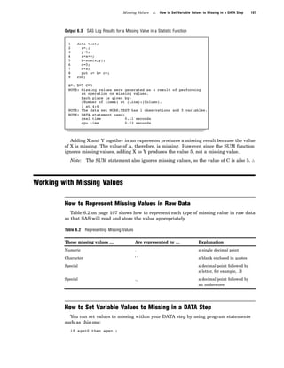
![SAS Language Elements 4 Pattern Matching Using SAS Regular Expressions (RX) and Perl Regular Expressions (PRX) 49
Metacharacter Description
B matches a non-word boundary:
3 "erB" matches the "er" in "verb"
3 "erB" does not match the "er" in "never"
d matches a digit character that is equivalent to [0-9].
D matches a non-digit character that is equivalent to [^0-9].
s matches any white space character including space, tab, form feed,
and so on, and is equivalent to [fnrtv].
S matches any character that is not a white space character and is
equivalent to [^fnrtv].
t matches a tab character and is equivalent to "x09".
w matches any word character including the underscore and is
equivalent to [A-Za-z0-9_].
W matches any non-word character and is equivalent to [^A-Za-z0-9_].
num matches num, where num is a positive integer. This is a reference
back to captured matches:
3 "(.)1" matches two consecutive identical characters.
Example 1: Validating Data
You can test for a pattern of characters within a string. For example, you can
examine a string to determine whether it contains a correctly formatted telephone
number. This type of test is called data validation.
The following example validates a list of phone numbers. To be valid, a phone
number must have one of the following forms: (XXX) XXX-XXXX or XXX-XXX-XXXX.
data _null_; u
if _N_ = 1 then
do;
paren = "([2-9]dd) ?[2-9]dd-dddd"; v
dash = "[2-9]dd-[2-9]dd-dddd"; w
regexp = "/(" || paren || ")|(" || dash || ")/"; x
retain re;
re = prxparse(regexp); y
if missing(re) then U
do;
putlog "ERROR: Invalid regexp " regexp; V
stop;
end;
end;
length first last home business $ 16;
input first last home business;
if ^prxmatch(re, home) then W
putlog "NOTE: Invalid home phone number for " first last home;](https://image.slidesharecdn.com/saslanguagereferenceconcepts-150330003208-conversion-gate01/85/Sas-language-reference-concepts-59-320.jpg)
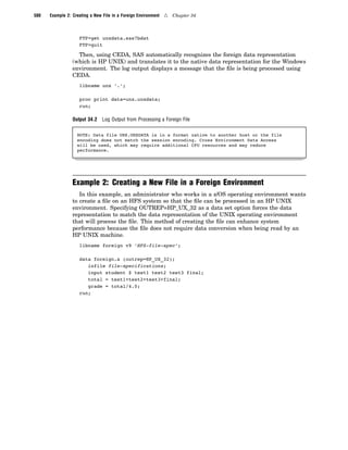
![50 Pattern Matching Using SAS Regular Expressions (RX) and Perl Regular Expressions (PRX) 4 Chapter 4
if ^prxmatch(re, business) then X
putlog "NOTE: Invalid business phone number for " first last business;
datalines;
Jerome Johnson (919)319-1677 (919)846-2198
Romeo Montague 800-899-2164 360-973-6201
Imani Rashid (508)852-2146 (508)366-9821
Palinor Kent . 919-782-3199
Ruby Archuleta . .
Takei Ito 7042982145 .
Tom Joad 209/963/2764 2099-66-8474
;
The following items correspond to the lines that are numbered in the DATA step that
is shown above.
u Create a DATA step.
v Build a Perl regular expression to identify a phone number that matches
(XXX)XXX-XXXX, and assign the variable PAREN to hold the result. Use the
following syntax elements to build the Perl regular expression:
( matches the open parenthesis in the area code.
[2–9] matches the digits 2–9. This is the first number in the area
code.
d matches a digit. This is the second number in the area code.
d matches a digit. This is the third number in the area code.
) matches the closed parenthesis in the area code.
? matches the space (which is the preceding subexpression) zero
or one time. Spaces are significant in Perl regular expressions.
They match a space in the text that you are searching. If a
space precedes the question mark metacharacter (as it does in
this case), the pattern matches either zero spaces or one space
in this position in the phone number.
w Build a Perl regular expression to identify a phone number that matches
XXX-XXX-XXXX, and assign the variable DASH to hold the result.
x Build a Perl regular expression that concatenates the regular expressions for
(XXX)XXX-XXXX and XXX—XXX—XXXX. The concatenation enables you to
search for both phone number formats from one regular expression.
The PAREN and DASH regular expressions are placed within parentheses. The
bar metacharacter (|) that is located between PAREN and DASH instructs the
compiler to match either pattern. The slashes around the entire pattern tell the
compiler where the start and end of the regular expression is located.
y Pass the Perl regular expression to PRXPARSE and compile the expression.
PRXPARSE returns a value to the compiled pattern. Using the value with other
Perl regular expression functions and CALL routines enables SAS to perform
operations with the compiled Perl regular expression.
U Use the MISSING function to check whether the regular expression was
successfully compiled.
V Use the PUTLOG statement to write an error message to the SAS log if the
regular expression did not compile.
W Search for a valid home phone number. PRXMATCH uses the value from
PRXPARSE along with the search text and returns the position where the regular](https://image.slidesharecdn.com/saslanguagereferenceconcepts-150330003208-conversion-gate01/85/Sas-language-reference-concepts-60-320.jpg)

![52 Pattern Matching Using SAS Regular Expressions (RX) and Perl Regular Expressions (PRX) 4 Chapter 4
w Use metacharacters to create a substitution syntax for a Perl regular expression,
and compile the expression. The substitution syntax specifies that a greater-than
character (>) in the input is replaced by the value > in the output.
x Use the MISSING function to check whether the Perl regular expression compiled
without error.
y Use the PUTLOG statement to write an error message to the SAS log if neither of
the regular expressions was found.
U Call the PRXCHANGE routine. Pass the LT_RE pattern-id, and search for and
replace all matching patterns. Put the results in _INFILE_ and write the
observation to the SAS log.
V Call the PRXCHANGE routine. Pass the GT_RE pattern-id, and search for and
replace all matching patterns. Put the results in _INFILE_ and write the
observation to the SAS log.
The following lines are written to the SAS log:
The bracketing construct ( ... ) creates capture buffers. To refer to
the digit’th buffer use <digit> within the match. Outside the match
use "$" instead of "". (The <digit> notation works in certain
circumstances outside the match. See the warning below about 1 vs $1
for details.) Referring back to another part of the match is called a
backreference.
Example 3: Extracting a Substring from a String
You can use Perl regular expressions to find and easily extract text from a string. In
this example, the DATA step creates a subset of North Carolina business phone
numbers. The program extracts the area code and checks it against a list of area codes
for North Carolina.
data _null_; u
if _N_ = 1 then
do;
paren = "(([2-9]dd)) ?[2-9]dd-dddd"; v
dash = "([2-9]dd)-[2-9]dd-dddd"; w
regexp = "/(" || paren || ")|(" || dash || ")/"; x
retain re;
re = prxparse(regexp); y
if missing(re) then U
do;
putlog "ERROR: Invalid regexp " regexp; V
stop;
end;
retain areacode_re;
areacode_re = prxparse("/828|336|704|910|919|252/"); W
if missing(areacode_re) then
do;
putlog "ERROR: Invalid area code regexp";
stop;
end;
end;
length first last home business $ 16;
length areacode $ 3;](https://image.slidesharecdn.com/saslanguagereferenceconcepts-150330003208-conversion-gate01/85/Sas-language-reference-concepts-62-320.jpg)
![SAS Language Elements 4 Pattern Matching Using SAS Regular Expressions (RX) and Perl Regular Expressions (PRX) 53
input first last home business;
if ^prxmatch(re, home) then
putlog "NOTE: Invalid home phone number for " first last home;
if prxmatch(re, business) then X
do;
which_format = prxparen(re); at
call prxposn(re, which_format, pos, len); ak
areacode = substr(business, pos, len);
if prxmatch(areacode_re, areacode) then al
put "In North Carolina: " first last business;
end;
else
putlog "NOTE: Invalid business phone number for " first last business;
datalines;
Jerome Johnson (919)319-1677 (919)846-2198
Romeo Montague 800-899-2164 360-973-6201
Imani Rashid (508)852-2146 (508)366-9821
Palinor Kent 704-782-4673 704-782-3199
Ruby Archuleta 905-384-2839 905-328-3892
Takei Ito 704-298-2145 704-298-4738
Tom Joad 515-372-4829 515-389-2838
;
The following items correspond to the numbered lines in the DATA step that is
shown above.
u Create a DATA step.
v Build a Perl regular expression to identify a phone number that matches
(XXX)XXX-XXXX, and assign the variable PAREN to hold the result. Use the
following syntax elements to build the Perl regular expression:
( matches the open parenthesis in the area code. The open
parenthesis marks the start of the submatch.
[2–9] matches the digits 2–9. This is the first number in the area
code.
d matches a digit. This is the second number in the area code.
d matches a digit. This is the third number in the area code.
) matches the closed parenthesis in the area code. The closed
parenthesis marks the end of the submatch.
? matches the space (which is the preceding subexpression) zero
or one time. Spaces are significant in Perl regular expressions.
They match a space in the text that you are searching. If a
space precedes the question mark metacharacter (as it does in
this case), the pattern matches either zero spaces or one space
in this position in the phone number.
w Build a Perl regular expression to identify a phone number that matches
XXX-XXX-XXXX, and assign the variable DASH to hold the result.
x Build a Perl regular expression that concatenates the regular expressions for
(XXX)XXX-XXXX and XXX—XXX—XXXX. The concatenation enables you to
search for both phone number formats from one regular expression.
The PAREN and DASH regular expressions are placed within parentheses. The
bar metacharacter (|) that is located between PAREN and DASH instructs the](https://image.slidesharecdn.com/saslanguagereferenceconcepts-150330003208-conversion-gate01/85/Sas-language-reference-concepts-63-320.jpg)
![54 Pattern Matching Using SAS Regular Expressions (RX) and Perl Regular Expressions (PRX) 4 Chapter 4
compiler to match either pattern. The slashes around the entire pattern tell the
compiler where the start and end of the regular expression is located.
y Pass the Perl regular expression to PRXPARSE and compile the expression.
PRXPARSE returns a value to the compiled pattern. Using the value with other
Perl regular expression functions and CALL routines enables SAS to perform
operations with the compiled Perl regular expression.
U Use the MISSING function to check whether the Perl regular expression compiled
without error.
V Use the PUTLOG statement to write an error message to the SAS log if the
regular expression did not compile.
W Compile a Perl regular expression that searches a string for a valid North
Carolina area code.
X Search for a valid business phone number.
at Use the PRXPAREN function to determine which submatch to use. PRXPAREN
returns the last submatch that was matched. If an area code matches the form
(XXX), PRXPAREN returns the value 2. If an area code matches the form XXX,
PRXPAREN returns the value 4.
ak Call the PRXPOSN routine to retrieve the position and length of the submatch.
al Use the PRXMATCH function to determine whether the area code is a valid North
Carolina area code, and write the observation to the log.
The following lines are written to the SAS log:
In North Carolina: Jerome Johnson (919)846-2198
In North Carolina: Palinor Kent 704-782-3199
In North Carolina: Takei Ito 704-298-4738
Writing Perl Debug Output to the SAS Log
The DATA step provides debugging support with the CALL PRXDEBUG routine.
CALL PRXDEBUG enables you to turn on and off Perl debug output messages that are
sent to the SAS log.
The following example writes Perl debug output to the SAS log.
data _null_;
/* CALL PRXDEBUG(1) turns on Perl debug output. */
call prxdebug(1);
putlog ’PRXPARSE: ’;
re = prxparse(’/[bc]d(ef*g)+h[ij]k$/’);
putlog ’PRXMATCH: ’;
pos = prxmatch(re, ’abcdefg_gh_’);
/* CALL PRXDEBUG(0) turns off Perl debug output. */
call prxdebug(0);
run;
SAS writes the following output to the log.](https://image.slidesharecdn.com/saslanguagereferenceconcepts-150330003208-conversion-gate01/85/Sas-language-reference-concepts-64-320.jpg)
![SAS Language Elements 4 Definition of ARM Macros 55
Output 4.3 SAS Debugging Output
PRXPARSE:
Compiling REx ‘[bc]d(ef*g)+h[ij]k$’
size 41 first at 1
rarest char g at 0
rarest char d at 0
1: ANYOF[bc](10)
10: EXACT <d>(12)
12: CURLYX[0] {1,32767}(26)
14: OPEN1(16)
16: EXACT <e>(18)
18: STAR(21)
19: EXACT <f>(0)
21: EXACT <g>(23)
23: CLOSE1(25)
25: WHILEM[1/1](0)
26: NOTHING(27)
27: EXACT <h>(29)
29: ANYOF[ij](38)
38: EXACT <k>(40)
40: EOL(41)
41: END(0)
anchored ‘de’ at 1 floating ‘gh’ at 3..2147483647 (checking floating) stclass
‘ANYOF[bc]’ minlen 7
PRXMATCH:
Guessing start of match, REx ‘[bc]d(ef*g)+h[ij]k$’ against ‘abcdefg_gh_’...
Did not find floating substr ‘gh’...
Match rejected by optimizer
For a detailed explanation of Perl debug output, see the “CALL PRXDEBUG
Routine” in SAS Language Reference: Dictionary.
Base SAS Functions for Web Applications
Four functions that manipulate Web-related content are available in Base SAS
software. HTMLENCODE and URLENCODE return encoded strings. HTMLDECODE
and URLDECODE return decoded strings. For information about Web-based SAS tools,
follow the Communities link on the SAS customer support home page, at
support.sas.com.
ARM Macros
Definition of ARM Macros
The ARM macros provide a way to measure the performance of applications as they
are executing. The macros write transaction records to the ARM log. The ARM log is an
external output text file that contains the logged ARM transaction records. You insert
the ARM macros into your SAS program at strategic points in order to generate calls to
the ARM API function calls. The ARM API function calls typically log the time of the
call and other related data to the log file. Measuring the time between these ARM API
function calls yields an approximate response-time measurement.
An ARM macro is self-contained and does not affect any code surrounding it,
provided that the variable name passed as an option to the ARM macro is unique. The](https://image.slidesharecdn.com/saslanguagereferenceconcepts-150330003208-conversion-gate01/85/Sas-language-reference-concepts-65-320.jpg)


![The SAS Registry 4 Definitions for the SAS Registry 235
3 The SASUSER library registry file contains the user defaults. When you change
your configuration information through a specialized window such as the Print
Setup window or the Explorer Options window, the settings are stored in the
SASUSER library.
How to Restore the Site Defaults
If you want to restore the original site defaults to your SAS session, delete the
regstry.sas7bitm file from your SASUSER library and restart your SAS session.
How Do I Display the SAS Registry?
You can use one of the following three methods to view the SAS registry:
3 Issue the REGEDIT command. This opens the SAS Registry Editor
3 Select Solutions I Accessories I Registry Editor
3 Submit the following line of code:
proc registry list;
run;
This method prints the registry to the SAS log, and it produces a large list that
contains all registry entries, including subkeys. Because of the large size, it might
take a few minutes to display the registry using this method.
For more information about how to view the SAS registry, see “The REGISTRY
Procedure” in Base SAS Procedures Guide.
Definitions for the SAS Registry
The SAS registry uses keys and subkeys as the basis for its structure, instead of using
directories and subdirectories like the file systems in DOS or UNIX. These terms and
several others described here are frequently used when discussing the SAS Registry:
key An entry in the registry file that refers to a particular aspect of SAS.
Each entry in the registry file consists of a key name, followed on
the next line by one or more values. Key names are entered on a
single line between square brackets ([ and ]).
The key can be a place holder without values or subkeys
associated with it, or it can have many subkeys with associated
values. Subkeys are delimited with a backslash (). The length of a
single key name or a sequence of key names cannot exceed 255
characters (including the square brackets and the backslash). Key
names can contain any character except the backslash and are not
case-sensitive.
The SAS Registry contains only one top-level key, called
SAS_REGISTRY. All the keys under SAS_REGISTRY are subkeys.](https://image.slidesharecdn.com/saslanguagereferenceconcepts-150330003208-conversion-gate01/85/Sas-language-reference-concepts-245-320.jpg)
![236 Managing the SAS Registry 4 Chapter 16
subkey A key inside another key. Subkeys are delimited with a backslash
(). Subkey names are not case-sensitive. The following key
contains one root key and two subkeys:
[SAS_REGISTRYHKEY_USER_ROOTCORE]
SAS_REGISTRY
is the root key.
HKEY_USER_ROOT
is a subkey of SAS_REGISTRY. In the SAS registry, there is
one other subkey at this level it is HKEY_SYSTEM_ROOT.
CORE
is a subkey of HKEY_USER_ROOT, containing many default
attributes for printers, windowing and so on.
link a value whose contents reference a key. Links are designed for
internal SAS use only. These values always begin with the word
“link:”.
value the names and content associated with a key or subkey. There are
two components to a value, the value name and the value content,
also known as a value datum.
Display 16.1 Section of the Registry Editor Showing Value Names and Value Data for
the Subkey ’HTML’
.SASXREG file a text file with the file extension .SASXREG that contains the text
representation of the actual binary SAS Registry file.
Managing the SAS Registry
Primary Concerns about Managing the SAS Registry
CAUTION:
If you make a mistake when you edit the registry, your system might become unstable or
unusable. Whenever possible, use the administrative tools, such as the New Library
window, the PRTDEF procedure, Universal Print windows, and the Explorer Options
window, to make configuration changes, rather than editing the registry. This is to
insure values are stored properly in the registry when changing the configuration. 4
CAUTION:
If you use the Registry Editor to change values, you will not be warned if any entry is
incorrect. Incorrect entries can cause errors, and can even prevent you from starting
a SAS session. 4](https://image.slidesharecdn.com/saslanguagereferenceconcepts-150330003208-conversion-gate01/85/Sas-language-reference-concepts-246-320.jpg)


![266 Setting Page Properties 4 Chapter 17
Definition wizard and on the Advanced tab of the Printer Properties window can be
prepopulated or “seeded” with a list of commands used to invoke print previewer
applications that are available at your site. Users and administrators can manually
update the registry, or define and import a registry file that contains a list of previewer
commands. An example of a registry file is:
[COREPRINTINGPREVIEW COMMANDS]
1=/usr/local/gv %s
2=/usr/local/ghostview %s
Previewing Print Jobs
You can use the print preview feature if a print viewer is installed for the designated
printer. Print Preview is always available from the File menu in SAS. You can also
issue the DMPRTPREVIEW command.
Setting Page Properties
For your current SAS session, you can customize how your printed output appears in
the Page Setup window. Depending on which printer you have currently set, some of
the Page Setup options that are described in the following steps may be unavailable.
To customize your printed output:
1 Issue the DMPAGESETUP command. The Page Setup window appears.
2 Select a tab to open windows that control various aspects of your printed output.
Descriptions of the tabbed windows follow.
The Page Setup window consists of four tabs: General, Orientation, Margins, and
Paper.
3 The General tab enables you to change the options for Binding, Collate, Duplex,
and Color Printing.
Display 17.17 Page Setup Window Displaying General Tab
Binding
specifies the binding edge (Long Edge or Short Edge) to use with duplexed
output. This sets the BINDING option.](https://image.slidesharecdn.com/saslanguagereferenceconcepts-150330003208-conversion-gate01/85/Sas-language-reference-concepts-276-320.jpg)


![Printing with SAS 4 Defining New Printers and Previewers with PROC PRTDEF 273
device = dummy;
dest = ;
run;
proc prtdef data=gsview list replace;
run;
Exporting and Backing Up Printer Definitions
PROC PRTEXP enables you to backup your printer definitions as a SAS data set that
can be restored with PROC PRTDEF.
PROC PRTEXP has the following syntax:
PROC PRTEXP [USESASHELP] [OUT=dataset]
[SELECT | EXCLUDE] printer_1 printer_2 ... printer_n;
The following example shows how to back up four printer definitions (named PDF,
postscript, PCL5 and PCL5c) using PROC PRTEXP.
proc prtexp out=printers;
select PDF postscript PCL5 PCL5c;
run;
For more information, see the PRTEXP procedure in Base SAS Procedures Guide.
Sample Values for the Device Type, Destination and Host Options Fields
The following list provides examples of the printer values for device type, destination
and host options. Because these values can be dependent on each other, and the values
can vary by operating environment, several different examples are shown. You might
want to refer to this list when you are installing or modifying a printer or when you
change the destination of your output.
3 Device Type: Printer
3 z/OS
3 Device type: Printer
3 Destination: (leave blank)
3 Host options: sysout=class-value dest=printer-name
3 UNIX and Windows
3 Device type: Printer
3 Destination: printer name
3 Host options: (leave blank)
3 VMS
3 Device type: Printer
3 Destination: printer name
3 Host options: passall=yes queue=printer-name](https://image.slidesharecdn.com/saslanguagereferenceconcepts-150330003208-conversion-gate01/85/Sas-language-reference-concepts-283-320.jpg)


![Array Processing 4 Rules for Referencing Arrays 447
proc print data=changed;
title ’Number of Books Sold’;
run;
The following output shows the CHANGED data set.
Output 25.1 Using an Array Statement to Process Missing Data Values
Number of Books Sold 1
Obs Reference Usage Introduction
1 45 63 113
2 0 75 150
3 62 0 98
Defining the Number of Elements in an Array
When you define the number of elements in an array, you can either use an asterisk
enclosed by braces ({*}), brackets ([*]), or parentheses ((*)) to count the number of
elements or to specify the number of elements. You must list each array element if you
use the asterisk to designate the number of elements. In the following example, the
array C1TEMP references five variables with temperature measures.
array c1temp{*} c1t1 c1t2 c1t3 c1t4 c1t5;
If you specify the number of elements explicitly, you can omit the names of the
variables or array elements in the ARRAY statement. SAS then creates variable names
by concatenating the array name with the numbers 1, 2, 3, and so on. If a variable
name in the series already exists, SAS uses that variable instead of creating a new one.
In the following example, the array c1t references five variables: c1t1, c1t2, c1t3, c1t4,
and c1t5.
array c1t{5};
Rules for Referencing Arrays
Before you make any references to an array, an ARRAY statement must appear in
the same DATA step that you used to create the array. Once you have created the
array, you can
3 use an array reference anywhere that you can write a SAS expression
3 use an array reference as the arguments of some SAS functions
3 use a subscript enclosed in braces, brackets, or parentheses to reference an array
3 use the special array subscript asterisk (*) to refer to all variables in an array in
an INPUT or PUT statement or in the argument of a function.
Note: You cannot use the asterisk with _TEMPORARY_ arrays. 4
An array definition is in effect only for the duration of the DATA step. If you want to
use the same array in several DATA steps, you must redefine the array in each step.
You can, however, redefine the array with the same variables in a later DATA step by](https://image.slidesharecdn.com/saslanguagereferenceconcepts-150330003208-conversion-gate01/85/Sas-language-reference-concepts-457-320.jpg)


Sas language reference concepts
- 2. The correct bibliographic citation for this manual is as follows: SAS Institute Inc. 2005. SAS ® 9.1.3 Language Reference: Concepts, Third Edition. Cary, NC: SAS Institute Inc. SAS® 9.1.3 Language Reference: Concepts, Third Edition Copyright © 2005, SAS Institute Inc., Cary, NC, USA ISBN 1-59047-905-X (e-book) ISBN-13: 978-1-59047-849-0 ISBN-10: 1-59047-840-1 (hard-copy book) All rights reserved. Produced in the United States of America. For a hard-copy book: No part of this publication may be reproduced, stored in a retrieval system, or transmitted, in any form or by any means, electronic, mechanical, photocopying, or otherwise, without the prior written permission of the publisher, SAS Institute Inc. For a Web download or e-book: Your use of this publication shall be governed by the terms established by the vendor at the time you acquire this publication. U.S. Government Restricted Rights Notice. Use, duplication, or disclosure of this software and related documentation by the U.S. government is subject to the Agreement with SAS Institute and the restrictions set forth in FAR 52.227-19 Commercial Computer Software-Restricted Rights (June 1987). SAS Institute Inc., SAS Campus Drive, Cary, North Carolina 27513. 1st printing, November 2005 SAS Publishing provides a complete selection of books and electronic products to help customers use SAS software to its fullest potential. For more information about our e-books, e-learning products, CDs, and hard-copy books, visit the SAS Publishing Web site at support.sas.com/pubs or call 1-800-727-3228. SAS® and all other SAS Institute Inc. product or service names are registered trademarks or trademarks of SAS Institute Inc. in the USA and other countries. ® indicates USA registration. Other brand and product names are registered trademarks or trademarks of their respective companies.
- 3. Contents P A R T 1 SAS System Concepts 1 Chapter 1 4 Essential Concepts of Base SAS Software 3 What Is SAS? 3 Overview of Base SAS Software 4 Components of the SAS Language 4 Ways to Run Your SAS Session 7 Customizing Your SAS Session 9 Conceptual Information about Base SAS Software 10 Chapter 2 4 SAS Processing 11 Definition of SAS Processing 11 Types of Input to a SAS Program 12 The DATA Step 13 The PROC Step 14 Chapter 3 4 Rules for Words and Names in the SAS Language 15 Words in the SAS Language 15 Names in the SAS Language 18 Chapter 4 4 SAS Language Elements 23 What Are the SAS Language Elements? 25 Data Set Options 25 Formats and Informats 27 Functions and CALL Routines 38 ARM Macros 55 Statements 69 SAS System Options 71 Chapter 5 4 SAS Variables 77 Definition of SAS Variables 78 SAS Variable Attributes 78 Ways to Create Variables 80 Variable Type Conversions 84 Aligning Variable Values 85 Automatic Variables 85 SAS Variable Lists 86 Dropping, Keeping, and Renaming Variables 88 Numeric Precision in SAS Software 90 Chapter 6 4 Missing Values 101 Definition of Missing Values 101
- 4. iv Special Missing Values 102 Order of Missing Values 103 When Variable Values Are Automatically Set to Missing by SAS 104 When Missing Values Are Generated by SAS 105 Working with Missing Values 107 Chapter 7 4 Expressions 109 Definitions for SAS Expressions 110 Examples of SAS Expressions 110 SAS Constants in Expressions 110 SAS Variables in Expressions 116 SAS Functions in Expressions 117 SAS Operators in Expressions 117 Chapter 8 4 Dates, Times, and Intervals 127 About SAS Date, Time, and Datetime Values 127 About Date and Time Intervals 137 Chapter 9 4 Error Processing and Debugging 147 Types of Errors in SAS 147 Error Processing in SAS 156 Debugging Logic Errors in the DATA Step 159 Chapter 10 4 SAS Output 161 Definitions for SAS Output 162 Routing SAS Output 163 The SAS Log 163 Traditional SAS Listing Output 167 Changing the Destination of the Log and the Output 170 Output Delivery System 170 Chapter 11 4 BY-Group Processing in SAS Programs 193 Definition of BY-Group Processing 193 References for BY-Group Processing 193 Chapter 12 4 WHERE-Expression Processing 195 Definition of WHERE-Expression Processing 195 Where to Use a WHERE Expression 196 Syntax of WHERE Expression 197 Combining Expressions by Using Logical Operators 205 Constructing Efficient WHERE Expressions 206 Processing a Segment of Data That Is Conditionally Selected 206 Deciding Whether to Use a WHERE Expression or a Subsetting IF Statement 208 Chapter 13 4 Optimizing System Performance 211 Definitions for Optimizing System Performance 211 Collecting and Interpreting Performance Statistics 212
- 5. v Techniques for Optimizing I/O 213 Techniques for Optimizing Memory Usage 218 Techniques for Optimizing CPU Performance 218 Calculating Data Set Size 219 Chapter 14 4 Support for Parallel Processing 221 Definition of Parallel Processing 221 Threaded I/O 221 Threaded Application Processing 222 Chapter 15 4 Monitoring Performance Using Application Response Measurement (ARM) 223 Introduction to ARM 223 How Does ARM Work? 225 Will ARM Affect an Application’s Performance? 225 Using the ARM Interface 226 Examples of Gathering Performance Data 229 Chapter 16 4 The SAS Registry 233 Introduction to the SAS Registry 234 Managing the SAS Registry 236 Configuring Your Registry 244 Chapter 17 4 Printing with SAS 247 Introduction to Universal Printing 248 Managing Printing Tasks with the Universal Printing User Interface 250 Configuring Universal Printing with Programming Statements 269 Forms Printing 275 P A R T 2 Windowing Environment Concepts 277 Chapter 18 4 Introduction to the SAS Windowing Environment 279 Basic Features of the SAS Windowing Environment 279 Main Windows of the SAS Windowing Environment 284 Chapter 19 4 Managing Your Data in the SAS Windowing Environment 301 Introduction to Managing Your Data in the SAS Windowing Environment 301 Copying and Viewing Files in a Data Library 301 Using the Workspace to Manipulate Data in a Data Set 306 Importing and Exporting Data 314 P A R T 3 DATA Step Concepts 319 Chapter 20 4 DATA Step Processing 321 Why Use a DATA Step? 322 Overview of DATA Step Processing 322 Processing a DATA Step: A Walkthrough 325
- 6. vi About DATA Step Execution 330 About Creating a SAS Data Set with a DATA Step 335 Writing a Report with a DATA Step 339 The DATA Step and ODS 347 Chapter 21 4 Reading Raw Data 349 Definition of Reading Raw Data 349 Ways to Read Raw Data 350 Kinds of Data 351 Sources of Raw Data 354 Reading Raw Data with the INPUT Statement 355 How SAS Handles Invalid Data 360 Reading Missing Values in Raw Data 360 Reading Binary Data 362 Reading Column-Binary Data 364 Chapter 22 4 BY-Group Processing in the DATA Step 367 Definitions for BY-Group Processing 367 Syntax for BY-Group Processing 368 Understanding BY Groups 369 Invoking BY-Group Processing 370 Determining Whether the Data Requires Preprocessing for BY-Group Processing 370 Preprocessing Input Data for BY-Group Processing 371 How the DATA Step Identifies BY Groups 372 Processing BY-Groups in the DATA Step 374 Chapter 23 4 Reading, Combining, and Modifying SAS Data Sets 379 Definitions for Reading, Combining, and Modifying SAS Data Sets 381 Overview of Tools 381 Reading SAS Data Sets 382 Combining SAS Data Sets: Basic Concepts 383 Combining SAS Data Sets: Methods 394 Error Checking When Using Indexes to Randomly Access or Update Data 420 Chapter 24 4 Using DATA Step Component Objects 429 Introduction 429 Using the Hash Object 430 Using the Hash Iterator Object 437 Chapter 25 4 Array Processing 441 Definitions for Array Processing 441 A Conceptual View of Arrays 442 Syntax for Defining and Referencing an Array 444 Processing Simple Arrays 444 Variations on Basic Array Processing 448 Multidimensional Arrays: Creating and Processing 449 Specifying Array Bounds 451
- 7. vii Examples of Array Processing 453 P A R T 4 SAS Files Concepts 459 Chapter 26 4 SAS Data Libraries 461 Definition of a SAS Data Library 461 Library Engines 463 Library Names 463 Accessing Remote SAS Libraries on SAS/CONNECT, SAS/SHARE, and WebDAV Servers 465 Library Concatenation 466 Permanent and Temporary Libraries 468 SAS System Libraries 469 Sequential Data Libraries 472 Tools for Managing Libraries 472 Chapter 27 4 SAS Data Sets 475 Definition of a SAS Data Set 475 Descriptor Information for a SAS Data Set 475 Data Set Names 476 Special SAS Data Sets 478 Sorted Data Sets 479 Tools for Managing Data Sets 479 Viewing and Editing SAS Data Sets 480 Chapter 28 4 SAS Data Files 481 Definition of a SAS Data File 483 Differences between Data Files and Data Views 483 Understanding an Audit Trail 485 Understanding Generation Data Sets 493 Understanding Integrity Constraints 499 Understanding SAS Indexes 512 Compressing Data Files 532 Chapter 29 4 SAS Data Views 535 Definition of SAS Data Views 535 Benefits of Using SAS Data Views 536 When to Use SAS Data Views 537 DATA Step Views 537 PROC SQL Views 541 Comparing DATA Step and PROC SQL Views 542 SAS/ACCESS Views 542 Chapter 30 4 Stored Compiled DATA Step Programs 545 Definition of a Stored Compiled DATA Step Program 545 Uses for Stored Compiled DATA Step Programs 545
- 8. viii Restrictions and Requirements for Stored Compiled DATA Step Programs 546 How SAS Processes Stored Compiled DATA Step Programs 546 Creating a Stored Compiled DATA Step Program 547 Executing a Stored Compiled DATA Step Program 549 Differences between Stored Compiled DATA Step Programs and DATA Step Views 552 Examples of DATA Step Programs 553 Chapter 31 4 DICTIONARY Tables 555 Definition of a DICTIONARY Table 555 How to View DICTIONARY Tables 555 Chapter 32 4 SAS Catalogs 559 Definition of a SAS Catalog 559 SAS Catalog Names 559 Tools for Managing SAS Catalogs 560 Profile Catalog 561 Catalog Concatenation 562 Chapter 33 4 About SAS/ACCESS Software 567 Definition of SAS/ACCESS Software 567 Dynamic LIBNAME Engine 567 SQL Procedure Pass-Through Facility 569 ACCESS Procedure and Interface View Engine 570 DBLOAD Procedure 571 Interface DATA Step Engine 571 Chapter 34 4 Processing Data Using Cross-Environment Data Access (CEDA) 573 Definition of Cross-Environment Data Access (CEDA) 573 Advantages of CEDA 574 SAS File Processing with CEDA 574 Processing a File with CEDA 576 Alternatives to Using CEDA 578 Creating New Files in a Foreign Data Representation 579 Examples of Using CEDA 579 Chapter 35 4 SAS 9.1 Compatibility with SAS Files From Earlier Releases 581 Introduction to Version Compatibility 581 Comparing SAS System 9 to Earlier Releases 581 Using SAS Library Engines 582 Chapter 36 4 File Protection 585 Definition of a Password 585 Assigning Passwords 586 Removing or Changing Passwords 588 Using Password-Protected SAS Files in DATA and PROC Steps 588 How SAS Handles Incorrect Passwords 589 Assigning Complete Protection with the PW= Data Set Option 589
- 9. ix Using Passwords with Views 590 SAS Data File Encryption 592 Chapter 37 4 SAS Engines 595 Definition of a SAS Engine 595 Specifying an Engine 595 How Engines Work with SAS Files 596 Engine Characteristics 597 About Library Engines 600 Special-Purpose Engines 602 Chapter 38 4 SAS File Management 605 Improving Performance of SAS Applications 605 Moving SAS Files Between Operating Environments 605 Repairing Damaged SAS Files 605 Chapter 39 4 External Files 609 Definition of External Files 609 Referencing External Files Directly 610 Referencing External Files Indirectly 610 Referencing Many External Files Efficiently 612 Referencing External Files with Other Access Methods 612 Working with External Files 613 P A R T 5 Industry Protocols Used in SAS 615 Chapter 40 4 The SMTP E-Mail Interface 617 Sending E-Mail through SMTP 617 System Options That Control SMTP E-Mail 617 Statements That Control SMTP E-mail 618 Chapter 41 4 Universal Unique Identifiers 619 Universal Unique Identifiers and the Object Spawner 619 Using SAS Language Elements to Assign UUIDs 621 P A R T 6 Appendices 623 Appendix 1 4 Recommended Reading 625 Recommended Reading 625 Index 627
- 10. x
- 11. 1 P A R T 1 SAS System Concepts Chapter 1. . . . . . . . . .Essential Concepts of Base SAS Software 3 Chapter 2. . . . . . . . . .SAS Processing 11 Chapter 3. . . . . . . . . .Rules for Words and Names in the SAS Language 15 Chapter 4. . . . . . . . . .SAS Language Elements 23 Chapter 5. . . . . . . . . .SAS Variables 77 Chapter 6. . . . . . . . . .Missing Values 101 Chapter 7. . . . . . . . . .Expressions 109 Chapter 8. . . . . . . . . .Dates, Times, and Intervals 127 Chapter 9. . . . . . . . . .Error Processing and Debugging 147 Chapter 10. . . . . . . . .SAS Output 161 Chapter 11. . . . . . . . .BY-Group Processing in SAS Programs 193 Chapter 12. . . . . . . . .WHERE-Expression Processing 195 Chapter 13. . . . . . . . .Optimizing System Performance 211 Chapter 14. . . . . . . . .Support for Parallel Processing 221 Chapter 15. . . . . . . . .Monitoring Performance Using Application Response Measurement (ARM) 223
- 12. 2 Chapter 16. . . . . . . . .The SAS Registry 233 Chapter 17. . . . . . . . .Printing with SAS 247
- 13. 3 C H A P T E R 1 Essential Concepts of Base SAS Software What Is SAS? 3 Overview of Base SAS Software 4 Components of the SAS Language 4 SAS Files 4 SAS Data Sets 5 External Files 5 Database Management System Files 6 SAS Language Elements 6 SAS Macro Facility 6 Ways to Run Your SAS Session 7 Starting a SAS Session 7 Different Types of SAS Sessions 7 SAS Windowing Environment 7 Interactive Line Mode 8 Noninteractive Mode 8 Batch Mode 9 Customizing Your SAS Session 9 Setting Default System Option Settings 9 Executing Statements Automatically 9 Customizing the SAS Windowing Environment 10 Conceptual Information about Base SAS Software 10 SAS System Concepts 10 DATA Step Concepts 10 SAS Files Concepts 10 What Is SAS? SAS is a set of solutions for enterprise-wide business users as well as a powerful fourth-generation programming language for performing tasks such as these: 3 data entry, retrieval, and management 3 report writing and graphics 3 statistical and mathematical analysis 3 business planning, forecasting, and decision support 3 operations research and project management 3 quality improvement 3 applications development With Base SAS software as the foundation, you can integrate with SAS many SAS business solutions that enable you to perform large scale business functions, such as
- 14. 4 Overview of Base SAS Software 4 Chapter 1 data warehousing and data mining, human resources management and decision support, financial management and decision support, and others. Overview of Base SAS Software The core of the SAS System is Base SAS software, which consists of the following: SAS language a programming language that you use to manage your data. SAS procedures software tools for data analysis and reporting. macro facility a tool for extending and customizing SAS software programs and for reducing text in your programs. DATA step debugger a programming tool that helps you find logic problems in DATA step programs. Output Delivery System (ODS) a system that delivers output in a variety of easy-to-access formats, such as SAS data sets, listing files, or Hypertext Markup Language (HTML). SAS windowing environment an interactive, graphical user interface that enables you to easily run and test your SAS programs. This document, along with SAS Language Reference: Dictionary, covers only the SAS language. For a complete guide to Base SAS software functionality, also see these documents: SAS Output Delivery System: User’s Guide, SAS National Language Support (NLS): User’s Guide, Base SAS Procedures Guide, SAS Metadata LIBNAME Engine: User’s Guide, SAS XML LIBNAME Engine User’s Guide, Base SAS Glossary, SAS Macro Language: Reference, and the Getting Started with SAS online tutorial. The SAS windowing environment is described in the online Help. Components of the SAS Language SAS Files When you work with SAS, you use files that are created and maintained by SAS, as well as files that are created and maintained by your operating environment, and that are not related to SAS. Files with formats or structures known to SAS are referred to as SAS files. All SAS files reside in a SAS data library. The most commonly used SAS file is a SAS data set. A SAS data set is structured in a format that SAS can process. Another common type of SAS file is a SAS catalog. Many different kinds of information that are used in a SAS job are stored in SAS catalogs, such as instructions for reading and printing data values, or function key settings that you use in the SAS windowing environment. A SAS stored program is a type of SAS file that contains compiled code that you create and save for repeated use. Operating Environment Information: In some operating environments, a SAS data library is a physical relationship among files; in others, it is a logical relationship. Refer to the SAS documentation for your operating environment for details about the characteristics of SAS data libraries in your operating environment. 4
- 15. Essential Concepts of Base SAS Software 4 External Files 5 SAS Data Sets There are two kinds of SAS data sets: 3 SAS data file 3 SAS data view. A SAS data file both describes and physically stores your data values. A SAS data view, on the other hand, does not actually store values. Instead, it is a query that creates a logical SAS data set that you can use as if it were a single SAS data set. It enables you to look at data stored in one or more SAS data sets or in other vendors’ software files. SAS data views enable you to create logical SAS data sets without using the storage space required by SAS data files. A SAS data set consists of the following: 3 descriptor information 3 data values. The descriptor information describes the contents of the SAS data set to SAS. The data values are data that has been collected or calculated. They are organized into rows, called observations, and columns, called variables. An observation is a collection of data values that usually relate to a single object. A variable is the set of data values that describe a given characteristic. The following figure represents a SAS data set. Figure 1.1 Representation of a SAS Data Set descriptor portion variables ID NAME TEAM STRTWGHT ENDWGHT data values observation 1023 1049 1219 1246 1078 David Shaw Amelia Serrano Alan Nance Ravi Sinha Ashley McKnight red yellow red yellow red 189 145 210 194 127 165 124 192 177 118 1 2 3 4 5 descriptive information Usually, an observation is the data that is associated with an entity such as an inventory item, a regional sales office, a client, or a patient in a medical clinic. Variables are characteristics of these entities, such as sale price, number in stock, and originating vendor. When data values are incomplete, SAS uses a missing value to represent a missing variable within an observation. External Files Data files that you use to read and write data, but which are in a structure unknown to SAS, are called external files. External files can be used for storing 3 raw data that you want to read into a SAS data file
- 16. 6 Database Management System Files 4 Chapter 1 3 SAS program statements 3 procedure output. Operating Environment Information: Refer to the SAS documentation for your operating environment for details about the characteristics of external files in your operating environment. 4 Database Management System Files SAS software is able to read and write data to and from other vendors’ software, such as many common database management system (DBMS) files. In addition to Base SAS software, you must license the SAS/ACCESS software for your DBMS and operating environment. SAS Language Elements The SAS language consists of statements, expressions, options, formats, and functions similar to those of many other programming languages. In SAS, you use these elements within one of two groups of SAS statements: 3 DATA steps 3 PROC steps. A DATA step consists of a group of statements in the SAS language that can 3 read data from external files 3 write data to external files 3 read SAS data sets and data views 3 create SAS data sets and data views. Once your data is accessible as a SAS data set, you can analyze the data and write reports by using a set of tools known as SAS procedures. A group of procedure statements is called a PROC step. SAS procedures analyze data in SAS data sets to produce statistics, tables, reports, charts, and plots, to create SQL queries, and to perform other analyses and operations on your data. They also provide ways to manage and print SAS files. You can also use global SAS statements and options outside of a DATA step or PROC step. SAS Macro Facility Base SAS software includes the SAS Macro Facility, a powerful programming tool for extending and customizing your SAS programs, and for reducing the amount of code that you must enter to do common tasks. Macros are SAS files that contain compiled macro program statements and stored text. You can use macros to automatically generate SAS statements and commands, write messages to the SAS log, accept input, or create and change the values of macro variables. For complete documentation, see SAS Macro Language: Reference.
- 17. Essential Concepts of Base SAS Software 4 SAS Windowing Environment 7 Ways to Run Your SAS Session Starting a SAS Session You start a SAS session with the SAS command, which follows the rules for other commands in your operating environment. In some operating environments, you include the SAS command in a file of system commands or control statements; in others, you enter the SAS command at a system prompt or select SAS from a menu. Different Types of SAS Sessions You can run SAS in any of several different ways that might be available for your operating environment: 3 SAS windowing environment 3 interactive line mode 3 noninteractive mode 3 batch (or background) mode. In addition, SAS/ASSIST software provides a menu-driven system for creating and running your SAS programs. For more information about SAS/ASSIST, see Getting Started with SAS/ASSIST. SAS Windowing Environment In the SAS windowing environment, you can edit and execute programming statements, display the SAS log, procedure output, and online Help, and more. The following figure shows the SAS windowing environment.
- 18. 8 Interactive Line Mode 4 Chapter 1 Figure 1.2 SAS Windowing Environment In the Explorer window, you can view and manage your SAS files, which are stored in libraries, and create shortcuts to external files. The Results window helps you navigate and manage output from SAS programs that you submit; you can view, save, and manage individual output items. You use the Program Editor, Log, and Output windows to enter, edit, and submit SAS programs, view messages about your SAS session and programs that you submit, and browse output from programs that you submit. For more detailed information about the SAS windowing environment, see Chapter 18, “Introduction to the SAS Windowing Environment,” on page 279. Interactive Line Mode In interactive line mode, you enter program statements in sequence in response to prompts from the SAS System. DATA and PROC steps execute when 3 a RUN, QUIT, or a semicolon on a line by itself after lines of data are entered 3 another DATA or PROC statement is entered 3 the ENDSAS statement is encountered. By default, the SAS log and output are displayed immediately following the program statements. Noninteractive Mode In noninteractive mode, SAS program statements are stored in an external file. The statements in the file execute immediately after you issue a SAS command referencing the file. Depending on your operating environment and the SAS system options that you use, the SAS log and output are either written to separate external files or displayed.
- 19. Essential Concepts of Base SAS Software 4 Executing Statements Automatically 9 Operating Environment Information: Refer to the SAS documentation for your operating environment for information about how these files are named and where they are stored. 4 Batch Mode You can run SAS jobs in batch mode in operating environments that support batch or background execution. Place your SAS statements in a file and submit them for execution along with the control statements and system commands required at your site. When you submit a SAS job in batch mode, one file is created to contain the SAS log for the job, and another is created to hold output that is produced in a PROC step or, when directed, output that is produced in a DATA step by a PUT statement. Operating Environment Information: Refer to the SAS documentation for your operating environment for information about executing SAS jobs in batch mode. Also, see the documentation specific to your site for local requirements for running jobs in batch and for viewing output from batch jobs. 4 Customizing Your SAS Session Setting Default System Option Settings You can use a configuration file to store system options with the settings that you want. When you invoke SAS, these settings are in effect. SAS system options determine how SAS initializes its interfaces with your computer hardware and the operating environment, how it reads and writes data, how output appears, and other global functions. By placing SAS system options in a configuration file, you can avoid having to specify the options every time that you invoke SAS. For example, you can specify the NODATE system option in your configuration file to prevent the date from appearing at the top of each page of your output. Operating Environment Information: See the SAS documentation for your operating environment for more information about the configuration file. In some operating environments, you can use both a system-wide and a user-specific configuration file. 4 Executing Statements Automatically To execute SAS statements automatically each time you invoke SAS, store them in an autoexec file. SAS executes the statements automatically after the system is initialized. You can activate this file by specifying the AUTOEXEC= system option. Any SAS statement can be included in an autoexec file. For example, you can set report titles, footnotes, or create macros or macro variables automatically with an autoexec file. Operating Environment Information: See the SAS documentation for your operating environment for information on how autoexec files should be set up so that they can be located by SAS. 4
- 20. 10 Customizing the SAS Windowing Environment 4 Chapter 1 Customizing the SAS Windowing Environment You can customize many aspects of the SAS windowing environment and store your settings for use in future sessions. With the SAS windowing environment, you can 3 change the appearance and sorting order of items in the Explorer window 3 customize the Explorer window by registering member, entry, and file types 3 set up favorite folders 3 customize the toolbar 3 set fonts, colors, and preferences. See the SAS online Help for more information and for additional ways to customize your SAS windowing environment. Conceptual Information about Base SAS Software SAS System Concepts SAS system-wide concepts include the building blocks of SAS language: rules for words and names, variables, missing values, expressions, dates, times, and intervals, and each of the six SAS language elements — data set options, formats, functions, informats, statements, and system options. SAS system-wide concepts also include introductory information that helps you begin to use SAS, including information about the SAS log, SAS output, error processing, WHERE processing, and debugging. Information about SAS processing prepares you to write SAS programs. Information on how to optimize system performance as well as how to monitor performance. DATA Step Concepts Understanding essential DATA step concepts can help you construct DATA step programs effectively. These concepts include how SAS processes the DATA step, how to read raw data to create a SAS data set, and how to write a report with a DATA step. More advanced concepts include how to combine and modify information once you have created a SAS data set, how to perform BY-group processing of your data, how to use array processing for more efficient programming, and how to create stored compiled DATA step programs. SAS Files Concepts SAS file concepts include advanced topics that are helpful for advanced applications, though not strictly necessary for writing simple SAS programs. These topics include the elements that comprise the physical file structure that SAS uses, including data libraries, data files, data views, catalogs, file protection, engines, and external files. Advanced topics for data files include the audit trail, generation data sets, integrity constraints, indexes, and file compression. In addition, these topics include compatibility issues with earlier releases and how to process files across operating environments.
- 21. 11 C H A P T E R 2 SAS Processing Definition of SAS Processing 11 Types of Input to a SAS Program 12 The DATA Step 13 DATA Step Output 13 The PROC Step 14 PROC Step Output 14 Definition of SAS Processing SAS processing is the way that the SAS language reads and transforms input data and generates the kind of output that you request. The DATA step and the procedure (PROC) step are the two steps in the SAS language. Generally, the DATA step manipulates data, and the PROC step analyzes data, produces output, or manages SAS files. These two types of steps, used alone or combined, form the basis of SAS programs. The following figure shows a high level view of SAS processing using a DATA step and a PROC step. The figure focuses primarily on the DATA step. Figure 2.1 SAS Processing Raw Data: External Files Instream Data Remote access through: Catalog FTP TCP/IP socket URL SAS Data Set SAS Data Sets: SAS Data Files SAS Data Views: PROC SQL Views (native) DATA Step Views (native) SAS/ACCESS Views (interface) DATA Step PROC Step External Files: SAS Log Reports External Data Files SAS Data Set Report SAS Log
- 22. 12 Types of Input to a SAS Program 4 Chapter 2 You can use different types of data as input to a DATA step. The DATA step is composed of SAS statements that you write, which contain instructions for processing the data. As each DATA step in a SAS program is compiling or executing, SAS generates a log that contains processing messages and error messages. These messages can help you debug a SAS program. Types of Input to a SAS Program You can use different sources of input data in your SAS program: SAS data sets can be one of two types: SAS data files store actual data values. A SAS data file consists of a descriptor portion that describes the data in the file, and a data portion. SAS data views contain references to data stored elsewhere. A SAS data view uses descriptor information and data from other files. It allow you to dynamically combine data from various sources, without using storage space to create a new data set. Data views consist of DATA step views, PROC SQL views, and SAS/ACCESS views. In most cases, you can use a SAS data view as if it were a SAS data file. For more information, see Chapter 28, “SAS Data Files,” on page 481, and Chapter 29, “SAS Data Views,” on page 535. Raw data specifies unprocessed data that have not been read into a SAS data set. You can read raw data from two sources: External files contain records comprised of formatted data (data are arranged in columns) or free-formatted data (data that are not arranged in columns). Instream data is data included in your program. You use the DATALINES statement at the beginning of your data to identify the instream data. For more information about raw data, see Chapter 21, “Reading Raw Data,” on page 349. Remote access allows you to read input data from nontraditional sources such as a TCP/IP socket or a URL. SAS treats this data as if it were coming from an external file. SAS allows you to access your input data remotely in the following ways: SAS catalog specifies the access method that enables you to reference a SAS catalog as an external file. FTP specifies the access method that enables you to use File Transfer Protocol (FTP) to read from or write to a file from any host machine that is connected to a network with an FTP server running. TCP/IP socket specifies the access method that enables you to read from or write to a Transmission Control Protocol/Internet Protocol (TCP/IP) socket.
- 23. SAS Processing 4 DATA Step Output 13 URL specifies the access method that enables you to use the Universal Resource Locator (URL) to read from and write to a file from any host machine that is connected to a network with a URL server running. For more information about accessing data remotely, see FILENAME, CATALOG Access Method; FILENAME, FTP Access Method; FILENAME, SOCKET Access Method; and FILENAME, URL Access Method statements in the Statements section of SAS Language Reference: Dictionary. The DATA Step The DATA step processes input data. In a DATA step, you can create a SAS data set, which can be a SAS data file or a SAS data view. The DATA step uses input from raw data, remote access, assignment statements, or SAS data sets. The DATA step can, for example, compute values, select specific input records for processing, and use conditional logic. The output from the DATA step can be of several types, such as a SAS data set or a report. You can also write data to the SAS log or to an external data file. For more information about DATA step processing, see Chapter 20, “DATA Step Processing,” on page 321. DATA Step Output The output from the DATA step can be a SAS data set or an external file such as the program log, a report, or an external data file. You can also update an existing file in place, without creating a separate data set. Data must be in the form of a SAS data set to be processed by many SAS procedures. You can create the following types of DATA step output: SAS log contains a list of processing messages and program errors. The SAS log is produced by default. SAS data file is a SAS data set that contains two parts: a data portion and a data descriptor portion. SAS data view is a SAS data set that uses descriptor information and data from other files. SAS data views allow you to dynamically combine data from various sources without using disk space to create a new data set. While a SAS data file actually contains data values, SAS data views contain only references to data stored elsewhere. SAS data views are of member type VIEW. In most cases, you can use a SAS data view as though it were a SAS data file. External data file contains the results of DATA step processing. These files are data or text files. The data can be records that are formatted or free-formatted. Report contains the results of DATA step processing. Although you usually generate a report by using a PROC step, you can generate the following two types of reports from the DATA step: Listing file contains printed results of DATA step processing, and usually contains headers and page breaks.
- 24. 14 The PROC Step 4 Chapter 2 HTML file contains results that you can display on the World Wide Web. This type of output is generated through the Output Delivery System (ODS). For complete information about ODS, see SAS Output Delivery System: User’s Guide. The PROC Step The PROC step consists of a group of SAS statements that call and execute a procedure, usually with a SAS data set as input. Use PROCs to analyze the data in a SAS data set, produce formatted reports or other results, or provide ways to manage SAS files. You can modify PROCs with minimal effort to generate the output you need. PROCs can also perform functions such as displaying information about a SAS data set. For more information about SAS procedures, see Base SAS Procedures Guide. PROC Step Output The output from a PROC step can provide univariate descriptive statistics, frequency tables, cross-tabulation tables, tabular reports consisting of descriptive statistics, charts, plots, and so on. Output can also be in the form of an updated data set. For more information about procedure output, see Base SAS Procedures Guide and SAS Output Delivery System: User’s Guide.
- 25. 15 C H A P T E R 3 Rules for Words and Names in the SAS Language Words in the SAS Language 15 Definition of Word 15 Types of Words or Tokens 16 Placement and Spacing of Words in SAS Statements 17 Spacing Requirements 17 Examples 17 Names in the SAS Language 18 Definition of a SAS Name 18 Rules for User-Supplied SAS Names 18 Rules for Most SAS Names 18 Rules for SAS Variable Names 20 SAS Name Literals 21 Definition of SAS Name Literals 21 Important Restrictions 21 Avoiding Errors When Using Name Literals 21 Examples 21 Words in the SAS Language Definition of Word A word or token in the SAS programming language is a collection of characters that communicates a meaning to SAS and which cannot be divided into smaller units that can be used independently. A word can contain a maximum of 32,767 characters. A word or token ends when SAS encounters one of the following: 3 the beginning of a new token 3 a blank after a name or a number token 3 the ending quotation mark of a literal token. Each word or token in the SAS language belongs to one of four categories: 3 names 3 literals 3 numbers 3 special characters.
- 26. 16 Types of Words or Tokens 4 Chapter 3 Types of Words or Tokens There are four basic types of words or tokens: name is a series of characters that begin with a letter or an underscore. Later characters can include letters, underscores, and numeric digits. A name token can contain up to 32,767 characters. In most contexts, however, SAS names are limited to a shorter maximum length, such as 32 or 8 characters. See Table 3.1 on page 19. Here are some examples of name tokens: 3 data 3 _new 3 yearcutoff 3 year_99 3 descending 3 _n_ literal consists of 1 to 32,767 characters enclosed in single or double quotation marks. Here are some examples of literals: 3 ’Chicago’ 3 "1990-91" 3 ’Amelia Earhart’ 3 ’Amelia Earhart’’s plane’ 3 "Report for the Third Quarter" Note: The surrounding quotation marks identify the token as a literal, but SAS does not store these marks as part of the literal token. 4 number in general, is composed entirely of numeric digits, with an optional decimal point and a leading plus or minus sign. SAS also recognizes numeric values in the following forms as number tokens: scientific (E−) notation, hexadecimal notation, missing value symbols, and date and time literals. Here are some examples of number tokens: 3 5683 3 2.35 3 0b0x 3 -5 3 5.4E-1 3 ’24aug90’d special character is usually any single keyboard character other than letters, numbers, the underscore, and the blank. In general, each special character is a single token, although some two-character operators, such as ** and <=, form single tokens. The blank can end a name or a number token, but it is not a token. Here are some
- 27. Rules for Words and Names in the SAS Language 4 Placement and Spacing of Words in SAS Statements 17 examples of special-character tokens: 3 = 3 ; 3 ’ 3 + 3 @ 3 / Placement and Spacing of Words in SAS Statements Spacing Requirements 1 You can begin SAS statements in any column of a line and write several statements on the same line. 2 You can begin a statement on one line and continue it on another line, but you cannot split a word between two lines. 3 A blank is not treated as a character in a SAS statement unless it is enclosed in quotation marks as a literal or part of a literal. Therefore, you can put multiple blanks any place in a SAS statement where you can put a single blank, with no effect on the syntax. 4 The rules for recognizing the boundaries of words or tokens determine the use of spacing between them in SAS programs. If SAS can determine the beginning of each token due to cues such as operators, you do not need to include blanks. If SAS cannot determine the beginning of each token, you must use blanks. See “Examples” on page 17. Although SAS does not have rigid spacing requirements, SAS programs are easier to read and maintain if you consistently indent statements. The examples illustrate useful spacing conventions. Examples 3 In this statement, blanks are not required because SAS can determine the boundary of every token by examining the beginning of the next token: total=x+y; The first special-character token, the equal sign, marks the end of the name token total. The plus sign, another special-character token, marks the end of the name token x. The last special-character token, the semicolon, marks the end of the y token. Though blanks are not needed to end any tokens in this example, you may add them for readability, as shown here: total = x + y; 3 This statement requires blanks because SAS cannot recognize the individual tokens without them: input group 15 room 20; Without blanks, the entire statement up to the semicolon fits the rules for a name token: it begins with a letter or underscore, contains letters, digits, or
- 28. 18 Names in the SAS Language 4 Chapter 3 underscores thereafter, and is less than 32,767 characters long. Therefore, this statement requires blanks to distinguish individual name and number tokens. Names in the SAS Language Definition of a SAS Name A SAS name is a name token that represents 3 variables 3 SAS data sets 3 formats or informats 3 SAS procedures 3 options 3 arrays 3 statement labels 3 SAS macros or macro variables 3 SAS catalog entries 3 librefs or filerefs. There are two kinds of names in SAS: 3 names of elements of the SAS language 3 names supplied by SAS users. Rules for User-Supplied SAS Names Rules for Most SAS Names Note: The rules are more flexible for SAS variable names than for other language elements. See “Rules for SAS Variable Names” on page 20. 4 1 The length of a SAS name depends on the element it is assigned to. Many SAS names can be 32 characters long; others have a maximum length of 8. 2 The first character must be a letter (A, B, C, . . ., Z) or underscore (_). Subsequent characters can be letters, numeric digits (0, 1, . . ., 9), or underscores. 3 You can use upper or lowercase letters. SAS processes names as uppercase regardless of how you type them. 4 Blanks cannot appear in SAS names. 5 Special characters, except for the underscore, are not allowed. In filerefs only, you can use the dollar sign ($), pound sign (#), and at sign (@). 6 SAS reserves a few names for automatic variables and variable lists, SAS data sets, and librefs. a When creating variables, do not use the names of special SAS automatic variables (for example, _N_ and _ERROR_) or special variable list names (for example, _CHARACTER_, _NUMERIC_, and _ALL_).
- 29. Rules for Words and Names in the SAS Language 4 Rules for User-Supplied SAS Names 19 b When associating a libref with a SAS data library, do not use these: SASHELP SASMSG SASUSER WORK c When you create SAS data sets, do not use these names: _NULL_ _DATA_ _LAST_ 7 When assigning a fileref to an external file, do not use: SASCAT 8 When you create a macro variable, do not use names that begin with SYS. Table 3.1 Maximum Length of User-Supplied SAS Names SAS Language Element Maximum Length Arrays 32 CALL routines 16 Catalog entries 32 DATA step statement labels 32 DATA step variable labels 256 DATA step variables 32 DATA step windows 32 Engines 8 Filerefs 8 Formats, character 31 Formats, numeric 32 Functions 16 Generation data sets 28 Informats, character 30 Informats, numeric 31 Librefs 8 Macro variables 32 Macro windows 32 Macros 32 Members of SAS data libraries (SAS data sets, views, catalogs, indexes) except for generation data sets 32 Passwords 8
- 30. 20 Rules for User-Supplied SAS Names 4 Chapter 3 SAS Language Element Maximum Length Procedure names (first 8 characters must be unique, and may not begin with “SAS”) 16 SCL variables 32 Rules for SAS Variable Names The rules for SAS variable names have expanded to provide more functionality. The setting of the VALIDVARNAME= system option determines what rules apply to the variables that you can create and process in your SAS session as well as to variables that you want to read from existing data sets. The VALIDVARNAME= option has three settings (V7, UPCASE, and ANY), each with varying degrees of flexibility for variable names: V7 is the default setting. Variable name rules are as follows: 1 SAS variable names can be up to 32 characters in length. 2 The first character must begin with an English letter or an underscore. Subsequent characters can be English letters, numeric digits, or underscores. 3 A variable name cannot contain blanks. 4 A variable name cannot contain any special characters other than the underscore. 5 A variable name can contain mixed case. Mixed case is remembered and used for presentation purposes only. (SAS stores the case used in the first reference to a variable.) When SAS processes variable names, however, it internally uppercases them. You cannot, therefore, use the same letters with different combinations of lowercase and uppercase to represent different variables. For example, cat, Cat, and CAT all represent the same variable. 6 You do not assign the names of special SAS automatic variables (such as _N_ and _ERROR_) or variable list names (such as _NUMERIC_, _CHARACTER_, and _ALL_) to variables. UPCASE is the same as V7, except that variable names are uppercased, as in earlier versions of SAS. ANY 1 SAS variable names can be up to 32 characters in length. 2 The name can start with or contain any characters, including blanks. CAUTION: Available for Base SAS procedures and SAS/STAT procedures only. VALIDVARNAME=ANY has been verified for use with only Base SAS procedures and SAS/STAT procedures. Any other use of this option is considered experimental and might cause undetected errors. 4 Note: If you use any characters other than English letters, numeric digits, or underscores, then you must express the variable name as a name literal and you must set VALIDVARNAME=ANY. If you use either the percent sign (%) or the ampersand (&), then you must use single quotation marks in the name literal in order to avoid interaction with the SAS Macro Facility. See “SAS Name Literals” on page 21. 4
- 31. Rules for Words and Names in the SAS Language 4 SAS Name Literals 21 3 A variable name can contain mixed case. Mixed case is stored and used for presentation purposes only. (SAS stores the case that is used in the first reference to a variable.) When SAS processes variable names, however, it internally uppercases them. Therefore, you cannot use the same letters with different combinations of lowercase and uppercase to represent different variables. For example, cat, Cat, and CAT all represent the same variable. SAS Name Literals Definition of SAS Name Literals A SAS name literal is a name token that is expressed as a string within quotation marks, followed by the letter n. Name literals allow you to use special characters (or blanks) that are not otherwise allowed in SAS names. Name literals are especially useful for expressing DBMS column and table names that contain special characters. Important Restrictions 3 You can use a name literal only for variables, statement labels, and DBMS column and table names. 3 You can use name literals in a DATA step or a PROC SQL step only. 3 When the name literal of a variable or DBMS column contains any characters that are not allowed when VALIDVARNAME=V7, then you must set the system option VALIDVARNAME=ANY. 3 If you use either the percent sign (%) or the ampersand (&), then you must use single quotation marks in the name literal in order to avoid interaction with the SAS Macro Facility. 3 When the name literal of a DBMS table or column contains any characters that are not valid for SAS rules, then you might need to specify a SAS/ACCESS LIBNAME statement option. 3 In a quoted string, SAS preserves and uses leading blanks, but SAS ignores and trims trailing blanks. Note: For more details and examples about the SAS/ACCESS LIBNAME statement and about using DBMS table and column names that do not conform to SAS naming conventions, see SAS/ACCESS for Relational Databases: Reference. 4 Avoiding Errors When Using Name Literals For information on how to avoid creating name literals in error, see “Avoiding a Common Error With Constants” on page 115. Examples Examples of SAS name literals are 3 input ’Bob’’s Asset Number’n; 3 input ’Bob"s Asset Number’n; 3 libname foo SAS/ACCESS-engine-name SAS/ACCESS-engine-connection-options;
- 32. 22 SAS Name Literals 4 Chapter 3 data foo.’My Table’n; 3 input ’Amount Budgeted’n ’Amount Spent’n ’Amount Difference’n;
- 33. 23 C H A P T E R 4 SAS Language Elements What Are the SAS Language Elements? 25 Data Set Options 25 Definition of Data Set Option 25 Syntax for Data Set Options 25 Using Data Set Options 25 Using Data Set Options with Input or Output SAS Data Sets 25 How Data Set Options Interact with System Options 26 Formats and Informats 27 Formats 27 Definition of a Format 27 Syntax of a Format 27 Ways to Specify Formats 28 Permanent versus Temporary Association 29 Informats 29 Definition of an Informat 29 Syntax of an Informat 29 Ways to Specify Informats 30 Permanent versus Temporary Association 31 User-Defined Formats and Informats 32 Byte Ordering for Integer Binary Data on Big Endian and Little Endian Platforms 32 Definitions 32 How Bytes Are Ordered 33 Writing Data Generated on Big Endian or Little Endian Platforms 33 Integer Binary Notation and Different Programming Languages 33 Working with Packed Decimal and Zoned Decimal Data 34 Definitions 34 Packed Decimal Data 34 Zoned Decimal Data 35 Packed Julian Dates 35 Platforms Supporting Packed Decimal and Zoned Decimal Data 35 Languages Supporting Packed Decimal and Zoned Decimal Data 35 Summary of Packed Decimal and Zoned Decimal Formats and Informats 36 Data Conversions and Encodings 38 Functions and CALL Routines 38 Definitions of Functions and CALL Routines 38 Definition of Functions 38 Definition of CALL Routines 39 Syntax of Functions and CALL Routines 39 Syntax of Functions 39 Syntax of CALL Routines 40 Using Functions 40
- 34. 24 Contents 4 Chapter 4 Restrictions on Function Arguments 40 Notes on Descriptive Statistic Functions 41 Notes on Financial Functions 41 Special Considerations for Depreciation Functions 41 Using DATA Step Functions within Macro Functions 42 Using Functions to Manipulate Files 42 Using Random-Number Functions and CALL Routines 43 Seed Values 43 Comparison of Random-Number Functions and CALL Routines 43 Example 1: Generating Multiple Streams from a CALL Routine 43 Example 2: Assigning Values from a Single Stream to Multiple Variables 44 Pattern Matching Using SAS Regular Expressions (RX) and Perl Regular Expressions (PRX) 45 Definition of Pattern Matching and Regular Expressions 45 Definition of SAS Regular Expression (RX) Functions and CALL Routines 45 Definition of Perl Regular Expression (PRX) Functions and CALL Routines 45 Benefits of Using Perl Regular Expressions in the DATA Step 46 Using Perl Regular Expressions in the DATA Step - License Agreement 46 Syntax of Perl Regular Expressions 47 Example 1: Validating Data 49 Example 2: Replacing Text 51 Example 3: Extracting a Substring from a String 52 Writing Perl Debug Output to the SAS Log 54 Base SAS Functions for Web Applications 55 ARM Macros 55 Definition of ARM Macros 55 Using ARM Macros 56 Overview of ARM Macros 56 Using Variables with ARM Macros 57 ARM API Objects 58 ID Management Using ARM Macros 58 Complex ARM Macro Call Schemes 61 Defining User Metrics in ARM Macros 63 Defining Correlators in ARM Macros 64 Enabling ARM Macro Execution 65 Setting the _ARMEXEC Macro Variable 65 Enabling ARM Macro Execution with SCL 66 Conditional ARM Macro Execution 66 Setting the Macro Environment 67 Using ARM Post-Processing Macros 68 Statements 69 Definition of Statements 69 Executable and Declarative DATA Step Statements 69 Global Statements 70 SAS System Options 71 Definition of SAS System Options 71 Syntax of SAS System Options 71 Using SAS System Options 71 Default Settings 71 Determining Which Settings Are in Effect 71 Determining Which SAS System Options Are Restricted 72 Determining How a SAS System Option Value Was Set 72 Obtaining Descriptive Information about a System Option 73 Changing SAS System Option Settings 73 How Long System Option Settings Are in Effect 74
- 35. SAS Language Elements 4 Using Data Set Options 25 Order of Precedence 75 Interaction with Data Set Options 75 Comparisons 76 What Are the SAS Language Elements? The major language elements of Base SAS software are as follows: 3 data set options 3 formats and informats 3 functions and CALL routines 3 Application Response Measurement (ARM) macros 3 statements 3 SAS system options For detailed information on each language element, see SAS Language Reference: Dictionary. Data Set Options Definition of Data Set Option Data set options specify actions that apply only to the SAS data set with which they appear. They enable you to perform operations such as these: 3 renaming variables 3 selecting only the first or last n observations for processing 3 dropping variables from processing or from the output data set 3 specifying a password for a data set. Syntax for Data Set Options Specify a data set option in parentheses after a SAS data set name. To specify several data set options, separate them with spaces. (option-1=value-1<...option-n=value-n>) These examples show data set options in SAS statements: data scores(keep=team game1 game2 game3); proc print data=new(drop=year); set old(rename=(date=Start_Date)); Using Data Set Options Using Data Set Options with Input or Output SAS Data Sets Most SAS data set options can apply to either input or output SAS data sets in DATA steps or procedure (PROC) steps. If a data set option is associated with an input data
- 36. 26 Using Data Set Options 4 Chapter 4 set, the action applies to the data set that is being read. If the option appears in the DATA statement or after an output data set specification in a PROC step, SAS applies the action to the output data set. In the DATA step, data set options for output data sets must appear in the DATA statement, not in any OUTPUT statements that might be present. Some data set options, such as COMPRESS=, are meaningful only when you create a SAS data set because they set attributes that exist for the life of the data set. To change or cancel most data set options, you must re-create the data set. You can change other options (such as PW= and LABEL=) with PROC DATASETS. For more information, see “The DATASETS Procedure” in Base SAS Procedures Guide. When data set options appear on both input and output data sets in the same DATA or PROC step, SAS applies data set options to input data sets before it evaluates programming statements or before it applies data set options to output data sets. Likewise, data set options that are specified for the data set being created are applied after programming statements are processed. For example, when using the RENAME= data set option, the new names are not associated with the variables until the DATA step ends. In some instances, data set options conflict when they are used in the same statement. For example, you cannot specify both the DROP= and KEEP= options for the same variable in the same statement. Timing can also be an issue in some cases. For example, if using KEEP= and RENAME= on a data set specified in the SET statement, KEEP= needs to use the original variable names, because SAS will process KEEP= before the data set is read. The new names specified in RENAME= will apply to the programming statements that follow the SET statement. How Data Set Options Interact with System Options Many system options and data set options share the same name and have the same function. System options remain in effect for all DATA and PROC steps in a SAS job or session, unless they are respecified. The data set option overrides the system option for the data set in the step in which it appears. In this example, the OBS= system option in the OPTIONS statement specifies that only the first 100 observations will be processed from any data set within the SAS job. The OBS= data set option in the SET statement, however, overrides the system option for data set TWO and specifies that only the first 5 observations will be read from data set TWO. The PROC PRINT step prints the data set FINAL. This data set contains the first 5 observations from data set TWO, followed by the first 100 observations from data set THREE: options obs=100; data final; set two(obs=5) three; run; proc print data=final; run;
- 37. SAS Language Elements 4 Formats 27 Formats and Informats Formats Definition of a Format A format is an instruction that SAS uses to write data values. You use formats to control the written appearance of data values, or, in some cases, to group data values together for analysis. For example, the WORDS22. format, which converts numeric values to their equivalent in words, writes the numeric value 692 as six hundred ninety-two. Syntax of a Format SAS formats have the following form: <$>format<w>.<d> Here is an explanation of the syntax: $ indicates a character format; its absence indicates a numeric format. format names the format. The format is a SAS format or a user-defined format that was previously defined with the VALUE statement in PROC FORMAT. For more information on user-defined formats, see “The FORMAT Procedure” in Base SAS Procedures Guide. w specifies the format width, which for most formats is the number of columns in the output data. d specifies an optional decimal scaling factor in the numeric formats. Formats always contain a period (.) as a part of the name. If you omit the w and the d values from the format, SAS uses default values. The d value that you specify with a format tells SAS to display that many decimal places, regardless of how many decimal places are in the data. Formats never change or truncate the internally stored data values. For example, in DOLLAR10.2, the w value of 10 specifies a maximum of 10 columns for the value. The d value of 2 specifies that two of these columns are for the decimal part of the value, which leaves eight columns for all the remaining characters in the value. This includes the decimal point, the remaining numeric value, a minus sign if the value is negative, the dollar sign, and commas, if any. If the format width is too narrow to represent a value, then SAS tries to squeeze the value into the space available. Character formats truncate values on the right. Numeric formats sometimes revert to the BESTw.d format. SAS prints asterisks if you do not specify an adequate width. In the following example, the result is x=**. x=123; put x=2.; If you use an incompatible format, such as using a numeric format to write character values, first SAS attempts to use an analogous format of the other type. If this is not feasible, then an error message that describes the problem appears in the SAS log.
- 38. 28 Formats 4 Chapter 4 Ways to Specify Formats You can use formats in the following ways: 3 in a PUT statement The PUT statement with a format after the variable name uses a format to write data values in a DATA step. For example, this PUT statement uses the DOLLAR. format to write the numeric value for AMOUNT as a dollar amount: amount=1145.32; put amount dollar10.2; The DOLLARw.d format in the PUT statement produces this result: $1,145.32 See the “PUT Statement” in SAS Language Reference: Dictionary for more information. 3 with the PUT, PUTC, or PUTN functions The PUT function writes a numeric variable, a character variable, or a constant with any valid format and returns the resulting character value. For example, the following statement converts the value of a numeric variable into a two-character hexadecimal representation: num=15; char=put(num,hex2.); The PUT function creates a character variable named CHAR that has a value of 0F. The PUT function is useful for converting a numeric value to a character value. See the “PUT Function” in SAS Language Reference: Dictionary for more information. 3 with the %SYSFUNC macro function The %SYSFUNC (or %QSYSFUNC) macro function executes SAS functions or user-defined functions and applies an optional format to the result of the function outside a DATA step. For example, the following program writes a numeric value in a macro variable as a dollar amount. %macro tst(amount); %put %sysfunc(putn(&amount,dollar10.2)); %mend tst; %tst (1154.23); For more information, see SAS Macro Language: Reference. 3 in a FORMAT statement in a DATA step or a PROC step. The FORMAT statement permanently associates a format with a variable. SAS uses the format to write the values of the variable that you specify. For example, the following statement in a DATA step associates the COMMAw.d numeric format with the variables SALES1 through SALES3: format sales1-sales3 comma10.2; Because the FORMAT statement permanently associates a format with a variable, any subsequent DATA step or PROC step uses COMMA10.2 to write the values of SALES1, SALES2, and SALES3. See the “FORMAT Statement” in SAS Language Reference: Dictionary for more information. Note: Formats that you specify in a PUT statement behave differently from those that you associate with a variable in a FORMAT statement. The major
- 39. SAS Language Elements 4 Informats 29 difference is that formats that are specified in the PUT statement will preserve leading blanks. If you assign formats with a FORMAT statement prior to a PUT statement, all leading blanks are trimmed. The result is the same as if you used the colon (:) format modifier. For details about using the colon (:) format modifier, see the “PUT Statement, List” in SAS Language Reference: Dictionary. 4 3 in an ATTRIB statement in a DATA step or a PROC step. The ATTRIB statement can also associate a format, as well as other attributes, with one or more variables. For example, in the following statement the ATTRIB statement permanently associates the COMMAw.d format with the variables SALES1 through SALES3: attrib sales1-sales3 format=comma10.2; Because the ATTRIB statement permanently associates a format with a variable, any subsequent DATA step or PROC step uses COMMA10.2 to write the values of SALES1, SALES2, and SALES3. For more information, see the “ATTRIB Statement” in SAS Language Reference: Dictionary. Permanent versus Temporary Association When you specify a format in a PUT statement, SAS uses the format to write data values during the DATA step but does not permanently associate the format with a variable. To permanently associate a format with a variable, use a FORMAT statement or an ATTRIB statement in a DATA step. SAS permanently associates a format with the variable by modifying the descriptor information in the SAS data set. Using a FORMAT statement or an ATTRIB statement in a PROC step associates a format with a variable for that PROC step, as well as for any output data sets that the procedure creates that contain formatted variables. For more information on using formats in SAS procedures, see Base SAS Procedures Guide. Informats Definition of an Informat An informat is an instruction that SAS uses to read data values into a variable. For example, the following value contains a dollar sign and commas: $1,000,000 To remove the dollar sign ($) and commas (,) before storing the numeric value 1000000 in a variable, read this value with the COMMA11. informat. Unless you explicitly define a variable first, SAS uses the informat to determine whether the variable is numeric or character. SAS also uses the informat to determine the length of character variables. Syntax of an Informat SAS informats have the following form: <$>informat<w>.<d> Here is an explanation of the syntax: $ indicates a character informat; its absence indicates a numeric informat.
- 40. 30 Informats 4 Chapter 4 informat names the informat. The informat is a SAS informat or a user-defined informat that was previously defined with the INVALUE statement in PROC FORMAT. For more information on user-defined informats, see “The FORMAT Procedure” in Base SAS Procedures Guide. w specifies the informat width, which for most informats is the number of columns in the input data. d specifies an optional decimal scaling factor in the numeric informats. SAS divides the input data by 10 to the power of d. Note: Even though SAS can read up to 31 decimal places when you specify some numeric informats, floating-point numbers with more than 12 decimal places might lose precision due to the limitations of the eight-byte floating point representation used by most computers. 4 Informats always contain a period (.) as a part of the name. If you omit the w and the d values from the informat, SAS uses default values. If the data contains decimal points, SAS ignores the d value and reads the number of decimal places that are actually in the input data. If the informat width is too narrow to read all the columns in the input data, you may get unexpected results. The problem frequently occurs with the date and time informats. You must adjust the width of the informat to include blanks or special characters between the day, month, year, or time. For more information about date and time values, see Chapter 8, “Dates, Times, and Intervals,” on page 127. When a problem occurs with an informat, SAS writes a note to the SAS log and assigns a missing value to the variable. Problems occur if you use an incompatible informat, such as a numeric informat to read character data, or if you specify the width of a date and time informat that causes SAS to read a special character in the last column. Ways to Specify Informats You can specify informats in the following ways: 3 in an INPUT statement The INPUT statement with an informat after a variable name is the simplest way to read values into a variable. For example, the following INPUT statement uses two informats: input @15 style $3. @21 price 5.2; The $w. character informat reads values into the variable STYLE. The w.d numeric informat reads values into the variable PRICE. For a complete discussion of the “INPUT Statement” , see SAS Language Reference: Dictionary. 3 with the INPUT, INPUTC, and INPUTN functions The INPUT function reads a SAS character expression using a specified informat. The informat determines whether the resulting value is numeric or character. Thus, the INPUT function is useful for converting data. For example, TempCharacter=’98.6’; TemperatureNumber=input(TempCharacter,4.); Here, the INPUT function in combination with the w.d informat reads the character value of TempCharacter as a numeric value and assigns the numeric value 98.6 to TemperatureNumber.
- 41. SAS Language Elements 4 Informats 31 Use the PUT function with a SAS format to convert numeric values to character values. See the “PUT Function” in SAS Language Reference: Dictionary for an example of a numeric-to-character conversion. For a complete discussion of the “INPUT Function”, see SAS Language Reference: Dictionary. 3 in an INFORMAT statement in a DATA or a PROC step The INFORMAT statement associates an informat with a variable. SAS uses the informat in any subsequent INPUT statement to read values into the variable. For example, in the following statements the INFORMAT statement associates the DATEw. informat with the variables Birthdate and Interview: informat Birthdate Interview date9.; input @63 Birthdate Interview; An informat that is associated with an INFORMAT statement behaves like an informat that you specify with a colon (:) format modifier in an INPUT statement. (For details about using the colon (:) modifier, see the “INPUT Statement, List” in SAS Language Reference: Dictionary.) Therefore, SAS uses a modified list input to read the variable so that 3 the w value in an informat does not determine column positions or input field widths in an external file 3 the blanks that are embedded in input data are treated as delimiters unless you change the DELIMITER= option in an INFILE statement 3 for character informats, the w value in an informat specifies the length of character variables 3 for numeric informats, the w value is ignored 3 for numeric informats, the d value in an informat behaves in the usual way for numeric informats If you have coded the INPUT statement to use another style of input, such as formatted input or column input, that style of input is not used when you use the INFORMAT statement. See the “INPUT Statement, List” in SAS Language Reference: Dictionary for more information about how to use modified list input to read data. 3 in an ATTRIB statement in a DATA or a PROC step. The ATTRIB statement can also associate an informat, as well as other attributes, with one or more variables. For example, in the following statements, the ATTRIB statement associates the DATEw. informat with the variables Birthdate and Interview: attrib Birthdate Interview informat=date9.; input @63 Birthdate Interview; An informat that is associated by using the INFORMAT= option in the ATTRIB statement behaves like an informat that you specify with a colon (:) format modifier in an INPUT statement. (For details about using the colon (:) modifier, see the “INPUT Statement, List” in SAS Language Reference: Dictionary.) Therefore, SAS uses a modified list input to read the variable in the same way as it does for the INFORMAT statement. See the “ATTRIB Statement” in SAS Language Reference: Dictionary for more information. Permanent versus Temporary Association When you specify an informat in an INPUT statement, SAS uses the informat to read input data values during that DATA step. SAS, however, does not permanently associate
- 42. 32 User-Defined Formats and Informats 4 Chapter 4 the informat with the variable. To permanently associate a format with a variable, use an INFORMAT statement or an ATTRIB statement. SAS permanently associates an informat with the variable by modifying the descriptor information in the SAS data set. User-Defined Formats and Informats In addition to the formats and informats that are supplied with Base SAS software, you can create your own formats and informats. In Base SAS software, PROC FORMAT allows you to create your own formats and informats for both character and numeric variables. When you execute a SAS program that uses user-defined formats or informats, these formats and informats should be available. The two ways to make these formats and informats available are 3 to create permanent, not temporary, formats or informats with PROC FORMAT 3 to store the source code that creates the formats or informats (the PROC FORMAT step) with the SAS program that uses them. To create permanent SAS formats and informats, see “The FORMAT Procedure” in Base SAS Procedures Guide. If you execute a program that cannot locate a user-defined format or informat, the result depends on the setting of the FMTERR system option. If the user-defined format or informat is not found, then these system options produce these results: System option Results FMTERR SAS produces an error that causes the current DATA or PROC step to stop. NOFMTERR SAS continues processing and substitutes a default format, usually the BESTw. or $w. format. Although using NOFMTERR enables SAS to process a variable, you lose the information that the user-defined format or informat supplies. To avoid problems, make sure that your program has access to all of the user-defined formats and informats that are used in the program. Byte Ordering for Integer Binary Data on Big Endian and Little Endian Platforms Definitions Integer values for binary integer data are typically stored in one of three sizes: one-byte, two-byte, or four-byte. The ordering of the bytes for the integer varies depending on the platform (operating environment) on which the integers were produced. The ordering of bytes differs between the “big endian” and “little endian” platforms. These colloquial terms are used to describe byte ordering for IBM mainframes (big endian) and for Intel-based platforms (little endian). In SAS, the following platforms are considered big endian: AIX, HP-UX, IBM mainframe, Macintosh, and Solaris. The following platforms are considered little endian: OpenVMS Alpha, Digital UNIX, Intel ABI, and Windows.
- 43. SAS Language Elements 4 Byte Ordering for Integer Binary Data on Big Endian and Little Endian Platforms 33 How Bytes Are Ordered On big endian platforms, the value 1 is stored in binary and is represented here in hexadecimal notation. One byte is stored as 01, two bytes as 00 01, and four bytes as 00 00 00 01. On little endian platforms, the value 1 is stored in one byte as 01 (the same as big endian), in two bytes as 01 00, and in four bytes as 01 00 00 00. If an integer is negative, the “two’s complement” representation is used. The high-order bit of the most significant byte of the integer will be set on. For example, –2 would be represented in one, two, and four bytes on big endian platforms as FE, FF FE, and FF FF FF FE respectively. On little endian platforms, the representation would be FE, FE FF, and FE FF FF FF. These representations result from the output of the integer binary value –2 expressed in hexadecimal representation. Writing Data Generated on Big Endian or Little Endian Platforms SAS can read signed and unsigned integers regardless of whether they were generated on a big endian or a little endian system. Likewise, SAS can write signed and unsigned integers in both big endian and little endian format. The length of these integers can be up to eight bytes. The following table shows which format to use for various combinations of platforms. In the Sign? column, “no” indicates that the number is unsigned and cannot be negative. “Yes” indicates that the number can be either negative or positive. Table 4.1 SAS Formats and Byte Ordering Data created for... Data written by... Sign? Format/Informat big endian big endian yes IB or S370FIB big endian big endian no PIB, S370FPIB, S370FIBU big endian little endian yes S370FIB big endian little endian no S370FPIB little endian big endian yes IBR little endian big endian no PIBR little endian little endian yes IB or IBR little endian little endian no PIB or PIBR big endian either yes S370FIB big endian either no S370FPIB little endian either yes IBR little endian either no PIBR Integer Binary Notation and Different Programming Languages The following table compares integer binary notation according to programming language.
- 44. 34 Working with Packed Decimal and Zoned Decimal Data 4 Chapter 4 Table 4.2 Integer Binary Notation and Programming Languages Language 2 Bytes 4 Bytes SAS IB2., IBR2., PIB2., PIBR2., S370FIB2., S370FIBU2., S370FPIB2. IB4., IBR4., PIB4., PIBR4., S370FIB4., S370FIBU4., S370FPIB4. PL/I FIXED BIN(15) FIXED BIN(31) FORTRAN INTEGER*2 INTEGER*4 COBOL COMP PIC 9(4) COMP PIC 9(8) IBM assembler H F C short long Working with Packed Decimal and Zoned Decimal Data Definitions Packed decimal specifies a method of encoding decimal numbers by using each byte to represent two decimal digits. Packed decimal representation stores decimal data with exact precision. The fractional part of the number is determined by the informat or format because there is no separate mantissa and exponent. An advantage of using packed decimal data is that exact precision can be maintained. However, computations involving decimal data might become inexact due to the lack of native instructions. Zoned decimal specifies a method of encoding decimal numbers in which each digit requires one byte of storage. The last byte contains the number’s sign as well as the last digit. Zoned decimal data produces a printable representation. Nibble specifies 1/2 of a byte. Packed Decimal Data A packed decimal representation stores decimal digits in each “nibble” of a byte. Each byte has two nibbles, and each nibble is indicated by a hexadecimal digit. For example, the value 15 is stored in two nibbles, using the hexadecimal digits 1 and 5. The sign indication is dependent on your operating environment. On IBM mainframes, the sign is indicated by the last nibble. With formats, C indicates a positive value, and D indicates a negative value. With informats, A, C, E, and F indicate positive values, and B and D indicate negative values. Any other nibble is invalid for signed packed decimal data. In all other operating environments, the sign is indicated in its own byte. If the high-order bit is 1, then the number is negative. Otherwise, it is positive. The following applies to packed decimal data representation: 3 You can use the S370FPD format on all platforms to obtain the IBM mainframe configuration.
- 45. SAS Language Elements 4 Working with Packed Decimal and Zoned Decimal Data 35 3 You can have unsigned packed data with no sign indicator. The packed decimal format and informat handles the representation. It is consistent between ASCII and EBCDIC platforms. 3 Note that the S370FPDU format and informat expects to have an F in the last nibble, while packed decimal expects no sign nibble. Zoned Decimal Data The following applies to zoned decimal data representation: 3 A zoned decimal representation stores a decimal digit in the low order nibble of each byte. For all but the byte containing the sign, the high-order nibble is the numeric zone nibble (F on EBCDIC and 3 on ASCII). 3 The sign can be merged into a byte with a digit, or it can be separate, depending on the representation. But the standard zoned decimal format and informat expects the sign to be merged into the last byte. 3 The EBCDIC and ASCII zoned decimal formats produce the same printable representation of numbers. There are two nibbles per byte, each indicated by a hexadecimal digit. For example, the value 15 is stored in two bytes. The first byte contains the hexadecimal value F1 and the second byte contains the hexadecimal value C5. Packed Julian Dates The following applies to packed Julian dates: 3 The two formats and informats that handle Julian dates in packed decimal representation are PDJULI and PDJULG. PDJULI uses the IBM mainframe year computation, while PDJULG uses the Gregorian computation. 3 The IBM mainframe computation considers 1900 to be the base year, and the year values in the data indicate the offset from 1900. For example, 98 means 1998, 100 means 2000, and 102 means 2002. 1998 would mean 3898. 3 The Gregorian computation allows for 2-digit or 4-digit years. If you use 2-digit years, SAS uses the setting of the YEARCUTOFF= system option to determine the true year. Platforms Supporting Packed Decimal and Zoned Decimal Data Some platforms have native instructions to support packed and zoned decimal data, while others must use software to emulate the computations. For example, the IBM mainframe has an Add Pack instruction to add packed decimal data, but the Intel-based platforms have no such instruction and must convert the decimal data into some other format. Languages Supporting Packed Decimal and Zoned Decimal Data Several different languages support packed decimal and zoned decimal data. The following table shows how COBOL picture clauses correspond to SAS formats and informats. IBM VS COBOL II clauses Corresponding S370Fxxx formats/informats PIC S9(X) PACKED-DECIMAL S370FPDw. PIC 9(X) PACKED-DECIMAL S370FPDUw. PIC S9(W) DISPLAY S370FZDw.
- 46. 36 Working with Packed Decimal and Zoned Decimal Data 4 Chapter 4 IBM VS COBOL II clauses Corresponding S370Fxxx formats/informats PIC 9(W) DISPLAY S370FZDUw. PIC S9(W) DISPLAY SIGN LEADING S370FZDLw. PIC S9(W) DISPLAY SIGN LEADING SEPARATE S370FZDSw. PIC S9(W) DISPLAY SIGN TRAILING SEPARATE S370FZDTw. For the packed decimal representation listed above, X indicates the number of digits represented, and W is the number of bytes. For PIC S9(X) PACKED-DECIMAL, W is ceil((x+1)/2). For PIC 9(X) PACKED-DECIMAL, W is ceil (x/2). For example, PIC S9(5) PACKED-DECIMAL represents five digits. If a sign is included, six nibbles are needed. ceil((5+1)/2) has a length of three bytes, and the value of W is 3. Note that you can substitute COMP-3 for PACKED-DECIMAL. In IBM assembly language, the P directive indicates packed decimal, and the Z directive indicates zoned decimal. The following shows an excerpt from an assembly language listing, showing the offset, the value, and the DC statement: offset value (in hex) inst label directive +000000 00001C 2 PEX1 DC PL3’1’ +000003 00001D 3 PEX2 DC PL3’-1’ +000006 F0F0C1 4 ZEX1 DC ZL3’1’ +000009 F0F0D1 5 ZEX2 DC ZL3’1’ In PL/I, the FIXED DECIMAL attribute is used in conjunction with packed decimal data. You must use the PICTURE specification to represent zoned decimal data. There is no standardized representation of decimal data for the FORTRAN or the C languages. Summary of Packed Decimal and Zoned Decimal Formats and Informats SAS uses a group of formats and informats to handle packed and zoned decimal data. The following table lists the type of data representation for these formats and informats. Note that the formats and informats that begin with S370 refer to IBM mainframe representation. Format Type of data representation Corresponding informat Comments PD Packed decimal PD Local signed packed decimal PK Packed decimal PK Unsigned packed decimal; not specific to your operating environment ZD Zoned decimal ZD Local zoned decimal none Zoned decimal ZDB Translates EBCDIC blank (hex 40) to EBCDIC zero (hex F0), then corresponds to the informat as zoned decimal none Zoned decimal ZDV Non-IBM zoned decimal representation
- 47. SAS Language Elements 4 Working with Packed Decimal and Zoned Decimal Data 37 Format Type of data representation Corresponding informat Comments S370FPD Packed decimal S370FPD Last nibble C (positive) or D (negative) S370FPDU Packed decimal S370FPDU Last nibble always F (positive) S370FZD Zoned decimal S370FZD Last byte contains sign in upper nibble: C (positive) or D (negative) S370FZDU Zoned decimal S370FZDU Unsigned; sign nibble always F S370FZDL Zoned decimal S370FZDL Sign nibble in first byte in informat; separate leading sign byte of hex C0 (positive) or D0 (negative) in format S370FZDS Zoned decimal S370FZDS Leading sign of - (hex 60) or + (hex 4E) S370FZDT Zoned decimal S370FZDT Trailing sign of - (hex 60) or + (hex 4E) PDJULI Packed decimal PDJULI Julian date in packed representation - IBM computation PDJULG Packed decimal PDJULG Julian date in packed representation - Gregorian computation none Packed decimal RMFDUR Input layout is: mmsstttF none Packed decimal SHRSTAMP Input layout is: yyyydddFhhmmssth, where yyyydddF is the packed Julian date; yyyy is a 0-based year from 1900 none Packed decimal SMFSTAMP Input layout is: xxxxxxxxyyyydddF, where yyyydddF is the packed Julian date; yyyy is a 0-based year from 1900 none Packed decimal PDTIME Input layout is: 0hhmmssF none Packed decimal RMFSTAMP Input layout is: 0hhmmssFyyyydddF, where yyyydddF is the packed Julian date; yyyy is a 0-based year from 1900
- 48. 38 Data Conversions and Encodings 4 Chapter 4 Data Conversions and Encodings An encoding maps each character in a character set to a unique numeric representation, resulting in a table of all code points. A single character can have different numeric representations in different encodings. For example, the ASCII encoding for the dollar symbol $ is 24hex. The Danish EBCDIC encoding for the dollar symbol $ is 67hex. In order for a version of SAS that normally uses ASCII to properly interpret a data set that is encoded in Danish EBCDIC, the data must be transcoded. Transcoding is the process of moving data from one encoding to another. When transcoding the ASCII dollar sign to the Danish EBCDIC dollar sign, the hex representation for the character is converted from the value 24 to a 67. If you want to know what the encoding of a particular SAS data set is, for SAS 9 and above follow these steps: 1 Locate the data set with SAS Explorer. 2 Right-click the data set. 3 Select Properties from the menu. 4 Click the Details tab. 5 The encoding of the data set is listed, along with other information. Some situations where data might commonly be transcoded are: 3 when you share data between two different SAS sessions that are running in different locales or in different operating environments, 3 when you perform text-string operations, such as converting to uppercase or lowercase, 3 when you display or print characters from another language, 3 when you copy and paste data between SAS sessions running in different locales. For more information on SAS features designed to handle data conversions from different encodings or operating environments, see SAS National Language Support (NLS): User’s Guide. Functions and CALL Routines Definitions of Functions and CALL Routines Definition of Functions A SAS function performs a computation or system manipulation on arguments and returns a value. Most functions use arguments supplied by the user, but a few obtain their arguments from the operating environment. In Base SAS software, you can use SAS functions in DATA step programming statements, in a WHERE expression, in macro language statements, in PROC REPORT, and in Structured Query Language (SQL). Some statistical procedures also use SAS functions. In addition, some other SAS software products offer functions that you can use in the DATA step. Refer to the documentation that pertains to the specific SAS software product for additional information about these functions.
- 49. SAS Language Elements 4 Syntax of Functions and CALL Routines 39 Definition of CALL Routines A CALL routine alters variable values or performs other system functions. CALL routines are similar to functions, but differ from functions in that you cannot use them in assignment statements. All SAS CALL routines are invoked with CALL statements; that is, the name of the routine must appear after the keyword CALL on the CALL statement. Syntax of Functions and CALL Routines Syntax of Functions The syntax of a function is as follows: function-name (argument-1<...,argument-n>) function-name (OF variable-list) function-name (OF array-name{*}) Here is an explanation of the syntax: function-name names the function. argument can be a variable name, constant, or any SAS expression, including another function. The number and kind of arguments that SAS allows are described with individual functions. Multiple arguments are separated by a comma. Tip: If the value of an argument is invalid (for example, missing or outside the prescribed range), then SAS writes a note to the log indicating that the argument is invalid, sets _ERROR_ to 1, and sets the result to a missing value. Examples: 3 x=max(cash,credit); 3 x=sqrt(1500); 3 NewCity=left(upcase(City)); 3 x=min(YearTemperature-July,YearTemperature-Dec); 3 s=repeat(’----+’,16); 3 x=min((enroll-drop),(enroll-fail)); 3 dollars=int(cash); 3 if sum(cash,credit)>1000 then put ’Goal reached’; variable-list can be any form of a SAS variable list, including individual variable names. If more than one variable list appears, separate them with a space or with a comma and another OF.
- 50. 40 Using Functions 4 Chapter 4 Examples: 3 a=sum(of x y z); 3 The following two examples are equivalent. 3 a=sum(of x1-x10 y1-y10 z1-z10); a=sum(of x1-x10, of y1-y10, of z1-z10); 3 z=sum(of y1-y10); array-name{*} names a currently defined array. Specifying an array in this way causes SAS to treat the array as a list of the variables instead of processing only one element of the array at a time. Examples: 3 array y{10} y1-y10; x=sum(of y{*}); Syntax of CALL Routines The syntax of a CALL routine is as follows: CALL routine-name (argument-1<, ... argument-n>); CALL routine-name (OF variable-list); CALL routine-name (argument-1 | OF variable-list-1 <, ...argument-n | OF variable-list-n>); Here is an explanation of the syntax: routine-name names a SAS CALL routine. argument can be a variable name, a constant, any SAS expression, an external module name, an array reference, or a function. Multiple arguments are separated by a comma. The number and kind of arguments that are allowed are described with individual CALL routines in the SAS Language Reference: Dictionary. Examples: 3 call rxsubstr(rx,string,position); 3 call set(dsid); 3 call ranbin(Seed_1,n,p,X1); 3 call label(abc{j},lab); variable-list can be any form of a SAS variable list, including variable names. If more than one variable list appears, separate them with a space or with a comma and another OF. Examples: 3 call cats(inventory, of y1-y15, of z1-z15); call catt(of item17-item23 pack17-pack23); Using Functions Restrictions on Function Arguments If the value of an argument is invalid, then SAS prints an error message and sets the result to a missing value. Here are some common restrictions on function arguments:
- 51. SAS Language Elements 4 Using Functions 41 3 Some functions require that their arguments be restricted within a certain range. For example, the argument of the LOG function must be greater than 0. 3 Most functions do not permit missing values as arguments. Exceptions include some of the descriptive statistics functions and financial functions. 3 In general, the allowed range of the arguments is platform-dependent, such as with the EXP function. 3 For some probability functions, combinations of extreme values can cause convergence problems. Notes on Descriptive Statistic Functions SAS provides functions that return descriptive statistics. Except for the MISSING function, the functions correspond to the statistics produced by the MEANS procedure. The computing method for each statistic is discussed in “SAS Elementary Statistics Procedures” in Base SAS Procedures Guide. SAS calculates descriptive statistics for the nonmissing values of the arguments. Notes on Financial Functions SAS provides a group of functions that perform financial calculations. The functions are grouped into the following types: Table 4.3 Types of Financial Functions Function type Functions Description Cashflow CONVX, CONVXP calculates convexity for cashflows DUR, DURP calculates modified duration for cashflows PVP, YIELDP calculates present value and yield-to-maturity for a periodic cashflow Parameter calculations COMPOUND calculates compound interest parameters MORT calculates amortization parameters Internal rate of return INTRR, IRR calculates the internal rate of return Net present and future value NETPV, NPV calculates net present and future values SAVING calculates the future value of periodic saving Depreciation DACCxx calculates the accumulated depreciation up to the specified period DEPxxx calculates depreciation for a single period Special Considerations for Depreciation Functions The period argument for depreciation functions can be fractional for all of the functions except DEPDBSL and DACCDBSL. For fractional arguments, the depreciation is prorated between the two consecutive time periods preceding and following the fractional period. CAUTION: Verify the depreciation method for fractional periods. You must verify whether this method is appropriate to use with fractional periods because many depreciation schedules, specified as tables, have special rules for fractional periods. 4
- 52. 42 Using Functions 4 Chapter 4 Using DATA Step Functions within Macro Functions The macro functions %SYSFUNC and %QSYSFUNC can call DATA step functions to generate text in the macro facility. %SYSFUNC and %QSYSFUNC have one difference: %QSYSFUNC masks special characters and mnemonics and %SYSFUNC does not. For more information on these functions, see %QSYSFUNC and %SYSFUNC in SAS Macro Language: Reference. %SYSFUNC arguments are a single DATA step function and an optional format, as shown in the following examples: %sysfunc(date(),worddate.) %sysfunc(attrn(&dsid,NOBS)) You cannot nest DATA step functions within %SYSFUNC. However, you can nest %SYSFUNC functions that call DATA step functions. For example: %sysfunc(compress(%sysfunc(getoption(sasautos)), %str(%)%(%’))); All arguments in DATA step functions within %SYSFUNC must be separated by commas. You cannot use argument lists that are preceded by the word OF. Because %SYSFUNC is a macro function, you do not need to enclose character values in quotation marks as you do in DATA step functions. For example, the arguments to the OPEN function are enclosed in quotation marks when you use the function alone, but the arguments do not require quotation marks when used within %SYSFUNC. dsid=open("sasuser.houses","i"); dsid=open("&mydata","&mode"); %let dsid=%sysfunc(open(sasuser.houses,i)); %let dsid=%sysfunc(open(&mydata,&mode)); You can use these functions to call all of the DATA step SAS functions except those that pertain to DATA step variables or processing. These prohibited functions are: DIF, DIM, HBOUND, INPUT, IORCMSG, LAG, LBOUND, MISSING, PUT, RESOLVE, SYMGET, and all of the variable information functions (for example, VLABEL). Using Functions to Manipulate Files SAS manipulates files in different ways, depending on whether you use functions or statements. If you use functions such as FOPEN, FGET, and FCLOSE, you have more opportunity to examine and manipulate your data than when you use statements such as INFILE, INPUT, and PUT. When you use external files, the FOPEN function allocates a buffer called the File Data Buffer (FDB) and opens the external file for reading or updating. The FREAD function reads a record from the external file and copies the data into the FDB. The FGET function then moves the data to the DATA step variables. The function returns a value that you can check with statements or other functions in the DATA step to determine how to further process your data. After the records are processed, the FWRITE function writes the contents of the FDB to the external file, and the FCLOSE function closes the file. When you use SAS data sets, the OPEN function opens the data set. The FETCH and FETCHOBS functions read observations from an open SAS data set into the Data Set Data Vector (DDV). The GETVARC and GETVARN functions then move the data to DATA step variables. The functions return a value that you can check with statements or other functions in the DATA step to determine how you want to further process your data. After the data is processed, the CLOSE function closes the data set.
- 53. SAS Language Elements 4 Using Random-Number Functions and CALL Routines 43 For complete descriptions and examples, see the functions and CALL routines in SAS Language Reference: Dictionary. Using Random-Number Functions and CALL Routines Seed Values Random–number functions and CALL routines generate streams of random numbers from an initial starting point, called a seed, that either the user or the computer clock supplies. A seed must be a nonnegative integer with a value less than 2 31 –1 (or 2,147,483,647). If you use a positive seed, you can always replicate the stream of random numbers by using the same DATA step. If you use zero as the seed, the computer clock initializes the stream, and the stream of random numbers is not replicable. Each random-number function and CALL routine generates pseudo-random numbers from a specific statistical distribution. Every random-number function requires a seed value expressed as an integer constant, or a variable that contains the integer constant. Every CALL routine calls a variable that contains the seed value. Additionally, every CALL routine requires a variable that contains the generated random numbers. The seed variable must be initialized prior to the first execution of the function or CALL routine. After each execution of a function, the current seed is updated internally, but the value of the seed argument remains unchanged. After each iteration of the CALL routine, however, the seed variable contains the current seed in the stream that generates the next random number. With a function, it is not possible to control the seed values, and, therefore, the random numbers after the initialization. Comparison of Random-Number Functions and CALL Routines Except for the NORMAL and UNIFORM functions, which are equivalent to the RANNOR and RANUNI functions, respectively, SAS provides a CALL routine that has the same name as each random-number function. Using CALL routines gives you greater control over the seed values. With a CALL routine, you can generate multiple streams of random numbers within a single DATA step. If you supply a different seed value to initialize each of the seed variables, the streams of the generated random numbers are computationally independent. With a function, however, you cannot generate more than one stream by supplying multiple seeds within a DATA step. The following two examples illustrate the difference. Example 1: Generating Multiple Streams from a CALL Routine This example uses the CALL RANUNI routine to generate three streams of random numbers from the uniform distribution, with ten numbers each. See the results in Output 4.1. options nodate pageno=1 linesize=80 pagesize=60; data multiple(drop=i); retain Seed_1 1298573062 Seed_2 447801538 Seed_3 631280; do i=1 to 10; call ranuni (Seed_1,X1); call ranuni (Seed_2,X2);
- 54. 44 Using Random-Number Functions and CALL Routines 4 Chapter 4 call ranuni (Seed_3,X3); output; end; run; proc print data=multiple; title ’Multiple Streams from a CALL Routine’; run; Output 4.1 The CALL Routine Example Multiple Streams from a CALL Routine 1 Obs Seed_1 Seed_2 Seed_3 X1 X2 X3 1 1394231558 512727191 367385659 0.64924 0.23876 0.17108 2 1921384255 1857602268 1297973981 0.89471 0.86501 0.60442 3 902955627 422181009 188867073 0.42047 0.19659 0.08795 4 440711467 761747298 379789529 0.20522 0.35472 0.17685 5 1044485023 1703172173 591320717 0.48638 0.79310 0.27536 6 2136205611 2077746915 870485645 0.99475 0.96753 0.40535 7 1028417321 1800207034 1916469763 0.47889 0.83829 0.89243 8 1163276804 473335603 753297438 0.54169 0.22041 0.35078 9 176629027 1114889939 2089210809 0.08225 0.51916 0.97286 10 1587189112 399894790 284959446 0.73909 0.18622 0.13269 Example 2: Assigning Values from a Single Stream to Multiple Variables Using the same three seeds that were used in Example 1, this example uses a function to create three variables. The results that are produced are different from those in Example 1 because the values of all three variables are generated by the first seed. When you use an individual function more than once in a DATA step, the function accepts only the first seed value that you supply and ignores the rest. options nodate pageno=1 linesize=80 pagesize=60; data single(drop=i); do i=1 to 3; Y1=ranuni(1298573062); Y2=ranuni(447801538); Y3=ranuni(631280); output; end; run; proc print data=single; title ’A Single Stream across Multiple Variables’; run; The following output shows the results. The values of Y1, Y2, and Y3 in this example come from the same random-number stream generated from the first seed. You can see this by comparing the values by observation across these three variables with the values of X1 in Output 4.2.
- 55. SAS Language Elements 4 Pattern Matching Using SAS Regular Expressions (RX) and Perl Regular Expressions (PRX) 45 Output 4.2 The Function Example A Single Stream across Multiple Variables 1 Obs Y1 Y2 Y3 1 0.64924 0.89471 0.42047 2 0.20522 0.48638 0.99475 3 0.47889 0.54169 0.08225 Pattern Matching Using SAS Regular Expressions (RX) and Perl Regular Expressions (PRX) Definition of Pattern Matching and Regular Expressions Pattern matching enables you to search for and extract multiple matching patterns from a character string in one step, as well as to make several substitutions in a string in one step. The DATA step supports two kinds of pattern-matching functions and CALL routines: 3 SAS regular expressions (RX) 3 Perl regular expressions (PRX). Regular expressions are a pattern language which provides fast tools for parsing large amounts of text. Regular expressions are composed of characters and special characters that are called metacharacters. The asterisk (*) and the question mark (?) are two examples of metacharacters. The asterisk (*) matches zero or more characters, and the question mark (?) matches one or zero characters. For example, if you issue the ls data*.txt command from a UNIX shell prompt, UNIX displays all the files in the current directory that begin with the letters “data” and end with the file extension “txt.” The asterisk (*) and the question mark (?) are a limited form of regular expressions. Perl regular expressions build on the asterisk and the question mark to make searching more powerful and flexible. Definition of SAS Regular Expression (RX) Functions and CALL Routines SAS Regular expression (RX) functions and CALL routines refers to a group of functions and CALL routines that uses SAS’ regular expression pattern matching to parse character strings. You can search for character strings that have a specific pattern that you specify, and change a matched substring to a different substring. SAS regular expressions consist of CALL RXCHANGE, CALL RXFREE, CALL RXSUBSTR, RXMATCH, and RXPARSE, and are part of the character string matching category for functions and CALL routines. For more information on these functions and CALL routines, see SAS Language Reference: Dictionary. Definition of Perl Regular Expression (PRX) Functions and CALL Routines Perl regular expression (PRX) functions and CALL routines refers to a group of functions and CALL routines that uses a modified version of Perl as a pattern matching language to parse character strings. PRX functions enable you to do the following: 3 search for a pattern of characters within a string
- 56. 46 Pattern Matching Using SAS Regular Expressions (RX) and Perl Regular Expressions (PRX) 4 Chapter 4 3 extract a substring from a string 3 search and replace text with other text 3 parse large amounts of text, such as Web logs or other text data, more quickly than with SAS regular expressions. Perl regular expressions consist of CALL PRXCHANGE, CALL PRXDEBUG, CALL PRXFREE, CALL PRXNEXT, CALL PRXPOSN, CALL PRXSUBSTR, PRXPAREN, PRXMATCH, and PRXPARSE, and are part of the character string matching category for functions and CALL routines. For more information on these functions and CALL routines, see SAS Language Reference: Dictionary. Benefits of Using Perl Regular Expressions in the DATA Step Using Perl regular expressions in the DATA step enhances search and replace options in text. You can use Perl regular expressions to do the following: 3 validate data 3 replace text 3 extract a substring from a string 3 write Perl debug output to the SAS log. You can write SAS programs that do not use regular expressions to produce the same results as you do when you use Perl regular expressions. The code without the regular expressions, however, requires more function calls to handle character positions in a string and to manipulate parts of the string. Perl regular expressions combine most, if not all, of these steps into one expression. The resulting code has the following advantages. 3 less prone to error 3 easier to maintain 3 clearer to read 3 more efficient in terms of improving system performance. Using Perl Regular Expressions in the DATA Step - License Agreement The following paragraph complies with sections 3 (a) and 4 (c) of the artistic license: The PRX functions use a modified version of Perl 5.6.1 to perform regular expression compilation and matching. Perl is compiled into a library for use with SAS. The modified and original Perl 5.6.1 files are freely available from the SAS Web site at http:/ /support.sas.com/rnd/base. Each of the modified files has a comment block at the top of the file describing how and when the file was changed. The executables were given non-standard Perl names. The standard version of Perl can be obtained from http:// www.perl.com. Only Perl regular expressions are accessible from the PRX functions. Other parts of the Perl language are not accessible. The modified version of Perl regular expressions does not support the following: 3 Perl variables. 3 the regular expression options /c, /g, and /o and the /e option with substitutions. 3 named characters, which use the N{name} syntax. 3 the metacharacters pP, PP, and X. 3 executing Perl code within a regular expression. This includes the syntax (?{code}), (??{code}), and (?p{code}). 3 unicode pattern matching.
- 57. SAS Language Elements 4 Pattern Matching Using SAS Regular Expressions (RX) and Perl Regular Expressions (PRX) 47 3 using ?PATTERN?. The ? metacharacter is treated like a regular expression start-and-end delimiter. 3 the metacharacter G. 3 Perl comments between a pattern and replacement text. For example: s{regexp} # perl comment {replacement}. 3 matching backslashes with m//. Instead m// should be used to match a backslash. Syntax of Perl Regular Expressions Perl regular expressions are composed of characters and special characters that are called metacharacters. When performing a match, SAS searches a source string for a substring that matches the Perl regular expression that you specify. Using metacharacters enables SAS to perform special actions when searching for a match: 3 If you use the metacharacter d, SAS matches a digit between 0–9. 3 If you use /dt/, SAS finds the digits in the string “Raleigh, NC 27506.” 3 If you use /world/, SAS finds the substring “world” in the string “Hello world!”. The following table contains a short list of Perl regular expression metacharacters that you can use when you build your code. You can find a complete list of metacharacters on the following Perl man page at http://www.perldoc.com/perl5.6.1/pod/ perlre.html. Metacharacter Description marks the next character as either a special character, a literal, a back reference, or an octal escape: 3 "n" matches the character "n" 3 "n" matches a new line character 3 "" matches "" 3 "(" matches "(" | specifies the or condition when you compare alphanumeric strings. ^ matches the position at the beginning of the input string. $ matches the position at the end of the input string. * matches the preceding subexpression zero or more times: 3 zo* matches "z" and "zoo" 3 * is equivalent to {0} + matches the preceding subexpression one or more times: 3 "zo+" matches "zo" and "zoo" 3 "zo+" does not match "z" 3 + is equivalent to {1,} ? matches the preceding subexpression zero or one time: 3 "do(es)?" matches the "do" in "do" or "does" 3 ? is equivalent to {0,1}
- 58. 48 Pattern Matching Using SAS Regular Expressions (RX) and Perl Regular Expressions (PRX) 4 Chapter 4 Metacharacter Description {n} n is a non-negative integer that matches exactly n times: 3 "o{2}" matches the two o’s in "food" 3 "o{2}" does not match the "o" in "Bob" {n,} n is a non-negative integer that matches n or more times: 3 "o{2,}" matches all the o’s in "foooood" 3 "o{2,}" does not match the "o" in "Bob" 3 "o{1,}" is equivalent to "o+" 3 "o{0,}" is equivalent to "o*" {n,m} m and n are non-negative integers, where n<=m. They match at least n and at most m times: 3 "o{1,3}" matches the first three o’s in "fooooood" 3 "o{0,1}" is equivalent to "o?" Note: You cannot put a space between the comma and the numbers. 4 period (.) matches any single character except newline. To match any character including newline, use a pattern such as "[.n]". (pattern) matches a pattern and captures the match. To retrieve the position and length of the match that is captured, use CALL PRXPOSN. To match parentheses characters, use "(" or ")". x|y matches either x or y: 3 "z|food" matches "z" or "food" 3 "(z|f)ood" matches "zood" or "food" [xyz] specifies a character set that matches any one of the enclosed characters: 3 "[abc]" matches the "a" in "plain" [^xyz] specifies a negative character set that matches any character that is not enclosed: 3 "[^abc]" matches the "p" in "plain" [a-z] specifies a range of characters that matches any character in the range: 3 "[a-z]" matches any lowercase alphabetic character in the range "a" through "z" [^a-z] specifies a range of characters that does not match any character in the range: 3 "[^a-z]" matches any character that is not in the range "a" through "z" b matches a word boundary (the position between a word and a space): 3 "erb" matches the "er" in "never" 3 "erb" does not match the "er" in "verb"
- 59. SAS Language Elements 4 Pattern Matching Using SAS Regular Expressions (RX) and Perl Regular Expressions (PRX) 49 Metacharacter Description B matches a non-word boundary: 3 "erB" matches the "er" in "verb" 3 "erB" does not match the "er" in "never" d matches a digit character that is equivalent to [0-9]. D matches a non-digit character that is equivalent to [^0-9]. s matches any white space character including space, tab, form feed, and so on, and is equivalent to [fnrtv]. S matches any character that is not a white space character and is equivalent to [^fnrtv]. t matches a tab character and is equivalent to "x09". w matches any word character including the underscore and is equivalent to [A-Za-z0-9_]. W matches any non-word character and is equivalent to [^A-Za-z0-9_]. num matches num, where num is a positive integer. This is a reference back to captured matches: 3 "(.)1" matches two consecutive identical characters. Example 1: Validating Data You can test for a pattern of characters within a string. For example, you can examine a string to determine whether it contains a correctly formatted telephone number. This type of test is called data validation. The following example validates a list of phone numbers. To be valid, a phone number must have one of the following forms: (XXX) XXX-XXXX or XXX-XXX-XXXX. data _null_; u if _N_ = 1 then do; paren = "([2-9]dd) ?[2-9]dd-dddd"; v dash = "[2-9]dd-[2-9]dd-dddd"; w regexp = "/(" || paren || ")|(" || dash || ")/"; x retain re; re = prxparse(regexp); y if missing(re) then U do; putlog "ERROR: Invalid regexp " regexp; V stop; end; end; length first last home business $ 16; input first last home business; if ^prxmatch(re, home) then W putlog "NOTE: Invalid home phone number for " first last home;
- 60. 50 Pattern Matching Using SAS Regular Expressions (RX) and Perl Regular Expressions (PRX) 4 Chapter 4 if ^prxmatch(re, business) then X putlog "NOTE: Invalid business phone number for " first last business; datalines; Jerome Johnson (919)319-1677 (919)846-2198 Romeo Montague 800-899-2164 360-973-6201 Imani Rashid (508)852-2146 (508)366-9821 Palinor Kent . 919-782-3199 Ruby Archuleta . . Takei Ito 7042982145 . Tom Joad 209/963/2764 2099-66-8474 ; The following items correspond to the lines that are numbered in the DATA step that is shown above. u Create a DATA step. v Build a Perl regular expression to identify a phone number that matches (XXX)XXX-XXXX, and assign the variable PAREN to hold the result. Use the following syntax elements to build the Perl regular expression: ( matches the open parenthesis in the area code. [2–9] matches the digits 2–9. This is the first number in the area code. d matches a digit. This is the second number in the area code. d matches a digit. This is the third number in the area code. ) matches the closed parenthesis in the area code. ? matches the space (which is the preceding subexpression) zero or one time. Spaces are significant in Perl regular expressions. They match a space in the text that you are searching. If a space precedes the question mark metacharacter (as it does in this case), the pattern matches either zero spaces or one space in this position in the phone number. w Build a Perl regular expression to identify a phone number that matches XXX-XXX-XXXX, and assign the variable DASH to hold the result. x Build a Perl regular expression that concatenates the regular expressions for (XXX)XXX-XXXX and XXX—XXX—XXXX. The concatenation enables you to search for both phone number formats from one regular expression. The PAREN and DASH regular expressions are placed within parentheses. The bar metacharacter (|) that is located between PAREN and DASH instructs the compiler to match either pattern. The slashes around the entire pattern tell the compiler where the start and end of the regular expression is located. y Pass the Perl regular expression to PRXPARSE and compile the expression. PRXPARSE returns a value to the compiled pattern. Using the value with other Perl regular expression functions and CALL routines enables SAS to perform operations with the compiled Perl regular expression. U Use the MISSING function to check whether the regular expression was successfully compiled. V Use the PUTLOG statement to write an error message to the SAS log if the regular expression did not compile. W Search for a valid home phone number. PRXMATCH uses the value from PRXPARSE along with the search text and returns the position where the regular
- 61. SAS Language Elements 4 Pattern Matching Using SAS Regular Expressions (RX) and Perl Regular Expressions (PRX) 51 expression was found in the search text. If there is no match for the home phone number, the PUTLOG statement writes a note to the SAS log. X Search for a valid business phone number. PRXMATCH uses the value from PRXPARSE along with the search text and returns the position where the regular expression was found in the search text. If there is no match for the business phone number, the PUTLOG statement writes a note to the SAS log. The following lines are written to the SAS log: NOTE: Invalid home phone number for Palinor Kent NOTE: Invalid home phone number for Ruby Archuleta NOTE: Invalid business phone number for Ruby Archuleta NOTE: Invalid home phone number for Takei Ito 7042982145 NOTE: Invalid business phone number for Takei Ito NOTE: Invalid home phone number for Tom Joad 209/963/2764 NOTE: Invalid business phone number for Tom Joad 2099-66-8474 Example 2: Replacing Text You can use Perl regular expressions to find specific characters within a string. You can then remove the characters or replace them with other characters. In this example, the two occurrences of the less-than character (<) are replaced by < and the two occurrences of the greater-than character (>) are replaced by >. data _null_; u if _N_ = 1 then do; retain lt_re gt_re; lt_re = prxparse(’s/</</’); v gt_re = prxparse(’s/>/>/’); w if missing(lt_re) or missing(gt_re) then x do; putlog "ERROR: Invalid regexp."; y stop; end; end; input; call prxchange(lt_re, -1, _infile_); U call prxchange(gt_re, -1, _infile_); V put _infile_; datalines4; The bracketing construct ( ... ) creates capture buffers. To refer to the digit’th buffer use <digit> within the match. Outside the match use "$" instead of "". (The <digit> notation works in certain circumstances outside the match. See the warning below about 1 vs $1 for details.) Referring back to another part of the match is called backreference. ;;;; The following items correspond to the numbered lines in the DATA step that is shown above. u Create a DATA step. v Use metacharacters to create a substitution syntax for a Perl regular expression, and compile the expression. The substitution syntax specifies that a less-than character (<) in the input is replaced by the value < in the output.
- 62. 52 Pattern Matching Using SAS Regular Expressions (RX) and Perl Regular Expressions (PRX) 4 Chapter 4 w Use metacharacters to create a substitution syntax for a Perl regular expression, and compile the expression. The substitution syntax specifies that a greater-than character (>) in the input is replaced by the value > in the output. x Use the MISSING function to check whether the Perl regular expression compiled without error. y Use the PUTLOG statement to write an error message to the SAS log if neither of the regular expressions was found. U Call the PRXCHANGE routine. Pass the LT_RE pattern-id, and search for and replace all matching patterns. Put the results in _INFILE_ and write the observation to the SAS log. V Call the PRXCHANGE routine. Pass the GT_RE pattern-id, and search for and replace all matching patterns. Put the results in _INFILE_ and write the observation to the SAS log. The following lines are written to the SAS log: The bracketing construct ( ... ) creates capture buffers. To refer to the digit’th buffer use <digit> within the match. Outside the match use "$" instead of "". (The <digit> notation works in certain circumstances outside the match. See the warning below about 1 vs $1 for details.) Referring back to another part of the match is called a backreference. Example 3: Extracting a Substring from a String You can use Perl regular expressions to find and easily extract text from a string. In this example, the DATA step creates a subset of North Carolina business phone numbers. The program extracts the area code and checks it against a list of area codes for North Carolina. data _null_; u if _N_ = 1 then do; paren = "(([2-9]dd)) ?[2-9]dd-dddd"; v dash = "([2-9]dd)-[2-9]dd-dddd"; w regexp = "/(" || paren || ")|(" || dash || ")/"; x retain re; re = prxparse(regexp); y if missing(re) then U do; putlog "ERROR: Invalid regexp " regexp; V stop; end; retain areacode_re; areacode_re = prxparse("/828|336|704|910|919|252/"); W if missing(areacode_re) then do; putlog "ERROR: Invalid area code regexp"; stop; end; end; length first last home business $ 16; length areacode $ 3;
- 63. SAS Language Elements 4 Pattern Matching Using SAS Regular Expressions (RX) and Perl Regular Expressions (PRX) 53 input first last home business; if ^prxmatch(re, home) then putlog "NOTE: Invalid home phone number for " first last home; if prxmatch(re, business) then X do; which_format = prxparen(re); at call prxposn(re, which_format, pos, len); ak areacode = substr(business, pos, len); if prxmatch(areacode_re, areacode) then al put "In North Carolina: " first last business; end; else putlog "NOTE: Invalid business phone number for " first last business; datalines; Jerome Johnson (919)319-1677 (919)846-2198 Romeo Montague 800-899-2164 360-973-6201 Imani Rashid (508)852-2146 (508)366-9821 Palinor Kent 704-782-4673 704-782-3199 Ruby Archuleta 905-384-2839 905-328-3892 Takei Ito 704-298-2145 704-298-4738 Tom Joad 515-372-4829 515-389-2838 ; The following items correspond to the numbered lines in the DATA step that is shown above. u Create a DATA step. v Build a Perl regular expression to identify a phone number that matches (XXX)XXX-XXXX, and assign the variable PAREN to hold the result. Use the following syntax elements to build the Perl regular expression: ( matches the open parenthesis in the area code. The open parenthesis marks the start of the submatch. [2–9] matches the digits 2–9. This is the first number in the area code. d matches a digit. This is the second number in the area code. d matches a digit. This is the third number in the area code. ) matches the closed parenthesis in the area code. The closed parenthesis marks the end of the submatch. ? matches the space (which is the preceding subexpression) zero or one time. Spaces are significant in Perl regular expressions. They match a space in the text that you are searching. If a space precedes the question mark metacharacter (as it does in this case), the pattern matches either zero spaces or one space in this position in the phone number. w Build a Perl regular expression to identify a phone number that matches XXX-XXX-XXXX, and assign the variable DASH to hold the result. x Build a Perl regular expression that concatenates the regular expressions for (XXX)XXX-XXXX and XXX—XXX—XXXX. The concatenation enables you to search for both phone number formats from one regular expression. The PAREN and DASH regular expressions are placed within parentheses. The bar metacharacter (|) that is located between PAREN and DASH instructs the
- 64. 54 Pattern Matching Using SAS Regular Expressions (RX) and Perl Regular Expressions (PRX) 4 Chapter 4 compiler to match either pattern. The slashes around the entire pattern tell the compiler where the start and end of the regular expression is located. y Pass the Perl regular expression to PRXPARSE and compile the expression. PRXPARSE returns a value to the compiled pattern. Using the value with other Perl regular expression functions and CALL routines enables SAS to perform operations with the compiled Perl regular expression. U Use the MISSING function to check whether the Perl regular expression compiled without error. V Use the PUTLOG statement to write an error message to the SAS log if the regular expression did not compile. W Compile a Perl regular expression that searches a string for a valid North Carolina area code. X Search for a valid business phone number. at Use the PRXPAREN function to determine which submatch to use. PRXPAREN returns the last submatch that was matched. If an area code matches the form (XXX), PRXPAREN returns the value 2. If an area code matches the form XXX, PRXPAREN returns the value 4. ak Call the PRXPOSN routine to retrieve the position and length of the submatch. al Use the PRXMATCH function to determine whether the area code is a valid North Carolina area code, and write the observation to the log. The following lines are written to the SAS log: In North Carolina: Jerome Johnson (919)846-2198 In North Carolina: Palinor Kent 704-782-3199 In North Carolina: Takei Ito 704-298-4738 Writing Perl Debug Output to the SAS Log The DATA step provides debugging support with the CALL PRXDEBUG routine. CALL PRXDEBUG enables you to turn on and off Perl debug output messages that are sent to the SAS log. The following example writes Perl debug output to the SAS log. data _null_; /* CALL PRXDEBUG(1) turns on Perl debug output. */ call prxdebug(1); putlog ’PRXPARSE: ’; re = prxparse(’/[bc]d(ef*g)+h[ij]k$/’); putlog ’PRXMATCH: ’; pos = prxmatch(re, ’abcdefg_gh_’); /* CALL PRXDEBUG(0) turns off Perl debug output. */ call prxdebug(0); run; SAS writes the following output to the log.
- 65. SAS Language Elements 4 Definition of ARM Macros 55 Output 4.3 SAS Debugging Output PRXPARSE: Compiling REx ‘[bc]d(ef*g)+h[ij]k$’ size 41 first at 1 rarest char g at 0 rarest char d at 0 1: ANYOF[bc](10) 10: EXACT <d>(12) 12: CURLYX[0] {1,32767}(26) 14: OPEN1(16) 16: EXACT <e>(18) 18: STAR(21) 19: EXACT <f>(0) 21: EXACT <g>(23) 23: CLOSE1(25) 25: WHILEM[1/1](0) 26: NOTHING(27) 27: EXACT <h>(29) 29: ANYOF[ij](38) 38: EXACT <k>(40) 40: EOL(41) 41: END(0) anchored ‘de’ at 1 floating ‘gh’ at 3..2147483647 (checking floating) stclass ‘ANYOF[bc]’ minlen 7 PRXMATCH: Guessing start of match, REx ‘[bc]d(ef*g)+h[ij]k$’ against ‘abcdefg_gh_’... Did not find floating substr ‘gh’... Match rejected by optimizer For a detailed explanation of Perl debug output, see the “CALL PRXDEBUG Routine” in SAS Language Reference: Dictionary. Base SAS Functions for Web Applications Four functions that manipulate Web-related content are available in Base SAS software. HTMLENCODE and URLENCODE return encoded strings. HTMLDECODE and URLDECODE return decoded strings. For information about Web-based SAS tools, follow the Communities link on the SAS customer support home page, at support.sas.com. ARM Macros Definition of ARM Macros The ARM macros provide a way to measure the performance of applications as they are executing. The macros write transaction records to the ARM log. The ARM log is an external output text file that contains the logged ARM transaction records. You insert the ARM macros into your SAS program at strategic points in order to generate calls to the ARM API function calls. The ARM API function calls typically log the time of the call and other related data to the log file. Measuring the time between these ARM API function calls yields an approximate response-time measurement. An ARM macro is self-contained and does not affect any code surrounding it, provided that the variable name passed as an option to the ARM macro is unique. The
- 66. 56 Using ARM Macros 4 Chapter 4 ARM macros are used in open code (code that is not in PROC or DATA steps) and in DATA step or SCL environments. There are two categories of ARM macros: 3 ARM macros to instrument applications 3 ARM post-processing macros to use with the ARM log. Note: The ARM macros are not part of SAS Macro Facility. They are part of the SAS ARM interface. See Chapter 15, “Monitoring Performance Using Application Response Measurement (ARM),” on page 223 for information about the SAS ARM interface that consists of the implementation of the ARM API as an ARM agent, ARM macros, and ARM system options. 4 Using ARM Macros Overview of ARM Macros The ARM macros invoke the ARM API function calls. The ARM macros automatically manage the returned IDs from the ARM API function calls. The ARM API function calls are implemented in SAS software with SAS ARM macros and these function calls provide a way to measure the performance of SAS applications as they are running. For each ARM API function call, there is a corresponding macro. The following table shows the relationship among the SAS ARM macros and the ARM API function calls: Table 4.4 Relationship among SAS ARM Macros and ARM API Function Calls SAS ARM Macro ARM API Function Call %ARMINIT ARM_INIT %ARMGTID ARM_GETID %ARMSTRT ARM_START %ARMUPDT ARM_UPDATE %ARMSTOP ARM_STOP %ARMEND ARM_END The SAS ARM macro invokes the ARM API function call. The following ARM macros are available: %ARMINIT Macro generates a call to the ARM_INIT function call, which names the application and optionally the users of the application and initializes the ARM environment for the application. Typically, you would insert this macro in your code once. %ARMGTID Macro generates a call to the ARM_GETID function call, which names a transaction. Use %ARMGTID for each unique transaction in order to describe the type of transactions to be logged. A %ARMGTID is typically coded for each transaction class in an application. %ARMSTRT Macro generates a call to the ARM_START function call, which signals the start of a transaction instance. Insert %ARMSTRT before each transaction that you want to log. Whereas %ARMGTID defines a transaction class, %ARMSTRT indicates that a transaction is executing.
- 67. SAS Language Elements 4 Using ARM Macros 57 %ARMUPDT Macro is an optional macro that generates a call to the ARM_UPDATE function call, which provides additional information about the progress of a transaction. Insert %ARMUPDT between %ARMSTRT and %ARMSTOP in order to supply information about the transaction that is in progress. %ARMSTOP Macro generates a call to the ARM_STOP function call, which signals the end of a transaction instance. Insert %ARMSTOP where the transaction is known to be complete. %ARMEND Macro generates a call to the ARM_END function call, which terminates the ARM environment and signals that the application will not make any more ARM calls. The ARM macros permit conditional execution by setting the appropriate macro options and variables. Some general points about the ARM macros follow: 3 A general recommendation with all ARM macros is to avoid, in the program, the use of either macro variables or SAS variables beginning with the letters “_ARM.” 3 All macro options are keyword parameters. There are no positional parameters. Values for the macro options should be valid SAS values—that is, a SAS variable, quoted character string, numeric constant, and so on. 3 ARM macros can function either inside a DATA step or in open code. Use the _ARMACRO global variable or the MACONLY=YES|NO macro option to tell the macro execution which mode is being used. For more information, see “Setting the Macro Environment” on page 67. Using Variables with ARM Macros The ARM macros use variables to pass IDs and other information from one macro to another. Because the ARM macros function within the same DATA step, across DATA steps, and in open code, variables that are used by the macros can take the form of DATA step variables or macro variables as determined by the macro environment. SAS DATA step variables are used to pass ID information between two or more ARM macros in the same DATA step. In the DATA step environment, but not in the SCL environment, DROP statements are generated for these variables so that they are not inadvertently included in any output data sets. If ID information must be passed between two or more ARM macros across separate DATA steps, then macro global variables are used. The following SAS DATA step variables and macro variables are considered global: Table 4.5 Global ARM Macro Variables Variable Description Set By Used as Input by _ARMAPID application ID %ARMINIT %ARMEND _ARMTXID transaction class ID %ARMGTID %ARMSTRT _ARMSHDL start handle %ARMSTRT %ARMUPDT, %ARMSTOP _ARMRC error status %ARMUPDT %ARMSTOP %ARMEND none
- 68. 58 Using ARM Macros 4 Chapter 4 Variable Description Set By Used as Input by _ARMGLVL global level indicator calling program all _ARMTLVL target level indicator calling program all _ARMEXEC global enablement calling program all _ARMACRO open code enablement calling program all _ARMSCL SCL code enablement calling program all ARM API Objects The following three classes of objects are specified in the ARM API: 3 applications represent the systems that you are creating, such as an inventory or order entry application. Because the SAS interface to the ARM API provides totals on a per application basis, you might want to consider this when you define the scope of your application. 3 transaction classesspecify a unit of work. You should create a transaction class for each major type of work that you want to create within an application. In concept, the transaction class is a template for the started transaction. 3 transaction instances specify the actual start time for a unit of work. Transaction instances have response time information that is associated with them. The ARM API uses numeric identifiers or IDs to uniquely identify the ARM objects that are input and output from the ARM macro. The three different classes of IDs that correspond to the three ARM classes are 3 application IDs 3 transaction class IDs 3 start handles (start time) for transaction instances. ID Management Using ARM Macros These examples demonstrate how the ARM macros work. The ARM macros automatically manage application IDs, transaction IDs, and start handles. The default ID management works best in simple ARM call schemes. See “Complex ARM Macro Call Schemes” on page 61 for more information. By default, the ARM macros use IDs that were generated from the most recent macro call. The following example demonstrates how to use all of the ARM macros: /*global macro variable to indicate ARM macros are outside the data step*/ %let _armacro=1; /* start of the application */ %arminit(appname=’Sales App’, appuser=’userxyz’); /* define the transaction classes */ %armgtid(txnname=’Sales Order’, txndet=’Sales Order Transaction’); /* more arm_getid calls go here for different transaction classes */ /* start of a transaction */ %armstrt; data _null_;
- 69. SAS Language Elements 4 Using ARM Macros 59 /* place the actual transaction code here */ /* update the status of the transaction as it is running */ %armupdt(data=’Sales transaction still running...’,maconly=no); run; /* place the actual transaction stop here */ /* the transaction has stopped */ %armstop(status=0); /* end of the application */ %armend; All ID management is performed by the macros without requiring the calling program to track IDs. Each macro in the previous example uses the most recently generated ID values from previous macros. The following example is identical, but the comments explain the passing of IDs in more detail: %let _armacro=1; /* * This %arminit macro will generate both a SAS * variable and global macro variable by the name * of _armapid and set it in the ID that is returned * from the arm_init() function call that is * wrapped by the macro. */ %arminit(appname=’Sales App’, appuser=’userxyz’); /* * This %armgtid macro uses the _armapid SAS variable * as input to the arm_getid() function call that it wraps. * It also generates both a SAS variable and global macro * variable by the name of _armtxid and sets them to the * ID that is returned from the arm_getid function call that * it wraps. */ %armgtid(txnname=’Sales Order’, txndet=’Sales Order Transaction’); /* * Because we are still in the same DATA step, the %armstrt * macro below will use the _armtxid SAS variable that is * generated from the previous %armgtid macro as input * to the arm_start() function call that it wraps. It * also generates an _armshdl variable. */ %armstrt; /* * The %armupdt call below uses the _armshdl SAS variable * that is generated from the previous %armstrt macro. */ %armupdt(data=’Sales transaction still running...’); /* * The armstop call also uses the same _armshdl SAS
- 70. 60 Using ARM Macros 4 Chapter 4 * variable from the %armstrt. */ %armstop(status=0); /* * The %armend call uses the _armapid SAS variable * generated by the %arminit macro earlier to end * the application. */ %armend; run; You can code the ARM macros across different DATA steps as follows and achieve the same results: data _null_; /* note the end of the application */ %arminit(appname=’Sales App’, appuser=’’userxyz’); run; data _null_; %armgtid(txnname=’Sales Order’, txndet=’Sales Order Transaction’); /* more arm_getid function calls go here for different transaction classes */ run; data _null_; /* note the start of the transaction */ %armstrt; /* place the actual transaction here */ run; data _null_; /* update the status of the transaction as it is running */ %armupdt(data=’Sales transaction still running...’); run; data _null_; /* place the actual transaction stop here */ /* note that the transaction has stopped */ %armstop(status=0); run; data _null_; /* note the end of the application */ %armend; run; The end result is the same as in the first example, except that the macros are using the generated macro variables rather than the SAS variables for passing IDs.
- 71. SAS Language Elements 4 Using ARM Macros 61 Complex ARM Macro Call Schemes Allowing the macros to automatically use the global variables in basic scenarios simplifies coding. However, macros that use global variables can lead to misleading results in more complicated scenarios when you attempt to monitor concurrent applications or transactions as follows: data _null_; %arminit(appname=’App 1’,getid=yes,txnname=’txn 1’); run; /* start transaction instance 1*/ data _null_; %armstrt; run; /* start transaction instance 2 */ data _null_; %armstrt; run; /* WRONG! This assumes that the %armupdt is updating * the first transaction. However, it is actually updating the * second transaction instance because _armshdl contains the value * from the last macro call that was executed, which is the second * transaction. */ data _null_; %armupdt(data=’txn instance 1 still running...’); run; To save the IDs use the *var options (APPIDVAR=, TXNIDVAR=, and SHDLVAR=) to pass or return the IDs in your own named variables. Here is an example that uses the SHDLVAR= option to save the start handles: data _null_; %arminit(appname=’xyz’,getid=YES,txname=’txn 1’); run; /* start transaction instance 1 and save the ID using shdlvar= */ data _null_; %armstrt(shdlvar=savhdl1 ); run; /* start transaction instance 2 and save the ID using shdlvar= */ data _null_; /*armstrt( shdlvar=savhd12 ); run; /* Now use the shandle= parameter after retrieving the first id. */ data _null_; %armupdt(data=’updating txn 1’, shdlvar=savhdl1); run; /* Use the same technique to stop the transactions */ /* in the order they were started. */ data _null_;
- 72. 62 Using ARM Macros 4 Chapter 4 %armstop(shdlvar=savhdl1); %armstop(shdlvar=savhdl2); %armend(); run; As the previous example shows, using the *var option simplifies the code. The previous technique is recommended for use on all ARM macro calls. The following example demonstrates how to use all of the *var options to automatically manage IDs for concurrent applications, transaction classes, transaction instances, and correlated transaction instances: data _null_; %arminit(appname=’Appl 1’, appuser=’userid’, appidvar=app1); %arminit(appname=’Appl 2’, appuser=’userid’, appidvar=app2); %arminit(appname=’Appl 3’, appuser=’userid’, appidvar=app3); run; data _null_; %armgtid(txnname=’Txn 1A’, txndet=’Txn Class 1A’, appidvar=appl,txnidvar=txnidvar=txn1a); %armgtid(txnname=’Txn 1B’, txndet=’Txn Class 1B’, appidvar=appl,txnidvar=txnidvar=txn1b); %armgtid(txnname=’Txn 2A’, txndet=’Txn Class 2A’, appidvar=app2,txnidvar=txnidvar=txn2a); %armgtid(txnname=’Txn 2B’, txndet=’Txn Class 2B’, appidvar=app2,txnidvar=txnidvar=txn2b); %armgtid(txnname=’Txn 3A’, txndet=’Txn Class 3A’, appidvar=app3,txnidvar=txnidvar=txn3a); %armgtid(txnname=’Txn 3B’, txndet=’Txn Class 3B’, appidvar=app3,txnidvar=txnidvar=txn3b); run; data _null_; %armstrt(txnidvar=txn1a,shdlvar=sh1a); %armstrt(txnidvar=txn1b,shdlvar=sh1b); %armstrt(txnidvar=txn2a,shdlvar=sh2a); %armstrt(txnidvar=txn2b,shdlvar=sh2b); %armstrt(txnidvar=txn3a,shdlvar=sh3a); %armstrt(txnidvar=txn3b,shdlvar=sh3b); run; data _null_; %armupdt(data=’Updating txn instance 1a...’, shdlvar=sh1a); %armupdt(data=’Updating txn instance 1b...’, shdlvar=sh1b); %armupdt(data=’Updating txn instance 2a...’, shdlvar=sh2a); %armupdt(data=’Updating txn instance 2b...’, shdlvar=sh2b); %armupdt(data=’Updating txn instance 3a...’, shdlvar=sh3a); %armupdt(data=’Updating txn instance 3b...’, shdlvar=sh3b); run; data _null_; %armstop(status=0, shdlvar=sh1a); %armstop(status=1, shdlvar=sh1b); %armstop(status=0, shdlvar=sh2a); %armstop(status=1, shdlvar=sh2b); %armstop(status=0, shdlvar=sh3a); %armstop(status=1, shdlvar=sh3b); run;
- 73. SAS Language Elements 4 Defining User Metrics in ARM Macros 63 data _null_; %armend(appidvar=app1); %armend(appidvar=app2); %armend(appidvar=app3); run; As the previous example demonstrates, you can establish your own naming conventions to uniquely identify applications, transaction classes, and transaction instances across different DATA steps, in open code, or in SCL programs. The macros support explicit passing of the IDs using the APPID=, TXNID=, and SHANDLE= options. These options are similar to the *var options, except that they do not retrieve values across DATA steps using macro variables. The primary use of the options is to supply numeric constants as ID values to the macros, because the *var options do not accept numeric constants. Note: The use of APPID=, TXNID=, and SHANDLE= is not recommended for new applications. These options are maintained for compatibility with earlier ARM macro releases only. Use APPIDVAR=, TXNIDVAR=, and SHDLVAR= instead of APPID=, TXNID=, and SHANDLE=, respectively. 4 Because IDs are generated by the ARM agent, to pass a numeric literal requires that you start a new SAS session. If any SAS subsystems are also functioning, you will not know what the ID will be at execution time. The use of APPIDVAR=, TXNIDVAR=, and SHDLVAR= options is recommended when coding new applications. Defining User Metrics in ARM Macros A metric is a counter, gauge, numeric ID, or string that you define. You specify one or more metrics for each ARM transaction class. When a start handle (instance of the transaction class) is started, updated, or stopped, the application indicates a value for the metric and writes it to the ARM log by the ARM agent. The user metric name and user metric definition must be specified together in the %ARMGTID. METRNAM1–7= names the user metric and must be a SAS character variable or quoted literal value up to eight characters in length. METRDEF1–7= defines the output of the user-defined metric. The value of METRDEF1–6= must be one of the following: COUNT32, COUNT64, COUNTDIV use the counter to sum up the values over an interval. A counter can also calculate average values, maximums, and minimums per transaction, and other statistical calculations. GAUGE32, GAUGE64, GAUGEDIV use the gauge when a sum of values is not needed. A gauge can calculate average values, maximums, and minimums per transaction, and other statistical calculations. ID32, ID64 use the numeric ID simply as an identifier but not as a measurement value, such as an error code or an employee ID. No calculations can be performed on the numeric ID. SHORTSTR, LONGSTR use the string ID as an identifier. No calculations can be performed on the string ID. Restriction: METRDEF7= can only equal LONGSTR and can be a long string of 32 bytes. METRDEF1–6 cannot equal LONGSTR. Note: 32 and 64 signify the number of bits in the counter, gauge, divisor, or ID. 4 The METRVAL1–7= sends the value of the user-defined metric to the ARM agent for logging when used in the %ARMSTRT, %ARMUPDT, and %ARMSTOP. The value of the
- 74. 64 Defining Correlators in ARM Macros 4 Chapter 4 user-defined metric must conform to the corresponding user metrics defined in the %ARMGTID. The following example shows the user metrics: %let _armacro=1; %arminit(appname=’Sales App’, appuser=’userxyz’); /* name and define the user defined metrics */ %armgtid(txnname=’Sales Order’, txndet=’Sales Order Transaction’, metrnam1=aname, metrdef1=count32); /* aname is the NAME of the metric and can be anything up to 8 characters */ /* start of user defined metric */ /* initial value of the metric */ %armstrt(metrval1=0); data myfile; . . /*some SAS statements*/ . end=EOF; run; /* value of the metric is the automatic observation */ %armupdt(data=’Sales transaction still running...’,maconly=no, metrval1=_N_); data myfile; . . /*more SAS statements*/ . if EOF then /* value of the metric is at the highest observation count */ %armstop(status=0, metrval1=_N_,maconly=no); run; %armend; Defining Correlators in ARM Macros A primary or parent transaction can contain several component or child transactions nested within them. Child transactions can also contain other child transactions. It can be very useful to know how much each child transaction contributes to the total response time of the parent transaction. If a failure occurs within a parent transaction, knowing which child transaction contains the failure is also useful information. Correlators are used to track these parent and child transactions. The use of correlators requires that multiple transaction start handles be active simultaneously. This requires the use of the CORR= and SHDLVAR= options in the %ARMSTRT macro. You define each parent and child transaction in the %ARMSTRT macro using the SHDLVAR= option. For each child transaction, you must also define the parent transaction using the PARNTVAR= option.
- 75. SAS Language Elements 4 Enabling ARM Macro Execution 65 Each child transaction is started after the parent transaction starts. Parent or child transactions can be of the same or different transaction classes. You define the transaction classes in the %ARMGTID macro using the TXNIDVAR= option. Both parent and child transactions can have updates specified in the %ARMUPDT macro. User metrics can be specified for both transaction types in the %ARMSTRT macro if the user metrics were defined in the corresponding transaction class in the %ARMGTID macro. All child transactions must stop in the %ARMSTOP macro before the parent transaction stops. The sibling (multiple child) transactions can be stopped in any order. For example, the parent transaction 100 consists of child transactions 110, 120, and 130, each performing a different part of the unit of work represented by the parent transaction 100. The child transaction 120 contains child transactions 121 and 122. Transaction 200 has no child transactions. Here is a code fragment used to create these relationships: %arminit(appname=’Application",appidvar=appid); %armgtid(appidvar=appid,txnname=’TranCls’,txndet=’Transaction Class Def’, txnidvar=txnid); %armstrt(txnidvar=txnid,corr=1,shdlvar=HDL100); %armstrt(txnidvar=txnid,corr=0,shdlvar=HDL200<,...user metrics>); %armstrt(txnidvar=txnid,corr=2,shldvar=HDL110,parntvar=HDL100); %armstrt(txnidvar=txnid,corr=3,shldvar=HDL120,parntvar=HDL100); %armstrt(txnidvar=txnid,corr=2,shldvar=HDL130,parntvar=HDL100); %armstrt(txnidvar=txnid,corr=2,shldvar=HDL121,parntvar=HDL120); %armstrt(txnidvar=txnid,corr=2,shldvar=HDL122,parntvar=HDL120); ... %armstop(shdlvar=HDL200); %armstop(shdlvar=HDL121); %armstop(shdlvar=HDL122); %armstop(shdlvar=HDL120); %armstop(shdlvar=HDL130); %armstop(shdlvar=HDL110); %armstop(shdlvar=HDL100); Enabling ARM Macro Execution Setting the _ARMEXEC Macro Variable All ARM macros are disabled by default so that insertion of ARM macros within created code will not result in inadvertent, unwanted logging. To globally activate execution of the ARM macros, you must set the _ARMEXEC global macro variable to a value of 1. Any other value for _ARMEXEC disables the ARM macros. There are two methods of setting the _ARMEXEC macro variable. The first method sets the variable during DATA step or SCL program compilation using %LET: %let _armexec = 1; If the _ARMEXEC value is not set to 1, then no code is generated and a message is written in the log: NOTE: ARMSTRT macro bypassed by _armexec.
- 76. 66 Enabling ARM Macro Execution 4 Chapter 4 The second method of setting _ARMEXEC variables is to use SYMPUT during execution. To set the _ARMEXEC variable during DATA step or SCL program execution: call symput(’_armexec’, ’1’); With this technique, the macro checks the _ARMEXEC variable during program execution and the ARM function call is executed or bypassed as appropriate. Enabling ARM Macro Execution with SCL There are two methods of setting the _ARMEXEC macro variable—during compilation or execution. Both methods are explained in “Setting the _ARMEXEC Macro Variable” on page 65, or you can use a combination of these methods. For example, set _ARMEXEC to 1 using the compilation technique (perhaps in an autoexec at SAS initialization), and then code a drop-down menu option or other means within the application to turn _ARMEXEC on and off dynamically using CALL SYMPUT. In SCL, if _ARMEXEC is not 1, when the program compiles, all macros will be set to null and the ARM interface will be unavailable until it is recompiled with _ARMEXEC set to 1. Additionally, to enable proper compilation of the ARM macros within SCL, you must set the _ARMSCL global macro variable to 1 prior to issuing any ARM macros. This variable suppresses the generation of DROP statements, which are invalid in SCL. Conditional ARM Macro Execution It is useful to code the ARM macros in your program but to execute them only when needed. All ARM macros support a LEVEL= option that specifies the execution level of that particular macro. If it is coded, then the execution level of the macro is compared to two global macro variables, _ARMGLVL and _ARMTLVL. _ARMGLVL is the global level macro variable. If the LEVEL= value on the ARM macro is less than or equal to the _ARMGLVL value, then the macro is executed. If the LEVEL= value on the ARM macro is greater than the _ARMGLVL value, then macro execution is bypassed: /* Set the global level to 10 */ %let _armglvl = 10; data _null_; %arminit(appname=’Appl 1’, appuser=’userid’ ); %armgtid(txnname=’Txn 1’, txndet=’Transaction #1 detail’ ); /* These macros are executed */ %armstrt( level=9 ); %armstop( level=9 ); /* These macros are executed */ %armstrt( level=10 ); %armstop( level=10 ); /* These macros are NOT executed */ %armstrt( level=11 ); %armstop( level=11 ); %armend run;
- 77. SAS Language Elements 4 Setting the Macro Environment 67 _ARMTLVL is the target level macro variable and works similarly to the ARMGLVL, except the LEVEL= value on the ARM macro must be exactly equal to the _ARMTLVL value for the macro to execute: /* Set the target level to 10 */ %let _armtlvl = 10; data _null_; %arminit(appname=’Appl 1’, appuser=’userid’ ); %armgtid(txnname=’Txn 1’, txndet=’Transaction #1 detail’ ); /* These macros are NOT executed */ %armstrt( level=9 ); %armstop( level=9 ); /* These macros are executed */ %armstrt( level=10 ); %armstop( level=10 ); /* These macros are NOT executed */ %armstrt( level=11 ); %armstop( level=11 ); %armend run; The LEVEL= option can be placed on any ARM macro and this is highly recommended. It allows you to design more granular levels of logging that can serve as an effective filtering device by logging only as much data as you want. If you set both _ARMGLVL and _ARMTLVL at the same time, then both values are compared to determine whether the macro should be executed or not. Setting the Macro Environment You set the global ARM macro environment by using the _ARMACRO variable with the value of 1 or 0. The value of 1 specifies that all ARM macros occur in open code and the value of 0 specifies that the ARM macros occur only in DATA steps. You use the MACONLY= option if an individual ARM macro is not placed outside of the global environment that is defined by the _ARMACRO setting. For SCL programs, you specify _ARMSCL with a value of 1. The following table shows the global value, the temporary option needed, and the results. Table 4.6 Using _ARMACRO and _ARMSCL to Set the ARM Macro Environment Global Value Temporary Option Result %let _ARMACRO=0; MACONLY=NO macro is in DATA step %let _ARMACRO=1; MACONLY=YES macro is in open code %let _ARMSCL=1; none macro is in SCL %let _ARMSCL=0; none macro is not in SCL
- 78. 68 Using ARM Post-Processing Macros 4 Chapter 4 The following example shows how to set the macro environment in a DATA step: /* set global environment */ %let _armacro = 1; data _null_; %arminit(appname=’Appl 1’, appuser=’user1’, appidvar=appl, maconly=no); /* exception to global value */ run; /* using global setting */ /* maconly= parameter not needed */ %armgtid(txnname=’Txn 1A’, txndet=’Txn Class 1A’, appidvar=appl, txnidvar=txn1a); The following example shows how to set the macro environment in SCL using autoexec: /* set global environment */ %let _armscl = 1; %let _armexec = 1; The following example shows how to set the macro environment in SCL: init: %arminit(appname=’Appl 1’, appuser=’user1’, appidvar=appl); %armgtid(txnname=’Txn 1A’, txndet=’Txn Class 1A’, appidvar=appl, txnidvar=txn1a); return; main: %armstrt(txnidvar=txn1a,shdlvar=strt1); return; term: %armstop(shdlvar=strt1); %armend(appidvar=app1); return; Using ARM Post-Processing Macros Post-processing ARM macros are also available. These ARM macros are specific to the SAS ARM implementation; they are not part of the ARM API standard. After logging performance data to the ARM log, you can then use the ARM macros to read the log and create SAS data sets for reporting and analysis. The default name of the file is ARMLOG.LOG. To specify a different output file, use the ARMLOC= system option. There are three ARM post-processing macros: %ARMCONV Macro converts an ARM log created in SAS 9 or later, which uses a simple format, into the label=item ARM format used in SAS 8.2. %ARMPROC Macro processes the ARM log and outputs six SAS data sets that contain the information from the log. It processes ARM logs that include user metadata definitions on class transactions and user data values on start handles, update, and stop transactions. %ARMJOIN Macro processes the six SAS data sets that are created by %ARMPROC and creates data sets and SQL views that contain common information about applications and transactions.
- 79. SAS Language Elements 4 Executable and Declarative DATA Step Statements 69 For SAS 9 or later, the simple format of the ARM log records is comma delimited, which consists of columns of data separated by commas. The datetime stamp and the call identifier always appear in the same column location. The format used in SAS 8.2. is a label=item format and is easier to read. Unfortunately, SAS spends a lot of time formatting the string, and this affects performance. In SAS 9 or later, ARM logs can be compared with SAS 8.2 ARM logs by using the following methods: 1 You can generate the SAS 9 or later ARM log and process it using the SAS 9 or later %ARMPROC and %ARMJOIN. The resulting data sets contain the complete statistics for the end of the start handle and the end of the application. 2 To convert SAS 9 or later ARM log format to the SAS 8.2 format you use the SAS ARM macro %ARMCONV. Statements Definition of Statements A SAS statement is a series of items that may include keywords, SAS names, special characters, and operators. All SAS statements end with a semicolon. A SAS statement either requests SAS to perform an operation or gives information to the system. This section covers two kinds of SAS statements: 3 those that are used in DATA step programming 3 those that are global in scope and can be used anywhere in a SAS program. Base SAS Procedures Guide gives detailed descriptions of the SAS statements that are specific to each SAS procedure. SAS Output Delivery System: User’s Guide gives detailed descriptions of the Output Delivery System (ODS) statements. Executable and Declarative DATA Step Statements DATA step statements are executable or declarative statements that can appear in the DATA step. Executable statements result in some action during individual iterations of the DATA step; declarative statements supply information to SAS and take effect when the system compiles program statements. The following tables show the SAS executable and declarative statements that you can use in the DATA step. Table 4.7 Executable Statements in the DATA Step Executable Statements ABORT IF, Subsetting PUT assignment IF-THEN/ELSE PUT, Column CALL INFILE PUT, Formatted CONTINUE INPUT PUT, List DECLARE INPUT, Column PUT, Named DELETE INPUT, Formatted PUT, _ODS_
- 80. 70 Global Statements 4 Chapter 4 Executable Statements DESCRIBE INPUT, List PUTLOG DISPLAY INPUT, Named REDIRECT DO LEAVE REMOVE DO, Iterative LINK REPLACE DO Until LIST RETURN DO While LOSTCARD SELECT ERROR MERGE SET EXECUTE MODIFY STOP FILE _NEW_ Sum FILE, ODS Null UPDATE GO TO OUTPUT Table 4.8 Declarative Statements in the DATA Step Declarative Statements ARRAY DATALINES LABEL Array Reference DATALINES4 Labels, Statement ATTRIB DROP LENGTH BY END RENAME CARDS FORMAT RETAIN CARDS4 INFORMAT WHERE DATA KEEP WINDOW Global Statements Global statements generally provide information to SAS, request information or data, move between different modes of execution, or set values for system options. Other global statements (ODS statements) deliver output in a variety of formats, such as in Hypertext Markup Language (HTML). You can use global statements anywhere in a SAS program. Global statements are not executable; they take effect as soon as SAS compiles program statements. Other SAS software products have additional global statements that are used with those products. For information, see the SAS documentation for those products.
- 81. SAS Language Elements 4 Using SAS System Options 71 SAS System Options Definition of SAS System Options System options are instructions that affect your SAS session. They control the way that SAS performs operations such as SAS System initialization, hardware and software interfacing, and the input, processing, and output of jobs and SAS files. Syntax of SAS System Options The syntax for specifying system options in an OPTIONS statement is OPTIONS option(s); Here is an explanation of the syntax: option specifies one or more SAS system options that you want to change. The following example shows how to use the system options NODATE and LINESIZE= in an OPTIONS statement: options nodate linesize=72; Operating Environment Information: On the command line or in a configuration file, the syntax is specific to your operating environment. For details, see the SAS documentation for your operating environment. 4 Using SAS System Options Default Settings Operating Environment Information: SAS system options are initialized with default settings when SAS is invoked. However, the default settings for some SAS system options vary both by operating environment and by site. For details, see the SAS documentation for your operating environment. 4 Determining Which Settings Are in Effect To determine which settings are in effect for SAS system options, use one of the following: OPLIST system option writes to the SAS log the settings that were specified on the SAS invocation command line. (See the SAS documentation for your operating environment for more information.) VERBOSE writes to the SAS log the system options that were specified in the configuration file and on the SAS invocation command line. SAS System Options window lists all system option settings.
- 82. 72 Using SAS System Options 4 Chapter 4 OPTIONS procedure writes system option settings to the SAS log. To display the settings of system options with a specific functionality, such as error handling, use the GROUP= option: proc options GROUP=errorhandling; run; (See Base SAS Procedures Guide for more information.) GETOPTION function returns the value of a specified system option. VOPTION DICTIONARY table lists in the SASHELP library, all current system option settings. You can view this table with SAS Explorer, or you can extract information from the VOPTION table using PROC SQL. dictionary.options SQL table accessed with the SQL procedure, lists the system options that are in effect. Determining Which SAS System Options Are Restricted To determine which system options are restricted by your system administrator, use the RESTRICT option of the OPTIONS procedure. The RESTRICT option display the option’s value, scope, and how it was set. In the following example, the SAS log shows that only one option, CMPOPT, is restricted: proc options restrict; run; Output 4.4 Restricted Option Information 1 proc options restrict; 2 run; SAS (r) Proprietary Software Release 9.1 TS1B0 Option Value Information For SAS Option CMPOPT Option Value: (NOEXTRAMATH NOMISSCHECK NOPRECISE NOGUARDCHECK) Option Scope: SAS Session How option value set: Site Administrator Restricted The OPTIONS procedure will display this information for all options that are restricted. If your site administrator has not restricted any options, then the following message will appear in the SAS log: Your site administrator has not restricted any options. Determining How a SAS System Option Value Was Set To determine how a system option value was set, use the OPTIONS procedure with the VALUE option specified in the OPTIONS statement. The VALUE option displays the specified option’s value and scope. For example, the following statements write a message to the SAS log that tells you how the option value for the system option CENTER was set: proc options option=center value; run;
- 83. SAS Language Elements 4 Using SAS System Options 73 The following partial SAS log shows that the option value for CENTER is the default that was shipped with the product. Output 4.5 Option Value Information for the System Option CENTER 2 proc options option=center value; 3 run; Option Value Information for SAS Option CENTER Option Value: CENTER Option Scope: NoReb How option value set: Shipped Default Obtaining Descriptive Information about a System Option You can quickly obtain basic descriptive information about a system option by specifying the DEFINE option in the PROC OPTIONS statement. The DEFINE option writes the following descriptive information about a system option to the SAS log: 3 description 3 type 3 when in the SAS session it can be set For example, the following statements write a message to the SAS log that contains descriptive information about the system option CENTER: proc options option=center define; run; This partial SAS log tells you specific information about the system option CENTER. Output 4.6 Descriptive Information for the System Option CENTER 1 proc options option=center define; 2 run; CENTER Option Definition Information for SAS Option CENTER Group= LISTCONTROL Group Description: Procedure output and display settings Description: Center SAS procedure output Type: The option value is of type BOOLEAN When Can Set: Startup or anytime during the SAS Session Restricted: Your Site Administrator can restrict modification of this option Optsave: Proc Optsave or command Dmoptsave will save this option. Changing SAS System Option Settings SAS provides default settings for SAS system options. You can override the default settings of any unrestricted system option. Depending on the function of the system option, you can specify a setting in any of the following ways: 3 on the command line: You can specify any unrestricted SAS system option setting either on the SAS command line or in a configuration file. If you use the same option settings frequently, it is usually more convenient to specify the options in a configuration file, rather than on the command line. Either method sets your SAS system options during SAS invocation. Many SAS system option settings can be
- 84. 74 Using SAS System Options 4 Chapter 4 specified only during SAS invocation. Descriptions of the individual options provide details. 3 in a configuration file: If you use the same option settings frequently, it is usually more convenient to specify the options in a configuration file, rather than on the command line. 3 in an OPTIONS statement: You can specify an OPTIONS statement at any time during a session except within data lines or parmcard lines. Settings remain in effect throughout the current program or process unless you reset them with another OPTIONS statement or change them in the SAS System Options window. You can also place an OPTIONS statement in an autoexec file. 3 in a SAS System Options window: If you are in a windowing environment, type options in the toolbox or on the command line to open the SAS System Options window. The SAS System Options window lists the names of the SAS system options groups. You can then expand the groups to see the option names and to change their current settings. Alternatively, you can use the Find Option command in the Options pop-up menu to go directly to an option. Changes take effect immediately and remain in effect throughout the session unless you reset them with an OPTIONS statement or change them in the SAS System Options window. Operating Environment Information: On UNIX, Open VMS, and z/OS hosts, SAS system options can be restricted by a site administrator so that they cannot be changed by a user. Depending upon your operating environment, system options can be restricted globally, by group, or by user. You can use the OPTIONS procedure to determine which options are restricted. For more information about how to restrict options, see the SAS configuration guide for your operating environment. For more information about the OPTIONS procedure, see the SAS documentation for your operating environment. 4 How Long System Option Settings Are in Effect When you specify a SAS system option setting, the setting applies to all subsequent steps for the duration of the SAS session or until you reset, as shown: data one; set items; run; /* option applies to all subsequent steps */ options obs=5; /* printing ends with the fifth observation */ proc print data=one; run; /* the SET statement stops reading after the fifth observation */ data two; set items; run; To read more than five observations, you must reset the OBS= system option. For more information about the “OBS= System Option” , see SAS Language Reference: Dictionary.
- 85. SAS Language Elements 4 Using SAS System Options 75 Order of Precedence If a system option appears in more than one place, the order of precedence from highest to lowest is as follows: 1 OPTIONS statement and SAS System Options window 2 autoexec file (that contains an OPTIONS statement) 3 command-line specification 4 configuration file specification 5 SAS system default settings. Operating Environment Information: In some operating environments, you can specify system options in other places. See the SAS documentation for your operating environment. 4 Table 4.9 on page 75 shows the order of precedence that SAS uses for execution mode options. These options are a subset of the SAS invocation options and are specified on the command line during SAS invocation. Table 4.9 Order of Precedence for SAS Execution Mode Options Execution Mode Option Precedence OBJECTSERVER Highest DMR 2nd INITCMD 3rd DMS 3rd DMSEXP 3rd EXPLORER 3rd The order of precedence of SAS execution mode options consists of the following rules: 3 SAS uses the execution mode option with the highest precedence. 3 If you specify more than one execution mode option of equal precedence, SAS uses only the last option listed. See the descriptions of the individual options for more details. Interaction with Data Set Options Some system options share the same name as a data set option that has the same function. System options remain in effect for all DATA step and PROC steps in a SAS session until their settings are changed. The data set option, however, overrides a system option only for the particular data set in the step in which it appears. In this example, the OBS= system option in the OPTIONS statement specifies that only the first 100 observations will be read from any data set within the SAS job. The OBS= data set option in the SET statement, however, overrides the system option and specifies that only the first five observations will be read from data set TWO. The PROC PRINT step uses the system option setting and reads and prints the first 100 observations from data set THREE: options obs=100; data one; set two(obs=5); run;
- 86. 76 Comparisons 4 Chapter 4 proc print data=three; run; Comparisons Note the differences between system options, data set options, and statement options. system options remain in effect for all DATA and PROC steps in a SAS job or current process unless they are respecified. data set options apply to the processing of the SAS data set with which they appear. Some data set options have corresponding system options or LIBNAME statement options. For an individual data set, you can use the data set option to override the setting of these other options. statement options control the action of the statement in which they appear. Options in global statements, such as in the LIBNAME statement, can have a broader impact.
- 87. 77 C H A P T E R 5 SAS Variables Definition of SAS Variables 78 SAS Variable Attributes 78 Ways to Create Variables 80 Overview 80 Using an Assignment Statement 81 Reading Data with the INPUT Statement in a DATA Step 82 Specifying a New Variable in a FORMAT or an INFORMAT Statement 82 Specifying a New Variable in a LENGTH Statement 82 Specifying a New Variable in an ATTRIB Statement 83 Using the IN= Data Set Option 83 Variable Type Conversions 84 Aligning Variable Values 85 Automatic Variables 85 SAS Variable Lists 86 Definition 86 Numbered Range Lists 86 Name Range Lists 87 Name Prefix Lists 87 Special SAS Name Lists 88 Dropping, Keeping, and Renaming Variables 88 Using Statements or Data Set Options 88 Using the Input or Output Data Set 88 Order of Application 89 Examples of Dropping, Keeping, and Renaming Variables 90 Numeric Precision in SAS Software 90 How SAS Stores Numeric Values 90 Troubleshooting Problems Regarding Floating-Point Representation 91 Overview 91 Floating-Point Representation on IBM Mainframes 91 Floating-Point Representation on OpenVMS 93 Floating-Point Representation Using the IEEE Standard 94 Precision Versus Magnitude 94 Computational Considerations of Fractions 94 Numeric Comparison Considerations 95 Storing Numbers with Less Precision 95 Truncating Numbers and Making Comparisons 97 Determining How Many Bytes Are Needed to Store a Number Accurately 97 Double-Precision Versus Single-Precision Floating-Point Numbers 98 Transferring Data between Operating Systems 98
- 88. 78 Definition of SAS Variables 4 Chapter 5 Definition of SAS Variables variables are containers that you create within a program to store and use character and numeric values. Variables have attributes, such as name and type, that enable you to identify them and that define how they can be used. character variables are variables of type character that contain alphabetic characters, numeric digits 0 through 9, and other special characters. numeric variables are variables of type numeric that are stored as floating-point numbers, including dates and times. numeric precision refers to the degree of accuracy with which numeric variables are stored in your operating environment. SAS Variable Attributes A SAS variable has the attributes that are listed in the following table: Table 5.1 Variable Attributes Variable Attribute Possible Values Default Value Name Any valid SAS name. See Chapter 3, “Rules for Words and Names in the SAS Language,” on page 15. None Type 1 Numeric and character Numeric Length 1 2 to 8 bytes 2 1 to 32,767 bytes for character 8 bytes for numeric and character Format See “Formats and Informats” on page 27. BEST12. for numeric, $w. for character Informat See “Formats and Informats” on page 27. w.d for numeric, $w. for character Label Up to 256 characters None Position in observation 1- n None Index type NONE, SIMPLE, COMPOSITE, or BOTH None 1 If they are not explicitly defined, a variable’s type and length are implicitly defined by its first occurrence in a DATA step. 2 The minimum length is 2 bytes in some operating environments, 3 bytes in others. See the SAS documentation for your operating environment. Note: Starting with SAS 9.1, the maximum number of variables can be greater than 32,767. The maximum number is dependent on your environment and the file’s attributes. 4
- 89. SAS Variables 4 SAS Variable Attributes 79 You can use the CONTENTS procedure, or the functions that are named in the following definitions, to obtain information about a variable’s attributes: name identifies a variable. A variable name must conform to SAS naming rules. A SAS name can be up to 32 characters long. The first character must be a letter (A, B, C, . . . , Z) or underscore (_). Subsequent characters can be letters, digits (0 to 9), or underscores. Note that blanks are not allowed. Mixed case variables are allowed. See Chapter 3, “Rules for Words and Names in the SAS Language,” on page 15 for more details on mixed case variables. The names _N_, _ERROR_, _FILE_, _INFILE_, _MSG_, _IORC_, and _CMD_ are reserved for the variables that are generated automatically for a DATA step. Note that SAS products use variable names that start and end with an underscore; it is recommended that you do not use names that start and end with an underscore in your own applications. See “Automatic Variables” on page 85 for more information. To determine the value of this attribute, use the VNAME or VARNAME function. Note: The rules for variable names that are described in this section apply when the VALIDVARNAME= system option is set to VALIDVARNAME=V7, which is the default setting. Other rules apply when this option is set differently. See Chapter 3, “Rules for Words and Names in the SAS Language,” on page 15 for more information. 4 type identifies a variable as numeric or character. Within a DATA step, a variable is assumed to be numeric unless character is indicated. Numeric values represent numbers, can be read in a variety of ways, and are stored in floating-point format. Character values can contain letters, numbers, and special characters and can be from 1 to 32,767 characters long. To determine the value of this attribute, use the VTYPE or VARTYPE function. length refers to the number of bytes used to store each of the variable’s values in a SAS data set. You can use a LENGTH statement to set the length of both numeric and character variables. Variable lengths specified in a LENGTH statement affect the length of numeric variables only in the output data set; during processing, all numeric variables have a length of 8. Lengths of character variables specified in a LENGTH statement affect both the length during processing and the length in the output data set. In an INPUT statement, you can assign a length other than the default length to character variables. You can also assign a length to a variable in the ATTRIB statement. A variable that appears for the first time on the left side of an assignment statement has the same length as the expression on the right side of the assignment statement. To determine the value of this attribute, use the VLENGTH or VARLEN function. format refers to the instructions that SAS uses when printing variable values. If no format is specified, the default format is BEST12. for a numeric variable, and $w. for a character variable. You can assign SAS formats to a variable in the FORMAT or ATTRIB statement. You can use the FORMAT procedure to create your own format for a variable. To determine the value of this attribute, use the VFORMAT or VARFMT function.
- 90. 80 Ways to Create Variables 4 Chapter 5 informat refers to the instructions that SAS uses when reading data values. If no informat is specified, the default informat is w.d for a numeric variable, and $w. for a character variable. You can assign SAS informats to a variable in the INFORMAT or ATTRIB statement. You can use the FORMAT procedure to create your own informat for a variable. To determine the value of this attribute, use the VINFORMAT or VARINFMT function. label refers to a descriptive label up to 256 characters long. A variable label, which can be printed by some SAS procedures, is useful in report writing. You can assign a label to a variable with a LABEL or ATTRIB statement. To determine the value of this attribute, use the VLABEL or VARLABEL function. position in observation is determined by the order in which the variables are defined in the DATA step. You can find the position of a variable in the observations of a SAS data set by using the CONTENTS procedure. This attribute is generally not important within the DATA step except in variable lists, such as the following: var rent-phone; See “SAS Variable Lists” on page 86 for more information. The positions of variables in a SAS data set affect the order in which they appear in the output of SAS procedures, unless you control the order within your program, for example, with a VAR statement. To determine the value of this attribute, use the VARNUM function. index type indicates whether the variable is part of an index for the data set. See “Understanding SAS Indexes” on page 512 for more information. To determine the value of this attribute, use the OUT= option with the CONTENTS procedure to create an output data set. The IDXUSAGE variable in the output data set contains one of the following values for each variable: Table 5.2 Index Type Attribute Values Value Definition NONE The variable is not indexed. SIMPLE The variable is part of a simple index. COMPOSITE The variable is part of one or more composite indexes. BOTH The variable is part of both simple and composite indexes. Ways to Create Variables Overview You can create variables in a DATA step in the following ways: 3 using an assignment statement 3 reading data with the INPUT statement in a DATA step
- 91. SAS Variables 4 Using an Assignment Statement 81 3 specifying a new variable in a FORMAT or INFORMAT statement 3 specifying a new variable in a LENGTH statement 3 specifying a new variable in an ATTRIB statement. Note: You can also create variables with the FGET function. See SAS Language Reference: Dictionary for more information. 4 Using an Assignment Statement In a DATA step, you can create a new variable and assign it a value by using it for the first time on the left side of an assignment statement. SAS determines the length of a variable from its first occurrence in the DATA step. The new variable gets the same type and length as the expression on the right side of the assignment statement. When the type and length of a variable are not explicitly set, SAS gives the variable a default type and length as shown in the examples in the following table. Table 5.3 Resulting Variable Types and Lengths Produced When They Are Not Explicitly Set Expression Example Resulting Type of X Resulting Length of X Explanation Numeric variable length a 4; x=a; Numeric variable 8 Default numeric length (8 bytes unless otherwise specified) Character variable length a $ 4; x=a; Character variable 4 Length of source variable Character literal x=’ABC’; x=’ABCDE’; Character variable 3 Length of first literal encountered Concatenation of variables length a $ 4 b $ 6 c $ 2; x=a||b||c; Character variable 12 Sum of the lengths of all variables Concatenation of variables and literal length a $ 4; x=a||’CAT’; x=a||’CATNIP’; Character variable 7 Sum of the lengths of variables and literals encountered in first assignment statement If a variable appears for the first time on the right side of an assignment statement, SAS assumes that it is a numeric variable and that its value is missing. If no later statement gives it a value, SAS prints a note in the log that the variable is uninitialized. Note: A RETAIN statement initializes a variable and can assign it an initial value, even if the RETAIN statement appears after the assignment statement. 4
- 92. 82 Reading Data with the INPUT Statement in a DATA Step 4 Chapter 5 Reading Data with the INPUT Statement in a DATA Step When you read raw data in SAS by using an INPUT statement, you define variables based on positions in the raw data. You can use one of the following methods with the INPUT statement to provide information to SAS about how the raw data is organized: 3 column input 3 list input (simple or modified) 3 formatted input 3 named input. See SAS Language Reference: Dictionary for more information about using each method. The following example uses simple list input to create a SAS data set named GEMS and defines four variables based on the data provided: data gems; input Name $ Color $ Carats Owner $; datalines; emerald green 1 smith sapphire blue 2 johnson ruby red 1 clark ; Specifying a New Variable in a FORMAT or an INFORMAT Statement You can create a variable and specify its format or informat with a FORMAT or an INFORMAT statement. For example, the following FORMAT statement creates a variable named Sale_Price with a format of 6.2 in a new data set named SALES: data sales; Sale_Price=49.99; format Sale_Price 6.2; run; SAS creates a numeric variable with the name Sale_Price and a length of 8. See SAS Language Reference: Dictionary for more information about using the FORMAT and INFORMAT statements. Specifying a New Variable in a LENGTH Statement You can use the LENGTH statement to create a variable and set the length of the variable, as in the following example: data sales; length Salesperson $20; run; For character variables, you must allow for the longest possible value in the first statement that uses the variable, because you cannot change the length with a subsequent LENGTH statement within the same DATA step. The maximum length of any character variable in SAS is 32,767 bytes. For numeric variables, you can change the length of the variable by using a subsequent LENGTH statement. When SAS assigns a value to a character variable, it pads the value with blanks or truncates the value on the right side, if necessary, to make it match the length of the target variable. Consider the following statements:
- 93. SAS Variables 4 Using the IN= Data Set Option 83 length address1 address2 address3 $ 200; address3=address1||address2; Because the length of ADDRESS3 is 200 bytes, only the first 200 bytes of the concatenation (the value of ADDRESS1) are assigned to ADDRESS3. You might be able to avoid this problem by using the TRIM function to remove trailing blanks from ADDRESS1 before performing the concatenation, as follows: address3=trim(address1)||address2; See SAS Language Reference: Dictionary for more information about using the LENGTH statement. Specifying a New Variable in an ATTRIB Statement The ATTRIB statement enables you to specify one or more of the following variable attributes for an existing variable: 3 FORMAT= 3 INFORMAT= 3 LABEL= 3 LENGTH=. If the variable does not already exist, one or more of the FORMAT=, INFORMAT=, and LENGTH= attributes can be used to create a new variable. For example, the following DATA step creates a variable named Flavor in a data set named LOLLIPOPS: data lollipops; Flavor="Cherry"; attrib Flavor format=$10.; run; Note: You cannot create a new variable by using a LABEL statement or the ATTRIB statement’s LABEL= attribute by itself; labels can only be applied to existing variables. 4 See SAS Language Reference: Dictionary for more information about using the ATTRIB statement. Using the IN= Data Set Option The IN= data set option creates a special boolean variable that indicates whether the data set contributed data to the current observation. The variable has a value of 1 when true, and a value of 0 when false. You can use IN= on the SET, MERGE, and UPDATE statements in a DATA step. The following example shows a merge of the OLD and NEW data sets where the IN= option is used to create a variable named X that indicates whether the NEW data set contributed data to the observation: data master missing; merge old new(in=x); by id; if x=0 then output missing; else output master; run;
- 94. 84 Variable Type Conversions 4 Chapter 5 Variable Type Conversions If you define a numeric variable and assign the result of a character expression to it, SAS tries to convert the character result of the expression to a numeric value and to execute the statement. If the conversion is not possible, SAS prints a note to the log, assigns the numeric variable a value of missing, and sets the automatic variable _ERROR_ to 1. For a listing of the rules by which SAS automatically converts character variables to numeric variables and vice-versa, see “Automatic Numeric-Character Conversion” on page 116. If you define a character variable and assign the result of a numeric expression to it, SAS tries to convert the numeric result of the expression to a character value using the BESTw. format, where w is the width of the character variable and has a maximum value of 32. SAS then tries to execute the statement. If the character variable you use is not long enough to contain a character representation of the number, SAS prints a note to the log and assigns the character variable asterisks. If the value is too small, SAS provides no error message and assigns the character variable the character zero (0). Output 5.1 Automatic Variable Type Conversions (partial SAS log) 4 5 data _null_; 6 x= 3626885; 7 length y $ 4; 8 y=x; 9 put y; 36E5 NOTE: Numeric values have been converted to character values at the places given by: (Number of times) at (Line):(Column). 1 at 8:5 10 data _null_; 11 xl= 3626885; 12 length yl $ 1; 13 yl=xl; 14 xs=0.000005; 15 length ys $ 1; 16 ys=xs; 17 put yl= ys=; 18 run; NOTE: Invalid character data, XL=3626885.00 , at line 13 column 6. YL=* YS=0 XL=3626885 YL=* XS=5E-6 YS=0 _ERROR_=1 _N_=1 NOTE: Numeric values have been converted to character values at the places given by: (Number of times) at (Line):(Column). 1 at 13:6 1 at 16:6 In the first DATA step of the example, SAS is able to fit the value of Y into a 4-byte field by representing its value in scientific notation. In the second DATA step, SAS cannot fit the value of YL into a 1-byte field and displays an asterisk (*) instead.
- 95. SAS Variables 4 Automatic Variables 85 Aligning Variable Values In SAS, numeric variables are automatically aligned. You can further control their alignment by using a format. However, when you assign a character value in an assignment statement, SAS stores the value as it appears in the statement and does not perform any alignment. Output 5.2 illustrates the character value alignment produced by the following program: data aircode; input city $1-13; length airport $ 10; if city=’San Francisco’ then airport=’SFO’; else if city=’Honolulu’ then airport=’HNL’; else if city=’New York’ then airport=’JFK or EWR’; else if city=’Miami’ then airport=’ MIA ’; datalines; San Francisco Honolulu New York Miami ; proc print data=aircode; run; This example produces the following output: Output 5.2 Output from the PRINT Procedure The SAS System OBS CITY AIRPORT 1 San Francisco SFO 2 Honolulu HNL 3 New York JFK or EWR 4 Miami MIA Automatic Variables Automatic variables are created automatically by the DATA step or by DATA step statements. These variables are added to the program data vector but are not output to the data set being created. The values of automatic variables are retained from one iteration of the DATA step to the next, rather than set to missing. Automatic variables that are created by specific statements are documented with those statements. For examples, see the BY statement, the MODIFY statement, and the WINDOW statement in SAS Language Reference: Dictionary.
- 96. 86 SAS Variable Lists 4 Chapter 5 Two automatic variables are created by every DATA step: _N_ and _ERROR_. _N_ is initially set to 1. Each time the DATA step loops past the DATA statement, the variable _N_ increments by 1. The value of _N_ represents the number of times the DATA step has iterated. _ERROR_ is 0 by default but is set to 1 whenever an error is encountered, such as an input data error, a conversion error, or a math error, as in division by 0 or a floating point overflow. You can use the value of this variable to help locate errors in data records and to print an error message to the SAS log. For example, either of the two following statements writes to the SAS log, during each iteration of the DATA step, the contents of an input record in which an input error is encountered: if _error_=1 then put _infile_; if _error_ then put _infile_; SAS Variable Lists Definition A SAS variable list is an abbreviated method of referring to a list of variable names. SAS allows you to use the following variable lists: 3 numbered range lists 3 name range lists 3 name prefix lists 3 special SAS name lists. With the exception of the numbered range list, you refer to the variables in a variable list in the same order that SAS uses to keep track of the variables. SAS keeps track of active variables in the order that the compiler encounters them within a DATA step, whether they are read from existing data sets, an external file, or created in the step. In a numbered range list, you can refer to variables that were created in any order, provided that their names have the same prefix. You can use variable lists in many SAS statements and data set options, including those that define variables. However, they are especially useful after you define all of the variables in your SAS program because they provide a quick way to reference existing groups of data. Note: Only the numbered range list is allowed in the RENAME= option. 4 Numbered Range Lists Numbered range lists require you to have a series of variables with the same name, except for the last character or characters, which are consecutive numbers. For example, the following two lists refer to the same variables: x1,x2,x3,...,xn x1-xn
- 97. SAS Variables 4 Name Prefix Lists 87 In a numbered range list, you can begin with any number and end with any number as long as you do not violate the rules for user-supplied variable names and the numbers are consecutive. For example, suppose you decide to give some of your numeric variables sequential names, as in VAR1, VAR2, and so on. Then, you can write an INPUT statement as follows: input idnum name $ var1-var3; Note that the character variable NAME is not included in the abbreviated list. Name Range Lists Name range lists rely on the order of variable definition, as shown in the following table: Table 5.4 Name Range Lists Variable list Included variables x---a all variables in order of variable definition, from X to A inclusive. x-numeric-a all numeric variables from X to A inclusive. x-character-a all character variables from X to A inclusive. You can use the VARNUM option in PROC CONTENTS to print the variables in the order of definition. For example, consider the following INPUT statement: input idnum name $ weight pulse chins; In later statements you can use these variable lists: /* keeps only the numeric variables idnum, weight, and pulse */ keep idnum-numeric-pulse; /* keeps the consecutive variables name, weight, and pulse */ keep name---pulse; Name Prefix Lists Some SAS functions and statements allow you to use a name prefix list to refer to all variables that begin with a specified character string: sum(of SALES:) tells SAS to calculate the sum of all the variables that begin with “SALES,” such as SALES_JAN, SALES_FEB, and SALES_MAR.
- 98. 88 Special SAS Name Lists 4 Chapter 5 Special SAS Name Lists Special SAS name lists include _NUMERIC_ specifies all numeric variables that are already defined in the current DATA step. _CHARACTER_ specifies all character variables that are currently defined in the current DATA step. _ALL_ specifies all variables that are currently defined in the current DATA step. Dropping, Keeping, and Renaming Variables Using Statements or Data Set Options The DROP, KEEP, and RENAME statements or the DROP=, KEEP=, and RENAME= data set options control which variables are processed or output during the DATA step. You can use one or a combination of these statements and data set options to achieve the results you want. The action taken by SAS depends largely on whether you 3 use a statement or data set option or both 3 specify the data set options on an input or an output data set. The following table summarizes the general differences between the DROP, KEEP, and RENAME statements and the DROP=, KEEP=, and RENAME= data set options. Table 5.5 Statements versus Data Set Options for Dropping, Keeping, and Renaming Variables Statements Data Set Options apply to output data sets only. apply to output or input data sets. affect all output data sets. affect individual data sets. can be used in DATA steps only. can be used in DATA steps and PROC steps. can appear anywhere in DATA steps. must immediately follow the name of each data set to which they apply. Using the Input or Output Data Set You must also consider whether you want to drop, keep, or rename the variable before it is read into the program data vector or as it is written to the new SAS data set. If you use the DROP, KEEP, or RENAME statement, the action always occurs as the variables are written to the output data set. With SAS data set options, where you use the option determines when the action occurs. If the option is used on an input data set, the variable is dropped, kept, or renamed before it is read into the program data vector. If used on an output data set, the data set option is applied as the variable is written to
- 99. SAS Variables 4 Order of Application 89 the new SAS data set. (In the DATA step, an input data set is one that is specified in a SET, MERGE, or UPDATE statement. An output data set is one that is specified in the DATA statement.) Consider the following facts when you make your decision: 3 If variables are not written to the output data set and they do not require any processing, using an input data set option to exclude them from the DATA step is more efficient. 3 If you want to rename a variable before processing it in a DATA step, you must use the RENAME= data set option in the input data set. 3 If the action applies to output data sets, you can use either a statement or a data set option in the output data set. The following table summarizes the action of data set options and statements when they are specified for input and output data sets. The last column of the table tells whether the variable is available for processing in the DATA step. If you want to rename the variable, use the information in the last column. Table 5.6 Status of Variables and Variable Names When Dropping, Keeping, and Renaming Variables Where Specified Data Set Option or Statement Purpose Status of Variable or Variable Name Input data set DROP= KEEP= includes or excludes variables from processing if excluded, variables are not available for use in DATA step RENAME= changes name of variable before processing use new name in program statements and output data set options; use old name in other input data set options Output data set DROP, KEEP specifies which variables are written to all output data sets all variables available for processing RENAME changes name of variables in all output data sets use old name in program statements; use new name in output data set options DROP= KEEP= specifies which variables are written to individual output data sets all variables are available for processing RENAME= changes name of variables in individual output data sets use old name in program statements and other output data set options Order of Application If your program requires that you use more than one data set option or a combination of data set options and statements, it is helpful to know that SAS drops, keeps, and renames variables in the following order: 3 First, options on input data sets are evaluated left to right within SET, MERGE, and UPDATE statements. DROP= and KEEP= options are applied before the RENAME= option.
- 100. 90 Examples of Dropping, Keeping, and Renaming Variables 4 Chapter 5 3 Next, DROP and KEEP statements are applied, followed by the RENAME statement. 3 Finally, options on output data sets are evaluated left to right within the DATA statement. DROP= and KEEP= options are applied before the RENAME= option. Examples of Dropping, Keeping, and Renaming Variables The following examples show specific ways to handle dropping, keeping, and renaming variables: 3 This example uses the DROP= and RENAME= data set options and the INPUT function to convert the variable POPRANK from character to numeric. The name POPRANK is changed to TEMPVAR before processing so that a new variable POPRANK can be written to the output data set. Note that the variable TEMPVAR is dropped from the output data set and that the new name TEMPVAR is used in the program statements. data newstate(drop=tempvar); length poprank 8; set state(rename=(poprank=tempvar)); poprank=input(tempvar,8.); run; 3 This example uses the DROP statement and the DROP= data set option to control the output of variables to two new SAS data sets. The DROP statement applies to both data sets, CORN and BEAN. You must use the RENAME= data set option to rename the output variables BEANWT and CORNWT in each data set. data corn(rename=(cornwt=yield) drop=beanwt) bean(rename=(beanwt=yield) drop=cornwt); set harvest; if crop=’corn’ then output corn; else if crop=’bean’ then output bean; drop crop; run; 3 This example shows how to use data set options in the DATA statement and the RENAME statement together. Note that the new name QTRTOT is used in the DROP= data set option. data qtr1 qtr2 ytd(drop=qtrtot); set ytdsales; if qtr=1 then output qtr1; else if qtr=2 then output qtr2; else output ytd; rename total=qtrtot; run; Numeric Precision in SAS Software How SAS Stores Numeric Values To store numbers of large magnitude and to perform computations that require many digits of precision to the right of the decimal point, SAS stores all numeric values using
- 101. SAS Variables 4 Troubleshooting Problems Regarding Floating-Point Representation 91 floating-point, or real binary, representation. Floating-point representation is an implementation of what is generally known as scientific notation, in which values are represented as numbers between 0 and 1 times a power of 10. The following is an example of a number in scientific notation: :1234 210 4 Numbers in scientific notation are comprised of the following parts: 3 The base is the number raised to a power; in this example, the base is 10. 3 The mantissa is the number multiplied by the base; in this example, the mantissa is .1234. 3 The exponent is the power to which the base is raised; in this example, the exponent is 4. Floating-point representation is a form of scientific notation, except that on most operating systems the base is not 10, but is either 2 or 16. The following table summarizes various representations of floating-point numbers that are stored in 8 bytes. Table 5.7 Summary of Floating-Point Numbers Stored in 8 Bytes Representation Base Exponent Bits Maximum Mantissa Bits IBM mainframe 16 7 56 IEEE 2 11 52 SAS allows for truncated floating-point numbers via the LENGTH statement, which reduces the number of mantissa bits. For more information on the effects of truncated lengths, see “Storing Numbers with Less Precision” on page 95. Troubleshooting Problems Regarding Floating-Point Representation Overview In most situations, the way that SAS stores numeric values does not affect you as a user. However, floating-point representation can account for anomalies you might notice in SAS program behavior. The following sections identify the types of problems that can occur in various operating environments and how you can anticipate and avoid them. Floating-Point Representation on IBM Mainframes SAS for z/OS uses the traditional IBM mainframe floating-point representation as follows: SEEEEEEE MMMMMMMM MMMMMMMM MMMMMMMM byte 1 byte 2 byte 3 byte 4 MMMMMMMM MMMMMMMM MMMMMMMM MMMMMMMM byte 5 byte 6 byte 7 byte 8
- 102. 92 Troubleshooting Problems Regarding Floating-Point Representation 4 Chapter 5 This representation corresponds to bytes of data with each character being 1 bit, as follows: 3 The S in byte 1 is the sign bit of the number. A value of 0 in the sign bit is used to represent positive numbers. 3 The seven E characters in byte 1 represent a binary integer known as the characteristic. The characteristic represents a signed exponent and is obtained by adding the bias to the actual exponent. The bias is an offset used to allow for both negative and positive exponents with the bias representing 0. If a bias is not used, an additional sign bit for the exponent must be allocated. For example, if a system employs a bias of 64, a characteristic with the value 66 represents an exponent of +2, while a characteristic of 61 represents an exponent of -3. 3 The remaining M characters in bytes 2 through 8 represent the bits of the mantissa. There is an implied radix point before the leftmost bit of the mantissa; therefore, the mantissa is always less than 1. The term radix point is used instead of decimal point because decimal point implies that you are working with decimal (base 10) numbers, which might not be the case. The radix point can be thought of as the generic form of decimal point. The exponent has a base associated with it. Do not confuse this with the base in which the exponent is represented; the exponent is always represented in binary, but the exponent is used to determine how many times the base should be multiplied by the mantissa. In the case of the IBM mainframes, the exponent’s base is 16. For other machines, it is commonly either 2 or 16. Each bit in the mantissa represents a fraction whose numerator is 1 and whose denominator is a power of 2. For example, the leftmost bit in byte 2 represents 01 2 1 1 , the next bit represents 01 2 1 2 , and so on. In other words, the mantissa is the sum ofa series of fractions such as 1 2, 1 4, 1 8, and so on. Therefore, for any floating-point number to be represented exactly, you must be able to express it as the previously mentioned sum. For example, 100 is represented as the following expression: 1 4 + 1 8 + 1 64 216 2 To illustrate how the above expression is obtained, two examples follow. The first example is in base 10. The value 100 is represented as follows: 100. The period in this number is the radix point. The mantissa must be less than 1; therefore, you normalize this value by shifting the radix point three places to the right, which produces the following value: :100 Because the radix point is shifted three places to the right, 3 is the exponent: :100 210 3 = 100 The second example is in base 16. In hexadecimal notation, 100 (base 10) is written as follows:
- 103. SAS Variables 4 Troubleshooting Problems Regarding Floating-Point Representation 93 64: Shifting the radix point two places to the left produces the following value: :64 Shifting the radix point also produces an exponent of 2, as in: :64 216 2 The binary value of this number is .01100100, which can be represented in the following expression: 1 2 2 + 1 2 3 + 1 2 6 = 1 4 + 1 8 + 1 64 In this example, the exponent is 2. To represent the exponent, you add the bias of 64 to the exponent. The hexadecimal representation of the resulting value, 66, is 42. The binary representation is as follows: 01000010 01100100 00000000 00000000 00000000 00000000 00000000 00000000 Floating-Point Representation on OpenVMS On OpenVMS, SAS stores numeric values in the D-floating format, which has the following scheme: MMMMMMMM MMMMMMMM MMMMMMMM MMMMMMMM byte 8 byte 7 byte 6 byte 5 MMMMMMMM MMMMMMMM SEEEEEEE EMMMMMMM byte 4 byte 3 byte 2 byte 1 In D-floating format, the exponent is 8 bits instead of 7, but uses base 2 instead of base 16 and a bias of 128, which means the magnitude of the D-floating format is not as great as the magnitude of the IBM representation. The mantissa of the D-floating format is, physically, 55 bits. However, all floating-point values under OpenVMS are normalized, which means it is guaranteed that the high-order bit will always be 1. Because of this guarantee, there is no need to physically represent the high-order bit in the mantissa; therefore, the high-order bit is hidden. For example, the decimal value 100 represented in binary is as follows: 01100100. This value can be normalized by shifting the radix point as follows: 0.1100100
- 104. 94 Troubleshooting Problems Regarding Floating-Point Representation 4 Chapter 5 Because the radix was shifted to the left seven places, the exponent, 7 plus the bias of 128, is 135. Represented in binary, the number is as follows: 10000111 To represent the mantissa, subtract the hidden bit from the fraction field: .100100 You can combine the sign (0), the exponent, and the mantissa to produce the D-floating format: MMMMMMMM MMMMMMMM MMMMMMMM MMMMMMMM 00000000 00000000 00000000 00000000 MMMMMMMM MMMMMMMM SEEEEEEE EMMMMMMM 00000000 00000000 01000011 11001000 Floating-Point Representation Using the IEEE Standard The Institute of Electrical and Electronic Engineers (IEEE) representation is used by many operating systems, including Windows and UNIX. The IEEE representation uses an 11-bit exponent with a base of 2 and bias of 1023, which means that it has much greater magnitude than the IBM mainframe representation, but sometimes at the expense of 3 bits less in the mantissa. The value of 1 represented by the IEEE standard is as follows: 3F F0 00 00 00 00 00 00 Precision Versus Magnitude As discussed in previous sections, floating-point representation allows for numbers of very large magnitude (numbers such as 2 to the 30th power) and high degrees of precision (many digits to the right of the decimal place). However, operating systems differ on how much precision and how much magnitude they allow. In “How SAS Stores Numeric Values” on page 90, you can see that the number of exponent bits and mantissa bits varies. The more bits that are reserved for the mantissa, the more precise the number; the more bits that are reserved for the exponent, the greater the magnitude the number can have. Whether precision or magnitude is more important depends on the characteristics of your data. For example, if you are working with physics applications, very large numbers may be needed, and magnitude is probably more important. However, if you are working with banking applications, where every digit is important but the number of digits is not great, then precision is more important. Most often, SAS applications need a moderate amount of both precision and magnitude, which is sufficiently provided by floating-point representation. Computational Considerations of Fractions Regardless of how much precision is available, there is still the problem that some numbers cannot be represented exactly. In the decimal number system, the fraction 1/3 cannot be represented exactly in decimal notation. Likewise, most decimal fractions (for example, .1) cannot be represented exactly in base 2 or base 16 numbering systems. This is the principle reason for difficulty in storing fractional numbers in floating-point representation. Consider the IBM mainframe representation of .1: 40 19 99 99 99 99 99 99
- 105. SAS Variables 4 Troubleshooting Problems Regarding Floating-Point Representation 95 Notice the trailing 9 digit, similar to the trailing 3 digit in the attempted decimal representation of 1/3 (.3333 …). This lack of precision is aggravated by arithmetic operations. Consider what would happen if you added the decimal representation of 1/3 several times. When you add .33333 … to .99999 … , the theoretical answer is 1.33333 … 2, but in practice, this answer is not possible. The sums become imprecise as the values continue. Likewise, the same process happens when the following DATA step is executed: data _null_; do i=-1 to 1 by .1; if i=0 then put ’AT ZERO’; end; run; The AT ZERO message in the DATA step is never printed because the accumulation of the imprecise number introduces enough error that the exact value of 0 is never encountered. The number is close, but never exactly 0. This problem is easily resolved by explicitly rounding with each iteration, as the following statements illustrate: data _null_; i=-1; do while(i=1); i=round(i+.1,.001); if i=0 then put ’AT ZERO’; end; run; Numeric Comparison Considerations As discussed in “Computational Considerations of Fractions” on page 94, imprecision can cause problems with computations. Imprecision can also cause problems with comparisons. Consider the following example in which the PUT statement is not executed: data _null_; x=1/3; if x=.33333 then put ’MATCH’; run; However, if you add the ROUND function, as in the following example, the PUT statement is executed: data _null_; x=1/3; if round(x,.00001)=.33333 then put ’MATCH’; run; In general, if you are doing comparisons with fractional values, it is good practice to use the ROUND function. Storing Numbers with Less Precision As discussed in “How SAS Stores Numeric Values” on page 90, SAS allows for numeric values to be stored on disk with less than full precision. Use the LENGTH statement to dictate the number of bytes that are used to store the floating-point number. Use the LENGTH statement carefully to avoid significant data loss. For example, the IBM mainframe representation uses 8 bytes for full precision, but you can store as few as 2 bytes on disk. The value 1 is represented as 41 10 00 00 00 00
- 106. 96 Troubleshooting Problems Regarding Floating-Point Representation 4 Chapter 5 00 00 in 8 bytes. In 2 bytes, it would be truncated to 41 10. You still have the full range of magnitude because the exponent remains intact; there are simply fewer digits involved. A decrease in the number of digits means either fewer digits to the right of the decimal place or fewer digits to the left of the decimal place before trailing zeroes must be used. For example, consider the number 1234567890, which would be .1234567890 to the 10th power of 10 (in base 10). If you have only five digits of precision, the number becomes 123460000 (rounding up). Note that this is the case regardless of the power of 10 that is used (.12346, 12.346, .0000012346, and so on). The only reason to truncate length by using the LENGTH statement is to save disk space. All values are expanded to full size to perform computations in DATA and PROC steps. In addition, you must be careful in your choice of lengths, as the previous discussion shows. Consider a length of 2 bytes on an IBM mainframe system. This value allows for 1 byte to store the exponent and sign, and 1 byte for the mantissa. The largest value that can be stored in 1 byte is 255. Therefore, if the exponent is 0 (meaning 16 to the 0th power, or 1 multiplied by the mantissa), then the largest integer that can be stored with complete certainty is 255. However, some larger integers can be stored because they are multiples of 16. For example, consider the 8-byte representation of the numbers 256 to 272 in the following table: Table 5.8 Representation of the Numbers 256 to 272 in Eight Bytes Value Sign/Exp Mantissa 1 Mantissa 2-7 Considerations 256 43 10 000000000000 trailing zeros; multiple of 16 257 43 10 100000000000 extra byte needed 258 43 10 200000000000 259 43 10 300000000000 . . . 271 43 10 F00000000000 272 43 11 000000000000 trailing zeros; multiple of 16 The numbers from 257 to 271 cannot be stored exactly in the first 2 bytes; a third byte is needed to store the number precisely. As a result, the following code produces misleading results: data temp; length x 2; x=257; y1=x+1; run; data _null_; set temp; if x=257 then put ’FOUND’; y2=x+1; run;
- 107. SAS Variables 4 Troubleshooting Problems Regarding Floating-Point Representation 97 The PUT statement is never executed because the value of X is actually 256 (the value 257 truncated to 2 bytes). Recall that 256 is stored in 2 bytes as 4310, but 257 is also stored in 2 bytes as 4310, with the third byte of 10 truncated. You receive no warning that the value of 257 is truncated in the first DATA step. Note, however, that Y1 has the value 258 because the values of X are kept in full, 8-byte floating-point representation in the program data vector. The value is only truncated when stored in a SAS data set. Y2 has the value 257, because X is truncated before the number is read into the program data vector. CAUTION: Do not use the LENGTH statement if your variable values are not integers. Fractional numbers lose precision if truncated. Also, use the LENGTH statement to truncate values only when disk space is limited. Refer to the length table in the SAS documentation for your operating environment for maximum values. 4 Truncating Numbers and Making Comparisons The TRUNC function truncates a number to a requested length and then expands the number back to full length. The truncation and subsequent expansion duplicate the effect of storing numbers in less than full length and then reading them. For example, if the variable x=1/3; is stored with a length of 3, then the following comparison is not true: if x=1/3 then ...; However, adding the TRUNC function makes the comparison true, as in the following: if x=trunc(1/3,3) then ...; Determining How Many Bytes Are Needed to Store a Number Accurately To determine the minimum number of bytes needed to store a value accurately, you can use the TRUNC function. For example, the following program finds the minimum length of bytes (MINLEN) needed for numbers stored in a native SAS data set named NUMBERS. The data set NUMBERS contains the variable VALUE. VALUE contains a range of numbers, in this example, from 269 to 272: data numbers; input value; datalines; 269 270 271 272 ; data temp; set numbers; x=value; do L=8 to 1 by -1; if x NE trunc(x,L) then do; minlen=L+1; output; return;
- 108. 98 Troubleshooting Problems Regarding Floating-Point Representation 4 Chapter 5 end; end; run; proc print noobs; var value minlen; run; The following output shows the results from this code. Output 5.3 Using the TRUNC Function The SAS System VALUE MINLEN 269 3 270 3 271 3 272 2 Note that the minimum length required for the value 271 is greater than the minimum required for the value 272. This fact illustrates that it is possible for the largest number in a range of numbers to require fewer bytes of storage than a smaller number. If precision is needed for all numbers in a range, you should obtain the minimum length for all the numbers, not just the largest one. Double-Precision Versus Single-Precision Floating-Point Numbers You might have data created by an external program that you want to read into a SAS data set. If the data is in floating-point representation, you can use the RBw.d informat to read in the data. However, there are exceptions. The RBw.d informat might truncate double-precision floating-point numbers if the w value is less than the size of the double-precision floating-point number (8 on all the operating systems discussed in this section). Therefore, the RB8. informat corresponds to a full 8-byte floating point. The RB4. informat corresponds to an 8-byte floating point truncated to 4 bytes, exactly the same as a LENGTH 4 in the DATA step. An 8-byte floating point that is truncated to 4 bytes might not be the same as float in a C program. In the C language, an 8-byte floating-point number is called a double. In FORTRAN, it is a REAL*8. In IBM’s PL/I, it is a FLOAT BINARY(53). A 4-byte floating-point number is called a float in the C language, REAL*4 in FORTRAN, and FLOAT BINARY(21) in IBM’s PL/I. On the IBM mainframes, a single-precision floating-point number is exactly the same as a double-precision number truncated to 4 bytes. On operating systems that use the IEEE standard, this is not the case; a single-precision floating-point number uses a different number of bits for its exponent and uses a different bias, so that reading in values using the RB4. informat does not produce the expected results. Transferring Data between Operating Systems The problems of precision and magnitude when you use floating-point numbers are not confined to a single operating system. Additional problems can arise when you move from one operating system to another, unless you use caution. This section discusses factors to consider when you are transporting data sets with very large or very small numeric values by using the UPLOAD and DOWNLOAD procedures, the CPORT and CIMPORT procedures, or transport engines.
- 109. SAS Variables 4 Troubleshooting Problems Regarding Floating-Point Representation 99 Table 5.7 on page 91 shows the maximum number of digits of the base, exponent, and mantissa. Because there are differences in the maximum values that can be stored in different operating environments, there might be problems in transferring your floating-point data from one machine to another. Consider, for example, transporting data between an IBM mainframe and a PC. The IBM mainframe has a range limit of approximately .54E−78 to .72E76 (and their negative equivalents and 0) for its floating-point numbers. Other machines, such as the PC, have wider limits (the PC has an upper limit of approximately 1E308). Therefore, if you are transferring numbers in the magnitude of 1E100 from a PC to a mainframe, you lose that magnitude. During data transfer, the number is set to the minimum or maximum allowable on that operating system, so 1E100 on a PC is converted to a value that is approximately .72E76 on an IBM mainframe. CAUTION: Transfer of data between machines can affect numeric precision. If you are transferring data from an IBM mainframe to a PC, notice that the number of bits for the mantissa is 4 less than that for an IBM mainframe, which means you lose 4 bits when moving to a PC. This precision and magnitude difference is a factor when moving from one operating environment to any other where the floating-point representation is different. 4
- 110. 100
- 111. 101 C H A P T E R 6 Missing Values Definition of Missing Values 101 Special Missing Values 102 Definition 102 Tips 102 Example 102 Order of Missing Values 103 Numeric Variables 103 Character Variables 104 When Variable Values Are Automatically Set to Missing by SAS 104 When Reading Raw Data 104 When Reading a SAS Data Set 105 When Missing Values Are Generated by SAS 105 Propagation of Missing Values in Calculations 105 Illegal Operations 105 Illegal Character-to-Numeric Conversions 105 Special Missing Values 106 Preventing Propagation of Missing Values 106 Working with Missing Values 107 How to Represent Missing Values in Raw Data 107 How to Set Variable Values to Missing in a DATA Step 107 How to Check for Missing Values in a DATA Step 108 Definition of Missing Values missing value is a value that indicates that no data value is stored for the variable in the current observation. There are three kinds of missing values: 3 numeric 3 character 3 special numeric. By default, SAS prints a missing numeric value as a single period (.) and a missing character value as a blank space. See “Special Missing Values” on page 102 for more information about special numeric missing values.
- 112. 102 Special Missing Values 4 Chapter 6 Special Missing Values Definition special missing value is a type of numeric missing value that enables you to represent different categories of missing data by using the letters A-Z or an underscore. Tips 3 SAS accepts either uppercase or lowercase letters. Values are displayed and printed as uppercase. 3 If you do not begin a special numeric missing value with a period, SAS identifies it as a variable name. Therefore, to use a special numeric missing value in a SAS expression or assignment statement, you must begin the value with a period, followed by the letter or underscore, as in the following example: x=.d; 3 When SAS prints a special missing value, it prints only the letter or underscore. 3 When data values contain characters in numeric fields that you want SAS to interpret as special missing values, use the MISSING statement to specify those characters. For further information, see the MISSING statement in SAS Language Reference: Dictionary. Example The following example uses data from a marketing research company. Five testers were hired to test five different products for ease of use and effectiveness. If a tester was absent, there is no rating to report, and the value is recorded with an X for “absent.” If the tester was unable to test the product adequately, there is no rating, and the value is recorded with an I for “incomplete test.” The following program reads the data and displays the resulting SAS data set. Note the special missing values in the first and third data lines: data period_a; missing X I; input Id $4. Foodpr1 Foodpr2 Foodpr3 Coffeem1 Coffeem2; datalines; 1001 115 45 65 I 78 1002 86 27 55 72 86 1004 93 52 X 76 88 1015 73 35 43 112 108 1027 101 127 39 76 79 ; proc print data=period_a; title ’Results of Test Period A’; footnote1 ’X indicates TESTER ABSENT’; footnote2 ’I indicates TEST WAS INCOMPLETE’; run;
- 113. Missing Values 4 Numeric Variables 103 The following output is produced: Output 6.1 Output with Multiple Missing Values Results of Test Period A Obs Id Foodpr1 Foodpr2 Foodpr3 Coffeem1 Coffeem2 1 1001 115 45 65 I 78 2 1002 86 27 55 72 86 3 1004 93 52 X 76 88 4 1015 73 35 43 112 108 5 1027 101 127 39 76 79 X indicates TESTER ABSENT I indicates TEST WAS INCOMPLETE Order of Missing Values Numeric Variables Within SAS, a missing value for a numeric variable is smaller than all numbers; if you sort your data set by a numeric variable, observations with missing values for that variable appear first in the sorted data set. For numeric variables, you can compare special missing values with numbers and with each other. Table 6.1 on page 103 shows the sorting order of numeric values. Table 6.1 Numeric Value Sort Order Sort Order Symbol Description smallest ._ underscore . period .A-.Z special missing values A (smallest) through Z (largest) -n negative numbers 0 zero largest +n positive numbers For example, the numeric missing value (.) is sorted before the special numeric missing value .A, and both are sorted before the special missing value .Z. SAS does not distinguish between lowercase and uppercase letters when sorting special numeric missing values. Note: The numeric missing value sort order is the same regardless of whether your system uses the ASCII or EBCDIC collating sequence. 4
- 114. 104 Character Variables 4 Chapter 6 Character Variables Missing values of character variables are smaller than any printable character value. Therefore, when you sort a data set by a character variable, observations with missing (blank) values of the BY variable always appear before observations in which values of the BY variable contain only printable characters. However, some usually unprintable characters (for example, machine carriage-control characters and real or binary numeric data that have been read in error as character data) have values less than the blank. Therefore, when your data includes unprintable characters, missing values may not appear first in a sorted data set. When Variable Values Are Automatically Set to Missing by SAS When Reading Raw Data At the beginning of each iteration of the DATA step, SAS sets the value of each variable you create in the DATA step to missing, with the following exceptions: 3 variables named in a RETAIN statement 3 variables created in a SUM statement 3 data elements in a _TEMPORARY_ array 3 variables created with options in the FILE or INFILE statements 3 variables created by the FGET function 3 data elements which are initialized in an ARRAY statement 3 automatic variables. SAS replaces the missing values as it encounters values that you assign to the variables. Thus, if you use program statements to create new variables, their values in each observation are missing until you assign the values in an assignment statement, as shown in the following DATA step: data new; input x; if x=1 then y=2; datalines; 4 1 3 1 ; This DATA step produces a SAS data set with the following variable values: OBS X Y 1 4 . 2 1 2 3 3 . 4 1 2 When X equals 1, the value of Y is set to 2. Since no other statements set Y’s value when X is not equal to 1, Y remains missing (.) for those observations.
- 115. Missing Values 4 Illegal Character-to-Numeric Conversions 105 When Reading a SAS Data Set When variables are read with a SET, MERGE, or UPDATE statement, SAS sets the values to missing only before the first iteration of the DATA step. (If you use a BY statement, the variable values are also set to missing when the BY group changes.) The variables retain their values until new values become available; for example, through an assignment statement or through the next execution of the SET, MERGE, or UPDATE statement. Variables created with options in the SET, MERGE, and UPDATE statements also retain their values from one iteration to the next. When all of the rows in a data set in a match-merge operation (with a BY statement) have been processed, the variables in the output data set retain their values as described earlier. That is, as long as there is no change in the BY value in effect when all of the rows in the data set have been processed, the variables in the output data set retain their values from the final observation. FIRST.variable and LAST.variable, the automatic variables that are generated by the BY statement, both retain their values. Their initial value is 1. When the BY value changes, the variables are set to missing and remain missing because the data set contains no additional observations to provide replacement values. When all of the rows in a data set in a one-to-one merge operation (without a BY statement) have been processed, the variables in the output data set are set to missing and remain missing. When Missing Values Are Generated by SAS Propagation of Missing Values in Calculations SAS assigns missing values to prevent problems from arising. If you use a missing value in an arithmetic calculation, SAS sets the result of that calculation to missing. Then, if you use that result in another calculation, the next result is also missing. This action is called propagation of missing values. SAS prints notes in the log to notify you which arithmetic expressions have missing values and when they were created; however, processing continues. Illegal Operations SAS prints a note in the log and assigns a missing value to the result if you try to perform an illegal operation, such as the following: 3 dividing by zero 3 taking the logarithm of zero 3 using an expression to produce a number too large to be represented as a floating-point number (known as overflow). Illegal Character-to-Numeric Conversions SAS automatically converts character values to numeric values if a character variable is used in an arithmetic expression. If a character value contains nonnumerical information and SAS tries to convert it to a numeric value, a note is
- 116. 106 Special Missing Values 4 Chapter 6 printed in the log, the result of the conversion is set to missing, and the _ERROR_ automatic variable is set to 1. Special Missing Values The result of any numeric missing value in a SAS expression is a period. Thus, both special missing values and ordinary numeric missing values propagate as a period. data a; x=.d; y=x+1; put y=; run; This DATA step results in the following log: Output 6.2 SAS Log Results for a Missing Value 1 data a; 2 x= .d; 3 y=x+1; 4 put y=; 5 run; y=. NOTE: Missing values were generated as a result of performing an operation on missing values. Each place is given by: (Number of times) at (Line):(Column). 1 at 3:6 NOTE: The data set WORK.A has 1 observations and 2 variables. NOTE: DATA statement used: real time 0.58 seconds cpu time 0.05 seconds Preventing Propagation of Missing Values If you do not want missing values to propagate in your arithmetic expressions, you can omit missing values from computations by using the sample statistic functions. For a list of these functions, see the descriptive statistics category in “Functions and CALL Routines by Category” in the SAS Language Reference: Dictionary. For example, consider the following DATA step: data test; x=.; y=5; a=x+y; b=sum(x,y); c=5; c+x; put a= b= c=; run;
- 117. Missing Values 4 How to Set Variable Values to Missing in a DATA Step 107 Output 6.3 SAS Log Results for a Missing Value in a Statistic Function 1 data test; 2 x=.; 3 y=5; 4 a=x+y; 5 b=sum(x,y); 6 c=5; 7 c+x; 8 put a= b= c=; 9 run; a=. b=5 c=5 NOTE: Missing values were generated as a result of performing an operation on missing values. Each place is given by: (Number of times) at (Line):(Column). 1 at 4:6 NOTE: The data set WORK.TEST has 1 observations and 5 variables. NOTE: DATA statement used: real time 0.11 seconds cpu time 0.03 seconds Adding X and Y together in an expression produces a missing result because the value of X is missing. The value of A, therefore, is missing. However, since the SUM function ignores missing values, adding X to Y produces the value 5, not a missing value. Note: The SUM statement also ignores missing values, so the value of C is also 5. 4 Working with Missing Values How to Represent Missing Values in Raw Data Table 6.2 on page 107 shows how to represent each type of missing value in raw data so that SAS will read and store the value appropriately. Table 6.2 Representing Missing Values These missing values … Are represented by … Explanation Numeric . a single decimal point Character ’ ’ a blank enclosed in quotes Special a decimal point followed by a letter, for example, .B Special ._ a decimal point followed by an underscore How to Set Variable Values to Missing in a DATA Step You can set values to missing within your DATA step by using program statements such as this one: if age0 then age=.;
- 118. 108 How to Check for Missing Values in a DATA Step 4 Chapter 6 This statement sets the stored value of AGE to a numeric missing value if AGE has a value less than 0. Note: You can display a missing numeric value with a character other than a period by using the DATA step’s MISSING statement or the MISSING= system option. 4 The following example sets the stored value of NAME to a missing character value if NAME has a value of “none”: if name=none then name=’ ’; Alternatively, if you want to set to a missing value for one or more variable values, you can use the CALL MISSING routine. For example, call missing(sales, name); sets both variable values to a missing value. Note: You can mix character and numeric variables in the CALL MISSING routine argument list. 4 How to Check for Missing Values in a DATA Step You can use the N and NMISS functions to return the number of nonmissing and missing values, respectively, from a list of numeric arguments. When you check for ordinary missing numeric values, you can use code that is similar to the following: if numvar=. then do; If your data contains special missing values, you can check for either an ordinary or special missing value with a statement that is similar to the following: if numvar=.z then do; To check for a missing character value, you can use a statement that is similar to the following: if charvar=’ ’ then do; The MISSING function enables you to check for either a character or numeric missing value, as in: if missing(var) then do; In each case, SAS checks whether the value of the variable in the current observation satisfies the condition specified. If it does, SAS executes the DO group. Note: Missing values have a value of false when you use them with logical operators such as AND or OR. 4
- 119. 109 C H A P T E R 7 Expressions Definitions for SAS Expressions 110 Examples of SAS Expressions 110 SAS Constants in Expressions 110 Definition 110 Character Constants 111 Using Quotation Marks With Character Constants 111 Comparing Character Constants and Character Variables 111 Character Constants Expressed in Hexadecimal Notation 112 Numeric Constants 112 Numeric Constants Expressed in Standard Notation 112 Numeric Constants Expressed in Scientific Notation 113 Numeric Constants Expressed in Hexadecimal Notation 113 Date, Time, and Datetime Constants 113 Bit Testing Constants 114 Avoiding a Common Error With Constants 115 SAS Variables in Expressions 116 Definition 116 Automatic Numeric-Character Conversion 116 SAS Functions in Expressions 117 SAS Operators in Expressions 117 Definitions 117 Arithmetic Operators 118 Comparison Operators 118 Numeric Comparisons 119 The IN Operator in Numeric Comparisons 120 Character Comparisons 120 The IN Operator in Character Comparisons 121 Logical (Boolean) Operators and Expressions 121 The AND Operator 122 The OR Operator 122 The NOT Operator 122 Boolean Numeric Expressions 123 The MIN and MAX Operators 123 The Concatenation Operator 123 Order of Evaluation in Compound Expressions 124
- 120. 110 Definitions for SAS Expressions 4 Chapter 7 Definitions for SAS Expressions expression is generally a sequence of operands and operators that form a set of instructions that are performed to produce a resulting value. You use expressions in SAS program statements to create variables, assign values, calculate new values, transform variables, and perform conditional processing. SAS expressions can resolve to numeric values, character values, or Boolean values. operands are constants or variables that can be numeric or character. operators are symbols that represent a comparison, arithmetic calculation, or logical operation; a SAS function; or grouping parentheses. simple expression is an expression with no more than one operator. A simple expression can consist of a single 3 constant 3 variable 3 function. compound expression is an expression that includes several operators. When SAS encounters a compound expression, it follows rules to determine the order in which to evaluate each part of the expression. WHERE expressions is a type of SAS expression that is used within a WHERE statement or WHERE= data set option to specify a condition for selecting observations for processing in a DATA or PROC step. For syntax and further information on WHERE expressions, see Chapter 12, “WHERE-Expression Processing,” on page 195 and SAS Language Reference: Dictionary Examples of SAS Expressions The following are examples of SAS expressions: 3 3 3 x 3 x+1 3 age100 3 trim(last)||’, ’||first SAS Constants in Expressions Definition A SAS constant is a number or a character string that indicates a fixed value. Constants can be used as expressions in many SAS statements, including variable
- 121. Expressions 4 Comparing Character Constants and Character Variables 111 assignment and IF-THEN statements. They can also be used as values for certain options. Constants are also called literals. The following are types of SAS constants: 3 character 3 numeric 3 date, time, and datetime 3 bit testing. Character Constants A character constant consists of 1 to 32,767 characters and must be enclosed in quotation marks. Character constants can also be represented in hexadecimal form. Using Quotation Marks With Character Constants In the following SAS statement, Tom is a character constant: if name=’Tom’ then do; If a character constant includes a single quotation mark, surround it with double quotation marks. For example, to specify the character value Tom’s as a constant, enter name=Tom’s Another way to write the same string is to enclose the string in single quotation marks and to express the apostrophe as two consecutive quotation marks. SAS treats the two consecutive quotation marks as one quotation mark: name=’Tom’’s’ The same principle holds true for double quotation marks: name=Toms CAUTION: Matching quotation marks correctly is important. Missing or extraneous quotation marks cause SAS to misread both the erroneous statement and the statements that follow it. For example, in name=’O’Brien’;, O is the character value of NAME, Brien is extraneous, and ’; begins another quoted string. 4 Comparing Character Constants and Character Variables It is important to remember that character constants are enclosed in quotation marks, but names of character variables are not. This distinction applies wherever you can use a character constant, such as in titles, footnotes, labels, and other descriptive strings; in option values; and in operating environment-specific strings, such as file specifications and commands. The following statements use character constants: 3 x=’abc’; 3 if name=’Smith’ then do; The following statements use character variables: 3 x=abc; 3 if name=Smith then do;
- 122. 112 Character Constants Expressed in Hexadecimal Notation 4 Chapter 7 In the second set of examples, SAS searches for variables named ABC and SMITH, instead of constants. Note: SAS distinguishes between uppercase and lowercase when comparing quoted values. For example, the character values ’Smith’ and ’SMITH’ are not equivalent. 4 Character Constants Expressed in Hexadecimal Notation SAS character constants can be expressed in hexadecimal notation. A character hex constant is a string of an even number of hex characters enclosed in single or double quotation marks, followed immediately by an X, as in this example: ’534153’x A comma can be used to make the string more readable, but it is not part of and does not alter the hex value. If the string contains a comma, the comma must separate an even number of hex characters within the string, as in this example: if value=’3132,3334’x then do; CAUTION: Trailing blanks or leading blanks cause an error. Any trailing blanks or leading blanks within the quotation marks cause an error message to be written to the log. 4 Numeric Constants A numeric constant is a number that appears in a SAS statement. Numeric constants can be presented in many forms, including 3 standard notation 3 scientific (E) notation 3 hexadecimal notation. Numeric Constants Expressed in Standard Notation Most numeric constants are written just as numeric data values are. The numeric constant in the following expression is 100: part/all*100 Numeric constants can be expressed in standard notation in the following ways: Table 7.1 Standard Notation for Numeric Constants Numeric Constant Description 1 is an unsigned integer –5 contains a minus sign +49 contains a plus sign
- 123. Expressions 4 Date, Time, and Datetime Constants 113 Numeric Constant Description 1.23 contains decimal places 01 contains a leading zero which is not significant Numeric Constants Expressed in Scientific Notation In scientific notation, the number before the E is multiplied by the power of ten that is indicated by the number after the E. For example, 2E4 is the same as 2x10 4 or 20,000. For numeric constants larger than (10 32 )−1, you must use scientific notation. Additional examples follow: 3 1.2e23 3 0.5e-10 Numeric Constants Expressed in Hexadecimal Notation A numeric constant that is expressed as a hexadecimal value starts with a numeric digit (usually 0), can be followed by more hexadecimal digits, and ends with the letter X. The constant can contain up to 16 valid hexadecimal digits (0 to 9, A to F). The following are numeric hex constants: 3 0c1x 3 9x You can use numeric hex constants in a DATA step, as follows: data test; input abend pib2.; if abend=0c1x or abend=0b0ax then do; … more SAS statements … run; Date, Time, and Datetime Constants You can create a date constant, time constant, or datetime constant by specifying the date or time in single or double quotation marks, followed by a D (date), T (time), or DT (datetime) to indicate the type of value. Any trailing blanks or leading blanks included within the quotation marks will not affect the processing of the date constant, time constant, or datetime constant. Use the following patterns to create date and time constants: ’ddmmmyyyy’D or ddmmmyyyyD represents a SAS date value: 3 date=’1jan2006’d; 3 date=’01jan04’d; ’hh:mm:ss.s’T or hh:mm:ss.sT represents a SAS time value: 3 time=’9:25’t; 3 time=’9:25:19pm’t; ’ddmmmyyyy:hh:mm:ss.s’DT or ddmmmyyyy:hh:mm:ss.sDT represents a SAS datetime value: 3 if begin=’01may04:9:30:00’dt then end=’31dec90:5:00:00’dt; 3 dtime=’18jan2003:9:27:05am’dt;
- 124. 114 Bit Testing Constants 4 Chapter 7 For more information on SAS dates, refer to Chapter 8, “Dates, Times, and Intervals,” on page 127. Bit Testing Constants Bit masks are used in bit testing to compare internal bits in a value’s representation. You can perform bit testing on both character and numeric variables. The general form of the operation is: expression comparison-operator bit-mask The following are the components of the bit-testing operation: expression can be any valid SAS expression. Both character and numeric variables can be bit tested. When SAS tests a character value, it aligns the left-most bit of the mask with the left-most bit of the string; the test proceeds through the corresponding bits, moving to the right. When SAS tests a numeric value, the value is truncated from a floating-point number to a 32-bit integer. The right-most bit of the mask is aligned with the right-most bit of the number, and the test proceeds through the corresponding bits, moving to the left. comparison-operator compares an expression with the bit mask. Refer to “Comparison Operators” on page 118 for a discussion of these operators. bit-mask is a string of 0s, 1s, and periods in quotation marks that is immediately followed by a B. Zeros test whether the bit is off; ones test whether the bit is on; and periods ignore the bit. Commas and blanks can be inserted in the bit mask for readability without affecting its meaning. CAUTION: Truncation can occur when SAS uses a bit mask. If the expression is longer than the bit mask, SAS truncates the expression before it compares it with the bit mask. A false comparison may result. An expression’s length (in bits) must be less than or equal to the length of the bit mask. If the bit mask is longer than a character expression, SAS prints a warning in the log, stating that the bit mask is truncated on the left, and continues processing. 4 The following example tests a character variable: if a=’..1.0000’b then do; If the third bit of A (counting from the left) is on, and the fifth through eighth bits are off, the comparison is true and the expression result is 1. Otherwise, the comparison is false and the expression result is 0. The following is a more detailed example: data test; input @88 bits $char1.; if bits=’10000000’b then category=’a’; else if bits=’01000000’b then category=’b’; else if bits=’00100000’b then category=’c’; run;
- 125. Expressions 4 Avoiding a Common Error With Constants 115 Note: Bit masks cannot be used as bit literals in assignment statements. For example, the following statement is not valid: x=’0101’b; /* incorrect */ 4 The $BINARYw. and BINARYw. formats and the $BINARYw., BINARYw.d, and BITSw.d informats can be useful for bit testing. You can use them to convert character and numeric values to their binary values, and vice versa, and to extract specified bits from input data. See SAS Language Reference: Dictionary for complete descriptions of these formats and informats. Avoiding a Common Error With Constants When you use a string in quotation marks followed by a variable name, always put a blank space between the closing quotation mark and the variable name. Otherwise, SAS might interpret a character constant followed by a variable name as a special SAS constant as illustrated in this table. Table 7.2 Characters That Cause Misinterpretation When Following a Character Constant Characters that follow a character constant Possible interpretation Examples b bit testing constant ’00100000’b d date constant ’01jan04’d dt datetime constant ’18jan2005:9:27:05am’dt n name literal ’My Table’n t time constant ’9:25:19pm’t x hexadecimal notation ’534153’x In the following example, ’821’t is evaluated as a time constant. For more information about SAS time constants, see “Date, Time, and Datetime Constants” on page 113. data work.europe; set ia.europe; if flight=’821’then flight=’230’; run; The program writes the following lines to the SAS log: Output 7.1 Log Results from an Error Caused by a Time Literal Misinterpretation ERROR: Invalid date/time/datetime constant ’821’t. ERROR 77--185: Invalid number conversion on ’821’t. ERROR 388--185: Expecting an arithmetic operator. Inserting a blank space between the ending quotation mark and the succeeding character in the IF statement eliminates this misinterpretation. No error message is
- 126. 116 SAS Variables in Expressions 4 Chapter 7 generated and all observations with a FLIGHT value of 821 are replaced with a value of 230. if flight=’821’ then flight=’230’; SAS Variables in Expressions Definition variable is a set of data values that describe a given characteristic. A variable can be used in an expression. Automatic Numeric-Character Conversion If you specify a variable in an expression, but the variable value does not match the type called for, SAS attempts to convert the value to the expected type. SAS automatically converts character variables to numeric variables and numeric variables to character variables, according to the following rules: 3 If you use a character variable with an operator that requires numeric operands, such as the plus sign, SAS converts the character variable to numeric. 3 If you use a comparison operator, such as the equal sign, to compare a character variable and a numeric variable, the character variable is converted to numeric. 3 If you use a numeric variable with an operator that requires a character value, such as the concatenation operator, the numeric value is converted to character using the BEST12. format. Because SAS stores the results of the conversion beginning with the right-most byte, you must store the converted values in a variable of sufficient length to accommodate the BEST12. format. You can use the LEFT function to left-justify a result. 3 If you use a numeric variable on the left side of an assignment statement and a character variable on the right, the character variable is converted to numeric. In the opposite situation, where the character variable is on the left and the numeric is on the right, SAS converts the numeric variable to character using the BESTn. format, where n is the length of the variable on the left. When SAS performs an automatic conversion, it prints a note in the SAS log informing you that the conversion took place. If converting a character variable to numeric produces invalid numeric values, SAS assigns a missing value to the result, prints an error message in the log, and sets the value of the automatic variable _ERROR_ to 1. Note: You can also use the PUT and INPUT functions to convert data values. These functions can be more efficient than automatic conversion. See “The Concatenation Operator” on page 123 for an example of the PUT function. See SAS Language Reference: Dictionary for more details on these functions. 4 For more information on SAS variables, see Chapter 5, “SAS Variables,” on page 77 or the SAS Language Reference: Dictionary.
- 127. Expressions 4 Definitions 117 SAS Functions in Expressions A SAS function is a keyword that you use to perform a specific computation or system manipulation. Functions return a value, might require one or more arguments, and can be used in expressions. For further information on SAS functions, see SAS Language Reference: Dictionary. SAS Operators in Expressions Definitions A SAS operator is a symbol that represents a comparison, arithmetic calculation, or logical operation; a SAS function; or grouping parentheses. SAS uses two major kinds of operators: 3 prefix operators 3 infix operators. A prefix operator is an operator that is applied to the variable, constant, function, or parenthetic expression that immediately follows it. The plus sign (+) and minus sign (−) can be used as prefix operators. The word NOT and its equivalent symbols are also prefix operators. The following are examples of prefix operators used with variables, constants, functions, and parenthetic expressions: 3 +y 3 -25 3 -cos(angle1) 3 +(x*y) An infix operator applies to the operands on each side of it, for example, 68. Infix operators include the following: 3 arithmetic 3 comparison 3 logical, or Boolean 3 minimum 3 maximum 3 concatenation. When used to perform arithmetic operations, the plus and minus signs are infix operators. SAS also provides several other operators that are used only with certain SAS statements. The WHERE statement uses a special group of SAS operators, valid only when used with WHERE expressions. For a discussion of these operators, see Chapter 12, “WHERE-Expression Processing,” on page 195.
- 128. 118 Arithmetic Operators 4 Chapter 7 Arithmetic Operators Arithmetic operators indicate that an arithmetic calculation is performed, as shown in the following table: Table 7.3 Arithmetic Operators Symbol Definition Example Result ** exponentiation a**3 raise A to the third power * multiplication1 2*y multiply 2 by the value of Y / division var/5 divide the value of VAR by 5 + addition num+3 add 3 to the value of NUM - subtraction sale-discount subtract the value of DISCOUNT from the value of SALE 1 The asterisk (*) is always necessary to indicate multiplication; 2Y and 2(Y) are not valid expressions. If a missing value is an operand for an arithmetic operator, the result is a missing value. See Chapter 6, “Missing Values,” on page 101 for a discussion of how to prevent the propagation of missing values. See “Order of Evaluation in Compound Expressions” on page 124 for the order in which SAS evaluates these operators. Comparison Operators Comparison operators set up a comparison, operation, or calculation with two variables, constants, or expressions. If the comparison is true, the result is 1. If the comparison is false, the result is 0. Comparison operators can be expressed as symbols or with their mnemonic equivalents, which are shown in the following table: Table 7.4 Comparison Operators Symbol Mnemonic Equivalent Definition Example = EQ equal to a=3 ^= NE not equal to1 a ne 3 = NE not equal to ~= NE not equal to GT greater than num5 LT less than num8 = GE greater than or equal to2 sales=300
- 129. Expressions 4 Numeric Comparisons 119 Symbol Mnemonic Equivalent Definition Example = LE less than or equal to3 sales=100 IN equal to one of a list num in (3, 4, 5) 1 The symbol you use for NE depends on your terminal. 2 The symbol = is also accepted for compatibility with previous releases of SAS. It is not supported in WHERE clauses or in PROC SQL. 3 The symbol = is also accepted for compatibility with previous releases of SAS. It is not supported in WHERE clauses or in PROC SQL. See “Order of Evaluation in Compound Expressions” on page 124 for the order in which SAS evaluates these operators. Note: You can add a colon (:) modifier to any of the operators to compare only a specified prefix of a character string. See “Character Comparisons” on page 120 for details. 4 Note: You can use the IN operator to compare a value that is produced by an expression on the left of the operator to a list of values that are given on the right. The form of the comparison is: expression IN (value-1...,value-n) The components of the comparison are as follows: expression can be any valid SAS expression, but is usually a variable name when it is used with the IN operator. value must be a constant. For examples of using the IN operator, see “The IN Operator in Numeric Comparisons” on page 120. 4 Numeric Comparisons SAS makes numeric comparisons that are based on values. In the expression A=B, if A has the value 4 and B has the value 3, then A=B has the value 0, or false. If A is 5 and B is 9, then the expression has the value 1, or true. If A and B each have the value 47, then the expression is true and has the value 1. Comparison operators appear frequently in IF-THEN statements, as in this example: if xy then c=5; else c=12; You can also use comparisons in expressions in assignment statements. For example, the preceding statements can be recoded as follows: c=5*(xy)+12*(x=y); Since SAS evaluates quantities inside parentheses before performing any operations, the expressions (xy) and (x=y) are evaluated first and the result (1 or 0) is substituted for the expressions in parentheses. Therefore, if X=6 and Y=8, the expression evaluates as follows: c=5*(1)+12*(0) The result of this statement is C=5. You might get an incorrect result when you compare numeric values of different lengths because values less than 8 bytes have less precision than those longer than 8
- 130. 120 The IN Operator in Numeric Comparisons 4 Chapter 7 bytes. Rounding also affects the outcome of numeric comparisons. See Chapter 5, “SAS Variables,” on page 77 for a complete discussion of numeric precision. A missing numeric value is smaller than any other numeric value, and missing numeric values have their own sort order (see Chapter 6, “Missing Values,” on page 101 for more information). The IN Operator in Numeric Comparisons In a DATA step, you can use a shorthand notation to specify a range of sequential integers to search. The range is specified by using the syntax M:N as a value in the list to search, where M is the lower bound and N is the upper bound. M and N must be integers, and M, N, and all the integers between M and N are included in the range. For example, the following statements are equivalent. 3 y = x in (1, 2, 3, 4, 5, 6, 7, 8, 9, 10); 3 y = x in (1:10); You can use multiple ranges in the same IN list, and you can use ranges with other constants in an IN list. The following example shows a range that is used with other constants to test if X is 0, 1, 2, 3, 4, 5, or 9. if x in (0,9,1:5); Note: PROC SQL or WHERE clauses do not support this syntax. 4 Character Comparisons You can perform comparisons on character operands, but the comparison always yields a numeric result (1 or 0). Character operands are compared character by character from left to right. Character order depends on the collating sequence, usually ASCII or EBCDIC, used by your computer. For example, in the EBCDIC and ASCII collating sequences, G is greater than A; therefore, this expression is true: ’Gray’’Adams’ Two character values of unequal length are compared as if blanks were attached to the end of the shorter value before the comparison is made. A blank, or missing character value, is smaller than any other printable character value. For example, because . is less than h, this expression is true: ’C. Jones’’Charles Jones’ Since trailing blanks are ignored in a comparison, ’fox ’ is equivalent to ’fox’. However, because blanks at the beginning and in the middle of a character value are significant to SAS, ’ fox’ is not equivalent to ’fox’. You can compare only a specified prefix of a character string by using a colon (:) after the comparison operator. In the following example, the colon modifier after the equal sign tells SAS to look at only the first character of values of the variable LASTNAME and to select the observations with names beginning with the letter S: if lastname=:’S’; Because printable characters are greater than blanks, both of the following statements select observations with values of LASTNAME that are greater than or equal to the letter S: 3 if lastname=’S’; 3 if lastname=:’S’;
- 131. Expressions 4 Logical (Boolean) Operators and Expressions 121 Note: If you compare a zero-length character value with any other character value in either an IN: comparison or an EQ: comparison, the two character values are not considered equal. The result always evaluates to 0, or false. 4 The operations that are discussed in this section show you how to compare entire character strings and the beginnings of character strings. Several SAS character functions enable you to search for and extract values from within character strings. See SAS Language Reference: Dictionary for complete descriptions of all SAS functions. The IN Operator in Character Comparisons You can use the IN operator with character strings to determine whether a variable’s value is among a list of character values. The following statements produce the same results: 3 if state in (’NY’,’NJ’,’PA’) then region+1; 3 if state=’NY’ or state=’NJ’ or state=’PA’ then region+1; Logical (Boolean) Operators and Expressions Logical operators, also called Boolean operators, are usually used in expressions to link sequences of comparisons. The logical operators are shown in the following table: Table 7.5 Logical Operators Symbol Mnemonic Equivalent Example AND (ab cd) | OR1 (ab or cd) ! OR ¦ OR NOT2 not(ab) Nˆ OT ~ NOT 1 The symbol you use for OR depends on your operating environment. 2 The symbol you use for NOT depends on your operating environment. See “Order of Evaluation in Compound Expressions” on page 124 for the order in which SAS evaluates these operators. In addition, a numeric expression without any logical operators can serve as a Boolean expression. For an example of Boolean numeric expressions, see “Boolean Numeric Expressions” on page 123.
- 132. 122 The AND Operator 4 Chapter 7 The AND Operator If both of the quantities linked by AND are 1 (true), then the result of the AND operation is 1; otherwise, the result is 0. For example, in the following comparison: ab c0 the result is true (has a value of 1) only when both AB and C0 are 1 (true): that is, when A is less than B and C is positive. Two comparisons with a common variable linked by AND can be condensed with an implied AND. For example, the following two subsetting IF statements produce the same result: 3 if 16=age and age=65; 3 if 16=age=65; The OR Operator If either of the quantities linked by an OR is 1 (true), then the result of the OR operation is 1 (true); otherwise, the OR operation produces a 0. For example, consider the following comparison: ab|c0 The result is true (with a value of 1) when AB is 1 (true) regardless of the value of C. It is also true when the value of C0 is 1 (true), regardless of the values of A and B. Therefore, it is true when either or both of those relationships hold. Be careful when using the OR operator with a series of comparisons (in an IF, SELECT, or WHERE statement, for instance). Remember that only one comparison in a series of OR comparisons must be true to make a condition true, and any nonzero, nonmissing constant is always evaluated as true (see “Boolean Numeric Expressions” on page 123). Therefore, the following subsetting IF statement is always true: if x=1 or 2; SAS first evaluates X=1, and the result can be either true or false; however, since the 2 is evaluated as nonzero and nonmissing (true), the entire expression is true. In this statement, however, the condition is not necessarily true because either comparison can evaluate as true or false: if x=1 or x=2; The NOT Operator The prefix operator NOT is also a logical operator. The result of putting NOT in front of a quantity whose value is 0 (false) is 1 (true). That is, the result of negating a false statement is 1 (true). For example, if X=Y is 0 (false) then NOT(X=Y) is 1 (true). The result of NOT in front of a quantity whose value is missing is also 1 (true). The result of NOT in front of a quantity with a nonzero, nonmissing value is 0 (false). That is, the result of negating a true statement is 0 (false). For example, the following two expressions are equivalent: 3 not(name=’SMITH’) 3 name ne ’SMITH’
- 133. Expressions 4 The Concatenation Operator 123 Furthermore, NOT(AB) is equivalent to NOT A|NOT B, and NOT(A|B) is the same as NOT A NOT B. For example, the following two expressions are equivalent: 3 not(a=b cd) 3 a ne b | c le d Boolean Numeric Expressions In computing terms, a value of true is a 1 and a value of false is a 0. In SAS, any numeric value other than 0 or missing is true, and a value of 0 or missing is false. Therefore, a numeric variable or expression can stand alone in a condition. If its value is a number other than 0 or missing, the condition is true; if its value is 0 or missing, the condition is false. 0 | . = False 1 = True For example, suppose that you want to fill in variable REMARKS depending on whether the value of COST is present for a given observation. You can write the IF-THEN statement as follows: if cost then remarks=’Ready to budget’; This statement is equivalent to: if cost ne . and cost ne 0 then remarks=’Ready to budget’; A numeric expression can be simply a numeric constant, as follows: if 5 then do; The numeric value that is returned by a function is also a valid numeric expression: if index(address,’Avenue’) then do; The MIN and MAX Operators The MIN and MAX operators are used to find the minimum or maximum value of two quantities. Surround the operators with the two quantities whose minimum or maximum value you want to know. The MIN () operator returns the lower of the two values. The MAX () operator returns the higher of the two values. For example, if AB, then AB returns the value of A. If missing values are part of the comparison, SAS uses the sorting order for missing values that is described in “Order of Missing Values” on page 103. For example, the maximum value that is returned by .A.Z is the value .Z. Note: In a WHERE statement or clause, the operator is equivalent to NE. 4 The Concatenation Operator The concatenation operator (||) concatenates character values. The results of a concatenation operation are usually stored in a variable with an assignment statement, as in level=’grade ’||’A’. The length of the resulting variable is the sum of the lengths of each variable or constant in the concatenation operation, unless you use a LENGTH or ATTRIB statement to specify a different length for the new variable. The concatenation operator does not trim leading or trailing blanks. If variables are padded with trailing blanks, check the lengths of the variables and use the TRIM
- 134. 124 Order of Evaluation in Compound Expressions 4 Chapter 7 function to trim trailing blanks from values before concatenating them. See SAS Language Reference: Dictionary for descriptions and examples of additional character functions. For example, in this DATA step, the value that results from the concatenation contains blanks because the length of the COLOR variable is eight: data namegame; length color name $8 game $12; color=’black’; name=’jack’; game=color||name; put game=; run; The value of GAME is ’black jack’. To correct this problem, use the TRIM function in the concatenation operation as follows: game=trim(color)||name; This statement produces a value of ’blackjack’ for the variable GAME. The following additional examples demonstrate uses of the concatenation operator: 3 If A has the value ’fortune’, B has the value ’five’, and C has the value ’hundred’, then the following statement produces the value ’fortunefivehundred’ for the variable D: d=a||b||c; 3 This example concatenates the value of a variable with a character constant. newname=’Mr. or Ms. ’ ||oldname; If the value of OLDNAME is ’Jones’, then NEWNAME will have the value ’Mr. or Ms. Jones’. 3 Because the concatenation operation does not trim blanks, the following expression produces the value ’JOHN SMITH’: name=’JOHN ’||’SMITH’; 3 This example uses the PUT function to convert a numeric value to a character value. The TRIM function is used to trim blanks. month=’sep’; year=99; date=trim(month) || left(put(year,8.)); The value of DATE is the character value’sep99’. Order of Evaluation in Compound Expressions Table 7.6 on page 125 shows the order of evaluation in compound expressions. The table contains the following columns: Priority lists the priority of evaluation. In compound expressions, SAS evaluates the part of the expression containing operators in Group I first, then each group in order. Order of Evaluation lists the rules governing which part of the expression SAS evaluates first. Parentheses are often used in compound expressions to group operands; expressions within parentheses are evaluated before those outside of them. The
- 135. Expressions 4 Order of Evaluation in Compound Expressions 125 rules also list how a compound expression that contains more than one operator from the same group is evaluated. Symbols lists the symbols that you use to request the comparisons, operations, and calculations. Mnemonic Equivalent lists alternate forms of the symbol. In some cases, such as when your keyboard does not support special symbols, you should use the alternate form. Definition defines the symbol. Example provides an example of how to use the symbol or mnemonic equivalent in a SAS expression. Table 7.6 Order of Evaluation in Compound Expressions Priority Order of Evaluation Symbols Mnemonic Equivalent Definition Example Group I right to left ** exponentiation1 y=a**2; + positive prefix2 y=+(a*b); - negative prefix3 z=-(a+b); ˜ˆ NOT logical not4 if not z then put x; MIN minimum5 x=(ab); MAX maximum x=(ab); Group II left to right * multiplication c=a*b; / division f=g/h; Group III left to right + addition c=a+b; - subtraction f=g-h; Group IV left to right || ¦¦ !! concatenate character values6 name= ’J’||’SMITH’; Group V7 left to right8 LT less than if xy then c=5; = LE less than or equal to if x le y then a=0; = EQ equal to if y eq (x+a) then output; = NE not equal to if x ne z then output; = GE greater than or equal to if y=a then output;
- 136. 126 Order of Evaluation in Compound Expressions 4 Chapter 7 Priority Order of Evaluation Symbols Mnemonic Equivalent Definition Example GT greater than if za then output; IN equal to one of a list if state in (’NY’,’NJ’,’PA’) then region=’NE’; y = x in (1:10); Group VI left to right AND logical and if a=b c=d then x=1; Group VII left to right | ¦ ! OR logical or9 if y=2 or x=3 then a=d; 1 Because Group I operators are evaluated from right to left, the expression x=2**3**4 is evaluated as x=(2**(3**4)). 2 The plus (+) sign can be either a prefix or arithmetic operator. A plus sign is a prefix operator only when it appears at the beginning of an expression or when it is immediately preceded by a left parenthesis or another operator. 3 The minus (−) sign can be either a prefix or arithmetic operator. A minus sign is a prefix operator only when it appears at the beginning of an expression or when it is immediately preceded by a left parenthesis or another operator. 4 Depending on the characters available on your keyboard, the symbol can be the not sign ( ), tilde (~), or caret (^). The SAS system option CHARCODE allows various other substitutions for unavailable special characters. 5 For example, the SAS System evaluates -3-3 as -(3-3), which is equal to -(-3), which equals +3. This is because Group I operators are evaluated from right to left. 6 Depending on the characters available on your keyboard, the symbol you use as the concatenation operator can be a double vertical bar (||), broken vertical bar (¦¦), or exclamation mark (!!). 7 Group V operators are comparison operators. The result of a comparison operation is 1 if the comparison is true and 0 if it is false. Missing values are the lowest in any comparison operation.The symbols = (less than or equal to) are also allowed for compatibility with previous versions of the SAS System.When making character comparisons, you can use a colon (:) after any of the comparison operators to compare only the first character(s) of the value. SAS truncates the longer value to the length of the shorter value during the comparison. For example, if name=:’P’ compares the value of the first character of NAME to the letter P. 8 An exception to this rule occurs when two comparison operators surround a quantity. For example, the expression xyz is evaluated as (xy) and (yz). 9 Depending on the characters available on your keyboard, the symbol you use for the logical or can be a single vertical bar (|), broken vertical bar (¦), or exclamation mark (!). You can also use the mnemonic equivalent OR.
- 137. 127 C H A P T E R 8 Dates, Times, and Intervals About SAS Date, Time, and Datetime Values 127 Definitions 127 Two-Digit and Four-Digit Years 128 The Year 2000 128 Using the YEARCUTOFF= System Option 128 Example: How YEARCUTOFF= Affects Two and Four-Digit Years 129 Practices That Help Ensure Date Integrity 130 Working with SAS Dates and Times 131 Informats and Formats 131 Date and Time Tools by Task 131 Examples 136 Example 1: Displaying Date, Time, and Datetime Values as Recognizable Dates and Times 136 Example 2: Reading, Writing, and Calculating Date Values 137 About Date and Time Intervals 137 Definitions 137 Syntax 138 Intervals By Category 138 Example: Calculating a Duration 140 Boundaries of Intervals 141 Single-Unit Intervals 142 Multiunit Intervals 142 Multiunit Intervals Other Than Multiweek Intervals 142 Multiweek Intervals 143 Shifted Intervals 144 How to Use Shifted Intervals 144 How the SAS System Creates Shifted Intervals 144 About SAS Date, Time, and Datetime Values Definitions SAS date value is a value that represents the number of days between January 1, 1960, and a specified date. SAS can perform calculations on dates ranging from A.D. 1582 to A.D. 19,900. Dates before January 1, 1960, are negative numbers; dates after are positive numbers. 3 SAS date values account for all leap year days, including the leap year day in the year 2000.
- 138. 128 Two-Digit and Four-Digit Years 4 Chapter 8 3 SAS date values can reliably tell you what day of the week a particular day fell on as far back as September 1752, when the calendar was adjusted by dropping several days. SAS day-of-the-week and length-of-time calculations are accurate in the future to A.D. 19,900. 3 Various SAS language elements handle SAS date values: functions, formats and informats. SAS time value is a value representing the number of seconds since midnight of the current day. SAS time values are between 0 and 86400. SAS datetime value is a value representing the number of seconds between January 1, 1960 and an hour/minute/second within a specified date. The following figure shows some dates written in calendar form and as SAS date values. Figure 8.1 How SAS Converts Calendar Dates to SAS Date Values Two-Digit and Four-Digit Years SAS software can read two-digit or four-digit year values. If SAS encounters a two-digit year, the YEARCUTOFF= option can be used to specify which century within a 100 year span the two-digit year should be attributed to. For example, YEARCUTOFF=1950 means that two-digit years 50 through 99 correspond to 1950 through 1999, while two-digit years 00 through 49 correspond to 2000 through 2049. Note that while the default value of the YEARCUTOFF= option in Version 8 of the SAS System is 1920, you can adjust the YEARCUTOFF= value in a DATA step to accommodate the range of date values you are working with at the moment. To correctly handle 2-digit years representing dates between 2000 and 2099, you should specify an appropriate YEARCUTOFF= value between 1901 and 2000. For more information, see the “YEARCUTOFF= System Option” in SAS Language Reference: Dictionary. The Year 2000 Using the YEARCUTOFF= System Option SAS software treats the year 2000 like any other leap year. If you use two-digit year numbers for dates, you’ll probably need to adjust the default setting for the
- 139. Dates, Times, and Intervals 4 The Year 2000 129 YEARCUTOFF= option to work with date ranges for your data, or switch to four-digit years. The following program changes the YEARCUTOFF= value to 1950. This change means that all two digit dates are now assumed to fall in the 100-year span from 1950 to 2049. options yearcutoff=1950; data _null_; a=’26oct02’d; put ’SAS date=’a; put ’formatted date=’a date9.; run; The PUT statement writes the following lines to the SAS log: SAS date=15639 formated date=26OCT2002 Note: Whenever possible, specify a year using all four digits. Most SAS date and time language elements support four digit year values. 4 Example: How YEARCUTOFF= Affects Two and Four-Digit Years The following example shows what happens with data that contains both two and four-digit years. Note how the YEARCUTOFF= option is set to 1920. options yearcutoff=1920 nodate pageno=1 linesize=80 pagesize=60; data schedule; input @1 jobid $ @6 projdate mmddyy10.; datalines; A100 01/15/25 A110 03/15/2025 A200 01/30/96 B100 02/05/00 B200 06/15/2000 ; proc print data=schedule; format projdate mmddyy10.; run; The resulting output from the PROC PRINT statement looks like this: Output 8.1 Output from The Previous DATA Step Showing 4–Digit Years That Result from Setting YEARCUTOFF= to 1920 The SAS System 1 Obs jobid projdate 1 A100 01/15/1925 2 A110 03/15/2025 3 A200 01/30/1996 4 B100 02/05/2000 5 B200 06/15/2000
- 140. 130 The Year 2000 4 Chapter 8 Here are some facts to note in this example: 3 In the datalines in the DATA step, the first record contains a two-digit year of 25, and the second record contains a four-digit year of 2025. Because the YEARCUTOFF= system option is set to 1920, the two-digit year defaults to a year in the 1900s in observation number 1. The four-digit year in observation number 2 is unaffected by the YEARCUTOFF= option. 3 The third record is similar to the first and defaults to a year in the 1900s based on the value of YEARCUTOFF=. 3 The output from records 4 and 5 shows results that are similar to records 1 and 2. The fourth record specifies a two-digit year of 00, and the fifth one specifies a four-digit year of 2000. Because of the value of the YEARCUTOFF= option, the years in the two resulting observations are the same. As you can see, specifying a two-digit year may or may not result in the intended century prefix. The optimal value of the YEARCUTOFF= option depends on the range of the dates that you are processing. In Releases 6.06 through 6.12 of SAS, the default value for the YEARCUTOFF= system option is 1900; in Version 7 and Version 8, the default value is 1920. For more information on how SAS handles dates, see the section on dates, times and datetime values. Practices That Help Ensure Date Integrity The following practices help ensure that your date values are correct during all the conversions that occur during processing: 3 Store dates as SAS date values, not as simple numeric or character values. 3 Use the YEARCUTOFF= system option when converting two-digit dates to SAS date values. 3 Examine sets of raw data coming into your SAS process to make sure that any dates containing two-digit years will be correctly interpreted by the YEARCUTOFF= system option. Look out for 3 two-digit years that are distributed over more than a 100-year period. For dates covering more than a 100-year span, you must either use four digit years in the data, or use conditional logic in a DATA step to interpret them correctly. 3 two-digit years that need an adjustment to the default YEARCUTOFF= range. For example, if the default value for YEARCUTOFF= in your operating environment is 1920 and you have a two-digit date in your data that represents 1919, you will have to adjust your YEARCUTOFF= value downward by a year in the SAS program that processes this value. 3 Make sure that output SAS data sets represent dates as SAS date values. 3 Check your SAS programs to make sure that formats and informats that use two-digit years, such as DATE7., MMDDYY6., or MMDDYY8., are reading and writing data correctly. Note: The YEARCUTOFF= option has no effect on dates that are already stored as SAS date values. 4
- 141. Dates, Times, and Intervals 4 Working with SAS Dates and Times 131 Working with SAS Dates and Times Informats and Formats The SAS System converts date, time and datetime values back and forth between calendar dates and clock times with SAS language elements called formats and informats. 3 Formats present a value, recognized by SAS, such as a time or date value, as a calendar date or clock time in a variety of lengths and notations. 3 Informats read notations or a value, such as a clock time or a calendar date, which may be in a variety of lengths, and then convert the data to a SAS date, time, or datetime value. Date and Time Tools by Task The following table correlates tasks with various SAS System language elements that are available for working with time and date data. Table 8.1 Tasks with Dates and Times, Part 1 To do this Use this List Input Result Write SAS date values in recognizable forms Date formats DATEw. 14686 17MAR00 DATE9. 14686 17MAR2000a DAYw. 14686 17 DDMMYYw. 14686 17/03/00 DDMMYY10. 14686 17/03/2000 DDMMYYBw. 14686 17 03 00 DDMMYYB10. 14686 17 03 2000 DDMMYYCw. 14686 17:03:20 DDMMYYC10. 14686 17:03:2000 DDMMYYDw. 14686 17-03-00 DDMMYYD10. 14686 17-03-2000 DDMMYYNw. 14686 17MAR00 DDMMYYN10 14686 17MAR2000 DDMMYYPw. 14686 17.03.00 DDMMYYP10. 14686 17.03.2000 DDMMYYSw. 14686 17/03/00 DDMMYYS10. 14686 17/03/2000 DOWNAME. 14686 Friday JULDAYw. 14686 77 JULIANw. 14686 00077 MMDDYYw. 14686 03/17/00
- 142. 132 Working with SAS Dates and Times 4 Chapter 8 To do this Use this List Input Result MMDDYY10. 14686 03/17/2000 MMDDYYBw. 14686 03 17 00 MMDDYYB10.w. 14686 03 17 2000 MMDDYYCw. 14686 03:17:00 MMDDYYC10 14686 03:17:2000 MMDDYYDw. 14686 03-17-00 MMDDYYD10. 14686 03-17-2000 MMDDYYNw. 14686 031700 MMDDYYN10. 14686 03172000 MMDDYYP 14686 03.17.00 MMDDYYP10. 14686 03.17.2000 MMDDYYS 14686 03/17/00 MMDDYYS10. 14686 03/17/2000 MMYY.xw. 14686 03M2000 MMYYCw. 14686 03:2000 MMYYD. 14686 03-2000 MMYYN. 14686 032000 MMYYP. 14686 03.2000 MMYYS. 14686 03/2000 MONNAME. 14686 March MONTH. 14686 3 MONYY. 14686 MAR2000 PDJULGw. 14686 2000077F PDJULIw. 14686 0100077F QTRw. 14686 1 QTRRw. 14686 I TIMEw.d 14686 4:04:46 TIMEAMPMw.d 14686 4:04:46 AM TOD 14686 4:04:46 WEEKDATEw. 14686 Friday, March 17, 2000 WEEKDAYw. 14686 6 WORDDATE.w. 14686 March 17, 2000 WORDDATXw. 14686 17 MARCH 2000 YEARw. 14686 2000
- 143. Dates, Times, and Intervals 4 Working with SAS Dates and Times 133 To do this Use this List Input Result YYMMw. 14686 2000M03 YYMMCw. 14686 2000:03 YYMMDDw. 14686 2000-03 YYMMPw. 14686 2000.03 YYMMS. 14686 2000/03 YYMMN. 14686 200003 YYMMDDw. 14686 00-03-17 YYMON. 14686 2000MAR YYQxw. 14686 2000Q1 YYQCw. 14686 2000:1 YYQDw. 14686 2000-1 YYQPw. 14686 2000.1 YYQSw. 14686 2000/1 YYQNw. 14686 20001 YYQRw. 14686 2000QI YYQRCw. 14686 2000:I YYQRDw. 14686 2000-I YYQRPw.w. 14686 2000.I YYQRSw. 14686 2000/I YYQRNw. 14686 III Table 8.2 Tasks with Dates and Times, Part 2 To do this Use this List Input Result Date Tasks Read calendar dates as SAS date Note: YEARCUTOFF=1920 Date informats DATEw. 17MAR2000 14686 DATE9. 17MAR2000 14686 DDMMYYw. 170300 14686 DDMMYY8. 17032000 14686 JULIANw. 0077 14686 JULIAN7. 2000077 14686 MMDDYYw. 031700 14686 MMDDYY10. 03172000 14686 MONYYw. MAR00 14670 YYMMDDw. 000317 14686 YYMMDD10. 20000317 14686
- 144. 134 Working with SAS Dates and Times 4 Chapter 8 To do this Use this List Input Result YYQw. 00Q1 14610 Create date values from pieces Date functions DATEJUL 2000077 14686 DATETIME ’17MAR2000’D, 00,00,00 1268870400 TIME 14,45,32 53132 MDY 03,17,00 14686 MDY 03,17,2000 14686 YYQ 00,1 14610 Extract a date from a datetime value Date functions DATEPART ’17MAR00:00:00 ’DT 14686 Return today’s date as a SAS date Date functions DATE() or TODAY() (equivalent) ( ) SAS date for today Extract calendar dates from SAS Date functions DAY 14686 17 HOUR 14686 4 JULDATE 14686 77 JULDATE7 14686 2000077 MINUTE 14686 4 MONTH 14686 3 QTR 14686 3 SECOND 14686 46 WEEKDAY 14686 6 YEAR 14686 2000 Write a date as a constant in an expression SAS date constant ’ddmmmyy’d or ’ddmmmyyyy’ ’17mar00’d ’17mar2000’d 14686 Write today’s date as a string SYSDATE automatic macro variable SYSDATE SYSDATE Date at time of SAS initialization in DDMMMYY SYSDATE9 SYSDATE9 SYSDATE9 Date at time of SAS initialization in DDMMMYYYY Time Tasks Write SAS time values as time values time formats HHMM. 53132 14:46
- 145. Dates, Times, and Intervals 4 Working with SAS Dates and Times 135 To do this Use this List Input Result HOUR. 53132 15 MMSS. 53132 885 TIME. 53132 14:45:32 TOD. 53132 14:45:32 Read time values as SAS time values Time informats TIME 14:45:32 53132 Write the current time as a string SYSTIME automatic macro variable SYSTIME SYSTIME Time at moment of execution in HH:MM Return the current time of day as a SAS time value Time functions TIME( ) ( ) SAS time value at moment of execution in NNNNN.NN Return the time part of a SAS datetime value Time functions TIMEPART SAS datetime value in NNNNNNNNNN.N SAS time value part of date value in NNNNN.NN Datetime Tasks Write SAS datetime values as datetime values Datetime formats DATEAMPM 1217083532 26JUL98:02:45 PM DATETIME 1268870400 17MAR00:00:00 :00 Read datetime values as SAS datetime values Datetime informats DATETIME 17MAR00:00:00:00 1268870400 Return the current date and time of day as a SAS datetime value Datetime functions DATETIME() () SAS datetime value at moment of execution in NNNNNNNNNN.N Interval Tasks Return the number of specified time intervals that lie between the two date or datetime values Interval functions INTCK week 2 01aug60 01jan01 1055 Advances a date, time, or datetime value by a given interval, and returns a date, time, or datetime value Interval functions INTNX day 14086 01jan60 14086 The SAS System also supports international formats and informats that are equivalent to some of the most commonly used English-language date formats and
- 146. 136 Examples 4 Chapter 8 informats. For details, see the SAS formats and informats in SAS Language Reference: Dictionary. Examples Example 1: Displaying Date, Time, and Datetime Values as Recognizable Dates and Times The following example demonstrates how a value may be displayed as a date, a time, or a datetime. Remember to select the SAS language element that converts a SAS date, time, or datetime value to the intended date, time or datetime format. See the previous tables for examples. Note: 3 Time formats count the number of seconds within a day, so the values will be between 0 and 86400. 3 DATETIME formats count the number of seconds since January 1, 1960, so for datetimes that are greater than 02JAN1960:00:00:01, (integer of 86401) the datetime value will always be greater than the time value. 3 When in doubt, look at the contents of your data set for clues as to which type of value you are dealing with. 4 This program uses the DATETIME, DATE and TIMEAMPM formats to display the value 86399 to a date and time, a calendar date, and a time. data test; options nodate pageno=1 linesize=80 pagesize=60; Time1=86399; format Time1 datetime.; Date1=86399; format Date1 date.; Time2=86399; format Time2 timeampm.; run; proc print data=test; title ’Same Number, Different SAS Values’; footnote1 ’Time1 is a SAS DATETIME value’; footnote2 ’Date1 is a SAS DATE value’; footnote3 ’Time2 is a SAS TIME value’.; run; Output 8.2 Datetime, Date and Time Values for 86399 Same Number, Different SAS Values 1 Obs Time1 Date1 Time2 1 01JAN60:23:59:59 20JUL96 11:59:59 PM Time1 is a SAS DATETIME value Date1 is a SAS DATE value Time2 is a SAS TIME value.
- 147. Dates, Times, and Intervals 4 Definitions 137 Example 2: Reading, Writing, and Calculating Date Values This program reads four regional meeting dates and calculates the dates on which announcements should be mailed. data meeting; options nodate pageno=1 linesize=80 pagesize=60; input region $ mtg : mmddyy8.; sendmail=mtg-45; datalines; N 11-24-99 S 12-28-99 E 12-03-99 W 10-04-99 ; proc print data=meeting; format mtg sendmail date9.; title ’When To Send Announcements’; run; Output 8.3 Calculated Date Values: When to Send Mail When To Send Announcements Obs region mtg sendmail 1 N 24NOV1999 10OCT1999 2 S 28DEC1999 13NOV1999 3 E 03DEC1999 19OCT1999 4 W 04OCT1999 20AUG1999 About Date and Time Intervals Definitions duration is an integer representing the difference between any two dates or times or datetimes. Date durations are integer values representing the difference, in the number of days, between two SAS dates. Time durations are decimal values representing the number of seconds between two times or datetimes. Tip: Date and datetimes durations can be easily calculated by subtracting the smaller date or datetime from the larger. When dealing with SAS times, special care must be taken if the beginning and the end of a duration are on different calendar days. Whenever possible, the simplest solution is to use datetimes rather than times. interval is a unit of measurement that SAS can count within an elapsed period of time, such as DAYS, MONTHS, or HOURS. The SAS System determines date and time
- 148. 138 Syntax 4 Chapter 8 intervals based on fixed points on the calendar and/or the clock. The starting point of an interval calculation defaults to the beginning of the period in which the beginning value falls, which may not be the actual beginning value specified. For instance, if you are using the INTCK function to count the months between two dates, regardless of the actual day of the month specified by the date in the beginning value, SAS treats it as the first of that month. Syntax SAS provides date, time, and datetime intervals for counting different periods of elapsed time. You can create multiples of the intervals and shift their starting point. Use them with the INTCK and INTNX functions and with procedures that support numbered lists (such as the PLOT procedure). The form of an interval is namemultiple.starting-point The terms in an interval have the following definitions: name is the name of the interval. See the following table for a list of intervals and their definitions. multiple creates a multiple of the interval. Multiple can be any positive number. The default is 1. For example, YEAR2 indicates a two-year interval. .starting-point is the starting point of the interval. By default, the starting point is 1. A value greater than 1 shifts the start to a later point within the interval. The unit for shifting depends on the interval, as shown in the following table. For example, YEAR.3 specifies a yearly period from the first of March through the end of February of the following year. Intervals By Category Table 8.3 Intervals Used with Date and Time Functions Category Interval Definition Default Starting Point Shift Period Example Description Date DAY Daily intervals Each day Days DAY3 Three-day intervals starting on Sunday WEEK Weekly intervals of seven days Each Sunday Days (1=Sunday … 7=Saturday) WEEK.7 Weekly with Saturday as the first day of the week WEEKDAY daysW Daily intervals with Friday- Saturday- Sunday Each day Days WEEKDAY1W Six-day week with Sunday as a weekend day
- 149. Dates, Times, and Intervals 4 Intervals By Category 139 Category Interval Definition Default Starting Point Shift Period Example Description counted as the same day (five-day work week with a Saturday- Sunday weekend). Days identifies the weekend days by number (1=Sunday ... 7=Saturday). By default, days=17. WEEKDAY35W Five-day week with Tuesday and Thursday as weekend days (W indicates that day 3 and day 5 are weekend days) TENDAY Ten-day intervals (a U.S. automobile industry convention) First, eleventh, and twenty-first of each month Ten-day periods TENDAY4.2 Four ten-day periods starting at the second TENDAY period SEMIMONTH Half-month intervals First and sixteenth of each month Semi-monthly periods SEMIMONTH2.2Intervals from the sixteenth of one month through the fifteenth of the next month MONTH Monthly intervals First of each month Months MONTH2.2 February- March, April-May, June-July, August- September, October- November, and December- January of the following year January 1 April 1 July 1 QTR Quarterly (three-month) intervals October 1 Months QTR3.2 Three-month intervals starting on April 1, July 1, October 1, and January 1
- 150. 140 Example: Calculating a Duration 4 Chapter 8 Category Interval Definition Default Starting Point Shift Period Example Description January 1SEMIYEAR Semiannual (six-month) intervals July 1 Months SEMIYEAR.3 Six-month intervals, March- August and September- February YEAR Yearly intervals January 1 Months DTMONTHDatetime Add DT To any date interval Midnight of January 1, 1960 DTWEEKDAY Time SECOND Second intervals Start of the day (midnight) Seconds MINUTE Minute intervals Start of the day (midnight) Minutes HOUR Hourly intervals Start of the day (midnight) Hours Example: Calculating a Duration This program reads the project start and end dates and calculates the duration between them. data projects; options nodate pageno=1 linesize=80 pagesize=60; input Projid startdate date9. enddate date9.; Duration=enddate-startdate; datalines; 398 17oct1997 02nov1997 942 22jan1998 10mar1998 167 15dec1999 15feb2000 250 04jan2001 11jan2001 ; proc print data=projects; format startdate enddate date9.; title ’Days Between Project Start and Project End’; run;
- 151. Dates, Times, and Intervals 4 Boundaries of Intervals 141 Output 8.4 Output from the PRINT Procedure Days Between Project Start and Project End run 8 Obs Projid Startdate Enddate Duration 1 398 17OCT1997 02NOV1997 16 2 942 22JAN1998 10MAR1998 47 3 167 15DEC1999 15FEB2000 62 4 250 04JAN2001 11JAN2001 7 Boundaries of Intervals The SAS System associates date and time intervals with fixed points on the calendar. For example, the MONTH interval represents the time from the beginning of one calendar month to the next, not a period of 30 or 31 days. When you use date and time intervals (for example, with the INTCK or INTNX functions), the SAS System bases its calculations on the calendar divisions that are present. Consider the following examples: Table 8.4 Using INTCK And INTNX Example Results Explanation mnthnum1= intck( ’month’, ’25aug2000’d, ’05sep2000’d); mnthnum1=1 mnthnum2= intck( ’month’, ’01aug2000’d, ’31aug2000’d); mnthnum2=0 The number of MONTH intervals the INTCK function counts depends on whether the first day of a month falls within the period. next=intnx( ’month’, ’25aug2000’d,1); next represents 01sep2000 The INTNX function produces the SAS date value that corresponds to the beginning of the next interval. Note: The only intervals that do not begin on the same date in each year are WEEK and WEEKDAY. A Sunday can occur on any date because the year is not divided evenly into weeks. 4
- 152. 142 Single-Unit Intervals 4 Chapter 8 Single-Unit Intervals Single-unit intervals begin at the following points on the calendar: Table 8.5 Single-Unit Intervals These single-unit intervals Begin at this point on the calendar DAY and WEEKDAY each day WEEK each Sunday TENDAY the first, eleventh, and twenty-first of each month SEMIMONTH the first and sixteenth of each month MONTH the first of each month QTR the first of January, April, July and October SEMIYEAR the first of January and July YEAR the first of January Single-unit time intervals begin as follows: Table 8.6 Single-Unit Time Intervals These single-unit time intervals Begin at this point SECOND each second MINUTE each minute HOUR each hour Multiunit Intervals Multiunit Intervals Other Than Multiweek Intervals Multiunit intervals, such as MONTH2 or DAY50, also depend on calendar measures, but they introduce a new problem: the SAS System can find the beginning of a unit (for example, the first of a month), but where does that unit fall in the interval? For example, does the first of October mark the first or the second month in a two-month interval? For all multiunit intervals except multiweek intervals, the SAS System creates an interval beginning on January 1, 1960, and counts forward from that date to determine where individual intervals begin on the calendar. As a practical matter, when a year can be divided evenly by an interval, think of the intervals as beginning with the current year. Thus, MONTH2 intervals begin with January, March, May, July, September, and November. Consider this example:
- 153. Dates, Times, and Intervals 4 Multiunit Intervals 143 Table 8.7 Month2 Intervals SAS statements Results howmany1=intck (’month2’,’15feb2000’d,’15mar2000’d); howmany1=1 count=intck (’day50’,’01oct2000’d,’01jan2000’d); count=1 In the above example, the SAS System counts 50 days beginning with January 1, 1960; then another 50 days; and so on. As part of this count, the SAS System counts one DAY50 interval between October 1, 1998 and January 1, 1999. As an example, to determine the date on which the next DAY50 interval begins, use the INTNX function, as follows: Table 8.8 Using the INTNX Function SAS statements Results start=intnx (’day50’,’01oct98’d,1); SAS date value 14200, or Nov 17, 1998 The next interval begins on November 17, 1998. Time intervals (those that represent divisions of a day) are aligned with the start of the day, that is, midnight. For example, HOUR8 intervals divide the day into the periods 00:00 to 08:00, 8:00 to 16:00, and 16:00 to 24:00 (the next midnight). Multiweek Intervals Multiweek intervals, such as WEEK2, present a special case. In general, weekly intervals begin on Sunday, and the SAS System counts a week whenever it passes a Sunday. However, the SAS System cannot calculate multiweek intervals based on January 1, 1960, because that date fell on a Friday, as shown: Figure 8.2 Calculating Multi Week Intervals Dec 1959 Su Mo Tu We Th Fr Sa Jan 27 28 29 30 31 1 2 1960 Therefore, the SAS System begins the first interval on Sunday of the week containing
- 154. 144 Shifted Intervals 4 Chapter 8 January 1, 1960—that is, on Sunday, December 27, 1959. The SAS System counts multiweek intervals from that point. The following example counts the number of two-week intervals in the month of August, 1998: Table 8.9 Counting Two-Week Intervals SAS statements Results count=intck (’week2’,’01aug98’D, ’31aug98’D); count=3 To see the beginning date of the next interval, use the INTNX function, as shown here: Table 8.10 Using INTNX to See The Beginning Date of an Interval SAS statements Results begin=intnx(’week2’,’01aug1998’d,1); “Begin” represents SAS date 14093 or August 02, 1998 The next interval begins on August 16. Shifted Intervals Shifting the beginning point of an interval is useful when you want to make the interval represent a period in your data. For example, if your company’s fiscal year begins on July 1, you can create a year beginning in July by specifying the YEAR.7 interval. Similarly, you can create a period matching U.S. presidential elections by specifying the YEAR4.11 interval. This section discusses how to use shifted intervals and how the SAS System creates them. How to Use Shifted Intervals When you shift a time interval by a subperiod, the shift value must be less than or equal to the number of subperiods in the interval. For example, YEAR.12 is valid (yearly periods beginning in December), but YEAR.13 is not. Similarly, YEAR2.25 is not valid because there is no twenty-fifth month in the two-year period. In addition, you cannot shift an interval by itself. For example, you cannot shift the interval MONTH because the shifting subperiod for MONTH is one month and MONTH contains only one monthly subperiod. However, you can shift multi-unit intervals by the subperiod. For example, MONTH2.2 specifies bimonthly periods starting on the first day of the second month. How the SAS System Creates Shifted Intervals For all intervals except those based on weeks, the SAS System creates shifted intervals by creating the interval based on January 1, 1960, by moving forward the required number of subperiods, and by counting shifted intervals from that point. For example, suppose you create a shifted interval called DAY50.5. The SAS System creates a 50-day interval in which January 1, 1960 is day 1. The SAS System then moves
- 155. Dates, Times, and Intervals 4 Shifted Intervals 145 forward to day 5. (Note that the difference, or amount of movement, is 4 days.) The SAS System begins counting shifted intervals from that point. The INTNX function demonstrates that the next interval begins on January 5, 1960: Table 8.11 Using INTNX to Determine When an Interval Begins SAS statements Results start=intnx (’day50.5’,’01jan1960’d,1); SAS date value 4, or Jan 5, 1960 For shifted intervals based on weeks, the SAS System first creates an interval based on Sunday of the week containing January 1, 1960 (that is, December 27, 1959), then moves forward the required number of days. For example, suppose you want to create the interval WEEK2.8 (biweekly periods beginning on the second Sunday of the period). The SAS System measures a two-week interval based on Sunday of the week containing January 1, 1960, and begins counting shifted intervals on the eighth day of that. The INTNX function shows the beginning of the next interval: Table 8.12 Using the INTNX Function to Show the Beginning of the Next Interval SAS statements Results start=intnx (’week2.8’,’01jan1960’d,1); SAS date value 2, or Jan 3, 1960 You can also shift time intervals. For example, HOUR8.7 intervals divide the day into the periods 06:00 to 14:00, 14:00 to 22:00, and 22:00 to 06:00.
- 156. 146
- 157. 147 C H A P T E R 9 Error Processing and Debugging Types of Errors in SAS 147 Summary of Types of Errors That SAS Recognizes 147 Syntax Errors 148 Semantic Errors 150 Execution-Time Errors 151 Definition 151 Out-of-Resources Condition 152 Examples 152 Data Errors 154 Format Modifiers for Error Reporting 156 Macro-related Errors 156 Error Processing in SAS 156 Syntax Check Mode 156 Enabling Syntax Check Mode 157 Processing Multiple Errors 157 Using System Options to Control Error Handling 158 Using Return Codes 159 Other Error-Checking Options 159 Debugging Logic Errors in the DATA Step 159 Types of Errors in SAS Summary of Types of Errors That SAS Recognizes SAS performs error processing during both the compilation and the execution phases of SAS processing. You can debug SAS programs by understanding processing messages in the SAS log and then fixing your code. You can use the DATA Step Debugger to detect logic errors in a DATA step during execution. SAS recognizes five types of errors.
- 158. 148 Syntax Errors 4 Chapter 9 Type of error When this error occurs When the error is detected syntax when programming statements do not conform to the rules of the SAS language compile time semantic when the language element is correct, but the element may not be valid for a particular usage compile time execution-time when SAS attempts to execute a program and execution fails execution time data when data values are invalid execution time macro-related when you use the macro facility incorrectly macro compile time or execution time, DATA or PROC step compile time or execution time Syntax Errors Syntax errors occur when program statements do not conform to the rules of the SAS language. Here are some examples of syntax errors: 3 misspelled SAS keyword 3 unmatched quotation marks 3 missing a semicolon 3 invalid statement option 3 invalid data set option. When SAS encounters a syntax error, it first attempts to correct the error by attempting to interpret what you mean, then continues processing your program based on its assumptions. If SAS cannot correct the error, it prints an error message to the log. In the following example, the DATA statement is misspelled, and SAS prints a warning message to the log. Because SAS could interpret the misspelled word, the program runs and produces output. date temp; x=1; run; proc print data=temp; run;
- 159. Error Processing and Debugging 4 Syntax Errors 149 Output 9.1 SAS Log: Syntax Error (misspelled key word) 1 date temp; ---- 14 WARNING 14-169: Assuming the symbol DATA was misspelled as date. 2 x=1; 3 run; NOTE: The data set WORK.TEMP has 1 observations and 1 variables. NOTE: DATA statement used: real time 0.17 seconds cpu time 0.04 seconds 4 5 proc print data=temp; 6 run; NOTE: PROCEDURE PRINT used: real time 0.14 seconds cpu time 0.03 seconds Some errors are explained fully by the message that SAS prints in the log; other error messages are not as easy to interpret because SAS is not always able to detect exactly where the error occurred. For example, when you fail to end a SAS statement with a semicolon, SAS does not always detect the error at the point where it occurs because SAS statements are free-format (they can begin and end anywhere). In the following example, the semicolon at the end of the DATA statement is missing. SAS prints the word ERROR in the log, identifies the possible location of the error, prints an explanation of the error, and stops processing the DATA step. data temp x=1; run; proc print data=temp; run;
- 160. 150 Semantic Errors 4 Chapter 9 Output 9.2 SAS Log: Syntax Error (missing semicolon) 1 data temp 2 x=1; - 76 ERROR 76-322: Syntax error, statement will be ignored. 3 run; NOTE: The SAS System stopped processing this step because of errors. NOTE: DATA statement used: real time 0.11 seconds cpu time 0.02 seconds 4 5 proc print data=temp; ERROR: File WORK.TEMP.DATA does not exist. 6 run; NOTE: The SAS System stopped processing this step because of errors. NOTE: PROCEDURE PRINT used: real time 0.06 seconds cpu time 0.01 seconds Whether subsequent steps are executed depends on which method of running SAS you use, as well as on your operating environment. Semantic Errors Semantic errors occur when the form of the elements in a SAS statement is correct, but the elements are not valid for that usage. Semantic errors are detected at compile time and can cause SAS to enter syntax check mode. (For a description of syntax check mode, see “Syntax Check Mode” on page 156.) Examples of semantic errors include the following: 3 specifying the wrong number of arguments for a function 3 using a numeric variable name where only a character variable is valid 3 using illegal references to an array. In the following example, SAS detects an illegal reference to the array ALL. data _null_; array all{*} x1-x5; all=3; datalines; 1 1.5 . 3 2 4.5 3 2 7 3 . . ; run;
- 161. Error Processing and Debugging 4 Execution-Time Errors 151 Output 9.3 SAS Log: Semantic Error (illegal reference to an array) cpu time 0.02 seconds 1 data _null_; 2 array all{*} x1-x5; ERROR: Illegal reference to the array all. 3 all=3; 4 datalines; NOTE: The SAS System stopped processing this step because of errors. NOTE: DATA statement used: real time 2.28 seconds cpu time 0.06 seconds 10 ; 11 The following is another example of a semantic error. In this DATA step, the libref SOMELIB has not been previously assigned in a LIBNAME statement. data test; set somelib.old; run; Output 9.4 SAS Log: Semantic Error (libref not previously assigned) cpu time 0.00 seconds 1 data test; ERROR: Libname SOMELIB is not assigned. 2 set somelib.old; 3 run; NOTE: The SAS System stopped processing this step because of errors. WARNING: The data set WORK.TEST may be incomplete. When this step was stopped there were 0 observations and 0 variables. NOTE: DATA statement used: real time 0.17 seconds Execution-Time Errors Definition Execution-time errors are errors that occur when SAS executes a program that processes data values. Most execution-time errors produce warning messages or notes in the SAS log but allow the program to continue executing. *The location of an execution-time error is usually given as line and column numbers in a note or error message. Common execution-time errors include the following: 3 illegal arguments to functions 3 illegal mathematical operations (for example, division by 0) 3 observations in the wrong order for BY-group processing * When you run SAS in noninteractive mode, more serious errors can cause SAS to enter syntax check mode and stop processing the program.
- 162. 152 Execution-Time Errors 4 Chapter 9 3 reference to a nonexistent member of an array (occurs when the array’s subscript is out of range) 3 open and close errors on SAS data sets and other files in INFILE and FILE statements 3 INPUT statements that do not match the data lines (for example, an INPUT statement in which you list the wrong columns for a variable or fail to indicate that the variable is a character variable). Out-of-Resources Condition An execution-time error can also occur when you encounter an out-of-resources condition, such as a full disk, or insufficient memory for a SAS procedure to complete. When these conditions occur, SAS attempts to find resources for current use. For example, SAS may ask the user for permission to delete temporary data sets that might no longer be needed, or to free the memory in which macro variables are stored. When an out-of-resources condition occurs in a windowing environment, you can use the SAS CLEANUP system option to display a requestor panel that enables you to choose how to resolve the error. When you run SAS in batch, noninteractive, or interactive line mode, the operation of CLEANUP depends on your operating environment. For more information, see the CLEANUP system option in SAS Language Reference: Dictionary, and in the SAS documentation for your operating environment. Examples In the following example, an execution-time error occurs when SAS uses data values from the second observation to perform the division operation in the assignment statement. Division by 0 is an illegal mathematical operation and causes an execution-time error. options linesize=64 nodate pageno=1 pagesize=25; data inventory; input Item $ 1-14 TotalCost 15-20 UnitsOnHand 21-23; UnitCost=TotalCost/UnitsOnHand; datalines; Hammers 440 55 Nylon cord 35 0 Ceiling fans 1155 30 ; proc print data=inventory; format TotalCost dollar8.2 UnitCost dollar8.2; run;
- 163. Error Processing and Debugging 4 Execution-Time Errors 153 Output 9.5 SAS Log: Execution-Time Error (division by 0) cpu time 0.02 seconds 1 2 options linesize=64 nodate pageno=1 pagesize=25; 3 4 data inventory; 5 input Item $ 1-14 TotalCost 15-20 6 UnitsOnHand 21-23; 7 UnitCost=TotalCost/UnitsOnHand; 8 datalines; NOTE: Division by zero detected at line 12 column 22. RULE:----+----1----+----2----+----3----+----4----+----5----+---- 10 Nylon cord 35 0 Item=Nylon cord TotalCost=35 UnitsOnHand=0 UnitCost=. _ERROR_=1 _N_=2 NOTE: Mathematical operations could not be performed at the following places. The results of the operations have been set to missing values. Each place is given by: (Number of times) at (Line):(Column). 1 at 12:22 NOTE: The data set WORK.INVENTORY has 3 observations and 4 variables. NOTE: DATA statement used: real time 2.78 seconds cpu time 0.08 seconds 12 ; 13 14 proc print data=inventory; 15 format TotalCost dollar8.2 UnitCost dollar8.2; 16 run; NOTE: There were 3 observations read from the dataset WORK.INVENTORY. NOTE: PROCEDURE PRINT used: real time 2.62 seconds Output 9.6 SAS Listing Output: Execution-Time Error (division by 0) The SAS System 1 Total Units Obs Item Cost OnHand UnitCost 1 Hammers $440.00 55 $8.00 2 Nylon cord $35.00 0 . 3 Ceiling fans $1155.00 30 $38.50 SAS executes the entire step, assigns a missing value for the variable UnitCost in the output, and writes the following to the SAS log: 3 a note that describes the error 3 the values that are stored in the input buffer 3 the contents of the program data vector at the time the error occurred 3 a note explaining the error. Note that the values that are listed in the program data vector include the _N_ and _ERROR_ automatic variables. These automatic variables are assigned temporarily to each observation and are not stored with the data set.
- 164. 154 Data Errors 4 Chapter 9 In the following example of an execution-time error, the program processes an array and SAS encounters a value of the array’s subscript that is out of range. SAS prints an error message to the log and stops processing. options linesize=64 nodate pageno=1 pagesize=25; data test; array all{*} x1-x3; input I measure; if measure 0 then all{I} = measure; datalines; 1 1.5 . 3 2 4.5 ; proc print data=test; run; Output 9.7 SAS Log: Execution-Time Error (subscript out of range) cpu time 0.02 seconds 1 options linesize=64 nodate pageno=1 pagesize=25; 2 3 data test; 4 array all{*} x1-x3; 5 input I measure; 6 if measure 0 then 7 all{I} = measure; 8 datalines; ERROR: Array subscript out of range at line 12 column 7. RULE:----+----1----+----2----+----3----+----4----+----5----+---- 10 . 3 x1=. x2=. x3=. I=. measure=3 _ERROR_=1 _N_=2 NOTE: The SAS System stopped processing this step because of errors. WARNING: The data set WORK.TEST may be incomplete. When this step was stopped there were 1 observations and 5 variables. NOTE: DATA statement used: real time 0.90 seconds cpu time 0.09 seconds 12 ; 13 14 proc print data=test; 15 run; NOTE: There were 1 observations read from the dataset WORK.TEST. NOTE: PROCEDURE PRINT used: real time 0.81 seconds Data Errors Data errors occur when some data values are not appropriate for the SAS statements that you have specified in the program. For example, if you define a variable as numeric, but the data value is actually character, SAS generates a data error. SAS
- 165. Error Processing and Debugging 4 Data Errors 155 detects data errors during program execution and continues to execute the program, and does the following: 3 writes an invalid data note to the SAS log. 3 prints the input line and column numbers that contain the invalid value in the SAS log. Unprintable characters appear in hexadecimal. To help determine column numbers, SAS prints a rule line above the input line. 3 prints the observation under the rule line. 3 sets the automatic variable _ERROR_ to 1 for the current observation. In this example, a character value in the Number variable results in a data error during program execution: options linesize=64 nodate pageno=1 pagesize=25; data age; input Name $ Number; datalines; Sue 35 Joe xx Steve 22 ; proc print data=age; run; The SAS log shows that there is an error in line 8, position 5–6 of the program. Output 9.8 SAS Log: Data Error cpu time 0.01 seconds 1 2 options linesize=64 nodate pageno=1 pagesize=25; 3 4 data age; 5 input Name $ Number; 6 datalines; NOTE: Invalid data for Number in line 8 5-6. RULE:----+----1----+----2----+----3----+----4----+----5----+----6 8 Joe xx Name=Joe Number=. _ERROR_=1 _N_=2 NOTE: The data set WORK.AGE has 3 observations and 2 variables. NOTE: DATA statement used: real time 0.06 seconds cpu time 0.02 seconds 10 ; 11 12 proc print data=age; 13 run; NOTE: There were 3 observations read from the dataset WORK.AGE. NOTE: PROCEDURE PRINT used: real time 0.01 seconds
- 166. 156 Macro-related Errors 4 Chapter 9 Output 9.9 SAS Listing Output: Data Error The SAS System 1 Obs Name Number 1 Sue 35 2 Joe . 3 Steve 22 You can also use the INVALIDDATA= system option to assign a value to a variable when your program encounters invalid data. For more information, see the INVALIDDATA= system option in SAS Language Reference: Dictionary. Format Modifiers for Error Reporting The INPUT statement uses the ? and the ?? format modifiers for error reporting. The format modifiers control the amount of information that is written to the SAS log. Both the ? and the ?? modifiers suppress the invalid data message. However, the ?? modifier also sets the automatic variable _ERROR_ to 0. For example, these two sets of statements are equivalent: 3 input x ?? 10-12; 3 input x ? 10-12; _error_=0; In either case, SAS sets the invalid values of X to missing values. Macro-related Errors Several types of macro-related errors exist: 3 macro compile time and macro execution-time errors, generated when you use the macro facility itself 3 errors in the SAS code produced by the macro facility. For more information about macros, see SAS Macro Language: Reference. Error Processing in SAS Syntax Check Mode If you want processing to stop when a statement in a DATA step has a syntax error, you can enable SAS to enter syntax check mode. SAS internally sets the OBS= option to 0 and the REPLACE/NOREPLACE option to NOREPLACE. When these options are in effect, SAS acts as follows: 3 reads the remaining statements in the DATA step or PROC step 3 checks that statements are valid SAS statements 3 executes global statements
- 167. Error Processing and Debugging 4 Processing Multiple Errors 157 3 writes errors to the SAS log 3 creates the descriptor portion of any output data sets that are specified in program statements 3 does not write any observations to new data sets that SAS creates 3 does not execute most of the subsequent DATA steps or procedures in the program (exceptions include PROC DATASETS and PROC CONTENTS). Note: Any data sets that are created after SAS has entered syntax check mode do not replace existing data sets with the same name. 4 When syntax checking is enabled, if SAS encounters a syntax or semantic error in a DATA step, SAS underlines the point where it detects the error and identifies the error by number. SAS then enters syntax check mode and remains in this mode until the program finishes executing. When SAS enters syntax check mode, all DATA step statements and PROC step statements are validated. Enabling Syntax Check Mode You use the SYNTAXCHECK system option to enable syntax check mode when you run SAS in non-interactive or batch mode. You use the DMSSYNCHK system option to enable syntax check mode when you run SAS in the windowing environment. To disable syntax check mode, use the NOSYNTAXCHECK and NODMSSYNCHK system options. In an OPTIONS statement, place the OPTIONS statement that enables SYNTAXCHECK or DMSSYNCHK before the step for which you want it to apply. If you place the OPTIONS statement inside a step, then SYNTAXCHECK or DMSSYNCHK will not take effect until the beginning of the next step. For more information about the DMSSYNCHK system option and the SYNTAXCHECK system option in SAS Language Reference: Dictionary. Processing Multiple Errors Depending on the type and severity of the error, the method you use to run SAS, and your operating environment, SAS either stops program processing or flags errors and continues processing. SAS continues to check individual statements in procedures after it finds certain kinds of errors. Thus, in some cases SAS can detect multiple errors in a single statement and may issue more error messages for a given situation, particularly if the statement containing the error creates an output SAS data set. The following example illustrates a statement with two errors: data temporary; Item1=4; run; proc print data=temporary; var Item1 Item2 Item3; run;
- 168. 158 Using System Options to Control Error Handling 4 Chapter 9 Output 9.10 SAS Log: Multiple Program Errors cpu time 0.00 seconds 1 data temporary; 2 Item1=4; 3 run; NOTE: The data set WORK.TEMPORARY has 1 observations and 1 variables. NOTE: DATA statement used: real time 0.10 seconds cpu time 0.01 seconds 4 5 proc print data=temporary; ERROR: Variable ITEM2 not found. ERROR: Variable ITEM3 not found. 6 var Item1 Item2 Item3; 7 run; NOTE: The SAS System stopped processing this step because of errors. NOTE: PROCEDURE PRINT used: real time 0.53 seconds cpu time 0.01 seconds SAS displays two error messages, one for the variable Item2 and one for the variable Item3. When you are running debugged production programs that are unlikely to encounter errors, you might want to force SAS to abend after a single error occurs. You can use the ERRORABEND system option to do this. Using System Options to Control Error Handling You can use the following system options to control error handling (resolve errors) in your program: BYERR controls whether SAS generates an error message and sets the error flag when a _NULL_ data set is used in the SORT procedure. DKRICOND= controls the level of error detection for input data sets during the processing of DROP=, KEEP=, and RENAME= data set options. DKROCOND= controls the level of error detection for output data sets during the processing of DROP=, KEEP=, and RENAME= data set options and the corresponding DATA step statements. DSNFERR controls how SAS responds when a SAS data set is not found. ERRORABEND specifies how SAS responds to errors. ERRORCHECK= controls error handling in batch processing. ERRORS= controls the maximum number of observations for which complete error messages are printed. FMTERR determines whether SAS generates an error message when a format of a variable cannot be found. INVALIDDATA= specifies the value that SAS assigns to a variable when invalid numeric data is encountered. MERROR controls whether SAS issues a warning message when a macro-like name does not match a macro keyword.
- 169. Error Processing and Debugging 4 Debugging Logic Errors in the DATA Step 159 SERROR controls whether SAS issues a warning message when a defined macro variable reference does not match a macro variable. VNFERR controls how SAS responds when a _NULL_ data set is used. For more information about SAS system options, see SAS Language Reference: Dictionary. Using Return Codes In some operating environments, SAS passes a return code to the system, but the way in which return codes are accessed is specific to your operating environment. Operating Environment Information: For more information about return codes, see the SAS documentation for your operating environment. 4 Other Error-Checking Options To help determine your programming errors, you can use the following methods: 3 the _IORC_ automatic variable that SAS creates (and the associated IORCMSG function) when you use the MODIFY statement or the KEY= data set option in the SET statement 3 the ERROR= system option to limit the number of identical errors that SAS writes to the log 3 the SYSRC and SYSMSG functions to return information when a data set or external-files access function encounters an error condition 3 the SYSRC and SYSERR macro variables 3 log control options: MSGLEVEL= controls the level of detail in messages that are written to the SAS log. PRINTMSGLIST controls the printing of extended lists of messages to the SAS log. SOURCE controls whether SAS writes source statements to the SAS log. SOURCE2 controls whether SAS writes source statements included by %INCLUDE to the SAS log. Debugging Logic Errors in the DATA Step To debug logic errors in a DATA step, you can use the DATA step debugger. This tool enables you to issue commands to execute DATA step statements one by one and then pause to display the resulting variables’ values in a window. By observing the results that are displayed, you can determine where the logic error lies. Because the debugger is interactive, you can repeat the process of issuing commands and observing results as many times as needed in a single debugging session. To invoke the debugger, add the DEBUG option to the DATA statement and execute the program. For detailed information about how to use the DATA step debugger, see SAS Language Reference: Dictionary.
- 170. 160
- 171. 161 C H A P T E R 10 SAS Output Definitions for SAS Output 162 Routing SAS Output 163 The SAS Log 163 Structure of the Log 163 Writing to the Log 165 Customizing the Log 165 Altering the Contents of the Log 165 Customizing the Appearance of the Log 166 Traditional SAS Listing Output 167 Example of Traditional Listing Output 167 Making Output Descriptive 168 Reformatting Values 169 Printing Missing Values 169 Changing the Destination of the Log and the Output 170 Output Delivery System 170 Gallery of ODS Samples 170 Introduction to the ODS Samples 170 Listing Output 170 PostScript Output 172 HTML Output 173 RTF Output 174 PDF Output 175 XML Output 175 Excel Output 177 Commonly Used ODS Terminology 177 How Does ODS Work? 178 Components of SAS Output 178 Features of ODS 180 What Are the ODS Destinations? 180 Overview of ODS Destination Categories 180 Definition of Destination-Independent Input 181 The SAS Formatted Destinations 181 The Third-Party Formatted Destinations 182 What Controls the Formatting Features of Third-Party Formats? 184 ODS Destinations and System Resources 184 What Are Table Definitions, Table Elements, and Table Attributes? 185 What Are Style Definitions, Style Elements, and Style Attributes? 185 What Style Definitions Are Shipped with SAS Software? 185 How Do I Use Style Definitions with Base SAS Procedures? 186 Changing SAS Registry Settings for ODS 186 Overview of ODS and the SAS Registry 186
- 172. 162 Definitions for SAS Output 4 Chapter 10 Changing Your Default HTML Version Setting 187 Changing ODS Destination Default Settings 188 Customized ODS Output 189 SAS Output 189 Selection and Exclusion Lists 189 How Does ODS Determine the Destinations for an Output Object? 190 Customized Output for an Output Object 191 Customizing Titles and Footnotes 192 Definitions for SAS Output SAS output is the result of executing SAS programs. Most SAS procedures and some DATA step applications produce output. There are three types of SAS output: SAS log contains a description of the SAS session and lists the lines of source code that were executed. Depending on the setting of SAS system options, the method of running SAS, and the program statements that you specify, the log can include the following types of information: 3 program statements 3 names of data sets created by the program 3 notes, warnings, or error messages encountered during program execution 3 the number of variables and observations each data set contains 3 processing time required for each step. You can write specific information to the SAS log (such as variable values or text strings) by using the SAS statements that are described in “Writing to the Log” on page 165. The log is also used by some of the SAS procedures that perform utility functions, for example the DATASETS and OPTIONS procedures. See Base SAS Procedures Guide for more information. Because the SAS log provides a journal of program processing, it is an essential debugging tool. However, certain system options must be in effect to make the log effective for debugging your SAS programs. “Customizing the Log” on page 165 describes several SAS system options that you can use. program results contain the results of most SAS procedures and some DATA step applications. Results can be routed to a file, and printed as a listing. If you use the Output Delivery System (ODS), you can produce results for a high resolution printer or create HTML output for use with a web browser. You can customize your output by modifying or creating your own table definitions, which are descriptions of how you want to format your output. For more information about the flexibility of ODS, see SAS Output Delivery System: User’s Guide. SAS console log When the SAS log is not active, it contains information, warning, and error messages. When the SAS log is active, the SAS console log is used only for fatal system initialization errors or late termination messages. Operating Environment Information: See the SAS documentation for your operating environment for specific information on the destination of the SAS console log. 4
- 173. SAS Output 4 Structure of the Log 163 Routing SAS Output The destination of your output depends on 3 the operating environment 3 the setting of SAS system options 3 whether you use ODS 3 the method of running SAS. There are several ways to route SAS output to a destination other than the default destination. You can route the output to your terminal, to an external file, or directly to a printer. If you use ODS, you can route output to a data set for most procedures. Operating Environment Information: See the SAS documentation for your operating environment for specific information. 4 The following table shows the default destination of SAS output for each method of operation. Table 10.1 Default Destinations of SAS Output Method of Running SAS Destination of SAS Output windowing mode (Explorer window) the Log window or the output window interactive line mode the terminal display (as statements are entered) noninteractive mode depends on the operating environment batch mode depends on the operating environment Operating Environment Information: The default destination for SAS output is specific to your operating environment. For specific information, see the SAS documentation for your operating environment. 4 The SAS Log Structure of the Log The SAS log is a record of everything you do in your SAS session or with your SAS program. Original program statements are identified by line numbers. Interspersed with SAS statements are messages from SAS. These messages may begin with the words NOTE, INFO, WARNING, ERROR, or an error number, and they may refer to a SAS statement by its line number in the log. For example, in the following output, the number 1 prints to the left of the OPTIONS statement. This means that it is the first line in the program. In interactive mode, SAS continues with the sequence of line numbering until you end your session. If you submit the program again (or submit other programs in your current SAS session), the first program line number will be the next consecutive number. Operating Environment Information: The SAS log appears differently depending on your operating environment. See the SAS documentation for your operating environment. 4
- 174. 164 Structure of the Log 4 Chapter 10 Output 10.1 Sample SAS Log NOTE: Copyright (c) 2002--2003 by SAS Institute Inc., Cary, NC, USA. u NOTE: SAS (r) 9.1 (TS1B0) v Licensed to SAS Institute Inc., Site 0000000001. w NOTE: This session is executing on the HP-UX B.10.20 platform. x NOTE: SAS initialization used: real time 4.20 seconds cpu time 1.18 seconds 1 options pagesize=24 linesize=64 nodate; y 2 3 data logsample; U 4 infile ’/u/abcdef/testdir/sampledata.dat’; 5 input LastName $ 1-12 ID $ Gender $ Birth : date7. V 5 ! score1 score2 score3 6 score 6 ! 4 score5 score6; 7 format Birth mmddyy8.; 8 run; NOTE: The infile ’/u/abcdef/testdir/sampledata.dat’ is: W File Name=/u/abcdef/testdir/sampledata.dat, Owner Name=abcdef,Group Name=pubs, Access Permission=rw-r--r--, File Size (bytes)=296 NOTE: 5 records were read from the infile X ’/u/abcdef/testdir/sampledata.dat’. The minimum record length was 58. The maximum record length was 59. NOTE: The data set WORK.LOGSAMPLE has 5 observations and 10 variables. at NOTE: DATA statement used: real time 0.44 seconds cpu time 0.13 seconds 9 10 proc sort data=logsample; ak 11 by LastName; 12 NOTE: There were 5 observations read from the dataset WORK.LOGSAMPLE. NOTE: The data set WORK.LOGSAMPLE has 5 observations and 10 variables. al NOTE: PROCEDURE SORT used: real time 0.16 seconds cpu time 0.03 seconds 13 proc print data=logsample; am 14 by LastName; 15 run; NOTE: There were 5 observations read from the dataset WORK.LOGSAMPLE. NOTE: PROCEDURE PRINT used: real time 0.31 seconds cpu time 0.05 seconds The following list corresponds to the circled numbers in the SAS log shown above: u copyright information. v SAS system release used to run this program. w name and site number of the computer installation where the program ran.
- 175. SAS Output 4 Customizing the Log 165 x platform used to run the program. y OPTIONS statement. This statement uses SAS system options to set a page size of 24 and a line size of 64, and to suppress the date in the output. U SAS statements that make up the program (if the SAS system option SOURCE is enabled). V long statement continued to the next line. Note that the continuation line is preceded by an exclamation point (!), and that the line number does not change. W input file information-notes or warning messages about the raw data and where they were obtained (if the SAS system option NOTES is enabled). X the number and record length of records read from the input file (if the SAS system option NOTES is enabled). at SAS data set that your program created; notes that contain the number of observations and variables for each data set created (if the SAS system option NOTES is enabled). ak procedure that sorts your data set al note about the sorted SAS data set am procedure that prints your data set. Writing to the Log You can instruct SAS to write additional information to the log by using the following statements: PUT statement writes selected lines (including text strings and DATA step variable values) to the SAS log. This behavior of the PUT statement requires that your program does not execute a FILE statement before the PUT statement in the current iteration of a DATA step, and that it does not execute a FILE LOG; statement. %PUT statement enables you to write a text string or macro variable values to the SAS log. %PUT is a SAS macro program statement that is independent of the DATA step and can be used anywhere. LIST statement writes to the SAS log the input data records for the data line that is being processed. The LIST statement operates only on data that are read with an INPUT statement. It has no effect on data that are read with a SET, MERGE, MODIFY, or UPDATE statement. Use the LIST statement in a DATA step. ERROR statement sets the automatic _ERROR_ variable to 1 and optionally writes to the log a message that you specify. Use the ERROR statement in a DATA step. Use the PUT, LIST, and ERROR statements in combination with conditional processing to debug DATA steps by writing selected information to the log. Customizing the Log Altering the Contents of the Log When you have large SAS production programs or an application that you run on a regular basis without changes, you might want to suppress part of the log. SAS system
- 176. 166 Customizing the Log 4 Chapter 10 options enable you to suppress SAS statements and system messages, as well as to limit the number of error messages. Note that all SAS system options remain in effect for the duration of your session or until you change the options. You should not suppress log messages until you have successfully executed the program without errors. The following list describes some of the SAS system options that you can use to alter the contents of the log: CPUID | NOCPUID controls whether hardware information is written to the SAS log. ECHOAUTO | NOECHOAUTO controls whether autoexec code in an input file is written to the log. ERRORS=n specifies the maximum number of observations for which data error messages are printed. MPRINT | NOMPRINT controls whether SAS statements that are generated by macro execution are written to the SAS log. MSGLEVEL=N | I controls the level of detail in messages that are written to the SAS log. If the MSGLEVEL system option is set to N, the log displays notes, warnings, and error messages only. If MSGLEVEL is set to I, the log displays additional notes pertaining to index usage, merge processing, and sort utilities, along with standard notes, warnings, and error messages. NEWS=external-file controls whether news information that is maintained at your site is written to the SAS log. NOTES | NONOTES controls whether notes (messages beginning with NOTE) are written to the SAS log. NONOTES does not suppress error or warning messages. OVP | NOOVP controls whether output lines that are printed by SAS are overprinted. PRINTMSGLIST | NOPRINTMSGLIST controls whether extended lists of messages are written to the SAS log. SOURCE | NOSOURCE controls whether SAS writes source statements to the SAS log. SOURCE2 | NOSOURCE2 controls whether SAS writes secondary source statements from files included by %INCLUDE statements to the SAS log. SYMBOLGEN | NOSYMBOLGEN controls whether the results of resolving macro variable references are written to the SAS log. See SAS Language Reference: Dictionary for more information about how to use these and other SAS system options. Operating Environment Information: See the documentation for your operating environment for other options that affect log output. 4 Customizing the Appearance of the Log The following SAS statements and SAS system options enable you to customize the log. Customizing the log is helpful when you use the log for report writing or for creating a permanent record.
- 177. SAS Output 4 Example of Traditional Listing Output 167 DATE system option controls whether the date and time that the SAS job began are printed at the top of each page of the SAS log and any output created by SAS. FILE statement enables you to write the results of PUT statements to an external file. You can use the following two options in the FILE statement to customize the log for that report. LINESIZE=value specifies the maximum number of columns per line for reports and the maximum record length for data files. PAGESIZE=value specifies the maximum number of lines to print on each page of output. Note: FILE statement options apply only to the output specified in the FILE statement, whereas the LINESIZE= and PAGESIZE= SAS system options apply to all subsequent listings. 4 LINESIZE= system option specifies the line size (printer line width) for the SAS log and SAS output that are used by the DATA step and procedures. MISSING= system option specifies the character to be printed for missing numeric variable values. NUMBER system option controls whether the page number prints on the first title line of each page of printed output. PAGE statement skips to a new page in the SAS log and continues printing from there. PAGESIZE= system option specifies the number of lines that you can print per page of SAS output. SKIP statement skips a specified number of lines in the SAS log. Operating Environment Information: The range of values for the FILE statement and for SAS system options depends on your operating environment. See the SAS documentation for your operating environment for more information. 4 For more information about how to use these and other SAS system options and statements, see SAS Language Reference: Dictionary. Traditional SAS Listing Output Example of Traditional Listing Output Many SAS procedures process or analyze data and can produce output as one result. You can also generate a listing by the DATA step, using a combination of the FILE and PUT statements. See the procedure descriptions in Base SAS Procedures Guide for examples of output from SAS procedures. For a discussion and examples of DATA step output, see the FILE and PUT statements in SAS Language Reference: Dictionary. This example produces a listing that is generated by the PUT and FILE statements in a DATA step. The input file is the SAS data set GRAIN_PRODUCERS.
- 178. 168 Making Output Descriptive 4 Chapter 10 options pagesize=60 linesize=64 nodate pageno=1; title ’Leading Grain Producers’; title2 ’for 1996’; data _null_; set grain_producers; file print header=newpage; if year=1996; format country $cntry.; label type=’Grain’; put country @25 type @50 kilotons; return; newpage: put ’Country’ @25 ’Grain’ @50 ’Kilotons’; put 60*’=’; return; run; Leading Grain Producers 1 for 1996 Country Grain Kilotons ============================================================ Brazil Wheat 3302 Brazil Rice 10035 Brazil Corn 31975 China Wheat 109000 China Rice 190100 China Corn 119350 India Wheat 62620 India Rice 120012 India Corn 8660 Indonesia Wheat . Indonesia Rice 51165 Indonesia Corn 8925 United States Wheat 62099 United States Rice 7771 United States Corn 236064 Making Output Descriptive There are several ways to customize SAS procedure output and DATA step output. You can change the look of output by adding informative titles, footnotes, and labels, and by changing the way the information is formatted on the page. The following list describes some of the statements and SAS system options that you can use. CENTER | NOCENTER system option controls whether output is centered. By default, SAS centers titles and procedure output on the page and on the terminal display. DATE | NODATE system option controls printing of date and time values. When this option is enabled, SAS prints on the top of each page of output the date and time the SAS job started. When you run SAS in interactive mode, the date and time the job started is the date and time you started your SAS session. FOOTNOTE statements print footnotes at the bottom of each output page. You can also use the FOOTNOTES window for this purpose.
- 179. SAS Output 4 Printing Missing Values 169 FORMCHAR= specifies the default output formatting characters for some procedures such as CALENDAR, FREQ, REPORT, and TABULATE. FORMDLIM= specifies a character that is used to delimit page breaks in SAS output. LABEL statement associates descriptive labels with variables. With most procedure output, SAS writes the label rather than the variable name. The LABEL statement also provides descriptive labels when it is used with certain SAS procedures. See Base SAS Procedures Guide for information on using the LABEL statement with a specific procedure (for example, the PRINT procedure). LINESIZE= and PAGESIZE= system options can change the default number of lines per page (page size) and characters per line (line size) for printed output. The default depends on the method of running SAS and the settings of certain SAS system options. Specify new page and line sizes in the OPTIONS statement or OPTIONS window. You can also specify line and page size for DATA step output in the FILE statement. The values you use for the LINESIZE= and PAGESIZE= system options can significantly affect the appearance of the output that is produced by some SAS procedures. NUMBER | NONUMBER and PAGENO= system options control page numbering. The NUMBER system option controls whether the page number prints on the first title line of each page of printed output. You can also specify a beginning page number for the next page of output produced by SAS by using the PAGENO= system option. TITLE statements print titles at the top of each output page. By default, SAS prints the following title: The SAS System You can use the TITLE statement or TITLES window to replace the default title or specify other descriptive titles for SAS programs. You can use the null title statement (title;) to suppress a TITLE statement. See SAS Language Reference: Dictionary for more information about how to use these and other SAS system options and statements. Reformatting Values Certain SAS statements, procedures, and options enable you to print values using specified formats. You can apply or change formats with the FORMAT and ATTRIB statements, or with the VAR window in a windowing environment. The FORMAT procedure enables you to design your own formats and informats, giving you added flexibility in displaying values. See the FORMAT procedure in Base SAS Procedures Guide for more information. Printing Missing Values SAS represents ordinary missing numeric values in a SAS listing as a single period, and missing character values as a blank space. If you specified special missing values
- 180. 170 Changing the Destination of the Log and the Output 4 Chapter 10 for numeric variables, SAS writes the letter or the underscore. For character variables, SAS writes a series of blanks equal to the length of the variable. The MISSING= system option enables you to specify a character to print in place of the period for ordinary missing numeric values. Changing the Destination of the Log and the Output You can redirect both the SAS log and procedure output to your terminal display, to a printer, or to an external file. You can redirect output using the following methods: PRINTTO procedure routes DATA step, log, or procedure output from the system default destinations to the destination you choose. FILENAME statement associates a fileref with an external file or output device and enables you to specify file and device attributes. FILE command stores the contents of the LOG or OUTPUT windows in files you specify, when the command is issued from within the windowing environment. SAS system options redefine the destination of log and output for an entire SAS program. These system options are specified when you invoke SAS. The system options used to route output are the ALTLOG=, ALTPRINT=, LOG=, and PRINT= options. Operating Environment Information: The way you specify output destinations when you use SAS system options is dependent on your operating environment. See the SAS documentation for your operating environment for details. 4 Output Delivery System Gallery of ODS Samples Introduction to the ODS Samples This section shows you samples of the different kinds of formatted output that you can produce with ODS. The input file contains sales records for TruBlend Coffee Makers, a company that distributes coffee machines. Listing Output Traditional SAS output is Listing output. You do not need to change your SAS programs to create listing output. By default, you continue to create this kind of output even if you also create a type of output that contains more formatting.
- 181. SAS Output 4 Gallery of ODS Samples 171 Output 10.2 Listing Output Average Quarterly Sales Amount by Each Sales Representative 1 --------------------------------- Quarter=1 ---------------------------------- The MEANS Procedure Analysis Variable : AmountSold N SalesRep Obs N Mean Std Dev Minimum Maximum ____________________________________________________________________________ Garcia 8 8 14752.5 22806.1 495.0 63333.7 Hollingsworth 5 5 11926.9 12165.2 774.3 31899.1 Jensen 5 5 10015.7 8009.5 3406.7 20904.8 ____________________________________________________________________________ Average Quarterly Sales Amount by Each Sales Representative 2 --------------------------------- Quarter=2 ---------------------------------- The MEANS Procedure Analysis Variable : AmountSold N SalesRep Obs N Mean Std Dev Minimum Maximum ____________________________________________________________________________ Garcia 6 6 18143.3 20439.6 1238.8 53113.6 Hollingsworth 6 6 16026.8 14355.0 1237.5 34686.4 Jensen 6 6 12455.1 12713.7 1393.7 34376.7 ____________________________________________________________________________ Average Quarterly Sales Amount by Each Sales Representative 3 --------------------------------- Quarter=3 ---------------------------------- The MEANS Procedure Analysis Variable : AmountSold N SalesRep Obs N Mean Std Dev Minimum Maximum ____________________________________________________________________________ Garcia 21 21 10729.8 11457.0 2787.3 38712.5 Hollingsworth 15 15 7313.6 7280.4 1485.0 30970.0 Jensen 21 21 10585.3 7361.7 2227.5 27129.7 ____________________________________________________________________________ Average Quarterly Sales Amount by Each Sales Representative 4 --------------------------------- Quarter=4 ---------------------------------- The MEANS Procedure Analysis Variable : AmountSold N SalesRep Obs N Mean Std Dev Minimum Maximum ____________________________________________________________________________ Garcia 5 5 11973.0 10971.8 3716.4 30970.0 Hollingsworth 6 6 13624.4 12624.6 5419.8 38093.1 Jensen 6 6 19010.4 15441.0 1703.4 38836.4 ____________________________________________________________________________
- 182. 172 Gallery of ODS Samples 4 Chapter 10 PostScript Output With ODS, you can produce output in PostScript format. Display 10.1 PostScript Output Viewed with Ghostview
- 183. SAS Output 4 Gallery of ODS Samples 173 HTML Output With ODS, you can produce output in HTML (Hypertext Markup Language.) You can browse these files with Internet Explorer, Netscape, or any other browser that fully supports HTML 4.0. Note: To create HTML 3.2 output, use the ODS HTML3 statement. 4 Display 10.2 HTML Output Viewed with Microsoft Internet Explorer
- 184. 174 Gallery of ODS Samples 4 Chapter 10 RTF Output With ODS, you can produce RTF (Rich Text Format) output which is used with Microsoft Word. Display 10.3 RTF Output Viewed with Microsoft Word
- 185. SAS Output 4 Gallery of ODS Samples 175 PDF Output With ODS, you can produce output in PDF (Portable Document Format), which can be viewed with Adobe Acrobat. Display 10.4 PDF Output Viewed with Adobe Acrobat XML Output With ODS, you can produce output that is tagged with XML (Extensible Markup Language) tags.
- 186. 176 Gallery of ODS Samples 4 Chapter 10 Output 10.3 XML Output File ?xml version=1.0 encoding=windows-1252? odsxml head meta operator=user/ /head body proc name=Print label name=IDX/ title class=SystemTitle toc-level=1US Census of Population and Housing/title branch name=Print label=The Print Procedure class=ContentProcName toc-level=1 leaf name=Print label=Data Set SASHELP.CLASS class=ContentItem toc-level=2 output name=Print label=Data Set SASHELP.CLASS clabel=Data Set SASHELP.CLASS output-object type=table class=Table style border spacing=1 padding=7 rules=groups frame=box/ /style colspecs columns=6 colgroup colspec name=1 width=2 align=right type=int/ /colgroup colgroup colspec name=2 width=7 type=string/ colspec name=3 width=1 type=string/ colspec name=4 width=2 align=decimal type=double/ colspec name=5 width=4 align=decimal type=double/ colspec name=6 width=5 align=decimal type=double/ /colgroup /colspecs output-head row header type=string class=Header row=1 column=1 valueObs/value /header header type=string class=Header row=1 column=2 valueName/value /header header type=string class=Header row=1 column=3 valueSex/value /header header type=string class=Header row=1 column=4 valueAge/value /header header type=string class=Header row=1 column=5 valueHeight/value /header header type=string class=Header row=1 column=6 valueWeight/value /header /row /output-head output-body row header type=double class=RowHeader row=2 column=1 value 1/value /header data type=string class=Data row=2 column=2 valueAlfred/value /data ... more xml tagged output... /odsxml
- 187. SAS Output 4 Commonly Used ODS Terminology 177 Excel Output With ODS, you can produce tabular output , which can be viewed with Excel. Display 10.5 Excel Output File Commonly Used ODS Terminology data component is a form, similar to a SAS data set, that contains the results (numbers and characters) of a DATA step or PROC step that supports ODS. table definition is a set of instructions that describes how to format the data. This description includes but is not limited to 3 the order of the columns 3 text and order of column headings 3 formats for data 3 font sizes and font faces.
- 188. 178 How Does ODS Work? 4 Chapter 10 output object is an object that contains both the results of a DATA step or PROC step and information about how to format the results. An output object has a name, label, and path. For example, the Basic Statistical Measurement table generated from the UNIVARIATE procedure is an output object. It contains the data component and formatted presentation of the mean, median, mode, standard deviation, variance, range, and interquartile range. Note: Although many output objects include formatting instructions, not all of them do. In some cases the output object consists of only the data component. 4 ODS destinations are designations that produce specific types of output. ODS supports a number of destinations, including the following: LISTING produces traditional SAS output (monospace format). Markup Family produce SAS output that is formatted using one of many different markup languages such as HTML (Hypertext Markup Language), XML (Extensible Markup Language), and LaTeX that you can access with a web browser. SAS supplies many markup languages for you to use ranging from DOCBOOK to TROFF. You can specify a markup language that SAS supplies or create one of your own and store it as a user-defined markup language. DOCUMENT produces a hierarchy of output objects that enables you to produce multiple ODS output formats without rerunning a PROC or DATA step and gives you more control over the structure of the output. OUTPUT produces a SAS data set. Printer Family produces output that is formatted for a high-resolution printer such as a PostScript (PS), PDF, or PCL file. RTF produces output that is formatted for use with Microsoft Word. ODS output ODS output consists of formatted output from any of the ODS destinations. For example, the OUTPUT destination produces SAS data sets; the LISTING destination produces listing output; the HTML destination produces output that is formatted in Hypertext Markup Language. How Does ODS Work? Components of SAS Output The PROC or DATA step supplies raw data and the name of the table definition that contains the formatting instructions, and ODS formats the output. You can use the Output Delivery System to format output from individual procedures and from the DATA step in many different forms other than the default SAS listing output. The following figure shows how SAS produces ODS output.
- 189. SAS Output 4 How Does ODS Work? 179 Figure 10.1 ODS Processing: What Goes in and What Comes Out * List of Tagsets that SAS Supplies and Supports Table 10.2 * List of Tagsets that SAS Supplies and Supports CHTML HTML4 SASIOXML SASXMOH CSVALL HTMLCSS SASREPORT SASXMOIM DEFAULT IMODE SASXML SASXMOR DOCBOOK PHTML SASXMOG WML EVENT_MAP * List of Tagsets that SAS Supplies but Does Not Support Table 10.3 Additional Tagsets that SAS Supplies but Does Not Support COLORLATEX LATEX SHORT_MAP TPL_STYLE_MAP CSV LATEX2 STYLE_DISPLAY TROFF CSVBYLINE NAMEDHTML STYLE_POPUP WMLOLIST
- 190. 180 What Are the ODS Destinations? 4 Chapter 10 GRAPH ODSSTYLE TEXT_MAP GTABLEAPPLET PYX TPL_STYLE_LIST CAUTION: These tagsets are experimental tagsets. Do not use these tagsets in production jobs. 4 Features of ODS ODS is designed to overcome the limitations of traditional SAS output and to make it easy to access and create the new formatting options. ODS provides a method of delivering output in a variety of formats, and makes the formatted output easy to access. Important features of ODS include the following: 3 ODS combines raw data with one or more table definitions to produce one or more output objects. These objects can be sent to any or all ODS destinations. You control the specific type of output from ODS by selecting an ODS destination. The currently available ODS destinations can produce 3 traditional monospace output 3 an output data set 3 an ODS document that contains a hierarchy file of the output objects 3 output that is formatted for a high-resolution printer such as PostScript and PDF 3 output that is formatted in various markup languages such as HTML 3 RTF output that is formatted for use with Microsoft Word. 3 ODS provides table definitions that define the structure of the output from SAS procedures and from the DATA step. You can customize the output by modifying these definitions, or by creating your own. 3 ODS provides a way for you to choose individual output objects to send to ODS destinations. For example, PROC UNIVARIATE produces five output objects. You can easily create HTML output, an output data set, traditional listing output, or printer output from any or all of these output objects. You can send different output objects to different destinations. 3 In the SAS windowing environment, ODS stores a link to each output object in the Results folder in the Results window. 3 Because formatting is now centralized in ODS, the addition of a new ODS destination does not affect any procedures or the DATA step. As future destinations are added to ODS, they will automatically become available to the DATA step and all procedures that support ODS. 3 With ODS, you can produce output for numerous destinations from a single source, but you do not need to maintain separate sources for each destination. This feature saves you time and system resources by enabling you to produce multiple kinds of output with a single run of your procedure or data query. What Are the ODS Destinations? Overview of ODS Destination Categories ODS enables you to produce SAS procedure and DATA step output to many different destinations. ODS destinations are organized into two categories.
- 191. SAS Output 4 What Are the ODS Destinations? 181 SAS Formatted destinations produce output that is controlled and interpreted by SAS, such as a SAS data set, SAS output listing, or an ODS document. Third-Party Formatted destinations produce output which enables you to apply styles, markup languages, or enables you to print to physical printers using page description languages. For example, you can produce output in PostScript, HTML, XML, or a style or markup language that you created. The following table lists the ODS destination categories, the destination that each category includes, and the formatted output that results from each destination. Table 10.4 Destination Category Table Category Destinations Results SAS Formatted DOCUMENT ODS document LISTING SAS output listing OUTPUT SAS data set Third-Party Formatted HTML HTML file for online viewing MARKUP markup language tagsets PRINTER printable output in one of three different formats: PCL, PDF, or PS (PostScript) RTF output written in Rich Text Format for use with Microsoft Word 2000 As future destinations are added to ODS, they automatically will become available to the DATA step and to all procedures that support ODS. Definition of Destination-Independent Input Destination-independent input means that one destination can support a feature even though another destination does not support it. In this case, the request is ignored by the destination that does not support it. Otherwise, ODS would support a small subset of features that are only common to all destinations. If this was true, then it would be difficult to move your reports from one output format to another output format. ODS provides many output formatting options, so that you can use the appropriate format for the output that you want. It is best to use the appropriate destination suited for your purpose. The SAS Formatted Destinations The SAS formatted destinations create SAS entities such as a SAS data set, a SAS output listing, or an ODS document. The statements in the ODS SAS Formatted category create the SAS entities. The three SAS formatted destinations are: DOCUMENT Destination The DOCUMENT destination enables you to restructure, navigate, and replay your data in different ways and to different destinations as you like without needing to rerun your analysis or repeat your database query. The DOCUMENT destination makes your entire output stream available in raw form and
- 192. 182 What Are the ODS Destinations? 4 Chapter 10 accessible to you to customize. The output is kept in the original internal representation as a data component plus a table definition. When the output is in a DOCUMENT form, it is possible to rearrange, restructure, and reformat without rerunning your analysis. Unlike other ODS destinations, the DOCUMENT destination has a GUI interface. However, everything that you can do through the GUI, you can also do with batch commands using the ODS DOCUMENT statement and the DOCUMENT procedure. Prior to SAS 9, each procedure or DATA step produced output that was sent to each destination that you specified. While you could always send your output to as many destinations as you wanted, you needed to rerun your procedure or data query if you decided to use a destination that you had not originally designated. The DOCUMENT destination eliminates the need to rerun procedures or repeat data queries by enabling you to store your output objects and replay them to different destinations. LISTING Destination The LISTING destination produces output that looks the same as the traditional SAS output. The LISTING destination is the default destination that opens when you start your SAS session. Thus ODS is always being used, even when you do not explicitly invoke ODS. The LISTING destination enables you to produce traditional SAS output with the same look and presentation as it had in previous versions of SAS. Because most procedures share some of the same table definitions, the output is more consistent. For example, if you have two different procedures producing an ANOVA table, they will both produce it in the same way because each procedure uses the same template to describe the table. However, there are four procedures that do not use a default table definition to produce their output: PRINT procedure, REPORT procedure, TABULATE procedure, and FREQ procedure’s n-way tables. These procedures use the structure that you specified in your program code to define their tables. OUTPUT Destination The OUTPUT destination produces SAS output data sets. Because ODS already knows the logical structure of the data and its native form, ODS can output a SAS data set that represents exactly the same resulting data set that the procedure worked with internally. The output data sets can be used for further analysis, or for sophisticated reports in which you want to combine similar statistics across different data sets into a single table. You can easily access and process your output data sets using all of the SAS data set features. For example, you can access your output data using variable names and perform WHERE-expression processing just as you would process data from any other SAS data set. The Third-Party Formatted Destinations The third-party formatted destinations enable you to apply styles to the output objects that are used by applications other than SAS. For example, these destinations support attributes such as font and color. Note: For a list of style elements and valid values, see the style attributes table in the DEFINE STYLE statement section. 4 The four categories of third-party formatted destinations are: 3 HTML (Hypertext Markup Language ) The HTML destination produces HTML 3.2-compatible output. You can, however, produce (HTML 4 stylesheet) output using the HTML4 tagsets. The HTML destination can create some or all of the following:
- 193. SAS Output 4 What Are the ODS Destinations? 183 3 an HTML file (called the body file) that contains the results from the procedure 3 a table of contents that links to the body file 3 a table of pages that links to the body file 3 a frame that displays the table of contents, the table of pages, and the body file. The body file is required with all ODS HTML output. If you do not want to link to your output, then you do not have to create a table of contents, a table of pages, or a frame file. However, if your output is very large, you might want to create a table of contents and a table of pages for easier reading and transversing through your file. The HTML destination is intended only for on-line use, not for printing. To print hard-copies of the output objects, use the PRINTER destination. 3 Markup Languages (MARKUP) Family ODS statements in the MARKUP family produce output that is formatted using one of many different markup languages such as HTML (Hypertext Markup Language), XML (Extensible Markup Language), and LaTeX. Just as table definitions describe how to lay out a table, and style attributes describe the style of the output, tagsets describe how to produce a markup language output. You can use a tagset that SAS supplies or you can create your own using the TEMPLATE procedure. Like table definitions and style attributes, tagsets enable you to modify your markup language output. For example, each variety of XML can be specified as a new tagset. SAS supplies you with a collection of XML tagsets and enables you to produce a customized variety of XML. The important point is that you can implement a tagset that SAS supplies or a customized tagset that you created without having to wait for the next release of SAS. With the addition of modifying and creating your own tagsets by using PROC TEMPLATE, now you have greater flexibility in customizing your output. Because the MARKUP destination is so flexible, you can use either the SAS tagsets or a tagset that you created. For a complete listing of the markup language tagsets that SAS supplies, see the section on listing tagset names in the ODS MARKUP statement. To learn how to define your own tagsets, see the section on methods to create your own tagsets in the TEMPLATE Procedure: Creating Markup Language Tagsets section. The MARKUP destination cannot replace ODS PRINTER or ODS RTF destinations because it cannot do text measurement. Therefore, it cannot produce output for a page description language or a hybrid language like RTF which requires all of the text to be measured and placed at a specific position on the page. 3 Printer Family The PRINTER destination produces output for 3 printing to physical printers such as Windows printers under Windows, PCL, and PostScript printers on other operating systems 3 producing portable PostScript, PCL, and PDF files. The PRINTER destinations produce ODS output that contain page description languages: they describe precise positions where each line of text, each rule, and each graphical element are to be placed on the page. In general, you cannot edit or alter these formats. Therefore, the output from ODS PRINTER is intended to be the final form of the report. 3 Rich Text Format (RTF) RTF produces output for Microsoft Word. While there are other applications that can read RTF files, the RTF output might not work successfully with them.
- 194. 184 What Are the ODS Destinations? 4 Chapter 10 The RTF destination enables you to view and edit the RTF output. ODS does not define the “vertical measurement, meaning that SAS does not determine the optimal place to position each item on the page. For example, page breaks are not always fixed, so when you edit your text, you do not want your RTF output tables to split at inappropriate places. Your tables can remain whole and intact on one page or can have logical breaks where you specified. However, because Microsoft Word needs to know the widths of table columns and it cannot adjust tables if they are too wide for the page, ODS measures the width of the text and tables (horizontal measurement). Therefore, all the column widths can be set properly by SAS and the table can be divided into panels if it is too wide to fit on a single page. In short, when producing RTF output for input to Microsoft Word, SAS determines the horizontal measurement and Microsoft Word controls the vertical measurement. Because Microsoft Word can determine how much room there is on the page, your tables will display consistently as you specified even after you modified your RTF file. What Controls the Formatting Features of Third-Party Formats? All of the formatting features that control the appearance of the third-party formatted destinations beyond what the LISTING destination can do are controlled by two mechanisms: 3 ODS statement options 3 ODS style attributes The ODS statement options control three features: 1 Features that are specific to a given destination, such as stylesheets for HTML. 2 Features that are global to the document, such as AUTHOR and table of contents generation. 3 Features that we expect users to change on each document, such as the output file name. The ODS style attributes control the way that individual elements are created. Attributes are aspects of a given style, such as type face, weight, font size, and color. The values of the attributes collectively determine the appearance of each part of the document to which the style is applied. With style attributes, it is unnecessary to insert destination-specific code (such as raw HTML) into the document. Each output destination will interpret the attributes that are necessary to generate the presentation of the document. Because not all destinations are the same, not all attributes can be interpreted by all destinations. Style attributes that are incompatible with a selected destination are ignored. For example, PostScript does not support active links, so the URL= attribute is ignored when producing PostScript output. ODS Destinations and System Resources ODS destinations can be open or closed. You open and close a destination with the appropriate ODS statement. When a destination is open, ODS sends the output objects to it. An open destination uses system resources even if you use the selection and exclusion features of ODS to select or exclude all objects from the destination. Therefore, to conserve resources, close unnecessary destinations. For more information about using each destination, see the topic on ODS statements in the Dictionary of ODS Language Statements . By default, the LISTING destination is open and all other destinations are closed. Consequently, if you do nothing, your SAS programs run and produce listing output looking just as they did in previous releases of SAS before ODS was available.
- 195. SAS Output 4 What Are Style Definitions, Style Elements, and Style Attributes? 185 What Are Table Definitions, Table Elements, and Table Attributes? A table definition describes how to generate the output for a tabular output object. (Most ODS output is tabular.) A table definition determines the order of column headers and the order of variables, as well the overall look of the output object that uses it. For information about customizing the table definition, see the topic on the TEMPLATE procedure in the TEMPLATE Procedure: Creating Tabular Output section. In addition to the parts of the table definition that order the headers and columns, each table definition contains or references table elements. A table element is a collection of table attributes that apply to a particular header, footer, or column. Typically, a table attribute specifies something about the data rather than about its presentation. For example, FORMAT specifies the SAS format, such as the number of decimal places. However, some table attributes describe presentation aspects of the data, such as how many blank characters to place between columns. Note: The attributes of table definitions that control the presentation of the data have no effect on output objects that go to the LISTING or OUTPUT destination. However, the attributes that control the structure of the table and the data values do affect listing output. 4 For information on table attributes, see the section on table attributes in the TEMPLATE Procedure: Creating Tabular Output section. What Are Style Definitions, Style Elements, and Style Attributes? To customize the output at the level of your entire output stream in a SAS session, you specify a style definition. A style definition describes how to generate the presentation aspects (color, font face, font size, and so on) of the entire SAS output. A style definition determines the overall look of the documents that use it. Each style definition is composed of style elements. A style element is a collection of style attributes that apply to a particular part of the output. For example, a style element can contain instructions for the presentation of column headers, or for the presentation of the data inside the cells. Style elements can also specify default colors and fonts for output that uses the style definition. Each style attribute specifies a value for one aspect of the presentation. For example, the BACKGROUND= attribute specifies the color for the background of an HTML table or for a colored table in printed output. The FONT_STYLE= attribute specifies whether to use a Roman or an italic font. For information on style attributes, see the section on style attributes in the TEMPLATE Procedure: Creating a Style Definition section. Note: Because style definitions control the presentation of the data, they have no effect on output objects that go to the LISTING or OUTPUT destination. 4 What Style Definitions Are Shipped with SAS Software? Base SAS software is shipped with many style definitions. To see a list of these styles, you can view them in the SAS Explorer Window, use the TEMPLATE procedure, or use the SQL procedure. 3 SAS Explorer Window: To display a list of the available styles using the SAS Explorer Window, follow these steps: 1 From any window in an interactive SAS session, select View I Results 2 In the Results window, select View I Templates
- 196. 186 Changing SAS Registry Settings for ODS 4 Chapter 10 3 In the Templates window, select and open Sashelp.tmplmst. 4 Select and open the Styles folder, which contains a list of available style definitions. If you want to view the underlying SAS code for a style definition, then select the style and open it. Operating Environment Information: For information on navigating in the Explorer window without a mouse, see the section on “Window Controls and General Navigation” in the SAS documentation for your operating environment. 4 3 TEMPLATE Procedure: You can also display a list of the available styles by submitting the following PROC TEMPLATE statements: proc template; list styles; run; 3 SQL Procedure: You can also display a list of the available styles by submitting the following PROC SQL statements: proc sql; select * from dictionary.styles; For more information on how ODS destinations use styles and how you can customize styles, see the section on the DEFINE STYLE statement. How Do I Use Style Definitions with Base SAS Procedures? 3 Most Base SAS Procedures Most Base SAS procedures that support ODS use one or more table definitions to produce output objects. These table definitions include definitions for table elements: columns, headers, and footers. Each table element can specify the use of one or more style elements for various parts of the output. These style elements cannot be specified within the syntax of the procedure, but you can use customized styles for the ODS destinations that you use. For more information about customizing tables and styles, see the TEMPLATE Procedure: Creating a Style Definition section. 3 The PRINT, REPORT and TABULATE Procedures The PRINT, REPORT and TABULATE procedures provide a way for you to access table elements from the procedure step itself. Accessing the table elements enables you to do such things as specify background colors for specific cells, change the font face for column headers, and more. The PRINT, REPORT, and TABULATE procedures provide a way for you to customize the markup language and printed output directly from the procedure statements that create the report. For more information about customizing the styles for these procedures, see the Base SAS Procedures Guide. Changing SAS Registry Settings for ODS Overview of ODS and the SAS Registry The SAS registry is the central storage area for configuration data that ODS uses. This configuration data is stored in a hierarchical form, which works in a similar
- 197. SAS Output 4 Changing SAS Registry Settings for ODS 187 manner to the way directory-based file structures work under UNIX, Windows, VMS, and the z/OS UNIX system. However, the SAS registry uses keys and subkeys as the basis for its structure, instead of using directories and subdirectories, like similar file systems in DOS or UNIX. A key is a word or a text string that refers to a particular aspect of SAS. Each key can be a place holder without values or subkeys associated with it, or it can have many subkeys with associated values. For example, the ODS key has DESTINATIONS, GUI, ICONS, and PREFERENCES subkeys. A subkey is a key inside another key. For example, PRINTER is a subkey of the DESTINATIONS subkey. Display 10.6 SAS Registry of ODS Subkeys Changing Your Default HTML Version Setting By default, the SAS registry is configured to generate HTML4 output when you specify the ODS HTML statement. To permanently change the default HTML version, you can change the setting of the HTML version in the SAS registry. CAUTION: If you make a mistake when you modify the SAS registry, then your system might become unstable or unusable. You will not be warned if an entry is incorrect. Incorrect entries can cause errors, and can even prevent you from bringing up a SAS session. See the section on configuring the SAS registry in SAS Language Reference: Concepts for more information. 4 To change the default setting of the HTML version in the SAS registry: 1 Select Solutions I Accessories I Registry Editor or Issue the command REGEDIT. 2 Select ODS I Default HMTL Version 3 Select Edit I Modify or Click the right mouse button and select MODIFY. The Edit String Value window appears. 4 Type the HTML version in the Value Data text box and select OK.
- 198. 188 Changing SAS Registry Settings for ODS 4 Chapter 10 Display 10.7 SAS Registry Showing HTML Version Setting Changing ODS Destination Default Settings ODS destination subkeys are stored in the SAS registry. To change the values for these destinations subkeys: 1 Select ODS I Destinations 2 Select a destination subkey 3 Select a subkey in the Contents of window 4 Select Edit I Modify or Click the right mouse button and select MODIFY. 5 Type in the Value Data entry into the Edit Value String or Edit Signed Integer Value window and select OK.
- 199. SAS Output 4 Customized ODS Output 189 Display 10.8 Registry Editor Window Customized ODS Output SAS Output By default, ODS output is formatted according to instructions that a PROC step or DATA step defines. However, ODS provides ways for you to customize the output. You can customize the output for an entire SAS job, or you can customize the output for a single output object. Selection and Exclusion Lists You can specify which output objects that you want to produce by selecting or excluding them in a list. For each ODS destination, ODS maintains either a selection list or an exclusion list. A selection list is a list of output objects that are sent to the destination. An exclusion list is a list of output objects that are excluded from the destination. ODS also maintains an overall selection list or an overall exclusion list. You can use these lists to control which output objects go to the specified ODS destinations.
- 200. 190 Customized ODS Output 4 Chapter 10 To see the contents of the lists use the ODS SHOW statement. The lists are written to the SAS log. The following table shows the default lists: Table 10.5 Default List for Each ODS Destination ODS Destination Default List OUTPUT EXCLUDE ALL All others SELECT ALL How Does ODS Determine the Destinations for an Output Object? To specify an output object, you need to know which output objects your SAS program produces. The ODS TRACE statement writes to the SAS log a trace record that includes the path, the label, and other information about each output object that is produced. For more information, see the ODS TRACE statement. You can specify an output object as any of the following: 3 a full path. For example, Univariate.City_Pop_90.TestsForLocation is the full path of the output object. 3 a partial path. A partial path consists of any part of the full path that begins immediately after a period (.) and continues to the end of the full path. For example, if the full path is Univariate.City_Pop_90.TestsForLocation then the partial paths are: City_Pop_90.TestsForLocation TestsForLocation 3 a label that is enclosed in quotation marks. For example, Tests For Location 3 a label path. For example, the label path for the output object is The UNIVARIATE Procedure.CityPop_90.Tests For Location Note: The trace record shows the label path only if you specify the LABEL option in the ODS TRACE statement. 4 3 a partial label path. A partial label path consists of any part of the label that begins immediately after a period (.) and continues to the end of the label. For example, if the label path is The UNIVARIATE Procedure.CityPop_90.Tests For Location then the partial label paths are: CityPop_90.Tests For Location Tests For Location 3 a mixture of labels and paths. 3 any of the partial path specifications, followed by a pound sign (#) and a number. For example, TestsForLocation#3 refers to the third output object that is named TestsForLocation.
- 201. SAS Output 4 Customized ODS Output 191 As each output object is produced, ODS uses the selection and exclusion lists to determine which destination or destinations the output object will be sent to. The following figure illustrates this process: Figure 10.2 Directing an Output Object to a Destination For each destination, ODS first asks if the list for that destination includes the object. If it does not, ODS does not send the output object to that destination. If the list for that destination does include the object, ODS reads the overall list. If the overall list includes the object, ODS sends it to the destination. If the overall list does not include the object, ODS does not send it to the destination. Note: Although you can maintain a selection list for one destination and an exclusion list for another, it is easier to understand the results if you maintain the same types of lists for all the destinations where you route output. 4 Customized Output for an Output Object For a procedure, the name of the table definition that is used for an output object comes from the procedure code. The DATA step uses a default table definition unless you specify an alternative with the TEMPLATE= suboption in the ODS option in the FILE statement. For more information, see the section on the TEMPLATE= suboption in the FILE Statement for ODS . To find out which table definitions a procedure or the DATA step uses for the output objects, you must look at a trace record. To produce a trace record in your SAS log, submit the following SAS statements: ods trace on; your-proc-or-DATA-step ods trace off; Remember that not all procedures use table definitions. If you produce a trace record for one of these procedures, no definition appears in the trace record. Conversely, some procedures use multiple table definitions to produce their output. If you produce a trace record for one of these procedures, more than one definition appears in the trace record. The trace record refers to the table definition as a template. For a detailed explanation of the trace record, see the section on the ODS TRACE statement.
- 202. 192 Customized ODS Output 4 Chapter 10 You can use PROC TEMPLATE to modify an entire table definition. When a procedure or DATA step uses a table definition, it uses the elements that are defined or referenced in its table definition. In general, you cannot directly specify a table element for your procedure or DATA step to use without modifying the definition itself. Note: Three Base SAS procedures, PROC PRINT, PROC REPORT and PROC TABULATE, do provide a way for you to access table elements from the procedure step itself. Accessing the table elements enables you to customize your report. For more information about these procedures, see the Base SAS Procedures Guide 4 Customizing Titles and Footnotes The global TITLE and FOOTNOTE statements can be used to enhance the readability of any report. These statements have associated options that allow you to customize the style of the titles and footnotes when used with ODS. Because these options control only the presentation of the titles and footnotes, they have no effect on objects that go to the LISTING or OUTPUT destination. Examples of these style options are: BOLD, COLOR=, and FONT=. For a complete list of style options, detailed information about the style options, and example code that uses these style options, refer to the TITLE statement and FOOTNOTE statement in SAS Language Reference: Dictionary. When used with SAS/GRAPH, you can choose whether to render the titles and footnotes as part of the HTML body or as part of the graphics image. Where the titles and footnotes are rendered determines how you control the font, size, and color of the titles and footnotes text. For details on this ODS and SAS/GRAPH interaction, refer to Controlling Titles and Footnotes with ODS Output in SAS/GRAPH Software: Reference, Volumes 1 and 2. For information on titles and footnotes rendered with and without using the graphics option USEGOPT, refer to the ODS USEGOPT Statement.
- 203. 193 C H A P T E R 11 BY-Group Processing in SAS Programs Definition of BY-Group Processing 193 References for BY-Group Processing 193 Definition of BY-Group Processing BY-group processing is a method of processing observations from one or more SAS data sets that are grouped or ordered by values of one or more common variables. You can use BY-group processing in both DATA and PROC steps. The most common use of BY-group processing in the DATA step is to combine two or more SAS data sets by using the BY statement with a SET, MERGE, MODIFY, or UPDATE statement. When you create reports or summaries with SAS procedures, BY-group processing allows you to group information in the output according to values of one or more variables. References for BY-Group Processing 3 For more information about BY-Group processing, see Chapter 22, “BY-Group Processing in the DATA Step,” on page 367. 3 For information about how to use BY-group processing with SAS procedures, see “Fundamental Concepts for Using Base SAS Procedures” and individual procedures in Base SAS Procedures Guide. 3 For information about using BY-group processing to combine information from multiple SAS data sets, see Chapter 23, “Reading, Combining, and Modifying SAS Data Sets,” on page 379. For even more extensive examples of BY-group processing, see Combining and Modifying SAS Data Sets: Examples. 3 For information about the BY statement, see Statements in SAS Language Reference: Dictionary. 3 For information about how to use BY-group processing with other software products, see the SAS documentation for those products.
- 204. 194
- 205. 195 C H A P T E R 12 WHERE-Expression Processing Definition of WHERE-Expression Processing 195 Where to Use a WHERE Expression 196 Syntax of WHERE Expression 197 Specifying an Operand 197 Variable 197 SAS Function 198 Constant 198 Specifying an Operator 199 Arithmetic Operators 199 Comparison Operators 199 IN Operator 200 Fully-Bounded Range Condition 200 BETWEEN-AND Operator 201 CONTAINS Operator 201 IS NULL or IS MISSING Operator 202 LIKE Operator 202 Sounds-like Operator 203 SAME-AND Operator 203 MIN and MAX Operators 204 Concatenation Operator 204 Prefix Operators 204 Combining Expressions by Using Logical Operators 205 Syntax 205 Processing Compound Expressions 205 Using Parentheses to Control Order of Evaluation 205 Constructing Efficient WHERE Expressions 206 Processing a Segment of Data That Is Conditionally Selected 206 Applying FIRSTOBS= and OBS= to a Subset of Data 207 Processing a SAS View 207 Deciding Whether to Use a WHERE Expression or a Subsetting IF Statement 208 Definition of WHERE-Expression Processing WHERE-expression processing enables you to conditionally select a subset of observations, so that SAS processes only the observations that meet a set of specified conditions. For example, if you have a SAS data set containing sales records, you may want to print just the subset of observations for which the sales are greater than $300,000 but less than $600,000. In addition, WHERE-expression processing may improve efficiency of a request. For example, if a WHERE expression can be optimized with an index, it
- 206. 196 Where to Use a WHERE Expression 4 Chapter 12 is not necessary for SAS to read all observations in the data set in order to perform the request. WHERE expression defines a condition that selected observations must satisfy in order to be processed. You can have a single WHERE expression, referred to as a simple expression, such as the following: where sales gt 600000; Or you can have multiple WHERE expressions, referred to as a compound expression, such as the following: where sales gt 600000 and salary lt 100000; Where to Use a WHERE Expression In SAS, you can use a WHERE expression in the following situations: 3 WHERE statement in both DATA and PROC steps. For example, the following PRINT procedure includes a WHERE statement so that only the observations where the year is greater than 2001 are printed: proc print data=employees; where startdate ’01jan2001’d; run; 3 WHERE= data set option. The following PRINT procedure includes the WHERE= data set option: proc print data=employees (where=(startdate ’01jan2001’d)); run; 3 WHERE clause in the SQL procedure, SCL, and SAS/IML software. For example, the following SQL procedure includes a WHERE clause to select only the states where the murder count is greater than seven: proc sql; select state from crime where murder 7; 3 WHERE command in windowing environments like SAS/FSP software: where age 15 3 SAS view (DATA step view, SAS/ACCESS view, PROC SQL view), stored with the definition. For example, the following SQL procedure creates an SQL view named STAT from the data file CRIME and defines a WHERE expression for the SQL view definition: proc sql; create view stat as select * from crime where murder 7; In some cases, you can combine the methods that you use to specify a WHERE expression. That is, you can use a WHERE statement as follows: 3 in conjunction with a WHERE= data set option 3 along with the WHERE= data set option in windowing procedures, and in conjunction with the WHERE command
- 207. WHERE-Expression Processing 4 Specifying an Operand 197 3 on a SAS view that has a stored WHERE expression. For example, it might be useful to combine methods when you merge data sets. That is, you might want different criteria to apply to each data set when you create a subset of data. However, when you combine methods to create a subset of data, there are some restrictions. For example, in the DATA step, if a WHERE statement and a WHERE= data set option apply to the same data set, the data set option takes precedence. For details, see the documentation for the method you are using to specify a WHERE expression. Note: By default, a WHERE expression does not evaluate added and modified observations. To specify whether a WHERE expression should evaluate updates, you can specify the WHEREUP= data set option. See the WHEREUP= data set option in SAS Language Reference: Dictionary. 4 Syntax of WHERE Expression A WHERE expression is a type of SAS expression that defines a condition for selecting observations. A WHERE expression can be as simple as a single variable name or a constant (which is a fixed value). A WHERE expression can be a SAS function, or it can be a sequence of operands and operators that define a condition for selecting observations. In general, the syntax of a WHERE expression is as follows: WHERE operand operator operand operand something to be operated on. An operand can be a variable, a SAS function, or a constant. See “Specifying an Operand” on page 197. operator a symbol that requests a comparison, logical operation, or arithmetic calculation. All SAS expression operators are valid for a WHERE expression, which include arithmetic, comparison, logical, minimum and maximum, concatenation, parentheses to control order of evaluation, and prefix operators. In addition, you can use special WHERE expression operators, which include BETWEEN-AND, CONTAINS, IS NULL or IS MISSING, LIKE, sounds-like, and SAME-AND. See “Specifying an Operator” on page 199. For more information on SAS expressions, see Chapter 7, “Expressions,” on page 109. Specifying an Operand Variable A variable is a column in a SAS data set. Each SAS variable has attributes like name and type (character or numeric). The variable type determines how you specify the value for which you are searching. For example: where score 50; where date = ’01jan2001’d and time = ’9:00’t; where state = ’Texas’; In a WHERE expression, you cannot use automatic variables created by the DATA step (for example, FIRST.variable, LAST.variable, _N_, or variables created in assignment statements).
- 208. 198 Specifying an Operand 4 Chapter 12 As in other SAS expressions, the names of numeric variables can stand alone. SAS treats numeric values of 0 or missing as false; other values are true. For example, the following WHERE expression returns all values for EMPNUM and ID that are not missing or that have a value of 0: where empnum and id; The names of character variables can also stand alone. SAS selects observations where the value of the character variable is not blank. For example, the following WHERE expression returns all values not equal to blank: where lastname; SAS Function A SAS function returns a value from a computation or system manipulation. Most functions use arguments that you supply, but a few obtain their arguments from the operating environment. To use a SAS function in a WHERE expression, type its name and argument(s) enclosed in parentheses. Some functions you may want to specify include: 3 SUBSTR extracts a substring 3 TODAY returns the current date 3 PUT returns a given value using a given format. The following DATA step produces a SAS data set that contains only observations from data set CUSTOMER in which the value of NAME begins with Mac and the value of variable CITY is Charleston or Atlanta: data testmacs; set customer; where substr (name,1,3) = ’Mac’ and (city=’Charleston’ or city=’Atlanta’); run; Note: SAS functions used in a WHERE expression that can be optimized by an index are the SUBSTR function and the TRIM function. 4 For more information on SAS functions, see “Functions and CALL Routines” on page 38. Constant A constant is a fixed value such as a number or quoted character string, that is, the value for which you are searching. A constant is a value of a variable obtained from the SAS data set, or values created within the WHERE expression itself. Constants are also called literals. For example, a constant could be a flight number or the name of a city. A constant can also be a time, date, or datetime value. The value will be either numeric or character. Note the following rules regarding whether to use quotation marks: 3 If the value is numeric, do not use quotation marks. where price 200; 3 If the value is character, use quotation marks. where lastname eq ’Martin’; 3 You can use either single or double quotation marks, but do not mix them. Quoted values must be exact matches, including case.
- 209. WHERE-Expression Processing 4 Specifying an Operator 199 3 It might be necessary to use single quotation marks when double quotation marks appear in the value, or use double quotation marks when single quotation marks appear in the value. where item = ’6 decorative pot’; where name ? D’Amico; 3 A SAS date constant must be enclosed in quotation marks. When you specify date values, case is not important. You can use single or double quotation marks. The following expressions are equivalent: where birthday = ’24sep1975’d; where birthday = 24sep1975d; Specifying an Operator Arithmetic Operators Arithmetic operators allow you to perform a mathematical operation. The arithmetic operators include the following: Table 12.1 Arithmetic Operators Symbol Definition Example * multiplication where bonus = salary * .10; / division where f = g/h; + addition where c = a+b; - subtraction where f = g-h; ** exponentiation where y = a**2; Comparison Operators Comparison operators (also called binary operators) compare a variable with a value or with another variable. Comparison operators propose a relationship and ask SAS to determine whether that relationship holds. For example, the following WHERE expression accesses only those observations that have the value 78753 for the numeric variable ZIPCODE: where zipcode eq 78753; The following table lists the comparison operators: Table 12.2 Comparison Operators Symbol Mnemonic Equivalent Definition Example = EQ equal to where empnum eq 3374; ^= or ~= or = or NE not equal to where status ne fulltime; GT greater than where hiredate gt ’01jun1982’d;
- 210. 200 Specifying an Operator 4 Chapter 12 Symbol Mnemonic Equivalent Definition Example LT less than where empnum 2000; = GE greater than or equal to where empnum = 3374; = LE less than or equal to where empnum = 3374; IN equal to one from a list of values where state in (’NC’,’TX’); When you do character comparisons, you can use the colon (:) modifier to compare only a specified prefix of a character string. For example, in the following WHERE expression, the colon modifier, used after the equal sign, tells SAS to look at only the first character in the values for variable LASTNAME and to select the observations with names beginning with the letter S: where lastname=: ’S’; Note that in the SQL procedure, the colon modifier that is used in conjunction with an operator is not supported; you can use the LIKE operator instead. IN Operator The IN operator, which is a comparison operator, searches for character and numeric values that are equal to one from a list of values. The list of values must be in parentheses, with each character value in quotation marks and separated by either a comma or blank. For example, suppose you want all sites that are in North Carolina or Texas. You could specify: where state = ’NC’ or state = ’TX’; However, it is easier to use the IN operator, which selects any state in the list: where state in (’NC’,’TX’); In addition, you can use the NOT logical operator to exclude a list. where state not in (’CA’, ’TN’, ’MA’); Fully-Bounded Range Condition A fully-bounded range condition consists of a variable between two comparison operators, specifying both an upper and lower limit. For example, the following expression returns the employee numbers that fall within the range of 500 to 1000 (inclusive): where 500 = empnum = 1000; Note that the previous range condition expression is equivalent to the following: where empnum = 500 and empnum = 1000; You can combine the NOT logical operator with a fully-bounded range condition to select observations that fall outside the range. Note that parentheses are required: where not (500 = empnum = 1000);
- 211. WHERE-Expression Processing 4 Specifying an Operator 201 BETWEEN-AND Operator The BETWEEN-AND operator is also considered a fully-bounded range condition that selects observations in which the value of a variable falls within an inclusive range of values. You can specify the limits of the range as constants or expressions. Any range you specify is an inclusive range, so that a value equal to one of the limits of the range is within the range. The general syntax for using BETWEEN-AND is as follows: WHERE variable BETWEEN value AND value; For example: where empnum between 500 and 1000; where taxes between salary*0.30 and salary*0.50; You can combine the NOT logical operator with the BETWEEN-AND operator to select observations that fall outside the range: where empnum not between 500 and 1000; Note: The BETWEEN-AND operator and a fully-bounded range condition produce the same results. That is, the following WHERE expressions are equivalent: where 500 = empnum = 1000; where empnum between 500 and 1000; 4 CONTAINS Operator The most common usage of the CONTAINS (?) operator is to select observations by searching for a specified set of characters within the values of a character variable. The position of the string within the variable’s values does not matter; however, the operator is case sensitive when making comparisons. The following examples select observations having the values Mobay and Brisbayne for the variable COMPANY, but they do not select observations containing Bayview: where company contains ’bay’; where company ? ’bay’; You can combine the NOT logical operator with the CONTAINS operator to select observations that are not included in a specified string: where company not contains ’bay’; You can also use the CONTAINS operator with two variables, that is, to determine if one variable is contained in another. When you specify two variables, keep in mind the possibility of trailing spaces, which can be resolved using the TRIM function. proc sql; select * from table1 as a, table2 as b where a.fullname contains trim(b.lastname) and a.fullname contains trim(b.firstname); In addition, the TRIM function is helpful when you search on a macro variable. proc print; where fullname contains trim(lname); run;
- 212. 202 Specifying an Operator 4 Chapter 12 IS NULL or IS MISSING Operator The IS NULL or IS MISSING operator selects observations in which the value of a variable is missing. The operator selects observations with both regular or special missing value characters and can be used for both character and numeric variables. where idnum is missing; where name is null; The following are equivalent for character data: where name is null; where name = ’ ’; And the following is equivalent for numeric data. This statement differentiates missing values with special missing value characters: where idnum = .Z; You can combine the NOT logical operator with IS NULL or IS MISSING to select nonmissing values, as follows: where salary is not missing; LIKE Operator The LIKE operator selects observations by comparing the values of a character variable to a specified pattern, which is referred to as pattern matching. The LIKE operator is case sensitive. There are two special characters available for specifying a pattern: percent sign (%) specifies that any number of characters can occupy that position. The following WHERE expression selects all employees with a name that starts with the letter N. The names can be of any length. where lastname like ’N%’; underscore (_) matches just one character in the value for each underscore character. You can specify more than one consecutive underscore character in a pattern, and you can specify a percent sign and an underscore in the same pattern. For example, you can use different forms of the LIKE operator to select character values from this list of first names: Diana Diane Dianna Dianthus Dyan The following table shows which of these names is selected by using various forms of the LIKE operator: Pattern Name Selected like ’D_an’ Dyan like ’D_an_’ Diana, Diane like ’D_an__’ Dianna like ’D_an%’ all names from list
- 213. WHERE-Expression Processing 4 Specifying an Operator 203 You can use a SAS character expression to specify a pattern, but you cannot use a SAS character expression that uses a SAS function. You can combine the NOT logical operator with LIKE to select values that do not have the specified pattern, such as the following: where frstname not like ’D_an%’; Sounds-like Operator The sounds-like ( =*) operator selects observations that contain a spelling variation of a specified word or words. The operator uses the Soundex algorithm to compare the variable value and the operand. For more information, see the SOUNDEX function in SAS Language Reference: Dictionary. Note: Note that the SOUNDEX algorithm is English-biased, and is less useful for languages other than English. 4 Although the sounds-like operator is useful, it does not always select all possible values. For example, consider that you want to select observations from the following list of names that sound like Smith: Schmitt Smith Smithson Smitt Smythe The following WHERE expression selects all the names from this list except Schmitt and Smithson: where lastname=* ’Smith’; You can combine the NOT logical operator with the sounds-like operator to select values that do not contain a spelling variation of a specified word or words, such as: where lastname not =* ’Smith’; Note: The sounds-like operator cannot be optimized with an index. 4 SAME-AND Operator Use the SAME-AND operator to add more conditions to an existing WHERE expression later in the program without retyping the original conditions. This is useful with the following: 3 interactive SAS procedures 3 full-screen SAS procedures that allow you to type a WHERE expression on the command line 3 any kind of RUN-group processing. Use the SAME-AND operator when you already have a WHERE expression defined and you want to insert additional conditions. The SAME-AND operator has the following form: where-expression-1; ... SAS statements... WHERE SAME AND where-expression-2; ... SAS statements... WHERE SAME AND where-expression-n;
- 214. 204 Specifying an Operator 4 Chapter 12 SAS selects observations that satisfy the conditions after the SAME-AND operator in addition to any previously defined conditions. SAS treats all of the existing conditions as though they were conditions separated by AND operators in a single WHERE expression. The following example shows how to use the SAME-AND operator within RUN groups in the GPLOT procedure. The SAS data set YEARS has three variables and contains quarterly data for the 1990–1997 period: proc gplot data=years; plot unit*quar=year; run; where year ’01jan1991’d; run; where same and year ’01jan1996’d; run; The following WHERE expression is equivalent to the preceding code: where year ’01jan1991’d and year ’01jan1996’d; MIN and MAX Operators Use the MIN or MAX operators to find the minimum or maximum value of two quantities. Surround the operators with the two quantities whose minimum or maximum value you want to know. 3 The MIN operator returns the lower of the two values. 3 The MAX operator returns the higher of two values. For example, if A is less than B, then the following would return the value of A: where x = (a min b); Note: The symbol representation is not supported, and is interpreted as “not equal to.” 4 Concatenation Operator The concatenation operator concatenates character values. You indicate the concatenation operator as follows: 3 || (two OR symbols) 3 !! (two explanation marks) 3 ¦¦ (two broken vertical bars). For example, where name = ’John’||’Smith’; Prefix Operators The plus sign (+) and minus sign (–) can be either prefix operators or arithmetic operators. They are prefix operators when they appear at the beginning of an expression or immediately preceding a left parentheses. A prefix operator is applied to the variable, constant, SAS function, or parenthetic expression. where z = −(x + y); Note: The NOT operator is also considered a prefix operator. 4
- 215. WHERE-Expression Processing 4 Using Parentheses to Control Order of Evaluation 205 Combining Expressions by Using Logical Operators Syntax You can combine or modify WHERE expressions by using the logical operators (also called Boolean operators) AND, OR, and NOT. The basic syntax of a compound WHERE expression is as follows: WHERE where-expression-1 logical-operator where-expression-n ; AND combines two conditions by finding observations that satisfy both conditions. For example: where skill eq ’java’ and years eq 4; OR combines two conditions by finding observations that satisfy either condition or both. For example: where skill eq ’java’ or years eq 4; NOT modifies a condition by finding the complement of the specified criteria. You can use the NOT logical operator in combination with any SAS and WHERE expression operator. And you can combine the NOT operator with AND and OR. For example: where skill not eq ’java’ or years not eq 4; The logical operators and their equivalent symbols are shown in the following table: Table 12.3 Logical (Boolean) Operators Symbol Mnemonic Equivalent AND ! or | or ¦ OR ^ or ~ or NOT Processing Compound Expressions When SAS encounters a compound WHERE expression (multiple conditions), the software follows rules to determine the order in which to evaluate each expression. When WHERE expressions are combined, SAS processes the conditions in a specific order: 1 The NOT expression is processed first. 2 Then the expressions joined by AND are processed. 3 Finally, the expressions joined by OR are processed. For a complete discussion of the rules for evaluating compound expressions, see “Order of Evaluation in Compound Expressions” on page 124. Using Parentheses to Control Order of Evaluation Even though SAS evaluates logical operators in a specific order, you can control the order of evaluation by nesting expressions in parentheses. That is, an expression
- 216. 206 Constructing Efficient WHERE Expressions 4 Chapter 12 enclosed in parentheses is processed before one not enclosed. The expression within the innermost set of parentheses is processed first, followed by the next deepest, moving outward until all parentheses have been processed. For example, suppose you want a list of all the Canadian sites that have both SAS/GRAPH and SAS/STAT software, so you issue the following expression: where product=’GRAPH’ or product=’STAT’ and country=’Canada’; The result, however, includes all sites that license SAS/GRAPH software along with the Canadian sites that license SAS/STAT software. To obtain the correct results, you can use parentheses, which causes SAS to evaluate the comparisons within the parentheses first, providing a list of sites with either product licenses, then the result is used for the remaining condition: where (product=’GRAPH’ or product=’STAT’) and country=’Canada’; Constructing Efficient WHERE Expressions Indexing a SAS data set can significantly improve the performance of WHERE processing. An index is an optional file that you can create for SAS data files in order to provide direct access to specific observations. Processing a WHERE expression without an index requires SAS to sequentially read every observation to find the ones that match the selection criteria. Having an index allows the software to determine which observations satisfy the criteria without having to read all the observations, which is referred to as optimizing the WHERE expression. However, by default, SAS decides whether to use the index or read the entire data set sequentially. For details on how SAS uses an index to process a WHERE expression, see “Using an Index for WHERE Processing” on page 521. In addition to creating indexes for the data set, here are some guidelines for writing efficient WHERE expressions: Table 12.4 Constructing Efficient WHERE Expressions Guideline Efficient Inefficient Avoid using the LIKE operator that begins with % or _. where country like ’A%INA’; where country like ’%INA’; Avoid using arithmetic expressions. where salary 48000; where salary 12*4000; Use the IN operator instead of a compound expression. where state in (’NC’ , ’PA’ , ’VA’); where state =’NC’ or state = ’PA’ or state = ’VA’; Processing a Segment of Data That Is Conditionally Selected When you conditionally select a subset of observations with a WHERE expression, you can also segment that subset by applying FIRSTOBS= and/or OBS= processing (both as data set options and system options). When used with a WHERE expression, 3 FIRSTOBS= specifies the observation number within the subset of data selected by the WHERE expression to begin processing. 3 OBS= specifies when to stop processing observations from the subset of data selected by the WHERE expression.
- 217. WHERE-Expression Processing 4 Processing a SAS View 207 When used with a WHERE expression, the values specified for OBS= and FIRSTOBS= are not the physical observation number in the data set, but a logical number in the subset. For example, obs=3 does not mean the third observation number in the data set; instead, it means the third observation in the subset of data selected by the WHERE expression. Applying OBS= and FIRSTOBS= processing to a subset of data is supported for the WHERE statement, WHERE= data set option, and WHERE clause in the SQL procedure. If you are processing a SAS view that is a view of another view (nested views), applying OBS= and FIRSTOBS= to a subset of data could produce unexpected results. For nested views, OBS= and FIRSTOBS= processing is applied to each view, starting with the root (lowest-level) view, and then filtering observations for each view. The result could be that no observations meet the subset and segment criteria. See “Processing a SAS View” on page 207. Applying FIRSTOBS= and OBS= to a Subset of Data The following SAS program illustrates how to specify a condition to subset data, and how to specify a segment of the subset of data to process. data A; u do I=1 to 100; X=I + 1; output; end; run; proc print data=work.a (firstobs=2 w obs=4 x ; where I 90; v run; u The DATA step creates a data set named WORK.A containing 100 observations and two variables: I and X. v The WHERE expression I 90 tells SAS to process only the observations that meet the specified condition, which results in the subset of observations 91 through 100. w The FIRSTOBS= data set option tells SAS to begin processing with the 2nd observation in the subset of data, which is observation 92. x The OBS= data set option tells SAS to stop processing when it reaches the 4th observation in the subset of data, which is observation 94. The result of PROC PRINT is observations 92, 93, and 94. Processing a SAS View The following SAS program creates a data set, a view for the data set, then a second view that subsets data from the first view. Both a WHERE statement and the OBS= system option are used. data a; u do I=1 to 100; X=I + 1; output;
- 218. 208 Deciding Whether to Use a WHERE Expression or a Subsetting IF Statement 4 Chapter 12 end; run; data viewa/view=viewa; v set a; Z = X+1; run; data viewb/view=viewb; w set viewa; where I 90; run; options obs=3; x proc print data=work.viewb; y run; u The first DATA step creates a data set named WORK.A, which contains 100 observations and two variables: I and X. v The second DATA step creates a view named WORK.VIEWA containing 100 observations and three variables: I, X (from data set WORK.A), and Z (assigned in this DATA step). w The third DATA step creates a view named WORK.VIEWB and subsets the data with a WHERE statement, which results in the view accessing ten observations. x The OBS= system option applies to the previous SET VIEWA statement, which tells SAS to stop processing when it reaches the 3rd observation in the subset of data being processed. y When SAS processes the PRINT procedure, the following occurs: 1 First, SAS applies obs=3 to WORK.VIEWA, which stops processing at the 3rd observation. 2 Next, SAS applies the condition I 90 to the three observations being processed. None of the observations meet the criteria. 3 PROC PRINT results in no observations. To prevent the potential of unexpected results, you can specify obs=max when creating WORK.VIEWA to force SAS to read all the observations in the root (lowest-level) view: data viewa/view=viewa; set a (obs=max); Z = X+1; run; The PRINT procedure processes observations 91, 92, and 93. Deciding Whether to Use a WHERE Expression or a Subsetting IF Statement To conditionally select observations from a SAS data set, you can use either a WHERE expression or a subsetting IF statement. While they both test a condition to determine if SAS should process an observation, they differ as follows:
- 219. WHERE-Expression Processing 4 Deciding Whether to Use a WHERE Expression or a Subsetting IF Statement 209 3 The subsetting IF statement can be used only in a DATA step. A subsetting IF statement tests the condition after an observation is read into the Program Data Vector (PDV). If the condition is true, SAS continues processing the current observation. Otherwise, the observation is discarded, and processing continues with the next observation. 3 You can use a WHERE expression in both a DATA step and SAS procedures, as well as in a windowing environment, SCL programs, and as a data set option. A WHERE expression tests the condition before an observation is read into the PDV. If the condition is true, the observation is read into the PDV and processed. If the condition is false, the observation is not read into the PDV, and processing continues with the next observation, which can yield substantial savings when observations contain many variables or very long character variables (up to 32K bytes). Additionally, a WHERE expression can be optimized with an index, and the WHERE expression allows more operators, such as LIKE and CONTAINS. Note: Although it is generally more efficient to use a WHERE expression and avoid the move to the PDV prior to processing, if the data set contains observations with very few variables, the move to the PDV could be cheap. However, one variable containing 32K bytes of character data is not cheap, even though it is only one variable. 4 In most cases, you can use either method. However, the following table provides a list of tasks that require you to use a specific method: Table 12.5 Tasks Requiring Either WHERE Expression or Subsetting IF Statement Task Method Make the selection in a procedure without using a preceding DATA step WHERE expression Take advantage of the efficiency available with an indexed data set WHERE expression Use one of a group of special operators, such as BETWEEN-AND, CONTAINS, IS MISSING or IS NULL, LIKE, SAME-AND, and Sounds-Like WHERE expression Base the selection on anything other than a variable value that already exists in a SAS data set. For example, you can select a value that is read from raw data, or a value that is calculated or assigned during the course of the DATA step subsetting IF Make the selection at some point during a DATA step rather than at the beginning subsetting IF Execute the selection conditionally subsetting IF
- 220. 210
- 221. 211 C H A P T E R 13 Optimizing System Performance Definitions for Optimizing System Performance 211 Collecting and Interpreting Performance Statistics 212 Using the FULLSTIMER and STIMER System Options 212 Interpreting FULLSTIMER and STIMER Statistics 212 Using Application Response Measurement to Monitor Performance 213 Techniques for Optimizing I/O 213 Overview of Techniques for Optimizing I/O 213 Using WHERE Processing 214 Using DROP and KEEP Statements 214 Using LENGTH Statements 214 Using the OBS= and FIRSTOBS= Data Set Options 215 Creating SAS Data Sets 215 Using Indexes 215 Accessing Data Through Views 215 Using Engines Efficiently 216 Setting the BUFNO=, BUFSIZE=, CATCACHE=, and COMPRESS= System Options 216 Using the SASFILE Statement 217 Techniques for Optimizing Memory Usage 218 Techniques for Optimizing CPU Performance 218 Reducing CPU Time by Using More Memory or Reducing I/O 218 Storing a Compiled Program for Computation-Intensive DATA Steps 218 Reducing Search Time for SAS Executable Files 218 Specifying Variable Lengths 219 Using Parallel Processing 219 Calculating Data Set Size 219 Definitions for Optimizing System Performance performance statistics are measurements of the total input and output operations (I/O), memory, and CPU time used to process individual DATA or PROC steps. You can obtain these statistics by using SAS system options that can help you measure your job’s initial performance and to determine how to improve performance. system performance is measured by the overall amount of I/O, memory, and CPU time that your system uses to process SAS programs. By using the techniques discussed in the following sections, you can reduce or reallocate your usage of these three critical resources to improve system performance. While you may not be able to take
- 222. 212 Collecting and Interpreting Performance Statistics 4 Chapter 13 advantage of every technique for every situation, you can choose the ones that are best suited for a particular situation. Collecting and Interpreting Performance Statistics Using the FULLSTIMER and STIMER System Options The FULLSTIMER and STIMER system options control the printing of performance statistics in the SAS log. These options produce different results, depending on your operating environment. See the SAS documentation for your operating environment for details about the output that SAS generates for these options. The following output shows an example of the FULLSTIMER output in the SAS log, as produced in a UNIX operating environment. Output 13.1 Sample Results of Using the FULLSTIMER Option in a UNIX Operating Environment NOTE: DATA statement used: real time 0.19 seconds user cpu time 0.06 seconds system cpu time 0.01 seconds Memory 460k Semaphores exclusive 194 shared 9 contended 0 SAS Task context switches 1 splits 0 The STIMER option reports a subset of the FULLSTIMER statistics. The following output shows an example of the STIMER output in the SAS log in a UNIX operating environment. Output 13.2 Sample Results of Using the STIMER Option in a UNIX Operating Environment NOTE: DATA statement used: real time 1.16 seconds cpu time 0.09 seconds Operating Environment Information: See the documentation for your operating environment for information about how STIMER differs from FULLSTIMER in your operating environment. The information that these options display varies depending on your operating environment, so statistics that you see might differ from the ones shown. 4 Interpreting FULLSTIMER and STIMER Statistics Several types of resource usage statistics are reported by the STIMER and FULLSTIMER options, including real time (elapsed time) and CPU time. Real time represents the clock time it took to execute a job or step; it is heavily dependent on the capacity of the system and the current load. As more users share a particular resource,
- 223. Optimizing System Performance 4 Overview of Techniques for Optimizing I/O 213 less of that resource is available to you. CPU time represents the actual processing time required by the CPU to execute the job, exclusive of capacity and load factors. If you must wait longer for a resource, your CPU time will not increase, but your real time will increase. It is not advisable to use real time as the only criterion for the efficiency of your program because you cannot always control the capacity and load demands on your system. A more accurate assessment of system performance is CPU time, which decreases more predictably as you modify your program to become more efficient. The statistics reported by FULLSTIMER relate to the three critical computer resources: I/O, memory, and CPU time. Under many circumstances, reducing the use of any of these three resources usually results in better throughput of a particular job and a reduction of real time used. However, there are exceptions, as described in the following sections. Using Application Response Measurement to Monitor Performance SAS provides the ability to monitor the performance of your applications using Application Response Measurement (ARM). ARM enables you to monitor the availability and performance of transactions within and across diverse applications. The SAS ARM interface consists of the implementation of the ARM API as ARM functions and an ARM agent. In addition, SAS supplies ARM macros, which generate calls to the ARM functions, and new ARM system options, which enable you to manage the ARM environment and to log internal SAS processing transactions. For information, see Chapter 15, “Monitoring Performance Using Application Response Measurement (ARM),” on page 223. Techniques for Optimizing I/O Overview of Techniques for Optimizing I/O I/O is one of the most important factors for optimizing performance. Most SAS jobs consist of repeated cycles of reading a particular set of data to perform various data analysis and data manipulation tasks. To improve the performance of a SAS job, you must reduce the number of times SAS accesses disk or tape devices. To do this, you can modify your SAS programs to process only the necessary variables and observations by: 3 using WHERE processing 3 using DROP and KEEP statements 3 using LENGTH statements 3 using the OBS= and FIRSTOBS= data set options. You can also modify your programs to reduce the number of times it processes the data internally by: 3 creating SAS data sets 3 using indexes 3 accessing data through views 3 using engines efficiently. You can reduce the number of data accesses by processing more data each time a device is accessed by 3 setting the BUFNO=, BUFSIZE=, CATCACHE=, and COMPRESS= system options
- 224. 214 Using WHERE Processing 4 Chapter 13 3 using the SASFILE global statement to open a SAS data set and allocate enough buffers to hold the entire data set in memory. Note: Sometimes you may be able to use more than one method, making your SAS job even more efficient. 4 Using WHERE Processing You might be able to use a WHERE statement in a procedure in order to perform the same task as a DATA step with a subsetting IF statement. The WHERE statement can eliminate extra DATA step processing when performing certain analyses because unneeded observations are not processed. For example, the following DATA step creates a data set SEATBELT, which contains only those observations from the AUTO.SURVEY data set for which the value of SEATBELT is YES. The new data set is then printed. libname auto ’/users/autodata’; data seatbelt; set auto.survey; if seatbelt=’yes’; run; proc print data=seatbelt; run; However, you can get the same output from the PROC PRINT step without creating a data set if you use a WHERE statement in the PRINT procedure, as in the following example: proc print data=auto.survey; where seatbelt=’yes’; run; The WHERE statement can save resources by eliminating the number of times you process the data. In this example, you might be able to use less time and memory by eliminating the DATA step. Also, you use less I/O because there is no intermediate data set. Note that you cannot use a WHERE statement in a DATA step that reads raw data. The extent of savings that you can achieve depends on many factors, including the size of the data set. It is recommended that you test your programs to determine which is the most efficient solution. See “Deciding Whether to Use a WHERE Expression or a Subsetting IF Statement” on page 208 for more information. Using DROP and KEEP Statements Another way to improve efficiency is to use DROP and KEEP statements to reduce the size of your observations. When you create a temporary data set and include only the variables that you need, you can reduce the number of I/O operations that are required to process the data. See SAS Language Reference: Dictionary for more information on the DROP and KEEP statements. Using LENGTH Statements You can also use LENGTH statements to reduce the size of your observations. When you include only the necessary storage space for each variable, you can reduce the number of I/O operations that are required to process the data. Before you change the
- 225. Optimizing System Performance 4 Accessing Data Through Views 215 length of a numeric variable, however, see “Specifying Variable Lengths” on page 219. See SAS Language Reference: Dictionary for more information on the LENGTH statement. Using the OBS= and FIRSTOBS= Data Set Options You can also use the OBS= and FIRSTOBS= data set options to reduce the number of observations processed. When you create a temporary data set and include only the necessary observations, you can reduce the number of I/O operations that are required to process the data. See SAS Language Reference: Dictionary for more information on the OBS= and FIRSTOBS= data set options. Creating SAS Data Sets If you process the same raw data repeatedly, it is usually more efficient to create a SAS data set. SAS can process SAS data sets more efficiently than it can process raw data files. Another consideration involves whether you are using data sets created with previous releases of SAS. If you frequently process data sets created with previous releases, it is sometimes more efficient to convert that data set to a new one by creating it in the most recent version of SAS. See Chapter 35, “SAS 9.1 Compatibility with SAS Files From Earlier Releases,” on page 581 for more information. Using Indexes An index is an optional file that you can create for a SAS data file to provide direct access to specific observations. The index stores values in ascending value order for a specific variable or variables and includes information as to the location of those values within observations in the data file. In other words, an index allows you to locate an observation by the value of the indexed variable. Without an index, SAS accesses observations sequentially in the order in which they are stored in the data file. With an index, SAS accesses the observation directly. Therefore, by creating and using an index, you can access an observation faster. In general, SAS can use an index to improve performance in these situations: 3 For WHERE processing, an index can provide faster and more efficient access to a subset of data. 3 For BY processing, an index returns observations in the index order, which is in ascending value order, without using the SORT procedure. 3 For the SET and MODIFY statements, the KEY= option allows you to specify an index in a DATA step to retrieve particular observations in a data file. Note: An index exists to improve performance. However, an index conserves some resources at the expense of others. Therefore, you must consider costs associated with creating, using, and maintaining an index. See “Understanding SAS Indexes” on page 512 for more information about indexes and deciding whether to create one. 4 Accessing Data Through Views You can use the SQL procedure or a DATA step to create views of your data. A view is a stored set of instructions that subsets your data with fewer statements. Also, you can use a view to group data from several data sets without creating a new one, saving
- 226. 216 Using Engines Efficiently 4 Chapter 13 both processing time and disk space. See Chapter 29, “SAS Data Views,” on page 535 and the Base SAS Procedures Guide for more details. Using Engines Efficiently If you do not specify an engine on a LIBNAME statement, SAS must perform extra processing steps in order to determine which engine to associate with the data library. SAS must look at all of the files in the directory until it has enough information to determine which engine to use. For example, the following statement is efficient because it explicitly tells SAS to use a specific engine for the libref FRUITS: /* Engine specified. */ libname fruits v9 ’/users/myid/mydir’; The following statement does not explicitly specify an engine. In the output, notice the NOTE about mixed engine types that is generated: /* Engine not specified. */ libname fruits ’/users/myid/mydir’; Output 13.3 Output From the LIBNAME Statement NOTE: Directory for library FRUITS contains files of mixed engine types. NOTE: Libref FRUITS was successfully assigned as follows: Engine: V9 Physical Name: /users/myid/mydir Operating Environment Information: In the z/OS operating environment, you do not need to specify an engine for certain types of libraries. 4 See Chapter 37, “SAS Engines,” on page 595 for more information about SAS engines. Setting the BUFNO=, BUFSIZE=, CATCACHE=, and COMPRESS= System Options The following SAS system options can help you reduce the number of disk accesses that are needed for SAS files, though they might increase memory usage. BUFNO= SAS uses the BUFNO= option to adjust the number of open page buffers when it processes a SAS data set. Increasing this option’s value can improve your application’s performance by allowing SAS to read more data with fewer passes; however, your memory usage increases. Experiment with different values for this option to determine the optimal value for your needs. Note: You can also use the CBUFNO= system option to control the number of extra page buffers to allocate for each open SAS catalog. 4 See system options in SAS Language Reference: Dictionary and the SAS documentation for your operating environment for more details on this option. BUFSIZE= When the Base SAS engine creates a data set, it uses the BUFSIZE= option to set the permanent page size for the data set. The page size is the amount of data that can be transferred for an I/O operation to one buffer. The default value for
- 227. Optimizing System Performance 4 Using the SASFILE Statement 217 BUFSIZE= is determined by your operating environment. Note that the default is set to optimize the sequential access method. To improve performance for direct (random) access, you should change the value for BUFSIZE=. Whether you use your operating environment’s default value or specify a value, the engine always writes complete pages regardless of how full or empty those pages are. If you know that the total amount of data is going to be small, you can set a small page size with the BUFSIZE= option, so that the total data set size remains small and you minimize the amount of wasted space on a page. In contrast, if you know that you are going to have many observations in a data set, you should optimize BUFSIZE= so that as little overhead as possible is needed. Note that each page requires some additional overhead. Large data sets that are accessed sequentially benefit from larger page sizes because sequential access reduces the number of system calls that are required to read the data set. Note that because observations cannot span pages, typically there is unused space on a page. “Calculating Data Set Size” on page 219 discusses how to estimate data set size. See system options in SAS Language Reference: Dictionary and the SAS documentation for your operating environment for more details on this option. CATCACHE= SAS uses this option to determine the number of SAS catalogs to keep open at one time. Increasing its value can use more memory, although this may be warranted if your application uses catalogs that will be needed relatively soon by other applications. (The catalogs closed by the first application are cached and can be accessed more efficiently by subsequent applications.) See system options in SAS Language Reference: Dictionary and the SAS documentation for your operating environment for more details on this option. COMPRESS= One further technique that can reduce I/O processing is to store your data as compressed data sets by using the COMPRESS= data set option. However, storing your data this way means that more CPU time is needed to decompress the observations as they are made available to SAS. But if your concern is I/O, and not CPU usage, compressing your data may improve the I/O performance of your application. See SAS Language Reference: Dictionary for more details on this option. Using the SASFILE Statement The SASFILE global statement opens a SAS data set and allocates enough buffers to hold the entire data set in memory. Once it is read, data is held in memory, available to subsequent DATA and PROC steps, until either a second SASFILE statement closes the file and frees the buffers or the program ends, which automatically closes the file and frees the buffers. Using the SASFILE statement can improve performance by 3 reducing multiple open/close operations (including allocation and freeing of memory for buffers) to process a SAS data set to one open/close operation 3 reducing I/O processing by holding the data in memory. If your SAS program consists of steps that read a SAS data set multiple times and you have an adequate amount of memory so that the entire file can be held in real memory, the program should benefit from using the SASFILE statement. Also, SASFILE is especially useful as part of a program that starts a SAS server such as a SAS/SHARE server. See SAS Language Reference: Dictionary for more information on the SASFILE global statement.
- 228. 218 Techniques for Optimizing Memory Usage 4 Chapter 13 Techniques for Optimizing Memory Usage If memory is a critical resource, several techniques can reduce your dependence on increased memory. However, most of them also increase I/O processing or CPU usage. However, by increasing memory available to SAS by increasing the value of the MEMSIZE= system option (or by using the MEMLEAVE= option, in some operating environments), you can decrease processing time because the amount of time that is spent on paging, or reading pages of data into memory, is reduced. The SORTSIZE= and SUMSIZE= system options enable you to limit the amount of memory that is available to sorting and summarization procedures. You can also make tradeoffs between memory and other resources, as discussed in “Reducing CPU Time by Using More Memory or Reducing I/O” on page 218. To make the most of the I/O subsystem, you must use more and larger buffers. However, these buffers share space with the other memory demands of your SAS session. Operating Environment Information: The MEMSIZE= system option is not available in some operating environments. If MEMSIZE= is available in your operating environment, it might not increase memory. See the documentation for your operating environment for more information. 4 Techniques for Optimizing CPU Performance Reducing CPU Time by Using More Memory or Reducing I/O Executing a single stream of code takes approximately the same amount of CPU time each time that code is executed. Optimizing CPU performance in these instances is usually a tradeoff. For example, you might be able to reduce CPU time by using more memory, because more information can be read and stored in one operation, but less memory is available to other processes. Also, because the CPU performs all the processing that is needed to perform an I/O operation, an option or technique that reduces the number of I/O operations can also have a positive effect on CPU usage. Storing a Compiled Program for Computation-Intensive DATA Steps Another technique that can improve CPU performance is to store a DATA step that is executed repeatedly as a compiled program rather than as SAS statements. This is especially true for large DATA step jobs that are not I/O-intensive. For more information on storing compiled DATA steps, see Chapter 30, “Stored Compiled DATA Step Programs,” on page 545. Reducing Search Time for SAS Executable Files The PATH= system option specifies the list of directories (or libraries, in some operating environments) that contain SAS executable files. Your default configuration file specifies a certain order for these directories. You can rearrange the directory specifications in the PATH= option so that the most commonly accessed directories are listed first. Place the least commonly accessed directories last.
- 229. Optimizing System Performance 4 Calculating Data Set Size 219 Operating Environment Information: The PATH= system option is not available in some operating environments. See the documentation for your operating environment for more information. 4 Specifying Variable Lengths When SAS processes the program data vector, it typically moves the data in one large operation rather than by individual variables. When data is properly aligned (in 8-byte boundaries), data movement can occur in as little as 2 clock cycles (a single load followed by a single store). SAS moves unaligned data by more complex means, at worst, a single byte at a time. This would be at least eight times slower for an 8-byte variable. Many high performance RISC (Reduced Instruction Set Computer) processors pay a very large performance penalty for movement of unaligned data. When possible, leave numeric data at full width (eight bytes). Note that SAS must widen short numeric data for any arithmetic operation. On the other hand, short numeric data can save both memory and I/O. You must determine which method is most advantageous for your operating environment and situation. Note: Alignment can be especially important when you process a data set by selecting only specific variables or when you use WHERE processing. 4 Using Parallel Processing SAS System 9 supports a new wave of SAS functionality related to parallel processing. Parallel processing means that processing is handled by multiple CPUs simultaneously. This technology takes advantage of SMP machines and provides performance gains for two types of SAS processes: threaded I/O and threaded application processing. For information, see Chapter 14, “Support for Parallel Processing,” on page 221. Calculating Data Set Size If you have already applied optimization techniques but still experience lengthy processing times or excessive memory usage, the size of your data sets might be very large, in which case, further improvement might not be possible. You can estimate the size of a data set by creating a dummy data set that contains the same variables as your data set. Run the CONTENTS procedure, which shows the size of each observation. Multiply the size by the number of observations in your data set to obtain the total number of bytes that must be processed. You can compare processing statistics with smaller data sets to determine if the performance of the large data sets is in proportion to their size. If not, further optimization might still be possible. Note: When you use this technique to calculate the size of a data set, you obtain only an estimate. Internal requirements, such as the storage of variable names, might cause the actual data set size to be slightly different. 4
- 230. 220
- 231. 221 C H A P T E R 14 Support for Parallel Processing Definition of Parallel Processing 221 Threaded I/O 221 Threaded Application Processing 222 Definition of Parallel Processing SAS 9 supports a new wave of SAS functionality related to parallel processing. Parallel processing refers to processing that is handled by multiple CPUs simultaneously. This technology takes advantage of hardware that has multiple CPUs, called SMP machines, and provides performance gains for two types of SAS processes: 3 threaded I/O 3 threaded application processing. SMP machines have multiple CPUs and an operating environment that can spawn and manage multiple pieces of executable code called threads. A thread is a single, independent flow of control through a program or within a process. Threading takes advantage of multiple CPUs by dividing processing among the available CPUs. A thread-enabled operating environment provides support for threads; for example, each thread needs a context (like a register set and a program counter), a segment of code to execute, and a piece of memory to use in the process. Even if your site does not use an SMP machine, SAS 9 can still provide increased performance. Some types of threading can be performed using a single CPU. Threaded I/O Some applications can process data faster than the data can be delivered to the application. When an application cannot keep the available CPUs busy, the application is said to be I/O-bound. SAS supports threaded I/O for SAS applications by providing the SAS Scalable Performance Data (SPD) engine. The SPD engine boosts the performance of SAS applications that are I/O bound through parallel processing of partitioned data sets. Partitioned data sets can span disk drives but still be referenced as a single data set. In this way, the SPD engine can read many millions of observations into SAS applications very rapidly by spawning a thread for each data partition and evaluating WHERE expressions in multiple CPUs. SAS 9.1 support for multiple CPUs, for example on a Symmetric Multiprocessor (SMP) machine, and support for multiple disks per CPU make SPD engine’s parallel I/O possible. See SAS Scalable Performance Data Engine: Reference for full details on this engine’s capabilities.
- 232. 222 Threaded Application Processing 4 Chapter 14 The benefits of support for multiple disks in SAS 9.1 is not limited to use by the SPD engine. Multiple disks can be on an SMP machine, but they can also be a bank of disks on a single-CPU machine. Increasing the number of disks that can be accessed simultaneously increases the amount of data that can be delivered to an application. This is because reading or writing data to and from disk takes much more time than the associated CPU processing that directs the I/O. Even a single-CPU machine can support multiple disk drives, which boosts performance. When an SMP machine is used, the performance gain can be quite significant because each CPU can support multiple disk drives. However, multiple CPUs cannot speed up I/O from a single disk drive. The minimum configuration for I/O performance gain is at least one controller per CPU and at least two disk drives for each controller. For example, a site with four CPUs should have at least four controllers and eight disk drives. Threaded Application Processing Some applications receive data faster than they can perform the necessary processing on that data. These applications are sometimes referred to as CPU-bound. For CPU-bound applications, the solution is to increase processing power. Support for SMP machines provides access to threaded processing for CPU-bound applications. Even if your application is not currently CPU-bound, if you increase the amount of data that can be delivered to an application, you will naturally increase the need for faster processing of that data. Modifying your application to process data in threads solves this problem. For SAS 9, certain procedures such as SORT and SUMMARY have been modified so that they can thread the processing through multiple CPUs, if they are available. In addition, threaded processing is being integrated into a variety of other SAS features in order to improve performance. For example, when you create an index, if sorting is required, SAS attempts to sort the data using the thread-enabled sort. Some types of processing are not suited to threading, while other types of processing can benefit greatly. For example, sorting can be performed in multiple threads by dividing the sorting process into separately executable sorting processes. One or more of these threads can process data in each CPU. The sorted data from each thread is then joined together and written to the output data set. Sorting can be performed in threads, but the join process and the output process are nonthreadable processes. Even with applications that are highly-threadable processes, simply providing additional disks and CPUs might not improve performance. That is, a particular algorithm can benefit by using four CPUs but cannot benefit an equal amount by adding four more CPUs. For SAS procedures that are thread-enabled, new SAS system options are introduced with SAS 9: CPUCOUNT= specifies how many CPUs can be used. THREAD|NOTHREADS controls whether to use threads. For documentation on the SAS system options, see SAS Language Reference: Dictionary. In addition, the documentation for each thread-enabled procedure provides more information. See Base SAS Procedures Guide.
- 233. 223 C H A P T E R 15 Monitoring Performance Using Application Response Measurement (ARM) Introduction to ARM 223 What Is ARM? 223 Why Is ARM Needed? 223 Definitions for ARM 224 How Does ARM Work? 225 Will ARM Affect an Application’s Performance? 225 Using the ARM Interface 226 Overview 226 ARM System Options 226 ARM API Function Calls 226 ARM Macros 227 Logging the Transaction Records: the ARM Log 228 Examples of Gathering Performance Data 229 Logging Internal SAS Processing Transactions 229 Using ARM System Options and ARM Macros to Log Performance Statistics 231 Post Processing an ARM Log 232 Introduction to ARM What Is ARM? Application Response Measurement (ARM) enables you to monitor the availability and performance of transactions within and across diverse applications. Why Is ARM Needed? There are many techniques for measuring response times, but only ARM measures them accurately. Other approaches, although useful in other ways, can only measure business service levels by making assumptions or guesses about what is a business transaction, and when it begins and ends. Also, other approaches cannot provide important information that ARM can, such as whether a transaction completed successfully. Using ARM, you can log transaction records from an application in order to 3 determine the application response times 3 determine the workload/throughput of your applications 3 verify that service level objectives are being met 3 determine why the application is not available
- 234. 224 Definitions for ARM 4 Chapter 15 3 verify who is using an application 3 determine why a user is having poor response time 3 determine what queries are being issued by an application 3 determine the subcomponents of an application’s response time 3 determine which servers are being used 3 calculate the load time for data warehouses. Definitions for ARM application a computer program that processes data for a specific use such as for payroll, inventory, and billing. It is the program for which you want to monitor performance. Application Response Measurement (ARM) API an application programming interface that is used to implement software in order to monitor the availability and performance of transactions within and across diverse applications. The API is an open, vendor-neutral approach to monitor the performance of distributed and client/server applications. The ARM API consists of definitions for a standard set of function calls that are callable from an application. The ARM API was jointly developed by the industry partnership Computer Measurement Group, Inc. (CMG). ARM agent a software vendor’s implementation of the ARM API. Each ARM agent is a set of executable routines that can be called by applications. The ARM agent runs concurrently with SAS. The SAS application passes transaction information to the agent, which collects the ARM transaction records and writes them to the ARM log. ARM log an external file that contains records of ARM transactions. ARM macros a group of SAS macros that provide user control for identifying transactions that you want to log. You insert the macro calls into your SAS program at strategic points; the macros generate calls to the ARM API function calls. ARM system options a group of SAS system options that control various aspects of the SAS ARM interface. ARM subsystem a group of internal SAS processing transactions such as PROC and DATA step processing and file input/output processing. You use the ARM system option ARMSUBSYS= to turn on a subsystem or all subsystems. SAS ARM interface an interface that can be used to monitor the performance of SAS applications. In the SAS ARM interface, the ARM API is implemented as an ARM agent. In addition, SAS supplies ARM macros, which generate calls to the ARM API function calls, and ARM system options, which enable you to manage the ARM environment and to log internal SAS processing transactions. transaction a unit of work that is meaningful for monitoring an application’s performance. A transaction can be started and stopped one or more times within a single
- 235. Monitoring Performance Using Application Response Measurement (ARM) 4 Will ARM Affect an Application’s Performance? 225 execution of an application. For example, in a SAS application, a transaction could be a step that updates a customer database. In SAS/MDDB Server software, a transaction might be a query on a subcube. Another type of transaction might be internal SAS processing that you want to monitor. How Does ARM Work? The ARM API is an application programming interface that a vendor, such as SAS, can implement in order to monitor the availability and performance of transactions in distributed or client/server applications. The ARM API consists of definitions for a standard set of function calls that are callable from an application. SAS implemented the ARM API as an ARM agent. In addition, SAS supplies ARM macros, which generate calls to the ARM API function calls, and ARM SAS system options, which manage the ARM environment and enable you to log internal SAS processing transactions. You must determine the transactions within your application that you want to measure. 3 To log internal SAS processing transactions, simply use the ARM system option ARMSUBSYS= in order to turn on the transactions that you want to log. 3 To log transactions that you want to identify, insert ARM macros into the application’s code. You insert ARM macros at strategic points in the application’s code so that the desired transaction response time and other statistics that you want are collected. The ARM macros generate calls to the ARM API function calls that are contained on the executable module that contains the ARM agent. The module accepts the function call parameters, performs error checking, and passes the ARM data to the agent to calculate the statistics and to log the records to an ARM log. Typically, an ARM API function call occurs just before a transaction is initiated in order to signify the beginning of the transaction. Then, an associated ARM API function call occurs in the application where the transaction is known to be complete. Basically, the application calls the ARM agent before a transaction starts and then again after it ends, allowing those transactions to be measured and monitored. The transaction’s response time and additional statistics are then routed to the ARM agent, which then logs the information to the ARM log. The ARM API function calls typically log the data to a file. The time between these ARM API function calls provides an approximate response time measurement. Will ARM Affect an Application’s Performance? ARM is designed to be a high-speed interface that has minimal impact on applications. An ARM agent is designed to quickly extract the information that is needed and return control to the application immediately. Processing of the information is done in a different process that can run when the system is otherwise idle.
- 236. 226 Using the ARM Interface 4 Chapter 15 Using the ARM Interface Overview The SAS ARM interface provides the ability to monitor the performance of SAS applications. The interface consists of the implementation of the ARM API as an ARM agent. In addition, SAS supplies ARM macros, which generate calls to the ARM API function calls; and ARM system options, which manage the ARM environment and also enable you to log internal SAS processing transactions. ARM System Options SAS provides ARM system options, which are SAS system options that manage the ARM environment and provide the ability to log internal SAS processing transactions, such as file opening and closing and DATA step and PROC step response time. The following ARM SAS system options are available: ARMAGENT= specifies another vendor’s ARM agent, which is an executable module that contains a vendor’s implementation of the ARM API. By default, SAS uses the SAS ARM agent. ARMLOC= specifies the location of the ARM log. ARMSUBSYS= initializes the SAS ARM subsystems, which determine the internal SAS processing transactions to be monitored. Each subsystem is a group of internal SAS processing transactions. You can specify the ARM SAS system options 3 in a configuration file so that they are set automatically when you invoke SAS 3 on the command line when you invoke SAS 3 using the global OPTIONS statement either in the SAS program or in an autoexec file 3 from the System Options window. See SAS system options in SAS Language Reference: Dictionary for details on each ARM system option. See “Logging Internal SAS Processing Transactions” on page 229 for an example that sets the ARM system options. ARM API Function Calls The ARM API function calls are contained in the SAS ARM agent. Note that for the SAS implementation, you do not explicitly insert ARM API function calls in a SAS application; you insert ARM macros, which generate calls to the ARM API function calls. These are the six ARM API function calls: ARM_INIT names the application and optionally the users of the application and initializes the ARM environment for the application.
- 237. Monitoring Performance Using Application Response Measurement (ARM) 4 ARM Macros 227 ARM_GETID names a transaction. ARM_START signals the start of a unique transaction. ARM_UPDATE provides information (optional) about the progress of a transaction. ARM_STOP signals the end of a transaction. ARM_END terminates the ARM environment and signals the end of an application. ARM calls use numeric identifiers (IDs) to uniquely identify the ARM objects that are input and output from the ARM API function calls. The three classes of IDs are 3 application IDs 3 transaction class IDs 3 start handles (start time) for each instance of a transaction. IDs are numeric, assigned integers. The agent usually assigns IDs. The scheme for assigning IDs varies from one vendor’s agent to another, but, at a minimum, a unique ID within a single session is guaranteed. Some agents allow you to preassign IDs. ARM Macros The ARM macros provide an efficient method for you to identify which transactions in a SAS application you want to log. You insert the ARM macro calls in the SAS program code, which in turn generate calls to the ARM API function calls in order to log transaction information. The ARM macros automatically manage the returned IDs from the ARM API function calls. The following table shows the relationship between the ARM API function calls and the ARM macros: Table 15.1 Relationship Between ARM API Function Calls and ARM Macros ARM API Function Calls ARM Macro ARM_INIT %ARMINIT ARM_GETID %ARMGTID ARM_START %ARMSTRT ARM_UPDATE %ARMUPDT ARM_STOP %ARMSTOP ARM_END %ARMEND The following ARM macros are available: %ARMINIT generates a call to ARM_INIT, which names the application and optionally the users of the application and initializes the ARM environment for the application. Typically, you would insert this macro in your code once.
- 238. 228 Logging the Transaction Records: the ARM Log 4 Chapter 15 %ARMGTID generates a call to ARM_GETID, which names a transaction. Use %ARMGTID for each unique transaction in order to describe the type of transactions to be logged. A %ARMGTID is typically coded for each transaction class in an application. %ARMSTRT generates a call to ARM_START, which signals the start of an instance of a transaction. Insert %ARMSTRT before each transaction that you want to log. Whereas %ARMGTID defines a transaction class, %ARMSTRT indicates that a transaction is executing. %ARMUPDT is an optional macro that generates a call to ARM_UPDATE, which provides additional information about the progress of a transaction. Insert %ARMUPDT between %ARMSTRT and %ARMSTOP in order to supply information about the transaction that is in progress. %ARMSTOP generates a call to ARM_STOP, which signals the end of a transaction instance. Insert %ARMSTOP where the transaction is known to be complete. %ARMEND generates a call to ARM_END, which terminates the ARM environment and signals that the application will not make any more ARM calls. The following post-processing ARM macros are also available. These macros are specific to the SAS ARM implementation; they are not part of the ARM API standard. %ARMCONV converts an ARM log created in SAS 9 or later, which uses a comma delimited format, into the ARM log format used in Release 8.2. %ARMPROC processes the ARM log and writes six SAS data sets that contain the information from the log. %ARMJOIN processes the six SAS data sets that are created by %ARMPROC and creates data sets that contain common information about applications and transactions. For more information, see SAS ARM macros in SAS Language Reference: Dictionary. See “Using ARM System Options and ARM Macros to Log Performance Statistics” on page 231 for an example of inserting ARM macros in SAS code. Logging the Transaction Records: the ARM Log The SAS ARM agent supplies a basic logger that captures response time and CPU time statistics and handles logging the information. By default, the logger runs in the same session as your application and logs all ARM data synchronously to the external file that is specified with the ARMLOC= SAS system option. All information that is passed by the application during ARM calls is written to the log, as well as other calculated statistics. All ARM records are routed to the file to which the fileref points. Note that in Release 8.2, the ARM records were either written to the SAS log or to a specified external file. For SAS 9 or later, all ARM records are written to an external file. To specify the external output file, use the ARMLOC= SAS system option. For SAS 9 or later, the format of the log records is comma delimited, which consists of columns of data separated by commas. The format of the ARM log that is written to by the logger was designed to be easily readable. The date/time stamp and the call
- 239. Monitoring Performance Using Application Response Measurement (ARM) 4 Logging Internal SAS Processing Transactions 229 identifier always appear in the same column location. Subsequent information appears as a name=value pair. Here is a sample of an ARM log: Output 15.1 ARM Log (SAS 9 or Later Format) I,1320332339.838000,1,2.814046,5.988611,SAS,xxxxxx G,1320332339.858000,1,1,MVA_DSIO.OPEN_CLOSE,DATA SET OPEN/CLOSE,LIBNAME, ShortStr,MEMTYPE,ShortStr,MEMNAME,LongStr S,1320332347.549000,1,1,1,2.914190,6.669590,WORK ,DATA ,ONE S,1320332348.390000,1,1,2,2.934219,6.729676,WORK ,DATA ,TWO P,1320332348.410000,1,1,1,2.954248,6.729676,0,WORK ,DATA ,ONE P,1320332348.420000,1,1,2,2.964262,6.729676,0,WORK ,DATA ,TWO S,1320332348.490000,1,1,3,2.994305,6.739691,WORK ,DATA ,THREE P,1320332348.530000,1,1,3,3.14334,6.749705,0,WORK ,DATA ,THREE S,1320332359.216000,1,1,4,3.224636,7.661016,WORK ,DATA ,THREE P,1320332360.948000,1,1,4,3.254680,7.851289,0,WORK ,DATA ,THREE S,1320332362.170000,1,1,5,3.304752,7.951433,WORK ,DATA ,THREE P,1320332367.358000,1,1,5,3.334795,8.51577,0,WORK ,DATA ,THREE S,1320332367.388000,1,1,6,3.354824,8.61592,WORK ,DATA ,THREE P,1320332367.398000,1,1,6,3.364838,8.61592,0,WORK ,DATA ,THREE S,1320332367.428000,1,1,7,3.384867,8.71606,WORK ,DATA ,ONE S,1320332367.438000,1,1,8,3.394881,8.71606,WORK ,DATA ,TWO P,1320332372.655000,1,1,8,3.424924,8.131692,0,WORK ,DATA ,TWO P,1320332372.665000,1,1,7,3.424924,8.141707,0,WORK ,DATA ,ONE S,1320332375.970000,1,1,9,3.454968,8.392067,WORK ,DATA ,THREE P,1320332377.282000,1,1,9,3.515054,8.562312,0,WORK ,DATA ,THREE S,1320332377.302000,1,1,10,3.525068,8.572326,WORK ,DATA ,THREE P,1320332377.923000,1,1,10,3.575140,8.632412,0,WORK ,DATA ,THREE S,1320332377.953000,1,1,11,3.585155,8.652441,WORK ,DATA ,THREE P,1320332383.521000,1,1,11,3.655256,8.832700,0,WORK ,DATA ,THREE S,1320332389.89000,1,1,12,3.715342,8.912816,WORK ,DATA ,THREE S,1320332389.159000,1,1,13,3.725356,8.922830,SASUSER ,DATA ,THREE P,1320332391.182000,1,1,12,3.765414,9.32988,0,WORK ,DATA ,THREE P,1320332391.192000,1,1,13,3.775428,9.32988,0,SASUSER ,DATA ,THREE E,1320336057.253000,1,4.105904,10.194659 To convert the SAS 9 or later log format into the Release 8.2 format, use the SAS macro %ARMCONV. For example, you might want to convert SAS 9 or later format to the Release 8.2 format if you have an application that analyzes the output in Release 8.2 format. Note: The record layout is described in the ARMSUBSYS= SAS system option in SAS Language Reference: Dictionary. 4 Examples of Gathering Performance Data Logging Internal SAS Processing Transactions This example illustrates how to collect transaction statistics on internal SAS processing. For this example, only file input/output information is logged. The only additional code that is added to the SAS program is the OPTIONS statement, which specifies the name of the ARM log output file and the ARMSUBSYS= system option, which specifies the specific SAS subsystem ARM_DSIO. The following SAS program does the following: 1 Creates three SAS data sets: WORK.ONE, WORK.TWO, and WORK.THREE.
- 240. 230 Logging Internal SAS Processing Transactions 4 Chapter 15 2 Builds an index for the variable A in WORK.THREE. 3 Prints two reports that are subsets of WORK.THREE. 4 Appends WORK.ONE to WORK.TWO. 5 Uses PROC SQL to modify WORK.THREE. 6 Prints the contents of WORK.THREE. 7 Copies all three WORK data sets to the permanent library SASUSER. options armloc=’myarmlog.txt’ armsubsys=(ARM_DSIO OPENCLOSE); data work.one work.two; input a $ b; datalines; 1 1 2 2 3 3 ; data work.three; do a = 1 to 200; b = a; c = a; output; end; run; proc datasets library=work; modify three; index create a; run; quit; proc print data=work.three; where a = 101; run; proc print data=work.three; where a = 10; run; proc append data=work.one base=work.two; run; proc sql; delete from work.three where a 100; run; update work.three set a = 75 where a 75; run; quit; proc contents data=work.three; run;
- 241. Monitoring Performance Using Application Response Measurement (ARM) 4 Using ARM System Options and ARM Macros to Log Performance Statistics 231 proc copy in=work out=sasuser; select three; run; Here is the resulting ARM log: Output 15.2 ARM Log I,1320332339.838000,1,2.814046,5.988611,SAS,xxxxxx G,1320332339.858000,1,1,MVA_DSIO.OPEN_CLOSE,DATA SET OPEN/CLOSE,LIBNAME, ShortStr,MEMTYPE,ShortStr,MEMNAME,LongStr S,1320332347.549000,1,1,1,2.914190,6.669590,WORK ,DATA ,ONE S,1320332348.390000,1,1,2,2.934219,6.729676,WORK ,DATA ,TWO P,1320332348.410000,1,1,1,2.954248,6.729676,0,WORK ,DATA ,ONE P,1320332348.420000,1,1,2,2.964262,6.729676,0,WORK ,DATA ,TWO S,1320332348.490000,1,1,3,2.994305,6.739691,WORK ,DATA ,THREE P,1320332348.530000,1,1,3,3.14334,6.749705,0,WORK ,DATA ,THREE S,1320332359.216000,1,1,4,3.224636,7.661016,WORK ,DATA ,THREE P,1320332360.948000,1,1,4,3.254680,7.851289,0,WORK ,DATA ,THREE S,1320332362.170000,1,1,5,3.304752,7.951433,WORK ,DATA ,THREE P,1320332367.358000,1,1,5,3.334795,8.51577,0,WORK ,DATA ,THREE S,1320332367.388000,1,1,6,3.354824,8.61592,WORK ,DATA ,THREE P,1320332367.398000,1,1,6,3.364838,8.61592,0,WORK ,DATA ,THREE S,1320332367.428000,1,1,7,3.384867,8.71606,WORK ,DATA ,ONE S,1320332367.438000,1,1,8,3.394881,8.71606,WORK ,DATA ,TWO P,1320332372.655000,1,1,8,3.424924,8.131692,0,WORK ,DATA ,TWO P,1320332372.665000,1,1,7,3.424924,8.141707,0,WORK ,DATA ,ONE S,1320332375.970000,1,1,9,3.454968,8.392067,WORK ,DATA ,THREE P,1320332377.282000,1,1,9,3.515054,8.562312,0,WORK ,DATA ,THREE S,1320332377.302000,1,1,10,3.525068,8.572326,WORK ,DATA ,THREE P,1320332377.923000,1,1,10,3.575140,8.632412,0,WORK ,DATA ,THREE S,1320332377.953000,1,1,11,3.585155,8.652441,WORK ,DATA ,THREE P,1320332383.521000,1,1,11,3.655256,8.832700,0,WORK ,DATA ,THREE S,1320332389.89000,1,1,12,3.715342,8.912816,WORK ,DATA ,THREE S,1320332389.159000,1,1,13,3.725356,8.922830,SASUSER ,DATA ,THREE P,1320332391.182000,1,1,12,3.765414,9.32988,0,WORK ,DATA ,THREE P,1320332391.192000,1,1,13,3.775428,9.32988,0,SASUSER ,DATA ,THREE E,1320336057.253000,1,4.105904,10.194659 Using ARM System Options and ARM Macros to Log Performance Statistics This example uses the ARM system options as well as the ARM macros. /* set up ARM environment with ARM system options */ options armagent=sasarmmg armsubsys=arm_all armloc=mylog; filename mylog ’C:MyDocumentsmyfilesARMlog.txt’; /* enable ARM macros */ %let _armexec=1; /* initialize work datasets */ data work1 work2 work3; do _I_ = 1 to 100; output; end;
- 242. 232 Post Processing an ARM Log 4 Chapter 15 run; %arminit(APPNAME=’Sample ARM’,APPUSER=’Arm UserID’,MACONLY=YES); %armgtid(TXNNAME=’Sample 1’,MACONLY=YES); /* armgtid and armstrt can be combined */ %armstrt(LEVEL=1,MACONLY=YES); /* Step 1 */ data one; set work1; run; %armstop(MACONLY=YES); %armgtid(TXNNAME=’Sample 2’,MACONLY=YES); %armstrt(LEVEL=1,MACONLY=YES); /* Step 2 */ data two; set work2; run; %armstop(MACONLY=YES); %armgtid(TXNNAME=’Sample 3’,MACONLY=YES); %armstrt(LEVEL=1,MACONLY=YES); /* Step 3 */ data three; set work3; run; %armstop(MACONLY=YES); %armend(MACONLY=YES); run; Post Processing an ARM Log The following code uses the post-processing ARM macros in order to convert the ARM log into SAS data sets. %armproc; %armjoin; run; /* redirect output to text file */ proc printto print=’F:armarmlogsUSWest2ARM.log’; run; proc print data=updtview; title Results of ARM calls; sum deltelap deltcpu noncpu; by txname; sumby txname; run; /* redirect proc output to normal queue */ proc printto print=print; run;
- 243. 233 C H A P T E R 16 The SAS Registry Introduction to the SAS Registry 234 What Is the SAS Registry? 234 Who Should Use the SAS Registry? 234 Where the SAS Registry Is Stored 234 Registry Files in the SASUSER and the SASHELP Libraries 234 How to Restore the Site Defaults 235 How Do I Display the SAS Registry? 235 Definitions for the SAS Registry 235 Managing the SAS Registry 236 Primary Concerns about Managing the SAS Registry 236 Backing Up the SASUSER Registry 237 Why Back Up the SASUSER Registry? 237 When SAS Resets to the Default Settings 237 Ways to Back Up the Registry 237 Using the Explorer to Back Up the SAS Registry 238 Using the Registry Editor to Back Up the SAS Registry 238 Recovering from Registry Failure 238 Using the SAS Registry to Control Color 239 Using the Registry Editor 240 When to Use the Registry Editor 240 Starting the Registry Editor 240 Finding Specific Data in the Registry 240 Changing a Value in the SAS Registry 241 Adding a New Value or Key to the SAS Registry 242 Deleting an Item from the SAS Registry 242 Renaming an Item in the SAS Registry 242 Displaying the SASUSER and SASHELP Registry Items Separately 242 Importing a Registry File 243 Exporting or Save a Registry File 243 When to Use PROC REGISTRY 243 Configuring Your Registry 244 Configuring Universal Printing 244 Configuring SAS Explorer 244 Configuring Libraries and File Shortcuts with the SAS Registry 244 Fixing Library Reference (Libref) Problems with the SAS Registry 246
- 244. 234 Introduction to the SAS Registry 4 Chapter 16 Introduction to the SAS Registry What Is the SAS Registry? The SAS registry is the central storage area for configuration data for SAS. For example, the registry stores 3 the libraries and file shortcuts that SAS assigns at startup 3 the menu definitions for Explorer pop-up menus 3 the printers that are defined for use 3 configuration data for various SAS products. This configuration data is stored in a hierarchical form, which works in a similar manner to the way directory-based file structures work under the operating environments in UNIX, Windows, VMS and under the z/OS UNIX System Services (USS). Who Should Use the SAS Registry? The SAS registry is designed for use by system administrators and experienced SAS users. This section provides an overview of registry tools, and describes how to import and export portions of the registry. CAUTION: If you make a mistake when you edit the registry, your system might become unstable or unusable. 4 Wherever possible, use the administrative tools, such as the New Library window, the PRTDEF procedure, Universal Print windows, and the Explorer Options window, to make configuration changes, rather than editing the registry directly. Using the administrative tools ensures that values are stored properly in the registry when you change the configuration. CAUTION: If you use the Registry Editor to change values, you will not be warned if any entry is incorrect. Incorrect entries can cause errors, and can even prevent you from starting a SAS session. 4 Where the SAS Registry Is Stored Registry Files in the SASUSER and the SASHELP Libraries Although the SAS registry is logically one data store, physically it consists of two different files located in both the SASUSER and SASHELP libraries. The physical filename for the registry is regstry.sas7bitm. By default, these registry files are hidden in the SAS Explorer views of the SASHELP and SASUSER libraries. 3 The SASHELP library registry file contains the site defaults. The system administrator usually configures the printers that a site uses, the global file shortcuts or libraries that will be assigned at startup, and any other configuration defaults for your site.
- 245. The SAS Registry 4 Definitions for the SAS Registry 235 3 The SASUSER library registry file contains the user defaults. When you change your configuration information through a specialized window such as the Print Setup window or the Explorer Options window, the settings are stored in the SASUSER library. How to Restore the Site Defaults If you want to restore the original site defaults to your SAS session, delete the regstry.sas7bitm file from your SASUSER library and restart your SAS session. How Do I Display the SAS Registry? You can use one of the following three methods to view the SAS registry: 3 Issue the REGEDIT command. This opens the SAS Registry Editor 3 Select Solutions I Accessories I Registry Editor 3 Submit the following line of code: proc registry list; run; This method prints the registry to the SAS log, and it produces a large list that contains all registry entries, including subkeys. Because of the large size, it might take a few minutes to display the registry using this method. For more information about how to view the SAS registry, see “The REGISTRY Procedure” in Base SAS Procedures Guide. Definitions for the SAS Registry The SAS registry uses keys and subkeys as the basis for its structure, instead of using directories and subdirectories like the file systems in DOS or UNIX. These terms and several others described here are frequently used when discussing the SAS Registry: key An entry in the registry file that refers to a particular aspect of SAS. Each entry in the registry file consists of a key name, followed on the next line by one or more values. Key names are entered on a single line between square brackets ([ and ]). The key can be a place holder without values or subkeys associated with it, or it can have many subkeys with associated values. Subkeys are delimited with a backslash (). The length of a single key name or a sequence of key names cannot exceed 255 characters (including the square brackets and the backslash). Key names can contain any character except the backslash and are not case-sensitive. The SAS Registry contains only one top-level key, called SAS_REGISTRY. All the keys under SAS_REGISTRY are subkeys.
- 246. 236 Managing the SAS Registry 4 Chapter 16 subkey A key inside another key. Subkeys are delimited with a backslash (). Subkey names are not case-sensitive. The following key contains one root key and two subkeys: [SAS_REGISTRYHKEY_USER_ROOTCORE] SAS_REGISTRY is the root key. HKEY_USER_ROOT is a subkey of SAS_REGISTRY. In the SAS registry, there is one other subkey at this level it is HKEY_SYSTEM_ROOT. CORE is a subkey of HKEY_USER_ROOT, containing many default attributes for printers, windowing and so on. link a value whose contents reference a key. Links are designed for internal SAS use only. These values always begin with the word “link:”. value the names and content associated with a key or subkey. There are two components to a value, the value name and the value content, also known as a value datum. Display 16.1 Section of the Registry Editor Showing Value Names and Value Data for the Subkey ’HTML’ .SASXREG file a text file with the file extension .SASXREG that contains the text representation of the actual binary SAS Registry file. Managing the SAS Registry Primary Concerns about Managing the SAS Registry CAUTION: If you make a mistake when you edit the registry, your system might become unstable or unusable. Whenever possible, use the administrative tools, such as the New Library window, the PRTDEF procedure, Universal Print windows, and the Explorer Options window, to make configuration changes, rather than editing the registry. This is to insure values are stored properly in the registry when changing the configuration. 4 CAUTION: If you use the Registry Editor to change values, you will not be warned if any entry is incorrect. Incorrect entries can cause errors, and can even prevent you from starting a SAS session. 4
- 247. The SAS Registry 4 Backing Up the SASUSER Registry 237 Backing Up the SASUSER Registry Why Back Up the SASUSER Registry? The SASUSER* part of the registry contains personal settings. It is a good idea to back up the SASUSER part of the registry if you have made substantial customizations to your SAS session. Substantial customizations include the following: 3 installing new printers 3 modifying printer settings from the default printer settings that your system administrator provides for you 3 changing localization settings 3 altering translation tables with TRANTAB. When SAS Resets to the Default Settings When SAS starts up, it automatically scans the registry file. SAS restores the registry to its original settings under two conditions: 3 If SAS detects that the registry is corrupt, then SAS rebuilds the file. 3 If you delete the registry file called regstry.sas7bitm, which is located in the SASUSER library, then SAS will restore the SASUSER registry to its default settings. CAUTION: Do not delete the registry file that is located in SASHELP; this will prevent SAS from starting. 4 Ways to Back Up the Registry There are two methods for backing up the registry and each achieves different results: Method 1: Save a copy of the SASUSER registry file called regstry.sas7bitm. The result is an exact copy of the registry at the moment you copied it. If you need to use that copy of the registry to restore a broken copy of the registry, then any changes to the registry after the copy date are lost. However, it is probably better to have this backup file than to revert to the original default registry. Method 2: Use the Registry Editor or PROC REGISTRY to back up the parts of the SASUSER registry that have changed. The result is a concatenated copy of the registry, which can be restored from the backup file. When you create the backup file using the EXPORT= statement in PROC REGISTRY, or by using the Export Registry File utility in the Registry Editor, SAS saves any portions of the registry that have been changed. When SAS restores this backup file to the registry, the backup file is concatenated with the current registry in the following way: 3 Any completely new keys, subkeys or values that were added to the SASUSER registry after the back up date are retained in the new registry. * The SASHELP part of the registry contains settings that are common to all users at your site. SASHELP is write protected, and can only be updated by a system administrator.
- 248. 238 Recovering from Registry Failure 4 Chapter 16 3 Any existing keys, subkeys or values that were changed after SAS was initially installed, then changed again after the back up, are overwritten and revert to the back up file values after the restore. 3 Any existing keys, subkeys or values that retain the original default values, will have the default values after the restore. Using the Explorer to Back Up the SAS Registry To use the Explorer to back up the SAS Registry: 1 Start SAS Explorer with the EXPLORER command, or select View I Explorer 2 Select Tools I Options I Explorer. The Explorer Options window appears. 3 Select the Members tab 4 Select ITEMSTOR in the Type list. 5 Click Unhide . If ITEMSTOR does not have an icon associated with it in the Type list, you will be prompted to select an icon. 6 Open the Sasuser library in the Explorer window. 7 Right-click the Regstry.Itemstor file. 8 Select Copy from the pop-up menu and copy the Regstry file. SAS will name the file Regstry_copy. Note: You can also use a copy command from your operating environment to make a copy of your registry file for back up purposes. When viewed from outside SAS Explorer, the file name is regstry.sas7bitm. Under z/OS, you cannot use the environment copy command to copy your registry file unless your SASUSER library is assigned to an HFS directory. 4 Using the Registry Editor to Back Up the SAS Registry Using the Registry Editor to back up the SAS registry is generally the preferred backup method, because it retains any new keys or values in case you must restore the registry from the backup. To use the Registry Editor to back up the SAS Registry: 1 Open the Registry Editor with the regedit command. 2 Select the top-level key in the left pane of the registry window. 3 From the Registry Editor, select File I Export Registry File. A Save As window appears. 4 Type a name for your registry backup file in the filename field. (SAS will apply the proper file extension name for your operating system.) 5 Click Save . This saves the registry backup file in SASUSER. You can control the location of your registry backup file by specifying a different location in the Save As window. Recovering from Registry Failure This section gives instructions for restoring the registry with a back up file, and shows you how to repair a corrupt registry file. To install the registry backup file that was created using SAS Explorer or an operating system copy command: 1 Change the name of your corrupt registry file to something else.
- 249. The SAS Registry 4 Using the SAS Registry to Control Color 239 2 Rename your backup file to regstry.sas7bitm, which is the name of your registry file. 3 Copy your renamed registry file to the SASUSER location where your previous registry file was located. 4 Restart your SAS session. To restore a registry backup file created with the Registry Editor: 1 Open the Registry Editor with the regedit command. 2 Select File I Import Registry File 3 Select the registry file that you previously exported. 4 Click Open . 5 Restart SAS. To restore a registry backup file created with PROC REGISTRY: 1 Open the Program editor and submit the following program to import the registry file that you created previously. proc registry import=registry file specification; run; This imports the registry file to the SASUSER library. 2 If the file is not already properly named, then use Explorer to rename the registry file to regstry.sas7bitm: 3 Restart SAS. To attempt to repair a damaged registry 1 Rename the damaged registry file to something other than “regstry”; for example, temp. 2 Start your SAS session. 3 Define a library pointing to where the temp registry is libname here ’.’ 4 Run the REGISTRY procedure and redefine the SASUSER registry: proc registry setsasuser=here.temp; run; 5 Start the Registry Editor with the regedit command. Select Solutions I Accessories I Registry Editor I View All 6 Edit any damaged fields under the HKEY_USER_ROOT key. 7 Close your SAS session and rename the modified registry back to the original name. 8 Open a new SAS session to see if the changes fixed the problem. Using the SAS Registry to Control Color The SAS registry contains the RGB values for color names that are common to most web browsers. These colors can be used for ODS and GRAPH output. The RGB value is a triplet (Red, Green, Blue) with each component having a range of 00 to FF (0 to 255).
- 250. 240 Using the Registry Editor 4 Chapter 16 The registry values for color are located in the COLORNAMESHTML subkey. You can create your own new color values by adding them to the registry in the COLORNAMESHTML subkey, using the Registry Editor: 1 Open the SAS Registry Editor using the REGEDIT command. 2 Select the COLORNAMESHTML subkey. 3 Select Edit I New Binary Value. A pop-up menu appears. 4 Type the color name in the Value Name field and the RGB value in the Value Data field. 5 Click OK . Using the Registry Editor When to Use the Registry Editor The best way to view the contents of the registry is using the Registry Editor. The Registry Editor is a graphical alternative to PROC REGISTRY, an experienced SAS user might use the Registry Editor to do the following: 3 View the contents of the registry, which shows keys and values stored in keys. 3 Add, modify, and delete keys and values stored in the registry. 3 Import registry files into the registry, starting at any key. 3 Export the contents of the registry to a file, starting at any key. 3 Uninstall a registry file. 3 Compare a registry file to the SAS registry. Many of the windows in the SAS windowing environment update the registry for you when you make changes to such items as your printer setting or your color preferences. Because these windows update the registry using the correct syntax and semantics, it is often best to use these alternatives when making adjustments to SAS. Starting the Registry Editor To run the Registry Editor, issue the regedit command on a SAS command line. You can also open the registry window by selecting Solutions I Accessories I Registry Editor Finding Specific Data in the Registry In the Registry Editor window, double-click a folder icon that contains a registry key. This displays the contents of that key. Another way to find things is to use the Find utility. 1 From the Registry Editor, select Edit I Find 2 Type all or part of the text string that you want to find, and click Options to specify whether you want to find a key name, a value name, or data. 3 Click Find .
- 251. The SAS Registry 4 Using the Registry Editor 241 Display 16.2 The Registry Editor Find Utility Changing a Value in the SAS Registry CAUTION: Before modifying registry values, always back up the regstry.sas7bitm file from SASUSER. 4 1 In the left pane of the Registry Editor window, click the key that you want to change. The values contained in the key appear in the right pane. 2 Double-click the value. The Registry Editor displays several types of windows, depending on the type of value you are changing. Display 16.3 Example Window for Changing a Value in the SAS Registry
- 252. 242 Using the Registry Editor 4 Chapter 16 Adding a New Value or Key to the SAS Registry 1 In the SAS Registry Editor, right-click the key that you want to add the value to. 2 From the pop-up menu, select the New menu item with the type that you want to create. 3 Enter the values for the new key or value in the window that is displayed. Display 16.4 Registry Editor with Pop-up Menu for Adding New Keys and Values Deleting an Item from the SAS Registry From the SAS Registry Editor: 1 Right-click the item that you want to delete. 2 Select Delete from the pop-up menu and confirm the deletion. Renaming an Item in the SAS Registry From the SAS Registry Editor: 1 Right-click the item you want to rename. 2 Select Rename from the context menu and enter the new name. Displaying the SASUSER and SASHELP Registry Items Separately After you open the Registry Editor, you can change your view from the default, which shows the registry contents without regard to the storage location. The other registry view displays both SASUSER and SASHELP items in separate trees in the Registry Editor’s left pane. 1 Select TOOLS I Options I Registry Editor. This opens the Select Registry View group box. 2 Select View All to display the SASUSER and SASHELP items separately in the Registry Editor’s left pane. 3 The SASHELP portion of the registry will be listed under the HKEY_SYSTEM_ROOT folder in the left pane.
- 253. The SAS Registry 4 When to Use PROC REGISTRY 243 3 The SASUSER portion of the registry will be listed under the HKEY_USER_ROOT folder in the left pane. Display 16.5 The Registry Editor in View Overlay Mode Importing a Registry File You usually import a registry file, or SASXREG file when you are restoring a back-up registry file. A registry file can contain a complete registry or just part of a registry. To import a registry file using the SAS Registry Editor: 1 Select File I Import Registry File 2 In the Open window, select the SASXREG file to import. Note: In order to first create the back-up registry file, you can use the REGISTRY Procedure or the Export Registry File menu choice in the Registry Editor. 4 Exporting or Save a Registry File You usually export a registry file or SASXREG file, when you are preparing a back-up registry file. You can export a complete registry or just part of a registry. To export a registry file using the SAS Registry Editor: 1 In the left hand pane of the Registry Editor, select the key you want to export to a SASXREG file. To export the entire registry, select the top key. 2 Select File I Export Registry File 3 In the Save As window, give the export file a name. 4 Click Save . When to Use PROC REGISTRY Use PROC REGISTRY to modify the registry using a SAS program. PROC REGISTRY has basically the same functionality as the Registry Editor in a noninteractive mode. For detailed information about PROC REGISTRY, see Base SAS Procedures Guide.
- 254. 244 Configuring Your Registry 4 Chapter 16 Configuring Your Registry Configuring Universal Printing Universal Printers should be configured by using either the PRTDEF procedure or the Print Setup window. The REGISTRY procedure can to used to back up a printer definition and to restore a printer definition from a SASXREG file. Any other direct modification of the registry values should only be done under the guidance of SAS Technical Support. Configuring SAS Explorer While it is best to use the Explorer Options window to configure your Explorer settings, you can use the Registry Editor to view the current Explorer settings in the SAS registry. The Explorer Options Window is available from the TOOLS I Options I Explorer drop-down menu from within the Explorer. All the Explorer configuration data is stored in the registry under COREExplorer. The following table outlines the location of the most commonly used Explorer configuration data. Registry Key What portion of the Explorer it configures COREEXPLORERCONFIGURATION the portions of the Explorer get initialized at startup. COREEXPLORERMENUS the context menus that get displayed in the Explorer. COREEXPLORERKEYEVENTS the valid key events for the 3270 interface. This key is only used on the mainframe platforms. COREEXPLORERICONS Which icons to display in the Explorer. If the icon value is ¼-1, this causes the icon to be hidden in the Explorer. COREEXPLORERNEWS This subkey controls what types of objects are available from the File I New menu in the Explorer. Configuring Libraries and File Shortcuts with the SAS Registry When you use the New Library window or the File Shortcut Assignment window to create a library reference (libref) or a file reference (fileref), these references are stored for future use when you click the Enable at Startup check box in either of these two windows. Library references (librefs) and file references (filerefs) are saved when you check “Enable at startup” and they are stored in the SAS registry, where it is possible to modify or delete them, as follows: Deleting an “Enable at Startup” library reference
- 255. The SAS Registry 4 Configuring Libraries and File Shortcuts with the SAS Registry 245 You can use the Registry Editor to delete an “Enable at Startup” library reference by deleting the corresponding key under COREOPTIONSLIBNAMES”your libref.” However, it is best to delete your library reference by using the SAS Explorer, which removes this key from the registry when you delete the library reference. Deleting an “Enable at Startup” file shortcut You can use the Registry Editor to delete an “Enable at Startup” file shortcut by deleting the corresponding key under COREOPTIONSFILEREFS“your fileref.” However, it is best to delete your library reference by using the SAS Explorer, which removes this key automatically when you delete the file shortcut. Creating an “Enable at Startup” File Shortcut as a site default A site administrator might want to create a file shortcut which is available to all users at a site. To do this, you first create a version of the file shortcut definition in the SASUSER registry, then modify it so that it can be used in the SASHELP registry. Note: You need special permission to write to the SASHELP part of the SAS registry. 4 1 Type the DMFILEASSIGN command. This opens the File Shortcut Assignment window. 2 Create the file shortcut that you want to use. 3 Check Enable at Startup. 4 Click OK . 5 Type the command REGEDIT after verifying that the file shortcut was created successfully. 6 Find and select the key COREOPTIONSFILEREFSyour fileref. 7 Select File I Export Registry File and export the file. 8 Edit the exported file and replace all instances of HKEY_USER_ROOT with HKEY_SYSTEM_ROOT. 9 To apply your changes to the site’s SASHELP, use PROC REGISTRY. The following code will import the file: proc registry import=yourfile.sasxreg usesashelp; run; Creating an “Enable at Startup” Library as a site default A site administrator might want to create a library which is available to all users at a site. To do this, the SASUSER version of the library definition needs to be migrated to SASHELP. Note: You need special permission to write to the SASHELP part of the SAS registry. 4 1 Type the dmlibassign command. This opens the New Library window. 2 Create the library reference that you want to use. 3 Select Enable at Startup. 4 Click OK . 5 Issue the regedit command after verifying that the library was created successfully. 6 Find and select the registry key COREOPTIONSLIBNAMESyour libref. 7 Select File I Export Registry File. The Save As window appears. 8 Select a location to store your registry file. 9 Enter a file name for your registry file in the File name field.
- 256. 246 Fixing Library Reference (Libref) Problems with the SAS Registry 4 Chapter 16 10 Click Save to export the file. 11 Right-click the file and select Edit in Notepad to edit the file. 12 Edit the exported file and replace all instances of “HKEY_USER_ROOT” with “HKEY_SYSTEM_ROOT.” 13 To apply your changes to the site’s SASHELP use PROC REGISTRY. The following code will import the file: proc registry import=yourfile.sasxreg usesashelp; run; Fixing Library Reference (Libref) Problems with the SAS Registry Library references (librefs) are stored in the SAS Registry. You may encounter a situation where a libref that previously worked, fails. In some situations, editing the registry is the fastest way to fix the problem. The following section describes what is involved in repairing a missing or failed libref. If any permanent libref that is stored in the SAS Registry fails at startup, then the following note appears in the SAS Log: NOTE: One or more library startup assignments were not restored. The following errors are common causes of library assignment problems: 3 Required field values for libref assignment in the SAS Registry are missing 3 Required field values for libref assignment in the SAS Registry are invalid. For example, library names are limited to eight characters, and engine values must match actual engine names. 3 encrypted password data for a libref has changed in the SAS Registry. Note: You can also use the New Library window to add and delete librefs. You can open this window by typing LIBASSIGN in the toolbar, or selecting File I New from the Explorer window. 4 CAUTION: You can correct many libref assignment errors in the SAS Registry Editor. If you are unfamiliar with librefs or the SAS Registry Editor, then ask for technical support. Errors can be made easily in the SAS Registry Editor, and can prevent your libraries from being assigned at startup. 4 To correct a libref assignment error using the SAS Registry Editor: 1 Select Solutions I Accessories I Registry Editor or issue the regedit command to open the Registry Editor. 2 Select one of the following paths, depending on your operating environment, and then make modifications to keys and key values as needed: COREOPTIONSLIBNAMES or COREOPTIONSLIBNAMESCONCATENATED For example, if you determine that a key for a permanent, concatenated library has been renamed to something other than a positive whole number, then you can rename that key again so that it is in compliance. Select the key, and then select Rename from the pop-up menu to begin the process.
- 257. 247 C H A P T E R 17 Printing with SAS Introduction to Universal Printing 248 What Is Universal Printing? 248 Turning Universal Printing On and Off 248 What Type of Print Output Formats Are Available from Universal Printing? 248 Universal Printing and ODS 249 Managing Printing Tasks with the Universal Printing User Interface 250 Overview of the Universal Printing Menu 250 Setting Up Printers 251 Print Setup Window 251 Changing the Default Printer 251 Removing a Printer from the Selection List 251 Defining a New Printer 252 Setting Printer Properties for Your Default Printer 255 How to Specify a Printer for Your Session 260 Printing with Universal Printing 260 Printing a Test Page 260 Printing the Contents of an Active SAS Window 260 Working with Previewers 262 Defining a New Previewer 262 Seeding the Print Previewer Command Box 265 Previewing Print Jobs 266 Setting Page Properties 266 Configuring Universal Printing with Programming Statements 269 Introduction 269 System Options That Control Universal Printing 269 Defining Printers for Batch-Mode 270 Defining New Printers and Previewers with PROC PRTDEF 270 Introduction 270 Creating a Data Set that Defines Multiple Printers 270 Installing a Printer Definition for Multiple Users 271 Adding, Modifying, and Deleting Printer Definitions 271 Creating a Ghostview Previewer Definition for Previewing Postscript Output 272 Exporting and Backing Up Printer Definitions 273 Sample Values for the Device Type, Destination and Host Options Fields 273 Forms Printing 275 Overview of Forms Printing 275 Creating or Editing a Form 275
- 258. 248 Introduction to Universal Printing 4 Chapter 17 Introduction to Universal Printing What Is Universal Printing? Universal Printing is a printing system that provides both interactive and batch printing capabilities to SAS applications and procedures on all the operating environments that are supported by SAS. When Universal Printing is ON, SAS routes all printing through Universal Printing services. All Universal Printing features are controlled by system options, thereby enabling you to control many print features even in batch mode. Note: Prior to the introduction of Universal Printing, SAS supported a utility for print jobs known as Forms. Forms printing is still available if you select File I Print from the menu, then check the Use Forms check box. This turns off Universal Printing menus and functionality. For more information, see “Forms Printing” on page 275. 4 Turning Universal Printing On and Off Universal Printing is available on all operating environments that SAS supports. By default, Universal Printing is turned ON on all operating environments except Windows. The UNIVERSALPRINT system option (alias UPRINT) must be set for Universal Printing to be ON and used by SAS. This option can be set only in the SAS configuration file or at startup. You cannot turn Universal Printing menus on or off after startup. Note: When you use the PRINTERPATH option to specify a printer, the print job is controlled by Universal Printing. 4 Operating Environment Information: In the Windows operating environment, you must set an additional system option, UPRINTMENUSWITCH, in order to access the Universal Printing user interface. You must also set UPRINTMENUSWITCH, in order to configure all menus in SAS to use the Universal Printing windows. To do this, include -uprint -uprintmenuswitch in the string that you use to invoke SAS under Windows. 4 What Type of Print Output Formats Are Available from Universal Printing? In addition to sending print jobs to a printer, you can also direct output to external files that are widely recognized by different types of printers and print viewing software programs. You can use Universal Printing to produce the following commonly recognized file types:
- 259. Printing with SAS 4 Universal Printing and ODS 249 Table 17.1 Available Print Output Formats Type Full Name Description PCL Printer Control Language Developed by Hewlett-Packard as a language that applications use to control a wide range of printer features across a number of printing devices. Universal Printing currently supports PCL5, PCL5e and PCL5c levels of the language. PDF Portable Document Format A file format developed by Adobe Systems for viewing and printing a formatted document. To view a file in PDF format, you need Adobe Acrobat Reader, a free application distributed by Adobe Systems. Optimized PDF Optimized Portable Document Format A compressed PDF file format developed by Adobe Systems. PS Postscript A page description language also developed by Adobe Systems. PostScript is primarily a language for printing documents on laser printers, but it can be adapted to produce images on other types of devices. Universal Printing and ODS The ODS PRINTER destination uses Universal Printing whether the UNIVERSALPRINT option is on or off. The PRINTER destinations used by the ODS PRINTER statement are described in SAS Output Delivery System: User’s Guide. The Output Delivery System (ODS) uses Universal Printing for the following ODS statements: Table 17.2 ODS Destinations that make use of the Universal Printing interface ODS PRINTER Destination Description PRINTER= option uses the selected printer ODS PDF statement uses Universal Printing’s PDF printer ODS PS statement uses Universal Printing’s Postscript Level 1 printer ODS PCL statement uses Universal Printing’s PCL5 printer Operating Environment Information: In the Windows operating environment, the ODS PRINTER destination will use the Windows system printers unless SAS was started with the UNIVERSALPRINT option, or when you specify a printer with the PRINTERPATH option. If Universal Printing is enabled in Windows, SAS will override the use of the Windows system printer and cause ODS to use Universal Printing. 4 For more information on ODS, see SAS Output Delivery System: User’s Guide.
- 260. 250 Managing Printing Tasks with the Universal Printing User Interface 4 Chapter 17 Managing Printing Tasks with the Universal Printing User Interface Overview of the Universal Printing Menu You can open most Universal Printing windows by entering commands at the command line or into the command box in the menu bar. The following table lists the commands that you use to do the most common tasks. Table 17.3 Commands to Open Universal Printing Windows To do this... Use this command Print the current window DMPRINT Change the default printer DMPRINT, or DMPRINTSETUP Create a new printer or previewer definition DMPRTCREATE PRINTER, or DMPRTCREATE PREVIEWER Modify, add, remove or test printer definitions DMPRINTSETUP Show default printer properties sheet DMPRINTPROPS Show page properties sheet DMPAGESETUP Print preview the current window DMPRTPREVIEW The SAS Universal Printing windows are also accessible from the File menu. The following display shows the File menu containing the Universal Printing choices of Page Setup, Print Setup, Print Preview and Print. Display 17.1 File Menu Displaying Universal Printing Options
- 261. Printing with SAS 4 Setting Up Printers 251 Table 17.4 Menu choices or commands open Universal Printing windows Menu Choice Equivalent command Page Setup DMPAGESETUP Print Setup DMPRINTSETUP Print Preview DMPRTPREVIEW Print DMPRINT Operating Environment Information: In the Windows operating environment, SAS uses the Windows print windows as the default. To access the Universal Printing user interface, UPRINTMENUSWITCH must also be set along with the UNIVERSALPRINT option to configure all menus in SAS to use the Universal Printing windows. To do this, include -uprint -uprintmenuswitch in the string that you use to invoke SAS in Windows. 4 Setting Up Printers Print Setup Window The DMPRTSETUP command opens the Print Setup window, where you can 3 change the default printer 3 remove a printer from the selection list 3 print a test page 3 open the Printer Properties window 3 launch the New Printer wizard. Changing the Default Printer To change the default printer device for this SAS session and future SAS sessions, 1 Issue the DMPRTSETUP command. The Print Setup window appears. 2 Select the new default device from the list of printers in the Printer field. 3 Click OK . Removing a Printer from the Selection List To remove a printer from the selection list, follow these steps. 1 Issue the DMPRTSETUP command. The Print Setup window appears. 2 Select the printer you want to delete from the list of printers in the Printer field 3 Click Remove Note: Only your system administrator can remove printers that the administrator has defined for your site. If you select a printer that was defined by your system administrator, the Remove button will be unavailable. 4
- 262. 252 Setting Up Printers 4 Chapter 17 Defining a New Printer While Universal Printing provides you with predefined printers, you can also add your own printers with the Define a New Printer wizard, which guides you step-by-step through the process of installing a printer. To start the New Printer wizard and define a new printer: 1 Issue the command DMPRTCREATE PRINTER. The following window appears. Display 17.2 Printer Definition Window to Enter Name and Description Alternatively, you can issue the DMPRTSETUP command and click New . 2 Enter the name and a description for the new printer (127 character maximum, no backslashes). 3 Click Next to proceed to Step 2. Select a printer model. If your exact printer model is not available, select a more general model that is compatible with your printer. For example, for the HP LaserJet printer series, select PCL5. Note: More general models might provide fewer options than the more specific models. 4
- 263. Printing with SAS 4 Setting Up Printers 253 Display 17.3 Printer Definition Window to Select Printer Model 4 Click Next to proceed to Step 3. The following window appears: Display 17.4 Printer Definition Window to Select Output Device
- 264. 254 Setting Up Printers 4 Chapter 17 5 Select the Device type for your print output. The device type selections are host-dependent. If you select Catalog, Disk, Ftp, Socket, or Pipe as the device type, then you must specify a destination. If you select a device type of Printer, then a destination might not be required, because some operating environments use the Host options box to route output. Note: Examples for your operating system of Device Type, Destination and Host options are also provided in “Sample Values for the Device Type, Destination and Host Options Fields” on page 273 4 6 Enter the Destination for your file. The destination is the target location for your device type. For example, if your device type is disk, then your destination would be an operating environment-specific file name. With some system device types, the destination might be blank and you can specify the target location using the Host options box. 7 Select or enter any host-specific options for the device that you chose. This field might be optional for your operating environment. For a list of host options, refer to the FILENAME statement information for your operating environment. Note: The Destination and Host Options lists can also be populated using PROC REGISTRY. Click the Help button in step 3 to refer to the “Populating Destination and Host Option Lists” topic, which contains more details. 4 8 Click Next to proceed to Step 4, in which you select from a list of installed print previewers. If no previewers are defined, proceed to the next step. Display 17.5 Printer Definition Window to Select Previewer If the previewer selection box appears, select the previewer for this printer. If you do not need a previewer, choose None or leave the field blank. Note: You can add a previewer to any printer through the DMPRTPROPS, Advanced Tab, Previewer box. See “Defining a New Previewer” on page 262. 4
- 265. Printing with SAS 4 Setting Up Printers 255 Note: It is not required that printers and print previewers share a common language. 4 9 Click Next to proceed to Step 5. The following window appears: Display 17.6 Printer Definition Window to Complete Process 10 Click Previous to change any information. Click Finish when you have completed your printer definition. You have now finished setting your default printer. After you have returned to the Print Setup window, you can test your default printer by clicking Print Test Page . Setting Printer Properties for Your Default Printer Printer properties that you can change include 3 the printer name and description 3 the printer destination device and its properties 3 the default font for the printer 3 advanced features such as translation tables, printer resolution and the print previewer associated with the printer. To change printer properties for your default printer: 1 Issue the DMPRTPROPS command. The Printer Properties window appears. 2 From the Printer Properties window, select the tab that contains the information that you need to modify. 3 In the Name tab, you can modify the printer name and the printer description.
- 266. 256 Setting Up Printers 4 Chapter 17 Display 17.7 Printer Properties Window Displaying Name Tab 3 The Destination tab enables you to designate the device type, destination, and host options for the printer. See “Sample Values for the Device Type, Destination and Host Options Fields” on page 273 for examples.
- 267. Printing with SAS 4 Setting Up Printers 257 Display 17.8 Printer Properties Window Displaying Destination Tab 3 The Font tab controls the available font options. The selections available in the drop-down boxes are printer specific. The font size is in points.
- 268. 258 Setting Up Printers 4 Chapter 17 Display 17.9 Printer Properties Window Displaying Font Tab 3 The Advanced tab lists the Resolution, Protocol, Translate table, Buffer size, Previewer, and Preview command options for the printer. The information in the drop-down fields is printer specific.
- 269. Printing with SAS 4 Setting Up Printers 259 Display 17.10 Printer Properties Window Displaying Advanced Tab Resolution specifies the resolution for the printed output in dots per inch (dpi). Protocol provides the mechanism for converting the output to a format that can be processed by a protocol converter that connects the EBCDIC host mainframe to an ASCII device. Protocol is required in the z/OS operating environment, and if you must use one of the protocol converters that are listed. Translate table manages the transfer of data between an EBCDIC host and an ASCII device. Normally, the driver selects the correct table for your locale; the translate table needs to be specified only when you require nonstandard translation. Buffer size controls the size of the output buffer or record length. If the buffer size is left blank, a default size will be used. Previewer specifies the Previewer definition to use when Print Preview is requested. The Previewer box contains the previewer application that you have defined. See “Defining a New Previewer” on page 262. Preview command is the command that will be used to open an external printer language viewer. For example, if you want Ghostview as your previewer, type ghostview %s. When a Preview Command is entered into a Printer definition, the printer definition becomes a previewer definition.
- 270. 260 Printing with Universal Printing 4 Chapter 17 Note: The Previewer and Preview Command fields are mutually exclusive. When you enter a command path into the Preview Command field, the Previewer box will dim. 4 How to Specify a Printer for Your Session The PRINTERPATH option enables you to specify a printer to use for the current SAS session. This printer specification is not retained across SAS sessions. PRINTERPATH is primarily used in batch mode, when there is no windowing environment in which to set the default printer. This option accepts a character string as its value, for example: options printerpath=myprinter; options printerpath=Print PostScript to disk; You can get a list of valid character strings from two places: 3 the list of printers in the Printer field of the Print Setup window. 3 the list of defined printers in the registry under SAS_REGISTRYCOREPRINTINGPRINTERS You can also override the printer destination by specifying a fileref with the PRINTERPATH= option: options printerpath= (myprinter printout); filename printout ...; Printing with Universal Printing Printing a Test Page To print a test page: 1 Issue the DMPRTSETUP command to open the Print Setup window. 2 Select the printer for which you would like a test page from Printer listview. 3 Click Print Test Page . Printing the Contents of an Active SAS Window To print the contents of a window in SAS: 1 Click inside the window to make it active. 2 Select File I Print. A print window appears. Your print window might differ from the window that follows.
- 271. Printing with SAS 4 Printing with Universal Printing 261 Display 17.11 Print Window 3 If the Use Forms check box is visible, clear it in order to use Universal Printing. 4 From the Printer group box, select the name of the printer definition. 5 Enter the number of copies that you want. 6 If you want to save your print job to a file, a Select Print to File. b Select OK ; the File Selection window appears. c Select an existing file or enter a new filename. Note: If you print to an already existing file, the contents of the file may be overwritten or appended, depending on whether you choose replace or append from the print window that is open. 4 7 Set additional printing options. The fields in the Page Options area provide choices according to the content in the SAS window that you are trying to print. By default, SAS prints the entire contents of the selected window. To print Do this selected lines of text in a window Note: not available on OS/390 Select the text that you want to print, and then open the Print window. In the Page Options box, check the Print Selected Text box. the page that is currently displayed in the window Select Current page.
- 272. 262 Working with Previewers 4 Chapter 17 To print Do this a range of pages or other individual pages Select Range and enter the page numbers in the Pages field. Separate individual page numbers and page ranges with either a comma (,) or a blank. You can enter page ranges in any of these formats: 3 n–m prints all pages from n to m, inclusive. 3 –n prints all pages from page 1 to page n. 3 n– prints all pages from page n to the last page. in color Check the Print Color box. line numbers Check the Print Line Numbers box. page numbers Check the Print Page Numbers box. a graph Use the DMPRINT command, or select File I Print. Verify that the Use SAS/GRAPH Drivers check box is deselected in order to use Universal Printing. 8 Click OK to print. Working with Previewers Defining a New Previewer Previewers enable you to preview a print job. SAS does not set a default previewer application. To use the Print Preview feature in SAS, you or your system administrator must first define a previewer for your system. Operating Environment Information: Print Previewers are not supported on z/OS 4 Previewers can be defined using the New Previewer wizard. To use the New Previewer wizard to define a new print previewer: 1 Issue the DMPRTCREATE PREVIEWER command. The following window appears:
- 273. Printing with SAS 4 Working with Previewers 263 Display 17.12 Previewer Definition Window to Enter Name and Description 2 Enter the name and a description for the new previewer (127 character maximum, no backslashes). 3 Click Next to proceed to Step 2. Display 17.13 Previewer Definition Window to Enter Previewer Language
- 274. 264 Working with Previewers 4 Chapter 17 4 Select the printer model that you want to associate with your previewer definition. The Postscript, PCL or PDF language generated for the model must be a language that your external viewer package supports. For best results, select the generic models such as PostScript Level 1 (Color) or PCL 5. 5 Click Next to proceed to Step 3. Display 17.14 Previewer Definition Window to Enter Command to Open Previewer Application 6 Enter the command or commands used to open the previewer application, followed by %s where you would normally put a file name. For example, if the command for starting your previewer is “ghostview,” then you would type ghostview %s in the text field. Note: The %s can be used as many times as needed in the commands for starting the viewer. 4 7 Click Next to proceed to Step 4.
- 275. Printing with SAS 4 Working with Previewers 265 Display 17.15 Previewer Definition Window to Complete Process 8 Click Previous to correct any information. Click Finish when you have finished defining your default previewer. The newly defined previewer will display a previewer icon in the Print Setup window. Display 17.16 Print Setup Window Displaying New Previewer This previewer application can be tested with the Print Test Page button on the Print Setup window. Seeding the Print Previewer Command Box Print Preview is supported by print previewer applications such as Ghostview, gv, and Adobe Acrobat. The Preview command box that appears in the Previewer
- 276. 266 Setting Page Properties 4 Chapter 17 Definition wizard and on the Advanced tab of the Printer Properties window can be prepopulated or “seeded” with a list of commands used to invoke print previewer applications that are available at your site. Users and administrators can manually update the registry, or define and import a registry file that contains a list of previewer commands. An example of a registry file is: [COREPRINTINGPREVIEW COMMANDS] 1=/usr/local/gv %s 2=/usr/local/ghostview %s Previewing Print Jobs You can use the print preview feature if a print viewer is installed for the designated printer. Print Preview is always available from the File menu in SAS. You can also issue the DMPRTPREVIEW command. Setting Page Properties For your current SAS session, you can customize how your printed output appears in the Page Setup window. Depending on which printer you have currently set, some of the Page Setup options that are described in the following steps may be unavailable. To customize your printed output: 1 Issue the DMPAGESETUP command. The Page Setup window appears. 2 Select a tab to open windows that control various aspects of your printed output. Descriptions of the tabbed windows follow. The Page Setup window consists of four tabs: General, Orientation, Margins, and Paper. 3 The General tab enables you to change the options for Binding, Collate, Duplex, and Color Printing. Display 17.17 Page Setup Window Displaying General Tab Binding specifies the binding edge (Long Edge or Short Edge) to use with duplexed output. This sets the BINDING option.
- 277. Printing with SAS 4 Setting Page Properties 267 Collate specifies whether the printed output should be collated. This sets the COLLATE option. Duplex specifies whether the printed output should be single-sided or double-sided. This sets the DUPLEX option. Color Printing specifies whether output should be printed in color. This sets the COLORPRINTING option. 3 The Orientation tab enables you to change the output’s orientation on the page. The default is Portrait. This tab sets the ORIENTATION option. Display 17.18 Page Setup Window Displaying Orientation Tab 3 The Margin tab enables you to change the top, bottom, left and right margins for your pages. The value range depends upon the type of printer that you are using. The values that are specified on this tab set the TOPMARGIN, BOTTOMMARGIN, LEFTMARGIN, and RIGHTMARGIN options.
- 278. 268 Setting Page Properties 4 Chapter 17 Display 17.19 Page Setup Window Displaying Margins Tab 3 The Paper tab specifies the Size, Type, Source, and Destination of the paper used for the printed output. Display 17.20 Page Setup Window Displaying Paper Tab Size specifies the size of paper to use by setting the PAPERSIZE option. Paper sizes include Letter, Legal, A4, and so on. Type specifies the type of paper to use. Examples of choices include Standard, Glossy, and Transparency. This sets the PAPERTYPE option. Source designates which input paper tray is to be used. This sets the PAPERSOURCE option.
- 279. Printing with SAS 4 System Options That Control Universal Printing 269 Destination specifies the bin or output paper tray that is to be used for the resulting output. This sets the PAPERDEST option. Note: Although your Page Settings should remain in effect for your current working session, changing default printers could cause some of the settings to have no effect. If you change printers during a SAS session, check the Page Setup window to see if any of your settings are not valid for your new default printer. 4 Configuring Universal Printing with Programming Statements Introduction Universal Printing windows give you control over most printing functions through a graphical user interface. (You can also write a program that uses various SAS language elements to configure your printing environment and to control print jobs.) System Options That Control Universal Printing Universal Printing can configured in batch mode and interactive mode by setting option values within an OPTIONS statement. The following options control Universal Printing. Table 17.5 System options that control Universal Printing System Option Description BINDING Specifies the binding edge for the printer BOTTOMMARGIN Specifies the size of the margin at the bottom of the page for printing COLLATE Specifies the collation of multiple copies for output for the printer COLORPRINTING Specifies color printing, if it is supported COPIES Specifies the number of copies to make when printing DUPLEX Specifies duplexing controls for printing LEFTMARGIN Specifies the size of the margin on the left side of the page ORIENTATION Specifies the paper orientation to use (either portrait or landscape) PAPERDEST Specifies the bin or output paper tray to receive printed output PAPERSIZE Specifies the paper size to use when printing. PAPERSOURCE Specifies the input paper tray to use for printing PAPERTYPE Specifies the type of paper to use for printing. PRINTERPATH Specifies a printer for Universal Printing print jobs (see Note on page 270)
- 280. 270 Defining Printers for Batch-Mode 4 Chapter 17 System Option Description RIGHTMARGIN Specifies the size of the margin on the right side of the page SYSPRINTFONT Specifies the font to use when printing TOPMARGIN Specifies the size of the margin at the top of the page Note: The PRINTERPATH option specifies which printer will be used. 3 If PRINTERPATH is blank, the default printer will be used. 3 If PRINTERPATH is not blank, Universal Printing will be used. In the Windows environment, the default printer is the current Windows system printer or the printer specified by the SYSPRINT option; therefore, Universal Printing is not used. In all other operating environments, Universal Printing is used and the default printer is Postscript Level 1. To change this printer, use the DMPRINTSETUP command to open the Print Setup window. 4 Defining Printers for Batch-Mode Printer definitions can be created for an individual, or for all SAS users at a site, by using the PRTDEF procedure. PROC PRTDEF can be used to do many of the same printer management activities that you can also do with the Universal Printing windows. PROC PRTDEF is especially useful if you use SAS in batch mode, where the Universal Printing windows are unavailable. Only system administrators or others who have write permission to the SASHELP library can use PROC PRTDEF to create printer definitions for all SAS users at a site. To define one or more printers with PROC PRTDEF, you first create a SAS data set that contains variables corresponding to printer attributes. PROC PRTDEF reads the data set and converts the variable attributes into one or more printer definitions in the SAS registry. See Base SAS Procedures Guide for more information about PROC PRTDEF. Defining New Printers and Previewers with PROC PRTDEF Introduction These examples show you how to use PROC PRTDEF to define new printers and to manage your installed printers and previewers. After a program statement containing PROC PRINTDEF runs successfully, the printers or previewers that have been defined will be displayed in the Print Setup window. A complete set of all available printers and previewers will be displayed in the Printer name list. Printer definitions can also be seen in the Registry Editor window under COREPRINTINGPRINTERS. Creating a Data Set that Defines Multiple Printers When you create a data set to use with PROC PRTDEF to define a printer, you must specify the name, model, device and destination variables. See the PRTDEF procedure in Base SAS Procedures Guide for the names of the optional variables that you can also use.
- 281. Printing with SAS 4 Defining New Printers and Previewers with PROC PRTDEF 271 data printers; input name $ model $ device $ dest $; datalines; Myprinter PostScript Level 1 PRINTER printer1 Laserjet PCL 5 Printer PIPE lp -dprinter5 Color LaserJet PostScript Level 2 PIPE lp -dprinter2 ; run; After you create the data set containing the variables, you run a SAS program that contains PROC PRTDEF. PROC PRTDEF defines the printers that are named in the data set by creating the appropriate entries in the SAS registry. proc prtdef data=printers usesashelp; run; Installing a Printer Definition for Multiple Users This example creates a Tektronix Phaser 780 printer definition with a Ghostview print previewer in the SASUSER registry. The bottom margin is set to two centimeters, the font size to 14 point, and the paper size to A4. data tek780; name = Tek780; desc = Test Lab Phaser 780P; model = Tek Phaser 780 Plus; device = PRINTER; dest = testlab3; preview = Ghostview; units = cm; bottom = 2; fontsize = 14; papersiz = ISO A4; run; proc prtdef data=tek780; run; Adding, Modifying, and Deleting Printer Definitions This example uses the PRINTERS data set to add, modify, and delete printer definitions. See the PRTDEF procedure in Base SAS Procedures Guide for more variables that you can use to define a printer. The following list describes the variables used in the example: 3 The MODEL variable specifies the printer prototype to use when defining this printer. 3 The DEVICE variable specifies the type of I/O device to use when sending output to the printer. 3 The DEST variable specifies the output destination for the printer. 3 The OPCODE variable specifies what action (Add, Delete, or Modify) to perform on the printer definition. 3 The first Add operation creates a new printer definition for Color Postscript in the registry and the second Add operation creates a new printer definition for ColorPS in the registry. 3 The Mod operation modifies the existing printer definition for LaserJet 5 in the registry.
- 282. 272 Defining New Printers and Previewers with PROC PRTDEF 4 Chapter 17 3 The Del operation deletes the printer definitions for printers named “Gray Postscript” and “test” from the registry. The following example creates a printer definition in the SASHELP library. Because the definition is in SASHELP, the definition becomes available to all users. Special system administration privileges are required to write to the SASHELP library. An individual user can create a personal printer definition by specifying the SASUSER library instead. data printers; length name $ 80 model $ 80 device $ 8 dest $ 80 opcode $ 3; input opcode $ name $ model $ device $ dest $ ; datalines; add Color Postscript PostScript Level 2 (Color) DISK sasprt.ps mod LaserJet 5 PCL 5 DISK sasprt.pcl del Gray Postscript PostScript Level 2 (Gray Scale) DISK sasprt.ps del test PostScript Level 2 (Color) DISK sasprt.ps add ColorPS PostScript Level 2 (Color) DISK sasprt.ps ; proc prtdef data=printers list library=sashelp; run; Note: If the end user modifies and saves new attributes for an administrator-defined printer in the SASHELP library, the printer will become a user-defined printer in the SASUSER library. Values that are specified by the user will override the values that were set by the administrator. If the user-defined printer definition is deleted, the administrator-defined printer will reappear. 4 Creating a Ghostview Previewer Definition for Previewing Postscript Output This example creates the GSVIEW data set. The variables in the GSVIEW data set have values that PROC PRTDEF uses to produce the print previewer definition in the SAS registry. 3 The NAME variable specifies the printer name that will be associated with the rest of the attributes in the printer definition data record. 3 The DESC variable specifies the description of the printer. 3 The MODEL variable specifies the printer prototype to use when defining this printer. 3 The VIEWER variable specifies the host system commands for print preview. 3 The DEVICE variable should always be DUMMY. 3 DEST should be blank to specify that output is not returned. data gsview; name = Ghostview; desc = Print Preview with Ghostview; model= PostScript Level 2 (Color); viewer = ’ghostview %s’;
- 283. Printing with SAS 4 Defining New Printers and Previewers with PROC PRTDEF 273 device = dummy; dest = ; run; proc prtdef data=gsview list replace; run; Exporting and Backing Up Printer Definitions PROC PRTEXP enables you to backup your printer definitions as a SAS data set that can be restored with PROC PRTDEF. PROC PRTEXP has the following syntax: PROC PRTEXP [USESASHELP] [OUT=dataset] [SELECT | EXCLUDE] printer_1 printer_2 ... printer_n; The following example shows how to back up four printer definitions (named PDF, postscript, PCL5 and PCL5c) using PROC PRTEXP. proc prtexp out=printers; select PDF postscript PCL5 PCL5c; run; For more information, see the PRTEXP procedure in Base SAS Procedures Guide. Sample Values for the Device Type, Destination and Host Options Fields The following list provides examples of the printer values for device type, destination and host options. Because these values can be dependent on each other, and the values can vary by operating environment, several different examples are shown. You might want to refer to this list when you are installing or modifying a printer or when you change the destination of your output. 3 Device Type: Printer 3 z/OS 3 Device type: Printer 3 Destination: (leave blank) 3 Host options: sysout=class-value dest=printer-name 3 UNIX and Windows 3 Device type: Printer 3 Destination: printer name 3 Host options: (leave blank) 3 VMS 3 Device type: Printer 3 Destination: printer name 3 Host options: passall=yes queue=printer-name
- 284. 274 Defining New Printers and Previewers with PROC PRTDEF 4 Chapter 17 3 Device Type: Pipe Note: A sample command to send output to an lp-defined printer queue on a UNIX host is lp -ddest 4 3 UNIX 3 Device Type: Pipe 3 Destination: command 3 Host options: (leave blank) 3 Device type: Email 3 Windows, UNIX and VMS 3 Device Type: Email 3 Destination: name@isp.com 3 Host options: (leave blank) 3 z/OS 3 Device Type: Email 3 Destination: name@isp.com 3 Host options: recfm=vb 3 Device Type: FTP Note: An example of a nodename is pepper.unx 4 3 z/OS 3 Device type: FTP 3 Destination: ftp.out 3 Host options: host=’nodename’ recfm=vb prompt 3 Device type: Printer 3 Destination: printer name 3 Host options: (leave blank) 3 Windows 3 Device type: FTP 3 Destination: ftp.out 3 Host options: host=’nodename’ prompt 3 UNIX and VMS 3 Device type: FTP 3 Destination: host=’nodename’ prompt 3 Host options: (leave blank) 3 Device Type: Socket Note: An example of an lp destination queue is lp286nc0.prt:9100 4 3 UNIX and VMS 3 Device type: Socket 3 Destination: destination-queue 3 Host options: (leave blank)
- 285. Printing with SAS 4 Creating or Editing a Form 275 Forms Printing Overview of Forms Printing Before Universal Printing was introduced, SAS provided a utility for print jobs called a form. A form was a standard template that let you control such things as line size and margin information for pages in a print job. While Universal Printing is easier to use and has more features than the simple controls offered in forms printing, SAS still supports forms. Printing with forms is still available through the Print window. You can switch to forms print mode by selecting File I Print and selecting Use Forms. Note: Forms printing is not available in batch mode. 4 Creating or Editing a Form If your organization has legacy reports that need to be printed using forms, you might have to use the FORM window to create or edit a form. SAS still supports the ability to create or edit forms, though Universal Printing provides more features, and is the recommended method of printing. You can create or edit a form by entering the FSFORM command: FSFORMcatalog-name.form-name If you do not specify a catalog-name, SAS uses the SASUSER.PROFILE catalog. If the form name that you specify does not exist, SAS creates a new form. If you are creating a new form, SAS displays the Printer Selection frame. If you are editing an existing form, SAS displays the Text Body and Margin Information frame. To move between the FORMS frames, you can 3 use the NEXTSCR command to scroll to the next frame and the PREVSCR command to scroll to the previous frame. 3 enter an equals sign (=) and the number of the frame that you want to go to. For example, =1 displays the Text Body and Margin Information frame, and =2 displays the Carriage Control Information frame. 3 select the name of the frame from the Tools menu. 3 select Next Screen or Previous Screen from the Tools menu. You can move between fields on a frame with the TAB key. After you have finished defining or editing your form, issue the END command to save your changes and exit the FORM window. Note: Turning on Forms by checking the Use Forms checkbox in the print window turns Universal Printing off for printing non-graphic windows. 4 Operating Environment Information: For more information on printing with Forms, see the documentation for your operating environment. 4
- 286. 276
- 287. 277 P A R T 2 Windowing Environment Concepts Chapter 18. . . . . . . . .Introduction to the SAS Windowing Environment 279 Chapter 19. . . . . . . . .Managing Your Data in the SAS Windowing Environment 301
- 288. 278
- 289. 279 C H A P T E R 18 Introduction to the SAS Windowing Environment Basic Features of the SAS Windowing Environment 279 What Is the SAS Windowing Environment? 279 Using SAS Window Features 280 Overview of SAS Windowing Environment Features 280 Keyboard Equivalents for z/OS 280 Drop-Down Menus in SAS 281 Pop-Up Menus in SAS 282 Toolbars in SAS 283 Getting Help from the Help Menu in SAS 283 Getting Help from the Toolbar in SAS 284 Main Windows of the SAS Windowing Environment 284 List of SAS Windows and Window Commands 284 The Five Main Windows in the Windowing Environment 286 Overview 286 SAS Explorer Window 287 Exploring Files with the SAS Explorer 288 Using SAS Explorer to Assign File Shortcuts (filerefs) 289 Using SAS Explorer to Copy a SAS Data Set 290 Using SAS Explorer to Rename a File 291 Using SAS Explorer to View Details about Files 291 Using SAS Explorer to Sort Files 292 Using SAS Explorer to Open a File 292 Using SAS Explorer and NOTEPAD to Create and Save a Program 293 Program Editor Window 294 Log Window 295 Output Window 295 Results Window 296 New Library Window 297 Using the New Library Window to Assign a New Library 298 Properties Window 298 Keys Window 298 Valid Commands in the Keys Window 299 Basic Features of the SAS Windowing Environment What Is the SAS Windowing Environment? SAS provides a graphical user interface that makes SAS easier to use. Collectively, all the windows in SAS are called the SAS windowing environment.
- 290. 280 Using SAS Window Features 4 Chapter 18 The SAS windowing environment contains the windows that you use to create SAS programs, but you will also find other windows that enable you to manipulate data or change your SAS settings without writing a single line of code. You might find the SAS windowing environment a convenient alternative to writing a SAS program when you want to work with a SAS data set, or control some aspect of your SAS session. Using SAS Window Features Overview of SAS Windowing Environment Features SAS windows have several features that operate in a similar manner across all operating environments: drop-down menus, pop-up menus, toolbars, and online help. You can customize many features of the SAS windowing environment, including toolbars, menus, icons, and so on. Select Tools to explore some of the customization options that are available. The examples in this section are from the Microsoft Windows operating environment; menus and toolbars in other operating environments have a similar appearance and behavior. Operating Environment Information: If you are using Microsoft Windows, the active window determines what items are available on the main menu bar. If you can not find an option on the menu where you expect to find it, be sure you have opened the correct window. 4 Keyboard Equivalents for z/OS Operating Environment Information: The following table shows you how to select items if you use SAS in the z/OS operating environment. 4 Table 18.1 Mouse Actions and Keyboard Equivalents for z/OS Mouse Action Keyboard Equivalent double-click the item type an s or an x in the space next to the item, then press ENTER or RETURN right-click the item type ? in the space next to the item, then press ENTER or RETURN. Operating Environment Information: Other features that are specific to z/OS and other operating environments are found later in this section. 4
- 291. Introduction to the SAS Windowing Environment 4 Using SAS Window Features 281 Display 18.1 SAS z/OS Display Drop-Down Menus in SAS A drop-down menu is a list of commands that appears when you click on a menu name in the menu bar. Display 18.2 A Typical SAS Menu Bar with a Drop-Down Menu for Help Drop-down menu choices change as you change the windows you are using. The following steps demonstrate that selecting View from a menu bar results in a different drop-down menu, depending on which window you are using when you make the selection. 1 Select View I Explorer from the menu. The Explorer window appears. 2 Select View from the menu bar again. The drop-down menu lists the View commands that are available for the Explorer window.
- 292. 282 Using SAS Window Features 4 Chapter 18 Display 18.3 View Commands for Explorer Window 3 Click Program Editor. The Program Editor window appears. 4 Select View from the menu again and notice that it offers different selections. Display 18.4 View Commands for Program Editor Window Pop-Up Menus in SAS A pop-up menu is a menu that appears when you select an item or an option. In SAS windows, a pop-up menu displays when you right-click an item. A pop-up menu remains visible until you make a selection from the menu or until you click something outside of the pop-up menu area.
- 293. Introduction to the SAS Windowing Environment 4 Using SAS Window Features 283 Display 18.5 A Typical Pop-Up Menu To see a typical pop-up menu in SAS, perform the following steps: 1 In the Explorer window, right-click the Libraries icon. Notice that Open and New are available in the pop-up menu. Select Open. 2 Right-click the Sasuser icon. The pop-up menu contains additional selections. Click anywhere outside the pop-up menu to close it without selecting an action. Operating Environment Information: To open a pop-up menu using SAS on z/OS, you select the item by placing a question mark (?) in the space next to the item, and then press ENTER. See Table 18.1 on page 280 for more information. 4 Toolbars in SAS A toolbar is a block of window buttons or icons. When you click on items in the toolbar, a function or an action is started. For example, clicking on a picture of a printer in a toolbar starts a print process. The toolbar displays icons for many of the actions that you perform most often in a particular window. Operating Environment Information: SAS on z/OS is not equipped with a toolbar. 4 Display 18.6 Typical SAS Toolbar from Microsoft Windows Operating System To see a typical toolbar menu in SAS, perform the following steps: 1 Click the Explorer window and look at the toolbar. Notice that currently unavailable tools are grayed. 2 Move your mouse pointer to a tool and hold it there for a moment. A Tool Tip displays the name of the tool. 3 Click the Editor (or Program Editor) window and view the tools available. Getting Help from the Help Menu in SAS There are several ways to access the Help system that comes with SAS. You can either type help in the menubar, or select different choices from the Help menu. The following list describes the Help menu choices.
- 294. 284 Main Windows of the SAS Windowing Environment 4 Chapter 18 Using This Window Opens a Help system window that describes the current active window. SAS Help and Documentation Opens the SAS Help and documentation system. Help is available for Base SAS and other SAS products that are installed on your system. Getting Started with SAS Software Opens Getting Started with SAS Tutorial. This is a good way to learn the basics of how to use SAS. Learning SAS Programming Opens SAS OnlineTutor: Advanced Programming sample data sets. SAS OnlineTutor: Advanced Programming is a separately licensed product that provides 50–60 hours of instruction for beginning as well as experienced SAS programmers. SAS on the Web If you have web access, then this selection provides links to the SAS web site, where you can 3 contact Technical Support 3 read Frequently Asked Questions (FAQs) 3 find information about Training Services 3 send feedback 3 browse the SAS home page. About SAS System Provides version and release information about SAS. Getting Help from the Toolbar in SAS You can get help when you type help language element name in the toolbar or at the command line. This opens the Help system and displays the documentation for the language element name that you typed. Main Windows of the SAS Windowing Environment List of SAS Windows and Window Commands The basic SAS windows are the Explorer, Results, Program Editor, Log, and Output windows, but there are more than thirty other windows to help you with such things as printing and fine-tuning your SAS session. The following table lists all portable SAS windows and the commands that open them. Note: Additional information about how many of these windows work can be found by clicking the help button inside each window. 4
- 295. Introduction to the SAS Windowing Environment 4 List of SAS Windows and Window Commands 285 Table 18.2 List of Portable SAS Windows and Window Opening Commands Window Name Window Command(s) Define a new previewer“Defining a New Previewer” on page 262 DMPRTCREATE PREVIEWER Define a new printer“Defining a New Printer” on page 252 DMPRTCREATE PRINTER Distributed Multidimensional Metadata MDMDDB* Documents ODSDOCUMENTS Explorer ACCESS, BUILD, CATALOG, DIR, EXPLORER, FILENAME, LIBNAME, V6CAT, V6DIR, V6FILENAME, V6LIBNAME Explorer Options DMEXPOPTS EFI (External File Interface) EFI* File Shortcut Assignment DMFILEASSIGN Find EXPFIND Font (host-specific) DLGFONT* Footnotes FOOTNOTES FSBrowse FSBROWSE FSEdit FSEDIT FSForm FSFORM formname FSLetter FSLETTER FSList FSLIST FSView FSVIEW Help HELP Keys KEYS Log LOG Metadata Browser METABROWSE* Metafind METAFIND Metadata Server Connections METACON My Favorite Folders EXPROOT FILES* New Library DMLIBASSIGN Notepad NOTEPAD, NOTE, FILEPAD filename Options (SAS system options) OPTIONS Output OUTPUT, OUT, LISTING, LIST, LST Page Setup DMPAGESETUP Password SETPASSWORD (followed by a two-level data set name) Preferences (host-specific) DLGPREF* Print DMPRINT
- 296. 286 The Five Main Windows in the Windowing Environment 4 Chapter 18 Window Name Window Command(s) Print Setup DMPRTSETUP Printer Properties DMPRTPROPS Program Editor PROGRAM, PGM Properties VAR libref.SAS-data-set, V6VAR libref.SAS-data-set Query QUERY Registry Editor REGEDIT Results ODSRESULTS SAS/AF AF, AFA SAS/ASSIST ASSIST SASCOLOR SASCOLOR SAS/EIS* EIS System Options OPTIONS Templates ODSTEMPLATES Titles TITLES Tool Editor (host-specific) TOOLEDIT* Viewtable VIEWTABLE, VT Window commands marked with * are not supported under z/OS. Note: Some additional SAS windows that are specific to your operating environment may also be available. Refer to the SAS documentation for your operating environment for more information. 4 The Five Main Windows in the Windowing Environment Overview The five main windows in SAS are: Explorer, Results, Program Editor, Log, and Output windows.
- 297. Introduction to the SAS Windowing Environment 4 SAS Explorer Window 287 Display 18.7 Default View of SAS Windowing Environment (Microsoft Windows) Operating Environment Information: The arrangement of your SAS windows depends on your operating environment. For example, in the Microsoft Windows operating environment, the Editor window appears instead of the Program Editor. 4 SAS Explorer Window Use to View, add or delete files, libraries, shortcuts. Open by Typing EXPLORER in the command line, or select View I Explorer Description The Explorer window enables you to manage your files in the windowing environment. You can use the SAS Explorer to do the following tasks: 3 view lists of your SAS files 3 create shortcuts to external files 3 create new SAS files 3 open any SAS file and view its contents 3 move, copy, and delete files 3 open related windows, such as the new library window. You can display the Explorer window with or without a tree view of its contents. Display 18.8 SAS Explorer, with Tree View, Microsoft Windows Operating Environment
- 298. 288 SAS Explorer Window 4 Chapter 18 Display 18.9 SAS Explorer, Without Tree View, Microsoft Windows Operating Environment Note: You can resize the Explorer window by dragging an edge or a corner of the window. You can resize the left and right panes of the Explorer window by clicking the split bar between the two panes and dragging it to the right or left. 4 Exploring Files with the SAS Explorer You can use the SAS Explorer to explore and manage SAS files and other files. In the Explorer window, you can view and manage your SAS files, which are stored in libraries. A library is a storage location for SAS files and catalogs. By default, SAS defines several libraries for you. This example uses the SAS Explorer to display the contents of a library: 1 In the Explorer window, double-click Libraries. The active libraries are listed. Display 18.10 Typical Explorer Window, Without Tree View, Showing Active Libraries 2 Double-click the Sashelp library. All members of the Sashelp library are listed.
- 299. Introduction to the SAS Windowing Environment 4 SAS Explorer Window 289 Display 18.11 Explorer Window, Without Tree View, Showing the Contents of a Sashelp Library 3 Move back up to the top level of the Explorer window by clicking twice on the Up One Level selection under View on the toolbar. Using SAS Explorer to Assign File Shortcuts (filerefs) A file shortcut is also known as a file reference or fileref. Filerefs save you programming time by enabling you to assign a nickname to a commonly used file. You can use the FILENAME statement to create a fileref or you can use the file shortcut assignment window from SAS Explorer. The following example shows you how to create a file shortcut with SAS Explorer. 1 In the top level of the Explorer window, select File Shortcuts. 2 Select File I New. The File Shortcut Assignment window appears. Display 18.12 File Shortcut Assignment Window 3 Type a name in the Name field (up to eight alphanumeric characters). This name is the file shortcut reference (fileref), and you can use it to point to an external file.
- 300. 290 SAS Explorer Window 4 Chapter 18 4 Select the Method that you want to use for the file shortcut. The devices that are available from the Method drop-down list depend on your operating environment. DISK is the default (if available for your operating environment). See your operating environment documentation for more information. 5 Select Enable at Startup if you want SAS to automatically assign the file shortcut each time that SAS starts. This option is not available for all file shortcut methods. If it is not available, the Enable at Startup check box is disabled. If you want to stop a file shortcut from being enabled at startup, select the file shortcut in the SAS Explorer window, and then select Delete from the pop-up menu. 6 Fill in the fields of the Method Information area. The fields available in this area depend on the method that you selected. Note: Selecting a new method type erases any entries that you may have made in the Method information field. 4 7 Select OK to create the new file shortcut. The file shortcut appears in the File Shortcut folder of the SAS Explorer window. Using SAS Explorer to Copy a SAS Data Set This example shows you how to copy a data set called Prdsale, which is a sample data file included when you install SAS software. 1 Open the Explorer window by selecting View I Explorer Display 18.13 SAS Explorer in Tree View Mode, Showing Some Members of a Sashelp Library 2 In the left pane, single-click the Sashelp library to show the library contents in the right pane. Scroll to the icon for the Prdsale data set. 3 Right-click the Prdsale data set. 4 Select Copy from the menu. 5 Right-click the Work Library. 6 Select Paste from the menu. 7 The Prdsale data set appears in the contents of the Work Library.
- 301. Introduction to the SAS Windowing Environment 4 SAS Explorer Window 291 Display 18.14 SAS Explorer In Tree View Mode, Showing a File in a Work Library Because the contents of the Work library are temporary, this copy of the Prdsale data set will be deleted when you end your SAS session. Using SAS Explorer to Rename a File You can use SAS Explorer to rename anything in a SAS library that is not write protected. This set of instructions outlines how to use SAS Explorer to rename a data set: 1 Open SAS Explorer and click on a library. A list of files in the library appears. 2 Select the file you want to rename and right-click it. A pop-up menu appears. 3 Select Rename from the pop-up menu. A Rename window appears, containing the name of the file you selected, and a blank space for typing in the new name. 4 Type in the new name and click OK . Note: Changing a file name may cause a SAS program that uses the old file name to stop working. 4 Using SAS Explorer to View Details about Files You can use the View menu to view the contents of a library with large icons or small icons, as a list, and with details displayed. This example shows you how use Explorer to view the details for the Sashelp.Prdsale data set. 1 Open the Sashelp library. 2 Select View I Details from the menu. Information about the files is displayed. Note: The DETAILS system option controls how many details you can see about a data set. If you enable the DETAILS system option, you can see additional row and column information in the Explorer window. 4 3 Resize the Details columns by moving the pointer over the separator bar between the detail fields. When the pointer changes to a resizing tool, click and drag the separator bar to get the desired size.
- 302. 292 SAS Explorer Window 4 Chapter 18 Display 18.15 Explorer Window with Pointer in Position (between Name and Engine) to Resize Columns. DETAILS Option Set to NODETAILS Display 18.16 Explorer Window with DETAILS Option Enabled For more information about the DETAILS system option, see the SAS Language Reference: Dictionary. Using SAS Explorer to Sort Files Files in the Explorer window are sorted alphabetically by file name. You can sort by any column in ascending or descending order: 1 Open the Sashelp library. 2 Click the Type column to sort the files by file type. 3 Click the Type column again to reverse the sort order. 4 To return the files to their original order, select View I Refresh. Using SAS Explorer to Open a File You can view the contents of SAS files directly from the Explorer window: 1 Double-click the Sashelp library. 2 Find the Prdsale data set in the list and double-click it to open it. The table opens in the VIEWTABLE window in browse mode. 3 When you are finished looking at the data in the data set, select File I Close from the VIEWTABLE window. 4 Return to the top level of the Explorer window.
- 303. Introduction to the SAS Windowing Environment 4 SAS Explorer Window 293 Display 18.17 Viewtable Window Displaying a Data Set Using SAS Explorer and NOTEPAD to Create and Save a Program In addition to the NOTEPAD, which is described here, you can also use the Program Editor (or Editor in some operating systems) to create and save programs. You can also use NOTEPAD and the Program Editor to work on two programs in the same session. The following set of instructions shows you how to create and save a SAS program: 1 In the top level of the Explorer window, select File I New 2 Select Source Program, and click OK . The NOTEPAD window appears. 3 Type the following program into the NOTEPAD window: proc options; run; 4 Select Run I Submit. As a result, the Log window lists the settings for your system options. 5 Select File I Save As 6 With the default directory selected, type sysopt.sas in the File name box. 7 Click OK or Save . Display 18.18 SAS Notepad, with a Program
- 304. 294 Program Editor Window 4 Chapter 18 To recall and run the program that you just saved, follow this set of instructions: 1 Select File I Open 2 From the menu, select the library where you saved your program, if that library is not already available. 3 Select sysopt.sas (the program you just saved) from the menu. The program appears in NOTEPAD. 4 Select Run I Submit Program Editor Window Purpose Compose, edit, and submit SAS programs. To open Type PROGRAM in a command line, or select View I Program Editor Details In the Program Editor window, you can enter, edit, and submit SAS programs. To open your SAS programs in the SAS windowing environment, you can drag and drop them onto the Program Editor window. Display 18.19 Program Editor Window, with a Sample Program This set of instructions shows you how to use the Program Editor to create and save a SAS program, submit the program, and view and save your results. Create and Save a Program 1 In the top level of the Explorer window, select File I New 2 Select Source Program and click OK . 3 Type the following program into the Editor or Program Editor window: proc datasets lib=sasuser; run; quit; 4 This program prints a listing of the contents of the SASUSER library (or to the log on z/OS). 5 Click Run I Submit to run the program. 6 Click File I Save as to save the program. 7 Type a name and select a location for the file in the Save as window. Operating Environment Information: In the Microsoft Windows operating environment, the Results window is docked along with the Explorer window. When a program produces output, the Results window comes to the front and overlays the Explorer window. 4
- 305. Introduction to the SAS Windowing Environment 4 Output Window 295 Log Window Purpose View messages about your SAS session and SAS programs. To open Type LOG in a command line, or select View I Log Details The Log window displays messages about your SAS session and any SAS programs you submit. If the program you submit has unexpected results, the SAS log is usually the first place you look to gather clues about what changes you need to make in order to get the intended results. Note: To keep the lines of your log from wrapping when your window is maximized, use the LINESIZE= system option. 4 Display 18.20 Log Window Output Window Purpose View the output of SAS programs To open Type OUTPUT in a command line, or type LISTING in a command line, or select View I Output Details In the Output window, you can browse output from SAS programs that you submit. By default, the Output window is positioned behind the other windows. When you create output, the Output window automatically moves to the front of your display. Note: To keep the lines of your output from wrapping when your window is maximized, use the LINESIZE= system option. 4
- 306. 296 Results Window 4 Chapter 18 Display 18.21 Output Window Results Window Purpose View the output from running a SAS program. To open Type ODSRESULTS in a command line, or select View I Results Details The Results window uses a tree structure to display various types of output that you may have while you are running SAS. You can view, save, and print individual items of output. By default, the Results window is positioned behind the Explorer window and it is empty until you submit a SAS program that creates output. Then the Results window moves to the front of your display. To use the Results window, you first run a SAS program that generates output. You can run any SAS program that creates output, such as the following program, which creates a graph with PROC PLOT. options linesize=80; data generate; do x=0 to 100 by 2; y=2.54+3.83*x; output; end; run; proc plot data=generate; plot y*x; run; After running a program that produces output, the results window adds a line indicating that the output was successfully generated. You can then select this output from the Results Window and view it.
- 307. Introduction to the SAS Windowing Environment 4 New Library Window 297 Display 18.22 Results Window, Showing an Output List New Library Window Purpose Assign a new library. To open Type DMLIBASSIGN in a command line, or from the Explorer window, select File I New Details The New Library Window makes it easy to create libraries. After you create a new library, you can use SAS Explorer to associate SAS files, such as data sets, catalogs, and programs, with the library. By default, SAS software defines several libraries for you (including Sashelp, Sasuser, and Work). When you define a library, you specify a location for your SAS files. When you undefine a SAS library, SAS no longer has access to the contents of the library. However, the contents of the library still exist in your operating environment. After you create a library, you can manage SAS files within it. Display 18.23 New Library Window Operating Environment Information: Depending on your operating environment, you can create libraries using engines that allow you to read different file formats, including file formats from other vendors. 4
- 308. 298 Properties Window 4 Chapter 18 Using the New Library Window to Assign a New Library 1 In the Explorer window, double-click Libraries. 2 From the Explorer menu, select File I New 3 In the New Library window, type Mylib for the name, and leave the Default engine selected. 4 Select Enable at startup so that the library is created each time you start SAS. 5 Click Browse and select a directory to use for this library. In the Select dialog you must open the directory you want to use so that the full path into that directory is assigned. Click OK . 6 Click OK to assign the library. Mylib appears in the Active Libraries list. Properties Window Purpose View and change the properties of a data set. To open Type VAR in the command line, followed by the name of the data set that you want to open, in the form of libref.SAS-data-set, or right-click on a data set from the SAS Explorer window and select Properties. Details When you open the Properties window, you can select tabs that give you additional information about the data set. Display 18.24 Properties Window Displaying the Details for Sashelp.Prdsale. Select Other Tabs for More Information. Keys Window Purpose Change or create new keyboard commands.
- 309. Introduction to the SAS Windowing Environment 4 Keys Window 299 To open Type KEYS in a command line, or select Tools I Options I Keys Details The Keys window displays function key definitions for the current window. Default function key settings are provided with the SAS System, but you can easily add, edit, or delete them. To add new function key definitions: 1 After opening the Keys window, place your cursor next to the key you want to assign to a command. Make sure your cursor is under the Definition column. 2 Type the name of the command you want to assign. 3 Click File I Save to save your changes. To change existing key functions: 1 Type over the command that is already assigned to a particular key with the name of a new function. 2 Click File I Save to save your changes. To delete key functions: 1 Type over the command that is already assigned to a particular key. 2 Save the Keys window. Valid Commands in the Keys Window In the Keys window you can use these commands: 3 SAS windows commands 3 the Color, Search, Scrolling, Text Store, Window Management, and Window Size and Position commands. In addition, you can use the following commands: Table 18.3 Other Commands That You Can Use in the Keys Window Command Result CANCEL Cancels any changes made to the current key settings and closes the Keys window. COPY name Copies another stored set of key definitions into the window. If name is omitted, any changes that are made are cancelled and the definitions from your user profile catalog are copied. Note: If you change a key definition in the current Keys window and then save the Keys window, you must close and reopen the Keys window before issuing the COPY command. 4 END Saves the definitions and closes the Keys window. PURGE Removes key definitions that are not shared among devices. SAVE name Stores the current function key settings and lets you continue editing the keys definitions. If name is omitted, the keys are, by default, stored in the catalog SASUSER.PROFILE. See SAS Help and Documentation for more information about commands.
- 310. 300
- 311. 301 C H A P T E R 19 Managing Your Data in the SAS Windowing Environment Introduction to Managing Your Data in the SAS Windowing Environment 301 Copying and Viewing Files in a Data Library 301 Copying a Practice File to the WORK Data Library 301 Viewing the Contents of a Data Set with the VIEWTABLE Window 304 Saving a Data Set as HTML 305 Copying a Data Set to Excel 306 Using the Workspace to Manipulate Data in a Data Set 306 Moving and Labeling Columns with the VIEWTABLE Window 306 Sorting Values of a Column with the VIEWTABLE Window 308 Creating a WHERE Expression with the VIEWTABLE Window 310 Editing Values in a Cell with the VIEWTABLE Window 313 Clearing Subsetted Data from the VIEWTABLE Window 314 Importing and Exporting Data 314 Importing Data into a Data Set 314 Exporting Your Data with the Export Wizard 316 Introduction to Managing Your Data in the SAS Windowing Environment The SAS windowing environment contains windows that enable you to do common data manipulation and changes without writing code. If you are new to SAS and are unfamiliar with writing code in the SAS language, then you might find the windowing environment helpful. With the windowing environment, you can open a data set in a window, point to rows and columns in your data, and then click on menu items to reorganize and perform analyses on the information. This section shows the main features of the SAS windowing environment, and demonstrates many of the tools that enable you to view, modify, import and export data. Operating Environment Information: If you use SAS on z/OS, refer to “Keyboard Equivalents for z/OS” on page 280 to see the keyboard alternatives to using a mouse. 4 Copying and Viewing Files in a Data Library Copying a Practice File to the WORK Data Library The following examples use a copy of the SASHELP.PRDSALE data set, which is a read-only data set in the SASHELP library. In this section, you will learn how to copy
- 312. 302 Copying a Practice File to the WORK Data Library 4 Chapter 19 SASHELP.PRDSALE to the WORK library, so that you can use it with the other examples in this section. Note: By default, files located in the WORK directory are deleted at the close of a SAS session. 4 To copy the PRDSALE file in the SASHELP library to the WORK library, follow these steps: 1 Open the Explorer window by selecting View I Explorer from the menu. 2 Make sure you are in Tree view mode by enabling View I Show Tree. The Explorer window now contains two panels. Display 19.1 Explorer Window Displaying Tree View 3 In the left panel, click the SASHELP library to show the library contents in the right panel. Scroll to the PRDSALE data set. 4 Right-click the PRDSALE data set and select Copy from the menu. Display 19.2 Explorer Window Displaying Copy Menu Option
- 313. Managing Your Data in the SAS Windowing Environment 4 Copying a Practice File to the WORK Data Library 303 5 In the left panel, right-click WORK and select Paste. Display 19.3 Explorer Window Displaying Paste Menu Option 6 Double-click Work and confirm that the data set was copied. Display 19.4 Explorer Window Displaying Copied PRDSALE Data Set (Icon View)
- 314. 304 Viewing the Contents of a Data Set with the VIEWTABLE Window 4 Chapter 19 Viewing the Contents of a Data Set with the VIEWTABLE Window To quickly view the contents of your SAS data set, you can either 3 double-click a file in the SAS Explorer, or 3 open the VIEWTABLE window with the VT command, select File I Open then select the data set. For this example, use the SAS data set WORK.PRDSALE, which contains sample data for product sales. The WORK.PRDSALE data set was created by copying PRDSALE from the SASUSER library in the previous example. See “Copying a Practice File to the WORK Data Library” on page 301. 1 Select Tools I Table Editor to open the VIEWTABLE window. 2 Select File I Open. The Open dialog box displays the current SAS libraries. 3 Under Libraries, select WORK. The data sets and views in the WORK library are displayed on the right. 4 Double-click PRDSALE. The VIEWTABLE window opens. Display 19.5 Explorer Window Displaying Copied PRDSALE Data Set (Details View) 5 Scroll the VIEWTABLE window to view the WORK.PRDSALE data.
- 315. Managing Your Data in the SAS Windowing Environment 4 Saving a Data Set as HTML 305 Display 19.6 VIEWTABLE Window Displaying PRDSALE Data 6 To save a copy of this file to use for practice in the next example, click File I Save as. The Save As dialog box opens. Display 19.7 Data Table Save As Dialog Box 7 Select the WORK library as your storage location and type Mywork in the Member Name field. 8 Click Save . Saving a Data Set as HTML To save a SAS data set as HTML, follow these steps: 1 Right-click the file in the SAS Explorer. 2 Select Save as HTML from the pop-up menu.
- 316. 306 Copying a Data Set to Excel 4 Chapter 19 3 Select a location in the Save in box or leave it in the default location. 4 If you want to save the file with the default name of table-name.html, select Save. If you do not want the default name, you can enter a file name and then select Save. Copying a Data Set to Excel To copy a SAS data set to Microsoft Excel, you can right-click a file in the SAS Explorer and either 3 select Copy Contents to Clipboard and then click File I Paste in Microsoft Excel, or 3 select View in Excel. Display 19.8 Explorer Window Displaying Copy to Clipboard Menu Option Using the Workspace to Manipulate Data in a Data Set Moving and Labeling Columns with the VIEWTABLE Window With the VIEWTABLE window, you can rearrange columns and temporarily change column headings. This example uses the WORK.MYWORK data set that was previously created in the WORK library (see “ Viewing the Contents of a Data Set with the VIEWTABLE Window” on page 304): 1 Click the heading for the Country Column.
- 317. Managing Your Data in the SAS Windowing Environment 4 Moving and Labeling Columns with the VIEWTABLE Window 307 Display 19.9 VIEWTABLE Window Displaying MYWORK Data Set With Country Column Selected 2 Drag and drop Country onto Actual Sales. The Country column moves to the right of the Actual Sales column. Display 19.10 VIEWTABLE Window Showing Country Column Has Moved
- 318. 308 Sorting Values of a Column with the VIEWTABLE Window 4 Chapter 19 3 Right-click the heading for Region and select Column Attributes from the menu. Display 19.11 VIEWTABLE Window Displaying Column Attributes Menu Option 4 In the Label box, type Sales Region and then click Apply . Display 19.12 Column Attributes Dialog Box 5 Click Close when you are finished. Sorting Values of a Column with the VIEWTABLE Window You can sort a data set in ascending or descending order, based on the values of a column. You can sort data permanently or create a sorted copy of a data set. This example creates a sorted copy. This example continues to use the data set WORK.MYWORK that was created previously in “ Viewing the Contents of a Data Set with the VIEWTABLE Window” on page 304. To sort the values of a column in WORK.MYWORK with the VIEWTABLE window:
- 319. Managing Your Data in the SAS Windowing Environment 4 Sorting Values of a Column with the VIEWTABLE Window 309 1 Make sure that the WORK.MYWORK data set is still available. 3 If it is available, open it from SAS Explorer or VIEWTABLE. 3 If it is not available, recreate it from “ Viewing the Contents of a Data Set with the VIEWTABLE Window” on page 304. 2 Right-click the heading for Product. 3 Select Sort. Display 19.13 VIEWTABLE Window Displaying Sort Menu Option 4 Select Descending from the window. 5 When a warning message asks you if you want to create a new table, click Yes to create a sorted copy of the data set. 6 In the Sort dialog box, Table Name field, type WORK.Mysorted as the name for the sorted data set.
- 320. 310 Creating a WHERE Expression with the VIEWTABLE Window 4 Chapter 19 Display 19.14 Sort Dialog Box 7 Click OK . Rows in the new data set are sorted in descending order by values of Product. Creating a WHERE Expression with the VIEWTABLE Window You can create a WHERE expression with the VIEWTABLE window. SAS generates the WHERE expression code automatically, and you can modify or edit the code. A WHERE expression helps you subset a data set. A WHERE expression in SAS is modeled after the WHERE clause in SQL. This example uses the PRDSALE data set that was created at the beginning of this topic, and shows you how to create a WHERE expression. To create a WHERE Expression using the SAS workspace: 1 Double-click the WORK.PRDSALE data set created in the previous example. This opens the PRDSALE data set in the VIEWTABLE window. 2 Right-click any table cell (not a heading) and select Where. The WHERE EXPRESSION dialog box opens.
- 321. Managing Your Data in the SAS Windowing Environment 4 Creating a WHERE Expression with the VIEWTABLE Window 311 Display 19.15 VIEWTABLE Window Displaying Where Menu Option 3 In the Available Columns list, click REGION. Display 19.16 Where Expression Dialog Box 4 Select EQ (equal to) from the pop-up list. Display 19.17 Where Expression Dialog Box Displaying EQ Menu Option
- 322. 312 Creating a WHERE Expression with the VIEWTABLE Window 4 Chapter 19 5 Click Lookup Distinct Values. This opens a window containing values. You can select values from the list. Display 19.18 Where Expression Dialog Box Displaying LOOKUP Option 6 In the Lookup Distinct Values window, select WEST. Display 19.19 Lookup Distinct Values Dialog Box 7 Notice that the complete Where expression appears in the Where box near the bottom of the display.
- 323. Managing Your Data in the SAS Windowing Environment 4 Editing Values in a Cell with the VIEWTABLE Window 313 Figure 19.1 Where Expression Dialog Box Displaying the Complete Where Expression 8 Click OK . The VIEWTABLE window now displays only the rows where the value of Region is WEST. Editing Values in a Cell with the VIEWTABLE Window You can edit a cell in a data set by opening the data set in the VIEWTABLE window and switching to edit mode. These are general instructions for editing cells in a SAS data set. 1 Open the Explorer window by selecting View I Explorer from the menu, or alternatively, by entering the explorer command in the command line. 2 Select a file that contains the cell that you want to edit. 3 Double-click the selected file to open it in the VIEWTABLE window. 4 Select Edit I Edit Mode from the VIEWTABLE menu. Display 19.20 Where Expression Dialog Box Displaying Edit Mode Menu Option 5 Click the cell that you want to edit.
- 324. 314 Clearing Subsetted Data from the VIEWTABLE Window 4 Chapter 19 6 Highlight the existing value and type a new value. 7 Press ENTER. 8 Select File I Closel When prompted about saving changes to the data set, click Yes , if you want to save the change. Clearing Subsetted Data from the VIEWTABLE Window If you have subset rows in the VIEWTABLE window, as in the previous example, you can clear subsets and then redisplay all data in the data set. 1 Right-click anywhere in the data set except a column heading. 2 Select Where Clear. The VIEWTABLE window removes any existing subset(s) and displays all rows in the data set. 3 Select File I Close. Importing and Exporting Data Importing Data into a Data Set The Import wizard guides you through the steps of importing data from many different file types into a SAS data set. Note: The types of files that can be imported depend on your operating system. 4 If your data is not in a standard file format, you can use the External File Interface (EFI) facility to import data. This tool enables you to define your file format, and offers you a range of format options. To use the EFI, select User-defined formats in the Import wizard and follow the instructions for describing your data file. This example shows you how to import a standard file and view the results. To import a standard file: 1 Select File I Import Data to open the Import wizard. Notice that Standard data source is selected by default. Display 19.21 Import Wizard Window Displaying Default Values
- 325. Managing Your Data in the SAS Windowing Environment 4 Importing Data into a Data Set 315 2 Click the drop-down arrow to see the list of data sources. If you exported data to Excel, select Excel 97 Spreadsheet (*.xls). Otherwise, select the file format in which your data are stored. Display 19.22 Import Wizard Window Displaying List of Data Sources 3 Click Next to continue. 4 In the Select File dialog box, type the full path for your file, or click Browse to find it. Display 19.23 Import Wizard File Selection Window
- 326. 316 Exporting Your Data with the Export Wizard 4 Chapter 19 5 Click Next to continue. The Select library and member dialog box appears. Display 19.24 Import Wizard Library Selection Window 6 Type WORK for the library name and MyImport for the member name. 7 Click Next to continue. If you are importing data from the Excel 97 Spreadsheet format, you are asked about saving PROC IMPORT statements. Skip this option and click Finish . Your data are imported into the SAS data set WORK.MyImport. Exporting Your Data with the Export Wizard You can easily export SAS data to a variety of file formats, using the Export Wizard. The formats that are available depend on your operating environment and on the SAS software products that you have installed. The example uses the PRDSALE data set that was created in a previous example (see “Copying a Practice File to the WORK Data Library” on page 301). To export SAS data, do the following: 1 If it is not already open, double-click the WORK.PRDSALE data set to open it in the VIEWTABLE window. 2 Select File I Export Data. The Export Wizard window opens. Note that the LIBRARY and MEMBER lists contain the name of the data set (WORK.PRDSALE) that is currently displayed in the VIEWTABLE window.
- 327. Managing Your Data in the SAS Windowing Environment 4 Exporting Your Data with the Export Wizard 317 Display 19.25 Export Wizard Window Displaying Default Values 3 Click Next to proceed to selecting an export type. Notice that Standard data source is selected by default. In the data source list, select Tab Delimited File (*.txt), or another format that is available on your operating environment. Display 19.26 Export Wizard Window Displaying List of Data Sources 4 Click Browse and select a directory. 5 Click Next to proceed to selecting a destination file. 6 Type the file name MYEXPORT and click OK . 7 Click Finish . The SAS data set is exported to MYEXPORT in the directory that you selected.
- 328. 318
- 329. 319 P A R T 3 DATA Step Concepts Chapter 20. . . . . . . . .DATA Step Processing 321 Chapter 21. . . . . . . . .Reading Raw Data 349 Chapter 22. . . . . . . . .BY-Group Processing in the DATA Step 367 Chapter 23. . . . . . . . .Reading, Combining, and Modifying SAS Data Sets 379 Chapter 24. . . . . . . . .Using DATA Step Component Objects 429 Chapter 25. . . . . . . . .Array Processing 441
- 330. 320
- 331. 321 C H A P T E R 20 DATA Step Processing Why Use a DATA Step? 322 Overview of DATA Step Processing 322 Flow of Action 322 The Compilation Phase 324 The Execution Phase 324 Processing a DATA Step: A Walkthrough 325 Sample DATA Step 325 Creating the Input Buffer and the Program Data Vector 325 Reading a Record 326 Writing an Observation to the SAS Data Set 327 Reading the Next Record 328 When the DATA Step Finishes Executing 329 About DATA Step Execution 330 The Default Sequence of Execution in the DATA Step 330 Changing the Default Sequence of Execution 331 Using Statements to Change the Default Sequence of Execution 331 Using Functions to Change the Default Sequence of Execution 331 Altering the Flow for a Given Observation 331 Step Boundary — How To Know When Statements Take Effect 333 What Causes a DATA Step to Stop Executing 334 About Creating a SAS Data Set with a DATA Step 335 Creating a SAS Data File or a SAS Data View 335 Sources of Input Data 335 Reading Raw Data 336 Example 1: Reading External File Data 336 Example 2: Reading Instream Data Lines 336 Example 3: Reading Instream Data Lines with Missing Values 337 Example 4: Using Multiple Input Files in Instream Data 337 Reading Data from SAS Data Sets 338 Generating Data from Programming Statements 338 Writing a Report with a DATA Step 339 Example 1: Creating a Report without Creating a Data Set 339 Example 2: Creating a Customized Report 340 Example 3: Creating a HTML Report Using ODS and the DATA Step 344 The DATA Step and ODS 347
- 332. 322 Why Use a DATA Step? 4 Chapter 20 Why Use a DATA Step? Using the DATA step is the primary method for creating a SAS data set with base SAS software. A DATA step is a group of SAS language statements that begin with a DATA statement and contains other programming statements that manipulate existing SAS data sets or create SAS data sets from raw data files. You can use the DATA step for 3 creating SAS data sets (SAS data files or SAS data views) 3 creating SAS data sets from input files that contain raw data (external files) 3 creating new SAS data sets from existing ones by subsetting, merging, modifying, and updating existing SAS data sets 3 analyzing, manipulating, or presenting your data 3 computing the values for new variables 3 report writing, or writing files to disk or tape 3 retrieving information 3 file management. Note: A DATA step creates a SAS data set. This data set can be a SAS data file or a SAS data view. A SAS data file stores data values while a SAS data view stores instructions for retrieving and processing data. When you can use a SAS data view as a SAS data file, as is true in most cases, this documentation uses the broader term SAS data set. 4 Overview of DATA Step Processing Flow of Action When you submit a DATA step for execution, it is first compiled and then executed. The following figure shows the flow of action for a typical SAS DATA step.
- 333. DATA Step Processing 4 Flow of Action 323 Figure 20.1 Flow of Action in the DATA Step data-reading statement: is there a record to read? reads an input record executes additional executable statements writes an observation to the SAS data set returns to the beginning of the DATA step compiles SAS statements (includes syntax checking) creates an input buffer a program data vector descriptor information begins with a DATA statement (counts iterations) sets variable values to missing in the program data vector closes data set; goes on to the next DATA or PROC step NO YES Compile Phase Execution Phase
- 334. 324 The Compilation Phase 4 Chapter 20 The Compilation Phase When you submit a DATA step for execution, SAS checks the syntax of the SAS statements and compiles them, that is, automatically translates the statements into machine code. In this phase, SAS identifies the type and length of each new variable, and determines whether a type conversion is necessary for each subsequent reference to a variable. During the compile phase, SAS creates the following three items: input buffer is a logical area in memory into which SAS reads each record of raw data when SAS executes an INPUT statement. Note that this buffer is created only when the DATA step reads raw data. (When the DATA step reads a SAS data set, SAS reads the data directly into the program data vector.) program data vector (PDV) is a logical area in memory where SAS builds a data set, one observation at a time. When a program executes, SAS reads data values from the input buffer or creates them by executing SAS language statements. The data values are assigned to the appropriate variables in the program data vector. From here, SAS writes the values to a SAS data set as a single observation. Along with data set variables and computed variables, the PDV contains two automatic variables, _N_ and _ERROR_. The _N_ variable counts the number of times the DATA step begins to iterate. The _ERROR_ variable signals the occurrence of an error caused by the data during execution. The value of _ERROR_ is either 0 (indicating no errors exist), or 1 (indicating that one or more errors have occurred). SAS does not write these variables to the output data set. descriptor information is information that SAS creates and maintains about each SAS data set, including data set attributes and variable attributes. It contains, for example, the name of the data set and its member type, the date and time that the data set was created, and the number, names and data types (character or numeric) of the variables. The Execution Phase By default, a simple DATA step iterates once for each observation that is being created. The flow of action in the Execution Phase of a simple DATA step is described as follows: 1 The DATA step begins with a DATA statement. Each time the DATA statement executes, a new iteration of the DATA step begins, and the _N_ automatic variable is incremented by 1. 2 SAS sets the newly created program variables to missing in the program data vector (PDV). 3 SAS reads a data record from a raw data file into the input buffer, or it reads an observation from a SAS data set directly into the program data vector. You can use an INPUT, MERGE, SET, MODIFY, or UPDATE statement to read a record. 4 SAS executes any subsequent programming statements for the current record. 5 At the end of the statements, an output, return, and reset occur automatically. SAS writes an observation to the SAS data set, the system automatically returns to the top of the DATA step, and the values of variables created by INPUT and assignment statements are reset to missing in the program data vector. Note that
- 335. DATA Step Processing 4 Creating the Input Buffer and the Program Data Vector 325 variables that you read with a SET, MERGE, MODIFY, or UPDATE statement are not reset to missing here. 6 SAS counts another iteration, reads the next record or observation, and executes the subsequent programming statements for the current observation. 7 The DATA step terminates when SAS encounters the end-of-file in a SAS data set or a raw data file. Note: The figure shows the default processing of the DATA step. You can place data-reading statements (such as INPUT or SET), or data-writing statements (such as OUTPUT), in any order in your program. 4 Processing a DATA Step: A Walkthrough Sample DATA Step The following statements provide an example of a DATA step that reads raw data, calculates totals, and creates a data set: data total_points (drop=TeamName); u input TeamName $ ParticipantName $ Event1 Event2 Event3; v TeamTotal + (Event1 + Event2 + Event3); w datalines; Knights Sue 6 8 8 Cardinals Jane 9 7 8 Knights John 7 7 7 Knights Lisa 8 9 9 Knights Fran 7 6 6 Knights Walter 9 8 10 ; u The DROP= data set option prevents the variable TeamName from being written to the output SAS data set called TOTAL_POINTS. v The INPUT statement describes the data by giving a name to each variable, identifying its data type (character or numeric), and identifying its relative location in the data record. w The Sum statement accumulates the scores for three events in the variable TeamTotal. Creating the Input Buffer and the Program Data Vector When DATA step statements are compiled, SAS determines whether to create an input buffer. If the input file contains raw data (as in the example above), SAS creates an input buffer to hold the data before moving the data to the program data vector (PDV). (If the input file is a SAS data set, however, SAS does not create an input buffer. SAS writes the input data directly to the PDV.) The PDV contains all the variables in the input data set, the variables created in DATA step statements, and the two variables, _N_ and _ERROR_, that are automatically generated for every DATA step. The _N_ variable represents the number of times the DATA step has iterated. The _ERROR_ variable acts like a binary switch whose value is 0 if no errors exist in the DATA step, or 1 if one or more errors exist.
- 336. 326 Reading a Record 4 Chapter 20 The following figure shows the Input Buffer and the program data vector after DATA step compilation. Figure 20.2 Input Buffer and Program Data Vector Input Buffer 1 2 3 4 5 6 7 8 9 1 0 1 2 3 4 5 6 7 8 9 2 0 Program Data Vector TeamName ParticipantName Event1 TeamTotal _N_ _ERROR_ Drop Event2 Event3 1 0 Drop Drop 1 2 3 4 5 0 Variables that are created by the INPUT and the Sum statements (TeamName, ParticipantName, Event1, Event2, Event3, and TeamTotal) are set to missing initially. Note that in this representation, numeric variables are initialized with a period and character variables are initialized with blanks. The automatic variable _N_ is set to 1; the automatic variable _ERROR_ is set to 0. The variable TeamName is marked Drop in the PDV because of the DROP= data set option in the DATA statement. Dropped variables are not written to the SAS data set. The _N_ and _ERROR_ variables are dropped because automatic variables created by the DATA step are not written to a SAS data set. See Chapter 5, “SAS Variables,” on page 77 for details about automatic variables. Reading a Record SAS reads the first data line into the input buffer. The input pointer, which SAS uses to keep its place as it reads data from the input buffer, is positioned at the beginning of the buffer, ready to read the data record. The following figure shows the position of the input pointer in the input buffer before SAS reads the data. Figure 20.3 Position of the Pointer in the Input Buffer Before SAS Reads Data Input Buffer 1 2 3 4 5 6 7 8 9 1 0 1 2 3 4 5 6 7 8 9 2 0 1 2 3 4 5 K n i g h t s S u e 6 8 8 The INPUT statement then reads data values from the record in the input buffer and writes them to the PDV where they become variable values. The following figure shows both the position of the pointer in the input buffer, and the values in the PDV after SAS reads the first record.
- 337. DATA Step Processing 4 Writing an Observation to the SAS Data Set 327 Figure 20.4 Values from the First Record are Read into the Program Data Vector Program Data Vector TeamName ParticipantName Event1 TeamTotal _N_ _ERROR_ Drop Event2 Event3 1 0 Drop Drop Knights Sue 6 8 8 Input Buffer 1 2 3 4 5 6 7 8 9 1 0 1 2 3 4 5 6 7 8 9 2 0 1 2 3 4 5 K n i g h t s S u e 6 8 8 0 After the INPUT statement reads a value for each variable, SAS executes the Sum statement. SAS computes a value for the variable TeamTotal and writes it to the PDV. The following figure shows the PDV with all of its values before SAS writes the observation to the data set. Figure 20.5 Program Data Vector with Computed Value of the Sum Statement Program Data Vector TeamName ParticipantName Event1 TeamTotal _N_ _ERROR_ Drop Event2 Event3 1 0 Drop Drop Knights Sue 6 8 8 22 Writing an Observation to the SAS Data Set When SAS executes the last statement in the DATA step, all values in the PDV, except those marked to be dropped, are written as a single observation to the data set TOTAL_POINTS. The following figure shows the first observation in the TOTAL_POINTS data set. Figure 20.6 The First Observation in Data Set TOTAL_POINTS Output SAS Data Set TOTAL_POINTS: 1st observation ParticipantName Event1 TeamTotalEvent2 Event3 Sue 6 8 8 22
- 338. 328 Reading the Next Record 4 Chapter 20 SAS then returns to the DATA statement to begin the next iteration. SAS resets the values in the PDV in the following way: 3 The values of variables created by the INPUT statement are set to missing. 3 The value created by the Sum statement is automatically retained. 3 The value of the automatic variable _N_ is incremented by 1, and the value of _ERROR_ is reset to 0. The following figure shows the current values in the PDV. Figure 20.7 Current Values in the Program Data Vector 222 Program Data Vector TeamName ParticipantName Event1 TeamTotal _N_ _ERROR_ Drop Event2 Event3 0 Drop Drop Reading the Next Record SAS reads the next record into the input buffer. The INPUT statement reads the data values from the input buffer and writes them to the PDV. The Sum statement adds the values of Event1, Event2, and Event3 to TeamTotal. The value of 2 for variable _N_ indicates that SAS is beginning the second iteration of the DATA step. The following figure shows the input buffer, the PDV for the second record, and the SAS data set with the first two observations.
- 339. DATA Step Processing 4 When the DATA Step Finishes Executing 329 Figure 20.8 Input Buffer, Program Data Vector, and First Two Observations Program Data Vector TeamName ParticipantName Event1 TeamTotal _N_ _ERROR_ Drop Event2 Event3 2 0 Drop Drop Cardinals Jane 9 7 8 46 ParticipantName Event1 TeamTotalEvent2 Event3 Sue 6 8 8 22 Jane 9 7 8 46 Output SAS Data Set TOTAL_POINTS: 1st and 2nd observations Input Buffer 1 2 3 4 5 6 7 8 9 1 0 1 2 3 4 5 6 7 8 9 2 0 1 2 3 4 5 C a r d i n a J a n 9 7 8l s e As SAS continues to read records, the value in TeamTotal grows larger as more participant scores are added to the variable. _N_ is incremented at the beginning of each iteration of the DATA step. This process continues until SAS reaches the end of the input file. When the DATA Step Finishes Executing The DATA step stops executing after it processes the last input record. You can use PROC PRINT to print the output in the TOTAL_POINTS data set: Output 20.1 Output from the Walkthrough DATA Step Total Team Scores 1 Participant Team Obs Name Event1 Event2 Event3 Total 1 Sue 6 8 8 22 2 Jane 9 7 8 46 3 John 7 7 7 67 4 Lisa 8 9 9 93 5 Fran 7 6 6 112 6 Walter 9 8 10 139
- 340. 330 About DATA Step Execution 4 Chapter 20 About DATA Step Execution The Default Sequence of Execution in the DATA Step The following table outlines the default sequence of execution for statements in a DATA step. The DATA statement begins the step and identifies usually one or more SAS data sets that the step will create. (You can use the keyword _NULL_ as the data set name if you do not want to create an output data set.) Optional programming statements process your data. SAS then performs the default actions at the end of processing an observation. Table 20.1 Default Execution for Statements in a DATA Step Structure of a DATA Step Action Taken DATA statement begins the step counts iterations Data-reading statements: * INPUT describes the arrangement of values in the input data record from a raw data source SET reads an observation from one or more SAS data sets MERGE joins observations from two or more SAS data sets into a single observation MODIFY replaces, deletes, or appends observations in an existing SAS data set in place UPDATE updates a master file by applying transactions Optional SAS programming statements, for example: further processes the data for the current observation. FirstQuarter=Jan+Feb+Mar; if RetailPrice 500; computes the value for FirstQuarter for the current observation. subsets by value of variable RetailPrice for the current observation Default actions at the end of processing an observation At end of DATA step: Automatic write, automatic return At top of DATA step: Automatic reset writes an observation to a SAS data set returns to the DATA statement resets values to missing in program data vector * The table shows the default processing of the DATA step. You can alter the sequence of statements in the DATA step. You can code optional programming statements, such as creating or reinitializing a constant, before you code a data-reading statement.
- 341. DATA Step Processing 4 Changing the Default Sequence of Execution 331 Note: You can also use functions to read and process data. For information about how statements and functions process data differently, see “Using Functions to Manipulate Files” on page 42. For specific information about SAS functions, see the SAS I/O Files and External Files categories in “Functions and CALL Routines by Category” in SAS Language Reference: Dictionary. 4 Changing the Default Sequence of Execution Using Statements to Change the Default Sequence of Execution You can change the default sequence of execution to control how your program executes. SAS language statements offer you a lot of flexibility to do this in a DATA step. The following list shows the most common ways to control the flow of execution in a DATA step program. Table 20.2 Common Methods that Alter the Sequence of Execution Task Possible Methods Read a record merge, modify, join data sets read multiple records to create a single observation randomly select records for processing read from multiple external files read selected fields from a record by using statement or data set options Process data use conditional logic retain variable values Write an observation write to a SAS data set or to an external file control when output is written to a data set write to multiple files For more information, see the individual statements in SAS Language Reference: Dictionary. Using Functions to Change the Default Sequence of Execution You can also use functions to read and process data. For information about how statements and functions process data differently, see “Using Functions to Manipulate Files” on page 42. For specific information about SAS functions, see the SAS I/O Files and External Files categories in “Functions and CALL Routines by Category” in SAS Language Reference: Dictionary. Altering the Flow for a Given Observation You can use statements, statement options, and data set options to alter the way SAS processes specific observations. The following table lists SAS language elements and their effects on processing.
- 342. 332 Changing the Default Sequence of Execution 4 Chapter 20 Table 20.3 Language Elements that Alter Programming Flow SAS Language Element Function subsetting IF statement stops the current iteration when a condition is false, does not write the current observation to the data set, and returns control to the top of the DATA step. IF-THEN/ELSE statement stops the current iteration when a condition is true, writes the current observation to the data set, and returns control to the top of the DATA step. DO loops cause parts of the DATA step to be executed multiple times. LINK and RETURN statements alter the flow of control, execute statements following the label specified, and return control of the program to the next statement following the LINK statement. HEADER= option in the FILE statement alters the flow of control whenever a PUT statement causes a new page of output to begin; statements following the label specified in the HEADER= option are executed until a RETURN statement is encountered, at which time control returns to the point from which the HEADER= option was activated. GO TO statement alters the flow of execution by branching to the label that is specified in the GO TO statement. SAS executes subsequent statements then returns control to the beginning of the DATA step. EOF= option in an INFILE statement alters the flow of execution when the end of the input file is reached; statements following the label that is specified in the EOF= option are executed at that time. _N_ automatic variable in an IF-THEN construct causes parts of the DATA step to execute only for particular iterations. SELECT statement conditionally executes one of a group of SAS statements. OUTPUT statement in an IF-THEN construct outputs an observation before the end of the DATA step, based on a condition; prevents automatic output at the bottom of the DATA step. DELETE statement in an IF-THEN construct deletes an observation based on a condition and causes a return to the top of the DATA step.
- 343. DATA Step Processing 4 Step Boundary — How To Know When Statements Take Effect 333 SAS Language Element Function ABORT statement in an IF-THEN construct stops execution of the DATA step and instruct SAS to resume execution with the next DATA or PROC step. It can also stop executing a SAS program altogether, depending on the options specified in the ABORT statement and on the method of operation. WHERE statement or WHERE= data set option causes SAS to read certain observations based on one or more specified criteria. Step Boundary — How To Know When Statements Take Effect Understanding step boundaries is an important concept in SAS programming because step boundaries determine when SAS statements take effect. SAS executes program statements only when SAS crosses a default or an explicit step boundary. Consider the following DATA steps: data _null_; u set allscores(drop=score5-score7); title ’Student Test Scores’; v data employees; w set employee_list; run; u The DATA statement begins a DATA step and is a step boundary. v The TITLE statement is in effect for both DATA steps because it appears before the boundary of the first DATA step. (Because the TITLE statement is a global statement, w The DATA statement is the default boundary for the first DATA step. The TITLE statement in this example is in effect for the first DATA step as well as for the second because the TITLE statement appears before the boundary of the first DATA step. This example uses the default step boundary data employees;. The following example shows an OPTIONS statement inserted after a RUN statement. data scores; u set allscores(drop=score5-score7); run; v options firstobs=5 obs=55; w data test; set alltests; run; The OPTIONS statement specifies that the first observation that is read from the input data set should be the 5th, and the last observation that is read should be the 55th. Inserting a RUN statement immediately before the OPTIONS statement causes the first DATA step to reach its boundary (run;)before SAS encounters the OPTIONS statement. In this case, the step boundary is explicit. The OPTIONS statement settings, therefore, are put into effect for the second DATA step only. u The DATA statement is a step boundary.
- 344. 334 What Causes a DATA Step to Stop Executing 4 Chapter 20 v The RUN statement is the explicit boundary for the first DATA step. w The OPTIONS statement affects the second DATA step only. Following the statements in a DATA step with a RUN statement is the simplest way to make the step begin to execute, but a RUN statement is not always necessary. SAS recognizes several step boundaries for a SAS step: 3 another DATA statement 3 a PROC statement 3 a RUN statement. Note: For SAS programs executed in interactive mode, a RUN statement is required to signal the step boundary for the last step you submit. 4 3 the semicolon (with a DATALINES or CARDS statement) or four semicolons (with a DATALINES4 or CARDS4 statement) after data lines 3 an ENDSAS statement 3 in noninteractive or batch mode, the end of a program file containing SAS programming statements 3 a QUIT statement (for some procedures). When you submit a DATA step during interactive processing, it does not begin running until SAS encounters a step boundary. This fact enables you to submit statements as you write them while preventing a step from executing until you have entered all the statements. What Causes a DATA Step to Stop Executing DATA steps stop executing under different circumstances, depending on the type and number of sources of input. Table 20.4 Causes that Stop DATA Step Execution Data Read Data Source SAS Statements DATA Step Stops no data after only one iteration any data when it executes STOP or ABORT when the data is exhausted raw data instream data lines INPUT statement after the last data line is read one external file INPUT and INFILE statements when end-of-file is reached multiple external files INPUT and INFILE statements when end-of-file is first reached on any of the files observations sequentially one SAS data set SET and MODIFY statements after the last observation is read
- 345. DATA Step Processing 4 Sources of Input Data 335 Data Read Data Source SAS Statements DATA Step Stops multiple SAS data sets one SET, MERGE, MODIFY, or UPDATE statement when all input data sets are exhausted multiple SAS data sets multiple SET, MERGE, MODIFY, or UPDATE statements when end-of-file is reached by any of the data-reading statements A DATA step that reads observations from a SAS data set with a SET statement that uses the POINT= option has no way to detect the end of the input SAS data set. (This method is called direct or random access.) Such a DATA step usually requires a STOP statement. A DATA step also stops when it executes a STOP or an ABORT statement. Some system options and data set options, such as OBS=, can cause a DATA step to stop earlier than it would otherwise. About Creating a SAS Data Set with a DATA Step Creating a SAS Data File or a SAS Data View You can create either a SAS data file, a data set that holds actual data, or a SAS data view, a data set that references data that is stored elsewhere. By default, you create a SAS data file. To create a SAS data view instead, use the VIEW= option on the DATA statement. With a data view you can, for example, process monthly sales figures without having to edit your DATA step. Whenever you need to create output, the output from a data view reflects the current input data values. The following DATA statement creates a data view called MONTHLY_SALES. data monthly_sales / view=monthly_sales; The following DATA statement creates a data file called TEST_RESULTS. data test_results; Sources of Input Data You select data-reading statements based on the source of your input data. There are at least six sources of input data: 3 raw data in an external file 3 raw data in the jobstream (instream data) 3 data in SAS data sets 3 data that is created by programming statements 3 data that you can remotely access through an FTP protocol, TCP/IP socket, a SAS catalog entry, or through a URL 3 data that is stored in a Database Management System (DBMS) or other vendor’s data files. Usually DATA steps read input data records from only one of the first three sources of input. However, DATA steps can use a combination of some or all of the sources.
- 346. 336 Reading Raw Data 4 Chapter 20 Reading Raw Data Example 1: Reading External File Data The components of a DATA step that produce a SAS data set from raw data stored in an external file are outlined here. data weight; u infile ’your-input-file’; v input IDnumber $ Week1 Week16; w WeightLoss=Week1-Week16; x run; y proc print data=weight; U run; V u Begin the DATA step and create a SAS data set called WEIGHT. v Specify the external file that contains your data. w Read a record and assign values to three variables. x Calculate a value for variable WeightLoss. y Execute the DATA step. U Print data set WEIGHT using the PRINT procedure. V Execute the PRINT procedure. Example 2: Reading Instream Data Lines This example reads raw data from instream data lines. data weight2; u input IDnumber $ Week1 Week16; v WeightLoss2=Week1-Week16; w datalines; x 2477 195 163 2431 220 198 2456 173 155 2412 135 116 ; y proc print data=weight2; U run; V u Begin the DATA step and create SAS data set WEIGHT2. v Read a data line and assign values to three variables. w Calculate a value for variable WeightLoss2. x Begin the data lines.
- 347. DATA Step Processing 4 Reading Raw Data 337 y Signal end of data lines with a semicolon and execute the DATA step. U Print data set WEIGHT2 using the PRINT procedure. V Execute the PRINT procedure. Example 3: Reading Instream Data Lines with Missing Values You can also take advantage of options on the INFILE statement when you read instream data lines. This example shows the use of the MISSOVER statement option, which assigns missing values to variables for records that contain no data for those variables. data weight2; infile datalines missover; u input IDnumber $ Week1 Week16; WeightLoss2=Week1-Week16; datalines; v 2477 195 163 2431 2456 173 155 2412 135 116 ; w proc print data=weight2; x run; y u Use the MISSOVER option to assign missing values to variables that do not contain values. v Begin data lines. w Signal end of data lines and execute the DATA step. x Print data set WEIGHT2 using the PRINT procedure. y Execute the PRINT procedure. Example 4: Using Multiple Input Files in Instream Data This example shows how to use multiple input files as instream data to your program. This example reads the records in each file and creates the ALL_ERRORS SAS data set. The program then sorts the observations by Station, and creates a sorted data set called SORTED_ERRORS. The print procedure prints the results. options pageno=1 nodate linesize=60 pagesize=80; data all_errors; length filelocation $ 60; input filelocation; /* reads instream data */ infile daily filevar=filelocation filename=daily end=done; do while (not done); input Station $ Shift $ Employee $ NumberOfFlaws; output; end; put ’Finished reading ’ daily=; datalines;
- 348. 338 Reading Data from SAS Data Sets 4 Chapter 20 . . .myfile_A. . . . . .myfile_B. . . . . .myfile_C. . . ; proc sort data=all_errors out=sorted_errors; by Station; run; proc print data = sorted_errors; title ’Flaws Report sorted by Station’; run; Output 20.2 Multiple Input Files in Instream Data Flaws Report sorted by Station 1 Number Obs Station Shift Employee OfFlaws 1 Amherst 2 Lynne 0 2 Goshen 2 Seth 4 3 Hadley 2 Jon 3 4 Holyoke 1 Walter 0 5 Holyoke 1 Barb 3 6 Orange 2 Carol 5 7 Otis 1 Kay 0 8 Pelham 2 Mike 4 9 Stanford 1 Sam 1 10 Suffield 2 Lisa 1 Reading Data from SAS Data Sets This example reads data from one SAS data set, generates a value for a new variable, and creates a new data set. data average_loss; u set weight; v Percent=round((AverageLoss * 100) / Week1); w run; x u Begin the DATA step and create a SAS data set called AVERAGE_LOSS. v Read an observation from SAS data set WEIGHT. w Calculate a value for variable Percent. x Execute the DATA step. Generating Data from Programming Statements You can create data for a SAS data set by generating observations with programming statements rather than by reading data. A DATA step that reads no input goes through only one iteration.
- 349. DATA Step Processing 4 Example 1: Creating a Report without Creating a Data Set 339 data investment; u begin=’01JAN1990’d; end=’31DEC2009’d; do year=year(begin) to year(end); v Capital+2000 + .07*(Capital+2000); output; w end; put ’The number of DATA step iterations is ’_n_; x run; y proc print data=investment; U format Capital dollar12.2; V run; W u Begin the DATA step and create a SAS data set called INVESTMENT. v Calculate a value based on a $2,000 capital investment and 7% interest each year from 1990 to 2009. Calculate variable values for one observation per iteration of the DO loop. w Write each observation to data set INVESTMENT. x Write a note to the SAS log proving that the DATA step iterates only once. y Execute the DATA step. U To see your output, print the INVESTMENT data set with the PRINT procedure. V Use the FORMAT statement to write numeric values with dollar signs, commas, and decimal points. W Execute the PRINT procedure. Writing a Report with a DATA Step Example 1: Creating a Report without Creating a Data Set You can use a DATA step to generate a report without creating a data set by using _NULL_ in the DATA statement. This approach saves system resources because SAS does not create a data set. The report can contain both TITLE statements and FOOTNOTE statements. If you use a FOOTNOTE statement, be sure to include FOOTNOTE as an option on the FILE statement in the DATA step. title1 ’Budget Report’; u title2 ’Mid-Year Totals by Department’; footnote ’compiled by Manager, Documentation Development Department’; v data _null_; w set budget; x file print footnote; y MidYearTotal=Jan+Feb+Mar+Apr+May+Jun; U if _n_=1 then V do; put @5 ’Department’ @30 ’Mid-Year Total’;
- 350. 340 Example 2: Creating a Customized Report 4 Chapter 20 end; put @7 Department @35 MidYearTotal; W run; X u Define titles. v Define the footnote. w Begin the DATA step. _NULL_ specifies that no data set will be created. x Read one observation per iteration from data set BUDGET. y Name the output file for the PUT statements and use the PRINT fileref. By default, the PRINT fileref specifies that the file will contain carriage control characters and titles. The FOOTNOTE option specifies that each page of output will contain a footnote. U Calculate a value for the variable MidYearTotal on each iteration. V Write variable name headings for the report on the first iteration only. W Write the current values of variables Department and MidYearTotal for each iteration. X Execute the DATA step. The example above uses the FILE statement with the PRINT fileref to produce listing output. If you want to print to a file, specify a fileref or a complete file name. Use the PRINT option if you want the file to contain carriage control characters and titles. The following example shows how to use the FILE statement in this way. file ’external-file’ footnote print; You can also use the data _null_; statement to write to an external file. For more information about writing to external files, see the FILE statement in SAS Language Reference: Dictionary, and the SAS documentation for your operating environment. Example 2: Creating a Customized Report You can create very detailed, fully customized reports by using a DATA step with PUT statements. The following example shows a customized report that contains three distinct sections: a header, a table, and a footer. It contains existing SAS variable values, constant text, and values that are calculated as the report is written.
- 351. DATA Step Processing 4 Example 2: Creating a Customized Report 341 Output 20.3 Sample of a Customized Report Expense Report 1 Around The World Retailers EMPLOYEE BUSINESS, TRAVEL, AND TRAINING EXPENSE REPORT Employee Name: ALEJANDRO MARTINEZ Destination: CARY, NC Departure Date: 11JUL1999 Department: SALES MARKETING Purpose of Trip/Activity: MARKETING TRAINING Return Date: 16JUL1999 Trip ID#: 93-0002519 Activity from: 11JUL1999 to: 16JUL1999 +-----------------------------------+--------+--------+--------+--------+--------+--------+--------+--------+ | | SUN | MON | TUE | WED | THU | FRI | SAT | | PAID BY PAID BY | EXPENSE DETAIL | 07/11 | 07/12 | 07/13 | 07/14 | 07/15 | 07/16 | 07/17 | TOTALS | COMPANY EMPLOYEE |-----------------------------------|--------|--------|--------|--------|--------|--------|--------|--------| |Lodging, Hotel | 92.96| 92.96| 92.96| 92.96| 92.96| | | 464.80| 464.80 |Telephone | 4.57| 4.73| | | | | | 9.30| 9.30 |Personal Auto 36 miles @.28/mile | 5.04| | | | | 5.04| | 10.08| 10.08 |Car Rental, Taxi, Parking, Tolls | | 35.32| 35.32| 35.32| 35.32| 35.32| | 176.60| 176.60 |Airlines, Bus, Train (Attach Stub) | 485.00| | | | | 485.00| | 970.00| 970.00 |Dues | | | | | | | | | |Registration Fees | 75.00| | | | | | | 75.00| 75.00 |Other (explain below) | | | | | | 5.00| | 5.00| 5.00 |Tips (excluding meal tips) | 3.00| | | | | 3.00| | 6.00| 6.00 |-----------------------------------|--------|--------|--------|--------|--------|--------|--------|--------| |Meals | | | | | | | | | |Breakfast | | | | | | 7.79| | 7.79| 7.79 |Lunch | | | | | | | | | |Dinner | 36.00| 28.63| 36.00| 36.00| 30.00| | | 166.63| 166.63 |Business Entertainment | | | | | | | | | |-----------------------------------|--------|--------|--------|--------|--------|--------|--------|--------| |TOTAL EXPENSES | 641.57| 176.64| 179.28| 179.28| 173.28| 541.15| | 1891.20| 1611.40 279.80 +-----------------------------------+--------+--------+--------+--------+--------+--------+--------+--------+ Travel Advance to Employee .................................................................................. $0.00 Reimbursement due Employee (or ATWR) ........................................................................ $279.80 Other: (i.e. miscellaneous expenses and/or names of employees sharing receipt.) 16JUL1999 CAR RENTAL INCLUDE $5.00 FOR GAS APPROVED FOR PAYMENT BY: Authorizing Manager: _________________________________________________ Emp. # _______ Employee Signature: _________________________________________________ Emp. # 1118 Charge to Division: ATW Region: TX Dept: MKT Acct: 6003 Date: 27JUL1999 The code shown below generates the report example (you must create your own input data). It is beyond the scope of this discussion to fully explain the code that generated the report example. For a complete explanation of this example, see SAS Guide to Report Writing: Examples.
- 352. 342 Example 2: Creating a Customized Report 4 Chapter 20 options ls=132 ps=66 pageno=1 nodate; data travel; /* infile ’SAS-data-set’ missover; */ infile ’/u/lirezn/input_for_concepts.dat’ missover; input acct div $ region $ deptchg $ rptdate : date9. other1-other10 / empid empname $char35. / dept $char35. / purpose $char35. / dest $char35. / tripid $char35. / actdate2 date9. / misc1 $char75. / misc2 $char75. / misc3 $char75. / misc4 $char75. / misc5 $char75. / misc6 $char75. / misc7 $char75. / misc8 $char75. / dptdate : date9. rtrndate : date9. automile permile / hotel1-hotel10 / phone1-phone10 / peraut1-peraut10 / carrnt1-carrnt10 / airlin1-airlin10 / dues1-dues10 / regfee1-regfee10 / tips1-tips10 / meals1-meals10 / bkfst1-bkfst10 / lunch1-lunch10 / dinner1-dinner10 / busent1-busent10 / total1-total10 / empadv reimburs actdate1 : date9.; run; proc format; value category 1=’Lodging, Hotel’ 2=’Telephone’ 3=’Personal Auto’ 4=’Car Rental, Taxi, Parking, Tolls’ 5=’Airlines, Bus, Train (Attach Stub)’ 6=’Dues’ 7=’Registration Fees’ 8=’Other (explain below)’ 9=’Tips (excluding meal tips)’ 10=’Meals’ 11=’Breakfast’ 12=’Lunch’ 13=’Dinner’ 14=’Business Entertainment’ 15=’TOTAL EXPENSES’; value blanks 0=’ ’ other=(|8.2|); value $cuscore ’ ’=’________’; value nuscore . =’________’; run; data _null_; file print; title ’Expense Report’; format rptdate actdate1 actdate2 dptdate rtrndate date9.; set travel; array expenses{15,10} hotel1-hotel10 phone1-phone10 peraut1-peraut10 carrnt1-carrnt10
- 353. DATA Step Processing 4 Example 2: Creating a Customized Report 343 airlin1-airlin10 dues1-dues10 regfee1-regfee10 other1-other10 tips1-tips10 meals1-meals10 bkfst1-bkfst10 lunch1-lunch10 dinner1-dinner10 busent1-busent10 total1-total10; array misc{8} $ misc1-misc8; array mday{7} mday1-mday7; dptday=weekday(dptdate); mday{dptday}=dptdate; if dptday1 then do dayofwk=1 to (dptday-1); mday{dayofwk}=dptdate-(dptday-dayofwk); end; if dptday7 then do dayofwk=(dptday+1) to 7; mday{dayofwk}=dptdate+(dayofwk-dptday); end; if rptdate=. then rptdate=sysdate9d; tripnum=substr(tripid,4,2)||’-’||substr(scan(tripid,1),6); put // @1 ’Around The World Retailers’ // @1 ’EMPLOYEE BUSINESS, TRAVEL, AND TRAINING EXPENSE REPORT’ /// @1 ’Employee Name: ’ @16 empname @44 ’Destination: ’ @57 dest @106 ’Departure Date:’ @122 dptdate / @4 ’Department: ’ @16 dept @44 ’Purpose of Trip/Activity: ’ @70 purpose @109 ’Return Date:’ @122 rtrndate / @6 ’Trip ID#: ’ @16 tripnum @107 ’Activity from:’ @122 actdate1 / @118 ’to:’ @122 actdate2 // @1 ’+-----------------------------------+--------+--------+’ ’--------+--------+--------+--------+--------+--------+’ / @1 ’| | SUN | MON |’ ’ TUE | WED | THU | FRI | SAT | |’ ’ PAID BY PAID BY’ / @1 ’| EXPENSE DETAIL ’ ’ | ’ mday1 mmddyy5. ’ | ’ mday2 mmddyy5. ’ | ’ mday3 mmddyy5. ’ | ’ mday4 mmddyy5. ’ | ’ mday5 mmddyy5. ’ | ’ mday6 mmddyy5. ’ | ’ mday7 mmddyy5. @100 ’| TOTALS | COMPANY EMPLOYEE’ ; do i=1 to 15; if i=1 or i=10 or i=15 then
- 354. 344 Example 3: Creating a HTML Report Using ODS and the DATA Step 4 Chapter 20 put @1 ’|-----------------------------------|--------|--------|’ ’--------|--------|--------|--------|--------|--------|’; if i=3 then put @1 ’|’ i category. @16 automile 4.0 @21 ’miles @’ @28 permile 3.2 @31 ’/mile’ @37 ’|’ @; else put @1 ’|’ i category. @37 ’|’ @; col=38; do j=1 to 10; if j9 then put @col expenses{i,j} blanks8. ’|’ @; else if j=9 then put @col expenses{i,j} blanks8. @; else put @col expenses{i,j} blanks8.; col+9; if j=8 then col+2; end; end; Put @1 ’+-----------------------------------+--------+--------+’ ’--------+--------+--------+--------+--------+--------+’ // @1 ’Travel Advance to Employee ...............................’ ’...................................................’ @121 empadv dollar8.2 // @1 ’Reimbursement due Employee (or ATWR) .....................’ ’...................................................’ @121 reimburs dollar8.2 // @1 ’Other: (i.e. miscellaneous expenses and/or names of ’ ’employees sharing receipt.)’ /; do j=1 to 8; put @1 misc{j} ; end; put / @1 ’APPROVED FOR PAYMENT BY: Authorizing Manager:’ @48 ’_________________________________________________’ @100 ’Emp. # _______’ /// @27 ’Employee Signature:’ @48 ’_________________________________________________’ @100 ’Emp. # ’ empid /// @6 ’Charge to Division:’ @26 div $cuscore. @39 ’Region:’ @48 region $cuscore. @59 ’Dept:’ @66 deptchg $cuscore. @79 ’Acct:’ @86 acct nuscore. @100 ’Date:’ @107 rptdate / _page_; run; Example 3: Creating a HTML Report Using ODS and the DATA Step options nodate pageno=1 linesize=64 pagesize=60; ods html body=’your_file.html’;
- 355. DATA Step Processing 4 Example 3: Creating a HTML Report Using ODS and the DATA Step 345 title ’Leading Grain Producers’; title2 ’for 1996’; proc format; value $cntry ’BRZ’=’Brazil’ ’CHN’=’China’ ’IND’=’India’ ’INS’=’Indonesia’ ’USA’=’United States’; run; data _null_; length Country $ 3 Type $ 5; input Year country $ type $ Kilotons; format country $cntry.; label type=’Grain’; file print ods=(variables=(country type kilotons)); put _ods_; datalines; 1996 BRZ Wheat 3302 1996 BRZ Rice 10035 1996 BRZ Corn 31975 1996 CHN Wheat 109000 1996 CHN Rice 190100 1996 CHN Corn 119350 1996 IND Wheat 62620 1996 IND Rice 120012 1996 IND Corn 8660 1996 INS Wheat . 1996 INS Rice 51165 1996 INS Corn 8925 1996 USA Wheat 62099 1996 USA Rice 7771 1996 USA Corn 236064 ; run; ods html close;
- 356. 346 Example 3: Creating a HTML Report Using ODS and the DATA Step 4 Chapter 20 Display 20.1 HTML File Produced by ODS
- 357. DATA Step Processing 4 The DATA Step and ODS 347 The DATA Step and ODS The Output Delivery System (ODS) is a method of delivering output in a variety of formats and making these formats easy to access. ODS provides templates that define the structure of the output from DATA steps and from PROC steps. The DATA step allows you to use the ODS option in a FILE statement and in a PUT statement. ODS combines raw data with one or more templates to produce several types of output called output objects. Output objects are sent to “destinations” such as the output destination, the listing destination, the printer destination, or Hypertext Markup Language (HTML). For more information, see “Output Delivery System” on page 170. For complete information about ODS, see SAS Output Delivery System: User’s Guide.
- 358. 348
- 359. 349 C H A P T E R 21 Reading Raw Data Definition of Reading Raw Data 349 Ways to Read Raw Data 350 Kinds of Data 351 Definitions 351 Numeric Data 351 Character Data 353 Sources of Raw Data 354 Instream Data 354 Instream Data Containing Semicolons 354 External Files 354 Reading Raw Data with the INPUT Statement 355 Choosing an Input Style 355 List Input 355 Modified List Input 356 Column Input 356 Formatted Input 357 Named Input 358 Additional Data-Reading Features 358 How SAS Handles Invalid Data 360 Reading Missing Values in Raw Data 360 Representing Missing Values in Input Data 360 Special Missing Values in Numeric Input Data 361 Reading Binary Data 362 Definitions 362 Using Binary Informats 362 Reading Column-Binary Data 364 Definition 364 How to Read Column-Binary Data 364 Description of Column-Binary Data Storage 365 Definition of Reading Raw Data raw data is unprocessed data that has not been read into a SAS data set. You can use a DATA step to read raw data into a SAS data set from two sources: 3 instream data 3 an external file.
- 360. 350 Ways to Read Raw Data 4 Chapter 21 CAUTION: Raw data does not include Database Management System (DBMS) files. You must license SAS/ACCESS software to access data stored in DBMS files. See Chapter 33, “About SAS/ACCESS Software,” on page 567 for more information about SAS/ACCESS features. 4 Ways to Read Raw Data You can read raw data by using: 3 SAS statements 3 SAS functions 3 External File Interface (EFI) 3 Import Wizard. When you read raw data with a DATA step, you can use a combination of the INPUT, DATALINES, and INFILE statements. SAS automatically reads your data when you use these statements. For more information on these statements, see “Reading Raw Data with the INPUT Statement” on page 355. You can also use SAS functions to manipulate external files and to read records of raw data. These functions provide more flexibility in handling raw data. For a description of available functions, see the External File and SAS File I/O categories in “Functions and CALL Routines by Category” in SAS Language Reference: Dictionary. For further information about how statements and functions manipulate files differently, see “Functions and CALL Routines” on page 38. If your operating environment supports a graphical user interface, you can use the EFI or the Import Wizard to read raw data. The EFI is a point-and-click graphical interface that you can use to read and write data that is not in SAS software’s internal format. By using EFI, you can read data from an external file and write it to a SAS data set, and you can read data from a SAS data set and write it to an external file. See SAS/ACCESS for PC Files: Reference for more information about EFI. The Import Wizard guides you through the steps to read data from an external data source and write it to a SAS data set. As a wizard, it is a series of windows that present simple choices to guide you through a process. See SAS/ACCESS for PC Files: Reference for more information on the wizard. Operating Environment Information: Using external files with your SAS jobs requires that you specify file names with syntax that is appropriate to your operating environment. See the SAS documentation for your operating environment for more information. 4
- 361. Reading Raw Data 4 Numeric Data 351 Kinds of Data Definitions data values are character or numeric values. numeric value contains only numbers, and sometimes a decimal point, a minus sign, or both. When they are read into a SAS data set, numeric values are stored in the floating-point format native to the operating environment. Nonstandard numeric values can contain other characters as numbers; you can use formatted input to enable SAS to read them. character value is a sequence of characters. standard data are character or numeric values that can be read with list, column, formatted, or named input. Examples of standard data include: 3 ARKANSAS 3 1166.42 nonstandard data is data that can be read only with the aid of informats. Examples of nonstandard data include numeric values that contain commas, dollar signs, or blanks; date and time values; and hexadecimal and binary values. Numeric Data Numeric data can be represented in several ways. SAS can read standard numeric values without any special instructions. To read nonstandard values, SAS requires special instructions in the form of informats. Table 21.1 on page 351 shows standard, nonstandard, and invalid numeric data values and the special tools, if any, that are required to read them. For complete descriptions of all SAS informats, see SAS Language Reference: Dictionary. Table 21.1 Reading Different Types of Numeric Data Example of Numeric Data Description Solution Required to Read Standard Numeric Data 23 input right aligned None needed 23 input not aligned None needed 23 input left aligned None needed 00023 input with leading zeroes None needed 23.0 input with decimal point None needed 2.3E1 in E-notation, 2.30 (ss1) None needed
- 362. 352 Numeric Data 4 Chapter 21 Example of Numeric Data Description Solution Required to Read 230E-1 in E-notation, 230x10 (ss-1) None needed -23 minus sign for negative numbers None needed Nonstandard Numeric Data 2 3 embedded blank COMMA. or BZ. informat - 23 embedded blank COMMA. or BZ. informat 2,341 comma COMMA. informat (23) parentheses COMMA. informat C4A2 hexadecimal value HEX. informat 1MAR90 date value DATE. informat Invalid Numeric Data 23 - minus sign follows number Put minus sign before number or solve programmatically.1 .. double instead of single periods Code missing values as a single period or use the ?? modifier in the INPUT statement to code any invalid input value as a missing value. J23 not a number Read as a character value, or edit the raw data to change it to a valid number. 1 It might be possible to use the S370FZDTw.d informat, but positive values require the trailing plus sign (+). Remember the following rules for reading numeric data: 3 Parentheses or a minus sign preceding the number (without an intervening blank) indicates a negative value. 3 Leading zeros and the placement of a value in the input field do not affect the value assigned to the variable. Leading zeros and leading and trailing blanks are not stored with the value. Unlike some languages, SAS does not read trailing blanks as zeros by default. To cause trailing blanks to be read as zeros, use the BZ. informat described in SAS Language Reference: Dictionary. 3 Numeric data can have leading and trailing blanks but cannot have embedded blanks (unless they are read with a COMMA. or BZ. informat). 3 To read decimal values from input lines that do not contain explicit decimal points, indicate where the decimal point belongs by using a decimal parameter with column input or an informat with formatted input. See the full description of the INPUT statement in SAS Language Reference: Dictionary for more information. An explicit decimal point in the input data overrides any decimal specification in the INPUT statement.
- 363. Reading Raw Data 4 Character Data 353 Character Data A value that is read with an INPUT statement is assumed to be a character value if one of the following is true: 3 A dollar sign ($) follows the variable name in the INPUT statement. 3 A character informat is used. 3 The variable has been previously defined as character: for example, in a LENGTH statement, in the RETAIN statement, by an assignment statement, or in an expression. Input data that you want to store in a character variable can include any character. Use the guidelines in the following table when your raw data includes leading blanks and semicolons. Table 21.2 Reading Instream Data and External Files Containing Leading Blanks and Semicolons Characters in the Data What to Use Reason leading or trailing blanks that you want to preserve formatted input and the $CHARw. informat list input trims leading and trailing blanks from a character value before the value is assigned to a variable. semicolons in instream data DATALINES4 or CARDS4 statements and four semicolons (;;;;) to mark the end of the data with the normal DATALINES and CARDS statements, a semicolon in the data prematurely signals the end of the data. delimiters, blank characters, or quoted strings DSD option, with DELIMITER= option on the INFILE statement it enables SAS to read a character value that contains a delimiter within a quoted string; it can also treat two consecutive delimiters as a missing value and remove quotation marks from character values. Remember the following when reading character data: 3 In a DATA step, when you place a dollar sign ($) after a variable name in the INPUT statement, character data that is read from data lines remains in its original case. If you want SAS to read data from data lines as uppercase, use the CAPS system option or the $UPCASE informat. 3 If the value is shorter than the length of the variable, SAS adds blanks to the end of the value to give the value the specified length. This process is known as padding the value with blanks.
- 364. 354 Sources of Raw Data 4 Chapter 21 Sources of Raw Data Instream Data The following example uses the INPUT statement to read in instream data: data weight; input PatientID $ Week1 Week8 Week16; loss=Week1-Week16; datalines; 2477 195 177 163 2431 220 213 198 2456 173 166 155 2412 135 125 116 ; Note: A semicolon appearing alone on the line immediately following the last data line is the convention that is used in this example. However, a PROC statement, DATA statement, or global statement ending in a semicolon on the line immediately following the last data line also submits the previous DATA step. 4 Instream Data Containing Semicolons The following example reads in instream data containing semicolons: data weight; input PatientID $ Week1 Week8 Week16; loss=Week1-Week16; datalines4; 24;77 195 177 163 24;31 220 213 198 24;56 173 166 155 24;12 135 125 116 ;;;; External Files The following example shows how to read in raw data from an external file using the INFILE and INPUT statements: data weight; infile file-specification or path-name; input PatientID $ Week1 Week8 Week16; loss=Week1-Week16; run; Note: See the SAS documentation for your operating environment for information on how to specify a file with the INFILE statement. 4
- 365. Reading Raw Data 4 List Input 355 Reading Raw Data with the INPUT Statement Choosing an Input Style The INPUT statement reads raw data from instream data lines or external files into a SAS data set. You can use the following different input styles, depending on the layout of data values in the records: 3 list input 3 column input 3 formatted input 3 named input. You can also combine styles of input in a single INPUT statement. For details about the styles of input, see the INPUT statement in SAS Language Reference: Dictionary. List Input List input uses a scanning method for locating data values. Data values are not required to be aligned in columns but must be separated by at least one blank (or other defined delimiter). List input requires only that you specify the variable names and a dollar sign ($), if defining a character variable. You do not have to specify the location of the data fields. An example of list input follows: data scores; length name $ 12; input name $ score1 score2; datalines; Riley 1132 1187 Henderson 1015 1102 ; List input has several restrictions on the type of data that it can read: 3 Input values must be separated by at least one blank (the default delimiter) or by the delimiter specified with the DELIMITER= option in the INFILE statement. If you want SAS to read consecutive delimiters as though there is a missing value between them, specify the DSD option in the INFILE statement. 3 Blanks cannot represent missing values. A real value, such as a period, must be used instead. 3 To read and store a character input value longer than 8 bytes, define a variable’s length by using a LENGTH, INFORMAT, or ATTRIB statement prior to the INPUT statement, or by using modified list input, which consists of an informat and the colon modifier on the INPUT statement. See “Modified List Input” on page 356 for more information. 3 Character values cannot contain embedded blanks when the file is delimited by blanks. 3 Fields must be read in order. 3 Data must be in standard numeric or character format.
- 366. 356 Modified List Input 4 Chapter 21 Note: Nonstandard numeric values, such as packed decimal data, must use the formatted style of input. See “Formatted Input” on page 357 for more information. 4 Modified List Input A more flexible version of list input, called modified list input, includes format modifiers. The following format modifiers enable you to use list input to read nonstandard data by using SAS informats: 3 The (ampersand) format modifier enables you to read character values that contain embedded blanks with list input and to specify a character informat. SAS reads until it encounters multiple blanks. 3 The : (colon) format modifier enables you to use list input but also to specify an informat after a variable name, whether character or numeric. SAS reads until it encounters a blank column. 3 The ~ (tilde) format modifier enables you to read and retain single quotation marks, double quotation marks, and delimiters within character values. The following is an example of the : and ~ format modifiers: data scores; infile datalines dsd; input Name : $9. Score1-Score3 Team ~ $25. Div $; datalines; Smith,12,22,46,Green Hornets, Atlanta,AAA Mitchel,23,19,25,High Volts, Portland,AAA Jones,09,17,54,Vulcans, Las Vegas,AA ; proc print data=scores noobs; run; Output 21.1 Output from Example with Format Modifiers Name Score1 Score2 Score3 Team Div Smith 12 22 46 Green Hornets, Atlanta AAA Mitchel 23 19 25 High Volts, Portland AAA Jones 9 17 54 Vulcans, Las Vegas AA Column Input Column input enables you to read standard data values that are aligned in columns in the data records. Specify the variable name, followed by a dollar sign ($) if it is a character variable, and specify the columns in which the data values are located in each record: data scores; infile datalines truncover; input name $ 1-12 score2 17-20 score1 27-30; datalines; Riley 1132 987 Henderson 1015 1102 ;
- 367. Reading Raw Data 4 Formatted Input 357 Note: Use the TRUNCOVER option on the INFILE statement to ensure that SAS handles data values of varying lengths appropriately. 4 To use column input, data values must be: 3 in the same field on all the input lines 3 in standard numeric or character form. Note: You cannot use an informat with column input. 4 Features of column input include the following: 3 Character values can contain embedded blanks. 3 Character values can be from 1 to 32,767 characters long. 3 Placeholders, such as a single period (.), are not required for missing data. 3 Input values can be read in any order, regardless of their position in the record. 3 Values or parts of values can be reread. 3 Both leading and trailing blanks within the field are ignored. 3 Values do not need to be separated by blanks or other delimiters. Formatted Input Formatted input combines the flexibility of using informats with many of the features of column input. By using formatted input, you can read nonstandard data for which SAS requires additional instructions. Formatted input is typically used with pointer controls that enable you to control the position of the input pointer in the input buffer when you read data. The INPUT statement in the following DATA step uses formatted input and pointer controls. Note that $12. and COMMA5. are informats and +4 and +6 are column pointer controls. data scores; input name $12. +4 score1 comma5. +6 score2 comma5.; datalines; Riley 1,132 1,187 Henderson 1,015 1,102 ; Note: You also can use informats to read data that is not aligned in columns. See “Modified List Input” on page 356 for more information. 4 Important points about formatted input are: 3 Characters values can contain embedded blanks. 3 Character values can be from 1 to 32,767 characters long. 3 Placeholders, such as a single period (.), are not required for missing data. 3 With the use of pointer controls to position the pointer, input values can be read in any order, regardless of their positions in the record. 3 Values or parts of values can be reread. 3 Formatted input enables you to read data stored in nonstandard form, such as packed decimal or numbers with commas.
- 368. 358 Named Input 4 Chapter 21 Named Input You can use named input to read records in which data values are preceded by the name of the variable and an equal sign (=). The following INPUT statement reads the data lines containing equal signs. data games; input name=$ score1= score2=; datalines; name=riley score1=1132 score2=1187 ; proc print data=games; run; Note: When an equal sign follows a variable in an INPUT statement, SAS expects that data remaining on the input line contains only named input values. You cannot switch to another form of input in the same INPUT statement after using named input. Also, note that any variable that exists in the input data but is not defined in the INPUT statement generates a note in the SAS log indicating a missing field. 4 Additional Data-Reading Features In addition to different styles of input, there are many tools to meet the needs of different data-reading situations. You can use options in the INFILE statement in combination with the INPUT statement to give you additional control over the reading of data records. Table 21.3 on page 358 lists common data-reading tasks and the appropriate features available in the INPUT and INFILE statements. Table 21.3 Additional Data-Reading Features Input Data Feature Goal Use multiple records create a single observation #n or / line pointer control in the INPUT statement with a DO loop. a single record create multiple observations trailing @@ in the INPUT statement. trailing @ with multiple INPUT and OUTPUT statements. variable-length data fields and records read delimited data list input with or without a format modifier in the INPUT statement and the TRUNCOVER, DELIMITER= and/or DSD options in the INFILE statement.
- 369. Reading Raw Data 4 Additional Data-Reading Features 359 Input Data Feature Goal Use read non-delimited data $VARYINGw. informat in the INPUT statement and the LENGTH= and TRUNCOVER options in the INFILE statement. a file with varying record layouts IF-THEN statements with multiple INPUT statements, using trailing @ or @@ as necessary. hierarchical files IF-THEN statements with multiple INPUT statements, using trailing @ as necessary. more than one input file or to control the program flow at EOF EOF= or END= option in an INFILE statement. multiple INFILE and INPUT statements. FILEVAR=option in an INFILE statement. FILENAME statement with concatenation, wildcard, or piping. only part of each record LINESIZE=option in an INFILE statement. some but not all records in the file FIRSTOBS=and OBS= options in an INFILE statement; FIRSTOBS= and OBS= system options; #n line pointer control. instream datalines control the reading with special options INFILE statement with DATALINES and appropriate options. starting at a particular column @ column pointer controls. leading blanks maintain them $CHARw. informat in an INPUT statement. a delimiter other than blanks (with list input or modified list input with the colon modifier) DELIMITER= option and/ or DSD option in an INFILE statement.
- 370. 360 How SAS Handles Invalid Data 4 Chapter 21 Input Data Feature Goal Use the standard tab character DELIMITER= option in an INFILE statement; or the EXPANDTABS option in an INFILE statement. missing values (with list input or modified list input with the colon modifier) create observations without compromising data integrity; protect data integrity by overriding the default behavior TRUNCOVER option in an INFILE statement; DSD and/or DELIMITER= options might also be needed. For further information on data-reading features, see the INPUT and INFILE statements in SAS Language Reference: Dictionary. How SAS Handles Invalid Data An input value is invalid if it has any of the following characteristics: 3 It requires an informat that is not specified. 3 It does not conform to the informat specified. 3 It does not match the input style used; for example, if it is read as standard numeric data (no dollar sign or informat) but does not conform to the rules for standard SAS numbers. 3 It is out of range (too large or too small). Operating Environment Information: The range for numeric values is operating environment-specific. See the SAS documentation for your operating environment for more information. 4 If SAS reads a data value that is incompatible with the type specified for that variable, SAS tries to convert the value to the specified type, as described in “How SAS Handles Invalid Data” on page 360. If conversion is not possible, an error occurs, and SAS performs the following actions: 3 sets the value of the variable being read to missing or to the value specified with the INVALIDDATA= system option 3 prints an invalid data note in the SAS log 3 sets the automatic variable _ERROR_ to 1 for the current observation. 3 prints the input line and column number containing the invalid value in the SAS log. If a line contains unprintable characters, it is printed in hexadecimal form. A scale is printed above the input line to help determine column numbers Reading Missing Values in Raw Data Representing Missing Values in Input Data Many collections of data contain some missing values. SAS can recognize these values as missing when it reads them. You use the following characters to represent missing values when reading raw data:
- 371. Reading Raw Data 4 Special Missing Values in Numeric Input Data 361 numeric missing values are represented by a single decimal point (.). All input styles except list input also allow a blank to represent a missing numeric value. character missing values are represented by a blank, with one exception: list input requires that you use a period (.) to represent a missing value. special numeric missing values are represented by two characters: a decimal point (.) followed by either a letter or an underscore (_). For more information about missing values, see Chapter 6, “Missing Values,” on page 101. Special Missing Values in Numeric Input Data SAS enables you to differentiate among classes of missing values in numeric data. For numeric variables, you can designate up to 27 special missing values by using the letters A through Z, in either upper- or lowercase, and the underscore character (_). The following example shows how to code missing values by using a MISSING statement in a DATA step: data test_results; missing a b c; input name $8. Answer1 Answer2 Answer3; datalines; Smith 2 5 9 Jones 4 b 8 Carter a 4 7 Reed 3 5 c ; proc print; run; Note that you must use a period when you specify a special missing numeric value in an expression or assignment statement, as in the following: x=.d; However, you do not need to specify each special missing numeric data value with a period in your input data. For example, the following DATA step, which uses periods in the input data for special missing values, produces the same result as the input data without periods: data test_results; missing a b c; input name $8. Answer1 Answer2 Answer3; datalines; Smith 2 5 9 Jones 4 .b 8 Carter .a 4 7 Reed 3 5 .c ; proc print; run;
- 372. 362 Reading Binary Data 4 Chapter 21 Output for both examples is shown here: Output 21.2 Output of Data with Special Missing Numeric Values The SAS System Obs name Answer1 Answer2 Answer3 1 Smith 2 5 9 2 Jones 4 B 8 3 Carter A 4 7 4 Reed 3 5 C Note: SAS displays and prints special missing values that use letters in uppercase. 4 Reading Binary Data Definitions binary data is numeric data that is stored in binary form. Binary numbers have a base of two and are represented with the digits 0 and 1. packed decimal data are binary decimal numbers that are encoded by using each byte to represent two decimal digits. Packed decimal representation stores decimal data with exact precision; the fractional part of the number must be determined by using an informat or format because there is no separate mantissa and exponent. zoned decimal data are binary decimal numbers that are encoded so that each digit requires one byte of storage. The last byte contains the number’s sign as well as the last digit. Zoned decimal data produces a printable representation. Using Binary Informats SAS can read binary data with the special instructions supplied by SAS informats. You can use formatted input and specify the informat in the INPUT statement. The informat you choose is determined by the following factors: 3 the type of number being read: binary, packed decimal, zoned decimal, or a variation of one of these 3 the type of system on which the data was created 3 the type of system that you use to read the data. Different computer platforms store numeric binary data in different forms. The ordering of bytes differs by platforms that are referred to as either “big endian” or “little endian.” For more information, see “Byte Ordering for Integer Binary Data on Big Endian and Little Endian Platforms” on page 32. SAS provides a number of informats for reading binary data and corresponding formats for writing binary data. Some of these informats read data in native mode, that
- 373. Reading Raw Data 4 Using Binary Informats 363 is, by using the byte-ordering system that is standard for the system on which SAS is running. Other informats force the data to be read by the IBM 370 standard, regardless of the native mode of the system on which SAS is running. The informats that read in native or IBM 370 mode are listed in the following table. Table 21.4 Informats for Native or IBM 370 Mode Description Native Mode Informats IBM 370 Mode Informats ASCII Character $w. $ASCIIw. ASCII Numeric w.d $ASCIIw. EBCDIC Character $w. $EBCDICw. EBCDIC Numeric (Standard) w.d S370FFw.d Integer Binary IBw.d S370FIBw.d Positive Integer Binary PIBw.d S370FPIBw.d Real Binary RBw.d S370FRBw.d Unsigned Integer Binary PIBw.d S370FIBUw.d, S370FPIBw.d Packed Decimal PDw.d S370FPDw.d Unsigned Packed Decimal PKw.d S370FPDUw.d or PKw.d Zoned Decimal ZDw.d S370FZDw.d Zoned Decimal Leading Sign S370FZDLw.d S370FZDLw.d Zoned Decimal Separate Leading Sign S370FZDSw.d S370FZDSw.d Zoned Decimal Separate Trailing Sign S370FZDTw.d S370FZDTw.d Unsigned Zoned Decimal ZDw.d S370FZDUw.d If you write a SAS program that reads binary data and that will be run on only one type of system, you can use the native mode informats and formats. However, if you want to write SAS programs that can be run on multiple systems that use different byte-storage systems, use the IBM 370 informats. The IBM 370 informats enable you to write SAS programs that can read data in this format and that can be run in any SAS environment, regardless of the standard for storing numeric data.* The IBM 370 informats can also be used to read data originally written with the corresponding native mode formats on an IBM mainframe. For complete descriptions of all SAS formats and informats, including how numeric binary data is written, see SAS Language Reference: Dictionary. * For example, using the IBM 370 informats, you could download data that contain binary integers from a mainframe to a PC and then use the S370FIB informats to read the data.
- 374. 364 Reading Column-Binary Data 4 Chapter 21 Reading Column-Binary Data Definition column-binary data storage is an older form of data storage that is no longer widely used and is not needed by most SAS users. Column-binary data storage compresses data so that more than 80 items of data can be stored on a single punched card. The advantage is that this method enables you to store more data in the same amount of space. There are disadvantages, however; special card readers are required and difficulties are frequently encountered when this type of data is read. Because multi-punched decks and card-image data sets remain in existence, SAS provides informats for reading column-binary data. See “Description of Column-Binary Data Storage” on page 365 for a more detailed explanation of column-binary data storage. How to Read Column-Binary Data To read column-binary data with SAS, you need to know: 3 how to select the appropriate SAS column-binary informat 3 how to set the RECFM= and LRECL= options in the INFILE statement 3 how to use pointer controls. The following table lists and describes SAS column-binary informats. Table 21.5 SAS Informats for Reading Column-Binary Data Informat Name Description $CBw. reads standard character data from column-binary files CBw. reads standard numeric data from column-binary files PUNCH.d reads whether a row is punched ROWw.d reads a column-binary field down a card column To read column-binary data, you must set two options in the INFILE statement: 3 Set RECFM= to F for fixed. 3 Set the LRECL= to 160, because each card column of column-binary data is expanded to two bytes before the fields are read. For example, to read column-binary data from a file, use an INFILE statement in the following form before the INPUT statement that reads the data: infile file-specification or path-name recfm=f lrecl=160; Note: The expansion of each column of column-binary data into two bytes does not affect the position of the column pointer. You use the absolute column pointer control @, as usual, because the informats automatically compute the true location on the doubled
- 375. Reading Raw Data 4 Description of Column-Binary Data Storage 365 record. If a value is in column 23, use the pointer control @23 to move the pointer there. 4 Description of Column-Binary Data Storage The arrangement and numbering of rows in a column on punched cards originated with the Hollerith system of encoding characters and numbers. It is based on using a pair of values to represent either a character or a numeric digit. In the Hollerith system, each column on a card has a maximum of two punches, one punch in the zone portion, and one in the digit portion. These punches correspond to a pair of values, and each pair of values corresponds to a specific alphabetic character or sign and numeric digit. In the zone portion of the punched card, which is the first three rows, the zone component of the pair can have the values 12, 11, 0 (or 10), or not punched. In the digit portion of the card, which is the fourth through the twelfth rows, the digit component of the pair can have the values 1 through 9, or not punched. The following figure shows the multi-punch combinations corresponding to letters of the alphabet. Figure 21.1 Columns and Rows in a Punched Card row punch zone portion digit portion alphabetic character X X X X X X X X 1 2 3 4 5 6 7 8 9 12 11 10 A B C D E F G H I J K L M N O P Q R S T U V W X Y Z X X X X X X X X X X X X X X X X X X X X X X X X X X X X X X X X X X X X X X X X X X X X SAS stores each column of column-binary data in two bytes. Since each column has only 12 positions and since 2 bytes contain 16 positions, the 4 extra positions within the bytes are located at the beginning of each byte. The following figure shows the correspondence between the rows of a punched card and the positions within 2 bytes that SAS uses to store them. SAS stores a punched position as a binary 1 bit and an unpunched position as a binary 0 bit.
- 376. 366 Description of Column-Binary Data Storage 4 Chapter 21 Figure 21.2 Column-Binary Representation on a Punched Card row byte positions 1 2 3 4 5 6 7 8 9 12 11 10 (or 0) not used 1 2 3 4 5 6 7 8 not used 1 2 3 4 5 6 7 8 byte 1 byte 2
- 377. 367 C H A P T E R 22 BY-Group Processing in the DATA Step Definitions for BY-Group Processing 367 Syntax for BY-Group Processing 368 Understanding BY Groups 369 BY Groups with a Single BY Variable 369 BY Groups with Multiple BY Variables 369 Invoking BY-Group Processing 370 Determining Whether the Data Requires Preprocessing for BY-Group Processing 370 Preprocessing Input Data for BY-Group Processing 371 Sorting Observations for BY-Group Processing 371 Indexing for BY-Group Processing 371 How the DATA Step Identifies BY Groups 372 Processing Observations in a BY Group 372 How SAS Determines FIRST.VARIABLE and LAST.VARIABLE 372 Grouping Observations by State, City, Zip Code, and Street 372 Grouping Observations by City, State, Zip Code, and Street 373 Grouping Observations: Another Example 373 Processing BY-Groups in the DATA Step 374 Overview 374 Processing BY-Groups Conditionally 375 Data Not in Alphabetic or Numeric Order 376 Data Grouped by Formatted Values 376 Definitions for BY-Group Processing BY-group processing is a method of processing observations from one or more SAS data sets that are grouped or ordered by values of one or more common variables. The most common use of BY-group processing in the DATA step is to combine two or more SAS data sets by using the BY statement with a SET, MERGE, MODIFY, or UPDATE statement. BY variable names a variable or variables by which the data set is sorted or indexed. All data sets must be ordered or indexed on the values of the BY variable if you use the SET, MERGE, or UPDATE statements. If you use MODIFY, data does not need to be ordered. However, your program might run more efficiently with ordered data. All data sets that are being combined must include one or more BY variables. The position of the BY variable in the observations does not matter.
- 378. 368 Syntax for BY-Group Processing 4 Chapter 22 BY value is the value or formatted value of the BY variable. BY group includes all observations with the same BY value. If you use more than one variable in a BY statement, a BY group is a group of observations with the same combination of values for these variables. Each BY group has a unique combination of values for the variables. FIRST.variable and LAST.variable are variables that SAS creates for each BY variable. SAS sets FIRST.variable when it is processing the first observation in a BY group, and sets LAST.variable when it is processing the last observation in a BY group. These assignments enable you to take different actions, based on whether processing is starting for a new BY group or ending for a BY group. For more information, see “How the DATA Step Identifies BY Groups” on page 372. For more information about BY-Group processing, see Chapter 23, “Reading, Combining, and Modifying SAS Data Sets,” on page 379. See also Combining and Modifying SAS Data Sets: Examples. Syntax for BY-Group Processing Use one of the following forms for BY-group processing: BY variable(s); BY DESCENDING variable(s) NOTSORTED GROUPFORMAT; where variable names each variable by which the data set is sorted or indexed. Note: All data sets must be ordered or indexed on the values of the BY variable if you process them using the SET, MERGE, or UPDATE statements. If you use the MODIFY statement, your data does not need to be ordered. However, your program might run more efficiently with ordered data. All data sets that are being combined must include the BY variable or variables. The position of the BY variable in the observations does not matter. 4 GROUPFORMAT uses the formatted values, instead of the internal values, of the BY variables to determine where BY-groups begin and end, and therefore how FIRST.variable and LAST.variable are assigned. Although the GROUPFORMAT option can appear anywhere in the BY statement, the option applies to all variables in the BY statement. DESCENDING indicates that the data sets are sorted in descending order (largest to smallest) by the variable that is specified. If you have more that one variable in the BY group, DESCENDING applies only to the variable that immediately follows it. NOTSORTED specifies that observations with the same BY value are grouped together but are not necessarily stored in alphabetical or numeric order. For complete information about the BY statement, see SAS Language Reference: Dictionary.
- 379. BY-Group Processing in the DATA Step 4 BY Groups with Multiple BY Variables 369 Understanding BY Groups BY Groups with a Single BY Variable The following figure represents the results of processing your data with the single BY variable ZipCode. The input SAS data set contains street names, cities, states, and ZIP codes that are arranged in an order that you can use with the following BY statement: by ZipCode; The figure shows five BY groups each containing the BY variable ZipCode. The data set is shown with the BY variable ZipCode printed on the left for easy reading, but the position of the BY variable in the observations does not matter. Figure 22.1 BY Groups for the Single BY Variable ZipCode BY group BY group BY group BY Group BY group Street Rice St Thomas Ave Surrey Dr Trade Ave Nervia St Corsica St French Ave Egret Dr Domenic Ln Gleeson Pl City Miami Miami Miami Miami Miami Miami Lakeland Lakeland Tucson Tucson State FL FL FL FL FL FL FL FL AZ AZ ZipCode 33133 33133 33133 33133 33146 33146 33801 33809 85730 85730 BY variable The first BY group contains all observations with the smallest BY value, which is 33133; the second BY group contains all observations with the next smallest BY value, which is 33146, and so on. BY Groups with Multiple BY Variables The following figure represents the results of processing your data with two BY variables, State and City. This example uses the same data set as in “BY Groups with a Single BY Variable” on page 369, and is arranged in an order that you can use with the following BY statement: by State City; The figure shows three BY groups. The data set is shown with the BY variables State and City printed on the left for easy reading, but the position of the BY variables in the observations does not matter.
- 380. 370 Invoking BY-Group Processing 4 Chapter 22 Figure 22.2 BY Groups for the BY Variables State and City BY group BY group StreetCityState ZipCode Domenic Ln Gleeson Pl Tucson Tucson 85730 85730 French Ave Egret Dr Lakeland Lakeland 33801 33809 Nervia St Rice St Corsica St Thomas Ave Surrey Dr Trade Ave Miami Miami Miami Miami Miami Miami 33146 33133 33146 33133 33133 33133 BY group BY variables AZ AZ FL FL FL FL FL FL FL FL The observations are arranged so that the observations for Arizona occur first. The observations within each value of State are arranged in order of the value of City. Each BY group has a unique combination of values for the variables State and City. For example, the BY value of the first BY group is AZ Tucson, and the BY value of the second BY group is FL Lakeland. Invoking BY-Group Processing You can invoke BY-group processing in both DATA steps and PROC steps by using a BY statement. For example, the following DATA step program uses the SET statement to combine observations from three SAS data sets by interleaving the files. The BY statement shows how the data is ordered. data all_sales; set region1 region2 region3; by State City Zip; … more SAS statements … run; This section describes BY-group processing for the DATA step. For information about BY-group processing with procedures, see Base SAS Procedures Guide. Determining Whether the Data Requires Preprocessing for BY-Group Processing Before you process one or more SAS data sets using grouped or ordered data with the SET, MERGE, or UPDATE statements, you must check the data to determine if they require preprocessing. They require no preprocessing if the observations in all of the data sets occur in one of the following patterns: 3 ascending or descending numeric order
- 381. BY-Group Processing in the DATA Step 4 Indexing for BY-Group Processing 371 3 ascending or descending character order 3 not alphabetically or numerically ordered, but grouped in some way, such as by calendar month or by a formatted value. If the observations are not in the order that you want, you must either sort the data set or create an index for it before using BY-group processing. If you use the MODIFY statement in BY-group processing, you do not need to presort the input data. Presorting, however, can make processing more efficient and less costly. You can use PROC SQL views in BY-group processing. For complete information, see SAS SQL Procedure User’s Guide. SAS/ACCESS Users: If you use views or librefs, refer to the SAS/ACCESS documentation for your operating environment for information about using BY groups in your SAS programs. Preprocessing Input Data for BY-Group Processing Sorting Observations for BY-Group Processing You can use the SORT procedure to change the physical order of the observations in the data set. You can either replace the original data set, or create a new, sorted data set by using the OUT= option of the SORT procedure. In this example, PROC SORT rearranges the observations in the data set INFORMATION based on ascending values of the variables State and ZipCode, and replaces the original data set. proc sort data=information; by State ZipCode; run; As a general rule, when you use PROC SORT, specify the variables in the BY statement in the same order that you plan to specify them in the BY statement in the DATA step. For a detailed description of the default sorting orders for numeric and character variables, see the SORT procedure in Base SAS Procedures Guide. Indexing for BY-Group Processing You can also ensure that observations are processed in ascending numeric or character order by creating an index based on one or more variables in the SAS data set. If you specify a BY statement in a DATA step, SAS looks for an appropriate index. If one exists, SAS automatically retrieves the observations from the data set in indexed order. Note: Because indexes require additional resources to create and maintain, you should determine if their use significantly improves performance. Depending on the nature of the data in your SAS data set, using PROC SORT to order data values can be more advantageous than indexing. For an overview of indexes, see “Understanding SAS Indexes” on page 512. 4
- 382. 372 How the DATA Step Identifies BY Groups 4 Chapter 22 How the DATA Step Identifies BY Groups Processing Observations in a BY Group In the DATA step, SAS identifies the beginning and end of each BY group by creating two temporary variables for each BY variable: FIRST.variable and LAST.variable. These temporary variables are available for DATA step programming but are not added to the output data set. Their values indicate whether an observation is 3 the first one in a BY group 3 the last one in a BY group 3 neither the first nor the last one in a BY group 3 both first and last, as is the case when there is only one observation in a BY group. You can take actions conditionally, based on whether you are processing the first or the last observation in a BY group. How SAS Determines FIRST.VARIABLE and LAST.VARIABLE When an observation is the first in a BY group, SAS sets the value of FIRST.variable to 1 for the variable whose value changed, as well as for all of the variables that follow in the BY statement. For all other observations in the BY group, the value of FIRST.variable is 0. Likewise, if the observation is the last in a BY group, SAS sets the value of LAST.variable to 1 for the variable whose value changes on the next observation, as well as for all of the variables that follow in the BY statement. For all other observations in the BY group, the value of LAST.variable is 0. For the last observation in a data set, the value of all LAST.variable variables are set to 1. Grouping Observations by State, City, Zip Code, and Street This example shows how SAS uses the FIRST.variable and LAST.variable to flag the beginning and end of four BY groups: State, City, ZipCode, and Street. Six temporary variables are created within the program data vector. These variables can be used during the DATA step, but they do not become variables in the new data set. In the figure that follows, observations in the SAS data set are arranged in an order that can be used with this BY statement: by State City ZipCode; SAS creates the following temporary variables: FIRST.State, LAST.State, FIRST.City, LAST.City, FIRST.ZipCode, and LAST.ZipCode. Observations in Four BY Groups Corresponding FIRST. and LAST. Values State City ZipCode Street FIRST. State LAST. State FIRST. City LAST. City FIRST. ZipCode LAST. ZipCode AZ Tucson 85730 Glen Pl 1 1 1 1 1 1 FL Miami 33133 Rice St 1 0 1 0 1 0
- 383. BY-Group Processing in the DATA Step 4 How SAS Determines FIRST.VARIABLE and LAST.VARIABLE 373 Observations in Four BY Groups Corresponding FIRST. and LAST. Values FL Miami 33133 Tom Ave 0 0 0 0 0 0 FL Miami 33133 Surrey Dr 0 0 0 0 0 1 FL Miami 33146 Nervia St 0 0 0 0 1 0 FL Miami 33146 Corsica St 0 1 0 1 0 1 OH Miami 45056 Myrtle St 1 1 1 1 1 1 Grouping Observations by City, State, Zip Code, and Street This example shows how SAS uses the FIRST.variable and LAST.variable to flag the beginning and end of four BY groups: City, State, ZipCode, and Street. Six temporary variables are created within the program data vector. These variables can be used during the DATA step, but they do not become variables in the new data set. In the figure that follows, observations in the SAS data set are arranged in an order that can be used with this BY statement: by City State ZipCode; SAS creates the following temporary variables: FIRST.City, LAST.City, FIRST.State, LAST.State, FIRST.ZipCode, and LAST.ZipCode. Observations in Four BY Groups Corresponding FIRST. and LAST. Values City State ZipCode Street FIRST. City LAST. City FIRST. State LAST. State FIRST. ZipCode LAST. ZipCode Miami FL 33133 Rice St 1 0 1 0 1 0 Miami FL 33133 Tom Ave 0 0 0 0 0 0 Miami FL 33133 Surrey Dr 0 0 0 0 0 1 Miami FL 33146 Nervia St 0 0 0 0 1 0 Miami FL 33146 Corsica St 0 0 0 1 0 1 Miami OH 45056 Myrtle St 0 1 1 1 1 1 Tucson AZ 85730 Glen Pl 1 1 1 1 1 1 Grouping Observations: Another Example The value of FIRST.variable can be affected by a change in a previous value, even if the current value of the variable remains the same. In this example, the value of FIRST.variable and LAST.variable are dependent on sort order, and not just by the value of the BY variable. For observation 3, the value of FIRST.Y is set to 1 because BLUEBERRY is a new value for Y. This change in Y causes FIRST.Z to be set to 1 as well, even though the value of Z did not change.
- 384. 374 Processing BY-Groups in the DATA Step 4 Chapter 22 options pageno=1 nodate linesize=80 pagesize=60; data testfile; input x $ y $ 9-17 z $ 19-26; datalines; apple banana coconut apple banana coconut apricot blueberry citron ; data _null_; set testfile; by x y z; if _N_=1 then put ’Grouped by X Y Z’; put _N_= x= first.x= last.x= first.y= last.y= first.z= last.z= ; run; data _null_; set testfile; by y x z; if _N_=1 then put ’Grouped by Y X Z’; put _N_= x= first.x= last.x= first.y= last.y= first.z= last.z= ; run; Output 22.1 Partial SAS Log Showing the Results of Processing with BY Variables Grouped by X Y Z _N_=1 x=Apple FIRST.x=1 LAST.x=0 FIRST.y=1 LAST.y=0 FIRST.z=1 LAST.z=0 _N_=2 x=Apple FIRST.x=0 LAST.x=0 FIRST.y=0 LAST.y=1 FIRST.z=0 LAST.z=1 _N_=3 x=Apple FIRST.x=0 LAST.x=1 FIRST.y=1 LAST.y=1 FIRST.z=1 LAST.z=1 _N_=4 x=Apricot FIRST.x=1 LAST.x=1 FIRST.y=1 LAST.y=1 FIRST.z=1 LAST.z=1 Grouped by Y X Z _N_=1 x=Apple FIRST.x=1 LAST.x=0 FIRST.y=1 LAST.y=0 FIRST.z=1 LAST.z=0 _N_=2 x=Apple FIRST.x=0 LAST.x=1 FIRST.y=0 LAST.y=1 FIRST.z=0 LAST.z=1 _N_=3 x=Apple FIRST.x=1 LAST.x=1 FIRST.y=1 LAST.y=0 FIRST.z=1 LAST.z=1 _N_=4 x=Apricot FIRST.x=1 LAST.x=1 FIRST.y=0 LAST.y=1 FIRST.z=1 LAST.z=1 Processing BY-Groups in the DATA Step Overview The most common use of BY-group processing in the DATA step is to combine two or more SAS data sets using a BY statement with a SET, MERGE, MODIFY, or UPDATE statement. (If you use a SET, MERGE, or UPDATE statement with the BY statement, your observations must be grouped or ordered.) When processing these statements, SAS reads one observation at a time into the program data vector. With BY-group processing, SAS selects the observations from the data sets according to the values of the BY variable or variables. After processing all the observations from one BY group, SAS expects the next observation to be from the next BY group.
- 385. BY-Group Processing in the DATA Step 4 Processing BY-Groups Conditionally 375 The BY statement modifies the action of the SET, MERGE, MODIFY, or UPDATE statement by controlling when the values in the program data vector are set to missing. During BY-group processing, SAS retains the values of variables until it has copied the last observation it finds for that BY group in any of the data sets. Without the BY statement, the SET statement sets variables to missing when it reads the last observation from any data set, and the MERGE statement does not set variables to missing after the DATA step starts reading observations into the program data vector. Processing BY-Groups Conditionally You can process observations conditionally by using the subsetting IF or IF-THEN statements, or the SELECT statement, with the temporary variables FIRST.variable and LAST.variable (set up during BY-group processing). For example, you can use them to perform calculations for each BY group and to write an observation when the first or the last observation of a BY group has been read into the program data vector. The following example computes annual payroll by department. It uses IF-THEN statements and the values of FIRST.variable and LAST.variable automatic variables to reset the value of PAYROLL to 0 at the beginning of each BY group and to write an observation after the last observation in a BY group is processed. options pageno=1 nodate linesize=80 pagesize=60; data salaries; input Department $ Name $ WageCategory $ WageRate; datalines; BAD Carol Salaried 20000 BAD Elizabeth Salaried 5000 BAD Linda Salaried 7000 BAD Thomas Salaried 9000 BAD Lynne Hourly 230 DDG Jason Hourly 200 DDG Paul Salaried 4000 PPD Kevin Salaried 5500 PPD Amber Hourly 150 PPD Tina Salaried 13000 STD Helen Hourly 200 STD Jim Salaried 8000 ; proc print data=salaries; run; proc sort data=salaries out=temp; by Department; run; data budget (keep=Department Payroll); set temp; by Department; if WageCategory=’Salaried’ then YearlyWage=WageRate*12; else if WageCategory=’Hourly’ then YearlyWage=WageRate*2000; /* SAS sets FIRST.variable to 1 if this is a new */
- 386. 376 Data Not in Alphabetic or Numeric Order 4 Chapter 22 /* department in the BY group. */ if first.Department then Payroll=0; Payroll+YearlyWage; /* SAS sets LAST.variable to 1 if this is the last */ /* department in the current BY group. */ if last.Department; run; proc print data=budget; format Payroll dollar10.; title ’Annual Payroll by Department’; run; Output 22.2 Output from Conditional BY-Group Processing Annual Payroll by Department 1 Obs Department Payroll 1 BAD $952,000 2 DDG $448,000 3 PPD $522,000 4 STD $496,000 Data Not in Alphabetic or Numeric Order In BY-group processing, you can use data that is arranged in an order other than alphabetic or numeric, such as by calendar month or by category. To do this, use the NOTSORTED option in a BY statement when you use a SET statement. The NOTSORTED option in the BY statement tells SAS that the data is not in alphabetic or numeric order, but that it is arranged in groups by the values of the BY variable. You cannot use the NOTSORTED option with the MERGE statement, the UPDATE statement, or when the SET statement lists more than one data set. This example assumes that the data is grouped by the character variable MONTH. The subsetting IF statement conditionally writes an observation, based on the value of LAST.month. This DATA step writes an observation only after processing the last observation in each BY group. data total_sale(drop=sales); set region.sales by month notsorted; total+sales; if last.month; run; Data Grouped by Formatted Values Use the GROUPFORMAT option in the BY statement to ensure that 3 formatted values are used to group observations when a FORMAT statement and a BY statement are used together in a DATA step
- 387. BY-Group Processing in the DATA Step 4 Data Grouped by Formatted Values 377 3 the FIRST.variable and LAST.variable are assigned by the formatted values of the variable. The GROUPFORMAT option is valid only in the DATA step that creates the SAS data set. It is particularly useful with user-defined formats. The following example illustrates the use of the GROUPFORMAT option. proc format; value range low -55 = ’Under 55’ 55-60 = ’55 to 60’ 60-65 = ’60 to 65’ 65-70 = ’65 to 70’ other = ’Over 70’; run; proc sort data=class out=sorted_class; by height; run; data _null_; format height range.; set sorted_class; by height groupformat; if first.height then put ’Shortest in ’ height ’measures ’ height:best12.; run; SAS writes the following output to the log: Shortest in Under 55 measures 51.3 Shortest in 55 to 60 measures 56.3 Shortest in 60 to 65 measures 62.5 Shortest in 65 to 70 measures 65.3 Shortest in Over 70 measures 72
- 388. 378
- 389. 379 C H A P T E R 23 Reading, Combining, and Modifying SAS Data Sets Definitions for Reading, Combining, and Modifying SAS Data Sets 381 Overview of Tools 381 Reading SAS Data Sets 382 Reading a Single SAS Data Set 382 Reading from Multiple SAS Data Sets 382 Controlling the Reading and Writing of Variables and Observations 382 Combining SAS Data Sets: Basic Concepts 383 What You Need to Know before Combining Information Stored In Multiple SAS Data Sets 383 The Four Ways That Data Can Be Related 383 One-to-One 384 One-to-Many and Many-to-One 384 Many-to-Many 385 Access Methods: Sequential versus Direct 386 Overview 386 Sequential Access 386 Direct Access 386 Overview of Methods for Combining SAS Data Sets 387 Concatenating 387 Interleaving 387 One-to-One Reading and One-to-One Merging 388 Match-Merging 389 Updating 389 Overview of Tools for Combining SAS Data Sets 390 Using Statements and Procedures 390 Using Error Checking 391 How to Prepare Your Data Sets 392 Knowing the Structure and Contents of the Data Sets 392 Looking at Sources of Common Problems 392 Ensuring Correct Order 393 Testing Your Program 393 Combining SAS Data Sets: Methods 394 Concatenating 394 Definition 394 Syntax 394 DATA Step Processing During Concatenation 394 Example 1: Concatenation Using the DATA Step 395 Example 2: Concatenation Using SQL 396 Appending Files 396 Efficiency 397 Interleaving 397 Definition 397
- 390. 380 Contents 4 Chapter 23 Syntax 397 Sort Requirements 397 DATA Step Processing During Interleaving 398 Example 1: Interleaving in the Simplest Case 398 Example 2: Interleaving with Duplicate Values of the BY variable 399 Example 3: Interleaving with Different BY Values in Each Data Set 400 Comments and Comparisons 401 One-to-One Reading 401 Definition 401 Syntax 401 DATA Step Processing During a One-to-One Reading 402 Example 1: One-to-One Reading: Processing an Equal Number of Observations 402 Comments and Comparisons 403 One-to-One Merging 404 Definition 404 Syntax 404 DATA Step Processing During One-to-One Merging 404 Example 1: One-to-One Merging with an Equal Number of Observations 405 Example 2: One-to-One Merging with an Unequal Number of Observations 405 Example 3: One-to-One Merging with Duplicate Values of Common Variables 406 Example 4: One-to-One Merging with Different Values of Common Variables 407 Comments and Comparisons 408 Match-Merging 408 Definition 408 Syntax 409 DATA Step Processing During Match-Merging 409 Example 1: Combining Observations Based on a Criterion 410 Example 2: Match-Merge with Duplicate Values of the BY Variable 410 Example 3: Match-Merge with Nonmatched Observations 411 Updating with the UPDATE and the MODIFY Statements 412 Definitions 412 Syntax of the UPDATE Statement 413 Syntax of the MODIFY Statement 413 DATA Step Processing with the UPDATE Statement 413 Updating with Nonmatched Observations, Missing Values, and New Variables 414 Sort Requirements for the UPDATE Statement 414 Using an Index with the MODIFY Statement 415 Choosing between UPDATE or MODIFY with BY 415 Primary Uses of the MODIFY Statement 415 Example 1: Using UPDATE for Basic Updating 416 Example 2: Using UPDATE with Duplicate Values of the BY Variable 416 Example 3: Using UPDATE for Processing Nonmatched Observations, Missing Values, and New Variables 417 Example 4: Updating a MASTER Data Set by Adding an Observation 419 Error Checking When Using Indexes to Randomly Access or Update Data 420 The Importance of Error Checking 420 Error-Checking Tools 420 Example 1: Routing Execution When an Unexpected Condition Occurs 421 Overview 421 Input Data Sets 421 Original Program 422 Resulting Log 422 Resulting Data Set 422 Revised Program 422
- 391. Reading, Combining, and Modifying SAS Data Sets 4 Overview of Tools 381 Resulting Log 423 Correctly Updated MASTER Data Set 424 Example 2: Using Error Checking on All Statements That Use KEY= 424 Overview 424 Input Data Sets 424 Original Program with Logic Error 424 Resulting Log 426 Resulting Data Set 426 Revised Program 426 Resulting Log 428 Correctly Created COMBINE Data Set 428 Definitions for Reading, Combining, and Modifying SAS Data Sets In the context of DATA step processing, the terms reading, combining and modifying have these meanings: Reading a SAS data set refers to opening a SAS data set and bringing an observation into the program data vector for processing. Combining SAS data sets refers to reading data from two or more SAS data sets and processing them by 3 concatenating 3 interleaving 3 one-to-one reading 3 one-to-one merging 3 match-merging 3 updating a master data set with a transaction data set. The methods for combining SAS data sets are defined in “Combining SAS Data Sets: Methods” on page 394. Modifying SAS data sets refers to using the MODIFY statement to update information in a SAS data set in place. The MODIFY statement can save disk space because it modifies data in place, without creating a copy of the data set. You can modify a SAS data set with programming statements or with information that is stored in another data set. Overview of Tools The primary tools that are used for reading, combining, and modifying SAS data sets are four statements: SET, MERGE, MODIFY, and UPDATE. This section describes these tools and shows examples. For complete information about these statements see the SAS Language Reference: Dictionary.
- 392. 382 Reading SAS Data Sets 4 Chapter 23 Reading SAS Data Sets Reading a Single SAS Data Set To read data from an existing SAS data set, use a SET statement. In this example, the DATA step creates data set PERM.TOUR155_PEAKCOST by reading data from data set PERM.TOUR155_BASIC_COST and by calculating values for the three new variables Total_Cost, Peak_Cost, and Average_Night_Cost. data perm.tour155_peakcost; set perm.tour155_basic_cost; Total_Cost=AirCost+LandCost; Peak_Cost=(AirCost*1.15); Average_Night_Cost=LandCost/Nights; run; Reading from Multiple SAS Data Sets You can read from multiple SAS data sets and combine and modify data in different ways. You can, for example, combine two or more input data sets to create one output data set, merge data from two or more input data sets that share a common variable, and update a master file based on transaction records. For details about reading from multiple SAS data sets, see “Combining SAS Data Sets: Methods” on page 394. Controlling the Reading and Writing of Variables and Observations If you do not instruct it to do otherwise, SAS writes all variables and all observations from input data sets to output data sets. You can, however, control which variables and observations you want to read and write by using SAS statements, data set options, and functions. The statements and data set options that you can use are listed in the following table. Table 23.1 Statements and Options That Control Reading and Writing Task Statements Data set options System options Control variables DROP DROP= KEEP KEEP= RENAME RENAME= Control observations WHERE WHERE= FIRSTOBS= subsetting IF FIRSTOBS= OBS= DELETE OBS= REMOVE
- 393. Reading, Combining, and Modifying SAS Data Sets 4 The Four Ways That Data Can Be Related 383 Task Statements Data set options System options OUTPUT Use statements or data set options (such as KEEP= and DROP=) to control the variables and observations you want to write to the output data set. The WHERE statement is an exception: it controls which observations are read into the program data vector based on the value of a variable. You can use data set options (including WHERE=) on input or output data sets, depending on their function and what you want to control. You can also use SAS system options to control your data. Combining SAS Data Sets: Basic Concepts What You Need to Know before Combining Information Stored In Multiple SAS Data Sets Many applications require input data to be in a specific format before the data can be processed to produce meaningful results. The data typically comes from multiple sources and may be in different formats. Therefore, you often, if not always, have to take intermediate steps to logically relate and process data before you can analyze it or create reports from it. Application requirements vary, but there are common factors for all applications that access, combine, and process data. Once you have determined what you want the output to look like, you must 3 determine how the input data is related 3 ensure that the data is properly sorted or indexed, if necessary 3 select the appropriate access method to process the input data 3 select the appropriate SAS tools to complete the task. The Four Ways That Data Can Be Related Relationships among multiple sources of input data exist when each of the sources contains common data, either at the physical or logical level. For example, employee data and department data could be related through an employee ID variable that shares common values. Another data set could contain numeric sequence numbers whose partial values logically relate it to a separate data set by observation number. You must be able to identify the existing relationships in your data. This knowledge is crucial for understanding how to process input data in order to produce desired results. All related data fall into one of these four categories, characterized by how observations relate among the data sets: 3 one-to-one 3 one-to-many 3 many-to-one 3 many-to-many. To obtain the results you want, you should understand how each of these methods combines observations, how each method treats duplicate values of common variables,
- 394. 384 The Four Ways That Data Can Be Related 4 Chapter 23 and how each method treats missing values or nonmatched values of common variables. Some of the methods also require that you preprocess your data sets by sorting them or by creating indexes. See the description of each method in “Combining SAS Data Sets: Methods” on page 394. One-to-One In a one-to-one relationship, typically a single observation in one data set is related to a single observation from another based on the values of one or more selected variables. A one-to-one relationship implies that each value of the selected variable occurs no more than once in each data set. When you work with multiple selected variables, this relationship implies that each combination of values occurs no more than once in each data set. In the following example, observations in data sets SALARY and TAXES are related by common values for EmployeeNumber. Figure 23.1 One-to-One Relationship SALARY EmployeeNumber Salary TAXES TaxBracket 1234 55000 1111 0.18 3333 72000 1234 0.28 4876 32000 3333 0.32 5489 17000 4222 0.18 4876 0.24 EmployeeNumber One-to-Many and Many-to-One A one-to-many or many-to-one relationship between input data sets implies that one data set has at most one observation with a specific value of the selected variable, but the other input data set may have more than one occurrence of each value. When you work with multiple selected variables, this relationship implies that each combination of values occurs no more than once in one data set, but may occur more than once in the other data set. The order in which the input data sets are processed determines whether the relationship is one-to-many or many-to-one. In the following example, observations in data sets ONE and TWO are related by common values for variable A. Values of A are unique in data set ONE but not in data set TWO.
- 395. Reading, Combining, and Modifying SAS Data Sets 4 The Four Ways That Data Can Be Related 385 Figure 23.2 One-to-Many Relationship ONE TWO 1 3 5 3 6 4 1 1 2 3 0 99 1 4 88 1 2 5 1 77 66 2 2 55 3 4 44 A E FA B C In the following example, observations in data sets ONE, TWO, and THREE are related by common values for variable ID. Values of ID are unique in data sets ONE and THREE but not in TWO. For values 2 and 3 of ID, a one-to-many relationship exists between observations in data sets ONE and TWO, and a many-to-one relationship exists between observations in data sets TWO and THREE. Figure 23.3 One-to-Many and Many-to-One Relationships TWO 1 2 2 3 3 3 4 5 28000 30000 40000 15000 20000 25000 35000 40000 ID Sales 1 2 3 4 5 15000 7000 15000 5000 8000 ID Quota THREEONE 1 2 3 4 5 Joe Smith Sally Smith Cindy Long Sue Brown Mike Jones ID Name Many-to-Many The many-to-many category implies that multiple observations from each input data set may be related based on values of one or more common variables. In the following example, observations in data sets BREAKDOWN and MAINTENANCE are related by common values for variable Vehicle. Values of Vehicle are not unique in either data set. A many-to-many relationship exists between observations in these data sets for values AAA and CCC of Vehicle.
- 396. 386 Access Methods: Sequential versus Direct 4 Chapter 23 Figure 23.4 Many-to-Many Relationship BREAKDOWN AAA AAA AAA AAA BBB CCC CCC 02MAR99 20MAY99 19JUN99 29NOV99 04JUL99 31MAY99 24DEC99 Vehicle BreakDownDate MAINTENANCE AAA AAA AAA CCC CCC CCC DDD DDD DDD 03JAN99 05APR99 10AUG99 28JAN99 16MAY99 07OCT99 24FEB99 22JUN99 19SEP99 Vehicle MaintenanceDate Access Methods: Sequential versus Direct Overview Once you have established data relationships, the next step is to determine the best mode of data access to relate the data. You can access observations sequentially in the order in which they appear in the physical file. Or you can access them directly, that is, you can go straight to an observation in a SAS data set without having to process each observation that precedes it. Sequential Access The simplest and perhaps most common way to process data with a DATA step is to read observations in a data set sequentially. You can read observations sequentially using the SET, MERGE, UPDATE, or MODIFY statements. You can also use the SAS File I/O functions, such as OPEN, FETCH, and FETCHOBS. Direct Access Direct access allows a program to access specific observations based on one of two methods: 3 by an observation number 3 by the value of one or more variables through a simple or composite index. To access observations directly by their observation number, use the POINT= option with the SET or MODIFY statement. The POINT= option names a variable whose current value determines which observation a SET or MODIFY statement reads. To access observations directly based on the values of one or more specified variables, you must first create an index for the variables and then read the data set using the KEY= statement option with the SET or MODIFY statement. An index is a separate structure that contains the data values of the key variable or variables, paired with a location identifier for the observations containing the value.
- 397. Reading, Combining, and Modifying SAS Data Sets 4 Overview of Methods for Combining SAS Data Sets 387 Note: You can also use the SAS File I/O functions such as CUROBS, NOTE, POINT and FETCHOBS to access observations by observation number. 4 Overview of Methods for Combining SAS Data Sets You can use these methods to combine SAS data sets: 3 concatenating 3 interleaving 3 one-to-one reading 3 one-to-one merging 3 match merging 3 updating. Concatenating The following figure shows the results of concatenating two SAS data sets. Concatenating the data sets appends the observations from one data set to another data set. The DATA step reads DATA1 sequentially until all observations have been processed, and then reads DATA2. Data set COMBINED contains the results of the concatenation. Note that the data sets are processed in the order in which they are listed in the SET statement. Figure 23.5 Concatenating Two Data Sets COMBINED 1991 1992 1993 1994 1995 1991 1992 1993 1994 1995 Year DATA2 1991 1992 1993 1994 1995 Year DATA1 Year 1991 1992 1993 1994 1995 data combined; set data1 data2; run; + = Interleaving The following figure shows the results of interleaving two SAS data sets. Interleaving intersperses observations from two or more data sets, based on one or more common variables. Data set COMBINED shows the result.
- 398. 388 Overview of Methods for Combining SAS Data Sets 4 Chapter 23 Figure 23.6 Interleaving Two Data Sets COMBINED Year DATA2 1992 1993 1994 1995 1996 Year DATA1 Year 1991 1992 1993 1994 1995 data combined; set data1 data2; by Year; run; + = 1991 1992 1992 1993 1993 1994 1994 1995 1995 1996 One-to-One Reading and One-to-One Merging The following figure shows the results of one-to-one reading and one-to-one merging. One-to-one reading combines observations from two or more SAS data sets by creating observations that contain all of the variables from each contributing data set. Observations are combined based on their relative position in each data set, that is, the first observation in one data set with the first in the other, and so on. The DATA step stops after it has read the last observation from the smallest data set. One-to-one merging is similar to a one-to-one reading, with two exceptions: you use the MERGE statement instead of multiple SET statements, and the DATA step reads all observations from all data sets. Data set COMBINED shows the result. Figure 23.7 One-to-One Reading and One-to-One Merging COMBINEDDATA2DATA1 VarXVarYVarX X1 X2 X3 X4 X5 data combined; set data1; set data2; run; data combined; merge data1 data2; run; + = Y1 Y2 Y3 Y4 Y5 VarY X1 X2 X3 X4 X5 Y1 Y2 Y3 Y4 Y5
- 399. Reading, Combining, and Modifying SAS Data Sets 4 Overview of Methods for Combining SAS Data Sets 389 Match-Merging The following figure shows the results of match-merging. Match-merging combines observations from two or more SAS data sets into a single observation in a new data set based on the values of one or more common variables. Data set COMBINED shows the results. Figure 23.8 Match-Merging Two Data Sets data combined; merge data1 data2; by Year; run; + = COMBINED 1991 1991 1992 1993 1994 1995 Year X1 X1 X2 X3 X4 X5 Y1 Y2 Y3 Y4 Y5 VarYVarX DATA2 1991 1991 1993 1994 1995 VarYYear Y1 Y2 Y3 Y4 Y5 DATA1 VarX X1 X2 X3 X4 X5 Year 1991 1992 1993 1994 1995 Updating The following figure shows the results of updating a master data set. Updating uses information from observations in a transaction data set to delete, add, or alter information in observations in a master data set. You can update a master data set by using the UPDATE statement or the MODIFY statement. If you use the UPDATE statement, your input data sets must be sorted by the values of the variables listed in the BY statement. (In this example, MASTER and TRANSACTION are both sorted by Year.) If you use the MODIFY statement, your input data does not need to be sorted. UPDATE replaces an existing file with a new file, allowing you to add, delete, or rename columns. MODIFY performs an update in place by rewriting only those records that have changed, or by appending new records to the end of the file. Note that by default, UPDATE and MODIFY do not replace nonmissing values in a master data set with missing values from a transaction data set.
- 400. 390 Overview of Tools for Combining SAS Data Sets 4 Chapter 23 Figure 23.9 Updating a Master Data Set data master; update master transaction; by Year; run; + = MASTER X1 X1 X1 X1 X1 X1 X2 X2 X2 X1 X2 1985 1986 1987 1988 1989 1990 1991 1992 1993 1994 1995 Y1 Y1 Y1 Y1 Y1 Y1 Y1 Y2 Y2 Y1 Y2 Year VarYVarX Y1 Y1 Y1 Y1 Y1 Y1 Y1 Y1 Y1 Y1 MASTER VarXYear VarY X1 X1 X1 X1 X1 X1 X1 X1 X1 X1 1985 1986 1987 1988 1989 1990 1991 1992 1993 1994 TRANSACTION 1991 1992 1993 1993 1995 Y2 Y2 Y2 X2 X2 X2 X2 VarXYear VarY Overview of Tools for Combining SAS Data Sets Using Statements and Procedures Once you understand the basics of establishing relationships among data, the ways to access data, and the ways that you can combine SAS data sets, you can choose from a variety of SAS tools for accessing, combining, and processing your data. The following table lists and briefly describes the DATA step statements and the procedures that you can use for combining SAS data sets.
- 401. Reading, Combining, and Modifying SAS Data Sets 4 Overview of Tools for Combining SAS Data Sets 391 Table 23.2 Statements or Procedures for Combining SAS Data Sets Access Method Statement or Procedure Action Performed Sequential Direct Can Use with BY statement Comments BY controls the operation of a SET, MERGE, UPDATE, or MODIFY statement in the DATA step and sets up special grouping variables. NA NA NA BY-group processing is a means of processing observations that have the same values of one or more variables. MERGE reads observations from two or more SAS data sets and joins them into a single observation. X X When using MERGE with BY, the data must be sorted or indexed on the BY variable. MODIFY processes observations in a SAS data set in place. (Contrast with UPDATE.) X X X Sorted or indexed data are not required for use with BY, but are recommended for performance. SET reads an observation from one or more SAS data sets. X X X Use KEY= or POINT= statement options for directly accessing data. UPDATE applies transactions to observations in a master SAS data set. UPDATE does not update observations in place; it produces an updated copy of the current data set. X X Both the master and transaction data sets must be sorted by or indexed on the BY variable. PROC APPEND adds the observations from one SAS data set to the end of another SAS data set. X PROC SQL1 reads an observation from one or more SAS data sets; reads observations from up to 32 SAS data sets and joins them into single observations; manipulates observations in a SAS data set in place; easily produces a Cartesian product. X X X All three access methods are available in PROC SQL, but the access method is chosen by the internal optimizer. 1 PROC SQL is the SAS implementation of Structured Query Language. In addition to expected SQL capabilities, PROC SQL includes additional capabilities specific to SAS, such as the use of formats and SAS macro language. Using Error Checking You can use the _IORC_ automatic variable and the SYSRC autocall macro to perform error checking in a DATA step. Use these tools with the MODIFY statement or with the
- 402. 392 How to Prepare Your Data Sets 4 Chapter 23 SET statement and the KEY= option. For more information about these tools, see “Error Checking When Using Indexes to Randomly Access or Update Data” on page 420. How to Prepare Your Data Sets Before combining SAS data sets, follow these guidelines to produce the results you want: 3 Know the structure and the contents of the data sets. 3 Look at sources of common problems. 3 Ensure that observations are in the correct order, or that they can be retrieved in the correct order (for example, by using an index). 3 Test your program. Knowing the Structure and Contents of the Data Sets To help determine how your data are related, look at the structure of the data sets. To see the data set structure, execute the DATASETS procedure, the CONTENTS procedure, or access the SAS Explorer window in your windowing environment to display the descriptor information. Descriptor information includes the number of observations in each data set, the name and attributes of each variable, and which variables are included in indexes. To print a sample of the observations, use the PRINT procedure or the REPORT procedure. You can also use functions such as VTYPE, VLENGTH, and VLENGTHX to show specific descriptor information. For complete information about these functions, see SAS Language Reference: Dictionary. Looking at Sources of Common Problems If your program does not execute correctly, review your input data for the following errors: 3 variables that have the same name but that represent different data SAS includes only one variable of a given name in the new data set. If you are merging two data sets that have variables with the same names but different data, the values from the last data set that was read are written over the values from other data sets. To correct the error, you can rename variables before you combine the data sets by using the RENAME= data set option in the SET, UPDATE, or MERGE statement, or you can use the DATASETS procedure. 3 common variables with the same data but different attributes The way SAS handles these differences depends on which attributes are different: 3 type attribute If the type attribute is different, SAS stops processing the DATA step and issues an error message stating that the variables are incompatible. To correct this error, you must use a DATA step to re-create the variables. The SAS statements you use depend on the nature of the variable. 3 length attribute If the length attribute is different, SAS takes the length from the first data set that contains the variable. In the following example, all data sets that are listed in the MERGE statement contain the variable Mileage. In
- 403. Reading, Combining, and Modifying SAS Data Sets 4 How to Prepare Your Data Sets 393 QUARTER1, the length of the variable Mileage is four bytes; in QUARTER2, it is eight bytes and in QUARTER3 and QUARTER4, it is six bytes. In the output data set YEARLY, the length of the variable Mileage is four bytes, which is the length derived from QUARTER1. data yearly; merge quarter1 quarter2 quarter3 quarter4; by Account; run; To override the default and set the length yourself, specify the appropriate length in a LENGTH statement that precedes the SET, MERGE, or UPDATE statement. 3 label, format, and informat attributes If any of these attributes are different, SAS takes the attribute from the first data set that contains the variable with that attribute. However, any label, format, or informat that you explicitly specify overrides a default. If all data sets contain explicitly specified attributes, the one specified in the first data set overrides the others. To ensure that the new output data set has the attributes you prefer, use an ATTRIB statement. You can also use the SAS File I/O functions such as VLABEL, VLABELX, and other Variable Information functions to access this information. For complete information about these functions, see SAS Language Reference: Dictionary. Ensuring Correct Order If you use BY-group processing with the UPDATE, SET, and MERGE statements to combine data sets, ensure that the observations in the data sets are sorted in the order of the variables that are listed in the BY statement, or that the data sets have an appropriate index. If you use BY-group processing in a MODIFY statement, your data does not need to be sorted, but sorting the data improves efficiency. The BY variable or variables must be common to both data sets, and they must have the same attributes. For more information, see Chapter 22, “BY-Group Processing in the DATA Step,” on page 367. Testing Your Program As a final step in preparing your data sets, you should test your program. Create small temporary SAS data sets that contain a sample of observations that test all of your program’s logic. If your logic is faulty and you get unexpected output, you can use the DATA step debugger to debug your program. For complete information about the DATA Step Debugger, see SAS Language Reference: Dictionary.
- 404. 394 Combining SAS Data Sets: Methods 4 Chapter 23 Combining SAS Data Sets: Methods Concatenating Definition Concatenating data sets is the combining of two or more data sets, one after the other, into a single data set. The number of observations in the new data set is the sum of the number of observations in the original data sets. The order of observations is sequential. All observations from the first data set are followed by all observations from the second data set, and so on. In the simplest case, all input data sets contain the same variables. If the input data sets contain different variables, observations from one data set have missing values for variables defined only in other data sets. In either case, the variables in the new data set are the same as the variables in the old data sets. Syntax Use this form of the SET statement to concatenate data sets: SET data-set(s); where data-set specifies any valid SAS data set name. For a complete description of the SET statement, see SAS Language Reference: Dictionary. DATA Step Processing During Concatenation Compilation phase SAS reads the descriptor information of each data set that is named in the SET statement and then creates a program data vector that contains all the variables from all data sets as well as variables created by the DATA step. Execution — Step 1 SAS reads the first observation from the first data set into the program data vector. It processes the first observation and executes other statements in the DATA step. It then writes the contents of the program data vector to the new data set. The SET statement does not reset the values in the program data vector to missing, except for variables whose value is calculated or assigned during the DATA step. Variables that are created by the DATA step are set to missing at the beginning of each iteration of the DATA step. Variables that are read from a data set are not. Execution — Step 2 SAS continues to read one observation at a time from the first data set until it finds an end-of-file indicator. The values of the variables in the program data vector are then set to missing, and SAS begins reading observations from the second data set and so forth until it reads all observations from all data sets.
- 405. Reading, Combining, and Modifying SAS Data Sets 4 Concatenating 395 Example 1: Concatenation Using the DATA Step In this example, each data set contains the variables Common and Number, and the observations are arranged in the order of the values of Common. Generally, you concatenate SAS data sets that have the same variables. In this case, each data set also contains a unique variable to show the effects of combining data sets more clearly. The following shows the ANIMAL and the PLANT input data sets in the library that is referenced by the libref EXAMPLE: ANIMAL PLANT OBS Common Animal Number OBS Common Plant Number 1 a Ant 5 1 g Grape 69 2 b Bird 2 h Hazelnut 55 3 c Cat 17 3 i Indigo 4 d Dog 9 4 j Jicama 14 5 e Eagle 5 k Kale 5 6 f Frog 76 6 l Lentil 77 The following program uses a SET statement to concatenate the data sets and then prints the results: libname example ’SAS-data-library’; data example.concatenation; set example.animal example.plant; run; proc print data=example.concatenation; var Common Animal Plant Number; title ’Data Set CONCATENATION’; run; Output 23.1 Concatenated Data Sets (DATA Step) Data Set CONCATENATION 1 Obs Common Animal Plant Number 1 a Ant 5 2 b Bird . 3 c Cat 17 4 d Dog 9 5 e Eagle . 6 f Frog 76 7 g Grape 69 8 h Hazelnut 55 9 i Indigo . 10 j Jicama 14 11 k Kale 5 12 l Lentil 77 The resulting data set CONCATENATION has 12 observations, which is the sum of the observations from the combined data sets. The program data vector contains all variables from all data sets. The values of variables found in one data set but not in another are set to missing.
- 406. 396 Concatenating 4 Chapter 23 Example 2: Concatenation Using SQL You can also use the SQL language to concatenate tables. In this example, SQL reads each row in both tables and creates a new table named COMBINED. The following shows the YEAR1 and YEAR2 input tables: YEAR1 YEAR2 Date1 Date2 1996 1997 1997 1998 1998 1999 1999 2000 2001 The following SQL code creates and prints the table COMBINED. proc sql; title ’SQL Table COMBINED’; create table combined as select * from year1 union all select * from year2; select * from combined; quit; Output 23.2 Concatenated Tables (SQL) SQL Table COMBINED 1 Year -------- 1996 1997 1998 1999 1997 1998 1999 2000 2001 Appending Files Instead of concatenating data sets or tables, you can append them and produce the same results as concatenation. SAS concatenates data sets (DATA step) and tables (SQL) by reading each row of data to create a new file. To avoid reading all the records, you can append the second file to the first file by using the APPEND procedure: proc append base=year1 data=year2; run; The YEAR1 file will contain all rows from both tables. Note: You cannot use PROC APPEND to add observations to a SAS data set in a sequential library. 4
- 407. Reading, Combining, and Modifying SAS Data Sets 4 Interleaving 397 Efficiency If no additional processing is necessary, using PROC APPEND or the APPEND statement in PROC DATASETS is more efficient than using a DATA step to concatenate data sets. Interleaving Definition Interleaving uses a SET statement and a BY statement to combine multiple data sets into one new data set. The number of observations in the new data set is the sum of the number of observations from the original data sets. However, the observations in the new data set are arranged by the values of the BY variable or variables and, within each BY group, by the order of the data sets in which they occur. You can interleave data sets either by using a BY variable or by using an index. Syntax Use this form of the SET statement to interleave data sets when you use a BY variable: SET data-set(s); BY variable(s); where data-set specifies a one-level name, a two-level name, or one of the special SAS data set names. variable specifies each variable by which the data set is sorted. These variables are referred to as BY variables for the current DATA or PROC step. Use this form of the SET statement to interleave data sets when you use an index: SET data-set-1 . . . data-set-n KEY= index; where data-set specifies a one-level name, a two-level name, or one of the special SAS data set names. index provides nonsequential access to observations in a SAS data set, which are based on the value of an index variable or key. For a complete description of the SET statement, including SET with the KEY= option, see SAS Language Reference: Dictionary. Sort Requirements Before you can interleave data sets, the observations must be sorted or grouped by the same variable or variables that you use in the BY statement, or you must have an appropriate index for the data sets.
- 408. 398 Interleaving 4 Chapter 23 DATA Step Processing During Interleaving Compilation phase 3 SAS reads the descriptor information of each data set that is named in the SET statement and then creates a program data vector that contains all the variables from all data sets as well as variables created by the DATA step. 3 SAS creates the FIRST.variable and LAST.variable for each variable listed in the BY statement. Execution — Step 1 SAS compares the first observation from each data set that is named in the SET statement to determine which BY group should appear first in the new data set. It reads all observations from the first BY group from the selected data set. If this BY group appears in more than one data set, it reads from the data sets in the order in which they appear in the SET statement. The values of the variables in the program data vector are set to missing each time SAS starts to read a new data set and when the BY group changes. Execution — Step 2 SAS compares the next observations from each data set to determine the next BY group and then starts reading observations from the selected data set in the SET statement that contains observations for this BY group. SAS continues until it has read all observations from all data sets. Example 1: Interleaving in the Simplest Case In this example, each data set contains the BY variable Common, and the observations are arranged in order of the values of the BY variable. The following shows the ANIMAL and the PLANT input data sets in the library that is referenced by the libref EXAMPLE: ANIMAL PLANT OBS Common Animal OBS Common Plant 1 a Ant 1 a Apple 2 b Bird 2 b Banana 3 c Cat 3 c Coconut 4 d Dog 4 d Dewberry 5 e Eagle 5 e Eggplant 6 f Frog 6 f Fig The following program uses SET and BY statements to interleave the data sets, and prints the results: data example.interleaving; set example.animal example.plant; by Common; run; proc print data=example.interleaving; title ’Data Set INTERLEAVING’; run;
- 409. Reading, Combining, and Modifying SAS Data Sets 4 Interleaving 399 Output 23.3 Interleaved Data Sets Data Set INTERLEAVING 1 Obs common animal plant 1 a Ant 2 a Apple 3 b Bird 4 b Banana 5 c Cat 6 c Coconut 7 d Dog 8 d Dewberry 9 e Eagle 10 e Eggplant 11 f Frog 12 f Fig The resulting data set INTERLEAVING has 12 observations, which is the sum of the observations from the combined data sets. The new data set contains all variables from both data sets. The value of variables found in one data set but not in the other are set to missing, and the observations are arranged by the values of the BY variable. Example 2: Interleaving with Duplicate Values of the BY variable If the data sets contain duplicate values of the BY variables, the observations are written to the new data set in the order in which they occur in the original data sets. This example contains duplicate values of the BY variable Common. The following shows the ANIMAL1 and PLANT1 input data sets: ANIMAL1 PLANT1 OBS Common Animal1 OBS Common Plant1 1 a Ant 1 a Apple 2 a Ape 2 b Banana 3 b Bird 3 c Coconut 4 c Cat 4 c Celery 5 d Dog 5 d Dewberry 6 e Eagle 6 e Eggplant The following program uses SET and BY statements to interleave the data sets, and prints the results: data example.interleaving2; set example.animal1 example.plant1; by Common; run; proc print data=example.interleaving2; title ’Data Set INTERLEAVING2: Duplicate BY Values’; run;
- 410. 400 Interleaving 4 Chapter 23 Output 23.4 Interleaved Data Sets with Duplicate Values of the BY Variable Data Set INTERLEAVING2: Duplicate BY Values 1 Obs Common Animal1 Plant1 1 a Ant 2 a Ape 3 a Apple 4 b Bird 5 b Banana 6 c Cat 7 c Coconut 8 c Celery 9 d Dog 10 d Dewberry 11 e Eagle 12 e Eggplant The number of observations in the new data set is the sum of the observations in all the data sets. The observations are written to the new data set in the order in which they occur in the original data sets. Example 3: Interleaving with Different BY Values in Each Data Set The data sets ANIMAL2 and PLANT2 both contain BY values that are present in one data set but not in the other. The following shows the ANIMAL2 and the PLANT2 input data sets: ANIMAL2 PLANT2 OBS Common Animal2 OBS Common Plant2 1 a Ant 1 a Apple 2 c Cat 2 b Banana 3 d Dog 3 c Coconut 4 e Eagle 4 e Eggplant 5 f Fig This program uses SET and BY statements to interleave these data sets, and prints the results: data example.interleaving3; set example.animal2 example.plant2; by Common; run; proc print data=example.interleaving3; title ’Data Set INTERLEAVING3: Different BY Values’; run;
- 411. Reading, Combining, and Modifying SAS Data Sets 4 One-to-One Reading 401 Output 23.5 Interleaving Data Sets with Different BY Values Data Set INTERLEAVING3: Different BY Values 1 Obs Common Animal2 Plant2 1 a Ant 2 a Apple 3 b Banana 4 c Cat 5 c Coconut 6 d Dog 7 e Eagle 8 e Eggplant 9 f Fig The resulting data set has nine observations arranged by the values of the BY variable. Comments and Comparisons 3 In other languages, the term merge is often used to mean interleave. SAS reserves the term merge for the operation in which observations from two or more data sets are combined into one observation. The observations in interleaved data sets are not combined; they are copied from the original data sets in the order of the values of the BY variable. 3 If one table has multiple rows with the same BY value, the DATA step preserves the order of those rows in the result. 3 To use the DATA step, the input tables must be appropriately sorted or indexed. SQL does not require the input tables to be in order. One-to-One Reading Definition One-to-one reading combines observations from two or more data sets into one observation by using two or more SET statements to read observations independently from each data set. This process is also called one-to-one matching. The new data set contains all the variables from all the input data sets. The number of observations in the new data set is the number of observations in the smallest original data set. If the data sets contain common variables, the values that are read in from the last data set replace the values that were read in from earlier data sets. Syntax Use this form of the SET statement for one-to-one reading: SET data-set-1; SET data-set-2;
- 412. 402 One-to-One Reading 4 Chapter 23 where data-set-1 specifies a one-level name, a two-level name, or one of the special SAS data set names. data-set-1 is the first file that the DATA step reads. data-set-2 specifies a one-level name, a two-level name, or one of the special SAS data set names. data-set-2 is the second file that the DATA step reads. CAUTION: Use care when you combine data sets with multiple SET statements. Using multiple SET statements to combine observations can produce undesirable results. Test your program on representative samples of the data sets before using this method to combine them. 4 For a complete description of the SET statement, see SAS Language Reference: Dictionary. DATA Step Processing During a One-to-One Reading Compilation phase SAS reads the descriptor information of each data set named in the SET statement and then creates a program data vector that contains all the variables from all data sets as well as variables created by the DATA step. Execution — Step 1 When SAS executes the first SET statement, SAS reads the first observation from the first data set into the program data vector. The second SET statement reads the first observation from the second data set into the program data vector. If both data sets contain the same variables, the values from the second data set replace the values from the first data set, even if the value is missing. After reading the first observation from the last data set and executing any other statements in the DATA step, SAS writes the contents of the program data vector to the new data set. The SET statement does not reset the values in the program data vector to missing, except for those variables that were created or assigned values during the DATA step. Execution — Step 2 SAS continues reading from one data set and then the other until it detects an end-of-file indicator in one of the data sets. SAS stops processing with the last observation of the shortest data set and does not read the remaining observations from the longer data set. Example 1: One-to-One Reading: Processing an Equal Number of Observations The SAS data sets ANIMAL and PLANT both contain the variable Common, and are arranged by the values of that variable. The following shows the ANIMAL and the PLANT input data sets: ANIMAL PLANT OBS Common Animal OBS Common Plant 1 a Ant 1 a Apple 2 b Bird 2 b Banana 3 c Cat 3 c Coconut
- 413. Reading, Combining, and Modifying SAS Data Sets 4 One-to-One Reading 403 4 d Dog 4 d Dewberry 5 e Eagle 5 e Eggplant 6 f Frog 6 g Fig The following program uses two SET statements to combine observations from ANIMAL and PLANT, and prints the results: data twosets; set animal; set plant; run; proc print data=twosets; title ’Data Set TWOSETS - Equal Number of Observations’; run; Output 23.6 Data Set Created from Two Data Sets That Have Equal Observations Data Set TWOSETS - Equal Number of Observations 1 Obs Common Animal Plant 1 a Ant Apple 2 b Bird Banana 3 c Cat Coconut 4 d Dog Dewberry 5 e Eagle Eggplant 6 g Frog Fig Each observation in the new data set contains all the variables from all the data sets. Note, however, that the Common variable value in observation 6 contains a “g.” The value of Common in observation 6 of the ANIMAL data set was overwritten by the value in PLANT, which was the data set that SAS read last. Comments and Comparisons 3 The results that are obtained by reading observations using two or more SET statements are similar to those that are obtained by using the MERGE statement with no BY statement. However, with one-to-one reading, SAS stops processing before all observations are read from all data sets if the number of observations in the data sets is not equal. 3 Using multiple SET statements with other DATA step statements makes the following applications possible: 3 merging one observation with many 3 conditionally merging observations 3 reading from the same data set twice.
- 414. 404 One-to-One Merging 4 Chapter 23 One-to-One Merging Definition One-to-one merging combines observations from two or more SAS data sets into a single observation in a new data set. To perform a one-to-one merge, use the MERGE statement without a BY statement. SAS combines the first observation from all data sets in the MERGE statement into the first observation in the new data set, the second observation from all data sets into the second observation in the new data set, and so on. In a one-to-one merge, the number of observations in the new data set equals the number of observations in the largest data set that was named in the MERGE statement. If you use the MERGENOBY= SAS system option, you can control whether SAS issues a message when MERGE processing occurs without an associated BY statement. Syntax Use this form of the MERGE statement to merge SAS data sets: MERGE data-set(s); where data-set names at least two existing SAS data sets. CAUTION: Avoid using duplicate values or different values of common variables. One-to-one merging with data sets that contain duplicate values of common variables can produce undesirable results. If a variable exists in more than one data set, the value from the last data set that is read is the one that is written to the new data set. The variables are combined exactly as they are read from each data set. Using a one-to-one merge to combine data sets with different values of common variables can also produce undesirable results. If a variable exists in more than one data set, the value from the last data set read is the one that is written to the new data set even if the value is missing. Once SAS has processed all observations in a data set, all subsequent observations in the new data set have missing values for the variables that are unique to that data set. 4 For a complete description of the MERGE statement, see SAS Language Reference: Dictionary. DATA Step Processing During One-to-One Merging Compilation phase SAS reads the descriptor information of each data set that is named in the MERGE statement and then creates a program data vector that contains all the variables from all data sets as well as variables created by the DATA step. Execution — Step 1 SAS reads the first observation from each data set into the program data vector, reading the data sets in the order in which they appear in the MERGE statement. If two data sets contain the same variables, the values from the second data set replace the values from the first data set. After reading the first observation from
- 415. Reading, Combining, and Modifying SAS Data Sets 4 One-to-One Merging 405 the last data set and executing any other statements in the DATA step, SAS writes the contents of the program data vector to the new data set. Only those variables that are created or assigned values during the DATA step are set to missing. Execution — Step 2 SAS continues until it has read all observations from all data sets. Example 1: One-to-One Merging with an Equal Number of Observations The SAS data sets ANIMAL and PLANT both contain the variable Common, and the observations are arranged by the values of Common. The following shows the ANIMAL and the PLANT input data sets: ANIMAL PLANT OBS Common Animal OBS Common Plant 1 a Ant 1 a Apple 2 b Bird 2 b Banana 3 c Cat 3 c Coconut 4 d Dog 4 d Dewberry 5 e Eagle 5 e Eggplant 6 f Frog 6 g Fig The following program merges these data sets and prints the results: data combined; merge animal plant; run; proc print data=combined; title ’Data Set COMBINED’; run; Output 23.7 Merged Data Sets That Have an Equal Number of Observations Data Set COMBINED 1 Obs Common Animal Plant 1 a Ant Apple 2 b Bird Banana 3 c Cat Coconut 4 d Dog Dewberry 5 e Eagle Eggplant 6 g Frog Fig Each observation in the new data set contains all variables from all data sets. If two data sets contain the same variables, the values from the second data set replace the values from the first data set, as shown in observation 6. Example 2: One-to-One Merging with an Unequal Number of Observations The SAS data sets ANIMAL1 and PLANT1 both contain the variable Common, and the observations are arranged by the values of Common. The PLANT1 data set has
- 416. 406 One-to-One Merging 4 Chapter 23 fewer observations than the ANIMAL1 data set. The following shows the ANIMAL1 and the PLANT1 input data sets: ANIMAL1 PLANT1 OBS Common Animal OBS Common Plant 1 a Ant 1 a Apple 2 b Bird 2 b Banana 3 c Cat 3 c Coconut 4 d Dog 5 e Eagle 6 f Frog The following program merges these unequal data sets and prints the results: data combined1; merge animal1 plant1; run; proc print data=combined1; title ’Data Set COMBINED1’; run; Output 23.8 Merged Data Sets That Have an Unequal Number of Observations Data Set COMBINED1 1 Obs Common Animal Plant 1 a Ant Apple 2 b Bird Banana 3 c Cat Coconut 4 d Dog 5 e Eagle 6 f Frog Note that observations 4 through 6 contain missing values for the variable Plant. Example 3: One-to-One Merging with Duplicate Values of Common Variables The following example shows the undesirable results that you can obtain by using one-to-one merging with data sets that contain duplicate values of common variables. The value from the last data set that is read is the one that is written to the new data set. The variables are combined exactly as they are read from each data set. In the following example, the data sets ANIMAL1 and PLANT1 contain the variable Common, and each data set contains observations with duplicate values of Common. The following shows the ANIMAL1 and the PLANT1 input data sets: ANIMAL1 PLANT1 OBS Common Animal OBS Common Plant 1 a Ant 1 a Apple 2 a Ape 2 b Banana
- 417. Reading, Combining, and Modifying SAS Data Sets 4 One-to-One Merging 407 3 b Bird 3 c Coconut 4 c Cat 4 c Celery 5 d Dog 5 d Dewberry 6 e Eagle 6 e Eggplant The following program produces the data set MERGE1 data set and prints the results: /* This program illustrates undesirable results. */ data merge1; merge animal1 plant1; run; proc print data=merge1; title ’Data Set MERGE1’; run; Output 23.9 Undesirable Results with Duplicate Values of Common Variables Data Set MERGE1 1 Obs Common Animal1 Plant1 1 a Ant Apple 2 b Ape Banana 3 c Bird Coconut 4 c Cat Celery 5 d Dog Dewberry 6 e Eagle Eggplant The number of observations in the new data set is six. Note that observations 2 and 3 contain undesirable values. SAS reads the second observation from data set ANIMAL1. It then reads the second observation from data set PLANT1 and replaces the values for the variables Common and Plant1. The third observation is created in the same way. Example 4: One-to-One Merging with Different Values of Common Variables The following example shows the undesirable results obtained from using the one-to-one merge to combine data sets with different values of common variables. If a variable exists in more than one data set, the value from the last data set that is read is the one that is written to the new data set even if the value is missing. Once SAS processes all observations in a data set, all subsequent observations in the new data set have missing values for the variables that are unique to that data set. In this example, the data sets ANIMAL2 and PLANT2 have different values of the Common variable.
- 418. 408 Match-Merging 4 Chapter 23 The following shows the ANIMAL2 and the PLANT2 input data sets: ANIMAL2 PLANT2 OBS Common Animal OBS Common Plant 1 a Ant 1 a Apple 2 c Cat 2 b Banana 3 d Dog 3 c Coconut 4 e Eagle 4 e Eggplant 5 f Fig The following program produces the data set MERGE2 and prints the results: /* This program illustrates undesirable results. */ data merge2; merge animal2 plant2; run; proc print data=merge2; title ’Data Set MERGE2’; run; Output 23.10 Undesirable Results with Different Values of Common Variables Data Set MERGE2 1 Obs Common Animal2 Plant2 1 a Ant Apple 2 b Cat Banana 3 c Dog Coconut 4 e Eagle Eggplant 5 f Fig Comments and Comparisons The results from a one-to-one merge are similar to the results obtained from using two or more SET statements to combine observations. However, with the one-to-one merge, SAS continues processing all observations in all data sets that were named in the MERGE statement. Match-Merging Definition Match-merging combines observations from two or more SAS data sets into a single observation in a new data set according to the values of a common variable. The number of observations in the new data set is the sum of the largest number of observations in each BY group in all data sets. To perform a match-merge, use the MERGE statement with a BY statement. Before you can perform a match-merge, all data sets must be sorted by the variables that you specify in the BY statement or they must have an index.
- 419. Reading, Combining, and Modifying SAS Data Sets 4 Match-Merging 409 Syntax Use this form of the MERGE statement to match-merge data sets: MERGE data-set(s); BY variable(s); where data-set names at least two existing SAS data sets from which observations are read. variable names each variable by which the data set is sorted or indexed. These variables are referred to as BY variables. For a complete description of the MERGE and the BY statements, see SAS Language Reference: Dictionary. DATA Step Processing During Match-Merging Compilation phase SAS reads the descriptor information of each data set that is named in the MERGE statement and then creates a program data vector that contains all the variables from all data sets as well as variables created by the DATA step. SAS creates the FIRST.variable and LAST.variable for each variable that is listed in the BY statement. Execution – Step 1 SAS looks at the first BY group in each data set that is named in the MERGE statement to determine which BY group should appear first in the new data set. The DATA step reads into the program data vector the first observation in that BY group from each data set, reading the data sets in the order in which they appear in the MERGE statement. If a data set does not have observations in that BY group, the program data vector contains missing values for the variables unique to that data set. Execution – Step 2 After processing the first observation from the last data set and executing other statements, SAS writes the contents of the program data vector to the new data set. SAS retains the values of all variables in the program data vector except those variables that were created by the DATA step; SAS sets those values to missing. SAS continues to merge observations until it writes all observations from the first BY group to the new data set. When SAS has read all observations in a BY group from all data sets, it sets all variables in the program data vector to missing. SAS looks at the next BY group in each data set to determine which BY group should appear next in the new data set. Execution – Step 3 SAS repeats these steps until it reads all observations from all BY groups in all data sets.
- 420. 410 Match-Merging 4 Chapter 23 Example 1: Combining Observations Based on a Criterion The SAS data sets ANIMAL and PLANT each contain the BY variable Common, and the observations are arranged in order of the values of the BY variable. The following shows the ANIMAL and the PLANT input data sets: ANIMAL PLANT OBS Common Animal OBS Common Plant 1 a Ant 1 a Apple 2 b Bird 2 b Banana 3 c Cat 3 c Coconut 4 d Dog 4 d Dewberry 5 e Eagle 5 e Eggplant 6 f Frog 6 f Fig The following program merges the data sets according to the values of the BY variable Common, and prints the results: data combined; merge animal plant; by Common; run; proc print data=combined; title ’Data Set COMBINED’; run; Output 23.11 Data Sets Combined by Match-Merging Data Set COMBINED 1 Obs Common Animal Plant 1 a Ant Apple 2 b Bird Banana 3 c Cat Coconut 4 d Dog Dewberry 5 e Eagle Eggplant 6 f Frog Fig Each observation in the new data set contains all the variables from all the data sets. Example 2: Match-Merge with Duplicate Values of the BY Variable When SAS reads the last observation from a BY group in one data set, SAS retains its values in the program data vector for all variables that are unique to that data set until all observations for that BY group have been read from all data sets. In the following example, the data sets ANIMAL1 and PLANT1 contain duplicate values of the BY variable Common. The following shows the ANIMAL1 and the PLANT1 input data sets:
- 421. Reading, Combining, and Modifying SAS Data Sets 4 Match-Merging 411 ANIMAL1 PLANT1 OBS Common Animal1 OBS Common Plant1 1 a Ant 1 a Apple 2 a Ape 2 b Banana 3 b Bird 3 c Coconut 4 c Cat 4 c Celery 5 d Dog 5 d Dewberry 6 e Eagle 6 e Eggplant The following program produces the merged data set MATCH1, and prints the results: data match1; merge animal1 plant1; by Common; run; proc print data=match1; title ’Data Set MATCH1’; run; Output 23.12 Match-Merged Data Set with Duplicate BY Values Data Set MATCH1 1 Obs Common Animal1 Plant1 1 a Ant Apple 2 a Ape Apple 3 b Bird Banana 4 c Cat Coconut 5 c Cat Celery 6 d Dog Dewberry 7 e Eagle Eggplant In observation 2 of the output, the value of the variable Plant1 is retained until all observations in the BY group are written to the new data set. Match-merging also produced duplicate values in ANIMAL1 for observations 4 and 5. Example 3: Match-Merge with Nonmatched Observations When SAS performs a match-merge with nonmatched observations in the input data sets, SAS retains the values of all variables in the program data vector even if the value is missing. The data sets ANIMAL2 and PLANT2 do not contain all values of the BY variable Common. The following shows the ANIMAL2 and the PLANT2 input data sets: ANIMAL2 PLANT2 OBS Common Animal2 OBS Common Plant2 1 a Ant 1 a Apple 2 c Cat 2 b Banana 3 d Dog 3 c Coconut 4 e Eagle 4 e Eggplant 5 f Fig
- 422. 412 Updating with the UPDATE and the MODIFY Statements 4 Chapter 23 The following program produces the merged data set MATCH2, and prints the results: data match2; merge animal2 plant2; by Common; run; proc print data=match2; title ’Data Set MATCH2’; run; Output 23.13 Match-Merged Data Set with Nonmatched Observations Data Set MATCH2 1 Obs Common Animal2 Plant2 1 a Ant Apple 2 b Banana 3 c Cat Coconut 4 d Dog 5 e Eagle Eggplant 6 f Fig As the output shows, all values of the variable Common are represented in the new data set, including missing values for the variables that are in one data set but not in the other. Updating with the UPDATE and the MODIFY Statements Definitions Updating a data set refers to the process of applying changes to a master data set. To update data sets, you work with two input data sets. The data set containing the original information is the master data set, and the data set containing the new information is the transaction data set. You can update data sets by using the UPDATE statement or the MODIFY statement: UPDATE uses observations from the transaction data set to change the values of corresponding observations from the master data set. You must use a BY statement with the UPDATE statement because all observations in the transaction data set are keyed to observations in the master data set according to the values of the BY variable. MODIFY can replace, delete, and append observations in an existing data set. Using the MODIFY statement can save disk space because it modifies data in place, without creating a copy of the data set. The number of observations in the new data set is the sum of the number of observations in the master data set and the number of unmatched observations in the transaction data set. For complete information about the UPDATE and the MODIFY statements, see SAS Language Reference: Dictionary.
- 423. Reading, Combining, and Modifying SAS Data Sets 4 Updating with the UPDATE and the MODIFY Statements 413 Syntax of the UPDATE Statement Use this form of the UPDATE statement to update a master data set: UPDATE master-data-set transaction-data-set; BY variable-list; where master-data-set names the SAS data set that is used as the master file. transaction-data-set names the SAS data set that contains the changes to be applied to the master data set. variable-list specifies the variables by which observations are matched. If the transaction data set contains duplicate values of the BY variable, SAS applies both transactions to the observation. The last values that are copied into the program data vector are written to the new data set. If your data is in this form, use the MODIFY statement instead of the UPDATE statement to process your data. CAUTION: Values of the BY variable must be unique for each observation in the master data set. If the master data set contains two observations with the same value of the BY variable, the first observation is updated and the second observation is ignored. SAS writes a warning message to the log when the DATA step executes. 4 For complete information about the UPDATE statement, see SAS Language Reference: Dictionary. Syntax of the MODIFY Statement This form of the MODIFY statement is used in the examples that follow: MODIFY master-data–set; BY variable-list; where master-data–set specifies the SAS data set that you want to modify. variable-list names each variable by which the data set is ordered. Note: The MODIFY statement does not support changing the descriptor portion of a SAS data set, such as adding a variable. 4 For complete information about the MODIFY statement, see SAS Language Reference: Dictionary. DATA Step Processing with the UPDATE Statement Compilation phase 3 SAS reads the descriptor information of each data set that is named in the UPDATE statement and creates a program data vector that contains all the variables from all data sets as well as variables created by the DATA step.
- 424. 414 Updating with the UPDATE and the MODIFY Statements 4 Chapter 23 3 SAS creates the FIRST.variable and LAST.variable for each variable that is listed in the BY statement. Execution – Step 1 SAS looks at the first observation in each data set that is named in the UPDATE statement to determine which BY group should appear first. If the transaction BY value precedes the master BY value, SAS reads from the transaction data set only and sets the variables from the master data set to missing. If the master BY value precedes the transaction BY value, SAS reads from the master data set only and sets the unique variables from the transaction data set to missing. If the BY values in the master and transaction data sets are equal, it applies the first transaction by copying the nonmissing values into the program data vector. Execution – Step 2 After completing the first transaction, SAS looks at the next observation in the transaction data set. If SAS finds one with the same BY value, it applies that transaction too. The first observation then contains the new values from both transactions. If no other transactions exist for that observation, SAS writes the observation to the new data set and sets the values in the program data vector to missing. SAS repeats these steps until it has read all observations from all BY groups in both data sets. Updating with Nonmatched Observations, Missing Values, and New Variables In the UPDATE statement, if an observation in the master data set does not have a corresponding observation in the transaction data set, SAS writes the observation to the new data set without modifying it. Any observation from the transaction data set that does not correspond to an observation in the master data set is written to the program data vector and becomes the basis for an observation in the new data set. The data in the program data vector can be modified by other transactions before it is written to the new data set. If a master data set observation does not need updating, the corresponding observation can be omitted from the transaction data set. SAS does not replace existing values in the master data set with missing values if those values are coded as periods (for numeric variables) or blanks (for character variables) in the transaction data set. To replace existing values with missing values, you must either create a transaction data set in which missing values are coded with the special missing value characters, or use the UPDATEMODE=NOMISSINGCHECK statement option. With UPDATE, the transaction data set can contain new variables to be added to all observations in the master data set. To view a sample program, see “Example 3: Using UPDATE for Processing Nonmatched Observations, Missing Values, and New Variables” on page 417. Sort Requirements for the UPDATE Statement If you do not use an index, both the master data set and the transaction data set must be sorted by the same variable or variables that you specify in the BY statement that accompanies the UPDATE statement. The values of the BY variable should be unique for each observation in the master data set. If you use more than one BY variable, the combination of values of all BY variables should be unique for each observation in the master data set. The BY variable or variables should be ones that you never need to update. Note: The MODIFY statement does not require sorted files. However, sorting the data improves efficiency. 4
- 425. Reading, Combining, and Modifying SAS Data Sets 4 Updating with the UPDATE and the MODIFY Statements 415 Using an Index with the MODIFY Statement The MODIFY statement maintains the index. You do not have to rebuild the index like you do for the UPDATE statement. Choosing between UPDATE or MODIFY with BY Using the UPDATE statement is comparable to using MODIFY with BY to apply transactions to a data set. While MODIFY is a more powerful tool with several other applications, UPDATE is still the tool of choice in some cases. The following table helps you choose whether to use UPDATE or MODIFY with BY. Table 23.3 MODIFY with BY versus UPDATE Issue MODIFY with BY UPDATE Disk space saves disk space because it updates data in place requires more disk space because it produces an updated copy of the data set Sort and index sorted input data sets are not required, although for good performance, it is strongly recommended that both data sets be sorted and that the master data set be indexed requires only that both data sets be sorted When to use use only when you expect to process a SMALL portion of the data set use if you expect to need to process most of the data set Where to specify the modified data set specify the updated data set in both the DATA and the MODIFY statements specify the updated data set in the DATA and the UPDATE statements Duplicate BY-values allows duplicate BY-values in both the master and the transaction data sets allows duplicate BY-values in the transaction data set only (If duplicates exist in the master data set, SAS issues a warning.) Scope of changes cannot change the data set descriptor information, so changes such as adding or deleting variables, variable labels, and so on, are not valid can make changes that require a change in the descriptor portion of a data set, such as adding new variables, and so on Error checking has error-checking capabilities using the _IORC_ automatic variable and the SYSRC autocall macro needs no error checking because transactions without a corresponding master record are not applied but are added to the data set Data set integrity data may only be partially updated due to an abnormal task termination no data loss occurs because UPDATE works on a copy of the data For more information about tools for combining SAS data sets, see Table 23.2 on page 391. Primary Uses of the MODIFY Statement The MODIFY statement has three primary uses: 3 modifying observations in a single SAS data set. 3 modifying observations in a single SAS data set directly, either by observation number or by values in an index. 3 modifying observations in a master data set, based on values in a transaction data set. MODIFY with BY is similar to using the UPDATE statement.
- 426. 416 Updating with the UPDATE and the MODIFY Statements 4 Chapter 23 Several of the examples that follow demonstrate these uses. Example 1: Using UPDATE for Basic Updating In this example, the data set MASTER contains original values of the variables Animal and Plant. The data set NEWPLANT is a transaction data set with new values of the variable Plant. The following shows the MASTER and the NEWPLANT input data sets: MASTER NEWPLANT OBS Common Animal Plant OBS Common Plant 1 a Ant Apple 1 a Apricot 2 b Bird Banana 2 b Barley 3 c Cat Coconut 3 c Cactus 4 d Dog Dewberry 4 d Date 5 e Eagle Eggplant 5 e Escarole 6 f Frog Fig 6 f Fennel The following program updates MASTER with the transactions in the data set NEWPLANT, writes the results to UPDATE_FILE, and prints the results: data update_file; update master newplant; by common; run; proc print data=update_file; title ’Data Set Update_File’; run; Output 23.14 Master Data Set Updated by Transaction Data Set Data Set Update_File 1 Obs Common Animal Plant 1 a Ant Apricot 2 b Bird Barley 3 c Cat Cactus 4 d Dog Date 5 e Eagle Escarole 6 f Frog Fennel Each observation in the new data set contains a new value for the variable Plant. Example 2: Using UPDATE with Duplicate Values of the BY Variable If the master data set contains two observations with the same value of the BY variable, the first observation is updated and the second observation is ignored. SAS writes a warning message to the log. If the transaction data set contains duplicate values of the BY variable, SAS applies both transactions to the observation. The last
- 427. Reading, Combining, and Modifying SAS Data Sets 4 Updating with the UPDATE and the MODIFY Statements 417 values copied into the program data vector are written to the new data set. The following shows the MASTER1 and the DUPPLANT input data sets. MASTER1 DUPPLANT OBS Common Animal1 Plant1 OBS Common Plant1 1 a Ant Apple 1 a Apricot 2 b Bird Banana 2 b Barley 3 b Bird Banana 3 c Cactus 4 c Cat Coconut 4 d Date 5 d Dog Dewberry 5 d Dill 6 e Eagle Eggplant 6 e Escarole 7 f Frog Fig 7 f Fennel The following program applies the transactions in DUPPLANT to MASTER1 and prints the results: data update1; update master1 dupplant; by Common; run; proc print data=update1; title ’Data Set Update1’; run; Output 23.15 Updating Data Sets with Duplicate BY Values Data Set Update1 1 Obs Common Animal1 Plant1 1 a Ant Apricot 2 b Bird Barley 3 b Bird Banana 4 c Cat Cactus 5 d Dog Dill 6 e Eagle Escarole 7 f Frog Fennel When this DATA step executes, SAS generates a warning message stating that there is more than one observation for a BY group. However, the DATA step continues to process, and the data set UPDATE1 is created. The resulting data set has seven observations. Observations 2 and 3 have duplicate values of the BY variable Common. However, the value of the variable PLANT1 was not updated in the second occurrence of the duplicate BY value. Example 3: Using UPDATE for Processing Nonmatched Observations, Missing Values, and New Variables In this example, the data set MASTER2 is a master data set. It contains a missing value for the variable Plant2 in the first observation, and not all of the values of the BY variable Common are included. The transaction data set NONPLANT contains a new variable Mineral, a new value of the BY variable Common, and missing values for
- 428. 418 Updating with the UPDATE and the MODIFY Statements 4 Chapter 23 several observations. The following shows the MASTER2 and the NONPLANT input data sets: MASTER2 NONPLANT OBS Common Animal2 Plant2 OBS Common Plant2 Mineral 1 a Ant 1 a Apricot Amethyst 2 c Cat Coconut 2 b Barley Beryl 3 d Dog Dewberry 3 c Cactus 4 e Eagle Eggplant 4 e 5 f Frog Fig 5 f Fennel 6 g Grape Garnet The following program updates the data set MASTER2 and prints the results: data update2_file; update master2 nonplant; by Common; run; proc print data=update2_file; title ’Data Set Update2_File’; run; Output 23.16 Results of Updating with New Variables, Nonmatched Observations, and Missing Values Data Set Update2_File 1 Obs Common Animal2 Plant2 Mineral 1 a Ant Apricot Amethyst 2 b Barley Beryl 3 c Cat Cactus 4 d Dog Dewberry 5 e Eagle Eggplant 6 f Frog Fennel 7 g Grape Garnet As shown, all observations now include values for the variable Mineral. The value of Mineral is set to missing for some observations. Observations 2 and 6 in the transaction data set did not have corresponding observations in MASTER2, and they have become new observations. Observation 3 from the master data set was written to the new data set without change, and the value for Plant2 in observation 4 was not changed to missing. Three observations in the new data set have updated values for the variable Plant2. The following program uses the UPDATEMODE statement option on the UPDATE statement, and prints the results: data update2_file; update master2 nonplant updatemode=nomissingcheck; by Common; run;
- 429. Reading, Combining, and Modifying SAS Data Sets 4 Updating with the UPDATE and the MODIFY Statements 419 proc print data=update2_file; title ’Data Set Update2_File - UPDATEMODE Option’; run; Output 23.17 Results of Updating with the UPDATEMODE Option Data Set Update2_File - UPDATEMODE Option 1 Obs Common Animal2 Plant2 Mineral 1 a Ant Apricot Amethyst 2 b Barley Beryl 3 c Cat Cactus 4 d Dog Dewberry 5 e Eagle 6 f Frog Fennel 7 g Grape Garnet The value of Plant2 in observation 5 is set to missing because the UPDATEMODE=NOMISSINGCHECK option is in effect. For detailed examples for updating data sets, see Combining and Modifying SAS Data Sets: Examples. Example 4: Updating a MASTER Data Set by Adding an Observation If the transaction data set contains an observation that does not match an observation in the master data set, you must alter the program. The Year value in observation 5 of TRANSACTION has no match in MASTER. The following shows the MASTER and the TRANSACTION input data sets: MASTER TRANSACTION OBS Year VarX VarY OBS Year VarX VarY 1 1985 x1 y1 1 1991 x2 2 1986 x1 y1 2 1992 x2 y2 3 1987 x1 y1 3 1993 x2 4 1988 x1 y1 4 1993 y2 5 1989 x1 y1 5 1995 x2 y2 6 1990 x1 y1 7 1991 x1 y1 8 1992 x1 y1 9 1993 x1 y1 10 1994 x1 y1 You must use an explicit OUTPUT statement to write a new observation to a master data set. (The default action for a DATA step using a MODIFY statement is REPLACE, not OUTPUT.) Once you specify an explicit OUTPUT statement, you must also specify a REPLACE statement. The following DATA step updates data set MASTER, based on values in TRANSACTION, and adds a new observation. This program also uses the _IORC_ automatic variable for error checking. (For more information about error checking, see “Error Checking When Using Indexes to Randomly Access or Update Data” on page 420.
- 430. 420 Error Checking When Using Indexes to Randomly Access or Update Data 4 Chapter 23 Output 23.18 Modified MASTER Data Set Updated Master Data Set -- MODIFY 1 One Observation Added Obs Year VarX VarY 1 1985 x1 y1 2 1986 x1 y1 3 1987 x1 y1 4 1988 x1 y1 5 1989 x1 y1 6 1990 x1 y1 7 1991 x2 y1 8 1992 x2 y2 9 1993 x2 y2 10 1994 x1 y1 11 1995 x2 y2 SAS added a new observation, observation 11, to the MASTER data set and updated observations 7, 8, and 9. Error Checking When Using Indexes to Randomly Access or Update Data The Importance of Error Checking When reading observations with the SET statement and KEY= option or with the MODIFY statement, error checking is imperative for several reasons. The most important reason is that these tools use nonsequential access methods, and so there is no guarantee that an observation will be located that satisfies the request. Error checking enables you to direct execution to specific code paths, depending on the outcome of the I/O operation. Your program will continue execution for expected conditions and terminate execution when unexpected results occur. Error-Checking Tools Two tools have been created to make error checking easier when you use the MODIFY statement or the SET statement with the KEY= option to process SAS data sets: 3 _IORC_ automatic variable 3 SYSRC autocall macro. _IORC_ is created automatically when you use the MODIFY statement or the SET statement with KEY=. The value of _IORC_ is a numeric return code that indicates the status of the I/O operation from the most recently executed MODIFY or SET statement with KEY=. Checking the value of this variable enables you to detect abnormal I/O conditions and to direct execution down specific code paths instead of having the application terminate abnormally. For example, if the KEY= variable value does match between two observations, you might want to combine them and output an observation. If they don’t match, however, you may want only to write a note to the log. Because the values of the _IORC_ automatic variable are internal and subject to change, the SYSRC macro was created to enable you to test for specific I/O conditions while protecting your code from future changes in _IORC_ values. When you use
- 431. Reading, Combining, and Modifying SAS Data Sets 4 Example 1: Routing Execution When an Unexpected Condition Occurs 421 SYSRC, you can check the value of _IORC_ by specifying one of the mnemonics listed in the following table. Table 23.4 Most Common Mnemonic Values of _IORC_ for DATA Step Processing Mnemonic value Meaning of return code When return code occurs _DSENMR The TRANSACTION data set observation does not exist in the MASTER data set. MODIFY with BY is used and no match occurs. _DSEMTR Multiple TRANSACTION data set observations with the same BY variable value do not exist in the MASTER data set. MODIFY with BY is used and consecutive observations with the same BY values do not find a match in the first data set. In this situation, the first observation that fails to find a match returns _DSENMR. The subsequent observations return _DSEMTR. _DSENOM No matching observation was found in the MASTER data set. SET or MODIFY with KEY= finds no match. _SENOCHN The output operation was unsuccessful. the KEY= option in a MODIFY statement contains duplicate values. _SOK The I/O operation was successful. a match is found. Example 1: Routing Execution When an Unexpected Condition Occurs Overview This example shows how to prevent an unexpected condition from terminating the DATA step. The goal is to update a master data set with new information from a transaction data set. This application assumes that there are no duplicate values for the common variable in either data set. Note: This program works as expected only if the master and transaction data sets contain no consecutive observations with the same value for the common variable. For an explanation of the behavior of MODIFY with KEY= when duplicates exist, see the MODIFY statement in SAS Language Reference: Dictionary. 4 Input Data Sets The TRANSACTION data set contains three observations: two updates to information in MASTER and a new observation about PartNumber value 6 that needs to be added. MASTER is indexed on PartNumber. There are no duplicate values of PartNumber in MASTER or TRANSACTION. The following shows the MASTER and the TRANSACTION input data sets: MASTER TRANSACTION OBS PartNumber Quantity OBS PartNumber AddQuantity 1 1 10 1 4 14 2 2 20 2 6 16 3 3 30 3 2 12 4 4 40 5 5 50
- 432. 422 Example 1: Routing Execution When an Unexpected Condition Occurs 4 Chapter 23 Original Program The objective is to update the MASTER data set with information from the TRANSACTION data set. The program reads TRANSACTION sequentially. MASTER is read directly, not sequentially, using the MODIFY statement and the KEY= option. Only observations with matching values for PartNumber, which is the KEY= variable, are read from MASTER. data master; u set transaction; v modify master key=PartNumber; w Quantity = Quantity + AddQuantity; x run; u Open the MASTER data set for update. v Read an observation from the TRANSACTION data set. w Match observations from the MASTER data set based on the values of PartNumber. x Update the information on Quantity by adding the new values from the TRANSACTION data set. Resulting Log This program has correctly updated one observation but it stopped when it could not find a match for PartNumber value 6. The following lines are written to the SAS log: ERROR: No matching observation was found in MASTER data set. PartNumber=6 AddQuantity=16 Quantity=70 _ERROR_=1 _IORC_=1230015 _N_=2 NOTE: The SAS System stopped processing this step because of errors. NOTE: The data set WORK.MASTER has been updated. There were 1 observations rewritten, 0 observations added and 0 observations deleted. Resulting Data Set The MASTER file was incorrectly updated. The updated master has five observations. One observation was updated correctly, a new one was not added, and a second update was not made. The following shows the incorrectly updated MASTER data set: MASTER OBS PartNumber Quantity 1 1 10 2 2 20 3 3 30 4 4 54 5 5 50 Revised Program The objective is to apply two updates and one addition to MASTER, preventing the DATA step from stopping when it does not find a match in MASTER for the PartNumber value 6 in TRANSACTION. By adding error checking, this DATA step is
- 433. Reading, Combining, and Modifying SAS Data Sets 4 Example 1: Routing Execution When an Unexpected Condition Occurs 423 allowed to complete normally and produce a correctly revised version of MASTER. This program uses the _IORC_ automatic variable and the SYSRC autocall macro in a SELECT group to check the value of the _IORC_ variable and execute the appropriate code based on whether or not a match is found. data master; u set transaction; v modify master key=PartNumber; w select(_iorc_); x when(%sysrc(_sok)) do; Quantity = Quantity + AddQuantity; replace; end; when(%sysrc(_dsenom)) do; Quantity = AddQuantity; _error_ = 0; output; end; otherwise do; put ’ERROR: Unexpected value for _IORC_= ’ _iorc_; put ’Program terminating. Data step iteration # ’ _n_; put _all_; stop; end; end; run; u Open the MASTER data set for update. v Read an observation from the TRANSACTION data set. w Match observations from the MASTER data set based on the value of PartNumber. x Take the correct course of action based on whether a matching value for PartNumber is found in MASTER. Update Quantity by adding the new values from TRANSACTION. The SELECT group directs execution to the correct code. When a match occurs (_SOK), update Quantity and replace the original observation in MASTER. When there is no match (_DSENOM), set Quantity equal to the AddQuantity amount from TRANSACTION, and append a new observation. _ERROR_ is reset to 0 to prevent an error condition that would write the contents of the program data vector to the SAS log. When an unexpected condition occurs, write messages and the contents of the program data vector to the log, and stop the DATA step. Resulting Log The DATA step executed without error and observations were appropriately updated and added. The following lines are written to the SAS log: NOTE: The data set WORK.MASTER has been updated. There were 2 observations rewritten, 1 observations added and 0 observations deleted.
- 434. 424 Example 2: Using Error Checking on All Statements That Use KEY= 4 Chapter 23 Correctly Updated MASTER Data Set MASTER contains updated quantities for PartNumber values 2 and 4 and a new observation for PartNumber value 6. The following shows the correctly updated MASTER data set: MASTER OBS PartNumber Quantity 1 1 10 2 2 32 3 3 30 4 4 54 5 5 50 6 6 16 Example 2: Using Error Checking on All Statements That Use KEY= Overview This example shows how important it is to use error checking on all statements that use the KEY= option when reading data. Input Data Sets The MASTER and DESCRIPTION data sets are both indexed on PartNumber. The ORDER data set contains values for all parts in a single order. Only ORDER contains the PartNumber value 8. The following shows the MASTER, ORDER, and DESCRIPTION input data sets: MASTER ORDER OBS PartNumber Quantity OBS PartNumber 1 100 10 1 200 2 200 20 2 400 3 300 30 3 100 4 400 40 4 300 5 500 50 5 800 6 500 7 600 DESCRIPTION OBS PartNumber PartDescription 1 400 Nuts 2 300 Bolts 3 200 Screws 4 600 Washers Original Program with Logic Error The objective is to create a data set that contains the description and number in stock for each part in a single order, except for the parts that are not found in either of the two input data sets, MASTER and DESCRIPTION. A transaction data set contains
- 435. Reading, Combining, and Modifying SAS Data Sets 4 Example 2: Using Error Checking on All Statements That Use KEY= 425 the part numbers of all parts in a single order. One data set is read to retrieve the description of the part and another is read to retrieve the quantity that is in stock. The program reads the ORDER data set sequentially and then uses SET with the KEY= option to read the MASTER and DESCRIPTION data sets directly, based on the key value of PartNumber. When a match occurs, an observation is written that contains all the necessary information for each value of PartNumber in ORDER. This first attempt at a solution uses error checking for only one of the two SET statements that use KEY= to read a data set. data combine; u length PartDescription $ 15; set order; v set description key=PartNumber; v set master key=PartNumber; v select(_iorc_); w when(%sysrc(_sok)) do; output; end; when(%sysrc(_dsenom)) do; PartDescription = ’No description’; _error_ = 0; output; end; otherwise do; put ’ERROR: Unexpected value for _IORC_= ’ _iorc_; put ’Program terminating.’; put _all_; stop; end; end; run; u Create the COMBINE data set. v Read an observation from the ORDER data set. Read an observation from the DESCRIPTION and the MASTER data sets based on a matching value for PartNumber, the key variable. Note that no error checking occurs after an observation is read from DESCRIPTION. w Take the correct course of action, based on whether a matching value for PartNumber is found in MASTER or DESCRIPTION. (This logic is based on the erroneous assumption that this SELECT group performs error checking for both of the preceding SET statements that contain the KEY= option. It actually performs error checking for only the most recent one.) The SELECT group directs execution to the correct code. When a match occurs (_SOK), the value of PartNumber in the observation that is being read from MASTER matches the current PartNumber value from ORDER. So, output an observation. When there is no match (_DSENOM), no observations in MASTER contain the current value of PartNumber, so set the value of PartDescription appropriately and output an observation. _ERROR_ is reset to 0 to prevent an error condition that would write the contents of the program data vector to the SAS log. When an unexpected condition occurs, write messages and the contents of the program data vector to the log, and stop the DATA step.
- 436. 426 Example 2: Using Error Checking on All Statements That Use KEY= 4 Chapter 23 Resulting Log This program creates an output data set but executes with one error. The following lines are written to the SAS log: PartNumber=1 PartDescription=Nuts Quantity=10 _ERROR_=1 _IORC_=0 _N_=3 PartNumber=5 PartDescription=No description Quantity=50 _ERROR_=1 _IORC_=0 _N_=6 NOTE: The data set WORK.COMBINE has 7 observations and 3 variables. Resulting Data Set The following shows the incorrectly created COMBINE data set. Observation 5 should not be in this data set. PartNumber value 8 does not exist in either MASTER or DESCRIPTION, so no Quantity should be listed for it. Also, observations 3 and 7 contain descriptions from observations 2 and 6, respectively. COMBINE OBS PartNumber PartDescription Quantity 1 2 Screws 20 2 4 Nuts 40 3 1 Nuts 10 4 3 Bolts 30 5 8 No description 30 6 5 No description 50 7 6 No description 50 Revised Program To create an accurate output data set, this example performs error checking on both SET statements that use the KEY= option: data combine(drop=Foundes); u length PartDescription $ 15; set order; v Foundes = 0; w set description key=PartNumber; x select(_iorc_); y when(%sysrc(_sok)) do; Foundes = 1; end; when(%sysrc(_dsenom)) do; PartDescription = ’No description’; _error_ = 0; end; otherwise do; put ’ERROR: Unexpected value for _IORC_= ’ _iorc_; put ’Program terminating. Data set accessed is DESCRIPTION’; put _all_; _error_ = 0; stop; end; end; set master key=PartNumber; U select(_iorc_); V
- 437. Reading, Combining, and Modifying SAS Data Sets 4 Example 2: Using Error Checking on All Statements That Use KEY= 427 when(%sysrc(_sok)) do; output; end; when(%sysrc(_dsenom)) do; if not Foundes then do; _error_ = 0; put ’WARNING: PartNumber ’ PartNumber ’is not in’ ’ DESCRIPTION or MASTER.’; end; else do; Quantity = 0; _error_ = 0; output; end; end; otherwise do; put ’ERROR: Unexpected value for _IORC_= ’ _iorc_; put ’Program terminating. Data set accessed is MASTER’; put _all_; _error_ = 0; stop; end; end; /* ends the SELECT group */ u Create the COMBINE data set. v Read an observation from the ORDER data set. w Create the variable Foundes so that its value can be used later to indicate when a PartNumber value has a match in the DESCRIPTION data set. x Read an observation from the DESCRIPTION data set, using PartNumber as the key variable. y Take the correct course of action based on whether a matching value for PartNumber is found in DESCRIPTION. The SELECT group directs execution to the correct code based on the value of _IORC_. When a match occurs (_SOK), the value of PartNumber in the observation that is being read from DESCRIPTION matches the current value from ORDER. Foundes is set to 1 to indicate that DESCRIPTION contributed to the current observation. When there is no match (_DSENOM), no observations in DESCRIPTION contain the current value of PartNumber, so the description is set appropriately. _ERROR_ is reset to 0 to prevent an error condition that would write the contents of the program data vector to the SAS log. Any other _IORC_ value indicates that an unexpected condition has been met, so messages are written to the log and the DATA step is stopped. U Read an observation from the MASTER data set, using PartNumber as a key variable. V Take the correct course of action based on whether a matching value for PartNumber is found in MASTER. When a match is found (_SOK) between the current PartNumber value from ORDER and from MASTER, write an observation. When a match isn’t found (_DSENOM) in MASTER, test the value of Foundes. If Foundes is not true, then a value was not found in DESCRIPTION either, so write a message to the log but do not write an observation. If Foundes is true, however, the value is in DESCRIPTION but not MASTER. So write an observation but set Quantity to 0. Again, if an unexpected condition occurs, write a message and stop the DATA step.
- 438. 428 Example 2: Using Error Checking on All Statements That Use KEY= 4 Chapter 23 Resulting Log The DATA step executed without error. Six observations were correctly created and the following message was written to the log: WARNING: PartNumber 8 is not in DESCRIPTION or MASTER. NOTE: The data set WORK.COMBINE has 6 observations and 3 variables. Correctly Created COMBINE Data Set The following shows the correctly updated COMBINE data set. Note that COMBINE does not contain an observation with the PartNumber value 8. This value does not occur in either MASTER or DESCRIPTION. COMBINE OBS PartNumber PartDescription Quantity 1 2 Screws 20 2 4 Nuts 40 3 1 No description 10 4 3 Bolts 30 5 5 No description 50 6 6 Washers 0
- 439. 429 C H A P T E R 24 Using DATA Step Component Objects Introduction 429 Using the Hash Object 430 Why Use the Hash Object? 430 Declaring and Instantiating a Hash Object 430 Initializing Hash Object Data Using a Constructor 431 Defining Keys and Data 432 Storing and Retrieving Data 433 Example 1: Using the ADD and FIND Methods to Store and Retrieve Data 433 Example 2: Loading a Data Set and Using the FIND Method to Retrieve Data 434 Replacing and Removing Data 434 Saving Hash Object Data in a Data Set 436 Using the Hash Iterator Object 437 Introducing the Hash Iterator Object 437 Declaring and Instantiating a Hash Iterator Object 437 Example: Retrieving Hash Object Data by Using the Hash Iterator 438 Introduction SAS provides two predefined component objects for use in a DATA step: the hash object and the hash iterator object. These objects enable you to quickly and efficiently store, search, and retrieve data based on lookup keys. The hash object keys and data are DATA step variables. Key and data values can be directly assigned constant values or values from a SAS data set. The DATA step Component Interface enables you to create and manipulate these component objects using statements, attributes, and methods. You use the DATA step object dot notation to access the component object’s attributes and methods. For detailed information about dot notation and the DATA step objects’ statements, attributes, and methods, see “DATA Step Object Attributes and Methods” in SAS Language Reference: Dictionary. Note: The hash and hash iterator object attributes and methods are limited to those defined for these objects. You cannot use the SAS Component Language functionality with these predefined DATA step objects. 4
- 440. 430 Using the Hash Object 4 Chapter 24 Using the Hash Object Why Use the Hash Object? The hash object provides an efficient, convenient mechanism for quick data storage and retrieval. The hash object stores and retrieves data based on lookup keys. To use the DATA step Component Object Interface, follow these steps: 1 Declare the hash object. 2 Create an instance of (instantiate) the hash object. 3 Initialize look-up keys and data. After you declare and instantiate a hash object, you can perform many tasks, including the following: 3 Store and retrieve data. 3 Replace and remove data. 3 Output a data set that contains the data in the hash object. For example, suppose that you have a large data set that contains numeric lab results that correspond to patient number and weight and a small data set that contains patient numbers (a subset of those in the large data set). You can load the large data set into a hash object using the patient number as the key and the weight values as the data. You can then iterate over the small data set using the patient number to look up the current patient in the hash object whose weight is over a certain value and output that data to a different data set. Depending on the number of lookup keys and the size of the data set, the hash object lookup can be significantly faster than a standard format lookup. Declaring and Instantiating a Hash Object You declare a hash object using the DECLARE statement. After you declare the new hash object, use the _NEW_ statement to instantiate the object. declare hash myhash; myhash = _new_ hash(); The DECLARE statement tells the compiler that the variable MYHASH is of type hash. At this point, you have only declared the variable MYHASH. It has the potential to hold a component object of type hash. You should declare the hash object only once. The _NEW_ statement creates an instance of the hash object and assigns it to the variable MYHASH. As an alternative to the two-step process of using the DECLARE and the _NEW_ statement to declare and instantiate a component object, you can use the DECLARE statement to declare and instantiate the component object in one step. declare hash myhash(); The above statement is equivalent to the following code: declare hash myhash; myhash = _new_ hash(); For more information about the “DECLARE Statement” and the “_NEW_ Statement”, see SAS Language Reference: Dictionary.
- 441. Using DATA Step Component Objects 4 Initializing Hash Object Data Using a Constructor 431 Initializing Hash Object Data Using a Constructor When you create a hash object, you might want to provide initialization data. A constructor is a method that you can use to instantiate a hash object and initialize the hash object data. The hash object constructor can have either of the following formats: 3 declare hash variable_name(argument_tag-1 : value-1 , ...argument_tag-n: value-n); 3 variable_name = _new_ hash(argument_tag-1: value-1 , ...argument_tag-n: value-n); These are the valid hash object argument tags: hashexp: n is the hash object’s internal table size, where the size of the hash table is 2 n . The value of hashexp is used as a power-of-two exponent to create the hash table size. For example, a value of 4 for hashexp equates to a hash table size of 2 4 , or 16. The maximum value for hashexp is 16, which equates to a hash table size of 2 16 or 65536. The hash table size is not equal to the number of items that can be stored. Think of the hash table as an array of containers. A hash table size of 16 would have 16 containers. Each container can hold an infinite number of items. The efficiency of the hash tables lies in the ability of the hash function to map items to and retrieve items from the containers. In order to maximize the efficiency of the hash object lookup routines, you should set the hash table size according to the amount of data in the hash object. Try different hashexp values until you get the best result. For example, if the hash object contains one million items, a hash table size of 16 (hashexp = 4) would not be very efficient. A hash table size of 512 or 1024 (hashexp = 9 or 10) would result in better performance. Default: 8, which equates to a hash table size of 2 8 or 256. dataset: ‘dataset_name’ is the name of a SAS data set to load into the hash object. The name of the SAS data set can be a literal or a character variable. The data set name must be enclosed in single or double quotation marks. Macro variables must be in double quotation marks. Note: If the data set contains duplicate keys, the first instance will be in the hash object; subsequent instances will be ignored. 4 ordered: ‘option’ specifies whether or how the data is returned in key-value order if you use the hash object with a hash iterator object or if you use the hash object OUTPUT method. option can be one of the following values: ‘ascending’ | ‘a’ Data is returned in ascending key-value order. Specifying ‘ascending’ is the same as specifying ‘yes’. ‘descending’ | ‘d’ Data is returned in descending key-value order. ‘YES’ | ‘Y’ Data is returned in ascending key-value order. Specifying ‘yes’ is the same as specifying ‘ascending’. ‘NO’ | ‘N’ Data is returned in an undefined order. Default: NO The argument can also be enclosed in double quotation marks.
- 442. 432 Defining Keys and Data 4 Chapter 24 For more information on the “DECLARE Statement” and the “_NEW_ Statement”, see SAS Language Reference: Dictionary. Defining Keys and Data The hash object uses lookup keys to store and retrieve data. The keys and the data are DATA step variables that you use to initialize the hash object by using dot notation method calls. A key is defined by passing the key variable name to the DEFINEKEY method. Data is defined by passing the data variable name to the DEFINEDATA method. When all key and data variables have been defined, the DEFINEDONE method is called. Keys and data can consist of any number of character or numeric DATA step variables. For example, the following code initializes a character key and a character data variable. length d $20; length k $20; if _N_ = 1 then do; declare hash h(hashexp: 4); rc = h.defineKey(’k’); rc = h.defineData(’d’); rc = h.defineDone(); end; You can have multiple key and data variables. You can store more than one data item with a particular key. For example, you could modify the previous example to store auxiliary numeric values with the character key and data. In this example, each key and each data item consists of a character value and a numeric value. length d1 8; length d2 $20; length k1 $20; length k2 8; if _N_ = 1 then do; declare hash h(hashexp: 4); rc = h.defineKey(’k1’, ’k2’); rc = h.defineData(’d1’, ’d2’); rc = h.defineDone(); end; For more information about the “DEFINEDATA Method”, the “DEFINEDONE Method”, and the “DEFINEKEY Method”, see SAS Language Reference: Dictionary. Note: The hash object does not assign values to key variables (for example, h.find(key: ‘abc’)), and the SAS compiler cannot detect the implicit key and data variable assignments done by the hash object and the hash iterator. Therefore, if no explicit assignment to a key or data variable appears in the program, SAS will issue a note stating that the variable is uninitialized. To avoid receiving these notes, you can perform one of the following actions: 3 Set the NONOTES system option. 3 Provide an initial assignment statement (typically to a missing value) for each key and data variable. 3 Use the CALL MISSING routine with all the key and data variables as parameters. Here is an example.
- 443. Using DATA Step Component Objects 4 Storing and Retrieving Data 433 length d $20; length k $20; if _N_ = 1 then do; declare hash h(hashexp: 4); rc = h.defineKey(‘k’); rc = h.defineData(’d’); rc = h.defineDone(); call missing(k, d); end; 4 Storing and Retrieving Data After you initialize the hash object’s key and data variables, you can store data in the hash object using the ADD method, or you can use the dataset argument tag to quickly load a data set into the hash object. You can then use the FIND method to search and retrieve data from the hash object. For more information about the “ADD Method” and the “FIND Method”, see SAS Language Reference: Dictionary. Note: You can also use the hash iterator object to retrieve the hash object data, one data element at a time, in forward and reverse order. For more information, see “Using the Hash Iterator Object” on page 437. 4 Example 1: Using the ADD and FIND Methods to Store and Retrieve Data The following example uses the ADD method to store the data in the hash object and associate the data with the key. The FIND method is then used to retrieve the data that is associated with the key value ‘Homer’. data _null_; length d $20; length k $20; /* Declare the hash object and key and data variables */ if _N_ = 1 then do; declare hash h(hashexp: 4); rc = h.defineKey(’k’); rc = h.defineData(’d’); rc = h.defineDone(); end; /* Define constant value for key and data */ k = ’Homer’; d = ’Odyssey’; /* Use the ADD method to add the key and data to the hash object */ rc = h.add(); if (rc ne 0) then put ’Add failed.’; /* Define constant value for key and data */ k = ’Joyce’; d = ’Ulysses’; /* Use the ADD method to add the key and data to the hash object */
- 444. 434 Replacing and Removing Data 4 Chapter 24 rc = h.add(); if (rc ne 0) then put ’Add failed.’; k = ’Homer’; /* Use the FIND method to retrieve the data associated with ’Homer’ key */ rc = h.find(); if (rc = 0) then put d=; else put ’Key Homer not found.’; run; The FIND method assigns the data value ‘Odyssey’, which is associated with the key value ‘Homer’, to the variable D. Example 2: Loading a Data Set and Using the FIND Method to Retrieve Data Assume the data set SMALL contains two numeric variables K (key) and S (data) and another data set, LARGE, contains a corresponding key variable K. The following code loads the SMALL data set into the hash object, and then searches the hash object for key matches on the variable K from the LARGE data set. data match; length k 8; length s 8; if _N_ = 1 then do; /* load SMALL data set into the hash object */ declare hash h(dataset: work.small, hashexp: 6); /* define SMALL data set variable K as key and S as value */ h.defineKey(’k’); h.defineData(’s’); h.defineDone(); /* avoid uninitialized variable notes */ call missing(k, s); end; /* use the SET statement to iterate over the LARGE data set using */ /* keys in the LARGE data set to match keys in the hash object */ set large; rc = h.find(); if (rc = 0) then output; run; The dataset argument tag specifies the SMALL data set whose keys and data will be read and loaded by the hash object during the DEFINEDONE method. The FIND method is then used to retrieve the data. Replacing and Removing Data You can remove or replace data in the hash object. In the following example, the REPLACE method replaces the data ‘Odyssey’ with ‘Iliad’ and the REMOVE method deletes the entire data entry associated with the ‘Joyce’ key from the hash object.
- 445. Using DATA Step Component Objects 4 Replacing and Removing Data 435 data _null_; length d $20; length k $20; /* Declare the hash object and key and data variables */ if _N_ = 1 then do; declare hash h(hashexp: 4); rc = h.defineKey(‘k’); rc = h.defineData(’d’); rc = h.defineDone(); end; /* Define constant value for key and data */ k = ’Joyce’; d = ’Ulysses’; /* Use the ADD method to add the key and data to the hash object */ rc = h.add(); if (rc ne 0) then put ’Add failed.’; /* Define constant value for key and data */ k = ’Homer’; d = ’Odyssey’; /* Use the ADD method to add the key and data to the hash object */ rc = h.add(); if (rc ne 0) then put ’Add failed.’; /* Use the REPLACE method to replace ’Odyssey’ with ’Iliad’ */ k = ’Homer’; d = ’Iliad’; rc = h.replace(); if (rc = 0) then put d=; else put ’Replace not successful.’; /* Use the REMOVE method to remove the ’Joyce’ key and data */ k = ’Joyce’; rc = h.remove(); if (rc = 0) then put k ’removed from hash object’; else put ’Deletion not successful.’; run; Note: If an associated hash iterator is pointing to the key, the REMOVE method will not remove the key or data from the hash object. An error message is issued. 4 For more information on the “REMOVE Method” and the “REPLACE Method”, see SAS Language Reference: Dictionary.
- 446. 436 Saving Hash Object Data in a Data Set 4 Chapter 24 Saving Hash Object Data in a Data Set You can create a data set that contains the data in a specified hash object by using the OUTPUT method. In the following example, two keys and data are added to the hash object and then output to the Work.out data set. data test; length d1 8; length d2 $20; length k1 $20; length k2 8; /* Declare the hash object and two key and data variables */ if _N_ = 1 then do; declare hash h(hashexp: 4); rc = h.defineKey(’k1’, ’k2’); rc = h.defineData(’d1’, ’d2’); rc = h.defineDone(); end; /* Define constant value for key and data */ k1 = ’Joyce’; k2 = 1001; d1 = 3; d2 = ’Ulysses’; rc = h.add(); /* Define constant value for key and data */ k1 = ’Homer’; k2 = 1002; d1 = 5; d2 = ’Odyssey’; rc = h.add(); /* Use the OUTPUT method to save the hash object data to the OUT data set */ rc = h.output(dataset: work.out); run; proc print data=work.out; run; The following output shows the report that PROC PRINT generates. Output 24.1 Data Set Created from the Hash Object The SAS System 1 Obs d1 d2 1 5 Odyssey 2 3 Ulysses Note that the hash object keys are not stored as part of the output data set. If you want to include the keys in the output data set, you must define the keys as data in the
- 447. Using DATA Step Component Objects 4 Declaring and Instantiating a Hash Iterator Object 437 DEFINEDATA method. In the previous example, the DEFINEDATA method would be written this way: rc = h.defineData(’k1’, ’k2’, ’d1’, ’d2’); For more information on the “OUTPUT Method” , see SAS Language Reference: Dictionary. Using the Hash Iterator Object Introducing the Hash Iterator Object Use the hash object to store and search data based on lookup keys. The hash iterator object enables you to retrieve the hash object data in forward or reverse key order. Declaring and Instantiating a Hash Iterator Object You declare a hash iterator object by using the DECLARE statement. After you declare the new hash iterator object, use the _NEW_ statement to instantiate the object, using the hash object name as an argument tag. For example: declare hiter myiter myiter = _new_ hiter(’h’); the DECLARE statement tells the compiler that the variable MYITER is of type hash iterator. At this point, you have only declared the variable MYITER. It has the potential to hold a component object of type hash iterator. You should declare the hash iterator object only once. The _NEW_ statement creates an instance of the hash iterator object and assigns it to the variable MYITER. The hash object, H, is passed as a constructor argument. As an alternative to the two-step process of using the DECLARE and the _NEW_ statements to declare and instantiate a component object, you can declare and instantiate a hash iterator object in one step by using the DECLARE statement as a constructor method. The syntax is as follows: declare hiter variable_name(hash_object_name); In the above example, the hash object name must be enclosed in single or double quotation marks. For example: declare hiter myiter(’h’); The previous statement is equivalent to these: declare hiter myiter; myiter = _new_ hiter(’h’); Note: You must declare and instantiate a hash object before you create a hash iterator object. For more information, see “Declaring and Instantiating a Hash Object” on page 430. 4 For example: if _N_ = 1 then do; length key $10;
- 448. 438 Example: Retrieving Hash Object Data by Using the Hash Iterator 4 Chapter 24 declare hash myhash(hashexp: 4, dataset:work.x, ordered: ’yes’); declare hiter myiter(’myhash’); myhash.defineKey(’key’); myhash.defineDone(); end; This code creates an instance of a hash iterator object with the variable name MYITER. The hash object, MYHASH, is passed as the constructor argument. Because the hash object was created with the ordered argument tag set to ’yes’, the data will be returned in ascending key-value order. For more information about the “DECLARE Statement” and the “_NEW_ Statement”, see SAS Language Reference: Dictionary. Example: Retrieving Hash Object Data by Using the Hash Iterator Using the data set ASTRO that contains astronomical data, the following code creates the data set that contains Messier (OBJ) objects whose right-ascension (RA) values are greater than 12. The FIRST and NEXT methods are used to sort the data in ascending order. The FIRST and NEXT methods are used to sort the data. For more information about the “FIRST Method” and the “NEXT Method”, see SAS Language Reference: Dictionary. data astro; input obj $1-4 ra $6-12 dec $14-19; datalines; M31 00 42.7 +41 16 M71 19 53.8 +18 47 M51 13 29.9 +47 12 M98 12 13.8 +14 54 M13 16 41.7 +36 28 M39 21 32.2 +48 26 M81 09 55.6 +69 04 M100 12 22.9 +15 49 M41 06 46.0 -20 44 M44 08 40.1 +19 59 M10 16 57.1 -04 06 M57 18 53.6 +33 02 M3 13 42.2 +28 23 M22 18 36.4 -23 54 M23 17 56.8 -19 01 M49 12 29.8 +08 00 M68 12 39.5 -26 45 M17 18 20.8 -16 11 M14 17 37.6 -03 15 M29 20 23.9 +38 32 M34 02 42.0 +42 47 M82 09 55.8 +69 41 M59 12 42.0 +11 39 M74 01 36.7 +15 47 M25 18 31.6 -19 15 ; run; data out; if _N_ = 1 then do;
- 449. Using DATA Step Component Objects 4 Example: Retrieving Hash Object Data by Using the Hash Iterator 439 length obj $10; length ra $10; length dec $10; /* Read ASTRO data set as ordered */ declare hash h(hashexp: 4, dataset:work.astro, ordered: ’yes’); /* Define variables RA and OBJ as key and data for hash object */ declare hiter iter(’h’); h.defineKey(’ra’); h.defineData(’ra’, ’obj’); h.defineDone(); /* Avoid uninitialized variable notes */ call missing(obj, ra, dec); end; /* Sort hash object by right ascension values */ rc = iter.first(); do while (rc = 0); /* Find hash object keys greater than 12 and output data */ if ra GE ’12’ then output; rc = iter.next(); end; run; proc print data=work.out; var ra obj; title ’Messier Objects Greater than 12 Sorted by Right Ascension Values’; run; The following output shows the report that PROC PRINT generates. Output 24.2 Messier Objects Greater than 12, Sorted by Right Ascension Values Messier Objects Greater than 12 Sorted by Right Ascension Values 1 Obs ra obj 1 12 13.8 M98 2 12 22.9 M100 3 12 29.8 M49 4 12 39.5 M68 5 12 42.0 M59 6 13 29.9 M51 7 13 42.2 M3 8 16 41.7 M13 9 16 57.1 M10 10 17 37.6 M14 11 17 56.8 M23 12 18 20.8 M17 13 18 31.6 M25 14 18 36.4 M22 15 18 53.6 M57 16 19 53.8 M71 17 20 23.9 M29 18 21 32.2 M39
- 450. 440
- 451. 441 C H A P T E R 25 Array Processing Definitions for Array Processing 441 A Conceptual View of Arrays 442 One-Dimensional Array 442 Two-Dimensional Array 443 Syntax for Defining and Referencing an Array 444 Processing Simple Arrays 444 Grouping Variables in a Simple Array 444 Using a DO Loop to Repeat an Action 445 Using a DO Loop to Process Selected Elements in an Array 445 Selecting the Current Variable 446 Defining the Number of Elements in an Array 447 Rules for Referencing Arrays 447 Variations on Basic Array Processing 448 Determining the Number of Elements in an Array Efficiently 448 DO WHILE and DO UNTIL Expressions 448 Using Variable Lists to Define an Array Quickly 448 Multidimensional Arrays: Creating and Processing 449 Grouping Variables in a Multidimensional Array 449 Using Nested DO Loops 450 Specifying Array Bounds 451 Identifying Upper and Lower Bounds 451 Determining Array Bounds: LBOUND and HBOUND Functions 452 When to Use the HBOUND Function instead of the DIM Function 452 Specifying Bounds in a Two-Dimensional Array 453 Examples of Array Processing 453 Example 1: Using Character Variables in an Array 453 Example 2: Assigning Initial Values to the Elements of an Array 454 Example 3: Creating an Array for Temporary Use in the Current DATA Step 455 Example 4: Performing an Action on All Numeric Variables 456 Definitions for Array Processing array is a temporary grouping of SAS variables that are arranged in a particular order and identified by an array-name. The array exists only for the duration of the current DATA step. The array-name distinguishes it from any other arrays in the same DATA step; it is not a variable.
- 452. 442 A Conceptual View of Arrays 4 Chapter 25 Note: Arrays in SAS are different from those in many other programming languages. In SAS, an array is not a data structure but is just a convenient way of temporarily identifying a group of variables. 4 array processing is a method that enables you to perform the same tasks for a series of related variables. array reference is a method to reference the elements of an array. one-dimensional array is a simple grouping of variables that, when processed, results in output that can be represented in simple row format. multidimensional array is a more complex grouping of variables that, when processed, results in output that could have two or more dimensions, such as columns and rows. Basic array processing involves the following steps: 3 grouping variables into arrays 3 selecting a current variable for an action 3 repeating an action. A Conceptual View of Arrays One-Dimensional Array The following figure is a conceptual representation of two one-dimensional arrays, MISC and MDAY. Figure 25.1 One-Dimensional Array Variables 1 misc1 Arrays MISC 2 misc2 3 misc3 4 misc4 5 misc5 6 misc6 7 misc7 8 misc8 1 mday1MDAY 2 mday2 3 mday3 4 mday4 5 mday5 6 mday6 7 mday7 MISC contains eight elements, the variables MISC1 through MISC8. To reference the data in these variables, use the form MISC{n}, where n is the element number in the array. For example, MISC{6} is the sixth element in the array. MDAY contains seven elements, the variables MDAY1 through MDAY7. MDAY{3} is the third element in the array.
- 453. Array Processing 4 Two-Dimensional Array 443 Two-Dimensional Array The following figure is a conceptual representation of the two-dimensional array EXPENSES. Figure 25.2 Example of a Two-Dimensional Array Hotel Phone Pers. Auto Rental Car Airfare Dues Registration Fees Other Tips (non-meal) Meals 1 hotel1 phone1 peraut1 carrnt1 airlin1 dues1 regfee1 other1 tips1 meals1 2 hotel2 phone2 peraut2 carrnt2 airlin2 dues2 regfee2 other2 tips2 meals2 3 hotel3 phone3 peraut3 carrnt3 airlin3 dues3 regfee3 other3 tips3 meals3 4 hotel4 phone4 peraut4 carrnt4 airlin4 dues4 regfee4 other4 tips4 meals4 5 hotel5 phone5 peraut5 carrnt5 airlin5 dues5 regfee5 other5 tips5 meals5 6 hotel6 phone6 peraut6 carrnt6 airlin6 dues6 regfee6 other6 tips6 meals6 7 hotel7 phone7 peraut7 carrnt7 airlin7 dues7 regfee7 other7 tips7 meals7 8 hotel8 phone8 peraut8 carrnt8 airlin8 dues8 regfee8 other8 tips8 meals8 1 2 3 4 5 6 7 8 9 10 First Dimension Expense Categories Second Dimension Days of the Week Total The EXPENSES array contains ten groups of eight variables each. The ten groups (expense categories) comprise the first dimension of the array, and the eight variables (days of the week) comprise the second dimension. To reference the data in the array variables, use the form EXPENSES{m,n}, where m is the element number in the first dimension of the array, and n is the element number in the second dimension of the array. EXPENSES{6,4} references the value of dues for the fourth day (the variable is DUES4).
- 454. 444 Syntax for Defining and Referencing an Array 4 Chapter 25 Syntax for Defining and Referencing an Array To define a simple or a multidimensional array, use the ARRAY statement. The ARRAY statement has the following form: ARRAY array-name {number-of-elements} list-of-variables; where array-name is a SAS name that identifies the group of variables. number-of-elements is the number of variables in the group. You must enclose this value in parentheses, braces, or brackets. list-of-variables is a list of the names of the variables in the group. All variables that are defined in a given array must be of the same type-either all character or all numeric. For complete information about the ARRAY statement, see SAS Language Reference: Dictionary. To reference an array that was previously defined in the same DATA step, use an Array Reference statement. An array reference has the following form: array-name {subscript} where array-name is the name of an array that was previously defined with an ARRAY statement in the same DATA step. subscript specifies the subscript, which can be a numeric constant, the name of a variable whose value is the number, a SAS numeric expression, or an asterisk (*). Note: Subscripts in SAS are 1-based by default, and not 0-based as they are in some other programming languages. 4 For complete information about the Array Reference statement, see SAS Language Reference: Dictionary. Processing Simple Arrays Grouping Variables in a Simple Array The following ARRAY statement creates an array named BOOKS that contains the three variables Reference, Usage, and Introduction: array books{3} Reference Usage Introduction; When you define an array, SAS assigns each array element an array reference with the form array-name{subscript}, where subscript is the position of the variable in the list. The following table lists the array reference assignments for the previous ARRAY statement:
- 455. Array Processing 4 Using a DO Loop to Process Selected Elements in an Array 445 Variable Array reference Reference books{1} Usage books{2} Introduction books{3} Later in the DATA step, when you want to process the variables in the array, you can refer to a variable by either its name or its array reference. For example, the names Reference and books{1} are equivalent. Using a DO Loop to Repeat an Action To perform the same action several times, use an iterative DO loop. A simple iterative DO loop that processes an array has the following form: DO index-variable=1 TO number-of-elements-in-array; … more SAS statements … END; The loop is processed repeatedly (iterates) according to the instructions in the iterative DO statement. The iterative DO statement contains an index-variable whose name you specify and whose value changes at each iteration of the loop. To execute the loop as many times as there are variables in the array, specify that the values of index-variable are 1 TO number-of-elements-in-array. SAS increases the value of index-variable by 1 before each new iteration of the loop. When the value exceeds the number-of-elements-in-array, SAS stops processing the loop. By default, SAS automatically includes index-variable in the output data set. Use a DROP statement or the DROP= data set option to prevent the index variable from being written to your output data set. An iterative DO loop that executes three times and has an index variable named count has the following form: do count=1 to 3; … more SAS statements … end; The first time the loop processes, the value of count is 1; the second time, 2; and the third time, 3. At the beginning of the fourth iteration, the value of count is 4, which exceeds the specified range and causes SAS to stop processing the loop. Using a DO Loop to Process Selected Elements in an Array To process particular elements of an array, specify those elements as the range of the iterative DO statement. For example, the following statement creates an array DAYS that contains seven elements: array days{7} D1-D7;
- 456. 446 Selecting the Current Variable 4 Chapter 25 The following DO statements process selected elements of the array DAYS: do i=2 to 4; processes elements 2 through 4 do i=1 to 7 by 2; processes elements 1, 3, 5, and 7 do i=3,5; processes elements 3 and 5 Selecting the Current Variable You must tell SAS which variable in the array to use in each iteration of the loop. Recall that you identify variables in an array by their array references and that you use a variable name, a number, or an expression as the subscript of the reference. Therefore, you can write programming statements so that the index variable of the DO loop is the subscript of the array reference (for example, array-name{index-variable}). When the value of the index variable changes, the subscript of the array reference (and therefore the variable that is referenced) also changes. The following example uses the index variable count as the subscript of array references inside a DO loop: array books{3} Reference Usage Introduction; do count=1 to 3; if books{count}=. then books{count}=0; end; When the value of count is 1, SAS reads the array reference as books{1} and processes the IF-THEN statement on books{1}, which is the variable Reference. When count is 2, SAS processes the statement on books{2}, which is the variable Usage. When count is 3, SAS processes the statement on books{3}, which is the variable Introduction. The statements in the example tell SAS to 3 perform the actions in the loop three times 3 replace the array subscript count with the current value of count for each iteration of the IF-THEN statement 3 locate the variable with that array reference and process the IF-THEN statement on it 3 replace missing values with zero if the condition is true. The following DATA step defines the array BOOK and processes it with a DO loop. options nodate pageno=1 linesize=80 pagesize=60; data changed(drop=count); input Reference Usage Introduction; array book{3} Reference Usage Introduction; do count=1 to 3; if book{count}=. then book{count}=0; end; datalines; 45 63 113 . 75 150 62 . 98 ;
- 457. Array Processing 4 Rules for Referencing Arrays 447 proc print data=changed; title ’Number of Books Sold’; run; The following output shows the CHANGED data set. Output 25.1 Using an Array Statement to Process Missing Data Values Number of Books Sold 1 Obs Reference Usage Introduction 1 45 63 113 2 0 75 150 3 62 0 98 Defining the Number of Elements in an Array When you define the number of elements in an array, you can either use an asterisk enclosed by braces ({*}), brackets ([*]), or parentheses ((*)) to count the number of elements or to specify the number of elements. You must list each array element if you use the asterisk to designate the number of elements. In the following example, the array C1TEMP references five variables with temperature measures. array c1temp{*} c1t1 c1t2 c1t3 c1t4 c1t5; If you specify the number of elements explicitly, you can omit the names of the variables or array elements in the ARRAY statement. SAS then creates variable names by concatenating the array name with the numbers 1, 2, 3, and so on. If a variable name in the series already exists, SAS uses that variable instead of creating a new one. In the following example, the array c1t references five variables: c1t1, c1t2, c1t3, c1t4, and c1t5. array c1t{5}; Rules for Referencing Arrays Before you make any references to an array, an ARRAY statement must appear in the same DATA step that you used to create the array. Once you have created the array, you can 3 use an array reference anywhere that you can write a SAS expression 3 use an array reference as the arguments of some SAS functions 3 use a subscript enclosed in braces, brackets, or parentheses to reference an array 3 use the special array subscript asterisk (*) to refer to all variables in an array in an INPUT or PUT statement or in the argument of a function. Note: You cannot use the asterisk with _TEMPORARY_ arrays. 4 An array definition is in effect only for the duration of the DATA step. If you want to use the same array in several DATA steps, you must redefine the array in each step. You can, however, redefine the array with the same variables in a later DATA step by
- 458. 448 Variations on Basic Array Processing 4 Chapter 25 using a macro variable. A macro variable is useful for storing the variable names you need, as shown in this example: %let list=NC SC GA VA; data one; array state(*) list; … more SAS statements … run; data two; array state(*) list; … more SAS statements … run; Variations on Basic Array Processing Determining the Number of Elements in an Array Efficiently The DIM function in the iterative DO statement returns the number of elements in a one-dimensional array or the number of elements in a specified dimension of a multidimensional array, when the lower bound of the dimension is 1. Use the DIM function to avoid changing the upper bound of an iterative DO group each time you change the number of elements in the array. The form of the DIM function is as follows: DIMn(array-name) where n is the specified dimension that has a default value of 1. You can also use the DIM function when you specify the number of elements in the array with an asterisk. Here are some examples of the DIM function: 3 do i=1 to dim(days); 3 do i=1 to dim4(days) by 2; DO WHILE and DO UNTIL Expressions Arrays are often processed in iterative DO loops that use the array reference in a DO WHILE or DO UNTIL expression. In this example, the iterative DO loop processes the elements of the array named TREND. data test; array trend{5} x1-x5; input x1-x5 y; do i=1 to 5 while(trend{i}y); … more SAS statements … end; datalines; … data lines … ; Using Variable Lists to Define an Array Quickly SAS reserves the following three names for use as variable list names:
- 459. Array Processing 4 Grouping Variables in a Multidimensional Array 449 _CHARACTER_ _NUMERIC_ _ALL_ You can use these variable list names to reference variables that have been previously defined in the same DATA step. The _CHARACTER_ variable lists character values only. The _NUMERIC_ variable lists numeric values only. The _ALL_ variable lists either all character or all numeric values, depending on how you previously defined the variables. For example, the following INPUT statement reads in variables X1 through X3 as character values using the $8. informat, and variables X4 through X5 as numeric variables. The following ARRAY statement uses the variable list _CHARACTER_ to include only the character variables in the array. The asterisk indicates that SAS will determine the subscript by counting the variables in the array. input (X1-X3) ($8.) X4-X5; array item {*} _character_; You can use the _NUMERIC_ variable in your program if, for example, you need to convert currency. In this application, you do not need to know the variable names. You need only to convert all values to the new currency. For more information about variable lists, see the ARRAY statement in SAS Language Reference: Dictionary. Multidimensional Arrays: Creating and Processing Grouping Variables in a Multidimensional Array To create a multidimensional array, place the number of elements in each dimension after the array name in the form {n, … } where n is required for each dimension of a multidimensional array. From right to left, the rightmost dimension represents columns; the next dimension represents rows. Each position farther left represents a higher dimension. The following ARRAY statement defines a two-dimensional array with two rows and five columns. The array contains ten variables: five temperature measures (t1 through t5) from two cities (c1 and c2): array temprg{2,5} c1t1-c1t5 c2t1-c2t5; SAS places variables into a multidimensional array by filling all rows in order, beginning at the upper-left corner of the array (known as row-major order). You can think of the variables as having the following arrangement: c1t1 c1t2 c1t3 c1t4 c1t5 c2t1 c2t2 c2t3 c2t4 c2t5
- 460. 450 Using Nested DO Loops 4 Chapter 25 To refer to the elements of the array later with an array reference, you can use the array name and subscripts. The following table lists some of the array references for the previous example: Variable Array reference c1t1 temprg{1,1} c1t2 temprg{1,2} c2t2 temprg{2,2} c2t5 temprg{2,5} Using Nested DO Loops Multidimensional arrays are usually processed inside nested DO loops. As an example, the following is one form that processes a two-dimensional array: DO index-variable-1=1 TO number-of-rows; DO index-variable-2=1 TO number-of-columns; ... more SAS statements ... END; END; An array reference can use two or more index variables as the subscript to refer to two or more dimensions of an array. Use the following form: array-name {index-variable-1, …,index-variable-n} The following example creates an array that contains ten variables- five temperature measures (t1 through t5) from two cities (c1 and c2). The DATA step contains two DO loops. 3 The outer DO loop (DO I=1 TO 2) processes the inner DO loop twice. 3 The inner DO loop (DO J=1 TO 5) applies the ROUND function to all the variables in one row. For each iteration of the DO loops, SAS substitutes the value of the array element corresponding to the current values of I and J. options nodate pageno=1 linesize=80 pagesize=60; data temps; array temprg{2,5} c1t1-c1t5 c2t1-c2t5; input c1t1-c1t5 / c2t1-c2t5; do i=1 to 2; do j=1 to 5; temprg{i,j}=round(temprg{i,j}); end; end; datalines; 89.5 65.4 75.3 77.7 89.3 73.7 87.3 89.9 98.2 35.6 75.8 82.1 98.2 93.5 67.7
- 461. Array Processing 4 Identifying Upper and Lower Bounds 451 101.3 86.5 59.2 35.6 75.7 ; proc print data=temps; title ’Temperature Measures for Two Cities’; run; The following data set TEMPS contains the values of the variables rounded to the nearest whole number. Output 25.2 Using a Multidimensional Array Temperature Measures for Two Cities 1 Obs c1t1 c1t2 c1t3 c1t4 c1t5 c2t1 c2t2 c2t3 c2t4 c2t5 i j 1 90 65 75 78 89 74 87 90 98 36 3 6 2 76 82 98 94 68 101 87 59 36 76 3 6 The previous example can also use the DIM function to produce the same result: do i=1 to dim1(temprg); do j=1 to dim2(temprg); temprg{i,j}=round(temprg{i,j}); end; end; The value of DIM1(TEMPRG) is 2; the value of DIM2(TEMPRG) is 5. Specifying Array Bounds Identifying Upper and Lower Bounds Typically in an ARRAY statement, the subscript in each dimension of the array ranges from 1 to n, where n is the number of elements in that dimension. Thus, 1 is the lower bound and n is the upper bound of that dimension of the array. For example, in the following array, the lower bound is 1 and the upper bound is 4: array new{4} Jackson Poulenc Andrew Parson; In the following ARRAY statement, the bounds of the first dimension are 1 and 2 and those of the second dimension are 1 and 5: array test{2,5} test1-test10; Bounded array dimensions have the following form: {lower-1:upper-1,…lower-n:upper-n} Therefore, you can also write the previous ARRAY statements as follows: array new{1:4} Jackson Poulenc Andrew Parson; array test{1:2,1:5} test1-test10;
- 462. 452 Determining Array Bounds: LBOUND and HBOUND Functions 4 Chapter 25 For most arrays, 1 is a convenient lower bound, so you do not need to specify the lower bound. However, specifying both the lower and the upper bounds is useful when the array dimensions have beginning points other than 1. In the following example, ten variables are named Year76 through Year85. The following ARRAY statements place the variables into two arrays named FIRST and SECOND: array first{10} Year76-Year85; array second{76:85} Year76-Year85; In the first ARRAY statement, the element first{4} is variable Year79, first{7} is Year82, and so on. In the second ARRAY statement, element second{79} is Year79 and second{82} is Year82. To process the array names SECOND in a DO group, be sure that the range of the DO loop matches the range of the array as follows: do i=76 to 85; if second{i}=9 then second{i}=.; end; Determining Array Bounds: LBOUND and HBOUND Functions You can use the LBOUND and HBOUND functions to determine array bounds. The LBOUND function returns the lower bound of a one-dimensional array or the lower bound of a specified dimension of a multidimensional array. The HBOUND function returns the upper bound of a one-dimensional array or the upper bound of a specified dimension of a multidimensional array. The form of the LBOUND and HBOUND functions is as follows: LBOUNDn(array-name) HBOUNDn(array-name) where n is the specified dimension and has a default value of 1. You can use the LBOUND and HBOUND functions to specify the starting and ending values of the iterative DO loop to process the elements of the array named SECOND: do i=lbound{second} to hbound{second}; if second{i}=9 then second{i}=.; end; In this example, the index variable in the iterative DO statement ranges from 76 to 85. When to Use the HBOUND Function instead of the DIM Function The following ARRAY statement defines an array containing a total of five elements, a lower bound of 72, and an upper bound of 76. It represents the calendar years 1972 through 1976: array years{72:76} first second third fourth fifth; To process the array named YEARS in an iterative DO loop, be sure that the range of the DO loop matches the range of the array as follows: do i=lbound(years) to hbound(years); if years{i}=99 then years{i}=.;
- 463. Array Processing 4 Example 1: Using Character Variables in an Array 453 end; The value of LBOUND(YEARS) is 72; the value of HBOUND(YEARS) is 76. For this example, the DIM function would return a value of 5, the total count of elements in the array YEARS. Therefore, if you used the DIM function instead of the HBOUND function for the upper bound of the array, the statements inside the DO loop would not have executed. Specifying Bounds in a Two-Dimensional Array The following list contains 40 variables named X60 through X99. They represent the years 1960 through 1999. X60 X61 X62 X63 X64 X65 X66 X67 X68 X69 X70 X71 X72 X73 X74 X75 X76 X77 X78 X79 X80 X81 X82 X83 X84 X85 X86 X87 X88 X89 X90 X91 X92 X93 X94 X95 X96 X97 X98 X99 The following ARRAY statement arranges the variables in an array by decades. The rows range from 6 through 9, and the columns range from 0 through 9. array X{6:9,0:9} X60-X99; In array X, variable X63 is element X{6,3} and variable X89 is element X{8,9}. To process array X with iterative DO loops, use one of these methods: Method 1: do i=6 to 9; do j=0 to 9; if X{i,j}=0 then X{i,j}=.; end; end; Method 2: do i=lbound1(X) to hbound1(X); do j=lbound2(X) to hbound2(X); if X{i,j}=0 then X{i,j}=.; end; end; Both examples change all values of 0 in variables X60 through X99 to missing. The first example sets the range of the DO groups explicitly, and the second example uses the LBOUND and HBOUND functions to return the bounds of each dimension of the array. Examples of Array Processing Example 1: Using Character Variables in an Array You can specify character variables and their lengths in ARRAY statements. The following example groups variables into two arrays, NAMES and CAPITALS. The dollar sign ($) tells SAS to create the elements as character variables. If the variables have already been declared as character variables, a dollar sign in the array is not necessary. The INPUT statement reads all the variables in array NAMES.
- 464. 454 Example 2: Assigning Initial Values to the Elements of an Array 4 Chapter 25 The statement inside the DO loop uses the UPCASE function to change the values of the variables in array NAMES to uppercase and then store the uppercase values in the variables in the CAPITALS array. options nodate pageno=1 linesize=80 pagesize=60; data text; array names{*} $ n1-n10; array capitals{*} $ c1-c10; input names{*}; do i=1 to 10; capitals{i}=upcase(names{i}); end; datalines; smithers michaels gonzalez hurth frank bleigh rounder joseph peters sam ; proc print data=text; title ’Names Changed from Lowercase to Uppercase’; run; The following output shows the TEXT data set. Output 25.3 Using Character Variables in an Array Names Changed from Lowercase to Uppercase 1 Obs n1 n2 n3 n4 n5 n6 n7 n8 n9 n10 1 smithers michaels gonzalez hurth frank bleigh rounder joseph peters sam Obs c1 c2 c3 c4 c5 c6 c7 c8 c9 c10 i 1 SMITHERS MICHAELS GONZALEZ HURTH FRANK BLEIGH ROUNDER JOSEPH PETERS SAM 11 Example 2: Assigning Initial Values to the Elements of an Array This example creates variables in the array TEST and assigns them the initial values 90, 80, and 70. It reads values into another array named SCORE and compares each element of SCORE to the corresponding element of TEST. If the value of the element in SCORE is greater than or equal to the value of the element in TEST, the variable NewScore is assigned the value in the element SCORE, and the OUTPUT statement writes the observation to the SAS data set. The INPUT statement reads a value for the variable named ID and then reads values for all the variables in the SCORE array. options nodate pageno=1 linesize=80 pagesize=60; data score1(drop=i); array test{3} t1-t3 (90 80 70); array score{3} s1-s3; input id score{*}; do i=1 to 3; if score{i}=test{i} then
- 465. Array Processing 4 Example 3: Creating an Array for Temporary Use in the Current DATA Step 455 do; NewScore=score{i}; output; end; end; datalines; 1234 99 60 82 5678 80 85 75 ; proc print noobs data=score1; title ’Data Set SCORE1’; run; The following output shows the SCORE1 data set. Output 25.4 Assigning Initial Values to the Elements of an Array Data Set SCORE1 1 New t1 t2 t3 s1 s2 s3 id Score 90 80 70 99 60 82 1234 99 90 80 70 99 60 82 1234 82 90 80 70 80 85 75 5678 85 90 80 70 80 85 75 5678 75 Example 3: Creating an Array for Temporary Use in the Current DATA Step When elements of an array are constants that are needed only for the duration of the DATA step, you can omit variables from an array group and instead use temporary array elements. You refer to temporary data elements by the array name and dimension. Although they behave like variables, temporary array elements do not have names, and they do not appear in the output data set. Temporary array elements are automatically retained, instead of being reset to missing at the beginning of the next iteration of the DATA step. To create a temporary array, use the _TEMPORARY_ argument. The following example creates a temporary array named TEST: options nodate pageno=1 linesize=80 pagesize=60; data score2(drop=i); array test{3} _temporary_ (90 80 70); array score{3} s1-s3; input id score{*}; do i=1 to 3; if score{i}=test{i} then do; NewScore=score{i}; output; end; end;
- 466. 456 Example 4: Performing an Action on All Numeric Variables 4 Chapter 25 datalines; 1234 99 60 82 5678 80 85 75 ; proc print noobs data=score2; title ’Data Set SCORE2’; run; The following output shows the SCORE2 data set. Output 25.5 Using _TEMPORARY_ Arrays Data Set SCORE2 1 New s1 s2 s3 id Score 99 60 82 1234 99 99 60 82 1234 82 80 85 75 5678 85 80 85 75 5678 75 Example 4: Performing an Action on All Numeric Variables This example multiplies all the numeric variables in array TEST by 3. options nodate pageno=1 linesize=80 pagesize=60; data sales; infile datalines; input Value1 Value2 Value3 Value4; datalines; 11 56 58 61 22 51 57 61 22 49 53 58 ; data convert(drop=i); set sales; array test{*} _numeric_; do i=1 to dim(test); test{i} = (test{i}*3); end; run; proc print data=convert; title ’Data Set CONVERT’; run; The following output shows the CONVERT data set.
- 467. Array Processing 4 Example 4: Performing an Action on All Numeric Variables 457 Output 25.6 Output From Using a _NUMERIC_ Variable List Data Set CONVERT 1 Obs Value1 Value2 Value3 Value4 1 33 168 174 183 2 66 153 171 183 3 66 147 159 174
- 468. 458
- 469. 459 P A R T 4 SAS Files Concepts Chapter 26. . . . . . . . .SAS Data Libraries 461 Chapter 27. . . . . . . . .SAS Data Sets 475 Chapter 28. . . . . . . . .SAS Data Files 481 Chapter 29. . . . . . . . .SAS Data Views 535 Chapter 30. . . . . . . . .Stored Compiled DATA Step Programs 545 Chapter 31. . . . . . . . .DICTIONARY Tables 555 Chapter 32. . . . . . . . .SAS Catalogs 559 Chapter 33. . . . . . . . .About SAS/ACCESS Software 567 Chapter 34. . . . . . . . .Processing Data Using Cross-Environment Data Access (CEDA) 573 Chapter 35. . . . . . . . .SAS 9.1 Compatibility with SAS Files From Earlier Releases 581 Chapter 36. . . . . . . . .File Protection 585 Chapter 37. . . . . . . . .SAS Engines 595 Chapter 38. . . . . . . . .SAS File Management 605 Chapter 39. . . . . . . . .External Files 609
- 470. 460
- 471. 461 C H A P T E R 26 SAS Data Libraries Definition of a SAS Data Library 461 Library Engines 463 Library Names 463 Physical Names and Logical Names (Librefs) 463 Assigning Librefs 464 Associating and Clearing Logical Names (Librefs) With the LIBNAME Statement 464 Reserved Librefs 465 Accessing Remote SAS Libraries on SAS/CONNECT, SAS/SHARE, and WebDAV Servers 465 Remote Library Access for SAS/CONNECT and SAS/SHARE 465 Remote Library Access for WebDAV Servers 466 Library Concatenation 466 Definition of Library Concatenation 466 How SAS Concatenates Library Members 467 Rules for Library Concatenation 467 Permanent and Temporary Libraries 468 SAS System Libraries 469 Introduction to SAS System Libraries 469 WORK Library 469 Definition of WORK Library 469 Using the WORK Library 469 Relation to the USER Library 470 USER Library 470 Definition of USER Library 470 Ways to Assign the USER Libref 470 Relation to WORK Library 471 SASHELP Library 471 SASUSER Library 471 Sequential Data Libraries 472 Tools for Managing Libraries 472 SAS Utilities 472 Library Directories 473 Accessing Permanent SAS Files without a Libref 473 Operating Environment Commands 474 Definition of a SAS Data Library A SAS data library is a collection of one or more SAS files that are recognized by SAS and that are referenced and stored as a unit. Each file is a member of the library.
- 472. 462 Definition of a SAS Data Library 4 Chapter 26 The logical concept of a SAS data library remains constant, regardless of the operating environment. In any operating environment where SAS can be installed, the structure for organizing, locating, and managing SAS files is the same. At the operating environment level, however, a SAS data library has different physical implementations. Most SAS data libraries implement the storage of files in a manner similar to the way the operating environment stores and accesses files. For instance, in directory-based operating environments, a SAS data library is a group of SAS files that are stored in the same directory and accessed by the same engine. Other files can be stored in the directory, but only the files with file extensions that are assigned by SAS are recognized as part of the SAS data library. Under OS/390 or z/OS, a SAS data library can be implemented as either a bound library in a traditional OS data set or as a directory under UNIX System Services. SAS files can be any of the following file types: 3 SAS data set (SAS data file or SAS data view) 3 SAS catalog 3 stored compiled SAS program 3 SAS utility file 3 access descriptors 3 multi-dimensional database files such as MDDB, FDB, and DMDB files 3 item store files. Figure 26.1 Types of Files in a SAS Data Library Each SAS file, in turn, stores information in smaller units that are characteristic of the SAS file type. For example, SAS data sets store information as variables and observations, while SAS catalogs store information in units called entries. SAS determines the type of a file from the context of the SAS program in which the file is created or specified; therefore, a library can contain files with the same name but with different member types. SAS data libraries can contain files that you create, or they can be one of several special libraries that SAS provides for convenience, support, and customizing capability
- 473. SAS Data Libraries 4 Physical Names and Logical Names (Librefs) 463 such as the WORK library. SAS does not limit the number of SAS files you can store in a SAS data library. Library Engines Each SAS data library is associated with a library engine. SAS library engines are software components that form the interface between SAS and the SAS data library. It is the SAS library engine that locates files in a SAS data library and renders the file contents to SAS in a form that it can recognize. Library engines perform such tasks as: 3 reading and writing data 3 listing the files in the library 3 deleting and renaming files. SAS has a Multiple Engine Architecture in order to read to and write from files in different formats. Each SAS engine has specific processing characteristics, such as the ability to 3 process a SAS file generated by an older version of SAS 3 read database files created by other software programs 3 store and access files on disk or tape 3 determine how variables and observations are placed in a file 3 place data into memory from its physical location 3 transport SAS files between operating environments. You generally are not aware of the particular type of engine that is processing data at any given time. If you issue an instruction that is not supported by the engine, an error message is displayed in the log. When needed, you can select a specific engine to perform a task. But usually, you do not have to specify an engine, because SAS automatically selects the appropriate one. More than one engine may be involved in processing a DATA step; for example, one engine may be used to input data, and another engine may be used to write observations to the output data set. For more information on library engines, including a list of engines available in Base SAS, see “About Library Engines” on page 600. Library Names Physical Names and Logical Names (Librefs) Before you can use a SAS data library, you must tell SAS where it is. SAS recognizes SAS data libraries based on either operating environment naming conventions or SAS naming conventions. There are two ways to define SAS data libraries. 3 a physical location name that the operating environment recognizes 3 a logical name (libref) that you assign using the LIBNAME statement, LIBNAME function, or the New Library window. The physical location name of the SAS data library is a name that identifies your SAS files to the operating environment. The physical location name must conform to
- 474. 464 Assigning Librefs 4 Chapter 26 the naming conventions of your operating environment. The physical location name fully identifies the directory, or operating environment data set that contains the SAS data library. The logical name, or libref, is the way you identify a group of files to SAS. A libref is a name that you associate with the physical location of the SAS data library. Assigning Librefs Librefs can be assigned using the following methods: 3 LIBNAME statement 3 LIBNAME function 3 New Library window that is available in your toolbar 3 operating environment commands. Once the libref is assigned, you can read, create, or update files in a data library. A libref is valid only for the current SAS session, unless it is assigned using the New Library window with the Enable at startup box checked. A libref can have a maximum length of eight characters. You can use the LIBREF function to verify that a libref has been assigned. Librefs can be referenced repeatedly within a SAS session. SAS does not limit the number of librefs you can assign during a session; however, your operating environment or site may set limitations. If you are running in batch mode, the library must exist before you can allocate or assign it. In interactive mode, you may be allowed to create it if it does not already exist. Operating Environment Information: Here are examples of the LIBNAME statement for different operating environments. The rules for assigning and using librefs differ across operating environments. See the SAS documentation for your operating environment for specific information. 4 Table 26.1 Syntax for Assigning a Libref Operating Environment Examples DOS, Windows libname mylibref ’c:rootmystuffsasstuffwork’; UNIX libname mylibref ’/u/mystuff/sastuff/work’; UNIX System Services under z/OS libname mylibref ’/mystuff/sastuff/work’; z/OS libname mylibref ’userid.mystuff.sastuff.work’; OpenVMS Alpha libname mylibref ’filename filetype filemode’; You can also access files without using a libref. See “Accessing Permanent SAS Files without a Libref” on page 473. Associating and Clearing Logical Names (Librefs) With the LIBNAME Statement You can assign or clear a physical name with a libref using the LIBNAME statement or the LIBNAME function, which are described in the SAS Language Reference: Dictionary.
- 475. SAS Data Libraries 4 Remote Library Access for SAS/CONNECT and SAS/SHARE 465 Operating Environment Information: For some operating environments, you can use operating environment commands to associate a libref with a SAS data library. When using operating environment commands to assign librefs to a SAS data library, the association may persist beyond the SAS session in which the libref was created. For some operating environments you can use only the LIBNAME statement or function. See the SAS documentation for your operating environment for more information on assigning librefs. 4 The most common form of the LIBNAME statement is used in this example to associate the libref ANNUAL with the physical name of the SAS data library. libname annual ’SAS-data-library’; If you use the LIBNAME statement to assign the libref, SAS clears (deassigns) the libref automatically at the end of each SAS session. If you want to clear the libref ANNUAL before the end of the session, you can issue the following form of the LIBNAME statement: libname annual clear; SAS also provides a New Library window to assign or clear librefs and SAS Explorer to view, add or delete SAS data libraries. You can select the New Library or the SAS Explorer icon from the Toolbar. Reserved Librefs SAS reserves a few names for special uses. You should not use SASHELP, SASUSER or SASWORK as librefs, except as intended. The purpose and content of these libraries are discussed in “Permanent and Temporary Libraries” on page 468. Operating Environment Information: There are other librefs reserved for SAS under some operating environments. In addition, your operating environment may have reserved certain words that cannot be used as librefs. See the SAS documentation for your operating environment for more information. 4 Accessing Remote SAS Libraries on SAS/CONNECT, SAS/SHARE, and WebDAV Servers Remote Library Access for SAS/CONNECT and SAS/SHARE You can use a LIBNAME statement to read, write, and update server (remote) data as if it were stored on the client’s disk. SAS processes the data in client memory, which gets overwritten in subsequent client requests for server data. The LIBNAME statement can be used to access SAS data sets across computers that have different architectures. The LIBNAME statement also provides read-only access to some SAS catalog entry types across computers that have different architectures. The LIBNAME statement provides access to remote server data by associating a SAS library reference (libref) with a permanent SAS data library. SAS/CONNECT Example: The SAS/CONNECT client creates a LIBNAME statement to access a server library that is located on a SAS/CONNECT server. The client creates the new libref, REPORTS. signon rempc; libname reports ’d:prodreports’ server=rempc;
- 476. 466 Remote Library Access for WebDAV Servers 4 Chapter 26 The SAS/CONNECT client signs on to the SAS/CONNECT server named REMPC. A server library is assigned to the client session. The value for SERVER= is the same as the server session ID that is used in the SIGNON statement. For more information about SAS/CONNECT, see SAS/CONNECT User’s Guide. SAS/SHARE Example: The SAS/SHARE client uses a LIBNAME statement to access a server library via the existing libref, SALES, which was pre-defined at the SAS/SHARE server for client access. libname sales server=server1; For more information about SAS/SHARE, see SAS/SHARE User’s Guide. Remote Library Access for WebDAV Servers WebDAV (Web Distributed Authoring and Versioning) is a protocol that enhances the HTTP protocol. It provides a standard infrastructure for collaborative authoring across the Internet. WebDAV enables you to edit Web documents, stores versions for later retrieval, and provides a locking mechanism to prevent overwriting. SAS supports the WebDAV protocol under the UNIX and Windows operating environments. You use a LIBNAME statement to access WebDAV servers, as shown in the following example: libname davdata v9 http://www.webserver.com/users/mydir/datadir webdav user=mydir pw=12345; When you access files on a WebDAV server, SAS pulls the file from the server to your local disk for processing. The files are temporarily stored in the SAS WORK directory, unless you use the LOCALCACHE= option in the LIBNAME statement, which specifies a different directory for temporary storage. When you finish updating the file, SAS pushes the file back to the WebDAV server for storage and removes the file from the local disk. For more information, see the “LIBNAME Statement for WebDAV Server Access” in SAS Language Reference: Dictionary. Library Concatenation Definition of Library Concatenation Concatenation is the logical combining of two or more libraries. Concatenation allows you to access the SAS data sets in several libraries with one libref. You can concatenate two or more libraries by specifying their librefs or physical names in the LIBNAME statement or function. Physical names must be enclosed in single or double quotation marks in a LIBNAME statement. Otherwise SAS looks for a previously assigned libref with the same name. In the following examples, summer, winter, spring, fall, and annual are previously defined librefs: libname annual (summer winter spring fall); libname annual (’path1’ ’path2’ ’path3’);
- 477. SAS Data Libraries 4 Rules for Library Concatenation 467 libname annual (’path’ winter spring fall); libname total (annual ’path’); How SAS Concatenates Library Members When there are members of the same name in more than one library, the first occurrence of the member is used for input and update processes. Output will always go to the first library. This example contains three SAS data libraries, and each library contains two SAS data files: LIB1 APPLES and PEARS LIB2 APPLES and ORANGES LIB3 ORANGES and PLUMS The LIBNAME statement concatenates LIB1, LIB2, and LIB3: libname fruit (lib1 lib2 lib3); The concatenated library FRUIT has the following members: APPLES PEARS ORANGES PLUMS Note: Output will always go to the first library. For example, the following statement writes to the first library in the concatenation, LIB1: data fruit.oranges; 4 Note that in this example, if the file APPLES in LIB1 was different from the file APPLES in LIB2, and if an update to APPLES was specified, it will only be updated in LIB1 because that is the first occurrence of the member APPLES. For complete documentation on library concatenation, see the LIBNAME statement or function in SAS Language Reference: Dictionary. Operating Environment Information: For more information about how specific operating environments handle concatenation, see the SAS documentation for your operating environment. 4 Rules for Library Concatenation After you create a library concatenation, you can specify the libref in any context that accepts a simple (nonconcatenated) libref. These rules determine how SAS files (that is, members of SAS libraries) are located among the concatenated libraries: 3 If you specify any options or an engine, the options apply only to the libraries that you specified with the physical name, not to any library that you specified with a libref. 3 When a SAS file is opened for input or update, the concatenated libraries are searched and the first occurrence of the specified file is used.
- 478. 468 Permanent and Temporary Libraries 4 Chapter 26 3 When a SAS file is opened for output, it is created in the first library that is listed in the concatenation. Note: A new SAS file is created in the first library even if there is a file with the same name in another part of the concatenation. 4 3 When you delete or rename a SAS file, only the first occurrence of the file is affected. 3 Any time a list of SAS files is displayed, only one occurrence of a filename is shown, even if the name occurs multiple times in the concatenation. For example, if library ONE contains A.DATA and library TWO contains A.DATA, only A.DATA from library ONE is listed because it is the first occurrence of the filename. In addition, a SAS file that is logically connected to another file (such as an index to a data file) is listed only if the parent file is the first (or only) occurrence of the filename. For example, if library ONE contains A.DATA and library TWO contains A.DATA and A.INDEX, only A.DATA from library ONE is listed. A.DATA and A.INDEX from library TWO are not listed. 3 If any library in the concatenation is sequential, then the concatenated library is considered sequential by applications that require random access. The DATASETS procedure, for example, cannot process sequential libraries, and therefore cannot process a concatenated library that contains one or more sequential libraries. 3 The attributes of the first library that is specified determine the attributes of the concatenation. For example, if the first SAS data library that is listed is “read only,” then the entire concatenated library is “read only.” 3 Once a libref has been assigned in a concatenation, any changes made to the libref will not affect the concatenation. Permanent and Temporary Libraries SAS data libraries are generally stored as permanent data libraries; however, SAS provides a temporary or scratch library where you can store files for the duration of a SAS session or job. A permanent SAS data library is one that resides on the external storage medium of your computer and is not deleted when the SAS session terminates. Permanent SAS data libraries are stored until you delete them. The library is available for processing in subsequent SAS sessions. When working with files in a permanent SAS data library, you generally specify a libref as the first part of a two-level SAS filename. The libref tells SAS where to find or store the file. Note: You can also skip using a libref and point directly to the file you want to use, using syntax that your operating system understands. An example of this in the Windows environment is data ’C:rootsasfilesmyfile.ext’; Operating Environment Information: Files are specified differently in various operating environments. See the SAS documentation for your operating environment for more information. 4 4 A temporary SAS data library is one that exists only for the current SAS session or job. SAS files that are created during the session or job are held in a special work space that may or may not be an external storage medium. This work space is generally assigned the default libref WORK. Files in the temporary WORK library can be used in any DATA step or SAS procedure during the SAS session, but they are typically not
- 479. SAS Data Libraries 4 WORK Library 469 available for subsequent SAS sessions. Normally, you specify that data sets be stored in or retrieved from this library by specifying a one-level name. Files held in the WORK library are deleted at the end of the SAS session if it ends normally. There are a number of SAS system options that enable you to customize the way you name and work with your permanent and temporary SAS data libraries. See the USER=, WORK=, WORKINIT, and WORKTERM system options in SAS Language Reference: Dictionary for more information. SAS System Libraries Introduction to SAS System Libraries Four special SAS-supplied libraries provide convenience, support, and customization capability: 3 WORK 3 USER 3 SASHELP 3 SASUSER WORK Library Definition of WORK Library The WORK library is the temporary (scratch) library that is automatically defined by SAS at the beginning of each SAS session. The WORK library stores two types of temporary files: those that you create and those that are created internally by SAS as part of normal processing. Typically, the WORK library is deleted at the end of each SAS session if the session terminates normally. Using the WORK Library To store or retrieve SAS files in the WORK library, specify a one-level name in your SAS program statements. The libref WORK is automatically assigned to these files as a system default unless you have assigned the USER libref. The following examples contain valid names for SAS data sets stored in the WORK library: 3 data test2; 3 data work.test2; 3 proc contents data=testdata; 3 proc contents data=work.testdata; Operating Environment Information: The WORK library is implemented differently in various operating environments. See the SAS documentation for your operating environment for more information. 4
- 480. 470 USER Library 4 Chapter 26 Relation to the USER Library While the WORK library is designed to hold temporary files used during the current SAS session, the USER library is designed to hold files after the SAS session is over. If you associate the libref USER with a SAS data library, use a one-level name to create and access files that are not deleted at the end of your SAS session. When SAS encounters a one-level filename, it looks first in the USER library, if it has been defined, and then it looks in WORK. If you wish to place a file in the USER library, so that it is not deleted after your SAS session is over, any single-level file goes there by default. At that point, if you want to create a temporary file in WORK, you must use a two-level name, such as WORK.NAME. USER Library Definition of USER Library The USER library allows you to read, create, and write to files in a SAS data library other than WORK without specifying a libref as part of the SAS filename. Once you associate the libref USER with a SAS data library, SAS stores any file with a one-level name in that library. Unlike the WORK library, files stored in this library are not deleted by SAS when the session terminates. Ways to Assign the USER Libref You can assign the USER libref using one of the following methods: 3 LIBNAME statement 3 LIBNAME function 3 USER= system option 3 operating environment command. In this example, the LIBNAME statement is used with a DATA step, which stores the data set REGION in a permanent SAS data library. libname user ’SAS-data-library’; data region; … more DATA step statements … run; In this example, the LIBNAME function assigns the USER libref: data _null_; x=libname (’user’, ’SAS-data-library’); run; When assigning a libref using the USER= system option, you must first assign a libref to a SAS data library, then use the USER= system option to specify that library as the default for one-level names. In this example, the DATA step stores the data set PROCHLOR in the SAS data library TESTLIB. libname testlib ’SAS-data-library’; options user=testlib; data prochlor; … more DATA step statements … run;
- 481. SAS Data Libraries 4 SASUSER Library 471 Operating Environment Information: The methods and results of assigning the USER libref vary slightly from one operating environment to another. See the SAS documentation for your operating environment for more information. 4 Relation to WORK Library The USER libref overrides the default libref WORK for one-level names. When you refer to a file by a one-level name, SAS looks first for the libref USER. If USER is assigned to a SAS data library, files with one-level names are stored there. If you have not assigned the libref USER to a library, the files with one-level names are stored in the temporary library WORK. To refer to SAS files in the WORK library while the USER libref is assigned, you must specify a two-level name with WORK as the libref. Data files that SAS creates internally still go to the WORK library. SASHELP Library Each SAS site receives the SASHELP library, which contains a group of catalogs and other files containing information that is used to control various aspects of your SAS session. The defaults stored in this library are for everyone using SAS at your installation. Your personal settings are stored in the SASUSER library, which is discussed later in this section. If SAS products other than Base SAS are installed at your site, the SASHELP library contains catalogs that are used by those products. In many instances, the defaults in this library are tailored to your site by your SAS Software Representative. You can list the catalogs stored at your site by using one of the file management utilities discussed later in this section. SASUSER Library The SASUSER library contains SAS catalogs that enable you to tailor features of SAS for your needs. If the defaults in the SASHELP library are not suitable for your applications, you can modify them and store your personalized defaults in your SASUSER library. For example, in Base SAS, you can store your own defaults for function key settings or window attributes in a personal profile catalog named SASUSER.PROFILE. SAS assigns the SASUSER library during system initialization, according to the information supplied by the SASUSER system option. A system option called RSASUSER allows the system administrator to control the mode of access to the SASUSER library at installations that have one SASUSER library for all users and that want to prevent users from modifying it. Operating Environment Information: In most operating environments, the SASUSER data library is created if it does not already exist. However, the SASUSER library is implemented differently in various operating environments. See the SAS documentation for your operating environment for more information. 4
- 482. 472 Sequential Data Libraries 4 Chapter 26 Sequential Data Libraries SAS provides a number of features and procedures for reading from and writing to files that are stored on sequential format devices, either disk or tape. Before you store SAS data libraries in sequential format, you should consider the following: 3 You cannot use random access methods with sequential SAS data sets. 3 You can access only one of the SAS files in a sequential library, or only one of the SAS files on a tape, at any point in a SAS job. For example, you cannot read two or more SAS data sets in the same library or on the same tape at the same time in a single DATA step. However, you can access 3 two or more SAS files in different sequential libraries, or on different tapes at the same time, if there are enough tape drives available 3 a SAS file during one DATA or PROC step, then access another SAS file in the same sequential library or on the same tape during a later DATA or PROC step. Also, when you have more than one SAS data set on a tape or in a sequential library in the same DATA or PROC step, one SAS data set file may be opened during the compilation phase, and the additional SAS data sets are opened during the execution phase. For more information, see the SET statement OPEN= option in SAS Language Reference: Dictionary. 3 For some operating environments, you can only read from or write to SAS data sets during a DATA or PROC step. However, you can always use the COPY procedure to transfer all members of a SAS data library to tape for storage and backup purposes. 3 Considerations specific to your site can affect your use of tape. For example, it may be necessary to manually mount a tape before the SAS data libraries become available. Consult your operations staff if you are not familiar with using tape storage at your location. For information on sequential engines, see Chapter 37, “SAS Engines,” on page 595. Operating Environment Information: The details for storing and accessing SAS files in sequential format vary with the operating environment. See the SAS documentation for your operating environment for more information. 4 Tools for Managing Libraries SAS Utilities The SAS utilities that are available for SAS file management enable you to work with more than one SAS file at a time, as long as the files belong to the same library. The advantage of learning and using SAS Explorer, functions, options, and procedures is that they automatically copy, rename, or delete any index files or integrity constraints, audit trails, backups, and generation data sets that are associated with your SAS data files. Another advantage is that SAS utility procedures work on any operating environment at any level. There are several SAS window options, functions, and procedures available for performing file management tasks. You can use the following features alone or in
- 483. SAS Data Libraries 4 Accessing Permanent SAS Files without a Libref 473 combination, depending on what works best for you. See “Choosing the Right Procedure” in Base SAS Procedures Guide for detailed information on SAS utility procedures. The SAS windowing environment and how to use it for managing SAS files is discussed in Chapter 18, “Introduction to the SAS Windowing Environment,” on page 279 and Chapter 19, “Managing Your Data in the SAS Windowing Environment,” on page 301 as well as in the online Help. CATALOG procedure provides catalog management utilities with the COPY, CONTENTS, and APPEND procedures. DATASETS procedure provides all library management functions for all member types except catalogs. If your site does not use the SAS Explorer, or if SAS executes in batch or interactive line mode, using this procedure can save you time and resources. SAS Explorer includes windows that enable you to perform most file management tasks without submitting SAS program statements. Type LIBNAME, CATALOG, or DIR in the Toolbar window to use SAS Explorer, or select the Explorer icon from the Toolbar menu. DETAILS system option Sets the default display for file information when using the CONTENTS, or DATASETS procedure. When enabled, DETAILS provides additional information about files, depending on which procedure or window you use. Library Directories SAS Explorer and SAS procedures enable you to obtain a list, or directory, of the members in a SAS data library. Each directory contains the name of each member and its member type. For the member type DATA, the directory indicates whether an index, audit trail, backup, or generation data set is associated with the data set. The directory also describes some attributes of the library, but the amount and nature of this information vary with the operating environment. Note: SAS data libraries can also contain various SAS utility files. These files are not listed in the library directory and are for internal processing. 4 Accessing Permanent SAS Files without a Libref SAS provides another method of accessing files in addition to assigning a libref with the LIBNAME statement or using the New Library window. To use this method, enclose the filename, or the filename and path, in single quotation marks. For example, in a directory based system, if you want to create a data set named MYDATA in your default directory, that is, in the directory that you are running SAS in, you can write the following line of code: data ’mydata’; SAS creates the data set and remembers its location for the duration of the SAS session. If you omit the single quotation marks, SAS creates the data set MYDATA in the temporary WORK subdirectory, named WORK.MYDATA: data mydata; If you want to create a data set named MYDATA in a library other than the directory in which you are running SAS, enclose the entire path in quotation marks, following the
- 484. 474 Operating Environment Commands 4 Chapter 26 naming conventions of your operating environment. For example, the following DATA step creates a data set named FOO in the directory C:sasrunmydata. data ’c:sasrunmydatafoo’; This method of accessing files works on all operating environments and in most contexts where a libref.data-set-name is accepted as a SAS data set. Most data set options can be specified with a quoted name. You cannot use quoted names for 3 SAS catalogs 3 MDDB and FDB references 3 contexts that do not accept a libref, such as the SELECT statement of PROC COPY and most PROC DATASETS statements 3 PROC SQL 3 DATA step, stored programs, or views 3 SAS Component Language (SCL) open function. Operating Environment Examples DOS, Windows data ’c:rootmystuffsasstuffworkmyfile’; UNIX data ’/u/root/mystuff/sastuff/work/myfile’; z/OS data ’user489.mystuff.saslib(member1)’; /* bound data library */ data ’/mystuff/sasstuff/work/myfile’; /* UNIX file system library */ Open VMS Alpha data ’filename filetype filemode’; Operating Environment Commands You can use operating environment commands to copy, rename, and delete the operating environment file or files that make up a SAS data library. However, to maintain the integrity of your files, you must know how the SAS data library model is implemented in your operating environment. For example, in some operating environments, SAS data sets and their associated indexes can be copied, deleted, or renamed as separate files. If you rename the file containing the SAS data set, but not its index, the data set will be marked as damaged. CAUTION: Using operating environment commands can damage files. You can avoid problems by always using SAS utilities to manage SAS files. 4
- 485. 475 C H A P T E R 27 SAS Data Sets Definition of a SAS Data Set 475 Descriptor Information for a SAS Data Set 475 Data Set Names 476 Where to Use Data Set Names 476 How and When SAS Data Set Names Are Assigned 477 Parts of a Data Set Name 477 Two-level SAS Data Set Names 478 One-level SAS Data Set Names 478 Special SAS Data Sets 478 Null Data Sets 478 Default Data Sets 479 Automatic Naming Convention 479 Sorted Data Sets 479 Tools for Managing Data Sets 479 Viewing and Editing SAS Data Sets 480 Definition of a SAS Data Set A SAS data set is a SAS file stored in a SAS data library that SAS creates and processes. A SAS data set contains data values that are organized as a table of observations (rows) and variables (columns) that can be processed by SAS software. A SAS data set also contains descriptor information such as the data types and lengths of the variables, as well as which engine was used to create the data. A SAS data set can be one of the following: SAS data file contains both the data and the descriptor information. SAS data files have a member type of DATA. For specific information, see Chapter 28, “SAS Data Files,” on page 481 SAS data view is a virtual data set that points to data from other sources. SAS data views have a member type of VIEW. For specific information, see Chapter 29, “SAS Data Views,” on page 535. Note: The term SAS data set is used when a SAS data view and a SAS data file can be used in the same manner. 4 Descriptor Information for a SAS Data Set The descriptor information for a SAS data set makes the file self-documenting; that is, each data set can supply the attributes of the data set and of its variables. Once the
- 486. 476 Data Set Names 4 Chapter 27 data is in the form of a SAS data set, you do not have to specify the attributes of the data set or the variables in your program statements. SAS obtains the information directly from the data set. Descriptor information includes the number of observations, the observation length, the date that the data set was last modified, and other facts. Descriptor information for individual variables includes attributes such as name, type, length, format, label, and whether the variable is indexed. The following figure illustrates the logical components of a SAS data set: Figure 27.1 Logical Components of a SAS Data Set Descriptor Information Data Values Index (suchasvariableattributes,numberofobservations, or last date that the data was updated) variables observations 1 2 3 The following items correspond to the numbers in the figure above: 1 A SAS data view (member type VIEW) contains descriptor information and uses data values from one or more data sets. 2 A SAS data file (member type DATA) contains descriptor information and data values. SAS data sets may be of member type DATA (SAS data file) or VIEW (SAS data view). 3 An index is a separate file that you can create for a SAS data file in order to provide direct access to specific observations. The index file has the same name as its data file and a member type of INDEX. Indexes can provide faster access to specific observations, particularly when you have a large data set. Data Set Names Where to Use Data Set Names You can use SAS data sets as input for DATA or PROC steps by specifying the name of the data set in 3 a SET statement
- 487. SAS Data Sets 4 Parts of a Data Set Name 477 3 a MERGE statement 3 an UPDATE statement 3 a MODIFY statement 3 the DATA= option of a SAS procedure 3 the OPEN function. How and When SAS Data Set Names Are Assigned You name SAS data sets when you create them. Output data sets that you create in a DATA step are named in the DATA statement. SAS data sets that you create in a procedure step are usually given a name in the procedure statement or an OUTPUT statement. If you do not specify a name for an output data set, SAS assigns a default name. If you are creating SAS data views, you assign the data set name using one of the following: 3 the SQL procedure 3 the ACCESS procedure 3 the VIEW= option in the DATA statement. Note: Because you can specify both SAS data files and SAS data views in the same program statements but cannot specify the member type, SAS cannot determine from the program statement which one you want to process. This is why SAS prevents you from giving the same name to SAS data views and SAS data sets in the same library. 4 Parts of a Data Set Name The complete name of every SAS data set has three elements. You assign the first two; SAS supplies the third. The form for SAS data set names is as follows: libref.SAS-data-set.membertype The elements of a SAS data set name include the following: libref is the logical name that is associated with the physical location of the SAS data library. SAS-data-set is the data set name, which can be up to 32 bytes long for the Base SAS engine starting in Version 7. Earlier SAS versions are limited to 8-byte names. membertype is assigned by SAS. The member type is DATA for SAS data files and VIEW for SAS data views. When you refer to SAS data sets in your program statements, use a one- or two-level name. You can use a one-level name when the data set is in the temporary library WORK. In addition, if the reserved libref USER is assigned, you can use a one-level name when the data set is in the permanent library USER. Use a two-level name when the data set is in some other permanent library you have established. A two-level name consists of both the libref and the data set name. A one-level name consists of just the data set name.
- 488. 478 Two-level SAS Data Set Names 4 Chapter 27 Two-level SAS Data Set Names The form most commonly used to create, read, or write to SAS data sets in permanent SAS data libraries is the two-level name as shown here: libref.SAS-data-set When you create a new SAS data set, the libref indicates where it is to be stored. When you reference an existing data set, the libref tells SAS where to find it. The following examples show the use of two-level names in SAS statements: data revenue.sales; proc sort data=revenue.sales; One-level SAS Data Set Names You can omit the libref, and refer to data sets with a one-level name in the following form: SAS-data-set Data sets with one-level names are automatically assigned to one of two SAS libraries: WORK or USER. Most commonly, they are assigned to the temporary library WORK and are deleted at the end of a SAS job or session. If you have associated the libref USER with a SAS data library or used the USER= system option to set the USER library, data sets with one-level names are stored in that library. See Chapter 26, “SAS Data Libraries,” on page 461 for more information on using the USER and WORK libraries. The following examples show how one-level names are used in SAS statements: data ’test3’; set ’stratifiedsample1’; Special SAS Data Sets Null Data Sets If you want to execute a DATA step but do not want to create a SAS data set, you can specify the keyword _NULL_ as the data set name. The following statement begins a DATA step that does not create a data set: data _null_; Using _NULL_ causes SAS to execute the DATA step as if it were creating a new data set, but no observations or variables are written to an output data set. This process can be a more efficient use of computer resources if you are using the DATA step for some function, such as report writing, for which the output of the DATA step does not need to be stored as a SAS data set.
- 489. SAS Data Sets 4 Tools for Managing Data Sets 479 Default Data Sets SAS keeps track of the most recently created SAS data set through the reserved name _LAST_. When you execute a DATA or PROC step without specifying an input data set, by default, SAS uses the _LAST_ data set. Some functions use the _LAST_ default as well. The _LAST_= system option enables you to designate a data set as the _LAST_ data set. The name you specify is used as the default data set until you create a new data set. You can use the _LAST_= system option when you want to use an existing permanent data set for a SAS job that contains a number of procedure steps. Issuing the _LAST_= system option enables you to avoid specifying the SAS data set name in each procedure statement. The following OPTIONS statement specifies a default SAS data set: options _last_=schedule.january; Automatic Naming Convention If you do not specify a SAS data set name or the reserved name _NULL_ in a DATA statement, SAS automatically creates data sets with the names DATA1, DATA2, and so on, to successive data sets in the WORK or USER library. This feature is referred to as the DATAn naming convention. The following statement produces a SAS data set using the DATAn naming convention: data; Sorted Data Sets A sort indicator is stored with SAS data sets. The sort indicator expresses how the data is sorted. Sort information is used internally for performance improvements, for example, during index creation. For details, see the SORTEDBY data set option in SAS Language Reference: Dictionary and the PROC SORT procedure in Base SAS Procedures Guide. Use PROC CONTENTS to view information for a data set. Tools for Managing Data Sets To copy, rename, delete, or obtain information about the contents of SAS data sets, use the same windows, procedures, functions and options you do for SAS data libraries. For a list of those windows and procedures, see Chapter 26, “SAS Data Libraries,” on page 461. There are also functions available that allow you to work with your SAS data set. See each individual function for more complete information.
- 490. 480 Viewing and Editing SAS Data Sets 4 Chapter 27 Viewing and Editing SAS Data Sets The VIEWTABLE window enables you to browse, edit, or create data sets. This window provides two viewing modes: Table View uses a tabular format to display multiple observations in the data set. Form View displays data one observation at a time in a form layout. You can customize your view of a data set, for example, by sorting your data, changing the color and fonts of columns, displaying variable labels instead of variable names, or removing or adding variables. You can also load an existing DATAFORM catalog entry in order to apply a previously-defined variable, data set, and viewer attributes. To view a data set, select the following: Tools I Table Editor. This brings up VIEWTABLE or FSVIEW (z/OS). You can also double-click on the data set in the Explorer window. SAS files supported within the VIEWTABLE window are: 3 SAS data files 3 SAS data views 3 MDDB files. For more information, see the SAS System Help for VIEWTABLE in Base SAS.
- 491. 481 C H A P T E R 28 SAS Data Files Definition of a SAS Data File 483 Differences between Data Files and Data Views 483 Understanding an Audit Trail 485 Definition of an Audit Trail 485 Audit Trail Description 485 Operation in a Shared Environment 487 Performance Implications 487 Preservation by Other Operations 487 Programming Considerations 487 Other Considerations 487 Initiating an Audit Trail 488 Controlling the Audit Trail 488 Reading and Determining the Status of the Audit Trail 488 Examples of Using Audit Trails 489 Example of Initiating an Audit Trail 489 Example of a Data File Update 490 Example of Using the Audit Trail to Capture Rejected Observations 491 Understanding Generation Data Sets 493 Definition of Generation Data Set 493 Terminology for Generation Data Sets 493 Invoking Generation Data Sets 494 Understanding How a Generation Group Is Maintained 494 Processing Specific Versions of a Generation Group 496 Managing Generation Groups 496 Introduction 496 Displaying Data Set Information 497 Copying Generation Groups 497 Appending Generation Groups 497 Modifying the Number of Versions 497 Deleting Versions in a Generation Group 498 Renaming Versions in a Generation Group 498 Using Passwords in a Generation Group 499 Understanding Integrity Constraints 499 Definition of Integrity Constraints 499 General Integrity Constraints 499 Referential Integrity Constraints 499 Overlapping Primary Key and Foreign Key Constraints 500 Preservation of Integrity Constraints 501 Indexes and Integrity Constraints 502 Locking Integrity Constraints 502 Passwords and Integrity Constraints 502
- 492. 482 Contents 4 Chapter 28 Creating Integrity Constraints 505 Specifying Physical Location for Inter-Libref Referential Integrity Constraints When Sharing Disk Space 505 Listing Integrity Constraints 505 Rejected Observations 506 Examples 506 Creating Integrity Constraints with the DATASETS Procedure 506 Creating Integrity Constraints with the SQL Procedure 507 Creating Integrity Constraints by Using SCL 507 Removing Integrity Constraints 510 Reactivating an Inactive Integrity Constraint 511 Defining Overlapping Primary Key and Foreign Key Constraints 511 Understanding SAS Indexes 512 Definition of SAS Indexes 512 Benefits of an Index 513 The Index File 513 Types of Indexes 514 Simple Index 514 Composite Index 515 Unique Values 516 Missing Values 516 Deciding Whether to Create an Index 516 Costs of an Index 516 CPU Cost 517 I/O Cost 517 Buffer Requirements 518 Disk Space Requirements 518 Guidelines for Creating Indexes 518 Data File Considerations 518 Index Use Considerations 519 Key Variable Candidates 519 Creating an Index 520 Overview of Creating Indexes 520 Using the DATASETS Procedure 520 Using the INDEX= Data Set Option 521 Using the SQL Procedure 521 Using Other SAS Products 521 Using an Index for WHERE Processing 521 Identifying Available Index or Indexes 522 Compound Optimization 523 Estimating the Number of Qualified Observations 524 Comparing Resource Usage 525 Controlling WHERE Processing Index Usage with Data Set Options 525 Displaying Index Usage Information in the SAS Log 526 Using an Index with Views 526 Using an Index for BY Processing 527 Using an Index for Both WHERE and BY Processing 528 Specifying an Index with the KEY= Option for SET and MODIFY Statements 528 Taking Advantage of an Index 529 Maintaining Indexes 529 Displaying Data File Information 529 Copying an Indexed Data File 530 Updating an Indexed Data File 531 Sorting an Indexed Data File 531
- 493. SAS Data Files 4 Differences between Data Files and Data Views 483 Adding Observations to an Indexed Data File 531 Multiple Occurrences of Values 531 Appending Data to an Indexed Data File 532 Recovering a Damaged Index 532 Indexes and Integrity Constraints 532 Compressing Data Files 532 Definition of Compression 532 Requesting Compression 532 Disabling a Compression Request 533 Definition of a SAS Data File A SAS data file is a type of SAS data set that contains both the data values and the descriptor information. SAS data files have the member type of DATA. There are two general types of SAS data files: native SAS data file stores the data values and descriptor information in a file that is formatted by SAS. interface SAS data file stores the data in a file that was formatted by software other than SAS. SAS provides engines for reading and writing data from files that were formatted by software such as ORACLE, DB2, SYBASE, ODBC, BMDP, SPSS, and OSIRIS. These files are interface SAS data files, and when their data values are accessed through an engine, SAS recognizes them as SAS data sets. Note: The availability of engines that can access different types of interface data files is determined by your site licensing agreement. See your system administrator to determine which engines are available. For more information about SAS multiple engine architecture, see Chapter 37, “SAS Engines,” on page 595. 4 Differences between Data Files and Data Views While the terms “SAS data files” and “SAS data views” can often be used interchangeably, here are a few differences to consider: 3 The main difference is where the values are stored. A SAS data file is a type of SAS data set that contains both descriptor information about the data and the data values themselves. SAS views contain only descriptor information and instructions for retrieving data that is stored elsewhere. Once the data is retrieved by SAS, it can be manipulated in a DATA step. 3 A data file is static; a view is dynamic. When you reference a data file in a later PROC step, you see the data values as they were when the data file was created or last updated. When you reference a view in a PROC step, the view executes and provides you with an image of the data values as they currently exist, not as they existed when the view was defined. 3 SAS data files can be created on tape or on any other storage medium. SAS data views cannot be stored on tape. Because of their dynamic nature, SAS data views must derive their information from data files on random-access storage devices, such as disk drives. Views cannot derive their information from files stored on sequentially accessed storage devices, such as tape drives.
- 494. 484 Differences between Data Files and Data Views 4 Chapter 28 3 SAS data views are read only. You cannot write to a view, but some SQL views can be updated. 3 SAS data files can have an audit trail. The audit trail is an optional SAS file that logs modifications to a SAS data file. Each time an observation is added, deleted, or updated, information is written to the audit trail about who made the modification, what was modified, and when. 3 SAS data files can have generations. Generations provide the ability to keep multiple copies of a SAS data file. The multiple copies represent versions of the same data file, which is archived each time it is replaced. 3 SAS data files can have integrity constraints. When you update a SAS data file, you can ensure that the data conforms to certain standards by using integrity constraints. With views, this may only be done indirectly, by assigning integrity constraints to the data files that the views reference. 3 SAS data files can be indexed. Indexing might enable SAS to find data in a SAS data file more quickly. SAS data views cannot be indexed. 3 SAS data files can be encrypted. Encryption provides an extra layer of security to physical files. SAS data views cannot be encrypted. 3 SAS data files can be compressed. Compression makes it possible to store physical files in less space. SAS data views cannot be compressed. The following figure illustrates native and interface SAS data files and their relationship to SAS views. Figure 28.1 Types of SAS Data Sets SAS DataViews (contain descriptor information that points to data stored elsewhere) SAS Data Files (contain data and descriptorinformation) Native Data Files (formatted by SAS) Interface Data Files (formatted by other software) Native DataViews (formatted by SAS) Interface DataViews (formatted by other software) PROC SQLViews DATA StepViews SAS Data Sets
- 495. SAS Data Files 4 Audit Trail Description 485 Understanding an Audit Trail Definition of an Audit Trail The audit trail is an optional SAS file that you can create in order to log modifications to a SAS data file. Each time an observation is added, deleted, or updated, information is written to the audit trail about who made the modification, what was modified, and when. Many businesses and organizations require an audit trail for security reasons. The audit trail maintains historical information about the data, which gives you the opportunity to develop usage statistics and patterns. The historical information enables you to track individual pieces of data from the moment they enter the data file to the time they leave. The audit trail is also the only facility in SAS that stores observations from failed append operations and that were rejected by integrity constraints. (The integrity constraints feature is described in “Understanding Integrity Constraints” on page 499.) The audit trail enables you to write a DATA step to extract the failed or rejected observations, use information describing why the observations failed to correct them, and then reapply the observations to the data file. Audit Trail Description The audit trail is created by the default Base SAS engine and has the same libref and member name as the data file, but has a data set type of AUDIT. It replicates the variables in the data file and additionally stores two types of audit variables: 3 _AT*_ variables, which automatically store modification data 3 user variables, which are optional variables you can define to collect modification data. The _AT*_ variables are described in the following table. Table 28.1 _AT* Variables _AT*_ Variable Description _ATDATETIME_ Stores the date and time of a modification _ATUSERID_ Stores the logon userid that is associated with a modification _ATOBSNO_ Stores the observation number that is affected by the modification, except when REUSE=YES (because the observation number is always 0) _ATRETURNCODE_ Stores the event return code _ATMESSAGE_ Stores the SAS log message at the time of the modification _ATOPCODE_ Stores a code that describes the type of modification
- 496. 486 Audit Trail Description 4 Chapter 28 The _ATOPCODE_ values are listed in the following table. Table 28.2 _ATOPCODE_ Values Code Modification AL Auditing is resumed AS Auditing is suspended DA Added data record image DD Deleted data record image DR Before-update record image DW After-update record image EA Observation add failed ED Observation delete failed EU Observation update failed The type of entries stored in the audit trail, along with their corresponding _ATOPCODE_ values, are determined by the options specified in the LOG statement when the audit trail is initiated. Note that if the LOG statement is omitted when the audit trail is initiated, the default behavior is to log all images. 3 The A operation codes are controlled by the ADMIN_IMAGE option. 3 The DR operation code is controlled by the BEFORE_IMAGE option. 3 All other D operation codes are controlled with the DATA_IMAGE option. 3 The E operation codes are controlled by the ERROR_IMAGE option. The user variable is a variable that associates data values with the data file without making them part of the data file. That is, the data values are stored in the audit file, but you update them in the data file like any other variable. You may want to define a user variable to enable end users to enter a reason for each update. User variables are defined at audit trail initiation with the USER_VAR statement. For example, the following code initiates an audit trail and creates a user variable REASON_CODE for data file MYLIB.SALES: proc datasets lib=mylib; audit sales; initiate; user_var reason_code $ 20; run; After the audit trail is initiated, the Base SAS engine retrieves the user variables from the audit trail and displays them when the data file is opened for update. You can enter data values for the user variables as you would for any data variable. The data values are saved to the audit trail as each observation is saved. (In applications like FSEDIT, which save observations as you scroll through them, it may appear that the data values have disappeared.) The user variables are not available when the data file is opened for browsing or printing. However, to rename a user variable or modify its attributes, you modify the data file, not the audit file. The following example uses PROC DATASETS to rename the user variable: proc datasets lib=mylib; modify sales; rename reason_code = Reason; run;
- 497. SAS Data Files 4 Audit Trail Description 487 quit; You must also define attributes such as format and informat in the data file with PROC DATASETS. If you define user variables, you must store values in them for the variables to be meaningful. A data file can have one audit file, and the audit file must reside in the same SAS library as the data file. Operation in a Shared Environment The audit trail operates similarly in local and remote environments. The only difference for applications and users networking with SAS/CONNECT and SAS/SHARE is that the audit trail logs events when the observation is written to permanent storage; that is, when the data is written to the remote SAS session or server. Therefore, the time that the transaction is logged might be different than the user’s SAS session. Performance Implications Because each update to the data file is also written to the audit file, the audit trail can negatively impact system performance. You might want to consider suspending the audit trail for large, regularly scheduled batch updates. Note that the audit variables are unavailable when the audit trail is suspended. Preservation by Other Operations The audit trail is not recommended for data files that are copied, moved, sorted in place, replaced, or transferred to another operating environment, because those operations do not preserve the audit trail. In a copy operation on the same host, you can preserve the data file and audit trail by renaming them using the generation data sets feature; however, logging will stop because neither the auditing process nor the generation data sets feature saves the source program that caused the replacement. For more information about generation data sets, see “Understanding Generation Data Sets” on page 493. Programming Considerations For data files whose audit file contains user variables, the variable list is different when browsing and updating the data file. The user variables are selected for update but not for browsing. You should be aware of this difference when you are developing your own full-screen applications. Other Considerations Data values that are entered for user variables are not stored in the audit trail for delete operations. If the audit file becomes damaged, you will not be able to process the data file until you terminate the audit trail. Then you can initiate a new audit trail or process the data file without one. To terminate the audit trail for a generation data set, use the GENNUM= data set option in the AUDIT statement. You cannot initiate an audit trail for a generation data set. In indexed data sets, the fast-append feature may cause some observations to be written to the audit trail twice, first with a DA operation code and then with an EA operation code. The observations with EA represent those rejected by index restrictions. For more information, see “Appending to an Indexed Data Set” in the PROC DATASETS APPEND statement documentation in Base SAS Procedures Guide.
- 498. 488 Initiating an Audit Trail 4 Chapter 28 Initiating an Audit Trail You initiate an audit trail in the DATASETS procedure with the AUDIT statement. Consult the “PROC DATASETS AUDIT Statement” in the Base SAS Procedures Guide for syntax information. The audit file will use the SAS password assigned to its associated data file; therefore, it is recommended that the data file have an ALTER password. An ALTER-level password restricts read and edit access to SAS files. If a password other than ALTER is used, or no password is used, the software will generate a warning message that the files are not protected from accidental update or deletion. Controlling the Audit Trail Once active, you can suspend and resume logging, and terminate (delete) the audit trail. The syntax for controlling the audit trail is described in the PROC DATASETS AUDIT statement documentation. Note that replacing the associated data file will also delete the audit trail. Reading and Determining the Status of the Audit Trail The audit trail is read-only. You can read the audit trail with any component of SAS that reads a data set. To refer to the audit trail, use the TYPE= data set option. For example, to view the contents of the audit trail, issue the following statement. Note that the parentheses around the TYPE= option are required. proc contents data=mylib.sales (type=audit); run; The PROC CONTENTS output is shown below. Notice that the listing contains all of the variables from the corresponding data file, the _AT*_ variables, and the user variable.
- 499. SAS Data Files 4 Examples of Using Audit Trails 489 Output 28.1 PROC CONTENTS Listing for Data File MYLIB.SALES The CONTENTS Procedure Data Set Name MYLIB.SALES.AUDIT Observations 0 Member Type AUDIT Variables 10 Engine V9 Indexes 0 Created 12:34 Wednesday, January 22, 2003 Observation Length 111 Last Modified 12:34 Wednesday, January 22, 2003 Deleted Observations 0 Protection Compressed NO Data Set Type AUDIT Sorted NO Label Data Representation WINDOWS Encoding Default Engine/Host Dependent Information Data Set Page Size 4096 Number of Data Set Pages 1 First Data Page 1 Max Obs per Page 33 Obs in First Data Page 0 Number of Data Set Repairs 0 File Name C:My Documentsmyfilessales.sas7baud Release Created 9.0000A0 Host Created WIN_NT Alphabetic List of Variables and Attributes # Variable Type Len Format 5 _ATDATETIME_ Num 8 DATETIME19. 10 _ATMESSAGE_ Char 8 6 _ATOBSNO_ Num 8 9 _ATOPCODE_ Char 2 7 _ATRETURNCODE_ Num 8 8 _ATUSERID_ Char 32 2 invoice Num 8 1 product Char 9 4 reason_code Char 20 3 renewal Num 8 You can also use your favorite reporting tool, such as PROC REPORT or PROC TABULATE, on the audit trail. Examples of Using Audit Trails Example of Initiating an Audit Trail The following example shows the data and code that are used to create and initiate an audit trail for the data file MYLIB.SALES that is used in earlier examples in this section. MYLIB.SALES stores fictional invoice and renewal figures for SAS products. The audit trail will record all events and will store one user variable, REASON_CODE, for users to enter a reason for the update. Subsequent examples will illustrate the effect of a data file update on the audit trail and how to use audit variables to capture observations that are rejected by integrity constraints. The system option LINESIZE is set in advance for the integrity constraints
- 500. 490 Examples of Using Audit Trails 4 Chapter 28 example. A large LINESIZE value is recommended to display the content of the _ATMESSAGE_ variable. The output examples have been modified to fit on the page. options linesize=250; /*------------------------------------*/ /* Create SALES data set. */ /*------------------------------------*/ data mylib.sales; length product $9; input product invoice renewal; datalines; FSP 1270.00 570 SAS 1650.00 850 STAT 570.00 0 STAT 970.82 600 OR 239.36 0 SAS 7478.71 1100 SAS 800.00 800 ; /*----------------------------------*/ /* Create an audit trail with a */ /* user variable. */ /*----------------------------------*/ proc datasets lib=mylib nolist; audit sales; initiate; user_var reason_code $ 20; run; Example of a Data File Update The following example inserts an observation into MYLIB.SALES.DATA and prints the update data in the MYLIB.SALES.AUDIT. /*----------------------------------*/ /* Do an update. */ /*----------------------------------*/ proc sql; insert into mylib.sales set product = ’AUDIT’, invoice = 2000, renewal = 970, reason_code = Add new product; quit; /*----------------------------------------*/ /* Print the audit trail. */ /*----------------------------------------*/ proc sql; select product, reason_code, _atopcode_,
- 501. SAS Data Files 4 Examples of Using Audit Trails 491 _atuserid_ format=$6., _atdatetime_ from mylib.sales(type=audit); quit; Output 28.2 Updated Data in MYLIB.SALES.AUDIT The SAS System product reason_code _ATOPCODE_ _ATUSERID_ _ATDATETIME_ ________________________________________________________________________________ AUDIT Add new product DA xxxxxx 31OCT2002:11:24:32 Example of Using the Audit Trail to Capture Rejected Observations The following example adds integrity constraints to MYLIB.SALES.DATA and records observations that are rejected as a result of the integrity constraints in MYLIB.SALES.AUDIT. For more information about integrity constraints, see “Understanding Integrity Constraints” on page 499. /*----------------------------------*/ /* Create integrity constraints. */ /*----------------------------------*/ proc datasets lib=mylib; modify sales; ic create null_renewal = not null (invoice) message = Invoice must have a value.; ic create invoice_amt = check (where=((invoice 0) and (renewal = invoice))) message = Invoice and/or renewal are invalid.; run; /*----------------------------------*/ /* Do some updates. */ /*----------------------------------*/ proc sql; /* this update works */ update mylib.sales set invoice = invoice * .9, reason_code = 10% price cut where renewal 800; proc sql; /* this update fails */ insert into mylib.sales set product = ’AUDIT’, renewal = 970, reason_code = Add new product; proc sql; /* this update works */ insert into mylib.sales set product = ’AUDIT’, invoice = 10000, renewal = 970, reason_code = Add new product; proc sql; /* this update fails */
- 502. 492 Examples of Using Audit Trails 4 Chapter 28 insert into mylib.sales set product = ’AUDIT’, invoice = 100, renewal = 970, reason_code = Add new product; quit; /*----------------------------------------*/ /* Print the audit trail. */ /*----------------------------------------*/ proc print data=mylib.sales(type=audit); format _atuserid_ $6.; var product reason_code _atopcode_ _atuserid_ _atdatetime_; title ’Contents of the Audit Trail’; run; /*----------------------------------------*/ /* Print the rejected records. */ /*----------------------------------------*/ proc print data=mylib.sales(type=audit); where _atopcode_ eq EA; format _atmessage_ $250.; var product invoice renewal _atmessage_ ; title ’Rejected Records’; run; Output 28.3 shows the contents of MYLIB.SALES.AUDIT after several updates of MYLIB.SALES.DATA were attempted. Integrity constraints were added to the file, then updates were attempted. Output 28.4 prints information about the rejected observations on the audit trail. Output 28.3 Contents of MYLIB.SALES.AUDIT After an Update with Integrity Constraints Contents of the Audit Trail Obs product reason_code _ATOPCODE_ _ATUSERID_ _ATDATETIME_ 1 AUDIT Add new product DA xxxxxx 22JAN2003:12:43:27 2 SAS DR xxxxxx 22JAN2003:13:02:02 3 SAS 10% price cut DW xxxxxx 22JAN2003:13:02:02 4 SAS DR xxxxxx 22JAN2003:13:02:02 5 SAS 10% price cut DW xxxxxx 22JAN2003:13:02:02 6 AUDIT DR xxxxxx 22JAN2003:13:02:02 7 AUDIT 10% price cut DW xxxxxx 22JAN2003:13:02:02 8 AUDIT Add new product EA xxxxxx 22JAN2003:13:02:02 9 AUDIT Add new product DA xxxxxx 22JAN2003:13:02:02 10 AUDIT Add new product EA xxxxxx 22JAN2003:13:02:02
- 503. SAS Data Files 4 Terminology for Generation Data Sets 493 Output 28.4 Rejected Records on the Audit Trail Rejected Records Obs product invoice renewal _ATMESSAGE_ 1 AUDIT . 970 ERROR: Invoice must have a value. Add/Update failed for data set MYLIB.SALES because data value(s) do not comply with integrity constraint null_renewal. 2 AUDIT 100 970 ERROR: Invoice and/or renewal are invalid. Add/update failed for data set MYLIB.SALES because data value(s) do not comply with integrity constraint invoice_amt. Understanding Generation Data Sets Definition of Generation Data Set A generation data set is an archived version of a SAS data set that is stored as part of a generation group. A generation data set is created each time the file is updated. Each generation data set in a generation group has the same root member name, but each has a different version number. The most recent version of the generation data set is called the base version. You can request generations for a SAS data file only. You cannot request generations for a SAS view. Note: Generation data sets provide historical versions of a data set; they do not track observation updates for an individual data set. To log each time an observation is added, deleted, or updated, see “Understanding an Audit Trail” on page 485. 4 Terminology for Generation Data Sets The following terms are relevant to generation data sets: base version is the most recently created version of a data set. Its name does not have the four-character suffix for the generation number. generation group is a group of data sets that represent a series of replacements to the original data set. The generation group consists of the base version and a set of historical versions. generation number is a monotonically increasing number that identifies one of the historical versions in a generation group. For example, the data set named AIR#272 has a generation number of 272. GENMAX= is an output data set option that requests generations for a data set and specifies the maximum number of versions (including the base version and all historical versions) to keep for a given data set. The default is GENMAX=0, which means that generations is not in effect.
- 504. 494 Invoking Generation Data Sets 4 Chapter 28 GENNUM= is an input data set option that references a specific version from a generation group. Positive numbers are absolute references to a historical version by its generation number. Negative numbers are a relative reference to historical versions. For example, GENNUM=-1 refers to the youngest version. historical versions are the older copies of the base version of a data set. Names for historical versions have a four-character suffix for the generation number, such as #003. oldest version is the oldest version in a generation group. rolling over specifies the process of the version number moving from 999 to 000. When the generation number reaches 999, its next value is 000. youngest version is the version that is chronologically closest to the base version. Invoking Generation Data Sets To invoke generation data sets and to specify the maximum number of versions to maintain, include the output data set option GENMAX= when creating or replacing a data set. For example, the following DATA step creates a new data set and requests that up to four copies be kept (one base version and three historical versions): data a (genmax=4); x=1; output; run; Once the GENMAX= data set option is in effect, the data set member name is limited to 28 characters (rather than 32), because the last four characters are reserved for a version number. When the GENMAX= data set option is not in effect, the member name can be up to 32 characters. See the GENMAX= data set option in SAS Language Reference: Dictionary. Understanding How a Generation Group Is Maintained The first time a data set with generations in effect is replaced, SAS keeps the replaced data set and appends a four-character version number to its member name, which includes # and a three-digit number. That is, for a data set named A, the replaced data set becomes A#001. When the data set is replaced for the second time, the replaced data set becomes A#002; that is, A#002 is the version that is chronologically closest to the base version. After three replacements, the result is: A base (current) version A#003 most recent (youngest) historical version A#002 second most recent historical version A#001 oldest historical version. With GENMAX=4, a fourth replacement deletes the oldest version, which is A#001. As replacements occur, SAS will always keep four copies. For example, after ten replacements, the result is:
- 505. SAS Data Files 4 Understanding How a Generation Group Is Maintained 495 A base (current) version A#010 most recent (youngest) historical version A#009 2nd most recent historical version A#008 oldest historical version The limit for version numbers that SAS can append is #999. After 999 replacements, the youngest version is #999. After 1,000 replacements, SAS rolls over the youngest version number to #000. After 1,001 replacements, the youngest version number is #001. For example, using data set A with GENNUM=4, the results would be: 999 replacements A (current) A#999 (most recent) A#998 (2nd most recent) A#997 (oldest) 1,000 replacements A (current) A#000 (most recent) A#999 (2nd most recent) A#998 (oldest) 1,001 replacements A (current) A#001 (most recent) A#000 (2nd most recent) A#999 (oldest) The following table shows how names are assigned to a generation group: Table 28.3 Naming Generation Group Data Sets Time SAS Code Data Set Name(s) GENNUM= Absolute Reference GENNUM= Relative Reference Explanation 1 data air (genmax=3); AIR 1 0 The AIR data set is created, and three generations are requested 2 data air; AIR AIR#001 2 1 0 -1 AIR is replaced. AIR from time 1 is renamed AIR#001. 3 data air; AIR AIR#002 AIR#001 3 2 1 0 -1 -2 AIR is replaced. AIR from time 2 is renamed AIR#002. 4 data air; AIR AIR#003 AIR#002 4 3 2 0 -1 -2 AIR is replaced. AIR from time 3 is renamed AIR#003. AIR#001 from time 1, which is the oldest, is deleted. 5 data air (genmax=2); AIR AIR#004 5 4 0 -1 AIR is replaced, and the number of generations is changed to two. AIR from time 4 is renamed AIR#004. The two oldest versions are deleted.
- 506. 496 Processing Specific Versions of a Generation Group 4 Chapter 28 Processing Specific Versions of a Generation Group When a generation group exists, SAS processes the base version by default. For example, the following PRINT procedure prints the base version: proc print data=a; run; To request a specific version from a generation group, use the GENNUM= input data set option. There are two methods that you can use: 3 A positive integer (excluding zero) references a specific historical version number. For example, the following statement prints the historical version #003: proc print data=a(gennum=3); run; Note: After 1,000 replacements, if you want historical version #000, specify GENNUM=1000. 4 3 A negative integer is a relative reference to a version in relation to the base version, from the youngest predecessor to the oldest. For example, GENNUM=-1 refers to the youngest version. The following statement prints the data set that is three versions previous to the base version: proc print data=a(gennum=-3); run; Table 28.4 Requesting Specific Generation Data Sets SAS statement Result proc print data=air (gennum=0); proc print data=air; Prints the current (base) version of the AIR data set. proc print data=air (gennum=-2); Prints the version two generations back from the current version. proc print data=air (gennum=3); Prints the file AIR#003. proc print data=air (gennum=1000); After 1,000 replacements, prints the file AIR#000, which is the file that is created after AIR#999. Managing Generation Groups Introduction The DATASETS procedure provides a variety of statements for managing generation groups. Note that for the DATASETS procedure, GENNUM= has the following additional functionality: 3 For the PROC DATASETS and DELETE statements, GENNUM= supports the additional values ALL, HIST, and REVERT. 3 For the CHANGE statement, GENNUM= supports the additional value ALL. 3 For the CHANGE statement, specifying GENNUM=0 refers to all versions rather than just the base version.
- 507. SAS Data Files 4 Managing Generation Groups 497 Displaying Data Set Information A variety of statements in the DATASETS procedure can process a specific historical version. For example, you can display data set version numbers for historical copies using the CONTENTS statement in PROC DATASETS: proc datasets library=myfiles; contents data=test (gennum=2); run; Copying Generation Groups You can use the COPY statement in the DATASETS procedure or the COPY procedure to copy a generation group. However, you cannot copy an individual version. For example, the following DATASETS procedure uses the COPY statement to copy a generation group for data set MYGEN1 from library MYLIB1 to library MYLIB2. libname mylib1 ’SAS-data-library-1’; libname mylib2 ’SAS-data-library-2’; proc datasets; copy in=mylib1 out=mylib2; select mygen1; run; Appending Generation Groups You can use the GENNUM= data set option to append a specific historical version. For example, the following DATASETS procedure uses the APPEND statement to append a historical version of data set B to data set A. Note that by default, SAS uses the base version for the BASE= data set. proc datasets; append base=a data=b(gennum=2); run; Modifying the Number of Versions When you modify the attributes of a data set, you can increase or decrease the number of versions for an existing generation group. For example, the following MODIFY statement in the DATASETS procedure changes the number of generations for data set MYLIB.AIR to 4: libname mylib ’SAS-data-library’; proc datasets library=mylib; modify air(genmax=4); run;
- 508. 498 Managing Generation Groups 4 Chapter 28 CAUTION: If you decrease the number of versions, SAS will delete the oldest version(s) so as not to exceed the new maximum. For example, the following MODIFY statement decreases the number of versions for MYLIB.AIR from 4 to 0, which causes SAS to automatically delete the three historical versions: proc datasets library=mylib; modify air (genmax=0); run; 4 Deleting Versions in a Generation Group When you delete data sets, you can specify a specific version or an entire generation group to delete. The following table shows the types of delete operations and their effects when you delete versions of a generation group. The following examples assume that the base version of AIR and two historical versions (AIR#001 and AIR#002) exist for each command. SAS statement in PROC DATASETS Results delete air; delete air(gennum=0); Deletes the base version and shifts up historical versions. AIR#002 is renamed to AIR and becomes the new base version. delete air(gennum=2); Deletes historical version AIR#002. delete air(gennum=-2); Deletes the second youngest historical version (AIR#001). delete air(gennum=all); Deletes all data sets in the generation group, including the base version. delete air(gennum=hist); Deletes all data sets in the generation group, except the base version. Note: Both an absolute reference and a relative reference refer to a specific version. A relative reference does not skip deleted versions. Therefore, when you are working with a generation group that includes one or more deleted versions, using a relative reference will result in an error if the referenced version has been deleted. For example, if you have the base version AIR and three historical versions (AIR#001, AIR#002, and AIR#003) and you delete AIR#002, the following statements return an error, because AIR#002 does not exist. SAS does not assume that you mean AIR#003: proc print data=air (gennum= -2); run; 4 Renaming Versions in a Generation Group When you rename a data set, you can rename an entire generation group: proc datasets; change a=newa; run; You can also rename a single version by including GENNUM=:
- 509. SAS Data Files 4 Definition of Integrity Constraints 499 proc datasets; change a(gennum=2)=newa; Note: For the CHANGE statement in PROC DATASETS, specifying GENNUM=0 refers to the entire generation group. 4 Using Passwords in a Generation Group Passwords for versions in a generation group are maintained as follows: 3 If you assign a password to the base version, the password is maintained in subsequent historical versions. However, the password is not applied to any existing historical versions. 3 If you assign a password to a historical version, the password applies to that individual data set only. Understanding Integrity Constraints Definition of Integrity Constraints Integrity constraints are a set of data validation rules that you can specify in order to restrict the data values that can be stored for a variable in a SAS data file. Integrity constraints help you preserve the validity and consistency of your data. SAS enforces the integrity constraints when the values associated with an integrity constraint variable are added, updated, or deleted. There are two categories of integrity constraints: general and referential. General Integrity Constraints General integrity constraints enable you to restrict the values of variables within a single file. There are four types of general constraints: check limits the data values of variables to a specific set, range, or list of values. Check constraints can also be used to ensure that the data values in one variable within an observation are contingent on the data values of another variable in the same observation. not null requires that a variable contain a data value. Null (missing) values are not allowed. unique requires that the specified variable(s) contain unique data values. A null data value is allowed but is limited to a single instance, given the unique nature of the constraint. primary key requires that the specified variable(s) contain unique data values and that null data values are not allowed. Only one primary key can exist in a data file. Note: A primary key is a general integrity constraint as long as it does not have any foreign key constraints referencing it. 4 Referential Integrity Constraints A referential integrity constraint is created when a primary key integrity constraint in one data file is referenced by a foreign key integrity constraint in another data file.
- 510. 500 Definition of Integrity Constraints 4 Chapter 28 The foreign key constraint links the data values of one or more variables in the foreign key data file to corresponding variables and values in the primary key data file. Data values in the foreign key data file must have a matching value in the primary key data file, or they must be null. When data is updated or deleted in the primary key data file, the modifications are controlled by a referential action that is defined as part of the foreign key constraint. Separate referential actions can be defined for the update and delete operations. There are three types of referential actions: restrict prevents the data values of the primary key variables from being updated or deleted if there is a matching value in one of the foreign key data file’s corresponding foreign key variables. The restrict referential action is the default action if one is not specified. set null enables the data values of the primary key variables to be updated or deleted, but matching data values in the foreign key data files are changed to null (missing) values. cascade enables the data values in the primary key variables to be updated, and additionally updates matching data values in the foreign key data files to the same value. Cascade is currently supported only for update operations. The requirements for establishing a referential relationship are as follows: 3 The primary key and foreign key must reference the same number of variables, and the variables must be in the same order. 3 The variables must be of the same type (character or numeric) and length. 3 If the foreign key is being added to a data file that already contains data, the data values in the foreign key data file must match existing values in the primary key data file or be null. The foreign key data file can exist in the same SAS library as the referenced primary key data file (intra-libref) or in different SAS libraries (inter-libref). However, if the library that contains the foreign key data file is temporary, then the library containing the primary key data file must be temporary as well. In addition, referential integrity constraints cannot be assigned to data files in concatenated libraries. There is no limit to the number of foreign keys that can reference a primary key. However, additional foreign keys can adversely impact the performance of update and delete operations. When a referential constraint exists, a primary key integrity constraint will not be deleted until all of the foreign keys that reference it have been deleted. There are no restrictions on deleting foreign keys. Overlapping Primary Key and Foreign Key Constraints Variables in a SAS data file can be part of both a primary key (general integrity constraint) and a foreign key (referential integrity constraint). However, there are restrictions when you define a primary key and a foreign key constraint that use the same variables: 3 The foreign key’s update and delete referential actions must both be RESTRICT. 3 When the same variables are used in a primary key and foreign key definition, the variables must be defined in a different order. For an example, see “Defining Overlapping Primary Key and Foreign Key Constraints” on page 511.
- 511. SAS Data Files 4 Preservation of Integrity Constraints 501 Preservation of Integrity Constraints These procedures preserve integrity constraints when their operation results in a copy of the original data file: 3 in Base SAS software, the APPEND, COPY, CPORT, CIMPORT and SORT procedures 3 in SAS/CONNECT software, the UPLOAD and DOWNLOAD procedures 3 PROC APPEND 3 for an existing BASE= data file, integrity constraints in the BASE= file are preserved, but integrity constraints in the DATA= file that is being appended to the BASE= file are not preserved. 3 for a non-existent BASE= data file, general integrity constraints in the DATA= file that is being appended to the new BASE= file are preserved. Referential constraints in the DATA= file are not preserved. 3 PROC SORT, and PROC UPLOAD, and PROC DOWNLOAD, when an OUT= data file is not specified 3 the SAS Explorer window. You can also use the CONSTRAINT option in order to control when integrity constraints are preserved for the COPY, CPORT, CIMPORT, UPLOAD, and DOWNLOAD procedures. General integrity constraints are preserved in an active state. The state in which referential constraints are preserved depends on whether the procedure causes the primary key and foreign key data files to be written to the same or different SAS libraries (intra-libref versus inter-libref integrity constraints). Intra-libref constraints are preserved in an active state. Inter-libref constraints are preserved in an inactive state; that is, the primary key portion of the integrity constraint is enforced as a general integrity constraint but the foreign key portion is inactive. You must use the DATASETS procedure statement IC REACTIVATE to reactivate the inactive foreign keys. The following table summarizes the circumstances under which integrity constraints are preserved. Table 28.5 Circumstances That Cause Integrity Constraints to Be Preserved Procedure Condition Constraints That Are Preserved APPEND DATA= data set does not exist General Referential constraints are not affected COPY CONSTRAINT=yes General Intra-libref are referential in an active state Inter-libref are referential in an inactive state CPORT/CIMPORT CONSTRAINT=yes General Intra-libref are referential in an active state Inter-libref are referential in an inactive state
- 512. 502 Indexes and Integrity Constraints 4 Chapter 28 Procedure Condition Constraints That Are Preserved SORT OUT= data set is not specified General Referential constraints are not affected UPLOAD/DOWNLOAD CONSTRAINT=yes and OUT= data set is not specified General Intra-libref are referential in an active state Inter-libref are referential in an inactive state SAS Explorer window General Indexes and Integrity Constraints The unique, primary key, and foreign key integrity constraints store data values in an index file. If an index file already exists, it is used; otherwise, one is created. Consider the following points when you create or delete an integrity constraint: 3 When a user-defined index exists, the index’s attributes must be compatible with the integrity constraint in order for the integrity constraint to be created. For example, when you add a primary key integrity constraint, the existing index must have the UNIQUE attribute. When you add a foreign key integrity constraint, the index must not have the UNIQUE attribute. 3 The unique integrity constraint has the same effect as the UNIQUE index attribute; therefore, when one is used, the other is not necessary. 3 The NOMISS index attribute and the not-null integrity constraint have different effects. The integrity constraint prevents missing values from being written to the SAS data file and cannot be added to an existing data file that contains missing values. The index attribute allows missing data values in the data file but excludes them from the index. 3 When any index is created, it is marked as being “owned” by the user and/or by the integrity constraint. A user cannot delete an index that is also owned by an integrity constraint and vice versa. If an index is owned by both, then the index is deleted only after both the integrity constraint and the user have requested the index’s deletion. A note in the log indicates when an index cannot be deleted. Locking Integrity Constraints Integrity constraints support both member-level and record-level locking. You can override the default locking level with the CNTLLEV= data set option. For more information, see the CNTLLEV= data set option in SAS Language Reference: Dictionary. Passwords and Integrity Constraints The behavior of a SAS data file that is password protected does not change if the file also has defined integrity constraints. However, for referential integrity constraints, some SAS requests require that both files be open in order to process the request. If both files are password-protected, then both passwords must be provided. For example, to execute the CONTENTS procedure for a data file with a primary key that is referenced by a foreign key, you must provide both the password for the primary
- 513. SAS Data Files 4 Passwords and Integrity Constraints 503 key data file as well as the password for the referential data file, because in order to obtain the information for the CONTENTS output for the primary key data file, SAS must open both files. For example, the data file SINGERS1 has a primary key that is referenced by a foreign key in data file SINGERS2. Both files are read-password protected. In an interactive session, when you submit the following PROC CONTENTS, SAS prompts you to provide the password for the data file with the foreign key that references the primary key in SINGERS1: proc contents data=Singers1 (read=luke); run; After you submit the above procedure, SAS displays the Missing SAS Password window, with the request: READ access denied. Enter the password for file WORK.SINGERS2.DATA. After you enter the password for SINGERS2 and press OK , the output that is displayed contains information from both SINGERS1 (contains the primary key) and SINGERS2 (contains the foreign key):
- 514. 504 Passwords and Integrity Constraints 4 Chapter 28 Output 28.5 PROC CONTENTS Output Showing Primary Key and Referential Integrity Constraints The SAS System The CONTENTS Procedure Data Set Name WORK.SINGERS1 Observations 6 Member Type DATA Variables 3 Engine V9 Indexes 1 Created Friday, October 25, 2002 01:29:41 Integrity Constraints 1 Last Modified Friday, October 25, 2002 01:29:42 Observation Length 24 Protection READ Deleted Observations 0 Data Set Type Compressed NO Label Sorted NO Data Representation WINDOWS_32 Encoding wlatin1 Western (Windows) Engine/Host Dependent Information Data Set Page Size 4096 Number of Data Set Pages 2 First Data Page 1 Max Obs per Page 168 Obs in First Data Page 6 Index File Page Size 4096 Number of Index File Pages 2 Number of Data Set Repairs 0 File Name C:DOCUME~1xxxxxxLOCALS~1TempSAS Temporary Files_TD3500singers1.sas7bdat Release Created 9.0100A0 Host Created XP_PRO Alphabetic List of Variables and Attributes # Variable Type Len 3 Age Num 8 1 FirstName Char 8 2 LastName Char 8 Alphabetic List of Integrity Constraints Integrity On On # Constraint Type Variables Reference Delete Update 1 _PK0001_ Primary Key FirstName LastName _FK0001_ Referential FirstName LastName WORK.SINGERS2 Restrict Restrict Alphabetic List of Indexes and Attributes # of Unique Owned Unique # Index Option by IC Values Variables 1 _PK0001_ YES YES 6 FirstName LastName Note: If you cannot be prompted like in a batch environment, then when the CONTENTS procedure is executed for a data file with a primary key that is referenced by a foreign key, a warning message states that information for the file containing the referencing foreign key cannot be obtained. 4
- 515. SAS Data Files 4 Listing Integrity Constraints 505 Creating Integrity Constraints You create integrity constraints in the SQL procedure, the DATASETS procedure, or in SCL (SAS Component Language). The constraints can be specified when the data file is created or added to an existing data file. When you add integrity constraints to an existing file, SAS first verifies that the data values to which the integrity constraints have been assigned conform to the constraints. When specifying integrity constraints, you must specify a separate statement for each constraint. In addition, you must specify a separate statement for each variable that you want to have the not null integrity constraint. When multiple variables are included in the specification for a primary key, foreign key, or unique integrity constraint, a composite index is created and the integrity constraint will enforce the combination of variable values. The relationship between SAS indexes and integrity constraints is described in “Indexes and Integrity Constraints” on page 502. For more information, see “Understanding SAS Indexes” on page 512. When you add an integrity constraint in SCL, open the SAS data file in utility mode. See “Creating Integrity Constraints by Using SCL” on page 507 for an example. Integrity constraints must be deleted in utility open mode. For detailed syntax information, see SAS Component Language: Reference. When generation data sets are used, you must create the integrity constraints in each data set generation that includes protected variables. Specifying Physical Location for Inter-Libref Referential Integrity Constraints When Sharing Disk Space When you share disk space over a network and access referential integrity constraints in which the foreign key and primary key data files are in different SAS libraries, a standard should be established for the physical location of the shared files. A standard is required when you create the shared files so that network machines use the same physical name in order to access the files. If the physical names do not match, SAS cannot open the referenced foreign key or primary key SAS data file. For example, a standard might be established that all shared files are placed on disk T: so that network machines will use the same pathname in order to access the files. Here is an example of a problem regarding files that were created without a standard. Suppose a primary key and a foreign key SAS data file were created on machine D4064 in different directories C:Publicpkey_directory and C:Publicfkey_directory. The pathnames are stored as metadata in the SAS data files. To access the primary key data file from a different machine such as F2760, the following LIBNAME statement would be executed: libname pkds ’D4064Publicpkey_directory’; When the primary key data file is opened for update processing, SAS automatically tries to open the foreign key data file by using the foreign key data file’s physical name that is stored in the primary key data file, which is C:Publicfkey_directory. However, that directory does not exist on machine F2760, and so opening the foreign key data file fails. Listing Integrity Constraints PROC CONTENTS and PROC DATASETS report integrity constraint information without special options. In addition, you can print information about integrity constraints and indexes to a data set by using the OUT2= option. In PROC SQL, the
- 516. 506 Rejected Observations 4 Chapter 28 DESCRIBE TABLE and DESCRIBE TABLE CONSTRAINTS statements report integrity constraint characteristics as part of the data file definition or alone, respectively. SCL provides the ICTYPE, ICVALUE, and ICDESCRIBE functions for getting information about integrity constraints. Refer to the Base SAS Procedures Guide and SAS Component Language: Reference for more information. Rejected Observations You can customize the error message associated with an integrity constraint when you create the constraint by using the MESSAGE= and MSGTYPE= options. The MESSAGE= option enables you to prepend a user-defined message to the SAS error message associated with an integrity constraint. The MSGTYPE= option enables you to suppress the SAS portion of the message. For more information, see the PROC DATASETS, PROC SQL, and SCL documentation. Rejected observations can be collected in a special file by using an audit trail. Examples Creating Integrity Constraints with the DATASETS Procedure The following sample code creates integrity constraints by means of the DATASETS procedure. The data file TV_SURVEY checks the percentage of viewing time spent on networks, PBS, and other channels, with the following integrity constraints: 3 The viewership percentage cannot exceed 100 percent. 3 Only adults can participate in the survey. 3 GENDER can be male or female. data tv_survey(label=’Validity checking’); length idnum age 4 gender $1; input idnum gender age network pbs other; datalines; 1 M 55 80 . 20 2 F 36 50 40 10 3 M 42 20 5 75 4 F 18 30 0 70 5 F 84 0 100 0 ; proc datasets nolist; modify tv_survey; ic create val_gender = check(where=(gender in (’M’,’F’))) message = Valid values for variable GENDER are either ’M’ or ’F’.; ic create val_age = check(where=(age = 18 and age = 120)) message = An invalid AGE has been provided.; ic create val_new = check(where=(network = 100)); ic create val_pbs = check(where=(pbs = 100)); ic create val_ot = check(where=(other = 100)); ic create val_max = check(where=((network+pbs+other)= 100));
- 517. SAS Data Files 4 Examples 507 quit; Creating Integrity Constraints with the SQL Procedure The following sample program creates integrity constraints by means of the SQL procedure. The data file PEOPLE lists employees and contains employment information. The data file SALARY contains salary and bonus information. The integrity constraints are as follows: 3 The names of employees receiving bonuses must be found in the PEOPLE data file. 3 The names identified in the primary key must be unique. 3 GENDER can be male or female. 3 Job status can be permanent, temporary, or terminated. proc sql; create table people ( name char(14), gender char(6), hired num, jobtype char(1) not null, status char(10), constraint prim_key primary key(name), constraint gender check(gender in (’male’ ’female’)), constraint status check(status in (’permanent’ ’temporary’ ’terminated’)) ); create table salary ( name char(14), salary num not null, bonus num, constraint for_key foreign key(name) references people on delete restrict on update set null ); quit; Creating Integrity Constraints by Using SCL To add integrity constraints to a data file by using SCL, you must create and build an SCL catalog entry. The following sample program creates and compiles catalog entry EXAMPLE.IC_CAT.ALLICS.SCL. INIT: put Test SCL integrity constraint functions start.; return; MAIN: put Opening WORK.ONE in utility mode.; dsid = open(’work.one’, ’V’);/* Utility mode.*/ if (dsid = 0) then
- 518. 508 Examples 4 Chapter 28 do; _msg_=sysmsg(); put _msg_=; end; else do; if (dsid 0) then put Successfully opened WORK.ONE in UTILITY mode.; end; put Create a check integrity constraint named teen.; rc = iccreate(dsid, ’teen’, ’check’, ’(age 12) (age 20)’); if (rc 0) then do; put rc=; _msg_=sysmsg(); put _msg_=; end; else do; put Successfully created a check integrity constraint.; end; put Create a not-null integrity constraint named nn.; rc = iccreate(dsid, ’nn’, ’not-null’, ’age’); if (rc 0) then do; put rc=; _msg_=sysmsg(); put _msg_=; end; else do; put Successfully created a not-null integrity constraint.; end; put Create a unique integrity constraint named uq.; rc = iccreate(dsid, ’uq’, ’unique’, ’age’); if (rc 0) then do; put rc=; _msg_=sysmsg(); put _msg_=; end; else do; put Successfully created a unique integrity constraint.; end; put Create a primary key integrity constraint named pk.;
- 519. SAS Data Files 4 Examples 509 rc = iccreate(dsid, ’pk’, ’Primary’, ’name’); if (rc 0) then do; put rc=; _msg_=sysmsg(); put _msg_=; end; else do; put Successfully created a primary key integrity constraint.; end; put Closing WORK.ONE.; rc = close(dsid); if (rc 0) then do; put rc=; _msg_=sysmsg(); put _msg_=; end; put Opening WORK.TWO in utility mode.; dsid2 = open(’work.two’, ’V’); /*Utility mode */ if (dsid2 = 0) then do; _msg_=sysmsg(); put _msg_=; end; else do; if (dsid2 0) then put Successfully opened WORK.TWO in UTILITY mode.; end; put Create a foreign key integrity constraint named fk.; rc = iccreate(dsid2, ’fk’, ’foreign’, ’name’, ’work.one’,’null’, ’restrict’); if (rc 0) then do; put rc=; _msg_=sysmsg(); put _msg_=; end; else do; put Successfully created a foreign key integrity constraint.; end; put Closing WORK.TWO.; rc = close(dsid2); if (rc 0) then
- 520. 510 Examples 4 Chapter 28 do; put rc=; _msg_=sysmsg(); put _msg_=; end; return; TERM: put End of test SCL integrity constraint functions.; return; The previous code creates the SCL catalog entry. The following code creates two data files, ONE and TWO, and executes the SCL entry EXAMPLE.IC_CAT.ALLICS.SCL: /* Submit to create data files. */ data one two; input name $ age; datalines; Morris 13 Elaine 14 Tina 15 ; /* after compiling, run the SCL program */ proc display catalog= example.ic_cat.allics.scl; run; Removing Integrity Constraints The following sample program segments remove integrity constraints. In those that delete a primary key integrity constraint, note that the foreign key integrity constraint is deleted first. This program segment deletes integrity constraints using PROC SQL. proc sql; alter table salary DROP CONSTRAINT for_key; alter table people DROP CONSTRAINT gender DROP CONSTRAINT _nm0001_ DROP CONSTRAINT status DROP CONSTRAINT prim_key ; quit; This program segment removes integrity constraints using PROC DATASETS. proc datasets nolist; modify tv_survey; ic delete val_max; ic delete val_gender; ic delete val_age; run; quit;
- 521. SAS Data Files 4 Examples 511 This program segment removes integrity constraints using SCL. TERM: put Opening WORK.TWO in utility mode.; dsid2 = open( ’work.two’ , ’V’ ); /* Utility mode. */ if (dsid2 = 0) then do; _msg_=sysmsg(); put _msg_=; end; else do; if (dsid2 0) then put Successfully opened WORK.TWO in Utility mode.; end; rc = icdelete(dsid2, ’fk’); if (rc 0) then do; put rc=; _msg_=sysmsg(); end; else do; put Successfully deleted a foreign key integrity constraint.; end; rc = close(dsid2); return; Reactivating an Inactive Integrity Constraint The following program segment reactivates a foreign key integrity constraint that has been inactivated as a result of a COPY, CPORT, CIMPORT, UPLOAD, or DOWNLOAD procedure. proc datasets; modify SAS-data-set; ic reactivate fkname references libref; run; quit; Defining Overlapping Primary Key and Foreign Key Constraints The following code illustrates defining overlapping primary key and foreign key constraints: data Singers1; input FirstName $ LastName $ Age; datalines; Tom Jones 62 Kris Kristofferson 66 Willie Nelson 69 Barbra Streisand 60 Paul McCartney 60 Randy Travis 43 ; data Singers2;
- 522. 512 Understanding SAS Indexes 4 Chapter 28 input FirstName $ LastName $ Style $; datalines; Tom Jones Rock Kris Kristofferson Country Willie Nelson Country Barbra Streisand Contemporary Paul McCartney Rock Randy Travis Country ; proc datasets library=work nolist; modify Singers1; ic create primary key (FirstName LastName); u run; modify Singers2; ic create foreign key (FirstName LastName) references Singers1 on delete restrict on update restrict; v run; modify Singers2; ic create primary key (LastName FirstName); w run; modify Singers1; ic create foreign key (LastName FirstName) references Singers2 on delete restrict on update restrict; x run; quit; u Defines a primary key constraint for data set Singers1, for variables FirstName and LastName. v Defines a foreign key constraint for data set Singers2 for variables FirstName and LastName that references the primary key defined in Step 1. Because the intention is to define a primary key using the same variables, the foreign key update and delete referential actions must both be RESTRICT. w Defines a primary key constraint for data set Singers2 for variables LastName and FirstName. Because those exact same variables are already defined as a foreign key, the order must be different. x Defines a foreign key constraint for data set Singers1 for variables LastName and FirstName that references the primary key defined in Step 3. Because those exact same variables are already defined as a primary key, the order must be different. Because a primary key is already defined using the same variables, the foreign key’s update and delete referential actions must both be RESTRICT. Understanding SAS Indexes Definition of SAS Indexes An index is an optional file that you can create for a SAS data file to provide direct access to specific observations. The index stores values in ascending value order for a
- 523. SAS Data Files 4 The Index File 513 specific variable or variables and includes information as to the location of those values within observations in the data file. In other words, an index enables you to locate an observation by value. For example, suppose you want the observation with SSN (social security number) equal to 465-33-8613: 3 Without an index, SAS accesses observations sequentially in the order in which they are stored in the data file. SAS reads each observation, looking for SSN=465-33-8613 until the value is found or all observations are read. 3 With an index on variable SSN, SAS accesses the observation directly. SAS satisfies the condition using the index and goes straight to the observation that contains the value without having to read each observation. You can either create an index when you create a data file or create an index for an existing data file. The data file can be either compressed or uncompressed. For each data file, you can create one or multiple indexes. Once an index exists, SAS treats it as part of the data file. That is, if you add or delete observations or modify values, the index is automatically updated. Benefits of an Index In general, SAS can use an index to improve performance in the following situations: 3 For WHERE processing, an index can provide faster and more efficient access to a subset of data. Note that to process a WHERE expression, SAS decides whether to use an index or to read the data file sequentially. 3 For BY processing, an index returns observations in the index order, which is in ascending value order, without using the SORT procedure even when the data file is not stored in that order. Note: If you use the SORT procedure, the index is not used. 4 3 For the SET and MODIFY statements, the KEY= option enables you to specify an index in a DATA step to retrieve particular observations in a data file. In addition, an index can benefit other areas of SAS. In SCL (SAS Component Language), an index improves the performance of table lookup operations. For the SQL procedure, an index enables the software to process certain classes of queries more efficiently, for example, join queries. For the SAS/IML software, you can explicitly specify that an index be used for read, delete, list, or append operations. Even though an index can reduce the time required to locate a set of observations, especially for a large data file, there are costs associated with creating, storing, and maintaining the index. When deciding whether to create an index, you must consider increased resource usage, along with the performance improvement. Note: An index is never used for the subsetting IF statement in a DATA step, or for the FIND and SEARCH commands in the FSEDIT procedure. 4 The Index File The index file is a SAS file that has the same name as its associated data file, and that has a member type of INDEX. There is only one index file per data file; that is, all indexes for a data file are stored in a single file. The index file might be a separate file, or be part of the data file, depending on the operating environment. In any case, the index file is stored in the same SAS data library as its data file.
- 524. 514 Types of Indexes 4 Chapter 28 The index file consists of entries that are organized hierarchically and connected by pointers, all of which are maintained by SAS. The lowest level in the index file hierarchy consists of entries that represent each distinct value for an indexed variable, in ascending value order. Each entry contains this information: 3 a distinct value 3 one or more unique record identifiers (referred to as a RID) that identifies each observation containing the value. (Think of the RID as an internal observation number.) That is, in an index file, each value is followed by one or more RIDs, which identify the observations in the data file that contains the value. (Multiple RIDs result from multiple occurrences of the same value.) For example, the following represents index file entries for the variable LASTNAME: Value RID ======= ===== Avery 10 Brown 6,22,43 Craig 5,50 Dunn 1 When an index is used to process a request, such as a WHERE expression, SAS performs a binary search on the index file and positions the index to the first entry that contains a qualified value. SAS then uses the value’s RID to read the observation that contains the value. If a value has more than one RID (such as in the value for Brown in the above example), SAS reads the observation that is pointed to by the next RID in the list. The result is that SAS can quickly locate the observations that are associated with a value or range of values. For example, using an index to process the WHERE expression, SAS positions the index to the index entry for the first value greater than 20 and uses the value’s RID(s) to read the observation(s) where age 20 and age 35;. SAS then moves sequentially through the index entries reading observations until it reaches the index entry for the value that is equal to or greater than 35. SAS automatically keeps the index file balanced as updates are made, which means that it ensures a uniform cost to access any index entry, and all space that is occupied by deleted values is recovered and reused. Types of Indexes When you create an index, you designate which variable(s) to index. An indexed variable is called a key variable. You can create two types of indexes: 3 A simple index, which consists of the values of one variable. 3 A composite index, which consists of the values of more than one variable, with the values concatenated to form a single value. In addition to deciding whether you want a simple index or a composite index, you can also limit an index (and its data file) to unique values and exclude from the index missing values. Simple Index The most common index is a simple index, which is an index of values for one key variable. The variable can be numeric or character. When you create a simple index, SAS assigns to the index the name of the key variable.
- 525. SAS Data Files 4 Types of Indexes 515 The following example shows the DATASETS procedure statements that are used to create two simple indexes for variables CLASS and MAJOR in data file COLLEGE.SURVEY: proc datasets library=college; modify survey; index create class; index create major; run; To process a WHERE expression using an index, SAS uses only one index. When the WHERE expression has multiple conditions using multiple key variables, SAS determines which condition qualifies the smallest subset. For example, suppose that COLLEGE.SURVEY contains the following data: 3 42,000 observations contain CLASS=97. 3 6,000 observations contain MAJOR=’Biology’. 3 350 observations contain both CLASS=97 and MAJOR=’Biology’. With simple indexes on CLASS and MAJOR, SAS would select MAJOR to process the following WHERE expression: where class=97 and major=’Biology’; Composite Index A composite index is an index of two or more key variables with their values concatenated to form a single value. The variables can be numeric, character, or a combination. An example is a composite index for the variables LASTNAME and FRSTNAME. A value for this index is composed of the value for LASTNAME immediately followed by the value for FRSTNAME from the same observation. When you create a composite index, you must specify a unique index name. The following example shows the DATASETS procedure statements that are used to create a composite index for the data file COLLEGE.MAILLIST, specifying two key variables: ZIPCODE and SCHOOLID. proc datasets library=college; modify maillist; index create zipid=(zipcode schoolid); run; Often, only the first variable of a composite index is used. For example, for a composite index on ZIPCODE and SCHOOLID, the following WHERE expression can use the composite index for the variable ZIPCODE because it is the first key variable in the composite index: where zipcode = 78753; However, you can take advantage of all key variables in a composite index by the way you construct the WHERE expression, which is referred to as compound optimization. Compound optimization is the process of optimizing multiple conditions on multiple variables, which are joined with a logical operator such as AND, using a composite index. If you issue the following WHERE expression, the composite index is used to find all occurrences of ZIPCODE=’78753’ and SCHOOLID=’55’. In this way, all of the conditions are satisfied with a single search of the index: where zipcode = 78753 and schoolid = 55; When you are deciding whether to create a simple index or a composite index, consider how you will access the data. If you often access data for a single variable, a
- 526. 516 Deciding Whether to Create an Index 4 Chapter 28 simple index will do. But if you frequently access data for multiple variables, a composite index could be beneficial. Unique Values Often it is important to require that values for a variable be unique, like social security number and employee number. You can declare unique values for a variable by creating an index for the variable and including the UNIQUE option. A unique index guarantees that values for one variable or the combination of a composite group of variables remain unique for every observation in the data file. If an update tries to add a duplicate value to that variable, the update is rejected. The following example creates a simple index for the variable IDNUM and requires that all values for IDNUM be unique: proc datasets library=college; modify student; index create idnum / unique; run; Missing Values If a variable has a large number of missing values, it might be desirable to keep them from using space in the index. Therefore, when you create an index, you can include the NOMISS option to specify that missing values are not maintained by the index. The following example creates a simple index for the variable RELIGION and specifies that the index does not maintain missing values for the variable: proc datasets library=college; modify student; index create religion / nomiss; run; In contrast to the UNIQUE option, observations with missing values for the key variable can be added to the data file, even though the missing values are not added to the index. SAS will not use an index that was created with the NOMISS option to process a BY statement or to process a WHERE expression that qualifies observations that contain missing values. If no missing values are present, SAS will consider using the index in processing the BY statement or WHERE expression. In the following example, the index AGE was created with the NOMISS option and observations exist that contain missing values for the variable AGE. In this case, SAS will not use the index: proc print data=mydata.employee; where age 35; run; Deciding Whether to Create an Index Costs of an Index An index exists to improve performance. However, an index conserves some resources at the expense of others. Therefore, you must consider costs associated with creating, using, and maintaining an index. The following topics provide information on resource usage and give you some guidelines for creating indexes.
- 527. SAS Data Files 4 Deciding Whether to Create an Index 517 When you are deciding whether to create an index, you must consider CPU cost, I/O cost, buffer requirements, and disk space requirements. CPU Cost Additional CPU time is necessary to create an index as well as to maintain the index when the data file is modified. That is, for an indexed data file, when a value is added, deleted, or modified, it must also be added, deleted, or modified in the appropriate index(es). When SAS uses an index to read an observation from a data file, there is also increased CPU usage. The increased usage results from SAS using a more complicated process than is used when SAS retrieves data sequentially. Although CPU usage is greater, you benefit from SAS reading only those observations that meet the conditions. Note that this is why using an index is more expensive when there is a larger number of observations that meet the conditions. Note: To compare CPU usage with and without an index, for some operating environments, you can issue the STIMER or FULLSTIMER system options to write performance statistics to the SAS log. 4 I/O Cost Using an index to read observations from a data file may increase the number of I/O (input/output) requests compared to reading the data file sequentially. For example, processing a BY statement with an index may increase I/O count, but you save in not having to issue the SORT procedure. For WHERE processing, SAS considers I/O count when deciding whether to use an index. To process a request using an index, the following occurs: 1 SAS does a binary search on the index file and positions the index to the first entry that contains a qualified value. 2 SAS uses the value’s RID (identifier) to directly access the observation containing the value. SAS transfers the observation between external storage to a buffer, which is the memory into which data is read or from which data is written. The data is transferred in pages, which is the amount of data (the number of observations) that can be transferred for one I/O request; each data file has a specified page size. 3 SAS then continues the process until the WHERE expression is satisfied. Each time SAS accesses an observation, the data file page containing the observation must be read into memory if it is not already there. Therefore, if the observations are on multiple data file pages, an I/O operation is performed for each observation. The result is that the more random the data, the more I/Os are required to use the index. If the data is ordered more like the index, which is in ascending value order, fewer I/Os are required to access the data. The number of buffers determines how many pages of data can simultaneously be in memory. Frequently, the larger the number of buffers, the fewer number of I/Os will be required. For example, if the page size is 4096 bytes and one buffer is allocated, then one I/O transfers 4096 bytes of data (or one page). To reduce I/Os, you can increase the page size but you will need a larger buffer. To reduce the buffer size, you can decrease the page size but you will use more I/Os. For information on data file characteristics like the data file page size and the number of data file pages, issue the CONTENTS procedure (or use the CONTENTS statement in the DATASETS procedure). With this information, you can determine the data file page size and experiment with different sizes. Note that the information that is available from PROC CONTENTS depends on the operating environment.
- 528. 518 Guidelines for Creating Indexes 4 Chapter 28 The BUFSIZE= data set option (or system option) sets the permanent page size for a data file when it is created. The page size is the amount of data that can be transferred for an I/O operation to one buffer. The BUFNO= data set option (or system option) specifies how many buffers to allocate for a data file and for the overall system for a given execution of SAS; that is, BUFNO= is not stored as a data set attribute. Buffer Requirements In addition to the resources that are used to create and maintain an index, SAS also requires additional memory for buffers when an index is actually used. Opening the data file opens the index file but none of the indexes. The buffers are not required unless SAS uses the index but they must be allocated in preparation for the index that is being used. The number of buffers that are allocated depends on the number of levels in the index tree and in the data file open mode. If the data file is open for input, the maximum number of buffers is three; for update, the maximum number is four. (Note that these buffers are available for other uses; they are not dedicated to indexes.) Disk Space Requirements Additional disk space is required to store the index file, which may show up as a separate file or may appear to be part of the data file, depending on the operating environment. For information on the index file size, issue the CONTENTS procedure (or the CONTENTS statement in the DATASETS procedure). Note that the available information from PROC CONTENTS depends on the operating environment. Guidelines for Creating Indexes Data File Considerations 3 For a small data file, sequential processing is often just as efficient as index processing. Do not create an index if the data file page count is less than three pages. It would be faster to access the data sequentially. To see how many pages are in a data file, use the CONTENTS procedure (or use the CONTENTS statement in the DATASETS procedure). Note that the information that is available from PROC CONTENTS depends on the operating environment. 3 Consider the cost of an index for a data file that is frequently changed. If you have a data file that changes often, the overhead associated with updating the index after each change can outweigh the processing advantages you gain from accessing the data with an index. 3 Create an index when you intend to retrieve a small subset of observations from a large data file (for example, less than 25% of all observations). When this occurs, the cost of processing data file pages is lower than the overhead of sequentially reading the entire data file. The smaller the subset, the larger the performance gains. 3 To reduce the number of I/Os performed when you create an index, first sort the data by the key variable. Then to improve performance, maintain the data file in sorted order by the key variable. This technique will reduce the I/Os by grouping like values together. That is, the more ordered the data file is with respect to the key variable, the more efficient the use of the index. If the data file has more than one index, sort the data by the most frequently used key variable.
- 529. SAS Data Files 4 Guidelines for Creating Indexes 519 Index Use Considerations 3 Keep the number of indexes per data file to a minimum to reduce disk storage and to reduce update costs. 3 Consider how often your applications will use an index. An index must be used often in order to make up for the resources that are used in creating and maintaining it. That is, do not rely solely on resource savings from processing a WHERE expression. Take into consideration the resources it takes to actually create the index and to maintain it every time the data file is changed. 3 When you create an index to process a WHERE expression, do not try to create one index that is used to satisfy all queries. If there are several variables that appear in queries, then those queries may be best satisfied with simple indexes on the most discriminating of those variables. Key Variable Candidates In most cases, multiple variables are used to query a data file. However, it probably would be a mistake to index all variables in a data file, as certain variables are better candidates than others: 3 The variables to be indexed should be those that are used in queries. That is, your application should require selecting small subsets from a large file, and the most common selection variables should be considered as candidate key variables. 3 A variable is a good candidate for indexing when the variable can be used to precisely identify the observations that satisfy a WHERE expression. That is, the variable should be discriminating, which means that the index should select the fewest possible observations. For example, variables such as AGE, FRSTNAME, and GENDER are not discriminating because it is very possible for a large representation of the data to have the same age, first name, and gender. However, a variable such as LASTNAME is a good choice because it is less likely that many employees share the same last name. For example, consider a data file with variables LASTNAME and GENDER. 3 If many queries against the data file include LASTNAME, then indexing LASTNAME could prove to be beneficial because the values are usually discriminating. However, the same reasoning would not apply if you issued a large number of queries that included GENDER. The GENDER variable is not discriminating (because perhaps half the population are male and half are female). 3 However, if queries against the data file most often include both LASTNAME and GENDER as shown in the following WHERE expression, then creating a composite index on LASTNAME and GENDER could improve performance. where lastname=’LeVoux’ and gender=’F’; Note that when you create a composite index, the first key variable should be the most discriminating.
- 530. 520 Creating an Index 4 Chapter 28 Creating an Index Overview of Creating Indexes You can create one index for a data file, which can be either a simple index or a composite index, and you can create multiple indexes, which can be multiple simple indexes, multiple composite indexes, or a combination of both simple and composite. In general, the process of creating an index is as follows: 1 You request to create an index for one or multiple variables using a method such as the INDEX CREATE statement in the DATASETS procedure. 2 SAS reads the data file one observation at a time, extracts values and RID(s) for each key variable, and places them in the index file. The process to create the index always ensures that the values that are placed in the index are successively the same or increasing. The values cannot decrease, therefore, SAS examines the data file to determine the following: 3 if the data is already sorted by the key variable(s) in ascending order. If the values are in ascending order, SAS does not have to sort the values for the index file and avoids the resource cost. 3 the file’s sort assertion, which is set from a previous SORT procedure or from a SORTEDBY= data set option. If the file’s sort assertion is set from a SORTEDBY= data set option, SAS validates that the data is sorted as specified by the data set option. If the data is not sorted as asserted, the index will not be created, and a message appears telling you that the index was not created because values are not sorted in asserted order. If the values are not in ascending order, SAS sorts the data that is included in the index file in ascending value order. To sort the data, SAS follows this procedure: a SAS first attempts to sort the data using the thread-enabled sort. By dividing the sorting into separately executable processes, the time to sort the data can be reduced. However, in order to use the thread-enabled sort, the size of the index must be sufficiently large (which is determined by SAS), the SAS system option CPUCOUNT= must be set to more than one processor, and the THREADS system option must be enabled. Note: Adequate memory must be available for the thread-enabled sort. If not enough memory is available, SAS reduces the number of threads to one and begins the sort process again, which will increase the time to create the index. 4 b If the thread-enabled sort cannot be done, SAS uses the unthreaded sort. Note: To display messages regarding what type of sort is used, memory and resource information, and the status of the index being created, set the SAS system option MSGLEVEL=I. 4 Using the DATASETS Procedure The DATASETS procedure provides statements that enable you to create and delete indexes. In the following example, the MODIFY statement identifies the data file, the INDEX DELETE statement deletes two indexes, and the two INDEX CREATE statements specify the variables to index, with the first INDEX CREATE statement specifying the options UNIQUE and NOMISS:
- 531. SAS Data Files 4 Using an Index for WHERE Processing 521 proc datasets library=mylib; modify employee; index delete salary age; index create empnum / unique nomiss; index create names=(lastname frstname); Note: If you delete and create indexes in the same step, place the INDEX DELETE statement before the INDEX CREATE statement so that space occupied by deleted indexes can be reused during index creation. 4 Using the INDEX= Data Set Option To create indexes in a DATA step when you create the data file, use the INDEX= data set option. The INDEX= data set option also enables you to include the NOMISS and UNIQUE options. The following example creates a simple index on the variable STOCK and specifies UNIQUE: data finances(index=(stock /unique)); The next example uses the variables SSN, CITY, and STATE to create a simple index named SSN and a composite index named CITYST: data employee(index=(ssn cityst=(city state))); Using the SQL Procedure The SQL procedure supports index creation and deletion and the UNIQUE option. Note that the variable list requires that variable names be separated by commas (which is an SQL convention) instead of blanks (which is a SAS convention). The DROP INDEX statement deletes indexes. The CREATE INDEX statement specifies the UNIQUE option, the name of the index, the target data file, and the variable(s) to be indexed. For example: drop index salary from employee; create unique index empnum on employee (empnum); create index names on employee (lastname, frstname); Using Other SAS Products You can also create and delete indexes using other SAS utilities and products, such as SAS/IML software, SAS Component Language, and SAS/Warehouse Administrator software. Using an Index for WHERE Processing WHERE processing conditionally selects observations for processing when you issue a WHERE expression. Using an index to process a WHERE expression improves performance and is referred to as optimizing the WHERE expression. To process a WHERE expression, by default SAS decides whether to use an index or read all the observations in the data file sequentially. To make this decision, SAS does the following: 1 Identifies an available index or indexes. 2 Estimates the number of observations that would be qualified. If multiple indexes are available, SAS selects the index that returns the smallest subset of observations.
- 532. 522 Using an Index for WHERE Processing 4 Chapter 28 3 Compares resource usage to decide whether it is more efficient to satisfy the WHERE expression by using the index or by reading all the observations sequentially. Identifying Available Index or Indexes The first step for SAS in deciding whether to use an index to process a WHERE expression is to identify if the variable or variables included in the WHERE expression are key variables (that is, have an index). Even though a WHERE expression can consist of multiple conditions specifying different variables, SAS uses only one index to process the WHERE expression. SAS tries to select the index that satisfies the most conditions and selects the smallest subset: 3 For the most part, SAS selects one condition. The variable specified in the condition will have either a simple index or be the first key variable in a composite index. 3 However, you can take advantage of multiple key variables in a composite index by constructing an appropriate WHERE expression, referred to as compound optimization. SAS attempts to use an index for the following types of conditions: Table 28.6 WHERE Conditions That Can Be Optimized Condition Examples comparison operators, which include the EQ operator; directional comparisons like less than or greater than; and the IN operator where empnum eq 3374; where empnum 2000; where state in (’NC’,’TX’); comparison operators with NOT where empnum ^= 3374; where x not in (5,10); comparison operators with the colon modifier where lastname gt: ’Sm’; CONTAINS operator where lastname contains ’Sm’; fully-bounded range conditions specifying both an upper and lower limit, which includes the BETWEEN-AND operator where 1 x 10; where empnum between 500 and 1000; pattern-matching operators LIKE and NOT LIKE where frstname like ’%Rob_%’ IS NULL or IS MISSING operator where name is null; where idnum is missing; TRIM function where trim(state)=’Texas’; SUBSTR function in the form of: WHERE SUBSTR (variable, position, length)=’string’; when the following conditions are met: position is equal to 1, length is less than or equal to the length of variable, and length is equal to the length of string where substr (name,1,3)=’Mac’ and (city=’Charleston’ or city=’Atlanta’);
- 533. SAS Data Files 4 Using an Index for WHERE Processing 523 The following examples illustrate optimizing a single condition: 3 The following WHERE expressions could use a simple index on the variable MAJOR: where major in (’Biology’, ’Chemistry’, ’Agriculture’); where class=90 and major in (’Biology’, ’Agriculture’); 3 With a composite index on variables ZIPCODE and SCHOOLID, SAS could use the composite index to satisfy the following conditions because ZIPCODE is the first key variable in the composite index: where zipcode = 78753; However, the following condition cannot use the composite index because the variable SCHOOLID is not the first key variable in the composite index: where schoolid gt 1000; Note: An index is not supported for arithmetic operators, a variable-to-variable condition, and the sounds-like operator. 4 Compound Optimization Compound optimization is the process of optimizing multiple conditions specifying different variables, which are joined with logical operators such as AND or OR, using a composite index. Using a single index to optimize the conditions can greatly improve performance. For example, suppose you have a composite index for LASTNAME and FRSTNAME. If you issue the following WHERE expression, SAS uses the concatenated values for the first two variables, then SAS further evaluates each qualified observation for the EMPID value: where lastname eq ’Smith’ and frstname eq ’John’ and empid=3374; For compound optimization to occur, all of the following must be true. 3 At least the first two key variables in the composite index must be used in the WHERE conditions. 3 The conditions are connected using the AND logical operator: where lastname eq ’Smith’ and frstname eq ’John’; Any conditions connected using the OR logical operator must specify the same variable: where frstname eq ’John’ and (lastname=’Smith’ or lastname = ’Jones’); 3 At least one condition must be the EQ or IN operator; you cannot have, for example, all fully-bounded range conditions. Note: The same conditions that are acceptable for optimizing a single condition are acceptable for compound optimization except for the CONTAINS operator, the pattern-matching operators LIKE and NOT LIKE, and the IS NULL and IS MISSING operators. Also, functions are not supported. 4 For the following examples, assume there is a composite index named IJK for variables I, J, and K: 1 The following conditions are compound optimized because every condition specifies a variable that is in the composite index, and each condition uses one of the supported operators. SAS will position the composite index to the first entry that
- 534. 524 Using an Index for WHERE Processing 4 Chapter 28 meets all three conditions and will retrieve only observations that satisfy all three conditions: where i = 1 and j not in (3,4) and 10 k 12; 2 This WHERE expression cannot be compound optimized because the range condition for variable I is not fully bounded. In a fully-bounded condition, both an upper and lower bound must be specified. The condition I 5 only specifies an upper bound. In this case, the composite index can still be used to optimize the single condition I 5: where i 5 and j in (3,4) and k =3; 3 For the following WHERE expression, only the first two conditions are optimized with index IJK. After retrieving a subset of observations that satisfy the first two conditions, SAS examines the subset and eliminates any observations that fail to match the third condition. where i in (1,4) and j = 5 and k like ’%c’l 4 The following WHERE expression cannot be optimized with index IJK because J and K are not the first two key variables in the composite index: where j = 1 and k = 2; 5 This WHERE expression can be optimized for variables I and J. After retrieving observations that satisfy the second and third conditions, SAS examines the subset and eliminates those observations that do not satisfy the first condition. where x 5 and i = 1 and j = 2; Estimating the Number of Qualified Observations Once SAS identifies the index or indexes that can satisfy the WHERE expression, the software estimates the number of observations that will be qualified by an available index. When multiple indexes exist, SAS selects the one that appears to produce the fewest qualified observations. The software’s ability to estimate the number of observations that will be qualified is improved because the software stores additional statistics called cumulative percentiles (or centiles for short). Centiles information represents the distribution of values in an index so that SAS does not have to assume a uniform distribution as in prior releases. To print centiles information for an indexed data file, include the CENTILES option in PROC CONTENTS (or in the CONTENTS statement in the DATASETS procedure). Note that, by default, SAS does not update centiles information after every data file change. When you create an index, you can include the UPDATECENTILES option to specify when centiles information is updated. That is, you can specify that centiles information be updated every time the data file is closed, when a certain percent of values for the key variable have been changed, or never. In addition, you can also request that centiles information is updated immediately, regardless of the value of UPDATECENTILES, by issuing the INDEX CENTILES statement in PROC DATASETS. As a general rule, SAS uses an index if it estimates that the WHERE expression will select approximately one-third or fewer of the total number of observations in the data file. Note: If SAS estimates that the number of qualified observations is less than 3% of the data file (or if no observations are qualified), SAS automatically uses the index. In other words, in this case, SAS does not bother comparing resource usage. 4
- 535. SAS Data Files 4 Using an Index for WHERE Processing 525 Comparing Resource Usage Once SAS estimates the number of qualified observations and selects the index that qualifies the fewest observations, SAS must then decide if it is faster (cheaper) to satisfy the WHERE expression by using the index or by reading all of the observations sequentially. SAS makes this determination as follows: 3 If only a few observations are qualified, it is more efficient to use the index than to do a sequential search of the entire data file. 3 If most or all of the observations qualify, then it is more efficient to simply sequentially search the data file than to use the index. This decision is much like a reader deciding whether to use an index at the back of a document. A document’s index is designed to enable a reader to locate a topic along with the specific page number(s). Using the index, the reader would go to the specific page number(s) and read only about a specific topic. If the document covers 42 topics and the reader is interested in only a couple of topics, then the index saves time by preventing the reader from reading other topics. However, if the reader is interested in 39 topics, searching the index for each topic would take more time than simply reading the entire document. To compare resource usage, SAS does the following: 1 First, SAS predicts the number of I/Os it will take to satisfy the WHERE expression using the index. To do so, SAS positions the index to the first entry that contains a qualified value. In a buffer management simulation that takes into account the current number of available buffers, the RIDs (identifiers) on that index page are processed, indicating how many I/Os it will take to read the observations in the data file. If the observations are randomly distributed throughout the data file, the observations will be located on multiple data file pages. This means an I/O will be needed for each page. Therefore, the more random the data in the data file, the more I/Os it takes to use the index. If the data in the data file is ordered more like the index, which is in ascending value order, fewer I/Os are needed to use the index. 2 Then SAS calculates the I/O cost of a sequential pass of the entire data file and compares the two resource costs. Factors that affect the comparison include the size of the subset relative to the size of the data file, data file value order, data file page size, the number of allocated buffers, and the cost to uncompress a compressed data file for a sequential read. Note: If comparing resource costs results in a tie, SAS chooses the index. 4 Controlling WHERE Processing Index Usage with Data Set Options You can control index usage for WHERE processing with the IDXWHERE= and IDXNAME= data set options. The IDXWHERE= data set option overrides the software’s decision regarding whether to use an index to satisfy the conditions of a WHERE expression as follows: 3 IDXWHERE=YES tells SAS to decide which index is the best for optimizing a WHERE expression, disregarding the possibility that a sequential search of the data file might be more resource efficient. 3 IDXWHERE=NO tells SAS to ignore all indexes and satisfy the conditions of a WHERE expression by sequentially searching the data file. 3 Using an index to process a BY statement cannot be overridden with IDXWHERE=.
- 536. 526 Using an Index for WHERE Processing 4 Chapter 28 The following example tells SAS to decide which index is the best for optimizing the WHERE expression. SAS will disregard the possibility that a sequential search of the data file might be more resource efficient. data mydata.empnew; set mydata.employee (idxwhere=yes); where empnum 2000; For details, see the IDXWHERE data set option in SAS Language Reference: Dictionary. The IDXNAME= data set option directs SAS to use a specific index in order to satisfy the conditions of a WHERE expression. By specifying IDXNAME=index-name, you are specifying the name of a simple or composite index for the data file. The following example uses the IDXNAME= data set option to direct SAS to use a specific index to optimize the WHERE expression. SAS will disregard the possibility that a sequential search of the data file might be more resource efficient and does not attempt to determine if the specified index is the best one. (Note that the EMPNUM index was not created with the NOMISS option.) data mydata.empnew; set mydata.employee (idxname=empnum); where empnum 2000; For details, see the IDXNAME data set option in SAS Language Reference: Dictionary. Note: IDXWHERE= and IDXNAME= are mutually exclusive. Using both will result in an error. 4 Displaying Index Usage Information in the SAS Log To display information in the SAS log regarding index usage, change the value of the MSGLEVEL= system option from its default value of N to I. When you issue options msglevel=i;, the following occurs: 3 If an index is used, a message displays specifying the name of the index. 3 If an index is not used but one exists that could optimize at least one condition in the WHERE expression, messages provide suggestions as to what you can do to influence SAS to use the index; for example, a message could suggest sorting the data file into index order or specifying more buffers. 3 A message displays the IDXWHERE= or IDXNAME= data set option value if the setting can affect index processing. Using an Index with Views You cannot create an index for a data view; it must be a data file. However, if a data view is created from an indexed data file, index usage is available. That is, if the view definition includes a WHERE expression using a key variable, then SAS will attempt to use the index. Additionally, there are other ways to take advantage of a key variable when using a view. In this example, you create an SQL view named STAT from data file CRIME, which has the key variable STATE. In addition, the view definition includes a WHERE expression: proc sql; create view stat as select * from crime
- 537. SAS Data Files 4 Using an Index for BY Processing 527 where murder 7; quit; If you issue the following PRINT procedure, which refers to the SQL view, along with a WHERE statement that specifies the key variable STATE, SAS cannot optimize the WHERE statement with the index. SQL views cannot join a WHERE expression that was defined in the view to a WHERE expression that was specified in another procedure, DATA step, or SCL: proc print data=stat; where state 42; run; However, if you issue PROC SQL with an SQL WHERE clause that specifies the key variable STATE, then the SQL view can join the two conditions, which enables SAS to use the index STATE: proc sql; select * from stat where state 42; quit; Using an Index for BY Processing BY processing enables you to process observations in a specific order according to the values of one or more variables that are specified in a BY statement. Indexing a data file enables you to use a BY statement without sorting the data file. By creating an index based on one or more variables, you can ensure that observations are processed in ascending numeric or character order. Simply specify in the BY statement the variable or list of variables that are indexed. For example, if an index exists for LASTNAME, the following BY statement would use the index to order the values by last names: proc print; by lastname; When you specify a BY statement, SAS looks for an appropriate index. If one exists, the software automatically retrieves the observations from the data file in indexed order. A BY statement will use an index in the following situations: 3 The BY statement consists of one variable that is the key variable for a simple index or the first key variable in a composite index. 3 The BY statement consists of two or more variables and the first variable is the key variable for a simple index or the first key variable in a composite index. For example, if the variable MAJOR has a simple index, the following BY statements use the index to order the values by MAJOR: by major; by major state; If a composite index named ZIPID exists consisting of the variables ZIPCODE and SCHOOLID, the following BY statements use the index: by zipcode; by zipcode schoolid; by zipcode schoolid name; However, the composite index ZIPID is not used for these BY statements: by schoolid; by schoolid zipcode;
- 538. 528 Using an Index for Both WHERE and BY Processing 4 Chapter 28 In addition, a BY statement will not use an index in these situations: 3 The BY statement includes the DESCENDING or NOTSORTED option. 3 The index was created with the NOMISS option. 3 The data file is physically stored in sorted order based on the variables specified in the BY statement. Note: Using an index to process a BY statement may not always be more efficient than simply sorting the data file, particularly if the data file has a high blocking factor of observations per page. Therefore, using an index for a BY statement is generally for convenience, not performance. 4 Using an Index for Both WHERE and BY Processing If both a WHERE expression and a BY statement are specified, SAS looks for one index that satisfies requirements for both. If such an index is not found, the BY statement takes precedence. With a BY statement, SAS cannot use an index to optimize a WHERE expression if the optimization would invalidate the BY order. For example, the following statements could use an index on the variable LASTNAME to optimize the WHERE expression because the order of the observations returned by the index does not conflict with the order required by the BY statement: proc print; by lastname; where lastname = ’Smith’; run; However, the following statements cannot use an index on LASTNAME to optimize the WHERE expression because the BY statement requires that the observations be returned in EMPID order: proc print; by empid; where lastname = ’Smith’; run; Specifying an Index with the KEY= Option for SET and MODIFY Statements The SET and MODIFY statements provide the KEY= option, which enables you to specify an index in a DATA step to retrieve particular observations in a data file. The following MODIFY statement shows how to use the KEY= option to take advantage of the fact that the data file INVTY.STOCK has an index on the variable PARTNO. Using the KEY= option tells SAS to use the index to directly access the correct observations to modify. modify invty.stock key=partno; Note: A BY statement is not allowed in the same DATA step with the KEY= option, and WHERE processing is not allowed for a data file with the KEY= option. 4
- 539. SAS Data Files 4 Maintaining Indexes 529 Taking Advantage of an Index Applications that typically do not use indexes can be rewritten to take advantage of an index. For example: 3 Consider replacing a subsetting IF statement (which never uses an index) with a WHERE statement. CAUTION: However, be careful because IF and WHERE statements are processed differently and may produce different results in DATA steps that use the SET, MERGE, or UPDATE statements. This is because the WHERE statement selects observations before they are brought into the Program Data Vector (PDV), whereas the subsetting IF statement selects observations after they are read into the PDV. 4 3 Consider using the WHERE command in the FSEDIT procedure in place of the SEARCH and FIND commands. Maintaining Indexes SAS provides several procedures that you can issue to maintain indexes, and there are several operations within SAS that automatically maintain indexes for you. Displaying Data File Information The CONTENTS procedure (or the CONTENTS statement in PROC DATASETS) reports the following types of information. 3 number and names of indexes for a data file 3 the names of key variables 3 the options in effect for each key variable 3 data file page size 3 number of data file pages 3 centiles information (using the CENTILES option) 3 amount of disk space used by the index file. Note: The available information depends on the operating environment. 4
- 540. 530 Maintaining Indexes 4 Chapter 28 Output 28.6 Output of PROC CONTENTS The CONTENTS Procedure Data Set Name SASUSER.STAFF Observations 148 Member Type DATA Variables 6 Engine V9 Indexes 2 Created 13:23 Wednesday, January 22, 2003 Observation Length 63 Last Modified 13:31 Wednesday, January 22, 2003 Deleted Observations 0 Protection Compressed NO Data Set Type Sorted NO Label Data Representation WINDOWS_32 Encoding wlatin1 Western (Windows) Engine/Host Dependent Information Data Set Page Size 8192 Number of Data Set Pages 3 First Data Page 1 Max Obs per Page 129 Obs in First Data Page 104 Index File Page Size 4096 Number of Index File Pages 5 Number of Data Set Repairs 0 File Name c:winntprofilessasxxxsasuserstaff.sas7bdat Release Created 9.0000A0 Host Created WIN_NT Alphabetic List of Variables and Attributes # Variable Type Len 4 city Char 15 3 fname Char 15 6 hphone Char 12 1 idnum Char 4 2 lname Char 15 5 state Char 2 Alphabetic List of Indexes and Attributes # of Unique Unique # Index Option Values Variables 1 idnum YES 148 2 name 148 fname lname Copying an Indexed Data File When you copy an indexed data file with the COPY procedure (or the COPY statement of the DATASETS procedure), you can specify whether the procedure also recreates the index file for the new data file with the INDEX=YES|NO option; the default is YES, which recreates the index. However, recreating the index does increase the processing time for the PROC COPY step. If you copy from disk to disk, the index is recreated. If you copy from disk to tape, the index is not recreated on tape. However, after copying from disk to tape, if you then copy back from tape to disk, the index can be recreated. Note that if you move a data file with the MOVE option in PROC COPY, the index file is deleted from IN= library and recreated in OUT= library.
- 541. SAS Data Files 4 Maintaining Indexes 531 The CPORT procedure also has INDEX=YES|NO to specify whether to export indexes with indexed data files. By default, PROC CPORT exports indexes with indexed data files. The CIMPORT procedure, however, does not handle the index file at all, and the index(es) must be recreated. Updating an Indexed Data File Each time that values in an indexed data file are added, modified, or deleted, SAS automatically updates the index. The following activities affect an index as indicated: Table 28.7 Maintenance Tasks and Index Results Task Result delete a data set index file is deleted rename a data set index file is renamed rename key variable simple index is renamed delete key variable simple index is deleted add observation index entries are added delete observations index entries are deleted and space is recovered for reuse update observations index entries are deleted and new ones are inserted Note: Use SAS to perform additions, modifications and deletions to your data sets. Using operating environment commands to perform these operations will make your files unusable. 4 Sorting an Indexed Data File You can sort an indexed data file only if you direct the output of the SORT procedure to a new data file so that the original data file remains unchanged. However, the new data file is not automatically indexed. Note: If you sort an indexed data file with the FORCE option, the index file is deleted. 4 Adding Observations to an Indexed Data File Adding observations to an indexed data file requires additional processing. SAS automatically keeps the values in the index consistent with the values in the data file. Multiple Occurrences of Values An index that is created without the UNIQUE option can result in multiple occurrences of the same value, which results in multiple RIDs for one value. For large data files with many multiple occurrences, the list of RIDs for a given value may require several pages in the index file. Because the RIDs are stored in physical order, any new observation added to the data file with the given value is stored at the end of the list of RIDs. Navigating through the index to find the end of the RID list can cause many I/O operations. SAS remembers the previous position in the index so that when inserting more occurrences of the same value, the end of the RID list is found quickly.
- 542. 532 Compressing Data Files 4 Chapter 28 Appending Data to an Indexed Data File SAS provides performance improvements when appending a data file to an indexed data file. SAS suspends index updates until all observations are added, then updates the index with data from the newly added observations. See the APPEND statement in the DATASETS procedure in Base SAS Procedures Guide. Recovering a Damaged Index An index can become damaged for many of the same reasons that a data file or catalog can become damaged. If a data file becomes damaged, use the REPAIR statement in PROC DATASETS to repair the data file or recreate any missing indexes. For example, proc datasets library=mylib; repair mydata; run; Indexes and Integrity Constraints Integrity constraints can also use indexes. When an integrity constraint is created that uses an index, if a suitable index already exists, it is used; otherwise, a new index is created. When an index is created, it is marked as being “owned” by the creator, which can be either the user or an integrity constraint. If either the user or an integrity constraint requests creation of an index that already exists and is owned by the other, the requestor is also marked as an “owner” of the index. If an index is owned by both, then a request by either to delete the index results in removing only the requestor as owner. The index is deleted only after both the integrity constraint and the user have requested the index’s deletion. A note in the log indicates when an index cannot be deleted. Compressing Data Files Definition of Compression Compressing a file is a process that reduces the number of bytes required to represent each observation. In a compressed file, each observation is a variable-length record, while in an uncompressed file, each observation is a fixed-length record. Advantages of compressing a file include 3 reduced storage requirements for the file 3 fewer I/O operations necessary to read from or write to the data during processing. However, disadvantages of compressing a file are that 3 more CPU resources are required to read a compressed file because of the overhead of uncompressing each observation 3 there are situations when the resulting file size may increase rather than decrease. Requesting Compression By default, a SAS data file is not compressed. To compress, you can use these options:
- 543. SAS Data Files 4 Disabling a Compression Request 533 3 COMPRESS= system option to compress all data files that are created during a SAS session 3 COMPRESS= option on the LIBNAME statement to compress all data files for a particular SAS data library 3 COMPRESS= data set option to compress an individual data file. To compress a data file, you can specify the following: 3 COMPRESS=CHAR to use the RLE (Run Length Encoding) compression algorithm. 3 COMPRESS=BINARY to use the RDC (Ross Data Compression) algorithm. When you create a compressed data file, SAS writes a note to the log indicating the percentage of reduction that is obtained by compressing the file. SAS obtains the compression percentage by comparing the size of the compressed file with the size of an uncompressed file of the same page size and record count. After a file is compressed, the setting is a permanent attribute of the file, which means that to change the setting, you must re-create the file. That is, to uncompress a file, specify COMPRESS=NO for a DATA step that copies the compressed data file. For more information on the COMPRESS= data set option, the COMPRESS= option on the LIBNAME statement, and the COMPRESS= system option, see SAS Language Reference: Dictionary. Disabling a Compression Request Compressing a file adds a fixed-length block of data to each observation. Because of the additional block of data (12 bytes for a 32-bit host and 24 bytes for a 64-bit host per observation), some files could result in a larger file size. For example, files with extremely short record lengths could result in a larger file size if compressed. When a request is made to compress a data set, SAS attempts to determine if compression will increase the size of the file. SAS examines the lengths of the variables. If, due to the number and lengths of the variables, it is not possible for the compressed file to be at least 12 bytes (for a 32-bit host) or 24 bytes (for a 64-bit host) per observation smaller than an uncompressed version, compression is disabled and a message is written to the SAS log. For example, here is a simple data set for which SAS determines that it is not possible for the compressed file to be smaller than an uncompressed one: data one (compress=char); length x y $2; input x y; datalines; ab cd ; The following output is written to the SAS log: Output 28.7 SAS Log Output When Compression Request is Disabled NOTE: Compression was disabled for data set WORK.ONE because compression overhead would increase the size of the data set. NOTE: The data set WORK.ONE has 1 observations and 2 variables.
- 544. 534
- 545. 535 C H A P T E R 29 SAS Data Views Definition of SAS Data Views 535 Benefits of Using SAS Data Views 536 When to Use SAS Data Views 537 DATA Step Views 537 Definition of a DATA Step View 537 Creating DATA Step Views 537 What Can You Do with a DATA Step View? 538 Differences between DATA Step Views and Stored Compiled DATA Step Programs 538 Restrictions and Requirements 538 Performance Considerations 539 Example 1: Merging Data to Produce Reports 539 Example 2: Producing Additional Output Files 539 PROC SQL Views 541 Comparing DATA Step and PROC SQL Views 542 SAS/ACCESS Views 542 Definition of SAS Data Views A SAS data view is a type of SAS data set that retrieves data values from other files. A SAS data view contains only descriptor information such as the data types and lengths of the variables (columns), plus information that is required for retrieving data values from other SAS data sets or from files that are stored in other software vendors’ file formats. SAS data views are of member type VIEW. In most cases, you can use a SAS data view as though it were a SAS data file. There are two general types of SAS data views: native view is a SAS data view that is created either with a DATA step or with PROC SQL. interface view is a SAS data view that is created with SAS/ACCESS software. An interface view can read data from or write data to a database management system (DBMS) such as DB2 or ORACLE. Interface views are also referred to as SAS/ACCESS views. In order to use SAS/ACCESS views, you must have a license for SAS/ACCESS software. Note: You can create native views that access certain DBMS data by using a SAS/ACCESS dynamic LIBNAME engine. See “SAS/ACCESS Views” on page 542, or the SAS/ACCESS documentation for your DBMS for more information. 4
- 546. 536 Benefits of Using SAS Data Views 4 Chapter 29 Benefits of Using SAS Data Views SAS data views provide the following benefits: 3 Instead of using multiple DATA steps to merge SAS data sets by common variables, you can construct a view that performs a multi-table join. 3 You can save disk space by storing a view definition, which stores only the instructions for where to find the data and how it is formatted, not the actual data. 3 Views can ensure that the input data sets are always current because data is derived from views at execution time. 3 Since views can select data from many sources, once a view is created, it can provide prepackaged information to the information community without the need for additional programming. 3 Views can reduce the impact of data design changes on users. For example, you can change a query that is stored in a view without changing the characteristics of the view’s result. 3 With SAS/CONNECT software, a view can join SAS data sets that reside on different host computers, presenting you with an integrated view of distributed company data. The following figure shows native and interface SAS data views and their relationship to SAS data files: Figure 29.1 Native and Interface SAS Data Views SAS Data Files (Data) SAS DataViews (View) DATA StepView (DATA Step) Native (PROC SQL) Interface (SAS/ACCESS) SAS Data Sets You can use views in the following ways: 3 as input to other DATA steps or PROC steps 3 to migrate data to SAS data files or to database management systems that are supported by SAS
- 547. SAS Data Views 4 Creating DATA Step Views 537 3 in combination with other data sources using PROC SQL 3 as pre-assembled sets of data for users of SAS/ASSIST software, enabling them to perform data management, analysis, and reporting tasks regardless of how the data is stored. When to Use SAS Data Views Consider the following in order to determine whether a SAS data file or a SAS data view is better for your purposes: 3 Data files use additional disk space; data views use additional processing time. 3 Data file variables can be sorted and indexed prior to use; data views must process data in its existing form during execution. DATA Step Views Definition of a DATA Step View A DATA step view is a native view that has the broadest scope of any SAS data view. It contains stored DATA step programs that can read data from a variety of sources, including: 3 raw data files 3 SAS data files 3 PROC SQL views 3 SAS/ACCESS views 3 DB2, ORACLE, or other DBMS data. Creating DATA Step Views In order to create a DATA step view, specify the VIEW= option after the final data set name in the DATA statement. The VIEW= option tells SAS to compile, but not to execute, the source program and to store the compiled code in the input DATA step view that is named in the option. For example, the following statements create a DATA step view named DEPT.A: libname dept ’SAS-data-library’; data dept.a / view=dept.a; … more SAS statements … run; Note that if the SAS data view exists in a SAS data library, and if you use the same member name to create a new view definition, then the old data view is overwritten.
- 548. 538 What Can You Do with a DATA Step View? 4 Chapter 29 Beginning with Version 8, DATA step views retain source statements. You can retrieve these statements using the DESCRIBE statement. The following example uses the DESCRIBE statement in a DATA step view in order to write a copy of the source code to the SAS log: data viewname view=inventory; describe; run; For more information on how to create data views and use the DESCRIBE statement, see the DATA statement in SAS Language Reference: Dictionary. What Can You Do with a DATA Step View? Using a DATA step view, you can do the following: 3 directly process any file that can be read with an INPUT statement 3 read other SAS data sets 3 generate data without using any external data sources and without creating an intermediate SAS data file. Because DATA step views are generated by the DATA step, they can manipulate and manage input data from a variety of sources including data from external files and data from existing SAS data sets. The scope of what you can do with a DATA step view, therefore, is much broader than that of other types of SAS data views. Differences between DATA Step Views and Stored Compiled DATA Step Programs DATA step views and stored compiled DATA step programs differ in the following ways: 3 a DATA step view is implicitly executed when it is referenced as an input data set by another DATA or PROC step. Its main purpose is to provide data, one record at a time, to the invoking procedure or DATA step. 3 a stored compiled DATA step program is explicitly executed when it is specified by the PGM= option on a DATA statement. Its purpose is usually a more specific task, such as creating SAS data files, or originating a report. For more information on stored compiled DATA step programs, see Chapter 30, “Stored Compiled DATA Step Programs,” on page 545. Restrictions and Requirements Global statements do not to apply to a DATA step view. Global statements such as the FILENAME, FOOTNOTE, LIBNAME, OPTIONS, and TITLE statements, even if included in the DATA step that created the data view, have no effect on the data view. If you do include global statements in your source program statements, SAS stores the DATA step view but not the global statements. When the view is referenced, actual execution may differ from the intended execution. For information on using DATA step views created in an earlier release, see Chapter 35, “SAS 9.1 Compatibility with SAS Files From Earlier Releases,” on page 581.
- 549. SAS Data Views 4 Example 2: Producing Additional Output Files 539 Performance Considerations 3 DATA step code executes each time that you use a view. This may add considerable system overhead. In addition, you run the risk of having your data change between steps. 3 Depending on how many reads or passes on the data are required, processing overhead increases. 3 When one pass is requested, no data set is created. Compared to traditional methods of processing, making one pass improves performance by decreasing the number of input/output operations and elapsed time. 3 When multiple passes are requested, the view must build a spill file that contains all generated observations so that subsequent passes can read the same data that was read by previous passes. Example 1: Merging Data to Produce Reports If you want to merge data from multiple files but you do not need to create a file that contains the combined data, you can create a DATA step view of the combination for use in subsequent applications. For example, the following statements define DATA step view MYV9LIB.QTR1, which merges the sales figures in the data file V9LR.CLOTHES with the sales figures in the data file V9LR.EQUIP. The data files are merged by date, and the value of the variable Total is computed for each date. libname myv9lib ’SAS-data-library’; libname v9lr ’SAS-data-library’; data myv9lib.qtr1 / view=myv9lib.qtr1; merge v9lr.clothes v9lr.equip; by date; total = cl_v9lr + eq_v9lr; run; The following PRINT procedure executes the view: proc print data=myv9lib.qtr1; run; Example 2: Producing Additional Output Files In this example, the DATA step reads an external file named STUDENT, which contains student data, then writes observations that contain known problems to data set MYV9LIB.PROBLEMS. The DATA step also defines the DATA step view MYV9LIB.CLASS. The DATA step does not create a SAS data file named MYV9LIB.CLASS. The FILENAME and the LIBNAME statements are both global statements and must exist outside of the code that defines the view, because views cannot contain global statements. Here are the contents of the external file STUDENT: dutterono MAT 3 lyndenall MAT frisbee MAT 94
- 550. 540 Example 2: Producing Additional Output Files 4 Chapter 29 SCI 95 zymeco ART 96 dimette 94 mesipho SCI 55 merlbeest ART 97 scafernia 91 gilhoolie ART 303 misqualle ART 44 xylotone SCI 96 Here is the DATA step that produces the output files: libname myv9lib ’SAS-data-library’; filename student ’external-file-specification’; u data myv9lib.class(keep=name major credits) myv9lib.problems(keep=code date) / view=myv9lib.class; v infile student; input name $ 1-10 major $ 12-14 credits 16-18; w select; when (name=’ ’ or major=’ ’ or credits=.) do code=01; date=datetime(); output myv9lib.problems; end; x when (0credits90) do code=02; date=datetime(); output myv9lib.problems; end; y otherwise output myv9lib.class; end; run; U The following example shows how to print the files created previously. The data view MYV9LIB.CLASS contains the observations from STUDENT that were processed without errors. The data file MYV9LIB.PROBLEMS contains the observations that contain errors. If the data frequently changes in the source data file STUDENT, there would be different effects on the returned values in the SAS data view and the SAS data file: 3 New records, if error free, that are added to the source data file STUDENT between the time you run the DATA step in the previous example and the time you execute PROC PRINT in the following example, will appear in the data view MYV9LIB.CLASS. 3 On the other hand, if any new records, failing the error tests, were added to STUDENT, the new records would not show up in the SAS data file MYV9LIB.PROBLEM, until you run the DATA step again. A SAS data view dynamically updates from its source files each time it is used. A SAS data file, each time it is used, remains the same, unless new data is written directly to the file. filename student ’external-file-specification’; libname myv9lib ’SAS-data--library’; V proc print data=myv9lib.class;
- 551. SAS Data Views 4 PROC SQL Views 541 run; W proc print data=myv9lib.problems; format date datetime18.; run; X u Reference a library called MYV9LIB. Tell SAS where a file that associated with the fileref STUDENT is stored. v Create a data file called PROBLEMS and a data view called CLASS and specify the column names for both data sets. w Select the file that is referenced by the fileref STUDENT and select the data in character format that resides in the specified positions in the file. Assign column names. x When data in the columns NAME, MAJOR or CREDITS is blank or missing, assign a code of 01 to the observation where the missing value occurred. Also assign a SAS datetime code to the error and place the information in a file called PROBLEMS. y When the amount of credits is greater than zero, but less than ninety, list the observations as code 02 in the file called PROBLEMS and assign a SAS datetime code to the observation. U Place all other observations, which have none of the specified errors, in the SAS data view called MYV9LIB.CLASS. V The FILENAME statement assigns the fileref STUDENT to an external file. The LIBNAME statement assigns the libref MYV9LIB to a SAS data library. W The first PROC PRINT calls the data view MYV9LIB.CLASS. The data view extracts data on the fly from the file referenced as STUDENT. X This PROC PRINT prints the contents of the data file MYV9LIB.PROBLEMS. PROC SQL Views A PROC SQL view is a PROC SQL query-expression that is given a name and stored for later use. When you use a PROC SQL view in a SAS program, the view derives its data from the data sets (often referred to as tables) or views listed in its FROM clause. The data that is accessed by the view is a subset or superset of the data in its underlying data set(s) or view(s). A PROC SQL view can read or write data from: 3 DATA step views 3 SAS data files 3 other PROC SQL views 3 SAS/ACCESS views 3 DB2, ORACLE, or other DBMS data. For complete documentation on how to create and use PROC SQL views, see Base SAS Procedures Guide. For information on using PROC SQL views created in an earlier release, see Chapter 35, “SAS 9.1 Compatibility with SAS Files From Earlier Releases,” on page 581.
- 552. 542 Comparing DATA Step and PROC SQL Views 4 Chapter 29 Comparing DATA Step and PROC SQL Views To help you decide between a DATA step view and a PROC SQL view, consider the characteristics of each type of view: 3 DATA step views 3 DATA step views are versatile because they use DATA step processing, including DO loops and IF-THEN/ELSE statements. 3 DATA step views do not have write capability; that is, they cannot directly change the data that they access. 3 There is no way to qualify the data in a DATA step view prior to using it. Therefore, even if you need only part of the data in your data view, you must load into memory the entire DATA step view and discard everything that you do not need. 3 PROC SQL views 3 PROC SQL views can combine data from many different file formats. 3 PROC SQL views can both read and update the data that they reference. 3 PROC SQL supports more types of WHERE clauses than are available in DATA step processing and has a CONNECT TO component that allows you to easily send SQL statements and pass data to a DBMS by using the Pass-Through Facility. 3 You can also use the power of the SQL language to subset your data prior to processing it. This saves memory when you have a large view, but need to select only a small portion of the data contained in the view. 3 PROC SQL views do not use DATA step programming. SAS/ACCESS Views A SAS/ACCESS view is an interface view, also called a view descriptor, which accesses DBMS data that is defined in a corresponding access descriptor. Using SAS/ACCESS software, you can create an access descriptor and one or more view descriptors in order to define and access some or all of the data described by one DBMS table or DBMS view. You can also use view descriptors in order to update DBMS data, with certain restrictions. In addition, some SAS/ACCESS products provide a dynamic LIBNAME engine interface. If available, it is recommended that you use SAS/ACCESS LIBNAME statement to assign a SAS libref to your DBMS data because it is more efficient and easier to use than access descriptors and view descriptors. The SAS/ACCESS dynamic LIBNAME engine enables you to treat DBMS data as if it were SAS data by assigning a SAS libref to DBMS objects. This means that you can use both native DATA step views and native PROC SQL views to access DBMS data instead of view descriptors. See Chapter 33, “About SAS/ACCESS Software,” on page 567 or the SAS/ACCESS documentation for your database for more information about SAS/ACCESS features. For information on using SAS/ACCESS view descriptors created in an earlier release, see Chapter 35, “SAS 9.1 Compatibility with SAS Files From Earlier Releases,” on page 581. Note: Starting in SAS 9, PROC SQL views are the preferred way to access relational DBMS data. You can convert existing SAS/ACCESS view descriptors into
- 553. SAS Data Views 4 SAS/ACCESS Views 543 PROC SQL views by using the CV2VIEW procedure, enabling you to use the LIBNAME statement to access your data. See the CV2VIEW Procedure in SAS/ACCESS for Relational Databases: Reference. 4
- 554. 544
- 555. 545 C H A P T E R 30 Stored Compiled DATA Step Programs Definition of a Stored Compiled DATA Step Program 545 Uses for Stored Compiled DATA Step Programs 545 Restrictions and Requirements for Stored Compiled DATA Step Programs 546 How SAS Processes Stored Compiled DATA Step Programs 546 Creating a Stored Compiled DATA Step Program 547 Syntax for Creating a Stored Compiled DATA Step Program 547 Process to Compile and Store a DATA Step Program 547 Example: Creating a Stored Compiled DATA Step Program 548 Executing a Stored Compiled DATA Step Program 549 Syntax for Executing a Stored Compiled DATA Step Program 549 Process to Execute a Stored Compiled DATA Step Program 550 Using Global Statements 550 Redirecting Output 550 Printing the Source Code of a Stored Compiled DATA Step Program 550 Example: Executing a Stored Compiled DATA Step Program 551 Differences between Stored Compiled DATA Step Programs and DATA Step Views 552 Examples of DATA Step Programs 553 Example of DATA Step Program: Quality Control Application 553 Definition of a Stored Compiled DATA Step Program A stored compiled DATA step program is a SAS file that contains a DATA step program that has been compiled and then stored in a SAS data library. You can execute stored compiled programs as needed, without having to recompile them. Stored compiled DATA step programs are of member type PROGRAM. Note: Stored compiled programs are available for DATA step applications only. Your stored programs can contain all SAS language elements except global statements. If you do include global statements in your source program, SAS stores the compiled program but not the global statements, and does not display a warning message in the SAS log. 4 Uses for Stored Compiled DATA Step Programs The primary use of stored compiled DATA step programs is for executing production jobs. The advantage of using these DATA step programs is that you can execute them as needed without investing the resources required for repeated compilation. The savings are especially significant if the DATA step contains many statements. If you install a new version of SAS, you do not need to recompile your source code.
- 556. 546 Restrictions and Requirements for Stored Compiled DATA Step Programs 4 Chapter 30 Restrictions and Requirements for Stored Compiled DATA Step Programs The following restrictions and requirements apply for using stored compiled DATA step programs: 3 Stored compiled DATA step programs are available for DATA step applications only. 3 Stored compiled DATA step program cannot contain global statements. If you do include global statements such as FILENAME, FOOTNOTE, LIBNAME, OPTIONS, and TITLE in your source program, SAS stores the compiled program but not the global statements. SAS does not display a warning message in the SAS log. 3 SAS does not store raw data in the compiled program. Operating Environment Information: You cannot move a compiled program to an operating environment that has an incompatible machine architecture. You must, instead, recompile your source code and store your new compiled program. You can, however, move your compiled program to a different host machine that has a compatible architecture. 4 How SAS Processes Stored Compiled DATA Step Programs You first compile the SAS source program and store the compiled code. Then you execute the compiled code, redirecting the input and output as necessary. SAS processes the DATA step through the compilation phase and then stores an intermediate code representation of the program and associated data tables in a SAS file. SAS processes the intermediate code when it executes the stored program. The following figure shows the process for creating a stored compiled DATA step program. Figure 30.1 Creating a Stored Compiled Program Stored Compiled DATA Step Program DATA Step Compiler DATA Step Source Code When SAS executes the stored program, it resolves the intermediate code produced by the compiler and generates the executable machine code for that operating environment. The following figure shows the process for executing a stored compiled DATA step program. Figure 30.2 Executing a Stored Compiled Program Executable DATA Step Program DATA Step Code Generator Stored Compiled DATA Step Program
- 557. Stored Compiled DATA Step Programs 4 Process to Compile and Store a DATA Step Program 547 To move, copy, rename, or delete stored programs, use the DATASETS procedure or the utility windows in your windowing environment. Creating a Stored Compiled DATA Step Program Syntax for Creating a Stored Compiled DATA Step Program The syntax for creating a stored compiled DATA step program is as follows: DATA data-set-name(s) / PGM=stored-program-name (password-optionSOURCE=source-option); where data-set-name specifies a valid SAS name for the output data set created by the source program. The name can be a one-level name or a two-level name. You can specify more than one data set name in the DATA statement. stored-program-name specifies a valid SAS name for the SAS file containing the stored program. The name can be a one-level name, but it is usually a two-level name. Stored programs are assigned the member type PROGRAM in the SAS data library. password-option assigns a password to a stored compiled DATA step program. source-option allows you to save or encrypt the source code. For complete information about the DATA statement, see SAS Language Reference: Dictionary. Process to Compile and Store a DATA Step Program To compile and store a DATA step program, do the following: 1 Write, test, and debug the DATA step program you want to store. If you are reading external raw data files or if you output raw data to an external file, use a fileref rather than the actual file name in your INFILE and FILE statements so that you can redirect your input and output when the stored program executes. 2 When the program runs correctly, submit it using the PGM= option in the DATA statement. The PGM= option tells SAS to compile, but not execute, the program and to store the compiled code in the SAS file named in the option. SAS sends a message to the log when the program is stored. Note: The default SOURCE=SAVE or SOURCE=ENCRYPT options automatically save your source code. 4 Note: If you move your application to another operating environment, you need to recompile your source code and store your new compiled program. 4
- 558. 548 Example: Creating a Stored Compiled DATA Step Program 4 Chapter 30 Example: Creating a Stored Compiled DATA Step Program The following example uses the information in the input SAS data set IN.SAMPLE to assign a plant type based on a plant code. Note that the global LIBNAME statements are necessary to identify the storage location for your files, but are not part of STORED.SAMPLE, the DATA step that SAS stores. libname in ’SAS-data-library’; libname stored ’SAS-data-library’; data out.sample / pgm=stored.sample; set in.sample; if code = 1 then do; Type=’Perennial’; number+4; end; else if code = 2 then do; Type=’Annual’; number+10; end; else do; Type=’ERROR’; Number=0; end; run; Output 30.1 Partial SAS Log Identifying the Stored DATA Step Program . . . NOTE: DATA STEP program saved on file STORED.SAMPLE. NOTE: A stored DATA STEP program cannot run under a different operating system. NOTE: DATA statement used: real time 1.14 seconds cpu time 0.12 seconds
- 559. Stored Compiled DATA Step Programs 4 Syntax for Executing a Stored Compiled DATA Step Program 549 Executing a Stored Compiled DATA Step Program Syntax for Executing a Stored Compiled DATA Step Program The syntax for executing a stored compiled DATA step program, optionally retrieving source code, and optionally redirecting input or output, is as follows: global SAS statements DATA PGM=stored-program-name (password-option); DESCRIBE; REDIRECT INPUT | OUTPUT old-name-1 = new-name-1. . . old-name-n = new-name-n; EXECUTE; where global SAS statements specifies any global SAS statements that are needed by the program when it executes, such as a FILENAME or a LIBNAME statement that points to input files or routes output. stored-program-name specifies a valid SAS name for the SAS file containing the stored program. The name can be a one-level name or a two-level name. password-option specifies a password that you use to access the stored compiled DATA step program. DESCRIBE is a SAS statement that retrieves source code from a stored compiled DATA step program or a DATA step view. INPUT | OUTPUT specifies whether you are redirecting input or output data sets. When you specify INPUT, the REDIRECT statement associates the name of the input data set in the source program with the name of another SAS data set. When you specify OUTPUT, the REDIRECT statement associates the name of the output data set with the name of another SAS data set. old-name specifies the name of the input or output data set in the source program. new-name specifies the name of the input or output data set that you want SAS to process for the current execution. EXECUTE is a SAS statement that executes a stored compiled DATA step program. For complete information about the DATA statement, see SAS Language Reference: Dictionary.
- 560. 550 Process to Execute a Stored Compiled DATA Step Program 4 Chapter 30 Process to Execute a Stored Compiled DATA Step Program To execute a stored compiled DATA step program, follow these steps: 1 Write a DATA step for each execution of the stored program. In this DATA step, specify the name of the stored program in the PGM= option of the DATA statement and include an optional password. You can 3 submit this DATA step as a separate program 3 include it as part of a larger SAS program that can include other DATA and procedure (PROC) steps 3 point to different input and output SAS data sets each time you execute the stored program by using the REDIRECT statement. 2 Submit the DATA steps. Be sure to end each one with a RUN statement or other step boundary. Using Global Statements You can use global SAS statements such as FILENAME or LIBNAME when you store or execute a stored compiled DATA step program. However, the global statements that you use to compile and store a DATA step program are not stored with the DATA step code. Redirecting Output You can redirect external files using filerefs. You can use the REDIRECT statement for renaming input and output SAS data sets. You can use the REDIRECT statement to redirect input and output data to data sets you specify. Note that the REDIRECT statement is available only for use with stored compiled DATA step programs. Note: To redirect input and output stored in external files, include a FILENAME statement at execution time to associate the fileref in the source program with different external files. 4 CAUTION: Use caution when you redirect input data sets. The number and attributes of variables in the input SAS data sets that you read with the REDIRECT statement should match those of the input data sets in the SET, MERGE, MODIFY, or UPDATE statements of the source code. If they do not match, the following occurs: 3 If the variable length attributes differ, the length of the variable in the source code data set determines the length of the variable in the redirected data set. 3 If extra variables are present in the redirected data sets, the stored program will continue to execute but the results of your program may not be what you expect. 3 If the variable type attributes are different, the stored program stops processing and an error message is sent to the SAS log. 4 Printing the Source Code of a Stored Compiled DATA Step Program If you use both the DESCRIBE and the EXECUTE statements when you execute a stored compiled DATA step program, SAS writes the source code to the log. The
- 561. Stored Compiled DATA Step Programs 4 Example: Executing a Stored Compiled DATA Step Program 551 following example executes a stored compiled DATA step program. The DESCRIBE statement in the program writes the source code to the SAS log. data pgm=stored.sample; describe; execute; run; Output 30.2 Partial SAS Log Showing the Source Code Generated by the DESCRIBE Statement . . . 26 27 data pgm=stored.sample; 28 describe; 29 execute; 30 run; NOTE: DATA step stored program STORED.SAMPLE is defined as: data out.sample / pgm=stored.sample; set in.sample; if code = 1 then do; Type=’Perennial’; number+4; end; else if code = 2 then do; Type=’Annual’; number+10; end; else do; Type=’ERROR’; Number=0; end; run; NOTE: DATA STEP program loaded from file STORED.SAMPLE. NOTE: There were 7 observations read from the dataset IN.SAMPLE. NOTE: The data set OUT.SAMPLE has 7 observations and 4 variables. NOTE: DATA statement used: real time 0.80 seconds cpu time 0.15 seconds For more information about the DESCRIBE statement, see SAS Language Reference: Dictionary. Example: Executing a Stored Compiled DATA Step Program The following DATA step executes the stored program STORED.SAMPLE created in “Example: Creating a Stored Compiled DATA Step Program” on page 548. The REDIRECT statement specifies the source of the input data as BASE.SAMPLE. The output from this execution of the program is redirected and stored in a data set named TOTALS.SAMPLE. Output 30.3 shows part of the SAS log.
- 562. 552 Differences between Stored Compiled DATA Step Programs and DATA Step Views 4 Chapter 30 libname in ’SAS-data-library’; libname base ’SAS-data-library’; libname totals ’SAS-data-library’; libname stored ’SAS-data-library’; data pgm=stored.sample; redirect input in.sample=base.sample; redirect output out.sample=totals.sample; run; Output 30.3 Partial SAS Log Identifying the Redirected Output File cpu time 0.00 seconds . . . 6 7 data pgm=stored.sample; 8 redirect input in.sample=base.sample; 9 redirect output out.sample=totals.sample; 10 run; NOTE: DATA STEP program loaded from file STORED.SAMPLE. NOTE: The data set TOTALS.SAMPLE has 7 observations and 4 variables. NOTE: DATA statement used: real time 0.67 seconds Differences between Stored Compiled DATA Step Programs and DATA Step Views Stored compiled DATA step programs and DATA step views are similar in function. They both store DATA step programs that can retrieve and process data stored in other files. Both have the same restrictions and requirements (see “Restrictions and Requirements for Stored Compiled DATA Step Programs” on page 546). For information about DATA step views, see Chapter 29, “SAS Data Views,” on page 535. Stored compiled DATA step programs and DATA step views differ in the following ways: 3 A stored compiled DATA step program is explicitly executed when it is specified by the PGM= option on a DATA statement. The stored compiled DATA step is used primarily in production jobs. 3 A DATA step view is implicitly executed when the view is referenced as an input data set by another DATA or procedure (PROC) step. Its main purpose is to provide data one record at a time to the invoking procedure or DATA step. 3 You can use the REDIRECT statement when you execute a stored compiled DATA step. You can not use this statement with DATA step views.
- 563. Stored Compiled DATA Step Programs 4 Example of DATA Step Program: Quality Control Application 553 Examples of DATA Step Programs Example of DATA Step Program: Quality Control Application This example illustrates how to use a stored compiled DATA step program for a simple quality control application. This application processes several raw data files. The source program uses the fileref DAILY in the INFILE statement. Each DATA step that is used to execute the stored program can include a FILENAME statement to associate the fileref DAILY with a different external file. The following statements compile and store the program: libname stored ’SAS-data-library-1’; data flaws / pgm=stored.flaws; length Station $ 15; infile daily; input Station $ Shift $ Employee $ NumberOfFlaws; TotalNumber + NumberOfFlaws; run; The following statements execute the stored compiled program, redirect the output, and print the results: libname stored ’SAS-data-library-1’; libname testlib ’SAS-data-library-2’; data pgm=stored.flaws; redirect output flaws=testlib.daily; run; proc print data=testlib.daily; title ’Quality Control Report’; run; Output 30.4 Quality Control Application Output Quality Control Report 1 Number Total Obs Station Shift Employee OfFlaws Number 1 Cambridge 1 Lin 3 3 2 Northampton 1 Kay 0 3 3 Springfiled 2 Sam 9 12 Note that you can use the TITLE statement when you execute a stored compiled DATA step program or when you print the results.
- 564. 554
- 565. 555 C H A P T E R 31 DICTIONARY Tables Definition of a DICTIONARY Table 555 How to View DICTIONARY Tables 555 How to View a DICTIONARY Table 556 How to View a Summary of a DICTIONARY Table 556 How to View a Subset of a DICTIONARY Table 557 DICTIONARY Tables and Performance 557 Definition of a DICTIONARY Table A DICTIONARY table is a read-only SAS data view that contains information about SAS data libraries, SAS data sets, SAS macros, and external files that are in use or available in the current SAS session. A DICTIONARY table also contains the settings for SAS system options that are currently in effect. When you access a DICTIONARY table, SAS determines the current state of the SAS session and returns the desired information accordingly. This process is performed each time a DICTIONARY table is accessed, so that you always have current information. DICTIONARY tables can be accessed by a SAS program by using either of these methods: 3 run a PROC SQL query against the table, using the DICTIONARY libref 3 use any SAS procedure or the DATA step, referring to the PROC SQL view of the table in the SASHELP library. For more information on DICTIONARY tables, including a list of available DICTIONARY tables and their associated SASHELP views, see the Base SAS Procedures Guide. How to View DICTIONARY Tables You might want to view the contents of DICTIONARY tables in order to see information about your current SAS session, prior to actually using the table in a DATA step or a SAS procedure. Some DICTIONARY tables can become quite large. In this case, you might want to view a part of a DICTIONARY table that contains only the data that you are interested in. The best way to view part of a DICTIONARY table is to subset the table using a PROC SQL WHERE clause.
- 566. 556 How to View a DICTIONARY Table 4 Chapter 31 How to View a DICTIONARY Table Each DICTIONARY table has an associated PROC SQL view in the SASHELP library. You can see the entire contents of a DICTIONARY table by opening its SASHELP view with the VIEWTABLE or FSVIEW utilities. This method provides more detail than you receive in the output of the DESCRIBE TABLE statement, as shown in “How to View a Summary of a DICTIONARY Table” on page 556. The following steps describe how to use the VIEWTABLE or FSVIEW utilities to view a DICTIONARY table in a windowing environment. 1 Invoke the Explorer window in your SAS session. 2 Select the SASHELP library. A list of members in the SASHELP library appears. 3 Select a view with a name that starts with V, for example, VMEMBER. A VIEWTABLE window appears that contains its contents. (For z/OS, type the letter ’O’ in the command field for the desired member and press ENTER. The FSVIEW window appears with the contents of the view.) In the VIEWTABLE window the column headings are labels. To see the column names, select View I Column Names. How to View a Summary of a DICTIONARY Table The DESCRIBE TABLE statement in PROC SQL produces a summary of the contents of a DICTIONARY table. The following example uses the DESCRIBE TABLE statement in order to generate a summary for the table DICTIONARY.INDEXES. (The SASHELP view for this table is SASHELP.VINDEX). proc sql; describe table dictionary.indexes; The result of the DESCRIBE TABLE statement appears in the SAS log: NOTE: SQL table DICTIONARY.INDEXES was created like: create table DICTIONARY.INDEXES ( libname char(8) label=’Library Name’, memname char(32) label=’Member Name’, memtype char(8) label=’Member Type’, name char(32) label=’Column Name’, idxusage char(9) label=’Column Index Type’, indxname char(32) label=’Index Name’, indxpos num label=’Position of Column in Concatenated Key’, nomiss char(3) label=’Nomiss Option’, unique char(3) label=’Unique Option ); 3 The first word on each line is the column (or variable) name, the name that you need to use when writing a SAS statement that refers to the column (or variable). 3 Following the column name is the specification for the type of variable and the width of the column. 3 The name that follows label= is the column (or variable) label. After you know how a table is defined, you can use the processing ability of the PROC SQL WHERE clause in a PROC SQL step in order to extract a portion of a view.
- 567. DICTIONARY Tables 4 DICTIONARY Tables and Performance 557 How to View a Subset of a DICTIONARY Table When you know that you are accessing a large DICTIONARY and you need to use only a portion of it, use a PROC SQL WHERE clause in order to extract a subset of the original. The following PROC SQL statement demonstrates the use of a PROC SQL WHERE clause in order to extract lines from DICTIONARY.INDEXES. proc sql; title ’Subset of the DICTIONARY.INDEX View’; title2 ’Rows with Column Name equal to STATE’; select * from dictionary.indexes where name = ’STATE’; quit; The results are shown in the following output: Output 31.1 Result of the PROC SQL Subsetting WHERE Statement Subset of the DICTIONARY.INDEX View Rows with Column Name equal to STATE Column Library Member Index Name Member Name Type Column Name Type Index Name Position of Column in Concatenated Nomiss Unique Key Option Option ----------------------------------------------------------------------------------------------------------------------------------- MAPS USAAC DATA STATE COMPOSITE SC000000 0 MAPS USAAC DATA STATE COMPOSITE CS000000 8 MAPS USAAS DATA STATE SIMPLE STATE . Note that many character values in the DICTIONARY tables are stored as all-uppercase characters; you should design your queries accordingly. DICTIONARY Tables and Performance When you query a DICTIONARY table, SAS gathers information that is pertinent to that table. Depending on the DICTIONARY table that is being queried, this process can include searching libraries, opening tables, and executing views. Unlike other SAS procedures and the DATA step, PROC SQL can improve this process by optimizing the query before the select process is launched. Therefore, although it is possible to access DICTIONARY table information with SAS procedures or the DATA step by using the SASHELP views, it is often more efficient to use PROC SQL instead.
- 568. 558 DICTIONARY Tables and Performance 4 Chapter 31 For example, the following programs both produce the same result, but the PROC SQL step runs much faster because the WHERE clause is processed prior to opening the tables that are referenced by the SASHELP.VCOLUMN view: data mytable; set sashelp.vcolumn; where libname=’WORK’ and memname=’SALES’; run; proc sql; create table mytable as select * from sashelp.vcolumn where libname=’WORK’ and memname=’SALES’; quit; Note: SAS does not maintain DICTIONARY table information between queries. Each query of a DICTIONARY table launches a new discovery process. 4 If you are querying the same DICTIONARY table several times in a row, you can get even faster performance by creating a temporary SAS data set (with the DATA step SET statement or PROC SQL CREATE TABLE AS statement) with the information that you desire and run your query against that data set.
- 569. 559 C H A P T E R 32 SAS Catalogs Definition of a SAS Catalog 559 SAS Catalog Names 559 Parts of a Catalog Name 559 Accessing Information in Catalogs 560 Tools for Managing SAS Catalogs 560 Profile Catalog 561 Definition 561 How the Information Is Used 561 How Sasuser.Profile Is Created 561 Default Settings 561 Catalog Concatenation 562 Definitions 562 Example 1: Implicit Concatenation 562 Example 2: Explicit Concatenation 563 Rules for Catalog Concatenation 565 Definition of a SAS Catalog SAS catalogs are special SAS files that store many different kinds of information in smaller units called catalog entries. Each entry has an entry type that identifies its purpose to SAS. A single SAS catalog can contain several different types of catalog entries. Some catalog entries contain system information such as key definitions. Other catalog entries contain application information such as window definitions, help windows, formats, informats, macros, or graphics output. You can list the contents of a catalog using various SAS features, such as SAS Explorer and PROC CATALOG. SAS Catalog Names Parts of a Catalog Name SAS catalog entries are fully identified by a four-level name in the following form: libref.catalog.entry-name.entry-type
- 570. 560 Accessing Information in Catalogs 4 Chapter 32 You commonly specify the two-level name for an entire catalog, as follows: libref.catalog libref is the logical name of the SAS data library to which the catalog belongs. catalog is a valid SAS name for the file. The entry name and entry type are required by some SAS procedures. If the entry type has been specified elsewhere or if it can be determined from context, you can use the entry name alone. To specify entry names and entry types, use this form: entry-name.entry-type entry-name is a valid SAS name for the catalog entry. entry-type is assigned by SAS when the entry is created. Accessing Information in Catalogs In Base SAS software, SAS catalog entries are generally accessed automatically by SAS when the information stored in them is required for processing. In other SAS software products, you must specify the catalog entry in various procedures. Because the requirements differ with the SAS procedure or software product, refer to the appropriate procedure or product documentation for details. Tools for Managing SAS Catalogs There are several SAS features to help you manage the entries in catalogs. The CATALOG procedure and the CEXIST function are two features of Base SAS software. Another tool is SAS Explorer, which enables you to view the contents of SAS catalogs. Many interactive windowing procedures contain a catalog directory window for managing entries. The following list summarizes the tools that are available for managing catalogs: CATALOG procedure is similar to the DATASETS procedure. Use the CATALOG procedure to copy, delete, list, and rename entries in catalogs. CEXIST function enables you to verify the existence of a SAS catalog or catalog entry. See the CEXIST function in SAS Language Reference: Dictionary for more information. CATALOG window is a window that you can access at any time in an interactive windowing environment. It displays the name, type, description, and date of last update for each entry in the specified catalog. CATALOG window commands enable you to edit catalog entries. You can also view and edit catalog entries after double-clicking on a catalog file in SAS Explorer.
- 571. SAS Catalogs 4 Default Settings 561 catalog directory windows are available in some procedures in SAS/AF, SAS/FSP, and SAS/GRAPH software. A catalog directory window lists the same kind of information that the CATALOG window provides: entry name, type, description, and date of last update. See the description of each interactive windowing procedure for details about the catalog directory window for that procedure. Profile Catalog Definition Profile catalog (Sasuser.Profile) is a catalog that is available for customizing the way you work with SAS. SAS uses this catalog to store function key definitions, fonts for graphics applications, window attributes, and other information from interactive windowing procedures. How the Information Is Used The information in the Sasuser.Profile catalog is accessed automatically by SAS when you need it for processing. For example, each time you enter the KEYS window and change the settings, SAS stores the new settings with the KEYS entry type. Similarly, if you change and save the attributes for interactive window procedures, the changes are stored under the appropriate entry name and type. When you use the window or procedure, SAS then looks for information in the Profile catalog. How Sasuser.Profile Is Created SAS creates the Profile catalog the first time it tries to refer to it and discovers that it does not exist. If you are using an interactive windowing environment, this occurs during system initialization in your first SAS session. If you use one of the other modes of execution, the Profile catalog is created the first time you execute a SAS procedure that requires it. Operating Environment Information: The Sasuser library is implemented differently in various operating environments. See the SAS documentation for your host system for more information about how the SAS user library is created. 4 Default Settings The default settings for your SAS session are stored in several catalogs in the Sashelp installation library. If you do not make any changes to key settings or other options, SAS uses the default settings. If you make changes, the new information is stored in your Profile catalog. To restore the original default settings, use the CATALOG procedure or the CATALOG window to delete the appropriate entries from your Profile catalog. By default, SAS then uses the corresponding entry from the Sashelp library. During SAS sessions, you can make customizations, such as window resizing and positioning, and save them to Sasuser.Profile. If your Profile catalog is locked or
- 572. 562 Catalog Concatenation 4 Chapter 32 corrupted, the customizations will be saved in Work.Profile instead of in Sasuser.Profile. The following notes will appear in the SAS log: NOTE: Unable to open SASUSER.PROFILE. WORK.PROFILE will be opened instead. NOTE: All profile changes will be lost at the end of the session. The notes will appear at invocation and again the first time the SAS session writes a member to the WORK.PROFILE catalog. Catalog Concatenation Definitions You can logically combine two or more SAS catalogs by concatenating them. This allows you to access the contents of several catalogs, using one catalog name. There are two types of concatenation, explicit and implicit. Implicit catalog concatenation results from a concatenation of libraries through a LIBNAME statement. When two or more libraries are logically combined through concatenation, any catalogs with the same name in each library become logically combined as well. Explicit catalog concatenation is a concatenation that is specified by the global CATNAME statement in which the catalogs to be concatenated are specifically (or explicitly) named. During explicit catalog concatenation, the CATNAME statement sets up a logical catalog in memory. Example 1: Implicit Concatenation This LIBNAME statement concatenates the two SAS data libraries: libname both (’SAS-data-library 1’’SAS-data-library 2’ ); Members of library1 Members of library2 MYCAT.CATALOG MYCAT.CATALOG TABLE1.DATA MYCAT2.CATALOG TABLE3.DATA TABLE1.DATA TABLE1.INDEX TABLE2.DATA TABLE2.INDEX The concatenated libref BOTH would have the following:
- 573. SAS Catalogs 4 Example 2: Explicit Concatenation 563 Concatenated libref BOTH MYCAT.CATALOG (from path 1 and 2) MYCAT2.CATALOG (from path 2) TABLE1.DATA (from path 1) TABLE2.DATA (from path 2) TABLE2.INDEX (from path 2) TABLE3.DATA (from path 1) Notice that TABLE1.INDEX does not appear in the concatenation but TABLE2.INDEX does appear. SAS suppresses listing the index when its associated data file is not part of the concatenation. So what happened to the catalogs when the libraries were concatenated? A resulting catalog now exists logically in memory, with the full name BOTH.MYCAT.CATALOG. This catalog combines each of the two physical catalogs residing in ’library 1’ and ’library2’, called MYCAT.CATALOG. To understand the contents of the concatenation BOTH.MYCAT, first look at the contents of both parts of the concatenation. Assume that the two original MYCAT.CATALOG files contain the following: Contents of MYCAT.CATALOG in library1 Contents of MYCAT.CATALOG in library 2 A.FRAME A.GRSEG C.FRAME B.FRAME C.FRAME Then the combined catalog BOTH.MYCAT contains the following: BOTH.MYCAT A.GRSEG (from path 2) A.FRAME (from path 1) B.FRAME (from path 2) C.FRAME (from path 1) Example 2: Explicit Concatenation The syntax of the CATNAME statement is: CATNAME libref.catref (libref-1.catalog-1 (ACCESS=READONLY) libref-n.catalog-n (ACCESS=READONLY));
- 574. 564 Example 2: Explicit Concatenation 4 Chapter 32 To disassociate a concatenated catalog the syntax is: CATNAME libref.catref | _ALL_ clear; In the following example, there must be a libref that is defined and named CATDOG. The libref CATDOG establishes the scope for the explicit concatenation definition. Note: If a file in CATDOG named COMBINED.CATALOG already exists, it becomes inaccessible until the explicit concatenation CATDOG.COMBINED is cleared. 4 Members of library1 Members of library2 MYCAT.CATALOG MYDOG.CATALOG TABLE1.DATA MYCAT2.CATALOG TABLE3.DATA TABLE1.DATA TABLE1.INDEX TABLE2.DATA TABLE2.INDEX If we issue the following statement, CATNAME catdog.combined (library1.mycat (ACCESS=READONLY) library2.mydog (ACCESS=READONLY)); then the concatenated catalog CATDOG.COMBINED combines the following catalogs: Concatenated catalog CATALOG.COMBINED MYCAT.CATALOG (from library 1) MYDOG.CATALOG (from library 2) Note: In explicit concatenation only the named catalogs are combined. In implicit concatenation, any catalogs that have the same name in their respective libraries are concatenated when those libraries are concatenated. 4 The previous CATNAME statement creates a catalog that exists logically in memory. This catalog, named CATDOG.COMBINED.CATALOG, combines the two physical catalogs residing in library1 and library2, called MYCAT.CATALOG and MYDOG.CATALOG respectively. To understand the contents of the concatenation COMBINED.CATALOG, first look at the contents of both parts of the concatenation. The two original catalog files contain the following entries:
- 575. SAS Catalogs 4 Rules for Catalog Concatenation 565 MYCAT.CATALOG library 1 MYDOG.CATALOG library 2 A.FRAME A.GRSEG C.FRAME B.FRAME C.FRAME The concatenated catalog COMBINED contains: COMBINED.CATALOG contents A.GRSEG (from MYDOG) A.FRAME (from MYCAT) B.FRAME (from MYDOG) C.FRAME (from MYCAT) Rules for Catalog Concatenation The rules for catalog concatenation are the same, whether the catalogs are implicitly or explicitly concatenated. 3 When a catalog entry is open for input or update, the parts are searched and the first occurrence of the specified entry is used. 3 When an item is open for output, it will be created in the catalog that is listed first in the concatenation. Note: A new catalog entry is created in the first catalog even if there is an item with the same name in another part of the concatenation. 4 Note: If the first catalog in a concatenation that is opened for update does not exist, the item will be written to the next catalog that exists in the concatenation. 4 3 When you want to delete or rename a catalog entry, only the first occurrence of the entry is affected. 3 Any time a list of catalog entries is displayed, only one occurrence of the catalog entry is shown. Note: Even if a catalog entry occurs multiple times in the concatenation, only the first occurrence is shown. 4
- 576. 566
- 577. 567 C H A P T E R 33 About SAS/ACCESS Software Definition of SAS/ACCESS Software 567 Dynamic LIBNAME Engine 567 SAS/ACCESS LIBNAME Statement 567 Using Data Set Options with SAS/ACCESS Librefs 568 Embedding a SAS/ACCESS LIBNAME Statement in a PROC SQL View 568 SQL Procedure Pass-Through Facility 569 ACCESS Procedure and Interface View Engine 570 DBLOAD Procedure 571 Interface DATA Step Engine 571 Definition of SAS/ACCESS Software SAS/ACCESS software allows you to read and write data to and from other vendors’ database management systems (DBMS), as well as from some PC file formats. Depending on your DBMS, a SAS/ACCESS product might provide one or more of the following: 3 a dynamic LIBNAME engine 3 the SQL Pass-Through Facility 3 the ACCESS procedure and interface view engine 3 the DBLOAD procedure 3 an interface DATA step engine. These interfaces are described in this section. Each SAS/ACCESS product provides one or more of these interfaces for each supported DBMS. See Chapter 37, “SAS Engines,” on page 595 for more information about SAS engines. Note: To use the SAS/ACCESS features described in this section, you must license SAS/ACCESS software. See the SAS/ACCESS documentation for your DBMS for full documentation of the features described in this section. 4 Dynamic LIBNAME Engine SAS/ACCESS LIBNAME Statement Beginning in Version 7, you can associate a SAS libref directly with a database, schema, server, or group of tables and views, depending on your DBMS. To assign a
- 578. 568 Using Data Set Options with SAS/ACCESS Librefs 4 Chapter 33 libref to DBMS data, you must use the SAS/ACCESS LIBNAME statement, which has syntax and options that are different from the Base SAS LIBNAME statement. For example, to connect to an ORACLE database, you might use the following SAS/ACCESS LIBNAME statement: libname mydblib oracle user=smith password=secret path=’myoracleserver’; This LIBNAME statement connects to ORACLE by specifying the ORACLE connection options: USER=, PASSWORD=, and PATH=. In addition to the connection options, you can specify SAS/ACCESS LIBNAME options that control the type of database connection that is made. You can use additional options to control how your data is processed. You can use a DATA step, SAS procedures, or the Explorer window to view and update the DBMS data associated with the libref, or use the DATASETS and CONTENTS procedures to view information about the DBMS objects. See your SAS/ACCESS documentation for a full listing of the SAS/ACCESS LIBNAME options that can be used with librefs that refer to DBMS data. Using Data Set Options with SAS/ACCESS Librefs After you have assigned a libref to your DBMS data, you can use SAS/ACCESS data set options, and some of the Base SAS data set options, on the data. The following example associates a libref with DB2 data and uses the SQL procedure to query the data: libname mydb2lib db2; proc sql; select * from mydb2lib.employees(drop=salary) where dept=’Accounting’; quit; The LIBNAME statement connects to DB2. You can reference a DBMS object, in this case, a DB2 table, by specifying a two-level name that is comprised of the libref and the DBMS object name. The DROP= data set option causes the SALARY column of the EMPLOYEES table on DB2 to be excluded from the data that is returned by the query. See your SAS/ACCESS documentation for a full listing of the SAS/ACCESS data set options and the Base SAS data set options that can be used on data sets that refer to DBMS data. Embedding a SAS/ACCESS LIBNAME Statement in a PROC SQL View You can issue a SAS/ACCESS LIBNAME statement by itself, as shown in the previous examples, or as part of a CREATE VIEW statement in PROC SQL. The USING clause of the CREATE VIEW statement allows you to store DBMS connection information in a view by embedding a SAS/ACCESS LIBNAME statement inside the view. The following example uses an embedded SAS/ACCESS LIBNAME statement: libname viewlib ’SAS-data-library’; proc sql; create view viewlib.emp_view as select * from mydblib.employees
- 579. About SAS/ACCESS Software 4 SQL Procedure Pass-Through Facility 569 using libname mydblib oracle user=smith password=secret path=’myoraclepath’; quit; When PROC SQL executes the view, the SELECT statement assigns the libref and establishes the connection to the DBMS. The scope of the libref is local to the view and does not conflict with identically named librefs that might exist in the SAS session. When the query finishes, the connection is terminated and the libref is deassigned. Note: You can also embed a Base SAS LIBNAME statement in a PROC SQL view. 4 SQL Procedure Pass-Through Facility The SQL Procedure Pass-Through Facility is an extension of the SQL procedure that enables you to send DBMS-specific statements to a DBMS and to retrieve DBMS data. You specify DBMS SQL syntax instead of SAS SQL syntax when you use the Pass-Through Facility. You can use Pass-Through Facility statements in a PROC SQL query or store them in a PROC SQL view. The Pass-Through Facility consists of three statements and one component: 3 The CONNECT statement establishes a connection to the DBMS. 3 The EXECUTE statement sends dynamic, non-query DBMS-specific SQL statements to the DBMS. 3 The CONNECTION TO component in the FROM clause of a PROC SQL SELECT statement retrieves data directly from a DBMS. 3 The DISCONNECT statement terminates the connection to the DBMS. The following Pass-Through Facility example sends a query to an ORACLE database for processing: proc sql; connect to oracle as myconn (user=smith password=secret path=’myoracleserver’); select * from connection to myconn (select empid, lastname, firstname, salary from employees where salary75000); disconnect from myconn; quit; The example uses the Pass-Through CONNECT statement to establish a connection with an ORACLE database with the specified values for the USER=, PASSWORD=, and PATH= arguments. The CONNECTION TO component in the FROM clause of the SELECT statement allows data to be retrieved from the database. The DBMS-specific statement that is sent to ORACLE is enclosed in parentheses. The DISCONNECT statement terminates the connection to ORACLE. To store the same query in a PROC SQL view, use the CREATE VIEW statement: libname viewlib ’SAS-data-library’; proc sql; connect to oracle as myconn (user=smith password=secret path=’myoracleserver’);
- 580. 570 ACCESS Procedure and Interface View Engine 4 Chapter 33 create view viewlib.salary as select * from connection to myconn (select empid, lastname, firstname, salary from employees where salary75000); disconnect from myconn; quit; ACCESS Procedure and Interface View Engine The ACCESS procedure enables you to create access descriptors, which are SAS files of member type ACCESS. They describe data that is stored in a DBMS in a format that SAS can understand. Access descriptors enable you to create SAS/ACCESS views, called view descriptors. View descriptors are files of member type VIEW that function in the same way as SAS data views that are created with PROC SQL, as described in “Embedding a SAS/ACCESS LIBNAME Statement in a PROC SQL View” on page 568 and “SQL Procedure Pass-Through Facility” on page 569. Note: If a dynamic LIBNAME engine is available for your DBMS, it is recommended that you use the SAS/ACCESS LIBNAME statement to access your DBMS data instead of access descriptors and view descriptors; however, descriptors continue to work in SAS software if they were available for your DBMS in Version 6. Some new SAS features, such as long variable names, are not supported when you use descriptors. 4 The following example creates an access descriptor and a view descriptor in the same PROC step to retrieve data from a DB2 table: libname adlib ’SAS-data-library’; libname vlib ’SAS’-data-library’; proc access dbms=db2; create adlib.order.access; table=sasdemo.orders; assign=no; list all; create vlib.custord.view; select ordernum stocknum shipto; format ordernum 5. stocknum 4.; run; proc print data=vlib.custord; run; When you want to use access descriptors and view descriptors, both types of descriptors must be created before you can retrieve your DBMS data. The first step, creating the access descriptor, allows SAS to store information about the specific DBMS table that you want to query. After you have created the access descriptor, the second step is to create one or more view descriptors to retrieve some or all of the DBMS data described by the access descriptor. In the view descriptor, you select variables and apply formats to manipulate
- 581. About SAS/ACCESS Software 4 Interface DATA Step Engine 571 the data for viewing, printing, or storing in SAS. You use only the view descriptors, and not the access descriptors, in your SAS programs. The interface view engine enables you to reference your view with a two-level SAS name in a DATA or PROC step, such as the PROC PRINT step in the example. See Chapter 29, “SAS Data Views,” on page 535 for more information about views. See the SAS/ACCESS documentation for your DBMS for more detailed information about creating and using access descriptors and SAS/ACCESS views. DBLOAD Procedure The DBLOAD procedure enables you to create and load data into a DBMS table from a SAS data set, data file, data view, or another DBMS table, or to append rows to an existing table. It also enables you to submit non-query DBMS-specific SQL statements to the DBMS from your SAS session. Note: If a dynamic LIBNAME engine is available for your DBMS, it is recommended that you use the SAS/ACCESS LIBNAME statement to create your DBMS data instead of the DBLOAD procedure; however, DBLOAD continues to work in SAS software if it was available for your DBMS in Version 6. Some new SAS features, such as long variable names, are not supported when you use the DBLOAD procedure. 4 The following example appends data from a previously created SAS data set named INVDATA into a table in an ORACLE database named INVOICE: proc dbload dbms=oracle data=invdata append; user=smith; password=secret; path=’myoracleserver’; table=invoice; load; run; See the SAS/ACCESS documentation for your DBMS for more detailed information about the DBLOAD procedure. Interface DATA Step Engine Some SAS/ACCESS software products support a DATA step interface, which allows you to read data from your DBMS by using DATA step programs. Some products support both reading and writing in the DATA step interface. The DATA step interface consists of four statements: 3 The INFILE statement identifies the database or message queue to be accessed. 3 The INPUT statement is used with the INFILE statement to issue a GET call to retrieve DBMS data. 3 The FILE statement identifies the database or message queue to be updated, if writing to the DBMS is supported. 3 The PUT statement is used with the FILE statement to issue an UPDATE call, if writing to the DBMS is supported. The following example updates data in an IMS database by using the FILE and INFILE statements in a DATA step. The statements generate calls to the database in the IMS native language, DL/I. The DATA step reads BANK.CUSTOMER, an existing
- 582. 572 Interface DATA Step Engine 4 Chapter 33 SAS data set that contains information on new customers, and then it updates the ACCOUNT database with the data in the SAS data set. data _null_; set bank.customer; length ssa1 $9; infile accupdt dli call=func dbname=db ssa=ssa1; file accupdt dli; func = ’isrt’; db = ’account’; ssa1 = ’customer’; put @1 ssnumber $char11. @12 custname $char40. @52 addr1 $char30. @82 addr2 $char30. @112 custcity $char28. @140 custstat $char2. @142 custland $char20. @162 custzip $char10. @172 h_phone $char12. @184 o_phone $char12.; if _error_ = 1 then abort abend 888; run; In SAS/ACCESS products that provide a DATA step interface, the INFILE statement has special DBMS-specific options that allow you to specify DBMS variable values and to format calls to the DBMS appropriately. See the SAS/ACCESS documentation for your DBMS for a full listing of the DBMS-specific INFILE statement options and the Base SAS INFILE statement options that can be used with your DBMS.
- 583. 573 C H A P T E R 34 Processing Data Using Cross-Environment Data Access (CEDA) Definition of Cross-Environment Data Access (CEDA) 573 Advantages of CEDA 574 SAS File Processing with CEDA 574 What Types of Processing Does CEDA Support? 574 Behavioral Differences for Output Processing 575 Restrictions for CEDA 575 Processing a File with CEDA 576 Understanding When CEDA Is Used to Process a File 576 Determining Whether Update Processing Is Allowed 577 Alternatives to Using CEDA 578 Creating New Files in a Foreign Data Representation 579 Examples of Using CEDA 579 Example 1: Automatically Processing a Foreign File 579 Example 2: Creating a New File in a Foreign Environment 580 Definition of Cross-Environment Data Access (CEDA) Cross-environment data access (CEDA) is a Base SAS feature that enables a SAS file that was created in a directory-based operating environment (for example, UNIX, Windows, OpenVMS Alpha) to be processed as follows: 3 by a SAS session that is running in another directory-based environment. For example, if you move a file from one operating environment like Windows to a different operating environment like UNIX, CEDA translates the file, which eliminates the need for you to convert the file. 3 on a platform that is different from the platform on which the file was created. For example, CEDA is useful if you have upgraded to a 64-bit platform from a 32-bit platform. 3 by a SAS session in which the session encoding is incompatible with the encoding for the SAS file. With CEDA, you do not need to create a transport file, use other SAS procedures, or change your SAS program. CEDA is available for files that are created with SAS 7 and later releases. Here are a few terms and definitions to help you understand CEDA: data representation is the format in which data is represented on a computer architecture or in an operating environment. For example, on an IBM PC, character data is represented by its ASCII encoding and byte-swapped integers.
- 584. 574 Advantages of CEDA 4 Chapter 34 encoding is a set of characters (letters, logograms, digits, punctuation, symbols, control characters, and so on) that have been mapped to numeric values (called code points) that can be used by computers. The code points are assigned to the characters in the character set by applying an encoding method. Some examples of encodings are Wlatin1 and Danish EBCDIC. foreign refers to a file or an environment for which the data representation contrasts with the CPU that is processing the file. For example, the data representation that is created by an IBM mainframe is considered foreign to that of a Windows environment. native refers to a file or an environment for which the data representation is comparable with the CPU that is processing the file. For example, a file that is in Windows data representation is native to a Windows environment. Advantages of CEDA CEDA offers these advantages: 3 You can transparently process a supported SAS file with no knowledge of the file’s data representation or character encoding. 3 System performance is maximized, because a read operation requires a single translation between native and foreign representations, rather than a translation from native representation to transport file to native representation. 3 No interim transport files are created. 3 CEDA eliminates the need to perform explicit steps in order to process the file. 3 The internal numeric representation that is provided by CEDA is more precise than that provided by the XPORT engine with PROC COPY. CEDA uses a one-step translation from the native representation of the source environment to the native representation of the target environment, whereas the XPORT engine uses a two-step transformation from a file’s native representation to the target environment by means of a transport format. SAS File Processing with CEDA What Types of Processing Does CEDA Support? CEDA supports SAS 7 and later SAS files that are created in directory-based operating environments like UNIX, Windows, and OpenVMS Alpha. CEDA provides the following SAS file processing for these SAS engines: BASE default engine for Base SAS in SAS 9 (V9), SAS 8 (V8), and SAS 7 (V7). SOCKET TCP/IP port engine for SAS/CONNECT. TAPE sequential engine for SAS 9 (V9TAPE), SAS 8 (V8TAPE), and SAS 7 (V7TAPE).
- 585. Processing Data Using Cross-Environment Data Access (CEDA) 4 Restrictions for CEDA 575 Table 34.1 SAS File Processing Provided by CEDA SAS File Type Engine Supported Processing SAS data file BASE, TAPE, SOCKET input and output 1 processing PROC SQL view BASE input processing SAS/ACCESS view for Oracle or SYBASE BASE input processing MDDB file2 BASE input processing 1 For output processing that replaces an existing SAS data file, there are behavioral differences. See “Behavioral Differences for Output Processing” on page 575. 2 CEDA supports SAS 8 and later MDDB files. Behavioral Differences for Output Processing For output processing that replaces an existing SAS data file, there are behavioral differences regarding these attributes: encoding 3 The BASE engine uses the encoding of the existing file; that is, the encoding is cloned. 3 The TAPE engine uses the current SAS session encoding. 3 For both the BASE and TAPE engines, the COPY procedure uses the encoding of the file from the source library (that is, the file being copied), regardless of whether the file existed in the target library. data representation The BASE and TAPE engines use the data representation of the native environment, except with the COPY procedure, which by default uses the data representation of the file being copied. Restrictions for CEDA CEDA has the following restrictions: 3 CEDA does not support DATA step views, SAS/ACCESS views that are not for SAS/ACCESS for Oracle or SYBASE, SAS catalogs, stored compiled DATA step programs, item stores, DMDB files, FDB files, or any SAS file that was created with a version of SAS prior to SAS 7. 3 Update processing is not supported. 3 Indexes are not supported. Therefore, WHERE optimization with an index is not supported. 3 CEDA is supported only for directory-based file systems. On OS/390 or z/OS, only HFS or zFS (UNIX file systems) libraries support CEDA. In particular, CEDA is not supported for bound libraries on z/OS. For additional information, see “Library Implementation Types for Base and Sequential Engines” in SAS Companion for z/ OS. 3 Because the BASE engine translates the data as the data is read, multiple procedures require SAS to read and translate the data multiple times. In this way, the translation could affect system performance.
- 586. 576 Processing a File with CEDA 4 Chapter 34 3 If a foreign data set is damaged, CEDA cannot process the file in order to repair it. CEDA does not support update processing, which is required in order to repair a damaged data set. To repair the foreign file, you must move it back to its native environment. For information on how to repair a damaged data set, see the REPAIR statement in the DATASETS procedure in Base SAS Procedures Guide. Processing a File with CEDA Understanding When CEDA Is Used to Process a File Because CEDA translation is transparent, you might not be aware when CEDA is being used. However, knowing when CEDA is used could be helpful, for example, because CEDA translation may require additional resources. CEDA is used in these situations: 3 when the data representation of the SAS file differs from the data representation that is used by SAS for the operating environment and platform. This can occur, for example, if you move a file from one operating environment like Windows to a different operating environment like UNIX, or if you have upgraded to a 64-bit platform from a 32-bit platform. Note: Processing a foreign file could result in numeric data loss during data translation. For example, if you move a file that contains a very large or small number from 64-bit UNIX to 32-bit z/OS, the value could lose precision or be significantly reduced in value due to differences in the data representation on the hosts. 4 The following table groups (within a single cell) the compatible data representation values and environments. (Environments are named by the operating system and platform on which SAS is executed.) With the noted exception, CEDA is used if you access a SAS file with a data representation value in one group from an environment in another group. Table 34.2 Compatibility Across Environments Data Representation Value Environment ALPHA_TRU64 Compaq Tru64 UNIX LINUX_IA64 Linux for Itanium based system on 64-bit platform ALPHA_VMS_32 OpenVMS Alpha on 32-bit platform 1 ALPHA_VMS_64 OpenVMS Alpha on 64-bit platform 1 HP_IA64 HP_UX_64 RS_6000_AIX_64 SOLARIS_64 HP UX on Itanium 64-bit platform HP UX on 64-bit platform AIX UNIX on 64-bit RS/6000 Sun Solaris on 64-bit platform HP_UX_32 MIPS_ABI RS_6000_AIX_32 SOLARIS_32 HP UX on 32-bit platform ABI UNIX on 32-bit platform AIX UNIX on 32-bit RS/6000 Sun Solaris on 32-bit platform
- 587. Processing Data Using Cross-Environment Data Access (CEDA) 4 Determining Whether Update Processing Is Allowed 577 Data Representation Value Environment LINUX_32 INTEL_ABI Linux for Intel Architecture on 32-bit platform ABI UNIX on Intel 32-bit platform MVS_32 z/OS on 32-bit platform OS2 OS/2 on Intel 32-bit platform VAX_VMS VAX VMS WINDOWS_32 Microsoft Windows on 32-bit platform WINDOWS_64 Microsoft