
![102 Linear Algebra
✞
1 --> x=poly (0,’x’)
--> roots(x^2 -3 * x + 3)
✌
✆
✞
ans =
1.5 + 0.8660254 i
1.5 - 0.8660254 i
✌
✆
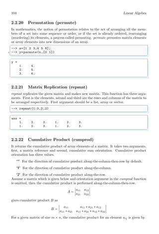
Roots of Polynomials
Roots of higher degree polynomials can be obtained as
✞
1 --> x=poly (0,’x’)
--> roots(x^3 - 6 * x^2 + 11 * x -6)
✌
✆
✞
ans =
3.
2.
1.
✌
✆
All are the real roots. roots function also calculates the complex roots.
✞
--> x=poly (0,’x’)
2 --> roots(x^3 - 6 * x^2 + 11 * x + 1)
✌
✆
✞
ans =
3.04 + 1.50 i
3.04 - 1.50 i
- 0.08
✌
✆
roots returns all the roots of a polynomial function. Roots of a polynomial function
are those possible values which satisfy to the given polynomial to zero. For example,
x2
− 2x + 1 = 0 is a polynomial of degree ‘2’ and is known as quadratic equation. The
roots of this polynomial are x = +1 and x = +1. When in place of ‘x’, 1 is put then
polynomial value is zero.
p(1) = 12
− 2 × 1 + 1 = 0
Roots of a polynomial is obtained either by fraction method or by substitution and re-
duction method.
✞
--> p=poly ([1,2,3], ’s’)
2 --> roots(p)
✌
✆
✞
ans =
3.
2.
1.
✌
✆](https://image.slidesharecdn.com/scilab-xcosprogrammingnotesforbeginners2-211010170430/85/Think-Like-Scilab-and-Become-a-Numerical-Programming-Expert-Notes-for-Beginners-2-of-2-by-Arun-Umrao-2-320.jpg)
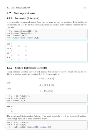
![2.2. ALGEBRA 103
2.2.18 Simplification (simp)
simp simplifies rational function. It returns numerator & denominator as result. This
functions takes two inputs as its arguments. First argument is numerator of algebraic
function and second argument is denominator of the algebraic function. For example,
assume a polynomial rational fraction
f =
(s + 1) ∗ (s + 2)
(s + 1) ∗ (s − 2)
On simplification of it, the result is
f =
s + 2
s − 2
Scilab code for this function is given below:
✞
--> s=poly (0,’s’);
2 --> [n,d]= simp ((s+1) *(s+2) ,(s+1)*(s-2))
✌
✆
✞
d =
- 2 + s
n =
2 + s
✌
✆
2.2.19 Flip Matrix Dimension (flipdim)
flipdim function flips the matrix with respect to the dimension as specified in the function.
It is similar to the row or column interchange in the matrix during solving of a problem.
Consider a matrix A as given below:
A =](https://image.slidesharecdn.com/scilab-xcosprogrammingnotesforbeginners2-211010170430/85/Think-Like-Scilab-and-Become-a-Numerical-Programming-Expert-Notes-for-Beginners-2-of-2-by-Arun-Umrao-3-320.jpg)


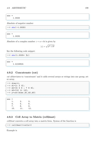
![See the example as given below:
✞
--> x=[1 2 3 4; 5 6 7 8]
2 --> dim =1;
--> y=flipdim (x,dim)
✌
✆
✞
x =
1. 2. 3. 4.
5. 6. 7. 8.
y =
5. 6. 7. 8.
1. 2. 3. 4.
✌
✆](https://image.slidesharecdn.com/scilab-xcosprogrammingnotesforbeginners2-211010170430/85/Think-Like-Scilab-and-Become-a-Numerical-Programming-Expert-Notes-for-Beginners-2-of-2-by-Arun-Umrao-19-320.jpg)
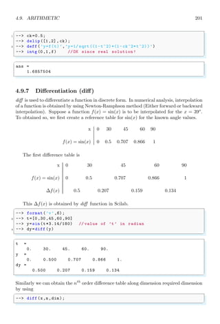
![104 Linear Algebra
2.2.20 Permutation (permute)
In mathematics, the notion of permutation relates to the act of arranging all the mem-
bers of a set into some sequence or order, or if the set is already ordered, rearranging
(reordering) its elements, a process called permuting. permute permutes matrix elements
or array elements into new dimensions of an array.
✞
--> x=[1 2 3;4 5 6];
2 --> y=permute (x,[2 1])
✌
✆
✞
y =
1. 4.
2. 5.
3. 6.
✌
✆
2.2.21 Matrix Replication (repmat)
repmat replicates the given matrix and makes new matrix. This function has three argu-
ments. First is the elements, second and third are the rows and columns of the matrix to
be arranged respectively. First argument should be a list, array or vector.
✞
--> repmat (1:3 ,2 ,2)
✌
✆
✞
ans =
1. 2. 3. 1. 2. 3.
1. 2. 3. 1. 2. 3.
✌
✆
2.2.22 Cumulative Product (cumprod)
It returns the cumulative product of array elements of a matrix. It takes two arguments,
first, a matrix reference and second, cumulative sum orientation. Cumulative product
orientation has three values.
‘*’ For the direction of cumulative product along-the-column-then-row by default.
‘1’ For the direction of cumulative product along-the-column.
‘2’ For the direction of cumulative product along-the-row.
Assume a matrix which is given below and orientation argument in the cumprod function
is omitted, then the cumulative product is performed along-the-column-then-row.
A =](https://image.slidesharecdn.com/scilab-xcosprogrammingnotesforbeginners2-211010170430/85/Think-Like-Scilab-and-Become-a-Numerical-Programming-Expert-Notes-for-Beginners-2-of-2-by-Arun-Umrao-20-320.jpg)


![2.2. ALGEBRA 105
✞
1 /* Perform cumulative product columnwise for an element */
for (l = 0; l < n; l++) {// columns
3 if (l < j) {
/* All row elements of previous columns */
5 for (k = 0; k < m; k++) {
r *= a[k][l];
7 }
} else if (l == j) {
9 /* Row element of current col at and before this row*/
for (k = 0; k <= i; k++) {
11 r *= a[k][l];
}
13 }
}
✌
✆
The example for cumulative product is given below:
✞
--> A=[1 ,2;3 ,4];
2 --> a=cumprod (A)
✌
✆
✞
a =
1. 6.
4. 10.
✌
✆
The same matrix which is given above is supplied to the cumprod function along with
second argument ‘1’, then the cumulative product is performed along-the-column.
A =](https://image.slidesharecdn.com/scilab-xcosprogrammingnotesforbeginners2-211010170430/85/Think-Like-Scilab-and-Become-a-Numerical-Programming-Expert-Notes-for-Beginners-2-of-2-by-Arun-Umrao-37-320.jpg)


![The example for cumulative product is given below:
✞
1 --> A=[1 ,2;3 ,4];
--> b=cumprod (A,1)
✌
✆
✞
b =
1. 2.
4. 6.
✌
✆
Second argument in the function cumprod is orientation of cumulative product. The
possible values are ‘1’ for right orientation and ‘2’ for center orientation. Similarly, the
same matrix is supplied to the cumprod function along with second argument ‘2’, then
the cumulative product is performed along-the-rows.
A =](https://image.slidesharecdn.com/scilab-xcosprogrammingnotesforbeginners2-211010170430/85/Think-Like-Scilab-and-Become-a-Numerical-Programming-Expert-Notes-for-Beginners-2-of-2-by-Arun-Umrao-53-320.jpg)


![For a given matrix of size m × n, the cumulative sum for an element aij is given by
✞
1 /* Perform cumulative sum columnwise for an element */
for (l = 0; l < n; l++) {// columns
3 if (l < j) {
/* All row elements of previous columns */
5 for (k = 0; k < m; k++) {
r += a[k][l];
7 }
} else if (l == j) {
9 /* Row elementd of current col at and before this row*/
for (k = 0; k <= i; k++) {
11 r += a[k][l];
}
13 }
}
✌
✆
The example for cumulative product is given below:
✞
--> A=[1 ,2;3 ,4];
2 --> a=cumsum(A)
✌
✆
✞
a =
1. 6.
4. 10.
✌
✆](https://image.slidesharecdn.com/scilab-xcosprogrammingnotesforbeginners2-211010170430/85/Think-Like-Scilab-and-Become-a-Numerical-Programming-Expert-Notes-for-Beginners-2-of-2-by-Arun-Umrao-86-320.jpg)


![The example for cumulative product is given below:
✞
1 --> A=[1 ,2;3 ,4];
--> b=cumsum(A,1)
✌
✆
✞
b =
1. 2.
4. 6.
✌
✆
Second argument in the function is orientation of cumulative sum. The possible values
are ‘1’ for right orientation and ‘2’ for center orientation. Similarly, the same matrix is
supplied to the cumsum function along with second argument ‘2’, then the cumulative
sum is performed along-the-rows.
A =](https://image.slidesharecdn.com/scilab-xcosprogrammingnotesforbeginners2-211010170430/85/Think-Like-Scilab-and-Become-a-Numerical-Programming-Expert-Notes-for-Beginners-2-of-2-by-Arun-Umrao-103-320.jpg)


![✞
1 --> A=[1 ,2;3 ,4];
--> kron (A,A)
✌
✆
✞
ans =
1. 2. 2. 4.
3. 4. 6. 8.
3. 6. 4. 8.
9. 12. 12. 16.
✌
✆](https://image.slidesharecdn.com/scilab-xcosprogrammingnotesforbeginners2-211010170430/85/Think-Like-Scilab-and-Become-a-Numerical-Programming-Expert-Notes-for-Beginners-2-of-2-by-Arun-Umrao-135-320.jpg)


![A Scilab example is given below:
✞
1 --> A=[1 ,2;3 ,4];
--> a=prod (A)
3 --> b=prod (A,1)
--> c=prod (A,2)
✌
✆
✞
a =
24.
b =
3. 8.
c =
2.
12.
✌
✆](https://image.slidesharecdn.com/scilab-xcosprogrammingnotesforbeginners2-211010170430/85/Think-Like-Scilab-and-Become-a-Numerical-Programming-Expert-Notes-for-Beginners-2-of-2-by-Arun-Umrao-172-320.jpg)


![A Scilab example is given below:
✞
1 --> A=[1 ,2;3 ,4];
--> a=sum(A)
3 --> b=sum(A,1)
--> c=sum(A,2)
✌
✆
✞
a =
10.
b =
4. 6.
c =
3.
7.
✌
✆](https://image.slidesharecdn.com/scilab-xcosprogrammingnotesforbeginners2-211010170430/85/Think-Like-Scilab-and-Become-a-Numerical-Programming-Expert-Notes-for-Beginners-2-of-2-by-Arun-Umrao-209-320.jpg)
![110 Linear Algebra
2.3 Matrices
A matrix is arrangement of coefficients of a set of algebraic equations in rows and columns.
Each row represents to a distinct algebraic equation while each column represents to
the coefficients of same variable of each equation. For example, take a set of algebraic
equations
ax + by = p; cx + dy = q
The coefficients of this set of algebraic equation shall be arranged in matrix form as
a b
c d
x
y
=
q
q
The word “matrix” refers only to the arrangement of coefficients of x and y variables
only. So, matrix is
a b
c d
First row has coefficients of equation ax + by = p and second row has coefficients of
equation cx + dy = q. First column has coefficients of variable x and second column
has coefficients of variable y. The number of rows is equal to the number of algebraic
equation in the given set and number of columns is equal to the number of distinct
variables. Numerical computational software have deep rooted application of matrices
or matrix structure. Thus we must have familiarity with matrices, their operations and
reading/writing matrix elements. Before, explaining the matrix operations, we will discuss
here about the reading/writing of matrix elements. For this purpose we take experimental
matrix
A =
1 2 3
4 5 6
7 8 9
✞
1 -- A=[1 2 3; 4 5 6; 7 8 9]
✌
✆
✞
A =
1. 2. 3.
4. 5. 6.
7. 8. 9.
✌
✆
Elements of matrix can be accessed by supplying indices in two ways. (i) have only one
argument, i.e. element-wise and (ii) have two arguments for row and column indices each
separated by comma. First argument is for rows and second argument is for columns. In
Scilab, indices starts from ‘1’ not from ‘0’. For example, if only one argument is supplied
as
✞
-- A(1:4)
✌
✆
Then it will return elements column-wise, i.e. from top to bottom in first column and
then second column and so on.](https://image.slidesharecdn.com/scilab-xcosprogrammingnotesforbeginners2-211010170430/85/Think-Like-Scilab-and-Become-a-Numerical-Programming-Expert-Notes-for-Beginners-2-of-2-by-Arun-Umrao-210-320.jpg)

![112 Linear Algebra
✞
ans =
1. 4. 7.
2. 5. 8.
3. 6. 9.
✌
✆
Two or more matrices can be added, subtracted, multiplied and divided if matrices follow
respective rules. If A, B and C are three matrices of order n × n then sum of all the
matrices is
Sij = Aij + Bij + Cij
✞
-- A=[1 ,2 ,3;4 ,5 ,6;7 ,8 ,9]
2 -- B=[5 ,6 ,7;8 ,9 ,10;11 ,12 ,13]
-- C=[10 ,11 ,12;13 ,14 ,15;16 ,17 ,18]
4 -- S=A+B+C
✌
✆
✞
A =
1. 2. 3.
4. 5. 6.
7. 8. 9.
B =
5. 6. 7.
8. 9. 10.
11. 12. 13.
C =
10. 11. 12.
13. 14. 15.
16. 17. 18.
S =
16. 19. 22.
25. 28. 31.
34. 37. 40.
✌
✆
Similarly subtraction of the two matrices can be obtained.
Dij = Aij − Bij
✞
-- A=[1 ,2 ,3;4 ,5 ,6;7 ,8 ,9]
2 -- B=[5 ,6 ,7;8 ,9 ,10;11 ,12 ,13]
-- D=A-B
✌
✆
✞
A =
1. 2. 3.
4. 5. 6.
7. 8. 9.
B =
5. 6. 7.
8. 9. 10.
11. 12. 13.](https://image.slidesharecdn.com/scilab-xcosprogrammingnotesforbeginners2-211010170430/85/Think-Like-Scilab-and-Become-a-Numerical-Programming-Expert-Notes-for-Beginners-2-of-2-by-Arun-Umrao-212-320.jpg)
![2.3. MATRICES 113
D =
- 4. - 4. - 4.
- 4. - 4. - 4.
- 4. - 4. - 4.
✌
✆
Sum and difference of the matrices are elementwise operations, hence matrices undergoing
addition and subtraction must be of same order. Product of the matrices is of two
type. (i) Dot (scalar) product and (ii) Cross (vector) product. Dot product or scalar
product is elementwise operation. It gives resultant matrix by multiplying elements by
elements. Due to elementwise operation, matrix addition, dot product are commutative.
Subtraction of matrices is not commutative as 2−3 6= 3−2. The dot product of matrices
symbol is group of dot and asterisk symbol (.*).
Pij = Aij. ∗ Bij
Example of dot product is given below:
✞
-- A=[1 ,2 ,3;4 ,5 ,6;7 ,8 ,9]
2 -- B=[5 ,6 ,7;8 ,9 ,10;11 ,12 ,13]
-- P=A.*B
✌
✆
✞
A =
1. 2. 3.
4. 5. 6.
7. 8. 9.
B =
5. 6. 7.
8. 9. 10.
11. 12. 13.
P =
5. 12. 21.
32. 45. 60.
77. 96. 117.
✌
✆
Cross product is special operation of the product of matrix. For cross product, number
of rows of one matrix must be equal to the number of columns of the other matrix.
A = [1, 2]; B =
3
4
The product A × B is possible. Using cross product rules, the result is
C = [1, 2] ×
3
4
= [11]
✞
-- A=[1 ,2]
2 -- B=[3;4]
-- C=A*B
✌
✆](https://image.slidesharecdn.com/scilab-xcosprogrammingnotesforbeginners2-211010170430/85/Think-Like-Scilab-and-Become-a-Numerical-Programming-Expert-Notes-for-Beginners-2-of-2-by-Arun-Umrao-213-320.jpg)
![114 Linear Algebra
✞
A =
1. 2.
B =
3.
4.
C =
11.
✌
✆
If this rule is not followed then Scilab shows error of inconsistent multiplication. Let we
have two matrices A and B as
A = [1, 2]; B = [3, 4]
✞
1 -- A=[1 ,2]
-- B=[3 ,4]
3 -- C=A*B
✌
✆
✞
A =
1. 2.
B =
3. 4.
C=AB
!--error 10
Inconsistent multiplication .
✌
✆
Cross product may or may not commutative. Most of matrices gives A× B 6= B × A. Let
two matrices are A and B of order n × n then
A
B
=
A
B
×
B−1
B−1
=
A × B−1
I
= A × B−1
Here, cross product of matrix and its inverse matrix is identity matrix. Note that dot
product of a matrix and its inverse matrix is not equal to identity matrix. See the following
Scilab codes for the division of the matrices.
✞
1 -- A=[1 ,2;3 ,4] //a 2x2 matrix
-- B=[5 ,6;7 ,8] //a 2x2 matrix
3 -- r=A/B // division of matrix p by matrix q
-- s=inv(B) // inverse of matrix q
5 -- t=A*s // cross product of p and inverse of q
✌
✆
✞
A =
1. 2.
3. 4.
B =
5. 6.
7. 8.
r =](https://image.slidesharecdn.com/scilab-xcosprogrammingnotesforbeginners2-211010170430/85/Think-Like-Scilab-and-Become-a-Numerical-Programming-Expert-Notes-for-Beginners-2-of-2-by-Arun-Umrao-214-320.jpg)


Think Like Scilab and Become a Numerical Programming Expert- Notes for Beginners 2 of 2 by Arun Umrao
- 1. 2.2. ALGEBRA 101 ✞ ans = 1 ✌ ✆ Again, changing the function Q2 = 2 − 3s, we have f(s) = 1 s3 ∗ (2 − 3s) Expanding the relation f(s) = 1 2s3 + 3 4s2 + 9 8s + 27 16 + 81 32 s + . . . The coefficient b1, i.e. the numeric coefficient of 1/s is called the residue of the function. Here, it is 1.125. ✞ --> s=poly (0,’s’); 2 --> P=1; --> Q1=s^3; 4 --> Q2 =(2 -3*s); --> residu(p, Q1 , Q2) ✌ ✆ ✞ ans = 1.125 ✌ ✆ 2.2.17 Roots of Polynomial (roots) Roots of a polynomial are those values which on substituted in place of variable gives polynomial value zero. A polynomial having degree of ‘n’ has n roots. Root values may be real numbers (either integers or fractions) or complex numbers. Roots of Quadratic Equation An equation of variable ‘x’ having degree ‘2’ is known as quadratic equation. Roots of the quadratic equation (Eg ax2 + bx + c = 0) can be obtained by using Shridharacharys Formula x = −b ± √ b2 − 4ac 2a Scilab example is given below ✞ --> x=poly (0,’x’) 2 --> roots(x^2 -3 * x + 2) ✌ ✆ ✞ ans = 2. 1. ✌ ✆ All the roots are real in integers. If equation is modified then roots becomes
- 2. 102 Linear Algebra ✞ 1 --> x=poly (0,’x’) --> roots(x^2 -3 * x + 3) ✌ ✆ ✞ ans = 1.5 + 0.8660254 i 1.5 - 0.8660254 i ✌ ✆ Roots of Polynomials Roots of higher degree polynomials can be obtained as ✞ 1 --> x=poly (0,’x’) --> roots(x^3 - 6 * x^2 + 11 * x -6) ✌ ✆ ✞ ans = 3. 2. 1. ✌ ✆ All are the real roots. roots function also calculates the complex roots. ✞ --> x=poly (0,’x’) 2 --> roots(x^3 - 6 * x^2 + 11 * x + 1) ✌ ✆ ✞ ans = 3.04 + 1.50 i 3.04 - 1.50 i - 0.08 ✌ ✆ roots returns all the roots of a polynomial function. Roots of a polynomial function are those possible values which satisfy to the given polynomial to zero. For example, x2 − 2x + 1 = 0 is a polynomial of degree ‘2’ and is known as quadratic equation. The roots of this polynomial are x = +1 and x = +1. When in place of ‘x’, 1 is put then polynomial value is zero. p(1) = 12 − 2 × 1 + 1 = 0 Roots of a polynomial is obtained either by fraction method or by substitution and re- duction method. ✞ --> p=poly ([1,2,3], ’s’) 2 --> roots(p) ✌ ✆ ✞ ans = 3. 2. 1. ✌ ✆
- 3. 2.2. ALGEBRA 103 2.2.18 Simplification (simp) simp simplifies rational function. It returns numerator & denominator as result. This functions takes two inputs as its arguments. First argument is numerator of algebraic function and second argument is denominator of the algebraic function. For example, assume a polynomial rational fraction f = (s + 1) ∗ (s + 2) (s + 1) ∗ (s − 2) On simplification of it, the result is f = s + 2 s − 2 Scilab code for this function is given below: ✞ --> s=poly (0,’s’); 2 --> [n,d]= simp ((s+1) *(s+2) ,(s+1)*(s-2)) ✌ ✆ ✞ d = - 2 + s n = 2 + s ✌ ✆ 2.2.19 Flip Matrix Dimension (flipdim) flipdim function flips the matrix with respect to the dimension as specified in the function. It is similar to the row or column interchange in the matrix during solving of a problem. Consider a matrix A as given below: A =
- 7. 1 2 3 4
- 11. When this matrix is flipped about first row, then flipped matrix becomes B as: B =
- 15. 3 4 1 2
- 19. See the example as given below: ✞ --> x=[1 2 3 4; 5 6 7 8] 2 --> dim =1; --> y=flipdim (x,dim) ✌ ✆ ✞ x = 1. 2. 3. 4. 5. 6. 7. 8. y = 5. 6. 7. 8. 1. 2. 3. 4. ✌ ✆
- 20. 104 Linear Algebra 2.2.20 Permutation (permute) In mathematics, the notion of permutation relates to the act of arranging all the mem- bers of a set into some sequence or order, or if the set is already ordered, rearranging (reordering) its elements, a process called permuting. permute permutes matrix elements or array elements into new dimensions of an array. ✞ --> x=[1 2 3;4 5 6]; 2 --> y=permute (x,[2 1]) ✌ ✆ ✞ y = 1. 4. 2. 5. 3. 6. ✌ ✆ 2.2.21 Matrix Replication (repmat) repmat replicates the given matrix and makes new matrix. This function has three argu- ments. First is the elements, second and third are the rows and columns of the matrix to be arranged respectively. First argument should be a list, array or vector. ✞ --> repmat (1:3 ,2 ,2) ✌ ✆ ✞ ans = 1. 2. 3. 1. 2. 3. 1. 2. 3. 1. 2. 3. ✌ ✆ 2.2.22 Cumulative Product (cumprod) It returns the cumulative product of array elements of a matrix. It takes two arguments, first, a matrix reference and second, cumulative sum orientation. Cumulative product orientation has three values. ‘*’ For the direction of cumulative product along-the-column-then-row by default. ‘1’ For the direction of cumulative product along-the-column. ‘2’ For the direction of cumulative product along-the-row. Assume a matrix which is given below and orientation argument in the cumprod function is omitted, then the cumulative product is performed along-the-column-then-row. A =
- 24. a11 a12 a21 a22
- 28. gives cumulative product B as B =
- 32. a11 a11 ∗ a21 ∗ a12 a11 ∗ a21 a11 ∗ a21 ∗ a12 ∗ a22
- 36. For a given matrix of size m × n, the cumulative product for an element aij is given by
- 37. 2.2. ALGEBRA 105 ✞ 1 /* Perform cumulative product columnwise for an element */ for (l = 0; l < n; l++) {// columns 3 if (l < j) { /* All row elements of previous columns */ 5 for (k = 0; k < m; k++) { r *= a[k][l]; 7 } } else if (l == j) { 9 /* Row element of current col at and before this row*/ for (k = 0; k <= i; k++) { 11 r *= a[k][l]; } 13 } } ✌ ✆ The example for cumulative product is given below: ✞ --> A=[1 ,2;3 ,4]; 2 --> a=cumprod (A) ✌ ✆ ✞ a = 1. 6. 4. 10. ✌ ✆ The same matrix which is given above is supplied to the cumprod function along with second argument ‘1’, then the cumulative product is performed along-the-column. A =
- 41. a11 a12 a21 a22
- 45. gives cumulative product B as B =
- 49. a11 a12 a11 ∗ a21 a12 ∗ a22
- 53. The example for cumulative product is given below: ✞ 1 --> A=[1 ,2;3 ,4]; --> b=cumprod (A,1) ✌ ✆ ✞ b = 1. 2. 4. 6. ✌ ✆ Second argument in the function cumprod is orientation of cumulative product. The possible values are ‘1’ for right orientation and ‘2’ for center orientation. Similarly, the same matrix is supplied to the cumprod function along with second argument ‘2’, then the cumulative product is performed along-the-rows. A =
- 57. a11 a12 a21 a22
- 62. 106 Linear Algebra gives cumulative product B as B =
- 66. a11 a11 ∗ a12 a21 a21 ∗ a22
- 70. 2.2.23 Cumulative Summation (cumsum) It returns the cumulative sum of array elements of a matrix. It takes two arguments, first, a matrix reference and second, cumulative summation orientation. Cumulative summation orientation has three values. ‘*’ For the direction of cumulative sum along-the-column-then-row by default. ‘1’ For the direction of cumulative sum along-the-column. ‘2’ For the direction of cumulative sum along-the-row. Assume a matrix which is given below, and orientation argument in the cumsum function is omitted, then the cumulative sum is performed along-the-column-then-row. A =
- 74. a11 a12 a21 a22
- 78. gives cumulative sum B as B =
- 82. a11 a11 + a21 + a12 a11 + a21 a11 + a21 + a12 + a22
- 86. For a given matrix of size m × n, the cumulative sum for an element aij is given by ✞ 1 /* Perform cumulative sum columnwise for an element */ for (l = 0; l < n; l++) {// columns 3 if (l < j) { /* All row elements of previous columns */ 5 for (k = 0; k < m; k++) { r += a[k][l]; 7 } } else if (l == j) { 9 /* Row elementd of current col at and before this row*/ for (k = 0; k <= i; k++) { 11 r += a[k][l]; } 13 } } ✌ ✆ The example for cumulative product is given below: ✞ --> A=[1 ,2;3 ,4]; 2 --> a=cumsum(A) ✌ ✆ ✞ a = 1. 6. 4. 10. ✌ ✆
- 87. 2.2. ALGEBRA 107 The same matrix which is given above is supplied to the cumsum function along with second argument ‘1’, then the cumulative sum is performed along-the-column. A =
- 91. a11 a12 a21 a22
- 95. gives cumulative sum B as B =
- 99. a11 a12 a11 + a21 a12 + a22
- 103. The example for cumulative product is given below: ✞ 1 --> A=[1 ,2;3 ,4]; --> b=cumsum(A,1) ✌ ✆ ✞ b = 1. 2. 4. 6. ✌ ✆ Second argument in the function is orientation of cumulative sum. The possible values are ‘1’ for right orientation and ‘2’ for center orientation. Similarly, the same matrix is supplied to the cumsum function along with second argument ‘2’, then the cumulative sum is performed along-the-rows. A =
- 107. a11 a12 a21 a22
- 111. gives cumulative sum B as B =
- 115. a11 a11 + a12 a21 a21 + a22
- 119. 2.2.24 Kronekar Product (kron) kron is a Kronekar product of a matrix. A matrix A of order 2 × 2 is A =
- 123. a11 a12 a21 a22
- 127. kron of this matrix is given by δ =
- 131. a11A a12A a21A a22A
- 135. ✞ 1 --> A=[1 ,2;3 ,4]; --> kron (A,A) ✌ ✆ ✞ ans = 1. 2. 2. 4. 3. 4. 6. 8. 3. 6. 4. 8. 9. 12. 12. 16. ✌ ✆
- 136. 108 Linear Algebra 2.2.25 Product (prod) prod returns the product of an array of elements of a matrix. Second argument to this function is the orientation of the product. If orientation argument is not provided then prod returns the product of all elements mutually. If product orientation argument is ‘1’ then product is performed along the column and if product orientation argument is ‘2’ then product is performed along the row. Product of a matrix, without orientation argument, is performed is shown below: A =
- 140. a11 a12 a21 a22
- 144. gives cumulative product as a = a11 ∗ a21 ∗ a12 ∗ a22 Product of a matrix, with orientation argument ‘1’, is performed is shown below: A =
- 148. a11 a12 a21 a22
- 152. gives cumulative product as a =
- 154. a11 ∗ a21 a12 ∗ a22
- 156. Product of a matrix, with orientation argument ‘2’, is performed is shown below: A =
- 160. a11 a12 a21 a22
- 164. gives cumulative product as a =
- 168. a11 ∗ a12 a21 ∗ a22
- 172. A Scilab example is given below: ✞ 1 --> A=[1 ,2;3 ,4]; --> a=prod (A) 3 --> b=prod (A,1) --> c=prod (A,2) ✌ ✆ ✞ a = 24. b = 3. 8. c = 2. 12. ✌ ✆
- 173. 2.2. ALGEBRA 109 2.2.26 Summation (sum) sum returns the sum of elements of a given matrix. Second argument to this function is the orientation of the summation. If summation orientation argument is ‘1’ then summation is performed along the column and if summation orientation argument is ‘2’ then summation is performed along the row. Summation of a matrix, without orientation argument, is performed is shown below: A =
- 177. a11 a12 a21 a22
- 181. gives cumulative summation as a = a11 + a21 + a12 + a22 Summation of a matrix, with orientation argument ‘1’, is performed is shown below: A =
- 185. a11 a12 a21 a22
- 189. gives cumulative summation as a =
- 191. a11 + a21 a12 + a22
- 193. Summation of a matrix, with orientation argument ‘2’, is performed is shown below: A =
- 197. a11 a12 a21 a22
- 201. gives cumulative summation as a =
- 205. a11 + a12 a21 + a22
- 209. A Scilab example is given below: ✞ 1 --> A=[1 ,2;3 ,4]; --> a=sum(A) 3 --> b=sum(A,1) --> c=sum(A,2) ✌ ✆ ✞ a = 10. b = 4. 6. c = 3. 7. ✌ ✆
- 210. 110 Linear Algebra 2.3 Matrices A matrix is arrangement of coefficients of a set of algebraic equations in rows and columns. Each row represents to a distinct algebraic equation while each column represents to the coefficients of same variable of each equation. For example, take a set of algebraic equations ax + by = p; cx + dy = q The coefficients of this set of algebraic equation shall be arranged in matrix form as a b c d x y = q q The word “matrix” refers only to the arrangement of coefficients of x and y variables only. So, matrix is a b c d First row has coefficients of equation ax + by = p and second row has coefficients of equation cx + dy = q. First column has coefficients of variable x and second column has coefficients of variable y. The number of rows is equal to the number of algebraic equation in the given set and number of columns is equal to the number of distinct variables. Numerical computational software have deep rooted application of matrices or matrix structure. Thus we must have familiarity with matrices, their operations and reading/writing matrix elements. Before, explaining the matrix operations, we will discuss here about the reading/writing of matrix elements. For this purpose we take experimental matrix A = 1 2 3 4 5 6 7 8 9 ✞ 1 -- A=[1 2 3; 4 5 6; 7 8 9] ✌ ✆ ✞ A = 1. 2. 3. 4. 5. 6. 7. 8. 9. ✌ ✆ Elements of matrix can be accessed by supplying indices in two ways. (i) have only one argument, i.e. element-wise and (ii) have two arguments for row and column indices each separated by comma. First argument is for rows and second argument is for columns. In Scilab, indices starts from ‘1’ not from ‘0’. For example, if only one argument is supplied as ✞ -- A(1:4) ✌ ✆ Then it will return elements column-wise, i.e. from top to bottom in first column and then second column and so on.
- 211. 2.3. MATRICES 111 ✞ ans = 1. 4. 7. 2. 5. ✌ ✆ If two arguments are supplied as ✞ -- A(1:1 ,2:2) ✌ ✆ Then it will return elements from row one to row one and from column two to column two. Thus it will only return element ‘2’. ✞ ans = 2. ✌ ✆ If column range is changed from column two to column three, then output will be changed. ✞ -- A(1:1 ,2:3) // First row and 2nd and 3rd columns ✌ ✆ ✞ ans = 2. 3. ✌ ✆ For row or column access, respective row or column index is provided and other argument is supplied as range operator ‘:’. ✞ -- A(1,:) // First row and all columns ✌ ✆ ✞ ans = 1. 2. 3. ✌ ✆ ✞ -- A(:,2) // All rows and second columns ✌ ✆ ✞ ans = 2. 5. 8. ✌ ✆ There are several types of matrices. The most common type of matrix is square matrix. In square matrix, rows and columns are of equal size. ✞ -- x=1:1:9; 2 -- matrix(x,3,3) ✌ ✆
- 212. 112 Linear Algebra ✞ ans = 1. 4. 7. 2. 5. 8. 3. 6. 9. ✌ ✆ Two or more matrices can be added, subtracted, multiplied and divided if matrices follow respective rules. If A, B and C are three matrices of order n × n then sum of all the matrices is Sij = Aij + Bij + Cij ✞ -- A=[1 ,2 ,3;4 ,5 ,6;7 ,8 ,9] 2 -- B=[5 ,6 ,7;8 ,9 ,10;11 ,12 ,13] -- C=[10 ,11 ,12;13 ,14 ,15;16 ,17 ,18] 4 -- S=A+B+C ✌ ✆ ✞ A = 1. 2. 3. 4. 5. 6. 7. 8. 9. B = 5. 6. 7. 8. 9. 10. 11. 12. 13. C = 10. 11. 12. 13. 14. 15. 16. 17. 18. S = 16. 19. 22. 25. 28. 31. 34. 37. 40. ✌ ✆ Similarly subtraction of the two matrices can be obtained. Dij = Aij − Bij ✞ -- A=[1 ,2 ,3;4 ,5 ,6;7 ,8 ,9] 2 -- B=[5 ,6 ,7;8 ,9 ,10;11 ,12 ,13] -- D=A-B ✌ ✆ ✞ A = 1. 2. 3. 4. 5. 6. 7. 8. 9. B = 5. 6. 7. 8. 9. 10. 11. 12. 13.
- 213. 2.3. MATRICES 113 D = - 4. - 4. - 4. - 4. - 4. - 4. - 4. - 4. - 4. ✌ ✆ Sum and difference of the matrices are elementwise operations, hence matrices undergoing addition and subtraction must be of same order. Product of the matrices is of two type. (i) Dot (scalar) product and (ii) Cross (vector) product. Dot product or scalar product is elementwise operation. It gives resultant matrix by multiplying elements by elements. Due to elementwise operation, matrix addition, dot product are commutative. Subtraction of matrices is not commutative as 2−3 6= 3−2. The dot product of matrices symbol is group of dot and asterisk symbol (.*). Pij = Aij. ∗ Bij Example of dot product is given below: ✞ -- A=[1 ,2 ,3;4 ,5 ,6;7 ,8 ,9] 2 -- B=[5 ,6 ,7;8 ,9 ,10;11 ,12 ,13] -- P=A.*B ✌ ✆ ✞ A = 1. 2. 3. 4. 5. 6. 7. 8. 9. B = 5. 6. 7. 8. 9. 10. 11. 12. 13. P = 5. 12. 21. 32. 45. 60. 77. 96. 117. ✌ ✆ Cross product is special operation of the product of matrix. For cross product, number of rows of one matrix must be equal to the number of columns of the other matrix. A = [1, 2]; B = 3 4 The product A × B is possible. Using cross product rules, the result is C = [1, 2] × 3 4 = [11] ✞ -- A=[1 ,2] 2 -- B=[3;4] -- C=A*B ✌ ✆
- 214. 114 Linear Algebra ✞ A = 1. 2. B = 3. 4. C = 11. ✌ ✆ If this rule is not followed then Scilab shows error of inconsistent multiplication. Let we have two matrices A and B as A = [1, 2]; B = [3, 4] ✞ 1 -- A=[1 ,2] -- B=[3 ,4] 3 -- C=A*B ✌ ✆ ✞ A = 1. 2. B = 3. 4. C=AB !--error 10 Inconsistent multiplication . ✌ ✆ Cross product may or may not commutative. Most of matrices gives A× B 6= B × A. Let two matrices are A and B of order n × n then A B = A B × B−1 B−1 = A × B−1 I = A × B−1 Here, cross product of matrix and its inverse matrix is identity matrix. Note that dot product of a matrix and its inverse matrix is not equal to identity matrix. See the following Scilab codes for the division of the matrices. ✞ 1 -- A=[1 ,2;3 ,4] //a 2x2 matrix -- B=[5 ,6;7 ,8] //a 2x2 matrix 3 -- r=A/B // division of matrix p by matrix q -- s=inv(B) // inverse of matrix q 5 -- t=A*s // cross product of p and inverse of q ✌ ✆ ✞ A = 1. 2. 3. 4. B = 5. 6. 7. 8. r =
- 215. 2.3. MATRICES 115 3. - 2. 2. - 1. s = - 4. 3. 3.5 - 2.5 t = 3. - 2. 2. - 1. ✌ ✆ 2.3.1 Determinant The determinant det(A) or |A| of a square matrix A is a number encoding certain prop- erties of the matrix. A matrix is invertible if and only if its determinant is nonzero. Determinant of the matrix A =
- 221. a b c d e f g h i
- 227. is given by |A| = a(e × i − h × f) − b(d × i − g × f) + c(d × h − g × e) It is a numerical value and crucial for the solution of the given algebraic equations or matrix. Scilab example is ✞ 1 -- det ([2 ,3 ,5;8 ,1 ,5;9 ,7 ,2]) ✌ ✆ ✞ ans = 256. ✌ ✆ 2.3.2 Transpose Matrix Transpose matrix is the change of rows into columns and vice versa of a square matrix. ✞ -- x=1:1:9; 2 -- y=matrix(x,3,3),y’ ✌ ✆ ✞ y = 1. 4. 7. 2. 5. 8. 3. 6. 9. ans = 1. 2. 3. 4. 5. 6. 7. 8. 9. ✌ ✆
- 228. 116 Linear Algebra 2.3.3 Diagonal Matrix A matrix which has only non-zero diagonal elements and other elements are zero, is called diagonal matrix. Mathematically A = aij when i = j 0 when i 6= j In Scilab diagonal matrix is ✞ -- diag ([1 ,2 ,3]) // elements in [] are diagonal elements . ✌ ✆ ✞ ans = 1. 0. 0. 0. 2. 0. 0. 0. 3. ✌ ✆ 2.3.4 Identity Matrix Identity matrix has only unity diagonal elements and other elements are zeros. Mathe- matically I = aij = 1 when i = j = 0 when i 6= j In Scilab identity matrix is ✞ -- eye (2,3)// eye(row , columns) ✌ ✆ ✞ ans = 1. 0. 0. 0. 1. 0. ✌ ✆ The product of a matrix and identity matrix is that matrix, i.e. A × I = I × A = A 2.3.5 Inverse of Matrix From the definition of inverse, if x is a number and y is its inverse then x × y = 1. Similarly, if P is a invertible square matrix and P−1 is its inverse then PP−1 = I Where I is unit identity matrix having same order as the matrix P has. A matrix should be square matrix for being invertible. All square matrices are not invertible. The square matrix which has an inverse is called invertible or non-singular matrix. A square matrix is invertible when its determinant is not zero, i.e. det(A) 6= 0. Inverse of a square matrix is given by A−1 = Adj(A) Det(A)
- 229. 2.3. MATRICES 117 Adj(A) of the matrix A is transpose matrix of the co-factor matrix of matrix A. Co-factor of a matrix of m × n order in respect of ith row and jth column is given by Aij that is equal to the product of (−1)i×j and determinant of remaining matrix after eliminating ith row and jth column. Let a matrix is given like A = 1 2 3 4 The co-factors of the matrix are a11 = (−1)1×1 × 4 a11 = (−1)1×2 × 3 a21 = (−1)2×1 × 2 a22 = (−1)2×2 × 1 Now co-factors matrix of matrix A is Acf = 4 −3 −2 1 Now Adj(A) of matrix A is Adj(A) = 4 −2 −3 1 Now the determinant of the matrix A is Det(A) = −2 Finally, inverse of matrix A is A−1 = Adj(A) Det(A) = −2 1 1.5 −0.5 Inverse of a 3 × 3 square matrix P = 1 3 5 4 8 9 2 1 6 is find by using Scilab as ✞ 1 -- P=[1 ,3 ,5;4 ,8 ,9;2 ,1 ,6] -- inv(P) ✌ ✆ ✞ ans = - 1. 0.3333333 0.3333333 0.1538462 0.1025641 - 0.2820513 0.3076923 - 0.1282051 0.1025641 ✌ ✆
- 230. 118 Linear Algebra 2.3.6 Normalization of Matrix A matrix T is said to be normalized if T 2 = I where, I is identity matrix. Take a matrix A as A =
- 234. a b c d
- 238. Let k is factor that must be multiply to matrix A such that, T = kA and kA × kA = I. Now, kA × kA shall be transform in such manner that A2 = KI. Now the new form of the matrix is k2 A2 = I. It give k2 KI = I Or k = 1 √ K Now, the normalized matrix is T = kA, which gives T 2 = I. Take a matrix A =
- 242. 3 2 −2 −3
- 246. Its A2 is A × A =
- 250. 5 0 0 5
- 254. This matrix can be transformed in form of KI as shown below: A × A = 5 ×
- 258. 1 0 0 1
- 262. Now, the value of k is 0.4472136. Now the transform matrix is T + kA T = kA =
- 270. See the Scilab example as given below: ✞ -- A = [3,2;-2,-3] 2 -- k = 1/5^0.5 -- N = k*A 4 -- N*N ✌ ✆ ✞ A = 3. 2. - 2. - 3. k = 0.4472136 N = 1.3416408 0.8944272 - 0.8944272 - 1.3416408
- 271. 2.3. MATRICES 119 ans = 1. 0. 0. 1. ✌ ✆ A matrix may or may not be normalized. 2.3.7 Normalzation Factor (norm) norm returns the normalized form of a matrix. A matrix T is said to be normalized if T 2 = I where, I is identity matrix. Take a matrix A as A =
- 275. a b c d
- 279. Let k is factor that must be multiply to matrix A such that, T = kA and kA × kA = I. Now, kA × kA shall be transform in such manner that A2 = KI. Now the new form of the matrix is k2 A2 = I. It give k2 KI = I The norm function returns the value of K associated with a matrix, i.e. ✞ -- K=norm (A) ✌ ✆ Further proceeding successive steps for finding of the normalized matrix. k = 1 √ K Now, the normalized matrix is T = kA which givens T 2 = I. Take a matrix A =
- 283. 3 2 −2 −3
- 287. Its A2 is A × A =
- 291. 5 0 0 5
- 295. This matrix can be transformed in form of KI as shown below: A × A = 5 ×
- 299. 1 0 0 1
- 303. Now, the value of k is 0.4472136. Now the transform matrix is T + kA T = kA =
- 311. See the Scilab example as given below: ✞ 1 -- A=[3,2;-2,-3]; -- k=1/ norm (A)^0.5 3 -- N=k*A -- N*N ✌ ✆
- 312. 120 Linear Algebra ✞ A = 3. 2. - 2. - 3. k = 0.4472136 N = 1.3416408 0.8944272 - 0.8944272 - 1.3416408 ans = 1. 0. 0. 1. ✌ ✆ There are following types of normalization of a matrix. Norm Type Description norm(x,2) Largest singular value of x. It is com- puted like (max(svd(x))) norm(x,1) The l 1 norm x. It is sum of largest column. Its value is max(sum(abs(x), ‘r′ )). norm(x,‘inf’) The infinity norm of x. It is computed by max(sum(abs(x), ‘c′ )). norm(x,‘fro’) Frobenius norm. Computed by sqrt(sum(diag(x′ ∗ x))) for a vector. norm(v,p) The l p norm. It is computed from re- lation (sum(v(i)p ))(1/p) . 2.3.8 Permutation Transposition (pertrans) pertrans is the permutation and transposition of the elements of a matrix simultaneously. Take a matrix A =
- 316. 1 2 3 3 4 4
- 320. Its permutation and transposition, rows are transform into columns and then columns are arranged from right to left in matrix form. For example, the permutation and trans- position of matrix, A is B (say) B =
- 326. 4 3 4 2 3 1
- 332. ✞ -- A = [1 ,2 ,3;3 ,4 ,4]; 2 -- pertrans (A) ✌ ✆
- 333. 2.3. MATRICES 121 ✞ ans = 4. 3. 4. 2. 3. 1. ✌ ✆ Similarly, the permutation and transposition of matrix A =
- 341. 1 2 3 3 4 4 7 6 8 0 9 8
- 349. is B (say) B =
- 355. 8 8 4 3 9 6 4 2 0 7 3 1
- 361. ✞ -- A = [1 ,2 ,3;3 ,4 ,4;7 ,6 ,8;0 ,9 ,8]; 2 -- pertrans (A) ✌ ✆ ✞ ans = 8. 8. 4. 3. 9. 6. 4. 2. 0. 7. 3. 1. ✌ ✆ 2.3.9 Orthogonal Matrix An orthogonal matrix is a square matrix with real entries whose columns and rows are orthogonal unit vectors. Equivalently, a matrix A is orthogonal if its transpose is equal to its inverse: AT = A−1 We can find the orthogonal matrix of a given matrix by decomposing it as explained in function svd. It is equal to the Matrix U of the svd decomposition. ✞ -- orth ([1 ,2;3 ,4]) ✌ ✆ ✞ ans = - 0.4045536 - 0.9145143 - 0.9145143 0.4045536 ✌ ✆ 2.3.10 Complex Matrix Complex matrix is a matrix whose at least one element is a complex number. A complex numbers are written in form of z = a + ib. A real number is also a complex number with zero imaginary part, i.e. z = 2 + i0. The function complex accepts two matrices of equal shape and size as its argument. First matrix represents real part of the complex number, while second matrix represents to the imaginary part of the complex numbers.
- 362. 122 Linear Algebra ✞ 1 -- // First part is real , second part is imaginary -- complex ([1 2;3 4],[3 4;5 8]) ✌ ✆ ✞ ans = 1. + 3.i 2. + 4.i 3. + 5.i 4. + 8.i ✌ ✆ 2.3.11 Matrix Product Vector product of two matrices (different from elementwise product) is performed by special mathematical operations. Matrix product is possible, if number of rows in left matrix is equal to the number of columns in right matrix. Let we have two matrices of equal size 2 × 2 as given below: A =
- 366. a b c d
- 370. ; B =
- 374. e f g h
- 378. The vector product of the matrices is given by C = A × B as Cij = mn X ij AijBji Here corresponding elements of columns of right matrix are multiplied by respective elements of rows of left matrix and their respective products are added with each other. The vector product of matrices A and B is A × B =
- 382. ae + bg af + bh ce + dg cf + dh
- 386. ✞ 1 -- a=[1 ,3 ,5;4 ,8 ,9;2 ,1 ,6]; -- b=[1 ,3 ,5;4 ,8 ,9;2 ,1 ,6]; 3 -- a*b ✌ ✆ ✞ ans = 23. 32. 62. 54. 85. 146. 18. 20. 55. ✌ ✆ Scalar matrix product (element-wise matrix product) is performed by multiplying corre- sponding elements of the two matrices. Scalar product is possible if both matrices are of equal size. The scalar matrix product of two matrices is given by C = A · B as Cij = Aij · Bij Assume two matrices A =
- 390. a b c d
- 394. ; B =
- 398. e f g h
- 403. 2.3. MATRICES 123 The element-wise matrix product of these two matrices is A · B =
- 407. ae bf cg dh
- 411. ✞ -- a=[1 ,3 ,5;4 ,8 ,9;2 ,1 ,6]; 2 -- b=[1 ,3 ,5;4 ,8 ,9;2 ,1 ,6]; -- a.*b ✌ ✆ ✞ ans = 1. 9. 25. 16. 64. 81. 4. 1. 36. ✌ ✆ 2.3.12 Eigenvalues of Matrix An eigenvector of a square matrix A is a non-zero vector v that, when the matrix is multiplied by v, yields a constant multiple of v, the multiplier being commonly denoted by λ. That is: Av = λv The number λ is called the eigenvalue of A corresponding to Av. To find the eigenvalues, we solve above relations as Av − λv = 0 ⇒ (A − λI)v = 0 To get the values of λ we will solve the relation A − λI. Note that, v can not be equal to zero. So, A − λI must be zero. Matrix equation will be found if determinant of A − λI is equal to zero. |A − λI| = 0 Expand the determinants and find all the values of λ. Values of λ are eigenvalues of the given matrix. Assume a matrix A as A = 1 2 3 4 For its eigenvalues, we have
- 415. 1 2 3 4 − λ 1 0 0 1
- 419. = 0 Or
- 423. 1 − λ 2 3 4 − λ
- 427. = 0 It gives λ2 − 5λ − 2 = 0 On solving it, we have λ = −0.37 and λ = 5.37. The Scilab codes are
- 428. 124 Linear Algebra ✞ -- spec ([1 ,2;3 ,4]) // eigenvectors ✌ ✆ ✞ ans = - 0.3722813 5.3722813 ✌ ✆ 2.3.13 Triangular Lower Matrix (tril) tril returns the lower triangular matrix. If a matrix is given like A = a f g f b h g h c Now the lower triangular matrix of matrix A is A = a 0 0 f b 0 g h c ✞ 1 -- s=poly (0,’s’); -- tril ([s,s;s,1]) ✌ ✆ ✞ ans = s 0 s 1 ✌ ✆ 2.3.14 Triangular Upper Matrix (triu) tril returns the upper triangular matrix. If a matrix is given like A = a f g f b h g h c Now the lower triangular matrix of matrix A is A = a f g 0 b h 0 0 c ✞ -- s=poly (0,’s’); 2 -- triu ([s,s;s,1]) ✌ ✆
- 429. 2.3. MATRICES 125 ✞ ans = s s 0 1 ✌ ✆ 2.3.15 Lower Upper Matrix (lu) This function factorize a given matrix in lower triangular and upper triangular matrices. It is used as ✞ -- [L,U,E]=lu(matrix name ); ✌ ✆ Where input matrix is m×n real or complex matrix. L is lower triangular real or complex matrix of size m × min(m, n) and U is upper triangular real or complex matrix of size min(m, n) × n. E is a n × n permutation matrix. ✞ 1 -- A=[1 ,3;2 ,1] -- [L,U,E]=lu(A) ✌ ✆ ✞ E = 0. 1. 1. 0. U = 2. 1. 0. 2.5 L = 1. 0. 0.5 1 ✌ ✆ 2.3.16 Diagonal Matrix (diag) For a matrix A =
- 435. a b c d e f g h i
- 441. The diagonal elements are given as d = [a, e, i]. This function returns the diagonals of a matrix or diagonal matrix. Diagonal elements are taken along the main diagonal of the matrix. Its syntax is ✞ 1 -- diag ( matrix name ) ✌ ✆ Take a matrix A of size 3 × 3 A =
- 447. 1. 2. 3. 4. 1. 5. 8. 8. 9.
- 454. 126 Linear Algebra The diagonals of the matrix ‘A’ is d =
- 460. 1. 1. 9.
- 466. If matrix name supplied to this function is of m × 1 size then it convert it into the matrix of m×m size with all the input elements at the diagonals of the output matrix. Elements other than diagonal are sets to zero. Take input matrix of type d =
- 472. 1. 1. 9.
- 478. Then diagonal matrix shall be D =
- 484. 1. 0. 0. 0. 1. 0. 0. 0. 9.
- 490. Scilab example is ✞ 1 -- A=[1, 2, 3; 4, 1, 5; 8, 8, 9] -- d=diag (A) ✌ ✆ ✞ A = 1. 2. 3. 4. 1. 5. 8. 8. 9. d = 1. 1. 9. ✌ ✆ The diagonal matrix is constructed from the diagonals of the given matrix ‘A’ by using the diag() function. ✞ 1 -- D=diag (d) ✌ ✆ ✞ D = 1. 0. 0. 0. 1. 0. 0. 0. 9. ✌ ✆ If a matrix is not a square matrix, then rows and columns from the top-left position are chosen, which ultimately form a perfect square matrix. For example, if a non-square matrix is A =
- 498. 1. 2. 3. 4. 1. 5. 8. 8. 9. 4. 8. 5.
- 507. 2.3. MATRICES 127 then diag() function assumes the given matrix as A =
- 516. 1. 2. 3. 4. 1. 5. 8. 8. 9. . . . ... . . ..
- 525. for extraction of diagonal from the given matrix. The diagonal of the matrix ‘A’ is obtained by using diag() function as d =
- 531. 1. 1. 9.
- 537. Here elements are taken along the main diagonal of the matrix. 2.3.17 Jordan Canonical Form (bdiag) It is also called diagonalization of a matrix. A matrix is said to be diagonalizable if it can be transform into Jordan canonical (normal) form as given below: A = P · D · P−1 Where D is diagonal matrix. Matrix function can be used with diagonalized matrix as f(A) = P · f(D) · P−1 Here, matrix function is operated only with diagonal matrix not with P or P−1 . For example, suppose a matrix A as A = 1 3 2 1 It can be transformed into P · D · P−1 form as A = P 0.344 0 0 −1.449 # P−1 Where P = 0.774 −0.790 0.632 0.645 Now, the matrix function operation, for example inverse of matrix A is given as A−1 = P · D−1 · P−1 And solving above relation by substituting the values of P, D we get A−1 and it is A−1 = −0.2 0.6 0.4 −0.2
- 538. 128 Linear Algebra ✞ -- A=[1 ,3;2 ,1]; 2 -- [D,P,d]= bdiag(A) ✌ ✆ ✞ d = 1. 1. P = 0.7745967 - 0.7905694 0.6324555 0.6454972 D = 3.4494897 0. 0. - 1.4494897 ✌ ✆ Here, d is diagonals of the matrix A. On computation of P · D · P−1 ), we get the matrix A. ✞ 1 -- P*D*inv(P) ✌ ✆ ✞ ans = 1. 3. 2. 1. ✌ ✆ Applying the inverse matrix operation, we get the same result by P ·D−1 ·P−1 ) and A−1 . ✞ 1 -- I=P*inv(D)*inv(P) -- i=inv(A) ✌ ✆ ✞ I = - 0.2 0.6 0.4 - 0.2 i = - 0.2 0.6 0.4 - 0.2 ✌ ✆ 2.3.18 Cholensky Factorization (chol) The Cholesky decomposition of a Hermitian positive-definite matrix A, is a decomposition of the form A = LL ′ where L is a lower triangular matrix with real and positive diagonal entries, and L∗ denotes the conjugate transpose of L. A positive-definite matrix has positive determinant.
- 539. 2.3. MATRICES 129 Scilab function chol is used for the cholensky factorization of a matrix. Let we have a matrix 3 2 3 4 Its determinant is |A| = 12 − 6 = 6 0. So, it is positive-definite matrix. Now, The A = LL ′ decomposition is 3 2 3 4 = 1.7320508 0. 1.1547005 1.6329932 1.7320508 1.1547005 0. 1.6329932 ✞ 1 --A=[3 ,2;3 ,4] --chol (A) ✌ ✆ ✞ A = 3. 2. 3. 4. ans = 1.7320508 1.1547005 0. 1.6329932 ✌ ✆ Every Hermitian positive-definite matrix has a unique Cholesky decomposition. Let we have a Hermitian matrix A = 4 2 + 2i 2 − 2i 3 Its determinant |A| 0, hence it has Cholesky decomposition. Scilab codes for this matrix are given below: ✞ 1 -- A=[4 ,2+2* %i ;2-2*%i ,3] -- R=chol (x) ✌ ✆ ✞ A = 4. 2. + 2.i 2. - 2.i 3. R = 2. 1. + i 0. 1. ✌ ✆ 2.3.19 Determinant of Matrix (det) det returns the determinant of a square vector matrix. If a matrix is given like A = 1 2 3 4 5 6 7 8 9
- 540. 130 Linear Algebra Then, determinant of this matrix A is |A| = 1(45 − 48) − 2(36 − 42) + 3(32 − 35) = 0 Hence determinant of the matrix A is zero. Scilab call of determinant of the matrix is ✞ 1 -- det ([1 ,2 ,3;4 ,5 ,6;7 ,8 ,9]) ✌ ✆ ✞ ans = 6.661D-16 ✌ ✆ 2.3.20 Inverse Matrix (inv) inv returns the inverse of a square matrix. Inverse of a matrix can be obtained if it is convertible. All square matrices are not convertible. The square matrix which has an inverse is called convertible or non-singular matrix. A square matrix is convertible when its determinant is not zero, i.e. det(A) 6= 0. If A is a matrix then A × A−1 = I i.e. vector product of matrix and its inverse matrix is unitary matrix. Dot product of matrix and its inverse matrix is not unitary matrix. ✞ -- A=[1 ,2;3 ,4] // Matrix of 2x2 order 2 -- B=A*inv(A) // Cross product of matrix and its inverse -- C=A.* inv(A) // Dot product of matrix and its inverse ✌ ✆ ✞ A = 1. 2. 3. 4. B = 1. 0. 8.882D-16 1. C = - 2. 2. 4.5 - 2. ✌ ✆ Inverse of a square matrix is given by A−1 = Adj(A) Det(A) Adj(A) of the matrix A is transpose matrix of the co-factor matrix of matrix A. Co-factor of a matrix of m × n order in respect of ith row and jth column is given by Aij that is
- 541. 2.3. MATRICES 131 equal to the product of (−1)i×j and determinant of remaining matrix after eliminating ith row and jth column. Let a matrix is given like A = 1 2 3 4 The co-factors of the matrix are a11 = (−1)1×1 × 4; a11 = (−1)1×2 × 3; a21 = (−1)2×1 × 2; a22 = (−1)2×2 × 1; Now co-factors matrix of matrix A is Acf = 4 −3 −2 1 Now Adj(A) of matrix A is Adj(A) = 4 −2 −3 1 Now the determinant of the matrix A is Det(A) = −2 Finally, inverse of matrix A is A−1 = Adj(A) Det(A) = −2 1 1.5 −0.5 This result can be obtained by calling Scilab function inv like ✞ -- inv ([1 ,2;3 ,4]) ✌ ✆ ✞ ans = - 2. 1. 1.5 - 0.5 ✌ ✆ 2.3.21 Orthogonal Matrix (orth) In linear algebra, an orthogonal matrix is a square matrix whose columns and rows are orthogonal unit vectors (orthonormal vectors). Orthogotal matrix is represented as AT A = AAT = I Where, AT is transpose of the matrix A. I is identity matrix. From the relation A−1 A = AA−1 = I we can say that a matrix A is orthogonal if its transpose is equal to its inverse, i.e. AT = A−1 . For example, 1 0 0 1 0.96 −0.28 0.28 0.96
- 542. 132 Linear Algebra An orthogonal basis for an inner product space V is a basis for V whose vectors are mutually orthogonal. If the vectors of an orthogonal basis are normalized, the resulting basis is an orthonormal basis. In Scilab, orth returns the orthogonal basis of a given matrix. To illustrate method of orth function, consider a matrix A = a b c d where, u = a c v = b d The orthogonal basis for first column shall be found by dividing all column elements by column normalisation value as shown in below matrix. c1 = a √ a2 + c2 c √ a2 + c2 Second column is calculated by using relation c2 = v − u · v u · u × u Or c2 = b d − ab + cd a2 + b2 × a c Now, divide all elements of second columns by column normalisation value. The orthog- onal basis shall be matrix constructed with columns c1 and c2. ✞ 1 B=orth (A) ✌ ✆ returns an orthonormal basis for the range of A. The columns of B span the same space as the columns of A, and the columns of B are orthogonal, so that BT ∗ B = eye(rank(A)). The number of columns of B is the rank of A. Take matrix A = 3 2 1 2 where, u = 3 1 v = 2 2 The orthogonal basis for first column shall be found by dividing all column elements by column normalisation value as shown in below matrix. c1 = 3 √ 32 + 12 = 0.948683298 1 √ 32 + 12 = 0.316227766 Second column is calculated by using relation c2 = 2 2 − 3 × 2 + 1 × 2 32 + 12 × 3 1 This gives c2 = −0.4 1.2
- 543. 2.3. MATRICES 133 Dividing it with normalised column value, we get c2 = −0.4 p (−0.4)2 + 1.22 = −0.316227766 1.2 p (−0.4)2 + 1.22 = 0.948683298 The orthogonal basis shall be matrix constructed with columns c1 and c2. c2 = 0.948683298 −0.316227766 0.316227766 0.948683298 ✞ 1 -- A= [3 2;1 2] -- orth (A) ✌ ✆ ✞ ans = - 0.8649101 - 0.5019268 - 0.5019268 0.8649101 ✌ ✆ This result is different from what we have calculated. This is due to different way of Gram-Schmidt Orthonormal Method implementation. Orthogonal basis implementation of above illustrated method in scilab script is shown below: ✞ 1 -- function A = myOrth(A) -- k=size (A,2); 3 -- function w = proj (u,v) -- w = (sum(v.*u)/sum(u.*u)) * u; 5 -- endfunction -- for r = 1:1: k 7 -- A(:,r) = A(:,r) / norm (A(:,r)) -- for c = r+1:1:k 9 -- ; u v -- A(:,c) = A(:,c) - proj (A(:,r),A(:,c)) 11 -- end -- end 13 -- endfunction -- A = [3 ,2;1 ,2] 15 -- myOrth(A) ✌ ✆ 2.3.22 Rank of Matrix (rank) rank determines the minimum non-zero rows of a matrix when reduces to echelon form. Suppose a matrix A is in echelon form as A = 1 0 0 1
- 544. 134 Linear Algebra and it has two non zero rows. Now the rank of matrix is 2. Similarly, rank of following matrix B = 1 2 0 0 0 1 0 0 0 is also two. Rank of a matrix can be obtained by Scilab by using function rank function like ✞ 1 -- rank ([1, 0; 0, 1]) ✌ ✆ ✞ ans = 2. ✌ ✆ Example with other matrix of 3 × 3 order: ✞ -- rank ([1 ,3 ,5;4 ,8 ,9;2 ,1 ,6]) ✌ ✆ ✞ ans = 3. ✌ ✆ 2.3.23 Eigenvalues Eigenvectors (spec) spec evaluates eigenvalues and eigenvectors of a square matrix. The eigenvalues of a matrix is given by |A − λI| = 0 Assume a matrix of order 2 × 2 A = 1 2 3 4 Now its eigenvalues are given by |A − λI| = 0 ie
- 548. 1 2 3 4 − λ 1 0 0 1
- 552. = 0 Or
- 556. 1 − λ 2 3 4 − λ
- 560. = 0 Or (1 − λ) × (4 − λ) − 6 = 0 On solving it λ = −0.372281; 5.372281 Or eigenvalues in matrix form, when they are arranged in descending order is d = 5.372281 0.000000 0.000000 −0.372281
- 561. 2.3. MATRICES 135 For λ = 5.372281, eigenvector (v1) is (A − λI)v1 = 0. So, 1 − 5.372281 2 3 4 − 5.372281 x y = 0 −4.372281 2 3 −1.372281 x y = 0 Or −4.372281x + 2y = 0; 3x − 1.372281y = 0 To get solutions, put x = 1 in −4.372281x + 2y = 0, we get the value of y = 2.186140. To get eigenvectors, we shall normalize these two values as x = 1 √ 12 + 2.1861402 ; y = 2.186140 √ 12 + 2.1861402 It gives, x = 0.415973 and y = 0.909376. As coefficients of above two eigenvector equa- tions are of opposite signs, hence values of x and y shall be either both negative or both positive. Now, we shall submit x and y values in equation g = 3x − 1.372281y to get minimum positive value. g = 3 × 0.415973 − 1.372281 × 0.909376 = 0.000000407 Taking sign convention, the other possible set of solution be x = −0.415973 and y = −0.909376. g = 3 × −0.415973 − 1.372281 × −0.909376 = 0.000000407 When x = −0.415973 and y = −0.909376, we have positive f value. This gives first eigenvector corresponding to λ = 5.372281. v1 = −0.415973 −0.909376 We can also find normalized x and y solution from 3x − 1.372281y = 0 and minimum positive value of f = −4.372281x+2y can be found by substituting x and y values taking sign conventions. For λ = −0.372281, eigenvector (v2) is (A − λI)v2 = 0. So, 1 − (−0.372281) 2 3 4 − (−0.372281) x y = 0 1.372281 2 3 4.372281 x y = 0 Or 1.372281x + 2y = 0; 3x + 4.372281y = 0 As coefficients of above two eigenvector equations are of same signs, hence values of x and y shall be in opposite signs. On solving these two algebraic equations, as explained for λ = 5.372281, we have x = −0.824564 and y = 0.565767 or x = 0.824564 and y =
- 562. 136 Linear Algebra −0.565767. From the numberline, acceptable values are x = −0.824564 and y = 0.565767. This gives second eigenvector corresponding to λ = −0.372281. v2 = −0.824564 0.565767 The corresponding eigenvector matrix from above two eigenvectors (v1 and v2) is v = −0.415973 −0.824564 −0.909376 0.565767 From Scilab, eigenvalues and eigenvectors are obtained by using function spec like ✞ -- [vec , val]= spec ([1 ,2; 3,4]) ✌ ✆ ✞ val = - 0.3722813 0 0 5.3722813 vec = - 0.8245648 - 0.4159736 0.5657675 - 0.9093767 ✌ ✆ 2.3.24 Square Root of Matrix Assume a matrix of order 2 × 2 A = 1 2 3 4 Now its eigenvalues are given by |A − λI| = 0 i.e.
- 566. 1 2 3 4 − λ 1 0 0 1
- 570. = 0 Or
- 574. 1 − λ 2 3 4 − λ
- 578. = 0 Or (1 − λ) × (4 − λ) − 6 = 0 On solving it λ = −0.372281; 5.372281 Or eigenvalues in matrix form, when they are arranged in descending order is d = 5.372281 0.000000 0.000000 −0.372281 For λ = 5.372281, eigenvector (v1) is (A − λI)v1 = 0. So, 1 − 5.372281 2 3 4 − 5.372281 x y = 0
- 579. 2.3. MATRICES 137 −4.372281 2 3 −1.372281 x y = 0 Or −4.372281x + 2y = 0; 3x − 1.372281y = 0 To get solutions, put x = 1 in −4.372281x + 2y = 0, we get the value of y = 2.186140. To get eigenvectors, we shall normalize these two values as x = 1 √ 12 + 2.1861402 ; y = 2.186140 √ 12 + 2.1861402 It gives, x = 0.415973 and y = 0.909376. As coefficients of above two eigenvector equa- tions are of opposite signs, hence values of x and y shall be either both negative or both positive. Now, we shall submit x and y values in equation g = 3x − 1.372281y to get minimum positive value. g = 3 × 0.415973 − 1.372281 × 0.909376 = 0.000000407 Taking sign convention, the other possible set of solution be x = −0.415973 and y = −0.909376. g = 3 × −0.415973 − 1.372281 × −0.909376 = 0.000000407 When x = −0.415973 and y = −0.909376, we have positive f value. This gives first eigenvector corresponding to λ = 5.372281. v1 = −0.415973 −0.909376 For λ = −0.372281, eigenvector (v2) is (A − λI)v2 = 0. So, 1 − (−0.372281) 2 3 4 − (−0.372281) x y = 0 1.372281 2 3 4.372281 x y = 0 Or 1.372281x + 2y = 0; 3x + 4.372281y = 0 As coefficients of above two eigenvector equations are of same signs, hence values of x and y shall be in opposite signs. On solving these two algebraic equations, as explained for λ = 5.372281, we have x = −0.824564 and y = 0.565767 or x = 0.824564 and y = −0.565767. This gives second eigenvector corresponding to λ = −0.372281. v2 = −0.824564 0.565767 The corresponding eigenvector matrix from above two eigenvectors (v1 and v2) is v = −0.415973 −0.824564 −0.909376 0.565767
- 580. 138 Linear Algebra Note that, each column of eignevectors is arranged to the corresponding eigenvalues. Now, the matrix A can be written as A = v × d × v−1 . The square root of the matrix is given by A 1 2 = v × d 1 2 × v−1 ✞ -- A=[1 ,2; 3,4] 2 -- [vec , val]= spec (A) -- B=vec*sqrt (val)*inv(vec) 4 -- M=B*B ✌ ✆ ✞ A = 1. 2. 3. 4. val = - 0.372281 0 0 5.372281 vec = - 0.824564 - 0.415973 0.565767 - 0.909376 B = 0.553688 + 0.464394 i 0.806960 - 0.212426 i 1.210441 - 0.318639 i 1.764129 + 0.145754 i M = 1. + 1.110D-16i 2. + 4.163D-17i 3. + 8.327D-17i 4. ✌ ✆ Here, matrix M is same as matrix A. 2.3.25 Hermitian Factorisation (sqroot) A Hermitian matrix (A) (or self-adjoint matrix) is a complex square matrix that is equal to its own conjugate transpose (AT ). In other words, the ijth element of Hermitian matrix is equal to the complex conjugate of the jith element of Hermitian matrix for all indices i and j. Elements of a Hermitian matrix are satisfy aij = aji. If A is a Hermitian matrix then sqroot of matrix A returns a matrix B such that A = BBT .In Scilab, sqroot function is used to find the square root of the Hermitian matrix. ✞ -- A=[1 ,2;2 ,1] 2 -- B=sqroot(A) -- B*B’ ✌ ✆ ✞ A = 1. 2. 2. 1. B = - 1.2247449 0.7071068 - 1.2247449 - 0.7071068 ans =
- 581. 2.3. MATRICES 139 1. 2. 2. 1. ✌ ✆ 2.3.26 Signaular Matrix A matrix is said to be singular whose determinant is zero. A two dimensional singular matrix is A =
- 585. 1 1 1 1
- 589. Its determinant is |A| = 1 − 1 = 0. Inverse of a singular matrix is not possible as its determinant is zero. 2.3.27 Singular Value Approximation (sva) sva is acronym of Singular Value Approximation of a matrix. ✞ 1 -- sva ([1 ,2;3 ,4]) ✌ ✆ ✞ ans = -0.4045536 -0.9145143 -0.9145143 0.4045536 ✌ ✆ This returns left singular vectors of the given matrix. Mathematically, sva is matrix U of the Singular Value Decomposition (see svd). 2.3.28 Singular Value Decomposition (svd) svd acronym of Singular Value Decomposition of a matrix. Singular Value Decomposition (SVD) is a factorization of a real or complex matrix. Singular value decomposition of a rectangular matrix Am×n where m is rows represents genes and n is column represents the experimental conditions. The SVD theorem states than Am×n = Um×m Sm×n V T n×n Where U and V are orthogonal, i.e. UT U = Im×m and V T V = In×n. Here, the columns of U are the left singular vectors; S has singular values and is diagonal; and V T has rows that are the right singular vectors. SVD calculation consists 1. Eigenvalues and Eigenvectors of AAT and AT A. 2. Eigenvectors of AAT make up the columns of U. 3. The Eigenvectors of AT A make up the columns of V . 4. The singular values in S are square roots of eigenvalues from AAT or AT A.
- 590. 140 Linear Algebra The singular values are the diagonal entries of the S matrix and are arranged in descending order. The singular values are always real numbers. If the matrix A is a real matrix, then U and V are also real. Let a matrix A and its transpose matrix AT are respectively A = 1 2 3 4 AT = 1 3 2 4 Now, AAT is 1 2 3 4 1 3 2 4 = 5 11 11 25 Eigenvalues of this matrix is found when |AAT − λI| = 0. So,
- 594. 5 − λ 11 11 25 − λ
- 598. = (5 − λ)(25 − λ) − 121 = 0 This gives eigenvalues of the matrix AAT and eigenvalues are arranged in descending order. val = 29.866069 0.000000 0.000000 0.133931 and find the corresponding eigenvectors as
- 602. 5 − 29.866069 11 11 25 − 29.866069
- 606. x y = 0 It gives, −24.866069x + 11y = 0; 11x − 4.866069y = 0 The eigenvector (v1) corresponding to λ = 29.866069 is found by solving these two equa- tions. Recall the solutions of algebraic equations, these equations have only one solution, that is x = 0 and y = 0. This is true if we take x, y ∈ I. If x, y ∈ R, then we can approximate the values of x and y so that above algebraic equations are satisfied approxi- mately to zero, i.e. left hand side solution tends to zero. As x and y have “opposite sign” coefficients, therefore, values of x and y may be either both positive or both negative. To solve the relation, put x = 1 in −24.866069x + 11y = 0, we have −24.866069 × 1 + 11y = 0 This gives y = 2.260551. Normalizing these values we have, x = 1 √ 12 + 2.2605512 ; y = 2.260551 √ 12 + 2.2605512 Or x = 0.40455369; y = 0.914514249 Substituting these values in equation g = 11x − 4.866069y, we have g+ 1 = 11 × 0.40455369 − 4.866069 × 0.914514249 = −0.000001153 g− 1 = 11 × −0.404552907 − 4.866069 × −0.914514595 = 0.000001153
- 607. 2.3. MATRICES 141 Note that there are two equations for λ = 29.866069 therefore approximate values of x and y may be found either of the two equations. But here, we shall find x and y from each equation separately and their values will be put in other equation to check which solution set is more close to zero. Take x = 1, in 11x − 4.866069y = 0, we get the value of y 11 × 1 − 4.866069y = 0 This gives y = 2.260551587. Normalizing these values we have, x = 1 √ 2.2605515872 + 12 ; y = 2.260551587 √ 2.2605515872 + 12 Or x = 0.404553602; y = 0.914514288 Substituting values of x and y in equation f = −24.866069x + 11y, we have f+ 1 = −24.866069 × 0.404553602 + 11 × 0.914514288 = −0.000000614 f− 2 = −24.866069 × −0.404553602 + 11 × −0.914514288 = 0.000000614 Here, x = −0.40455369, y = −0.914514249, give minimum positive value. Why we consider minimum positive value? To understand it, consider modulo function f(x) = −x when x 0 x when x ≥ 0 It means 0 is positive side. That’s why, 0.000000614 is considered more closure to zero than −0.000000614. Hence acceptable eignevector is v1 = −0.404553 −0.914514 Now, we shall find the corresponding eigenvectors for eigenvalue λ = 0.133931.
- 611. 5 − 0.133931 11 11 25 − 0.133931
- 615. x y = 0 It gives, 4.866068x + 11y = 0; 11x + 24.866068y = 0 The eigenvector (v2) corresponding to λ = 0.133931 is found by solving these two equa- tions. Recall the solutions of algebraic equations, these equations have only one solution, that is x = 0 and y = 0. This is true if we take x, y ∈ I. If x, y ∈ R, then we can approximate the values of x and y so that above algebraic equations are satisfied approx- imately to zero, i.e. left hand side solution tends to zero. As x and y have “same sign” coefficients, therefore, values of x and y shall have opposite signs. We know that any number when multiplied by a constant |k| 1, i.e. −1 k +1, result approaches to zero as k → 0. So, that the solutions of these two equations shall be within (−1, +1). To solve the relation, take x = 1 in 4.866068x + 11y = 0, we have 4.866068 × 1 + 11y = 0
- 616. 142 Linear Algebra This gives y = −0.442369818. Normalizing these values we have, x = 1 p (−0.442369818)2 + 12 ; y = −0.442369818 p (−0.442369818)2 + 12 Or x = 0.914514319; y = −0.404553533 Substituting these values in equation g = 11x + 24.866068y, we have g+ 1 = 11 × 0.914514319 + 24.866068 × −0.404553533 = 0.000001848 g− 1 = 11 × −0.914514319 + 24.866068 × 0.404553533 = −0.000001848 To solve the second relation 11x + 24.866068y = 0, take x = 1, we have 11 × 1 + 24.866068y = 0 This gives y = −0.442369899. Normalizing these values we have, x = 1 p (−0.442369899)2 + 12 ; y = −0.442369899 p (−0.442369899)2 + 12 Or x = 0.914514291; y = −0.404553595 Substituting these values in equation f = 4.866068x + 11y, we have f+ 1 = 4.866068 × 0.914514291 + 11 × −0.404553595 = −0.000000818 f− 1 = 4.866068 × −0.914514291 + 11 × 0.404553595 = 0.000000818 The minimum positive value is obtained when x = −0.914514291 and y = 0.404553595. So, the eignevector is v2 = −0.914514 0.404553 Eigenvector of the matrix AAT is column arrangement of v1 and v2. vec = −0.404553 −0.914514 −0.914514 0.404553 Here, U = −0.404553 −0.914514 −0.914514 0.404553 Similarly, eigenvalues and eigenvectors of AT A shall be computed as computed for AAT above. The matrix relation AT A is 1 3 2 4 1 2 3 4 = 10 14 14 20 Eigenvalues of this matrix is found when |AT A − λI| = 0. So,
- 620. 10 − λ 14 14 20 − λ
- 624. = (10 − λ)(20 − λ) − 196 = 0
- 625. 2.3. MATRICES 143 This gives eigenvalues and corresponding eigenvectors as val = 29.866069 0.000000 0.000000 0.133931 ; vec = −0.576048 0.817415 −0.817415 −0.576048 Here, V = −0.576048 0.817415 −0.817415 −0.576048 S is the square root of the eigenvalues from AAT or AT A. So, S = √ 29.866069 0.000000 0.000000 √ 0.133931 = 5.464985 0.000000 0.000000 0.365966 Here, each column of val matrix represents the eignevalues of AAT or AT A matrices and corresponding columns of U or V are eigenvectors corresponding to the eigenvalues respectively. Relation between U, S and V with A as A = USV T Now, from the above explained example, the modified values of U, S and V are U = −0.404553 −0.914514 −0.914514 0.404553 V = −0.576048 0.817415 −0.817415 −0.576048 S = 5.464985 0.000000 0.000000 0.365966 In Scilab, svd of given matrix is given by ✞ 1 -- [U,S,V]= svd ([1 ,2;3 ,4]) ✌ ✆ This function has three outputs as given below: ✞ V = - 0.5760484 0.8174156 - 0.8174156 - 0.5760484 S = 5.4649857 0. 0. 0.3659662 U = - 0.4045536 - 0.9145143 - 0.9145143 0.4045536 ✌ ✆ 2.3.29 Trace of Matrix (trace) Tracing of a square matrix is sum of its diagonal elements. If A is a square matrix of order n × n then T r(A) = n X i=1 aii
- 626. 144 Calculus If λi are the eigenvalues of a matrix A, then tracing of the matrix is T r(A) = X i λi In Scilab, trace returns the tracing of a matrix. ✞ 1 -- A=rand (3,3) -- trace(A) ✌ ✆ ✞ A = 0.3312931 0.7221236 0.3707945 0.0518477 0.0774625 0.2116117 0.4149242 0.5855878 0.1903269 ans = 0.5990825 ✌ ✆
- 627. 3.1. DERIVATIVE CALCULUS 145 3Calculus 3.1 Derivative Calculus 3.1.1 Derivative Derivative of a function f(x) is given by f′ (x) = lim h→0 f(x + h) − f(x) h where, h is approximately zero but not zero. Symbolic derivative of a function in Scilab is calculated by derivat function. ✞ -- s=poly (0,’s’); 2 -- derivat (1/s) ✌ ✆ ans = −1 s2 derivative function calculates the numerical derivative of a function. ✞ -- function y=myF(x) 2 -- y = x*x; -- endfunction 4 -- x = 1; -- fp = derivative (myF ,x) ✌ ✆ ✞ fp = 2. ✌ ✆ 3.1.2 Numeric Derivative Second method of finding the derivative of a function is numdiff that is more accurate than the derivative function. Mathematically, it is given by numdiff (f)|x=c = df dx
- 631. x=c It always returns numeric value rather than symbolic output.
- 632. 146 Calculus ✞ -- function y=myF(x) 2 -- y = x*x; -- endfunction 4 -- x = 1; -- fp = numdiff(myF ,x) ✌ ✆ ✞ fp = 2. ✌ ✆ 3.1.3 Numeric Difference diff function is used to find the difference between two consecutive elements continuously. This function is used with a vector having only numeric values. In mathematics, first order discrete difference is given by ∆f = fn+1 − fn A function table and its first order difference is given in the following table. f = 1 8 27 64 125 216 ∆f = 7 19 37 61 91 The diff function does the same work. Numerically, it is reqpresented like diff(f) = fn+1 − fn ✞ -- v=(1:8) ^3; 2 -- diff (v) ✌ ✆ ✞ ans = 7. 19. 37. 61. 91. 127. 169. ✌ ✆ 3.1.4 Function Evaluation (feval) Multiple evaluation of a function for one or two arguments of vector type. The syntax is ✞ -- feval(var 1, var 2, ...., var n, n var func ) ✌ ✆ Example is ✞ 1 -- function [z]=f(x,y) -- z=x+y; 3 -- endfunction -- a=1:3; 5 -- b=1:3; -- feval(a,b,f) ✌ ✆
- 633. 3.2. INTEGRAL CALCULUS 147 ✞ ans = 2. 3. 4. 3. 4. 5. 4. 5. 6. ✌ ✆ 3.2 Integral Calculus 3.2.1 Integration Integration is also called anti-derivative. It is a method of finding reverse of differentiation. x y f(x) dx b x = a b x = b The symbolic representation of integral of a function is given by I = Z f(x)dx Where symbol Z represent to the integration. f(x) is function on which integration is to be performed and dx is the base in which d represents the small element of function and x the base variable against which integration is to be performed. Variables other than x are considered as constants. Indefinite integral has global scope while definite integral is computed within the given limits of independent variable. I = Z b a f(x)dx Scilab does not support symbolic integration but it has one of the most precisive calcu- lations in numerical integration i.e. definite integration. Integration of a simple function f(x) = x is ✞ --I=integrate (’x’,’x’ ,0,1) ✌ ✆ ✞ I = 0.5 ✌ ✆ In this integration command, first term is integrand function, second term is base variable, third is lower limit and fourth term is upper limit. Applying these observations, the integration of t2 is
- 634. 148 Calculus ✞ --I=integrate (’t*t’,’t’ ,0,1) ✌ ✆ ✞ I = 0.3333333 ✌ ✆ Similarly integration of a sine function is ✞ -- I=integrate (’sin(t)’,’t’ ,0,1) ✌ ✆ ✞ I = 0.4596977 ✌ ✆ Remember that lower limit and upper limit in trigonometric integration are taken by trigonometric functions in radian unit of angle. Definite integration of trigonometric function is computed by using intg function. ✞ -- function y=f(x) 2 -- y=sin(x)/x -- endfunction 4 -- I=intg (0,2*%pi ,f) ✌ ✆ ✞ I = 1.4181516 ✌ ✆ There are several method of finding the integration by interpolation method. One of them is Trapezoidal method. ✞ -- t=0:0.1: %pi; 2 -- inttrap (t,sin(t)) ✌ ✆ ✞ ans = 1.9974689 ✌ ✆ The quadrature method of integration is given by 3.2.2 Double Integral (int2d) Double integral is used to integrate a function along two dimensions. For example, double integral is given by A = Z Z f(x, y)dx dy where dx and dy are length and width of element in x-axis and y-axis. Double integral gives volume of region bounded between two axes and f(x, y).
- 635. 3.2. INTEGRAL CALCULUS 149 x y z f(x, y) dx dy int2d is used to integrate two dimensional functions. The syntax is ✞ -- [I,e]= int2d( .. 2 -- a three dimensional N array for abscissa , .. -- a three dimensional N array for ordinate , .. 4 -- external function .. -- ) ✌ ✆ Here I is integrated value and e is estimated error. Example is ✞ 1 -- function [z]=f(x,y) -- z=x+y; 3 -- endfunction -- X=[0 ,0;1 ,1;1 ,0]; 5 -- Y=[0 ,0;0 ,1;1 ,1]; -- int2d(X,Y,f) ✌ ✆ ✞ ans = 1. ✌ ✆ 3.2.3 Tripple Integration (int3d) int3d is used to integrate three dimensional functions. The syntax is ✞ -- [I,e]= int3d( .. 2 -- a four dimensional array for abscissae , .. -- a four dimensional array for ordinate , .. 4 -- a four dimensional array for z-axis , .. -- external function .. 6 -- ) ✌ ✆ Here I is integrated value and e is estimated error. ‘external function’ is a function or list or string which defines the integrand f(xyz, nf), where xyz is the vector of a point coordinates and nf is the number function. By default nf is 1. Example is ✞ -- function v=f(xyz , numfun) 2 -- v=xyz ’* xyz; -- endfunction 4 -- // Tetrahedron coordinates
- 636. 150 Calculus -- //(0,0,0) ,(1,0,0) ,(0,1,0) ,(0,0,1) 6 -- X=[0;1;0;0]; -- Y=[0;0;1;0]; 8 -- Z=[0;0;0;1]; -- [I,e]= int3d(X,Y,Z,f ,1) ✌ ✆ ✞ e = 5.551D-16 I = 0.05 ✌ ✆ Another example is ✞ -- function v=f(F, numfun) 2 -- //x+y+z=1 -- v=1; 4 -- endfunction -- // Tetrahedron coordinates 6 -- //(0,0,0) ,(1,0,0) ,(0,1,0) ,(0,0,1) -- X=[0;1;0;0]; // Vector of abscissa values 8 -- Y=[0;0;1;0]; // Vector of ordinate values -- Z=[0;0;0;1]; // Vector of z values 10 -- [I,e]= int3d(X,Y,Z,f ,1) ✌ ✆ ✞ e = 1.850D-15 I = 0.1666667 ✌ ✆ Another example is ✞ -- function v=f(F, numfun) 2 -- //x+y+z=6 -- v=6; 4 -- endfunction -- // tetrahedron coordinates 6 -- //(0,0,0) ,(2,0,0) ,(0,3,0) ,(0,0,1) -- X=[0;2;0;0]; // Vector of abscissa values 8 -- Y=[0;0;3;0]; // Vector of ordinate values -- Z=[0;0;0;1]; // Vector of z values 10 -- [I,e]= int3d(X,Y,Z,f ,1) ✌ ✆ ✞ e = 6.661D-14 I = 6. ✌ ✆
- 637. 3.2. INTEGRAL CALCULUS 151 3.2.4 Integrate (integrate) integrate function calculates the sum of values of a function for all the point range within the limits by using quadrature method. Plane integration is simple area bounded by function and the axis of limits. It is given by Z f(x) dx = n X i=0 f(xi) × h Where h is width of the two consecutive lower upper bound limits. ✞ -- x0 =0; 2 -- x1 =2; -- X= integrate (’sin(x)’, ’x’, x0 , x1) ✌ ✆ ✞ ans = 1.4161468 ✌ ✆ 3.2.5 Definite Integration (intg) It return the definite integration of an external function. If f(x) is a function bounded between close interval [a b] then definite integral of the function is given by I = Z b a f(x) dx Definite integration of given relation I = Z 2π 0 x sin(30x) q 1 − x 2π 2 dx is −2.5432. Now the Scilab call of definite integral of the above relation is ✞ -- function y=f(x) 2 -- y=x*sin (30* x)/sqrt (1-((x/(2* %pi))^2)) -- endfunction 4 -- I=intg (0,2*%pi ,f) ✌ ✆ ✞ ans = - 2.5432596 ✌ ✆ 3.2.6 Cauchy’s Integration (intc) If f is a complex-valued function, then intc computes the integral over the curve in the complex plane from lower limit z1 to upper limit z2 of the complex function f(z) along the line z1z2. Since line integrals of analytic functions are independent of the path, function intc can be used to evaluate integrals of any analytic function. Syntax of Cauchy’s Line integral is given below:
- 638. 152 Calculus ✞ -- [I,e]= intc (.. 2 -- var z1 ,.. // complex number -- var z2 ,.. // complex number 4 -- external function of two vars (f) .. -- ) ✌ ✆ Here I is integrated value and e is estimated error. Let z = x(t) + iy(t) is a parametric curve of t in complex plane C, where z1 ≤ t ≤ z2. Let f(z) is continuous function on complex plane C. 1 −1 1 2 −1 −2 x y b b b b b b b b b b b z0 z1 z2 zn−1 zn 1 −1 1 2 −1 −2 x y b b b b b b b b b b b z1 z2 ∆zi bc Si The t is sub divided into n subdivisions as a = t0, t1, . . ., tn = b and corresponding subdivisions of curve on C is z0, z1, . . ., zn. The width of two consecutive subdivisions of curve is ∆zi = zi − zi−1, where 0 i n. If function is continuous and limit exists over each subdivision of curve, then bounded area of curve within given bounded limits is sum of areas of all subdivisions. So, Sn = n X i=1 f(zi)∆zi Here, Sn is line integral of function f(z) and it is represented by I = Z C f(z) dz = Z z2 z1 f(z) dz Where dz = |∆zi| → 0. Scilab uses following relation for computation of complex integral in intc function. Z C f(z) dz = Z z2 z1 f(C(z))C′ (z) dz To parameterize this relation, put z = z1 + (z2 − z1)t. When z = z1, t = 0 and when z = z2, t = 1. This gives Z C f(z) dz = Z 1 0 f(z1 + (z2 − z1)t) (z2 − z1) dt Real and imaginary part of integrand are computed separately and their sum is desired result.
- 639. 3.2. INTEGRAL CALCULUS 153 Illustrated Example Take a function f(z) = i. We have to find Cauchy’s integral along the line za = 1 − i to zb = 1 + i. The Cauchy’s line integral for the curve shall be I = Z C f(z) dz = Z 1+i 1−i i dz I = [iz] 1+i 1−i = i [(1 + i) − (1 − i)] This gives I = i × 2i = 2i2 = −2 This is desired result. ✞ 1 -- function [I]=f(z) -- I=%i; 3 -- endfunction -- intc (1-%i ,1+%i ,f) ✌ ✆ ✞ ans = - 2 ✌ ✆ Illustrated Example Take a function f(z) = 1 + i. We have to find Cauchy’s integral along the line za = 1 − i to zb = 1 + i. The Cauchy’s line integral for the curve shall be I = Z C f(z) dz = Z 1+i 1−i (1 + i) dz I = [(1 + i)z] 1+i 1−i = (1 + i) [(1 + i) − (1 − i)] This gives I = (1 + i) × 2i = 2(−1 + i) This is desired result. ✞ -- function [I]=f(z) 2 -- I=1+%i; -- endfunction 4 -- intc (1-%i ,1+%i ,f) ✌ ✆ ✞ ans = - 2 + 2 i ✌ ✆ Illustrated Example Let the given function is f(z) = z2 . We have to integrate it along the line 0 to 1 + i in complex plane. The Cauchy’s line integral intc along the curve is given by Z C f(z) dz = Z 1+i 0 f(z) dz
- 640. 154 Calculus Parameterization of this integral, we will substitute z = z1 + (z2 − z1)t. When z = z1, t = 0 and when z = z2, t = 1. Again dz = (z2 − z1)dt Thus Z C f(z) dz = Z 1 0 (z1 + (z2 − z1)t)2 × (z2 − z1) dt Substituting the value of z1 and z2. Z C f(z) dz = Z 1 0 (1 + i)2 t2 × (1 + i) dt = Z 1 0 (1 + i)3 t2 dt Or Z C f(z) dz = (1 + i)3 t3 3
- 644. 1 0 = (1 + i)3 3 = 2i(1 + i) 3 This is desired result. The Scilab code for this example are ✞ -- function y=f(z) 2 -- y=z^2 -- endfunction 4 -- intc (0,1+%i ,f) ✌ ✆ ✞ ans = - 0.6666667 + 0.6666667 i ✌ ✆ 3.2.7 Cauchy Integration (intl) If f is a complex-valued function, then intl computes the integral of f(z) over the line in the complex plane, along the curve defined by z = z0 + reiθ for θ1 ≤ θ ≤ θ2 and |z − z0| ≤ r. The syntax of this function is ✞ -- [y]= intl ( .. 2 -- var a, .. // lower limit , real number -- var b, .. // upper limit , real number 4 -- origin point as complex number (z0), .. -- positive real number (r), .. 6 -- external function (f) .. -- ) ✌ ✆ Here, z0 is center of circle in complex plane and r is radius of the circle within exponential phase between θ1 and θ2. The Cauchy’s path integral of complex function f(z) dz along the curve C(θ) = z0 + reiθ is given by
- 645. 3.2. INTEGRAL CALCULUS 155 1 1 2 3 x f(x) z1 z2 θ1 θ2 1 1 2 3 x f(x) z1 z2 b b θ θ1 θ2 Z C f(z) dz = Z θ2 θ1 f(C(θ))C′ (θ) dθ Where, θ1 ≤ θ ≤ θ2. To convert it into parametric form, put θ = θ1 + (θ2 − θ1)t Now, when θ = θ1, t = 0 and when θ = θ2, t = 1. Thus the limit in parametric form is 0 ≤ t ≤ 1. This gives C(t) = z0 + rei[θ1+(θ2−θ1)t] and Z C f(z) dz = Z 1 0 f(C(t))C′ (t) dt Now, real and imaginary parts of the above relation are integrated separately and final result is equal to the sum of real and imaginary integrals. Scilab uses following intl codes. ✞ 1 -- function r=intl (a,b,z0 ,r,f) -- function y=real1(t) 3 -- z=r*exp(%i *((1-t)*a+t*b)) -- y=real (f(z+z0)*%i*(b-a)*z) 5 -- endfunction -- function y=imag1(t) 7 -- z=r*exp(%i *((1-t)*a+t*b)) -- y=imag (f(z+z0)*%i*(b-a)*z) 9 -- endfunction -- r=intg (0,1, real1)+%i*intg (0,1, imag1) 11 -- endfunction ✌ ✆ Illustrated Example Let the given function is f(z) = z2 . We have to integrate it along the unit circle, i.e. |z| = r ≤ 1 and 0 ≤ θ ≤ 2π. The Cauchy’s line integral intl along the curve is given by Z C f(z) dz = Z b a f(z) dz The curve of integral about z0 origin is z = z0 + reiθ ; θ1 ≤ θ ≤ θ2 Parametrization of this curve, we will substitute θ = θ1 + (θ2 − θ1)t
- 646. 156 Calculus in z, we get z = z0 + rei(θ1+(θ2−θ1)t) From θ = θ1 + (θ2 − θ1)t When θ = θ1, t = 0 and when θ = θ2, t = 1. Again dz = (θ2 − θ1)rei(θ1+(θ2−θ1)t) dt Thus Z C f(z) dz = Z 1 0 z0 + rei(θ1+(θ2−θ1)t) 2 × (θ2 − θ1)rei(θ1+(θ2−θ1)t) dt Substituting the value of θ1 = 0 and θ2 = 2π, and taking origin z0 = 0 + i0 and radius of unit circle r ≤ 1. Z C f(z) dz = Z 1 0 e2πti 2 × 2πe2πti dt = Z 1 0 2πe6πti dt Or Z C f(z) dz = 2π × 6πi × e6πti
- 648. 1 0 = 12π2 i × (1 − 1) = 0 + 0i This is desired result. The Scilab code for this example are ✞ 1 -- function y=f(z) -- y=z^2 3 -- endfunction -- intl (0,2 %pi ,0,1,f) ✌ ✆ ✞ ans - 3.384D-17 - 5.272D-16i ✌ ✆ 3.3 Differential Equations An equation said to be differential equation, if its at least one term has differential part. For example, dy dx + 2y = 0 is a differential equation. 3.3.1 Ordinary Differential Equation (ode) A first order ordinary differential equation is given by df dt = f(x, t) and second order ordinary differential equation is given by d2 f dt2 = f(x, t) ode function is used to solve the ordinary differential equation. The syntax used is
- 649. 3.3. DIFFERENTIAL EQUATIONS 157 ✞ -- y=ode( .. 2 -- initial dependent value , .. -- initial variable value , .. 4 -- point where function is calculated , .. -- function .. 6 -- ) ✌ ✆ For illustration purposes, we will solve two examples of each first order and second order ODE. Consider, first order ODE for practice and introduction dy dt = −ky (3.1) Where, at t = 0, y = 0.5, i.e. y(0) = 0.5. Firstly, the above relation is re-arranged like dy y = −k dt Integration of this equation is ln y = −kt + ln c Where ln c is an auxiliary constant of integration and can be obtained by putting initial boundary values, y(0) = 0.5. Hence y = c e−kt Or c = 0.5 It gives the result of the relation (3.1) y = 0.5 e−kt It is the required solution. An example is ✞ -- // Here we will use dy/dt=-2*y relation . 2 -- // Its solution is y = y0 e^{-k*t} -- function ydot = f (t, y) 4 -- ydot = -2*y; //k=2 -- endfunction 6 -- t = 0:0.1:3; -- y0 = 0.5; // c=0.5 value 8 -- t0 = 0; -- y = ode(y0 ,t0 ,t,f) 10 -- plot (t,y) ✌ ✆ 0 0.5 1.0 1.5 2.0 2.5 0 0.5 1.0 1.5 2.0 2.5 3.0 3.5 Second order differential equations are solved by using dassl function.
- 650. 158 Calculus 3.3.2 Differential Algebraic System Solver (dassl) dassl is used to solve the set of differential-algebraic equation. The function must be in form of fnc(t, y, ydot) = 0. This returns a matrix of y and ydot, with each row of y corresponding to one of the elements in the time vector t. The first element of t should be t0 and correspond to the initial state of the system y(0) and its derivative ẏ(0), so that the first row of the output y is y(0) and the first row of the output ẏ is ẏ(0). Now, take a second order ODE for problem solving exercise d2 y dt2 + y = 0 (3.2) where, at t = 0, y = 0.5, i.e. y(0) = 0.5 and at t = 0, ẏ = 0.25, i.e. ẏ(0) = 0.25. Auxiliary equation of second order ODE, (3.2) is m2 + 1 = 0 Root of this second order algebraic equation for variable m are m = ±i Now the solution of the second order differential equation, (3.2) is y = c1ei t + c2e−i t (3.3) On derivating and substituting the boundary values for ẏ in above equation ẏ = c1iei t − c2ie−i t and c1i − c2i = 0.25 Similarly substituting the boundary values for y in the equation 3.3 c1 + c2 = 0.5 On solving relations for c1 and c2 c1 = 0.5 i + 0.25 2 i c2 = 0.5 i − 0.25 2i Replacing these constants, c1 and c2 in equation of solution (3.3) of the second order ODE, (3.2), the result is y = 0.5 i + 0.25 2 i ei t + 0.5 i − 0.25 2i e−i t Using, rule of complex mathematics along-with Demoire Theorem, solution of second order ODE, (3.2) can be written in terms of trigonometric functions like y = 0.25 sin(t) + 0.5 cos(t) This is the solution of second order ODE, (3.2). In Scilab, dassl function is
- 651. 3.3. DIFFERENTIAL EQUATIONS 159 ✞ -- [y] = dassl (y0 , t0 , tt , fcn) ✌ ✆ The ‘fcn’ is described in form of f(t, y, ydot) = 0 i.e. function body should have first degree ODE equations. The function starts from initial conditions , i.e. y(t0) and ydot(t0) and iterates for each time value t0. As function body has multiple first order differential equations, thus y0 and ydot are matrices, i.e. one value for each first order differential equation. t is scalar and for each t value there is corresponding result row as y and ydot. It returns solution matrices y and ydot with each row in the result matrices corresponding to one of the elements in the vector t. The first element of t should be t0 and correspond to the initial state of the system y0 and its derivative ydot0, so that the first row of the output y is y0 and the first row of the output ydot is ydot0. To understand it, take above example explained in the beginning of this section. d2 y dt2 + y = 0 To solve this second order differential algebraic equation, first we will resolve in first order differential equations an(t)y(n) + an−1(t)y(n−1) + . . . . . . + a0(t)y + r(t) = 0 By using algorithm y1 = y Here, y(1) of Scilab dassl function is y1. y2 = dy1 dt = dy dt Here, x(2) of Scilab dassl function is y2 and ydot(1) of Scilab dassl function is dy1 dt or dy dt . y3 = dy2 dt = d2 y dt2 Here, x(3) of Scilab dassl function is y3 and ydot(2) of Scilab dassl function is dy2 dt or d2 y dt2 . . . . . . . yn = dyn−1 dt = dn−1 y dtn−1 y ′ n = − an−1(t) an(t) yn − an−2(t) an(t) yn−1 − . . . − a0(t) an(t) y1 + r(t) an(t) So, from the given second order differential equation d2 y dt2 + y = 0
- 652. 160 Calculus Let y1 = y = y(1) then on derivating it about t, we have dy1 dt = dy dt = ydot(1) Now, put y2 = dy1 dt = y(2), then ydot(1) = y(2) and on derivating it about t, we have dy2 dt = d2 y1 dt2 = d2 y dt2 = ydot(2) As we knew that d2 y dt2 = −y Then ydot(2) = −y(1). This equation must be in form of f(t, y, ydot) = 0 so, set of first order differential algebraic equation of reduced second order differential equation shall be ydot(1) = y(2); ydot(2) = −y(1) From the initial conditions, when t = 0, y = 0.5, it means y(1) = 0.5 and from above set of equations, ydot(2) = −0.5. When t = 0, dy dt = 0.25, i.e. ydot(1) = 0.25 and from above set of equations, we have y(2) = 0.25. So, initial conditions of y0 and ydot0 are [0.5; 0.25] and [0.25; −0.5] respectively. Note that there are two parameters of y and ydot, hence y0 and ydot0 are either row matrix or column matrix as the equation set are arranged either in row or column respectively. In Scilab, ydot is computed internally. The time iteration is in ten steps between t = 0 to t = 1. The complete set of example is given below: ✞ 1 -- y0 =[0.5;0.25]; -- t0 =0; 3 -- tt =0:0.1:1; -- function [r,ires ]=f(t,y,ydot ) 5 -- r=[ ydot (1) - y(2) , ydot (2) + y(1)] -- ires =0 7 -- endfunction -- y=dassl(y0 ,t0 ,tt ’,f); 9 -- y’ ✌ ✆ ✞ ans = ; --------- y -------- ------- ydot ------- ; t y ydot ydot yddot ;----------------------------------------------------------- 0. 0.5 0.25 0. 0. 0.1 0.5224602 0.1988344 0.1988336 - 0.5224595 0.2 0.5397004 0.1456821 0.145682 - 0.5397003 0.3 0.5515481 0.0910742 0.0910742 - 0.5515482
- 653. 3.3. DIFFERENTIAL EQUATIONS 161 0.4 0.5578849 0.0355562 0.0355562 - 0.5578849 0.5 0.5586475 - 0.0203170 - 0.0203170 - 0.5586472 0.6 0.5538283 - 0.0759871 - 0.0759871 - 0.5538279 0.7 0.5434754 - 0.1308981 - 0.1308978 - 0.5434759 0.8 0.5276923 - 0.1845012 - 0.1845012 - 0.5276925 0.9 0.5066366 - 0.2362608 - 0.2362610 - 0.5066364 1. 0.4805188 - 0.2856597 - 0.2856599 - 0.4805187 ✌ ✆ Verify it by substituting the time value t = 0.5 in equation y = 0.25 sin(t) + 0.5 cos(t) We have y = 0.25 sin(0.5) + 0.5 cos(0.5) = 0.55865 and dy/dt at t = 0.5 is dy dt
- 657. t=0.5 = −0.5 sin(t) + 0.25 cos(t)|t=0.5 = −0.2032 Thus dassl method is proved for solving of differential algebraic equations. Solved Problem 3.1 Solve second order differential equation y ′′ − y = 0 where, at t = 0, y = 0.5, i.e. y(0) = 0.5 and at t = 0, ẏ = 0.25, i.e. ẏ(0) = 0.25. Solution From the given second order differential equation d2 y dt2 − y = 0 Let y1 = y = y(1) then on derivating it about t, we have dy1 dt = dy dt = ydot(1) Now, put y2 = dy1 dt = y(2), then ydot(1) = y(2) and on derivating it about t, we have dy2 dt = d2 y1 dt2 = d2 y dt2 = ydot(2) As we knew that d2 y dt2 = y Then ydot(2) = y(1). This equation must be in form of f(t, y, ydot) = 0 So, set of first order differential algebraic equation of reduced second order differential equation shall be ydot(1) = y(2); ydot(2) = y(1)
- 658. 162 Calculus From the initial conditions, when t = 0, y = 0.5, it means y(1) = 0.5 and from above set of equations, ydot(2) = 0.5. When t = 0, dy dt = 0.25, i.e. ydot(1) = 0.25 and from above set of equations, we have y(2) = 0.25. So, initial conditions of y0 and ydot0 are [0.5; 0.25] and [0.25; 0.5] respectively. Note that there are two parameters of y and ydot, hence y0 and ydot0 are either row matrix or column matrix as the equation set are arranged either in row or column respectively. The time iteration is in ten steps between t = 0 to t = 1. The complete set of example is given below: ✞ 1 -- y0 =[0.5;0.25]; -- t0 =0; 3 -- tt =0:0.1:1; -- function [r,ires ]=f(t,y,ydot ) 5 -- r=[ ydot (1) - y(2) , ydot (2) - y(1)] -- ires =0 7 -- endfunction -- y=dassl(y0 ,t0 ,tt ’,f); 9 -- y’ ✌ ✆ ✞ ans = ; --------- y -------- ------- ydot ------- ; t y ydot ydot yddot ;----------------------------------------------------------- 0. 0.5 0.25 0. 0. 0.1 0.5275440 0.3013347 0.3013351 0.5275436 0.2 0.5603678 0.3556850 0.3556868 0.5603689 0.3 0.5988000 0.4135953 0.4135954 0.5988002 0.4 0.6432250 0.4756448 0.4756448 0.6432246 0.5 0.6940875 0.5424548 0.5424543 0.694087 0.6 0.7518968 0.6146937 0.6146937 0.7518967 0.7 0.8172313 0.6930848 0.693085 0.8172314 0.8 0.8907449 0.7784126 0.7784126 0.8907450 0.9 0.9731734 0.8715309 0.8715311 0.9731736 1. 1.0653418 0.9733718 0.9733719 1.065342 ✌ ✆ The solution of the given differential algebraic equation is y(t) = 0.375 et + 0.125 e−t At t = 0.2, solution is y(0.2) = 0.375 e0.2 + 0.125 e−0.2 = 0.5603678 Hence result is verified. Solved Problem 3.2 Solve second order differential equation y ′′ + 2y ′ + y = 0, where, at t = 0, y = 0.5, i.e. y(0) = 0.5 and at t = 0, ẏ = 0.25, i.e. ẏ(0) = 0.25. Solution From the given second order differential equation d2 y dt2 + 2 dy dt + y = 0
- 659. 3.3. DIFFERENTIAL EQUATIONS 163 Let y1 = y = y(1) then on derivating it about t, we have dy1 dt = dy dt = ydot(1) Now, put y2 = dy1 dt = y(2), then ydot(1) = y(2) and on derivating it about t, we have dy2 dt = d2 y1 dt2 = d2 y dt2 = ydot(2) As we knew that d2 y dt2 = −2 dy dt − y Then ydot(2) = −2 ydot(1) − y(1). This equation must be in form of f(t, y, ydot) = 0 So, set of first order differential algebraic equation of reduced second order differential equation shall be ydot(1) = y(2); ydot(2) = −2 ydot(1) − y(1) From the initial conditions, when t = 0, y = 0.5, it means y(1) = 0.5 and from above set of equations, ydot(2) = −1. When t = 0, dy dt = 0.25, i.e. ydot(1) = 0.25 and from above set of equations, we have y(2) = 0.25. So, initial conditions of y0 and ydot0 are [0.5; 0.25] and [0.25; −1] respectively. Note that there are two parameters of y and ydot, hence y0 and ydot0 are either row matrix or column matrix as the equation set are arranged either in row or column respectively. The time iteration is in ten steps between t = 0 to t = 1. The complete set of example is given below: ✞ 1 -- y0 =[0.5;0.25]; -- t0 =0; 3 -- tt =0:0.1:1; -- function [r,ires ]=f(t,y,ydot ) 5 -- r=[ ydot (1) - y(2) , ydot (2) + 2* ydot (1) + y(1)] -- ires =0 7 -- endfunction -- y=dassl(y0 ,t0 ,tt ’,f); 9 -- y’ ✌ ✆ ✞ ans = ; ------ y ------ ---- ydot ----- ; t y ydot ydot yddot ;--------------------------------------------------- 0.00000 0.50000 0.25000 0.25000 -1.00000 0.10000 0.52028 0.15835 0.15835 -0.83697 0.20000 0.53218 0.08187 0.08187 -0.69592
- 660. 164 Elementary Functions 0.30000 0.53709 0.01852 0.01852 -0.57413 0.40000 0.53626 -0.03352 -0.03352 -0.46922 0.50000 0.53071 -0.07582 -0.07582 -0.37908 0.60000 0.52137 -0.10976 -0.10976 -0.30185 0.70000 0.50900 -0.13656 -0.13656 -0.23588 0.80000 0.49426 -0.15727 -0.15727 -0.17973 0.90000 0.47772 -0.17279 -0.17279 -0.13214 1.00000 0.45985 -0.18394 -0.18394 -0.09197 istate = 3 msg = integration to tout completed by stepping past TOUT ✌ ✆ The solution of the given differential algebraic equation d2 y dt2 + 2 dy dt + y = 0 is y(t) = (k1 + k2t) e−t Substitute t = 0 and y(0) = 0.5, we get k1 = 0.5. Now, derivate this relation and substitute t = 0 and dy/dt = 0.25, we get k2 = 0.75. Now, the solution of the given differential equation is y(t) = (0.5 + 0.75t) e−t At t = 0.2, solution is y(0.2) = (0.5 + 0.75 × 0.2) e−0.2 = 0.53217 Similarly, at t = 0.9, solution is y(0.2) = (0.5 + 0.75 × 0.9) e−0.9 = 0.47772 Hence result is verified.
- 661. 4.1. DATA STRUCTURE 165 4Elementary Functions This section includes the elementary functions. 4.1 Data Structure Data means elements arranged in structured or non structured form. Scilab accepts each input as vector of integer, float, string etc type data. For example, a matrix data in Scilab is represented as: ✞ 1 -- t = [1,2,3] ✌ ✆ While non matrix data is supplied as: ✞ 1 -- t = 1,2,3 ✌ ✆ Both of these data are different in meaning. First is matrix data while second is assign- ment of values to variables. The output of first data is ✞ t = 1. 2. 3. ✌ ✆ while output of second data is ✞ t = 1. ans = 2. ans = 3. ✌ ✆ 4.1.1 Comparison of Data Data comparison in Scilab is performed elementwise. The type of data structure is auto- matically assessed by the Scilab itself. For example, if Scilab sense the vector parenthesis then input is considered as vector automatically. The element wise matrix comparison of data is performed by using double equal operator as shown in the following code snippet. ✞ -- [1 ,2]==[1 ,3] ✌ ✆ The output is ✞ ans = T F ✌ ✆
- 662. 166 Elementary Functions In above example first element of matrices being compared are same hence first answer is true but comparison of second elements (2 3) of both matrices is false. Comparison between vector and scalar is performed like ✞ -- [1 ,2]==1 ✌ ✆ The output is ✞ ans = T F ✌ ✆ In this case both elements of left hand side matrix elements are compared with ‘1’. First element comparison (1 1) is true while second comparison (2 1) is false. 4.1.2 Data Generation In Scilab, range operator is used to create data values automatically. The range operator, i.e. colon symbol is used for this purpose. See the following code snippet: ✞ -- a=1:1:10; 2 -- a(a5) ✌ ✆ The output is ✞ ans = 1. 2. 3. 4. ✌ ✆ 4.1.3 Creation of Matrix Cell Command cell(m) creates a blank cell matrix of m × m order. But the same command cell(m, n) creates a blank cell matrix of m × n order. ✞ -- a=cell (2) ✌ ✆ The output is ✞ ans = !{} {} ! ! ! !{} {} ! ✌ ✆ cell() is equal to cell(0) and produce null matrix. iscell() checks whether a variable is a cell or not. ✞ -- a=cell (2) 2 -- iscell(a) ✌ ✆ ✞ ans = T ✌ ✆
- 663. 4.1. DATA STRUCTURE 167 4.1.4 Creation of List A list can be produced by using list() command ✞ -- k = list () ✌ ✆ The output is ✞ k = () ✌ ✆ It produces empty list. The index ‘0’ of a list is also called empty list and list() is equivalent to list(0). Each list element is separated by comma symbol. The elements of list may be constant, variable, vector or matrix etc. See the example of a list with mixed type elements. Index for non null list elements started with index 1. ✞ -- k = list (1,[a b]) ✌ ✆ The output is ✞ k = l(1) 1. l(2) !a b ! ✌ ✆ The first element of list ‘k’ is ‘1’ and second element is matrix ‘!a b !’. We can add another element by selecting the index and defining the list element for that index. ✞ 1 -- k = list (1,[a b]); -- k(3)=Arun ✌ ✆ ✞ k = k(1) 1. k(2) !a b ! k(3) Arun ✌ ✆ iscell() checks whether a element is a cell or not. ✞ 1 -- k = list (1,[a b]); -- iscell(k) ✌ ✆ ✞ ans = F ✌ ✆ Here ‘k’ is an element list not a cell matrix.
- 664. 168 Elementary Functions 4.2 Bitwise operations Bitwise operations are used to perform logic operations. Followings are the main com- mands used most prominently. 4.2.1 Bitwise AND (bitand) bitand is used for logical AND operation. The binary output is true if and only if all the binary inputs are true. The AND table of two binary input is given below. X Y Z 0 0 0 0 1 0 1 0 0 1 1 1 ✞ -- x=86; // 1010110 in binary 2 -- y=91; // 1011011 in binary -- z=bitand(x,y) // 1010010 in binary ✌ ✆ ✞ z = 82. ✌ ✆ The matrix method of bitwise and operation is ✞ --x = uint8 ([0 1 0 1]); 2 --y = uint8 ([0 0 1 1]); --z = bitand(x, y) ✌ ✆ ✞ z = 0 0 0 1 ✌ ✆ 4.2.2 Bitwise Complements (bitcmp) bitcmp returns the complements of a binary number. This function has two arguments, first is decimal number and second is bit places for complements. This functions intakes two decimal numbers as arguments. First argument is converted into binary number. Second argument controls the number of binary bits to be selected from LSB side. This selected binary number is complemented and converted into decimal number as result. The numerical example is ✞ -- bitcmp (10, 5) 2 -- // 10 5 are decimal numbers. -- // 1010 (binary)=10 (decimal) 4 -- //
- 665. 4.2. BITWISE OPERATIONS 169 -- // 01010 (five binary bits from LSB) 6 -- // -------------------------------- -- // 10101 (complement binary number) 8 -- // = 21 (decimal equivalent ) ✌ ✆ ✞ ans = 21 ✌ ✆ Here ‘10’ is an decimal number and ‘5’ is number of bits to be extracted from the binary equivalent to the decimal number ‘10’. The calculation performed as: 1. First read the decimal number and converts it into binary number. 2. Extracts ‘n’ bits from LSB side. If there are deficiency of bits, use bit ‘0’. 3. Now make complements of the bits extracted. 4. Converts this binary number into decimal number. This is the final result. If ‘n’ is not supplied in this function, then it is calculated by using the relation k = log 2(bitmax) + 1. The maximum value of ‘n’ is ‘54’ because ‘54’ bit binary number and its equivalent decimal number is the largest floating point value. 4.2.3 Get a Position Bit (bitget) bitget return the bit at specific position. First argument in this function is decimal number and second argument is the index of bit to be obtained. ✞ -- dec2bin (13) 2 -- bitget(uint8(13) ,4:-1:1) ✌ ✆ ✞ ans = 1 1 0 1 ✌ ✆ 4.2.4 Bitwise OR (bitor) bitor is used for logical OR operation. The output is ‘true’ if any of the input is ‘true’. The logical OR table is X Y Z 0 0 0 0 1 1 1 0 1 1 1 1 Table 4.1: Logical OR Table.
- 666. 170 Elementary Functions ✞ -- x=86; // 1010110 in binary 2 -- y=91; // 1011011 in binary -- z=bitor(x,y) // 1011111 in binary ✌ ✆ ✞ z = 95. ✌ ✆ 4.2.5 Set Bit In Position (bitset) bitset is used to set a bit at any position. The syntax of this function is ✞ -- bitset( .. 2 -- decimal number , .. -- bit index , .. 4 -- bit value .. -- ) ✌ ✆ ✞ 1 -- // Decimal 25 is equal to binary 11001 -- bitset (25, 5, 0) // Binary 01001 ✌ ✆ ✞ ans = 9. ✌ ✆ 4.2.6 Bitwise Exclusive OR (bitxor) bitxor is used for logical exclusive OR operations. The truth table of Exclusive OR operation is X Y Z 0 0 0 0 1 1 1 0 1 1 1 0 Table 4.2: Exclusive OR Table. ✞ -- // decimal 25 - binary 11001 2 -- // decimal 5 - binary 00101 -- // -------------------------- 4 -- // Exclusive OR is - 11100 -- bitxor (25, 5) // 11100 - 28 ✌ ✆
- 667. 4.3. COMPLEX 171 ✞ ans = 28. ✌ ✆ 4.3 Complex Complex numbers are those numbers that contains real and imaginary parts in addition or subtraction. 4.3.1 Complex Number (complex) complex command is used the create a complex number from two or more inputs. First argument to this function is real part of the complex number and second argument is imaginary part of the complex number. ✞ -- c = complex ([1 2 3], 4) ✌ ✆ ✞ c = 1. + 4.i 2. + 4.i 3. + 4.i ✌ ✆ By changing the order of matrices. ✞ -- c = complex (1, [2 3 4]) ✌ ✆ ✞ c = 1. + 2.i 1. + 3.i 1. + 4.i ✌ ✆ Remember that, some time complex numbers are also represented as a + ib or a + jb. Where i = j = √ −1. Symbol j is mostly used in electric engineering where complex numbers are used to solve an electrical circuit. Conjugate of a complex number ✞ -- c = complex (1, [2 3 4]); 2 -- conj (c) ✌ ✆ ✞ c = 1. - 2.i 1. - 3.i 1. - 4.i ✌ ✆ 4.3.2 Complex Imaginary (imag) imag return the imaginary part of a complex number. If A = x + iy is a complex number then imag(A) will return the value y. In Scilab ✞ -- c = complex (1, 2); 2 -- [y]= imag (c) ✌ ✆
- 668. 172 Elementary Functions ✞ y = 2. ✌ ✆ 4.3.3 Iota Multiplication (imult) imult returns the ‘i’ multiplication to the complex number. If A = x + iy then imult returns the value of A as Ai. ✞ -- c = complex (1, 2); 2 -- [y]= imult(c) ✌ ✆ ✞ y = - 2. + i ✌ ✆ 4.3.4 Is Real (isreal) isreal checks if a variable is real or complex entries. If entry is real then it return ‘true’ otherwise returns ‘false’. ✞ -- isreal (1+%s) ✌ ✆ ✞ ans = T ✌ ✆ 4.3.5 Complex Real (real) real returns the real part of a complex number. If A = x + iy is a complex number then real(A) will return the value x. In Scilab ✞ -- x=86; 2 -- [y]= real (x) ✌ ✆ ✞ y = 86. ✌ ✆ 4.3.6 Complex Conjugate (conj) conj returns conjugate value of a complex number. If a + bi is a complex number then its complex conjugate value is a − bi and vice-verse. ✞ -- A=[1, %i;%i ,4]; 2 -- conj (A) ✌ ✆
- 669. 4.4. DISCRETE MATHEMATICS 173 ✞ ans = 1. - i - i 4. ✌ ✆ Remember that, some time complex numbers are also represented as a + ib or a + jb. Where i = j = √ −1. Symbol j is mostly used in electric engineering where complex numbers are used to solve an electrical circuit. 4.4 Discrete mathematics 4.4.1 Binomials (binomial) Binomial series expansion is used to get the exponent of base in series form. For example, 2.410 can be computed by using exponent relation as (2 + 0.4)10 . A binomial expansion of a number k = a + b with power n is given by kn or (a + b)n = n C0an b0 + n C1an−1 b1 + . . . + n Cna0 bn Number of terms in binomial expansion are n+ 1. In Scilab, function binomial() expands series (a + b)n such that (a + b)n = 1. Hence, either a or b should be between 0 and 1. First argument of this function is either a or b and they are between 0 and 1. See the example given below: ✞ 1 -- binomial (0.1, 3) ✌ ✆ Output of this function is coefficients of each term. As (a + b)n = 1, hence sum of all coefficients is always equal to one. ✞ ans = 0.729 0.243 0.027 0.001 ✌ ✆ S = 0.729 + 0.243 + 0.027 + 0.001 = 1 Second argument of binomial() function is exponent n. Number of terms in binomial expansion are n + 1 always. 4.4.2 Factors (factor) factor returns all the prime co-factors of supplied number. Co-factors of a given number are those factors which are not mutually divisible. For example, the co-factor of 12 are 2, 2, 3 and not 2 and 6, as 2 and 6 are mutually divisible. ✞ -- y=factor (620) ✌ ✆ ✞ y = 2. 2. 5. 31. ✌ ✆
- 670. 174 Elementary Functions 4.4.3 Factorial (factorial) factorial function returns factorial of a number. Factorial of a number n is given by following relation. n! = n × (n − 1) × (n − 2) × . . . × 3 × 2 × 1 ✞ -- y=factorial (10) ✌ ✆ ✞ y = 3628800. ✌ ✆ 4.4.4 Permutations (perms) perms function returns all possible permutations of a vector component. The possible maximum number of permutations on taking all n items of a set are n!. Note that, a single element is used more than once in a permutation set. Permutation may be learn as per-mutation. It means if digits are interchanged then outcome is mutated. For example, 12 and 21 are two different numbers even if same digits are sued. ✞ -- x=[4, 7, 10]; 2 -- y=perms(x) ✌ ✆ ✞ y = 10. 7. 4. 10. 4. 7. 7. 10. 4. 7. 4. 10. 4. 10. 7. 4. 7. 10. ✌ ✆ 4.4.5 Primes (primes) primes returns all the prime numbers less than the number given by user. ✞ 1 -- y=primes (10) ✌ ✆ ✞ y = 2. 3. 5. 7. ✌ ✆ 4.5 Floating point This section includes the function used in numeric systems.
- 671. 4.5. FLOATING POINT 175 4.5.1 Ceiling To (ceil) ceil round up a number to the next larger integer. Symbolic representation of ceil of a number x is ⌈x⌉. If supplied value is a complex number z then computation used in this function is ceil(z) = ceil(real(x)) + ceil(imag(x)) ∗ i An example of this function for positive number is ✞ -- ceil ([1.3 1.5 1.7 2.5 3.7]) ✌ ✆ ✞ ans = 2. 2. 2. 3. 4. ✌ ✆ For negative numbers ✞ -- ceil ([ -1.3 -1.5 -1.7 -2.5 -3.7]) ✌ ✆ ✞ ans = - 1. - 1. - 1. - 2. - 3. ✌ ✆ ceil function returns the right side integer to the given real number based on number-line. In the following figure, ceiling of −2.25 is circled by cyan colour circle. Here, ceiling value of −2.25 is −2. 0 1 2 3 4 0 −1 −2 −3 −4 b ceil(-2.25) 4.5.2 Double (double) It converts the integer value into double integer value. Actually, double makes an integer a floating point value. ✞ -- x=int8 ([0 12 140]); 2 -- double(x) ✌ ✆ ✞ ans = 0 12 -116 ans = 0. 12. -116. ✌ ✆ 4.5.3 Number as Integer (int8) It converts a number into an 8 bits long integer value. See the following example: ✞ -- x=double ([0 12 140]),int8 (x) ✌ ✆
- 672. 176 Elementary Functions ✞ x = 0. 12. -116. ans = 0 12 - 116 ✌ ✆ 4.5.4 Fix to Zero (fix) fix rounds a number towards zero. In other words rounded up to the next smaller integer. It is equivalent to rounding towards zero. If supplied value is a complex then computation used is ✞ fix (real (x)) + fix (imag (x)) * i ✌ ✆ Here an example is ✞ 1 -- fix ([1.3 1.5 1.7 2.5 3.7]) ✌ ✆ ✞ ans = 1. 1. 1. 2. 3. ✌ ✆ 4.5.5 Round to Lower Integer (floor) It rounds downward to a number i.e. rounded to lower integer. Symbolic representation of floor of a number x is ⌊x⌋. It is equivalent to rounding towards negative infinity. If supplied value is a complex number then computation in result is ✞ floor (real (x)) + floor (imag (x)) * i ✌ ✆ Example is ✞ 1 -- floor ([1.3 1.5 1.7 2.5 3.7]) ✌ ✆ ✞ ans = 1. 1. 1. 2. 3. ✌ ✆ This function is similar to the Greatest Integer Function (gif). floor function returns the left side integer of the given real number based on numberline. In the following figure, floor of −2.25 is circled by cyan colour circle. Here, floor value of −2.25 is −3. Floor value of 2.5 is 2. 0 1 2 3 4 0 −1 −2 −3 −4 b gi b floor(2.5)
- 673. 4.5. FLOATING POINT 177 4.5.6 Base 2 Exponent (frexp) It dissect floating-point numbers into base 2 exponent and mantissa. If x is a number then it is converted into x = f × 2e This function has one input and two outputs. This function does not accept dynamic arguments. See the example given below: ✞ -- [f,e]= frexp([1,-2, %pi , %eps ]) ✌ ✆ ✞ e = 1. 2. 2. -51. f = 0.5 -0.5 0.7853982 0.5 ✌ ✆ Here, %eps is called epsilon of the machine. This is the minimum difference between two floating point values, say a and b that the machine can identified. In my system, it is 0.5 × 2−51 or 2.220 × 10⁻¹⁶ . 4.5.7 Integer (int) int rounds a number towards zero. Actually, it returns the integer part of the given number. ✞ -- int ([1.3 1.5 1.7 2.5 -3.7]) ✌ ✆ ✞ ans = 1. 1. 1. 2. -3. ✌ ✆ 4.5.8 Whether Infinity (isinf) It checks whether a supplied entry is infinite or not. The infinite value in Scilab is represented by %inf. ∞ (%inf for Scilab) is a symbolic representation of large numbers. Its concept is based on comparative comparison of two numbers. A very large number is treated as infinite in respect to very small number. For example, 352669 is infinite when it is compared with the radial size of atoms or molecules. ✞ -- isnan(%inf ) ✌ ✆ ✞ ans = T ✌ ✆
- 674. 178 Elementary Functions 4.5.9 Whether Not a Number (isnan) It checks whether a supplied entry is a number or not. Entry with anything other than numerical digits (0 to 9) converts a number into string. ✞ -- isnan (12) ✌ ✆ ✞ ans = F ✌ ✆ 4.5.10 Near Float (nearfloat) nearfloat returns the previous or next floating point according to the rule of rounding up of a number. ✞ -- format(e, 22) 2 -- nearfloat (succ ,1) - 1 ✌ ✆ ✞ ans = 2.220446049250313 D -16 ✌ ✆ 4.5.11 Round (round) round converts a fraction number into its nearest integer value based on simple rules. By this function, if fraction part of the given number is less than 0.5 then the fraction part of the number is just dropped. Similarly, if fraction part of the given number is greater than or equal to 0.5 then the number is converted into its nearest higher integer value. ✞ -- round ([1.25 , 1.58, 1.98, -1.55]) ✌ ✆ ✞ ans = 1. 2. 2. - 2. ✌ ✆ 4.6 Number Formats 4.6.1 Conversion About Any Base (base2dec) base2dec converts the an argument in string form into its equivalent decimal number by using hexadecimal base. In this function first argument is a substrate number and second argument is base number (ie ‘16’). ✞ -- base2dec ([’ABC’,’0’,’A’], 16) ✌ ✆ ✞ ans = 2748. 0. 10 ✌ ✆
- 675. 4.6. NUMBER FORMATS 179 ✞ -- base2dec ([’5’,’7’,’9’], 16) ✌ ✆ ✞ ans = 2748. 0. 10 ✌ ✆ 4.6.2 Binary to Decimal (bin2dec) bin2dec converts the binary number into decimal number. A binary number is converted into decimal number as per following rule. D = n X i=1 Bi × 2i−1 Where Bi is the bit of binary number at index of i counted from right to left. ✞ -- str=’1010110 ’; 2 -- y=bin2dec (str) ✌ ✆ ✞ y = 86 ✌ ✆ 4.6.3 Decimal to Binary (dec2bin) dec2bin converts the decimal number into binary number. A decimal number is converted into binary number by arranging remainders obtained from right to left when decimal number is divided by binary base ‘2’. ✞ -- x=[12;45;135] 2 -- z=dec2bin (x) ✌ ✆ ✞ z = !00001100 ! !00101101 ! !10000111 ! ✌ ✆ 4.6.4 Decimal To Hexadecimal (dec2hex) dec2hex converts decimal numbers into hexadecimal number. A decimal number is con- verted into hexadecimal number by arranging remainders obtained from right to left when decimal number is divided by hexadecimal base ‘16’. ✞ -- z=dec2hex (10) ✌ ✆ ✞ z = A ✌ ✆
- 676. 180 Elementary Functions 4.6.5 Decimal to Octal (dec2oct) dec2oct converts decimal numbers into octal number. A decimal number is converted into octal number by arranging remainders obtained from right to left when decimal number is divided by octal base ‘8’. ✞ -- z=dec2oct (10) ✌ ✆ ✞ z = 12 ✌ ✆ 4.6.6 Hexadecimal to Decimal (hex2dec) hex2dec converts hexadecimal numbers into decimal number. A hexadecimal number is converted into decimal number according to the rule D = n X i=1 Hi × 16i−1 Where Hi is the hexadecimal value of hexadecimal number at index of i counted from right to left. ✞ -- z=hex2dec (A) ✌ ✆ ✞ z = 10 ✌ ✆ 4.6.7 Octal to Decimal (oct2dec) oct2dec converts octal numbers into decimal number. An octal number is converted into decimal number according to the rule D = n X i=1 Oi × 8i−1 Where Oi is the octal value at index of i of octal number counted from right to left. ✞ -- z=oct2dec (12) ✌ ✆ ✞ z = 10 ✌ ✆
- 677. 4.7. SET OPERATIONS 181 4.7 Set operations 4.7.1 Intersect (intersect) It returns the common elements from two or more vectors or matrices. It is similar to the set relation A ∩ B. In this operation, resultant set has only common elements of the two sets. ✞ -- A=round (5* rand (10 ,1)); 2 -- B=round (5* rand (7,1)); -- intersect (A,B) 4 -- [N,ka ,kb]= intersect (A,B) ✌ ✆ ✞ ans = 2. 3. 4. kb = 4. 1. 2. ka = 4. 2. 3. N = 2. 3. 4. ✌ ✆ 4.7.2 Sorted Difference (setdiff) setdiff returns a sorted vector which retains the entries of set ‘A’ which are not in set ‘B’. It is similar to the set relation A − B. For example, if A = {2, 7, 8, 6, 9} and B = {2, 6, 9, 11} then A − B = {7, 8} ✞ -- A = [2;7;8;6;9]; 2 -- B = [2;6;9;11]; -- setdiff (A, B) ✌ ✆ ✞ ans = 7. 8. ✌ ✆ The above result is in random fashion. If we want to get the A−B set in ordered fashion, then setdiff function is used as shown below: ✞ 1 -- A = [2;7;8;6;9]; -- B = [2;6;9;11]; 3 -- [v,k]= setdiff(string(A),string(B)) ✌ ✆
- 678. 182 Elementary Functions ✞ k = 2. 3. v = !7 ! !8 ! ✌ ✆ Here, v is vector that contains the elements of set A − B and k is index of the elements of vector A which are extracted for set v during the set operation A − B. 4.7.3 Union of Sets (union) It returns the union elements from two or more vector elements or matrices. It is equiv- alent to the set relation A ∪ B. For example, if A = {2, 7, 8, 6, 9} and B = {2, 6, 9, 11} then A ∪ B = {2, 6, 7, 8, 9, 11} In Scilab, a set is represented in vector form. See the example given below: ✞ -- A = [2;7;8;6;9]; 2 -- B = [2;6;9;11]; -- union(A,B) ✌ ✆ ✞ ans = 2. 6. 7. 8. 9. 11. ✌ ✆ A full decorated form of this function is used as given below: ✞ -- A = [2;7;8;6;9]; // Row vector (lx1) 2 -- B = [2;6;9;11]; // Row vector (mx1) -- [v,kA ,kB]= union(A,B ,1) // Row orientation (nx1) ✌ ✆ ✞ kb = 1. 4. ka = 4. 2. 3. 5. v = 2. 6. 7. 8. 9. 11. ✌ ✆
- 679. 4.8. TRIGONOMETRY 183 Here, v is vector form of union of sets. kA represents the index of elements of set vector A which are extracted for union of the two sets and kB represents the index of elements of set vector B extracted for union of the two sets. Third argument in the union function is orientation. For row orientation union operation, its value is 1 and for column orientation union operations its value is 2. Therefore, following call of union function returns error. ✞ 1 -- A = [2;7;8;6;9]; // Row vector -- B = [2;6;9;11]; // Row vector 3 -- [v,kA ,kB]= union(A,B ,2) // Column orientation ✌ ✆ ✞ !--error 5 Inconsistent column/row dimensions . at line 38 of function union called by : [v,ka ,kb]= union(A,B,2) ✌ ✆ For desire result, reorganise the set vectors A and B. Now, both sets are converted into column sets (column vectors). ✞ -- A = [2,7,8,6,9]; // Column vector (1xl) 2 -- B = [2 ,6 ,9 ,11]; // Column vector (1xm) -- [v,kA ,kB]= union(A,B ,2) // Column orientation (1 xn) ✌ ✆ 4.7.4 Unique Component (unique) It extracts the unique components from a vector. ✞ 1 -- M=round (2* rand (20 ,1)); -- unique(M) 3 -- [N,k]= unique(M) ✌ ✆ ✞ ans = 0. 1. 2. k = 3. 1. 4. N = 0. 1. 2. ✌ ✆ 4.8 Trigonometry Relation between side and angles of a triangle are deals in the trigonometric branch of mathematics.
- 680. 184 Elementary Functions 4.8.1 Inverse Trigonometric Functions If y = sin(x) is a trigonometric function then x = sin−1 (y) is called inverse trigonometric function. Inverse sine function is also written as x = asin(y). The domain of x for sine function is [−π/2, π/2] and its range is [−1, 1], i.e. domain of y. Inverse Sine in Radian (asin) asin computes inverse sine of the argument. The result is in radian. ✞ -- A=[1 ,2;3 ,4]; 2 -- asin (A) ✌ ✆ ✞ ans = 1.5707963 1.5707963 + 1.3169579 i 1.5707963 + 1.7627472 i 1.5707963 + 2.0634371 i ✌ ✆ Inverse Sine in Degree (asind) asin computes inverse sine of the argument. The result is in degree. ✞ 1 -- asind(-1) ✌ ✆ ✞ ans = - 90. ✌ ✆ Inverse Hyperbolic Sine (asinh) asinh computes the element-wise inverse hyperbolic sine of the argument. Mathemati- cally, it is given as logarithm function as asinh(x) = ln x + p x2 + 1 The domain of this function is (−1, 1). In form of series expansion: asinh(x) = ∞ X n=0 (−1)n (2n)! 22n(n!)2 x2n+1 2n + 1 ; |x| 1 ✞ -- asinh(-1) ✌ ✆ ✞ ans = - 0.8813736 ✌ ✆
- 681. 4.8. TRIGONOMETRY 185 Matrix Inverse Hyperbolic Sine (asinhm) asinhm computes matrix Inverse Hyperbolic sine of the argument in matrix. ✞ -- A=[1 ,2;3 ,4]; 2 -- asinhm(A) ✌ ✆ ✞ ans = 0.2920660 0.9564277 1.4346415 1.7267076 ✌ ✆ Matrix Inverse Sine (asinm) asinm computes matrix inverse sine of the argument in matrix form. ✞ 1 -- A=[1 ,2;3 ,4]; -- asinm(A) ✌ ✆ ✞ ans = 0.0848974 - 0.5651083 i 0.6796904 - 0.8236042 i 1.0195357 - 1.2354063 i 1.1044331 - 1.8005146 i ✌ ✆ Inverse Cosine in Radian (acos) acos returns inverse cosine value of an argument as a real value. Its result is in degree. Mathematically, if y = cos θ is written as θ = cos−1 (y) Here, θ is in radian. ✞ 1 -- x=0 -- acos (cos(x)) ✌ ✆ ✞ ans = 0. ✌ ✆ Inverse Cosine In Degree (acosd) acosd returns inverse cosine value of supplied arguments as a real value. Its result is in degree. The domain of the argument is [−1, 1]. The result of this function is in degree. Mathematically, if y = cos θ is written as θ = cos−1 (y) If θ is in degree.
- 682. 186 Elementary Functions ✞ -- x=[0 ,1 ,1]; 2 -- acosd(x) ✌ ✆ ✞ ans = 90. 0. 0. ✌ ✆ Inverse Hyperbolic Cosine (acosh) acosh returns inverse hyperbolic cosine value of supplied arguments. It returns value in radian. Mathematically, if y = cosh θ is written as θ = cosh−1 (y) Here, θ is in radian. Mathematically acosh(x) = ln x + p x2 − 1 The domain is the closed interval (1, +∞). In series expansion form acosh(x) = ln(2x) − ∞ X n=1 (2n)! 22n(n!)2 x−2n 2n ; x 1 ✞ -- x=[0 ,1 ,1]; 2 -- acosh(x) ✌ ✆ ✞ ans = 1.5707963 i 0 0 ✌ ✆ Matrix Inverse Hyperbolic Cosine (acoshm) acoshm returns the matrix Inverse Hyperbolic cosine value of supplied argument. ✞ -- A=[1 ,2;3 ,4]; 2 -- acoshm(A) ✌ ✆ ✞ ans = 0.5651083 + 1.4858989 i 0.8236042 - 0.6796904 i 1.2354063 - 1.0195357 i 1.8005146 + 0.4663632 i ✌ ✆
- 683. 4.8. TRIGONOMETRY 187 Matrix Inverse Cosine (acosm) acosm returns matrix inverse cosine value of supplied argument. ✞ 1 -- A=[1 ,2;3 ,4]; -- acosm(A) ✌ ✆ ✞ ans = 1.4858989 + 0.5651083 i - 0.6796904 + 0.8236042 i - 1.0195357 + 1.2354063 i 0.4663632 + 1.8005146 i ✌ ✆ Inverse Tangent in Radian (atan) atan computes the 2-quadrant and 4-quadrant inverse tangent of the argument. ✞ 1 -- A=[1 ,2;3 ,4]; -- atan (A) ✌ ✆ ✞ ans = 0.7853982 1.1071487 1.2490458 1.3258177 ✌ ✆ Inverse Tangent in Degree (atand) atand computes the 2-quadrant and 4-quadrant inverse tangent of the argument. The result is in degree. ✞ 1 -- A=[1 ,2;3 ,4]; -- atand(A) ✌ ✆ ✞ ans = 45. 63.434949 71.565051 75.963757 ✌ ✆ Inverse Hyperbolic Tangent (atanh) atanh computes the 2-quadrant and 4-quadrant inverse hyperbolic tangent of the argu- ment. Mathematically atanh x = 1 2 ln 1 + x 1 − x The domain is the open interval (1, 1). In series expansion form atanh(x) = ∞ X n=0 x2n+1 2n + 1 ; |x| 1
- 684. 188 Elementary Functions ✞ 1 -- atanh (80) ✌ ✆ ✞ ans = 0.0125007 - 1.5707963 i ✌ ✆ Matrix Inverse Hyperbolic Tangent (atanhm) atanhm computes the 2-quadrant and 4-quadrant matrix inverse hyperbolic tangent of the argument. ✞ -- A=[1 ,2;3 ,4]; 2 -- atanhm(A) ✌ ✆ ✞ ans = - 0.2526585 + 0.3752373 i 0.2017230 + 0.5468811 i 0.3025845 + 0.8203216 i 0.0499260 + 1.195559 i ✌ ✆ Matrix Inverse Tangent (atanm) atanm computes the 2-quadrant and 4-quadrant matrix inverse tangent of the argument. ✞ 1 -- A=[1 ,2;3 ,4]; -- atanm(A) ✌ ✆ ✞ ans = 0.0600240 0.6068859 0.9103288 0.9703528 ✌ ✆ Inverse Cotangent in Radian(acot) acot computes the inverse cotangent of the argument. Argument may be a number, array, vector or matrix. The domain of this function is [−∞, ∞]. Range of this function is [−π/2, π/2] in radian value. ✞ 1 -- A=[1 ,2;3 ,4]; -- acot (A) ✌ ✆ ✞ ans = 0.7853982 0.4636476 0.3217506 0.2449787 ✌ ✆
- 685. 4.8. TRIGONOMETRY 189 Inverse Cotangent in Degree (acotd) acot computes the inverse cotangent of the supplied arguments. Result is in degree. ✞ 1 -- A=[1 ,2;3 ,4]; -- acotd(A) ✌ ✆ ✞ ans = 45. 26.565051 18.434949 14.036243 ✌ ✆ Inverse Hyperbolic Cotangent (acoth) acoth computes the Inverse Hyperbolic cotangent of the arguments. The argument may be a number, array, vector or matrix having elements of values within domain of the function. ✞ 1 -- x= -30:0.1:30; -- x(abs(x) =1)=%nan ; 3 -- plot (x, acoth(x)) ✌ ✆ It returns a plot of acoth. −2 −1 0 1 2 −4 −3 −2 −1 0 1 2 3 4 acoth x = 1 2 ln x + 1 x − 1 The domain is the union of the open intervals (−∞, 1) and (1, +∞). In series expansion form acoth(x) = ∞ X n=0 x−(2n+1) 2n + 1 ; |x| 1 Inverse Secant in Radian (asec) asec computes the element-wise inverse secant of the argument. The result of this function is radian value of the angle.
- 686. 190 Elementary Functions ✞ 1 -- A=[1 ,2;3 ,4]; -- asec (A) ✌ ✆ ✞ ans = 0. 1.0471976 1.2309594 1.3181161 ✌ ✆ Inverse Secant in Degree (asecd) asecd computes the inverse secant of the argument. Argument may be a number, array, vector or matrix. Result is in degree. ✞ 1 -- A=[1 ,2;3 ,4]; -- asecd(A) ✌ ✆ ✞ ans = 0. 60. 70.528779 75.522488 ✌ ✆ Inverse Hyperbolic Secant (asech) asecd computes inverse hyperbolic secant of the argument. Mathematically asech(x) = ln 1 x + r 1 x2 − 1 ! The domain is the semi-open interval (0, 1]. In series expansion form asech(x) = ln 2 x − ∞ X n=1 (2n)! 22n(n!)2 x2n 2n ; 0 x ≤ 1 ✞ 1 -- A=[1 ,2;3 ,4]; -- asech(A) ✌ ✆ ✞ ans = 0 1.0471976 i 1.2309594 i 1.3181161 i ✌ ✆ Inverse Cosecant in Radian (acsc) acsc computes the element-wise inverse cosecant of the argument. ✞ 1 -- A=[1 ,2;3 ,4]; -- acsc (A) ✌ ✆
- 687. 4.8. TRIGONOMETRY 191 ✞ ans = 1.5707963 0.5235988 0.3398369 0.2526803 ✌ ✆ Inverse Cosecant in Degree (acscd) acscd computes the element-wise inverse cosecant of the argument in degree. ✞ 1 -- A=[1 ,2;3 ,4]; -- acscd(A) ✌ ✆ ✞ ans = 90. 30. 19.471221 14.477512 ✌ ✆ Inverse Hyperbolic Cosecant (acsch) acsch computes the element-wise inverse hyperbolic co-secant of the argument. Mathe- matically asech(x) = ln 1 x + r 1 x2 + 1 ! The domain is the real line number except 0. In series expansion form acsch(x) = ∞ X n=0 (−1)n (2n)! 22n(n!)2 x−(2n+1) 2n + 1 ; |x| 1 ✞ 1 -- A=[1 ,2;3 ,4]; -- acsch(A) ✌ ✆ ✞ ans = 0.8813736 0.4812118 0.3274502 0.2474665 ✌ ✆ 4.8.2 Trigonometric Functions Sine - Argument in Radian (sin) sin returns sine value of the argument supplied in degree. Domain of the function is [−π/2, π/2] and its range is [−1, 1]. ✞ 1 -- A=[1 ,2;3 ,4]; -- sin(A) ✌ ✆
- 688. 192 Elementary Functions ✞ ans = 0.8414710 0.9092974 0.1411200 - 0.7568025 ✌ ✆ Cardinal Sine (sinc) sinc returns the sinc function value. sinc function is sinc = sin x x It gives maxima peak value when x approaches to zero. The intensity of function decreases as x approaches far from zero. f(x) = 1 when x = 0 sin x x otherwise The normalized form of sinc is given by Z ∞ −∞ sinc(x) dx = π If x → πx then sinc(πx) is written as sincπ(x) Z ∞ −∞ sinc(πx) dx = Z ∞ −∞ sincπ(x) dx = 1 ✞ 1 -- x=linspace ( -10 ,10 ,3000) ; -- plot2d(x,sinc (x)) ✌ ✆ It returns the plot of sinc function. −10 0 10 20 30 40 50 60 −30 −20 −10 0 10 20 30 Sine - Argument in Degree (sind) sind returns sine value of the argument given in degree. Domain of the function is [−90, 90] in degree value and its range is [−1, 1].
- 689. 4.8. TRIGONOMETRY 193 ✞ -- A=[1 ,2;3 ,4]; 2 -- sind (A) ✌ ✆ ✞ ans = 0.0174524 0.0348995 0.0523360 0.0697565 ✌ ✆ Hyperbolic Sine (sinh) sinh returns hyperbolic sine value of the argument. ✞ 1 -- A=[1 ,2;3 ,4]; -- sinh (A) ✌ ✆ ✞ ans = 1.1752012 3.6268604 10.017875 27.289917 ✌ ✆ Matrix Hyperbolic Sine (sinhm) sinhm returns matrix hyperbolic sine value of the argument. ✞ 1 -- A=[1 ,2;3 ,4]; -- sinhm(A) ✌ ✆ ✞ ans = 25.431718 37.620068 56.430102 81.861819 ✌ ✆ Matrix Sine (sinm) sinm returns matrix sine value of the argument. ✞ 1 -- A=[1 ,2;3 ,4]; -- sinm (A) ✌ ✆ ✞ ans = - 0.4655815 - 0.1484245 - 0.2226367 - 0.6882182 ✌ ✆
- 690. 194 Elementary Functions Cosine - Argument In Radian (cos) cos returns cosine value of the arguments. Argument given to the function is in radian. The domain of the function is [0, π] and its range is [−1, 1]. ✞ 1 -- cos (100) ✌ ✆ ✞ ans = 0.8623189 ✌ ✆ Cosine - Argument In Degree (cosd) cosd returns cosine value of the arguments given in degree. The domain of the function is [0, 180] in degree value and its range is [−1, 1]. ✞ -- cosd (100) ✌ ✆ ✞ ans = - 0.1736482 ✌ ✆ Hyperbolic Cosine (cosh) cosh returns hyperbolic cosine value of the argument. Its argument is a real number 0 ≤ y ≤ 1. Its output is in radian. ✞ -- cosh (1) ✌ ✆ ✞ ans = 1.5430806 ✌ ✆ Matrix Hyperbolic Cosine (coshm) coshm returns matrix hyperbolic cosine value of the argument. Its argument is in matrix or vector form. ✞ -- A=[1 ,2;3 ,4]; 2 -- coshm(A) ✌ ✆ ✞ ans = 26.537238 37.116497 55.674745 82.211984 ✌ ✆
- 691. 4.8. TRIGONOMETRY 195 Matrix Cosine (cosm) cosm returns matrix cosine value of the argument. Its argument is in matrix or vector form. ✞ 1 -- A=[1 ,2;3 ,4]; -- cosm (A) ✌ ✆ ✞ ans = 0.8554232 - 0.1108764 - 0.1663146 0.6891086 ✌ ✆ Tangent - Argument in Radian (tan) tan returns tangent value of the argument. The domain of the function is [−π/2, π/2] and its range is [−∞, ∞]. The argument of the tan function is angle value in radian. ✞ 1 -- A=[1 ,2;3 ,4]; -- tan(A) ✌ ✆ ✞ ans = 1.5574077 - 2.1850399 - 0.1425465 1.1578213 ✌ ✆ Tangent - Argument in Degree (tand) tand returns tangent value of the argument given in degree. ✞ 1 -- A=[1 ,2;3 ,4]; --tand (A) ✌ ✆ ✞ ans = 0.0174551 0.0349208 0.0524078 0.0699268 ✌ ✆ Hyperbolic Tangent (tanh) tanh returns hyperbolic tangent value of the argument. ✞ 1 -- A=[1 ,2;3 ,4]; -- tanh (A) ✌ ✆ ✞ ans = 0.7615942 0.9640276 0.9950548 0.9993293 ✌ ✆
- 692. 196 Elementary Functions Matrix Hyperbolic Tangent (tanhm) tanhm returns matrix hyperbolic tangent value of the argument. ✞ 1 -- A=[1 ,2;3 ,4]; -- tanhm(A) ✌ ✆ ✞ ans = - 0.0320733 0.4720786 0.7081178 0.6760446 ✌ ✆ Matrix Tangent (tanm) tanm returns matrix tangent value of the argument. ✞ 1 -- A=[1 ,2;3 ,4]; -- tanm (A) ✌ ✆ ✞ ans = - 0.6050748 - 0.3127417 - 0.4691125 - 1.0741873 ✌ ✆ Cotangent - Argument in Degree (cotd) cotd returns cotangent value of the argument given in degree. Input argument may a number, array, vector or matrix. ✞ 1 -- A=[30 45 60 90]; -- cotd (A) ✌ ✆ ✞ ans = 1.7320508 1. 0.5773503 Nan ✌ ✆ Hyperbolic Cotangent (coth) coth returns hyperbolic cotangent value of the argument. Input argument may a number, array, vector or matrix. ✞ -- A=[30 45 60 90]; 2 -- coth (A) ✌ ✆ ✞ ans = 1. 1. 1. 1. ✌ ✆
- 693. 4.8. TRIGONOMETRY 197 Matrix Hyperbolic Cotangent (cothm) cothm returns matrix hyperbolic cotangent value of the argument. ✞ -- A=[1 ,2;3 ,4]; 2 -- coshm(A) ✌ ✆ ✞ ans = 26.537238 37.116497 55.674745 82.211984 ✌ ✆ Secant - Argument in Radian (sec) sec returns secant value of the argument in radian. Input argument may be a number, array, vector or matrix. ✞ 1 -- A=[1 ,2;3 ,4]; -- sec(A) ✌ ✆ ✞ ans = 1.8508157 - 2.402998 - 1.0101087 - 1.5298857 ✌ ✆ Secant - Argument in Degree (secd) secd returns secant value of the argument given in degree. ✞ 1 -- A=[1 ,2;3 ,4]; -- secd (A) ✌ ✆ ✞ ans = 1.0001523 1.0006095 1.0013723 1.0024419 ✌ ✆ Hyperbolic Secant (sech) sech returns hyperbolic secant value of the argument. ✞ 1 -- A=[1 ,2;3 ,4]; -- sech (A) ✌ ✆ ✞ ans = 0.6480543 0.2658022 0.0993279 0.0366190 ✌ ✆
- 694. 198 Elementary Functions Cosecant - Input in Radian (csc) csc returns cosecant value of the argument supplied in radian. Argument may be a number, array, vector or matrix. ✞ 1 -- A=[1 ,2;3 ,4]; -- csc(A) ✌ ✆ ✞ ans = 1.1883951 1.0997502 7.0861674 - 1.3213487 ✌ ✆ Cosecant - Input in Degree (cscd) cscd returns cosecant value of the argument given in degree. Argument may be a number, array, vector or matrix. ✞ 1 -- A=[1 ,2;3 ,4]; -- cscd (A) ✌ ✆ ✞ ans = 57.298688 28.653708 19.107323 14.335587 ✌ ✆ Hyperbolic Cosecant (csch) csch returns hyperbolic cosecant value of the argument. Argument may be a number, array, vector or matrix. ✞ 1 -- A=[1 ,2;3 ,4]; -- csch (A) ✌ ✆ ✞ ans = 0.8509181 0.2757206 0.0998216 0.0366436 ✌ ✆ 4.9 Arithmetic 4.9.1 Absolute (abs) abs is abbreviation of absolute. It returns the absolute value of any integer or number. If number is negative then it becomes positive and if number is a complex then it returns the modulus of the complex number. For a real number ✞ 1 -- abs (1.0025) ✌ ✆
- 695. 4.9. ARITHMETIC 199 ✞ ans = 1.0025 ✌ ✆ Absolute of negative number ✞ -- abs ( -1.0025) ✌ ✆ ✞ ans = 1.0025 ✌ ✆ Absolute of a complex number z = a + bi is given by |z| = p a2 + b2 See the following code snippet: ✞ -- abs (1.0025+ %i) ✌ ✆ ✞ ans = 1.4159824 ✌ ✆ 4.9.2 Concatenate (cat) cat abbreviates to ‘concatenate’ and it adds several arrays or strings into one group, set or array. ✞ -- dims =1; 2 -- A1 =[1 2 3]; -- A2 =[4 5 6 ; 7 8 9]; 4 -- A3 =[10 11 12]; -- y=cat(dims ,A1 ,A2 ,A3) ✌ ✆ ✞ ans = 1. 2. 3. 4. 5. 6. 7. 8. 9. 10. 11. 12. ✌ ✆ 4.9.3 Cell Array to Matrix (cell2mat) cell2mat converts a cell array into a matrix form. Syntax of the function is ✞ 1 -- cell2mat (cells ) ✌ ✆ Example is
- 696. 200 Elementary Functions ✞ 1 -- c=makecell ([2 ,2] ,[1 2 3; 6 7 8],[4 5;9 10] ,.. -- [11 12;16 17] ,[14 13 15;18 19 20]) 3 -- cell2mat (c) ✌ ✆ ✞ ans = 1. 2. 3. 4. 5. 6. 7. 8. 9. 10. 11. 12. 14. 13. 15. 16. 17. 18. 19. 20. ✌ ✆ 4.9.4 Cell String (cellstr) cellstr concatenates all the element of a row into one row. ✞ 1 -- cellstr ([abc,def,’gh’;i,j,klm]) ✌ ✆ ✞ ans = ! abcdefgh ! ! ijklm ! ✌ ✆ 4.9.5 Integer to Char (char) char returns the ascii equivalent char to an integer. ✞ 1 -- x=hypermat ([4 ,2 ,3] ,61:84) ; -- y=char (x) ✌ ✆ ✞ ans = !=A EI MQ ! !B FJ NR ! !?C GK OS ! !@D HL PT ! ✌ ✆ 4.9.6 Elliptical Integral (delip) The elliptic integral of the first kind with parameter ck is Z x 0 1 p (1 − t2)(1 − ck2t2) dt Where x is real and positive, ck is in [−1, 1]. If x is less than 1 the result is real. Now delip can be used to complete and incomplete elliptic integral of first kind
- 697. 4.9. ARITHMETIC 201 ✞ 1 -- ck =0.5; -- delip([1,2], ck); 3 -- deff (’y=f(t)’,’y=1/ sqrt ((1-t^2)*(1- ck ^2*t^2))’) -- intg (0,1,f) //OK since real solution ! ✌ ✆ ✞ ans = 1.6857504 ✌ ✆ 4.9.7 Differentiation (diff) diff is used to differentiate a function in discrete form. In numerical analysis, interpolation of a function is obtained by using Newton-Ramphson method (Either forward or backward interpolation). Suppose a function f(x) = sin(x) is to be interpolated for the x = 39o . To obtained so, we first create a reference table for sin(x) for the known angle values. x 0 30 45 60 90 f(x) = sin(x) 0 0.5 0.707 0.866 1 The first difference table is x 0 30 45 60 90 f(x) = sin(x) 0 0.5 0.707 0.866 1 ∆f(x) 0.5 0.207 0.159 0.134 This ∆f(x) is obtained by diff function in Scilab. ✞ -- format(’v’ ,6); 2 -- t=[0 ,30 ,45 ,60 ,90] -- y=sin(t*3.14/180) // value of ’t’ in radian 4 -- dy=diff (y) ✌ ✆ ✞ t = 0. 30. 45. 60. 90. y = 0. 0.500 0.707 0.866 1. dy = 0.500 0.207 0.159 0.134 ✌ ✆ Similarly we can obtain the nth order difference table along dimension required dimension by using ✞ -- diff (x,n,dim); ✌ ✆
- 698. 202 Elementary Functions Default value for ‘n’ is ‘1’. Default value for dimension (dim) is “*”, “*” represents differ- ence between two successive elements xi+1 − xi for all elements. “dim=‘r’” is equivalent to ‘dim=1’. “r” for rows. This returns the difference of elements along the rows for each rows separately. “dim=‘c’” is equivalent to ‘dim=2’. “c” for columns. It returns the difference of elements along the columns for each columns separately. ✞ 1 -- format(’v’ ,6); -- t=[0 ,30 ,45 ,60 ,90;15 ,35 ,50 ,65 ,85] 3 -- y=sin(t*3.14/180) // value of ’t’ in radian -- dy=diff (y,1,1) // along the cols ✌ ✆ ✞ t = 0. 30. 45. 60. 90. 15. 35. 50. 65. 85. y = 0. 0.500 0.707 0.866 1. 0.259 0.573 0.766 0.906 0.996 dy = 0.259 0.074 0.059 0.040 - 0.004 ✌ ✆ ✞ -- format(’v’ ,6); 2 -- t=[0 ,30 ,45 ,60 ,90;15 ,35 ,50 ,65 ,85] -- y=sin(t*3.14/180) // value of ’t’ in radian 4 -- dy=diff (y,1,2) // along the rows ✌ ✆ ✞ t = 0. 30. 45. 60. 90. 15. 35. 50. 65. 85. y = 0. 0.500 0.707 0.866 1. 0.259 0.573 0.766 0.906 0.996 dy = 0.500 0.207 0.159 0.134 0.315 0.192 0.140 0.090 ✌ ✆ If y is matrice of m×n order then “dim=‘*’”, get difference of elements along the columns. The output is a column vector. ✞ 1 -- format(’v’ ,6); -- t=[0 ,30 ,45 ,60 ,90;15 ,35 ,50 ,65 ,85;20 ,40 ,55 ,70 ,90] 3 -- y=sin(t*3.14/180) // value of ’t’ in radian -- dy=diff (y,1,*) // along the columns ✌ ✆ ✞ t = 0. 30. 45. 60. 90. 15. 35. 50. 65. 85. y = 0.000 0.500 0.707 0.866 1.000
- 699. 4.9. ARITHMETIC 203 0.259 0.573 0.766 0.906 0.996 dy = 0.259 ;0.259 -0.00 0.241 ;0.500 -0.259 0.074 ;0.573 -0.500 0.134 ;0.707 -0.573 0.059 ;0.766 -0.707 0.1 ;0.866 -0.766 0.040 ;0.906 -0.866 0.094 ;1.000 -0.906 - 0.004 ;0.996 -1.000 ✌ ✆ 4.9.8 Exponential (exp) Function exp returns the element-wise exponential value of an argument. Mathematically, exponent of x to base ‘e’ is given by, ex . Its series expansion is ex = 1 + x + x2 2! + x3 3! + . . . Similarly, if expression is e−x then e−x = 1 − x + x2 2! − x3 3! + . . . In complex form, exponent is written as eix = cos(x) + i sin(x) This is important relation and it is used to get the trigonometric function in series ex- pansion form as cos x = eix + e−ix 2 , sin x = eix − e−ix 2i ✞ -- format(’v’ ,4); 2 -- exp (1) ✌ ✆ ✞ ans = 2.7 ✌ ✆ 4.9.9 Exponential Matrix (expm) If X is a square matrix of size n × n then exponent of this matrix is given by eX = ∞ X k=0 1 k! Xk
- 700. 204 Elementary Functions In expansion form eX = X0 + X 1! + X2 2! + . . . Where X0 is defined as identity matrix I of the same dimension as of X, i.e size of n × n. X2 is square of the square matrix. X3 is cube of square matrix etc. In scilab function expm() is used to get the exponent of matrix. The Scilab script for the expm() function is given below: ✞ -- a=[1 ,2;2 ,4] 2 -- i=[1 ,0;0 ,1] -- for j = 1:1:20 4 -- i =i+(a^j/factorial (j)); -- end 6 -- i ✌ ✆ ✞ ans = 30.482632 58.965264 58.965264 118.93053 ✌ ✆ Use of expm() function is shown below: ✞ 1 -- A=[1 ,2;2 ,4]; -- expm (A) ✌ ✆ ✞ ans = 30.482632 58.965264 58.965264 118.93053 ✌ ✆ If dimension of matrix is 1×1 then matrix has only one element and expm() returns same result as exp() of the element of the matrix. ✞ 1 -- A=[4]; -- em=expm (A) 3 -- e=exp (4) ✌ ✆ ✞ em = 54.59815 e = 54.59815 ✌ ✆ If X is a diagonal matrix as given below: X = a1 0 . . . 0 0 a2 . . . 0 . . . . . . ... . . . 0 0 . . . an
- 701. 4.9. ARITHMETIC 205 Then its exponential can be obtained by exponentiation each entry on the main diagonal: eX = ea1 0 . . . 0 0 ea2 . . . 0 . . . . . . ... . . . 0 0 . . . ean It also allows to exponentiate diagonalizable matrices. ✞ -- A=[4 ,0 ,0;0 ,5 ,0;0 ,0 ,8]; 2 -- em=expm (A) -- e=exp (4) ✌ ✆ ✞ em = 54.59815 0. 0. 0. 148.41316 0. 0. 0. 2980.958 e = 54.59815 ✌ ✆ 4.9.10 Interpolation (inttrap) Experimental data is converted into a function equivalent by using interpolation. For example, using trapezoidal rule for given data, we get the integral function that can be used directly for the given data. inttrap is function that is used for the same purpose. In following examples we use sine and cosine as arbitrary functions. ✞ 1 -- t=0:0.1: %pi; -- inttrap (t,sin(t)) ✌ ✆ ✞ ans = 1.9974689 ✌ ✆ For cos function ✞ -- t=0:0.1: %pi; 2 -- inttrap (t,cos(t)) ✌ ✆ ✞ ans = 0.0415460 ✌ ✆
- 702. 206 Elementary Functions 4.9.11 Is Variable Defined (isdef) isdef returns the existence of variable. If variable is defined then it returns ‘true’ value otherwise ‘false’ value. ✞ -- i=1; 2 -- isdef(i) ✌ ✆ ✞ ans = T ✌ ✆ We can clear a variable ✞ -- clear i; 2 -- isdef(i) ✌ ✆ ✞ ans = F ✌ ✆ 4.9.12 Is Variable Empty (isempty) isempty checks whether a variable is an empty matrix or an empty list. If variable is empty then it returns ‘true’ value otherwise ‘false’ value. ✞ -- i=1; 2 -- isempty (i) ✌ ✆ ✞ ans = F ✌ ✆ 4.9.13 Variables Are Equal (isequal) isequal is used to compare two values. If both are equal then result is ‘true’ otherwise ‘false’. This function has absolute comparison property, viz elements by elements and matrix by matrix. ✞ -- a=[1 2]; 2 -- isequal (a,[1 2]) // [1 2]=[1 2] ✌ ✆ ✞ ans = T ✌ ✆ Again ✞ -- a=[1 2]; 2 -- isequal (a,1) //[1 2]!=1 ✌ ✆
- 703. 4.9. ARITHMETIC 207 ✞ ans = F ✌ ✆ 4.9.14 Bitwise Equality (isequalbitwise) isequalbitwise performs comparison in bitwise format. Both arguments are converted into the binary values and then they are compared bit by bit. This comparison is like case sensitive string comparison. ✞ -- a=list (1:5,%s+1,’ABCDEFG ’); 2 -- isequalbitwise (a,a) ✌ ✆ ✞ ans = T ✌ ✆ 4.9.15 Whether Vector (isvector) isvector checks whether a variable is a vector or not. If it is a vector then it returns ‘true’ value otherwise ‘false’ value. ✞ -- isvector (ones (10 ,1)) ✌ ✆ ✞ ans = T ✌ ✆ 4.9.16 List Size (lstsize) lstsize returns the number of elements presents in a list. A list is a vector having elements of any type, like integer, float, string or character etc. ✞ -- lstsize (list (1,’aqsdf’)) ✌ ✆ ✞ ans = 2. ✌ ✆ 4.9.17 Maximum (max) max returns the element from a list whose value is mathematically maximum among all the given elements. ✞ -- max (1:2:10) ✌ ✆ ✞ ans = 9. ✌ ✆
- 704. 208 Elementary Functions 4.9.18 Minimum (min) min returns the element from a list whose value is mathematically minimum among all the given elements. ✞ -- min (1:2:10) ✌ ✆ ✞ ans = 1. ✌ ✆ 4.9.19 Modulus (modulo) modulo returns the remainder when divisor divides divident. It is similar to the ‘C’ operation (a%b). For example, when ‘10’ is divided by ‘3’ then remainder ‘1’ is obtained. ✞ -- modulo (10 ,3) ✌ ✆ ✞ ans = 1. ✌ ✆ 4.9.20 Array Dimension (ndims) A ‘1 × m’ dimensional array is given by A = [a1, a2, . . . , am] This array has m columns and one row. size() function returns the number of rows and number of columns. In case of one dimensional array, it returns the number of elements present in that array. In case of two or three dimensional arrays, it returns the number of dimensions of the array. ✞ -- A=rand (2,3,2) 2 -- size (A) ✌ ✆ ✞ A = (:,:,1) %z-1 % col 1 col 2 col 3 0.0437334 0.2639556 0.2806498 %row 1 0.4818509 0.4148104 0.1280058 %row 2 (:,:,2) %z-2 0.7783129 0.1121355 0.1531217 0.2119030 0.6856896 0.6970851 ans = 2. 3. 2. ✌ ✆ ndims do same as the size() function. ndims() returns the number of dimensions of an array.
- 705. 4.9. ARITHMETIC 209 ✞ -- A=rand (2,3,2) ; 2 -- ndims(A) ✌ ✆ ✞ ans = 3. ✌ ✆ 4.9.21 Signum Function A function f(t) is said to be signum function, if it is defined as sgn(t) = +1 when t 0 0 when t = 0 −1 when t 0 1 −1 1 2 3 4 −1 −2 −3 −4 −5 t sgn(t) Signum of Matrix (sign) X = sign(A) returns the matrix made of the signs of matrix A(i, j). For matrix A = ±aij returns the signum matrix as ±1ij. For a complex matrix A, following relation is used in finding signum matrix. sign(A) = Aij abs(Aij) ✞ -- sign (rand (2,3)) 2 -- sign (1+ %i) ✌ ✆ ✞ ans = 1. 1. 1. 1. 1. 1. ans = 0.7071068 + 0.7071068 i ✌ ✆
- 706. 210 Elementary Functions Signum Matrix (signm) Signum function is a conditional function. For square and Hermitian matrices, X = signm(A) is a matrix signum function. ✞ 1 -- A=rand (4,4); -- B=A+A’; 3 -- X=signm(B); -- spec (B),spec (X) ✌ ✆ ✞ ans = - 0.2396650 0.1161089 1.2839685 3.2927103 ans = - 1. 1. 1. 1. ✌ ✆ Complex Sign (csgn) csgn returns the sign of a vector of real of complex values. It returns ‘+1’ if real part is greater than ‘0’ and ‘-1’ if real part is less than ‘0’. If real part is ‘0’ then it returns NaN (Not a Number). ✞ -- A=[1+2%i ,2; -3 ,0]; 2 -- csgn (A) ✌ ✆ ✞ ans = 1. 1. - 1. Nan ✌ ✆ 4.9.22 Object Size (size) size returns the size of an object, list or matrix. If argument is vector then it returns number of rows and columns of a vector. ✞ 1 -- A = [1 ,2 ,3;3 ,4 ,4]; -- size (A) ✌ ✆ ✞ ans = 2. 3. ✌ ✆
- 707. 4.9. ARITHMETIC 211 4.9.23 Square Root (sqrt) sqrt returns the square root value of an element. Mathematically it is represented by √ a for a number. For decimal numbers like a.b, square root of this number, i.e. (a + .b)0.5 , can be obtained by using binomial relations. The binomial relation is given by (a + b)n = n C0an b0 + n C1an−1 b1 + . . . + n Cna0 bn In complex numbers, if a + ib is square root of another complex number x + iy then a + ib = p x + iy ⇒ (a + ib)2 = x + iy By substituting a = r cos(θ) and y = r sin(θ) we can obtain all the possible principle and general values of the square root of x + iy. ✞ -- sqrt (4) ✌ ✆ ✞ ans = 2. ✌ ✆ This function can be used for element-wise matrix also. ✞ -- A = [1 ,2 ,3;3 ,4 ,4]; 2 -- sqrt (A) ✌ ✆ ✞ ans = 1. 1.4142136 1.7320508 1.7320508 2. 2. ✌ ✆ 4.9.24 Square Wave (squarewave) squarewave function is used to generate a square wave having a period of 2π. ✞ 1 -- t=(0:0.1:5* %pi) ’; -- plot2d1 (’onn’,t,[2* sin(t) ,1.5* squarewave (t),squarewave (t,10) ]) ✌ ✆ It will show the plot in plotting window. −2 −1 0 1 2 0 2 4 6 8 10 12 14 16 18 20 plot2d1 is removed since Scilab 6.0 therefore, use plot2d function for the same purpose.
- 708. 212 Elementary Functions 4.9.25 Object Type (typeof) typeof returns the object type. ✞ -- deff (’y=f(x)’,’y=2*x’); 2 -- typeof(f) ✌ ✆ ✞ ans = function ✌ ✆ Second argument may be “overload”. When it is used, overloaded name of the function is obtained. 4.10 Logarithm Logarithm is a mathematical process in which long real values are first transformed into smaller value and after simplifying, anti-log of the result is performed to get the actual result. For example, product of 1235 and 4321 is solved by logarithm method. Let result is y y = 1234 × 4321 Now, taking natural logarithm both side log y = log(1234 × 4321) = log(1234) + log(4321) = 15.49 Taking anti-logarithm in both side, we get y = e15.49 = 5332114 Here, in logarithm solutions, a number larger than four digits is never used. Therefore, logarithm method is very useful in the mathematics. The argument to a logarithmic functions may be a scalar, vector or a matrix. It performs logarithm on each element of a vector or a matrix and returns the result in same formats. ✞ --a=[2 ,3 ,4;3 ,4 ,2;4 ,3 ,5] 2 --log(a) ✌ ✆ ✞ a = 2. 3. 4. 3. 4. 2. 4. 3. 5. ans = 0.6931472 1.0986123 1.3862944 1.0986123 1.3862944 0.6931472 1.3862944 1.0986123 1.6094379 ✌ ✆
- 709. 4.10. LOGARITHM 213 4.10.1 Natural Logarithm (log) log represents the natural logarithm of an argument in Scilab. The base of natural logarithm is ‘e’ whose value is given by e = ∞ X i=0 xi i! It is also represented by ln. The base of this logarithm is e. Properties of ln are given in the following table. Property Description log(a × b) log(a) + log(b) log(a/b) log(a) − log(b) log(ab ) b log(a) loge(x) = y x = ey loge(e) 1 If x is real value then its natural logarithm is given by y = loge(x) The base of logarithm is an arbitrary value. We can choose any base. Base of logarithm can be changes from ‘a’ to ‘b’ as per relation given below: loga(x) = logb(x) logb(a) Natural logarithm of x can be written as logarithm having base ‘10’ as given below: y = log10(x) log10(e) = 2.303 × log10(x) For example ✞ -- log (10) ✌ ✆ ✞ ans = 2.3025851 ✌ ✆ 4.10.2 Logarithm Base ‘10’ (log10) log10 represents logarithm to an argument about base 10. If x is numeric value then its logarithm about base 10 is given by y = log10(x)
- 710. 214 Elementary Functions ✞ -- log10 (10) ✌ ✆ ✞ ans = 1 ✌ ✆ 4.10.3 Increment Logarithm (log1p) log1p computes with accuracy the natural logarithm of its argument added by one. If x is numeric value then it is equivalent to y = log(1 + x). ✞ -- log1p (2) ✌ ✆ ✞ ans = 1.0986 ✌ ✆ and it is verified ✞ 1 -- log (1+2) ✌ ✆ ✞ ans = 1.0986 ✌ ✆ 4.10.4 Logarithm Base ‘2’ (log2) log2 is element-wise logarithm of an argument about base 2. ✞ 1 -- log2 (10) ✌ ✆ ✞ ans = 3.321928094887362625798 ✌ ✆ 4.10.5 Matrixwise Logarithm (logm) logm is matrix-wise logarithm. ✞ -- format(’v’ ,3); 2 -- A=[1 ,2;3 ,4]; -- logm (A) ✌ ✆ ✞ ans = - 0. + 2.i 1. - i 1. - 2.i 1. + i ✌ ✆
- 711. 4.11. INTERPOLATION 215 4.11 Interpolation 4.11.1 Lineary Interpolation (interp1) One dimension interpolation function is interp1. The method of evaluation point is ‘lin- ear’, ‘spline’ and ‘nearest’. ✞ 1 -- x=linspace (0,3,20); -- y=x^2; 3 -- xx=linspace (0 ,3 ,100); -- yy1=interp1 (x,y,xx ,’linear’); 5 -- yy2=interp1 (x,y,xx ,’spline’); -- yy3=interp1 (x,y,xx ,’nearest ’); 7 -- plot (xx ,[ yy1;yy2;yy3],x,y,’*’) -- xtitle(’Interpolation of square function ’) 9 -- legend ([’linear’,’spline ’,’nearest ’],a=2) ✌ ✆ 0 1 2 3 4 5 6 7 8 9 0 0.5 1.0 1.5 2.0 2.5 3.0 Interpolation of square function linear spline 4.11.2 Two Data Linear Interpolation (interpln) It plot linear interpolation between two data sets in two dimensional plane. ✞ 1 -- x=[1 10 20 30 40]; -- y=[1 30 -10 20 40]; 3 -- plot2d(x’,y’,[-3],011, ,[-10,-40,50,50]); -- yi=interpln ([x;y],-4:45); 5 -- plot2d (( -4:45) ’,yi ’,[3], 000); ✌ ✆
- 712. 216 Elementary Functions −40 −30 −20 −10 0 10 20 30 40 50 −10 0 10 20 30 40 50 ⊕ ⊕ ⊕ ⊕ ⊕ 4.11.3 Linear Interpolation (linear interpn) A n-dimensional linear interpolation can be performed by linear interpn function. Two dimensional interpolation is explain in the following example. ✞ 1 -- x = linspace (0,2*%pi ,11) ; -- y = sin(x); 3 -- xx = linspace (-2* %pi ,4*%pi ,400) ’; -- yy = linear_interpn (xx , x, y, periodic ); 5 -- clf() -- plot2d(xx ,yy ,style=2) 7 -- plot2d(x,y,style=-9, strf =000) -- xtitle(linear interpolation of sin(x) with 11 interpolation points) ✌ ✆ Three dimensional interpolation is given in the following example. ✞ -- n = 8; 2 -- x = linspace (0,2*%pi ,n); y = x; -- z = 2* sin(x’)*sin(y); 4 -- xx = linspace (0,2*%pi , 40); -- [xp ,yp] = ndgrid(xx ,xx); 6 -- zp = linear_interpn (xp ,yp , x, y, z); -- clf() 8 -- plot3d(xx , xx , zp , flag =[2 6 4]) -- [xg ,yg] = ndgrid(x,x); 10 -- param3d1 (xg ,yg , list (z,-9* ones (1,n)), flag =[0 0]) -- xtitle(Bilinear interpolation of 2sin(x)sin(y)) 12 -- legends (interpolation points ,-9,1) -- show_window () ✌ ✆ 4.12 Symbolic This section includes symbolic arithmetic. All functions under symbolic module are re- moved since Scilab 6.0 version.
- 713. 4.12. SYMBOLIC 217 4.12.1 Symbolic Addition (addf) addf returns the symbolic addition of two numbers. Symbolic addition of ‘a’ and ‘1’ is a + 1. ✞ 1 -- addf (’1’,’a’) ✌ ✆ ✞ ans = a+1 ✌ ✆ 4.12.2 Symbolic Left Division (ldivf) ldivf returns the symbolic left division of two numbers. ✞ -- ldivf(’1’,’a’) ✌ ✆ ✞ ans = 1a ✌ ✆ 4.12.3 Symbolic Multiplication (mulf) mulf returns the symbolic multiplication of two numbers. Symbolic multiplication of ‘a’ and ‘1’ is a. ✞ -- mulf (’1’,’a’) ✌ ✆ ✞ ans = a ✌ ✆ 4.12.4 Symbolic Right Division (rdivf) rdivf returns the symbolic right division of two numbers. ✞ -- rdivf(’1’,’a’) ✌ ✆ ✞ ans = 1/a ✌ ✆
- 714. 218 Special Functions 4.12.5 Symbolie Subtraction (subf) subf returns the symbolic subtraction of two numbers. It means if one number is numeric and other is algebraic term then their subtraction is in algebraic form. For example, symbolic subtraction of ‘a’ from ‘1’ is −a + 1. ✞ -- subf (’1’,’a’) ✌ ✆ ✞ ans = -a+1 ✌ ✆
- 715. 5.1. BESSEL FUNCTION 219 5Special Functions Some special differential equations are used to solve the heat equations and engineering problems. These equations are named on their respective explorers and the functions that are used to explain the equations are known as special functions. 5.1 Bessel Function 5.1.1 Bessel Function of Second Kind (besselj) Bessel functions are the canonical solutions y(x) of Bessel’s differential equation x2 d2 y dx2 + x dy dx + (x2 − α2 )y = 0 for an arbitrary complex number α (the order of the Bessel function). In the most important cases are α as an integer or as a half-integer. Bessel functions of the first kind, denoted as Jα(x), are solutions of Bessel’s differential equation that are finite at the origin (x = 0) for integer and positive α, and diverge as x approaches zero for negative non-integer α. It is possible to define the function by its Taylor series expansion around x = 0 Jα(x) = ∞ X m=0 (−1)m m! Γ(m + α + 1) x 2 2m+α where Γ(z) is the gamma function. The syntax for Bessel function of second kind is ✞ -- [j, ierr ] = besselj (alpha , x) ✌ ✆ The example is ✞ 1 -- x = linspace (0.1 ,40 ,5000) ’; -- y1 = besselj (0.5, x); 3 -- plot2d(x,y1 ,style=2) -- xtitle(besselj (0.5,x)) ✌ ✆ 5.1.2 Bessel Function of Second Kind (bessely) The Bessel function of the second kind, denoted by Yα(x) is a solutions of the Bessel differential equation that have a singularity at the origin (x = 0). This function is sometime called as a Weber function after Heinrich Martin Weber, and also Neumann function after Carl Neumann. Yα(x) = Jα(x) cos(απ) − J−α(x) sin(απ)
- 716. 220 Special Functions ✞ -- [y, ierr ] = bessely (alpha , x) ✌ ✆ The example is ✞ 1 -- x = linspace (0.1 ,40 ,5000) ’; -- y1 = bessely (0.5, x); 3 -- plot2d(x,y1 ,style=2) -- xtitle(bessely (0.5,x)) ✌ ✆ 5.1.3 Bessel Function of First Kind (besseli) This is modified form of Bessel function (hyperbolic Bessel function) of first kind. Iα(x) = i−α Jα(ix) = ∞ X m=0 1 m!Γ(m + α + 1) x 2 2m+α The syntax is ✞ -- [i, ierr ] = besseli (alpha , x) ✌ ✆ The example is ✞ 1 -- x = linspace (0.1 ,40 ,5000) ’; -- y1 = besseli (0.5, x); 3 -- plot2d(x,y1 ,style=2) -- xtitle(besseli (0.5,x)) ✌ ✆ 5.1.4 Hyperbolic Bessel Function of Second Kind (besselk) This is modified form of Bessel function (hyperbolic Bessel function) of second kind. Kα(x) = π 2 I−α(x) − Iα(x) sin(απ) The syntax is ✞ -- [k, ierr ] = besselk (alpha , x) ✌ ✆ The example is ✞ 1 -- x = linspace (0.1 ,40 ,5000) ’; -- y1 = besselk (0.5, x); 3 -- plot2d(x,y1 ,style=2) -- xtitle(besselk (0.5,x)) ✌ ✆
- 717. 5.2. BETA FUNCTION (BETA) 221 5.1.5 Bessel Function as Hankel Function (besselh) Important formulation of the two linearly independent solutions to Bessel’s equation are the Hankel functions H(1) α (x) and H(2) α (x), defined by H(1) α (x) = Jα(x) + iYα(x) H(2) α (x) = Jα(x) − iYα(x) The simplified result is H(1) α (x) = J−α(x) − e−απi Jα(x) i sin(απ) H(2) α (x) = J−α(x) − eαπi Jα(x) −i sin(απ) . The syntax used for these first and second type of Hankel functions are ✞ -- [h, ierr ] = besselh (alpha , k, x) ✌ ✆ If k = 1 then it gives Hankel function of first kind and if k = 2 then it gives Hankel function of second kind. The example is ✞ 1 -- x = linspace (0.1 ,40 ,5000) ’; -- y1 = besselh (0.5, 1, x); 3 -- plot2d(x,y1 ,style =2) -- xtitle(besselh (0.5, 1, x)) ✌ ✆ 5.2 Beta Function (beta) beta represents to the beta function. A beta function is defined as B(m, n) = Z 1 0 sm−1 (1 − s)n−1 ds = Γ(m)Γ(n) Γ(m × n) ✞ -- beta (0.5 ,0.5) // exact value of %pi ✌ ✆ ✞ ans = 3.14 ✌ ✆ 5.3 Gamma Function (gamma) gamma(x) evaluates the gamma value of all the elements of x. The gamma function for x is defined by : Γ(x) = Z +∞ 0 tx−1 e−t dt
- 718. 222 Special Functions ✞ -- gamma (0.5) 2 -- gamma (6)-prod (1:5) ✌ ✆ ✞ ans = 1.7724539 ✌ ✆ 5.3.1 Logarithm of Gamma Function (gammaln) gammaln(x) evaluates the logarithm of gamma function for all the elements of x, avoiding underflow and overflow. x must be real. ✞ -- gammaln (0.5) ✌ ✆ ✞ ans = 0.5723649 ✌ ✆ 5.4 Legendre Function (legendre) legendre function is used to solve Legendre equations. A Legendre equation is given by (1 − x2 ) d2 y dx2 − 2x dy dx + l(l + 1)y = 0 Or d dx (1 − x2 ) dy dx + l(l + 1)y = 0 ✞ -- l = nearfloat (pred ,1); 2 -- x = linspace (-l,l ,200) ’; -- y = legendre (0:5, 0, x); 4 -- clf() -- plot2d(x,y’, leg=p0@p1@p2@p3@p4@p5@p6 ) 6 -- xtitle(The 6th First Legendre Polynomials ) ✌ ✆ 5.5 Error Functions 5.5.1 Calculate Error (calerf) It calculates the possible value of error in a function during computation. ✞ -- deff (’y=f(t)’,’y=exp(-t^2)’); 2 -- calerf (1,0) -- 2/ sqrt (%pi)*intg (0,1,f) ✌ ✆
- 719. 5.5. ERROR FUNCTIONS 223 ✞ ans = 0.8427008 ans = 0.8427008 ✌ ✆ 5.5.2 Error Function (erf) It computes the error function within the domain of [0, ∞). Error function is represented as erf = Z ∞ 0 e−t2 dt Substituting t2 = z which gives 2t dt = dz. Now, dt = z−1/2 dz 2 The limits of integration are from z = 0 to z = ∞ corresponding to t = 0 and t = ∞ respectively, when substituted in t2 = z. Now erf = 1 2 Z ∞ 0 z−1/2 e−z dz = 1 2 Z ∞ 0 z 1 2 −1 e−z dz The right side integral term is Gamma function with Γ 1 2 . This is equal to √ π. erf = 1 2 × √ π = √ π 2 This is maximum value of error function when limits of integration are from t = 0 to t = ∞ or z = 0 to z = ∞. In case of definite limits, for example, t = 0 to t = k the error function can be normalized. So, erf(k) = R k 0 e−t2 dt √ π 2 = 2 √ π × Z k 0 e−t2 dt The syntax is ✞ -- erf (0.5) ✌ ✆ ✞ ans = 0.5204999 ✌ ✆ In procedural form of solution, following script is used. ✞ -- function y=f(t) 2 -- y=exp(-t^2); -- endfunction 4 -- 2/ sqrt (%pi)*intg (0,0.5, f) ✌ ✆
- 720. 224 Directory Files ✞ ans = 0.5204999 ✌ ✆ 5.5.3 Complementary Error Function (erfc) erfc computes the complementary error function. Complementary error function is de- fined as It computes the complementary error function according to the relation erfc(k) = 1 − 2 √ π Z k 0 e−t2 dt ✞ -- erfc (0.5) ✌ ✆ ✞ ans = 0.4795001 ✌ ✆ Complementary error function is also given as erfc(k) = 2 √ π Z ∞ k e−t2 dt ✞ -- function y=f(t) 2 -- y=exp(-t^2); -- endfunction 4 -- 2/ sqrt (%pi)*intg (0.5 ,100 ,f) ✌ ✆ Here, upper limit 100 is sufficient large to compute complementary error function. ✞ ans = 0.4795001 ✌ ✆ 5.5.4 Inverse Error Function (erfinv) The erfinv function computes the inverse of the error function computed by erf. ✞ -- x = linspace (-0.99, 0.99, 100) ; 2 -- y = erfinv(x); -- plot2d(x, y) ✌ ✆
- 721. 6.1. DIRECTORY OPERATION 225 6Directory Files 6.1 Directory Operation 6.1.1 Change Directory (chdir) Scilab uses temporary directory TMPDIR as its default directory for temporary opera- tions. We can change it as our requirement by using chdir() function . The argument of chdir() function is absolute path of new directory. ✞ 1 -- pwd() // Get Present Working Directory -- chdir(TMPDIR); // Change Directory 3 -- pwd() // Get Present Working Directory ✌ ✆ ✞ ans = H: soft wScilabbin ans = E: Temp SCI_TMP _1208_ ✌ ✆ 6.1.2 Create Directory (createdir) createdir creates a directory inside the current working directory. If directory creation is successful, then it returns true otherwise returns false. ✞ -- createdir (TMPDIR+’/ Directory_test ’) 2 -- removedir (TMPDIR+’/ Directory_test ’) ✌ ✆ ✞ ans = T ans = T ✌ ✆ 6.1.3 List Current Directory (dir) dir lists all the directories present in the current directory. It returns the list of directories. In my computer listed directories are ✞ -- dir ✌ ✆ ✞ ans = My Pictures Updater 5 ✌ ✆
- 722. 226 Directory Files 6.1.4 Whether A Directory (isdir) isdir checks whether given path is a directory or not. If path is a valid directory then it returns ‘true’ value otherwise returns ‘false’ value. ✞ -- isdir(TMPDIR) ✌ ✆ ✞ ans = T ✌ ✆ 6.1.5 List Current Directory (ls) ls lists all the sub directories and files which are present in the current directory. ✞ -- ls ✌ ✆ ✞ ans = !dict _cache 7983717243764006527. tmp ! ! ! !dict _cache 6849889015764440112. tmp ! ✌ ✆ 6.1.6 Make Directory (mkdir) mkdir is used to create a sub directory inside the current working directory. It returns ‘true’ on successful creation of the directory. To create a subdirectory within a directory, access permissions should be allowed, otherwise directory creation failed and it returns false. ✞ -- mkdir(TMPDIR+/mkdir_example_1 ) ✌ ✆ ✞ ans = T ✌ ✆ 6.1.7 Present Working Directory (pwd) Scilab creates a temporary directory for each session and being deleted after end of session or closure of the program. pwd returns the current working directory being used by the Scilab. ✞ -- pwd() ✌ ✆ ✞ ans = E: Temp SCI_TMP _1208_ ✌ ✆
- 723. 6.1. DIRECTORY OPERATION 227 6.1.8 Remove Directory (removedir) removedir removes a directory from the current directory. Path of removing directory may be relative or absolute. ✞ -- createdir (TMPDIR+’/ Directory_test ’); 2 -- removedir (TMPDIR+’/ Directory_test ’) ✌ ✆ ✞ ans = T ✌ ✆ 6.1.9 Remove Directory (rmdir) rmdir removes the directory and all sub directories form the specified directory. Name of the directory path may be relative or absolute. I has two output arguments. One is message argument shows the message returned by Scilab and second is the status of the rmdir function. ✞ -- createdir (TMPDIR+’/ Directory_test ’); 2 -- [status , message] = rmdir(TMPDIR+’/Directory_test ’,’s’) ✌ ✆ ✞ message = status = 1. ✌ ✆ 6.1.10 Base Name of File (basename) basename returns the file name from a given path name. ✞ 1 -- files=basename (’SCI/modules/fileio/macros/poo.sci’) ✌ ✆ ✞ files = poo ✌ ✆ 6.1.11 Directory name (dirname) dirname returns the relative or absolute path of the directory from a given path name. ✞ -- files=dirname(’SCI/ modules/fileio/macros/poo.sci ’) ✌ ✆ ✞ files = SCI/modules /fileio/ macros ✌ ✆
- 724. 228 Directory Files 6.1.12 Extension Name (fileext) fileext returns the extension of file from a given path name. Path name may be relative or absolute but the pathname should not be a director path. ✞ -- files=fileext(’SCI/ modules/fileio/macros/poo.sci ’) ✌ ✆ ✞ files = .sci ✌ ✆ 6.1.13 Parts of File (fileparts) fileparts returns the path name, file name and extension from a given file path. ✞ -- [path , file_n , ext]= .. 2 -- fileparts (’SCI/ modules/fileio/macros/poo.sci ’) ✌ ✆ ✞ ext = .sci file _n = poo path = SCI modulesfileiomacros ✌ ✆ 6.1.14 Path Separator (filesep) filesep returns the slash (‘/’) or back slash (‘’), whichever is the path separator. Path separator depends on the Operating Systems. ✞ -- filesep () ✌ ✆ ✞ ans= ✌ ✆ 6.1.15 Fill File Name (fullfile) It concat the path string supplied in array and creates a complete path of file. Each array element is separated by comma as shown below: ✞ -- fullfile (C:/,a) 2 -- fullfile (TMPDIR ,a) ✌ ✆ ✞ ans = C:a ans = E: Temp SCI_TMP _1208_ a ✌ ✆
- 725. 6.2. FILE 229 6.1.16 Full File Path (fullpath) It returns the absolute path of a file or directory supplied as its argument. ✞ -- fullpath (TMPDIR) ✌ ✆ ✞ ans = E: Temp SCI_TMP _1208_ ✌ ✆ 6.1.17 Drives In System (getdrives) It returns all drive name present in the system. It also includes the disk drive and removable drives (external drives) if they are present at that time in the system. ✞ -- getdrives () ✌ ✆ ✞ ans = !C: D: E: F: G: H: I: L: ! ✌ ✆ 6.1.18 Temporary Name (tempname) It creates a temporary name to a temporary file. When Scilab exists, temporary name and temporary file is removed automatically. ✞ -- F1 = tempname () 2 -- isfile(F1) -- F2 = tempname (’TMP’) 4 -- isfile(F2) ✌ ✆ ✞ F1 = C: DOCUME ~1 ARUNKU ~1 LOCALS ~1 Temp SCI_TM ~4 SCI 8. tmp ans = T F2 = C: DOCUME ~1 ARUNKU ~1 LOCALS ~1 Temp SCI_TM ~4 TMP 9. tmp ans = T ✌ ✆ 6.2 file This section includes file handling in Scilab. We will discuss the each and every command step by step.
- 726. 230 Directory Files 6.2.1 Open a file (file) A file in Scilab can be opened by using file function in which first argument is a operational keyword, i.e. ‘open’. ✞ -- u=file (’open ’,TMPDIR+’/foo’,’unknown ’) ✌ ✆ ✞ ans = 1 ✌ ✆ 6.2.2 Close a file (file) Each file open must be closed before exit to the programme. The syntax for closing a file is ✞ -- file (’close’,u) ✌ ✆ The first parameter in file function is ‘close’ that is operational keyword for closing of the open file. It closes the file without notification. Other operational keywords used for different actions in file function are given in the following table: Action Description “open” Opens a file. “close” Closes a file. “rewind” Sets the pointer at the beginning of the file. “backspace” Puts the pointer at the beginning of last record. “last” Puts the pointer after last record. “str” For string “lis” For list 6.2.3 Copy File (copyfile) It copies a file from source directory to destination directory without warning of replacing existing file if exists in the destination directory. ✞ 1 -- [status , message] = .. -- copyfile (SCI+/etc/Scilab.start, TMPDIR) ✌ ✆ ✞ message = status = 1. ✌ ✆
- 727. 6.2. FILE 231 6.2.4 Delete File (deletefile) It deletes file from a directory. The file path passed as parameter of the function is either absolute or relative. ✞ 1 -- deletefile (TMPDIR+’/notexistingfile ’) ✌ ✆ ✞ ans = 1. ✌ ✆ 6.2.5 File Information (fileinfo) It returns complete information of a file whose name is supplied to this function as its argument. ✞ -- w = fileinfo (SCI+’/etc/Scilab.start’); ✌ ✆ 6.2.6 Search Files (findfiles) findfiles is used to search files by using wild card in current directory. ✞ 1 -- f=findfiles (SCI+’/modules /core /macros ’, ’*. sci ’) ✌ ✆ 6.2.7 Write Matrix to File (fprintfMat) It writes a matrix in a file. ✞ 1 -- C = [%nan , %inf , -%inf , 1]; -- fprintfMat (TMPDIR + /MatrixNANINF .txt, C); 3 -- D = fscanfMat (TMPDIR + ’/MatrixNANINF .txt’) ✌ ✆ ✞ D = Nan Inf - Inf 1. ✌ ✆ 6.2.8 Read Matrix from File (fscanfMat) It reads a matrix from a text file. ✞ -- C = [%nan , %inf , -%inf , 1]; 2 -- fprintfMat (TMPDIR + /MatrixNANINF .txt, C); -- D = fscanfMat (TMPDIR + ’/MatrixNANINF .txt’) ✌ ✆ ✞ D = Nan Inf - Inf 1. ✌ ✆
- 728. 232 Directory Files 6.2.9 Is It A File (isfile) isfile checks whether argument represents to an existing file or not. If argument is an existing file then it returns ‘true’ value otherwise ‘false’ value. ✞ -- F1 = tempname () 2 -- isfile(F1) -- F2 = tempname (’TMP’) 4 -- isfile(F2) ✌ ✆ ✞ F1 = C: DOCUME ~1 ARUNKU ~1 LOCALS ~1 Temp SCI_TM ~4 SCI 8. tmp ans = T F2 = C: DOCUME ~1 ARUNKU ~1 LOCALS ~1 Temp SCI_TM ~4 TMP 9. tmp ans = T ✌ ✆ 6.2.10 Close a File Stream (mclose) mclose closes an open file identified by a file stream. If no argument is supplied to the mclose function then it closes the last opened file stream. ✞ -- mclose () 2 -- err = mclose(fd ) -- mclose(’all’) ✌ ✆ The controls used in mclose are either file name or ‘all’. ‘all’ force to close an open file as well as Scilab script too. 6.2.11 Delete a File (mdelete) It deletes a file from the current directory. The name of the file or directory may be relative or absolute path name. ✞ 1 -- mdelete (foo.sci) ✌ ✆ 6.2.12 Check End of File (meof) It checks whether opened file is ended correctly or not after reading it. 6.2.13 Write Data to File (mfprintf) mprintf converts, formats, and writes data to a file. ✞ 1 -- fd = mopen(TMPDIR+’/text .txt’,’wt ’); -- mfprintf (fd ,’Built with a matrix %.3f.n’,A); 3 -- mclose(fd); ✌ ✆
- 729. 6.2. FILE 233 6.2.14 Read Data Stream (mfscanf) It reads input from the character string supplied as an argument to the function. ✞ 1 -- D=msscanf (-1,[Alain 19;Pierre 15;Tom 12],’%s %d’) ✌ ✆ ✞ ans = Alain 19 Pierre 15 Tom 12 ✌ ✆ 6.2.15 Read Line By Line (mgetl) mgetl function allows to read a lines from a text file. Data is read in plane text format. ✞ -- fd_w = mopen(TMPDIR+’/write.txt’, ’wt’); 2 -- mputl(’This is a line of text ’, fd_w ); -- mclose(fd_w ); 4 -- fd_r2 = mopen(TMPDIR+’/write.txt ’, ’rt’); -- mgetl(fd_r2) 6 -- mclose(fd_r2); ✌ ✆ ✞ ans = This is a line of text ✌ ✆ 6.2.16 Open File Stream (mopen) mopen is used to open a file stream in read or write mode. If file exists then it is open as file stream with or without overwriting it as the mode may be. If file is not exists it creates a file in the current directory. ✞ -- fd_w = mopen(TMPDIR+’/write.txt’, ’wt’); 2 -- mputl(’This is a line of text ’, fd_w ); -- mclose(fd_w ); 4 -- fd_r2 = mopen(TMPDIR+’/write.txt ’, ’rt’); -- mgetl(fd_r2) 6 -- mclose(fd_r2); ✌ ✆ ✞ ans = This is a line of text ✌ ✆ The possible modes of this function are
- 730. 234 Directory Files Modes Description “w” Creates or open a new file in write mode by truncat- ing it “w+” Creates a new file for update by truncating it “w+b” Creates a new binary file for update by truncating it “wb” Creates or open a new binary file in write mode by truncating it “wt” Creates or open a new text file in write mode by truncating it “r” Opens file in read mode “rb” Opens a binary file in read mode “rt” Opens a text file in read mode “a” Opens an exiting file in append mode “ab” Opens an exiting binary file in append mode “r+” Opens a file for update mode “r+b” Opens a binary file for update mode “a+” Opens a file for append at last “a+b” Opens a binary file for append at last 6.2.17 Move File (movefile) It moves file from source to destination. The syntax of this function is ✞ -- [status , mesage] = movefile (src , dest ) ✌ ✆ Source and destination both be of same type. If source is a directory, destination can not be a file. This function replaces existing files without warning. On successful move of file, ‘status’ is one and message is empty. If something goes wrong, ‘status’ is zero and message is not empty. 6.2.18 Write Bytes to Stream (mput) It writes byte or word to the output specified by the stream parameter. Data is written at the position at which the file pointer is currently pointing and advances the indicator appropriately. Syntax of the function is ✞ 1 -- mput (data ) -- mput (data ,’flag ’) ✌ ✆ The flag converts data into appropriate form. The flag converters are
- 731. 6.2. FILE 235 Flag Description “l” For long (Default) “i” For integer “s” For short “ul” For unsigned long “ui” For unsigned interger “us” For unsigned short “d” For double “f” For float “c” For character “uc” For unsigned char Example is ✞ -- mopen(’myPutFile ’,’wb’); 2 -- mput (1980 , ’i’); -- mclose () ✌ ✆ 6.2.19 Current Position of Binary File (mseek) It returns or sets the current position in a binary file. The syntax for this function is ✞ 1 -- mseek(offset , file stream , flag ) ✌ ✆ ‘offset’ is an integer or vector from the beginning of the file. There are three flags for this function those sets the position for ‘offset’. Seek Flag Description “set” From the begging of file (default) “cur” From the current position of file “end” from the end of file An example is ✞ 1 -- fd= mopen(’mySeek.bin ’,’wb’); -- for i =1:5; 3 -- mput (i,’d’); -- end 5 -- mseek (0); -- mput (6,’d’); 7 -- mseek(0,fd ,’end’); -- mput (7,’d’); 9 -- mclose(fd); ✌ ✆
- 732. 236 Directory Files 6.2.20 Length of Passed Data (mtell) It tells the length of pointer position from the beginning of file identified by file stream. Syntax of this function is ✞ 1 -- mtell(fiel stream ) ✌ ✆ Example is ✞ 1 -- fd= mopen(’mySeek.bin ’,’rb’); -- for i =1:5; 3 -- mput (i,’d’); -- end 5 -- // set pointer to after second byte . -- mseek(2,fd ,’set’) 7 -- mtell(fd) -- mput (6,’d’); 9 -- mclose(fd); ✌ ✆ ✞ ans = 2 ✌ ✆ 6.2.21 Environment (getenv) getenv returns the software environment, like working directory, root directory etc. ✞ -- getenv(’SCI’) 2 -- getenv(’FOO’,’foo’) ✌ ✆ ✞ ans = E:/ numana/Scilab ans = foo ✌ ✆ 6.2.22 Process ID (getpid) getpid returns the processing id of the Scilab. ✞ -- d=’SD_ ’+string(getpid ())+’_’ ✌ ✆ ✞ ans = SD _3312_ ✌ ✆
- 733. 6.2. FILE 237 6.2.23 Stop Execution (halt) halt stops the Scilab execution. Syntax of this function is ✞ -- halt (); 2 -- halt (’message ’); ✌ ✆ 6.2.24 Prompt The Message (input) input prompts a the message to the user and waits for input string from the keyboard. After hitting the enter key, supplied string is stored in the variable ‘x’. ✞ -- x=input(What is your name ?,string); 2 -- x ✌ ✆ 6.2.25 Read From a File (read) read function is used for reading a file in matrix mode. ✞ -- u=file (’open ’,TMPDIR+’/foo’,’unknown ’); 2 -- for k=1:4 -- a=rand (1,4); 4 -- write(u,a); -- end 6 -- file (’rewind’,u); -- x=read (u,2,4) 8 -- file (’close’,u); ✌ ✆ ✞ x = 0.2312237 0.2164633 0.8833888 0.6525135 0.3076091 0.9329616 0.2146008 0.3126422 ✌ ✆ 6.2.26 Set Environment (setenv) setenv is used to set the value of an environment variable. ✞ 1 -- setenv(’toto ’,’example ’); -- getenv(’toto ’) ✌ ✆ ✞ ans = example ✌ ✆
- 734. 238 Strings 6.2.27 Write Formatted Output to File (write) write function writes formatted values in a formatted file. ✞ -- u=file (’open ’,TMPDIR+’/foo’,’unknown ’); 2 -- for k=1:4 -- a=rand (1,4); 4 -- write(u,a); -- end 6 -- file (’rewind’,u); -- x=read (u,2,4) 8 -- file (’close’,u); ✌ ✆ ✞ x = 0.2312237 0.2164633 0.8833888 0.6525135 0.3076091 0.9329616 0.2146008 0.3126422 ✌ ✆
- 735. 7.1. STRING OPERATIONS 239 7Strings 7.1 String Operations 7.1.1 ASCII This function convert Scilab string to a vector of ascii code (the first 127 codes are ASCII) or vector of ascii code to Scilab strings. ✞ 1 -- ascii([hello;world]) ✌ ✆ ✞ ans = 104. 101. 108. 108. 111. 119. 111. 114. 108. 100. ✌ ✆ 7.1.2 Blanks blanks creates blank spaces. ✞ -- disp ([ ’xxx’ blanks (20) ’yyy’]) ✌ ✆ ✞ ans = !xxx yyy ! ✌ ✆ 7.1.3 Convret To String (convstr) It converts the cases of string. Flag ‘u’ is for upper case and ‘l’ for lower case are used. ✞ -- A=[’this ’,’is’;’my’,’matrix’]; 2 -- convstr (A,’u’) ✌ ✆ ✞ ans = !THIS IS ! !MY MATRIX ! ✌ ✆ 7.1.4 Empty String (emptystr) A string whose length is zero is called zero length string or empty string denoted by [].
- 736. 240 Strings 7.1.5 Evaluate (eval) eval function evaluates the string argument as a function. Arguments to this function is treated as a variable or function. ✞ 1 -- a = 1; -- b = 2; 3 -- Z = [’a’,’sin(b)’] ; -- eval (Z) ✌ ✆ ✞ ans = 1. 0.9092974 ✌ ✆ 7.1.6 Array Index (grep) grep returns the array index that contains the matching string. ✞ -- str = [hat;cat;hhat ;at;dog]; 2 -- grep (str ,’/[hc]+at/’,’r’) ✌ ✆ ✞ ans = 1. 2. 3. ✌ ✆ 7.1.7 Is Argument Alphabets or Numeric (isalphanum) It checks whether characters of a string are alphabetic or numeric or special characters. If a character is alpha-numeric then function returns true otherwise returns false. This functions checks a string character by character. ✞ -- s = ’A1 ,B2 ,C3’; 2 -- isalphanum (s) ✌ ✆ ✞ ans = T T F T T F T T ✌ ✆ 7.1.8 Is Argument Digit (isdigit) isdigit checks whether characters of a string are numeric digits or not. It returns true if character is numeric digit otherwise returns false. This functions checks a string character by character. ✞ -- s = ’A1 ,B2 ,C3’; 2 -- isdigit (s) ✌ ✆ ✞ ans = F T F F T F F T ✌ ✆
- 737. 7.1. STRING OPERATIONS 241 7.1.9 Is Argument Letter (isletter) isletter check whether characters of a string are alphabets or not. It returns true if a character is a alphabets (a-z or A-Z). Otherwise it returns false. This functions checks a string character by character. ✞ -- s = ’A1 ,B2 ,C3’; 2 -- isletter (s) ✌ ✆ ✞ ans = T F F T F F T F ✌ ✆ 7.1.10 Is Argument Number (isnum) isnum checks whether a string forms a number or not. It returns true if a string is a number otherwise returns false. This functions checks a whole string at once. ✞ -- s = [’1245 ’,’abcd ’,’a1bc ’]; 2 -- isnum(s) ✌ ✆ ✞ ans = T F F ✌ ✆ 7.1.11 Length of Object (length) It returns the length of an object. If paramter of this function is array, then it returns size of array, i.e. number of elements in the array. It returns size of string argument. ✞ -- length ([123 ; 456 ]) ✌ ✆ ✞ ans = 2. ✌ ✆ If argument is a variable or function then it returns the length of the variable or function value. ✞ -- length ([’hello world’,SCI]) ✌ ✆ ✞ ans = 11. 16. ✌ ✆
- 738. 242 Strings 7.1.12 Part of String (part) part returns the characters from a string from lower position (l) to upper position (u). Range of characters is second parameter of the function. ✞ -- // : used as range operator 2 -- part (How to use part ? ,8:11) ✌ ✆ ✞ ans = use ✌ ✆ If first argument is a matrix and second argument is range (l : u) then characters from lower position (l) to upper position (u) are returned from each element of the matrix. ✞ -- part ([ ’a’,’abc’,’abcd ’] ,1:2) ✌ ✆ ✞ ans = !a ab ab ! ✌ ✆ If second argument is a matrix of elements (in) then i1 character of source matrix (first argument) is returned and i2, . . ., in characters of corresponding elements are appended to themselves. ✞ -- part ([ ’a’,’abc’,’abcd ’], [1,1,2]) ✌ ✆ ✞ ans = !aa aab aab ! ✌ ✆ ✞ -- part ([ ’a’,’abc’,’abcd ’], [1,1,3]) ✌ ✆ ✞ ans = !aa aac aac ! ✌ ✆ Since Scilab version 5.5, $ symbol is used to get implicit length of the string. There shall be space or range operator just after $ symbol. This symbol means last character of the string. ✞ -- // last character and add 2 -- // second charcter of each element -- part ([ ’a’,’abc’,’abcd ’], [$ 2]) ✌ ✆ ✞ ans = !a cb db ! ✌ ✆ ✞ -- // last character and add second 2 -- // and first charcters of each element -- part ([ ’a’,’abc’,’abcd ’], [$ 2 1]) ✌ ✆
- 739. 7.2. STRING MANIPULATION 243 ✞ ans = !a a cba dba ! ✌ ✆ 7.2 String Manipulation 7.2.1 Concatenate String (strcat) strcat groups the elements of a matrix in columns or in rows. It accepts three arguments. First argument is matrix, second argument is glue string and third argument is preserva- tion. The values of third argument are “r” (for column preservation, i.e. concatenate in rows) or “c” (for row preservation, i.e. concatenate in columns). If third argument is not provided then concatenate without row or column preservation method is used. ✞ -- m =[a b ; c d] 2 -- strcat(m, r) // column concanate ✌ ✆ ✞ m = !a b ! ! ! !c d ! ans = arcrbrd ✌ ✆ Element wise row concatenation when glue string is null pointer. It preserves columns. ✞ -- m =[a b ; c d] 2 -- strcat(m, , r) ✌ ✆ ✞ m = !a b ! ! ! !c d ! ans = !ac bd ! ✌ ✆ Element wise column concatenation when glue string is null pointer. It preserves rows. ✞ -- m =[a b ; c d]; 2 -- strcat(m, , c) ✌ ✆ ✞ m = !a b ! ! ! !c d ! ans = !ab ! ! !
- 740. 244 Strings !cd ! ✌ ✆ 7.2.2 First Character Matching (strchr) This function returns the remaining string from the first position of matching string. If its arguments are vector or matrices, then element wise operation is performed. ✞ -- strchr ([’A sample string ’,’in Scilab ’],[’s’,’a’]) ✌ ✆ ✞ ans = !sample string ab ! ✌ ✆ 7.2.3 Compare String (strcmp) strcmp compares two strings either case sensitive mode or case insensitive mode. It accepts three arguments. (i) source string, (ii) target string and (iii) case comparison. ✞ -- strcmp(source , target ) ✌ ✆ If third argument is absent then by default case comparison ‘s’ is used. If return value is 1 then source string is lexicographically larger than the target. Return value less than 0 indicates that target is lexicographically larger than the source string. ✞ 1 -- TXT1 = [’Scilab’,’SciLab ’;’Strcmp ’,’STRcmp’]; -- TXT2 = [’ScIlAb’,’sciLab ’;’sTrCmP ’,’StrCMP’]; 3 -- strcmp(TXT1 ,TXT2 ) ✌ ✆ ✞ ans = 1. - 1. - 1. - 1. ✌ ✆ strcmp can be also used for comparing two or more strings in case independent format. Return value 0 indicates that both strings are equal in case independent comparison and return value 1 indicates that both strings are not equal in case independent comparison. ✞ 1 -- TXT1 = [’Scilab’,’SciLab ’;’Strcmp ’,’STRcmp’]; -- TXT2 = [’ScIlAb’,’sciLab ’;’sTrCmP ’,’StrCMP’]; 3 -- strcmp(TXT1 ,TXT2 ,’i’) ✌ ✆ ✞ ans = 0. 0. 0. 0. ✌ ✆ In case independent comparison, character type is compared rather than their character codes. For example, case independent comparison between ‘a’ and ‘A’ is true while case dependent comparison between them is false.
- 741. 7.2. STRING MANIPULATION 245 Lexicographically Comparison Lexicographic comparison is also called dictionary com- parison in which upper case letters came before to the lower case letters, i.e. character code of ‘A’ is lesser than character code of ‘a’. If first character of both string are same then next characters of the string are compared. For example, “Scilab” came above “ScilAb” in lexicographic comparison as character code of ‘a; is larger than character code of ‘A’. 7.2.4 Case Independent Comparing (strcmpi) strcmpi compares two strings in case independent format. It is similar to ✞ 1 -- strcmp(source , target ,’i’) ✌ ✆ strcmpi returns value 0 if both strings are equal in case independent comparison and returns value 1 if both strings are not equal in case independent comparison. ✞ 1 -- TXT1 = [’Scilab’,’SciLab ’;’Strcmp ’,’STRcmp’]; -- TXT2 = [’ScIlAb’,’sciLab ’;’sTrCmP ’,’StrCMP’]; 3 -- strcmp(TXT1 ,TXT2 ,’i’) ✌ ✆ ✞ ans = 0. 0. 0. 0. ✌ ✆ It is deprecated since Scilab 6.1 version. The function strcmp can be used for this purpose. 7.2.5 Trim Blanks (stripblanks) It strips/trims leading and trailing blanks or tabs from a strings. Blank spaces inside the string are remains unaffected. ✞ 1 -- a=[’ 123 ’,’ xyz ’]; -- strcat(stripblanks (a)) ✌ ✆ ✞ ans = 123 xyz ✌ ✆ 7.2.6 Copy Specific Parts (strncpy) strncpy copies characters from strings equal to the length provided as second argument to the function. It has two arguments. First is string and second is character length to be copied. ✞ -- strncpy ([’Scilab’,’SciLab’;’strncpy ’,’strstr’], .. 2 -- [1 ,2;3 ,4]) ✌ ✆
- 742. 246 Strings ✞ ans = !s Sc ! ! ! !str strs ! ✌ ✆ 7.2.7 Sub-String From Reverse (strrchr) strrchr finds position of first occurrence of group of character from the end of the given string. It trims to the given string from that position to the end of the given string and returns this substring. ✞ -- strrchr (This is a sample text , s) ✌ ✆ ✞ ans = sample text ✌ ✆ In above example, character “s” is being searched in the string “This is a sample text” from its end. A substring “sample text” is returned form the first occurrence of “s” in the given string. 7.2.8 Reverse String (strrev) strrev returns the reverse of a supplied string, i.e. mirror image of the given string. Argument may be a single string or a vector or a matrix. ✞ -- strrev(This is) ✌ ✆ ✞ ans = si sihT ✌ ✆ 7.2.9 Explode String (strsplit) strsplit splits a string into a vector or into an array of its characters. ✞ -- [r]= strsplit (’This ’) ✌ ✆ ✞ r = !T ! !h ! !i ! !s ! ✌ ✆ It accepts three arguments. First is string to be splitted, second is split pattern or delimiter and third is limit of maximum elements.
- 743. 7.2. STRING MANIPULATION 247 ✞ 1 -- // limits upto 1 delimiter match -- [r]= strsplit (’This is pen’, ’ ’, 1) ✌ ✆ ✞ r = !This ! ! ! !is pen! ✌ ✆ ✞ -- // limits upto 2 delimiter match 2 -- [r]= strsplit (’This is pen’, ’ ’, 2) ✌ ✆ ✞ r = !This ! ! ! !is ! ! ! !pen ! ✌ ✆ 7.2.10 Locate Substring (strstr) strstr locate substring in a string an returns substrign from that position to the end of string. ✞ -- strstr ([’This is a simple string ’,’in Scilab’],’is’) ✌ ✆ ✞ ans = !is is a simple string ! ✌ ✆ 7.2.11 String to Double (strtod) strtod searches the presence of integer or double values present in the string. If such values are present then that string value is converted into double and returned. If no such values are present then NAN (not a number) is returned. ✞ -- strtod(’Cost of pen is 10.25’) 2 -- strtod(’125.25 Cost of pen is 10.25’) ✌ ✆ ✞ ans = Nan ans = 125.25 ✌ ✆ Remember that the double value in string should be as prefix not in between or at end of the string.
- 744. 248 Strings 7.2.12 Tokenise Splitting (strtok) strtok splits to the supplied string into tokens from a delimiter character. The syntax of this function is ✞ -- strtok(string , delimiter ) ✌ ✆ For example ✞ 1 -- strtok(’This is a simple string’,’ ’) ✌ ✆ ✞ ans = This ✌ ✆ It returns only first token of splitted string. 7.2.13 Position of Token (tokenpos) tokenpos returns the position of token in a character string. It returns the indices of the first and last characters of each found tokens. For example ✞ -- tokenpos (’This is a simple string ’,’ ’) ✌ ✆ ✞ ans = 1. 4. 6. 7. 9. 9. 11. 16. 18. 23. ✌ ✆ 7.3 Data File In this section, all those functions are defined that are used in reading and writing data file. 7.3.1 CSV Default (csvDefault) This command is used to get or set the default behavior of a csv files. ✞ -- csvDefault () ✌ ✆ It returns all the default behaviors. Syntax is used. ✞ 1 -- csvDefault (behavior , value ) ✌ ✆ For example to set the ‘precision’ behavior use ✞ 1 -- csvDefault (precision , $.17e) ✌ ✆
- 745. 7.3. DATA FILE 249 7.3.2 CSV Write (csvWrite) The full syntax for writing a csv file is ✞ 1 -- [M, comments ] = csvWrite ( .. -- matrix , .. 3 -- filename , .. -- separator , .. 5 -- decimal , .. -- precision , .. 7 -- comments .. -- ) ✌ ✆ To write comma separated data in ‘data.csv’ file, use csvWrite() file as shown in the following figure. ✞ -- M = [a,b]; 2 -- filename = fullfile (TMPDIR , data .csv); -- csvWrite (M, filename ); ✌ ✆ We can change the separator during writing data in ‘data.csv’ data file. ✞ 1 -- M = [a,b]; -- filename = fullfile (TMPDIR , data .csv); 3 -- separator = -; -- csvWrite (M, filename , separator ); ✌ ✆ 7.3.3 CSV Read (csvRead) The full syntax of reading csv file is ✞ -- [M, comments ] = csvRead ( .. 2 -- filename , .. -- separator , .. 4 -- decimal , .. -- conversion , .. 6 -- substitute , .. -- rexgepcomments , .. 8 -- range .. -- ) ✌ ✆ To read comma separated data from ‘data.csv’ file use csvRead() function. ✞ 1 -- M = [a,b]; -- filename = fullfile (TMPDIR , data .csv); 3 -- csvWrite (M, filename ); -- mgetl(filename )// It read as text 5 -- r = csvRead (filename ); ✌ ✆ To read data from csv file other than comma separator, use the separator parameter as shown in the following example.
- 746. 250 Strings ✞ 1 -- M = [a,b]; -- filename = fullfile (TMPDIR , data .csv); 3 -- separator =-; -- csvWrite (M, filename , separator ); 5 -- mgetl(filename )// It read as text -- r = csvRead (filename , separator ); ✌ ✆ 7.3.4 Read Excel File (readxls) Excel file is read by using readxls function. First we need to read excel file. It returns handle pointer. ✞ -- xls_sheet =readxls(TMPDIR+’/data .xls’) ✌ ✆ Get the type of sheet by using typeof () function by supplying the handle created by using readxls() file. ✞ 1 -- typeof(xls_sheet ) ✌ ✆ Get the first sheet of excel file. ✞ 1 s1=Sheets (1) // get the first sheet ✌ ✆ Find the type of first sheet by using typeof function and supplying sheet handle. ✞ 1 -- typeof(s1) ✌ ✆ Now find the data from the first sheet of the excel file. ✞ 1 -- s1.value // get the first sheet value field -- s1.text // get the first sheet text field 3 -- s1 (2,:) // get the 2 row of the sheet -- typeof(s1 (2,:)) ✌ ✆ Display the sheet data by using disp function. ✞ -- disp (s1) ✌ ✆ 7.3.5 Scan CSV Test (csvTextScan) It converts a comma separated values in to a matrix or vector. ✞ 1 -- A = csvTextScan ( .. -- M, .. 3 -- separator , .. -- decimal , .. 5 -- conversion , .. -- range .. 7 -- ) ✌ ✆
- 747. 7.3. DATA FILE 251 Practical example is ✞ 1 -- A = [1;3 + i; Nan;-Inf] -- B = csvTextScan (A,’;’) ✌ ✆
- 748. 252 GUI
- 749. 8.1. GRAPHICS USER INTERFACE 253 8GUI Graphical User Interface is a easy and interactive procedure of communication between user and Scilab. There are numerous commands that can be used to design a sophisticated Scilab program. 8.1 Graphics User Interface 8.1.1 Add To Menu (addmenu) It adds interactive button or a menu definition in the graphical window. The syntax of this function is ✞ -- addmenu (graphical window , 2 -- button string name , -- submenu string , 4 -- action flag -- ) ✌ ✆ ✞ 1 -- addmenu (0,’Hello’,[’Say’;’Read ’]); ✌ ✆ To create short cut response to the menu, by using alt+key , an ‘’ symbol is placed before the key character. ✞ 1 -- addmenu (0,’Hello’,[’Say’;’Read ’]); ✌ ✆ Graphical window is an integer that represents to the number of graphical window. Graphical window may be omitted in the addmenu function. The response of the menu items are created as instruction given below: ✞ 1 -- addmenu (0,’Hello’,[’Say’;’Read ’]); -- Hello_0 = [’disp (’’Say hello’’)’;’disp (’’Read paper’’)’]; ✌ ✆ Here, ‘Hello 0’ represents that, ‘Hello’ menu of window number ‘0’. If window number is ‘10’ then the scilab instruction shall be ‘Hello 10’. The first submenu ‘Say’ executes the first instruction of list of ‘Hello 0’ and second submenu ‘Read’ executes second instruction of list of ‘Hello 0’. Be careful while adding single double quotes in ‘Hello 0’. Action flag is a list of two elements. ✞ -- list (flag type , process name ) ✌ ✆ Process name is a character string which gives the name of scilab variable containing the instruction or name of the procedure to call. By default, ‘flag’ is zero. There are three flags
- 750. 254 GUI 0 If flag is 0 then action is defined by a scilab instruction. In the following example, ‘Bye’ is scilab instruction which defined in the second line of the following code. ✞ 1 -- addmenu (0,’Say’,list (0,’Bye’)); -- Bye_0 = ’disp (’’Say Bye’’)’; ✌ ✆ 1 If flag is 1 then action is defined by C or Fortran procedure. The procedure of C for Fortran function is ✞ -- function name ( char *menu name , 2 -- int *win number , -- int *sub menu index ) ✌ ✆ See the example given below: ✞ 1 -- code = [ -- ’# include machine .h’ 3 -- ’# include sciprint .h’ -- ’void foo(char *name , int *win , int *entry){’ 5 -- ’if (* win ==-1) ’ -- ’sciprint ( Menu %s(%i) selected .n,.. 7 -- name , *entry+0, *win);’ -- ’else ’ 9 -- ’sciprint ( Menu %s(%i) in window %i selected .n,.. -- name , *entry+1, *win);’ 11 -- ’}’ -- ]; 13 -- // creating foo.c file -- current_dir = pwd(); 15 -- chdir(TMPDIR); -- mputl(code , TMPDIR+’/foo.c’); 17 -- // creating Makefile -- ilib_for_link (’foo’,’foo.c’ ,[],’c’); 19 -- exec (’loader.sce’); -- chdir(current_dir ); 21 -- // add menu -- addmenu (0,’foo’,[’a’,’b’,’c’],list (1,’foo’)); ✌ ✆ 2 If flag is 2 then action callback to a scilab function. A scilab callback function should have two parameters. First parameter is for submenu index which is clicked and second parameter is the status of callback function. ‘0’ means successful call. ✞ -- addmenu (0,’myFunc’,[’Click Me 1’ ’Click Me 2’.. 2 -- ’Click Me 3’], list (2,’myFunc’)); -- function myFunc(submenu_index , status) 4 -- disp (submenu_index ); -- disp (status); 6 -- endfunction ✌ ✆
- 751. 8.1. GRAPHICS USER INTERFACE 255 ✞ 1. 0. ✌ ✆ 8.1.2 Close Figure (close) It closes a figure/graphic window. If figure/graphic window number is supplied to the function then it closed the current figure/graphic window otherwise the graphic window identified by the supplied number is closed. ✞ -- close(); 2 -- ; OR -- close(figure id ); ✌ ✆ 8.1.3 Delete From Menu (delmenu) It deleted the previously added menu. Its argument is menu identifier. It is used as ✞ 1 -- addmenu (’foo’) -- delmenu (’foo’) ✌ ✆ 8.1.4 Create Window (createWindow) createWindow() creates a graphical window with unique id. Unique id may allow to create automatically or may assign manually. ✞ -- // window id created automatically 2 -- f=createWindow (); -- // window id is created manually 4 -- f=createWindow (win id ); ✌ ✆ If graphical window is created by using createWindow() function as shown in first line of code given above, unique id is assigned to handle ‘f’ automatically. If graphic window is crated by using createWindow() with parameter (window id), then parameter value is treated as unique id of the created window. To see all default available properties of the newly created graphical window, createWindow() is not terminated with semicolon. uicontrols can be added in the window. ✞ -- // window id created automatically 2 -- f=createWindow (); -- f.axes_size =[ 200 200 ]; 4 -- b=uicontrol (f,’style’,’pushbutton ’ ,.. -- ’string ’,’Click Me’, .. 6 -- ’position ’, [10 100 150 50] ,.. -- ’callback ’,ShowVal ,.. 8 -- ’callback_type ’ ,2); -- function ShowVal () 10 -- messagebox (Clicked );
- 752. 256 GUI -- endfunction ✌ ✆ 8.1.5 GUI Controls (uicontrol) This function creates a GUI object. Its syntax is ✞ 1 -- h = uicontrol (win id , .. -- Property Name ,.. 3 -- Property Value , .. -- ); ✌ ✆ If terminating semicolon is not used as its syntax given below, then uicontrol() returns its default properties. ✞ -- h = uicontrol (win id , .. 2 -- Property Name ,.. -- Property Value , .. 4 -- ) ✌ ✆ First parameter of the the function is figure id of which uicontrol is created as child. If it is not provided, then uicontrol is created in current figure. If there is no current figure, then one is created before the creation of the uicontrol. After creation of the control, its properties are set as given in parameters. The type of control is determined by its style. Therefore, the first property name and its value shall be “Style” and one of the following values Check Box If we want to create a checkbox uicontrol, we set the property of uicontrol as “checkbox”. It is a button with two states. If checked then true state and if leaved unchecked then false state. It can be used in multiple choice mode. Edit To create a text box uicontrol for editable string, style of uicontrol is set as “edit”. ✞ -- f=figure (); 2 -- h=uicontrol (f,’style’,’edit ’,’string ’ ,.. -- ’Enter Here ’,’position ’ ,.. 4 -- [10 10 150 50]) ; -- b=uicontrol (f,’style’,’pushbutton ’ ,.. 6 -- ’string ’,’Click Me ’, .. -- ’position ’, [10 100 150 50] ,.. 8 -- ’callback ’,ShowVal ,.. -- ’callback_type ’ ,2); 10 -- t=uicontrol (f,’style’,’text ’,’position ’ ,.. -- [10 200 150 50]) ; 12 -- function ShowVal () -- set(t,’string’,(get(h,’string ’))); 14 -- endfunction ✌ ✆
- 753. 8.1. GRAPHICS USER INTERFACE 257 Frame To create a frame uicontrol, sytle of uicontrol is set to “frame”. Inside the frame type uicontrol, other uicontrols can be put inside it. This uicontrol is helpful in grouping of similar type of controls. ✞ -- f=figure (); 2 -- s=uicontrol (f,’style’,’slider’,’string’, .. -- ’Click Me’,’position ’ ,.. 4 -- [10 10 150 50], ’callback ’ ,.. -- ShowVal ,’callback_type ’ ,2); 6 -- fr=uicontrol (f, Style, frame ,.. -- Position , [200 20 400 400]); 8 -- a=newaxes (fr);// Axes for new frame entity -- a.auto_clear = ’on’;// Active auto clear mode . 10 -- // Old plot erased by new plot -- function ShowVal () 12 -- l=get(s,’value’); -- x=[0: l:10* %pi]’; 14 -- plot2d(x,sin(x)) -- endfunction ✌ ✆ Image To display a specify image in a specific portion of the window by using uicontrol, we set the sytel of uicontrol as “image”. The path of image is provided by setting “string” property of the image type uicontrol. Path of image is may be relative or absolute. Layer To create the layer type uicontrol, its property is set to “layer”. It is a container for frame style uicontrols enabling to switch between them programmatically using the value property. List Box List box is a uicontrol which contains several inputs, of which only one is visible. To create a list box uicontrol, style of uicontrol is set to “listbox”. A list box type control, that has several items can be scrolled. The desired item can be selected by using mouse. The elements of list box are added by setting property value to ‘string’ parameter. Each list box item is seperated by “|” symbol. Values of selected list box items are assigned by setting property value of ‘value’ parameter. Value of ‘value’ parameter is a list or a vector. ✞ 1 -- // create a figure -- f=figure (); 3 -- // create a listbox -- h=uicontrol (f,’style’,’listbox ’ ,.. 5 -- ’position ’, [10 10 150 160]); -- // fill the list 7 -- set(h, ’string’, item 1| item 2| item3); -- // select item 1 and 3 in the list 9 -- set(h, ’value’, [1 3]); -- close(f);// close the figure ✌ ✆ If we want to see the default properties of the uicontrol, terminating semicolon is not used at the end of the uicontrol function. It return all the properties name and their default values.
- 754. 258 GUI ✞ -- // create a figure 2 -- f=figure (); -- // Note the end of line !! 4 -- h=uicontrol (f,’style’,’listbox ’ ,.. -- ’position ’, [10 10 150 160]) 6 -- // fill the list -- set(h, ’string’, item 1| item 2| item3); 8 -- // select item 1 and 3 in the list -- set(h, ’value’, [1 3]); 10 -- close(f);// close the figure ✌ ✆ Popup Menu A menu that is appear when a button is clicked. To create a popup menu, property of uicontrol is set to “popupmenu”. The elements of popup menu are added by setting property value of ‘string’ parameter. Each popup menu item is separated by “|” symbol. Values of selected popup menu items are assigned by setting property value of ‘value’ parameter. Value of ‘value’ parameter is a list or a vector. A button which make a menu appear when clicked. ✞ -- // create a figure 2 -- f=figure (); -- // create a listbox 4 -- h=uicontrol (f,’style’,’listbox ’ ,.. -- ’position ’, [10 10 150 160]); 6 -- // fill the list -- set(h, ’string’, item 1| item 2| item3); 8 -- // select item 1 and 3 in the list -- set(h, ’value’, [1 3]); 10 -- close(f);// close the figure ✌ ✆ Push Button It is default style of uicontrol. Style of uicontrol for push button is “pushbutton”. Push button is a rectangular button. It is generally used to run a callback. Radio Button A radio button is used in group to create a true-false states. Style of radio button type uicontrol is “radiobutton”. Radio buttons are intended to be mutually exclusive. Slider Slider is an input uicontrol that is able to supply a range of values limited by its minimum and maximum limits. To create a slider type uicontrol, style of uicontrol is set to “slider”. To get the desired value, slider is slided from its minimum value to maximum value by using mouse. ✞ -- f=figure (); 2 -- h=uicontrol (f,’style’,’slider’ ,.. -- ’position ’, [10 10 150 50] ,.. 4 -- ’callback ’,ShowVal, .. -- ’callback_type ’ ,2); 6 -- t=uicontrol (f,’style’,’text ’ ,.. -- ’position ’, [10 100 150 50]) ; 8 -- function ShowVal ()
- 755. 8.1. GRAPHICS USER INTERFACE 259 -- set(t,’string’,string(get(h,’value’))); 10 -- endfunction ✌ ✆ Here, ‘callback type’ defines the type of function call procedure. Its value and corre- sponding function calling procedure is shown in the following table; Options Meaning -1 None (callback desactivated) 0 A Scilab instruction, i.e. inbuild scilab functions 1 a C or a Fortran function 2 a Scilab function defined by user Spinner Spinner is similar to slider in action but it differs from slider in method of changing of input values. Spinner has increasing and decreasing buttons and by clicking we can change the state value of the spinner. To create a spinner type uicontrol, its style is set to “spinner”. Desired value of spinner can be selected/edited between its limiting minimum and maximum values with a fixed step size. ✞ -- f=figure (); 2 -- h=uicontrol (f,’style’,’spinner ’ ,.. -- ’position ’, [10 10 150 50], .. 4 -- ’callback ’, ShowVal , .. -- ’callback_type ’ ,2); 6 -- t=uicontrol (f,’style’,’text ’, .. -- ’position ’, [10 100 150 50]) ; 8 -- function ShowVal () -- set(t,’string’,string(get(h,’value’))); 10 -- endfunction ✌ ✆ Tab Tab is a container for frame type style of uicontrol. Tabs are also switches between them by clicking on desired tab. Tabs are used to group uicontrols. To create a tab, style of uicontrol is set to “tab’. Each tab is labeled for identification. Font properties of the frame are used for tab label. Table Table is set of rows and columns with editable text fields. To create a table type uicontrol, its style is set as ‘table”. Text Text control is static and is used to print the result either numeric or string or both. To create a text type uicontorl, its style is set to “text”. The string of text type uicontrol are changed by setting its ‘string’ property parameter. ✞ -- f=figure (); 2 -- h=uicontrol (f,’style’,’spinner ’ ,.. -- ’position ’, [10 10 150 50], .. 4 -- ’callback ’, ShowVal , .. -- ’callback_type ’ ,2);
- 756. 260 GUI 6 -- t=uicontrol (f,’style’,’text ’ ,.. -- ’position ’, [10 100 150 50]) ; 8 -- function ShowVal () -- set(t,’string’,string(get(h,’value’))); 10 -- endfunction ✌ ✆ 8.1.6 Open Directory (uigetdir) This opens a dialog for selecting a directory. It returns selected directory when user press OK. It returns empty string if user cancels the dialog. Syntax of this function is ✞ -- dir = uigetdir (initial path , title ); ✌ ✆ Initial path is that directory from where, directory is being started to search. If not input is provided, function uses current directory of the Scilab. If user selects a directory, it returns directory path to variable dir. ✞ 1 -- dir = uigetdir (C:/, Select path ); ✌ ✆ ✞ dir = C:/ myDir ✌ ✆ 8.1.7 Get Color (uigetcolor) This function is used to open a color palette and returns the RGB codes of the selected color when user press OK otherwise it returns empty vector. A selected color is combi- nation of red, green and blue color. The color strength is divided between 0 to 255. If red is 0 then there is no red component in the selected color. If red is 255 then there is full strength of red component in the selected color. The syntax of this function is ✞ -- RGB = uigetcolor (title , def R, def G, def B) 2 -- [R,G,B] = uigetcolor (title , def R, def G, def B) ✌ ✆ In first case, RGB is a vector containing the parts of Red, Green and Blue in a selected color. In second case, the parts of Red, Green and Blue are returned as scalar values and are assigned to R, G and B respectively. ‘def R’, ‘def G’ and ‘def B’ are default values of red, green and blue colors being used to select the color in open palette by default. If they are 0, 0, 255 then by default, blue color will be select at the opening of color palette. ✞ -- RGB = uigetcolor (, 0, 0, 0) 2 -- [R,G,B] = uigetcolor (Select color, 255, 0, 255) ✌ ✆ If there is no input to the uigetcolor function, then case one used by default.
- 757. 8.1. GRAPHICS USER INTERFACE 261 8.1.8 Create Figure (figure) It creates a figure/graphic window. The figure id is either generated automatically or is supplied by the user. It is used as ✞ -- f = figure(figure id ); 2 -- ; OR -- f = figure( 4 -- Property Name 1, -- Property value 1, 6 -- ..., -- Property Name N, 8 -- Property value N -- ); ✌ ✆ The properties of the current figure are transferred to its handle ‘f’. The properties and their corresponding values of figure can be retrieved by using get() function. It is best way to get the properties and their corresponding values by using get() function and then setting their values accordingly. To see all the properties and their default values, do not use semicolon at the end of figure function, i.e. ✞ 1 -- f = figure(figure id ) //Note , no semicolon ✌ ✆ 8.1.9 Get Value (getvalue) This function is similar to the x dialog but having extended functionality. Its output is an array of results. The syntax of the function is ✞ 1 -- [ok , var a, var b, ... var n,.. -- supplied vals ] = getvalue (.. 3 -- ’label of the get value dialogue ’, .. -- [ .. 5 -- ’label for var a’, .. -- ’label for var b’, .. 7 -- ....... -- ’label for var n’ .. 9 -- ], .. -- list ( .. 11 -- ’list type for var a’, .. -- size of list for var a, .. 13 -- ’list type for var b’, .. -- size of list for var b, .. 15 -- ........ -- ’list type for var n’, .. 17 -- size of list for var n .. -- ), .. 19 -- matrix of default values for each vars .. -- ) ✌ ✆
- 758. 262 GUI ‘ok’ is the key for state of the function. If everything goes correct, its value is ‘T’ (true) otherwise its value is ‘F’ (false). ‘supplied vals’ in output arguments is the column matrix of the input values inserted in the dialogue fields. Type Description “mat” For constant matrix “col” For constant column vector “row” For constant row vector “vec” For constant vector “str” For string “lis” For list Following is an example for the function. ✞ -- [ok , Max_Marks , Min_Marks , Percentage ,.. 2 -- Return_Val ] = getvalue (.. -- ’Comparison Ratio’, .. 4 -- [ .. -- ’Max Marks’, .. 6 -- ’Min Marks’, .. -- ’Percentage ’ .. 8 -- ], .. -- list ( .. 10 -- ’vec’, .. -- 1, .. 12 -- ’vec’, .. -- 1, .. 14 -- ’vec’, .. -- 1 .. 16 -- ), .. -- [’’,’’,’’] .. 18 -- ) ✌ ✆ ✞ Return_Val = !1 ! ! ! !2 ! ! ! !3 ! Percentage = 3. Min_Marks = 2. Max_Marks = 1. ok =
- 759. 8.1. GRAPHICS USER INTERFACE 263 T ✌ ✆ 8.1.10 Message Box (messagebox) To show a message in a message box, messagebox() function is used. Its syntax is ✞ -- messagebox (message ); ✌ ✆ ✞ 1 -- messagebox (’This is message box.’) ✌ ✆ It returns 0 if message box is opened successfully. If there is any error in opening of message box, it returns the corresponding error. 8.1.11 Print Figure (printfigure) Opens a printing dialog to print the figure. If there is no printer installed, it informs about that and printing is aborted. ✞ 1 -- plot2d (); -- printfigure (get(gcf (), figure_id )); ✌ ✆ 8.1.12 Progression Bar (progressionbar) progressionbar() draws a progress bar and returns an id to its handle. It is used to create a new progression bar as well as update to existing progression bar. If progression bar is used with handle then it updates the progression bar identified by the id to new value otherwise it updates to the current progression bar. ✞ -- //to create a progression bar 2 -- h = progressionbar (string ); -- ; OR 4 -- //to update progression bar -- progressionbar (id ); ✌ ✆ Example is ✞ 1 -- winId=progressionbar (’Do something ’); -- realtimeinit (0.3);// sets time to 0.3 of a second 3 -- for j=0:0.1:1 , // ten equal fractions . -- // 0= initial and 1= full fraction 5 -- realtime (3*j); // sets current data to 3*j -- progressionbar ( winId);// show the progression 7 -- end -- close(winId); ✌ ✆ Progression bar is differ from wait bar as progression bar just tells users that there is something being executed in background and you have to wait till the execution com- pleted, i.e. something is in process. The progression bar does not tell the current status of the execution. Wait bar tell about the fractional progress of execution of script.
- 760. 264 GUI 8.1.13 Set Menu (setmenu) This function allows the user to make active buttons or menus created by addmenu in the main or graphics windows command panels. ✞ -- addmenu (0,’Hello’,[’Say’;’Read ’]); 2 -- unsetmenu (0,’Hello’); -- Hello_0 = [’disp (’’Say hello (unset)’’)’;.. 4 -- ’disp (’’Read paper (unset)’’)’]; -- setmenu (0,’Hello’); 6 -- Hello_0 = [’disp (’’Say hello (set)’’)’; .. -- ’disp (’’Read paper (set)’’)’]; ✌ ✆ In above program, menu button ‘Hello’ is set, therefore, the script ‘Hello 0’ shall be executed. 8.1.14 Set Unset Toolbar (toolbar) It hides or unhides default toolbar from the figure window whose id is supplied to toolbar function as its argument. ✞ 1 -- toolbar (win id , ’off’); //to hide the toolbar -- toolbar (win id , ’on’); //to unhide the toolbar ✌ ✆ 8.1.15 Un-Set Menu (unsetmenu) The function allows the user to make deactive buttons or menus created by addmenu in the main or graphics windows command panels. ✞ -- addmenu (0,’Hello’,[’Say’;’Read ’]); 2 -- unsetmenu (0,’Hello’); -- Hello_0 = [’disp (’’Say hello’’)’; .. 4 -- ’disp (’’Read paper’’)’]; ✌ ✆ In above program, menu button ‘Hello’ is unset, therefore, the script ‘Hello 0’ can not be executed. 8.1.16 Create Node (uiCreateNode) This command is used to create a tree node i.e. leaf. ✞ -- root = uiCreateNode (’Root ’, ’iconRoot ’, ’callbackRoot ’) ✌ ✆ Here first parameter is label of tree node. Second parameter is icon name the third parameter is the string name that is used for instructions. The instruction is call back instruction name which will be executed on clicking on this node. Please read the addmenu section to understand, how call back instructions are executed.
- 761. 8.1. GRAPHICS USER INTERFACE 265 8.1.17 Delete Node (uiDeleteNode) This command is used to delete the tree node. Node from tree root can be deleted by using ✞ 1 -- treeDel = uiDeleteNode (treeRoot , node2) -- uiDisplayTree (treeDel ) ✌ ✆ To delete a leaf from a node ✞ -- treeDel = uiDeleteNode (treeRoot , ’3.2’) ✌ ✆ Here ‘3.2’ represents to the second leaf of third node. 8.1.18 Create Tree (uiCreateTree) A tree starts from stem, then its branches, further its sub branches and finally leaves. A tree structure is looked like. root level branch level leaf level A A1 A2 A11 A12 A21 A22 In Scilab to construct a tree, we first construct leaves, i.e. the last elements as shown in the above figure as A11, A12, A21 and A22. Then these leaves are connected to branches, i.e. A1 and A2 and these branches are linked to root, i.e. A. Each linked location is called Node of tree and it is created by uiCreateNode function. The node is key where a tree leaf is placed. Branches of leaves are created by uiCreateTree function and leaf nodes are linked accordingly. ✞ 1 -- A11 = uiCreateNode (’A11’, ’iconA11 ’, ’sin’) -- A12 = uiCreateNode (’A12’, ’iconA12 ’, ’cos’) 3 -- A21 = uiCreateNode (’A21’, ’iconA21 ’, ’tan’) -- A22 = uiCreateNode (’A22’, ’iconA2 ’, ’log’) 5 -- A1 = uiCreateNode (’A1’, ’iconA1’, ’’) -- A2 = uiCreateNode (’A2’, ’iconA2’, ’’) 7 -- A = uiCreateNode (’A’, ’iconA’, ’’) -- T1 = uiCreateTree (A1 , A11 , A12) 9 -- T2 = uiCreateTree (A2 , A21 , A22) -- myTree = uiCreateTree (A, T1 , T2) 11 -- uiDisplayTree (myTree) ✌ ✆ The code lines
- 762. 266 GUI ✞ 1 -- A11 = uiCreateNode (’A11’, ’iconA11 ’, ’sin’) -- A12 = uiCreateNode (’A12’, ’iconA12 ’, ’cos’) 3 -- A21 = uiCreateNode (’A21’, ’iconA21 ’, ’tan’) -- A22 = uiCreateNode (’A22’, ’iconA2 ’, ’log’) 5 -- A1 = uiCreateNode (’A1’, ’iconA1’, ’’) -- A2 = uiCreateNode (’A2’, ’iconA2’, ’’) 7 -- A = uiCreateNode (’A’, ’iconA’, ’’) ✌ ✆ creates nodes as shown in the following figure. A A1 A2 A11 A12 A21 A22 The code line ✞ 1 -- T1 = uiCreateTree (A1 , A11 , A12) ✌ ✆ creates a tree in which A1 is root node and A11 and A12 are branches (or can say that these are leaves of node A1) as shown in the following figure. A A1 A2 A11 A12 A21 A22 The code line ✞ 1 -- T1 = uiCreateTree (A2 , A21 , A22) ✌ ✆ creates a tree in which A2 is root node and A21 and A22 are branches (or can say that these are leaves of node A2) as shown in the following figure.
- 763. 8.1. GRAPHICS USER INTERFACE 267 A A1 A2 A11 A12 A21 A22 The following code lines finally creates final tree and displayed in the graphical window. ✞ 1 -- myTree = uiCreateTree (A, T1 , T2) -- uiDisplayTree (myTree) ✌ ✆ A A1 A2 A11 A12 A21 A22 8.1.19 Concate Tree (uiConcatTree) A tree starts from stem, then its branches, further its sub branches and finally leaves. A tree structure is looked like. root level branch level leaf level A A1 A2 A11 A12 A21 A22 In Scilab to construct a tree, we first construct leaves, i.e. the last elements as shown in the above figure as A11, A12, A21 and A22. Then these leaves are connected to branches, i.e. A1 and A2 and these branches are concatenated. Each linked location is called Node of tree and it is created by uiCreateNode function. The node is key where a tree leaf is placed. Branches of leaves are created by uiCreateTree function and leaf nodes are linked accordingly. The two tree branches created by the function uiCreateTree may be concatenated by using function uiConcatTree as shown in the following codes.
- 764. 268 GUI ✞ -- A11 = uiCreateNode (’A11’, ’iconA11 ’, ’sin’) 2 -- A12 = uiCreateNode (’A12’, ’iconA12 ’, ’cos’) -- A21 = uiCreateNode (’A21’, ’iconA21 ’, ’tan’) 4 -- A22 = uiCreateNode (’A22’, ’iconA2 ’, ’log’) -- A1 = uiCreateNode (’A1’, ’iconA1’, ’’) 6 -- A2 = uiCreateNode (’A2’, ’iconA2’, ’’) -- A = uiCreateNode (’A’, ’iconA’, ’’) 8 -- T1 = uiCreateTree (A1 , A11 , A12) -- T2 = uiCreateTree (A2 , A21 , A22) 10 -- myTree = uiConcatTree (T1 , T2) -- uiDisplayTree (myTree) ✌ ✆ The code lines ✞ 1 -- A11 = uiCreateNode (’A11’, ’iconA11 ’, ’sin’) -- A12 = uiCreateNode (’A12’, ’iconA12 ’, ’cos’) 3 -- A21 = uiCreateNode (’A21’, ’iconA21 ’, ’tan’) -- A22 = uiCreateNode (’A22’, ’iconA2 ’, ’log’) 5 -- A1 = uiCreateNode (’A1’, ’iconA1’, ’’) -- A2 = uiCreateNode (’A2’, ’iconA2’, ’’) 7 -- A = uiCreateNode (’A’, ’iconA’, ’’) ✌ ✆ creates nodes as shown in the following figure. A A1 A2 A11 A12 A21 A22 The code line ✞ 1 -- T1 = uiCreateTree (A1 , A11 , A12) ✌ ✆ creates a tree in which A1 is root node and A11 and A12 are branches (or can say that these are leaves of node A1) as shown in the following figure. A A1 A2 A11 A12 A21 A22
- 765. 8.1. GRAPHICS USER INTERFACE 269 The code line ✞ 1 -- T1 = uiCreateTree (A2 , A21 , A22) ✌ ✆ creates a tree in which A2 is root node and A21 and A22 are branches (or can say that these are leaves of node A2) as shown in the following figure. A A1 A2 A11 A12 A21 A22 The following code lines finally creates concatenated tree A2 into tree A1 and displayed in the graphical window. ✞ 1 -- myTree = uiConcatTree (T1 , T2) -- uiDisplayTree (myTree) ✌ ✆ A A1 A2 A11 A12 A21 A22 Concatenating of a branch (A2) into other branch (A1) makes the branch A2 as sub branch or say leaf of the branch A1. This function is used to change the depth of a branch. For example, in above codes, the level of branch A2 is downgraded by one level by making it leaf of branch A1. A A1 A2 A11 A12 A21 A22
- 766. 270 GUI 8.1.20 Menu in Figure (uimenu) This function allows to create menus in a figure window. If parent is a figure, then the menu item will be added to the menu bar of the figure. If parent is a menu item, then the new item will be added to the parent item, allowing to create cascaded menus. The figure or window is targeted by ‘win id’. ✞ -- h=uimenu(win id ,[ prop name , prop value ,.. 2 -- prop name , prop value ] ...) ✌ ✆ In the following example, a parent menu is created in the figure window ‘f’. ✞ -- // create a figure 2 -- f=figure (); -- // create an item on the menu bar 4 -- m=uimenu(f,’label’, ’windows ’); -- // close the figure 6 -- close(f); ✌ ✆ The submenu are added into the menu by just passing submenu details to the menu handle. The parent menu does not has callback instructions to avoid the execution of these instruction on clicking on the menu before the complete menu is opened. A submenu addtion codes are given below: ✞ -- // create a figure 2 -- f=figure (); -- // create an item on the menu bar 4 -- m=uimenu(f,’label’, ’windows ’); -- // create items in the menu windows 6 -- m1=uimenu(m,’label’, ’operations ’); -- m2=uimenu(m,’label’, ’quit scilab ’ ,.. 8 -- ’callback ’, exit ); -- // close the figure 10 -- close(f); ✌ ✆ We can further extend the menu branch in the menu ‘operations’ as shown in the following codes. ✞ -- // create a figure 2 -- f=figure (); -- // create an item on the menu bar 4 -- m=uimenu(f,’label’, ’windows ’); -- // create item in the menu windows 6 -- m1=uimenu(m,’label’, ’operations ’); -- // create a submenu to the item operations 8 -- m11=uimenu(m1 ,’label’, ’new window ’ ,.. -- ’callback ’,show_window ()); 10 -- m12=uimenu(m1 ,’label’, ’Clear window ’, .. -- ’callback ’,clf()); 12 -- m2=uimenu(m,’label’, ’quit scilab ’ ,.. -- ’callback ’, exit );
- 767. 8.1. GRAPHICS USER INTERFACE 271 14 -- // close the figure -- close(f); ✌ ✆ 8.1.21 Display Tree (uiDisplayTree) It prints the tree in GUI window. Its syntax is ✞ 1 -- uiDisplayTree (tree root ); ✌ ✆ 8.1.22 File Open Dialog (uigetfile) It opens the file opening dialog box. The syntax for this function is ✞ 1 -- f=uigetfile (file ext , path , .. -- description , file index ); ✌ ✆ Here we can restrict the type of files to be visible in open file dialogue by supplying a vector of file extensions as ‘file ext’. ‘path’ is default location to be opened on open file dialogue. ‘description’ is the name of opened file dialogure. ‘file index’ is the id of selected file. It returns the full path and file name. ✞ -- f=uigetfile ([*. sce;*. bin], .. 2 -- SCI/modules /gui/macros/ ,.. -- Choose a file name , %f); ✌ ✆ 8.1.23 Item of Menu (uimenu) Create a menu or a submenu in a figure. uimenu() is used to create main menu. It returns the handle id for further access. A submenu can also be created to the main menu by using uimenu() function, referencing the id of previous handle id of main menu. The syntax for it is ✞ 1 -- h=uimenu( -- handle id , 3 -- property 1, -- value 1, 5 -- property 2, -- value 2, 7 -- ............ -- ); ✌ ✆ ✞ -- f=figure (); 2 -- // LaTeX -- mlatex = uimenu(f,’label’, ’$LaTeX$ ’); 4 -- ml1 = uimenu(mlatex ,’label’, .. -- ’$int_0^ inftymathrm{e}^{- x^2},dx$’); 6 -- ml2 = uimenu(mlatex ,’label’, ’$frac sqrt {pi}2$’); ✌ ✆
- 768. 272 GUI To access the function, ‘callback’ property is used. ‘callback’ links the menu to the function named as value of the ‘callback’. SciLab supports L A TEX and MathML rendering of mathematical expressions. ✞ -- f=figure (); 2 -- // LaTeX -- mlatex=uimenu(f,’label’, ’$LaTeX$ ’); 4 -- ml1=uimenu(mlatex ,’label’, .. -- ’$int_0^ inftymathrm{e}^{-x^2},dx$ ’ ,.. 6 -- ’callback ’,’clf()’); ✌ ✆ Other properties and their values can be accessed by using function get(). 8.1.24 Open File Box (uiputfile) Open standard dialog box for selecting and saving file. ✞ -- f=uigetfile (file ext , path , description ); ✌ ✆ Here we can restrict the type of files to be visible in open file dialogue by supplying a vector of file extensions as ‘file ext’. ‘path’ is default location to be opened on open file dialogue. ‘description’ is the name of opened file dialogure. ✞ 1 -- uiputfile ([*. sce;*. bin], .. -- SCI/modules /gui/macros/ ,.. 3 -- Choose a file name ); ✌ ✆ 8.1.25 Wait Bar (waitbar) waitbar is used to draw a waitbar. Wait bar is invoked when Scilab is busy in computation and user has to wait to complete the process. The wait bar indicates the status of process. ✞ 1 -- msg=waitbar (’This is an example ’); -- realtimeinit (0.3);// sets time to 0.3 of a second 3 -- for j=0:0.1:1 , // ten equal fractions . -- // 0= initial and 1= full fraction 5 -- realtime (3*j); // sets current date to 3*j -- waitbar (j,msg);// show the fraction j and message 7 -- end -- close(winH ); ✌ ✆ In the above example, realtimeinit() sets time unit equal to supplied argument. For a wait bar, 0 mean start of wait bar and 1 means end (full) of wait bar. Fraction of the wait bar can be defined by user. For n equal fractions of a wait bar, range of fractions shall be as ✞ j=0:1/n:1; //n equal fractions 2 j=0:0.2:1; // five equal fractions j=0:0.1:1; // ten equal fractions 4 j=0:0.05:1; // twenty equal fractions ✌ ✆
- 769. 8.1. GRAPHICS USER INTERFACE 273 8.1.26 Choice Box (x choices) It opens interactive Xwindow choices through toggle buttons. Its syntax is ✞ -- list handle = list (label , .. 2 -- def choice id , choice list vec ); -- rep = x_choices (label , list (list handle )); ✌ ✆ It returns the id of selected item, when item is selected and OK button is pressed. On clicking over cancel button, it returns null value. ✞ 1 -- m1 = list (’choice 1’, 1, .. -- [’toggle c1’,’toggle c2 ’,’toggle c3’]); 3 -- rep = x_choices (’Toggle Menu ’, list (m1)); ✌ ✆ 8.1.27 Input Dialog Box (x dialog) This function pop ups the dialog box and accepts the multi-line inputs. This function needs two arguments. First argument is label and second argument is default dialogue value. Both arguments may be a single string, or vectors or a matrix. ✞ 1 -- gain = x_dialog (’Value of gain ?’,’0.235’) ✌ ✆ ✞ gain = 0.235 ✌ ✆ This returns string value. We can evaluate it by using evstr function as shown below: ✞ -- gain = evstr(x_dialog (’Value of gain ?’,’0.235’)) ✌ ✆ ✞ gain = 0.235 ✌ ✆ The label may be a row matrix for multiple line labels as shown in the following line. ✞ -- x_dialog ([’Method’;’Enter sampling period’],’1’) ✌ ✆ We can also read matrices through user’s input and evaluating them by using evstr func- tion as shown below: ✞ 1 -- m=evstr(x_dialog (’Enter a 3x3 matrix ’, .. -- [’[1 2 3’;’1 2 7’;’-1 0 3]’])) ✌ ✆ ✞ m = 1. 2. 3. 1. 2. 7. - 1. 0. 3. ✌ ✆ Remember that Scilab accepts arguments as strings and these values are evaluated by using function evstr() function. On pressing OK button it returns the dialogue value and on pressing Cancel button, it returns null value.
- 770. 274 Graphics 8.1.28 Matrix Editing Window (x matrix) It creates matrix with default values in an editable dialogue box. Users may edit these values if required. The first argument of this function is label of the dialogue. Second argument is default matrix of arbitrary size. The size of input matrix is determined by the size of default matrix. On pressing OK, it returns the edited matrix to the Scilab. On pressing Cancel button, it returns null value. ✞ -- m = x_matrix (’enter a 3x3 matrix ’,rand (3,3)) ✌ ✆ ✞ m = 0.2113249 0.3303271 0.8497452 0.7560439 0.6653811 0.6857310 0.0002211 0.6283918 0.8782165 ✌ ✆ Each element of the matrix is a valid real number. If non-numeric value is supplied, it is considered as infinity (Inf). 8.1.29 Matrix Dialog Box (x mdialog) It creates fields for inputs. This function requires three arguments. First is the title of the dialogue, second is a vector for title of each field. Third is the vector of values for each field. The vectors are column vectors as the input fields are arranged vertically one below another. Following is an example of this function. ✞ 1 -- txt = [’Magnitude ’;’Frequency ’;’Phase ’]; -- sig = x_mdialog (’Enter sine signal ’,txt ,[’1’;’10’;’0’]) ✌ ✆ ✞ sig = !1 ! ! ! !10 ! ! ! !0 ! ✌ ✆
- 771. 9.1. 2D PLOTS 275 9Graphics 9.1 2D Plots 9.1.1 Function Plot (plot) It returns the plotting of a function in plot window. Method of use of plot is ✞ 1 -- x=poly (0,’x’); -- x=0:0.01:10; 3 -- plot (sin(x)) ✌ ✆ Second method of plotting is ✞ 1 -- x=poly (0,’x’); -- x=0:0.01:10; 3 -- plot (x,sin(x)) ✌ ✆ −1 −0.5 0 0.5 1.0 0 1 2 3 4 5 6 7 8 9 10 9.1.2 New Axes (newaxes) newaxes() is used to create new axes entity in the current figure or in a frame control style of uicontrol. To create new axes in the current figure, following lines of Scilab code are used. ✞ 1 -- a1=newaxes (); -- a1.axes_bounds =[0 ,0 ,1.0 ,0.5]; 3 -- legend(’sinh ’); ✌ ✆ We can also construct the new axes entity in frame control also. Following lines of code are used to create axes in uicontrol’s frame.
- 772. 276 Graphics ✞ 1 -- f=figure (); -- s=uicontrol (f,’style’,’slider’,’string’ ,.. 3 -- ’Click Me’,’position ’, .. -- [10 10 150 50], ’callback ’ ,.. 5 -- ShowVal ,’callback_type ’ ,2); -- fr=uicontrol (f, Style, frame, .. 7 -- Position , [200 20 400 400]); -- a=newaxes (fr);// Axes for the new frame entity 9 -- a.auto_clear = ’on’;// Active auto clear mode . -- // Old plot eraged by new plot 11 -- function ShowVal () -- l=get(s,’value’); 13 -- x=[0: l:10* %pi]’; -- plot2d(x,sin(x)) 15 -- endfunction ✌ ✆ 9.1.3 Line Specifications It specify the type of plotting lines. In plot function ✞ 1 -- plot (plot function , ’line specifier ’) ✌ ✆ defined the line, its type, color and arrow type. Line specifier has sequence ‘color’, ‘left arrow’, ‘line style’ and ‘right arrow’. ✞ 1 -- x=poly (0,’x’); -- x=0:0.25:10; 3 -- plot (x,sin(x),’r*’) ✌ ✆ Following is table in which specifiers for different types of lines are given. Line Type Specifier Solid line - Dashed line - - Dotted line : Dash-dotted line -. Table 9.1: Line styles of plotting. Color specifier of the plot lines are given in the following table. The first letter in lower case is color specifier in most of the cases.
- 773. 9.1. 2D PLOTS 277 Color type Specifier Red r Green g Blue b Cyan c Magenta m Yellow y Black b White w Table 9.2: Color of plotting lines. The arrow head specifier are given in the below table. Symbol or first letter of arrow type is arrow header specifier in most of the cases. Arrow type Specifier Plus sign + Circle o Asterisk * Point . Cross x Square s Diamond d Upward point ˆ Downward point v Right side head Left side head Five pointing triangle ‘pentagon’ Table 9.3: Arrow type or markers. 9.1.4 Surface Plot (Sfgrayplot) It plots surface of a two dimensional function. The surface function is given by f(z) = f(x, y) The region of the surface is identified by separate colors. Each color tells the numerical value of f(z). In this function for each combination of (x, y) are computed by using function and equal values of f(z) are plot with same color. For example, for the function z = p x2 + y2
- 774. 278 Graphics coordinates (1, 1), (−1, 1), (1, −1) and (−1, −1) have same z = 1.414 values. Hence at these coordinate points same color dot is place. Same color tell equal height of the function. 1 −1 1 −1 x y b b b b Here, red color is for z = 1.414. All other combinations for z = 1.414 are computed and red color dot is placed there. Red color graph shows that each point on this graph has equal height of 1.414. See the following plot: 1 −1 1 −1 x y For different z values, the plot will be like 1 −1 1 −1 x y Scilab code of this function is given below: ✞ 1 -- x= -4:0.1:4; -- y= -4:0.1:4; 3 -- function z=surf4(x, y) -- z=x^2+y^2 5 -- endfunction -- clf() 7 -- xset (colormap ,[jetcolormap (64) ; hotcolormap (64) ]) -- drawlater () ;
- 775. 9.1. 2D PLOTS 279 9 -- colorbar (0 ,2 ,[1 ,64]) -- Sfgrayplot (x,y,surf4 ,strf =041,colminmax =[1 ,64]) 11 -- xtitle(f(x,y) = x^2+y^2) -- drawnow () ✌ ✆ 9.1.5 Colour Maps A colormap creates a color combinations between two limiting colors. For example, ✞ -- graycolormap (n) ✌ ✆ creates a list of color combinations whose limiting colors are black and white and there are n − 2 intermediate colors. See the following example ✞ 1 -- graycolormap (10) ✌ ✆ ✞ ans = 0. 0. 0. 0.1111111 0.1111111 0.1111111 0.2222222 0.2222222 0.2222222 0.3333333 0.3333333 0.3333333 0.4444444 0.4444444 0.4444444 0.5555556 0.5555556 0.5555556 0.6666667 0.6666667 0.6666667 0.7777778 0.7777778 0.7777778 0.8888889 0.8888889 0.8888889 1. 1. 1. ✌ ✆ Each colormap accepts one input argument that determines the steps/levels/scales of the color map between two limiting colors. Each color in Scilab is a combination of red, green and blue color combinations. For example, when all, red, green and blue are set zero, they form black color. Similarly, when all, red, green and blue are set one, they form white color. Using the red, green and blue combinations, in Scilab other color maps are generated. The other color maps are
- 776. 280 Graphics Colour Map Colours Used autumncolormap red through orange to yellow colormap bonecolormap gray colormap with a light blue tone coolcolormap cyan to magenta colormap coppercolormap black to a light copper tone colormap graycolormap linear gray colormap hotcolormap red to yellow colormap hsvcolormap Hue-saturation-value colormap jetcolormap blue to red colormap name2rgb returns the RGB values of a named color oceancolormap linear blue colormap pinkcolormap sepia tone colorization on black and white images rainbowcolormap red through orange, yellow, green, blue to violet colormap springcolormap magenta to yellow colormap summercolormap green to yellow colormap whitecolormap completely white colormap wintercolormap blue to green colormap These colormaps are not required to explain here. We can get the red, green and blue components in the colormap and variable range/levels by just calling the color map function in Scilab command window. There are other functions which are used in colour maps are explained in following sections. Colour Bar This is used to label the filled colors in three dimensional plots. It accepts two to four input arguments. First two input arguments are the minimum and maximum plot values. It is used before plot3d function. Its syntax is ✞ 1 -- colorbar (min , max) ✌ ✆ Colour Name Scilab has its own colour name list. It contains the name of colors having different red, green and blue values. We can find the name of color that uses supplied red, green and blue color combination. For example, we can get the name of Scilab color having red=125, green=0 and blue=0, if rgb2name function is used like ✞ 1 -- name = rgb2name (125, 0, 0) -- name = rgb2name ([125 0 0]) ✌ ✆
- 777. 9.1. 2D PLOTS 281 Get Colour The function getcolor() opens a colour palette dialogue with definite colours for user’s colour selection. On selection of colour and pressing of OK button, it returns colour id and returns null on pressing of Cancel button. In both actions, palette window is closed. Its syntax is ✞ -- id = getcolour (win name , selected colour id ); ✌ ✆ 9.1.6 Coloured Surface Plot (Sgrayplot) This function plots coloured surface of a function in two dimensional plane. Color maps are plotted in which each equal color intensity has equal value. The function computation is similar to Sfgrayplot. ✞ 1 -- t=-%pi :0.1:%pi; -- m=sin(t) ’*cos(t); 3 -- clf() -- xset (colormap ,jetcolormap (64) ) 5 -- colorbar (-1,1) -- Sgrayplot (t,t,m, strf =041) ✌ ✆ 9.1.7 Arrow Plot (champ) It draw two dimensional black white arrow plot. The length of arrow is proportional to the intensity of the field. Syntax of the function is ✞ -- champ( .. 2 -- x, .. -- y, .. 4 -- fx , .. -- fy , .. 6 -- options 1, .. -- options 2 .. 8 -- ) ✌ ✆ Here options are Options Description “arfact” Scale factor for the arrow head. “rect” Boundaries of the graphics frame. Used as rect=[xmin, ymin, xmax, ymax] “strf” A string of length of ‘3 xyz’. champ function accepts six input arguments. First two input arguments construct xy- grid and coordinate for the arrow tail. Next two input arguments construct the magnitude or strength or intensity of quantity at the given coordinate. l and m are matrices which
- 778. 282 Graphics describes the horizontal and vertical components of the vector fields. This intensity is represented by arrow. Let at coordinate point is (xi, yj), the intensities components along the x-axis and y-axis are li and mj respectively then the head coordinate of the intensity vector or say arrow is computed as Xi = xi + li √ L2 + M2 ; Yj = yj + mj √ L2 + M2 Here (Xi, Yj) are coordinate of arrow head. L and M are maximum element of horizontal matrix l and vertical matrix m respectively which form the largest ordered pair (li, mj). p L2 + M2 is normalisation factor. This factor is used to keep the intensity between −1 and +1, i.e. inside grid cell. Normalization also avoid intersection of field vectors. For example, in the following codes ✞ -- r = [0.1 0.1 0.1 0.1 0.1 0.1 0.1 0.1 0.1 0.1 0.1]; 2 -- c = [0.2 0.2 0.2 0.2 0.2 0.2 0.2 0.2 0.2 0.2 0.2]; -- [l,m] = meshgrid (r,c); ✌ ✆ L = 0.1 and M = 0.2 are taken for normalisation of intensity. Similarly, in the code ✞ 1 -- r = [1 0.1 0.1 0.1 0.1 0.1 0.1 0.1 0.1 0.1 0.1]; -- c = [0.2 0.2 0.2 0.2 0.2 0.2 0.2 0.2 0.2 0.2 2]; 3 -- [l,m] = meshgrid (r,c); ✌ ✆ L = 1 and M = 2 are taken for normalisation of intensity as the largest (li, mj) pair by meshgrid is (1, 2). Again, rest two input arguments are options used for shape and appearance of the arrows. The computation for arrows is explained in following lines. Let the champ function called as ✞ 1 -- x = -5:1:5; //x vector with 11 elements -- y = -5:1:5; //y vector with 11 elements 3 -- r = -0.5:0.1:0.5; //r vector with 11 elements -- c = -0.5:0.1:0.5; //c vector with 11 elements 5 -- [l,m] = meshgrid (r,c);// matrices of 11 x11 order -- //of ordered pair (r,c) 7 -- champ (.. -- x ,.. 9 -- y ,.. -- l ,.. 11 -- m ,.. -- option ,.. 13 -- option ,.. -- ) ✌ ✆ Here, x-axis has 11 values, i.e. −5, −4, . . ., 4, 5. y-axis has 11 values, i.e. −5, −4, . . ., 4, 5 too. These eleven x and y values constructs total 121 tail combinations. For example, (−5, −5), (−5, −4), (−5, −3), . . ., (−4, −5), . . ., (−3, −5), . . ., (5, −5), . . ., (5, 5). All possible permutations of the coordinates are given below:
- 779. 9.1. 2D PLOTS 283 -5 -4 -3 -2 -1 0 1 2 3 4 5 -5 -4 -3 -2 -1 0 1 2 3 4 5 (−5, −5) (−5, −4) (−5, −3) (−5, −2) (−5, −1) (−5, 0) (−5, 1) (−5, 2) (−5, 3) (−5, 4) (−5, 5) (−4, −5) (−4, −4) (−4, −3) (−4, −2) (−4, −1) (−4, 0) (−4, 1) (−4, 2) (−4, 3) (−4, 4) (−4, 5) (−3, −5) (−3, −4) (−3, −3) (−3, −2) (−3, −1) (−3, 0) (−3, 1) (−3, 2) (−3, 3) (−3, 4) (−3, 5) (−2, −5) (−2, −4) (−2, −3) (−2, −2) (−2, −1) (−2, 0) (−2, 1) (−2, 2) (−2, 3) (−2, 4) (−2, 5) (−1, −5) (−1, −4) (−1, −3) (−1, −2) (−1, −1) (−1, 0) (−1, 1) (−1, 2) (−1, 3) (−1, 4) (−1, 5) (0, −5) (0, −4) (0, −3) (0, −2) (0, −1) (0, 0) (0, 1) (0, 2) (0, 3) (0, 4) (0, 5) (1, −5) (1, −4) (1, −3) (1, −2) (1, −1) (1, 0) (1, 1) (1, 2) (1, 3) (1, 4) (1, 5) (2, −5) (2, −4) (2, −3) (2, −2) (2, −1) (2, 0) (2, 1) (2, 2) (2, 3) (2, 4) (2, 5) (3, −5) (3, −4) (3, −3) (3, −2) (3, −1) (3, 0) (3, 1) (3, 2) (3, 3) (3, 4) (3, 5) (4, −5) (4, −4) (4, −3) (4, −2) (4, −1) (4, 0) (4, 1) (4, 2) (4, 3) (4, 4) (4, 5) (5, −5) (5, −4) (5, −3) (5, −2) (5, −1) (5, 0) (5, 1) (5, 2) (5, 3) (5, 4) (5, 5) (0, 0) Similarly, the l and m are matrices contains horizontal and vertical components of the vector fields. As there are 121 coordinates, hence l and m should be matrices of 121 elements each. Actually, l and m values are l = −0.5 −0.4 . . . 0.4 0.5 −0.5 −0.4 . . . 0.4 0.5 . . . . . . . . . . . . . . . 0.5 0.4 . . . 0.4 0.5 0.5 0.4 . . . 0.4 0.5 m = −0.5 −0.5 . . . −0.5 −0.5 −0.4 −0.4 . . . −0.4 −0.5 . . . . . . . . . . . . . . . 0.4 0.4 . . . 0.4 0.5 0.5 0.5 . . . 0.5 0.5 respectively and they form 121 permutations as (li, mj), each for respective (xi, yj). For simplicity, we have assumed that all 121 (li, mj) pairs have same value, i.e. (0.1, 0.2). -5 -4 -3 -2 -1 0 1 2 3 4 5 -5 -4 -3 -2 -1 0 1 2 3 4 5 (0.1, 0.2) (0.1, 0.2) (0.1, 0.2) (0.1, 0.2) (0.1, 0.2) (0.1, 0.2) (0.1, 0.2) (0.1, 0.2) (0.1, 0.2) (0.1, 0.2) (0.1, 0.2) (0.1, 0.2) (0.1, 0.2) (0.1, 0.2) (0.1, 0.2) (0.1, 0.2) (0.1, 0.2) (0.1, 0.2) (0.1, 0.2) (0.1, 0.2) (0.1, 0.2) (0.1, 0.2) (0.1, 0.2) (0.1, 0.2) (0.1, 0.2) (0.1, 0.2) (0.1, 0.2) (0.1, 0.2) (0.1, 0.2) (0.1, 0.2) (0.1, 0.2) (0.1, 0.2) (0.1, 0.2) (0.1, 0.2) (0.1, 0.2) (0.1, 0.2) (0.1, 0.2) (0.1, 0.2) (0.1, 0.2) (0.1, 0.2) (0.1, 0.2) (0.1, 0.2) (0.1, 0.2) (0.1, 0.2) (0.1, 0.2) (0.1, 0.2) (0.1, 0.2) (0.1, 0.2) (0.1, 0.2) (0.1, 0.2) (0.1, 0.2) (0.1, 0.2) (0.1, 0.2) (0.1, 0.2) (0.1, 0.2) (0.1, 0.2) (0.1, 0.2) (0.1, 0.2) (0.1, 0.2) (0.1, 0.2) (0.1, 0.2) (0.1, 0.2) (0.1, 0.2) (0.1, 0.2) (0.1, 0.2) (0.1, 0.2) (0.1, 0.2) (0.1, 0.2) (0.1, 0.2) (0.1, 0.2) (0.1, 0.2) (0.1, 0.2) (0.1, 0.2) (0.1, 0.2) (0.1, 0.2) (0.1, 0.2) (0.1, 0.2) (0.1, 0.2) (0.1, 0.2) (0.1, 0.2) (0.1, 0.2) (0.1, 0.2) (0.1, 0.2) (0.1, 0.2) (0.1, 0.2) (0.1, 0.2) (0.1, 0.2) (0.1, 0.2) (0.1, 0.2) (0.1, 0.2) (0.1, 0.2) (0.1, 0.2) (0.1, 0.2) (0.1, 0.2) (0.1, 0.2) (0.1, 0.2) (0.1, 0.2) (0.1, 0.2) (0.1, 0.2) (0.1, 0.2) (0.1, 0.2) (0.1, 0.2) (0.1, 0.2) (0.1, 0.2) (0.1, 0.2) (0.1, 0.2) (0.1, 0.2) (0.1, 0.2) (0.1, 0.2) (0.1, 0.2) (0.1, 0.2) (0.1, 0.2) (0.1, 0.2) (0.1, 0.2) (0.1, 0.2) (0.1, 0.2) (0.1, 0.2) (0.1, 0.2) (0.1, 0.2) (0.1, 0.2) (0.1, 0.2) (0.1, 0.2)
- 780. 284 Graphics For x = 0 and y = 0 indices, i.e. cell at indices [0, 0], arrow tail is at (0, 0) point. The head of the arrow is at X0 = 0 + 0.1 0.12 + 0.22 = 0.447; Y0 = 0 + 0.2 0.12 + 0.22 = 0.894 i.e. (0.447, 0.894) point. Now the arrow will be drawn as −3 −2 −1 0 1 2 3 −5 −4 −3 −2 −1 0 1 2 3 4 5 If all arrows are plotted then they will looked like −3 −2 −1 0 1 2 3 −5 −4 −3 −2 −1 0 1 2 3 4 5 Code for the above plot is shown below: ✞ -- x = -5:1:5; //x vector with 11 elements 2 -- y = -5:1:5; //y vector with 11 elements -- r = [0.1 0.1 0.1 0.1 0.1 0.1 0.1 0.1 0.1 0.1 0.1]; 4 -- c = [0.2 0.2 0.2 0.2 0.2 0.2 0.2 0.2 0.2 0.2 0.2];
- 781. 9.1. 2D PLOTS 285 -- [l,m] = meshgrid (r,c); 6 -- champ (.. -- x ,.. 8 -- y ,.. -- l ,.. 10 -- m ,.. -- rect =[-5,-5,5,5],.. 12 -- arfact =1 .. -- ) ✌ ✆ champ function shows the direction and magnitude of field at a given point. This is why, it is used to draw the field lines. 9.1.8 Coloured Arrow Plot (champ1) It draw two dimensional colored arrow plot. The length of arrow is proportional to the intensity of the field. ✞ 1 -- champ1( .. -- x, .. 3 -- y, .. -- fx , .. 5 -- fy , .. -- options 1, .. 7 -- options 2 .. -- ) ✌ ✆ Here options are Options Description “arfact” Scale factor for the arrow head. “rect” Boundaries of the graphics frame. Used as rect=[xmin, ymin, xmax, ymax] “strf” A string of length of ‘3 xyz’. The intensity vector computation is similar to champ function. Example is ✞ -- champ1( .. 2 -- -5:5, .. -- -5:5, .. 4 -- rand (11 ,11) , .. -- rand (11 ,11) , .. 6 -- rect =[-10,-10,10,10], .. -- arfact=2 .. 8 -- ) ✌ ✆
- 782. 286 Graphics 9.1.9 Comet Plot (comet) It plots two dimensional animated plots. This plot has three parts, i.e. head of comet, tail of comet and curved body of the comet drawn by function f(x) from the values of xi−1 to xi. The comet accepts two input arguments. First is x and second is y. Thus a coordinate point of this function is a two dimensional point. For example, pi = (xi, f(xi)) In comet plot, a point (say head) moves from p0 to p1 to p3 and so on. −1 −0.75 −0.50 −0.25 0 0.25 0.50 0.75 1.00 0 1 2 3 4 5 6 7 b b b b b b b b b b b b b b b b When head moves from one point to other point, trace path is drawn joining those points from where head had passed. There is a short tail that follows to head to give real comet like appearance. This tail also tells about those points from where head has passed recently. Speed of comet depends on the number of plot points. Larger the number of plot points, slower the speed of comet and vice-versa. Syntax of the function is ✞ -- comet(x, fun ) ✌ ✆ Example is ✞ 1 -- clf() -- x=0:0.05:10 3 -- comet(x,sin(x)) ✌ ✆ 9.1.10 2D Contours (contour2d) contour2d plots level curves in 2-dimensional plane. The level is defined by the ‘z’ value of (x,y) co-ordinate. Syntax of this function is ✞ 1 -- contour2d ( .. -- x, .. 3 -- y, .. -- z, .. 5 -- nz , .. // -- options 1, .. 7 -- options 2 .. -- ) ✌ ✆ Here, ‘nz’ is number of level of ‘z’. Here options are
- 783. 9.1. 2D PLOTS 287 Options Description “style” Sets the style of each curve. “leg” Sets the curve caption. “rect” Sets the boundaries of the graphics. “nax” Sets the axes labels and definitions. “strf” Controls the display of caption. “axesflag” Specify that how axes are drawn. “frameflag” Controls the computation of frames. Contours are those lines who represents the equal heights from the base line. Each contour has unique color and legends. In Scilab, height of contour is represented by z = f(x, y) Here, z is height of contour at coordinate (x, y). In the plot given below, contour z = 1 is shown. x y z z = 1 When this contour is seen from z axis, it will looked like x y bcb z z = 1 In Scilab, contour2d function accepts six or more arguments, in which first two argu- ments construct xy grid. Both x and y are one dimensional vectors of size k. These two vectors construct a matrix of k × k grid. The grid coordinates (x, y) are constructed by these two vectors as shown in the following figure.
- 784. 288 Graphics 0 1 2 3 4 5 0 1 2 3 4 5 x y (1, 1) (1, 2) (1, 3) (1, 4) (1, 5) (2, 1) (2, 2) (2, 3) (2, 4) (2, 5) (3, 1) (3, 2) (3, 3) (3, 4) (3, 5) (4, 1) (4, 2) (4, 3) (4, 4) (4, 5) (5, 1) (5, 2) (5, 3) (5, 4) (5, 5) The z value is either computed by using any function or it is user’s input. z is a matrix of size k × k, in which each value of z is for each grid node (x, y). 0 1 2 3 4 5 0 1 2 3 4 5 x y z11 z12 z13 z14 z15 z21 z22 z23 z24 z25 z31 z32 z33 z34 z35 z41 z42 z43 z44 z45 z51 z52 z53 z54 z55 nz in the countour2d function is number of contour levels being drawn for the z values. As z is a matrix of k ×k, in which there are k2 elements, one for corresponding grid node. These elements either may be equal or distinct or groups of finite elements. Hence all these values can not be used for drawing contouring. A contour graph passes from the equal z values, hence there may be k2 contour graphs. To control the number of contour graphs, nz is used. If nz = 1 then one contour level will be drawn. If nz = 3, then three contour levels will be drawn. The number of contour levels are given by users, hence given z is grouped in nz levels. For this width of group is computed as d = zmax − zmin nz Assume that the z matrix of order 5 × 5 is
- 785. 9.1. 2D PLOTS 289 1 3 5 7 9 1 3 5 7 9 1 3 5 7 9 1 3 5 7 9 1 3 5 7 9 Table 9.4: Data table. Width of group for nz = 4 is d = 9 − 1 4 ≈ 2 Now data is arranged in group of 1 − 3, 3 − 5, 5 − 7 and 7 − 9 and each group data has unique color for contours. As nz = 4, hence two consecutive grid nodes are subdivided into 4 parts and node values are equally distributed to these divisions. For example 5 4 4.75 4.5 4.25 This is done between each and every nodes. Now each group is assigned contour color as given in the following table. Group Color 1 − 3 Red 3 − 5 Green 5 − 7 Purple 7 − 9 Blue The z matrix as given above is arranged in the grid line as given below: 0 1 2 3 4 5 0 1 2 3 4 5 x y 1 1 1 1 1 3 3 3 3 3 5 5 5 5 5 7 7 7 7 7 9 9 9 9 9
- 786. 290 Graphics Each minor unit (say subticks in cyan color) is one fourth of the difference between two consecutive major units (say ticks in gray color). For example, along horizontal axis, length of minor unit between node value 1 and 3 is 0.5, hence minor unit line just right side to the node value 1 has value 1.5. Along, vertical axis, two consecutive nodes have same value, hence minor units has no effect. In short, minor unit lines (subticks) represents gradients between grid nodes. Smaller the minor unit, larger number of division of major unit, i.e. distance of two consecutive major nodes is finely divided. Now draw red lines by connecting each node (including major unit nodes, i.e. ticks node and minor unit nodes, i.e. subticks nodes) whose value falls [1, 3) (lower bound rule). This contour line is shown in the following graph. 0 1 2 3 4 5 0 1 2 3 4 5 x y 1 1 1 1 1 3 3 3 3 3 5 5 5 5 5 7 7 7 7 7 9 9 9 9 9 Now draw green lines by connecting each node (including major unit nodes, i.e. ticks node and minor unit nodes, i.e. subticks nodes) whose value falls [3, 5) (lower bound rule). This contour line is shown in the following graph. 0 1 2 3 4 5 0 1 2 3 4 5 x y 1 1 1 1 1 3 3 3 3 3 5 5 5 5 5 7 7 7 7 7 9 9 9 9 9
- 787. 9.1. 2D PLOTS 291 By this way we can draw other contour lines. This method is used here to explain, how contour lines are selected to plot the contour plot. There may be different techniques to select the contour levels. Scilab selects the contour lines, i.e. height of contour lines from the base, by using following relation: li = zmin + i × zmax − zmin nz + 1 ; where 1 ≤ i ≤ nz From the table 9.4, Scilab selected four contour levels l1 = 1 + 1 × 9 − 1 4 + 1 = 2.6 l2 = 1 + 2 × 9 − 1 4 + 1 = 4.2 l3 = 1 + 3 × 9 − 1 4 + 1 = 5.8 l4 = 1 + 4 × 9 − 1 4 + 1 = 7.4 Now, the Scilab connects all major or minor nodes whose values are equal to li as explain in the above method. Note that contour with highest elevation is always at the top of the contour plot. Hence contour lines are drawn from lower group order to higher group order. Scilab codes are given below: ✞ -- x=1:1:5; 2 -- y=1:1:5; -- z=[1, 3, 5, 7, 9; 4 -- 1, 3, 5, 7, 9; -- 1, 3, 5, 7, 9; 6 -- 1, 3, 5, 7, 9; -- 1, 3, 5, 7, 9] 8 -- contour2d (.. -- x, .. 10 -- y, .. -- z, .. 12 -- 4, .. -- rect =[0,0,5,5] .. 14 -- ); ✌ ✆ The output window will show the same contour arrangement as partially shown above. In nz is an integer then all contour levels li are taken into account for plotting. IF nz is vector of the li values, then only those contour levels are plotted which are elements of the nz vector. For example, if nz = [4.2, 7.4] then only two contour levels instead of four contour levels (i.e. 2.6, 4.2, 5.8 and 7.4) will be plotted. 9.1.11 Filled Contour (contourf) It fills level curves of a surface on a 2D plot. The contour computation for this function is similar to the contour computation method explain in contour2d function. Syntax of this function is
- 788. 292 Graphics ✞ -- contourf ( .. 2 -- x, .. -- y, .. 4 -- z, .. -- nz , .. // 6 -- options 1, .. -- options 2 .. 8 -- ) ✌ ✆ Here, ‘nz’ is number of level of ‘z’. Here options are Options Description “style” Sets the style of each curve. “leg” Sets the curve caption. “rect” Sets the boundaries of the graphics. “nax” Sets the axes labels and definitions. “strf” Controls the display of caption. “axesflag” Specify that how axes are drawn. “frameflag” Controls the computation of frames. ✞ -- contourf ( .. 2 -- 1:10, .. -- 1:10, .. 4 -- rand (10 ,10) , .. -- 5 .. 6 -- ); ✌ ✆ 9.1.12 Error Bar Plot (errbar) This function computes errors may exists in a function at a point and places error bars over the function at that point. Simply, it adds the error bars in the plot lines. The syntax of the function is ✞ -- errbar( .. 2 -- x, .. -- f, .. 4 -- lower error , .. -- upper error .. 6 -- ) ✌ ✆ Let f(x) is a function of x. If lower and upper errors exit independently and they are el = αf(x); eu = βf(x) Where, α and β are error factors. Now, at point x = k, function shall be plotted as f(k) and an error line shall be drawn from (k, αf(k)) to (k, βf(k)). The error may be constant
- 789. 9.1. 2D PLOTS 293 or may be variable. Take function y = sin t and it is being plotted in (0, 2π). The lower and upper error is 0.05y and 0.03y respectively. 0 1 −1 1 2 3 4 5 6 The equivalent Scilab codes are given below: ✞ -- t=[0:0.1:2* %pi]’; 8 -- y=sin(t); -- plot2d(t, y) 10 -- errbar(t, y, 0.05*y, 0.03*y) ✌ ✆ 9.1.13 Histogram (histplot) histplot function is used to plot a histogram. Histogram is plotted for the data vector using the classes x. n is number of classes. The classes are either user supplied or internally computed for the given n. See the Scilab codes for histplot function ✞ -- d=[1,2,2,4,5,8,7,9,4,5 ,1,5 ,5,2 ,5,4 ,6,9 ,5,5 ,5]; // data d 2 -- clf(); -- histplot ( .. 4 -- 5, .. // number of classes -- d .. // data 6 -- ); ✌ ✆ The data vector is ✞ -- d=[1,2,2,4,5,8,7,9,4,5 ,1,5 ,5,2 ,5,4 ,6,9 ,5,5 ,5]; ✌ ✆ The xi are computed as x1 = dmin, x2 = x1 + dx, . . . , xn+1 = dmax Here, x1 x2 . . . xn+1. dx is computed by dx = xn+1 − x1 n From the given example, minimum data value is 1 and maximum data value is 9. We have number of classes 5, so dx is dx = 9 − 1 5 = 1.6 Now the xi are x1 = 1; x2 = 2.6; x3 = 4.2; x4 = 5.8; x5 = 7.4; x6 = 9
- 790. 294 Graphics The classes are defined by Ci = [xi, xi+1] for all i ≥ 2. The classes are C1 = [1, 2.6], C2 = [2.6, 4.2], C3 = [4.2, 5.8], C4 = [5.8, 7.4], C5 = [7.4, 9] N is total number of data (d) and mi is number of data components (dk) in Ci. mi is value for the histogram for class Ci. If data is normalized as it is by default, then value (Mi) of the histogram (Ci) is computed as Mi = mi N × (xi+1 − xi) = mi N × dx The normalization factor of the given data is N × dx = 21 × 1.6 = 33.6 When each mi of the given data is divided by this normalization factor, normalized value (Mi) is obtained. We take xi+1 − xi is classes are if variable width and dx if classes are of fixed width. By default, histplot accepts normalized data. So, the classes, frequency and normalized value table is given below: Classes mi Mi 1.0-2.6 5 0.148 2.6-4.2 3 0.089 4.2-5.8 8 0.238 5.8-7.4 2 0.059 7.4-9.0 3 0.089 Now, plot the data, we have plots like 0 0.25 0 1 2 3 4 5 6 7 8 9 x M The normalisation of histogram is verified by Z xn+1 x1 h(x)dx = 1 Where data is within x1 and xn+1. Frequency polygon is a line graph drawn by joining all the midpoints of the top of the bins of a histogram. histplot function can also be used to plot a polygon frequency chart. With option ‘polygon=%t’, we have a histogram with frequency polygon chart. The above Scilab codes are modified for better appearance as given below:
- 791. 9.1. 2D PLOTS 295 ✞ -- d=[1,2,2,4,5,8,7,9,4,5 ,1,5 ,5,2 ,5,4 ,6,9 ,5,5 ,5]; // data d 12 -- clf(); -- histplot ( .. 14 -- 5, .. // number of classes -- d .. // data 16 -- style=16, .. -- rect =[0 ,0 ,10 ,0.5] .. // axes 18 -- ); ✌ ✆ 9.1.14 Animated Parametric Plot (paramfplot2d) A parametric plot is plotted between x and y where both x and y are function of third variable t or θ etc. The parametric functions are given as x(θ) = A cos θ; y(θ) = A sin θ Now, we can plot x(θ) and y(θ) either in x, y Cartesian plane or in r, θ polar plane. Let θ of the above functions varies as a = 0 ≤ θ ≤ 2π = b and A is 1. The plotpoints are n = 50. Now, the values of θ are 0, dθ, 2 dθ, . . ., 2π, Here, dθ is computed by dθ = b − a n = 2π − 0 50 There are n = 50 plotpoints, hence we shall get 50 x, y ordered pairs which will be computed by substituting θ points in the x(θ) and y(θ) parametric functions. θ x(θ) = cos θ y(θ) = sin θ 0.000 1.000 0.000 0.126 0.992 0.125 0.251 0.969 0.249 ... ... ... 2.261 -0.637 0.771 2.386 -0.728 0.685 2.512 -0.808 0.589 ... ... ... 3.642 -0.877 -0.480 3.768 -0.810 -0.586 3.894 -0.730 -0.683 ... ... ... 6.029 0.968 -0.252 6.154 0.992 -0.128 6.280 1.000 -0.003
- 792. 296 Graphics Now, these x(θ) and y(θ) are plotted in x−y planes. See the following figure in which plot points are 10 only. 1 −1 1 2 3 4 5 6 θ y θ, sin θ 1 −1 1 −1 x y cos θ, sin θ Now, the plotpoints are increased to fifty. Smoothness of the plot is increased manifold and number of ordered pairs of parametric function increased. 1 −1 1 2 3 4 5 6 θ y θ, sin θ 1 −1 1 −1 x y cos θ, sin θ Animated two dimensional parametric plot animates amplitude of the curve. Syntax of this function is ✞ -- paramfplot2d (function , angle , amplitude ) ✌ ✆ The Scilab codes are given below: ✞ -- deff (’y=f(th ,a)’, ’y=a*sin(th)’) 20 -- th=linspace (0, 2*%pi , 50); -- a=0:0.05:1; 22 -- clf; -- paramfplot2d (f, th , a); ✌ ✆ 9.1.15 2D Plot (plot2d) This function plots two dimensional curve. The syntax of the function is ✞ 1 -- plot2d(range , function vector , options ) ✌ ✆ Here, range is the values of function arguments. Function is that which is being plotted by plot2d function. The function argument may be a single function of a function vector. The options for decoration of plot are given in below table.
- 793. 9.1. 2D PLOTS 297 Options Description “style” Sets the style for each curve. “strf” Controls the display of captions. “leg” Sets the curve captions. It is short form of legends. “rect” Sets the boundaries of the graphics. “nax” Sets the axes labels and tics definitions. “frameflag” Controls the computation of the graphics ranges. “axesflag” Specifies the drawing of axes. A function plot is plotted between independent variable x and dependent function y. The function is given as y = f(x) Now, we can plot x and y in x, y Cartesian plane. Let x of the above functions varies as a = 0 ≤ θ ≤ 2π = b. The plotpoints are n = 50. Now, the values of x are 0, dx, 2 dx, . . ., 2π, Here, dx is computed by dx = b − a n = 2π − 0 50 There are n = 50 plotpoints, hence we shall get 50 x, y ordered pairs which will be computed by substituting x points in the f(x) and output y is found. x y1 = cos x y2 = sin x 0.000 1.000 0.000 0.126 0.992 0.125 0.251 0.969 0.249 ... ... ... 2.261 -0.637 0.771 2.386 -0.728 0.685 2.512 -0.808 0.589 ... ... ... 3.642 -0.877 -0.480 3.768 -0.810 -0.586 3.894 -0.730 -0.683 ... ... ... 6.029 0.968 -0.252 6.154 0.992 -0.128 6.280 1.000 -0.003 Now, these x and y are plotted in x − y planes. See the following figure in which plot points are 10 only.
- 794. 298 Graphics 1 −1 1 2 3 4 5 6 x y Now, the plotpoints are increased to fifty. Smoothness of the plot is increased manifold and number of ordered pairs of function increased. 1 −1 1 2 3 4 5 6 x y The plot2d function may plot cartesian plot or polar plot. It depends on the supplied arguments. If its first two arguments are functions then plot is polar plot or parametric plot. If first argument is independent variable and second argument is dependent variable, then plot is cartesian plot. Second argument may be a vector of multiple functions. Example of plotting two dimensional plot is given below: ✞ 1 -- x=[0:0.1:2* %pi]’; -- plot2d(x,cos(x)); // cartesian plot 3 -- plot2d(x,sin(x)); // cartesian plot -- plot2d(cos(x), sin(x)); // polar or parametric plot ✌ ✆ 9.1.16 2D Step Plot (plot2d2) It is similar to the plot2d function but function is plotted in steps (step function). The function argument may be a single function of a function vector. From the data table
- 795. 9.1. 2D PLOTS 299 x y1 = cos x y = sin x 0.000 1.000 0.000 0.126 0.992 0.125 0.251 0.969 0.249 ... ... ... 2.261 -0.637 0.771 2.386 -0.728 0.685 2.512 -0.808 0.589 ... ... ... 3.642 -0.877 -0.480 3.768 -0.810 -0.586 3.894 -0.730 -0.683 ... ... ... 6.029 0.968 -0.252 6.154 0.992 -0.128 6.280 1.000 -0.003 For the step plot between x and y, lines are drawn from (xi, yi) to (xi+1, yi) to (xi+1, yi+1). So, the plotting coordinates sequence will be (0.0, 0.0), (0.126, 0.0), (0.126, 0.125), (0.251, 0.125), (0.251, 0.249) and so on. Explanatory step plot for illustration purpose is given below: 1 2 1 2 3 x y Following Scilab codes produce stepwise plot of the sine functions. ✞ -- x=[0:0.1:2* %pi]’; 2 -- clf() -- plot2d2 (x, [sin(x) sin (2*x) sin (3*x)]) ✌ ✆ 9.1.17 2D Vertical Plot (plot2d3) It is similar to the plot2d function but function is plotted in vertical bars. The function argument may be a single function of a function vector. From the data table
- 796. 300 Graphics x y1 = cos x y = sin x 0.000 1.000 0.000 0.126 0.992 0.125 0.251 0.969 0.249 ... ... ... 2.261 -0.637 0.771 2.386 -0.728 0.685 2.512 -0.808 0.589 ... ... ... 3.642 -0.877 -0.480 3.768 -0.810 -0.586 3.894 -0.730 -0.683 ... ... ... 6.029 0.968 -0.252 6.154 0.992 -0.128 6.280 1.000 -0.003 For the bar plot between x and y, lines are drawn from (xi, 0) to (xi, yi). The bar plot 1 −1 1 2 3 4 5 6 x y ✞ 1 -- x=[0:0.1:2* %pi]’; -- clf() 3 -- plot2d3 (x,sin(x)) ✌ ✆ 9.1.18 2D Arrow Plot (plot2d4) It is similar to the plot2d function. This function plots with arrows inserted inside the plots. The direction of arrows is the direction of tangents on the plot at that point. In other words, we can say that this function plots graph using arrow curves. Function computation method is similar to the plot2d function. ✞ 1 -- // set the values of variable x -- x=[0:0.1:2* %pi]’; 3 -- clf() -- // plot three functions 5 -- plot2d4 (x,[ sin(x) sin (2*x) sin (3*x)])
- 797. 9.1. 2D PLOTS 301 -- // get current entities , i.e. three graphics 7 -- //in single window. Each graph is considered as -- //a child of the graphics . 9 -- e=gce (); -- // set the property of first graph 11 -- e.children (1).polyline_style =4; -- // set the property of second graph 13 -- e.children (2).polyline_style =4; -- // set the property of third graph 15 -- e.children (3).polyline_style =4; ✌ ✆ −1 0 0 1 2 3 4 5 6 9.1.19 Polar Plot (polarplot) It is used to draw a function in polar coordinates. The syntax of the function is ✞ 1 -- polarplot (theta , rho , options ) ✌ ✆ ρ is computed by using relation ρ = a×f(θ). Before, plotting the plot, we construct a table to compute ρ corresponding to each θ. θ is a discrete value which depends on the number of plotpoints. If there are n plotpoints then discrete values of θ in a = 0 ≤ θ ≤ 2π = b are 0, dθ, 2 dθ, . . ., 2π, Here, dθ is computed by dθ = b − a n = 2π − 0 50
- 798. 302 Graphics θ ρ = 1 + sin(θ) 0.000 1.000 0.126 1.126 0.251 1.248 ... ... 2.261 1.771 2.386 1.686 2.512 1.589 ... ... 3.642 0.520 3.768 0.414 3.894 0.317 ... ... 6.029 0.749 6.154 0.871 6.280 0.997 Now a plot is drawn for each combination of θ and ρ in polar plane as shown in the following figure. 0 0 1 1 30 60 90 120 150 180 210 240 270 300 330 360 The corresponding Scilab code is given below: ✞ 1 -- t= 0:0.01:2* %pi; -- clf(); 3 -- polarplot (t, 1+ sin(t)) ✌ ✆ 9.2 3D Plot Three dimensional plots are plotted along the x-axis, y-axis and z-axis dimensions. Three dimensional plots are more accurate, explainable and visual.
- 799. 9.2. 3D PLOT 303 9.2.1 3D Function Plot (plot3d) This function is used for three dimensional plotting of a function. It makes a surface plot of height equivalent to z computed as z = f(x, y) i.e. at first a mesh grid is created for each coordinate (x, y) by using the function. The result is called z. Now a three dimensional plot is drawn by using function plot3d(). Syntax of the function is ✞ 24 -- plot3d( .. -- x, .. // one dimensional vector of size n 26 -- y, . // one dimensional vector of size n -- z, .. // matrix of size nxn 28 -- options .. -- ) ✌ ✆ In Scilab, plot3d function accepts three or more arguments, in which first two arguments construct xy grid. Both x and y are one dimensional vectors of size k. These two vectors construct a matrix of k × k grid. The grid coordinates (x, y) are constructed by these two vectors as shown in the following figure. x y z b (0, 0) b (1, 0) b (2, 0) b (3, 0) b (4, 0) b (0, 1) b (1, 1) b (2, 1) b (3, 1) b (4, 1) b (0, 2) b (1, 2) b (2, 2) b (3, 2) b (4, 2) b (0, 3) b (1, 3) b (2, 3) b (3, 3) b (4, 3) b (0, 4) b (1, 4) b (2, 4) b (3, 4) b (4, 4) The z value is either computed by using any function or it is user’s input. z is a matrix of size k × k, in which each value of z is for each grid node (x, y). x y z bb z00 b b z10 b b z20 b b z30 b b z40 b b z01 b b z11 b b z21 b b z31 b b z41 b b z02 b b z12 b b z22 b b z32 b b z42 b b z03 bb z13 b b z23 b b z33 b b z43 b b z04 b b z14 b b z24 b b z34 b b z44 Now connect the zij from its neighbouring z. Four neighbouring z nodes form a facet of the 3D surface. The mesh thus form is three dimensional plot of the given function.
- 800. 304 Graphics x y z b b b b b b b b b b b b b b b b b b b b b b b b b Larger the number of plotpoints, smaller the surface facet and fine appearance of the surface mesh. x y z b b b b b b b b b b b b b b b b b b b b b b b b b b b b b b b b b b b b b b b b b b b b b b b b b b b b b b b b b b b b b b b b b b b b b b b b b b b b b b b b b b b b b b b b b b b b b b b b b b b b The options used in plot3d function are explained in the following table. Option Description color It is a vector of size n giving color of each facets. theta, alpha This is degree of the spherical coordinates of observa- tion point. It also represents the angular location of viewing point for three dimensional plot. leg It is legends of the plot function. flag It is vector of three elements, contains mode, type and box. Each element has its code. In flag vector, mode, type and box elements are their respective code. By default it is [2,8,4]. ebox It specifies the boundaries of the plot. Its value is a vector in form of [xmin,xmax,ymin,ymax,zmin,zmax]. This argument is used together with type element of flag vector. If flag is missing, ebox is not taken into account. These options are used in same sequence as they are explained in above table, using either by comma separated method or supplied as a vector. The mode codes used in this function are explained in the following table.
- 801. 9.2. 3D PLOT 305 Option Description mode 0 The surface is painted with color “mode”. mode = 0 The mesh of the surface is drawn. mode 0 The surface is painted with color “-mode”. The type codes are explained in the following table. Option Description 0 The plot is made using current 3D scaling. 1 The scales are rescaled automatically with extreme aspect ratios. The boundaries are specified by the value of the optional argument ebox. 2 The scales are rescaled automatically with extreme aspect ratios. The boundaries are specified by the given data. 3 The scale is isometric with bounds given by optional ebox. 4 The scale is isometric bounds derived from the given data. 5 The scale is 3d expanded isometric with bounds given by optional ebox. 6 The scale is 3d expanded isometric derived from the given data. The box codes are given below: Option Description 0 No box is drawn. No axes are appeared in the plot. 1 Reserved. 2 Only axes behind the surface are drawn. 3 A box is drawn. Caption is added. No axes appear. Box surrounded the surface. 4 A box is drawn. Caption and axes are added. Box surrounded the surface. A Scilab short example for 3d plot is given below: ✞ 30 -- clf() -- x=[0:0.3:2* %pi]; 32 -- y=[0:0.3:2* %pi]; -- z=sin(x’)*cos(y); 34 -- plot3d(x,y,z) ✌ ✆
- 802. 306 Graphics 9.2.2 3D Level Plot (plot3d1) This function is used to plot the colored levels of the three dimensional surface plot. The computation method is similar to the method as explain in the function plot3d. The color level depends on the z-level of the surface. When following codes are executed in Scilab, a colored surface plot is appeared. Options used in this function are similar to the function plot3d. ✞ -- clf() 36 -- x=[0:0.3:2* %pi]; -- y=[0:0.3:2* %pi]; 38 -- z=sin(x’)*cos(y); -- plot3d1 (x,y,z) ✌ ✆ 9.2.3 3D Rectangular Plot (plot3d2) Plot surface defined by rectangular facets. Similar to plot3d function. ✞ 40 -- u = linspace (-%pi/2, %pi /2 ,40); -- v = linspace (0,2*%pi ,20) ; 42 -- X = cos(u) ’*cos(v); -- Y = cos(u) ’*sin(v); 44 -- Z = sin(u) ’*ones (v); -- plot3d2 (X,Y,Z); ✌ ✆ 9.2.4 3D Surface Plot (plot3d3) Mesh plot surface defined by rectangular facets. It makes a surface plot of height equiva- lent to the relation z = f(x, y), i.e. at first a mesh grid is created for each coordinate (x, y) by using the function. The result is called z. Now a three dimensional plot is drawn by using function plot3d(). ✞ 46 -- u = linspace (-%pi/2, %pi /2 ,40); -- v = linspace (0,2*%pi ,20) ; 48 -- X = cos(u) ’*cos(v); -- Y = cos(u) ’*sin(v); 50 -- Z = sin(u) ’*ones (v); -- plot3d3 (X,Y,Z); ✌ ✆ 9.2.5 3D Comet (comet3d) The comet3d accepts three input arguments. First is x, second is y and third is z. Thus a coordinate point of this function is a three dimensional point. For example, pi = (cos xi, sin xi, xi) In comet plot, a point (say head) moves from p0 to p1 to p3 and so on. When head moves from one point to other point, trace path is drawn joining those points from where head
- 803. 9.2. 3D PLOT 307 had passed. There is a short tail that follows to head to give real comet like appearance. This tail also tells about those points from where head has passed recently. Speed of comet depends on the number of plot points. Larger the number of plot points, slower the speed of comet and vice-versa. A three dimensional comet plot code in Scilab are given below: ✞ 52 -- t = -2*%pi :0.1:2* %pi; -- clf(); 54 -- comet3d (cos(t), sin(t), t) ✌ ✆ 9.2.6 3D Contours (contour) This function plots three dimensional contours. Its syntax is ✞ 1 -- contour ( .. -- x, .. // x axis vector of size n 3 -- y, .. // y axis vector of size n -- z, .. // a matrix of nxn order 5 -- z-level number , .. -- options .. 7 -- ) ✌ ✆ In Scilab, contour function plots contour lines at equal heights. In three dimensional surfaces, a contour is drawn either independently or can draw over three dimensional plots. The contour computation is similar as explained in contour function. A Scilab code is given below: ✞ -- clf() 56 -- t=-%pi :0.1:%pi; -- z=sin(t’)*cos(t) 58 -- plot3d(t,t,z); -- contour (t, t, z, 10, flag =[0 2 4]); ✌ ✆ In above example, flag option is used to make three dimensional view. Without flag option, contour plots two dimensional contours. 9.2.7 3D Histogram (hist3d) It produces three dimensional histogram bars. The height of the histogram is computed by using relation z = f(x, y). Both x and y are one dimensional vectors of size n. These two vectors construct a matrix of n × n grid. The grid coordinates (x, y) are constructed by these two vectors as shown in the following figure.
- 804. 308 Graphics x y z b (0, 0) b (1, 0) b (2, 0) b (3, 0) b (4, 0) b (0, 1) b (1, 1) b (2, 1) b (3, 1) b (4, 1) b (0, 2) b (1, 2) b (2, 2) b (3, 2) b (4, 2) b (0, 3) b (1, 3) b (2, 3) b (3, 3) b (4, 3) b (0, 4) b (1, 4) b (2, 4) b (3, 4) b (4, 4) The z value is either computed by using any function or it is user’s input. z is a matrix of size n × n, in which each value of z is for each grid node (x, y). x y z b z00 b z10 b z20 b z30 b z40 b z01 b z11 b z21 b z31 b z41 b z02 b z12 b z22 b z32 b z42 b z03 b z13 b z23 b z33 b z43 b z04 b z14 b z24 b z34 b z44 The histogram bar is drawn at point (xi, yi) having base and top at (xi, yi, 0) and (xi, yi, zi). Some of the bars are shown in above figure. The function syntax is ✞ 1 -- hist3d(bar height ) ✌ ✆ The input argument to hist3d is a matrix containing the heights of the histogram bars. An example is given by ✞ 60 -- clf() -- z=[1 ,2;2 ,3] 62 -- hist3d(z); ✌ ✆ 9.2.8 3D Parametric Plot (param3d) It plots three dimensional plot of a parametric curves. x, y and z are three parametric functions of ‘t’ like x = f1(t), y = f2(t) and z = f3(t) for corresponding three axes. Parametric plot is like polar plot obtained by eliminating the parameter ‘t’ from these three equations. For each value of t, three dimensional coordinates are constructed like pk = (x, y, z) Now, the parametric plot is constructed by joining the points pk from k = 1 to k = n. Syntax of the function is ✞ 1 -- param3d ( .. -- x, .. //x vector of size n 3 -- y, .. //y vector of size n
- 805. 9.3. SUB PLOTS 309 -- z, .. //z vector of size n 5 -- theta , ..// default 35 -- alpha , ..// default 45 7 -- options .. -- ) ✌ ✆ An example is ✞ -- t=0:0.1:5* %pi; 64 -- param3d (sin(t), cos(t), t/10, 35, 45, X@Y@Z, [2 ,3]) ✌ ✆ 9.3 Sub Plots Sometime we need multiple plots in same window for analysis purposes. Function sub- plot() is used to produce multiple plots in a single window. Its syntax is ✞ -- subplot (rows , cols , plot id ) ✌ ✆ This function accepts three inputs. First two inputs either comma separated or in contin- uation, computes the number of plots being draw in on window. For example, in subplot function ✞ 1 -- subplot (3,2,1) -- plot2d () ✌ ✆ Total six graphs shall be plotted in same window and they will be arranged in three rows and two cols. Graphs are put in order of first rows, second rows and then in third rows. id=1 id=2 id=3 id=4 id=5 id=6 The plot function followed to that subplot function at whose location, it is being placed. A complete Scilab code for above explanation is given below: ✞ -- subplot (3,2,1)
- 806. 310 Graphics 2 -- plot2d () -- subplot (3,2,2) 4 -- plot3d () -- subplot (3,2,3) 6 -- param3d () -- subplot (3,2,4) 8 -- hist3d () -- subplot (3,2,5) 10 -- param3d () -- subplot (3,2,6) 12 -- hist3d () ✌ ✆ 9.4 Annotation Annotation refers to the label, markers, notations etc in a graphics. 9.4.1 Captions (caption) It adds the caption of each plot. Caption attributes are within the entity of the graphics. Hence before, adding the captions, we first call the current entities of the graphics through a handle. We can update the caption by using this handle. See the Scilab codes given below: ✞ -- t=0:0.1:2* %pi; 2 -- plot2d(t,cos(t)); -- e=gce (); // Get current entities 4 -- // put the caption over children of current entity -- hl=captions (e.children , ’cos(t)’); ✌ ✆ 9.4.2 Legend (legend) legend adds legends in current plot using the specified strings as labels. Legend prepends labels by a recall of the corresponding line or patch. The recall type and properties are recovered from the given handles. legend when called without handle argument the function first build the vectors of handle on polylines entities which are the children of the given axes. The syntax of legend is given by ✞ 1 -- legend( .. -- [leg 1, leg 2], .. 3 -- pos=, .. -- boxed= .. 5 -- ) ✌ ✆ Positions options codes are ‘1’ for upper right corner, ‘2’ for upper left corner, ‘3’ for lower left corner and ‘4’ for lower right corner. Plus (+) sign and minus (–) sign are prefixed with these option codes for inner side captioning and out side captioning respectively. Addition to these, other codes are ‘5’ for by coordinate, ‘-5’ for upper caption and ‘-6’ for
- 807. 9.4. ANNOTATION 311 lower caption are used. Legends are placed inside the box if boxed option is set to one. Legend vector should be of equal size to the number of plots plotted in the figure. We can use another function legends which does not required for children node modification. ✞ 1 -- legends ( .. -- [leg 1, leg 2], .. 3 -- style , .. -- opt=, .. 5 -- with_box =1/0, .. -- font_size =number .. 7 -- ) ✌ ✆ Code for ‘opt’ key are “1” or “ur” for upper right corner, “2” or “ul” for upper left corner, “3” or “ll” for lower left corner, “4” or “lr” for lower right corner, “5” or “?” for interactive placement with the mouse, “6” or “below” for under the graph. Scilab code for above syntax are given below: ✞ 1 -- t=0:0.1:2* %pi; -- plot2d(t,[ cos(t’) ,cos (2*t’) ],[-1,2]) ; 3 -- legends ([’cos(t)’;’cos (2*t)’],[-1,2], opt=lr) ✌ ✆ 9.4.3 Title (title) It displays the title in graph window. Its syntax is ✞ 1 -- title( .. -- title ,.. 3 -- property 1,.. -- value 1,.. 5 -- ......... -- ); ✌ ✆ The options are used to decorate the appearance of title and its position etc. Some option keys are ‘backgroundcolor’, ‘color’, ‘edgecolor’, ‘fontname’, ‘fontsize’, ‘rotation’ and ‘visible’. There are ten different font names, each has code from 1 to 10. Values of all color keys are color names. ‘position’ is a two dimensional vector containing location from left top corner of the graphic window. An example is ✞ -- title(’my title’, ’color’, ’blue ’, ’edgecolor ’, ’red’, .. 2 -- ’fontsize ’, 3, ’rotation ’, 90, ’position ’, [0.3 0.8]); ✌ ✆ 9.4.4 Axis Labels The function xlabel, ylabel and zlabel are used for adding labels in x-axis, y-axis and z-axis respectively. These functions accepts options as given in the title function. ✞ -- xlabel ([first line ;second line ]) 2 -- ylabel(A label on y axis , fontsize , 6) -- zlabel(A label on z axis , fontsize , 6) ✌ ✆
- 808. 312 Graphics 9.5 Bar Plot 9.5.1 Vertical Bars (bar) bar() is used to draws a bar histogram of data. It takes two arguments as vector. The position of bars is defined by the first argument of the function, while the heights of the bar is determined by the second argument. If second argument is a vector then it should be of same size as the size of first argument is. If second argument is a matrix, then each row of this matrix is corresponding to each element of the first argument. The number of rows of the matrix should be equal to the vector size. ✞ 1 -- h=bar(rand (1,6)) ✌ ✆ −2 −1 0 1 2 0 1 2 3 4 5 6 7 Another example is ✞ 1 -- scf (1); // Set Current Graphic Figure handle -- x=[1 2 5]; // Set position at major unit 1, 2 and 5 3 -- y=[1 -5 6;3 -2 7; 4 -3 8]; // each row for each unit -- bar(x,y); ✌ ✆ 9.5.2 Horizontal Bars (barh) barh() draws the horizontal data bars. It takes two arguments as vector. The position of bars is defined by the first argument of the function, while the heights of the bar is determined by the second argument. Second argument is a matrix whose number of rows is equal to the size of position vector. Each rows of height vector should have same columns. ✞ -- x=0:0.25:10; 2 -- h=barh (x, sin(x)) ✌ ✆
- 809. 9.6. GEOMETRIC SHAPES 313 0 1 2 3 −3 −2 −1 0 1 2 3 Another example is ✞ -- scf (1); // Set Current Graphic Figure handle 2 -- x=[1 2 5]; // Set position at major unit 1, 2 and 5 -- y=[1 -5 6;3 -2 7; 4 -3 8]; // each row for each unit 4 -- barh (x,y); ✌ ✆ 9.6 Geometric Shapes An object described by curve or straight lines is called geometrical shape. 9.6.1 Arcs (xarc) xarc() draws a part of an ellipse contained in the rectangle (x,y,w,h) and in the sector defined by the angle α and the angle α + β. Here α and β are given respectively by α/64 degrees and β/64 degrees. This function uses the current graphics color and user coordinates. ✞ -- xarc ( .. 2 -- x coord , .. -- y coord , .. 4 -- width , .. -- height , .. 6 -- major axis , .. -- minor axis .. 8 -- ) ✌ ✆ An example is ✞ -- plot2d (0,0,-1,031, ,[-2,-2,2,2]) 2 -- xset (color ,2) -- xarc (-1,1,2,2,0,90*64) ✌ ✆
- 810. 314 Graphics −10 −5 0 5 10 −5 −4 −3 −2 −1 0 1 2 3 9.6.2 Arrows (xarrows) It draws a set of arrows. It syntax is ✞ 1 -- xarrows (nx , ny , nz , arrow size , cp;prs ); ✌ ✆ Here nx, ny and nz are real vectors or matrices of same size. Arrow size is a real scalar which gives the size of array. Default arrow size is represented by -1. Color may be a single integer or a vector matrix. If it is a negative scalar then the current color is used. In case of vector, the ith element gives the color of ith vector. ✞ 1 -- x=2* %pi *(0:9) /8; -- x1=[ sin(x); 9* sin(x)]; 3 -- y1=[ cos(x); 9* cos(x)]; -- plot2d ([-10,10], [-10,10], [-1,-1], 022) 5 -- xset (clipgrf) -- xarrows (x1 , y1 , 1, 1:10) 7 -- xset (clipoff) ✌ ✆ 9.6.3 Fill Arcs (xfarc) xfarc() draws a part of an ellipse contained in the rectangle (x,y,w,h) and in the sector defined by the angle α and the angle α + β. Here α and β are given respectively by α/64 degrees and β/64 degrees. IT also filled the area covered by arc its projection lines to its center. This function uses the current graphics color and user coordinates. ✞ 1 -- plot2d (0,0,-1,031, ,[-2,-2,2,2]) -- xset (color ,2) 3 -- xfarc ( -0.5 ,0.5 ,1 ,1 ,0 ,90*64) ✌ ✆
- 811. 9.6. GEOMETRIC SHAPES 315 −10 −5 0 5 10 −5 −4 −3 −2 −1 0 1 2 3 9.6.4 Fill Rectangle (xfrect) It draws and fills a rectangle. The rectangle is drawn between its corners defined by (x, y, w, h). Its syntax is ✞ 1 -- xrect(x, y, w, h) ✌ ✆ This function uses the current graphics color and user coordinates. See an example below. ✞ 1 -- plot2d (0,0,-1,010, ,[-2,-2,2,2]) -- xset (color ,5) 3 -- xfrect (-1,1,2,2) ✌ ✆ −10 −5 0 5 10 −5 −4 −3 −2 −1 0 1 2 3 9.6.5 Draw Rectangle (xrect) It draws a rectangle. The rectangle is drawn between its corners defined by (x, y, w, h). Its syntax is ✞ 1 -- xrect(x, y, w, h) ✌ ✆ This function uses the current graphics color and user coordinates. See an example below. ✞ 1 -- plot2d (0,0,-1,010, ,[-2,-2,2,2]) -- xset (color ,5) 3 -- xrect(-1,1,2,2) ✌ ✆
- 812. 316 Graphics −10 −5 0 5 10 −5 −4 −3 −2 −1 0 1 2 3 9.7 Pie Chart Pie charts are based on slices of a circle. The angular sum of all slices is 360◦ . Pie chart is drawn by using pie function. 9.7.1 Pie (pie) It draws a pie chart. The slice portion of a data x from a list of all data X xi is given by %x = x P xi × 100 Its syntax is ✞ 1 -- pie(data vector , text vector ); ✌ ✆ ✞ 1 -- scf (0); // Set Current Graphic Figure to window 0 -- pie ([63 4 10 23],[63%, 4%, 10%, 23%]); ✌ ✆ 63% 4% 10% 23% Scilab calculates the percentage pie area automatically. If pie() provides only one vector, then Scilab puts percentage value corresponding to the pie slices. If two arguments are supplied and second argument is a real value or a vector of real numbers then second argument is used as a slice separator.
- 813. 9.8. POLYGON 317 ✞ -- scf (0); // Set Current Graphic Figure to window 0 2 -- pie ([63 4 10 23] ,[10 ,20 ,30 ,40]) ; ✌ ✆ If second argument is a vector of string then pie slices are indicated by the elements of string vector. ith slice is labeled by ith element of the string vector. The size of data vector and label vector must be same. ✞ -- scf (0); // Set Current Graphic Figure to window 0 2 -- pie ([63 4 10 23],[A,B,C,D]); ✌ ✆ A B C D 9.8 Polygon A graphics which have more that two sides is called polygon. A polygon graph is a graph with multiple lines. The properties of polygon are called polyline properties. The polyline properties are “parent”, “children”, “visible”, “data”, “closed”, “line mode”, “fill mode”, “line style”, “thickness”, “arrow size factor”,‘ ‘polyline style”, “foreground”, “background”, “mark mode”, “mark style”, “mark size”, “mark foreground”, mark background”, “mark offset”, “x shift”, “y shift”, “z shift” and “bar width”. The default value of poly- line properties are retrieved by using get() function and their values can be updated by using set() function. Background and foregraound color are identified by color indices rather than color name as given in the table 9.2. 9.8.1 Fill Polygon (xfpoly) It fills a polygon with color. First argument of xfpoly is polygon parameter and second argument is color index with which polygon is to be filled. ✞ -- x=sin (2* %pi *(0:4) /5); 2 -- y=cos (2* %pi *(0:4) /5); -- plot2d (0,0,-1,010, ,[-2,-2,2,2]) ; 4 -- xset (color ,5); -- xfpoly(x,y); ✌ ✆
- 814. 318 Graphics 9.9 Fetching Properties Each graphics window in Scilab is customized with graph characteristics and attributes like size of graph, location of graphs, axes, ticks, colors, text, etc. The graphic window uses layering methods for rendering of the graphs. For example, first a figure window is created, then axes are placed and finally plot is drawn. Each layer has its own properties and link with its parent and children layer. For example, figure window is root window on which axes are drawn. Hence figure window is parent window and axes are children. Similarly, plot is draw over axes, hence axes are parent for the children plot. The graphic window has some fixed properties, which are called default properties. When user sets or resets few of them then these properties becomes current properties of the graphic window. When we get the properties of current figure, axes or entity, it also returns the properties of children under ‘children’ key. gcf 0 1 2 0 1 2 3 4 5 6 gca gce children parents A parent entity may have one or more children. Each children entity is identify by its index. For example, if a parent window has two axes, then each axes children may be accessed by using its indices. gcf 0 1 2 0 1 2 3 4 5 6 gcf.children(1) gcf.children(1).children(1) gcf.children(1).children(2) 0 1 2 0 1 2 3 4 5 6 gcf.children(2) gcf.children(2).children(1) gcf.children(2).children(2) In above graphics window, there are two axes, hence it has two children, in which upper axes is indexed as children 1 and lower axes is indexed as children 2. Each axes has two graphs, hence each graph is indexed as children 1 and children 2 for each axes. Thus for upper two graphs, objects are accessed by
- 815. 9.9. FETCHING PROPERTIES 319 ✞ 1 -- gcf.children (1).children (1) // for upper red graph -- gcf.children (1).children (2) // for upper green graph ✌ ✆ For lower two graphs, objects are accessed by ✞ -- gcf.children (2).children (1) // for lower red graph 2 -- gcf.children (2).children (2) // for lower green graph ✌ ✆ 9.9.1 Get Current Figure (gcf) gcf routine returns a handle of type figure with all properties of figure including reference to its immediate children “axes”. We can update figure properties by using figure type handle as explained in the following Scilab codes. ✞ -- h=gcf () // get figure type handle. 2 -- h.default_axes =off // change default axes on to off ✌ ✆ Note that, before update of the properties, first we get the available attributes within the current figure by using function gcf. After that we should update the properties using relevant values. 9.9.2 Set Current Figure (scf) If there are many figure windows opened during Scilab application, then gcf returns the figure type handle that was opened at last. To access the properties of previously opened window, first we need to set the previous window as current window. For this purpose scf function is used. It is abbreviation of “set current figure”. This function sets the figure whose id is supplied as its argument as the current figure. It is used like ✞ -- l=scf(number ) ✌ ✆ Where ‘l’ is handler. ✞ 1 -- f4=scf (4); // creates figure with id ==4 and -- // make it the current one 3 -- f0=scf (0); // creates figure with id ==0 and -- // make it the current one 5 -- plot2d () // draw in current figure (id =0) -- scf(f4); // set first created figure as current one 7 -- plot3d () // draw in current figure (id =4) ✌ ✆ 9.9.3 Delete Current Graphics (xdel) xdel is used to delete the current graphic window or the window identified by the window id that is supplied as the argument of this function..
- 816. 320 Graphics ✞ 1 -- x=sin (2* %pi *(0:4) /5); -- y=cos (2* %pi *(0:4) /5); 3 -- plot2d (0,0,-1,010, ,[-2,-2,2,2]) ; -- xset (color ,5); 5 -- xfpoly(x,y); -- xdel (0) // Delete window with id 0 ✌ ✆ 9.9.4 Get Default Figure (gdf) It is abbreviation of “get default figure”. The default figure is a graphic entity which is never drawn. It is used as a reference for default values of the figure properties. These default properties are used to initialize new figure. The gdf () function returns handle on the default figure. The user can use this handle to set or get the default values of the figure properties. ✞ -- x=gdf () ✌ ✆ 9.9.5 Set Default Figure (sdf) It is abbreviation of “set default figure”. This routine resets the figure’s model to default values. ✞ 1 -- x=sdf () ✌ ✆ This function is required when a figure’s properties are modified and we need to reset all properties of the figure into its default properties. 9.9.6 Get Current Axes (gca) It is abbreviation of “get current axes”. This routine returns the handle of the current axes for the current figure. ✞ 1 -- x=gca () ✌ ✆ It will show all the axes properties and attributes. Here ‘x’ is graphic axes handler. All the keys under gca which are equal to ’[]’ means they accepts a vector of values. Keys without ‘[]’ accepts fixed single value. We can update the value of any parameter by using syntax ✞ 1 -- handle = gca() -- handle . property parameter = values ✌ ✆ The properties listed under this routine, also tells about the parent and children entities. We can get the list of all properties of its children or parent entity by using ✞ -- x=gca () 2 -- x.children // for children properties -- x.parent // for parent properties ✌ ✆
- 817. 9.9. FETCHING PROPERTIES 321 We can access the children or parent properties also from any handle. ✞ 1 -- x=gca () -- x.children .tag= // for children tag property 3 -- x.parent.tag= // for parent tag property ✌ ✆ We can delete the “get current axes” by using delete function. ✞ 1 -- x=delete(gca()) ✌ ✆ 9.9.7 Get Default Axes (gda) It is abbreviation of “get default axes”. It returns the default axes properties and their default values to handle type “axes”. ✞ 1 -- a=gda () ✌ ✆ Where ‘a’ is handler. By using this function, all available properties of the default axis and along with their values are returned. These properties can be updated with required values. To update a property use syntax like ✞ 1 -- a=gda () // get default axis handler -- // set axis box off 3 -- a.box=off; ✌ ✆ 9.9.8 Set Default Axes (sda) It is abbreviation of “set default axes”. During the function plot, default properties are updated or modified by the user as required. To return to the original axes properties, we use sda() function. It sets the default axes properties to the current axes. ✞ 1 -- l=sda () ✌ ✆ Where ‘l’ is handler. 9.9.9 Set As Current Axes (sca) It is abbreviation of “set as current axes”. Its accepts the axes handle as its argument and makes the axes associated to this axes handler as the current axes. We can update the properties of the current axes. ✞ 1 -- l=sca(axes handle ) ✌ ✆ Where ‘l’ is axes setting handler. ✞ 1 -- a1=newaxes (); -- a1.axes_bounds =[0 ,0 ,1.0 ,0.5]; 3 -- a2=newaxes (); -- a2.axes_bounds =[0 ,0.5 ,1.0 ,0.5];
- 818. 322 Graphics 5 -- plot2d (); -- sca(a1); // make first axes current 7 -- plot (t,asinh(t),’g’); -- sca(a2); // make second axes current 9 -- legend(’sinh ’); ✌ ✆ 9.9.10 Get Current Entity (gce) It is abbreviation of “get current entity”. gce() returns current entity of current graphic window. Entity is function or routines which plotted a plot. For example, if figure window is created by plot2d function, then current entity of this figure window is plot2d. The function gce returns the properties available for the function plot2d. Therefore, each time before setting or resetting the properties of entities, first list out all the available properties by using function gce. ✞ 1 -- x=gce () ✌ ✆ Properties of the entity can be updated by accessing the available property key within entity type handle as shown below: ✞ 1 -- x.box=none ’ ✌ ✆ It will show all the entity properties of the current graphical window or the window whose id is supplied as its argument. These entities are identified and updated according to the requirement. If current graphical entity has multiple graphs or plots then each plot is identified by its ‘children’ parameter. ✞ 1 -- x=gce () -- x.children (1); // First graph 3 -- x.children (2); // Second graph ✌ ✆ We can further properties of children entity. For example in a two dimensional plot, chil- dren entity is a polyline entity, therefore, polyline properties can be accessed by accessing the children objects. ✞ 1 -- x=gce () -- x.children (1); // First graph 3 -- // Line style of first graph -- x.children (1).polyline_style =4; ✌ ✆ We can delete the “get current entity” by using delete function. ✞ -- x=delete(gce()) ✌ ✆ 9.10 Property Handling Each graphics, window, plot, graph, axes or uicontrol has their own properties. To update a graph, window or figure, we first need to get all properties associated with them. There
- 819. 9.10. PROPERTY HANDLING 323 are specified functions for getting handler of graphics, window or axes. To set a specific property we use set() function. 9.10.1 Set Parameters (set) To set a parameter of a graph axes (say), we first needed the axes handle. A axes handle is found by using function gda() (Get Default Axes). All the properties/parameters of default axes are assigned to handle ‘l’. Now, use set() function to set the parameter “box” (say here) as shown in the following example. ✞ 1 -- l=gda (); // First Get Default Axes handler -- set(l,box,off); // Set the parameter ✌ ✆ Where ‘l’ is handler and set() will make ‘box’ parameter ‘off’. 9.10.2 Get Parameters (get) get() function is used to get the value associated with a parameter of newly created object or handler. Before applying the get function, we must create the handle for particular entity of which property value is being retrieve. Otherwise we will get wrong result. ✞ -- gca(); 2 -- h=get(box) -- a=get(current_axes ) ✌ ✆ For example, how do we get the value set to “box” parameter in a graphics window. It is done through get function. It returns the value associated with parameter. 9.10.3 Move Entity (move) This routine can be used to apply a translation to a graphics entity. If the entity has children, they will be also translated. ✞ 1 -- plot3d (); -- a=gca (); // Get Current Axes handle 3 -- p=a.children (1); -- t=[1 ,0 , -1.25]; 5 -- move (p,t); ✌ ✆ 9.10.4 Copy Entity (copy) This routine can be used to make a copy of a graphics entity with all its properties’ value, it returns the handle on this new entity. Its accepts two input arguments, first is source and second is destination. ✞ 1 -- clf() -- subplot (211); 3 -- plot2d () -- e=gca (); // Get Current Entity handle
- 820. 324 Graphics 5 -- p1=e. children (1); // get all properties of axes -- subplot (212); 7 -- f=gca (); // Get Current Axes handle -- copy (p1 ,f); // Copy p1 into f ✌ ✆ 9.10.5 Reset Current Graphics (clf) It clears or resets the current graphic figure (window) to default values. ✞ -- e=scf (1); // Set Current Graphic Figure handler 2 -- clf(e,’reset’) // Clear Figure ✌ ✆ 9.10.6 Twinkle Graphics (twinkle) It is used to have a graphics entity twinkle like stars. Twinkling is controlled by an integer passed to it as second argument. By default twinkling frequency is 5. ✞ -- clf() 2 -- x=-2* %pi :0.1:2* %pi; -- plot2d(x,[ sin(x),cos(x)]); 4 -- e=gce (); // Get Current Entity handle. It has two -- // children as there are two graphs 6 -- p1=e. children (1); -- p2=e. children (2); 8 -- // cos plot twinkle 5 times by default -- twinkle (p1) 10 -- // sin plot twinkle 10 times -- twinkle (p2 ,10) ✌ ✆