Slides inequality 2017
1 like15,310 views

This document provides an overview of a course on income distributions, inequality, and poverty indices. It lists several references on these topics, including works by Atkinson, Stiglitz, Fleurbaey, Maniquet, Kolm, and Sen. The document then presents data from various sources on the distribution of wealth and incomes in countries like the US, France, UK, Canada, and Germany. It shows that perceptions of wealth distribution differ from reality. It also discusses trends in top income shares from Piketty's work, rising poverty levels in France between 2009-2010, and graphs of income distribution in France.


![Arthur CHARPENTIER - Welfare, Inequality and Poverty
References
For this very first part, references are
— Norton & Ariely Building a Better America—One Wealth Quintile at a Time,
2011 [Income]
— Atkinson & Morelli Chartbook of Econonic Inequality, 2014 [Comparisons]
— Piketty Capital in the Twenty-First Century, 2014 [Wealth]
— Guélaud, Le nombre de pauvres a augmenté de 440.000 en France en 2010,
2012 [Poverty]
— Burricand, Houdré & Seguin Les niveaux de vie en 2010
— Houdré, Missègue & Seguin Inégalités de niveau de vie et pauvreté, 2012
— Jank & Owens Inequality in the United States, 2013 [Welfare]
Those slides are inspired by Emmanuel Flachaire’s Econ-473 slides, as well as
Michel Lubrano’s M2 notes.
3](https://image.slidesharecdn.com/slides-ineq-1-2017-170107144309/85/Slides-inequality-2017-3-320.jpg)


![Arthur CHARPENTIER - Welfare, Inequality and Poverty
Poverty, in France
Déjà en hausse de 0,5 point en 2009, le taux de pauvreté monétaire a augmenté
en 2010 de 0,6 point pour atteindre 14,1%, soit son plus haut niveau depuis 1997.
8,6 millions de personnes vivaient en 2010 en-dessous du seuil de pauvreté
monétaire (964 euros par mois). Elles n’étaient que 8,1 millions en 2009. Mais il
y a pire : une personne pauvre sur deux vit avec moins de 781 euros par mois
En 2010, le chômage a peu contribuéà l’augmentation de la pauvreté (les
chômeurs représentent à peine 4% de l’accroissement du nombre des personnes
pauvres). C’est du coté des inactifs qu’il faut plutôt se tourner : les retraités
(11%), les adultes inactifs autres que les étudiants et les retraites (16%) - souvent
les titulaires de minima sociaux - et les enfants. Les moins de 18 ans contribuent
pour près des deux tiers (63%) à l’augmentation du nombre de personnes pauvres
[...]
34](https://image.slidesharecdn.com/slides-ineq-1-2017-170107144309/85/Slides-inequality-2017-34-320.jpg)


![Arthur CHARPENTIER - Welfare, Inequality and Poverty
Gini Coefficient
Gini coefficient is defined as the ratio of areas,
A
A + B
.
It can be defined using order statistics as
G =
2
n(n − 1)x
n
i=1
i · xi:n −
n + 1
n − 1
1 > n <− length ( income )
2 > mu <− mean( income )
3 > 2∗sum ( ( 1 : n) ∗ s o r t ( income ) ) / (mu∗n∗ (n−1))−(n
+1)/ (n−1)
4 [ 1 ] 0.5800019
75
q
q
0.0 0.2 0.4 0.6 0.8 1.0
0.00.20.40.60.81.0
p
L(p)
q
q
q
qA
B](https://image.slidesharecdn.com/slides-ineq-1-2017-170107144309/85/Slides-inequality-2017-75-320.jpg)
![Arthur CHARPENTIER - Welfare, Inequality and Poverty
Distribution Fitting
Assume that we now have more observations,
1 > load ( u r l ( " http : // freakonometrics . f r e e . f r /income_500. RData" ) )
We can use some histogram to visualize the distribu-
tion of the income
1 > summary( income )
2 Min . 1 st Qu. Median Mean 3rd Qu.
Max.
3 2191 23830 42750 77010 87430
2003000
4 > s o r t ( income ) [ 4 9 5 : 5 0 0 ]
5 [ 1 ] 465354 489734 512231 539103 627292
2003241
6 > h i s t ( income , breaks=seq (0 ,2005000 , by=5000) )
Histogram of income
income
Frequency
0 500000 1000000 1500000 2000000
010203040
76](https://image.slidesharecdn.com/slides-ineq-1-2017-170107144309/85/Slides-inequality-2017-76-320.jpg)


![Arthur CHARPENTIER - Welfare, Inequality and Poverty
Bootstraping
Consider a sample x = {x1, · · · , xn}. At step b = 1, 2, · · · , B, generate a pseudo
sample xb
by sampling (with replacement) within sample x. Then compute any
statistic θ(xb
)
1 > boot <− function ( sample , f , b=500){
2 + F <− rep (NA, b)
3 + n <− length ( sample )
4 + f o r ( i in 1: b) {
5 + idx <− sample ( 1 : n , s i z e=n , r e p l a c e=TRUE)
6 + F[ i ] <− f ( sample [ idx ] ) }
7 + return (F) }
82](https://image.slidesharecdn.com/slides-ineq-1-2017-170107144309/85/Slides-inequality-2017-82-320.jpg)

![Arthur CHARPENTIER - Welfare, Inequality and Poverty
Continuous Versions
The empirical cumulative distribution function
Fn(x) =
1
n
n
i=1
1(xi ≤ x)
Observe that
Fn(xj:n) =
j
n
If F is absolutely continuous,
F(x) =
x
0
f(t)dt i.e. f(x) =
dF(x)
dx
.
Then
P(x ∈ [a, b]) =
b
a
f(t)dt = F(b) − F(a).
84](https://image.slidesharecdn.com/slides-ineq-1-2017-170107144309/85/Slides-inequality-2017-84-320.jpg)
![Arthur CHARPENTIER - Welfare, Inequality and Poverty
Continuous Versions
One can define quantiles as
x = Q(p) = F−1
(p)
The expected value is
µ =
∞
0
xf(x)dx =
∞
0
[1 − F(x)]dx =
1
0
Q(p)dp.
We can compute the average standard of living of the group below z. This is
equivalent to the expectation of a truncated distribution.
µ−
z =
1
F(z)
z
0
xf(x)dx =
∞
0
1 −
F(x)
F(z)
fx
85](https://image.slidesharecdn.com/slides-ineq-1-2017-170107144309/85/Slides-inequality-2017-85-320.jpg)
![Arthur CHARPENTIER - Welfare, Inequality and Poverty
Continuous Versions
Lorenz curve is p → L(p) with
L(p) =
1
µ
Q(p)
0
xf(x)dx
Gastwirth (1971) proved that
L(p) =
1
µ
p
0
Q(u)du =
p
0
Q(u)du
1
0
Q(u)du
The numerator sums the incomes of the bottom p proportion of the population.
The denominator sums the incomes of all the population.
L is a [0, 1] → [0, 1] function, continuous if F is continuous. Observe that L is
increasing, since
dL(p)
dp
=
Q(p)
µ
Further, L is convex
86](https://image.slidesharecdn.com/slides-ineq-1-2017-170107144309/85/Slides-inequality-2017-86-320.jpg)
![Arthur CHARPENTIER - Welfare, Inequality and Poverty
The sample case
L
i
n
=
i
j=1 xj:n
n
j=1 xj:n
The points {i/n, L(i/n)} are then linearly interpolated to complete the
corresponding Lorenz curve.
The continuous distribution case
L(p) =
F −1
(p)
0
ydF(y)
∞
0
ydF(y)
=
1
E(X)
p
0
F−1
(u)du
with p ∈ (0, 1).
Let L be a continuous function on [0, 1], then L is a Lorenz curve if and only if
L(0) = 0, L(1) = 1, L (0+
) ≥ 0 and L (p) ≥ 0 on [0, 1].
87](https://image.slidesharecdn.com/slides-ineq-1-2017-170107144309/85/Slides-inequality-2017-87-320.jpg)

![Arthur CHARPENTIER - Welfare, Inequality and Poverty
Gini and Pietra indices
The Gini index is defined as twice the area between the egalitarian line and the
Lorenz curve
G = 2
1
0
[p − L(p)]dp = 1 − 2
1
0
L(p)dp
which can also be writen
1 −
1
E(X)
∞
0
[1 − F(x)]2
dx
Pietra index is defined as the maximal vertical deviation between the Lorenz
curve and the egalitarian line
P = max
p∈(0,1)
{p − L(p)} =
E(|X − E(X)|)
2E(X)
if F is strictly increasing (the maximum is reached in p = F(E(X)))
89](https://image.slidesharecdn.com/slides-ineq-1-2017-170107144309/85/Slides-inequality-2017-89-320.jpg)

![Arthur CHARPENTIER - Welfare, Inequality and Poverty
and
L(p) = 1 − [1 − p]1− 1
α p ∈ (0, 1).
and Gini index is
G =
1
2α − 1
while Pietra index is, if α > 1
P =
(α − 1)α−1
αα
E.g. consider the lognormal distribution,
F(x) = Φ
log x − µ
σ
then
L(p) = Φ(Φ−1
(p) − σ) p ∈ (0, 1).
and Gini index is
G = 2Φ
σ
√
2
− 1
91](https://image.slidesharecdn.com/slides-ineq-1-2017-170107144309/85/Slides-inequality-2017-91-320.jpg)

![Arthur CHARPENTIER - Welfare, Inequality and Poverty
Fitting a Distribution
We can compare the densities
1 > u=seq (0 ,2 e5 , length =251)
2 > h i s t ( income , breaks=seq (0 ,2005000 , by=5000) ,
c o l=rgb ( 0 , 0 , 1 , . 5 ) , border=" white " , xlim=c
(0 ,2 e5 ) , p r o b a b i l i t y=TRUE)
3 > v_g <− dgamma(u/1e2 , f i t_g$ estimate [ 1 ] , f i t
_g$ estimate [ 2 ] ) /1e2
4 > v_ln <− dlnorm (u/1e2 , f i t_ln $ estimate [ 1 ] ,
f i t_ln $ estimate [ 2 ] ) /1e2
5 > l i n e s (u , v_g , c o l=" red " , l t y =2)
6 > l i n e s (u , v_ln , c o l=rgb ( 1 , 0 , 0 , . 4 ) )
Income
CumulatedProbabilities
0 50000 100000 150000 200000
0.00.20.40.60.81.0
Gamma
Log Normal
93](https://image.slidesharecdn.com/slides-ineq-1-2017-170107144309/85/Slides-inequality-2017-93-320.jpg)
![Arthur CHARPENTIER - Welfare, Inequality and Poverty
Fitting a Distribution
or the cumuluative distributions
1 x <− s o r t ( income )
2 y <− ( 1 : 5 0 0 ) /500
3 plot (x , y , type=" s " , c o l=" black " )
4 v_g <− pgamma(u/1e2 , f i t_g$ estimate [ 1 ] , f i t_g
$ estimate [ 2 ] )
5 v_ln <− plnorm (u/1e2 , f i t_ln $ estimate [ 1 ] , f i t
_ln $ estimate [ 2 ] )
6 l i n e s (u , v_g , c o l=" red " , l t y =2)
7 l i n e s (u , v_ln , c o l=rgb ( 1 , 0 , 0 , . 4 ) ) income
Density
0 50000 100000 150000 200000
0.0e+005.0e−061.0e−051.5e−05
Gamma
Log Normal
One might consider the parametric version of Lorenz curve, to confirm the
goodness of fit, e.g. a lognormal distribution with σ = 1 since
1 > f i t d i s t r ( income , " lognormal " )
2 meanlog sdlog
3 10.72264538 1.01091329
94](https://image.slidesharecdn.com/slides-ineq-1-2017-170107144309/85/Slides-inequality-2017-94-320.jpg)

![Arthur CHARPENTIER - Welfare, Inequality and Poverty
Standard Parametric Distribution
For those distributions, we mention the R names in the gamlss package. Inference
can be done using
1 f i t <−gamlss (y~ 1 , family=LNO)
• log normal
f(x) =
1
xσ
√
2π
e−
(ln x−µ)2
2σ2
, x ≥ 0
with mean eµ+σ2
/2
, median eµ
, and variance (eσ2
− 1)e2µ+σ2
1 LNO(mu. l i n k = " i d e n t i t y " , sigma . l i n k = " log " )
2 dLNO(x , mu = 1 , sigma = 0.1 , nu = 0 , log = FALSE)
• gamma
f(x) =
x1/σ2
−1
exp[−x/(σ2
µ)]
(σ2µ)1/σ2
Γ(1/σ2)
, x ≥ 0
96](https://image.slidesharecdn.com/slides-ineq-1-2017-170107144309/85/Slides-inequality-2017-96-320.jpg)


![Arthur CHARPENTIER - Welfare, Inequality and Poverty
Dealing with Binned Data
There is a dedicated package to work with such datasets,
1 > l i b r a r y ( b i n e q u a l i t y )
To fit a parametric distribution, e.g. a log-normal distribution, use functions of R
1 > n <− nrow ( income_binned )
2 > f i t_LN <− fitFunc (ID=rep ( " Fake Data " ,n) , hb=income_binned [ , " number "
] , bin_min=income_binned [ , " low " ] , bin_max=income_binned [ , " high " ] ,
obs_mean=income_binned [ , "mean" ] , ID_name=" Country " , d i s t r i b u t i o n=
LNO, distName="LNO" )
3 Time d i f f e r e n c e of 0.09900618 s e c s
4 f o r LNO f i t across 1 d i s t r i b u t i o n s
101](https://image.slidesharecdn.com/slides-ineq-1-2017-170107144309/85/Slides-inequality-2017-101-320.jpg)
![Arthur CHARPENTIER - Welfare, Inequality and Poverty
Dealing with Binned Data
To visualize the cumulated distribution function, use
1 > N <− income_binned $number
2 > y1 <− cumsum(N) /sum(N)
3 > u <− seq (min( income_binned $low ) ,max( income
_binned $low ) , length =101)
4 > v <− plnorm (u , f i t_LN$ parameters [ 1 ] , f i t_LN$
parameters [ 2 ] )
5 > plot (u , v , c o l=" blue " , type=" l " , lwd=2, xlab="
Income " , ylab=" Cumulative Probability " )
6 > f o r ( i in 1 : ( n−1)) r e c t ( income_binned $low [ i
] , 0 , income_binned $ high [ i ] , y1 [ i ] , c o l=rgb
( 1 , 0 , 0 , . 2 ) )
7 > f o r ( i in 1 : ( n−1)) r e c t ( income_binned $low [ i
] , y1 [ i ] , income_binned $ high [ i ] , c (0 , y1 ) [ i
] , c o l=rgb ( 1 , 0 , 0 , . 4 ) )
0 50000 100000 150000 200000 250000
0.00.20.40.60.8
Income
CumulativeProbability
102](https://image.slidesharecdn.com/slides-ineq-1-2017-170107144309/85/Slides-inequality-2017-102-320.jpg)
![Arthur CHARPENTIER - Welfare, Inequality and Poverty
Dealing with Binned Data
and to visualize the cumulated distribution function,
use
1 > N=income_binned $number
2 > y2=N/sum(N) / d i f f ( income_binned $low )
3 > u=seq (min( income_binned $low ) ,max( income_
binned $low ) , length =101)
4 > v=dlnorm (u , f i t_LN$ parameters [ 1 ] , f i t_LN$
parameters [ 2 ] )
5 > plot (u , v , c o l=" blue " , type=" l " , lwd=2, xlab="
Income " , ylab=" Density " )
6 > f o r ( i in 1 : ( n−1)) r e c t ( income_binned $low [ i
] , 0 , income_binned $ high [ i ] , y2 [ i ] , c o l=rgb
( 1 , 0 , 0 , . 2 ) , border=" white " )
0 50000 100000 150000 200000 250000
0.0e+005.0e−061.0e−051.5e−05
Income
Density
103](https://image.slidesharecdn.com/slides-ineq-1-2017-170107144309/85/Slides-inequality-2017-103-320.jpg)
![Arthur CHARPENTIER - Welfare, Inequality and Poverty
Dealing with Binned Data
But it is also possible to estimate all GB-distributions at once,
1 > f i t s=run_GB_family (ID=rep ( " Fake Data " ,n) ,hb=income_binned [ , " number "
] , bin_min=income_binned [ , " low " ] , bin_max=income_binned [ , " high " ] , obs
_mean=income_binned [ , "mean" ] ,
2 + ID_name=" Country " )
3 Time d i f f e r e n c e of 0.03800201 s e c s
4 f o r GB2 f i t across 1 d i s t r i b u t i o n s
5
6 Time d i f f e r e n c e of 0.3090181 s e c s
7 f o r GG f i t across 1 d i s t r i b u t i o n s
8
9 Time d i f f e r e n c e of 0.864049 s e c s
10 f o r BETA2 f i t across 1 d i s t r i b u t i o n s
...
1 Time d i f f e r e n c e of 0.04900193 s e c s
104](https://image.slidesharecdn.com/slides-ineq-1-2017-170107144309/85/Slides-inequality-2017-104-320.jpg)
![Arthur CHARPENTIER - Welfare, Inequality and Poverty
2 f o r LOGLOG f i t across 1 d i s t r i b u t i o n s
3
6 Time d i f f e r e n c e of 1.865106 s e c s
7 f o r PARETO2 f i t across 1 d i s t r i b u t i o n s
1 > f i t s $ f i t . f i l t e r [ , c ( " g i n i " , " a i c " , " bic " ) ]
2 g i n i a i c bic
3 1 NA NA NA
4 2 5.054377 34344.87 34364.43
5 3 5.110104 34352.93 34372.48
6 4 NA 53638.39 53657.94
7 5 4.892090 34845.87 34865.43
8 6 5.087506 34343.08 34356.11
9 7 4.702194 34819.55 34832.59
10 8 4.557867 34766.38 34779.41
11 9 NA 58259.42 58272.45
12 10 5.244332 34805.70 34818.73
1 > f i t s $ best_model$ a i c
105](https://image.slidesharecdn.com/slides-ineq-1-2017-170107144309/85/Slides-inequality-2017-105-320.jpg)


![Arthur CHARPENTIER - Welfare, Inequality and Poverty
Dealing with Binned Data
To fit a parametric distribution, e.g. a log-normal distribution, use
1 > n <− nrow ( data )
2 > f i t_LN <− fitFunc (ID=rep ( "US" ,n) , hb=data [ , " number_1000 s " ] , bin_min
=data [ , " low " ] , bin_max=data [ , " high " ] , obs_mean=data [ , "mean" ] , ID_
name=" Country " , d i s t r i b u t i o n=LNO, distName="LNO" )
3 Time d i f f e r e n c e of 0.1040058 s e c s
4 f o r LNO f i t across 1 d i s t r i b u t i o n s
108](https://image.slidesharecdn.com/slides-ineq-1-2017-170107144309/85/Slides-inequality-2017-108-320.jpg)
![Arthur CHARPENTIER - Welfare, Inequality and Poverty
Dealing with Binned Data
To visualize the cumulated distribution function, use
1 > N <− income_binned $number
2 > y1 <− cumsum(N) /sum(N)
3 > u <− seq (min( income_binned $low ) ,max( income
_binned $low ) , length =101)
4 > v <− plnorm (u , f i t_LN$ parameters [ 1 ] , f i t_LN$
parameters [ 2 ] )
5 > plot (u , v , c o l=" blue " , type=" l " , lwd=2, xlab="
Income " , ylab=" Cumulative Probability " )
6 > f o r ( i in 1 : ( n−1)) r e c t ( income_binned $low [ i
] , 0 , income_binned $ high [ i ] , y1 [ i ] , c o l=rgb
( 1 , 0 , 0 , . 2 ) )
7 > f o r ( i in 1 : ( n−1)) r e c t ( income_binned $low [ i
] , y1 [ i ] , income_binned $ high [ i ] , c (0 , y1 ) [ i
] , c o l=rgb ( 1 , 0 , 0 , . 4 ) )
0 50000 100000 150000 200000 250000
0.00.20.40.60.8
Income
CumulativeProbability
109](https://image.slidesharecdn.com/slides-ineq-1-2017-170107144309/85/Slides-inequality-2017-109-320.jpg)
![Arthur CHARPENTIER - Welfare, Inequality and Poverty
Dealing with Binned Data
and to visualize the cumulated distribution function,
use
1 > N=income_binned $number
2 > y2=N/sum(N) / d i f f ( income_binned $low )
3 > u=seq (min( income_binned $low ) ,max( income_
binned $low ) , length =101)
4 > v=dlnorm (u , f i t_LN$ parameters [ 1 ] , f i t_LN$
parameters [ 2 ] )
5 > plot (u , v , c o l=" blue " , type=" l " , lwd=2, xlab="
Income " , ylab=" Density " )
6 > f o r ( i in 1 : ( n−1)) r e c t ( income_binned $low [ i
] , 0 , income_binned $ high [ i ] , y2 [ i ] , c o l=rgb
( 1 , 0 , 0 , . 2 ) , border=" white " )
0 50000 100000 150000 200000 250000
0.0e+005.0e−061.0e−051.5e−05
Income
Density
110](https://image.slidesharecdn.com/slides-ineq-1-2017-170107144309/85/Slides-inequality-2017-110-320.jpg)
![Arthur CHARPENTIER - Welfare, Inequality and Poverty
Dealing with Binned Data
And the winner is....
1 > f i t s $ f i t . f i l t e r [ , c ( " g i n i " , " a i c " , " bic " ) ]
2 g i n i a i c bic
3 1 4.413411 825368.7 825407.4
4 2 4.395078 825598.8 825627.9
5 3 4.455112 825502.4 825531.5
6 4 4.480844 825881.5 825910.6
7 5 4.413282 825315.3 825344.4
8 6 4.922123 832408.2 832427.6
9 7 4.341085 827065.2 827084.6
10 8 4.318694 826112.9 826132.2
11 9 NA 831054.2 831073.6
12 10 NA NA NA
1 > f i t s $ best_model$ a i c
2 Country obsMean d i s t r i b u t i o n estMean var
3 1 US NA GG 65147.54 3152161910
111](https://image.slidesharecdn.com/slides-ineq-1-2017-170107144309/85/Slides-inequality-2017-111-320.jpg)


![Arthur CHARPENTIER - Welfare, Inequality and Poverty
Inequality Comparisons (3-person Economy)
1 kolm=function (p=c (200 ,300 ,500) ) {
2 p1=p/sum(p)
3 y0=p1 [ 2 ]
4 x0=(2∗p1 [1]+ y0 ) / sqrt (3)
5 plot ( 0 : 1 , 0 : 1 , c o l=" white " , xlab=" " , ylab=" " ,
6 axes=FALSE, ylim=c (0 ,1) )
7 polygon ( c ( 0 , . 5 , 1 , 0 ) , c ( 0 , . 5 ∗ sqrt (3) ,0 ,0) )
8 points ( x0 , y0 , pch=19, c o l=" red " ) }
115](https://image.slidesharecdn.com/slides-ineq-1-2017-170107144309/85/Slides-inequality-2017-115-320.jpg)


![Arthur CHARPENTIER - Welfare, Inequality and Poverty
c.d.f., quantiles and Lorenz
To get Lorentz curve, we substitute on the y-axis proportion of incomes to
incomes.
1 > l i b r a r y ( ineq )
2 > Lc ( income )
3 > L <− function (u) Lc ( income ) $L [
round (u∗ length ( income ) ) ]
0.0 0.2 0.4 0.6 0.8 1.0
0.0
0.2
0.4
0.6
0.8
1.0
Lorenz curve
p
L(p)
124](https://image.slidesharecdn.com/slides-ineq-1-2017-170107144309/85/Slides-inequality-2017-124-320.jpg)

![Arthur CHARPENTIER - Welfare, Inequality and Poverty
Standard statistical measure of dispersion
The variance for a sample X = {x1, · · · , xn} is
Var(X) =
1
n
n
i=1
[xi − x]2
where the baseline (reference) is x =
1
n
n
i=1
xi.
1 > var ( income )
2 [ 1 ] 34178.43
problem it is a quadratic function, Var(αX) = α2
Var(X).
126](https://image.slidesharecdn.com/slides-ineq-1-2017-170107144309/85/Slides-inequality-2017-126-320.jpg)
![Arthur CHARPENTIER - Welfare, Inequality and Poverty
Standard statistical measure of dispersion
An alternative is the coefficient of variation,
cv(X) =
Var(X)
x
But not a good measure to capture inequality overall, very sensitive to very high
incomes
1 > cv <− function ( x) sd (x ) /mean( x)
2 > cv ( income )
3 [ 1 ] 0.6154011
127](https://image.slidesharecdn.com/slides-ineq-1-2017-170107144309/85/Slides-inequality-2017-127-320.jpg)
![Arthur CHARPENTIER - Welfare, Inequality and Poverty
Standard statistical measure of dispersion
An alternative is to use a logarithmic transformation. Use the logarithmic
variance
Varlog(X) =
1
n
n
i=1
[log(xi) − log(x)]2
1 > var_log <− function ( x ) var ( log (x ) )
2 > var_log ( income )
3 [ 1 ] 0.2921022
Those measures are distances on the x-axis.
128](https://image.slidesharecdn.com/slides-ineq-1-2017-170107144309/85/Slides-inequality-2017-128-320.jpg)


![Arthur CHARPENTIER - Welfare, Inequality and Poverty
Standard statistical measure of dispersion
Pen’s parade suggest to measure the
green area, for some p ∈ (0, 1), Mp,
1 > M_p <− function (x , p) {
2 a <− seq (0 , p , length =251)
3 b <− seq (p , 1 , length =251)
4 ya <− qua ntil e (x , p)−q ua nt ile (x ,
a )
5 a1 <− sum (( ya [1:250]+ ya [ 2 : 2 5 1 ] )
/2∗p/ 250)
6 yb <− qua ntile (x , b)−q ua nt ile (x ,
p)
7 a2 <− sum (( yb [1:250]+ yb [ 2 : 2 5 1 ] )
/2∗(1−p) / 250)
8 return ( a1+a2 ) }
133](https://image.slidesharecdn.com/slides-ineq-1-2017-170107144309/85/Slides-inequality-2017-133-320.jpg)
![Arthur CHARPENTIER - Welfare, Inequality and Poverty
Standard statistical measure of dispersion
Use also the relative mean deviation
M(X) =
1
n
n
i=1
xi
x
− 1
1 > M <− function ( x) mean( abs ( x/mean( x ) −1))
2 > M( income )
3 [ 1 ] 0.429433
in case of perfect equality, M = 0
134](https://image.slidesharecdn.com/slides-ineq-1-2017-170107144309/85/Slides-inequality-2017-134-320.jpg)
![Arthur CHARPENTIER - Welfare, Inequality and Poverty
Standard statistical measure of dispersion
Finally, why not use Lorenz curve.
It can be defined using order statistics as
G =
2
n(n − 1)x
n
i=1
i · xi:n −
n + 1
n − 1
1 > n <− length ( income )
2 > mu <− mean( income )
3 2∗sum ( ( 1 : n) ∗ s o r t ( income ) ) / (mu∗n∗ (n−1))−(n
+1)/ (n−1)
4 [ 1 ] 0.2976282
Gini index is defined as the area below the first diagonal and above Lorenz curve
135
q
q
0.0 0.2 0.4 0.6 0.8 1.0
0.00.20.40.60.81.0
p
L(p)
q
q
q
qA
B](https://image.slidesharecdn.com/slides-ineq-1-2017-170107144309/85/Slides-inequality-2017-135-320.jpg)
![Arthur CHARPENTIER - Welfare, Inequality and Poverty
Standard statistical measure of dispersion
G(X) =
1
2n2x
n
i,j=1
|xi − xj|
Perfect equality is obtained when G = 0.
Remark Gini index can be related to the variance or the coefficient of variation,
since
Var(X) =
1
n
n
i=1
[xi − x]2
=
1
n2
n
i,j=1
(xi − xj)2
Here,
G(X) =
∆(X)
2x
with ∆(X) =
1
n2
n
i,j=1
|xi − xj|
1 > ineq ( income , " Gini " )
2 [ 1 ] 0.2975789
136](https://image.slidesharecdn.com/slides-ineq-1-2017-170107144309/85/Slides-inequality-2017-136-320.jpg)


![Arthur CHARPENTIER - Welfare, Inequality and Poverty
Axiomatic Approach for Inequality Indices
Any inequality measure that simultaneously satisfies the properties of the
principle of transfers, scale independence, population principle and
decomposability must be expressible in the form
Eξ =
1
ξ2 − ξ
1
n
n
i=1
xi
x
ξ
− 1
for some ξ ∈ R. This is the generalized entropy measure.
1 > entropy ( income , 0 )
2 [ 1 ] 0.1456604
3 > entropy ( income , . 5 )
4 [ 1 ] 0.1446105
5 > entropy ( income , 1 )
6 [ 1 ] 0.1506973
7 > entropy ( income , 2 )
8 [ 1 ] 0.1893279
142](https://image.slidesharecdn.com/slides-ineq-1-2017-170107144309/85/Slides-inequality-2017-142-320.jpg)
![Arthur CHARPENTIER - Welfare, Inequality and Poverty
The higher ξ, the more sensitive to high incomes.
Remark rule of thumb, take ξ ∈ [−1, +2].
When ξ = 0, the mean logarithmic deviation (MLD),
MLD = E0 = −
1
n
n
i=1
log
xi
x
When ξ = 1, the Theil index
T = E1 =
1
n
n
i=1
xi
x
log
xi
x
1 > Theil ( income )
2 [ 1 ] 0.1506973
When ξ = 2, the index can be related to the coefficient of variation
E2 =
[coefficient of variation]2
2
143](https://image.slidesharecdn.com/slides-ineq-1-2017-170107144309/85/Slides-inequality-2017-143-320.jpg)

![Arthur CHARPENTIER - Welfare, Inequality and Poverty
with ≥ 0.
1 > Atkinson ( income , 0 . 5 )
2 [ 1 ] 0.07099824
3 > Atkinson ( income , 1 )
4 [ 1 ] 0.1355487
In the case where ε → 1, we obtain
A1 = 1 −
n
i=1
xi
x
1
n
is usually interpreted as an aversion to inequality index.
Observe that
A = 1 − [( 2
− )E1− + 1]
1
1−
and the limiting case A1 = 1 − exp[−E0].
Thus, the Atkinson index is ordinally equivalent to the GE index, since they
produce the same ranking of different distributions.
145](https://image.slidesharecdn.com/slides-ineq-1-2017-170107144309/85/Slides-inequality-2017-145-320.jpg)


![Arthur CHARPENTIER - Welfare, Inequality and Poverty
Changing the Axioms
Kolm indices satisfy the principle of transfers, translation independence,
population principle and decomposability
Kθ = log
1
n
n
i=1
eθ[xi−x]
1 > Kolm( income , 1 )
2 [ 1 ] 291.5878
3 > Kolm( income , . 5 )
4 [ 1 ] 283.9989
148](https://image.slidesharecdn.com/slides-ineq-1-2017-170107144309/85/Slides-inequality-2017-148-320.jpg)


![Arthur CHARPENTIER - Welfare, Inequality and Poverty
Looking for Confidence
To get confidence interval for indices, use bootsrap techniques (see last week).
The code is simply
1 > IC <− function (x , f , n=1000, alpha =.95) {
2 + F=rep (NA, n)
3 + f o r ( i in 1: n) {
4 + F[ i ]= f ( sample (x , s i z e=length ( x) , r e p l a c e=TRUE) ) }
5 + return ( q uanti l e (F, c((1− alpha ) /2,1−(1− alpha ) / 2) ) ) }
For instance,
1 > IC ( income , Gini )
2 2.5% 97.5%
3 0.2915897 0.3039454
(the sample is rather large, n = 6, 043.
154](https://image.slidesharecdn.com/slides-ineq-1-2017-170107144309/85/Slides-inequality-2017-154-320.jpg)

![Arthur CHARPENTIER - Welfare, Inequality and Poverty
Back on Gini Index
We’ve seen Gini index as an area,
G = 2
1
0
[p − L(p)]dp = 1 − 2
1
0
L(p)dp
Using integration by parts, u = 1 and v = L(p),
G = −1 + 2
1
0
pL (p)dp =
2
µ
∞
0
yF(y)f(y)dy −
µ
2
using a change of variables, p = F(y) and because L (p) = F−1
(p)/µ = y/mu.
Thus
G =
2
µ
cov(y, F(y))
→ Gini index is proportional to the covariance between the income and its rank.
156](https://image.slidesharecdn.com/slides-ineq-1-2017-170107144309/85/Slides-inequality-2017-156-320.jpg)
![Arthur CHARPENTIER - Welfare, Inequality and Poverty
Back on Gini Index
Using integration be parts, one can then write
G =
1
2
∞
0
F(x)[1 − F(x)]dx = 1 −
1
µ
∞
0
[1 − F(x)]2
dx.
which can also be writen
G =
1
2µ R2
+
|x − y|dF(x)dF(y)
(see previous discussion on connexions between Gini index and the variance)
157](https://image.slidesharecdn.com/slides-ineq-1-2017-170107144309/85/Slides-inequality-2017-157-320.jpg)
![Arthur CHARPENTIER - Welfare, Inequality and Poverty
Decomposition(s)
When studying inequalities, it might be interesting to discussion possible
decompostions either by subgroups, or by sources,
— subgroups decomposition, e.g Male/Female, Rural/Urban see FAO (2006,
fao.org)
— source decomposition, e.g earnings/gvnt benefits/investment/pension, etc,
see slide 41 #1 and FAO (2006, fao.org)
For the variance, decomposition per groups is related to ANOVA,
Var(Y ) = E[Var(Y |X)]
within
+ Var(E[Y |X])
between
Hence, if X ∈ {x1, · · · , xk} (k subgroups),
Var(Y ) =
k
pkVar(Y | group k)
within
+ Var(E[Y |X])
between
158](https://image.slidesharecdn.com/slides-ineq-1-2017-170107144309/85/Slides-inequality-2017-158-320.jpg)


![Arthur CHARPENTIER - Welfare, Inequality and Poverty
Regression ?
1 > l i b r a r y ( HistData )
2 > attach ( Galton )
3 > Galton$ count <− 1
4 > df <− aggregate ( Galton , by=l i s t ( parent ,
c h i l d ) , FUN=sum) [ , c (1 ,2 ,5) ]
5 > plot ( df [ , 1 : 2 ] , cex=sqrt ( df [ , 3 ] / 3) )
6 > ab lin e ( a=0,b=1, l t y =2)
7 > ab lin e (lm( c h i l d ~parent , data=Galton ) )
q q q q q
q q q
q q q q q q q q
q q q q q q q
q q
q q
q q q q q
q q q q q q q q q
q q q q q q q q q
q
q q q q q q q q
q q q q q q q q q
q q q q q q q q
q q q q q q q
q q q q q q q q
q q q q q q
q q q q
64 66 68 70 72
62646668707274
height of the mid−parent
heightofthechild
q q q q q
q q q
q q q q q q q q
q q q q q q q
q q
q q
q q q q q
q q q q q q q q q
q q q q q q q q q
q
q q q q q q q q
q q q q q q q q q
q q q q q q q q
q q q q q q q
q q q q q q q q
q q q q q q
q q q q
163](https://image.slidesharecdn.com/slides-ineq-1-2017-170107144309/85/Slides-inequality-2017-163-320.jpg)
![Arthur CHARPENTIER - Welfare, Inequality and Poverty
Least Squares ?
Recall that
E(Y ) = argmin
m∈R
Y − m 2
2
= E [Y − m]2
Var(Y ) = min
m∈R
E [Y − m]2
= E [Y − E(Y )]2
The empirical version is
y = argmin
m∈R
n
i=1
1
n
[yi − m]2
s2
= min
m∈R
n
i=1
1
n
[yi − m]2
=
n
i=1
1
n
[yi − y]2
The conditional version is
E(Y |X) = argmin
ϕ:Rk→R
Y − ϕ(X) 2
2
= E [Y − ϕ(X)]2
Var(Y |X) = min
ϕ:Rk→R
E [Y − ϕ(X)]2
= E [Y − E(Y |X)]2
164](https://image.slidesharecdn.com/slides-ineq-1-2017-170107144309/85/Slides-inequality-2017-164-320.jpg)


![Arthur CHARPENTIER - Welfare, Inequality and Poverty
Quantile Regression
Observe that, for all τ ∈ (0, 1)
QX(τ) = F−1
X (τ) = argmin
m∈R
{E[Rτ (X − m)]}
where Rτ (x) = [τ − 1(x < 0)] · x.
From a statistical point of view
Qx(τ) = argmin
m∈R
1
n
n
i=1
Rτ (xi − m) .
The quantile-τ regression
β = argmin
n
i=1
Rτ (Yi − XT
i β) .
168](https://image.slidesharecdn.com/slides-ineq-1-2017-170107144309/85/Slides-inequality-2017-168-320.jpg)


![Arthur CHARPENTIER - Welfare, Inequality and Poverty
Quantile Regression : Empirical Analysis
1 > u <− seq ( . 0 5 , . 9 5 , by=.01)
2 > c o e f s t d <− function (u) summary(
rq ( s l ~yd , data=salary , tau=u) ) $
c o e f f i c i e n t s [ , 2 ]
3 > c o e f e s t <− function (u) summary(
rq ( s l ~yd , data=salary , tau=u) ) $
c o e f f i c i e n t s [ , 1 ]
4 > CS <− Vectorize ( c o e f s t d ) (u)
5 > CE <− Vectorize ( c o e f e s t ) (u)
6 > CEinf <− CE−2∗CS
7 > CEsup <− CE+2∗CS
8 > plot (u ,CE[ 2 , ] , ylim=c ( −500 ,2000)
, c o l=" red " )
9 > polygon ( c (u , rev (u) ) , c ( CEinf
[ 2 , ] , rev (CEsup [ 2 , ] ) ) , c o l="
yellow " , border=NA)
qqqqqqq
qqqqqqqqqqq
qqqqqqq
q
qqqqqqqqqq
qqqqqqq
qqqqqqqqqqqqqqqqqq
qqqqqqqqqqqqqq
qqqq
qq
qqq
qqqqqqq
0.2 0.4 0.6 0.8
−5000500100015002000
probability
CE[2,]
171](https://image.slidesharecdn.com/slides-ineq-1-2017-170107144309/85/Slides-inequality-2017-171-320.jpg)

![Arthur CHARPENTIER - Welfare, Inequality and Poverty
Local Regression : Empirical Analysis
which is smoother than the local esti-
mator
1 > ratio9010_k = function ( age , k
=10){
2 + idx=which ( rank ( abs ( s a l a r y $yd−
age ) )<=k)
3 + qu antil e ( s a l a r y $ s l [ idx ] , . 9 ) /
qu a ntile ( s a l a r y $ s l [ idx ] , . 1 ) }
4 > A=0:30
5 > plot (A, Vectorize ( ratio9010_k) (A
) , type=" l " , ylab=" 90−10
qu a ntile r a t i o " )
173](https://image.slidesharecdn.com/slides-ineq-1-2017-170107144309/85/Slides-inequality-2017-173-320.jpg)
![Arthur CHARPENTIER - Welfare, Inequality and Poverty
Local Regression : Empirical Analysis
1 > Gini ( s a l a r y $ s l )
2 [ 1 ] 0.1391865
We can also consider some local Gini
index
1 > Gini_k = function ( age , k=10){
2 + idx=which ( rank ( abs ( s a l a r y $yd−
age ) )<=k)
3 + Gini ( s a l a r y $ s l [ idx ] ) }
4 > A=0:30
5 > plot (A, Vectorize ( Gini_k ) (A) ,
type=" l " , ylab=" Local Gini
index " )
174](https://image.slidesharecdn.com/slides-ineq-1-2017-170107144309/85/Slides-inequality-2017-174-320.jpg)
![Arthur CHARPENTIER - Welfare, Inequality and Poverty
Datasets for Empirical Analysis
Income the U.K., in 1988, 1992 and 1996,
1 > uk88 <− read . csv ( " http : //www. v char it e . univ−mrs . f r /pp/ lubrano / cours /
f e s 8 8 . csv " , sep=" ; " , header=FALSE) $V1
2 > uk92 <− read . csv ( " http : //www. v char it e . univ−mrs . f r /pp/ lubrano / cours /
f e s 9 2 . csv " , sep=" ; " , header=FALSE) $V1
3 > uk96 <− read . csv ( " http : //www. v char it e . univ−mrs . f r /pp/ lubrano / cours /
f e s 9 6 . csv " , sep=" ; " , header=FALSE) $V1
4 > cpi <− c (421.7 , 546.4 , 602.4)
5 > y88 <− uk88/ cpi [ 1 ]
6 > y92 <− uk92/ cpi [ 2 ]
7 > y96 <− uk96/ cpi [ 3 ]
8 > plot ( density ( y88 ) , type=" l " , c o l=" red " )
9 > l i n e s ( density ( y92 ) , type=" l " , c o l=" blue " )
10 > l i n e s ( density ( y96 ) , type=" l " , c o l=" purple " )
175](https://image.slidesharecdn.com/slides-ineq-1-2017-170107144309/85/Slides-inequality-2017-175-320.jpg)


![Arthur CHARPENTIER - Welfare, Inequality and Poverty
Welfare Functions
Observe that W(x1) = x. And because of the aversion for inequality, W(x) ≤ x.
One can denote
W(x) = x · [1 − I(x)]
for some function I(·), which takes values in [0, 1].
I(·) is then interpreted as an inequality measure and x · I(x) represents the
(social) cost of inequality.
See fao.org.
183](https://image.slidesharecdn.com/slides-ineq-1-2017-170107144309/85/Slides-inequality-2017-183-320.jpg)


![Arthur CHARPENTIER - Welfare, Inequality and Poverty
Kolm (1976) suggested that the welfare function should not change if the same
positive amount is given to everybody, i.e.
W(x) = W(x + h1)
This leads to
I(x) =
1
α
log
1
n
n
i=1
exp[α(xi − x)]
188](https://image.slidesharecdn.com/slides-ineq-1-2017-170107144309/85/Slides-inequality-2017-188-320.jpg)
![Arthur CHARPENTIER - Welfare, Inequality and Poverty
From Inequality Indices to Welfare Functions
Consider e.g. Gini index
G(x) =
2
n(n − 1)x
n
i=1
i · xi:n −
n + 1
n − 1
G(x) =
1
2n2x
n
i,j=1
|xi − xj|
then define
W(x) = x · [1 − G(x)]
as suggested in Sen (1976, jstor.org)
More generally, consider
W(x) = x · [1 − G(x)]σ
with σ ∈ [0, 1].
189](https://image.slidesharecdn.com/slides-ineq-1-2017-170107144309/85/Slides-inequality-2017-189-320.jpg)

![Arthur CHARPENTIER - Welfare, Inequality and Poverty
where µp is the average income of the poor.
The poverty gap ratio is defined as
HI(x, z) =
q
n
1 −
1
qz
q
i=1
xi:n
Watts (1968) suggested also
W(x, z) =
1
q
q
i=1
[log z − log xi:n]
which can be writen
W = H · (T − log(1 − I))
where T is Theil index (Generalize Entropy, with index 1)
T =
1
n
n
i=1
xi
x
log
xi
x
.
1 > Watts (x , z , na . rm = TRUE)
191](https://image.slidesharecdn.com/slides-ineq-1-2017-170107144309/85/Slides-inequality-2017-191-320.jpg)
![Arthur CHARPENTIER - Welfare, Inequality and Poverty
Sen Poverty Indices
S(x, z) = H(x, z) · [I(x, z) + [1 − (x, z)]Gp]
where Gp is Gini index of the poors.
— if Gp = 0 then S = HI
— if Gp = 1 then S = H
1 > Sen (x , z , na . rm = TRUE)
On can write
S =
2
(q + 1)nz
q
i=1
[z − xi:n][q + 1 − i]
Thon (1979) suggested a similar expression, but with (slightly) different weights
Thon =
2
n(n + 1)z
q
i=1
[z − xi:n][n + 1 − i]
192](https://image.slidesharecdn.com/slides-ineq-1-2017-170107144309/85/Slides-inequality-2017-192-320.jpg)
![Arthur CHARPENTIER - Welfare, Inequality and Poverty
But it suffers some drawbacks : it violates the principle of transfers and is not
continuous in x. Shorrocks (1995, jstor.org) suggested
SST(x, z) = [2 − H(x, z)] · H(x, z) · I(x, z) + H(x, z)2
[1 − I(x, z)] · GP
Observe that Sen index is defined as
S =
2
(q + 1)n
q
i=1
z − xi:n
z
˜xi
[q + 1 − i]
while
SST =
1
n2
q
i=1
z − xi:n
z
˜xi
[2n − 2i + 1]
This index is symmetric, monotonic, homogeneous of order 0 and takes values in
[0, 1]. Further it is continuous and consistent with the transfert axiom.
On can write
SST = ˜x · [1 − G(˜x)].
193](https://image.slidesharecdn.com/slides-ineq-1-2017-170107144309/85/Slides-inequality-2017-193-320.jpg)


![Arthur CHARPENTIER - Welfare, Inequality and Poverty
Group Decomposabilty
Assume that x is either x1 with probability p (e.g. urban) or x2 with probability
1 − p (e.g. rural). The (total) FGT index can be writen
Pα = p ·
1
n i,1
1 −
xi
z
α
+ [1 − p] ·
1
n i,2
1 −
xi
z
α
= pP(1)
α + [1 − p]P(2)
α
199](https://image.slidesharecdn.com/slides-ineq-1-2017-170107144309/85/Slides-inequality-2017-199-320.jpg)
![Arthur CHARPENTIER - Welfare, Inequality and Poverty
Welfare, Poverty and Inequality
Atkinson (1987, darp.lse.ac.uk) suggested several options,
— neglect poverty, W(x) = x · [1 − I(x)],
— neglect inequality, W(x) = x · [1 − P(x)],
— tradeoff inequality - poverty, W(x) = x · [1 − I(x) − P(x)],
200](https://image.slidesharecdn.com/slides-ineq-1-2017-170107144309/85/Slides-inequality-2017-200-320.jpg)
Slides inequality 2017
- 1. Arthur CHARPENTIER - Welfare, Inequality and Poverty Arthur Charpentier arthur.charpentier@gmail.com http ://freakonometrics.hypotheses.org/ Université de Rennes 1, January 2017 Welfare, Inequality & Poverty 1
- 2. Arthur CHARPENTIER - Welfare, Inequality and Poverty References This course will be on income distributions, and the econometrics of inequality and poverty indices. For more general thoughts on inequality, equality, fairness, etc., see — Atkinson & Stiglitz Lectures in Public Economics, 1980 — Fleurbaey & Maniquet A Theory of Fairness and Social Welfare, 2011 — Kolm Justice and Equity, 1997 — Sen The Idea of Justice, 2009 (among others...) 2
- 3. Arthur CHARPENTIER - Welfare, Inequality and Poverty References For this very first part, references are — Norton & Ariely Building a Better America—One Wealth Quintile at a Time, 2011 [Income] — Atkinson & Morelli Chartbook of Econonic Inequality, 2014 [Comparisons] — Piketty Capital in the Twenty-First Century, 2014 [Wealth] — Guélaud, Le nombre de pauvres a augmenté de 440.000 en France en 2010, 2012 [Poverty] — Burricand, Houdré & Seguin Les niveaux de vie en 2010 — Houdré, Missègue & Seguin Inégalités de niveau de vie et pauvreté, 2012 — Jank & Owens Inequality in the United States, 2013 [Welfare] Those slides are inspired by Emmanuel Flachaire’s Econ-473 slides, as well as Michel Lubrano’s M2 notes. 3
- 4. Arthur CHARPENTIER - Welfare, Inequality and Poverty Wealth Distribution, Perception vs. Reality Norton & Ariely Building a Better America—One Wealth Quintile at a Time, 2011 data (Actual) from Wolf Recent Trends in Household Wealth, 2010. 4
- 5. Arthur CHARPENTIER - Welfare, Inequality and Poverty Wealth Distribution, Perception vs. Reality Norton & Ariely Building a Better America—One Wealth Quintile at a Time, 2011 5
- 6. Arthur CHARPENTIER - Welfare, Inequality and Poverty Wealth Distribution, Perception vs. Reality Watch https://www.youtube.com/watch?v=QPKKQnijnsM 6
- 7. Arthur CHARPENTIER - Welfare, Inequality and Poverty Wealth Distribution, Perception vs. Reality Watch https://www.youtube.com/watch?v=QPKKQnijnsM 7
- 8. Arthur CHARPENTIER - Welfare, Inequality and Poverty Wealth Distribution, Perception vs. Reality Watch https://www.youtube.com/watch?v=QPKKQnijnsM 8
- 9. Arthur CHARPENTIER - Welfare, Inequality and Poverty Wealth Distribution, Perception vs. Reality Watch https://www.youtube.com/watch?v=QPKKQnijnsM 9
- 10. Arthur CHARPENTIER - Welfare, Inequality and Poverty Wealth Distribution, Perception vs. Reality Watch https://www.youtube.com/watch?v=QPKKQnijnsM 10
- 11. Arthur CHARPENTIER - Welfare, Inequality and Poverty Wealth Distribution, Perception vs. Reality Watch https://www.youtube.com/watch?v=QPKKQnijnsM 11
- 12. Arthur CHARPENTIER - Welfare, Inequality and Poverty Wealth Distribution, Perception vs. Reality Watch https://www.youtube.com/watch?v=QPKKQnijnsM 12
- 13. Arthur CHARPENTIER - Welfare, Inequality and Poverty Comparing Inequalities in several countries Atkinson & Morelli Chartbook of Econonic Inequality, 2014 in Argentina, Brazil, Australia, Canada, Finland, France, Germany, Ice- land, India, Indonesia, Italy, Japan, Malaysia, Mauritius, Netherlands, New Zealand, Norway, Portugal, Singapore, South Africa, Spain, Sweden, Switzerland, the UK and the US, five indicators covering on an annual basis : — Overall income inequality ; — Top income shares — Income (or consumption) based poverty measures ; — Dispersion of individual earnings ; — Top wealth shares. 13
- 14. Arthur CHARPENTIER - Welfare, Inequality and Poverty Comparing Inequalities in several countries See Atkinson & Morelli Chartbook of Econonic Inequality, 2014, e.g. U.S.A. 14
- 15. Arthur CHARPENTIER - Welfare, Inequality and Poverty Comparing Inequalities in several countries See Atkinson & Morelli Chartbook of Econonic Inequality, 2014, e.g. U.S.A. 15
- 16. Arthur CHARPENTIER - Welfare, Inequality and Poverty Comparing Inequalities in several countries See Atkinson & Morelli Chartbook of Econonic Inequality, 2014, e.g. France 16
- 17. Arthur CHARPENTIER - Welfare, Inequality and Poverty Comparing Inequalities in several countries See Atkinson & Morelli Chartbook of Econonic Inequality, 2014, e.g. France 17
- 18. Arthur CHARPENTIER - Welfare, Inequality and Poverty Comparing Inequalities in several countries See Atkinson & Morelli Chartbook of Econonic Inequality, 2014, e.g. U.K. 18
- 19. Arthur CHARPENTIER - Welfare, Inequality and Poverty Comparing Inequalities in several countries See Atkinson & Morelli Chartbook of Econonic Inequality, 2014, e.g. U.K 19
- 20. Arthur CHARPENTIER - Welfare, Inequality and Poverty Comparing Inequalities in several countries See Atkinson & Morelli Chartbook of Econonic Inequality, 2014, e.g. Sweden 20
- 21. Arthur CHARPENTIER - Welfare, Inequality and Poverty Comparing Inequalities in several countries See Atkinson & Morelli Chartbook of Econonic Inequality, 2014, e.g. Sweden 21
- 22. Arthur CHARPENTIER - Welfare, Inequality and Poverty Comparing Inequalities in several countries See Atkinson & Morelli Chartbook of Econonic Inequality, 2014, e.g. Canada 22
- 23. Arthur CHARPENTIER - Welfare, Inequality and Poverty Comparing Inequalities in several countries See Atkinson & Morelli Chartbook of Econonic Inequality, 2014, e.g. Canada 23
- 24. Arthur CHARPENTIER - Welfare, Inequality and Poverty Comparing Inequalities in several countries See Atkinson & Morelli Chartbook of Econonic Inequality, 2014, e.g. Germany 24
- 25. Arthur CHARPENTIER - Welfare, Inequality and Poverty Comparing Inequalities in several countries See Atkinson & Morelli Chartbook of Econonic Inequality, 2014, e.g. Germany 25
- 26. Arthur CHARPENTIER - Welfare, Inequality and Poverty Comparing Inequalities in several countries But one should be cautious about international comparisons, — Inequality : Gini index based on gross income for U.S.A. and based on disposable income for Canada, France and U.K. — Top income shares : Share of top 1 percent in gross income, for all countries — Poverty : Share in households below 50% of median income for U.S.A. and Canada and below 60% of median income for France and U.K. USA Canada France UK Sweden Germany inequality 46.3 31.3 30.6 30.6 32.6 28.0 top income 19.3 12.2 7.9 7.9 7.1 12.7 poverty 17.3 12.6 14 14.0 14.4 14.9 26
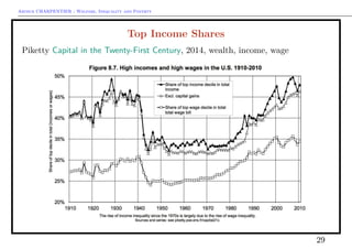
- 27. Arthur CHARPENTIER - Welfare, Inequality and Poverty Top Income Shares Piketty Capital in the Twenty-First Century, 2014 27
- 28. Arthur CHARPENTIER - Welfare, Inequality and Poverty Top Income Shares Piketty Capital in the Twenty-First Century, 2014 28
- 29. Arthur CHARPENTIER - Welfare, Inequality and Poverty Top Income Shares Piketty Capital in the Twenty-First Century, 2014, wealth, income, wage 29
- 30. Arthur CHARPENTIER - Welfare, Inequality and Poverty Top Income Shares Piketty Capital in the Twenty-First Century, 2014 30
- 31. Arthur CHARPENTIER - Welfare, Inequality and Poverty Fundamental Force of Divergence, r > g Piketty Capital in the Twenty-First Century, 2014 31
- 32. Arthur CHARPENTIER - Welfare, Inequality and Poverty Poverty, in France See Guélaud, Le nombre de pauvres a augmenté de 440.000 en France en 2010, 2012 La dernière enquête de l’Insee sur les niveaux de vie, rendue publique vendredi 7 septembre, est explosive. Que constate-t-elle en effet ? Qu’en 2010, le niveau de vie médian (19 270 euros annuels) a diminué de 0,5% par rapport à 2009, que seuls les plus riches s’en sont sortis et que la pauvreté, en hausse, frappe désormais 8,6 millions de personnes, soit 440 000 de plus qu’un an plus tôt. Avec la fin du plan de relance, les effets de la crise se sont fait sentir massivement. En 2009, la récession n’avait que ralenti la progression en euros constants du niveau de vie médian (+ 0,4%, contre + 1,7% par an en moyenne de 2004 à 2008). Il faut remonter à 2004, précise l’Insee, pour trouver un recul semblable à celui de 2010 (0,5%). 32
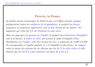
- 33. Arthur CHARPENTIER - Welfare, Inequality and Poverty Poverty, in France La timide reprise économique de 2010 n’a pas eu d’effets miracle, puisque pratiquement toutes les catégories de la population, y compris les classes moyennes ou moyennes supérieures, ont vu leur niveau de vie baisser. N’a augmenté que celui des 5% des Français les plus aisés. Dans un pays qui a la passion de l’égalité, la plupart des indicateurs d’inégalités sont à la hausse. L’indice de Gini, qui mesure le degré d’inégalité d’une distribution (en l’espèce, celle des niveaux de vie), a augmenté de 0,290 à 0,299 (0 correspondant à l’égalité parfaite et 1 à l’inégalité la plus forte). Le rapport entre la masse des niveaux de vie détenue par les 20 % les plus riches et celle détenue par les 20 % les plus modestes est passé de 4,3 à 4,5. 33
- 34. Arthur CHARPENTIER - Welfare, Inequality and Poverty Poverty, in France Déjà en hausse de 0,5 point en 2009, le taux de pauvreté monétaire a augmenté en 2010 de 0,6 point pour atteindre 14,1%, soit son plus haut niveau depuis 1997. 8,6 millions de personnes vivaient en 2010 en-dessous du seuil de pauvreté monétaire (964 euros par mois). Elles n’étaient que 8,1 millions en 2009. Mais il y a pire : une personne pauvre sur deux vit avec moins de 781 euros par mois En 2010, le chômage a peu contribuéà l’augmentation de la pauvreté (les chômeurs représentent à peine 4% de l’accroissement du nombre des personnes pauvres). C’est du coté des inactifs qu’il faut plutôt se tourner : les retraités (11%), les adultes inactifs autres que les étudiants et les retraites (16%) - souvent les titulaires de minima sociaux - et les enfants. Les moins de 18 ans contribuent pour près des deux tiers (63%) à l’augmentation du nombre de personnes pauvres [...] 34
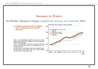
- 35. Arthur CHARPENTIER - Welfare, Inequality and Poverty Incomes in France See Houdré, Missègue & Seguin Inégalités de niveau de vie et pauvreté, 2012 35
- 36. Arthur CHARPENTIER - Welfare, Inequality and Poverty Incomes in France See Houdré, Missègue & Seguin Inégalités de niveau de vie et pauvreté, 2012 36
- 37. Arthur CHARPENTIER - Welfare, Inequality and Poverty Incomes in France See Houdré, Missègue & Seguin Inégalités de niveau de vie et pauvreté, 2012 37
- 38. Arthur CHARPENTIER - Welfare, Inequality and Poverty Incomes in France See Houdré, Missègue & Seguin Inégalités de niveau de vie et pauvreté, 2012 38
- 39. Arthur CHARPENTIER - Welfare, Inequality and Poverty Incomes in France See Houdré, Missègue & Seguin Inégalités de niveau de vie et pauvreté, 2012 39
- 40. Arthur CHARPENTIER - Welfare, Inequality and Poverty Incomes in France See Houdré, Missègue & Seguin Inégalités de niveau de vie et pauvreté, 2012 40
- 41. Arthur CHARPENTIER - Welfare, Inequality and Poverty Income ? See Statistics Canada Total Income, via Flachaire (2015). 41
- 42. Arthur CHARPENTIER - Welfare, Inequality and Poverty Income ? Micro vs macro Piketty Capital in the Twenty-First Century, 2014, 42
- 43. Arthur CHARPENTIER - Welfare, Inequality and Poverty Income ? Micro vs macro Piketty Capital in the Twenty-First Century, 2014, 43
- 44. Arthur CHARPENTIER - Welfare, Inequality and Poverty Income ? Micro vs macro To compare various household incomes • Oxford scale (OECD equivalent scale) ◦ 1.0 to the first adult ◦ 0.7 to each additional adult (aged 14, and more) ◦ 0.5 to each child • OECD-modified equivalent scale (late 90s by eurostat) ◦ 1.0 to the first adult ◦ 0.5 to each additional adult (aged 14, and more) ◦ 0.3 to each child • More recent OECD scale ◦ square root of household size 44
- 45. Arthur CHARPENTIER - Welfare, Inequality and Poverty Income ? Micro vs macro 45
- 46. Arthur CHARPENTIER - Welfare, Inequality and Poverty Income ? Tax Issues E.g. total taxes paid by total wage 46
- 47. Arthur CHARPENTIER - Welfare, Inequality and Poverty Income ? Tax Issues via Landais, Piketty & Saez Pour une révolution fiscale, 2011 47
- 48. Arthur CHARPENTIER - Welfare, Inequality and Poverty Income ? Tax Issues via Landais, Piketty & Saez Pour une révolution fiscale, 2011 48
- 49. Arthur CHARPENTIER - Welfare, Inequality and Poverty International Comparisons, Puchasing Power Parity See The Economist The Big Mac index, 2014 49
- 50. Arthur CHARPENTIER - Welfare, Inequality and Poverty International Comparisons, Puchasing Power Parity See The Economist The Big Mac index, 2014, via Flachaire 50
- 51. Arthur CHARPENTIER - Welfare, Inequality and Poverty International Comparisons, Puchasing Power Parity Piketty Capital in the Twenty-First Century, 2014, wealth, income, wage 51
- 52. Arthur CHARPENTIER - Welfare, Inequality and Poverty From Income and Wealth to Human Development The Human Development Index (HDI, see wikipedia) is a composite statistic of life expectancy, education, and income indices used to rank countries into four tiers of human development. It was created by Indian economist Amartya Sen and Pakistani economist Mahbub ul Haq in 1990, and was published by the United Nations Development Programme. The HDI is a composite index at value between 0 (awful) and 1 (perfect) based on the mixing of three basic indices aiming at representing on an equal footing measures of helth, education and standard of living. 52
- 53. Arthur CHARPENTIER - Welfare, Inequality and Poverty HDI Computation, new method (2010) Published on 4 November 2010 (and updated on 10 June 2011), starting with the 2010 Human Development Report the HDI combines three dimensions : — A long and healthy life : Life expectancy at birth — An education index : Mean years of schooling and Expected years of schooling — A decent standard of living : GNI per capita (PPP US$) In its 2010 Human Development Report, the UNDP began using a new method of calculating the HDI. The following three indices are used. The idea is to define a x index as x index = x − min (x) max (x) − min (x) 1. Health, Life Expectancy Index (LEI) = LE − 20 85 − 20 where LE is Life Expectancy at birth 53
- 54. Arthur CHARPENTIER - Welfare, Inequality and Poverty HDI Computation, new method (2010) 2. Education, Education Index (EI) = MYSI + EYSI 2 2.1 Mean Years of Schooling Index (MYSI) = MYS 15 where MYS is the Mean years of schooling (Years that a 25-year-old person or older has spent in schools) 2.2 Expected Years of Schooling Index (EYSI) = EYS 18 EYS : Expected years of schooling (Years that a 5-year-old child will spend with his education in his whole life) 3. Standard of Living Income Index (II) = log(GNIpc) − log(100) log(75, 000) − log(100) where GNIpc : Gross national income at purchasing power parity per capita Finally, the HDI is the geometric mean of the previous three normalized indices : HDI = 3 √ LEI · EI · II. 54
- 55. Arthur CHARPENTIER - Welfare, Inequality and Poverty Economic Well-Being See Osberg The Measurement of Economic Well-Being, 1985 and Osberg & Sharpe New Estimates of the Index of Economic Well-being, 2002 See also Jank & Owens Inequality in the United States, 2013, for stats and graphs about inequalities in the U.S., in terms of health, education, crime, etc. 55
- 56. Arthur CHARPENTIER - Welfare, Inequality and Poverty Various Aspects of Inequalities in the U.S. Jank & Owens Inequality in the United States, 2013 56
- 57. Arthur CHARPENTIER - Welfare, Inequality and Poverty Various Aspects of Inequalities in the U.S. Jank & Owens Inequality in the United States, 2013 57
- 58. Arthur CHARPENTIER - Welfare, Inequality and Poverty Various Aspects of Inequalities in the U.S. Jank & Owens Inequality in the United States, 2013 58
- 59. Arthur CHARPENTIER - Welfare, Inequality and Poverty Various Aspects of Inequalities in the U.S. Jank & Owens Inequality in the United States, 2013 59
- 60. Arthur CHARPENTIER - Welfare, Inequality and Poverty Various Aspects of Inequalities in the U.S. Jank & Owens Inequality in the United States, 2013 60
- 61. Arthur CHARPENTIER - Welfare, Inequality and Poverty Various Aspects of Inequalities in the U.S. Jank & Owens Inequality in the United States, 2013 61
- 62. Arthur CHARPENTIER - Welfare, Inequality and Poverty Various Aspects of Inequalities in the U.S. Jank & Owens Inequality in the United States, 2013 62
- 63. Arthur CHARPENTIER - Welfare, Inequality and Poverty Various Aspects of Inequalities in the U.S. Jank & Owens Inequality in the United States, 2013 63
- 64. Arthur CHARPENTIER - Welfare, Inequality and Poverty Various Aspects of Inequalities in the U.S. Jank & Owens Inequality in the United States, 2013 64
- 65. Arthur CHARPENTIER - Welfare, Inequality and Poverty Various Aspects of Inequalities in the U.S. Jank & Owens Inequality in the United States, 2013 65
- 66. Arthur CHARPENTIER - Welfare, Inequality and Poverty Various Aspects of Inequalities in the U.S. Jank & Owens Inequality in the United States, 2013 66
- 67. Arthur CHARPENTIER - Welfare, Inequality and Poverty Various Aspects of Inequalities in the U.S. Jank & Owens Inequality in the United States, 2013 67
- 68. Arthur CHARPENTIER - Welfare, Inequality and Poverty Various Aspects of Inequalities in the U.S. Jank & Owens Inequality in the United States, 2013 68
- 69. Arthur CHARPENTIER - Welfare, Inequality and Poverty Various Aspects of Inequalities in the U.S. Jank & Owens Inequality in the United States, 2013 69
- 70. Arthur CHARPENTIER - Welfare, Inequality and Poverty Various Aspects of Inequalities in the U.S. Jank & Owens Inequality in the United States, 2013 70
- 71. Arthur CHARPENTIER - Welfare, Inequality and Poverty Modeling Income Distribution Let {x1, · · · , xn} denote some sample. Then x = 1 n n i=1 xi = n i=1 1 n xi This can be used when we have census data. 1 load ( u r l ( " http : // freakonometrics . f r e e . f r / income_5. RData" ) ) 2 income <− s o r t ( income ) 3 plot ( 1 : 5 , income ) income qq q q q 0 50000 100000 150000 200000 250000 It is possible to use survey data. If πi denote the probability to be drawn, use weights ωi ∝ 1 nπi 71
- 72. Arthur CHARPENTIER - Welfare, Inequality and Poverty The weighted average is then xω = n i=1 ωi ω xi where ω = ωi. This is an unbaised estimator of the population mean. Sometime, data are obtained from stratified samples : before sampling, members of the population are groupes in homogeneous subgroupes (called a strata). Given S strata, such that the population in strata s is Ns, then xS = S s=1 Ns N xs where xs = 1 Ns i∈Ss xi 72
- 73. Arthur CHARPENTIER - Welfare, Inequality and Poverty Statistical Tools Used to Describe the Distribution Consider a sample {x1, · · · , xn}. Usually, the order is not important. So let us order those values, x1:n min{xi} ≤ x2:n ≤ · · · ≤ xn−1:n ≤ xn:n max{xi} As usual, assume that xi’s were randomly drawn from an (unknown) distribution F. If F denotes the cumulative distribution function, F(x) = P(X ≤ x), one can prove that F(xi:n) = P(X ≤ xi:n) ∼ i n The quantile function is defined as the inverse of the cumulative distribution function F, Q(u) = F−1 (u) or F(Q(u)) = P(X ≤ Q(u)) = u 73
- 74. Arthur CHARPENTIER - Welfare, Inequality and Poverty Lorenz curve The empirical version of Lorenz curve is L = i n , 1 nx j≤i xj:n 1 > plot ( ( 0 : 5 ) / 5 , c (0 ,cumsum( income ) /sum( income ) ) ) 74 0.0 0.2 0.4 0.6 0.8 1.0 0.0 0.2 0.4 0.6 0.8 1.0 Lorenz curve p L(p) q q q q
- 75. Arthur CHARPENTIER - Welfare, Inequality and Poverty Gini Coefficient Gini coefficient is defined as the ratio of areas, A A + B . It can be defined using order statistics as G = 2 n(n − 1)x n i=1 i · xi:n − n + 1 n − 1 1 > n <− length ( income ) 2 > mu <− mean( income ) 3 > 2∗sum ( ( 1 : n) ∗ s o r t ( income ) ) / (mu∗n∗ (n−1))−(n +1)/ (n−1) 4 [ 1 ] 0.5800019 75 q q 0.0 0.2 0.4 0.6 0.8 1.0 0.00.20.40.60.81.0 p L(p) q q q qA B
- 76. Arthur CHARPENTIER - Welfare, Inequality and Poverty Distribution Fitting Assume that we now have more observations, 1 > load ( u r l ( " http : // freakonometrics . f r e e . f r /income_500. RData" ) ) We can use some histogram to visualize the distribu- tion of the income 1 > summary( income ) 2 Min . 1 st Qu. Median Mean 3rd Qu. Max. 3 2191 23830 42750 77010 87430 2003000 4 > s o r t ( income ) [ 4 9 5 : 5 0 0 ] 5 [ 1 ] 465354 489734 512231 539103 627292 2003241 6 > h i s t ( income , breaks=seq (0 ,2005000 , by=5000) ) Histogram of income income Frequency 0 500000 1000000 1500000 2000000 010203040 76
- 77. Arthur CHARPENTIER - Welfare, Inequality and Poverty Distribution Fitting Because of the dispersion, look at the histogram of the logarithm of the data 1 > h i s t ( log ( income , 1 0 ) , breaks=seq ( 3 , 6 . 5 , length =51) ) 2 > boxplot ( income , h o r i z o n t a l=TRUE, log=" x " ) qqqqqqqqqqqqqqqqqqqqqqqqqqqqqqqqqqqqqqqqqqqqq q q 2e+03 1e+04 5e+04 2e+05 1e+06 Histogram of log(income, 10) log(income, 10) Frequency 3.0 3.5 4.0 4.5 5.0 5.5 6.0 6.5 010203040 77
- 78. Arthur CHARPENTIER - Welfare, Inequality and Poverty Distribution Fitting The cumulative distribution function (on the log of the income) 1 > u <− s o r t ( income ) 2 > v <− ( 1 : 5 0 0 ) /500 3 > plot (u , v , type=" s " , log=" x " ) Income (log scale) CumulatedProbabilities 2e+03 1e+04 5e+04 2e+05 1e+06 0.00.20.40.60.81.0 78
- 79. Arthur CHARPENTIER - Welfare, Inequality and Poverty Distribution Fitting If we invert that graph, we have the quantile function 1 > plot (v , u , type=" s " , c o l=" red " , log=" y " ) 79 Probabilities Income(logscale) 0.0 0.2 0.4 0.6 0.8 1.0 2e+031e+045e+042e+051e+06
- 80. Arthur CHARPENTIER - Welfare, Inequality and Poverty Distribution Fitting On that dataset, Lorenz curve is 1 > plot ( ( 0 : 5 0 0 ) / 500 , c (0 ,cumsum( income ) /sum( income ) ) ) q q 0.0 0.2 0.4 0.6 0.8 1.0 0.00.20.40.60.81.0 p L(p) 80
- 81. Arthur CHARPENTIER - Welfare, Inequality and Poverty Distribution and Confidence Intervals There are two techniques to get the distribution of an estimator θ, — a parametric one, based on some assumptions on the underlying distribution, — a nonparametric one, based on sampling techniques If Xi’s have a N(µ, σ2 ) distribution, then X ∼ N µ, σ2 n But sometimes, distribution can only be obtained as an approximation, because of asymptotic properties. From the central limit theorem, X → N µ, σ2 n as n → ∞. In the nonparametric case, the idea is to generate pseudo-samples of size n, by resampling from the original distribution. 81
- 82. Arthur CHARPENTIER - Welfare, Inequality and Poverty Bootstraping Consider a sample x = {x1, · · · , xn}. At step b = 1, 2, · · · , B, generate a pseudo sample xb by sampling (with replacement) within sample x. Then compute any statistic θ(xb ) 1 > boot <− function ( sample , f , b=500){ 2 + F <− rep (NA, b) 3 + n <− length ( sample ) 4 + f o r ( i in 1: b) { 5 + idx <− sample ( 1 : n , s i z e=n , r e p l a c e=TRUE) 6 + F[ i ] <− f ( sample [ idx ] ) } 7 + return (F) } 82
- 83. Arthur CHARPENTIER - Welfare, Inequality and Poverty Bootstraping Let us generate 10,000 bootstraped sample, and com- pute Gini index on those 1 >boot_g i n i <− boot ( income , gini ,1 e4 ) To visualize the distribution of the index 1 > h i s t ( boot_gini , p r o b a b i l i t y=TRUE) 2 > u <− seq ( . 4 , . 7 , length =251) 3 > v <− dnorm(u , mean( boot_g i n i ) , sd ( boot_g i n i ) ) 4 > l i n e s (u , v , c o l=" red " , l t y =2) boot_gini Density 0.45 0.50 0.55 0.60 051015 83
- 84. Arthur CHARPENTIER - Welfare, Inequality and Poverty Continuous Versions The empirical cumulative distribution function Fn(x) = 1 n n i=1 1(xi ≤ x) Observe that Fn(xj:n) = j n If F is absolutely continuous, F(x) = x 0 f(t)dt i.e. f(x) = dF(x) dx . Then P(x ∈ [a, b]) = b a f(t)dt = F(b) − F(a). 84
- 85. Arthur CHARPENTIER - Welfare, Inequality and Poverty Continuous Versions One can define quantiles as x = Q(p) = F−1 (p) The expected value is µ = ∞ 0 xf(x)dx = ∞ 0 [1 − F(x)]dx = 1 0 Q(p)dp. We can compute the average standard of living of the group below z. This is equivalent to the expectation of a truncated distribution. µ− z = 1 F(z) z 0 xf(x)dx = ∞ 0 1 − F(x) F(z) fx 85
- 86. Arthur CHARPENTIER - Welfare, Inequality and Poverty Continuous Versions Lorenz curve is p → L(p) with L(p) = 1 µ Q(p) 0 xf(x)dx Gastwirth (1971) proved that L(p) = 1 µ p 0 Q(u)du = p 0 Q(u)du 1 0 Q(u)du The numerator sums the incomes of the bottom p proportion of the population. The denominator sums the incomes of all the population. L is a [0, 1] → [0, 1] function, continuous if F is continuous. Observe that L is increasing, since dL(p) dp = Q(p) µ Further, L is convex 86
- 87. Arthur CHARPENTIER - Welfare, Inequality and Poverty The sample case L i n = i j=1 xj:n n j=1 xj:n The points {i/n, L(i/n)} are then linearly interpolated to complete the corresponding Lorenz curve. The continuous distribution case L(p) = F −1 (p) 0 ydF(y) ∞ 0 ydF(y) = 1 E(X) p 0 F−1 (u)du with p ∈ (0, 1). Let L be a continuous function on [0, 1], then L is a Lorenz curve if and only if L(0) = 0, L(1) = 1, L (0+ ) ≥ 0 and L (p) ≥ 0 on [0, 1]. 87
- 88. Arthur CHARPENTIER - Welfare, Inequality and Poverty From Lorenz to Bonferroni The Bonferroni curve is B(p) = L(p) p and the Bonferroni index is BI = 1 − 1 0 B(p)dp. Define Pi = i n and Qi = 1 nx i j=1 xj then B = 1 n − 1 n−1 i=1 Pi − Qi Pi 88
- 89. Arthur CHARPENTIER - Welfare, Inequality and Poverty Gini and Pietra indices The Gini index is defined as twice the area between the egalitarian line and the Lorenz curve G = 2 1 0 [p − L(p)]dp = 1 − 2 1 0 L(p)dp which can also be writen 1 − 1 E(X) ∞ 0 [1 − F(x)]2 dx Pietra index is defined as the maximal vertical deviation between the Lorenz curve and the egalitarian line P = max p∈(0,1) {p − L(p)} = E(|X − E(X)|) 2E(X) if F is strictly increasing (the maximum is reached in p = F(E(X))) 89
- 90. Arthur CHARPENTIER - Welfare, Inequality and Poverty Examples E.g. consider the uniform distribution F(x) = min{1, x − a b − a 1(x ≥ a)} Then L(p) = 2ap + (b − a)2 p2 a + b and Gini index is G = b − a 3(a + b) E.g. consider a Pareto distribution, F(x) = 1 − x0 x α , x ≥ x0, with shape parameter α > 0. Then F−1 (u) = x0 (1 − u) 1 α 90
- 91. Arthur CHARPENTIER - Welfare, Inequality and Poverty and L(p) = 1 − [1 − p]1− 1 α p ∈ (0, 1). and Gini index is G = 1 2α − 1 while Pietra index is, if α > 1 P = (α − 1)α−1 αα E.g. consider the lognormal distribution, F(x) = Φ log x − µ σ then L(p) = Φ(Φ−1 (p) − σ) p ∈ (0, 1). and Gini index is G = 2Φ σ √ 2 − 1 91
- 92. Arthur CHARPENTIER - Welfare, Inequality and Poverty Fitting a Distribution The standard technique is based on maximum likelihood estimation, provided by 1 > l i b r a r y (MASS) 2 > f i t d i s t r ( income , " lognormal " ) 3 meanlog sdlog 4 10.72264538 1.01091329 5 ( 0.04520942) ( 0.03196789) For other distribution (such as the Gamma distribution), we might have to rescale 1 > ( f i t_g <− f i t d i s t r ( income/1e2 , "gamma" ) ) 2 shape rate 3 1.0812757769 0.0014040438 4 (0.0473722529) (0.0000544185) 5 > ( f i t_ln <− f i t d i s t r ( income/1e2 , " lognormal " ) ) 6 meanlog sdlog 7 6.11747519 1.01091329 8 (0.04520942) (0.03196789) 92
- 93. Arthur CHARPENTIER - Welfare, Inequality and Poverty Fitting a Distribution We can compare the densities 1 > u=seq (0 ,2 e5 , length =251) 2 > h i s t ( income , breaks=seq (0 ,2005000 , by=5000) , c o l=rgb ( 0 , 0 , 1 , . 5 ) , border=" white " , xlim=c (0 ,2 e5 ) , p r o b a b i l i t y=TRUE) 3 > v_g <− dgamma(u/1e2 , f i t_g$ estimate [ 1 ] , f i t _g$ estimate [ 2 ] ) /1e2 4 > v_ln <− dlnorm (u/1e2 , f i t_ln $ estimate [ 1 ] , f i t_ln $ estimate [ 2 ] ) /1e2 5 > l i n e s (u , v_g , c o l=" red " , l t y =2) 6 > l i n e s (u , v_ln , c o l=rgb ( 1 , 0 , 0 , . 4 ) ) Income CumulatedProbabilities 0 50000 100000 150000 200000 0.00.20.40.60.81.0 Gamma Log Normal 93
- 94. Arthur CHARPENTIER - Welfare, Inequality and Poverty Fitting a Distribution or the cumuluative distributions 1 x <− s o r t ( income ) 2 y <− ( 1 : 5 0 0 ) /500 3 plot (x , y , type=" s " , c o l=" black " ) 4 v_g <− pgamma(u/1e2 , f i t_g$ estimate [ 1 ] , f i t_g $ estimate [ 2 ] ) 5 v_ln <− plnorm (u/1e2 , f i t_ln $ estimate [ 1 ] , f i t _ln $ estimate [ 2 ] ) 6 l i n e s (u , v_g , c o l=" red " , l t y =2) 7 l i n e s (u , v_ln , c o l=rgb ( 1 , 0 , 0 , . 4 ) ) income Density 0 50000 100000 150000 200000 0.0e+005.0e−061.0e−051.5e−05 Gamma Log Normal One might consider the parametric version of Lorenz curve, to confirm the goodness of fit, e.g. a lognormal distribution with σ = 1 since 1 > f i t d i s t r ( income , " lognormal " ) 2 meanlog sdlog 3 10.72264538 1.01091329 94
- 95. Arthur CHARPENTIER - Welfare, Inequality and Poverty Fitting a Distribution We can use functions of R 1 l i b r a r y ( ineq ) 2 Lc . sim <− Lc ( income ) 3 plot ( 0 : 1 , 0 : 1 , xlab="p" , ylab="L(p) " , c o l=" white " ) 4 polygon ( c (0 ,1 ,1 ,0) , c (0 ,0 ,1 ,0) , c o l=rgb ( 0 , 0 , 1 , . 1 ) , border=NA) 5 polygon ( Lc . sim$p , Lc . sim$L , c o l=rgb ( 0 , 0 , 1 , . 3 ) , border=NA) 6 l i n e s ( Lc . sim ) 7 segments (0 ,0 ,1 ,1) 8 l i n e s ( Lc . lognorm , parameter =1, l t y =2) q q 0.0 0.2 0.4 0.6 0.8 1.0 0.00.20.40.60.81.0 p L(p) 95
- 96. Arthur CHARPENTIER - Welfare, Inequality and Poverty Standard Parametric Distribution For those distributions, we mention the R names in the gamlss package. Inference can be done using 1 f i t <−gamlss (y~ 1 , family=LNO) • log normal f(x) = 1 xσ √ 2π e− (ln x−µ)2 2σ2 , x ≥ 0 with mean eµ+σ2 /2 , median eµ , and variance (eσ2 − 1)e2µ+σ2 1 LNO(mu. l i n k = " i d e n t i t y " , sigma . l i n k = " log " ) 2 dLNO(x , mu = 1 , sigma = 0.1 , nu = 0 , log = FALSE) • gamma f(x) = x1/σ2 −1 exp[−x/(σ2 µ)] (σ2µ)1/σ2 Γ(1/σ2) , x ≥ 0 96
- 97. Arthur CHARPENTIER - Welfare, Inequality and Poverty with mean µ and variance σ2 1 GA(mu. l i n k = " log " , sigma . l i n k =" log " ) 2 dGA(x , mu = 1 , sigma = 1 , log = FALSE) • Pareto f(x) = α xα m xα+1 for x ≥ xm with cumulated distribution F(x) = 1 − xm x α for x ≥ xm with mean αxm (α − 1) if α > 1, and variance x2 mα (α − 1)2(α − 2) if α > 2. 1 PARETO2(mu. l i n k = " log " , sigma . l i n k = " log " ) 2 dPARETO2(x , mu = 1 , sigma = 0.5 , log = FALSE) 97
- 98. Arthur CHARPENTIER - Welfare, Inequality and Poverty Larger Families • GB1 - generalized Beta type 1 f(x) = |a|xap−1 (1 − (x/b)a )q−1 bapB(p, q) , 0 < xa < ba where b , p , and q are positive 1 GB1(mu. l i n k = " l o g i t " , sigma . l i n k = " l o g i t " , nu . l i n k = " log " , tau . l i n k = " log " ) 2 dGB1(x , mu = 0.5 , sigma = 0.4 , nu = 1 , tau = 1 , log = FALSE) The GB1 family includes the generalized gamma(GG), and Pareto as special cases. • GB2 - generalized Beta type 2 f(x) = |a|xap−1 bapB(p, q)(1 + (x/b)a)p+q 98
- 99. Arthur CHARPENTIER - Welfare, Inequality and Poverty 1 GB2(mu. l i n k = " log " , sigma . l i n k = " i d e n t i t y " , nu . l i n k = " log " , tau . l i n k = " log " ) 4 dGB2(x , mu = 1 , sigma = 1 , nu = 1 , tau = 0 .5 , log = FALSE) The GB2 nests common distributions such as the generalized gamma (GG), Burr, lognormal, Weibull, Gamma, Rayleigh, Chi-square, Exponential, and the log-logistic. • Generalized Gamma f(x) = (p/ad )xd−1 e−(x/a)p Γ(d/p) , 99
- 100. Arthur CHARPENTIER - Welfare, Inequality and Poverty Dealing with Binned Data 1 > load ( u r l ( " http : // freakonometrics . f r e e . f r /income_binned . RData" ) ) 2 > head ( income_binned ) 3 low high number mean std_e r r 4 1 0 4999 95 3606 964 5 2 5000 9999 267 7686 1439 6 3 10000 14999 373 12505 1471 7 4 15000 19999 350 17408 1368 8 5 20000 24999 329 22558 1428 9 6 25000 29999 337 27584 1520 10 > t a i l ( income_binned ) 11 low high number mean std_e r r 12 46 225000 229999 10 228374 1197 13 47 230000 234999 13 232920 1370 14 48 235000 239999 11 236341 1157 15 49 240000 244999 14 242359 1474 16 50 245000 249999 11 247782 1487 17 51 250000 I n f 228 395459 189032 100
- 101. Arthur CHARPENTIER - Welfare, Inequality and Poverty Dealing with Binned Data There is a dedicated package to work with such datasets, 1 > l i b r a r y ( b i n e q u a l i t y ) To fit a parametric distribution, e.g. a log-normal distribution, use functions of R 1 > n <− nrow ( income_binned ) 2 > f i t_LN <− fitFunc (ID=rep ( " Fake Data " ,n) , hb=income_binned [ , " number " ] , bin_min=income_binned [ , " low " ] , bin_max=income_binned [ , " high " ] , obs_mean=income_binned [ , "mean" ] , ID_name=" Country " , d i s t r i b u t i o n= LNO, distName="LNO" ) 3 Time d i f f e r e n c e of 0.09900618 s e c s 4 f o r LNO f i t across 1 d i s t r i b u t i o n s 101
- 102. Arthur CHARPENTIER - Welfare, Inequality and Poverty Dealing with Binned Data To visualize the cumulated distribution function, use 1 > N <− income_binned $number 2 > y1 <− cumsum(N) /sum(N) 3 > u <− seq (min( income_binned $low ) ,max( income _binned $low ) , length =101) 4 > v <− plnorm (u , f i t_LN$ parameters [ 1 ] , f i t_LN$ parameters [ 2 ] ) 5 > plot (u , v , c o l=" blue " , type=" l " , lwd=2, xlab=" Income " , ylab=" Cumulative Probability " ) 6 > f o r ( i in 1 : ( n−1)) r e c t ( income_binned $low [ i ] , 0 , income_binned $ high [ i ] , y1 [ i ] , c o l=rgb ( 1 , 0 , 0 , . 2 ) ) 7 > f o r ( i in 1 : ( n−1)) r e c t ( income_binned $low [ i ] , y1 [ i ] , income_binned $ high [ i ] , c (0 , y1 ) [ i ] , c o l=rgb ( 1 , 0 , 0 , . 4 ) ) 0 50000 100000 150000 200000 250000 0.00.20.40.60.8 Income CumulativeProbability 102
- 103. Arthur CHARPENTIER - Welfare, Inequality and Poverty Dealing with Binned Data and to visualize the cumulated distribution function, use 1 > N=income_binned $number 2 > y2=N/sum(N) / d i f f ( income_binned $low ) 3 > u=seq (min( income_binned $low ) ,max( income_ binned $low ) , length =101) 4 > v=dlnorm (u , f i t_LN$ parameters [ 1 ] , f i t_LN$ parameters [ 2 ] ) 5 > plot (u , v , c o l=" blue " , type=" l " , lwd=2, xlab=" Income " , ylab=" Density " ) 6 > f o r ( i in 1 : ( n−1)) r e c t ( income_binned $low [ i ] , 0 , income_binned $ high [ i ] , y2 [ i ] , c o l=rgb ( 1 , 0 , 0 , . 2 ) , border=" white " ) 0 50000 100000 150000 200000 250000 0.0e+005.0e−061.0e−051.5e−05 Income Density 103
- 104. Arthur CHARPENTIER - Welfare, Inequality and Poverty Dealing with Binned Data But it is also possible to estimate all GB-distributions at once, 1 > f i t s=run_GB_family (ID=rep ( " Fake Data " ,n) ,hb=income_binned [ , " number " ] , bin_min=income_binned [ , " low " ] , bin_max=income_binned [ , " high " ] , obs _mean=income_binned [ , "mean" ] , 2 + ID_name=" Country " ) 3 Time d i f f e r e n c e of 0.03800201 s e c s 4 f o r GB2 f i t across 1 d i s t r i b u t i o n s 5 6 Time d i f f e r e n c e of 0.3090181 s e c s 7 f o r GG f i t across 1 d i s t r i b u t i o n s 8 9 Time d i f f e r e n c e of 0.864049 s e c s 10 f o r BETA2 f i t across 1 d i s t r i b u t i o n s ... 1 Time d i f f e r e n c e of 0.04900193 s e c s 104
- 105. Arthur CHARPENTIER - Welfare, Inequality and Poverty 2 f o r LOGLOG f i t across 1 d i s t r i b u t i o n s 3 6 Time d i f f e r e n c e of 1.865106 s e c s 7 f o r PARETO2 f i t across 1 d i s t r i b u t i o n s 1 > f i t s $ f i t . f i l t e r [ , c ( " g i n i " , " a i c " , " bic " ) ] 2 g i n i a i c bic 3 1 NA NA NA 4 2 5.054377 34344.87 34364.43 5 3 5.110104 34352.93 34372.48 6 4 NA 53638.39 53657.94 7 5 4.892090 34845.87 34865.43 8 6 5.087506 34343.08 34356.11 9 7 4.702194 34819.55 34832.59 10 8 4.557867 34766.38 34779.41 11 9 NA 58259.42 58272.45 12 10 5.244332 34805.70 34818.73 1 > f i t s $ best_model$ a i c 105
- 106. Arthur CHARPENTIER - Welfare, Inequality and Poverty 2 Country obsMean d i s t r i b u t i o n estMean var 5 1 Fake Data NA LNO 72328.86 6969188937 6 cv cv_sqr g i n i t h e i l MLD 7 1 1.154196 1.332168 5.087506 0.4638252 0.4851275 8 a i c bic didConverge l o gL ike li ho od nparams 9 1 34343.08 34356.11 TRUE −17169.54 2 10 median sd 11 1 44400.23 83481.67 That was easy, those were simulated data... 106
- 107. Arthur CHARPENTIER - Welfare, Inequality and Poverty Dealing with Binned Data Consider now some real data, 1 > data = read . table ( " http : // freakonometrics . f r e e . f r /us_income . txt " , sep=" , " , header=TRUE) 2 > head ( data ) 3 low high number_1000 s mean std_e r r 4 1 0 4999 4245 1249 50 5 2 5000 9999 5128 7923 30 6 3 10000 14999 7149 12389 28 7 4 15000 19999 7370 17278 26 8 > t a i l ( data ) 9 low high number_1000 s mean std_e r r 10 39 190000 194999 361 192031 115 11 40 195000 199999 291 197120 135 12 41 200000 249999 2160 219379 437 13 42 250000 9999999 2498 398233 6519 107
- 108. Arthur CHARPENTIER - Welfare, Inequality and Poverty Dealing with Binned Data To fit a parametric distribution, e.g. a log-normal distribution, use 1 > n <− nrow ( data ) 2 > f i t_LN <− fitFunc (ID=rep ( "US" ,n) , hb=data [ , " number_1000 s " ] , bin_min =data [ , " low " ] , bin_max=data [ , " high " ] , obs_mean=data [ , "mean" ] , ID_ name=" Country " , d i s t r i b u t i o n=LNO, distName="LNO" ) 3 Time d i f f e r e n c e of 0.1040058 s e c s 4 f o r LNO f i t across 1 d i s t r i b u t i o n s 108
- 109. Arthur CHARPENTIER - Welfare, Inequality and Poverty Dealing with Binned Data To visualize the cumulated distribution function, use 1 > N <− income_binned $number 2 > y1 <− cumsum(N) /sum(N) 3 > u <− seq (min( income_binned $low ) ,max( income _binned $low ) , length =101) 4 > v <− plnorm (u , f i t_LN$ parameters [ 1 ] , f i t_LN$ parameters [ 2 ] ) 5 > plot (u , v , c o l=" blue " , type=" l " , lwd=2, xlab=" Income " , ylab=" Cumulative Probability " ) 6 > f o r ( i in 1 : ( n−1)) r e c t ( income_binned $low [ i ] , 0 , income_binned $ high [ i ] , y1 [ i ] , c o l=rgb ( 1 , 0 , 0 , . 2 ) ) 7 > f o r ( i in 1 : ( n−1)) r e c t ( income_binned $low [ i ] , y1 [ i ] , income_binned $ high [ i ] , c (0 , y1 ) [ i ] , c o l=rgb ( 1 , 0 , 0 , . 4 ) ) 0 50000 100000 150000 200000 250000 0.00.20.40.60.8 Income CumulativeProbability 109
- 110. Arthur CHARPENTIER - Welfare, Inequality and Poverty Dealing with Binned Data and to visualize the cumulated distribution function, use 1 > N=income_binned $number 2 > y2=N/sum(N) / d i f f ( income_binned $low ) 3 > u=seq (min( income_binned $low ) ,max( income_ binned $low ) , length =101) 4 > v=dlnorm (u , f i t_LN$ parameters [ 1 ] , f i t_LN$ parameters [ 2 ] ) 5 > plot (u , v , c o l=" blue " , type=" l " , lwd=2, xlab=" Income " , ylab=" Density " ) 6 > f o r ( i in 1 : ( n−1)) r e c t ( income_binned $low [ i ] , 0 , income_binned $ high [ i ] , y2 [ i ] , c o l=rgb ( 1 , 0 , 0 , . 2 ) , border=" white " ) 0 50000 100000 150000 200000 250000 0.0e+005.0e−061.0e−051.5e−05 Income Density 110
- 111. Arthur CHARPENTIER - Welfare, Inequality and Poverty Dealing with Binned Data And the winner is.... 1 > f i t s $ f i t . f i l t e r [ , c ( " g i n i " , " a i c " , " bic " ) ] 2 g i n i a i c bic 3 1 4.413411 825368.7 825407.4 4 2 4.395078 825598.8 825627.9 5 3 4.455112 825502.4 825531.5 6 4 4.480844 825881.5 825910.6 7 5 4.413282 825315.3 825344.4 8 6 4.922123 832408.2 832427.6 9 7 4.341085 827065.2 827084.6 10 8 4.318694 826112.9 826132.2 11 9 NA 831054.2 831073.6 12 10 NA NA NA 1 > f i t s $ best_model$ a i c 2 Country obsMean d i s t r i b u t i o n estMean var 3 1 US NA GG 65147.54 3152161910 111
- 112. Arthur CHARPENTIER - Welfare, Inequality and Poverty 4 cv cv_sqr g i n i t h e i l MLD 7 1 0.8617995 0.7426984 4.395078 0.3251443 0.3904942 8 a i c bic didConverge l o gL ike li ho od nparams 9 1 825598.8 825627.9 TRUE −412796.4 3 10 median sd 11 1 48953.6 56144.12 112
- 113. Arthur CHARPENTIER - Welfare, Inequality and Poverty Inequality Comparisons (2-person Economy) not much to say... any measure of dispersion is appropriate — income gap x2 − x1 — proportional gap x2 x1 — any functional of the distance |x2 − x1| graphs are from Amiel & Cowell (1999, ebooks.cambridge.org ) 113
- 114. Arthur CHARPENTIER - Welfare, Inequality and Poverty Inequality Comparisons (3-person Economy) Consider any 3-person economy, with incomes x = {x1, x2, x3}. This point can be visualized in Kolm triangle. 114
- 115. Arthur CHARPENTIER - Welfare, Inequality and Poverty Inequality Comparisons (3-person Economy) 1 kolm=function (p=c (200 ,300 ,500) ) { 2 p1=p/sum(p) 3 y0=p1 [ 2 ] 4 x0=(2∗p1 [1]+ y0 ) / sqrt (3) 5 plot ( 0 : 1 , 0 : 1 , c o l=" white " , xlab=" " , ylab=" " , 6 axes=FALSE, ylim=c (0 ,1) ) 7 polygon ( c ( 0 , . 5 , 1 , 0 ) , c ( 0 , . 5 ∗ sqrt (3) ,0 ,0) ) 8 points ( x0 , y0 , pch=19, c o l=" red " ) } 115
- 116. Arthur CHARPENTIER - Welfare, Inequality and Poverty Inequality Comparisons (n-person Economy) In a n-person economy, comparison are clearly more difficult 116
- 117. Arthur CHARPENTIER - Welfare, Inequality and Poverty Inequality Comparisons (n-person Economy) Why not look at inequality per subgroups, If we focus at the top of the distribution (same holds for the bottom), → rising inequality If we focus at the middle of the distri- bution, → falling inequality 117
- 118. Arthur CHARPENTIER - Welfare, Inequality and Poverty Inequality Comparisons (n-person Economy) To measure inequality, we usually — define ‘equality’ based on some reference point / distribution — define a distance to the reference point / distribution — aggregate individual distances We want to visualize the distribution of incomes 1 > income <− read . csv ( " http : //www. vchar ite . univ−mrs . f r /pp/ lubrano / cours / f e s 9 6 . csv " , sep=" ; " , header=FALSE) $V1 F(x) = P(X ≤ x) = x 0 f(t)dt 118
- 119. Arthur CHARPENTIER - Welfare, Inequality and Poverty Densities are usually difficult to com- pare, 1 > h i s t ( income , 2 + breaks=seq (min( income ) −1,max( income ) +50,by=50) , 3 + p r o b a b i l i t y=TRUE) 4 > l i n e s ( density ( income ) , c o l=" red " , lwd=2) Histogram of income income Density 0 500 1000 1500 2000 2500 3000 0.0000.0010.0020.0030.004 119
- 120. Arthur CHARPENTIER - Welfare, Inequality and Poverty It is more convenient, compare cumu- lative distribution functions of income, wealth, consumption, grades, etc. 1 > plot ( ecdf ( income ) ) 0 1000 2000 3000 0.00.20.40.60.81.0 ecdf(income) x Fn(x) 120
- 121. Arthur CHARPENTIER - Welfare, Inequality and Poverty The Parade of Dwarfs An alternative is to use Pen’s parade, also called the parade of dwarfs (and a few giants), “parade van dwergen en een enkele reus”. The height of each person is stretched in the proportion to his or her income everyone is line up in order of height, shortest (poorest) are on the left and tallest (richest) are on the right let them walk some time, like a procession. 121
- 122. Arthur CHARPENTIER - Welfare, Inequality and Poverty c.d.f., quantiles and Lorenz 1 > Pen( income ) 0.0 0.2 0.4 0.6 0.8 1.0 0 2 4 6 8 10 Pen's Parade i n x(i)x 122
- 123. Arthur CHARPENTIER - Welfare, Inequality and Poverty c.d.f., quantiles and Lorenz This parade of the Dwarfs function is just the quantile function. 1 > q <− function (u) qua nti le ( income , u) see also 1 > n <− length ( income ) 2 > u <− seq (1 / (2 ∗n) ,1−1/ (2 ∗n) , length=n) 3 > plot (u , s o r t ( income ) , type=" l " ) plot ( ecdf ( income ) ) 0.0 0.2 0.4 0.6 0.8 1.0 050010001500200025003000 u sort(income) 123
- 124. Arthur CHARPENTIER - Welfare, Inequality and Poverty c.d.f., quantiles and Lorenz To get Lorentz curve, we substitute on the y-axis proportion of incomes to incomes. 1 > l i b r a r y ( ineq ) 2 > Lc ( income ) 3 > L <− function (u) Lc ( income ) $L [ round (u∗ length ( income ) ) ] 0.0 0.2 0.4 0.6 0.8 1.0 0.0 0.2 0.4 0.6 0.8 1.0 Lorenz curve p L(p) 124
- 125. Arthur CHARPENTIER - Welfare, Inequality and Poverty c.d.f., quantiles and Lorenz x-axis y-axis c.d.f. income proportion of population Pen’s parade (quantile) proportion of population income Lorenz curve proportion of population proportion of income 125
- 126. Arthur CHARPENTIER - Welfare, Inequality and Poverty Standard statistical measure of dispersion The variance for a sample X = {x1, · · · , xn} is Var(X) = 1 n n i=1 [xi − x]2 where the baseline (reference) is x = 1 n n i=1 xi. 1 > var ( income ) 2 [ 1 ] 34178.43 problem it is a quadratic function, Var(αX) = α2 Var(X). 126
- 127. Arthur CHARPENTIER - Welfare, Inequality and Poverty Standard statistical measure of dispersion An alternative is the coefficient of variation, cv(X) = Var(X) x But not a good measure to capture inequality overall, very sensitive to very high incomes 1 > cv <− function ( x) sd (x ) /mean( x) 2 > cv ( income ) 3 [ 1 ] 0.6154011 127
- 128. Arthur CHARPENTIER - Welfare, Inequality and Poverty Standard statistical measure of dispersion An alternative is to use a logarithmic transformation. Use the logarithmic variance Varlog(X) = 1 n n i=1 [log(xi) − log(x)]2 1 > var_log <− function ( x ) var ( log (x ) ) 2 > var_log ( income ) 3 [ 1 ] 0.2921022 Those measures are distances on the x-axis. 128
- 129. Arthur CHARPENTIER - Welfare, Inequality and Poverty Standard statistical measure of dispersion Other inequality measures can be derived from Pen’s parade of the Dwarfs, where measures are based on distances on the y-axis, i.e. distances between quantiles. Qp = F−1 (p) i.e. F(Qp) = p e.g. the median is the quantile when p = 50%, the first quartile is the quantile when p = 25%, the first quintile is the quantile when p = 20%, the first decile is the quantile when p = 10%, the first percentile is the quantile when p = 1% 1 > qua n t ile ( income , c ( . 1 , . 5 , . 9 , . 9 9 ) ) 2 10% 50% 90% 99% 3 137.6294 253.9090 519.6887 933.9211 129
- 130. Arthur CHARPENTIER - Welfare, Inequality and Poverty Standard statistical measure of dispersion Define the quantile ratio as Rp = Q1−p Qp In case of perfect equality, Rp = 1. The most popular one is probably the 90/10 ratio. 1 > R_p <− function (x , p) q uant ile (x ,1−p) / q uantil e (x , p) 2 > R_p( income , . 1 ) 3 90% 4 3.776 0.0 0.2 0.4 0.6 0.8 1.0 051015 probability R This index measures the gap between the rich and the poor. 130
- 131. Arthur CHARPENTIER - Welfare, Inequality and Poverty E.g. R0.1 = 10 means that top 10% incomes are more than 10 times higher than the bottom 10% incomes. Ignores the distribution (apart from the two points), violates transfer principle. An alternative measure might be Kuznets Ratio, defined from Lorenz curve as the ratio of the share of income earned by the poorest p share of the population and the richest r share of the population, I(p, r) = L(p) 1 − L(1 − r) But here again, it ignores the distribution between the cutoffs and therefore violates the transfer principle. 131
- 132. Arthur CHARPENTIER - Welfare, Inequality and Poverty An alternative measure can be the IQR, interquantile ratio, IQRp = Q1−p − Qp Q0.5 1 > IQR_p <− function (x , p) ( qu a ntile (x,1−p)−qua ntile (x , p) ) / quant ile (x , . 5 ) 2 > IQR_p( income , . 1 ) 3 90% 4 1.504709 0.0 0.1 0.2 0.3 0.4 0.5 01234 probability IQR Problem only focuses on top (1 − p)-th and bottom p-th proportion. Does not care about what happens between those quantiles. 132
- 133. Arthur CHARPENTIER - Welfare, Inequality and Poverty Standard statistical measure of dispersion Pen’s parade suggest to measure the green area, for some p ∈ (0, 1), Mp, 1 > M_p <− function (x , p) { 2 a <− seq (0 , p , length =251) 3 b <− seq (p , 1 , length =251) 4 ya <− qua ntil e (x , p)−q ua nt ile (x , a ) 5 a1 <− sum (( ya [1:250]+ ya [ 2 : 2 5 1 ] ) /2∗p/ 250) 6 yb <− qua ntile (x , b)−q ua nt ile (x , p) 7 a2 <− sum (( yb [1:250]+ yb [ 2 : 2 5 1 ] ) /2∗(1−p) / 250) 8 return ( a1+a2 ) } 133
- 134. Arthur CHARPENTIER - Welfare, Inequality and Poverty Standard statistical measure of dispersion Use also the relative mean deviation M(X) = 1 n n i=1 xi x − 1 1 > M <− function ( x) mean( abs ( x/mean( x ) −1)) 2 > M( income ) 3 [ 1 ] 0.429433 in case of perfect equality, M = 0 134
- 135. Arthur CHARPENTIER - Welfare, Inequality and Poverty Standard statistical measure of dispersion Finally, why not use Lorenz curve. It can be defined using order statistics as G = 2 n(n − 1)x n i=1 i · xi:n − n + 1 n − 1 1 > n <− length ( income ) 2 > mu <− mean( income ) 3 2∗sum ( ( 1 : n) ∗ s o r t ( income ) ) / (mu∗n∗ (n−1))−(n +1)/ (n−1) 4 [ 1 ] 0.2976282 Gini index is defined as the area below the first diagonal and above Lorenz curve 135 q q 0.0 0.2 0.4 0.6 0.8 1.0 0.00.20.40.60.81.0 p L(p) q q q qA B
- 136. Arthur CHARPENTIER - Welfare, Inequality and Poverty Standard statistical measure of dispersion G(X) = 1 2n2x n i,j=1 |xi − xj| Perfect equality is obtained when G = 0. Remark Gini index can be related to the variance or the coefficient of variation, since Var(X) = 1 n n i=1 [xi − x]2 = 1 n2 n i,j=1 (xi − xj)2 Here, G(X) = ∆(X) 2x with ∆(X) = 1 n2 n i,j=1 |xi − xj| 1 > ineq ( income , " Gini " ) 2 [ 1 ] 0.2975789 136
- 137. Arthur CHARPENTIER - Welfare, Inequality and Poverty Axiomatic Approach for Inequality Indices Need some rules to say if a principle used to divide a cake of fixed size amongst a fixed number of people is fair, on not. A standard one is the Anonymity Principle. Let X = {x1, · · · , xn}, then I(x1, x2, · · · , xn) = I(x2, x1, · · · , xn) also called Replication Invariance Principle The Transfert Principle for any given income distribution if you take a small amount of income from one person and give it to a richer person then income inequality must increase Pigou (1912) and Dalton (1920), a transfer from a richer to a poorer person will decrease inequality. Let X = {x1, · · · , xn} with x1 ≤ · · · ≤ xn, then I(x1, · · · , xi, · · · , xj, · · · , xn) I(x1, · · · , xi+δ, · · · , xj−δ, · · · , xn) 137
- 138. Arthur CHARPENTIER - Welfare, Inequality and Poverty Nevertheless, not easy to compare, compare e.g. Monday and Tuesday An important concept behind is the idea of mean preserving spread : with those ±δ preserve the total wealth. The Scale Independence Principle What if double everyone’s income ? if standards of living are determined by real income and there is inflation : in- equality is unchanged 138
- 139. Arthur CHARPENTIER - Welfare, Inequality and Poverty Let X = {x1, · · · , xn}, then I(λx1, · · · , λxn) = I(x1, · · · , xn) also called Zero-Degree Homogeneity property. The Population Principle Consider clones of the economy I(x1, · · · , x1 k times , · · · , xn, · · · , xn k times ) = I(x1, · · · , xn) 139
- 140. Arthur CHARPENTIER - Welfare, Inequality and Poverty Is it really that simple ? The Decomposability Principle Assume that we can decompose inequality by subgroups (based on gender, race, coutries, etc) According to this principle, if inequality increases in a subgroup, it increases in the whole population, ceteris paribus I(x1, · · · , xn, y1, · · · , yn) ≤ I(x1, · · · , xn, y1, · · · , yn) as long as I(x1, · · · , xn) ≤ I(x1, · · · , xn). 140
- 141. Arthur CHARPENTIER - Welfare, Inequality and Poverty Consider two groups, X and X Then add the same subgroup Y to both X and X 141
- 142. Arthur CHARPENTIER - Welfare, Inequality and Poverty Axiomatic Approach for Inequality Indices Any inequality measure that simultaneously satisfies the properties of the principle of transfers, scale independence, population principle and decomposability must be expressible in the form Eξ = 1 ξ2 − ξ 1 n n i=1 xi x ξ − 1 for some ξ ∈ R. This is the generalized entropy measure. 1 > entropy ( income , 0 ) 2 [ 1 ] 0.1456604 3 > entropy ( income , . 5 ) 4 [ 1 ] 0.1446105 5 > entropy ( income , 1 ) 6 [ 1 ] 0.1506973 7 > entropy ( income , 2 ) 8 [ 1 ] 0.1893279 142
- 143. Arthur CHARPENTIER - Welfare, Inequality and Poverty The higher ξ, the more sensitive to high incomes. Remark rule of thumb, take ξ ∈ [−1, +2]. When ξ = 0, the mean logarithmic deviation (MLD), MLD = E0 = − 1 n n i=1 log xi x When ξ = 1, the Theil index T = E1 = 1 n n i=1 xi x log xi x 1 > Theil ( income ) 2 [ 1 ] 0.1506973 When ξ = 2, the index can be related to the coefficient of variation E2 = [coefficient of variation]2 2 143
- 144. Arthur CHARPENTIER - Welfare, Inequality and Poverty In a 3-person economy, it is possible to visualize curve of iso-indices, A related index is Atkinson inequality index, A = 1 − 1 n n i=1 xi x 1− 1 1− 144
- 145. Arthur CHARPENTIER - Welfare, Inequality and Poverty with ≥ 0. 1 > Atkinson ( income , 0 . 5 ) 2 [ 1 ] 0.07099824 3 > Atkinson ( income , 1 ) 4 [ 1 ] 0.1355487 In the case where ε → 1, we obtain A1 = 1 − n i=1 xi x 1 n is usually interpreted as an aversion to inequality index. Observe that A = 1 − [( 2 − )E1− + 1] 1 1− and the limiting case A1 = 1 − exp[−E0]. Thus, the Atkinson index is ordinally equivalent to the GE index, since they produce the same ranking of different distributions. 145
- 146. Arthur CHARPENTIER - Welfare, Inequality and Poverty Consider indices obtained when X is obtained from a LN(0, σ2 ) distribution and from a P(α) distribution. 146
- 147. Arthur CHARPENTIER - Welfare, Inequality and Poverty Changing the Axioms Is there an agreement about the axioms ? For instance, no unanimous agreement on the scale independence axiom, Why not a translation independence axiom ? Translation Independence Principle : if every incomes are increased by the same amount, the inequality measure is unchanged Given X = (x1, · · · , xn), I(x1, · · · , xn) = I(x1 + h, · · · , xn + h) If we change the scale independence principle by this translation independence, we get other indices. 147
- 148. Arthur CHARPENTIER - Welfare, Inequality and Poverty Changing the Axioms Kolm indices satisfy the principle of transfers, translation independence, population principle and decomposability Kθ = log 1 n n i=1 eθ[xi−x] 1 > Kolm( income , 1 ) 2 [ 1 ] 291.5878 3 > Kolm( income , . 5 ) 4 [ 1 ] 283.9989 148
- 149. Arthur CHARPENTIER - Welfare, Inequality and Poverty From Measuring to Ordering Over time, between countries, before/after tax, etc. X is said to be Lorenz-dominated by Y if LX ≤ LY . In that case Y is more equal, or less inequal. In such a case, X can be reached from Y by a sequence of poorer-to-richer pairwiser income transfers. In that case, any inequality measure satisfying the population principle, scale independence, anonymity and principle of transfers axioms are consistent with the Lorenz dominance (namely Theil, Gini, MLD, Generalized Entropy and Atkinson). Remark A regressive transfer will move the Lorenz curve further away from the diagonal. So satisfies transfer principle. And it satisfies also the scale invariance property. 149
- 150. Arthur CHARPENTIER - Welfare, Inequality and Poverty Example if Xi ∼ P(αi, xi), LX1 ≤ LX2 ←→ α1 ≤ α2 and if Xi ∼ LN(µi, σ2 i ), LX1 ≤ LX2 ←→ σ2 1 ≥ σ2 2 Lorenz dominance is a relation that is incomplete : when Lorenz curves cross, the criterion cannot decide between the two distributions. → the ranking is considered unambiguous. Further, one should take into account possible random noise. Consider some sample {x1, · · · , xn} from a LN(0, 1) distribution, with n = 100. The 95% confidence interval is 150
- 151. Arthur CHARPENTIER - Welfare, Inequality and Poverty 0.0 0.2 0.4 0.6 0.8 1.0 0.0 0.2 0.4 0.6 0.8 1.0 Lorenz curve p L(p) 0.0 0.2 0.4 0.6 0.8 1.0 0.0 0.2 0.4 0.6 0.8 1.0 Lorenz curve p L(p) Consider some sample {x1, · · · , xn} from a LN(0, 1) distribution, with n = 1, 000. The 95% confidence interval is 151
- 152. Arthur CHARPENTIER - Welfare, Inequality and Poverty 0.0 0.2 0.4 0.6 0.8 1.0 0.0 0.2 0.4 0.6 0.8 1.0 Lorenz curve p L(p) 0.0 0.2 0.4 0.6 0.8 1.0 0.0 0.2 0.4 0.6 0.8 1.0 Lorenz curve p L(p) 152
- 153. Arthur CHARPENTIER - Welfare, Inequality and Poverty Looking for Confidence See e.g. http://myweb.uiowa.edu/fsolt/swiid/, for the estimation of Gini index over time + over several countries. 29 31 33 35 37 39 1980 1990 2000 2010 Year SWIIDGiniIndex,NetIncome United States Gini Index, Net Income Note: Solid lines indicate mean estimates; shaded regions indicate the associated 95% confidence intervals. Source: Standardized World Income Inequality Database v5.0 (Solt 2014). 27 28 29 30 31 32 1980 1990 2000 2010 Year SWIIDGiniIndex,NetIncome Canada Gini Index, Net Income Note: Solid lines indicate mean estimates; shaded regions indicate the associated 95% confidence intervals. Source: Standardized World Income Inequality Database v5.0 (Solt 2014). 27 30 33 36 39 1980 1990 2000 2010 Year SWIIDGiniIndex,NetIncome Canada United States Note: Solid lines indicate mean estimates; shaded regions indicate the associated 95% confidence intervals. Source: Standardized World Income Inequality Database v5.0 (Solt 2014). 25.0 27.5 30.0 32.5 1980 1990 2000 2010 Year SWIIDGiniIndex,NetIncome France Gini Index, Net Income Note: Solid lines indicate mean estimates; shaded regions indicate the associated 95% confidence intervals. Source: Standardized World Income Inequality Database v5.0 (Solt 2014). 25 27 29 1980 1990 2000 2010 Year SWIIDGiniIndex,NetIncome Germany Gini Index, Net Income Note: Solid lines indicate mean estimates; shaded regions indicate the associated 95% confidence intervals. Source: Standardized World Income Inequality Database v5.0 (Solt 2014). 25.0 27.5 30.0 32.5 35.0 1980 1990 2000 2010 Year SWIIDGiniIndex,NetIncome France Germany Note: Solid lines indicate mean estimates; shaded regions indicate the associated 95% confidence intervals. Source: Standardized World Income Inequality Database v5.0 (Solt 2014). 153
- 154. Arthur CHARPENTIER - Welfare, Inequality and Poverty Looking for Confidence To get confidence interval for indices, use bootsrap techniques (see last week). The code is simply 1 > IC <− function (x , f , n=1000, alpha =.95) { 2 + F=rep (NA, n) 3 + f o r ( i in 1: n) { 4 + F[ i ]= f ( sample (x , s i z e=length ( x) , r e p l a c e=TRUE) ) } 5 + return ( q uanti l e (F, c((1− alpha ) /2,1−(1− alpha ) / 2) ) ) } For instance, 1 > IC ( income , Gini ) 2 2.5% 97.5% 3 0.2915897 0.3039454 (the sample is rather large, n = 6, 043. 154
- 155. Arthur CHARPENTIER - Welfare, Inequality and Poverty Looking for Confidence 1 > IC ( income , Gini ) 2 2.5% 97.5% 3 0.2915897 0.3039454 4 > IC ( income , Theil ) 5 2.5% 97.5% 6 0.1421775 0.1595012 7 > IC ( income , entropy ) 8 2.5% 97.5% 9 0.1377267 0.1517201 155
- 156. Arthur CHARPENTIER - Welfare, Inequality and Poverty Back on Gini Index We’ve seen Gini index as an area, G = 2 1 0 [p − L(p)]dp = 1 − 2 1 0 L(p)dp Using integration by parts, u = 1 and v = L(p), G = −1 + 2 1 0 pL (p)dp = 2 µ ∞ 0 yF(y)f(y)dy − µ 2 using a change of variables, p = F(y) and because L (p) = F−1 (p)/µ = y/mu. Thus G = 2 µ cov(y, F(y)) → Gini index is proportional to the covariance between the income and its rank. 156
- 157. Arthur CHARPENTIER - Welfare, Inequality and Poverty Back on Gini Index Using integration be parts, one can then write G = 1 2 ∞ 0 F(x)[1 − F(x)]dx = 1 − 1 µ ∞ 0 [1 − F(x)]2 dx. which can also be writen G = 1 2µ R2 + |x − y|dF(x)dF(y) (see previous discussion on connexions between Gini index and the variance) 157
- 158. Arthur CHARPENTIER - Welfare, Inequality and Poverty Decomposition(s) When studying inequalities, it might be interesting to discussion possible decompostions either by subgroups, or by sources, — subgroups decomposition, e.g Male/Female, Rural/Urban see FAO (2006, fao.org) — source decomposition, e.g earnings/gvnt benefits/investment/pension, etc, see slide 41 #1 and FAO (2006, fao.org) For the variance, decomposition per groups is related to ANOVA, Var(Y ) = E[Var(Y |X)] within + Var(E[Y |X]) between Hence, if X ∈ {x1, · · · , xk} (k subgroups), Var(Y ) = k pkVar(Y | group k) within + Var(E[Y |X]) between 158
- 159. Arthur CHARPENTIER - Welfare, Inequality and Poverty Decomposition(s) For Gini index, it is possible to write G(Y ) = k ωkG(Y | group k) within + G(Y ) between +residual for some weights ω, where the between term is the Gini index between subgroup means. But the decomposition is not perfect. More generally, for General Entropy indices, Eξ(Y ) = k ωkEξ(Y | group k) within + Eξ(Y ) between where Eξ(Y ) is the entropy on the subgroup means ωk = Y k Y ξ (pk) 1−ξ 159
- 160. Arthur CHARPENTIER - Welfare, Inequality and Poverty Decomposition(s) Now, a decomposition per source, i.e. Yi = Y1,i + · · · + Yk,i + · · · , among sources. For Gini index natural decomposition was suggested by Lerman & Yitzhaki (1985, jstor.org) G(Y ) = 2 Y cov(Y, F(Y )) = k 2 Y cov(Yk, F(Y )) k-th contribution thus, it is based on the covariance between the k-th source and the ranks based on cumulated incomes. Similarly for Theil index, T(Y ) = k 1 n i Yk,i Y log Yi Y k-th contribution 160
- 161. Arthur CHARPENTIER - Welfare, Inequality and Poverty Decomposition(s) It is possible to use Shapley value for decomposition of indices I(·). Consider m groups, N = {1, · · · , m}, and definie I(S) = I(xS) where S ⊂ N. Then Shapley value yields φk(v) = S⊆N{k} |S|! (m − |S| − 1)! m! (I(S ∪ {k}) − I(S)) 161
- 162. Arthur CHARPENTIER - Welfare, Inequality and Poverty Regression ? Galton (1870, galton.org, 1886, galton.org ) and Pear- son & Lee (1896, jstor.org, 1903 jstor.org) studied ge- netic transmission of characterisitcs, e.g. the heigth. On average the child of tall parents is taller than other children, but less than his parents. “I have called this peculiarity by the name of regres- sion’, Francis Galton, 1886. 162
- 163. Arthur CHARPENTIER - Welfare, Inequality and Poverty Regression ? 1 > l i b r a r y ( HistData ) 2 > attach ( Galton ) 3 > Galton$ count <− 1 4 > df <− aggregate ( Galton , by=l i s t ( parent , c h i l d ) , FUN=sum) [ , c (1 ,2 ,5) ] 5 > plot ( df [ , 1 : 2 ] , cex=sqrt ( df [ , 3 ] / 3) ) 6 > ab lin e ( a=0,b=1, l t y =2) 7 > ab lin e (lm( c h i l d ~parent , data=Galton ) ) q q q q q q q q q q q q q q q q q q q q q q q q q q q q q q q q q q q q q q q q q q q q q q q q q q q q q q q q q q q q q q q q q q q q q q q q q q q q q q q q q q q q q q q q q q q q q q q q q q q q q 64 66 68 70 72 62646668707274 height of the mid−parent heightofthechild q q q q q q q q q q q q q q q q q q q q q q q q q q q q q q q q q q q q q q q q q q q q q q q q q q q q q q q q q q q q q q q q q q q q q q q q q q q q q q q q q q q q q q q q q q q q q q q q q q q q q 163
- 164. Arthur CHARPENTIER - Welfare, Inequality and Poverty Least Squares ? Recall that E(Y ) = argmin m∈R Y − m 2 2 = E [Y − m]2 Var(Y ) = min m∈R E [Y − m]2 = E [Y − E(Y )]2 The empirical version is y = argmin m∈R n i=1 1 n [yi − m]2 s2 = min m∈R n i=1 1 n [yi − m]2 = n i=1 1 n [yi − y]2 The conditional version is E(Y |X) = argmin ϕ:Rk→R Y − ϕ(X) 2 2 = E [Y − ϕ(X)]2 Var(Y |X) = min ϕ:Rk→R E [Y − ϕ(X)]2 = E [Y − E(Y |X)]2 164
- 165. Arthur CHARPENTIER - Welfare, Inequality and Poverty Changing the Distance in Least-Squares ? One might consider β ∈ argmin n i=1 |Yi − XT i β| , based on the 1-norm, and not the 2-norm. This is the least-absolute deviation estimator, related to the median regression, since median(X) = argmin{E|X − x|}. More generally, assume that, for some function R(·), β ∈ argmin n i=1 R(Yi − XT i β) If R is differentiable, the first order condition would be n i=1 R Yi − XT i β · XT i = 0. 165
- 166. Arthur CHARPENTIER - Welfare, Inequality and Poverty Changing the Distance in Least-Squares ? i.e. n i=1 ω Yi − XT i β ωi · Yi − XT i β XT i = 0 with ω(x) = R (x) x , It is the first order condition of a weighted 2 regression. To obtain the 1-regression, observe that ω = |ε|−1 166
- 167. Arthur CHARPENTIER - Welfare, Inequality and Poverty Changing the Distance in Least-Squares ? =⇒ use iterative (weighted) least-square regressions. Start with some standard 2 regression 1 > reg_0 <− lm(Y~X, data=db) For the 1 regression consider weight function 1 > omega <− function ( e ) 1/abs ( e ) Then consider the following iterative algorithm 1 > r e s i d <− r e s i d u a l s ( reg_0) 2 > f o r ( i in 1:100) { 3 + W <− omega ( e ) 4 + reg <− lm(Y~X, data=db , weights=W) 5 + e <− r e s i d u a l t s ( reg ) } q q q q q q q q q q q q q q q q qq q q q q q q q q q q q q q q q q q q q q q q q q q q q q qq q q speed dist 5 10 15 20 25 020406080100120 167
- 168. Arthur CHARPENTIER - Welfare, Inequality and Poverty Quantile Regression Observe that, for all τ ∈ (0, 1) QX(τ) = F−1 X (τ) = argmin m∈R {E[Rτ (X − m)]} where Rτ (x) = [τ − 1(x < 0)] · x. From a statistical point of view Qx(τ) = argmin m∈R 1 n n i=1 Rτ (xi − m) . The quantile-τ regression β = argmin n i=1 Rτ (Yi − XT i β) . 168
- 169. Arthur CHARPENTIER - Welfare, Inequality and Poverty q 5 10 15 20 25 020406080100120 speed dist q q q 5 10 15 20 25 020406080100120 speed dist 5 10 15 20 25 020406080100120 speed dist There are n(1 − p) points in the upper region, and np in the lower one. 1 > l i b r a r y ( quantreg ) 2 > f i t 1 <− rq ( y ~ x1 + x2 , tau = . 1 , data = df ) see cran.r-project.org. 169
- 170. Arthur CHARPENTIER - Welfare, Inequality and Poverty Quantile Regression : Empirical Analysis Consider here some salaries, as a func- tion of the experience (in years), see data.princeton.edu 1 > s a l a r y=read . table ( " http : // data . princeton . edu/wws509/ datasets / s a l a r y . dat " , header=TRUE) 2 > l i b r a r y ( quantreg ) 3 > plot ( s a l a r y $yd , c ) 4 > ab lin e ( rq ( s l ~yd , tau =.1 , data= s a l a r y ) , c o l=" red " ) q q q q q q q q q q q q q q q q q q q q q q q q q q q q q q q q q q q q q q q q q q q q q q q q q q q q 0 5 10 15 20 25 30 35 1500020000250003000035000 Experience (years) Salary 170
- 171. Arthur CHARPENTIER - Welfare, Inequality and Poverty Quantile Regression : Empirical Analysis 1 > u <− seq ( . 0 5 , . 9 5 , by=.01) 2 > c o e f s t d <− function (u) summary( rq ( s l ~yd , data=salary , tau=u) ) $ c o e f f i c i e n t s [ , 2 ] 3 > c o e f e s t <− function (u) summary( rq ( s l ~yd , data=salary , tau=u) ) $ c o e f f i c i e n t s [ , 1 ] 4 > CS <− Vectorize ( c o e f s t d ) (u) 5 > CE <− Vectorize ( c o e f e s t ) (u) 6 > CEinf <− CE−2∗CS 7 > CEsup <− CE+2∗CS 8 > plot (u ,CE[ 2 , ] , ylim=c ( −500 ,2000) , c o l=" red " ) 9 > polygon ( c (u , rev (u) ) , c ( CEinf [ 2 , ] , rev (CEsup [ 2 , ] ) ) , c o l=" yellow " , border=NA) qqqqqqq qqqqqqqqqqq qqqqqqq q qqqqqqqqqq qqqqqqq qqqqqqqqqqqqqqqqqq qqqqqqqqqqqqqq qqqq qq qqq qqqqqqq 0.2 0.4 0.6 0.8 −5000500100015002000 probability CE[2,] 171
- 172. Arthur CHARPENTIER - Welfare, Inequality and Poverty Quantile Regression : Empirical Analysis Consider the evolution of the 90%−10% quantile ratio, 1 > ratio9010 = function ( age ) { 2 + p r e d i c t (Q90 , newdata=data . frame ( yd=age ) ) / 3 + p r e d i c t (Q10 , newdata=data . frame ( yd=age ) ) 4 + } 5 > ratio9010 (5) 6 1.401749 7 > A=0:30 8 > plot (A, Vectorize ( ratio9010 ) (A) , type=" l " , ylab=" 90−10 qua nti le r a t i o " ) 172
- 173. Arthur CHARPENTIER - Welfare, Inequality and Poverty Local Regression : Empirical Analysis which is smoother than the local esti- mator 1 > ratio9010_k = function ( age , k =10){ 2 + idx=which ( rank ( abs ( s a l a r y $yd− age ) )<=k) 3 + qu antil e ( s a l a r y $ s l [ idx ] , . 9 ) / qu a ntile ( s a l a r y $ s l [ idx ] , . 1 ) } 4 > A=0:30 5 > plot (A, Vectorize ( ratio9010_k) (A ) , type=" l " , ylab=" 90−10 qu a ntile r a t i o " ) 173
- 174. Arthur CHARPENTIER - Welfare, Inequality and Poverty Local Regression : Empirical Analysis 1 > Gini ( s a l a r y $ s l ) 2 [ 1 ] 0.1391865 We can also consider some local Gini index 1 > Gini_k = function ( age , k=10){ 2 + idx=which ( rank ( abs ( s a l a r y $yd− age ) )<=k) 3 + Gini ( s a l a r y $ s l [ idx ] ) } 4 > A=0:30 5 > plot (A, Vectorize ( Gini_k ) (A) , type=" l " , ylab=" Local Gini index " ) 174
- 175. Arthur CHARPENTIER - Welfare, Inequality and Poverty Datasets for Empirical Analysis Income the U.K., in 1988, 1992 and 1996, 1 > uk88 <− read . csv ( " http : //www. v char it e . univ−mrs . f r /pp/ lubrano / cours / f e s 8 8 . csv " , sep=" ; " , header=FALSE) $V1 2 > uk92 <− read . csv ( " http : //www. v char it e . univ−mrs . f r /pp/ lubrano / cours / f e s 9 2 . csv " , sep=" ; " , header=FALSE) $V1 3 > uk96 <− read . csv ( " http : //www. v char it e . univ−mrs . f r /pp/ lubrano / cours / f e s 9 6 . csv " , sep=" ; " , header=FALSE) $V1 4 > cpi <− c (421.7 , 546.4 , 602.4) 5 > y88 <− uk88/ cpi [ 1 ] 6 > y92 <− uk92/ cpi [ 2 ] 7 > y96 <− uk96/ cpi [ 3 ] 8 > plot ( density ( y88 ) , type=" l " , c o l=" red " ) 9 > l i n e s ( density ( y92 ) , type=" l " , c o l=" blue " ) 10 > l i n e s ( density ( y96 ) , type=" l " , c o l=" purple " ) 175
- 176. Arthur CHARPENTIER - Welfare, Inequality and Poverty Datasets for Empirical Analysis 176
- 177. Arthur CHARPENTIER - Welfare, Inequality and Poverty Inequalities : Empirical Analysis We can visualize empirical Lorenz curves, and theoretical version (lognormal) 1 > plot ( Lc ( y88 ) ) ; s=sd ( log ( y88 ) ) ; l i n e s ( Lc . lognorm , parameter=s ) 2 > plot ( Lc ( y92 ) ) ; s=sd ( log ( y92 ) ) ; l i n e s ( Lc . lognorm , parameter=s ) 3 > plot ( Lc ( y96 ) ) ; s=sd ( log ( y96 ) ) ; l i n e s ( Lc . lognorm , parameter=s ) 177
- 178. Arthur CHARPENTIER - Welfare, Inequality and Poverty Inequalities : Empirical Analysis If we plot the three curves on the same graph, 1 > plot ( Lc ( y88 ) , c o l=" red " ) 2 > l i n e s ( Lc ( y92 ) , c o l=" blue " ) 3 > l i n e s ( Lc ( y96 ) , c o l=" purple " ) 178
- 179. Arthur CHARPENTIER - Welfare, Inequality and Poverty Inequalities : Empirical Analysis 1 > i n e q u a l i t i e s=function ( f_ineq ) { 2 + z88 =f_ineq ( y88 ) ; z92 = f_ineq ( y92 ) ; z96 = f_ineq ( y96 ) 3 + I=cbind ( z88 , z92 , z96 ) 4 + names ( I )=c ( " 1988 " , " 1992 " , " 1996 " ) 5 + cat ( " 1 9 8 8 . . . " , z88 , " n 1 9 9 2 . . . " , z92 , " n 1 9 9 6 . . . " , z96 , " n" ) 6 + barplot ( I , c o l=" l i g h t green " , names . arg=c ( " 1988 " , " 1992 " , " 1996 " ) ) 7 + return ( I ) } 8 > I<−i n e q u a l i t i e s ( Gini ) 9 1 9 8 8 . . . 0.3073511 10 1 9 9 2 . . . 0.3214023 11 1 9 9 6 . . . 0.2975789 179
- 180. Arthur CHARPENTIER - Welfare, Inequality and Poverty Inequalities : Empirical Analysis 1 > I<−i n e q u a l i t i e s ( Theil ) 2 1 9 8 8 . . . 0.1618547 3 1 9 9 2 . . . 0.1794008 4 1 9 9 6 . . . 0.1506973 180
- 181. Arthur CHARPENTIER - Welfare, Inequality and Poverty Welfare Functions A welfare function as a function with n arguments W(x) = W(x1, · · · , xn). Assume that W is normalize, so that W(1) = 1. It represents social preferences over the income distribution, and it should satisfy some axioms, Pareto axiom : The welfare function is increasing for all its inputs W(x + ) ≥ W(x) for all ≥ 0. Symmetry axiom or anonymity : We can permute the individuals without changing the value of the function W(x1, x2, · · · , xn) = W(x2, x1, · · · , xn) 181
- 182. Arthur CHARPENTIER - Welfare, Inequality and Poverty Welfare Functions Principle of transfers : the quasi concavity of the welfare function implies that if we operate a monetary transfer from a rich to a poor, welfare is increased, provided that the transfer does not modify the ordering of individuals (Pigou-Dalton principle) W(x1, · · · , xi, · · · , xj, · · · , xn) ≥ W(x1, · · · , xi+δ, · · · , xj−δ, · · · , xn) Other axioms can be added, e.g. homogeneous of order 1, W(λx) = λW(x) for all λ ≥ 0. Thus (all homogeneous function of order 1 can be defined on the simplex) W(x) = x · W x x for all λ ≥ 0. 182
- 183. Arthur CHARPENTIER - Welfare, Inequality and Poverty Welfare Functions Observe that W(x1) = x. And because of the aversion for inequality, W(x) ≤ x. One can denote W(x) = x · [1 − I(x)] for some function I(·), which takes values in [0, 1]. I(·) is then interpreted as an inequality measure and x · I(x) represents the (social) cost of inequality. See fao.org. 183
- 184. Arthur CHARPENTIER - Welfare, Inequality and Poverty Welfare Functions E.g. utilitarian (or Benthamian) function W(x) = x = 1 n n i=1 xi “dollar is a dollar” approach : no inequality aversion. E.g. Rawlsian welfare function W(x) = min{y1, · · · , yn}. Social welfare cannot increase unless the income of the poorest individual is increased : infinite inequality aversion. 184
- 185. Arthur CHARPENTIER - Welfare, Inequality and Poverty From Welfare Functions to Inequality Indices Consider the standard welfare function, W(x) = 1 n n i=1 x1− i 1 − with the limiting case (where → 1) W(x) = 1 n n i=1 log(xi) When → 1 we have the Benthamian function, and when → ∞, we have the Rawlsian function. Thus, ε can be interpreted as an inequality aversion parameter. The ratio of marginal social utilities of two individuals i and j has a simple expression ∂W/∂xi ∂W/∂xj = xi xj − 185
- 186. Arthur CHARPENTIER - Welfare, Inequality and Poverty When increases, the marginal utility of the poorest dominates, see Rawls (1971) wikipedia.org, the objective of the society is to maximise the situation of the poorest. From that welfare function, define the implied inequality index, I = 1 − 1 n n i=1 xi x 1− 1 1−ε which is Atkinson index. 186
- 187. Arthur CHARPENTIER - Welfare, Inequality and Poverty Equally Distributed Equivalent Given x define ξ (or ξ(x)) as W(ξ1) = W(x) From the principle of transfers, ξ ≤ x. Then one can define I(x) = 1 − ξ(x) x . If I(·) satisfies the scale independence axiom, I(x) = I(λx), then ξ(x) = 1 n n i=1 (xi) 1− 1 1−ε This index has a simple interpretation : if I = 0.370% of the total income is necessary to reach the same value of welfare, provided that income is equally distributed. 187
- 188. Arthur CHARPENTIER - Welfare, Inequality and Poverty Kolm (1976) suggested that the welfare function should not change if the same positive amount is given to everybody, i.e. W(x) = W(x + h1) This leads to I(x) = 1 α log 1 n n i=1 exp[α(xi − x)] 188
- 189. Arthur CHARPENTIER - Welfare, Inequality and Poverty From Inequality Indices to Welfare Functions Consider e.g. Gini index G(x) = 2 n(n − 1)x n i=1 i · xi:n − n + 1 n − 1 G(x) = 1 2n2x n i,j=1 |xi − xj| then define W(x) = x · [1 − G(x)] as suggested in Sen (1976, jstor.org) More generally, consider W(x) = x · [1 − G(x)]σ with σ ∈ [0, 1]. 189
- 190. Arthur CHARPENTIER - Welfare, Inequality and Poverty From Inequality to Poverty an absolute line of poverty is defined with respect to a minimum level of subsistence In developed countries and more precisely within the EU, o ne prefer to define a relative poverty line, defined with respect to a fraction of the mean or the median of the income distribution. The headcount ratio evaluates the number of poor (below a threshold z) H(x, z) = 1 n n i=1 1(xi ≤ z) = F(z) = q n where q is the number of poors. The income gap ratio I(x, z) measures in percentage the gap between the poverty line z and the mean income among the poor I(x, z) = 1 z z − 1 q n i=1 xi1(xi ≤ z) = 1 z z − 1 q q i=1 xi:n = 1 − µp z 190
- 191. Arthur CHARPENTIER - Welfare, Inequality and Poverty where µp is the average income of the poor. The poverty gap ratio is defined as HI(x, z) = q n 1 − 1 qz q i=1 xi:n Watts (1968) suggested also W(x, z) = 1 q q i=1 [log z − log xi:n] which can be writen W = H · (T − log(1 − I)) where T is Theil index (Generalize Entropy, with index 1) T = 1 n n i=1 xi x log xi x . 1 > Watts (x , z , na . rm = TRUE) 191
- 192. Arthur CHARPENTIER - Welfare, Inequality and Poverty Sen Poverty Indices S(x, z) = H(x, z) · [I(x, z) + [1 − (x, z)]Gp] where Gp is Gini index of the poors. — if Gp = 0 then S = HI — if Gp = 1 then S = H 1 > Sen (x , z , na . rm = TRUE) On can write S = 2 (q + 1)nz q i=1 [z − xi:n][q + 1 − i] Thon (1979) suggested a similar expression, but with (slightly) different weights Thon = 2 n(n + 1)z q i=1 [z − xi:n][n + 1 − i] 192
- 193. Arthur CHARPENTIER - Welfare, Inequality and Poverty But it suffers some drawbacks : it violates the principle of transfers and is not continuous in x. Shorrocks (1995, jstor.org) suggested SST(x, z) = [2 − H(x, z)] · H(x, z) · I(x, z) + H(x, z)2 [1 − I(x, z)] · GP Observe that Sen index is defined as S = 2 (q + 1)n q i=1 z − xi:n z ˜xi [q + 1 − i] while SST = 1 n2 q i=1 z − xi:n z ˜xi [2n − 2i + 1] This index is symmetric, monotonic, homogeneous of order 0 and takes values in [0, 1]. Further it is continuous and consistent with the transfert axiom. On can write SST = ˜x · [1 − G(˜x)]. 193
- 194. Arthur CHARPENTIER - Welfare, Inequality and Poverty 1 > SST(x , z , na . rm = TRUE) 1 > poverty=function ( f_pov , z_fun=function (x ) mean( x ) / 2 , . . . ) { 2 + z88 =z_fun ( y88 ) ; z92 = z_fun ( y92 ) ; z96 = z_fun ( y96 ) 3 + p88=f_pov ( y88 , z88 ) ; p92=f_pov ( y92 , z92 ) ; p96=f_pov ( y96 , z96 ) 4 + P=cbind ( p88 , p92 , p96 ) 5 + names (P)=c ( " 1988 " , " 1992 " , " 1996 " ) 6 + cat ( " 1 9 8 8 . . . " , p88 , " n 1 9 9 2 . . . " , p92 , " n 1 9 9 6 . . . " , p96 , " n" ) 7 + barplot (P, c o l=" l i g h t green " , names . arg=c ( " 1988 " , " 1992 " , " 1996 " ) ) 8 + return (P) } 194
- 195. Arthur CHARPENTIER - Welfare, Inequality and Poverty FGT Poverty Indices Foster, Greer & Thorbecke (1984, darp.lse.ac.uk) suggested a class of poverty indices that were decomposable, Pα(x, z) = 1 n q i=1 1 − xi z α where α ∈ {0, 1, 2, · · · }. When α = 0 we get the headcount measure, P0 = 1 n q i=1 1(xi ≤ z) = q n When α = 1 we get an average of poverty gap z − xi P1 = 1 n q i=1 1 − xi z 1(xi ≤ z) 195
- 196. Arthur CHARPENTIER - Welfare, Inequality and Poverty (see HI). In R, the parameter is 1 + α 1 > Foster (x , k , parameter = 1 , na . rm = TRUE) i.e. it gives for parameter 1 the headcount ratio and for parameter 2 the poverty gap ratio. When α = 2 P2 = 1 n q i=1 1 − xi z 2 1(xi ≤ z) 196
- 197. Arthur CHARPENTIER - Welfare, Inequality and Poverty Inequalities : Empirical Analysis 1 > P<−poverty ( Watts , function ( x) mean(x ) / 2) 2 1 9 8 8 . . . 0.03561864 3 1 9 9 2 . . . 0.05240638 4 1 9 9 6 . . . 0.03342492 1 > P<−poverty ( Watts , function ( x) qu a ntile (x , . 1 ) ) 2 1 9 8 8 . . . 0.01935494 3 1 9 9 2 . . . 0.0277594 4 1 9 9 6 . . . 0.02289631 197
- 198. Arthur CHARPENTIER - Welfare, Inequality and Poverty Inequalities : Empirical Analysis 1 > P<−poverty ( Sen , function ( x) mean ( x ) / 2) 2 1 9 8 8 . . . 0.04100178 3 1 9 9 2 . . . 0.05507059 4 1 9 9 6 . . . 0.03640762 1 > P<−poverty ( Foster , function (x ) mean(x ) / 2 , param=0) 2 1 9 8 8 . . . 0.1714684 3 1 9 9 2 . . . 0.1925117 4 1 9 9 6 . . . 0.1421479 198
- 199. Arthur CHARPENTIER - Welfare, Inequality and Poverty Group Decomposabilty Assume that x is either x1 with probability p (e.g. urban) or x2 with probability 1 − p (e.g. rural). The (total) FGT index can be writen Pα = p · 1 n i,1 1 − xi z α + [1 − p] · 1 n i,2 1 − xi z α = pP(1) α + [1 − p]P(2) α 199
- 200. Arthur CHARPENTIER - Welfare, Inequality and Poverty Welfare, Poverty and Inequality Atkinson (1987, darp.lse.ac.uk) suggested several options, — neglect poverty, W(x) = x · [1 − I(x)], — neglect inequality, W(x) = x · [1 − P(x)], — tradeoff inequality - poverty, W(x) = x · [1 − I(x) − P(x)], 200