SlideShare a Scribd company logo
DEPARTMENT OF ELECTRICAL ENGINEERING
JSPMS
BHIVARABAISAWANTINSTITUTEOFTECHNOLOGYANDRESEARCH,
WAGHOLI,PUNE
A.Y. 2020-21 (SEM-I)
Class: B.E.
Subject: Power System Operation Control
Unit No-5 Economic Load Dispatch & Unit Commitment
Prepared by Prof. S. D. Gadekar
Santoshgadekar.919@gmail.com
Mob. No-9130827661
Content
• Introduction
• Input-Output characteristics of thermal power plant & hydro
power plant
• Incremental Fuel Cost characteristics of thermal power plant &
hydro power plant
• Plant scheduling methods
• Equal Incremental Cost Method-Transmission losses neglected
(Method of Lagrange Multiplier)
• Numerical based on Lagrange multiplier
• Transmission loss formula-Bmn Coefficients
• Economic scheduling of thermal plants considering effect of
transmission losses and Numerical
• Unit Commitment
• Constraints in Unit Commitment-
• Methods of Unit Commitment-Priority List Method, Dynamic
Programming, Numerical
G1=200
MW
G2=100
MW
G3=100
MW
Total Power Demand=200 MW
Which units are you considering to satisfy power demand of
200 MW?
What will be the sequence of taking the generating units in to
operation?
Introduction
What is mean by Economic Load Dispatch?
It determines the power output of each power plant
and power output of each generating stations within a
power plant , Which will minimize the overall cost of
fuel needed to serve the system load.
Input-Output characteristics of thermal power plant
Fuel Input
K-Cal/hr
Power Output (P) MW
Minimum Maximum
Incremental Fuel Cost characteristics of thermal
power plant
Incremental
Fuel Cost
Rs/MW-Hr
Power Output (P) MW
Minimum Maximum
Input-Output characteristics of hydro power plant
Power Output (P) MW
Minimum Maximum
Water
Discharge
𝑚3
/𝑠𝑒𝑐
Incremental Fuel Cost characteristics of hydro power
plant
Water
Discharge
𝑚3
/𝑠𝑒𝑐
Power Output (P) MW
H1
Incremental Cost
Curve
H1>H2>H3
H-Water Head
H2
H3
Plant Scheduling Method
• Base loading to capacity
• Base loading to most efficient load
• Proportional loading to capacity
Equal Incremental Cost Method-Transmission losses
neglected (Method of Lagrange Multiplier)
For a given load to be allocated between several
generating units, the most efficient unit is identified by
incremental cost of production should be the one get
priority.
When this is applied repeatedly to all the units the
load allocation will become complete when all of them,
that are involved in operation, are all working at the same
incremental cost of production.
Consider 𝒏𝒈 generating units supplying 𝑃1, 𝑃2…….. 𝑃𝑛𝑔
active powers to supply a total load demand 𝑃 𝐷.
Continue…..
𝑇ℎ𝑒 𝑜𝑏𝑗𝑒𝑐𝑡𝑖𝑣𝑒 𝑓𝑢𝑛𝑐𝑡𝑖𝑜𝑛 𝑓𝑜𝑟 𝑐𝑜𝑠𝑡 𝑚𝑖𝑛𝑖𝑚𝑖𝑧𝑎𝑡𝑖𝑜𝑛 𝑖𝑠 𝑔𝑖𝑣𝑒𝑛 𝑎𝑠,
𝐹 𝑃𝑖 =
𝑖=1
𝑛𝑔
𝐶𝑖 𝑃𝑖 … … … … … .1
𝑤ℎ𝑒𝑟𝑒 𝑖 = 1,2, … … 𝑛𝑔
𝑇ℎ𝑒 𝑒𝑞𝑢𝑎𝑙𝑖𝑡𝑦 𝑐𝑜𝑛𝑠𝑡𝑟𝑎𝑖𝑛𝑡 𝑖𝑠 𝑔𝑖𝑣𝑒𝑛 𝑏𝑦
𝐺 𝑃𝑖 = 𝑃 𝐷 −
𝑖=1
𝑛𝑔
𝑃𝑖 … … … … … 2
(𝑻𝒐𝒕𝒂𝒍 𝑺𝒖𝒑𝒑𝒍𝒚 = 𝒕𝒐𝒕𝒂𝒍 𝒅𝒆𝒎𝒂𝒏𝒅)
𝑻𝒉𝒆 𝑳𝒂𝒈𝒓𝒂𝒏𝒈𝒆 𝑭𝒖𝒏𝒄𝒕𝒊𝒐𝒏 𝒊𝒔 𝒈𝒊𝒗𝒆𝒏 𝒂𝒔,
𝑳 𝑷, 𝞴 = 𝑭 𝑷 + 𝞴𝑮 𝑷 … … … … … . 𝟑
𝑊ℎ𝑒𝑟𝑒 𝞴 𝑖𝑠 𝑙𝑎𝑔𝑟𝑎𝑛𝑔𝑒 𝑚𝑢𝑙𝑡𝑖𝑝𝑙𝑖𝑒𝑟.
Continue…..
Substitute equation 1, 2 in to 3,
𝑳 𝑷, 𝞴 =
𝑖=1
𝑛𝑔
𝐶𝑖 𝑃𝑖 + 𝞴 𝑃 𝐷 −
𝑖=1
𝑛𝑔
𝑃𝑖 … … … . . 4
𝑇ℎ𝑒 𝑛𝑒𝑐𝑒𝑠𝑠𝑎𝑟𝑦 𝑐𝑜𝑛𝑑𝑖𝑡𝑖𝑜𝑛𝑠 𝑎𝑟𝑒 𝑔𝑖𝑣𝑒𝑛 𝑎𝑠,
𝜕L
𝜕Pi
= 0 &
𝜕𝐿
𝜕𝝺
= 0
Now apply above conditions on equation 4 ,
𝜕L
𝜕Pi
=
𝜕𝐶𝑖 𝑃𝑖
𝜕Pi
+ 𝞴 −1 = 0
𝑤ℎ𝑒𝑟𝑒 𝑖 = 1,2, … … 𝑛𝑔
Continue…..
∴
𝜕𝐶1 𝑃1
𝜕𝑃1
=
𝜕𝐶2 𝑃2
𝜕𝑃2
=−−− −
𝜕𝐶 𝑛𝑔 𝑃𝑛𝑔
𝜕𝑃𝑛𝑔
= 𝞴 … … … . . 5
The equation 5 state that at the optimum all the generating
stations operate at the same incremental cost for optimum
economy.
𝜕L
𝜕𝝺
= 𝑃 𝐷 −
𝑖=1
𝑛𝑔
𝑃𝑖 = 0
𝑤ℎ𝑒𝑟𝑒 𝑖 = 1,2, … … 𝑛𝑔
∴ 𝑃1 + 𝑃2 + 𝑃3 + ⋯ … … . +𝑃𝑛𝑔 = 𝑃 𝐷 … … … . . 6
The equation 6 gives the load demand constraint .
Numerical No-1
Consider the power system with two stations. The incremental productions cost
characteristics for the two stations are,
𝜕𝐹1
𝜕𝑃1
= 27.5 + 0.15𝑃1 𝑅𝑠/𝑀𝑤𝐻𝑟
𝜕𝐹2
𝜕𝑃2
= 19.5 + 0.26𝑃2 𝑅𝑠/𝑀𝑤𝐻𝑟
Given the minimum and maximum powers are to 10 MW and 100 MW at each
plant. Schedule the generation at each plant to supply system load given by the
load curve as below.
Midnight Midnight
12 6 12 3 6 10 12
50
100
150
200
𝑪𝒂𝒔𝒆 𝟏 −
𝑃 𝐷 = 𝑃1 + 𝑃2
𝑷 𝟏 + 𝑷 𝟐 = 𝟓𝟎 𝑴𝑾 𝑻𝒊𝒎𝒆 − 𝟏𝟐 𝒕𝒐 𝟔 & 𝟏𝟎 𝒕𝒐 𝟏𝟐 … … . 𝟏
𝜕𝐹1
𝜕𝑃1
=
𝜕𝐹2
𝜕𝑃2
= 𝞴𝑅𝑠/𝑀𝑊𝐻𝑟
27.5 + 0.15𝑃1 = 19.5 + 0.26𝑃2
0.15𝑃1 − 0.26𝑃2 = −8 … … . . 2
S𝑜𝑙𝑣𝑒 𝑒𝑞𝑢𝑎𝑡𝑖𝑜𝑛 1 𝑎𝑛𝑑 2
𝑷 𝟏 = 𝟏𝟐. 𝟐 𝑴𝑾 & 𝑷 𝟐 = 𝟑𝟕. 𝟖 𝐌𝐖
𝞴 = 29.33 𝑅𝑠/𝑀𝑊𝐻𝑟
𝑪𝒂𝒔𝒆 𝟐 −
𝑃 𝐷 = 𝑃1 + 𝑃2
𝑷 𝟏 + 𝑷 𝟐 = 𝟏𝟎𝟎 𝑴𝑾 𝑻𝒊𝒎𝒆 − 𝟔 𝒕𝒐 𝟏𝟐 … … . 𝟑
𝜕𝐹1
𝜕𝑃1
=
𝜕𝐹2
𝜕𝑃2
= 𝞴𝑅𝑠/𝑀𝑊𝐻𝑟
27.5 + 0.15𝑃1 = 19.5 + 0.26𝑃2
0.15𝑃1 − 0.26𝑃2 = −8 … … . . 4
S𝑜𝑙𝑣𝑒 𝑒𝑞𝑢𝑎𝑡𝑖𝑜𝑛 3 𝑎𝑛𝑑 4
𝑷 𝟏 = 𝟒𝟑. 𝟗𝟎 𝑴𝑾 & 𝑷 𝟐 = 𝟓𝟔. 𝟏 𝐌𝐖
𝞴 = 34.08 𝑅𝑠/𝑀𝑊𝐻𝑟
𝑪𝒂𝒔𝒆 𝟑 −
𝑃 𝐷 = 𝑃1 + 𝑃2
𝑷 𝟏 + 𝑷 𝟐 = 𝟏𝟐𝟓 𝑴𝑾 𝑻𝒊𝒎𝒆 − 𝟏𝟐 𝒕𝒐 𝟑 … … . 𝟓
𝜕𝐹1
𝜕𝑃1
=
𝜕𝐹2
𝜕𝑃2
= 𝞴𝑅𝑠/𝑀𝑊𝐻𝑟
27.5 + 0.15𝑃1 = 19.5 + 0.26𝑃2
0.15𝑃1 − 0.26𝑃2 = −8 … … . . 6
S𝑜𝑙𝑣𝑒 𝑒𝑞𝑢𝑎𝑡𝑖𝑜𝑛 5 𝑎𝑛𝑑 6
𝑷 𝟏 = 𝟓𝟗. 𝟕𝟔 𝑴𝑾 & 𝑷 𝟐 = 𝟔𝟓. 𝟐𝟒 𝐌𝐖
𝞴 = 36.55 𝑅𝑠/𝑀𝑊𝐻𝑟
𝑪𝒂𝒔𝒆 𝟒 −
𝑃 𝐷 = 𝑃1 + 𝑃2
𝑷 𝟏 + 𝑷 𝟐 = 𝟏𝟓𝟎 𝑴𝑾 𝑻𝒊𝒎𝒆 − 𝟔 𝒕𝒐 𝟏𝟎 … … . 𝟕
𝜕𝐹1
𝜕𝑃1
=
𝜕𝐹2
𝜕𝑃2
= 𝞴𝑅𝑠/𝑀𝑊𝐻𝑟
27.5 + 0.15𝑃1 = 19.5 + 0.26𝑃2
0.15𝑃1 − 0.26𝑃2 = −8 … … . . 8
S𝑜𝑙𝑣𝑒 𝑒𝑞𝑢𝑎𝑡𝑖𝑜𝑛 7 𝑎𝑛𝑑 8
𝑷 𝟏 = 𝟕𝟓. 𝟔𝟏 𝑴𝑾 & 𝑷 𝟐 = 𝟕𝟒. 𝟑𝟗 𝐌𝐖
𝞴 = 38.84 𝑅𝑠/𝑀𝑊𝐻𝑟
𝑪𝒂𝒔𝒆 𝟓 −
𝑃 𝐷 = 𝑃1 + 𝑃2
𝑷 𝟏 + 𝑷 𝟐 = 𝟐𝟎𝟎 𝑴𝑾 𝑻𝒊𝒎𝒆 − 𝟑 𝒕𝒐 𝟔 … … . 𝟗
𝜕𝐹1
𝜕𝑃1
=
𝜕𝐹2
𝜕𝑃2
= 𝞴𝑅𝑠/𝑀𝑊𝐻𝑟
27.5 + 0.15𝑃1 = 19.5 + 0.26𝑃2
0.15𝑃1 − 0.26𝑃2 = −8 … … . . 10
S𝑜𝑙𝑣𝑒 𝑒𝑞𝑢𝑎𝑡𝑖𝑜𝑛 9 𝑎𝑛𝑑 10
𝑷 𝟏 = 𝟏𝟎𝟕. 𝟑𝟐 𝑴𝑾 & 𝑷 𝟐 = 𝟗𝟐. 𝟔𝟖 𝐌𝐖
𝞴 = 43.59 𝑅𝑠/𝑀𝑊𝐻𝑟
𝐼𝑓 𝑚𝑎𝑥𝑖𝑚𝑢𝑚 𝑔𝑒𝑛𝑒𝑟𝑎𝑡𝑖𝑜𝑛 𝑙𝑖𝑚𝑖𝑡 𝑜𝑓 100 𝑀𝑊 𝑖𝑠 𝑖𝑚𝑝𝑜𝑠𝑒𝑑 𝑡ℎ𝑒𝑛
𝑷 𝟏 = 𝟏𝟎𝟎 𝑴𝑾 & 𝑷 𝟐 = 𝟏𝟎𝟎 𝐌𝐖
Numerical No-2
Consider the power system with two stations. The incremental productions cost
characteristics for the two stations are,
𝜕𝐹1
𝜕𝑃1
= 220 + 1.32𝑃1 𝑅𝑠/𝑀𝑤𝐻𝑟
𝜕𝐹2
𝜕𝑃2
= 132 + 1.76𝑃2 𝑅𝑠/𝑀𝑤𝐻𝑟
Given the minimum and maximum powers are to 10 MW and 100 MW at each
plant. Schedule the generation at each plant to supply system load given by the
load curve as below.
Midnight Midnight
12 6 12 3 6 10 12
50
100
150
200
𝑪𝒂𝒔𝒆 𝟏 −
𝑃 𝐷 = 𝑃1 + 𝑃2
𝑷 𝟏 + 𝑷 𝟐 = 𝟓𝟎 𝑴𝑾 𝑻𝒊𝒎𝒆 − 𝟏𝟐 𝒕𝒐 𝟔 & 𝟔 𝒕𝒐 𝟏𝟐 … … . 𝟏
𝜕𝐹1
𝜕𝑃1
=
𝜕𝐹2
𝜕𝑃2
= 𝞴𝑅𝑠/𝑀𝑊𝐻𝑟
220 + 1.32𝑃1 = 132 + 1.76𝑃2
1.32𝑃1 − 1.76𝑃2 = −88 … … . . 2
S𝑜𝑙𝑣𝑒 𝑒𝑞𝑢𝑎𝑡𝑖𝑜𝑛 1 𝑎𝑛𝑑 2
𝑷 𝟏 = 𝟎 𝑴𝑾 & 𝑷 𝟐 = 𝟒𝟗. 𝟗𝟔 𝐌𝐖
𝞴 = 220 𝑅𝑠/𝑀𝑊𝐻𝑟
𝐼𝑓 𝑚𝑖𝑛𝑖𝑚𝑢𝑚 𝑎𝑛𝑑 𝑚𝑎𝑥𝑖𝑚𝑢𝑚 𝑔𝑒𝑛𝑒𝑟𝑎𝑡𝑖𝑜𝑛 𝑙𝑖𝑚𝑖𝑡 𝑜𝑓 10𝑀𝑊 𝑎𝑛𝑑 100 𝑀𝑊 𝑟𝑒𝑠𝑝𝑒𝑐𝑡𝑖𝑣𝑒𝑙𝑦
𝑖𝑠 𝑖𝑚𝑝𝑜𝑠𝑒𝑑 𝑡ℎ𝑒𝑛
𝑷 𝟏 = 𝟏𝟎 𝑴𝑾 & 𝑷 𝟐 = 𝟒𝟎 𝐌𝐖
𝑪𝒂𝒔𝒆 𝟐 −
𝑃 𝐷 = 𝑃1 + 𝑃2
𝑷 𝟏 + 𝑷 𝟐 = 𝟐𝟎𝟎 𝑴𝑾 𝑻𝒊𝒎𝒆 − 𝟔 𝒕𝒐 𝟔 … … . 𝟑
𝜕𝐹1
𝜕𝑃1
=
𝜕𝐹2
𝜕𝑃2
= 𝞴𝑅𝑠/𝑀𝑊𝐻𝑟
220 + 1.32𝑃1 = 132 + 1.76𝑃2
1.32𝑃1 − 1.76𝑃2 = −88 … … . . 4
S𝑜𝑙𝑣𝑒 𝑒𝑞𝑢𝑎𝑡𝑖𝑜𝑛 3 𝑎𝑛𝑑 4
𝑷 𝟏 = 𝟖𝟓. 𝟕 𝑴𝑾 & 𝑷 𝟐 = 𝟏𝟏𝟒. 𝟑 𝐌𝐖
𝞴 = 333.12 𝑅𝑠/𝑀𝑊𝐻𝑟
𝐼𝑓 𝑚𝑖𝑛𝑖𝑚𝑢𝑚 𝑎𝑛𝑑 𝑚𝑎𝑥𝑖𝑚𝑢𝑚 𝑔𝑒𝑛𝑒𝑟𝑎𝑡𝑖𝑜𝑛 𝑙𝑖𝑚𝑖𝑡 𝑜𝑓 10𝑀𝑊 𝑎𝑛𝑑 100 𝑀𝑊 𝑟𝑒𝑠𝑝𝑒𝑐𝑡𝑖𝑣𝑒𝑙𝑦
𝑖𝑠 𝑖𝑚𝑝𝑜𝑠𝑒𝑑 𝑡ℎ𝑒𝑛
𝑷 𝟏 = 𝟏𝟎𝟎 𝑴𝑾 & 𝑷 𝟐 = 𝟏𝟎𝟎 𝐌𝐖
Transmission loss formula- 𝐵 𝑚𝑛 𝐶𝑜𝑒𝑓𝑓𝑖𝑐𝑖𝑒𝑛𝑡𝑠
Consider the power system with generator and load currents as shown
in figure, For simplicity 𝑛𝑔 = 2,
𝐺1
𝐺2
𝐺 𝑛𝑔
𝑖 𝑔1
𝑖 𝑔2
𝑖 𝑔𝑛𝑔 𝑖 𝐿3
𝑖 𝐿2
𝑖 𝐿1
𝑃𝑜𝑤𝑒𝑟 𝑁𝑒𝑡𝑤𝑜𝑟𝑘
𝐼 𝐾
𝑁𝑒𝑡𝑤𝑜𝑟𝑘 𝐸𝑙𝑒𝑚𝑒𝑛𝑡
Now consider a network element K (an interconnected line in the
system) carrying current 𝐼 𝐾.
𝐼 𝐾 = 𝐼 𝐾1 + 𝐼 𝐾2
Let the ratio of 𝐼 𝐾 and 𝐼𝑔 be
𝑑 𝐾1 =
𝐼 𝐾1
𝐼𝑔1
𝑎𝑛𝑑 𝑑 𝐾2 =
𝐼 𝐾2
𝐼𝑔2
The power losses in the network comprising of 𝑛𝑔 network elements
or branches 𝑃𝑙𝑜𝑠𝑠 is given by,
𝑃𝐿 =
𝐾=1
𝑛𝑔
3 𝐼 𝐾
2
𝑅 𝐾 … … … 1
𝑤ℎ𝑒𝑟𝑒 𝑅 𝐾is the resistance of element K.
𝐼 𝐾
2
=
𝑑 𝐾1 𝑃1
3 𝑉1 cos 𝜑1
2
+
𝑑 𝐾2 𝑃2
3 𝑉2 cos 𝜑2
2
+
2𝑑 𝐾1 𝑑 𝐾2 cos 𝛿1 − 𝛿2
3 𝑉1 𝑉2 cos 𝜑1 cos 𝜑2
… … 2
Substituting equation 2 in to 1
𝑃𝐿 =
𝑃1
2
𝐾=1
𝑛𝑔
𝑑 𝐾1
2
𝑅 𝐾
𝑉1
2 cos 𝜑1
2
+
𝑃2
2
𝐾=1
𝑛𝑔
𝑑 𝐾2
2
𝑅 𝐾
𝑉2
2 cos 𝜑2
2
+
2𝑃1 𝑃2 𝐾=1
𝑛𝑔
𝑑 𝐾1 𝑑 𝐾2 cos 𝛿1 − 𝛿2
3 𝑉1 𝑉2 cos 𝜑1 cos 𝜑2
… 3
𝑃𝐿 = 𝑃1
2
𝐵11 + 𝑃2
2
𝐵22 + 2𝑃1 𝑃2 𝐵12
𝑃𝐿 =
𝑚=1
2
𝑃𝑚
𝑛=1
2
𝑃𝑛 𝐵 𝑚𝑛
Economic scheduling of thermal plants
considering effect of transmission losses-
𝑇ℎ𝑒 𝑜𝑏𝑗𝑒𝑐𝑡𝑖𝑣𝑒 𝑓𝑢𝑛𝑐𝑡𝑖𝑜𝑛 𝑓𝑜𝑟 𝑐𝑜𝑠𝑡 𝑚𝑖𝑛𝑖𝑚𝑖𝑧𝑎𝑡𝑖𝑜𝑛 𝑖𝑠 𝑔𝑖𝑣𝑒𝑛 𝑎𝑠,
𝐹 𝑃𝑖 =
𝑖=1
𝑛𝑔
𝐶𝑖 𝑃𝑖 … … … … … .1
𝑤ℎ𝑒𝑟𝑒 𝑖 = 1,2, … … 𝑛𝑔
𝑇ℎ𝑒 𝑒𝑞𝑢𝑎𝑙𝑖𝑡𝑦 𝑐𝑜𝑛𝑠𝑡𝑟𝑎𝑖𝑛𝑡 𝑖𝑠 𝑔𝑖𝑣𝑒𝑛 𝑏𝑦
𝐺 𝑃𝑖 = 𝑃 𝐷 + 𝑃𝐿 −
𝑖=1
𝑛𝑔
𝑃𝑖 … … … … … 2
(𝑻𝒐𝒕𝒂𝒍 𝑺𝒖𝒑𝒑𝒍𝒚 = 𝒕𝒐𝒕𝒂𝒍 𝒅𝒆𝒎𝒂𝒏𝒅)
𝑻𝒉𝒆 𝑳𝒂𝒈𝒓𝒂𝒏𝒈𝒆 𝑭𝒖𝒏𝒄𝒕𝒊𝒐𝒏 𝒊𝒔 𝒈𝒊𝒗𝒆𝒏 𝒂𝒔,
𝑳 𝑷, 𝞴 = 𝑭 𝑷 + 𝞴𝑮 𝑷 … … … … … . 𝟑
𝑊ℎ𝑒𝑟𝑒 𝞴 𝑖𝑠 𝑙𝑎𝑔𝑟𝑎𝑛𝑔𝑒 𝑚𝑢𝑙𝑡𝑖𝑝𝑙𝑖𝑒𝑟.
Continue…..
Substitute equation 1, 2 in to 3,
𝑳 𝑷, 𝞴 =
𝑖=1
𝑛𝑔
𝐶𝑖 𝑃𝑖 + 𝞴 𝑃 𝐷 + 𝑃𝐿 −
𝑖=1
𝑛𝑔
𝑃𝑖 … … … . . 4
𝑇ℎ𝑒 𝑛𝑒𝑐𝑒𝑠𝑠𝑎𝑟𝑦 𝑐𝑜𝑛𝑑𝑖𝑡𝑖𝑜𝑛𝑠 𝑎𝑟𝑒 𝑔𝑖𝑣𝑒𝑛 𝑎𝑠,
𝜕L
𝜕Pi
= 0 &
𝜕𝐿
𝜕𝝺
= 0
Now apply above conditions on equation 4 ,
𝜕L
𝜕Pi
=
𝜕𝐶𝑖 𝑃𝑖
𝜕Pi
+ 𝞴
𝜕𝑃𝐿
𝜕Pi
+ 𝞴 −1 = 0
𝑤ℎ𝑒𝑟𝑒 𝑖 = 1,2, … … 𝑛𝑔
Continue…..
𝜕𝐶𝑖 𝑃𝑖
𝜕Pi
+ 𝞴
𝜕𝑃𝐿
𝜕Pi
= 𝞴 … … … . . 5
The equation 5 state that the sum of the incremental production
cost of power at any plant i and the incremental transmission
losses incurred due to generation 𝑃𝑖 at the rate of
𝞴 𝑚𝑢𝑠𝑡 𝑏𝑒 𝑐𝑜𝑛𝑠𝑡𝑎𝑛𝑡 𝑓𝑜𝑟 𝑎𝑙𝑙 𝑔𝑒𝑛𝑒𝑟𝑎𝑡𝑜𝑟𝑠 𝑎𝑛𝑑 𝑒𝑞𝑢𝑎𝑙 𝑡𝑜 𝞴.
𝜕L
𝜕𝝺
= 𝑃 𝐷 + 𝑃𝐿 −
𝑖=1
𝑛𝑔
𝑃𝑖 = 0
𝑤ℎ𝑒𝑟𝑒 𝑖 = 1,2, … … 𝑛𝑔
∴ 𝑃1 + 𝑃2 + 𝑃3 + ⋯ … … . +𝑃𝑛𝑔 = 𝑃 𝐷 + 𝑃𝐿 … … … . . 6
The equation 6 gives the load demand constraint .
Penalty Factor-
𝜕𝐶𝑖 𝑃𝑖
𝜕Pi
+ 𝞴
𝜕𝑃𝐿
𝜕Pi
= 𝞴
𝑤ℎ𝑒𝑟𝑒 𝑖 = 1,2, … … 𝑛𝑔
𝞴 =
𝜕𝐶𝑖 𝑃𝑖
𝜕Pi
1 −
𝜕𝑃𝐿
𝜕Pi
When transmission losses are included , the incremental
production cost at each plant ‘i ‘ must be multiplied by a factor
1
1−
𝜕𝑃 𝐿
𝜕Pi
which then will be equal to the incremental cost of power
delivered.
Hence the factor
1
1−
𝜕𝑃 𝐿
𝜕Pi
is called Penalty Factor.
Numerical No-3
Given a two bus system as shown in figure.
The incremental productions cost characteristics for the two stations are,
𝜕𝐹1
𝜕𝑃1
= 15 + 0.03𝑃1 𝑅𝑠/𝑀𝑤𝐻𝑟
𝜕𝐹2
𝜕𝑃2
= 18 + 0.05𝑃2 𝑅𝑠/𝑀𝑤𝐻𝑟
It is observed that when a power of 75 MW is imported to bus 1, the loss
amounted to 5 MW. Find the generation needed from each plant and also the
power received by the load, if the system 𝞴 𝑖𝑠 𝑔𝑖𝑣𝑒𝑛 𝑏𝑦 20𝑅𝑆/𝑀𝑊𝐻𝑟.
G1 G2
200𝑀𝑊 75 𝑀𝑊
Load
1 2
Line
Solution-
The power loss equation is given as,
𝑃𝐿 = 𝑃1
2
𝐵11 + 𝑃2
2
𝐵22 + 2𝑃1 𝑃2 𝐵12
The load is at bus 1, hence 𝑃1 will no have any effect on the line
losses.
Therefore 𝐵11 = 𝐵12 = 𝐵21 = 0
𝑷 𝑳 = 𝑷 𝟐
𝟐
𝑩 𝟐𝟐 … … 𝟐
when a power of 75 MW is imported to bus 1, the loss amounted
to 5 MW.
𝟓 = 𝑩 𝟐𝟐 ∗ 𝟕𝟓 𝟐
𝑩 𝟐𝟐 = 𝟖. 𝟗 ∗ 𝟏𝟎−𝟒 = 𝟎. 𝟎𝟎𝟎𝟖𝟗
Equation 2 becomes, 𝑷 𝑳 = 𝟎. 𝟎𝟎𝟎𝟖𝟗𝑷 𝟐
𝟐
… … 𝟑
𝛛𝑷 𝑳
𝛛𝑷 𝟏
= 𝟎 𝐚𝐧𝐝
𝛛𝑷 𝑳
𝛛𝑷 𝟐
= 𝟐 ∗ 𝟎. 𝟎𝟎𝟎𝟖𝟗 ∗ 𝑷 𝟐
Now consider at station 1-
𝛛𝑷 𝑳
𝛛𝑷 𝟏
= 𝟎
𝜕𝐶1 𝑃1
𝜕P1
+ 𝞴
𝜕𝑃𝐿
𝜕P1
= 𝞴
15 + 0.03𝑃1 + 𝞴 ∗ 0 = 𝞴
𝞴 = 20 𝑅𝑆/𝑀𝑊𝐻𝑟
𝑷 𝟏 = 𝟏𝟔𝟔. 𝟔𝟕 𝑴𝑾
Now consider at station 2-
𝛛𝑷 𝑳
𝛛𝑷 𝟐
= 𝟐 ∗ 𝟎. 𝟎𝟎𝟎𝟖𝟗 ∗ 𝑷 𝟐
𝜕𝐶2 𝑃2
𝜕P2
+ 𝞴
𝜕𝑃𝐿
𝜕P2
= 𝞴
18 + 0.05𝑃2 + 𝞴 ∗ 𝟐 ∗ 𝟎. 𝟎𝟎𝟎𝟖𝟗 ∗ 𝑷 𝟐 = 𝞴
𝞴 = 20 𝑅𝑆/𝑀𝑊𝐻𝑟
𝑷 𝟐 = 𝟐𝟑. 𝟑𝟔 𝑴𝑾
Total Transmission loss is when 𝑷 𝟐 = 𝟐𝟑. 𝟑𝟔 𝑴𝑾 is transmitted
from bus 2 to the load connected at bus 1 is given as
𝑷 𝑳 = 𝟎. 𝟎𝟎𝟎𝟖𝟗𝑷 𝟐
𝟐
𝑷 𝑳 = 𝟎. 𝟎𝟎𝟎𝟖𝟗 ∗ 𝟐𝟑. 𝟑𝟔 𝟐
𝑷 𝑳 = 𝟎. 𝟒𝟖𝟓𝟖 𝐌𝐖
The total load demand at bus 1 is
𝑷 𝑫 = 𝑷 𝟏 + 𝑷 𝟐 − 𝑷 𝑳
𝑷 𝑫 = 𝟏𝟔𝟔. 𝟔𝟕 + 𝟐𝟑. 𝟑𝟔 − 𝟎. 𝟒𝟖𝟓𝟖
𝑷 𝑫 = 𝟏𝟖𝟗. 𝟓𝟒 𝑴𝑾
Unit Commitment-
The topic of unit commitment deals with specifying the units
which should be operated for a given load . That means which
units should be committed to supply a given load.
It is economical to de-commit certain units when load is low.
“To commit a unit means to bring the boiler to the required
temperature, bring the turbine and generator to synchronous
speed and synchronise the generator to the system”.
Constraints in Unit Commitment-
The problem of deciding which units to for a certain load is
beset with many constraints,
 Spinning Reserve
 Minimum up time
 Minimum down time
 Crew Constraints
 Transition cost
 Hydro Constraints
 Nuclear Constraints
 Must runtime Units
 Fuel Supply Constraints
Methods of Unit Commitment-
1. Priority List Methods
In this method we prepare priority list of the order in which the generating
units should be added to the system.
This list would also include the order of the shutting down the units when the
system load decreases.
When the load is very low, the units with the lowest heat rate supplies the
entire load. As the load increases the units having heat rates in ascending
order are successively added.
Consider the three thermal plants operating with the following incremental
fuel rate characteristics,
Plant 1
𝐹1 = 7 + 0.003𝑃1 ∗ 103 𝐾 − 𝐶𝑎𝑙/𝑀𝑤𝐻𝑟
𝑃1
𝑚𝑎𝑥
= 500 𝑀𝑊 & 𝑃1
𝑚𝑖𝑛
= 50 𝑀𝑊
Plant 2
𝐹2 = 7.5 + 0.002𝑃2 ∗ 103 𝐾 − 𝐶𝑎𝑙/𝑀𝑤𝐻𝑟
𝑃2
𝑚𝑎𝑥
= 400 𝑀𝑊 & 𝑃2
𝑚𝑖𝑛
= 40 𝑀𝑊
Plant 3
𝐹3 = 8 + 0.004𝑃3 ∗ 103 𝐾 − 𝐶𝑎𝑙/𝑀𝑤𝐻𝑟
𝑃3
𝑚𝑎𝑥
= 200 𝑀𝑊 & 𝑃3
𝑚𝑖𝑛
= 20 𝑀𝑊
The fuel cost at the plant is given as
𝐶𝑃1 = 1.1 𝑅𝑆/𝐾𝑐𝑎𝑙
𝐶𝑃2 = 1.05 𝑅𝑆/𝐾𝑐𝑎𝑙
𝐶𝑃3 = 1.2 𝑅𝑆/𝐾𝑐𝑎𝑙
The full load average production cost is
Plant 1- 𝑃1
𝑚𝑎𝑥
= 500 𝑀𝑊
𝐹1 ∗ 𝐶𝑃1 = 7 + 0.003 ∗ 500 ∗ 103 ∗ 1.1 𝑅𝑆/𝑀𝑤𝐻𝑟
= 𝟗. 𝟑𝟓 ∗ 𝟏𝟎 𝟑
𝑹𝑺/𝑴𝒘𝑯𝒓
Plant 2 𝑃2
𝑚𝑎𝑥
= 400 𝑀𝑊
𝐹2 ∗ 𝐶𝑃2 = 7.5 + 0.002 ∗ 400 ∗ 103) ∗ 1.05 𝑅𝑆/𝑀𝑤𝐻𝑟
= 𝟖. 𝟕𝟏𝟓 ∗ 𝟏𝟎 𝟑 𝑹𝑺/𝑴𝒘𝑯𝒓
Plant 3 𝑃3
𝑚𝑎𝑥
= 200 𝑀𝑊
𝐹3 ∗ 𝐶𝑃3 = 8 + 0.004 ∗ 200 ∗ 103
∗ 1.2 𝑅𝑆/𝑀𝑤𝐻𝑟
= 𝟏𝟎. 𝟓𝟔 ∗ 𝟏𝟎 𝟑 𝑹𝑺/𝑴𝒘𝑯𝒓
The priority list for supplying load up to 1000 MW is prepared as,
Units Maximum(MW) Minimum(MW)
2,1,3 1000 110
2,1 900 90
2 400 40
In order of increasing cost the following table is constructed as,
Unit RS/MWHr Maximum(MW) Minimum(MW)
2 𝟖. 𝟕𝟏𝟓 ∗ 𝟏𝟎 𝟑 400 40
1 𝟗. 𝟑𝟓 ∗ 𝟏𝟎 𝟑 500 50
3 𝟏𝟎. 𝟓𝟔 ∗ 𝟏𝟎 𝟑 200 20
Methods of Unit Commitment-
2. Dynamic Programming
This method can be applied to problems in which many sequential decisions
are required to be taken in defining the optimum operation of a system or
process composed of distinct number of stages.
However , it is suitable only when the decisions at later stages do not affect
the operation at the earlier stages.
Let the cost of operating the first unit be 𝐹1 𝑃1 when supplying power 𝑃1is ,
𝑭 𝟏 𝑷 𝟏 = 𝑓1 𝑝1
The optimal combination of this unit with a second unit can be derived next to
supply a load of 𝑃1 + 𝑃2 for which the optimal cost is
𝐹2 𝑃1 + 𝑃2 = min[𝑓2 𝑝2 + 𝑭 𝟏 𝑷 𝟏 ]
As 𝐹1 𝑃1 is already the optimal value, the best units to supply 𝑃2 from the
rest of (N-1) units will be picked during second stage of optimization for
lowest possible cost of production.
𝐹3 𝑃1 + 𝑃2 + 𝑃3 = min[𝑓3 𝑝3 + 𝐹2 𝑃1 + 𝑃2 ]
In general
𝐹 𝑁
𝑖=1
𝑁
𝑃𝑖 = min[𝐹 𝑁 𝑃 𝑁 + 𝐹 𝑁−1 𝑃𝑛
𝑖=1
𝑁−1
𝑃𝑖
Numerical-4
Obtain the economic schedule for the two units , the production cost of which
are given as follows, to supply a load of 3 MW , in steps of 1 MW.
𝐹1 = 0.8𝑃1
2
+ 25𝑃1
𝐹2 = 1.2𝑃2
2
+ 22𝑃2
Using Dynamic Programming.
Solution-
𝐹1 3 = 0.8 ∗ 32
+ 25 ∗ 3 = 82.2
𝑭 𝟐 𝟑 = 𝐦𝐢𝐧[𝒇 𝟐 𝟎 + 𝒇 𝟏 𝟑 , 𝒇 𝟐 𝟏 + 𝒇 𝟏 𝟐 , 𝒇 𝟐 𝟐 + 𝒇 𝟏 𝟏 ,
𝒇 𝟐 𝟑 + 𝒇 𝟏 𝟎 ]
𝑓1 2 = 0.8 ∗ 22 + 25 ∗ 2 = 53.2
𝑓1 1 = 0.8 ∗ 12 + 25 ∗ 1 = 25.8
𝑓1 0 = 0.8 ∗ 02 + 25 ∗ 0 = 0
𝑓2 3 = 1.2 ∗ 32
+ 22 ∗ 3 = 76.8
𝑓2 3 = 1.2 ∗ 22 + 22 ∗ 2 = 48.8
𝑓2 1 = 1.2 ∗ 12 + 22 ∗ 1 = 23.2
𝑓2 0 = 1.2 ∗ 02 + 22 ∗ 0 = 0
𝐹1 3 = 82.2, 𝑓1 2 = 53.2, 𝑓1 1 = 25.8, 𝑓1 0 = 0
𝑓2 3 = 76.8, 𝑓2 2 = 48.8 , 𝑓2 1 = 23.2, 𝑓2 0 = 0
𝑭 𝟐 𝟑 = 𝐦𝐢𝐧[𝒇 𝟐 𝟎 + 𝒇 𝟏 𝟑 , 𝒇 𝟐 𝟏 + 𝒇 𝟏 𝟐 , 𝒇 𝟐 𝟐 + 𝒇 𝟏 𝟏 ,
𝒇 𝟐 𝟑 + 𝒇 𝟏 𝟎 ]
𝑭 𝟐 𝟑 = 𝐦𝐢𝐧[ 𝟎 + 𝟖𝟐. 𝟐, 𝟐𝟑. 𝟐 + 𝟓𝟑. 𝟐, 𝟒𝟖. 𝟖 + 𝟐𝟓. 𝟖, 𝟕𝟔. 𝟖 + 𝟎]
𝑭 𝟐 𝟑 = 𝐦𝐢𝐧[ 𝟖𝟐. 𝟐, 𝟕𝟔. 𝟒, 𝟕𝟒. 𝟔, 𝟕𝟔. 𝟖]
The most economical combination is unit 2 supplying 2 MW and unit
supplying 1 MW.

More Related Content

PPTX
Unit commitment in power system
PPTX
Economic load dispatch
PPTX
Economic dispatch
DOCX
Unit commitment
PPTX
Hydrothermal scheduling
PPTX
Unit commitment
PDF
Automatic load frequency control
PPTX
Economic load dispatch
Unit commitment in power system
Economic load dispatch
Economic dispatch
Unit commitment
Hydrothermal scheduling
Unit commitment
Automatic load frequency control
Economic load dispatch

What's hot (20)

PPTX
PPTX
INTERLINE FLOW CONTROLLER
PDF
power flow and optimal power flow
PPTX
Different method of frequency and voltage control
PPTX
Power system stability
PPTX
Control of hvdc system
PPTX
Reactive power compensation
PPTX
Facts lectures-2014
PDF
Fault analysis
PPTX
Classification Of Power System Stability
PPTX
Reactive power management and voltage control by using statcom
PPTX
Series and Shunt Compensation.pptx
PPTX
Traction Motors and Control
PDF
Economic operation of power system
PPTX
Active_Power_Filter
PDF
PPTX
Unit 4 Automatic Generation Control
PPTX
Introduction of wide area mesurement syatem
PPTX
Load flow study
PPTX
Multi terminal dc systems (mtdc)
INTERLINE FLOW CONTROLLER
power flow and optimal power flow
Different method of frequency and voltage control
Power system stability
Control of hvdc system
Reactive power compensation
Facts lectures-2014
Fault analysis
Classification Of Power System Stability
Reactive power management and voltage control by using statcom
Series and Shunt Compensation.pptx
Traction Motors and Control
Economic operation of power system
Active_Power_Filter
Unit 4 Automatic Generation Control
Introduction of wide area mesurement syatem
Load flow study
Multi terminal dc systems (mtdc)
Ad

Similar to Unit 5 Economic Load Dispatch and Unit Commitment (20)

PDF
Economic_Load_Dispatch.pdf
PDF
Economic_Load_Dispatch and loakd forecasting
PPT
Economic dispatch control ppt in unit 4
PPTX
Unit 5.pptx
PDF
A159041324364
PPT
Economic load dispatch
PDF
16EE228-PSOC QB.pdf
DOCX
Mr. Bakar Presentation for group discussion.docx
PDF
2.Direct Method without TL Losshhhhhhhhhhhhhhhhhh.pdf
PPT
Lecture 16
PPT
Power station practice (NEE-702) unit-4
DOCX
Exp 7 (1)7. Load sharing between two interconnected power systems including t...
PPTX
Project on economic load dispatch
PPTX
Computer Application in Power system: Chapter six - optimization and security
PDF
ECE 505 Final project
PDF
economic load dispatch and unit commitment power_system_operation.pdf
PPT
Power System analysis slides - economic dispatch
PPT
Lecture_16.ppt
PDF
Economicloaddispatch 111213025406-phpapp01
PDF
F43022431
Economic_Load_Dispatch.pdf
Economic_Load_Dispatch and loakd forecasting
Economic dispatch control ppt in unit 4
Unit 5.pptx
A159041324364
Economic load dispatch
16EE228-PSOC QB.pdf
Mr. Bakar Presentation for group discussion.docx
2.Direct Method without TL Losshhhhhhhhhhhhhhhhhh.pdf
Lecture 16
Power station practice (NEE-702) unit-4
Exp 7 (1)7. Load sharing between two interconnected power systems including t...
Project on economic load dispatch
Computer Application in Power system: Chapter six - optimization and security
ECE 505 Final project
economic load dispatch and unit commitment power_system_operation.pdf
Power System analysis slides - economic dispatch
Lecture_16.ppt
Economicloaddispatch 111213025406-phpapp01
F43022431
Ad

More from SANTOSH GADEKAR (7)

PPTX
Unit 2 Reactive Power Management
PPTX
Unit 1 Power System Stability
PPTX
Unit 3 FACTS Technology
PPTX
HVDC System
PPTX
Unsymmetrical Fault Analysis
PPTX
Symmetrical Fault Analysis
PPTX
Traction Mechanics
Unit 2 Reactive Power Management
Unit 1 Power System Stability
Unit 3 FACTS Technology
HVDC System
Unsymmetrical Fault Analysis
Symmetrical Fault Analysis
Traction Mechanics

Recently uploaded (20)

PPTX
FINAL REVIEW FOR COPD DIANOSIS FOR PULMONARY DISEASE.pptx
DOCX
573137875-Attendance-Management-System-original
PPTX
CARTOGRAPHY AND GEOINFORMATION VISUALIZATION chapter1 NPTE (2).pptx
PPT
CRASH COURSE IN ALTERNATIVE PLUMBING CLASS
PPTX
MCN 401 KTU-2019-PPE KITS-MODULE 2.pptx
PDF
BMEC211 - INTRODUCTION TO MECHATRONICS-1.pdf
PPTX
Internet of Things (IOT) - A guide to understanding
PDF
Digital Logic Computer Design lecture notes
PPTX
Lecture Notes Electrical Wiring System Components
DOCX
ASol_English-Language-Literature-Set-1-27-02-2023-converted.docx
PPTX
CH1 Production IntroductoryConcepts.pptx
PPTX
Engineering Ethics, Safety and Environment [Autosaved] (1).pptx
PDF
TFEC-4-2020-Design-Guide-for-Timber-Roof-Trusses.pdf
PPTX
UNIT-1 - COAL BASED THERMAL POWER PLANTS
PDF
Enhancing Cyber Defense Against Zero-Day Attacks using Ensemble Neural Networks
PPTX
MET 305 2019 SCHEME MODULE 2 COMPLETE.pptx
PPT
Mechanical Engineering MATERIALS Selection
PPTX
Welding lecture in detail for understanding
PPTX
M Tech Sem 1 Civil Engineering Environmental Sciences.pptx
PDF
Well-logging-methods_new................
FINAL REVIEW FOR COPD DIANOSIS FOR PULMONARY DISEASE.pptx
573137875-Attendance-Management-System-original
CARTOGRAPHY AND GEOINFORMATION VISUALIZATION chapter1 NPTE (2).pptx
CRASH COURSE IN ALTERNATIVE PLUMBING CLASS
MCN 401 KTU-2019-PPE KITS-MODULE 2.pptx
BMEC211 - INTRODUCTION TO MECHATRONICS-1.pdf
Internet of Things (IOT) - A guide to understanding
Digital Logic Computer Design lecture notes
Lecture Notes Electrical Wiring System Components
ASol_English-Language-Literature-Set-1-27-02-2023-converted.docx
CH1 Production IntroductoryConcepts.pptx
Engineering Ethics, Safety and Environment [Autosaved] (1).pptx
TFEC-4-2020-Design-Guide-for-Timber-Roof-Trusses.pdf
UNIT-1 - COAL BASED THERMAL POWER PLANTS
Enhancing Cyber Defense Against Zero-Day Attacks using Ensemble Neural Networks
MET 305 2019 SCHEME MODULE 2 COMPLETE.pptx
Mechanical Engineering MATERIALS Selection
Welding lecture in detail for understanding
M Tech Sem 1 Civil Engineering Environmental Sciences.pptx
Well-logging-methods_new................

Unit 5 Economic Load Dispatch and Unit Commitment

  • 1. DEPARTMENT OF ELECTRICAL ENGINEERING JSPMS BHIVARABAISAWANTINSTITUTEOFTECHNOLOGYANDRESEARCH, WAGHOLI,PUNE A.Y. 2020-21 (SEM-I) Class: B.E. Subject: Power System Operation Control Unit No-5 Economic Load Dispatch & Unit Commitment Prepared by Prof. S. D. Gadekar Santoshgadekar.919@gmail.com Mob. No-9130827661
  • 2. Content • Introduction • Input-Output characteristics of thermal power plant & hydro power plant • Incremental Fuel Cost characteristics of thermal power plant & hydro power plant • Plant scheduling methods • Equal Incremental Cost Method-Transmission losses neglected (Method of Lagrange Multiplier) • Numerical based on Lagrange multiplier • Transmission loss formula-Bmn Coefficients • Economic scheduling of thermal plants considering effect of transmission losses and Numerical • Unit Commitment • Constraints in Unit Commitment- • Methods of Unit Commitment-Priority List Method, Dynamic Programming, Numerical
  • 3. G1=200 MW G2=100 MW G3=100 MW Total Power Demand=200 MW Which units are you considering to satisfy power demand of 200 MW? What will be the sequence of taking the generating units in to operation?
  • 4. Introduction What is mean by Economic Load Dispatch? It determines the power output of each power plant and power output of each generating stations within a power plant , Which will minimize the overall cost of fuel needed to serve the system load.
  • 5. Input-Output characteristics of thermal power plant Fuel Input K-Cal/hr Power Output (P) MW Minimum Maximum
  • 6. Incremental Fuel Cost characteristics of thermal power plant Incremental Fuel Cost Rs/MW-Hr Power Output (P) MW Minimum Maximum
  • 7. Input-Output characteristics of hydro power plant Power Output (P) MW Minimum Maximum Water Discharge 𝑚3 /𝑠𝑒𝑐
  • 8. Incremental Fuel Cost characteristics of hydro power plant Water Discharge 𝑚3 /𝑠𝑒𝑐 Power Output (P) MW H1 Incremental Cost Curve H1>H2>H3 H-Water Head H2 H3
  • 9. Plant Scheduling Method • Base loading to capacity • Base loading to most efficient load • Proportional loading to capacity
  • 10. Equal Incremental Cost Method-Transmission losses neglected (Method of Lagrange Multiplier) For a given load to be allocated between several generating units, the most efficient unit is identified by incremental cost of production should be the one get priority. When this is applied repeatedly to all the units the load allocation will become complete when all of them, that are involved in operation, are all working at the same incremental cost of production. Consider 𝒏𝒈 generating units supplying 𝑃1, 𝑃2…….. 𝑃𝑛𝑔 active powers to supply a total load demand 𝑃 𝐷.
  • 11. Continue….. 𝑇ℎ𝑒 𝑜𝑏𝑗𝑒𝑐𝑡𝑖𝑣𝑒 𝑓𝑢𝑛𝑐𝑡𝑖𝑜𝑛 𝑓𝑜𝑟 𝑐𝑜𝑠𝑡 𝑚𝑖𝑛𝑖𝑚𝑖𝑧𝑎𝑡𝑖𝑜𝑛 𝑖𝑠 𝑔𝑖𝑣𝑒𝑛 𝑎𝑠, 𝐹 𝑃𝑖 = 𝑖=1 𝑛𝑔 𝐶𝑖 𝑃𝑖 … … … … … .1 𝑤ℎ𝑒𝑟𝑒 𝑖 = 1,2, … … 𝑛𝑔 𝑇ℎ𝑒 𝑒𝑞𝑢𝑎𝑙𝑖𝑡𝑦 𝑐𝑜𝑛𝑠𝑡𝑟𝑎𝑖𝑛𝑡 𝑖𝑠 𝑔𝑖𝑣𝑒𝑛 𝑏𝑦 𝐺 𝑃𝑖 = 𝑃 𝐷 − 𝑖=1 𝑛𝑔 𝑃𝑖 … … … … … 2 (𝑻𝒐𝒕𝒂𝒍 𝑺𝒖𝒑𝒑𝒍𝒚 = 𝒕𝒐𝒕𝒂𝒍 𝒅𝒆𝒎𝒂𝒏𝒅) 𝑻𝒉𝒆 𝑳𝒂𝒈𝒓𝒂𝒏𝒈𝒆 𝑭𝒖𝒏𝒄𝒕𝒊𝒐𝒏 𝒊𝒔 𝒈𝒊𝒗𝒆𝒏 𝒂𝒔, 𝑳 𝑷, 𝞴 = 𝑭 𝑷 + 𝞴𝑮 𝑷 … … … … … . 𝟑 𝑊ℎ𝑒𝑟𝑒 𝞴 𝑖𝑠 𝑙𝑎𝑔𝑟𝑎𝑛𝑔𝑒 𝑚𝑢𝑙𝑡𝑖𝑝𝑙𝑖𝑒𝑟.
  • 12. Continue….. Substitute equation 1, 2 in to 3, 𝑳 𝑷, 𝞴 = 𝑖=1 𝑛𝑔 𝐶𝑖 𝑃𝑖 + 𝞴 𝑃 𝐷 − 𝑖=1 𝑛𝑔 𝑃𝑖 … … … . . 4 𝑇ℎ𝑒 𝑛𝑒𝑐𝑒𝑠𝑠𝑎𝑟𝑦 𝑐𝑜𝑛𝑑𝑖𝑡𝑖𝑜𝑛𝑠 𝑎𝑟𝑒 𝑔𝑖𝑣𝑒𝑛 𝑎𝑠, 𝜕L 𝜕Pi = 0 & 𝜕𝐿 𝜕𝝺 = 0 Now apply above conditions on equation 4 , 𝜕L 𝜕Pi = 𝜕𝐶𝑖 𝑃𝑖 𝜕Pi + 𝞴 −1 = 0 𝑤ℎ𝑒𝑟𝑒 𝑖 = 1,2, … … 𝑛𝑔
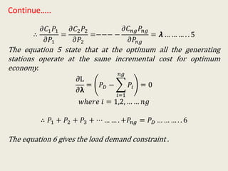
  • 13. Continue….. ∴ 𝜕𝐶1 𝑃1 𝜕𝑃1 = 𝜕𝐶2 𝑃2 𝜕𝑃2 =−−− − 𝜕𝐶 𝑛𝑔 𝑃𝑛𝑔 𝜕𝑃𝑛𝑔 = 𝞴 … … … . . 5 The equation 5 state that at the optimum all the generating stations operate at the same incremental cost for optimum economy. 𝜕L 𝜕𝝺 = 𝑃 𝐷 − 𝑖=1 𝑛𝑔 𝑃𝑖 = 0 𝑤ℎ𝑒𝑟𝑒 𝑖 = 1,2, … … 𝑛𝑔 ∴ 𝑃1 + 𝑃2 + 𝑃3 + ⋯ … … . +𝑃𝑛𝑔 = 𝑃 𝐷 … … … . . 6 The equation 6 gives the load demand constraint .
  • 14. Numerical No-1 Consider the power system with two stations. The incremental productions cost characteristics for the two stations are, 𝜕𝐹1 𝜕𝑃1 = 27.5 + 0.15𝑃1 𝑅𝑠/𝑀𝑤𝐻𝑟 𝜕𝐹2 𝜕𝑃2 = 19.5 + 0.26𝑃2 𝑅𝑠/𝑀𝑤𝐻𝑟 Given the minimum and maximum powers are to 10 MW and 100 MW at each plant. Schedule the generation at each plant to supply system load given by the load curve as below. Midnight Midnight 12 6 12 3 6 10 12 50 100 150 200
  • 15. 𝑪𝒂𝒔𝒆 𝟏 − 𝑃 𝐷 = 𝑃1 + 𝑃2 𝑷 𝟏 + 𝑷 𝟐 = 𝟓𝟎 𝑴𝑾 𝑻𝒊𝒎𝒆 − 𝟏𝟐 𝒕𝒐 𝟔 & 𝟏𝟎 𝒕𝒐 𝟏𝟐 … … . 𝟏 𝜕𝐹1 𝜕𝑃1 = 𝜕𝐹2 𝜕𝑃2 = 𝞴𝑅𝑠/𝑀𝑊𝐻𝑟 27.5 + 0.15𝑃1 = 19.5 + 0.26𝑃2 0.15𝑃1 − 0.26𝑃2 = −8 … … . . 2 S𝑜𝑙𝑣𝑒 𝑒𝑞𝑢𝑎𝑡𝑖𝑜𝑛 1 𝑎𝑛𝑑 2 𝑷 𝟏 = 𝟏𝟐. 𝟐 𝑴𝑾 & 𝑷 𝟐 = 𝟑𝟕. 𝟖 𝐌𝐖 𝞴 = 29.33 𝑅𝑠/𝑀𝑊𝐻𝑟 𝑪𝒂𝒔𝒆 𝟐 − 𝑃 𝐷 = 𝑃1 + 𝑃2 𝑷 𝟏 + 𝑷 𝟐 = 𝟏𝟎𝟎 𝑴𝑾 𝑻𝒊𝒎𝒆 − 𝟔 𝒕𝒐 𝟏𝟐 … … . 𝟑 𝜕𝐹1 𝜕𝑃1 = 𝜕𝐹2 𝜕𝑃2 = 𝞴𝑅𝑠/𝑀𝑊𝐻𝑟 27.5 + 0.15𝑃1 = 19.5 + 0.26𝑃2 0.15𝑃1 − 0.26𝑃2 = −8 … … . . 4 S𝑜𝑙𝑣𝑒 𝑒𝑞𝑢𝑎𝑡𝑖𝑜𝑛 3 𝑎𝑛𝑑 4 𝑷 𝟏 = 𝟒𝟑. 𝟗𝟎 𝑴𝑾 & 𝑷 𝟐 = 𝟓𝟔. 𝟏 𝐌𝐖 𝞴 = 34.08 𝑅𝑠/𝑀𝑊𝐻𝑟
  • 16. 𝑪𝒂𝒔𝒆 𝟑 − 𝑃 𝐷 = 𝑃1 + 𝑃2 𝑷 𝟏 + 𝑷 𝟐 = 𝟏𝟐𝟓 𝑴𝑾 𝑻𝒊𝒎𝒆 − 𝟏𝟐 𝒕𝒐 𝟑 … … . 𝟓 𝜕𝐹1 𝜕𝑃1 = 𝜕𝐹2 𝜕𝑃2 = 𝞴𝑅𝑠/𝑀𝑊𝐻𝑟 27.5 + 0.15𝑃1 = 19.5 + 0.26𝑃2 0.15𝑃1 − 0.26𝑃2 = −8 … … . . 6 S𝑜𝑙𝑣𝑒 𝑒𝑞𝑢𝑎𝑡𝑖𝑜𝑛 5 𝑎𝑛𝑑 6 𝑷 𝟏 = 𝟓𝟗. 𝟕𝟔 𝑴𝑾 & 𝑷 𝟐 = 𝟔𝟓. 𝟐𝟒 𝐌𝐖 𝞴 = 36.55 𝑅𝑠/𝑀𝑊𝐻𝑟 𝑪𝒂𝒔𝒆 𝟒 − 𝑃 𝐷 = 𝑃1 + 𝑃2 𝑷 𝟏 + 𝑷 𝟐 = 𝟏𝟓𝟎 𝑴𝑾 𝑻𝒊𝒎𝒆 − 𝟔 𝒕𝒐 𝟏𝟎 … … . 𝟕 𝜕𝐹1 𝜕𝑃1 = 𝜕𝐹2 𝜕𝑃2 = 𝞴𝑅𝑠/𝑀𝑊𝐻𝑟 27.5 + 0.15𝑃1 = 19.5 + 0.26𝑃2 0.15𝑃1 − 0.26𝑃2 = −8 … … . . 8 S𝑜𝑙𝑣𝑒 𝑒𝑞𝑢𝑎𝑡𝑖𝑜𝑛 7 𝑎𝑛𝑑 8 𝑷 𝟏 = 𝟕𝟓. 𝟔𝟏 𝑴𝑾 & 𝑷 𝟐 = 𝟕𝟒. 𝟑𝟗 𝐌𝐖 𝞴 = 38.84 𝑅𝑠/𝑀𝑊𝐻𝑟
  • 17. 𝑪𝒂𝒔𝒆 𝟓 − 𝑃 𝐷 = 𝑃1 + 𝑃2 𝑷 𝟏 + 𝑷 𝟐 = 𝟐𝟎𝟎 𝑴𝑾 𝑻𝒊𝒎𝒆 − 𝟑 𝒕𝒐 𝟔 … … . 𝟗 𝜕𝐹1 𝜕𝑃1 = 𝜕𝐹2 𝜕𝑃2 = 𝞴𝑅𝑠/𝑀𝑊𝐻𝑟 27.5 + 0.15𝑃1 = 19.5 + 0.26𝑃2 0.15𝑃1 − 0.26𝑃2 = −8 … … . . 10 S𝑜𝑙𝑣𝑒 𝑒𝑞𝑢𝑎𝑡𝑖𝑜𝑛 9 𝑎𝑛𝑑 10 𝑷 𝟏 = 𝟏𝟎𝟕. 𝟑𝟐 𝑴𝑾 & 𝑷 𝟐 = 𝟗𝟐. 𝟔𝟖 𝐌𝐖 𝞴 = 43.59 𝑅𝑠/𝑀𝑊𝐻𝑟 𝐼𝑓 𝑚𝑎𝑥𝑖𝑚𝑢𝑚 𝑔𝑒𝑛𝑒𝑟𝑎𝑡𝑖𝑜𝑛 𝑙𝑖𝑚𝑖𝑡 𝑜𝑓 100 𝑀𝑊 𝑖𝑠 𝑖𝑚𝑝𝑜𝑠𝑒𝑑 𝑡ℎ𝑒𝑛 𝑷 𝟏 = 𝟏𝟎𝟎 𝑴𝑾 & 𝑷 𝟐 = 𝟏𝟎𝟎 𝐌𝐖
  • 18. Numerical No-2 Consider the power system with two stations. The incremental productions cost characteristics for the two stations are, 𝜕𝐹1 𝜕𝑃1 = 220 + 1.32𝑃1 𝑅𝑠/𝑀𝑤𝐻𝑟 𝜕𝐹2 𝜕𝑃2 = 132 + 1.76𝑃2 𝑅𝑠/𝑀𝑤𝐻𝑟 Given the minimum and maximum powers are to 10 MW and 100 MW at each plant. Schedule the generation at each plant to supply system load given by the load curve as below. Midnight Midnight 12 6 12 3 6 10 12 50 100 150 200
  • 19. 𝑪𝒂𝒔𝒆 𝟏 − 𝑃 𝐷 = 𝑃1 + 𝑃2 𝑷 𝟏 + 𝑷 𝟐 = 𝟓𝟎 𝑴𝑾 𝑻𝒊𝒎𝒆 − 𝟏𝟐 𝒕𝒐 𝟔 & 𝟔 𝒕𝒐 𝟏𝟐 … … . 𝟏 𝜕𝐹1 𝜕𝑃1 = 𝜕𝐹2 𝜕𝑃2 = 𝞴𝑅𝑠/𝑀𝑊𝐻𝑟 220 + 1.32𝑃1 = 132 + 1.76𝑃2 1.32𝑃1 − 1.76𝑃2 = −88 … … . . 2 S𝑜𝑙𝑣𝑒 𝑒𝑞𝑢𝑎𝑡𝑖𝑜𝑛 1 𝑎𝑛𝑑 2 𝑷 𝟏 = 𝟎 𝑴𝑾 & 𝑷 𝟐 = 𝟒𝟗. 𝟗𝟔 𝐌𝐖 𝞴 = 220 𝑅𝑠/𝑀𝑊𝐻𝑟 𝐼𝑓 𝑚𝑖𝑛𝑖𝑚𝑢𝑚 𝑎𝑛𝑑 𝑚𝑎𝑥𝑖𝑚𝑢𝑚 𝑔𝑒𝑛𝑒𝑟𝑎𝑡𝑖𝑜𝑛 𝑙𝑖𝑚𝑖𝑡 𝑜𝑓 10𝑀𝑊 𝑎𝑛𝑑 100 𝑀𝑊 𝑟𝑒𝑠𝑝𝑒𝑐𝑡𝑖𝑣𝑒𝑙𝑦 𝑖𝑠 𝑖𝑚𝑝𝑜𝑠𝑒𝑑 𝑡ℎ𝑒𝑛 𝑷 𝟏 = 𝟏𝟎 𝑴𝑾 & 𝑷 𝟐 = 𝟒𝟎 𝐌𝐖
  • 20. 𝑪𝒂𝒔𝒆 𝟐 − 𝑃 𝐷 = 𝑃1 + 𝑃2 𝑷 𝟏 + 𝑷 𝟐 = 𝟐𝟎𝟎 𝑴𝑾 𝑻𝒊𝒎𝒆 − 𝟔 𝒕𝒐 𝟔 … … . 𝟑 𝜕𝐹1 𝜕𝑃1 = 𝜕𝐹2 𝜕𝑃2 = 𝞴𝑅𝑠/𝑀𝑊𝐻𝑟 220 + 1.32𝑃1 = 132 + 1.76𝑃2 1.32𝑃1 − 1.76𝑃2 = −88 … … . . 4 S𝑜𝑙𝑣𝑒 𝑒𝑞𝑢𝑎𝑡𝑖𝑜𝑛 3 𝑎𝑛𝑑 4 𝑷 𝟏 = 𝟖𝟓. 𝟕 𝑴𝑾 & 𝑷 𝟐 = 𝟏𝟏𝟒. 𝟑 𝐌𝐖 𝞴 = 333.12 𝑅𝑠/𝑀𝑊𝐻𝑟 𝐼𝑓 𝑚𝑖𝑛𝑖𝑚𝑢𝑚 𝑎𝑛𝑑 𝑚𝑎𝑥𝑖𝑚𝑢𝑚 𝑔𝑒𝑛𝑒𝑟𝑎𝑡𝑖𝑜𝑛 𝑙𝑖𝑚𝑖𝑡 𝑜𝑓 10𝑀𝑊 𝑎𝑛𝑑 100 𝑀𝑊 𝑟𝑒𝑠𝑝𝑒𝑐𝑡𝑖𝑣𝑒𝑙𝑦 𝑖𝑠 𝑖𝑚𝑝𝑜𝑠𝑒𝑑 𝑡ℎ𝑒𝑛 𝑷 𝟏 = 𝟏𝟎𝟎 𝑴𝑾 & 𝑷 𝟐 = 𝟏𝟎𝟎 𝐌𝐖
  • 21. Transmission loss formula- 𝐵 𝑚𝑛 𝐶𝑜𝑒𝑓𝑓𝑖𝑐𝑖𝑒𝑛𝑡𝑠 Consider the power system with generator and load currents as shown in figure, For simplicity 𝑛𝑔 = 2, 𝐺1 𝐺2 𝐺 𝑛𝑔 𝑖 𝑔1 𝑖 𝑔2 𝑖 𝑔𝑛𝑔 𝑖 𝐿3 𝑖 𝐿2 𝑖 𝐿1 𝑃𝑜𝑤𝑒𝑟 𝑁𝑒𝑡𝑤𝑜𝑟𝑘 𝐼 𝐾 𝑁𝑒𝑡𝑤𝑜𝑟𝑘 𝐸𝑙𝑒𝑚𝑒𝑛𝑡 Now consider a network element K (an interconnected line in the system) carrying current 𝐼 𝐾. 𝐼 𝐾 = 𝐼 𝐾1 + 𝐼 𝐾2 Let the ratio of 𝐼 𝐾 and 𝐼𝑔 be 𝑑 𝐾1 = 𝐼 𝐾1 𝐼𝑔1 𝑎𝑛𝑑 𝑑 𝐾2 = 𝐼 𝐾2 𝐼𝑔2
  • 22. The power losses in the network comprising of 𝑛𝑔 network elements or branches 𝑃𝑙𝑜𝑠𝑠 is given by, 𝑃𝐿 = 𝐾=1 𝑛𝑔 3 𝐼 𝐾 2 𝑅 𝐾 … … … 1 𝑤ℎ𝑒𝑟𝑒 𝑅 𝐾is the resistance of element K. 𝐼 𝐾 2 = 𝑑 𝐾1 𝑃1 3 𝑉1 cos 𝜑1 2 + 𝑑 𝐾2 𝑃2 3 𝑉2 cos 𝜑2 2 + 2𝑑 𝐾1 𝑑 𝐾2 cos 𝛿1 − 𝛿2 3 𝑉1 𝑉2 cos 𝜑1 cos 𝜑2 … … 2 Substituting equation 2 in to 1 𝑃𝐿 = 𝑃1 2 𝐾=1 𝑛𝑔 𝑑 𝐾1 2 𝑅 𝐾 𝑉1 2 cos 𝜑1 2 + 𝑃2 2 𝐾=1 𝑛𝑔 𝑑 𝐾2 2 𝑅 𝐾 𝑉2 2 cos 𝜑2 2 + 2𝑃1 𝑃2 𝐾=1 𝑛𝑔 𝑑 𝐾1 𝑑 𝐾2 cos 𝛿1 − 𝛿2 3 𝑉1 𝑉2 cos 𝜑1 cos 𝜑2 … 3 𝑃𝐿 = 𝑃1 2 𝐵11 + 𝑃2 2 𝐵22 + 2𝑃1 𝑃2 𝐵12 𝑃𝐿 = 𝑚=1 2 𝑃𝑚 𝑛=1 2 𝑃𝑛 𝐵 𝑚𝑛
  • 23. Economic scheduling of thermal plants considering effect of transmission losses- 𝑇ℎ𝑒 𝑜𝑏𝑗𝑒𝑐𝑡𝑖𝑣𝑒 𝑓𝑢𝑛𝑐𝑡𝑖𝑜𝑛 𝑓𝑜𝑟 𝑐𝑜𝑠𝑡 𝑚𝑖𝑛𝑖𝑚𝑖𝑧𝑎𝑡𝑖𝑜𝑛 𝑖𝑠 𝑔𝑖𝑣𝑒𝑛 𝑎𝑠, 𝐹 𝑃𝑖 = 𝑖=1 𝑛𝑔 𝐶𝑖 𝑃𝑖 … … … … … .1 𝑤ℎ𝑒𝑟𝑒 𝑖 = 1,2, … … 𝑛𝑔 𝑇ℎ𝑒 𝑒𝑞𝑢𝑎𝑙𝑖𝑡𝑦 𝑐𝑜𝑛𝑠𝑡𝑟𝑎𝑖𝑛𝑡 𝑖𝑠 𝑔𝑖𝑣𝑒𝑛 𝑏𝑦 𝐺 𝑃𝑖 = 𝑃 𝐷 + 𝑃𝐿 − 𝑖=1 𝑛𝑔 𝑃𝑖 … … … … … 2 (𝑻𝒐𝒕𝒂𝒍 𝑺𝒖𝒑𝒑𝒍𝒚 = 𝒕𝒐𝒕𝒂𝒍 𝒅𝒆𝒎𝒂𝒏𝒅) 𝑻𝒉𝒆 𝑳𝒂𝒈𝒓𝒂𝒏𝒈𝒆 𝑭𝒖𝒏𝒄𝒕𝒊𝒐𝒏 𝒊𝒔 𝒈𝒊𝒗𝒆𝒏 𝒂𝒔, 𝑳 𝑷, 𝞴 = 𝑭 𝑷 + 𝞴𝑮 𝑷 … … … … … . 𝟑 𝑊ℎ𝑒𝑟𝑒 𝞴 𝑖𝑠 𝑙𝑎𝑔𝑟𝑎𝑛𝑔𝑒 𝑚𝑢𝑙𝑡𝑖𝑝𝑙𝑖𝑒𝑟.
  • 24. Continue….. Substitute equation 1, 2 in to 3, 𝑳 𝑷, 𝞴 = 𝑖=1 𝑛𝑔 𝐶𝑖 𝑃𝑖 + 𝞴 𝑃 𝐷 + 𝑃𝐿 − 𝑖=1 𝑛𝑔 𝑃𝑖 … … … . . 4 𝑇ℎ𝑒 𝑛𝑒𝑐𝑒𝑠𝑠𝑎𝑟𝑦 𝑐𝑜𝑛𝑑𝑖𝑡𝑖𝑜𝑛𝑠 𝑎𝑟𝑒 𝑔𝑖𝑣𝑒𝑛 𝑎𝑠, 𝜕L 𝜕Pi = 0 & 𝜕𝐿 𝜕𝝺 = 0 Now apply above conditions on equation 4 , 𝜕L 𝜕Pi = 𝜕𝐶𝑖 𝑃𝑖 𝜕Pi + 𝞴 𝜕𝑃𝐿 𝜕Pi + 𝞴 −1 = 0 𝑤ℎ𝑒𝑟𝑒 𝑖 = 1,2, … … 𝑛𝑔
  • 25. Continue….. 𝜕𝐶𝑖 𝑃𝑖 𝜕Pi + 𝞴 𝜕𝑃𝐿 𝜕Pi = 𝞴 … … … . . 5 The equation 5 state that the sum of the incremental production cost of power at any plant i and the incremental transmission losses incurred due to generation 𝑃𝑖 at the rate of 𝞴 𝑚𝑢𝑠𝑡 𝑏𝑒 𝑐𝑜𝑛𝑠𝑡𝑎𝑛𝑡 𝑓𝑜𝑟 𝑎𝑙𝑙 𝑔𝑒𝑛𝑒𝑟𝑎𝑡𝑜𝑟𝑠 𝑎𝑛𝑑 𝑒𝑞𝑢𝑎𝑙 𝑡𝑜 𝞴. 𝜕L 𝜕𝝺 = 𝑃 𝐷 + 𝑃𝐿 − 𝑖=1 𝑛𝑔 𝑃𝑖 = 0 𝑤ℎ𝑒𝑟𝑒 𝑖 = 1,2, … … 𝑛𝑔 ∴ 𝑃1 + 𝑃2 + 𝑃3 + ⋯ … … . +𝑃𝑛𝑔 = 𝑃 𝐷 + 𝑃𝐿 … … … . . 6 The equation 6 gives the load demand constraint .
  • 26. Penalty Factor- 𝜕𝐶𝑖 𝑃𝑖 𝜕Pi + 𝞴 𝜕𝑃𝐿 𝜕Pi = 𝞴 𝑤ℎ𝑒𝑟𝑒 𝑖 = 1,2, … … 𝑛𝑔 𝞴 = 𝜕𝐶𝑖 𝑃𝑖 𝜕Pi 1 − 𝜕𝑃𝐿 𝜕Pi When transmission losses are included , the incremental production cost at each plant ‘i ‘ must be multiplied by a factor 1 1− 𝜕𝑃 𝐿 𝜕Pi which then will be equal to the incremental cost of power delivered. Hence the factor 1 1− 𝜕𝑃 𝐿 𝜕Pi is called Penalty Factor.
  • 27. Numerical No-3 Given a two bus system as shown in figure. The incremental productions cost characteristics for the two stations are, 𝜕𝐹1 𝜕𝑃1 = 15 + 0.03𝑃1 𝑅𝑠/𝑀𝑤𝐻𝑟 𝜕𝐹2 𝜕𝑃2 = 18 + 0.05𝑃2 𝑅𝑠/𝑀𝑤𝐻𝑟 It is observed that when a power of 75 MW is imported to bus 1, the loss amounted to 5 MW. Find the generation needed from each plant and also the power received by the load, if the system 𝞴 𝑖𝑠 𝑔𝑖𝑣𝑒𝑛 𝑏𝑦 20𝑅𝑆/𝑀𝑊𝐻𝑟. G1 G2 200𝑀𝑊 75 𝑀𝑊 Load 1 2 Line
  • 28. Solution- The power loss equation is given as, 𝑃𝐿 = 𝑃1 2 𝐵11 + 𝑃2 2 𝐵22 + 2𝑃1 𝑃2 𝐵12 The load is at bus 1, hence 𝑃1 will no have any effect on the line losses. Therefore 𝐵11 = 𝐵12 = 𝐵21 = 0 𝑷 𝑳 = 𝑷 𝟐 𝟐 𝑩 𝟐𝟐 … … 𝟐 when a power of 75 MW is imported to bus 1, the loss amounted to 5 MW. 𝟓 = 𝑩 𝟐𝟐 ∗ 𝟕𝟓 𝟐 𝑩 𝟐𝟐 = 𝟖. 𝟗 ∗ 𝟏𝟎−𝟒 = 𝟎. 𝟎𝟎𝟎𝟖𝟗 Equation 2 becomes, 𝑷 𝑳 = 𝟎. 𝟎𝟎𝟎𝟖𝟗𝑷 𝟐 𝟐 … … 𝟑 𝛛𝑷 𝑳 𝛛𝑷 𝟏 = 𝟎 𝐚𝐧𝐝 𝛛𝑷 𝑳 𝛛𝑷 𝟐 = 𝟐 ∗ 𝟎. 𝟎𝟎𝟎𝟖𝟗 ∗ 𝑷 𝟐
  • 29. Now consider at station 1- 𝛛𝑷 𝑳 𝛛𝑷 𝟏 = 𝟎 𝜕𝐶1 𝑃1 𝜕P1 + 𝞴 𝜕𝑃𝐿 𝜕P1 = 𝞴 15 + 0.03𝑃1 + 𝞴 ∗ 0 = 𝞴 𝞴 = 20 𝑅𝑆/𝑀𝑊𝐻𝑟 𝑷 𝟏 = 𝟏𝟔𝟔. 𝟔𝟕 𝑴𝑾
  • 30. Now consider at station 2- 𝛛𝑷 𝑳 𝛛𝑷 𝟐 = 𝟐 ∗ 𝟎. 𝟎𝟎𝟎𝟖𝟗 ∗ 𝑷 𝟐 𝜕𝐶2 𝑃2 𝜕P2 + 𝞴 𝜕𝑃𝐿 𝜕P2 = 𝞴 18 + 0.05𝑃2 + 𝞴 ∗ 𝟐 ∗ 𝟎. 𝟎𝟎𝟎𝟖𝟗 ∗ 𝑷 𝟐 = 𝞴 𝞴 = 20 𝑅𝑆/𝑀𝑊𝐻𝑟 𝑷 𝟐 = 𝟐𝟑. 𝟑𝟔 𝑴𝑾
  • 31. Total Transmission loss is when 𝑷 𝟐 = 𝟐𝟑. 𝟑𝟔 𝑴𝑾 is transmitted from bus 2 to the load connected at bus 1 is given as 𝑷 𝑳 = 𝟎. 𝟎𝟎𝟎𝟖𝟗𝑷 𝟐 𝟐 𝑷 𝑳 = 𝟎. 𝟎𝟎𝟎𝟖𝟗 ∗ 𝟐𝟑. 𝟑𝟔 𝟐 𝑷 𝑳 = 𝟎. 𝟒𝟖𝟓𝟖 𝐌𝐖 The total load demand at bus 1 is 𝑷 𝑫 = 𝑷 𝟏 + 𝑷 𝟐 − 𝑷 𝑳 𝑷 𝑫 = 𝟏𝟔𝟔. 𝟔𝟕 + 𝟐𝟑. 𝟑𝟔 − 𝟎. 𝟒𝟖𝟓𝟖 𝑷 𝑫 = 𝟏𝟖𝟗. 𝟓𝟒 𝑴𝑾
  • 32. Unit Commitment- The topic of unit commitment deals with specifying the units which should be operated for a given load . That means which units should be committed to supply a given load. It is economical to de-commit certain units when load is low. “To commit a unit means to bring the boiler to the required temperature, bring the turbine and generator to synchronous speed and synchronise the generator to the system”.
  • 33. Constraints in Unit Commitment- The problem of deciding which units to for a certain load is beset with many constraints,  Spinning Reserve  Minimum up time  Minimum down time  Crew Constraints  Transition cost  Hydro Constraints  Nuclear Constraints  Must runtime Units  Fuel Supply Constraints
  • 34. Methods of Unit Commitment- 1. Priority List Methods In this method we prepare priority list of the order in which the generating units should be added to the system. This list would also include the order of the shutting down the units when the system load decreases. When the load is very low, the units with the lowest heat rate supplies the entire load. As the load increases the units having heat rates in ascending order are successively added.
  • 35. Consider the three thermal plants operating with the following incremental fuel rate characteristics, Plant 1 𝐹1 = 7 + 0.003𝑃1 ∗ 103 𝐾 − 𝐶𝑎𝑙/𝑀𝑤𝐻𝑟 𝑃1 𝑚𝑎𝑥 = 500 𝑀𝑊 & 𝑃1 𝑚𝑖𝑛 = 50 𝑀𝑊 Plant 2 𝐹2 = 7.5 + 0.002𝑃2 ∗ 103 𝐾 − 𝐶𝑎𝑙/𝑀𝑤𝐻𝑟 𝑃2 𝑚𝑎𝑥 = 400 𝑀𝑊 & 𝑃2 𝑚𝑖𝑛 = 40 𝑀𝑊 Plant 3 𝐹3 = 8 + 0.004𝑃3 ∗ 103 𝐾 − 𝐶𝑎𝑙/𝑀𝑤𝐻𝑟 𝑃3 𝑚𝑎𝑥 = 200 𝑀𝑊 & 𝑃3 𝑚𝑖𝑛 = 20 𝑀𝑊 The fuel cost at the plant is given as 𝐶𝑃1 = 1.1 𝑅𝑆/𝐾𝑐𝑎𝑙 𝐶𝑃2 = 1.05 𝑅𝑆/𝐾𝑐𝑎𝑙 𝐶𝑃3 = 1.2 𝑅𝑆/𝐾𝑐𝑎𝑙
  • 36. The full load average production cost is Plant 1- 𝑃1 𝑚𝑎𝑥 = 500 𝑀𝑊 𝐹1 ∗ 𝐶𝑃1 = 7 + 0.003 ∗ 500 ∗ 103 ∗ 1.1 𝑅𝑆/𝑀𝑤𝐻𝑟 = 𝟗. 𝟑𝟓 ∗ 𝟏𝟎 𝟑 𝑹𝑺/𝑴𝒘𝑯𝒓 Plant 2 𝑃2 𝑚𝑎𝑥 = 400 𝑀𝑊 𝐹2 ∗ 𝐶𝑃2 = 7.5 + 0.002 ∗ 400 ∗ 103) ∗ 1.05 𝑅𝑆/𝑀𝑤𝐻𝑟 = 𝟖. 𝟕𝟏𝟓 ∗ 𝟏𝟎 𝟑 𝑹𝑺/𝑴𝒘𝑯𝒓 Plant 3 𝑃3 𝑚𝑎𝑥 = 200 𝑀𝑊 𝐹3 ∗ 𝐶𝑃3 = 8 + 0.004 ∗ 200 ∗ 103 ∗ 1.2 𝑅𝑆/𝑀𝑤𝐻𝑟 = 𝟏𝟎. 𝟓𝟔 ∗ 𝟏𝟎 𝟑 𝑹𝑺/𝑴𝒘𝑯𝒓
  • 37. The priority list for supplying load up to 1000 MW is prepared as, Units Maximum(MW) Minimum(MW) 2,1,3 1000 110 2,1 900 90 2 400 40 In order of increasing cost the following table is constructed as, Unit RS/MWHr Maximum(MW) Minimum(MW) 2 𝟖. 𝟕𝟏𝟓 ∗ 𝟏𝟎 𝟑 400 40 1 𝟗. 𝟑𝟓 ∗ 𝟏𝟎 𝟑 500 50 3 𝟏𝟎. 𝟓𝟔 ∗ 𝟏𝟎 𝟑 200 20
  • 38. Methods of Unit Commitment- 2. Dynamic Programming This method can be applied to problems in which many sequential decisions are required to be taken in defining the optimum operation of a system or process composed of distinct number of stages. However , it is suitable only when the decisions at later stages do not affect the operation at the earlier stages.
  • 39. Let the cost of operating the first unit be 𝐹1 𝑃1 when supplying power 𝑃1is , 𝑭 𝟏 𝑷 𝟏 = 𝑓1 𝑝1 The optimal combination of this unit with a second unit can be derived next to supply a load of 𝑃1 + 𝑃2 for which the optimal cost is 𝐹2 𝑃1 + 𝑃2 = min[𝑓2 𝑝2 + 𝑭 𝟏 𝑷 𝟏 ] As 𝐹1 𝑃1 is already the optimal value, the best units to supply 𝑃2 from the rest of (N-1) units will be picked during second stage of optimization for lowest possible cost of production. 𝐹3 𝑃1 + 𝑃2 + 𝑃3 = min[𝑓3 𝑝3 + 𝐹2 𝑃1 + 𝑃2 ] In general 𝐹 𝑁 𝑖=1 𝑁 𝑃𝑖 = min[𝐹 𝑁 𝑃 𝑁 + 𝐹 𝑁−1 𝑃𝑛 𝑖=1 𝑁−1 𝑃𝑖
  • 40. Numerical-4 Obtain the economic schedule for the two units , the production cost of which are given as follows, to supply a load of 3 MW , in steps of 1 MW. 𝐹1 = 0.8𝑃1 2 + 25𝑃1 𝐹2 = 1.2𝑃2 2 + 22𝑃2 Using Dynamic Programming. Solution- 𝐹1 3 = 0.8 ∗ 32 + 25 ∗ 3 = 82.2 𝑭 𝟐 𝟑 = 𝐦𝐢𝐧[𝒇 𝟐 𝟎 + 𝒇 𝟏 𝟑 , 𝒇 𝟐 𝟏 + 𝒇 𝟏 𝟐 , 𝒇 𝟐 𝟐 + 𝒇 𝟏 𝟏 , 𝒇 𝟐 𝟑 + 𝒇 𝟏 𝟎 ] 𝑓1 2 = 0.8 ∗ 22 + 25 ∗ 2 = 53.2 𝑓1 1 = 0.8 ∗ 12 + 25 ∗ 1 = 25.8 𝑓1 0 = 0.8 ∗ 02 + 25 ∗ 0 = 0 𝑓2 3 = 1.2 ∗ 32 + 22 ∗ 3 = 76.8 𝑓2 3 = 1.2 ∗ 22 + 22 ∗ 2 = 48.8 𝑓2 1 = 1.2 ∗ 12 + 22 ∗ 1 = 23.2 𝑓2 0 = 1.2 ∗ 02 + 22 ∗ 0 = 0
  • 41. 𝐹1 3 = 82.2, 𝑓1 2 = 53.2, 𝑓1 1 = 25.8, 𝑓1 0 = 0 𝑓2 3 = 76.8, 𝑓2 2 = 48.8 , 𝑓2 1 = 23.2, 𝑓2 0 = 0 𝑭 𝟐 𝟑 = 𝐦𝐢𝐧[𝒇 𝟐 𝟎 + 𝒇 𝟏 𝟑 , 𝒇 𝟐 𝟏 + 𝒇 𝟏 𝟐 , 𝒇 𝟐 𝟐 + 𝒇 𝟏 𝟏 , 𝒇 𝟐 𝟑 + 𝒇 𝟏 𝟎 ] 𝑭 𝟐 𝟑 = 𝐦𝐢𝐧[ 𝟎 + 𝟖𝟐. 𝟐, 𝟐𝟑. 𝟐 + 𝟓𝟑. 𝟐, 𝟒𝟖. 𝟖 + 𝟐𝟓. 𝟖, 𝟕𝟔. 𝟖 + 𝟎] 𝑭 𝟐 𝟑 = 𝐦𝐢𝐧[ 𝟖𝟐. 𝟐, 𝟕𝟔. 𝟒, 𝟕𝟒. 𝟔, 𝟕𝟔. 𝟖] The most economical combination is unit 2 supplying 2 MW and unit supplying 1 MW.