


![Robot Arm Domain Y 1 Y 2 Two-link, two-joint robot arm Link 1 extendible: L 1 [2, 10] Y 1 = L 1 sin( 1 ) Y 2 = L 1 sin( 1 ) + 5 sin( 1 + 2 ) 1 2 Four learning problems: A: Y 1 = f(L 1 , 1 ) B: Y 2 = f(L 1 , 1 , 2 , sum , Y 1 ) C: Y 2 = f(L 1 , 1 , 2 , sum ) D: Y 2 = f(L 1 , 1 , 2 ) L 1 Derived attribute sum = 1 + 2 Difficulty for Q 2](https://image.slidesharecdn.com/using-qualitative-knowledge-in-numerical-learning3245/85/Using-Qualitative-Knowledge-in-Numerical-Learning-80-320.jpg)


Using Qualitative Knowledge in Numerical Learning
- 1. USING QUALITATIVE KNOWLEDGE IN NUMERICAL LEARNING Ivan Bratko Faculty of Computer and Info. Sc. University of Ljubljana Slovenia
- 2. THIS TALK IS ABOUT: AUTOMATED MODELLING FROM DATA WITH MACHINE LEARNING COMBINING NUMERICAL AND QUALITATIVE REPRESENTATIONS
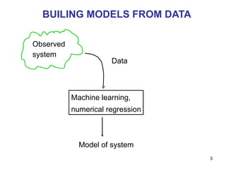
- 3. BUILING MODELS FROM DATA Observed system Machine learning, numerical regression Model of system Data
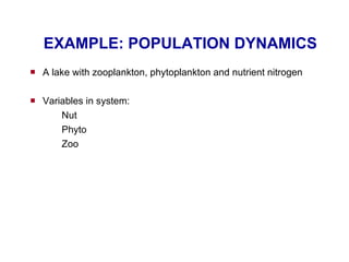
- 4. EXAMPLE: POPULATION DYNAMICS A lake with zooplankton, phytoplankton and nutrient nitrogen Variables in system: Nut Phyto Zoo
- 5. POPULATION DYNAMICS Observed behaviour in time Data provided by Todorovski&D žeroski
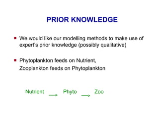
- 6. PRIOR KNOWLEDGE We would like our modelling methods to make use of expert’s prior knowledge (possibly qualitative) Phytoplankton feeds on Nutrient, Zooplankton feeds on Phytoplankton Nutrient Phyto Zoo
- 7. QUALITATIVE DIFFICULTIES OF NUMERICAL LEARNING Learn time behavior of water level: h = f( t, initial_outflow) Level h outflow t h
- 8. TIME BEHAVIOUR OF WATER LEVEL Initial_ouflow =12.5
- 9. VARYING INITIAL OUTFLOW Initial_ouflow =12.5 11.25 10.0 8.75 6.25
- 10. PREDICTING WATER LEVEL WITH M5 11.25 10.0 8.75 6.25 7.5 Initial_ouflow =12.5 Qualitatively incorrect – water level cannot increase M5 prediction
- 11. QUALITATIVE ERRORS OF NUMERICAL LEARNERS E xperiments with regression (model) trees ( M5; Quinlan 92 ) , LWR (Atkenson et.al. 97) in Weka ( Witten & Frank 2000 ) , neural nets, ... Qualitative errors: water level should never increase water level should not be negative An expert might accept numerical errors, but such qualitative errors are particularly disturbing
- 12. Q 2 LEARNING AIMS AT OVERCOMING THESE DIFFICULTIES
- 13. Q 2 LEARNING Š uc, Vladu š i č , Bratko; IJCAI’03, AIJ 2004, IJCAI’05 Aims at overcoming these difficulties of numerical learning Q 2 = Q ualitatively faithful Q uantitative learning Q 2 makes use of qualitative constraints
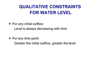
- 14. QUALITATIVE CONSTRAINTS FOR WATER LEVEL For any initial outflow: Level is always decreasing with time For any time point: Greater the initial outflow, greater the level
- 15. SUMMARY OF Q 2 LEARNING Standard numerical learning approaches make qualitative errors. As a result, numerical predictions are qualitatively inconsistent with expectations Q 2 learning (Qualitatively faithful Quantitative prediction); A method that enforces qualitative consistency Resulting numerical models enable clearer interpretation, and also significantly improve quantitative prediction
- 16. IDEA OF Q 2 First find qualitative laws in data Respect these qualitative laws in numerical learning
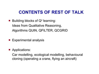
- 17. CONTENTS OF REST OF TALK Building blocks of Q 2 learning: Ideas from Qualitative Reasoning, Algorithms QUIN, QFILTER, QCGRID Experimental analysis Applications: Car modelling, ecological modelling, behavioural cloning (operating a crane, flying an aircraft)
- 18. HOW CAN WE DESCRIBE QUALITATIVE PROPERTIES ? We can use concepts from field of qualitative reasoning in AI Related terms: Qualitative physics, Naive physics, Qualitative modelling
- 19. QUALITATIVE MODELLING IN AI Naive physics, as opposed to "proper physics“ Qualitative modelling, as opposed to quantitative modelling
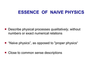
- 20. ESSENCE OF NAIVE PHYSICS Describe physical processes qualitatively , without numbers or exact numerical relations “ Naive physics”, as opposed to "proper physics“ Close to common sense descriptions
- 21. EXAMPLE: BATH TUB What will happen? Amount of water will keep increasing, so will level, until the level reaches the top.
- 22. EXAMPLE: U-TUBE What will happen? La Lb Level La will be decreasing, and Lb increasing, until La = Lb.
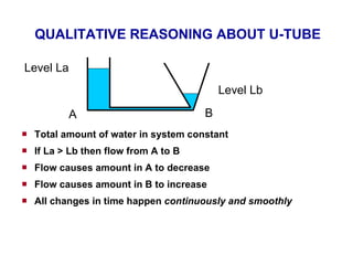
- 23. QUALITATIVE REASONING ABOUT U-TUBE Total amount of water in system constant If La > Lb then flow from A to B Flow causes amount in A to decrease Flow causes amount in B to increase All changes in time happen continuously and smoothly Level La Level Lb A B
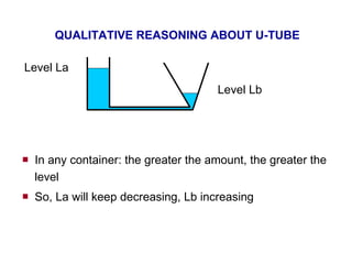
- 24. QUALITATIVE REASONING ABOUT U-TUBE In any container: the greater the amount, the greater the level So, La will keep decreasing, Lb increasing Level La Level Lb
- 25. QUALITATIVE REASONING ABOUT U-TUBE La will keep decreasing, Lb increasing, until they equalise Level La Level Lb La Lb Time
- 26. THIS REASONING IS VALID FOR ALL CONTAINERS OF ANY SHAPE AND SIZE, REGARDLESS OF ACTUAL NUMBERS!
- 27. QHY REASON QUALITATIVELY? Because it is easier than quantitatively Because it is easy to understand - facilitates explanation We want to exploit these advantages in ML
- 28. RELATION BETWEEN AMOUNT AND LEVEL The greater the amount, the greater the level A = M + (L) A is a monotonically increasing function of L
- 29. MONOTONIC FUNCTIONS Y = M + (X) specifies a family of functions X Y
- 30. MONOTONIC QUALITATIVE CONSTRAINTS, MQCs Generalisation of monotonically increasing functions to several arguments Example: Z = M +,- ( X, Y) Z increases with X, and decreases with Y More precisely: if X increases and Y stays unchanged then Z increases
- 31. EXAMPLE: BEHAVIOUR OF GAS Pressure = M +,- (Temperature, Volume) Pressure increases with Temperature Pressure decreases with Volume
- 32. Q 2 LEARNING Induce qualitative constraints ( QUIN ) Qualitative to Quantitative Transformation (Q2Q) Numerical predictor : respects qualitative constraints fits data numerically Numerical data One possibility: QFILTER
- 33. PROGRAM QUIN INDUCING QUALITATIVE CONSTRAINTS FROM NUMERICAL DATA Šuc 2001 ( PhD Thesis , also as book 2003 ) Šuc and Bratko, ECML ’ 01
- 34. QUIN QUIN = Qualitative Induction Numerical examples QUIN Qualitative tree Qualitative tree : similar to decision tree, qualitative constraints in leaves
- 35. EXAMPLE PROBLEM FOR QUIN Noisy examples: z = x 2 - y 2 + noise(st.dev. 50)
- 36. EXAMPLE PROBLEM FOR QUIN In this region: z = M +,+ (x,y)
- 37. INDUCED QUALITATIVE TREE FOR z = x 2 - y 2 + noise z= M -,+ ( x,y) z= M -,- ( x,y) z= M +,+ ( x , y) z= M +,- ( x,y) 0 > 0 > 0 0 > 0 0 y x y
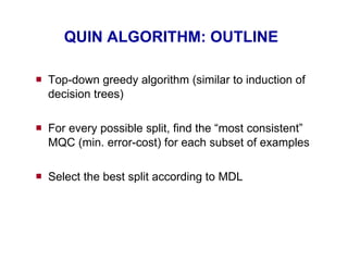
- 38. QUIN ALGORITHM: OUTLINE Top-down greedy algorithm (similar to induction of decision trees) For every possible split, find the “most consistent” MQC (min. error-cost) for each subset of examples Select the best split according to MDL
- 39. Q2Q Qualitative to Quantitative Transformation
- 40. Q2Q EXAMPLE X < 5 y n Y = M + (X) Y = M - (X) 5 X Y
- 41. QUALITATIVE TREES IMPOSE NUMERICAL CONSTRAINTS MQCs impose numerical constraints on class values, between pairs of examples y = M + (x) requires: If x 1 > x 2 then y 1 > y 2
- 42. RESPECTING MQCs NUMERICALLY z = M +,+ (x,y) requires: If x 1 < x 2 and y 1 < y 2 then z 1 < z 2 (x 2 , y 2 ) (x 1 , y 1 ) x y
- 43. QFILTER AN APPROACH TO Q2Q TRANSFORMATION Šuc and Bratko, ECML ’03
- 44. TASK OF QFILTER Given: qualitative tree points with class predictions by arbitrary numerical learner learning examples (optionally) Modify class predictions to achieve consistency with qualitative tree
- 45. QFILTER IDEA Force numerical predictions to respect qualitative constraints : find minimal changes of predicted values so that qualitative constraints become satisfied “ minimal” = min. sum of squared changes a quadratic programming problem
- 46. RESPECTING MQCs NUMERICALLY Y = M + (X) X Y
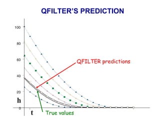
- 47. QFILTER APPLIED TO WATER OUTFLOW Qualitative constraint that applies to water outflow: h = M -,+ (time, InitialOutflow) This could be supplied by domain expert, or induced from data by QUIN
- 48. PREDICTING WATER LEVEL WITH M5 7.5 M5 prediction
- 49. QFILTER’S PREDICTION QFILTER predictions T rue values
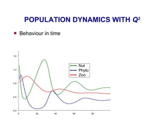
- 50. POPULATION DYNAMICS Aquatic ecosystem with zooplankton, phytoplankton and nutrient nitrogen Phyto feeds on Nutrient, Zoo feeds on Phyto Nutrient Phyto Zoo
- 51. POPULATION DYNAMICS WITH Q 2 Behaviour in time
- 52. PREDICTION PROBLEM Predict the change in zooplankton population: ZooChange(t) = Zoo(t + 1) - Zoo(t) Biologist’s rough idea: ZooChange = Growth - Mortality M +,+ (Zoo, Phyto) M + (Zoo)
- 53. APPROXIMATE QUALITATIVE MODEL OF ZOO CHANGE Induced from data by QUIN
- 54. EXPERIMENT WITH NOISY DATA All results as MSE (Mean Squared Error) 2.269 ; 1.889 0.112 ; 0.102 0.015 ; 0.008 ZooChange 20 % noise LWR; Q 2 5 % noise LWR; Q 2 no noise LWR; Q 2 Domain
- 55. APPLICATIONS OF Q 2 FROM REAL ECOLOGICAL DATA Growth of algae Lagoon of Venice Plankton in Lake Glumsoe
- 56. Lake Glumsø Location and properties: Lake Glumsø is located in a sub-glacial valley in Denmark Average depth 2 m Surface area 266000 m 2 Pollution Receives waste water from community with 3000 inhabitants (mainly agricultural) High nitrogen and phosphorus concentration in waste water caused hypereutrophication No submerged vegetation low transparency of water oxygen deficit at the bottom of the lake
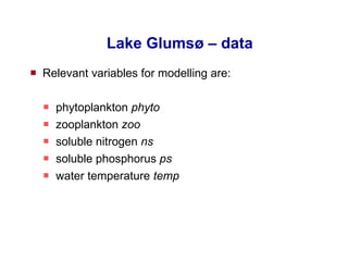
- 57. Lake Glumsø – data Relevant variables for modelling are: phytoplankton phyto zooplankton zoo soluble nitrogen ns soluble phosphorus ps water temperature temp
- 58. PREDICTION ACCURACY Over all (40) experiments. Q 2 better than LWR in 75% (M5, 83%) of the test cases The differences were found significant (t-test) at 0.02 significance level
- 59. OTHER ECOLOGICAL MODELLING APPLICATIONS Predicting ozone concentrations in Ljubljana and Nova Gorica Predicting flooding of Savinja river Q2 model by far superior to any predictor so far used in practice
- 60. CASE STUDY INTEC’S CAR SIMULATION MODELS Goal: simplify INTEC’s car models to speed up simulation Context: Clockwork European project (engineering design)
- 62. Learning Manouvres Learning manouvres were very simple: Sinus bump Turning left Turning right Road excitation: Steering position
- 63. WHEEL MODEL : PREDICTING TOE ANGLE
- 64. WHEEL MODEL : PREDICTING TOE ANGLE
- 65. WHEEL MODEL : PREDICTING TOE ANGLE
- 66. WHEEL MODEL : PREDICTING TOE ANGLE Qualiative errors Q 2 predicted alpha Q 2
- 67. BEHAVIOURAL CLONING Given a skilled operator, reconstruct the human’s sub cognitive skill
- 68. EXAMPLE: GANTRY CRANE Control force Load Carriage
- 69. USE MACHINE LEARNING: BASIC IDEA Controller System Observe Execution trace Learning program Reconstructed controller (“clone”) Actions States
- 70. CRITERIA OF SUCCESS Induced controller description has to: Be comprehensible Work as a controller
- 71. WHY COMPREHENSIBILITY? To help the user’s intuition about the essential mechanism and causalities that enable the controller achieve the goal
- 72. SKILL RECONSTRUTION IN CRANE Control forces: F x , F L State: X, d X, , d , L, d L
- 73. CARRIAGE CONTROL QUIN: dX des = f(X, , d ) M - ( X ) M + ( ) X < 20.7 X < 60.1 M + ( X ) yes yes no no First the trolley velocity is increasing From about middle distance from the goal until the goal the trolley velocity is decreasing At the goal reduce the swing of the rope (by acceleration of the trolley when the rope angle increases)
- 74. CARRIAGE CONTROL: dX des = f(X, , d ) M - ( X ) M + ( ) X < 20.7 X < 60.1 X < 29.3 M + ( X ) d < -0.02 M - ( X ) M -,+ ( X , ) M +,+,- ( X, , d ) yes yes yes yes no no no no Enables reconstruction of individual differences in control styles Operator S Operator L
- 75. CASE STUDY IN REVERSE ENGINEERING: ANTI-SWAY CRANE
- 76. ANTI-SWAY CRANE Industrial crane controller minimising load swing, “anti-sway crane” Developed by M. Valasek (Czech Technical University, CTU) Reverse engineering of anti-sway crane: a case study in the Clockwork European project
- 77. ANTI-SWAY CRANE OF CTU Crane parameters: travel distance 100m height 15m, width 30m 80-120 tons In daily use at Nova Hut metallurgical factory, Ostrava
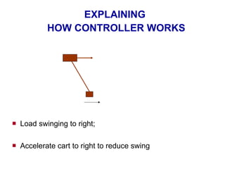
- 78. EXPLAINING HOW CONTROLLER WORKS Load swinging to right; Accelerate cart to right to reduce swing
- 79. EMPIRICAL EVALUATION Compare errors of base-learners and corresponding Q 2 learners differences btw. a base-learner and a Q 2 learner are only due to the induced qualitative constraints Experiments with three base-learners: Locally Weighted Regression (LWR) Model trees Regression trees
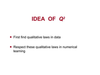
- 80. Robot Arm Domain Y 1 Y 2 Two-link, two-joint robot arm Link 1 extendible: L 1 [2, 10] Y 1 = L 1 sin( 1 ) Y 2 = L 1 sin( 1 ) + 5 sin( 1 + 2 ) 1 2 Four learning problems: A: Y 1 = f(L 1 , 1 ) B: Y 2 = f(L 1 , 1 , 2 , sum , Y 1 ) C: Y 2 = f(L 1 , 1 , 2 , sum ) D: Y 2 = f(L 1 , 1 , 2 ) L 1 Derived attribute sum = 1 + 2 Difficulty for Q 2
- 81. Robot Arm: LWR and Q 2 at different noise levels Q 2 outperforms LWR with all four learning problems (at all three noise levels) A 0, 5, 10% n. | B 0, 5, 10% n. | C 0, 5, 10% n. | D 0, 5, 10% n.
- 82. UCI and Dynamic Domains Five smallest regression data sets from UCI Dynamic domains: typical domains where QUIN was applied so far to explain the control skill or control the system until now was not possible to measure accuracy of the learned concepts (qualitative trees) AntiSway logged data from an anti-sway crane controller CraneSkill1, CraneSkill2: logged data of experienced human operators controlling a crane
- 83. UCI and Dynamic Domains: LWR compared to Q 2 Similar results with other two base-learners. Q 2 significantly better than base-learners in 18 out of 24 comparisons (24 = 8 datasets * 3 base-learners)
- 84. Q 2 - CONCLUSIONS A novel approach to numerical learning Can take into account qualitative prior knowledge Advantages: qualitative consistency of induced models and data – important for interpretation of induced models improved numerical accuracy of predictions
- 85. Q 2 TEAM + ACKNOWLEDGEMENTS Q 2 learning, QUIN, Qfilter , QCGRID (AI Lab, Ljubljana): Dorian Š uc Daniel Vladušič Car modelling data Wolfgan Rulka (INTEC, Munich) Zbinek Šika (Czech Technical Univ.) Population dynamics data Sašo Džeroski, Ljupčo Todorovski (J. Stefan Institute, Ljubljana) Lake Glumsoe Sven Joergensen Boris Kompare, Jure Žabkar, D. Vladušič
- 86. RELEVANT PAPERS Clark and Matwin 93: also used qualitative constraints in numerical predictions Š uc, Vladu š i č and Bratko; IJCAI’03 Š uc, Vladu š i č and Bratko; Artificial Intelligence Journal, 2004 Š uc and Bratko; ECML’03 Š uc and Bratko; IJCAI’05
Editor's Notes
- #36: I’ll give an example of the learning problem for QUIN algorithm. The red points on the picture are example points for the fn. z=… And this are noisy example – QUIN has to be able to learn from noisy data. We can see some qualitatively similar regions: there are 4 qual. different regions. This examples are the learning examples for QUIN: Z is the class var., and x and y are the attributes.
- #37: I’ll give an example of the learning problem for QUIN algorithm. The red points on the picture are example points for the fn. z=… And this are noisy example – QUIN has to be able to learn from noisy data. We can see some qualitatively similar regions: there are 4 qual. different regions. This examples are the learning examples for QUIN: Z is the class var., and x and y are the attributes.
- #38: From this learning examples, QUIN induces the following qual.tree that defines the partition of the attribute space into the areas with common behaviour of the class variable. In the leaves are QCFs. For example, the rightmost leaf that applies when x and y are both positive says that z is ... We say that z is …
- #39: A basic alg. for learning of q.trees uses MDL to learn …QCF, that is QCF that fits the examples best. To learn a qual. tree. a top-down greedy alg., that is similar to dec.tree learning algorithms, is used:… QUIN is heuristic improvement of this basic algorithm that considers also the consistency and prox…
- #55: Given results for ZooChange are multiplied by 1000 (actual values are 1000 times smaller)
- #64: The improvements of Q2 are even more obvious on INTEC wheel model. The blue line denotes the time behavior of toe angle alpha on the most difficult test trace.
- #65: The red line is alpha predicted by LWR.
- #66: and the orange line, alpha predicted by M5.
- #67: The green line corresponds to Q2 prediction learned from the same data. Q2 clearly has the best numerical fit. Also with other state-of-the-art numerical predictors qualitative errors are clearly visible.
- #80: To evaluate accuracy benefits of Q2 learning we compared Because Qfilter optimaly adjusts a base-learner’s predictions to be consistent with a qualitative tree, the differences… We experimented with 3 base-learners: {it RRE} is the root mean squared error normalized by the root mean squared error of average class value. Using our implementation of model and regression trees.
- #83: Now I wll describe the experiments with 5 UCI and 3 Dyanmic Domains We used the 5 smallest data sets from the UCI repository with the majority of continuous attributes. A reason for choosing these data sets is also that Quinlan gives results of M5 and several other regression methods on these data sets, which enables a better comparison of $Q^2$ to other methods. The other three data sets are from dynamic domains where QUIN has typically been previously applied to explain the underlying control skill and to use the induced qualitative models to control a dynamic system. Until now, it was not possible to measure the numerical accuracy of the learned qualitative trees or compare it to other learning methods. Data set {em AntiSway} was used in reverse-engineering of an industrial gantry crane controller. This so-called {em anti-sway crane} is used in metallurgical companies to reduce the swing of the load and increase the productivity of transportation of slabs. Data sets {em CraneSkill1} and {em CraneSkill2} are the logged data of two experienced human operators controlling a crane simulator. Such control traces are typically used to reconstruct the underlying operator's control skill. The learning task is to predict the velocity of a crane trolley given the position of the trolley, rope angle and its velocity.
- #84: The graph gives the RREs of LWR and Q2 in these 8 datasets using 10CV. Q 2 is much better in all domains, except in AutoMPG domain.