

![ND Arrays by Numpy
>>> import numpy as np
>>> x = np.array([10, 20, 30])
>>> 10 in x
True
>>> 11 in x
False
3
Abhijit Kar Gupta,
email: kg.abhi@gmail.com](https://image.slidesharecdn.com/akg-python-talk-numpy-pandas-190703192842/85/Python-for-Data-Science-and-Scientific-Computing-3-320.jpg)
![Attributes: Type, Size, Dimension
>>> x = np.array([10, 20, 30])
>>> type(x)
<type 'numpy.ndarray'>
>>> x.size
3
>>> x.dtype
dtype('int32')
>>> x.ndim
1
4
Abhijit Kar Gupta,
email: kg.abhi@gmail.com](https://image.slidesharecdn.com/akg-python-talk-numpy-pandas-190703192842/85/Python-for-Data-Science-and-Scientific-Computing-4-320.jpg)
![>>> y = np.array([[1,2,3],[4,5,6]])
>>> y
array([[1, 2, 3],
[4, 5, 6]])
>>> y.ndim
2
>>> y.size
6
5
Abhijit Kar Gupta,
email: kg.abhi@gmail.com](https://image.slidesharecdn.com/akg-python-talk-numpy-pandas-190703192842/85/Python-for-Data-Science-and-Scientific-Computing-5-320.jpg)
![>>> M = np.array([[[1,2],[3,4]], [[5,6],[7,8]]])
>>> M
array([[[1, 2],
[3, 4]],
[[5, 6],
[7, 8]]])
>>> M.ndim
3
6
Abhijit Kar Gupta,
email: kg.abhi@gmail.com](https://image.slidesharecdn.com/akg-python-talk-numpy-pandas-190703192842/85/Python-for-Data-Science-and-Scientific-Computing-6-320.jpg)

![Default Data type
>>> x = np.array([10, 23, 36, 467])
>>> x.dtype
dtype('int32')
>>> y = np.array([10.5, 23, 36, 467])
>>> y.dtype
dtype('float64')
>>> a = np.array(['ab','bc', 'ca', 100])
>>> a
array(['ab', 'bc', 'ca', '100'], dtype='|S3')
*S3 = String of length 3.
8
Abhijit Kar Gupta,
email: kg.abhi@gmail.com](https://image.slidesharecdn.com/akg-python-talk-numpy-pandas-190703192842/85/Python-for-Data-Science-and-Scientific-Computing-8-320.jpg)
![Given Data type
>>> x = np.array([10,20,30], dtype = 'f')
>>> x
array([10., 20., 30.], dtype = float32)
>>> x = np.array([10.5,23,36,467], dtype = 'f4')
>>> x
array([ 10.5, 23. , 36. , 467. ], dtype = float32)
>>> x = np.array([10.5,23,36,467], dtype = 'complex')
>>> x
array([ 10.5+0.j, 23. +0.j, 36. +0.j, 467. +0.j])
>>> x.dtype
dtype('complex128')
>>> x = np.array([10.5,23,36,467], dtype = 'complex64')
>>> x.dtype
dtype('complex64')
9
Abhijit Kar Gupta,
email: kg.abhi@gmail.com](https://image.slidesharecdn.com/akg-python-talk-numpy-pandas-190703192842/85/Python-for-Data-Science-and-Scientific-Computing-9-320.jpg)
![>>> A = np.array(['ab', 'bc', 'ca', 100], dtype = 'S10')
>>> A
array(['ab', 'bc', 'ca', '100'], dtype='|S10')
>>> A = np.array(['ab','bc', 'ca', 'abracadabra',
100], dtype = 'S6')
>>> A
array(['ab', 'bc', 'ca', 'abraca', '100'], dtype=
'|S6')
>>> A.itemsize # Size of each item
6
10
Abhijit Kar Gupta,
email: kg.abhi@gmail.com](https://image.slidesharecdn.com/akg-python-talk-numpy-pandas-190703192842/85/Python-for-Data-Science-and-Scientific-Computing-10-320.jpg)
![Methods for creation of arrays
np.arange(start, stop, step)
>>> np.arange(3)
array([0, 1, 2])
>>> np.arange(3.0)
array([0., 1., 2.])
>>> np.arange(3, 15, 2, dtype ='float')
array([ 3., 5., 7., 9., 11., 13.])
>>> np.arange(0.5, 1.0, 0.1)
array([0.5, 0.6, 0.7, 0.8, 0.9])
11
Abhijit Kar Gupta,
email: kg.abhi@gmail.com](https://image.slidesharecdn.com/akg-python-talk-numpy-pandas-190703192842/85/Python-for-Data-Science-and-Scientific-Computing-11-320.jpg)
![np.linspace(start, end, num)
>>> np.linspace(10, 20, 5)
array([10. , 12.5, 15. , 17.5, 20. ])
>>> np.linspace(10, 20, 5, endpoint = True)
array([10. , 12.5, 15. , 17.5, 20. ])
>>> np.linspace(10, 20, 5, endpoint = False)
array([10., 12., 14., 16., 18.])
>>> np.linspace(10, 20, 5, retstep = True)
(array([10. , 12.5, 15. , 17.5, 20. ]), 2.5)
# returns step value
12
Abhijit Kar Gupta,
email: kg.abhi@gmail.com](https://image.slidesharecdn.com/akg-python-talk-numpy-pandas-190703192842/85/Python-for-Data-Science-and-Scientific-Computing-12-320.jpg)
![# Evenly spaced in logscale
>>> np.logspace(0, 1, 10)
array([ 1., 1.29154967, 1.66810054, 2.15443469,
2.7825594,3.59381366, 4.64158883, 5.9948425,
7.74263683, 10.])
# 10 vales, default base = 10
>>> x = np.logspace(0, 1, 10)
>>> np.log10(x)
array([0., 0.11111111, 0.22222222, 0.33333333,
0.44444444, 0.55555556, 0.66666667, 0.77777778,
0.88888889, 1.])
>>> np.logspace(0, 1, 10, base = 2)
array([1., 1.08005974, 1.16652904, 1.25992105,
1.36079,1.46973449, 1.58740105, 1.71448797,
1.85174942, 2.])
13
Abhijit Kar Gupta,
email: kg.abhi@gmail.com](https://image.slidesharecdn.com/akg-python-talk-numpy-pandas-190703192842/85/Python-for-Data-Science-and-Scientific-Computing-13-320.jpg)
![Shape/Reshape
>>> a = np.arange(0,60,5)
>>> a
array([ 0, 5, 10, 15, 20, 25, 30, 35, 40, 45, 50, 55])
>>> np.shape(a)
(12,)
>>> a.shape
(12,)
>>> np.reshape(a, (3,4))
array([[ 0, 5, 10, 15],
[20, 25, 30, 35],
[40, 45, 50, 55]])
>>> b = a.reshape(3,4)
>>> np.shape(b)
(3, 4)
>>> b.shape
(3, 4)
14
Abhijit Kar Gupta,
email: kg.abhi@gmail.com](https://image.slidesharecdn.com/akg-python-talk-numpy-pandas-190703192842/85/Python-for-Data-Science-and-Scientific-Computing-14-320.jpg)
![Unique elements
>>> y = np.array([1,2,1,0.5,10,2,10])
>>> np.unique(y)
array([ 0.5, 1. , 2. , 10. ])
>>> L = np.random.randint(0, 2, (4,5))
>>> L
array([[0, 1, 0, 0, 0],
[0, 1, 1, 1, 0],
[1, 0, 1, 0, 0],
[0, 1, 0, 1, 1]])
>>> np.unique(L)
array([0, 1])
>>> A = np.array(['a', 'b', 'c', 'a', 'b', 'a'])
>>> np.unique(A)
array(['a', 'b', 'c'], dtype='|S1')
15
Abhijit Kar Gupta,
email: kg.abhi@gmail.com](https://image.slidesharecdn.com/akg-python-talk-numpy-pandas-190703192842/85/Python-for-Data-Science-and-Scientific-Computing-15-320.jpg)
![Iterator
>>> import numpy as np
>>> x = np.array([10, 20, 30, 40])
>>> for i in x:
print i
10
20
30
40
>>> A = np.arange(0,60,5).reshape(3, 4)
>>> for i in A:
print i
[ 0 5 10 15]
[20 25 30 35]
[40 45 50 55]
16
Abhijit Kar Gupta,
email: kg.abhi@gmail.com](https://image.slidesharecdn.com/akg-python-talk-numpy-pandas-190703192842/85/Python-for-Data-Science-and-Scientific-Computing-16-320.jpg)


![Inserting Elements
>>> a = np.array([0, -1, 2, 5, 10])
>>> a.put(3, 99)
>>> a
array([ 0, -1, 2, 99, 10])
>>> np.insert(a, 3, 99)
array([ 0, -1, 2, 99, 5, 10])
19
Abhijit Kar Gupta,
email: kg.abhi@gmail.com](https://image.slidesharecdn.com/akg-python-talk-numpy-pandas-190703192842/85/Python-for-Data-Science-and-Scientific-Computing-19-320.jpg)
![>>> A = np.array([[1,2], [3,4]])
>>> A
array([[1, 2],
[3, 4]])
>>> np.insert(A, 1, [10, 12], axis = 0)
array([[ 1, 2],
[10, 12],
[ 3, 4]])
>>> np.insert(A, 1, [10, 12], axis = 1)
array([[ 1, 10, 2],
[ 3, 12, 4]])
20
Abhijit Kar Gupta,
email: kg.abhi@gmail.com](https://image.slidesharecdn.com/akg-python-talk-numpy-pandas-190703192842/85/Python-for-Data-Science-and-Scientific-Computing-20-320.jpg)
![>>> np.insert(A, 1, [10, 12])
array([ 1, 10, 12, 2, 3, 4])
# Flattened when without axis ref
>>> np.insert(A, 1, [10])
array([ 1, 10, 2, 3, 4])
>>> np.insert(A, 1, [10], axis = 0)
array([[ 1, 2],
[10, 10],
[ 3, 4]])
>>> np.insert(A, 1, [10], axis = 1)
array([[ 1, 10, 2],
[ 3, 10, 4]])
>>> np.insert(A, 1, [10,12], axis = 0)
array([[ 1, 2],
[10, 12],
[ 3, 4]])
21
Abhijit Kar Gupta,
email: kg.abhi@gmail.com](https://image.slidesharecdn.com/akg-python-talk-numpy-pandas-190703192842/85/Python-for-Data-Science-and-Scientific-Computing-21-320.jpg)
![Deleting
>>> x = np.arange(1, 13).reshape(3,4)
>>> x
array([[ 1, 2, 3, 4],
[ 5, 6, 7, 8],
[ 9, 10, 11, 12]])
>>> np.delete(x, 2, axis = 0)
array([[1, 2, 3, 4],
[5, 6, 7, 8]])
>>> np.delete(x, 2, axis = 1)
array([[ 1, 2, 4],
[ 5, 6, 8],
[ 9, 10, 12]])
22
Abhijit Kar Gupta,
email: kg.abhi@gmail.com](https://image.slidesharecdn.com/akg-python-talk-numpy-pandas-190703192842/85/Python-for-Data-Science-and-Scientific-Computing-22-320.jpg)
![Split
>>> np.split(x, 3)
[array([[1, 2, 3, 4]]), array([[5, 6, 7, 8]]), array([[ 9,
10, 11, 12]])]
>>> np.vsplit(x, 3)
# same as above (row wise split)
>>> np.hsplit(x, 4)
[array([[1],
[5],
[9]]),
array([[ 2],
[ 6],
[10]]),
array([[ 3],
[ 7],
[11]]),
array([[ 4],
[ 8],
[12]])]
23
Abhijit Kar Gupta,
email: kg.abhi@gmail.com](https://image.slidesharecdn.com/akg-python-talk-numpy-pandas-190703192842/85/Python-for-Data-Science-and-Scientific-Computing-23-320.jpg)
![Append
>>> x = np.array([1, 2, 3, 4])
>>> np.append(x, 7)
array([1, 2, 3, 4, 7])
>>> x = np.array([10, 20, 30])
>>> y = np.array([100, 200, 300])
>>> np.append(x, y)
array([ 10, 20, 30, 100, 200, 300])
24
Abhijit Kar Gupta,
email: kg.abhi@gmail.com](https://image.slidesharecdn.com/akg-python-talk-numpy-pandas-190703192842/85/Python-for-Data-Science-and-Scientific-Computing-24-320.jpg)
![>>> A = np.array([[1,2], [3,4]])
>>> A
array([[1, 2],
[3, 4]])
>>> np.append(A, 99)
array([ 1, 2, 3, 4, 99])
#flattens and appends
>>> np.append(A, [[9,10]], axis = 0)
array([[ 1, 2],
[ 3, 4],
[ 9, 10]])
25
Abhijit Kar Gupta,
email: kg.abhi@gmail.com](https://image.slidesharecdn.com/akg-python-talk-numpy-pandas-190703192842/85/Python-for-Data-Science-and-Scientific-Computing-25-320.jpg)
![Complex arrays
>>> x = np.array([2+3j, 5+2j, 3-1j])
>>> x.real
array([2., 5., 3.])
>>> x.imag
array([ 3., 2., -1.])
>>> x.conj()
array([2.-3.j, 5.-2.j, 3.+1.j])
26
Abhijit Kar Gupta,
email: kg.abhi@gmail.com](https://image.slidesharecdn.com/akg-python-talk-numpy-pandas-190703192842/85/Python-for-Data-Science-and-Scientific-Computing-26-320.jpg)
![Statistics
>>> x = np.arange(10, 100, 10)
>>> x
array([10, 20, 30, 40, 50, 60, 70, 80, 90])
>>> np.sum(x)
450
>>> np.cumsum(x)
array([ 10, 30, 60, 100, 150, 210, 280, 360, 450])
>>> x = np.arange(10, 100, 10).reshape(3,3)
>>> x
array([[10, 20, 30],
[40, 50, 60],
[70, 80, 90]])
>>> np.sum(x)
450
>>> np.sum(x, 0) # 0 axis
array([120, 150, 180])
>>> np.sum(x, 1) # 1 axis
27
Abhijit Kar Gupta,
email: kg.abhi@gmail.com](https://image.slidesharecdn.com/akg-python-talk-numpy-pandas-190703192842/85/Python-for-Data-Science-and-Scientific-Computing-27-320.jpg)
![>>> np.trace(x)
150
>>> np.trace(x, 1)
80
>>> np.trace(x, -1)
120
>>> np.mean(x)
50.0
>>> np.mean(x,1)
array([20., 50., 80.])
>>> np.mean(x,0)
array([40., 50., 60.])
>>> np.median(x)
50.0
>>> np.median(x,0)
array([40., 50., 60.])
>>> np.median(x,1)
array([20., 50., 80.])
28
Abhijit Kar Gupta,
email: kg.abhi@gmail.com](https://image.slidesharecdn.com/akg-python-talk-numpy-pandas-190703192842/85/Python-for-Data-Science-and-Scientific-Computing-28-320.jpg)
![>>> x = np.array([0, -1, 2, 5, 10, 3, -2, 4])
>>> np.ptp(x) # peak to peak
12
>>> np.var(x) # variance
12.984375
>>> np.std(x) # standard dev
3.6033838263498934
29
Abhijit Kar Gupta,
email: kg.abhi@gmail.com](https://image.slidesharecdn.com/akg-python-talk-numpy-pandas-190703192842/85/Python-for-Data-Science-and-Scientific-Computing-29-320.jpg)
![>>> x = np.array([0, -1, 2, 5, 10, 3, -2, 4]).reshape(2,4)
>>> x
array([[ 0, -1, 2, 5],
[10, 3, -2, 4]])
>>> np.ptp(x, 0)
array([10, 4, 4, 1])
>>> np.ptp(x, 1)
array([ 6, 12])
30
Abhijit Kar Gupta,
email: kg.abhi@gmail.com](https://image.slidesharecdn.com/akg-python-talk-numpy-pandas-190703192842/85/Python-for-Data-Science-and-Scientific-Computing-30-320.jpg)
![Sorting
>>> L = np.random.randint(-10, 10, (4,5))
>>> L
array([[-6, -4, -7, 5, 6],
[ 0, -9, -8, -4, -1],
[ 0, 8, -5, 0, 2],
[-8, -5, -2, -2, -8]])
>>> np.sort(L)
array([[-7, -6, -4, 5, 6],
[-9, -8, -4, -1, 0],
[-5, 0, 0, 2, 8],
[-8, -8, -5, -2, -2]])
>>> np.sort(L, 0)
array([[-8, -9, -8, -4, -8],
[-6, -5, -7, -2, -1],
[ 0, -4, -5, 0, 2],
[ 0, 8, -2, 5, 6]])
>>> np.sort(L, 1)
array([[-7, -6, -4, 5, 6],
[-9, -8, -4, -1, 0],
[-5, 0, 0, 2, 8],
[-8, -8, -5, -2, -2]])
31
Abhijit Kar Gupta,
email: kg.abhi@gmail.com](https://image.slidesharecdn.com/akg-python-talk-numpy-pandas-190703192842/85/Python-for-Data-Science-and-Scientific-Computing-31-320.jpg)
![Concatenation
>>> x = np.array([10,20,30])
>>> y = np.array([40,50,60])
>>> np.concatenate((x,y))
array([10, 20, 30, 40, 50, 60])
32
Abhijit Kar Gupta,
email: kg.abhi@gmail.com](https://image.slidesharecdn.com/akg-python-talk-numpy-pandas-190703192842/85/Python-for-Data-Science-and-Scientific-Computing-32-320.jpg)
![>>> x = np.array([[1,2,3],[4,5,6]])
>>> y = np.array([[7,8,9],[10,11,12]])
>>> np.concatenate((x,y))
array([[1, 2, 3],
[4, 5, 6],
[7, 8, 9],
[10, 11, 12]])
>>> np.concatenate((x,y), axis = 1)
array([[1, 2, 3, 7, 8, 9],
[4, 5, 6, 10, 11, 12]])
33
Abhijit Kar Gupta,
email: kg.abhi@gmail.com](https://image.slidesharecdn.com/akg-python-talk-numpy-pandas-190703192842/85/Python-for-Data-Science-and-Scientific-Computing-33-320.jpg)
![mgrid
>>> xx, yy = np.mgrid[-5:5:0.1, -5:5:0.1]
>>> x = xx[:,0]
>>> y = yy[0,:]
>>> xx
array([[-5. , -5. , -5. , ..., -5. , -5. , -5. ],
[-4.9, -4.9, -4.9, ..., -4.9, -4.9, -4.9],
[-4.8, -4.8, -4.8, ..., -4.8, -4.8, -4.8],
...,
[ 4.7, 4.7, 4.7, ..., 4.7, 4.7, 4.7],
[ 4.8, 4.8, 4.8, ..., 4.8, 4.8, 4.8],
[ 4.9, 4.9, 4.9, ..., 4.9, 4.9, 4.9]])
>>> yy
array([[-5. , -4.9, -4.8, ..., 4.7, 4.8, 4.9],
[-5. , -4.9, -4.8, ..., 4.7, 4.8, 4.9],
[-5. , -4.9, -4.8, ..., 4.7, 4.8, 4.9],
...,
[-5. , -4.9, -4.8, ..., 4.7, 4.8, 4.9],
[-5. , -4.9, -4.8, ..., 4.7, 4.8, 4.9],
[-5. , -4.9, -4.8, ..., 4.7, 4.8, 4.9]])
35
Abhijit Kar Gupta,
email: kg.abhi@gmail.com](https://image.slidesharecdn.com/akg-python-talk-numpy-pandas-190703192842/85/Python-for-Data-Science-and-Scientific-Computing-35-320.jpg)

![Special arrays
>>> np.eye(3)
array([[1., 0., 0.],
[0., 1., 0.],
[0., 0., 1.]])
>>> np.zeros(3)
array([0., 0., 0.])
>>> np.zeros((3,3))
array([[0., 0., 0.],
[0., 0., 0.],
[0., 0., 0.]])
>>> np.full((3,3),5)
array([[5, 5, 5],
[5, 5, 5],
[5, 5, 5]])
37
Abhijit Kar Gupta,
email: kg.abhi@gmail.com](https://image.slidesharecdn.com/akg-python-talk-numpy-pandas-190703192842/85/Python-for-Data-Science-and-Scientific-Computing-37-320.jpg)
![>>> a = np.array([[1,2],[3,4]])
>>> a
array([[1, 2],
[3, 4]])
>>> np.zeros_like(a)
array([[0, 0],
[0, 0]])
>>> np.diag((1,2,3))
array([[1, 0, 0],
[0, 2, 0],
[0, 0, 3]])
>>> np.diag((1,2,3), k = 1)
array([[0, 1, 0, 0],
[0, 0, 2, 0],
[0, 0, 0, 3],
[0, 0, 0, 0]])
38
Abhijit Kar Gupta,
email: kg.abhi@gmail.com](https://image.slidesharecdn.com/akg-python-talk-numpy-pandas-190703192842/85/Python-for-Data-Science-and-Scientific-Computing-38-320.jpg)
![Indexing, Slicing
>>> x = np.arange(2, 15, 3)
>>> x
array([2, 5, 8, 11, 14])
>>> x[0]
2
>>> x[2]
8
>>> x[-1]
14
>>> x[1:5:2]
array([5, 11])
Also, one can write: s = slice(1,5,2) and then x[s]
39
Abhijit Kar Gupta,
email: kg.abhi@gmail.com](https://image.slidesharecdn.com/akg-python-talk-numpy-pandas-190703192842/85/Python-for-Data-Science-and-Scientific-Computing-39-320.jpg)
![>>> x[3:]
array([11, 14])
>>> x[:4]
array([ 2, 5, 8, 11])
>>> x[::2]
array([ 2, 8, 14])
>>> x[2::]
array([ 8, 11, 14])
>>> x[::-1]
array([14, 11, 8, 5, 2])
>>> x[::-3]
array([14, 5])
40
Abhijit Kar Gupta,
email: kg.abhi@gmail.com](https://image.slidesharecdn.com/akg-python-talk-numpy-pandas-190703192842/85/Python-for-Data-Science-and-Scientific-Computing-40-320.jpg)
![>>> x = np.arange(12).reshape(4,3)
>>> x
array([[ 0, 1, 2],
[ 3, 4, 5],
[ 6, 7, 8],
[ 9, 10, 11]])
>>> x[2:]
array([[ 6, 7, 8],
[ 9, 10, 11]])
>>> x[:3]
array([[0, 1, 2],
[3, 4, 5],
[6, 7, 8]])
>>> x[::2]
array([[0, 1, 2],
[6, 7, 8]])
41
Abhijit Kar Gupta,
email: kg.abhi@gmail.com](https://image.slidesharecdn.com/akg-python-talk-numpy-pandas-190703192842/85/Python-for-Data-Science-and-Scientific-Computing-41-320.jpg)
![>>> x[:]
array([[ 0, 1, 2, 3],
[ 4, 5, 6, 7],
[ 8, 9, 10, 11]])
>>> x[:,0]
array([0, 4, 8])
>>> x[:,1:3]
array([[ 1, 2],
[ 5, 6],
[ 9, 10]])
>>> x[1:3, 1:3]
array([[ 5, 6],
[ 9, 10]])
42
Abhijit Kar Gupta,
email: kg.abhi@gmail.com](https://image.slidesharecdn.com/akg-python-talk-numpy-pandas-190703192842/85/Python-for-Data-Science-and-Scientific-Computing-42-320.jpg)
![>>> x[x > 3]
array([ 4, 5, 6, 7, 8, 9, 10, 11])
# returns the elements in 1D array
>>> x.flatten()
array([ 0, 1, 2, 3, 4, 5, 6, 7, 8,
9, 10, 11])
>>> x.flatten(0)
array([ 0, 1, 2, 3, 4, 5, 6, 7, 8,
9, 10, 11])
>>> x.flatten(1)
array([ 0, 3, 6, 9, 1, 4, 7, 10, 2,
5, 8, 11])
43
Abhijit Kar Gupta,
email: kg.abhi@gmail.com](https://image.slidesharecdn.com/akg-python-talk-numpy-pandas-190703192842/85/Python-for-Data-Science-and-Scientific-Computing-43-320.jpg)
![Arithmetic Operations
>>> x = np.array([1, 2, 3, 4])
>>> y = np.array([5, 6, 7, 8])
>>> x*y
array([ 5, 12, 21, 32])
>>> x+y
array([ 6, 8, 10, 12])
>>> x-y
array([-4, -4, -4, -4])
>>> x/y
array([0, 0, 0, 0])
>>> x**y
array([ 1, 64, 2187, 65536])
44
Abhijit Kar Gupta,
email: kg.abhi@gmail.com](https://image.slidesharecdn.com/akg-python-talk-numpy-pandas-190703192842/85/Python-for-Data-Science-and-Scientific-Computing-44-320.jpg)
![>>> x = np.arange(1,7).reshape(2,3)
>>> x
array([[1, 2, 3],
[4, 5, 6]])
>>> y = np.array([10, 11, 12])
>>> x + y
array([[11, 13, 15],
[14, 16, 18]])
>>> x + 2
array([[3, 4, 5],
[6, 7, 8]])
>>> x + [2, 3, 4]
array([[ 3, 5, 7],
[ 6, 8, 10]])
* Broadcasting!
45
Abhijit Kar Gupta,
email: kg.abhi@gmail.com](https://image.slidesharecdn.com/akg-python-talk-numpy-pandas-190703192842/85/Python-for-Data-Science-and-Scientific-Computing-45-320.jpg)
![Array manipulation
>>> x
array([[1, 2, 3],
[4, 5, 6]])
>>> x.T
array([[1, 4],
[2, 5],
[3, 6]])
>>> x.transpose()
array([[1, 4],
[2, 5],
[3, 6]])
46
Abhijit Kar Gupta,
email: kg.abhi@gmail.com](https://image.slidesharecdn.com/akg-python-talk-numpy-pandas-190703192842/85/Python-for-Data-Science-and-Scientific-Computing-46-320.jpg)
![Stacking
>>> x
array([[1, 2],
[3, 4]])
>>> y
array([[5, 6],
[7, 8]])
>>> np.stack((x,y)) # default axis = 0
array([[[1, 2],
[3, 4]],
[[5, 6],
[7, 8]]])
>>> np.stack((x,y),axis = 1)
array([[[1, 2],
[5, 6]],
[[3, 4],
[7, 8]]])
47
Abhijit Kar Gupta,
email: kg.abhi@gmail.com](https://image.slidesharecdn.com/akg-python-talk-numpy-pandas-190703192842/85/Python-for-Data-Science-and-Scientific-Computing-47-320.jpg)
![>>> np.vstack((x, y)) # stacks vertically
array([[1, 2],
[3, 4],
[5, 6],
[7, 8]])
>>> np.hstack((x, y)) # stacks horizontally
array([[1, 2, 5, 6],
[3, 4, 7, 8]])
48
Abhijit Kar Gupta,
email: kg.abhi@gmail.com](https://image.slidesharecdn.com/akg-python-talk-numpy-pandas-190703192842/85/Python-for-Data-Science-and-Scientific-Computing-48-320.jpg)
![Numpy Functions
Functions over arrays
>>> import numpy as np
>>> x = np.arange(0, 1, 0.1)
>>> x
array([0. , 0.1, 0.2, 0.3, 0.4, 0.5, 0.6, 0.7, 0.8,
0.9])
>>> np.sin(x)
array([0., 0.09983342, 0.19866933, 0.29552021,
0.38941834, 0.47942554, 0.56464247, 0.64421769,
0.71735609, 0.78332691])
>>> f = lambda x: x**2
>>> f(x)
array([0., 0.01, 0.04, 0.09, 0.16, 0.25, 0.36, 0.49,
0.64, 0.81])
49
Abhijit Kar Gupta,
email: kg.abhi@gmail.com](https://image.slidesharecdn.com/akg-python-talk-numpy-pandas-190703192842/85/Python-for-Data-Science-and-Scientific-Computing-49-320.jpg)
![>>> x = range(1, 5)
>>> x
[1, 2, 3, 4]
>>> np.sqrt(x)
array([1., 1.41421356, 1.73205081, 2. ])
>>> f = lambda x: x**2
>>> f(x)
Traceback (most recent call last):
File "<pyshell#85>", line 1, in <module>
f(x)
File "<pyshell#84>", line 1, in <lambda>
f = lambda x: x**2
TypeError: unsupported operand type(s) for ** or
pow(): 'list' and 'int'
50
Abhijit Kar Gupta,
email: kg.abhi@gmail.com](https://image.slidesharecdn.com/akg-python-talk-numpy-pandas-190703192842/85/Python-for-Data-Science-and-Scientific-Computing-50-320.jpg)
![Vectorize
>>> f1 = np.vectorize(f)
>>> type(f1)
<class 'numpy.vectorize'>
>>> f1(x)
array([ 1, 4, 9, 16])
51
Abhijit Kar Gupta,
email: kg.abhi@gmail.com](https://image.slidesharecdn.com/akg-python-talk-numpy-pandas-190703192842/85/Python-for-Data-Science-and-Scientific-Computing-51-320.jpg)
![Arrays as Vectors
# Inner Product
>>> u = np.array([1,2,3])
>>> v = np.array([-1,0,1])
>>> np.inner(u,v)
2
>>> np.inner(u, 2)
array([2, 4, 6])
>>> np.inner(np.eye(3),5))
array([[5., 0., 0.],
[0., 5., 0.],
[0., 0., 5.]])
52
Abhijit Kar Gupta,
email: kg.abhi@gmail.com](https://image.slidesharecdn.com/akg-python-talk-numpy-pandas-190703192842/85/Python-for-Data-Science-and-Scientific-Computing-52-320.jpg)
![# Multidimensional inner product
>>> A = np.array([[1,2,3],[4,5,6]])
>>> B = np.array([[1,0,1],[0,1,0]])
>>> np.inner(A,B)
array([[ 4, 2],
[10, 5]])
53
Abhijit Kar Gupta,
email: kg.abhi@gmail.com](https://image.slidesharecdn.com/akg-python-talk-numpy-pandas-190703192842/85/Python-for-Data-Science-and-Scientific-Computing-53-320.jpg)
![>>> data = np.genfromtxt('test.dat')
>>> data
array([[ 1. , 100. , 1.1, -6.1, -5.1, -6.1],
[ 2. , 200. , 1.2, -15.4, -15.4, -15.4],
[ 3. , 300. , 1.3, -15. , -15. , -15. ],
[ 4. , 400. , 1.4, -19.3, -19.3, -19.3],
[ 5. , 500. , 1.5, -16.8, -16.8, -16.8],
[ 6. , 600. , 1.6, -11.4, -11.4, -11.4],
[ 7. , 700. , 1.7, -7.6, -7.6, -7.6],
[ 8. , 800. , 1.8, -7.1, -7.1, -7.1],
[ 9. , 900. , 1.9, -10.1, -10.1, -10.1],
[ 10. , 1000. , 2. , 10. , -9.5, -9.5]])
>>> data = np.loadtxt('test.dat')
>>> R = np.random.randint(1, 10, (3,4))
>>> R
array([[7, 5, 1, 2],
[8, 4, 9, 4],
[9, 4, 6, 7]])
>>> np.savetxt('random.dat', R)
55
Abhijit Kar Gupta,
email: kg.abhi@gmail.com](https://image.slidesharecdn.com/akg-python-talk-numpy-pandas-190703192842/85/Python-for-Data-Science-and-Scientific-Computing-55-320.jpg)
![# Vector Cross Product
>>> x = np.array([1, 2, 3])
>>> y = np.array([-1,3, 0])
>>> np.cross(x, y)
array([-9, -3, 5])
Volume of a Parallelepiped:
Three sides are given by three vectors: 𝑨 = 𝟐𝒊 − 𝟑𝒋, 𝑩 = 𝒊 + 𝒋 − 𝒌,
𝑪 = 𝟑𝒊 − 𝒌
Volume = 𝑨. 𝑩 × 𝑪 = 𝟒
>>> a = np.array([2, -3, 0])
>>> b = np.array([1, 1, -1])
>>> c = np.array([3, 0, -1])
>>> np.vdot(a, np.cross(b, c))
4
56
Abhijit Kar Gupta,
email: kg.abhi@gmail.com](https://image.slidesharecdn.com/akg-python-talk-numpy-pandas-190703192842/85/Python-for-Data-Science-and-Scientific-Computing-56-320.jpg)
![Matrix Like Operations
>>> A = np.array([[1,2,3],[4,5,6]])
>>> B = np.array([[1,2],[3,4],[5,6]])
>>> np.dot(A,B)
array([[22, 28],
[49, 64]])
>>> A.dot(B)
array([[22, 28],
[49, 64]])
>>> B.dot(A)
array([[ 9, 12, 15],
[19, 26, 33],
[29, 40, 51]])
AB ≠ BA
57
Abhijit Kar Gupta,
email: kg.abhi@gmail.com](https://image.slidesharecdn.com/akg-python-talk-numpy-pandas-190703192842/85/Python-for-Data-Science-and-Scientific-Computing-57-320.jpg)
![Matrix
>>> X = np.matrix(A)
>>> Y = np.matrix(B)
>>> X*Y
matrix([[22, 28],
[49, 64]])
>>> Y*X
matrix([[ 9, 12, 15],
[19, 26, 33],
[29, 40, 51]])
58
Abhijit Kar Gupta,
email: kg.abhi@gmail.com](https://image.slidesharecdn.com/akg-python-talk-numpy-pandas-190703192842/85/Python-for-Data-Science-and-Scientific-Computing-58-320.jpg)
![Complex Matrix
>>> C = np.matrix([[1+2j, 1j], [2-3j, 4j]])
>>> C
matrix([[1.+2.j, 0.+1.j],
[2.-3.j, 0.+4.j]])
>>> C.T
matrix([[1.+2.j, 2.-3.j],
[0.+1.j, 0.+4.j]])
>>> C.conjugate()
matrix([[1.-2.j, 0.-1.j],
[2.+3.j, 0.-4.j]])
>>> np.angle(C)
matrix([[ 1.10714872, 1.57079633],
[-0.98279372, 1.57079633]])
>>> C.H #Adjoint Matrix
matrix([[1.-2.j, 2.+3.j],
[0.-1.j, 0.-4.j]])
59
Abhijit Kar Gupta,
email: kg.abhi@gmail.com](https://image.slidesharecdn.com/akg-python-talk-numpy-pandas-190703192842/85/Python-for-Data-Science-and-Scientific-Computing-59-320.jpg)
![Eigen values, Eigen vectors
>>> import numpy as np
>>> import numpy.linalg as lin
>>> A = np.array([[1,2],[3,4]])
>>> lin.eig(A)
(array([-0.37228132, 5.37228132]),
array([[-0.82456484, -0.41597356],[
0.56576746, -0.90937671]]))
>>> eigen_val, eigen_vec = lin.eig(A)
60
Abhijit Kar Gupta,
email: kg.abhi@gmail.com](https://image.slidesharecdn.com/akg-python-talk-numpy-pandas-190703192842/85/Python-for-Data-Science-and-Scientific-Computing-60-320.jpg)
![>>> eigen_val
array([-0.37228132, 5.37228132])
>>> eigen_vec
array([[-0.82456484, -0.41597356],
[ 0.56576746, -0.90937671]])
>>> eigen_vec[:,0]
array([-0.82456484, 0.56576746])
>>> eigen_vec[:,1]
array([-0.41597356, -0.90937671])
61
Abhijit Kar Gupta,
email: kg.abhi@gmail.com](https://image.slidesharecdn.com/akg-python-talk-numpy-pandas-190703192842/85/Python-for-Data-Science-and-Scientific-Computing-61-320.jpg)
![Linear Algebra
𝑥1 + 2𝑥2 − 𝑥3 = 1
2𝑥1 + 𝑥2 +4𝑥3 = 2
3𝑥1 + 3𝑥2 + 4𝑥3 = 1
A =
1 2 −1
2 1 4
3 3 4
, x =
𝑥1
𝑥2
𝑥3
, and b =
1
2
1
>>> import numpy as np
>>> a = np.array([[1,2,-1],[2,1,4],[3,3,4]])
>>> b = np.array([1,2,1])
>>> print np.linalg.solve(a,b)
[ 7. -4. -2.]
62
Abhijit Kar Gupta,
email: kg.abhi@gmail.com](https://image.slidesharecdn.com/akg-python-talk-numpy-pandas-190703192842/85/Python-for-Data-Science-and-Scientific-Computing-62-320.jpg)
![Matrix Inverse
>>> import numpy as np
>>> A = np.array([[1,1,1], [1,2,3], [1,4,9]])
>>> Ainv = np.linalg.inv(A)
>>> Ainv
array([[ 3. , -2.5, 0.5],
[-3. , 4. , -1. ],
[ 1. , -1.5, 0.5]])
63
Abhijit Kar Gupta,
email: kg.abhi@gmail.com](https://image.slidesharecdn.com/akg-python-talk-numpy-pandas-190703192842/85/Python-for-Data-Science-and-Scientific-Computing-63-320.jpg)
![Polynomial by Numpy
>>> from numpy import poly1d
>>> p = np.poly1d([1,2,3])
>>> print p
1 𝑥2
+ 2 𝑥 + 3
>>> p(2)
11
>>> p(-1)
2
>>> p.c # Coefficients
array([1, 2, 3])
>>> p.order # Order of the polynomial
2
64
Abhijit Kar Gupta,
email: kg.abhi@gmail.com](https://image.slidesharecdn.com/akg-python-talk-numpy-pandas-190703192842/85/Python-for-Data-Science-and-Scientific-Computing-64-320.jpg)
![Methods on Polynomials
>>> from numpy import poly1d as poly
>>> p1 = poly([1,5,6])
>>> p2 = poly([1,2])
>>> p1 + p2
poly1d([1, 6, 8])
>>> p1*p2
poly1d([ 1, 7, 16, 12])
>>> p1/p2
(poly1d([1., 3.]), poly1d([0.]))
>>> p2**2
poly1d([1, 4, 4])
>>> from numpy import sin
>>> sin(p2)
array([0.84147098, 0.90929743])
65
Abhijit Kar Gupta,
email: kg.abhi@gmail.com](https://image.slidesharecdn.com/akg-python-talk-numpy-pandas-190703192842/85/Python-for-Data-Science-and-Scientific-Computing-65-320.jpg)
![>>> p = np.poly1d([1, -5, 6])
>>> p.r
array([3., 2.]) # Real roots: 3, 2
>>> p.deriv(1) # First derivative
poly1d([2, 2])
>>> p.deriv(2) # Second derivative
poly1d([2])
>>> p.integ(1)
poly1d([0.33333333, 1. , 3. , 0. ])
>>> p.integ(2)
poly1d([0.08333333, 0.33333333,1.5,0.,0. ])
66
Abhijit Kar Gupta,
email: kg.abhi@gmail.com](https://image.slidesharecdn.com/akg-python-talk-numpy-pandas-190703192842/85/Python-for-Data-Science-and-Scientific-Computing-66-320.jpg)
![Plotting by Matplotlib
>>> import matplotlib.pyplot as plt
>>> x = [1, 2, 3, 4, 5]
>>> y = [1, 4, 9, 16, 25]
>>> plt.plot(x, y)
[<matplotlib.lines.Line2D object at
0x000000000BE00B70>]
>>> plt.show()
67
Abhijit Kar Gupta,
email: kg.abhi@gmail.com](https://image.slidesharecdn.com/akg-python-talk-numpy-pandas-190703192842/85/Python-for-Data-Science-and-Scientific-Computing-67-320.jpg)
![To plot the polynomial and
see…
68
>>> import numpy as np
>>> import matplotlib.pyplot as plt
>>> x = np.linspace(-10,10,100)
>>> p = np.poly1d([1, 2, -3])
>>> y = p(x)
>>> plt.plot(x, y, lw = 3)
[<matplotlib.lines.Line2D object at
0x000000000C27A860>]
>>> plt.show()
Abhijit Kar Gupta,
email: kg.abhi@gmail.com](https://image.slidesharecdn.com/akg-python-talk-numpy-pandas-190703192842/85/Python-for-Data-Science-and-Scientific-Computing-68-320.jpg)

![Step 1:
>>> import numpy as np
>>> x = np.array([0,10,20,30,40,50,60,70,80,90])
>>> y = np.array([76,92,106,123,132,151,179,203,227,249])
Step 2:
>>> import numpy.polynomial.polynomial as poly
>>> coeffs = poly.polyfit(x, y, 2)
>>> coeffs
array([7.81909091e+01, 1.10204545e+00, 9.12878788e-03])
Step 3:
>>> yfit = poly.polyval(x,coeffs)
>>> yfit
array([ 78.19090909, 90.12424242, 103.88333333,
119.46818182,136.87878788, 156.11515152, 177.17727273,
200.06515152,224.77878788, 251.31818182])
Step 4:
>>> import matplotlib.pyplot as plt
>>> plt.plot(x, y, x, yfit )
>>> plt.show() 71
Abhijit Kar Gupta,
email: kg.abhi@gmail.com](https://image.slidesharecdn.com/akg-python-talk-numpy-pandas-190703192842/85/Python-for-Data-Science-and-Scientific-Computing-71-320.jpg)
![Python Script for
Polynomial fitting
# Polynomial fitting by Numpy (with plot)
import numpy as np
import numpy.polynomial.polynomial as poly
import matplotlib.pyplot as plt
x = np.array([0,10,20,30,40,50,60,70,80,90])
y = np.array([76,92,106,123,132,151,179,203,227,249])
coeffs = poly.polyfit(x, y, 2)
yfit = poly.polyval(x, coeffs)
plt.plot(x, y, 'ko', x, yfit, 'k-')
plt.title('Fitting by polyfit', size = '20')
plt.show()
72
Abhijit Kar Gupta,
email: kg.abhi@gmail.com](https://image.slidesharecdn.com/akg-python-talk-numpy-pandas-190703192842/85/Python-for-Data-Science-and-Scientific-Computing-72-320.jpg)
![Fitting with user defined
function
# Input Data
>>> import numpy as np
>>> x = np.array([0,10,20,30,40,50,60,70,80,90])
>>> y = np.array([76,92,106,123,132,151,179,203,227,249])
# Define fitting function
>>> def f(x,a,b,c):
return a*x**2 + b*x + c
# Optimize the parameters
>>> from scipy.optimize import curve_fit
>>> par, var = curve_fit(f, x, y)
>>> a, b, c = par
# To plot and show
>>> import matplotlib.pyplot as plt
>>> plt.plot(x, y, x, f(x,a,b,c))
>>> plt.show()
74
Abhijit Kar Gupta,
email: kg.abhi@gmail.com](https://image.slidesharecdn.com/akg-python-talk-numpy-pandas-190703192842/85/Python-for-Data-Science-and-Scientific-Computing-74-320.jpg)
![Example Script: Fitting with
user defined function
import numpy as np
import matplotlib.pyplot as plt
from scipy.optimize import curve_fit
x = np.array([-8, -6, -4, -2, -1, 0, 1, 2, 4, 6, 8])
y = np.array([99, 610, 1271, 1804, 1900, 1823, 1510,
1346, 635, 125, 24])
def f(x, a, b, c):
return a*np.exp(-b*(x-c)**2)
par, var = curve_fit(f,x,y)
a, b, c = par
plt.plot(x, y, 'o', x, f(x, a, b, c))
plt.show()
75
Abhijit Kar Gupta,
email: kg.abhi@gmail.com](https://image.slidesharecdn.com/akg-python-talk-numpy-pandas-190703192842/85/Python-for-Data-Science-and-Scientific-Computing-75-320.jpg)
![Random Walk in 1D
>>> import numpy as np
>>> N, T = 10000, 1000
>>> t = np.arange(T)
>>> steps = 2*np.random.randint(0, 2, (N, T)) – 1
>>> print steps
[[ 1 -1 1 ... -1 1 -1]
[-1 1 1 ... 1 -1 -1]
[-1 -1 -1 ... -1 1 1]
...
[ 1 -1 1 ... 1 -1 1]
[-1 -1 -1 ... -1 1 -1]
[ 1 1 1 ... -1 -1 -1]]
77
Abhijit Kar Gupta,
email: kg.abhi@gmail.com](https://image.slidesharecdn.com/akg-python-talk-numpy-pandas-190703192842/85/Python-for-Data-Science-and-Scientific-Computing-77-320.jpg)
![Random walk in 1D (Contn…)
>>> positions = np.cumsum(steps, axis = 1)
>>> print positions
[[ 1 0 1 ... 8 9 8]
[ -1 0 1 ... -6 -7 -8]
[ -1 -2 -3 ... -22 -21 -20]
...
[ 1 0 1 ... -26 -27 -26]
[ -1 -2 -3 ... -88 -87 -88]
[ 1 2 3 ... -52 -53 -54]]
>>> distsq = positions**2
>>> mdistsq = np.mean(distsq, axis = 0)
>>> print mdistsq[:10]
[ 1. 1.9856 2.9608 3.8988 4.9224 5.8972 6.948
8.1308 9.1472 10.216 ]
78
Abhijit Kar Gupta,
email: kg.abhi@gmail.com](https://image.slidesharecdn.com/akg-python-talk-numpy-pandas-190703192842/85/Python-for-Data-Science-and-Scientific-Computing-78-320.jpg)

![To extract exponent
t = np.log(t[10:-1:50])
rms = np.log(rms[10:-1:50])
import numpy.polynomial.polynomial as poly
coeffs = poly.polyfit(t, rms, 1)
rmsfit = pol.polyval(t, coeffs)
print coeffs
plt.plot(t, rms, ‘o’, t, rmsfit, ‘-’)
plt.xlabel(‘log(time)’)
plt.ylabel(‘log(rms-dist)’)
plt.show()
81
Abhijit Kar Gupta,
email: kg.abhi@gmail.com](https://image.slidesharecdn.com/akg-python-talk-numpy-pandas-190703192842/85/Python-for-Data-Science-and-Scientific-Computing-81-320.jpg)
![Coeffs: [0.05229699 0.49110655]
82
Abhijit Kar Gupta,
email: kg.abhi@gmail.com](https://image.slidesharecdn.com/akg-python-talk-numpy-pandas-190703192842/85/Python-for-Data-Science-and-Scientific-Computing-82-320.jpg)


![>>> index = ['a', 'b', 'c', 'd']
>>> pd.Series(x, index)
a 10
b 20
c 30
d 40
dtype: int32
>>> s = pd.Series(x, index)
>>> s[0]
10
>>> s[‘a’]
10
86
Abhijit Kar Gupta,
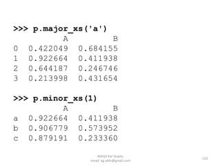
email: kg.abhi@gmail.com](https://image.slidesharecdn.com/akg-python-talk-numpy-pandas-190703192842/85/Python-for-Data-Science-and-Scientific-Computing-86-320.jpg)
![Series: Methods
>>> s.axes
[RangeIndex(start=0, stop=4, step=1)]
>>> s.values
array([10, 20, 30, 40], dtype=int64)
>>> s.size
4
>>> s.shape
(4,)
>>> s.ndim
1
>>> s.dtype
dtype('int64')
87
Abhijit Kar Gupta,
email: kg.abhi@gmail.com](https://image.slidesharecdn.com/akg-python-talk-numpy-pandas-190703192842/85/Python-for-Data-Science-and-Scientific-Computing-87-320.jpg)
![>>> s['e'] = 50
>>> s
a 10
b 20
c 30
d 40
e 50
dtype: int64
>>> data =['a', 'b', 'c', 'd']
>>> pd.Series(data)
0 a
1 b
2 c
3 d
dtype: object
88
Abhijit Kar Gupta,
email: kg.abhi@gmail.com](https://image.slidesharecdn.com/akg-python-talk-numpy-pandas-190703192842/85/Python-for-Data-Science-and-Scientific-Computing-88-320.jpg)
![# Data as scalar
>>> index = [‘a’, ‘b’, ‘c’, ‘d’]
>>> pd.Series(10, index, int)
a 10
b 10
c 10
d 10
dtype: int32
89
Abhijit Kar Gupta,
email: kg.abhi@gmail.com](https://image.slidesharecdn.com/akg-python-talk-numpy-pandas-190703192842/85/Python-for-Data-Science-and-Scientific-Computing-89-320.jpg)
![Series from Dictionary
>>> data = {'a':10, 'b':20, 'c':30, 'd':40}
>>> pd.Series(data)
a 10
b 20
c 30
d 40
dtype: int64
>>> index = ['a', 'b', 'c', 'd', 'e', 'f']
>>> pd.Series(data, index)
a 10.0
b 20.0
c 30.0
d 40.0
e NaN
f NaN
dtype: float64
90
Abhijit Kar Gupta,
email: kg.abhi@gmail.com](https://image.slidesharecdn.com/akg-python-talk-numpy-pandas-190703192842/85/Python-for-Data-Science-and-Scientific-Computing-90-320.jpg)

![>>> sum(s)
150L
>>> min(s)
10L
>>> max(s)
50L
>>> s[1:4]
b 20
c 30
d 40
dtype: int64
>>> s.sum()
100
>>> s.mean()
25.0
>>> s.std()
12.909944487358056
92
Abhijit Kar Gupta,
email: kg.abhi@gmail.com](https://image.slidesharecdn.com/akg-python-talk-numpy-pandas-190703192842/85/Python-for-Data-Science-and-Scientific-Computing-92-320.jpg)
![DataFrame
>>> x = [10,20,30,40]
>>> pd.DataFrame(x)
0
0 10
1 20
2 30
3 40
>>> x = [[10,20,30,40], [50,60,70,80]]
>>> pd.DataFrame(x)
0 1 2 3
0 10 20 30 40
1 50 60 70 80
93
Abhijit Kar Gupta,
email: kg.abhi@gmail.com](https://image.slidesharecdn.com/akg-python-talk-numpy-pandas-190703192842/85/Python-for-Data-Science-and-Scientific-Computing-93-320.jpg)
![>>> index = ['a','b']
>>> pd.DataFrame(x, index)
0 1 2 3
a 10 20 30 40
b 50 60 70 80
>>> d = pd.DataFrame(x,index,columns =
['A', 'B', 'C', 'D'])
A B C D
a 10 20 30 40
b 50 60 70 80
94
Abhijit Kar Gupta,
email: kg.abhi@gmail.com](https://image.slidesharecdn.com/akg-python-talk-numpy-pandas-190703192842/85/Python-for-Data-Science-and-Scientific-Computing-94-320.jpg)
![>>> d[‘A’]
a 10
b 50
>>> d[‘A’][‘a’]
10
95
Abhijit Kar Gupta,
email: kg.abhi@gmail.com](https://image.slidesharecdn.com/akg-python-talk-numpy-pandas-190703192842/85/Python-for-Data-Science-and-Scientific-Computing-95-320.jpg)
![Methods over DataFrame
• d.axes
• d.size
• d.ndim
• d.T
• d.empty
• d.values
• d.head(1)
• d.tail(1)
• d.sum()
• d.sum(1)
• d.mean()
• d.mean(1)[1]
• d.std()
• d.std(1)
• d.max()
• d.min()
• d.describe() # Full Statistics
96
Abhijit Kar Gupta,
email: kg.abhi@gmail.com](https://image.slidesharecdn.com/akg-python-talk-numpy-pandas-190703192842/85/Python-for-Data-Science-and-Scientific-Computing-96-320.jpg)
![DataFrame from the list of Dictionaries
>>> data = [{'x':2, 'y':10},{'x':4, 'y':20},{'x':6,
'y':30},{'x':8, 'y':40}]
>>> d = pd.DataFrame(data, index=[‘a’,’b’,’c’,’d’])
x y
a 2 10
b 4 20
c 6 30
d 8 40
>>> d['x']
a 2
b 4
c 6
d 8
Name: x, dtype: int64
>>> d['x'][‘b’]
4
97
Abhijit Kar Gupta,
email: kg.abhi@gmail.com](https://image.slidesharecdn.com/akg-python-talk-numpy-pandas-190703192842/85/Python-for-Data-Science-and-Scientific-Computing-97-320.jpg)
![DataFrame from Dictionary of Series
>>> index = ['a','b','c','d']
>>> s1 = pd.Series([10,20,30,40],index)
>>> s2 = pd.Series([100,200,300,400],index)
>>> d = {'A':s1, 'B':s2}
>>> pd.DataFrame(d)
A B
a 10 100
b 20 200
c 30 300
d 40 400
>>> D = pd.DataFrame(d)
>>> D['A']
a 10
b 20
c 30
d 40
Name: A, dtype: int64
98
Abhijit Kar Gupta,
email: kg.abhi@gmail.com](https://image.slidesharecdn.com/akg-python-talk-numpy-pandas-190703192842/85/Python-for-Data-Science-and-Scientific-Computing-98-320.jpg)
![Add column to DataFrame
>>> D['C']= pd.DataFrame({'C':pd.Series([1000,2000,3000,4000],index)})
>>> D
A B C
a 10 100 1000
b 20 200 2000
c 30 300 3000
d 40 400 4000
>>> D['C'] = pd.DataFrame(pd.Series([1000,2000,3000,4000],index))
>>> D
A B C
a 10 100 1000
b 20 200 2000
c 30 300 3000
d 40 400 4000
>>> D['C'] = pd.Series([1000,2000,3000,4000],index)
>>> D
A B C
a 10 100 1000
b 20 200 2000
c 30 300 3000
d 40 400 4000
99
Abhijit Kar Gupta,
email: kg.abhi@gmail.com](https://image.slidesharecdn.com/akg-python-talk-numpy-pandas-190703192842/85/Python-for-Data-Science-and-Scientific-Computing-99-320.jpg)
![Delete column and rows from DataFrame
>>> D
A B C
a 10 100 1000
b 20 200 2000
c 30 300 3000
d 40 400 4000
>>> del D['A']
>>> D
B C
a 100 1000
b 200 2000
c 300 3000
d 400 4000
100
Abhijit Kar Gupta,
email: kg.abhi@gmail.com](https://image.slidesharecdn.com/akg-python-talk-numpy-pandas-190703192842/85/Python-for-Data-Science-and-Scientific-Computing-100-320.jpg)
![Slicing
>>> D.loc['b']
A 20
B 200
C 2000
>>> D.iloc[1]
A 20
B 200
C 2000
Name: b, dtype: int64
>>> D[1:3]
A B C
b 20 200 2000
c 30 300 3000
>>> D[1:3]['A']
b 20
c 30
Name: A, dtype: int64
101
Abhijit Kar Gupta,
email: kg.abhi@gmail.com](https://image.slidesharecdn.com/akg-python-talk-numpy-pandas-190703192842/85/Python-for-Data-Science-and-Scientific-Computing-101-320.jpg)
![Append, Delete
>>> D1 = pd.DataFrame([[50,500,5000]], index =
['e'],columns=['A','B','C'])
>>> D1
A B C
e 50 500 5000
>>> D.append(D1) # Append another DataFrame
A B C
a 10 100 1000
b 20 200 2000
c 30 300 3000
d 40 400 4000
e 50 500 5000
>>> D.drop('a’) # Delete the indexed row.
A B C
b 20 200 2000
c 30 300 3000
d 40 400 4000
102
Abhijit Kar Gupta,
email: kg.abhi@gmail.com](https://image.slidesharecdn.com/akg-python-talk-numpy-pandas-190703192842/85/Python-for-Data-Science-and-Scientific-Computing-102-320.jpg)
![Re-indexing
>>> index = np.arange(1,6)
>>> d = pd.DataFrame(data, index, columns = ['x', 'y'])
>>> d
x y
1 0.1 0.2
2 0.3 0.4
3 0.5 0.6
4 0.7 0.8
5 0.9 1.0
>>> d.reindex(np.arange(2,7), ['x','y'])
x y
2 0.3 0.4
3 0.5 0.6
4 0.7 0.8
5 0.9 1.0
6 NaN NaN
103
Abhijit Kar Gupta,
email: kg.abhi@gmail.com](https://image.slidesharecdn.com/akg-python-talk-numpy-pandas-190703192842/85/Python-for-Data-Science-and-Scientific-Computing-103-320.jpg)
![Alignment of two DataFrames by
reindexing
>>> data = np.random.rand(10,3)
>>> d1 = pd.DataFrame(data, index = range(1,11), columns =
['x','y','z'])
>>> d1
x y z
1 0.342091 0.044060 0.773249
2 0.934012 0.038944 0.237909
3 0.670108 0.011794 0.831526
4 0.354686 0.381140 0.493882
5 0.690489 0.622695 0.409091
6 0.352255 0.205635 0.551726
7 0.371473 0.392713 0.853915
8 0.601222 0.353043 0.726287
9 0.933808 0.104148 0.718498
10 0.225576 0.812473 0.158370
104
Abhijit Kar Gupta,
email: kg.abhi@gmail.com](https://image.slidesharecdn.com/akg-python-talk-numpy-pandas-190703192842/85/Python-for-Data-Science-and-Scientific-Computing-104-320.jpg)
![>>> data = np.random.rand(8,3)
>>> d2 = pd.DataFrame(data, index = range(1,9),
columns = ['x','y','z'])
>>> d2
x y z
1 0.322780 0.376841 0.957168
2 0.892635 0.248012 0.705469
3 0.006545 0.050196 0.112410
4 0.886808 0.437421 0.658757
5 0.628429 0.961192 0.190440
6 0.374883 0.450280 0.983127
7 0.257246 0.776551 0.425495
8 0.939035 0.471483 0.810289
105
Abhijit Kar Gupta,
email: kg.abhi@gmail.com](https://image.slidesharecdn.com/akg-python-talk-numpy-pandas-190703192842/85/Python-for-Data-Science-and-Scientific-Computing-105-320.jpg)

![Panel
Panel is a 3D Container. DataFrame is a 2D container. Series is 1D.
>>> data = np.random.rand(2,3,4)
>>> np.random.rand(2,3,4)
array([[[0.05925325, 0.7165947 , 0.34978631, 0.68598632],
[0.51410651, 0.50950708, 0.99801304, 0.34533087],
[0.75854214, 0.50619351, 0.17673772, 0.4866736 ]],
[[0.49319432, 0.03183697, 0.61576345, 0.73591557],
[0.41456184, 0.20290885, 0.27732744, 0.63533898],
[0.64958528, 0.42573291, 0.13674149, 0.10115889]]])
>>> p = pd.Panel(data)
>>> p
<class 'pandas.core.panel.Panel'>
Dimensions: 2 (items) x 3 (major_axis) x 4 (minor_axis)
Items axis: 0 to 1
Major_axis axis: 0 to 2
Minor_axis axis: 0 to 3
107
Abhijit Kar Gupta,
email: kg.abhi@gmail.com](https://image.slidesharecdn.com/akg-python-talk-numpy-pandas-190703192842/85/Python-for-Data-Science-and-Scientific-Computing-107-320.jpg)
![>>> index = ['a','b','c']
>>> data = {'A': pd.DataFrame(np.random.rand(3,4),index),
'B':pd.DataFrame(np.random.rand(3,4),index)}
>>> p = pd.Panel(data)
>>> p
<class 'pandas.core.panel.Panel'>
Dimensions: 2 (items) x 3 (major_axis)
x 4 (minor_axis)
Items axis: A to B
Major_axis axis: a to c
Minor_axis axis: 0 to 3
109
Abhijit Kar Gupta,
email: kg.abhi@gmail.com](https://image.slidesharecdn.com/akg-python-talk-numpy-pandas-190703192842/85/Python-for-Data-Science-and-Scientific-Computing-109-320.jpg)
![Methods on Panel
>>> p.values
array([[[0.42204928, 0.92266448, 0.64418741, 0.21399842],
[0.42902311, 0.90677907, 0.67544671, 0.60858596],
[0.35946858, 0.87919109, 0.16145494, 0.46737675]],
[[0.68415499, 0.411938 , 0.24674607, 0.43165447],
[0.15053089, 0.57395153, 0.65095238, 0.7393423 ],
>>> p.axes
[Index([u'A', u'B'], dtype='object'), Index([u'a', u'b',
u'c'], dtype='object'), RangeIndex(start=0, stop=4,
step=1)]
>>> p.size
24
>>> p.ndim
3
>>> p.shape
(2, 3, 4)
111
Abhijit Kar Gupta,
email: kg.abhi@gmail.com](https://image.slidesharecdn.com/akg-python-talk-numpy-pandas-190703192842/85/Python-for-Data-Science-and-Scientific-Computing-111-320.jpg)


Python for Data Science and Scientific Computing
- 1. Python for Scientific Computing and Data Science 1 Abhijit Kar Gupta, email: kg.abhi@gmail.com
- 2. Arrays and Data Structures • Numpy • Pandas 2 Abhijit Kar Gupta, email: kg.abhi@gmail.com
- 3. ND Arrays by Numpy >>> import numpy as np >>> x = np.array([10, 20, 30]) >>> 10 in x True >>> 11 in x False 3 Abhijit Kar Gupta, email: kg.abhi@gmail.com
- 4. Attributes: Type, Size, Dimension >>> x = np.array([10, 20, 30]) >>> type(x) <type 'numpy.ndarray'> >>> x.size 3 >>> x.dtype dtype('int32') >>> x.ndim 1 4 Abhijit Kar Gupta, email: kg.abhi@gmail.com
- 5. >>> y = np.array([[1,2,3],[4,5,6]]) >>> y array([[1, 2, 3], [4, 5, 6]]) >>> y.ndim 2 >>> y.size 6 5 Abhijit Kar Gupta, email: kg.abhi@gmail.com
- 6. >>> M = np.array([[[1,2],[3,4]], [[5,6],[7,8]]]) >>> M array([[[1, 2], [3, 4]], [[5, 6], [7, 8]]]) >>> M.ndim 3 6 Abhijit Kar Gupta, email: kg.abhi@gmail.com
- 7. Data Type • int8 (1 byte = 8-bit: Integer -128 to 127), int16 (-32768 to 32767), int32, int64 • uint8 (unsigned integer: 0 to 255), uint16, uint32, uint64 • float16 (half precision float: sign bit, 5 bits exponent, 10 bits mantissa), float32 (single precision: sign bit, 8 bits exponent, 10 bits mantissa), float64 (double precision: sign bit, 11 bit exponent, 52 bits mantissa) • complex64 (complex number, represented by two 32-bit floats: real and imaginary components), complex128 (complex number, represented by two 64-bit floats: real and imaginary components) Acronyms: i1 = int8, i2 = int16, i3 = int32, i4 = int64 f2 = float16, f4 = float32, f8 = float64 7 Abhijit Kar Gupta, email: kg.abhi@gmail.com
- 8. Default Data type >>> x = np.array([10, 23, 36, 467]) >>> x.dtype dtype('int32') >>> y = np.array([10.5, 23, 36, 467]) >>> y.dtype dtype('float64') >>> a = np.array(['ab','bc', 'ca', 100]) >>> a array(['ab', 'bc', 'ca', '100'], dtype='|S3') *S3 = String of length 3. 8 Abhijit Kar Gupta, email: kg.abhi@gmail.com
- 9. Given Data type >>> x = np.array([10,20,30], dtype = 'f') >>> x array([10., 20., 30.], dtype = float32) >>> x = np.array([10.5,23,36,467], dtype = 'f4') >>> x array([ 10.5, 23. , 36. , 467. ], dtype = float32) >>> x = np.array([10.5,23,36,467], dtype = 'complex') >>> x array([ 10.5+0.j, 23. +0.j, 36. +0.j, 467. +0.j]) >>> x.dtype dtype('complex128') >>> x = np.array([10.5,23,36,467], dtype = 'complex64') >>> x.dtype dtype('complex64') 9 Abhijit Kar Gupta, email: kg.abhi@gmail.com
- 10. >>> A = np.array(['ab', 'bc', 'ca', 100], dtype = 'S10') >>> A array(['ab', 'bc', 'ca', '100'], dtype='|S10') >>> A = np.array(['ab','bc', 'ca', 'abracadabra', 100], dtype = 'S6') >>> A array(['ab', 'bc', 'ca', 'abraca', '100'], dtype= '|S6') >>> A.itemsize # Size of each item 6 10 Abhijit Kar Gupta, email: kg.abhi@gmail.com
- 11. Methods for creation of arrays np.arange(start, stop, step) >>> np.arange(3) array([0, 1, 2]) >>> np.arange(3.0) array([0., 1., 2.]) >>> np.arange(3, 15, 2, dtype ='float') array([ 3., 5., 7., 9., 11., 13.]) >>> np.arange(0.5, 1.0, 0.1) array([0.5, 0.6, 0.7, 0.8, 0.9]) 11 Abhijit Kar Gupta, email: kg.abhi@gmail.com
- 12. np.linspace(start, end, num) >>> np.linspace(10, 20, 5) array([10. , 12.5, 15. , 17.5, 20. ]) >>> np.linspace(10, 20, 5, endpoint = True) array([10. , 12.5, 15. , 17.5, 20. ]) >>> np.linspace(10, 20, 5, endpoint = False) array([10., 12., 14., 16., 18.]) >>> np.linspace(10, 20, 5, retstep = True) (array([10. , 12.5, 15. , 17.5, 20. ]), 2.5) # returns step value 12 Abhijit Kar Gupta, email: kg.abhi@gmail.com
- 13. # Evenly spaced in logscale >>> np.logspace(0, 1, 10) array([ 1., 1.29154967, 1.66810054, 2.15443469, 2.7825594,3.59381366, 4.64158883, 5.9948425, 7.74263683, 10.]) # 10 vales, default base = 10 >>> x = np.logspace(0, 1, 10) >>> np.log10(x) array([0., 0.11111111, 0.22222222, 0.33333333, 0.44444444, 0.55555556, 0.66666667, 0.77777778, 0.88888889, 1.]) >>> np.logspace(0, 1, 10, base = 2) array([1., 1.08005974, 1.16652904, 1.25992105, 1.36079,1.46973449, 1.58740105, 1.71448797, 1.85174942, 2.]) 13 Abhijit Kar Gupta, email: kg.abhi@gmail.com
- 14. Shape/Reshape >>> a = np.arange(0,60,5) >>> a array([ 0, 5, 10, 15, 20, 25, 30, 35, 40, 45, 50, 55]) >>> np.shape(a) (12,) >>> a.shape (12,) >>> np.reshape(a, (3,4)) array([[ 0, 5, 10, 15], [20, 25, 30, 35], [40, 45, 50, 55]]) >>> b = a.reshape(3,4) >>> np.shape(b) (3, 4) >>> b.shape (3, 4) 14 Abhijit Kar Gupta, email: kg.abhi@gmail.com
- 15. Unique elements >>> y = np.array([1,2,1,0.5,10,2,10]) >>> np.unique(y) array([ 0.5, 1. , 2. , 10. ]) >>> L = np.random.randint(0, 2, (4,5)) >>> L array([[0, 1, 0, 0, 0], [0, 1, 1, 1, 0], [1, 0, 1, 0, 0], [0, 1, 0, 1, 1]]) >>> np.unique(L) array([0, 1]) >>> A = np.array(['a', 'b', 'c', 'a', 'b', 'a']) >>> np.unique(A) array(['a', 'b', 'c'], dtype='|S1') 15 Abhijit Kar Gupta, email: kg.abhi@gmail.com
- 16. Iterator >>> import numpy as np >>> x = np.array([10, 20, 30, 40]) >>> for i in x: print i 10 20 30 40 >>> A = np.arange(0,60,5).reshape(3, 4) >>> for i in A: print i [ 0 5 10 15] [20 25 30 35] [40 45 50 55] 16 Abhijit Kar Gupta, email: kg.abhi@gmail.com
- 17. >>> for i in np.nditer(A, order = 'F'): print i 0 20 40 5 25 45 10 30 50 15 35 55 17 Abhijit Kar Gupta, email: kg.abhi@gmail.com
- 18. >>> for i in np.nditer(a, order = 'C'): print i 0 5 10 15 20 25 30 35 40 45 50 55 18 Abhijit Kar Gupta, email: kg.abhi@gmail.com
- 19. Inserting Elements >>> a = np.array([0, -1, 2, 5, 10]) >>> a.put(3, 99) >>> a array([ 0, -1, 2, 99, 10]) >>> np.insert(a, 3, 99) array([ 0, -1, 2, 99, 5, 10]) 19 Abhijit Kar Gupta, email: kg.abhi@gmail.com
- 20. >>> A = np.array([[1,2], [3,4]]) >>> A array([[1, 2], [3, 4]]) >>> np.insert(A, 1, [10, 12], axis = 0) array([[ 1, 2], [10, 12], [ 3, 4]]) >>> np.insert(A, 1, [10, 12], axis = 1) array([[ 1, 10, 2], [ 3, 12, 4]]) 20 Abhijit Kar Gupta, email: kg.abhi@gmail.com
- 21. >>> np.insert(A, 1, [10, 12]) array([ 1, 10, 12, 2, 3, 4]) # Flattened when without axis ref >>> np.insert(A, 1, [10]) array([ 1, 10, 2, 3, 4]) >>> np.insert(A, 1, [10], axis = 0) array([[ 1, 2], [10, 10], [ 3, 4]]) >>> np.insert(A, 1, [10], axis = 1) array([[ 1, 10, 2], [ 3, 10, 4]]) >>> np.insert(A, 1, [10,12], axis = 0) array([[ 1, 2], [10, 12], [ 3, 4]]) 21 Abhijit Kar Gupta, email: kg.abhi@gmail.com
- 22. Deleting >>> x = np.arange(1, 13).reshape(3,4) >>> x array([[ 1, 2, 3, 4], [ 5, 6, 7, 8], [ 9, 10, 11, 12]]) >>> np.delete(x, 2, axis = 0) array([[1, 2, 3, 4], [5, 6, 7, 8]]) >>> np.delete(x, 2, axis = 1) array([[ 1, 2, 4], [ 5, 6, 8], [ 9, 10, 12]]) 22 Abhijit Kar Gupta, email: kg.abhi@gmail.com
- 23. Split >>> np.split(x, 3) [array([[1, 2, 3, 4]]), array([[5, 6, 7, 8]]), array([[ 9, 10, 11, 12]])] >>> np.vsplit(x, 3) # same as above (row wise split) >>> np.hsplit(x, 4) [array([[1], [5], [9]]), array([[ 2], [ 6], [10]]), array([[ 3], [ 7], [11]]), array([[ 4], [ 8], [12]])] 23 Abhijit Kar Gupta, email: kg.abhi@gmail.com
- 24. Append >>> x = np.array([1, 2, 3, 4]) >>> np.append(x, 7) array([1, 2, 3, 4, 7]) >>> x = np.array([10, 20, 30]) >>> y = np.array([100, 200, 300]) >>> np.append(x, y) array([ 10, 20, 30, 100, 200, 300]) 24 Abhijit Kar Gupta, email: kg.abhi@gmail.com
- 25. >>> A = np.array([[1,2], [3,4]]) >>> A array([[1, 2], [3, 4]]) >>> np.append(A, 99) array([ 1, 2, 3, 4, 99]) #flattens and appends >>> np.append(A, [[9,10]], axis = 0) array([[ 1, 2], [ 3, 4], [ 9, 10]]) 25 Abhijit Kar Gupta, email: kg.abhi@gmail.com
- 26. Complex arrays >>> x = np.array([2+3j, 5+2j, 3-1j]) >>> x.real array([2., 5., 3.]) >>> x.imag array([ 3., 2., -1.]) >>> x.conj() array([2.-3.j, 5.-2.j, 3.+1.j]) 26 Abhijit Kar Gupta, email: kg.abhi@gmail.com
- 27. Statistics >>> x = np.arange(10, 100, 10) >>> x array([10, 20, 30, 40, 50, 60, 70, 80, 90]) >>> np.sum(x) 450 >>> np.cumsum(x) array([ 10, 30, 60, 100, 150, 210, 280, 360, 450]) >>> x = np.arange(10, 100, 10).reshape(3,3) >>> x array([[10, 20, 30], [40, 50, 60], [70, 80, 90]]) >>> np.sum(x) 450 >>> np.sum(x, 0) # 0 axis array([120, 150, 180]) >>> np.sum(x, 1) # 1 axis 27 Abhijit Kar Gupta, email: kg.abhi@gmail.com
- 28. >>> np.trace(x) 150 >>> np.trace(x, 1) 80 >>> np.trace(x, -1) 120 >>> np.mean(x) 50.0 >>> np.mean(x,1) array([20., 50., 80.]) >>> np.mean(x,0) array([40., 50., 60.]) >>> np.median(x) 50.0 >>> np.median(x,0) array([40., 50., 60.]) >>> np.median(x,1) array([20., 50., 80.]) 28 Abhijit Kar Gupta, email: kg.abhi@gmail.com
- 29. >>> x = np.array([0, -1, 2, 5, 10, 3, -2, 4]) >>> np.ptp(x) # peak to peak 12 >>> np.var(x) # variance 12.984375 >>> np.std(x) # standard dev 3.6033838263498934 29 Abhijit Kar Gupta, email: kg.abhi@gmail.com
- 30. >>> x = np.array([0, -1, 2, 5, 10, 3, -2, 4]).reshape(2,4) >>> x array([[ 0, -1, 2, 5], [10, 3, -2, 4]]) >>> np.ptp(x, 0) array([10, 4, 4, 1]) >>> np.ptp(x, 1) array([ 6, 12]) 30 Abhijit Kar Gupta, email: kg.abhi@gmail.com
- 31. Sorting >>> L = np.random.randint(-10, 10, (4,5)) >>> L array([[-6, -4, -7, 5, 6], [ 0, -9, -8, -4, -1], [ 0, 8, -5, 0, 2], [-8, -5, -2, -2, -8]]) >>> np.sort(L) array([[-7, -6, -4, 5, 6], [-9, -8, -4, -1, 0], [-5, 0, 0, 2, 8], [-8, -8, -5, -2, -2]]) >>> np.sort(L, 0) array([[-8, -9, -8, -4, -8], [-6, -5, -7, -2, -1], [ 0, -4, -5, 0, 2], [ 0, 8, -2, 5, 6]]) >>> np.sort(L, 1) array([[-7, -6, -4, 5, 6], [-9, -8, -4, -1, 0], [-5, 0, 0, 2, 8], [-8, -8, -5, -2, -2]]) 31 Abhijit Kar Gupta, email: kg.abhi@gmail.com
- 32. Concatenation >>> x = np.array([10,20,30]) >>> y = np.array([40,50,60]) >>> np.concatenate((x,y)) array([10, 20, 30, 40, 50, 60]) 32 Abhijit Kar Gupta, email: kg.abhi@gmail.com
- 33. >>> x = np.array([[1,2,3],[4,5,6]]) >>> y = np.array([[7,8,9],[10,11,12]]) >>> np.concatenate((x,y)) array([[1, 2, 3], [4, 5, 6], [7, 8, 9], [10, 11, 12]]) >>> np.concatenate((x,y), axis = 1) array([[1, 2, 3, 7, 8, 9], [4, 5, 6, 10, 11, 12]]) 33 Abhijit Kar Gupta, email: kg.abhi@gmail.com
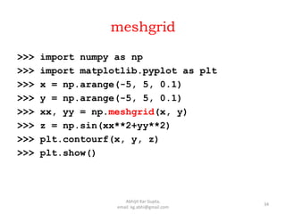
- 34. meshgrid >>> import numpy as np >>> import matplotlib.pyplot as plt >>> x = np.arange(-5, 5, 0.1) >>> y = np.arange(-5, 5, 0.1) >>> xx, yy = np.meshgrid(x, y) >>> z = np.sin(xx**2+yy**2) >>> plt.contourf(x, y, z) >>> plt.show() 34 Abhijit Kar Gupta, email: kg.abhi@gmail.com
- 35. mgrid >>> xx, yy = np.mgrid[-5:5:0.1, -5:5:0.1] >>> x = xx[:,0] >>> y = yy[0,:] >>> xx array([[-5. , -5. , -5. , ..., -5. , -5. , -5. ], [-4.9, -4.9, -4.9, ..., -4.9, -4.9, -4.9], [-4.8, -4.8, -4.8, ..., -4.8, -4.8, -4.8], ..., [ 4.7, 4.7, 4.7, ..., 4.7, 4.7, 4.7], [ 4.8, 4.8, 4.8, ..., 4.8, 4.8, 4.8], [ 4.9, 4.9, 4.9, ..., 4.9, 4.9, 4.9]]) >>> yy array([[-5. , -4.9, -4.8, ..., 4.7, 4.8, 4.9], [-5. , -4.9, -4.8, ..., 4.7, 4.8, 4.9], [-5. , -4.9, -4.8, ..., 4.7, 4.8, 4.9], ..., [-5. , -4.9, -4.8, ..., 4.7, 4.8, 4.9], [-5. , -4.9, -4.8, ..., 4.7, 4.8, 4.9], [-5. , -4.9, -4.8, ..., 4.7, 4.8, 4.9]]) 35 Abhijit Kar Gupta, email: kg.abhi@gmail.com
- 36. 36 Abhijit Kar Gupta, email: kg.abhi@gmail.com
- 37. Special arrays >>> np.eye(3) array([[1., 0., 0.], [0., 1., 0.], [0., 0., 1.]]) >>> np.zeros(3) array([0., 0., 0.]) >>> np.zeros((3,3)) array([[0., 0., 0.], [0., 0., 0.], [0., 0., 0.]]) >>> np.full((3,3),5) array([[5, 5, 5], [5, 5, 5], [5, 5, 5]]) 37 Abhijit Kar Gupta, email: kg.abhi@gmail.com
- 38. >>> a = np.array([[1,2],[3,4]]) >>> a array([[1, 2], [3, 4]]) >>> np.zeros_like(a) array([[0, 0], [0, 0]]) >>> np.diag((1,2,3)) array([[1, 0, 0], [0, 2, 0], [0, 0, 3]]) >>> np.diag((1,2,3), k = 1) array([[0, 1, 0, 0], [0, 0, 2, 0], [0, 0, 0, 3], [0, 0, 0, 0]]) 38 Abhijit Kar Gupta, email: kg.abhi@gmail.com
- 39. Indexing, Slicing >>> x = np.arange(2, 15, 3) >>> x array([2, 5, 8, 11, 14]) >>> x[0] 2 >>> x[2] 8 >>> x[-1] 14 >>> x[1:5:2] array([5, 11]) Also, one can write: s = slice(1,5,2) and then x[s] 39 Abhijit Kar Gupta, email: kg.abhi@gmail.com
- 40. >>> x[3:] array([11, 14]) >>> x[:4] array([ 2, 5, 8, 11]) >>> x[::2] array([ 2, 8, 14]) >>> x[2::] array([ 8, 11, 14]) >>> x[::-1] array([14, 11, 8, 5, 2]) >>> x[::-3] array([14, 5]) 40 Abhijit Kar Gupta, email: kg.abhi@gmail.com
- 41. >>> x = np.arange(12).reshape(4,3) >>> x array([[ 0, 1, 2], [ 3, 4, 5], [ 6, 7, 8], [ 9, 10, 11]]) >>> x[2:] array([[ 6, 7, 8], [ 9, 10, 11]]) >>> x[:3] array([[0, 1, 2], [3, 4, 5], [6, 7, 8]]) >>> x[::2] array([[0, 1, 2], [6, 7, 8]]) 41 Abhijit Kar Gupta, email: kg.abhi@gmail.com
- 42. >>> x[:] array([[ 0, 1, 2, 3], [ 4, 5, 6, 7], [ 8, 9, 10, 11]]) >>> x[:,0] array([0, 4, 8]) >>> x[:,1:3] array([[ 1, 2], [ 5, 6], [ 9, 10]]) >>> x[1:3, 1:3] array([[ 5, 6], [ 9, 10]]) 42 Abhijit Kar Gupta, email: kg.abhi@gmail.com
- 43. >>> x[x > 3] array([ 4, 5, 6, 7, 8, 9, 10, 11]) # returns the elements in 1D array >>> x.flatten() array([ 0, 1, 2, 3, 4, 5, 6, 7, 8, 9, 10, 11]) >>> x.flatten(0) array([ 0, 1, 2, 3, 4, 5, 6, 7, 8, 9, 10, 11]) >>> x.flatten(1) array([ 0, 3, 6, 9, 1, 4, 7, 10, 2, 5, 8, 11]) 43 Abhijit Kar Gupta, email: kg.abhi@gmail.com
- 44. Arithmetic Operations >>> x = np.array([1, 2, 3, 4]) >>> y = np.array([5, 6, 7, 8]) >>> x*y array([ 5, 12, 21, 32]) >>> x+y array([ 6, 8, 10, 12]) >>> x-y array([-4, -4, -4, -4]) >>> x/y array([0, 0, 0, 0]) >>> x**y array([ 1, 64, 2187, 65536]) 44 Abhijit Kar Gupta, email: kg.abhi@gmail.com
- 45. >>> x = np.arange(1,7).reshape(2,3) >>> x array([[1, 2, 3], [4, 5, 6]]) >>> y = np.array([10, 11, 12]) >>> x + y array([[11, 13, 15], [14, 16, 18]]) >>> x + 2 array([[3, 4, 5], [6, 7, 8]]) >>> x + [2, 3, 4] array([[ 3, 5, 7], [ 6, 8, 10]]) * Broadcasting! 45 Abhijit Kar Gupta, email: kg.abhi@gmail.com
- 46. Array manipulation >>> x array([[1, 2, 3], [4, 5, 6]]) >>> x.T array([[1, 4], [2, 5], [3, 6]]) >>> x.transpose() array([[1, 4], [2, 5], [3, 6]]) 46 Abhijit Kar Gupta, email: kg.abhi@gmail.com
- 47. Stacking >>> x array([[1, 2], [3, 4]]) >>> y array([[5, 6], [7, 8]]) >>> np.stack((x,y)) # default axis = 0 array([[[1, 2], [3, 4]], [[5, 6], [7, 8]]]) >>> np.stack((x,y),axis = 1) array([[[1, 2], [5, 6]], [[3, 4], [7, 8]]]) 47 Abhijit Kar Gupta, email: kg.abhi@gmail.com
- 48. >>> np.vstack((x, y)) # stacks vertically array([[1, 2], [3, 4], [5, 6], [7, 8]]) >>> np.hstack((x, y)) # stacks horizontally array([[1, 2, 5, 6], [3, 4, 7, 8]]) 48 Abhijit Kar Gupta, email: kg.abhi@gmail.com
- 49. Numpy Functions Functions over arrays >>> import numpy as np >>> x = np.arange(0, 1, 0.1) >>> x array([0. , 0.1, 0.2, 0.3, 0.4, 0.5, 0.6, 0.7, 0.8, 0.9]) >>> np.sin(x) array([0., 0.09983342, 0.19866933, 0.29552021, 0.38941834, 0.47942554, 0.56464247, 0.64421769, 0.71735609, 0.78332691]) >>> f = lambda x: x**2 >>> f(x) array([0., 0.01, 0.04, 0.09, 0.16, 0.25, 0.36, 0.49, 0.64, 0.81]) 49 Abhijit Kar Gupta, email: kg.abhi@gmail.com
- 50. >>> x = range(1, 5) >>> x [1, 2, 3, 4] >>> np.sqrt(x) array([1., 1.41421356, 1.73205081, 2. ]) >>> f = lambda x: x**2 >>> f(x) Traceback (most recent call last): File "<pyshell#85>", line 1, in <module> f(x) File "<pyshell#84>", line 1, in <lambda> f = lambda x: x**2 TypeError: unsupported operand type(s) for ** or pow(): 'list' and 'int' 50 Abhijit Kar Gupta, email: kg.abhi@gmail.com
- 51. Vectorize >>> f1 = np.vectorize(f) >>> type(f1) <class 'numpy.vectorize'> >>> f1(x) array([ 1, 4, 9, 16]) 51 Abhijit Kar Gupta, email: kg.abhi@gmail.com
- 52. Arrays as Vectors # Inner Product >>> u = np.array([1,2,3]) >>> v = np.array([-1,0,1]) >>> np.inner(u,v) 2 >>> np.inner(u, 2) array([2, 4, 6]) >>> np.inner(np.eye(3),5)) array([[5., 0., 0.], [0., 5., 0.], [0., 0., 5.]]) 52 Abhijit Kar Gupta, email: kg.abhi@gmail.com
- 53. # Multidimensional inner product >>> A = np.array([[1,2,3],[4,5,6]]) >>> B = np.array([[1,0,1],[0,1,0]]) >>> np.inner(A,B) array([[ 4, 2], [10, 5]]) 53 Abhijit Kar Gupta, email: kg.abhi@gmail.com
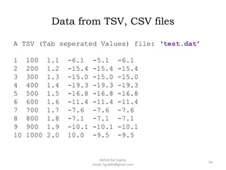
- 54. Data from TSV, CSV files A TSV (Tab seperated Values) file: ‘test.dat’ 1 100 1.1 -6.1 -5.1 -6.1 2 200 1.2 -15.4 -15.4 -15.4 3 300 1.3 -15.0 -15.0 -15.0 4 400 1.4 -19.3 -19.3 -19.3 5 500 1.5 -16.8 -16.8 -16.8 6 600 1.6 -11.4 -11.4 -11.4 7 700 1.7 -7.6 -7.6 -7.6 8 800 1.8 -7.1 -7.1 -7.1 9 900 1.9 -10.1 -10.1 -10.1 10 1000 2.0 10.0 -9.5 -9.5 54 Abhijit Kar Gupta, email: kg.abhi@gmail.com
- 55. >>> data = np.genfromtxt('test.dat') >>> data array([[ 1. , 100. , 1.1, -6.1, -5.1, -6.1], [ 2. , 200. , 1.2, -15.4, -15.4, -15.4], [ 3. , 300. , 1.3, -15. , -15. , -15. ], [ 4. , 400. , 1.4, -19.3, -19.3, -19.3], [ 5. , 500. , 1.5, -16.8, -16.8, -16.8], [ 6. , 600. , 1.6, -11.4, -11.4, -11.4], [ 7. , 700. , 1.7, -7.6, -7.6, -7.6], [ 8. , 800. , 1.8, -7.1, -7.1, -7.1], [ 9. , 900. , 1.9, -10.1, -10.1, -10.1], [ 10. , 1000. , 2. , 10. , -9.5, -9.5]]) >>> data = np.loadtxt('test.dat') >>> R = np.random.randint(1, 10, (3,4)) >>> R array([[7, 5, 1, 2], [8, 4, 9, 4], [9, 4, 6, 7]]) >>> np.savetxt('random.dat', R) 55 Abhijit Kar Gupta, email: kg.abhi@gmail.com
- 56. # Vector Cross Product >>> x = np.array([1, 2, 3]) >>> y = np.array([-1,3, 0]) >>> np.cross(x, y) array([-9, -3, 5]) Volume of a Parallelepiped: Three sides are given by three vectors: 𝑨 = 𝟐𝒊 − 𝟑𝒋, 𝑩 = 𝒊 + 𝒋 − 𝒌, 𝑪 = 𝟑𝒊 − 𝒌 Volume = 𝑨. 𝑩 × 𝑪 = 𝟒 >>> a = np.array([2, -3, 0]) >>> b = np.array([1, 1, -1]) >>> c = np.array([3, 0, -1]) >>> np.vdot(a, np.cross(b, c)) 4 56 Abhijit Kar Gupta, email: kg.abhi@gmail.com
- 57. Matrix Like Operations >>> A = np.array([[1,2,3],[4,5,6]]) >>> B = np.array([[1,2],[3,4],[5,6]]) >>> np.dot(A,B) array([[22, 28], [49, 64]]) >>> A.dot(B) array([[22, 28], [49, 64]]) >>> B.dot(A) array([[ 9, 12, 15], [19, 26, 33], [29, 40, 51]]) AB ≠ BA 57 Abhijit Kar Gupta, email: kg.abhi@gmail.com
- 58. Matrix >>> X = np.matrix(A) >>> Y = np.matrix(B) >>> X*Y matrix([[22, 28], [49, 64]]) >>> Y*X matrix([[ 9, 12, 15], [19, 26, 33], [29, 40, 51]]) 58 Abhijit Kar Gupta, email: kg.abhi@gmail.com
- 59. Complex Matrix >>> C = np.matrix([[1+2j, 1j], [2-3j, 4j]]) >>> C matrix([[1.+2.j, 0.+1.j], [2.-3.j, 0.+4.j]]) >>> C.T matrix([[1.+2.j, 2.-3.j], [0.+1.j, 0.+4.j]]) >>> C.conjugate() matrix([[1.-2.j, 0.-1.j], [2.+3.j, 0.-4.j]]) >>> np.angle(C) matrix([[ 1.10714872, 1.57079633], [-0.98279372, 1.57079633]]) >>> C.H #Adjoint Matrix matrix([[1.-2.j, 2.+3.j], [0.-1.j, 0.-4.j]]) 59 Abhijit Kar Gupta, email: kg.abhi@gmail.com
- 60. Eigen values, Eigen vectors >>> import numpy as np >>> import numpy.linalg as lin >>> A = np.array([[1,2],[3,4]]) >>> lin.eig(A) (array([-0.37228132, 5.37228132]), array([[-0.82456484, -0.41597356],[ 0.56576746, -0.90937671]])) >>> eigen_val, eigen_vec = lin.eig(A) 60 Abhijit Kar Gupta, email: kg.abhi@gmail.com
- 61. >>> eigen_val array([-0.37228132, 5.37228132]) >>> eigen_vec array([[-0.82456484, -0.41597356], [ 0.56576746, -0.90937671]]) >>> eigen_vec[:,0] array([-0.82456484, 0.56576746]) >>> eigen_vec[:,1] array([-0.41597356, -0.90937671]) 61 Abhijit Kar Gupta, email: kg.abhi@gmail.com
- 62. Linear Algebra 𝑥1 + 2𝑥2 − 𝑥3 = 1 2𝑥1 + 𝑥2 +4𝑥3 = 2 3𝑥1 + 3𝑥2 + 4𝑥3 = 1 A = 1 2 −1 2 1 4 3 3 4 , x = 𝑥1 𝑥2 𝑥3 , and b = 1 2 1 >>> import numpy as np >>> a = np.array([[1,2,-1],[2,1,4],[3,3,4]]) >>> b = np.array([1,2,1]) >>> print np.linalg.solve(a,b) [ 7. -4. -2.] 62 Abhijit Kar Gupta, email: kg.abhi@gmail.com
- 63. Matrix Inverse >>> import numpy as np >>> A = np.array([[1,1,1], [1,2,3], [1,4,9]]) >>> Ainv = np.linalg.inv(A) >>> Ainv array([[ 3. , -2.5, 0.5], [-3. , 4. , -1. ], [ 1. , -1.5, 0.5]]) 63 Abhijit Kar Gupta, email: kg.abhi@gmail.com
- 64. Polynomial by Numpy >>> from numpy import poly1d >>> p = np.poly1d([1,2,3]) >>> print p 1 𝑥2 + 2 𝑥 + 3 >>> p(2) 11 >>> p(-1) 2 >>> p.c # Coefficients array([1, 2, 3]) >>> p.order # Order of the polynomial 2 64 Abhijit Kar Gupta, email: kg.abhi@gmail.com
- 65. Methods on Polynomials >>> from numpy import poly1d as poly >>> p1 = poly([1,5,6]) >>> p2 = poly([1,2]) >>> p1 + p2 poly1d([1, 6, 8]) >>> p1*p2 poly1d([ 1, 7, 16, 12]) >>> p1/p2 (poly1d([1., 3.]), poly1d([0.])) >>> p2**2 poly1d([1, 4, 4]) >>> from numpy import sin >>> sin(p2) array([0.84147098, 0.90929743]) 65 Abhijit Kar Gupta, email: kg.abhi@gmail.com
- 66. >>> p = np.poly1d([1, -5, 6]) >>> p.r array([3., 2.]) # Real roots: 3, 2 >>> p.deriv(1) # First derivative poly1d([2, 2]) >>> p.deriv(2) # Second derivative poly1d([2]) >>> p.integ(1) poly1d([0.33333333, 1. , 3. , 0. ]) >>> p.integ(2) poly1d([0.08333333, 0.33333333,1.5,0.,0. ]) 66 Abhijit Kar Gupta, email: kg.abhi@gmail.com
- 67. Plotting by Matplotlib >>> import matplotlib.pyplot as plt >>> x = [1, 2, 3, 4, 5] >>> y = [1, 4, 9, 16, 25] >>> plt.plot(x, y) [<matplotlib.lines.Line2D object at 0x000000000BE00B70>] >>> plt.show() 67 Abhijit Kar Gupta, email: kg.abhi@gmail.com
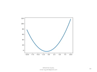
- 68. To plot the polynomial and see… 68 >>> import numpy as np >>> import matplotlib.pyplot as plt >>> x = np.linspace(-10,10,100) >>> p = np.poly1d([1, 2, -3]) >>> y = p(x) >>> plt.plot(x, y, lw = 3) [<matplotlib.lines.Line2D object at 0x000000000C27A860>] >>> plt.show() Abhijit Kar Gupta, email: kg.abhi@gmail.com
- 69. 69 Abhijit Kar Gupta, email: kg.abhi@gmail.com
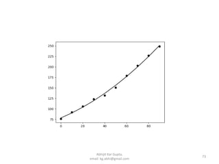
- 70. Curve fitting by Polynomial 𝑥 0 10 20 30 40 50 60 70 80 90 𝑦 76 92 106 123 132 151 179 203 227 249 70 To fit the following data by a polynomial… Abhijit Kar Gupta, email: kg.abhi@gmail.com
- 71. Step 1: >>> import numpy as np >>> x = np.array([0,10,20,30,40,50,60,70,80,90]) >>> y = np.array([76,92,106,123,132,151,179,203,227,249]) Step 2: >>> import numpy.polynomial.polynomial as poly >>> coeffs = poly.polyfit(x, y, 2) >>> coeffs array([7.81909091e+01, 1.10204545e+00, 9.12878788e-03]) Step 3: >>> yfit = poly.polyval(x,coeffs) >>> yfit array([ 78.19090909, 90.12424242, 103.88333333, 119.46818182,136.87878788, 156.11515152, 177.17727273, 200.06515152,224.77878788, 251.31818182]) Step 4: >>> import matplotlib.pyplot as plt >>> plt.plot(x, y, x, yfit ) >>> plt.show() 71 Abhijit Kar Gupta, email: kg.abhi@gmail.com
- 72. Python Script for Polynomial fitting # Polynomial fitting by Numpy (with plot) import numpy as np import numpy.polynomial.polynomial as poly import matplotlib.pyplot as plt x = np.array([0,10,20,30,40,50,60,70,80,90]) y = np.array([76,92,106,123,132,151,179,203,227,249]) coeffs = poly.polyfit(x, y, 2) yfit = poly.polyval(x, coeffs) plt.plot(x, y, 'ko', x, yfit, 'k-') plt.title('Fitting by polyfit', size = '20') plt.show() 72 Abhijit Kar Gupta, email: kg.abhi@gmail.com
- 73. 73 Abhijit Kar Gupta, email: kg.abhi@gmail.com
- 74. Fitting with user defined function # Input Data >>> import numpy as np >>> x = np.array([0,10,20,30,40,50,60,70,80,90]) >>> y = np.array([76,92,106,123,132,151,179,203,227,249]) # Define fitting function >>> def f(x,a,b,c): return a*x**2 + b*x + c # Optimize the parameters >>> from scipy.optimize import curve_fit >>> par, var = curve_fit(f, x, y) >>> a, b, c = par # To plot and show >>> import matplotlib.pyplot as plt >>> plt.plot(x, y, x, f(x,a,b,c)) >>> plt.show() 74 Abhijit Kar Gupta, email: kg.abhi@gmail.com
- 75. Example Script: Fitting with user defined function import numpy as np import matplotlib.pyplot as plt from scipy.optimize import curve_fit x = np.array([-8, -6, -4, -2, -1, 0, 1, 2, 4, 6, 8]) y = np.array([99, 610, 1271, 1804, 1900, 1823, 1510, 1346, 635, 125, 24]) def f(x, a, b, c): return a*np.exp(-b*(x-c)**2) par, var = curve_fit(f,x,y) a, b, c = par plt.plot(x, y, 'o', x, f(x, a, b, c)) plt.show() 75 Abhijit Kar Gupta, email: kg.abhi@gmail.com
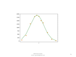
- 76. 76 Abhijit Kar Gupta, email: kg.abhi@gmail.com
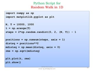
- 77. Random Walk in 1D >>> import numpy as np >>> N, T = 10000, 1000 >>> t = np.arange(T) >>> steps = 2*np.random.randint(0, 2, (N, T)) – 1 >>> print steps [[ 1 -1 1 ... -1 1 -1] [-1 1 1 ... 1 -1 -1] [-1 -1 -1 ... -1 1 1] ... [ 1 -1 1 ... 1 -1 1] [-1 -1 -1 ... -1 1 -1] [ 1 1 1 ... -1 -1 -1]] 77 Abhijit Kar Gupta, email: kg.abhi@gmail.com
- 78. Random walk in 1D (Contn…) >>> positions = np.cumsum(steps, axis = 1) >>> print positions [[ 1 0 1 ... 8 9 8] [ -1 0 1 ... -6 -7 -8] [ -1 -2 -3 ... -22 -21 -20] ... [ 1 0 1 ... -26 -27 -26] [ -1 -2 -3 ... -88 -87 -88] [ 1 2 3 ... -52 -53 -54]] >>> distsq = positions**2 >>> mdistsq = np.mean(distsq, axis = 0) >>> print mdistsq[:10] [ 1. 1.9856 2.9608 3.8988 4.9224 5.8972 6.948 8.1308 9.1472 10.216 ] 78 Abhijit Kar Gupta, email: kg.abhi@gmail.com
- 79. Python Script for Random Walk in 1D import numpy as np import matplotlib.pyplot as plt N, T = 10000, 1000 t = np.arange(T) steps = 2*np.random.randint(0, 2, (N, T)) - 1 positions = np.cumsum(steps, axis = 1) distsq = positions**2 mdistsq = np.mean(distsq, axis = 0) rms = np.sqrt(mdistsq) plt.plot(t, rms) plt.show() 79 Abhijit Kar Gupta, email: kg.abhi@gmail.com
- 80. 80 Abhijit Kar Gupta, email: kg.abhi@gmail.com
- 81. To extract exponent t = np.log(t[10:-1:50]) rms = np.log(rms[10:-1:50]) import numpy.polynomial.polynomial as poly coeffs = poly.polyfit(t, rms, 1) rmsfit = pol.polyval(t, coeffs) print coeffs plt.plot(t, rms, ‘o’, t, rmsfit, ‘-’) plt.xlabel(‘log(time)’) plt.ylabel(‘log(rms-dist)’) plt.show() 81 Abhijit Kar Gupta, email: kg.abhi@gmail.com
- 82. Coeffs: [0.05229699 0.49110655] 82 Abhijit Kar Gupta, email: kg.abhi@gmail.com
- 83. More towards Data Science… 83 Abhijit Kar Gupta, email: kg.abhi@gmail.com
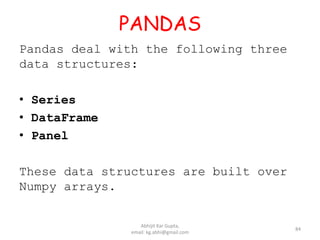
- 84. PANDAS Pandas deal with the following three data structures: • Series • DataFrame • Panel These data structures are built over Numpy arrays. 84 Abhijit Kar Gupta, email: kg.abhi@gmail.com
- 85. Series >>> import pandas as pd >>> import numpy as np >>> x = np.arange(10,50,10) >>> pd.Series(x) 0 10 1 20 2 30 3 40 dtype: int32 85 Abhijit Kar Gupta, email: kg.abhi@gmail.com
- 86. >>> index = ['a', 'b', 'c', 'd'] >>> pd.Series(x, index) a 10 b 20 c 30 d 40 dtype: int32 >>> s = pd.Series(x, index) >>> s[0] 10 >>> s[‘a’] 10 86 Abhijit Kar Gupta, email: kg.abhi@gmail.com
- 87. Series: Methods >>> s.axes [RangeIndex(start=0, stop=4, step=1)] >>> s.values array([10, 20, 30, 40], dtype=int64) >>> s.size 4 >>> s.shape (4,) >>> s.ndim 1 >>> s.dtype dtype('int64') 87 Abhijit Kar Gupta, email: kg.abhi@gmail.com
- 88. >>> s['e'] = 50 >>> s a 10 b 20 c 30 d 40 e 50 dtype: int64 >>> data =['a', 'b', 'c', 'd'] >>> pd.Series(data) 0 a 1 b 2 c 3 d dtype: object 88 Abhijit Kar Gupta, email: kg.abhi@gmail.com
- 89. # Data as scalar >>> index = [‘a’, ‘b’, ‘c’, ‘d’] >>> pd.Series(10, index, int) a 10 b 10 c 10 d 10 dtype: int32 89 Abhijit Kar Gupta, email: kg.abhi@gmail.com
- 90. Series from Dictionary >>> data = {'a':10, 'b':20, 'c':30, 'd':40} >>> pd.Series(data) a 10 b 20 c 30 d 40 dtype: int64 >>> index = ['a', 'b', 'c', 'd', 'e', 'f'] >>> pd.Series(data, index) a 10.0 b 20.0 c 30.0 d 40.0 e NaN f NaN dtype: float64 90 Abhijit Kar Gupta, email: kg.abhi@gmail.com
- 91. Arithmetic operations on Series >>> s a 10 b 20 c 30 d 40 e 50 >>> s*2 a 20 b 40 c 60 d 80 e 100 >>> np.sqrt(s) a 3.162278 b 4.472136 c 5.477226 d 6.324555 e 7.071068 dtype: float64 91 Abhijit Kar Gupta, email: kg.abhi@gmail.com
- 92. >>> sum(s) 150L >>> min(s) 10L >>> max(s) 50L >>> s[1:4] b 20 c 30 d 40 dtype: int64 >>> s.sum() 100 >>> s.mean() 25.0 >>> s.std() 12.909944487358056 92 Abhijit Kar Gupta, email: kg.abhi@gmail.com
- 93. DataFrame >>> x = [10,20,30,40] >>> pd.DataFrame(x) 0 0 10 1 20 2 30 3 40 >>> x = [[10,20,30,40], [50,60,70,80]] >>> pd.DataFrame(x) 0 1 2 3 0 10 20 30 40 1 50 60 70 80 93 Abhijit Kar Gupta, email: kg.abhi@gmail.com
- 94. >>> index = ['a','b'] >>> pd.DataFrame(x, index) 0 1 2 3 a 10 20 30 40 b 50 60 70 80 >>> d = pd.DataFrame(x,index,columns = ['A', 'B', 'C', 'D']) A B C D a 10 20 30 40 b 50 60 70 80 94 Abhijit Kar Gupta, email: kg.abhi@gmail.com
- 95. >>> d[‘A’] a 10 b 50 >>> d[‘A’][‘a’] 10 95 Abhijit Kar Gupta, email: kg.abhi@gmail.com
- 96. Methods over DataFrame • d.axes • d.size • d.ndim • d.T • d.empty • d.values • d.head(1) • d.tail(1) • d.sum() • d.sum(1) • d.mean() • d.mean(1)[1] • d.std() • d.std(1) • d.max() • d.min() • d.describe() # Full Statistics 96 Abhijit Kar Gupta, email: kg.abhi@gmail.com
- 97. DataFrame from the list of Dictionaries >>> data = [{'x':2, 'y':10},{'x':4, 'y':20},{'x':6, 'y':30},{'x':8, 'y':40}] >>> d = pd.DataFrame(data, index=[‘a’,’b’,’c’,’d’]) x y a 2 10 b 4 20 c 6 30 d 8 40 >>> d['x'] a 2 b 4 c 6 d 8 Name: x, dtype: int64 >>> d['x'][‘b’] 4 97 Abhijit Kar Gupta, email: kg.abhi@gmail.com
- 98. DataFrame from Dictionary of Series >>> index = ['a','b','c','d'] >>> s1 = pd.Series([10,20,30,40],index) >>> s2 = pd.Series([100,200,300,400],index) >>> d = {'A':s1, 'B':s2} >>> pd.DataFrame(d) A B a 10 100 b 20 200 c 30 300 d 40 400 >>> D = pd.DataFrame(d) >>> D['A'] a 10 b 20 c 30 d 40 Name: A, dtype: int64 98 Abhijit Kar Gupta, email: kg.abhi@gmail.com
- 99. Add column to DataFrame >>> D['C']= pd.DataFrame({'C':pd.Series([1000,2000,3000,4000],index)}) >>> D A B C a 10 100 1000 b 20 200 2000 c 30 300 3000 d 40 400 4000 >>> D['C'] = pd.DataFrame(pd.Series([1000,2000,3000,4000],index)) >>> D A B C a 10 100 1000 b 20 200 2000 c 30 300 3000 d 40 400 4000 >>> D['C'] = pd.Series([1000,2000,3000,4000],index) >>> D A B C a 10 100 1000 b 20 200 2000 c 30 300 3000 d 40 400 4000 99 Abhijit Kar Gupta, email: kg.abhi@gmail.com
- 100. Delete column and rows from DataFrame >>> D A B C a 10 100 1000 b 20 200 2000 c 30 300 3000 d 40 400 4000 >>> del D['A'] >>> D B C a 100 1000 b 200 2000 c 300 3000 d 400 4000 100 Abhijit Kar Gupta, email: kg.abhi@gmail.com
- 101. Slicing >>> D.loc['b'] A 20 B 200 C 2000 >>> D.iloc[1] A 20 B 200 C 2000 Name: b, dtype: int64 >>> D[1:3] A B C b 20 200 2000 c 30 300 3000 >>> D[1:3]['A'] b 20 c 30 Name: A, dtype: int64 101 Abhijit Kar Gupta, email: kg.abhi@gmail.com
- 102. Append, Delete >>> D1 = pd.DataFrame([[50,500,5000]], index = ['e'],columns=['A','B','C']) >>> D1 A B C e 50 500 5000 >>> D.append(D1) # Append another DataFrame A B C a 10 100 1000 b 20 200 2000 c 30 300 3000 d 40 400 4000 e 50 500 5000 >>> D.drop('a’) # Delete the indexed row. A B C b 20 200 2000 c 30 300 3000 d 40 400 4000 102 Abhijit Kar Gupta, email: kg.abhi@gmail.com
- 103. Re-indexing >>> index = np.arange(1,6) >>> d = pd.DataFrame(data, index, columns = ['x', 'y']) >>> d x y 1 0.1 0.2 2 0.3 0.4 3 0.5 0.6 4 0.7 0.8 5 0.9 1.0 >>> d.reindex(np.arange(2,7), ['x','y']) x y 2 0.3 0.4 3 0.5 0.6 4 0.7 0.8 5 0.9 1.0 6 NaN NaN 103 Abhijit Kar Gupta, email: kg.abhi@gmail.com
- 104. Alignment of two DataFrames by reindexing >>> data = np.random.rand(10,3) >>> d1 = pd.DataFrame(data, index = range(1,11), columns = ['x','y','z']) >>> d1 x y z 1 0.342091 0.044060 0.773249 2 0.934012 0.038944 0.237909 3 0.670108 0.011794 0.831526 4 0.354686 0.381140 0.493882 5 0.690489 0.622695 0.409091 6 0.352255 0.205635 0.551726 7 0.371473 0.392713 0.853915 8 0.601222 0.353043 0.726287 9 0.933808 0.104148 0.718498 10 0.225576 0.812473 0.158370 104 Abhijit Kar Gupta, email: kg.abhi@gmail.com
- 105. >>> data = np.random.rand(8,3) >>> d2 = pd.DataFrame(data, index = range(1,9), columns = ['x','y','z']) >>> d2 x y z 1 0.322780 0.376841 0.957168 2 0.892635 0.248012 0.705469 3 0.006545 0.050196 0.112410 4 0.886808 0.437421 0.658757 5 0.628429 0.961192 0.190440 6 0.374883 0.450280 0.983127 7 0.257246 0.776551 0.425495 8 0.939035 0.471483 0.810289 105 Abhijit Kar Gupta, email: kg.abhi@gmail.com
- 106. >>> d2 = d1.reindex_like(d1) >>> d2 x y z 1 0.342091 0.044060 0.773249 2 0.934012 0.038944 0.237909 3 0.670108 0.011794 0.831526 4 0.354686 0.381140 0.493882 5 0.690489 0.622695 0.409091 6 0.352255 0.205635 0.551726 7 0.371473 0.392713 0.853915 8 0.601222 0.353043 0.726287 9 0.933808 0.104148 0.718498 10 0.225576 0.812473 0.158370 106 Abhijit Kar Gupta, email: kg.abhi@gmail.com
- 107. Panel Panel is a 3D Container. DataFrame is a 2D container. Series is 1D. >>> data = np.random.rand(2,3,4) >>> np.random.rand(2,3,4) array([[[0.05925325, 0.7165947 , 0.34978631, 0.68598632], [0.51410651, 0.50950708, 0.99801304, 0.34533087], [0.75854214, 0.50619351, 0.17673772, 0.4866736 ]], [[0.49319432, 0.03183697, 0.61576345, 0.73591557], [0.41456184, 0.20290885, 0.27732744, 0.63533898], [0.64958528, 0.42573291, 0.13674149, 0.10115889]]]) >>> p = pd.Panel(data) >>> p <class 'pandas.core.panel.Panel'> Dimensions: 2 (items) x 3 (major_axis) x 4 (minor_axis) Items axis: 0 to 1 Major_axis axis: 0 to 2 Minor_axis axis: 0 to 3 107 Abhijit Kar Gupta, email: kg.abhi@gmail.com
- 108. >>> p.major_xs(0) 0 1 0 0.483434 0.126538 1 0.061099 0.254202 2 0.754853 0.631093 3 0.298432 0.573099 >>> p.minor_xs(1) 0 1 0 0.061099 0.254202 1 0.916231 0.034463 2 0.228343 0.853884 108 Abhijit Kar Gupta, email: kg.abhi@gmail.com
- 109. >>> index = ['a','b','c'] >>> data = {'A': pd.DataFrame(np.random.rand(3,4),index), 'B':pd.DataFrame(np.random.rand(3,4),index)} >>> p = pd.Panel(data) >>> p <class 'pandas.core.panel.Panel'> Dimensions: 2 (items) x 3 (major_axis) x 4 (minor_axis) Items axis: A to B Major_axis axis: a to c Minor_axis axis: 0 to 3 109 Abhijit Kar Gupta, email: kg.abhi@gmail.com
- 110. >>> p.major_xs('a') A B 0 0.422049 0.684155 1 0.922664 0.411938 2 0.644187 0.246746 3 0.213998 0.431654 >>> p.minor_xs(1) A B a 0.922664 0.411938 b 0.906779 0.573952 c 0.879191 0.233360 110 Abhijit Kar Gupta, email: kg.abhi@gmail.com
- 111. Methods on Panel >>> p.values array([[[0.42204928, 0.92266448, 0.64418741, 0.21399842], [0.42902311, 0.90677907, 0.67544671, 0.60858596], [0.35946858, 0.87919109, 0.16145494, 0.46737675]], [[0.68415499, 0.411938 , 0.24674607, 0.43165447], [0.15053089, 0.57395153, 0.65095238, 0.7393423 ], >>> p.axes [Index([u'A', u'B'], dtype='object'), Index([u'a', u'b', u'c'], dtype='object'), RangeIndex(start=0, stop=4, step=1)] >>> p.size 24 >>> p.ndim 3 >>> p.shape (2, 3, 4) 111 Abhijit Kar Gupta, email: kg.abhi@gmail.com
- 112. >>> p.sum(1) A B 0 1.210541 1.153222 1 2.708635 1.219250 2 1.481089 1.471627 3 1.289961 1.396990 >>> p.sum(2) A B a 2.202900 1.774494 b 2.619835 2.114777 c 1.867491 1.351817 112 Abhijit Kar Gupta, email: kg.abhi@gmail.com
- 113. Thank you! 113 Abhijit Kar Gupta, email: kg.abhi@gmail.com