Introduction to MatLab programming
Download as PPT, PDF9 likes4,721 views

This document provides an introduction and overview of MATLAB (Matrix Laboratory), an interactive program for numerical computation and visualization. It discusses basic MATLAB commands and functions for creating variables and matrices, performing mathematical operations, plotting graphs, and working with polynomials.


![Entering Matrices (1) >> A = [1 2 3; 4 5 6; 7 8 9] OR >> A = [ 1 2 3 4 5 6 7 8 9 ]](https://image.slidesharecdn.com/matlabnotes-110104184012-phpapp01/85/Introduction-to-MatLab-programming-12-320.jpg)

![Complex Matrices To enter a complex matrix, you may do it in one of two ways : >> A = [1 2; 3 4] + i*[5 6;7 8] OR >> A = [1+5i 2+6i; 3+7i 4+8i]](https://image.slidesharecdn.com/matlabnotes-110104184012-phpapp01/85/Introduction-to-MatLab-programming-15-320.jpg)

![Matrix Addition » A = [ 1 1 1 ; 2 2 2 ; 3 3 3] » B = [3 3 3 ; 4 4 4 ; 5 5 5 ] » A + B ans = 4 4 4 6 6 6 8 8 8](https://image.slidesharecdn.com/matlabnotes-110104184012-phpapp01/85/Introduction-to-MatLab-programming-17-320.jpg)
![Matrix Subtraction » A = [ 1 1 1 ; 2 2 2 ; 3 3 3] » B = [3 3 3 ; 4 4 4 ; 5 5 5 ] » B - A ans = 2 2 2 2 2 2 2 2 2](https://image.slidesharecdn.com/matlabnotes-110104184012-phpapp01/85/Introduction-to-MatLab-programming-18-320.jpg)
![Matrix Multiplication » A = [ 1 1 1 ; 2 2 2 ; 3 3 3] » B = [3 3 3 ; 4 4 4 ; 5 5 5 ] » A * B ans = 12 12 12 24 24 24 36 36 36](https://image.slidesharecdn.com/matlabnotes-110104184012-phpapp01/85/Introduction-to-MatLab-programming-19-320.jpg)


![Concatenation To create a large matrix from a group of smaller ones try A = magic(3) B = [ A, zeros(3,2) ; zeros(2,3), eye(2)] C = [A A+32 ; A+48 A+16] Try some of your own !!](https://image.slidesharecdn.com/matlabnotes-110104184012-phpapp01/85/Introduction-to-MatLab-programming-35-320.jpg)


![Deleting Rows and Columns (1) Create a temporary matrix X X=A; X(:, 2) = [] Deleting a single element won’t result in a matrix, so the following will return an error X(1,2) = []](https://image.slidesharecdn.com/matlabnotes-110104184012-phpapp01/85/Introduction-to-MatLab-programming-42-320.jpg)
![Deleting Rows and Columns (2) However, using a single subscript, you can delete a single element sequence of elements So X(2:2:10) = [] gives x = 16 9 2 7 13 12 1](https://image.slidesharecdn.com/matlabnotes-110104184012-phpapp01/85/Introduction-to-MatLab-programming-43-320.jpg)

![The ‘FIND’ Command (2) A = [ 1 2 3 ; 4 5 6 ; 7 8 9] [i, j] = find (A > 5) i = 3 3 2 3 j = 1 2 3 3](https://image.slidesharecdn.com/matlabnotes-110104184012-phpapp01/85/Introduction-to-MatLab-programming-45-320.jpg)


![The ‘PLOT’ Command (2) >> W = [Y ; Z] >> plot (X,W) Rotate by 90 degrees >> plot(W,X)](https://image.slidesharecdn.com/matlabnotes-110104184012-phpapp01/85/Introduction-to-MatLab-programming-49-320.jpg)


![The ‘PLOT’ Command (2) >> W = [Y ; Z] >> plot (X,W) Rotate by 90 degrees >> plot(W,X)](https://image.slidesharecdn.com/matlabnotes-110104184012-phpapp01/85/Introduction-to-MatLab-programming-52-320.jpg)


![Polynomials Polynomials are represented as row vectors with its coefficients in descending order, e.g. X 4 - 12X 3 + 0X 2 +25X + 116 p = [1 -12 0 25 116]](https://image.slidesharecdn.com/matlabnotes-110104184012-phpapp01/85/Introduction-to-MatLab-programming-57-320.jpg)


![Polynomial Addition/Sub a = [1 2 3 4] b = [1 4 9 16] c = a + b d = b - a](https://image.slidesharecdn.com/matlabnotes-110104184012-phpapp01/85/Introduction-to-MatLab-programming-60-320.jpg)
![Polynomial Addition/Sub What if two polynomials of different order ? X 3 + 2X 2 +3X + 4 X 6 + 6X 5 + 20X 4 - 52X 3 + 81X 2 +96X + 84 a = [1 2 3 4] e = [1 6 20 52 81 96 84] f = e + [0 0 0 a] or f = e + [zeros(1,3) a]](https://image.slidesharecdn.com/matlabnotes-110104184012-phpapp01/85/Introduction-to-MatLab-programming-61-320.jpg)
![Polynomial Multiplication a = [1 2 3 4] b = [1 4 9 16] Perform the convolution of two arrays ! g = conv(a,b) g = 1 6 20 50 75 84 64](https://image.slidesharecdn.com/matlabnotes-110104184012-phpapp01/85/Introduction-to-MatLab-programming-62-320.jpg)
![Polynomial Division a = [1 2 3 4] g = [1 6 20 50 75 84 64] Perform the deconvolution of two arrays ! [q,r] = deconv(g, a) q = {quotient} 1 4 9 16 r = {remainder} 0 0 0 0 0 0 0 0](https://image.slidesharecdn.com/matlabnotes-110104184012-phpapp01/85/Introduction-to-MatLab-programming-63-320.jpg)
![Polynomial Differentiation f = [1 6 20 48 69 72 44] h = polyder(f) h = 6 30 80 144 138 72](https://image.slidesharecdn.com/matlabnotes-110104184012-phpapp01/85/Introduction-to-MatLab-programming-64-320.jpg)
![Polynomial Evaluation x = linspace(-1,3) p = [1 4 -7 -10] v = polyval(p,x) plot (x,v), title(‘Graph of P’)](https://image.slidesharecdn.com/matlabnotes-110104184012-phpapp01/85/Introduction-to-MatLab-programming-65-320.jpg)


![Symbolic Expressions ‘ 1/(2*x^n)’ cos(x^2) - sin(x^2) M = sym(‘[a , b ; c , d]’) f = int(‘x^3 / sqrt(1 - x)’, ‘a’, ‘b’)](https://image.slidesharecdn.com/matlabnotes-110104184012-phpapp01/85/Introduction-to-MatLab-programming-71-320.jpg)


![M-Files To store your own MatLab commands in a file, create it as a text file and save it with a name that ends with “.m” So mymatrix.m A = [… 16.0 3.0 2.0 13.0 5.0 10.0 11.0 8.0 9.0 6.0 7.0 12.0 4.0 15.0 14.0 1.0]; type mymatrix](https://image.slidesharecdn.com/matlabnotes-110104184012-phpapp01/85/Introduction-to-MatLab-programming-83-320.jpg)


![Quick Answer (!) function c = mypoly(a,b) % MYPOLY Add two polynomials of variable lengths % mypoly(a,b) add the polynomial A to the polynomial % B, even if they are of different length % % Author: Damian Gordon % Date : 3/5/2001 % Mod'd : x/x/2001 % c = [zeros(1,length(b) - length(a)) a] + [zeros(1, length(a) - length(b)) b];](https://image.slidesharecdn.com/matlabnotes-110104184012-phpapp01/85/Introduction-to-MatLab-programming-93-320.jpg)


![Curve Fitting Example x = [0 .1 .2 .3 .4 .5 .6 .7 .8 .9 1]; y = [-.447 1.978 3.28 6.16 7.08 7.34 7.66 9.56 9.48 9.30 11.2]; polyfit(x,y,n) n = 1 p = 10.3185 1.4400 n = 2 p = -9.8108 20.1293 -0.0317 y = -9.8108x 2 + 20.1293x - 0.0317](https://image.slidesharecdn.com/matlabnotes-110104184012-phpapp01/85/Introduction-to-MatLab-programming-97-320.jpg)


Introduction to MatLab programming
- 1. Zen and the Art of MatLab Damian Gordon
- 2. Hard work done by : Daphne Gilbert & Susan Lazarus
- 3. Introduction to MatLab MatLab is an interactive, matrix-based system for numeric computation and visualisation MATrix LABoratory Used in image processing, image synthesis, engineering simulation, etc.
- 4. References “ Mastering MatLab” Duane Hanselman, Bruce Littlefield “ The MatLab Primer” http://www.fi.uib.no/Fysisk/Teori/KURS/WRK/mat/mat.html “ The MatLab FAQ” http://www.isr.umd.edu/~austin/ence202.d/matlab-faq.html
- 8. MATLAB Command Window To get started, type one of these: helpwin, helpdesk, or demo. For product information, type tour or visit www.mathworks.com. » » help HELP topics:
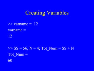
- 9. Creating Variables >> varname = 12 varname = 12 >> SS = 56; N = 4; Tot_Num = SS + N Tot_Num = 60
- 10. Operations + Addition - Subtraction * Multiplication ^ Power \ Division / Division Add vars Subtract vars Multiplication Raise to the power Divide vars (A div B) Divide vars (B div A)
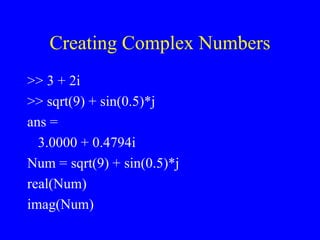
- 11. Creating Complex Numbers >> 3 + 2i >> sqrt(9) + sin(0.5)*j ans = 3.0000 + 0.4794i Num = sqrt(9) + sin(0.5)*j real(Num) imag(Num)
- 12. Entering Matrices (1) >> A = [1 2 3; 4 5 6; 7 8 9] OR >> A = [ 1 2 3 4 5 6 7 8 9 ]
- 13. Entering Matrices (2) To create an NxM zero-filled matrix >> zeros(N,M) To create a NxN zero-filled matrix >> zeros(N) To create an NxM one-filled matrix >> ones(N,M) To create a NxN one-filled matrix >> ones(N)
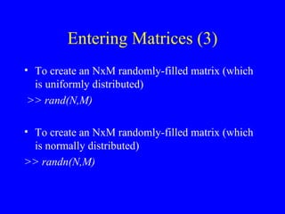
- 14. Entering Matrices (3) To create an NxM randomly-filled matrix (which is uniformly distributed) >> rand(N,M) To create an NxM randomly-filled matrix (which is normally distributed) >> randn(N,M)
- 15. Complex Matrices To enter a complex matrix, you may do it in one of two ways : >> A = [1 2; 3 4] + i*[5 6;7 8] OR >> A = [1+5i 2+6i; 3+7i 4+8i]
- 16. MATLAB Command Window » who Your variables are: a b c » whos Name Size Bytes Class a 8x8 512 double array b 9x9 648 double array c 9x9 648 double array Grand total is 226 elements using 1808 bytes
- 17. Matrix Addition » A = [ 1 1 1 ; 2 2 2 ; 3 3 3] » B = [3 3 3 ; 4 4 4 ; 5 5 5 ] » A + B ans = 4 4 4 6 6 6 8 8 8
- 18. Matrix Subtraction » A = [ 1 1 1 ; 2 2 2 ; 3 3 3] » B = [3 3 3 ; 4 4 4 ; 5 5 5 ] » B - A ans = 2 2 2 2 2 2 2 2 2
- 19. Matrix Multiplication » A = [ 1 1 1 ; 2 2 2 ; 3 3 3] » B = [3 3 3 ; 4 4 4 ; 5 5 5 ] » A * B ans = 12 12 12 24 24 24 36 36 36
- 20. Matrix - Power » A ^ 2 ans = 6 6 6 12 12 12 18 18 18 » A ^ 3 ans = 36 36 36 72 72 72 108 108 108
- 21. Matrix Transpose A = 1 1 1 2 2 2 3 3 3 » A' ans = 1 2 3 1 2 3 1 2 3
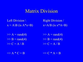
- 22. Matrix Division Left Division \ x = A\B (is A*x=B) >> A = rand(4) >> B = rand(4) >> C = A \ B => A * C = B Right Division / x=A/B (is x*A=B) >> A = rand(4) >> B = rand(4) >> C = A / B => C * A = B
- 23. Matrix Operations + Addition - Subtraction * Multiplication ^ Power ‘ Conjugate Transpose \ Left Division / Right Division Add matrices Subtract matrices Matrix Multiplication Raise to the power Get transpose x = A\B (is A*x=B) x=A/B (is x*A=B)
- 24. Philosophiae Naturalis Principia Matlab ematica Damian Gordon
- 26. Magic Matrix MAGIC Magic square. MAGIC(N) is an N-by-N matrix constructed from the integers 1 through N^2 with equal row, column, and diagonal sums. Produces valid magic squares for N = 1,3,4,5,...
- 27. Identity Function >> eye (4) ans = 1 0 0 0 0 1 0 0 0 0 1 0 0 0 0 1
- 28. Upper Triangle Matrix » a = ones(5) a = 1 1 1 1 1 1 1 1 1 1 1 1 1 1 1 1 1 1 1 1 1 1 1 1 1 » triu(a) ans = 1 1 1 1 1 0 1 1 1 1 0 0 1 1 1 0 0 0 1 1 0 0 0 0 1
- 29. Lower Triangle Matrix » a = ones(5) a = 1 1 1 1 1 1 1 1 1 1 1 1 1 1 1 1 1 1 1 1 1 1 1 1 1 » tril(a) ans = 1 0 0 0 0 1 1 0 0 0 1 1 1 0 0 1 1 1 1 0 1 1 1 1 1
- 30. Hilbert Matrix » hilb(4) ans = 1.0000 0.5000 0.3333 0.2500 0.5000 0.3333 0.2500 0.2000 0.3333 0.2500 0.2000 0.1667 0.2500 0.2000 0.1667 0.1429
- 31. Inverse Hilbert Matrix » invhilb(4) ans = 16 -120 240 -140 -120 1200 -2700 1680 240 -2700 6480 -4200 -140 1680 -4200 2800
- 32. Toeplitz matrix. TOEPLITZ TOEPLITZ(C,R) is a non-symmetric Toeplitz matrix having C as its first column and R as its first row. TOEPLITZ(R) is a symmetric (or Hermitian) Toeplitz matrix. -> See also HANKEL
- 33. Summary of Functions magic eye(4) triu(4) tril(4) hilb(4) invhilb(4) toeplitz(4) - magic matrix - identity matrix - upper triangle - lower triangle - hilbert matrix - Inverse Hilbert matrix - non-symmetric Toeplitz matrix
- 34. Dot Operator A = magic(4); b=ones(4); A * B A.*B the dot operator performs element-by-element operations, for “*”, “\” and “/”
- 35. Concatenation To create a large matrix from a group of smaller ones try A = magic(3) B = [ A, zeros(3,2) ; zeros(2,3), eye(2)] C = [A A+32 ; A+48 A+16] Try some of your own !!
- 36. Subscripts Row i and Column j of matrix A is denoted by A(i,j) A = Magic(4) try A(1,4) + A(2,4) + A(3,4) + A(4,4) try A(4,5)
- 37. The Colon Operator (1) This is one MatLab’s most important operators 1:10 means the vector 1 2 3 4 5 6 7 8 9 10 100:-7:50 100 93 86 79 72 65 58 51 0:pi/4:pi 0 0.7854 1.5708 2.3562 3.1416
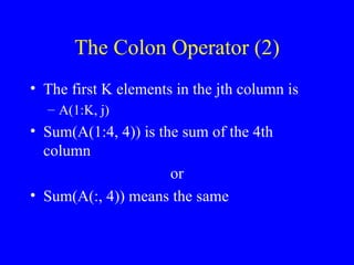
- 38. The Colon Operator (2) The first K elements in the jth column is A(1:K, j) Sum(A(1:4, 4)) is the sum of the 4th column or Sum(A(:, 4)) means the same
- 39. matlABBA
- 40. The Colon Operator (1) This is one MatLab’s most important operators 1:10 means the vector 1 2 3 4 5 6 7 8 9 10 100:-7:50 100 93 86 79 72 65 58 51 0:pi/4:pi 0 0.7854 1.5708 2.3562 3.1416
- 41. The Colon Operator (2) The first K elements in the jth column is A(1:K, j) Sum(A(1:4, 4)) is the sum of the 4th column or Sum(A(:, 4)) means the same
- 42. Deleting Rows and Columns (1) Create a temporary matrix X X=A; X(:, 2) = [] Deleting a single element won’t result in a matrix, so the following will return an error X(1,2) = []
- 43. Deleting Rows and Columns (2) However, using a single subscript, you can delete a single element sequence of elements So X(2:2:10) = [] gives x = 16 9 2 7 13 12 1
- 44. The ‘FIND’ Command (1) >> x = -3:3 x = -3 -2 -1 0 1 2 3 K = find(abs(x) > 1) K = 1 2 6 7
- 45. The ‘FIND’ Command (2) A = [ 1 2 3 ; 4 5 6 ; 7 8 9] [i, j] = find (A > 5) i = 3 3 2 3 j = 1 2 3 3
- 46. Special Variables ans pi eps flops inf NaN i,j why - default name for results - pi - “help eps” - count floating point ops - Infinity, e.g. 1/0 - Not a number, e.g. 0/0 - root minus one - why not ?
- 47. LOGO Command
- 48. The ‘PLOT’ Command (1) >> X = linspace(0, 2*pi, 30); >> Y = sin(X); >> plot(X,Y) >> Z = cos(X); >> plot(X,Y,X,Z);
- 49. The ‘PLOT’ Command (2) >> W = [Y ; Z] >> plot (X,W) Rotate by 90 degrees >> plot(W,X)
- 51. The ‘PLOT’ Command (1) >> X = linspace(0, 2*pi, 30); >> Y = sin(X); >> plot(X,Y) >> Z = cos(X); >> plot(X,Y,X,Z);
- 52. The ‘PLOT’ Command (2) >> W = [Y ; Z] >> plot (X,W) Rotate by 90 degrees >> plot(W,X)
- 53. PLOT Options >> plot(X,Y,’g:’) >> plot(X,Y,’r-’) >> plot(X,Y,’ko’) >> plot(X,Y,’g:’,X,Z,’r-’,X,Y,’wo’,X,Z,’c+’);
- 54. PLOT Options >> grid on >> grid off >> xlabel(‘this is the x axis’); >> ylabel(‘this is the y axis’); >> title(‘Title of Graph’); >> text(2.5, 0.7, ’sin(x)’); >> legend(‘sin(x)’, ‘cos(x)’)
- 55. SUBPLOT Command Subplot(m,n,p) creates a m-by-n matrix in and plots in the p th plane. subplot(2,2,1) plot(X,Y) subplot(2,2,2) plot(X,Z) subplot(2,2,3) plot( X,Y,X,Z) subplot(2,2,4) plot(W,X)
- 56. Specialised matrices compan gallery hadamard hankel pascal rosser vander wilkinson Companion matrix Higham test matrices Hadamard matrix Hankel matrix Pascal matrix. Classic symmetric eigenvalue test problem Vandermonde matrix Wilkinson's eigenvalue test matrix
- 57. Polynomials Polynomials are represented as row vectors with its coefficients in descending order, e.g. X 4 - 12X 3 + 0X 2 +25X + 116 p = [1 -12 0 25 116]
- 58. Polynomials The roots of a polynomial are found as follows r = roots(p) roots are represented as a column vector
- 59. Polynomials Generating a polynomial from its roots polyans = poly(r) includes imaginary bits due to rounding mypolyans = real(polyans)
- 60. Polynomial Addition/Sub a = [1 2 3 4] b = [1 4 9 16] c = a + b d = b - a
- 61. Polynomial Addition/Sub What if two polynomials of different order ? X 3 + 2X 2 +3X + 4 X 6 + 6X 5 + 20X 4 - 52X 3 + 81X 2 +96X + 84 a = [1 2 3 4] e = [1 6 20 52 81 96 84] f = e + [0 0 0 a] or f = e + [zeros(1,3) a]
- 62. Polynomial Multiplication a = [1 2 3 4] b = [1 4 9 16] Perform the convolution of two arrays ! g = conv(a,b) g = 1 6 20 50 75 84 64
- 63. Polynomial Division a = [1 2 3 4] g = [1 6 20 50 75 84 64] Perform the deconvolution of two arrays ! [q,r] = deconv(g, a) q = {quotient} 1 4 9 16 r = {remainder} 0 0 0 0 0 0 0 0
- 64. Polynomial Differentiation f = [1 6 20 48 69 72 44] h = polyder(f) h = 6 30 80 144 138 72
- 65. Polynomial Evaluation x = linspace(-1,3) p = [1 4 -7 -10] v = polyval(p,x) plot (x,v), title(‘Graph of P’)
- 66. Rational Polynomials Rational polynomials, seen in Fourier, Laplace and Z transforms We represent them by their numerator and denominator polynomials we can use residue to perform a partial fraction expansion We can use polyder with two inputs to differentiate rational polynomials
- 67. An Anthropologist on Matlab
- 68. Data Analysis Functions (1) corrcoef(x) cov(x) cplxpair(x) cross(x,y) cumprod(x) cumsum(x) del2(A) diff(x) dot(x,y) gradient(Z, dx, dy) Correlation coefficients Covariance matrix complex conjugate pairs vector cross product cumulative prod of cols cumulative sum of cols five-point discrete Laplacian diff between elements vector dot product approximate gradient
- 69. Data Analysis Functions (2) histogram(x) max(x), max(x,y) mean(x) median(x) min(x), min(x,y) prod(x) sort(x) std(x) subspace(A,B) sum(x) Histogram or bar chart max component mean of cols median of cols minimum component product of elems in col sort cols (ascending) standard dev of cols angle between subspaces sum of elems per col
- 71. Symbolic Expressions ‘ 1/(2*x^n)’ cos(x^2) - sin(x^2) M = sym(‘[a , b ; c , d]’) f = int(‘x^3 / sqrt(1 - x)’, ‘a’, ‘b’)
- 72. Symbolic Expressions diff(‘cos(x)’) ans = -sin(x) det(M) ans = a*d - b * c
- 73. Symbolic Functions numden(m) - num & denom of polynomial symadd(f,g) - add symbolic polynomials symsub(f,g) - sub symbolic polynomials symmul(f,g) - mult symbolic polynomials symdiv(f,g) - div symbolic polynomials sympow(f,’3*x’) - raise f^3
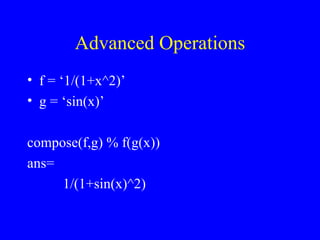
- 74. Advanced Operations f = ‘1/(1+x^2)’ g = ‘sin(x)’ compose(f,g) % f(g(x)) ans= 1/(1+sin(x)^2)
- 75. Advanced Operations finverse(x^2) ans = x^(1/2) symsum(‘(2*n - 1) ^ 2’, 1, ‘n’) ans = 11/3*n + 8/3-4*(n+1)^2 + 4/3*(n+1)^3
- 76. Symbolic Differentiation f = ‘a*x^3 + x^2 + b*x - c’ diff(f) % by default wrt x ans = 3*a^2 + 2*x + b diff(f, ‘a’) % wrt a ans = x^3 diff(f,’a’,2) % double diff wrt a ans = 0
- 77. Symbolic Integration f = sin(s+2*x) int(f) ans = -1/2*cos(s+2*x) int(f,’s’) ans = -cos(s+2*x) int(f, ‘s’, pi/2,pi) ans= -cos(s)
- 78. Comments &Punctuation (1) All text after a percentage sign (%) is ignored >> % this is a comment Multiple commands can be placed on one line separated by commas (,) >> A = magic(4), B = ones(4), C = eye(4)
- 79. Comments &Punctuation (2) A semicolon may be also used, either after a single command or multiple commands >> A = magic(4); B = ones(4); C = eye(4); Ellipses (…) indicate a statement is continued on the next line A = B/… C
- 80. SAVE Command (1) >> save Store all the variables in binary format in a file called matlab.mat >> save fred Store all the variables in binary format in a file called fred.mat >> save a b d fred Store the variables a, b and d in fred.mat
- 81. SAVE Command (2) >> save a b d fred -ascii Stores the variables a, b and d in a file called fred.mat in 8-bit ascii format >> save a b d fred -ascii -double Stores the variables a, b and d in a file called fred.mat in 16-bit ascii format
- 82. Load Command Create a text file called mymatrix.dat with 16.0 3.0 2.0 13.0 5.0 10.0 11.0 8.0 9.0 6.0 7.0 12.0 4.0 15.0 14.0 1.0 “ load mymatrix.dat”, create variable mymatrix
- 83. M-Files To store your own MatLab commands in a file, create it as a text file and save it with a name that ends with “.m” So mymatrix.m A = [… 16.0 3.0 2.0 13.0 5.0 10.0 11.0 8.0 9.0 6.0 7.0 12.0 4.0 15.0 14.0 1.0]; type mymatrix
- 84. IF Condition if condition {commands} end If x = 2 output = ‘x is even’ end
- 85. WHILE Loop while condition {commands} end X = 10; count = 0; while x > 2 x = x / 2; count = count + 1; end
- 86. FOR Loop for x=array {commands} end for n = 1:10 x(n) = sin(n); end A = zeros(5,5); % prealloc for n = 1:5 for m = 5:-1:1 A(n,m) = n^2 + m^2; end disp(n) end
- 87. Creating a function function a = gcd(a,b) % GCD Greatest common divisor % gcd(a,b) is the greatest common divisor of % the integers a and b, not both zero. a = round(abs(a)); b = round(abs(b)); if a == 0 & b == 0 error('The gcd is not defined when both numbers are zero') else while b ~= 0 r = rem(a,b); a = b; b = r; end end
- 88. Quick Exercise (!) Consider Polynomial Addition again : how would you write a program that takes in two polynomials and irrespective of their sizes it adds the polynomials together ? Given that the function length(A) returns the length of a vector. Answers on a postcard to : dgordon@maths.kst.dit.ie oh, and while you’re here anyhow, if you have a browser open, please go to the following sites : http://www.the hungersite.com http://www.hitsagainsthunger.com
- 89. Flash Gordon and the Mud Men of Matlab
- 90. Quick Exercise (!) Consider Polynomial Addition again : how would you write a program that takes in two polynomials and irrespective of their sizes it adds the polynomials together ? Given that the function length(A) returns the length of a vector. Answers on a postcard to : dgordon@maths.kst.dit.ie oh, and while you’re here anyhow, if you have a browser open, please go to the following sites : http://www.the hungersite.com http://www.hitsagainsthunger.com
- 91. Creating Programs Title : Program.m function out = program(inputs) % PROGRAM <code> C:
- 92. Know Thyself Where am I ? pwd Get me onto the hard disk cd C: Where am I now ? pwd Get me to where I know cd ..
- 93. Quick Answer (!) function c = mypoly(a,b) % MYPOLY Add two polynomials of variable lengths % mypoly(a,b) add the polynomial A to the polynomial % B, even if they are of different length % % Author: Damian Gordon % Date : 3/5/2001 % Mod'd : x/x/2001 % c = [zeros(1,length(b) - length(a)) a] + [zeros(1, length(a) - length(b)) b];
- 94. Recursion function b = bart(a) %BART The Bart Simpson program writes on the blackboard % program, Bart writes the message a few times % and then goes home to see the Simpsons if a == 1 disp( 'I will not....'); else disp( 'I will not skateboard in the halls'); bart(a - 1); end
- 95. Curve Fitting What is the best fit ? In this case least squares curve fit What curve should be used ? It depends...
- 96. POLYFIT : Curve Fitting polyfit(x,y,n) - fit a polynomial x,y - data points describing the curve n - polynomial order n = 1 -- linear regression n = 2 -- quadratic regression
- 97. Curve Fitting Example x = [0 .1 .2 .3 .4 .5 .6 .7 .8 .9 1]; y = [-.447 1.978 3.28 6.16 7.08 7.34 7.66 9.56 9.48 9.30 11.2]; polyfit(x,y,n) n = 1 p = 10.3185 1.4400 n = 2 p = -9.8108 20.1293 -0.0317 y = -9.8108x 2 + 20.1293x - 0.0317
- 98. Curve Fitting Example xi = linspace(0,1,100); z = polyval(p,xi) plot(x,y,'o',x,y,xi,z,':');
- 99. Interpolation - 1D t = interp1(x,y,.75) t = 9.5200 also interp1(x,y,.75,’spline’) interp1(x,y,.75,’cubic’)
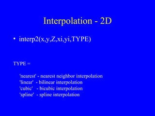
- 100. Interpolation - 2D interp2(x,y,Z,xi,yi,TYPE) TYPE = 'nearest' - nearest neighbor interpolation 'linear' - bilinear interpolation 'cubic' - bicubic interpolation 'spline' - spline interpolation
- 101. Fourier Functions fft fft2 ifft ifft2 filter filter2 fftshift Fast fourier transform 2-D fft Inverse fft 2-D Inverse fft Discrete time filter 2-D discrete tf shift FFT results so -ve freqs appear first
- 102. Tensors See ‘Programs’ ‘ Tensors’ ‘ Tensors.html’
- 103. 3D Graphics T = 0:pi/50:10*pi; plot3(sin(t), cos(t), t);
- 104. 3D Graphics title('Helix'), xlabel('sin(t)'), ylabel('cos(t)'), zlabel('t') grid
- 105. 3D Graphics Rotate view by elevation and azimuth view(az, el); view(-37.5, 60);