SlideShare a Scribd company logo
A Simple Guide to the Analysis of
       Quantitative Data

 An Introduction with hypotheses,
   illustrations and references


                By


       Paul Andrew Bourne
A Simple Guide to the Analysis of
        Quantitative Data: An Introduction with
          hypotheses, illustrations and references


                                          By


                         Paul Andrew Bourne
       Health Research Scientist, the University of the West Indies,
                             Mona Campus


Department of Community Health and Psychiatry
Faculty of Medical Sciences
The University of the West Indies, Mona Campus, Kingston, Jamaica


                                            2
© Paul Andrew Bourne 2009


A Simple Guide to the Analysis of Quantitative Data: An Introduction with hypotheses,
illustrations and references


The copyright of this text is vested in Paul Andrew Bourne and the Department of Community
Health and Psychiatry is the publisher, no chapter may be reproduced wholly or in part without
the expressed permission in writing of both author and publisher.


All rights reserved. Published April, 2009


Department of Community Health and Psychiatry
Faculty of Medical Sciences
The University of the West Indies, Mona Campus, Kingston, Jamaica.


National Library of Jamaica Cataloguing in Publication Data

A catalogue record for this book is available from the National Library of Jamaica

ISBN 978-976-41-0231-1 (pbk)


Covers were designed and photograph taken by Paul Andrew Bourne


                                               3
Table of Contents
                                                                                   Page

Preface                                                                             8
Menu bar – Contents of the Menu bar in SPSS                                        11
              Function - Purposes of the different things on the menu bar          12
Mathematical symbols (numeric operations), in SPSS                                 13
Listing of Other Symbols                                                           14
The whereabouts of some SPSS functions, or commands                                16
Disclaimer                                                                         19
Coding Missing Data                                                                20
Computing Date of Birth                                                            21
List of Figures                                                                    26
List of Tables                                                                     29
How do I obtain access to the SPSS PROGRAM?                                        35
1. INTRODUCTION ……………………………………………………………........                                    43
       1.1.0a: steps in the analysis of hypothesis……………………………………                   45
       1.1.1a Operational definitions of a variable…………………………………                   47
       1.1.1b Typologies of variable ………………..……………………………….                         49
       1.1.1 Levels of measurement………..………………………………………...                          50
       1.1.3 Conceptualizing descriptive and inferential statistics ………………..       59

2. DESCRIPTIVE STATISTICS ANALYZED ….……………………………........                           62
      2.1.1 Interpreting data based on their levels of measurement………..…….         64
      2.1.2 Treating missing (i.e. non-response) cases…………………….……….                84

3. HYPOTHESES: INTRODUCTION …………………………….……………….                                    87
      3.1.1 Definitions of Hypotheses………………..……..……………………….                        88
      3.1.2: Typologies of Hypothesis………………………………………………                            89
      3.1.3: Directional and non-Directional Hypotheses…………………………..                90
      3.1.4 Outliers (i.e. skewness)…………………………….…………………….                          91
      3.1.5 Statistical approaches for treating skewness…………….………………               93

4. Hypothesis 1…[using Cross tabulations and Spearman ranked ordered correlation]
                  ………………………………………………………..                             96

A1.   Physical and social factors and instructional resources will directly influence the
      academic performance of students who will write the Advanced Level Accounting
      Examination;
A2.   Physical and social factors and instructional resources positively influence the
      academic performance of students who write the Advanced level Accounting
      examination and that the relationship varies according to gender;


                                           4
B1.     Pass successes in Mathematics, Principles of Accounts and English Language at the
        Ordinary/CXC General level will positively influence success on the Advanced level
        Accounting examination;
B2.     Pass successes in Mathematics, Principles of Accounts and English Language at the
        Ordinary.

5. Hypothesis 2…………[using Crosstabulations]..…………………………….. 152

        There is a relationship between religiosity, academic performance, age and marijuana
        smoking of Post-primary schools students and does this relationship varies based on
        gender.

6. Hypothesis 3……….…..…[Paired Sample t-test]…….………………………                                    164

        There is a statistical difference between the pre-Test and the post-Test scores.

7. Hypothesis 4….………[using Pearson Product Moment Correlation]…..…........                   184

      Ho: There is no statistical relationship between expenditure on social programmes (public
      expenditure on education and health) and levels of development in a country; and
      H1: There is a statistical association between expenditure on social programmes (i.e.
      public expenditure on education and health) and levels of development in a country

8. Hypothesis 5….. ………[using Logistic Regression]…………………………........                          199

        The health care seeking behaviour of Jamaicans is a function of educational level,
        poverty, union status, illnesses, duration of illnesses, gender, per capita consumption,
        ownership of health insurance policy, and injuries. [ Health Care Seeking Behaviour =
        f( educational levels, poverty, union status, illnesses, duration of illnesses, gender, per
        capita consumption, ownership of health insurance policy, injuries)]

9. Hypothesis 6….. ……[using Linear Regression] ….…………………………..                                207

       There is a negative correlation between access to tertiary level education and
       poverty controlled for sex, age, area of residence, household size, and educational level
of parents

10. Hypothesis 7….. ……[using Pearson Product Moment Correlation Coefficient and
                             Crosstabulations]……………………….......................             223

        There is an association between the introduction of the Inventory Readiness Test and
        the Performance of Students in Grade 1


                                                5
11. Hypothesis 8….…………[using Spearman rho]………………………………....                               232


      The people who perceived themselves to be in the upper class and middle class are
      more so than those in the lower (or working) class do strongly believe that acts of
      incivility are only caused by persons in garrison communities


12. Hypothesis 9………………………………………………………………........                                         235

      Various cross tabulations


13. Hypothesis 10………[using Pearson and Crosstabulations]………………........                   249

      There is no statistical difference between the typology of workers in the   construction
      industry and how they view 10-most top productivity outcomes

14. Hypothesis 11….…[using Crosstabulations and Linear Regression]……........             265

      Determinants of the academic performance of students


15. Hypothesis 12….……[using Spearman ranked ordered correlation]…........                278

      People who perceived themselves to be within the lower social status (i.e. class) are
      more likely to be in-civil than those of the upper classes.

16. Data Transformation…………………………………………………........                                       281

      Recoding                                                                           291
      Dummying variables                                                                 309
      Summing similar variables                                                          331
      Data reduction                                                                     340


Glossary……………..….. ………………………………………………………........                                         350

Reference…..………….…………………………………………………………........                                          352

Appendices…………..….. ………………………………………………………........                                        356
      Appendix 1- Labeling non-responses                                                 356


                                              6
Appendix 2- Statistical errors in data                                                    357
Appendix 3- Research Design                                                               359
Appendix 4- Example of Analysis Plan                                                      366
Appendix 5- Assumptions in regression                                                     367
Appendix 6- Steps in running a bivariate cross tabulation                                 368
Appendix 7- Steps in running a trivariate cross tabulation                                380
Appendix 8- What is placed in a cross tabulations table, using the above SPSS output
                       394
Appendix 9- How to run a Regression in SPSS                                               395
Appendix 10- Running Regression in SPSS                                                   396
Appendix 11a- Interpreting strength of associations                                       407
Appendix 11b - Interpreting strength of association                                       408
Appendix 12- Selecting cases                                                              409
Appendix 13- ‘UNDO’ selecting cases                                                       417
Appendix 14- Weighting cases                                                              420
Appendix 15- ‘Undo’ weighting cases                                                       429
Appendix 15- Statistical symbolisms                                                       440
Appendix 16 – Converting from ‘string’ to ‘numeric’ data –

                 Apparatus One – Converting from string data to numeric data              443

                 Apparatus Two – Converting from alphabetic and numeric data
                                  to all ‘numeric data                                    447

Appendix 17- Steps in running Spearman rho                                                454

Appendix 18- Steps in running Pearson’s Product Moment Correlation                        459

Appendix 19-Sample sizes and their appropriate sampling error                             464

Appendix 20 – Calculating sample size from sampling error(s)                              465

Appendix 21 – Sample sizes and their sampling errors                                      467

Appendix 22 - Sample sizes and their sampling errors                                      468

Appendix 23 – If conditions                                                               469

Appendix 24 – The meaning of ρ value                                                      477

Appendix 25 – Explaining Kurtosis and Skewness                                            478

Appendix 26 – Sampled Research Papers                                                  479-560


                                             7
PREFACE


One of the complexities for many undergraduate students and for first time researchers is ‘How
to blend their socialization with the systematic rigours of scientific inquiry?’ For some, the
socialization process would have embedded in them hunches, faith, family authority and even
‘hearsay’ as acceptable modes of establishing the existence of certain phenomena. These are
not principles or approaches rooted in academic theorizing or critical thinking. Despite
insurmountable scientific evidence that have been gathered by empiricism, the falsification of
some perspectives that students hold are difficulty to change as they still want to hold ‘true’ to
the previous ways of gaining knowledge. Even though time may be clearly showing those
issues are obsolete or even ‘mythological’, students will always adhere to information that they
had garnered in their early socialization. The difficulty in objectivism is not the ‘truths’ that it
claims to provide and/or how we must relate to these realities, it is ‘how do young researchers
abandon their preferred socialization to research findings? Furthermore, the difficulty of
humans and even more so upcoming scholars is how to validate their socialization with
research findings in the presence of empiricism.
        Within the aforementioned background, social researchers must understand that ethic
must govern the reporting of their findings, irrespective of the results and their value systems.
Ethical principles, in the social or natural research, are not ‘good’ because of their inherent
construction, but that they are protectors of the subjects (participants) from the researcher(s)
who may think the study’s contribution is paramount to any harm that the interviewees may
suffer from conducting the study. Then, there is the issue of confidentiality, which sometimes
might be conflicting to the personal situations faced by the researcher. I will be simplistic to
suggest that who takes precedence is based on the code of conduct that guides that profession.
Hence, undergraduate students should be brought into the general awareness that findings must
be reported without any form of alteration. This then give rise to ‘how do we systematically
investigate social phenomena?’

        The aged old discourse of the correctness of quantitative versus qualitative research
will not be explored in this work as such a debate is obsolete and by rehashing this here is a
pointless dialogue. Nevertheless, this textbook will forward illustrations of how to analyze
quantitative data without including any qualitative interpretation techniques. I believe that the
problems faced by students as how to interpret statistical data (ie quantitative data), must be
addressed as the complexities are many and can be overcome in a short time with assistance.

       My rationale for using ‘hypotheses’ as the premise upon which to build an analysis is
embedded in the logicity of how to explore social or natural happenings. I know that
hypothesis testing is not the only approach to examining current germane realities, but that it is
one way which uses more ‘pure’ science techniques than other approaches.

        Hypothesis testing is simply not about null hypothesis, Ho (no statistical relationships),
or alternative hypothesis, Ha, it is a systematic approach to the investigation of observable
phenomenon. In attempting to make undergraduate students recognize the rich annals of
hypothesis testing and how they are paramount to the discovery of social fact, I will

                                                 8
recommend that we begin by reading Thomas S. Kuhn (the Scientific Revolution), Emile
Durkheim (study on suicide), W.E.B. DuBois (study on the Philadelphian Negro) and the
works of Garth Lipps that clearly depict the knowledge base garnered from their usage.

        In writing this book, I tried not to assume that readers have grasped the intricacies of
quantitative data analysis as such I have provided the apparatus and the solutions that are
needed in analyzing data from stated hypotheses. The purpose for this approach is for junior
researchers to thoroughly understand the materials while recognizing the importance of
hypothesis testing in scientific inquiry.


                                            Paul Andrew Bourne, Dip Ed, BSc, MSc, PhD
                                                                        Health Research Scientist
                                     Department of Community Health and Psychiatry
                                                        Faculty of Medical Sciences
                                                   The University of the West Indies
                                                                     Mona-Jamaica.


                                               9
ACKNOWLEDGEMENT


This textbook would not have materialized without the assistance of a number of people
(scholars, associates, and students) who took the time from their busy schedule to guide,
proofread and make invaluable suggestions to the initial manuscript. Some of the individuals
who have offered themselves include Drs. Ikhalfani Solan, Samuel McDaniel and Lawrence
Nicholson who proofread the manuscript and made suggestions as to its appropriateness,
simplicities and reach to those it intend to serve. Furthermore, Mr. Maxwell S. Williams is
very responsible for fermenting the idea in my mind for a book of this nature. Special thanks
must be extended to Mr. Douglas Clarke, an associate, who directed my thoughts in time of
frustration and bewilderment, and on occasions gave me insight on the material and how it
could be made better for the students.

       In addition, I would like to extend my heartiest appreciation to Professor Anthony
Harriott and Dr. Lawrence Powell both of the department of Government, UWI, Mona-
Jamaica, who are my mentors and have provided me with the guidance, scope for the material
and who also offered their expert advice on the initial manuscript.

       Also, I would like to take this opportunity to acknowledge all the students of
Introduction to Political Science (GT24M) of the class 2006/07 who used the introductory
manuscript and made their suggestions for its improvement, in particular Ms. Nina Mighty.


                                             10
Menú Bar


Content:

A social researcher should not only be cognizant of statistical techniques and modalities of
performing his/her discipline, but he/she needs to have a comprehensive grasp of the various
functions within the ‘menu’ of the SPSS program. Where and what are constituted within the
‘menu bar’; and what are the contents’ functions?

                                                                           ‘Menu bar’ contains
                                                                           the following:

                                                                               -   File
                                                                               -   Edit
                                                                               -   View
                                                                               -   Data
                                                                               -   Transform
                                                                               -   Analyze
                                                                               -   Graph
                                                                               -   Utilities
                                                                               -   Add-ons
                                                                               -   Window
                                                                               -   Help


                                The functions of the various contents of the
                                     ‘menu bar’ are explored overleaf


Box 1: Menu Function


                                             11
Menu Bar


Functions: Purposes of the different things on the menu bar


File – This icon deals with the different functions associated with files such as (i) opening ..,
       (ii) reading …, (iii) saving …, (iv) existing.

Edit – This icon stores functions such as – (i) copying, (ii) pasting, (iii) finding, and (iv)
       replacing.

View – Within this lie functions that are screen related.

Data – This icon operates several functions such as – (i) defining, (ii) configuring, (iii)
      entering data, (iv) sorting, (v) merging files, (vi) selecting and weighting cases, and
      (vii) aggregating files.

Transform – Transformation is concerned with previously entered data including (i) recoding,
      (ii) computing, (iii) reordering, and (vi) addressing missing cases.

Analyze – This houses all forms of data analysis apparatus, with a simply click of the Analyze
      command.


Graph – Creation of graphs or charts can begin with a click on Graphs command


Utilities – This deals with sophisticated ways of making complex data operations easier, as
        well as just simply viewing the description of the entered data


                                                12
MATHEMATICAL SYMBOLS (NUMERIC OPERATIONS), in SPSS


NUMERIC OPERATIONS                  FUNCTIONS


                 +                   Add
                 -                   Subtract
                 *                   Multiply
                 /                   Divide
                **                   Raise to a power
                ()                   Order of operations
                 <                   Less than
                 >                   Greater than
                <=                   Less than or equal to
                >=                   Greater than or equal to
                 =                   Equal
                ~=                   Not equal to
                &                    and: both relations must be true
                 I                   Or: either relation may be true
                 ~                   Negation: true between false, false
                                     become true
Box 2: Mathematical symbols and their Meanings


                                   13
LISTING OF OTHER SYMBOLS


SYMBOLS                         MEANINGS

 YRMODA (i.e. yr. month, day)   Date of birth (e.g. 1968, 12, 05)
              a                 Y intercept
              b                 Coefficient of slope (or regression)
              f                 frequency
              n                 Sample size
              N                 Population
              R                 Coefficient of correlation, Spearman’s
              r                 Coefficient of correlation , Pearson
             Sy                 Standard error of estimate
         W ot Wt                Weight
              µ                 Mu or population mean
              β                 Beta coefficient
            3 or χ             Measure of skewness
                ∑               summation
               σ                Standard deviation
               χ2               Chi-Square or chi square, this is the
                                value use to test for goodness of fit
              CC                Coefficient of Contingency
               fa               Frequency of class interval above
                                modal group
               fb               Frequency of class interval below
                                modal group
               X                A single value or variable
               _                Adjusted r, which is the coefficient of
               R                correlation corrected for the number
                                of cases
              _     _           Arithmetic mean of X or Y
             X or Y
             RND                Round off to the nearest integer
           SYSMIS               This denotes system-missing values
           MISSING              All missing values
          Type I Error          Claiming that events are related (or
                                means are different when they are not
          Type II Error         This assumes that events (or means
                                are not different) when they are
               Φ                Phi coefficient
               r2               The proportion of variation in the
                                dependent variable explained by the
                                independent variable(s)


                                   14
LISTING OF OTHER SYMBOLS


SYMBOLS                    MEANINGS


           P(A)            Probability of event A


          P(A/B)           Probability of event A given that event
                           B has happened


           CV              Coefficient of variation


           SE              Standard error


            O              Observed frequency

            X              Independent (explanatory, predictor)
                           variable in regression

            Y              Dependent       (outcome,      response,
                           criterion) variable in regression
            df
                           Degree of freedom
            t
                           Symbol for the t ratio (the critical
                           ratio that follows a t distribution
            R2
                           Squared multiple           correlation   in
                           multiple regression


                              15
FURTHER INFORMATION ON TYPE I and TYPE II Error


                                           The Real world
                                      The null hypothesis is really……..

                                  True                    False
Finding from your
Survey
You found that           True     No Problem              Type 2 Error
the null
hypothesis is:
                         False    Type 1 Error            No Problem


THE WHEREABOUTS OF SOME SPSS FUNCTIONS


Functions or Commands             Whereabouts, in SPSS (the process in
                                  arriving at various commands)


Mean,                             Analyze
Mode,                                       Descriptive statistics
Median,                                                   Frequency
Standard deviation,
Skewness, or kurtosis,                                                 Statistics
Range
Minimum or maximum
                                  Analyze
Chi-square                                  Descriptive statistics
                                                           crosstabs


                                 16
Analyze
Pearson’s Moment Correlation               Correlate
                                                          bivariate

                                 Analyze
Spearman’s rho                             Correlate
                                                          Bivariate
                                     (ensure that you deselect Pearson’s, and
                                              select Spearman’s rho)

                                 Analyze
Linear Regression                          Regression
                                                           Linear

                                 Analyze
Logistic Regression                        Regression
                                                           Binary

                                 Analyze
Discriminant Analysis                      Classify
                                                        Discriminant

                                 Analyze
Mann-Whitney U Test                        Nonparametric Test
                                                  2 Independent Samples

Independent –Sample t-test       Analyze
                                           Compare means
                                                 Independent Samples     T-Test


                                 Analyze
Wilcoxon matched-pars test or              Nonparametric Test
                                                  2 Independent Samples
Wilcoxon signed-rank test

                                 Analyze
t-test                                     Compare means


                                 Analyze
Paired-samples t-test                      Compare means
                                                 Paired-samples T-test

                                 Analyze
One-sample t-test                          Compare means
                                                 One-samples T-test

                                 Analyze
One-way analysis of variance               Compare means
                                                 One-way ANOVA


                                17
Analyze
Factor Analysis                                Data reduction
                                                       Factor

                                     Analyze
Descriptive (for a single metric               Descriptive statistics
                                                       Descriptive
variable)

                                     Graphs
Graphs                                           (select the appropriate type)
  Pie chart
  Bar charts
  Histogram

                                     Graphs
Scatter plots                                  Scatter…


                                     Data
Weighting cases                                Weight cases….
                                                   Select weight cases by
                                     Graphs
Selecting cases                                Select cases…
                                                    If all conditions are satisfied
                                                         Select If

                                     Transform
Replacing missing values                     Missing cases values…


Box 3: The whereabouts of some SPSS Functions


                                   18
Disclaimer

         I am a trained Demographer, and as such, I have undertaken extensive review of

various aspects to the SPSS program. However, I would like to make this unequivocally clear

that this does not represent SPSS (Statistical Product and Service Solutions, formerly Statistical

Package for the Social Sciences) brand. Thus, this text is not sponsored or approved by SPSS,

and so any errors that are forthcoming are not the responsibility of the brand name.

Continuing, the SPSS is a registered trademark, of SPSS Inc. In the event that you need more

pertinent information on the SPSS program or other related products, this may be forwarded to:

SPSS UK Ltd., First Floor, St. Andrews House, West Street, Working GU211EB, United

Kingdom.


                                               19
Coding Missing Data


The coding of data for survey research is not limited to response, as we need to code missing

data. For example, several codes indicate missing values and the researcher should know them

and the context in which they are applicable in the coding process. No answer in a survey

indicates something apart from the respondent’s refusal to answer or did not remember to

answer. The fundamental issue here is that there is no information for the respondent, as the

information is missing.


Table : Missing Data codes for Survey Research

Question               Refused answer            Didn’t know answer       No answer recorded
Less than 6 categories         7                           8                       9
More than 7 and less          97                          98                      99

than 3 digits
More than 3 digits                  997                    998                     999


Note

Less than 6 categories – when a question is asked of a respondent, the option (or response) may

be many. In this case, if the option to the question is 6 items or less, refusal can be 7, didn’t

know 8 or no answer 9.

Some researchers do not make a distinction between the missing categories, and 999 are used

in all cases of missing values (or 99).


                                               20
Computing Date of Birth – If you are only given year of birth
Step 1


                                                                Step 1:

                                                                First, select transform, and
                                                                then compute


                                              21
Step 2


              On selecting
              ‘compute variable’ it
              will provide this
              dialogue box


         22
Step 3


              In the ‘target
              variable’, write
              the word which
              the researcher
              wants to use to
              represents the idea


         23
Step 4


                              If the SPSS program is
                              more than 12.0 (ie 13 –
                              17), the next process is
                              to select all in ‘function
                              group’ dialogue box


         In order to
         convert year
         of birth to
         actual ‘age’,
         select
         ‘Xdate.Year’


                         24
Step 5


                     Replace the
                     ‘?’ mark
                     with
                     variable in
                     the dataset


              Having selected
              XYear, use this
              arrow to take it
              into the ‘Numeric
              Expression’
              dialogue box


         25
LISTING OF FIGURES AND TABLES

Listing of Figures

Figure 1.1.1: Flow Chart: How to Analyze Quantitative Data?

Figure 1.1.2: Properties of a Variable.

Figure 1.1.3: Illustration of Dichotomous Variables

Figure 1.1.4: Ranking of the Levels of Measurement

Figure 1.1.5: Levels of Measurement

Figure 2.1.0: Steps in Analyzing Non-Metric Data

Figure 2.1.1: Respondents’ Gender

Figure 2.1.2: Respondents’ Gender

Figure 2.1.3: Social Class of Respondents

Figure 2.1.4: Social Class of Respondents

Figure 2.1.5: Steps in Analyzing Metric Data

Figure 2.1.6: ‘Running’ SPSS for a Metric Variable

Figure 2.1.7: ‘Running’ SPSS for a Metric Variable

Figure 2.1.8: ‘Running’ SPSS for a Metric Variable

Figure 2.1.9: ‘Running’ SPSS for a Metric Variable

Figure 2.1.10: ‘Running’ SPSS for a Metric Variable

Figure 2.1.11: ‘Running’ SPSS for a Metric Variable

Figure 2.1.12: ‘Running’ SPSS for a Metric Variable

Figure 2.1.13: ‘Running’ SPSS for a Metric Variable

Figure 2.1.14: ‘Running’ SPSS for a Metric Variable

Figure 2.1.15: ‘Running’ SPSS for a Metric Variable


                                               26
Figure 2.1.16: ‘Running’ SPSS for a Metric Variable

Figure 4.1.1: Age - Descriptive Statistics

Figure 4.1.2: Gender of Respondents

Figure 4.1.3: Respondent’s parent educational level

Figure 4.1.4: Parental/Guardian Composition for Respondents

Figure 4.1.5: Home Ownership of Respondent’s Parent/Guardian

Figure 4.1.6: Respondents’ Affected by Mental and/or Physical Illnesses

Figure 4.1.7: Suffering from mental illnesses

Figure 4.1.8: Affected by at least one Physical Illnesses

Figure 4.1.9: Dietary Consumption for Respondents

Figure 6.1.2: Typology of Previous School

Figure 6.1.3: Skewness of Examination i (i.e. Test i)

Figure 6.1.4: Skewness of Examination ii (i.e. Test ii)

Figure 6.1.5: Perception of Ability

Figure 6.1.6: Self-perception

Figure 6.1.7: Perception of task

Figure 6.1.8: Perception of utility

Figure 6.1.9: Class environment influence on performance

Figure 6.1.10: Perception of Ability

Figure 6.1.11: Self-perception

Figure 6.1.12: Self-perception

Figure 6.1.13: Perception of task

Figure 6.1.14: Perception of Utility


                                                27
Figure 6.1.15: Class Environment influence on Performance

Figure 7.1.1: Frequency distribution of total expenditure on health as % of GDP

Figure 7.1.2: Frequency distribution of total expenditure on education as % of GNP

Figure 7.1.3: Frequency distribution of the Human Development Index

Figure 7.1.4: Running SPSS for social expenditure on social programme

Figure 7.1.5: Running bivariate correlation for social expenditure on social programme

Figure 7.1.6: Running bivariate correlation for social expenditure on social programme


Figure13.1.1: Categories that describe Respondents’ Position

Figure13.1.2: Company’s Annual Work Volume

Figure13.1.3: Company’s Labour Force – ‘on an averAge per year’

Figure13.1.4: Respondents’ main Area of Construction Work

Figure13.1.5: Percentage of work ‘self-performed’ in contrast to ‘sub-contracted’

Figure13.1.6: Percentage of work ‘self-performed’ in contrast to ‘sub-contracted’

Figure 13.1.7: Years of Experience in Construction Industry

Figure13.1.8: Geographical Area of Employment

Figure13.1.9: Duration of service with current employer

Figure13.1.10: Productivity changes over the past five years

Figure 14.1.1: Characteristic of Sampled Population

Figure 14.1.2: Employment Status of Respondents


                                              28
Listing of Tables


Table 1.1.1: Synonyms for the different Levels of measurement

Table 1.1.2: Appropriateness of Graphs, from different Levels of measurement

Table 1.1.3: Levels of measurement1 with examples and other characteristics

Table1.1.4:    Levels of measurement, and measure of central tendencies and measure of
              variability

Table1.1.5: combinations of Levels of measurement, and types of statistical Test which are
            application

Table 1.1.6a: Statistical Tests and their Levels of Measurement

Table 1.1.6b:

Table 2.1.1a: Gender of Respondents

Table 2.1.1b: General happiness

Table 2.1.2: Social Status

Table 2.1.3: Descriptive Statistics on the Age of the Respondents

Table 2.1.4:“From the following list, please choose what the most important characteristic of
             democracy …are for you”

Table 4.1.1: Respondents’ Age

Table 4.1.2 (a) Univariate Analysis of the explanatory Variables

Table 4.1.2(b): Univariate Analysis of explanatory

Table 4.1.2 (c): Univariate Analysis of explanatory

Table 4.1.3: Bivariate Relationships between academic performance and subjective Social
            Class (n=99)

1


                                              29
Table 4.1.4:    Bivariate Relationships between comparative academic performance and
             subjective Social Class (n=108)
Table 4.1.5: Bivariate Relationships between academic performance and physical exercise (n=
             111)

Table 4.1.6 (i): Bivariate Relationships between academic performance and instructional
            materials (n=113)

Table 4.1.6 (ii) Relationship between academic performance and materials among students
               who will be writing the A’ Level Accounting Examination, 2004

Table 4.1.7: Bivariate Relationships between academic performance and Class attendance (n=
             106)

Table 4.1.8: Bivariate Relationship between academic performance and attendance

Table 4.1.9:     Bivariate Relationships between academic performance and breakfast
            consumption, (n=114)

Table 4.1.10: Relationship between academic performances and breakfasts consumption
              among A’ Level Accounting students, controlling for Gender

Table 4.1.11: Bivariate Relationships between academic performance and
               migraine (n=116)

Table 4.1.12: Bivariate Relationships between academic performance and mental illnesses,
              (n=116)

Table 4.1.13: Bivariate Relationships between academic performance and physical illnesses,
               (n=116)

Table 4.1.14: Bivariate Relationships between academic performance and illnesses (n=116)

Table 4.1.15. Bivariate Relationships between current academic performance and past
            performance in CXC/GCE English language Examination, (n= 112)


Table 4.1.16: Bivariate Relationships between academic performance and past performance in
               CXC/GCE English language Examination, controlling for Gender

Table 4.1.17: Bivariate Relationships between academic performance and past performance in
             CXC/GCE Mathematics Examination n=

Table 4.1.18 (i): Bivariate Relationships between academic performance and past performance
               in CXC/GCE principles of accounts Examination (n= 114)


                                             30
Table 4.1.19 (ii):  Bivariate Relationships between academic performance and past
             performance in CXC/GCEPOA Examination, controlling for Gender

Table 4.1.20: Bivariate Relationships between academic performance and Self-Concept (n=
            112)

Table 4.1.21: Bivariate Relationships between academic performance and Dietary
           Requirements (n=116)

Table 4.1.22: Summary of Tables

Table 5.1.1: Frequency and percent Distributions of explanatory model Variables

Table 5.1.2: Relationship between Religiosity and Marijuana Smoking (n=7,869)

Table 5.1.3: Relationship between Religiosity and Marijuana Smoking controlled for Gender

Table 5.1.4: Relationship between Age and marijuana smoking (n=7,948)

Table 5.1.5: Relationship between marijuana smoking and Age of       Respondents, controlled
             for sex

Table 5.1.6: Relationship between academic performances and marijuana         smoking,
             (n=7,808)

Table 5.1.7: Relationship between academic performances and marijuana         smoking,
             controlled for Gender

Table 5.1.8: Summary of Tables

Table 6.1.1: Age Profile of respondent

Table 6.1.2: Examination Scores

Table 6.1.3(a): Class Distribution by Gender

Table 6.1.3(b): Class Distribution by Age Cohorts

Table 6.1.3(c): Pre-Test Score by Typology of Group

Table 6.1.3(c): Pre-Test Score by Typology of Group

Table 6.1.4: Comparison of Examination I and Examination II

Table 6.1.5: Comparison a Cross the Group by Tests


                                               31
Table 6.1.6: Analysis of Factors influence on Test ii Scores

Table 6.1.7: Cross-Tabulation of Test ii Scores and Factors

Table 6.1.8: Bivariate Relationship between student’s Factors and Test ii Scores

Table 7.1.1: Descriptive Statistics - total expenditure on public health (as Percentage of GNP
             HRD, 1994)

Table 7.1.2: Descriptive Statistics of expenditure on public education (as Percentage of GNP,
             Hrd, 1994)
Table 7.1.3: Descriptive Statistics of Human Development (proxy for development)

Table 7.1.4: Bivariate Relationships between dependent and independent Variables

Table 7.1.5: Summary of Hypotheses Analysis

Table8.1.1: Age Profile of Respondents (n = 16,619)

Table 8.1.2: Logged Age Profile of Respondents (n = 16,619)

Table 8.1.3: Household Size (all individuals) of Respondents

Table 8.1.4: Union Status of the sampled Population (n=16,619)

Table 8.1.5: Other Univariate Variables of the Explanatory Model

Table 8.1.6: Variables in the Logistic Equation

Table 8.1.7: Classification Table

Table 8.1.1: Univariate Analyses

Table 8.1.2: Frequency Distribution of Educational Level by Quintile

Table 8.1.3: Frequency Distribution of Jamaica’s Population by Quintile and Gender

Table 8.1.4: Frequency Distribution of Educational Level by Quintile

Table 8.1.5: Frequency Distribution of Pop. Quintile by Household Size

Table 8.1.6: Bivariate Analysis of access to Tertiary Edu. and Poverty Status

Table 8.1.7:    Bivariate Analysis of access to Tertiary Edu. and Geographic Locality of
               Residents


                                              32
Table 8.1.8: Bivariate Analysis of geographic locality of residents and poverty Status

Table 8.1.9: Bivariate Relationship between access to tertiary level education by Gender

Table 8.1.10: Bivariate Relationship between Access to Tertiary Level Education by Gender
              controlled for Poverty Status

Table 8.1.11: Regression Model Summary

Table 10.1.1: Univariate Analysis of Parental Information

Table 10.1.2: Descriptive on Parental Involvement

Table 10.1.3: Univariate Analysis of Teacher’s Information

Table 10.1.4: Univariate Analysis of ECERS-R Profile

Table 10.1.5: Bivariate Analysis of Self-reported Learning Environment and Mastery on
             Inventory Test

Table 10.1.6: Relationship between Educational Involvement, Psychosocial and Environment
            involvement and Inventory Test

Table 10.1.6: Relationship between Educational Involvement, Psychosocial and Environment
             Involvement and Inventory Test

Table 10.1.8: School Type by Inventory Readiness Score

Table 11.1.1: Incivility and Subjective Social Status

Table 12.1.2: Have you or someone in your family known of an act of Corruption in the last 12 months?

Table 12.1.3: Gender of Respondent

Table 12.1.4: In what Parish do you live?

Table 12.1.5: Suppose that you, or someone close to you, have been a victim of a crime. What would
              you do...?

Table 12.1.6: What is your highest level of Education?

Table 12.1.7: In terms of Work, which of these best describes your Present situation?

Table 12.1.8: Which best represents your Present position in Jamaica Society?

Table 12.1.9: Age on your last Birthday?

Table 12.1.10: Age categorization of Respondents


                                                   33
Table 12.1.11: Suppose that you, or someone close to you, have been a victim of a crime. what would
                you do... by Gender of respondent Cross Tabulation

Table 12.1.12: If involved in a dispute with neighbour and repeated discussions have not made a
               difference, would you...? by Gender of respondent Cross Tabulation

Table 12.1.13:     Do you believe that corruption is a serious problem in Jamaica? by Gender of
                 respondent Cross Tabulation

Table 12.1.14: have you or someone in your family known of an act of corruption in the last 12
               months? by Gender of respondent Cross Tabulation

Table 14.1.1: Marital Status of Respondents

Table 14.1.2: Marital Status of Respondents by Gender

Table 14.1.3: Marital Status by Gender by Age cohort

Table 14.1.4: Marital Status by Gender by Age Cohort

Table 14.1.5 Educational Level by Gender by Age Cohorts

Table 14.1.6: Income Distribution of Respondents

Table 14.1.7: Parental Attitude Toward School

Table 14.1.8: Parent Involving Self

Table 14.1.9: School Involving Parent

Table 14.1.8: Regression Model Summary

Table 15.1.1: Correlations

Table 15.1.2: Cross Tabulation between incivility and social status


                                                34
How do I obtain access to the SPSS PROGRAM?


Step One:

In order to access the SPSS program, the student should select ‘START’ to the

bottom left hand corner of the computer monitor. This is followed by selecting

‘All programs’ (see below).


                                           Select ‘START’ and then ‘All
                                                     Program


                                      35
Step Two:

The next step to the select ‘SPSS for widows’.       Having chosen ‘SPSS for

widows’ to the right of that appears a dialogue box with the following options –

SPSS for widows; SPSS 12.0 (or 13.0…or, 15.0); SPSS Map Geo-dictionary

Manager Ink; and last with SPSS Manager.


                                                                 Select
                                                               ‘SPSS for
                                                                widows’


                                      36
Step Three:


Having done step two, the student will select SPSS 12.0 (or 13.0, or 14.0 or 15.0) for

Widows as this is the program with which he/she will be working.


                                          Select SPSS 12.0 (or 13.0,
                                          or 14.0 or 15.0) for Widows


                                         37
Step Four:

On selecting ‘SPSS for widows’ in step 3, the below dialogue box appears. The

next step is the select ‘OK’, which result in what appears in step five.


                                                               Select
                                                               ‘OK’


                                         38
Step Five:


             39
What should I now do? The student should then select the ‘inner red box’ with the ‘X’.


                                                                    Select the
                                                                    ‘inner red
                                                                    box’ with
                                                                    the X’.


                                         40
Step Six:


This is what the SPSS spreadsheet looks like (see Figure below).


                                             41
42
Step Seven:

What is the difference here? Look to the bottom left-hand cover the spreadsheet

and you will see two terms – (1) ‘Data View’ and (2) ‘Variable View’. Data

View accommodates the entering of the data having established the template in

the ‘Variable View’. Thus, the variable view allows for the entering of data (i.e.

responses from the questionnaires) in the ‘Data View’. Ergo, the student must

ensure that he/she has established the template, before any typing can be done in

the ‘Data View.


                                  widow looks like
                                  ‘Data View’
                                  Observe what the


        Data View


                                        43
44
            Variable View
Observe what the
‘Variable View’
widow looks like
CHAPTER 1


1.1.0a: INTRODUCTION


This book is in response to an associate’s request for the provision of some material that would

adequately provide simple illustrations of ‘How to analyze quantitative data in the Social

Sciences from actual hypotheses’. He contended that all the current available textbooks,

despite providing some degree of analysis on quantitative data, failed to provide actual

illustrations of cases, in which hypotheses are given and a comprehensive assessment made to

answer issues surrounding appropriate univariate, bivariate and/or multivariate processes of

analysis. Hence, I began a quest to pursued textbooks that presently exist in ‘Research Methods

in Social Sciences’, ‘Research Methods in Political Sciences’, “Introductory Statistics’,

‘Statistical Methods’, ‘Multivariate Statistics’, and ‘Course materials on Research Methods’

which revealed that a vortex existed in this regard.

       Hence, I have consulted a plethora of academic sources in order to formulate this text.

In wanting to comprehensively fulfill my friend’s request, I have used a number of dataset that

I have analyzed over the past 6 years, along with the provision of key terminologies which are

applicable to understanding the various hypotheses.

       I am cognizant that a need exist to provide some information in ‘Simple Quantitative

Data Analysis’ but this text is in keeping with the demand to make available materials for

aiding the interpretation of ‘quantitative data’, and is not intended to unveil any new materials

in the discipline. The rationale behind this textbook is embedded in simple reality that many

undergraduate students are faced with the complex task of ‘how to choose the most appropriate

statistical test’ and this becomes problematic for them as the issue of wanting to complete an

                                               45
assignment, and knowing that it is properly done, will plague the pupil. The answer to this

question lies in the fundamental issues of - (1) the nature of the variables (continuous or

discrete), and (2) what is the purpose of the analysis – is to mere description, or to provide

statistical inference and/or (3) if any of the independent variables are covariates2. Nevertheless,

the materials provided here are a range of research projects, which will give new information

on particular topics from the hypothesis to the univariate analysis and the bivariate or

multivariate analyses.


2
  “If the effects of some independent variables are assessed after the effects of other independent variables are
statistically removed…” (Tabachnick and Fidell 2001, 17)


                                                         46
1.1.0b: STEPS IN ANALYZING A HYPOTHESIS


One of the challenges faced by a social researcher is how to succinctly conceptualize (i.e.

define) his/her variables, which will also be operationalized (measured) for the purpose of the

study. Having written a hypothesis, the researcher should identify the number of variables

which are present, from which we are to identify the dependent from the independent variables.

Following this he/she should recognize the level of measurement to which each variable

belongs, then the which statistical test is appropriate based on the level of measurement

combination of the variables. The figure below is a flow chart depicting the steps in analyzing

data when given a hypothesis.

       The production of this text is in response to the provision of a simple book which

would address the concerns of undergraduate students who must analyze a hypothesis. Among

the issues raise in this book are (1) the systematic steps involved in the completion of

analyzing a hypothesis, (2) definitions of a hypothesis, (3) typologies of hypothesis, (4)

conceptualization of a variable, (4) types of variables, (5) levels of measurement, (6)

illustration of how to perform SPSS operations on the description of different levels of

measurement and inferential statistics, (7) Type I and II errors, (8) arguments on the treatment

of missing variables as well as outliers, (9) how to transform selected quantitative data, (10)

and other pertinent matters.

       The primary reason behind the use of many of the illustrations, conceptualizations and

peripheral issues rest squarely on the fact the reader should grasp a thorough understanding of

how the entire process is done, and the rationale for the used method.


                                               47
STEP ONE
                                   STEP TEN                     Write your
                                  Having used the               Hypothesis            STEP TWO
                                        test,                                         Identify the
                                analyze the data                                   variables from the
                                carefully, based on                                    hypothesis
                                the statistical test

             STEP TEN                                                                                STEP THREE
              Choose the                                                                                Define and
             appropriate                                                                              operationalize
         statistical test based                                                                       each variable
         on the combination                                                                         selected from the
         of DV and IVS, and                                                                             hypothesis


       STEP NINE                                                                                          STEP FOUR
                                                             ANALYZING
     If statistical Inference
    is needed, look at the                                  QUANTITATIVE
                                                                                                        Decide on the level
     combination DV and                                        DATA
                                                                                                         of measurement
                IV(s)
                                                                                                         for each variable


                    STEP EIGHT                                                                  STEP FIVE
                      If statistical
                 association, causality
                                                                                               Decide which
                  or predictability is
                 need, continue, if not                                                      variable is DV, and
                          stop!                                                                      IV
                                                                             STEP SIX
                                              STEP SEVEN                   Check for
                                                Do descriptive          skewness, and/or
                                             statistics for chosen      outliers in metric
                                              variables selected            variables


FIGURE 1.1.1: FLOW CHART: HOW TO ANALYZE QUANTITATIVE DATA?


This entire text is ‘how to analyze quantitative data from hypothesis’, but based on Figure

1.1.1, it may appear that a research process begins from a hypothesis, but this is not the case.

Despite that, I am emphasizing interpreting hypothesis, which is the base for this monograph

starting from an actual hypothesis. Thus, before I provide you with operational definitions of


                                                                 48
variables, I will provide some contextualization of ‘what is a variable?’ then the steps will be

worked out.


                                              49
1.1.1a: DEFINITIONS OF A VARIABLE


Undergraduates and first time researchers should be aware that quantitative data analysis are
primarily based on (1) empirical literature, (2) typologies of variables within the hypothesis,
(3) conceptualization and operationalization of the variables, (4) the level of measurement for
each variables. It should be noted that defining a variable is simply not just the collation a
group of words together, because we feel a mind to as each variable requires two critical
characteristics in order that it is done properly (see Figure 1.1.2).


                          PROPERITIES OF A VARIABLE


  MUTUAL EXCLUSIVITIY                                     EXHAUSTIVNESS

FIGURE 1.1.2: PROPERTIES OF A VARIABLE.


In order to provide a comprehensive outlook of a variable, I will use the definitions of a

various scholars so as to give a clear understanding of what it is.


“Variables are empirical indicators of the concepts we are researching. Variables, as their
name implies, have the ability to take on two or more values...The categories of each variable
must have two requirements. They should be both exhaustive and mutually exclusive. By
exhaustive, we mean that the categories of each variable must be comprehensive enough that it
is possible to categorize every observation” (Babbie, Halley, and Zaino 2003, 11).

“.. Exclusive refers to the fact that every observation should fit into only one category
“(Babbie, Halley and Zaino 2003, 12)

“A variable is therefore something which can change and can be measured.” (Boxill, Chambers
and Wint 1997, 22)


                                                50
“The definition of a variable, then, is any attribute or characteristic of people, places, or events
that takes on different values.” (Furlong, Lovelace, Lovelace 2000, 42)

“A variable is a characteristic or property of an individual population unit” (McClave, Benson
and Sincich 2001, 5)

“Variable. A concept or its empirical measure that can take on multiple values” (Neuman
2003, 547).

“Variables are, therefore, the quantification of events, people, and places in order to measure
observations which are categorical (i.e. nominal and ordinal data) and non-categorical (i.e.
metric) in an attempt to be informed about the observation in reality. Each variable must fill
two basic conditions – (i) Exhaustiveness – the variable must be so defined that all tenets are
captured as its is comprehensive enough include all the observations, and (ii) mutually
exclusivity – the variable should be so defined that it applies to one event and one event only –
(i.e. Every observation should fit into only one category) (Bourne 2007).


       One of the difficulties of social research is not the identification of a variable or

variables in the study but it’s the conceptualization and oftentimes the operationalization of

chosen construct. Thus, whereas the conceptualization (i.e. the definition) of the variable may

(or may not) be complex, it is the ‘how do you measure such a concept (i.e. variable) which

oftentimes possesses the problem for researchers. Why this must be done properly bearing in

mind the attributes of a variable, it is this operational definition, which you will be testing in

the study (see Typologies of Variables, below). Thus, the testing of hypothesis is embedded

within variables and empiricism from which is used to guide present studies. Hypothesis

testing is a technique that is frequently employed by demographers, statisticians, economists,

psychologists, to name new practitioners, who are concerned about the testing of theories, and

the verification of reality truths, and the modifications of social realities within particular time,

space and settings. With this being said, researchers must ensure that a variable is properly

defined in an effort to ensure that the stated phenomenon is so defined and measured.


                                                 51
1.1.1b TYPOLOGIES of VARIABLE (examples, using Figure 1.1.2, above)


Health care seeking behaviour: is defined as people visiting a health practitioner or health

    consultant such as doctor, nurse, pharmacist or healer for care and/ or advice.

Levels of education: This is denominated into the number of years of formal schooling that

    one has completed.

Union status – It is a social arrangement between or among individuals. This arrangement

may include ‘conjugal’ or a social state for an individual.

Gender: A sociological state of being male or female.

Per capita income: This is used a proxy for income of the individual by analyzing the

    consumption pattern.

Ownership of Health insurance: Individuals who possess of an insurance polic/y (ies).

Injuries: A state of being physically hurt. The examples here are incidences of disability,

    impairments, chronic or acute cuts and bruises.

Illness: A state of unwellness.

Age: The number of years lived up to the last birthday.

Household size - The numbers of individuals, who share at least one common meal, use

common sanitary convenience and live within the same dwelling.


           Now that the premise has been formed, in regard to the definition of a variable, the next

step in the process is the category in which all the variables belong. Thus, the researcher needs

to know the level of measurement for each variable - nominal; ordinal; interval, or ration (see

1.1.2a).


                                                  52
1.1.2a: LEVELS OF MEASUREMENT3: Examples and definitions

Nominal - The naming of events, peoples, institutions, and places, which are coded numerical
           by the researcher because the variable has no normal numerical attributes. This
           variable may be either (i) dichotomous, or (ii) non-dichotomous.

               Dichotomous variable – The categorization of a variable, which has only two sub-
               groupings - for example, gender – male and female; capital punishment –
               permissive and restrictive; religious involvement – involved and not involved.

               Non-dichotomous variable – The naming of events which span more than two
               sub-categories (example Counties in Jamaica – Cornwall, Middlesex and Surrey;
               Party Identification – Democrat, Independent, Republican; Ethnicity – Caucasian,
               Blacks, Chinese, Indians; Departments in the Faculty of Social Sciences –
               Management Studies, Economics, Sociology, Psychology and Social Work,
               Government; Political Parties in Jamaica – Peoples’ National Party (PNP),
               Jamaica Labour Party (JLP), and the National Democratic Movement (NDM);
               Universities in Jamaica – University of the West Indies;          University of
               Technology, Jamaica; Northern Caribbean University; University College of the
               Caribbean; et cetera)

Ordinal - Rank-categorical variables: Variables which name categories, which by their very
           nature indicates a position, or arrange the attributes in some rank ordering (The
           examples here are as follows i)           Level of Educational Institutions –
           Primary/Preparatory, All-Age, Secondary/High, Tertiary; ii) Attitude toward gun
           control – strongly oppose, oppose, favour, strongly favour; iii) Social status –
           upper--upper, upper-middle, middle-middle, lower-middle, lower class; iv)
           Academic achievement – A, B, C, D, F.

Interval
or ratio       These variables share all the characteristics of a nominal and an ordinal variable
               along with an equal distance between each category and a ‘true’ zero value – (for
               example – age; weight; height; temperature; fertility; votes in an election,
               mortality; population; population growth; migration rates, .


Now that the definitions and illustrations have been provided for the levels of measurement,

the student should understand the position of these measures (see 1.1.2b).


3
 Stanley S. Stevens is created for the development of the typologies of scales – level of measurement – (i)
nominal, (ii) ordinal, (iii) interval and (iv) ratio. (see Steven 1946, 1948, 1968; Downie and Heath 1970)


                                                        53
Dichotomy
                                                   (or
                                               Dichotomous
                                                 variable


        Typologies of
                                               Gender                                Science
           Book


                   Non-
  Fictional                             Male            Female                Pure             Applied
                 Fictional


                         Alive                     Dead          Induction             Deduction


                                                                                                    Non-
                                                                              Parametric
                                    Burial                       Non-burial                      parametric
                                                                               statistics
                                                                                                  statistics


                        Religious       Non-religious                     Non-        use primary        use secondary
                                                         Decomposed                       data                data
                         service          service                      decomposed


Figure 1.1.3: Illustration of dichotomous variables


                                                          54
1.1.2b: RANKING LEVELS OF MEASUREMENT


                                            RATIO
   highes
   t


                                       INTERVAL


                                        ORDINAL


   lowest
                                        NOMINAL


Figure 1.1.4: Ranking of the levels of measurement

The very nature of levels of measurement allows for (or do not allow for) data manipulation. If

the level of measurement is nominal (for example fiction and non-fiction books), then the

researcher does not have a choice in the reconstruction of this variable to a level which is

below it. If the level of measurement, however, is ordinal (for example no formal education,

primary, secondary and tertiary), then one may decide to use a lower level of measure (for

example below secondary and above secondary).             The same is possible with an interval

variable. The social scientist may want to use one level down, ordinal, or two levels down,

nominal. This is equally the same of a ratio variable. Thus, the further ones go up the

pyramid, the more scope exists in data transformation.


                                                     55
Table 1.1.1: Synonyms for the different Levels of measurement

Levels of Measurement                                                 Other terms

Nominal                                                           Categorical; qualitative, discrete4


Ordinal                                                   Qualitative, discrete; rank-ordered; categorical


Interval/Ratio                     Numerical, continuous5, quantitative; scale; metric, cardinal


Table 1.1.2: Appropriateness of Graphs for different levels of measurement


Levels of Measurement                                                             Graphs

                                    Bar chart         Pie chart          Histogram         Line Graph


Nominal                                      √               √                    __                __

                                              √               √                   __                __
                                  Ordinal


                                            __               __                     √                 √
Interval/Ratio (or metric)


4
  Discrete variable – take on a finite and usually small number of values, and there is no smooth transition from
one value or category to the next – gender, social class, types of community, undergraduate courses
5
  Continuous variables are measured on a scale that changes values smoothly rather than in steps


                                                        56
Table 1.1.3: Levels of measurement6 with Examples and Other Characteristics

                                                                Levels of Measurement

                                   Nominal                    Ordinal                 Interval              Ratio

Examples                           Gender                     Social class             Temperature            Age
                                   Religion                   Preference               Shoe size              Height
                                   Political Parties          Level of education       Life span              Weight
                                   Race/Ethnicity                                      Gender equity          Reaction time
                                   Political Ideologies      levels of fatigue                                Income; Score on an Exam.
                                                             Noise level                                      Fertility; Population of a country
                                                               Job satisfaction                               Population growth; crime rates

Mathematical properties            Identity                   Identity                Identity                 Identity
                                                ____                                                                                   Magnitude
Magnitude               Magnitude
                                       ____                        _____              Equal Interval          Equal interval
                                       ____                       _____                   _____               True zero

Mathematical
Operation(s)                           None                     Ranking                  Addition;              Addition;
                                                                                         Subtraction            Subtraction;
                                                                                                                Division;
                                                                                                                Multiplication

Compiled: Paul A. Bourne, 2007; a modification of Furlong, Lovelace and Lovelace 2000, 74


6
 “Levels of measurement concern the essential nature of a variable, and it is important to know this because it determines what one can do with a variable
(Burham, Gilland, Grant and Layton-Henry 2004, 114)


                                                                               57
Table1.1.4: Levels of measurement, Measure of Central Tendency and Measure of Variability

Levels of Measurement                                     Measure of central tendencies                                     Measure of variability

                                                 Mean              Mode               Median                      Mean deviation          Standard deviation

Nominal                                          NA                √                  NA                                    NA             NA

Ordinal                                           NA               √                 √                                      NA             NA

Interval/Ratio7                                  √                 √                 √                                     √               √


NA denotes Not Applicable


7
    Ratio variable is the highest level of measurement, with nominal being first (i.e. lowest); ordinal, second; and interval, third.


                                                                                     58
Table1.1.5: Combinations of Levels of measurement, and types of Statistical test which are applicable8

    Levels of Measurement                                                                                     Statistical Test

Dependent                 Independent Variable
Nominal                    Nominal                                                                                  Chi-square

Nominal                    Ordinal                                                                                  Chi-square; Mann-Whitney

Nominal                    Interval/ratio                                                                           Binomial distribution; ANOVA;
                                                                                                                     Logistic Regression; Kruskal-Wallis
                                                                                                                    Discriminant Analysis

Ordinal                    Nominal                                                                                  Chi-square

Ordinal                    Ordinal                                                                                  Chi-square; Spearman rho;

Ordinal                    Interval/ratio                                                                           Kruskal-Wallis H; ANOVA

Interval/ratio             Nominal                                                                                  ANOVA;

Interval/ratio             Ordinal
Interval/ratio             Interval/ratio                                                                            Pearson r, Multiple Regression
                                                                                                                     Independent-sample t test


Table 1.1.5 depicts how a dependent variable, which for example is nominal, which when combined with an independent variable,

Nominal, uses a particular statistical test.

8
  One of the fundamental issues within analyzing quantitative data is not merely to combine then interpret data, but it is to use each variable appropriately. This
is further explained below.


                                                                                 59
Analyzing Quantitative Data
STATISTICAL TESTS AND THEIR LEVELS OF MEASUREMENT


          Test                       Independent                                    Dependent
                                       Variable                                      variable

Chi-Square (χ2)                         Nominal, Ordinal                                        Nominal, Ordinal
Mann-Whitney             U                 Dichotomous                                          Nominal, Ordinal
test
Kruskal-Wallis           H           Non-dichotomous,                                        Ordinal, or skewed9
test                                            Ordinal                                                   Metric
Pearson’s r                       Normally distributed10                                    Normally distributed
                                                 Metric                                                   Metric
Linear Regress                     Normally distributed                                     Normally distributed
                                       Metric, dummy                                                      Metric
Independent                              Dichotomous                                        Normally distributed
Samples                                                                                                   Metric
T-test
AVONA                                 Nominal, Ordinal                               Normally distributed
                                    (non-dichotomous11)                                             Metric
Logistic regression                      Metric, dummy                             Dichotomous (skewed
                                                                                       values or otherwise
Discriminant                               Metric, dummy                 Dichotomous (normally distributed
analysis                                                                                            value)


Notes to Table 1.1.6b

Chi-Square (χ2)                     Used to test for associations between two variables
Mann-Whitney U test                 Used to determine differences between two groups
Kruskal-Wallis H test               Used to determine differences between three or more groups
Pearson’s r                         Used to determine strength and direction of a relationship
                                    between two values
Linear Regression                   Used to determine strength and direction of a relationship
                                    between two or more values
Independent Samples
T-test                              Used to determine difference between two groups
AVONA                               Used to determine difference between three or more groups
Logistic regression                 Used to predict relationship between many values
Discriminant analysis               Used to predict relationship between many values


9
  Skewness indicates that there is a ‘pileup’ of cases to the left or right tail of the distribution
10
   Normality is observed, whenever, the values of skewness and kurtosis are zero
11
   Non-dichotomous (i.e. polytomous) which denotes having many (i.e. several) categories


                                                        61
LEVELS OF MEASURMENT                                          AND              THEIR       MEASURING
ASSOCIATION


                                         LEVELS OF
                                        MEASUREMENT


        NOMINAL                              ORDINAL                           INTERVAL/RATIO


                          Lambda                                Gamma                           Pearson’s r


                        Cramer’s V                            Somer’s D


                  Contingency coefficients                  Kendall ‘s tau-B


                            Phi                             Kendall’s tau-c


Figure 1.1.5: Levels of measurement
          ‫ג‬
Lambda ( ) – This is a measure of statistical relationship between the uses of two nominal
             variables
Phi (Φ)   – This is a measure of association between the use of two dichotomous
             variables (i.e. dichotomous dependent and dichotomous independent) – [Φ
              =   √[ χ2/N]

Cramer’s V (V) – This is a measure of association between the use of two nominal
            variables (i.e. in the event that there is dichotomous dependent and
              dichotomous independent) – V =                 √[ χ2/N(k – 1)]           is identical to phi.


          γ
Gamma ( ) – This is used to measure the statistical association between ordinal by
          ordinal variable

Contingency coefficient (cc) – Is used for association in which the matrix is more than 2
            X 2 (i.e. 2 for dependent and 2 for the independent – for example 2X3; 3X2;
              3X3 …) -     √ [χ2/ χ2 + N]

Pearson’s r – This is used for non-skewed metric variables -   n∑xy - ∑x.∑y
                                                        √ [n∑x2 – (∑x) 2 - [n∑y2 – (∑y) 2


                                                       62
1.1.3: CONCEPTUALIZING DESCRIPTIVE AND INFERENTIAL
STATISTICS


Research is not done in isolation from the reality of the wider society. Thus, the social

researcher needs to understand whether his/her study is descriptive and/or inferential as it

guides the selection of certain statistical tools. Furthermore, an understanding of two

constructs dictate the extent to which the analyst will employ as there is a clear

demarcation between descriptive and inferential statistics.        In order to grasp this

distinction, I will provide a number of authors’ perspectives on each terminology.


“Descriptive statistics describe samples of subjects in terms of variables or combination

of variables” (Tabachnick and Fidell 2001, 7)


“Numerical descriptive measures are commonly used to convey a mental image of

pictures, objects, tables and other phenomenon.       The two most common numerical

descriptive measures are: measures of central tendencies and measures of variability

(McDaniel 1999, 29; see also Watson, Billingsley, Croft and Huntsberger 1993, 71)


“Techniques such as graphs, charts, frequency distributions, and averages may be used

for description and these have much practical use” (Yamane 2973, 2; see also Blaikie

2003, 29; Crawshaw and Chambers 1994, Chapter 1)


“Descriptive statistics – statistics which help in organizing and describing data, including

showing relationships between variables” (Boxill, Chamber and Wind 1997, 149)


                                            63
“We’ll see that there are two areas of statistics: descriptive statistics, which focuses on

developing graphical and numeral summaries that describes some…phenomenon, and

inferential statistics, which uses these numeral summaries to assist in making…

decisions” (McClave, Benson, Sinchich 2001, 1)


“Descriptive statistics utilizes numerical and graphical methods to look for patterns in a

data set, to summarize the information revealed in a data set, and to present the

information in a convenient form” (McClave, Benson and Sincich 2001, 2)


“Inferential statistics utilizes sample data to make estimates, decisions, predictions, or

other generalizations about a larger set of data” (McClave, Benson and Sincich 2001, 2)


“The phrase statistical inference will appear often in this book. By this we mean, we

want to “infer” or learn something about the real world by analyzing a sample of data.

The ways in which statistical inference are carried out include: estimating…parameters;

predicting…outcomes, and testing…hypothesis …” (Hill, Griffiths and Judge 2001, 9).

       Inferential statistics is not only about ‘causal’ relationships; King, Keohane and

Verba argue that it is categorized into two broad areas: (1) descriptive, and (2) causal

inference. Thus, descriptive inference speaks to the description of a population from

what is made possible, the sample size. According to Burham, Gilland, Grant and

Layton-Henry (2004) state that:

       Causal inferences differ from descriptive ones in one very significant way: they
       take a ‘leap’ not only in terms of description, but in terms of some specific causal


                                            64
process [i.e. predictability of the variables]” (Burham, Gilland, Grand and Layton-
       Henry 2004, 148).


       In order that this textbook can be helping and simple, I will provide operational

definitions of concepts as well as illustration of particular terminologies along with

appropriateness of statistical techniques based on the typologies of variable and the level

of measurement (see in Tables 1.1.1 – 1.1.6, below).


                                            65
CHAPTER 2

2.1.0: DESCRIPTIVE STATISTICS


The interpretation of quantitative data commences with an overview (i.e. background

information on survey or study – this is normally demographic information) of the

general dataset in an attempt to provide a contextual setting of the research (descriptive

statistics, see above), upon which any association may be established (inferential

statistics, see above). Hence, this chapter provides the reader with the analysis of

univariate data (descriptive statistics), with appropriate illustration of how various levels

of measurement may be interpreted, and/or diagrams chosen based on their suitability.

        A variable may be non-metric (i.e. nominal or ordinal) or metric (i.e. scale,

interval/ratio). It is based on this premise that particular descriptive statistics are provide.

In keeping with this background, I will begin this process with non-metric, then metric

data. The first part of this chapter will provide a thorough outline of how nominal and/or

ordinal variables are analyzed. Then, the second aspect will analyze metric variables.


                                              66
STEP ONE
                                                           Ensure that the
                                      STEP TEN             variable is non-
                               Analyze the output         metric (e.g. Gender,             STEP TWO
                               (use Table 2.1.1a)         general happiness)
                                                                                          Select Analyze


              STEP TEN                                                                                       STEP THREE
                                                                                                           Select descriptive
          select paste or ok                                                                                   statistics


                                                               HOW TO DO
                                                              DESCRIPTIVE
         STEP NINE                                          STATISTICS FOR A                                      STEP FOUR
                                                               NO-METRIC
    Choose bar or pie graphs                                   VARIABLE?                                         select frequency


                                                                                                      STEP FIVE
                      STEP EIGHT
                                                                                                  select the non-metric
                       select Chart
                                                                                                         variable

                                                 STEP SEVEN                    STEP SIX
                                           select mode or mode and
                                            median (based on if the    select statistics at the
                                             variable is nominal or              end
                                               ordinal respective


Figure 2.1.0: Steps in Analyzing Non-metric data


                                                                 67
2.1.1a: INTERPRETING NON-METRIC (or Categorical) DATA


NOMINAL VARIABLE (when there are not missing cases)


Table 2.1.1a: Gender of respondents


                                             Frequency         Percent                             Valid
Percent

                  Male                       150               69.4                       69.4
Gender:
                  Female                     66                30.6                       30.6


Total                                        216               100.0                      100.0


Identifying Non-missing Cases: When there are no differences between the percent

column and those of the valid percent column, then there are no missing cases.


How is the table analyzed? Of the sampled population (n=21612), 69.4% were males

compared to 30.6% females.


12
  The total number of persons interviewed for the study. It is advisable that valid percents are used in
descriptive statistics as there may be some instances then missing cases are present with the dataset, which
makes the percent figure different from those of the valid percent (Table 2.1.1b).


                                                    68
NOMINAL VARIABLE:                                 Establishment of when missing cases

Table 2.1.1b: General Happiness


                                             Frequency         Percent                             Valid
Percent

                  Very happy                 467               30.8                       31.1
General
Happiness:
                  Pretty happy               872               57.5                       58.0

                  Not too happy              165               10.9                       11.0

                  Missing Cases              13                0.9                        -


Total                                        1,517             100.0                      100.0


Identifying Missing Cases: In seeking to ascertain missing data (which indicates that
some of the respondents did no answer the specified question), there is a disparity
between the values for percent and those in valid percent. In this case, 13 of 1,517
respondents did not answer question on ‘general happiness’. In cases where there is a
difference between the two aforementioned categories (i.e. percent and valid percent), the
student should remember to use the valid percent. The rationale behind the use of the
valid percent is simple, the research is about those persons who have answered and they
are captured in the valid percent column. Hence, it is recommended that the student use
the valid percent column at all time in analyzing quantitative data.


Interpretation: Of the sampled population (n=1,517), the response rate is 99.1%

(n=1,504)13. Of the valid responses (n=1,504), 31.1% (n=467) indicated that they were

‘very happy’, with 58.0% (n=872) reported being ‘pretty happy’, compared to 11.0%

(n=165) who said ‘not too happy’.


13
  Because missing cases are within the dataset (13 or 0.9%), there is a difference between percent and valid
percent. Thus, care should be taken when analyzing data. This is overcome when the valid percents are
used.


                                                     69
Owing to the typology of the variable (i.e. nominal), this may be presented graphical by

either a pie graph or a bar graph.


                                       Pie graph


                       Female,
                      30.6, 31%


                                                        Male, 69.4,
                                                           69%


                Figure 2.1.1: Respondents’ gender


                                          OR


                                       Bar graph


                70

                60

                50

                40

                30

                20

                10

                 0
                             Male                  Female


                Figure 2.1.2: Respondents’ gender


                                          70
ORDINAL VARIABLE

Table 2.1.2: Subjective (or self-reported) Social Class

                                        Frequency   Percent                Valid Percent


Social class:
                    Lower               100         46.3           46.3

                    Middle              104         48.1           48.1

                    Upper               12          5.6            50.6


Total                                   216         100.0          100.0


Interpreting the Data in Table 2.1.2:

When the respondents were asked to select what best describe their social standing, of the
sampled population (n=216), 46.3% reported lower (working) class, 48.1% revealed
middle class compared to 5.6% who said upper middle class. Based on the typology of
variable (i.e. ordinal), the graphical options are (i) pie graph and/or (2) bar graph.


Note: In cases where there is no difference between the percent column and that of valid
percent, researchers infrequently use both columns. The column which is normally used
is valid percent as this provides the information of those persons who have actually
responded to the specified question. Instead of using ‘valid percent’ the choice term is
‘percent’.


                                              71
50
45
                             48.1
40          46.3
35
30
25
20
15
10
 5                                            5.6
 0
      Lower class     Middle class    Upper middle
                                         class


             Figure 2.1.3: Social class of respondents


                            Or


                      Upper
                      middle
                    class, 5.6                  Lower
                                             class, 46.3


       Middle
     class, 48.1


 Figure 2.1.4: Social class of respondents


                             72
2.1.1b: STEPS IN INTERPRETING METRIC VARIABLE:
METRIC (i.e. scale or interval/ratio)


                                                  STEP ONE
                            STEP TEN            Know the metric
                                                 variable (Age)          STEP TWO
                        Analyze the output
                        (use Table 2.1.3)
                                                                       Select Analyze


          STEP TEN                                                                      STEP THREE
                                                                                       Select descriptive
       select paste or ok                                                                  statistics


                                                 HOW TO DO
      STEP NINE                                 DESCRIPTIVE
                                               STATISTICS FOR                               STEP FOUR
    Choose histogram                              A METRIC
    with normal curve                            VARIABLE?                                 select frequency


                                                                                   STEP FIVE
               STEP EIGHT
                 select Chart
                                                                                 select the metric
                                                                                     variable
                                                              STEP SIX
                                    STEP SEVEN
                                       select mean,       select statistics at
                                   standard deviation,
                                                                the end
                                         skewness


Figure 2.1.5: Steps in Analyzing Metric data


                                                     73
INTERPRETING METRIC DATA: METRIC (i.e. scale or
interval/ratio) VARIABLE


Table 2.1.3: Descriptive statistics on the Age of the Respondents
 N                        Valid                       216
                          Missing                       0
 Mean                                                20.33
 Median                                              20.00
 Mode                                                  20
 Std. Deviation                                      1.692
 Skewness                                            2.868
 Std. Error of Skewness                               .166


Of the sampled population (n=216), the mean age of the sample was 20 yrs and 4 months
(i.e. 4 = 0.33 x 12) ± 1 yr. and 8 months (i.e. 8 = 0.692 x 12), with a skewness of 2.868
yrs. Statistically an acceptable skewness must be less than or equal to 1.0. Hence, this
skewness in this sample is unacceptable, as it is an indicator of errors in the reporting of
the data by the respondents. With this being the case, the researcher (i.e. statistician) has
three options available at his/her disposal. They are (1) to remove the skewness, (2) not
use the data – because of the high degree of errors and (3) use the median instead of the
mean. It should be noted that all the measure of central tendencies (i.e. the arithmetic
mean, arithmetic mode and the arithmetic median) are about the same (i.e. mean – 20.33,
mode – 20.0, and median – 20.0). This situation is caused by extreme values in the data
set. Hence, in this case, the arithmetic mean is disported by the values (or value) and so
it is not advisable this be used to indicate the centre of the distribution. (See below how
this is done in SPSS)


          The figure below is to enable readers to have a systematic plan of ‘how to arrive

at the SPSS output’ for analyzing a metric variable (for example age of respondents).

Following the figure, I implement the plan in an actual SPSS illustration of how this is

done.


                                             74
Step One:
                                         ANALYZE


Figure 2.1.6: ‘Running’ SPSS for a Metric variable


                                       75
Step Two:

                                              Descriptive statistics


Figure 2.1.7: ‘Running’ SPSS for a Metric variable


                                       76
Step Three:

                 select
                 Frequency


Figure 2.1.8: ‘Running’ SPSS for a Metric variable


                                       77
Step Four:
             Select the
             metric
             variable –                          The metric
                                                 variable – in
                                                 this case is age


Figure 2.1.9: ‘Running’ SPSS for a Metric variable


                                78
Step Five
    select the metric variable
        from over here to


                                 to here


Figure 2.1.10: ‘Running’ SPSS for a Metric variable


                                           79
to the end of
                                                      Step Five, you’ll see
                                                      statistics
                                                      select it


Figure 2.1.11: ‘Running’ SPSS for a Metric variable


                                       80
Step Six:
   A metric
   variable
   requires that
   you do the


                                     me
                                     an
 Choose the following:
 SD, minimum, range

                                      select skewness,
                                      kurtosis


Figure 2.1.12: ‘Running’ SPSS for a Metric variable


                                81
Step Seven:
    To the end of Step Five, you will see
    Charts; this means you should select
    Histogram with normal curve


Figure 2.1.13: ‘Running’ SPSS for a Metric variable


                                        82
Step Nine:
                       select ‘run’, which is this
                                 Key


                              Step Eight:

                              Highlight the argument


Figure 2.1.14: ‘Running’ SPSS for a Metric variable


                                                83
Step Ten:

                                        Final Output, which the
                                        researcher will now
                                        analyze


Figure 2.1.15: ‘Running’ SPSS for a Metric variable


                                       84
Histogram


            120
                                       Step Eleven:

            100                           This is pictorial of the
                                         distribution of the metric
                                               variable, age
            80


            60
        n
        u
        q
        F
        y
        c
        e
        r


            40


            20

                                                              Mean = 34.95
                                                              Std. Dev. = 13.566
             0                                                N = 1,280
                   20         40        60            80
                        Age on your last birthday?


Figure 2.1.16: ‘Running’ SPSS for a Metric variable


                                       85
2.1.2a: MISSING (i.e. NON-RESPONSE) CASES


Table 2.1.4: “From the following list, please choose what the most important
characteristic of democracy …are for you”


                                                    Frequency                          Percent

Open and fair election                              314                                23.5

An economic system that
guarantees a dignified salary                       177                                13.2

Freedom of speech                                   321                                24.0

Equal treatment for everybody                                295                                22.0

Respect for minority                                 35                                 2.6

Majority rules                                       54                                 4.0

Parliamentarians who
represented their electorates                        52                                 3.9

A competitive party system                           47                                 3.5

Don’t know/No answer                                          43                                 3.214

        Total                                                1338                               100.0
Source: Powell, Bourne and Waller 2007, 11


Of the sampled population (n=1,338), when asked “From the following list, please
choose what is four you the most important characteristic of democracy …?”, 23.5%
(n=314) ‘open and fair elections’ 13.2% (n=177) remarked ‘An economic system that
guarantees a dignified salary’, 24.0% (n=321) said ’Freedom of speech’ , 22.0% (n=295)
indicated ‘Equal treatment for everybody by courts of law’, 2.6% (n=35) mentioned
‘Respect for minorities’, 4.0% (n=54) felt ‘Majority rule’, 3.9% (n=52) believed
‘Members of Parliament who represent their electors’, and 3.5% (n=47) informed that ‘A
competitive party system’ compared to 3.2% (n=43) who had no answer – (i.e. ‘Don’t
know/No answer), which is referred to as ‘missing values’ or, see note 4.


14
  “Don’t know/no answer” is an issue of fundamental importance in survey research. This is called non-
response.


                                                  86
The issue of non-response becomes problematic whenever it is approximately 5%, or

more (see for example George and Mallery 2003, chapter 4; Tabachnick and Fidell 2001,

chapter 4; Thirkettle 1988, 10). Missing data are simply not just about ‘non-response’,

but they may distort the interpretation of data in case of ‘inferential statistics’. In some

instances that they are so influential that they create what is called, Type II error.

According to Thirkettle 1998, “Unless every person to be interviewed is interviewed the

results will not be valid. Non-response must therefore be kept to negligible proportions”

(Thirkettle 1988, 10). Thirkettle’s perspective is idealistic, and this is not supported by

ant of the other scholars to which I have read (see for example Babbie, Halley and Zaino

2003; George and Mallery 2003; Tabachnick and Fidell 2001; Bobko 2001; Willemsen

1974). The issue of what is an unacceptable ‘non-response rate’ is 20%. When this

marker is reached or surpassed, researchers are inclined not to use the variable. Thus, in

the case of Table 2.1.4, a non-response rate of 3.2% is considered to be negligible.

       Furthermore, missing data is simply not about ‘non-response’ from the

interviewed but it is the difficulty of generalizability that it may cause, which posses the

problem in data analysis. “Its seriousness depends on the pattern of missing data, how

much is missing, and why it is missing” (Tabachnick and Fidell 2001, 58).

       According to Tabachnick and Fidell (2001):

       The pattern of missing data is more important than the amount missing. Missing
       values scattered randomly through a data matrix pose less serious problems.
       Nonrandomly missing values, on the other hand, are serious no matter how few of
       them there are because they affect the generalizability of results (Tabachnick and
       Fidell 2001, 58).

       He continues that
       If only a few data points, say, 5% or less, are missing in a randomly pattern form
       a large data set, the problems are less serious and almost any procedure for
       handling missing vales yields similar results (Tabachnick and Fidell 2001, 59).


                                            87
2.1.2b: TREATING MISSING (i.e. NON-RESPONSES) CASES


Unlike a dominant theory which is generally acceptable by many scholars, the construct

of missing data is fluid. Thus, I will be forwarding some of the arguments that exist on

the matter.

        Fundamentally, the handling of missing cases primarily rest in the following
categorizations. These are – (1) if the cases are less than 5%, (2) number of non-response
exceeds 20% and (3) randomly or non-randomly distributed with the dataset. Scholars,
such as Thirkettle (1988) ands Tabachnick and Fidell (2003) believe that in the event that
the number of such cases are less than or equal to 5%, they are acceptable. On the other
hand, in the event when such non-responses are more than or equal to 20%, those
variables are totally dropped from the data analysis. Thus, according to Tabachnick and
Fidell 2001, chapter 4; George and Mallery 2003, chapter 4, these are the available
options in manipulating missing cases:

              •   drop all cases with them;
              •   deletion of cases (i.e. this is a default function of SPSS, SAS, and
                  SYSTAT);
              •   impute values for those missing cases-
                       insert series mean15,16 mean of nearby points, median of nearby
                          points;
                       using regression – (i) linear trends at point, and (ii) linear
                          interpolation;
                       expectation maximization (EM)17, 18
                       using prior knowledge, and
                       multiple imputation


15
   “It is best to avoid mean substitution unless the proportion of missing is very small and there are no other
options available to you” (Tabachnick and Fidell 2001, 66)
16
   “Series mean is by far the most frequently used method” (George and Mallery 2003, 50)
17
   “EM methods offer the simplest and most reasonable approach to imputation of missing data. as long as
you have access to SPSS MVA …(Tabachnick and Fidell 2001, 66)
18
  “Regression or EM. These methods are the most sophisticated and are generally recommended” (de Vaus
2002, 69)


                                                      88
CONCLUSION


The issue of how to ‘treat missing variables’ is as unresolved as the inconclusiveness of a

‘Supreme Being, God’ and as the divergence of views on the same.              One scholar

forwards the view that 10% of the data cases can be missing for them to be replaced by

‘mean values’ (Marsh 1988), whereas another group of statisticians Tabachnick and

Fidell (2004) believed that not more than 5% of the cases should be absence, for

replacement by any approach. The latter scholars, however, do not think that a 5%

benchmark in and of itself is an automatic valuation for replacement but that the

researcher should test this by way of cross tabulation. This is done with some other

variable(s) in an attempt to ascertain if any difference exists between the responses and

the non-responses. If on concluding that no-difference is present between the responses

and the non-responses, it is only then that they subscribe to replacement of missing data

within the dataset.     Hence, missing data are replaced by one of the appropriate

mathematical technique – ‘series mean’, ‘mean of nearby points’, ‘median of nearby

points’, ‘linear interpolation’, and/or ‘linear trends at points’.

        The perspective is not the dominant viewpoint as within the various disciplines,

some scholars are ‘purist’ and so take a fundamental different stance from other who may

relax this somewhat.

        One of the difficulties is for social researchers and upcoming practitioners of the

craft are to grasp – their discipline’s delimitations and some of the rationale which are

present therein in an effort to concretize their own position grounded by some

empiricism. In keeping with this tradition, I will present a discourse on the matter; and I


                                               89
will add that scholars should be mindful of what obtains within their craft. It should be

noted that sometimes these premises are ‘best practices’ and in other instances, they are

merely guide and not ‘laws’.

           On the other hand, in a dialogue with Professor of Demography at the University

of the West Indies, Mona, C. Uche, PhD., he being a ‘purist’ of the Chicago School,

believe than the arbitrary substitution of non-responses can be a misrepresentation of the

views of the non-respondents, and so he advice researcher do to take that route, even if

the cases are less than 5%.

           In a monologue with Professor of Applied Sociology, Patricia Anderson, PhD.,

from the same Chicago School held the view that while it is likely to replace missing data

point for a variable, in the case in Jamaica non-response should be taken as is. She

argued that no answer, in Jamaica, is somewhat different from those who are indicated

choiced responses. Thus, if the researcher substitution ‘missing cases’ with mean value

or any other technique for that rather, he/she runs the risk of misrepresenting the social

reality.

           With Marsh, Tabachnick and Fidell, Uche, and Anderson, we may conclude this

discourse has many more time left in its wake. Thus, the ‘treatment of missing values’

must be left up to the researcher within the context of society and any validation of a

chosen perspective.


                                             90
CHAPTER 3


3.1.0: HYPOTHESIS: INTRODUCTION


All research is based on the premise of an investigation of some unknown phenomenon.

Quantitative studies, on the other hand, are not merely to provide information but it is

substantially hinged on the foundation of hypothesis testing, as this allows for some

logical way of thinking. Therefore, this chapter focuses on the continuation of Chapter 2,

while further the research process, which is the use of hypothesis, and the use of

appropriate statistical test in an effort to validate the hypothesis of the research, in

question. One author argues that it is widely accepted that studies should be geared

towards testing hypothesis (Blaikie 2003, 13). He continues that “when research starts

out with one or more hypotheses, they should ideally be derived from a theory of some

kind, preferably expressed in for of a set of propositions” (Blaikie 2003, 14).

       The use of hypothesis, in objectivism, is not limited to examination of some past

theories, but without this the realities that social scientists seek to explore become more

so a maze, with no ending in sight. According to Blaikie 2003, “Hypotheses that are

plucked out of thin air, or are just based on hunches, usually makes limited contributions

to the development of knowledge because they are unlikely to connect with the existing

state of knowledge (Blaikie 2003, 14).

       Thus, I will begin the definition of the construct, hypothesis. Then I will proceed

with a full interpretation of the results beginning with the germane univariate data (see


                                             91
for example chapter 2) followed by the most suitable associational test (see chapter 1),

given the levels of measurement.


3.1.1: DEFINITIONS OF HYPOTHESIS

“A hypothesis is a preposition of a relationship between two variables: a dependent and
an independent” (Babbie, Hally, and Zaino 2003, 12). The dependent variable is
influenced by external stimuli (or the independent variable), and the independent variable
is actually acting on its own to “cause”, or “lead to” an impact on the dependent.
According to Babbie, Hally and Zaino, “A dependent variable is the variable you are
trying to explain (Babbie, Hally and Zaino 2003, 13).

Boxill, Chambers and Wint (1997), on the other hand, write that a “Hypothesis – a non-
obvious statement which makes an assertion establishing a testable base about a doubtful
or unknown statement (Boxill, Chambers and Wint 1997, 150).

With Neuman (2003) stating that a hypothesis is “The statement from a causal
explanation or proposition that has a least one independent and one dependent variable,
but it has yet to be empirically tested” (Neuman 2003, 536).

Another group of scholars write that a hypothesis is “A statement about the (potential)
relationship between the variables a researcher is studying. They are usually testable
statements in the form of predictions about relationships between the variables, and are
used to guide the design of studies.” (Furlong, Lovelace and Lovelace 2000, G8).


Every hypothesis must have two attributes.       These are (1) a dependent variable, and

(2) an independent variable. Thus, embedded within each hypothesis are at least two

variables. So as to make this easily understandable, I will a few examples.

           •   There is an association between breakfast consumption and ones academic

               performance – DV (dependent variable) – academic performance; and IV

               (independent variable) – breakfast consumption.

           •   Determinants of wellbeing of the Jamaica elderly (such a hypothesis

               require the use of multiple regression analysis as they possesses a number


                                           92
of different causal factors. Hence, the DV is wellbeing. And IVs are –

                    educational attainment; biomedical conditions; age cohorts of the elderly

                    (young elderly, old-elderly and the oldest-old elderly); union status; area

                    of residence; social support; employment status; number of people in

                    household; financial support; environment conditions; income; cost of

                    health care; exercise;


3.1.2: TYPOLOGIES OF HYPOTHESIS


In social research hypotheses are categorized as either (1) theoretical or (2) statistical.

According to Blaikie (2003) “Statistical hypotheses deal only with the specific problem

of estimating whether a relationship found in a probability sample also exists in the

population” (Blaikie 2003, 178).


This textbook will only use statistical hypotheses. Furthermore, statistical hypotheses are

written as null, Ho19 and alternative, Ha20. The Ho indicates no statistical association in

the population; whereas the Ha denotes a statistical association in the population between

the dependent and the independent variable (s). Furthermore, a statistical hypothesis may

be either directional or non-directional.


19
     In regression analysis, the null hypothesis, Ho: β = 0.
20
     When using regression analytic technique, the alternative hypothesis, Ha : β ≠ 0


                                                       93
3.1.3: DIRECTIONAL AND NON-DIRECTIONAL HYPOTHESES

NON-DIRECTIONAL HYPOTHESES

Non-directional hypotheses exist whenever the researcher has not specified any direction

for the hypothesis: The examples here are as follows:

            Politicians are more corrupt than Clergymen;

            There is an association between number of hours spent studying and the

               examination results had;

            Men are less likely to be personal secretaries than women;

            curative care, preventative care, social class, educational attainment, and

               types of school attended are determinants of well-being

DIRECTIONAL HYPOTHESES

Directional hypotheses exist when the researcher specifies a direction for the hypothesis:

       1. Positive relationship – meaning an increase in one variable sees an increase in

       other variable(s): -

                     An increase in ones age is associated with a direct change in more

                      years of worked experiences;

                     There is a positive relationship between educational attainment and

                      income received;

                     There is a direct relationship between fertility and population

                      increases.


      2. Negative relationship – meaning an increase in one variable result in a reduction

       in other variable(s): -


                                           94
   An increase in ones age is associated with a reduction in physical

                       functioning;

                      There is an inverse relationship between educational attainment

                       and the fertility of a woman;

                      There is an inverse relationship between the number of hours the

                       West Indian crickets spent practice and them failing;


3.1.4a: OUTLIERS


       Despite the fact that it is mathematically appropriate to compute the mean for
       interval and ratio data [i.e. metric or scale data], there are times when the median
       may be more descriptive measure of central tendency for interval and ratio data
       because highly irregular values (called outliers) [exist] in the data set [and these]
       may affect the value of the mean (especially in small sets of scores), but they have
       no effect on the value of the median” (Furlong, Lovelace and Lovelace 2000,
       94-95).

       It is on this premise that median is used instead of the mean as a measure of

central tendency. Statistically, the mean is affect by extremely large or small values,

which explains the reason for the skewness that exists in the descriptive statistics for

interval/ratio variables. Thus, care must be taken in using highly skewed data for a

hypothesis. In the event that the researcher intends to use the skewed variable as is,

he/she should ensure that the statistical test is appropriate for this situation (see Chapter

I). Otherwise, the information that is garnered is of no use.


                                             95
In the event that outliers are detected within a variable, the researcher should

explore his/her available options before a decision is taken on any particular event. If

skewness (i.e. an indicator of outliers) is detected, this does not presuppose that mean is

inappropriate as some statisticians argue that an acceptable value is approximately ± 1.


       The social research should be cognizant that outliers are not only an issue in

metric variable but may also be present in categorical variables.           According to

Tabachnick and Fidell:

       Rummel (1970) suggests deleting dichotomous variables with 90-10 splits
       between categories or more both because the correlation coefficients between
       these variables and others are truncated and because the scores for the cases in the
       small category are more influential than those in the category with numerous
       cases (Tabachnick and Fidell 2001, 67)


3.1.4b: REASONS for OUTLIERS


    data recording entry;
    Instrumentation error - the item entered in the particular category,
     may be different from those previously entered.


3.1.4c: IDENTIFICATION of OUTLIERS


    mathematically – using skewness;
    graphical approach.


3.1.4d: TREATMENT of OUTLIERS


    If data entry – correct this by using the questionnaire, then redo
     the analysis;
    If instrumentation – drop the case(s).


                                            96
3.1.5: STATISTICAL APPROACHES FOR ADDRESSING
SKEWNESS


However, if the skewness happens to be more than the absolute value of 1 (i.e. the

numerical value without taking into consideration the sign for the value), the following

should be sought in an attempt to either (i) remove the skewness, or (ii) reduce the

skewness. These options are as follows:

         i)       Log10 the value;

         ii)      Loge or ln, the value;

         iii)     Square root, the variable;

         iv)      Square, the variable.


         In the event that we are unable to reduce or remove skewness, the researcher

should not use the mean as a measure of the ‘average’ as it is affect by outliers21 which

are present within the dataset. In addition, he/she should ensure that the variable in

question, for the purpose of hypothesis testing, is in keeping with a statistical test that is

able to accommodate such a skewness (see Chapter I).


         In order to provide a better understanding the construct in this text, I will present

each hypothesis in a new chapter.


21
  “An outlier is a case with such an extreme value on one variable ( a univariate outlier) or such a strange
combination of scores on two or more variables (multivariate outlier) that they distort statistics (Tabachnick
and Fidell 2001, 66)


                                                     97
3.1.6: LEVEL OF SIGNIFICANCE and CONFIDENCE INTERVAL

Setting the level of confidence is a critical aspect of hypothesis testing in quantitative

studies. A confidence interval (CI) of 95% means that we may reject the null hypothesis,

Ho, 5% of the time (level of significance = 100% minus CI or CI = 100% minus level of

significance). According to Blaikie,

       If we do not want to make this mistake [level of significance), we should set the
       level as high as possible, say 99.9%, thus running only a 0.01% risk. The
       problem is that the higher we set the level, the greater is the risk of a type II error
       [see Appendix II]. Conversely, the lower we set the level [of significance], the
       greater is the possibility of committing a type I error [see Appendix II] and the
       possibility of committing a type II error. (Blaikie 2003, 180)


       In the attempt to complete research projects and/or assignments, we sometimes

fail to execute all the assumptions that are applicable to a particular variable. Even

though we would like to examine the association and/or causal relationships that exit

between or among different variables (i.e. hypothesis testing), this anxiety should not

overshadow ones adherence to the statistical principles, which are there to guide the

soundness of the interpretation of the figures. Thus, care is needed in ensuring that we

apply mathematical appropriateness prior to the execution of hypothesis testing.


       The chapters that will proceed from here onwards will utilize the preceding

chapter and this one. In that, I will commence each chapter with a hypothesis followed

by presentation of the appropriate descriptive and inferential statistics.         The social

researcher should not that the hypothesis will be separated into variables; this will allow

me to apply the most suitable inferential tools as was discussed in chapter I and II.


                                              98
I am cognizant that undergraduate students would want a textbook that do their

particular study but this book is not that. This textbook seeks to bridge that vortex, which

is ‘how do I interpret various descriptive and inferential statistics?’ Hence, I have sought

to provide a holistic interpretation of the ‘data analysis’ section of a study, using

hypotheses. Hypothesis testing disaggregates generalizations into simple propositions

that can be verified by empirical, which is rationale for using them to depict the logical

processes in data interpretation.


                                            99
CHAPTER 4


It may appear from you reading thus far that descriptive statistics is presented separately

from inferential statistics in your paper, and that they are disjoint. A research is a whole,

which requires descriptive and sometimes inferential statistics.            It should be noted

however that a study may be entirely descriptive (see for example Probing Jamaica’s

Political Culture by Powell, Bourne and Waller 2007) or it may some association,

causality or predictability (i.e. inferential statistics).   If project requires inferential

statistics, then a fundamental layer in the data analysis is the descriptive statistics. The

use of the inferential statistics rests squarely with the level of measurement, the

typologies of variable and the set of assumptions which are met by the variables.

Tabachnick and Fidell (2001) aptly summarize this fittingly when they said that:

       Use of inferential and descriptive statistics is rarely on either-or proposition. We
       are usually interested in both describing and making inferences about a data set.
       We describe the data, find reliable difference or relationships, and estimate
       population values for the reliable findings. However, there are more restrictions
       on inferences than there are on description (Tabachnick and Fidell 2001, 8)


       In keeping with providing a simple textbook of how to analyze quantitative data,

the previously outlined chapters have sought to give a general framework of what is

expected in the interpretation of social science research. This is only the base; as such, I

will not embark, from henceforth, to provide the readers with worked examples of

different hypotheses, in each chapter, and the inclusion of detailed interpretations of those

hypotheses, from a descriptive to an inferential statistical perspective.


                                             100
HYPOTHESIS 1:


General hypotheses

A1.     Physical and social factors and instructional resources will directly influence the

        academic performance of students who will write the Advanced Level Accounting

        Examination;

A2.     Physical and social factors and instructional resources positively influence the

        academic performance of students who write the Advanced level Accounting

        examination and that the relationship varies according to gender.

B1.     Pass successes in Mathematics, Principles of Accounts and English Language at

        the Ordinary/CXC General level will positively          influence   success   on   the

        Advanced level Accounting examination;

B2.     Pass successes in Mathematics, Principles of Accounts and English Language at

        the Ordinary/CXC General level will positively          influence   success   on   the

        Advanced level Accounting examination and that these relationships vary based

        on gender.


In answering a hypothesis in any research, the student needs to present background

information on the sampled population (or sample). This is referred to as descriptive

statistics. The description of the data is primary based on the level of measurement (see

Table 1.1.1 and Table 1.1.2)   as each level of measurement requires a different approach and

statistical description. Thus, in order to examine the aforementioned hypothesis, we will

illustrate the particular description within the context of the level of measurement.


                                               101
How to use SPSS in finding ‘Descriptive   Statistics’?

    The example here is finding descriptive statistics for ‘Ag
                              Age’


                                   102
Step One: Select ‘Analyze’


           103
Step Two: Select ‘Descriptive Statistics’


                   104
Step Four: Go to ‘Frequency’


            105
Step Five: Select the ‘Frequency’ Option


By selecting the ‘frequency option’, the dialogue box that
appears is as follows


                                           This is the
                                           ‘dialogue box’


                              106
Step Six: Finding the ‘variable name’ for which you seek to
             carry out the statistical operation


                                            Look in the left-
                                            hand side of the
                                            dialogue box for
                                            the variable in
                                            question


                            107
Step Seven (a): Taking the variable over to the ‘right-hand side’
of the dialogue box


                                             The identified
                                             variable on the
                                             ‘left-hand side’
                                             of the dialogue
                                             should be taken
                                             to the right
                                             hand side by
                                             way of this
                                             arrow.


                      By selecting (or
                      depressing) on the
                      arrow, the variable
                      crosses to the right
                      hand side


                                   108
Step Seven (b): This is what ‘step seven’ looks like -


                               109
Step Eight: Select ‘statistics’ in which the ‘descriptive
statistics’ are contained in SPSS


                                      By selecting
                                      ‘statistics’


                                             Having selected
                                             ‘statistiss’ this dialogue
                                             box appears


                                110
Step Nine: Select the ‘appropriate’ descriptive statistics, which
is based on the level of measurement


                                               Given that the
                                               ‘variable’ is
                                               metric, we select
                                               the following
                                               options –
                                               Mean; mode;
                                               median; stand
                                               deviation, mininum
                                               or maximum, and
                                               skewness


                               111
Step Ten: Having chosen the ‘appropriate descriptive
           statistics’, select   Continue


                                        Having selected
                                        ‘continue’, it looks
                                        like nothing has
                                        happened or back
                                        to the initial
                                        dialogue box


                          112
Step Eleven: Select   OK.


                       Select OK.


            113
Step Twelve: What appears after ‘Step Eleven?’


                                 A summary of the
                                 descriptive statistics
                                 appears as well as the
                                 metric variable – in this
                                 case it is ‘Age of
                                 individual’


                     114
Step Thirteen: Producing a pictorial depiction of the ‘metric
variable’

If the student needs a graphical displace of the metric variable,
    he/she must select ‘Graph’ at the end of the dialogue box


                 Select Graph


                                115
Step Fifteen: Having selected graph, we need to choose the
type of ‘graph’


                                        Based on the fact that
                                        the variable is a
                                        metric one, we should
                                        select ‘Histogram’ as
                                        well as ‘with normal
                                        curve’. The normal
                                        curve is a quick
                                        display of ‘skewness.
                                        Then select
                                        ‘continue’


                             116
Step Sixteen: Select ‘continue’


                                    Select ‘OK’,
                                    which produces
                                    the graphical
                                    display below


                              117
A graphical display of the ‘choosing graph’


Note: The researcher (or student) should make a table of the
appropriate descriptive statistics, see overleaf.


                              118
ANALYSES & INTERPRETATION OF FINDINGS


SOCIO-DEMOGRAPHIC PROFILE


Table 4.1.1: Respondents’ Age

Particulars                                                    (in years)
Mean                                                              17.48
Median                                                             17.0
Standard deviation                                                1.275
Skewness                                                          2.083
Minimum                                                          16.000
Range                                                             9.000

The findings reported in Table 4.1.1 shows a skewness of 2.083 years for the sampled

respondents. This is a clear indication that the age variable within the data set is highly

skewed, based on the fact that it is beyond ± 1 (see figure 4.1). As such, the researcher

assumed for the purpose of this exercise that this variable cannot be use for any further

analysis, as no method was able to reduce skewness below 1. Hence, with the mean age

of the sampled population being 17 years and approximately 6 ± 1.275 years, based on

the skewness (see Figure 4.1, below), then it follows that a better value to represent the

average is 17.0 years, the median.


                                           119
Figure 4.1.1: AGE DESCRIPTIVE STATISTICS


                          120
males
             43%

                                                                      females
                                                                        57%


     Figure 4.1.2: Gender of Respondents22


The sample consists of 136 private and public grammar schools’ students in Kingston and

St. Andrew, Jamaica. Of the 136 respondents, one individual did not respond to most of

the questions asked including his/her age at last birth however, he/she did respond to the

question on major illnesses and on gender.                  Of the valid sample size (i.e. 136

interviewees), 59 were males and 77 females.


22
  SPSS unlike Microsoft Excel does not specialize in graphic presentations of data, which explains a
rationale why graphs in the latter are more professional than those produced by the former. Hence, I
recommend that we transport the value from the SPSS’s output to Excel.


                                                  121
45.00%
   40.00%
   35.00%
   30.00%
   25.00%                                                     Primary/All Age
   20.00%                                                     Junior High
   15.00%                                                     Secondary/Traditional High
   10.00%                                                     Technical High
                                                              Vocational
    5.00%
                                                              Teritary
    0.00%
       Primary/All Age        Technical High


             Figure 4.1.3: Respondent’s parent educational level


Of sampled population, 42.4 percent of the respondents indicated that their parents had

attained a tertiary level education, with some 40.9 percent a secondary level education

and 6.1 percent a vocational level education and 10.6 percent at least a junior (all-age)

high school level education (see Figure 4.1.3 above).


                                          122
40.00%
    35.00%
    30.00%
    25.00%
    20.00%                                                           Mother only
    15.00%                                                           Father only
    10.00%                                                           Mother and Father
     5.00%                                                           Other

     0.00%
               Mother only Father only   Mother and   Other
                                          Father


Figure 4.1.4: Parental/guardian composition for respondents


The findings in this research revealed that approximately 38 percent of the sampled

respondents living in a nuclear family structure (with both father and mother), with 36

percent, living with a mother only and 9.6 percent living with their fathers only (see

Figure 4.4).


                                              123
70.00%
  60.00%
  50.00%
  40.00%
  30.00%                                                                 Owned by family
                                                                         Rented by family
  20.00%
  10.00%
    0.00%
               Owned by family          Rented by family


Figure 4.1.5: Home ownership of respondent’s parent/guardian


Most of the respondents indicated that their parents/guardians owned there homes (68.1

percent) with 31.9 percent stated that the family rented the homes that they occupy.


                                           124
70.00%

   60.00%

   50.00%

   40.00%

   30.00%

   20.00%

   10.00%

     0.00%
                     None                One            At least two


Figure 4.1.6: Respondents’ Affected by Mental and/or Physical illnesses


The results in Figure 4.6 above are not surprising.        Since a large majority of the

respondents was not eating properly and furthermore their diet during the days were

predominately carbohydrates (that is, snacks or ‘drunken foods’). Some 31.4 percent of

the sampled population indicated that they had a least one type of mental illness. Of the

31.4 percent of respondents with a particular mental illness, approximately 4 percent had

at least two such types of illnesses (see Table 4.2).


                                            125
80.00%
   70.00%
   60.00%
   50.00%
   40.00%
   30.00%
   20.00%
   10.00%
    0.00%
                       Yes                       No


Figure 4.1.7: Suffering from mental illnesses


Of the various types of mental illnesses that were investigated and responded to by the

sampled population, approximately 23 percent of the students suffered from migraine

(see Table 4.2). Moreover, the Sixth Form programme is an academic one and so

requires the continuous cognitive domain of the students; therefore, researchers even if it

does not influence the students’ academic performance must understand this

psychological issue. This issue is singled out as it the only one with a value in excess of

two percent.


                                           126
Have                                               None
         32%                                                68%


Figure 4.1.8: Affected by at least one Physical Illnesses


Some 31.6 percent of the sample size was affected by at least one physical illness (see

Table 4.2). The overwhelming majority of the respondents (14 percent) suffered from

asthma attacks and 2.9 percent from numbness of the hands with 1.5 percent indicated

that they had arthritis and sickle cell.


                                           127
51.50%
   51.00%
   50.50%
   50.00%
   49.50%
   49.00%
   48.50%
   48.00%
   47.50%
   47.00%
                    Moderate                     Poor


Figure 4.1.9: Dietary consumption for respondents


Although this research was not concerned with the number of calories that a male or a

female should consume daily, none of the respondents was having all the daily dietary

requirements as stipulated by the Caribbean Food and Nutrition Institute. Approximately

48.5 per cent of the respondents indicated that they were eating poorly and simple

majority reported a moderate consumption of the dietary requirements.


                                         128
TABLE 4.1.2 (a) UNIVARIATE ANALYSIS OF THE EXPLANATORY VARIABLES

Details                                                      Frequency (%)

ACADEMIC PERFORMANCE
  Distinction                                                   44 (37.9)
  Credit                                                        20 (17.2)
  Past                                                          46 (31.7)
  Fail                                                            6 (5.2)
                                                           23
Average Academic Performance                    57.2 ± 15.4 (SD)
ACADEMIC PERFORMANCE (Perception of respondent)
  Better                                                        49 (39.5)
  Same                                                          36 (29.0)
  Worse                                                         39 (31.5)
GENDER
 Male                                                             58 (43)
 Female                                                          77 (57)
PHYSICAL EXERCISE
 Infrequent                                                     38 (29.2)
 Moderate                                                       10 (7.7)
 Frequent                                                       82 (63.1)
PSYCHOLOGICAL ILLNESSES
  None                                                         92 (67.6)
  At least one                                                  39 (28.7)
  At least two                                                   5 (3.7)
SUBJECTIVE SOCIAL CLASS
   Lower class                                                18 (15.3)
   Middle class                                               95 (80.5)
   Upper class                                                  5 (4.2)
PHYSICAL ILLNESS
  None                                                         93 (68.4)
  At least one                                                 36 (26.5)
  At least two                                                 7 (5.1)
CLASS ATTENDANCE
  Very poor                                                        9 (8.5)
  Poor                                                          37 (34.9)
  Good                                                          49 (46.2)
   Excellent                                                   11 (10.4)
       SD represents standard deviation


23
     This indicates 57.2 ± 15.4, mean and SD


                                               129
TABLE 4.1.2(b): UNIVARIATE ANALYSIS OF EXPLANATORY

Details                                              Frequency (%)

MATERIAL RESOURCES
    Low availability                                      10 (7.7)
    Moderate availability                                40 (30.8)
    High availability                                    80 (61.5)
BREAKFAST
  Frequently                                              4 (3.0)
  Moderately                                            127 (95.5)
  Infrequently                                            2 (1.5)
Self-rated SELF CONCEPT
 Negative                                                61 (46.6)
 Positive                                                70 (53.4)
AGE GROUP
  16 – 17 YRS                                             77 (57.0)
  18 – 19 YRS                                             52 (38.5)
  20 – 25 YRS                                               6 (4.4)
Average Age                                          17.7 ± 1.0 (SD)


                             130
Table 4.1.2 (c): UNIVARIATE ANALYSIS OF EXPLANATORY


 VARIABLE                                              FREQUENCY AND (PERCENT)


 PAST SUCCESSES IN CXC/GCECOURSE:
   Principles of Accounts
       Fail                                                      15 (11.2)
       Grade 1/A                                                  49 (36.6)
       Grade 2/B                                                  60 (44.8)
       Grade 3/C                                                 10 (7.5)
   English Language
       Fail                                                        8 (6.1)
       Grade 1/A                                                  43 (32.8)
       Grade 2/B                                                  50 (38.2)
       Grade 3/C                                                  30 (22.9)
   Mathematics
       Fail                                                      21 (16.2)
       Grade 1/A                                                 20 (15.4)
       Grade 2/B                                                 45 (34.6)
       Grade 3/C                                                 44 (33.8)


From Table 4.2 (a), approximately 94.8 percent of the sample had an academic

performance (based on the GCE grade system) above an E while 5.2 percent of the

sample had failing scores. Academic performance was further classified into four (4)

groups as follows; 1. Distinction (i.e. grades A and B – scores from 70), 2.Credit (i.e. C),

3. Pass (i.e. D and E) and 4. Fail (i.e. scores below 40 per cent). Further, the statistics

(data) revealed that 40.0 percent of the respondents indicated that their academic

performance (test scores - grades ) in Advanced Level Accounting was better this term in

comparison to last term while 28.8 percent said their grades were the same in both terms

in comparison to 31.2 percent who said their scores were worse.          This 31.2 percent

indicates a worrying fact that must be diagnosed with immediacy. In that, a marginal


                                            131
number of prospective candidates (i.e.39.5 %) were performing better in comparison to

those who were performing worse (31.5%) (See Table 4 above)


       The information in table 4 showed that 3 percent of students were consuming

breakfast on a regular basis while 1.5 percent of the same were having breakfast rarely in

comparison to 95.5 percent of them who were having the same sometimes (i.e.

moderately). Approximately 57.0 percent of the sample was between the age cohorts of

16 to 17 years, while 38.5 percent were between 17 to 19 years in comparison to 4.4

percent above 20 years. Of the sample of Advanced level Accounting students, some

61.5 percent of them had a high availability of instructional resources; some 7.7 percent

had little availability to material resources in comparison to 30.8 percent who had an

averaged availability of instructional resources.

       On to the issue of self-concept, 46.6 percent of the sample of students had a low

concept of self, 29.8 percent with a moderate concept and 23.7 percent with a high

concept of themselves. This brings me to another issue, 15.3 of the sample of students

said they were from the lower class, 80.5 percent of them were from the middle class and

4.2 percent from the upper class (see Table 4.2, above).


                                            132
STEPS IN HOW TO ‘RUN’ CROSS TABULATIONS?


One of the difficulties faced by undergraduate students is ‘how to “run”, and “interpret”
quantitative data. In order that I provide assistance to this issue, I will begin the process
by “running” the data in SPSS, followed by the interpretation of cross tabulations. (Steps
in running cross tabulations24).


                                                    STEP TWELVE

                            STEP ELEVEN              Analyze the
                                                       output           STEP ONE
                            select paste or ok
                                                                      Assume bivariate


              STEP TEN
                                                                                          STEP TWO
           in percentage,
             select – row,                                                               Select Analyze
          column and total


      STEP NINE                                                                                STEP THREE
                                                      HOW TO
        select cells
                                                                                                  Select
                                                     RUN CROSS
                                                    TABULATIONS,                                descriptive
                                                      in SPSS?                                   statistics


            STEP EIGHT
                                                                                         STEP FOUR
          choose chi-Square,
             contingency                                                                 select crosstabs
          coefficient and Phi

                                                                        STEP FIVE
                                STEP SEVEN
                                                      STEP SIX         in row place
                                select statistics                     either DV or IV
                                                    in column vice
                                                    versa to Step 5


24
  I am aware that some students may require assistance not only in analyzing cross tabulations, but how to
‘run’ the SPSS program. Hence, I have answered your request in this monograph. (See Appendix VI)


                                                      133
HOW TO ‘ANALYSE’ CROSS TABULATIONS – when there
is no statistical relationship?

Table 4.1.3: Bivariate relationships between academic performance and subjective social
class (in %), N=99

                                                          Subjective Social Class

                                                Lower               Middle Upper

Academic Performance

         Distinction                            40.0                37.0                  33.3

         Credit                                   6.7               21.0                      0.0

         Pass                                   46.6                37.0                  66.7

         Fail                                     6.7                5.0                   0.0

Total                                           15                  81                    3

χ 2 (4)= 3.147, ρ value = 0.790
From Table 4.1.3, there is no statistical relationship between subjective social class and

academic performance [χ             2
                                        (6)25 = 3.147, p= 0.790 >0.0526] based on the population
sampled. The Chi square analysis27 was contrasted with Spearman’s correlation, at the
two (2) tailed level; and the latter’s Ρ value             =   0.883, again indicating that there was no
statistical correlation between subjective social class and academic performance based on
the population sampled. Statistically this could be a Type II error (see Appendix II).
(Note – The analysis does not go beyond what is written, if there is not relationship).

Table 4.1.4: Bivariate relationships between comparative academic performance and
subjective social class (in %), N=108
25
   The ‘6’ is the degree of freedom, df, which is calculated as (number of rows minus 1) times (number of
columns minus 1)
26
   In this case the level of significance, 5%, is an arbitrary point that the researcher assumes the outcome
will be biased, or The probability of rejecting a true null hypothesis; that is, the possibility of make a Type
I Error. In this case there is a Type II error (See Appendix II)
27
   The social researcher needs to understand that when analyzing Chi Square, one should use the
values for the independent variables. If the independent variable is in the column, use the column
percentages. However, if the independent variable is in the row, use the row percentage for your
analysis.


                                                        134
Subjective Social Class

                                        Lower           Middle          Upper

Comparative
Academic Performance


            Better                      31.3            41.4                20.0

            Same                        37.4            27.6                40.0

            Worse                        31.3            31.0             40.0

Total                                   16              87              5
χ   2
        (4) = 1.597, ρ value = 0.809


The results (in Table 4.1.4) indicate that there is no statistical relationship [χ 2(4) = 1.597,
ρ value 0.809 >0.05] between subjective social class and past and-or present academic
performance of the sampled population over the Christmas term in comparison to the
Easter term. Even when Spearman’s correlation, at the two-tailed level, was used the P=
0.999 indicating that there was no statistical correlation between the two variables based
on the population sampled.


                                               135
HOW TO ‘ANALYSE’ CROSS TABULATIONS – when there
is no statistical relationship?

TABLE 4.1.5: BIVARIATE RELATIONSHIPS BETWEEN                                  ACADEMIC
PERFORMANCE AND PHYSICAL EXERCISE (in %), N= 111


                                               Physical Exercise

                                      Infrequently    Moderately     Frequently

Academic Performance

        Distinction                   39.4            12.5           41.4

        Credit                          27.3          12.5           14.3

        Pass                          33.3            62.5           38.6

        Fail                          0.0             12.5           5.7

Total                                 33              8              70
χ 2 (6) = 8.066, ρ value = 0.233

The results (in Table 4.1.5) indicated that there was no statistical relationship between

physical exercise and academic performance [χ2 (6) = 8.66, ρ value = 0.233 > 0.05]
based on the population sampled.


NOTE: Whenever there is no statistical association (or correlation) between variables,
the researcher cannot examine the figure for difference as there is no statistical difference
between or among the values.


                                             136
HOW TO ‘ANALYSE’ CROSS TABULATIONS – when there
is a statistical relationship?
Table 4.1.6 (i): Bivariate relationships between academic performance and
instructional materials (in %), N=113


                                                      Instructional Materials

                                             Infrequently      Moderately        Frequently

Academic Performance

         Distinction                         20.0              26.4              45.9

         Credit                               0.0              11.8              21.6

         Pass                                40.0              61.8              28.4

         Fail                                40.0              0.0               4.1

Total                                        5                 34                74
χ 2 (6) = 27.455  28
                    , ρ value = 0.00129


Based on Table 4.1.6(i), the results indicated that there was a statistical relationship


between material resources (i.e. instructional materials) and academic performance [χ
2
 (2) = 27.455, ρ value = 0.001 <0.05] based on the population sampled. The strength of

the relationship is moderate (cc = .44230 or 44.2 % - See Appendix) and this indicated,

there is a positive relationship between resources and better academic performance.

Based on the coefficient of determination, instructional resources explain approximately


28
   This is the Chi Square value (27.455), which is found in the Chi Square Test
29
   This figure, 0.0000 (which should be written as 0.001), is found in the Symmetric Measures Table (it is
the Approx sig.) – (see for example Corston and Colman 2000, 37)
30
   Correlations coefficients, cc, or phi, ф, indicates (1) magnitude of relationship, (2) direction of the
association, sign , and (3) strength.


                                                    137
20 percent of the proportion of variation in academic performance of the population

sampled.

       Of the students who had indicated infrequent use of instructional materials, 20.0

percent received distinction compared to 26.4 percent of those with moderate use of

material resources and 45.9 percent of those with a high availability of instructional

materials. Forty percent of those who indicated low (ie infrequent use) of material

resources failed their last test compared to 0.0 percent of those who indicated moderate

use of instructional materials and 4.1 percent of those who frequent use material

resources.


                                          138
Table 4.1.6 (ii) Relationship between academic performance and materials resource
among students who will be writing the A’ Level Accounting examination By
Gender (in %), 2004, N=103

                               Instructional Resources            Instructional Resources

                         Low       Moderate       High      Low      Moderate       High

                                    Male31                  Female32

                  Distinction      0.0    14.3    59.3      50.0     35.0           38.3

Academic
performance: Credit                0.0    0.0     22.2      0.0      20.0           21.3

                  Pass             66.7   85.7    14.8      0.0      45.0           36.2

                  Fail             33.3   0.0     3.7       50.0     0.0            4.3

Total                              3      14      27        2        20             37


From Table 4.1.6 (ii) above, the results indicated that there was a statistical significant

relationship between availability of resource materials and academic performance of

males and not for females based on the population sampled.        The relationship between

instructional resources and academic performance was only explained by the male

gender. The strength of the relationship was strong (cc = 0.62), meaning that males

performance is positively related to the availability of instructional resources. Based on

the coefficient of determination, 38.6 percent the proportion of variation of the academic

performance among males was explained by material resources based on the population

sampled.


31
     χ2 (1) = 27.65, ρ value = 0.001, n= 44
32
     χ2 (1) = 12.076, ρ value = 0.060, n= 59


                                                 139
Approximately 59 percent of males who had a high availability of resource

materials obtained distinction compared 14 percent of them had moderate number of

resource materials and zero percent had low availability of materials.       Twenty two

percent of those who had a high availability of instructional materials at their disposal

received credit on their last Accounting test; zero percent had low and moderate

availability of instructional resources. Approximately 15 percent of those who had a high

availability of resource materials passed their last test; 86 percent of them had moderate

number of instructional materials in comparison to 67 percent with a low availability of

materials. Furthermore, the data revealed that 3.7 percent of those who had a high

availability of instructional materials failed their last Accounting test in comparison to

33.3 percent and 0.0 with low and moderate availability of materials respectively.


                                           140
Table 4.1.7: Bivariate relationships between academic performance and class
attendance (in %), N= 90

                                            Class Attendance

                              Very poor     Poor           Good           Excellent

Academic Performance

        Distinction           33.3          31.0           37.0           60.0

        Credit                    0.0       24.1           19.5           10.0

        Pass                  50.0          41.4           37.0           30.0

        Fail                  16.7          3.5            6.5             0.0

Total                         6             29             46             10
χ 2 (6) =6.423, ρ value = 0.697

The results (in Table 4.17) indicate that there was no statistical relationship between

class attendance and academic performance (χ 2(9) = 6.423, ρ value = 0.697 >0.05) of the
population sampled. The researcher further investigated this phenomenon and found that
there is a statistical correlation (using Spearman’s correlation) between comparative
academic performance (i.e. students’ performance this term - Easter in comparison to last
term – Christmas) and class attendance (P=0.047). With this finding, the researcher used
Chi-Square Analysis and it showed that there was no statistical correlation between the
two (2) previously mentioned variables based on the population sampled (see Table 4.1.9
(b) overleaf).


                                          141
Table 4.1.9: Bivariate relationships between academic performance By Breakfast
consumption (in %), N=114

                                             Breakfast consumption

                                     Frequently     Moderate      None


Academic Performance

        Distinction                  0.0            39.8          0.0

        Credit                       75.0           15.7          0.0

        Pass                         25.0           38.9          100

        Fail                         0.0            5.6           0.0

Total                                4              108           2
χ 2 (6) =12.878, ρ value = 0.045

Based on Table 4.1.9 above, the results indicate that there is a positive relationship

between breakfast consumption and academic performance (χ 2(6) = 12.878, ρ value

0.045 <0.05). The results indicated that there is a statistical significant relationship

between the two variables previously mentioned based on the population sampled. Being

an in increase of breakfast will see an increase in ones academic performance. It should

be noted that the strength of the relationship is weak (cc = 0.319). Nevertheless, 10.18

percent of the proportion of variation in academic performance was explained by

consuming breakfast (the coefficient of determination).

        Approximately 40 percent of those who had breakfast received distinction on their

last Accounting test in comparison to zero in the category of frequently and none.

Seventy five percent of those who frequently had breakfast got credit on the last

Accounting test in comparison to 16 percent who had the same on a moderate basis, and )


                                            142
percent who had none. On the other hand, 25.0 percent of those who did not consume

breakfast on a regular passed the last Accounting test in comparison to 38.9 percent who

had the same on a moderate basis and 100 percent of them saying no breakfast

whatsoever. In regards to breakfast consumption, 5.6 percent of those who had breakfast

on a moderate basis failed their last Accounting test compared to 0 percent who had none

and 0 percent had it on a frequent basis


Table 4.1.10: Relationship between academic performances and breakfasts
consumption among A’ Level Accounting students, controlling for gender, N=103

                             Breakfast consumption            Breakfast consumption

                                  Freq       Moderate None    Freq Moderate       None

                                             Male33                  Female34

                  Distinction     0.0        39.5     0.0     0.0    40.0         0.0

Academic
performance: Credit               100.0 11.6          0.0     66.7   18.5         0.0

                  Pass            0.0        44.2     100.0   33.3   35.4         100.0

                  Fail            0.0        4.7      0.0     0.0    6.1          0.0

Total                             1          43       1       3      65           1


The results (in Table 4.1.10) indicate that there is no statistical relationship between

academic performance and eating breakfast when controlled for gender (χ 2(6) =7.884
and 6.478 for males and females respectively with Ρ value s >0.05. Therefore, gender
does not explain the statistical relationship between eating breakfast and academic
performance.
33
     χ2 (1) = 27.65, ρ value = 0.24, n= 45
34
     χ2 (1) = 6.478, ρ value = 0.37, n= 69


                                                    143
Table 4.1.11: Bivariate relationships between academic performance By
Migraine (in %), N=116

                                              Migraine (i.e. Health condition)

                                      No                     Yes


Academic Performance

            Distinction               38.2                   37.0

            Credit                    15.7                   22.2

            Pass                      40.5                   37.0

            Fail                      5.6                    3.8

Total                                 89                     27
χ   2
        (6) =0.721, ρ value = 0.868


Based on Table 4.1.11 above, the results indicate that there is no statistical relationship

between migraine and academic performance (χ 2(2) = 0.898, p>0.05) of the population
sampled.


                                             144
Table 4.1.12: Bivariate relationships between academic performance and Self-
reported mental illnesses, N=113
                                        Self-reported Mental Illness

                                            None              One              At least two


Academic Performance

         Distinction                        40.5              24.2             100.0

         Credit                             15.2              24.2             0.0

         Pass                               38.0              48.6             0.0

         Fail                               6.3               3.0              0.0

Total                                       79                33               4
χ 2 (6) =10.647, ρ value = 0.100

Based on Table 4.1.12 above, the results indicate that there is no statistical relationship

between the experienced mental illnesses and academic performance (χ 2(6) = 10.647, ρ
value >0.05). Even when Spearman’s rho35 correlation, at the two-tailed level, was used
the P   (value)   = 0.967 that indicates no statistical correlation between the variables of the
population sampled.


35
 The rho in Spearman is interpreted similar to that of the r in the Pearson’s Product-Moment Correlation
Coefficient (See for example Downie and Heath 1970, 123)


                                                   145
Table 4.1.13: Bivariate relationships between academic performance and physical
illnesses, (n=116)
                                             Physical Illness
                                     None           One             At least two


Academic Performance

        Distinction                  38.7            34.5           42.8

        Credit                       17.5            17.2           14.4

        Pass                         37.5            44.8           42.8

        Fail                         6.3             3.5            0.0

Total                                80              29             7
χ 2 (6) =1.204, ρ value = 0.977


Based on Table 4.1.13 above, the results indicate that there is no statistical relationship

between academic performance and physical illnesses (χ 2(6) = 1.204, p>0.05) based on
the population sampled. Even when Spearman’s correlation, at the two-tailed level, was
used the P (value) = 0.912 that indicates no statistical correlation between the variables
based on the population sampled.


                                            146
Table 4.1.14: Bivariate relationships between academic performance and general
illness (n=116)

                                               General Illness
                                       None                         At least One


Academic Performance

            Distinction                38.7                         36.1

            Credit                     17.5                         16.7

            Pass                       37.5                         44.4

            Fail                       6.3                          2.8

Total                                  80                           36
χ   2
        (6) = 0.936, ρ value = 0.817


Based on Table 4.1.14 above, the results indicate that there is no statistical relationship

between physical illnesses and academic performance (χ 2(3) = 0.936, p>0.05) of this
population sampled.


                                              147
Table 4.1.15. Bivariate relationships between current academic performance and
past performance in CXC/GCE English language examination, (n= 112)

                              Past performance in CXC English language


                                    GRADE 1/A GRADE 2/B GRADE 3/C FAIL
Academic Performance

        Distinction                 37.1          40.9          36.0           50.0

        Credit                      22.8          11.4          16.0           25.0

        Pass                        28.6          45.4          44.0           25.0

        Fail                        11.4          2.3           4.0               0.0

Total                               35            44            25            8

χ 2 (6) = 7.955, ρ value = 0.539


Based on Table 4.1.15, the results indicate that there is no relationship between past
performance in English Language at the Caribbean Examination Council (CXC) or the

Ordinary Level and academic performance at the Advanced level (in Accounting) (χ 2(9)
= 7.955, p>0.05). This result continued even when Spearman’s correlation, at the two-
tailed level, was used with a P (value) = 0.581 indicating no statistical correlation
between past success in English Language at the Ordinary Level or the General
Proficiency level (i.e. CXC) and academic performance in Advanced Level Accounting.


                                           148
Table 4.1.16: Bivariate relationships between academic performance and past
performance in CXC/GCE English language examination, controlling for gender


 Gender                                  Value          df            Asymp. Sig. (2-sided)
 MALE                Pearson Chi-
                     Square
                                        10.752(a)       9                     .293
                     Likelihood Ratio    11.092         9                     .269
                     Linear-by-Linear
                                          .812          1                     .367
                     Association
                     N of Valid Cases
                                           43
 FEMALE              Pearson Chi-
                                        3.258(b)        9                     .953
                     Square
                     Likelihood Ratio     3.353         9                     .949
                     Linear-by-Linear
                                          .002          1                     .969
                     Association
                     N of Valid Cases      69
P (value) > 0.05 for both gender


Table 4.1.16 shows clearly that the academic performance of A’ Level candidates are not
statistical related by past performance in CXC/GCEEnglish language. As irrespective of
the gender of the population sampled the Ρ value was greater than 0.05 (i.e. 0.293 and
0.953 for males and females respectively).


                                                  149
Table 4.1.17: Bivariate relationships between academic performance and past
performance in CXC/GCE Mathematics examination n= 101

                                       Past Performance in CXC/GCE Mathematics


                                       Poor           Moderate       Good Excellent
Academic Performance

            Distinction                31.58          55.56          44.74      38.46

            Credit                     26.32          16.67          10.53      26.92

            Pass                       36.84          27.78          36.84      26.92

            Fail                       5.26           0.00           7.89        7.69

Total                                  19             18             38         26
χ   2
        (9) = 7.745, ρ value = 0.560


Based on Table 4.1.17, the results indicate that there is no statistical relationship between
past performance in CXC/GCE Mathematics examination and today’s academic

performance in Advanced level Accounting (χ 2(9) = 7.745, p>0.05).              Even when
Spearman’s correlation, at the two-tailed level, was used the P (value) = 0.196 which
represents no correlation between the two variable of the population sampled.


                                              150
Table 4.1.18 (i): Bivariate relationships between academic performance and past
performance in CXC/GCE principles of accounts examination (n= 114)

                                     Past Performance in CXC/GCE Mathematics


                                     Poor           Moderate       Good Excellent
Academic Performance

        Distinction                  30.0           52.1           26.5       28.6

        Credit                       20.0           22.9           12.2     14.3

        Pass                         40.0           20.8           59.2     42.9

        Fail                         10.0           4.2            2.0      14.3

Total                                10             48             49         7
χ 2 (9) = 17.968, ρ value = 0.036

Based on Table 4.1.18 (i), the results indicated that there was a statistical relationship

between past performance in Principles of Accounts (POA) at the CXC/GCE level and

present academic performance at the A’Level (χ 2(9) = 17.968, p<0.05). The results

indicated that better a grade in POA at the Ordinary level is directly related to better

performance in A’Level Accounting based on the population sampled. The strength of

the relationship is moderate (cc = .4). Approximately 14 percent of the proportion of

variation in academic performance is explained by passed performance in POA at the

Ordinary level coefficient of determination).

        Based on Table 4.1.18, of the self-reported past performance in CXC/GCE

Mathematics, of those who indicated a moderate grade, 52.1% of them claimed that they

have been receiving distinction in A’Level Accounting (ie class work) compared to 30%

who had received a poor grade in CXC/GCE Mathematics, 26.5% of good CXC/GCE


                                            151
grade in Mathematics and 28.6% who mentioned an excellent grade in Mathematics.

Only 10.0% of those who claimed a poor grade in CXC/GCE Mathematics were failing

A’Level Accounting class work compared to 4.2% of those with moderate, 2.0% with

good and 14.3% of an excellent Mathematics score from CXC/GCE Mathematics.

Embedded in this finding is the contribution of some mathematical skills in good

performance in A’Level Accounting. Excellent mathematical skills are not need to score

distinctions in A’Level Accounting, but it aids in current performance on A’Level

Accounting.


                                         152
Table 4.1.20: Bivariate relationships between academic performance and self-
concept (n= 112)

                                             Self-reported Self-concept


                                     Low             Moderate              High
Academic Performance

        Distinction                  37.5            46.7                  34.6

        Credit                       23.2            16.7                  7.7

        Pass                         33.9            36.7                   50.0

        Fail                         5.4             0.0                   7.7

Total                                56              30                    16

χ 2 (9) = 6.307, ρ value = 0.390

Based on Table 4.1.20 above, the results indicate that there is no statistical relationship

between the self-concept of the A’ Level students and their academic performance (χ 2(6)
= 6.307, p>0.05) of the population sampled. Spearman’s correlation, at the two-tailed
level, concurred [P (value) was 0.541] with the Chi-Squared results above that there was
no statistical correlation between ones concept of self and academic performance.
Furthermore, even when the researcher looked at self-concept as being positive or

negative, there was no statistical significance between it and academic performance [χ 2
(2) = 2.672, P (value)>0.05] of the population sampled.


                                            153
Table 4.1.21: Bivariate relationships between academic performance and dietary
requirements (n=116)

                                             Dietary Requirements


                              Poor Moderate        Good Excellent
Academic Performance

        Distinction           35.8   39.7          NA             NA

        Credit                17.0   7.5           NA             NA

        Pass                  41.5   38.1          NA             NA

        Fail                  5.7    4.8           NA            NA

Total                         53     63            0              0
χ 2 (9) = 0.245, ρ value = 0.970


From Table 4.1.21 above, the results indicate that there was no statistical relationship

between dietary requirements and students’ academic performance (χ 2(9) = 0.245,
p>0.05) of the population sampled.


                                            154
TABLE 4.1.22:       SUMMARY OF TABLES
VARIABLES –                                     Sampled population (χ 2(2) )


Rejected Null Hypotheses:

ACADEMIC PERFORMANCE and MATERIAL RESOURCES                        114 (0.001)

ACADEMIC PERFORMANCE and BREAKFAST                                 114 (0.045)

ACADEMIC PERFORMANCE and
PAST SUCCESS IN CXC/GCEPOA                                        114 (0.036)

COMPARATIVE ACADEMIC PERFORMANCE
and INSTRUCTIONAL RESOURCES                                        103 (0.054)


Fail to Reject Null hypotheses:

ACADEMIC PERFORMANCE and dietary requirements                       116 (0.970)

ACADEMIC PERFORMANCE and Self concept                               112 (0.390)

ACADEMIC PERFORMANCE and Mathematics                                112 (0.560)

ACADEMIC PERFORMANCE and English Language                          112 (0.539)

ACADEMIC PERFORMANCE and Physical Illness                          116 (0.817)

ACADEMIC PERFORMANCE and Mental Illness                            116 (0.603)

ACADEMIC PERFORMANCE and Migraine                                  116 (0.868)

ACADEMIC PERFORMANCE and Class Attendance                          106 (0.697)

ACADEMIC PERFORMANCE and Physical Exercise                          110 (0.233)

ACADEMIC PERFORMANCE and Subjective Social Class                    108 (0.790)

COMPARATIVE ACADEMIC PERFORMANCE
and Subjective Social Class                                         99 (0.790)


                                  155
CHAPTER 5


HYPOTHESIS 2:


General hypothesis

There is a relationship between religiosity, academic performance, age and marijuana

smoking of Post-primary schools students and does this relationship varies based on

gender.


TABLE 5.1.1: FREQUENCY AND                      PERCENT        DISTRIBUTIONS           OF
EXPLANATORY MODEL VARIABLES

 VARIABLE                                       FREQUENCY AND PERCENT


 MARIJUANA SMOKING
 Non-Usage                                                 7,356 (92.5%)
 Usage                                                     593 (7.5%)

 RELIGIOSITY
  Low                                                      351 (4.4%)
  Moderate                                                 1,365 (78.3%)
  High                                                     6,197 (78.3%)

 AGE
  Less Than & Equal 15 Years                              4,452 (55.7%)
  Greater Than & Equal 16 Years                           3,543 (44.3%)

 ACADEMIC PERFORMANCE
  Below Average                                             645 (8.2%)
  Average                                                  690 (8.8%)
  Above Average                                           6,510 (83.0%)

 GENDER
  Male                                                    3,558 (44.5%)
  Female                                                  4,437 (55.5%)


                                          156
The sample consisted of 7,996 post-primary school Jamaican students.
Approximately 7.5 percent (N= 593) of the sample was marijuana smokers compared
with 92.5 percent (N= 7,356) who were not. From Table 3 (above), 78.3 percent (N=
6,197) of the sample was highly religious individuals compared with 4.4 percent (N=
351) were of low religiosity and 17.3 percent (N=1,365) of moderate religiosity.
Furthermore, the findings revealed that approximately 55.7 percent (N= 4,452) of the
sample was below or equal to 15 years of age while 44.3 percent (N= 3,543) were above
or equal to 16 years of age. Of the sample of post-primary school students, some 83.0
percent (N= 6,510) of them got grades beyond 70 percent compared with 8.2 percent
(N=645) whose grades were below 50 percent while 8.8 percent (N= 690) got average
grades.     The grades were compiled from data between June and September 1996. In
addition, males constituted approximately 45 percent (N= 3,558) of the sample compared
with 55 percent (N= 4,437) females (See Table 5.1.1).


BIVARIATE RELATIONSHIPS


    Table 5.1.2: RELATIONSHIP BETWEEN RELIGIOSITY AND MARIJUANA
SMOKING (N=7,869)


                                                  RELIGIOSITY
    MARIJUANA Number and Percent               Number and Percent       Number and Percent
              Low                              Moderate                 High
    SMOKING

    Non-Usage          294 (84.2%)             1,213(89.2%)             5,780(93.8%)

    Usage              55 (15.8%)              147(10.8%)               380(6.2%)
             χ2= 72.313, Ρ value <0.05


          Based on the Table 5.1.2, the results indicated that there is a relationship between

religiosity and marijuana smoking (χ2(2) = 72.313, p<0.05). From the findings there was
a   significant    relationship     between   the    two   variables   previously   mentioned.


                                               157
Approximately 84 percent (N= 294) of respondents who were of low religiosity were
non-smokers compared with 89 percent (N= 1,213) of moderate religiosity and 94
percent (N= 5,780) had high religiosity. Also, approximately 6 percent (N=380) of
respondents who indicated high religiosity were marijuana smokers compared to 11
percent (N=147) with moderate religiosity while 16 percent (N=55) who had low
religiosity. From the findings, students of low religiosity have a higher probability of
smoking “weed” in comparison to high believer cohort. The strength of the relationship
is very weak (Phi = 0.09542); although, 0.645 percent (i.e. coefficient of determination)
of the proportion of variation in marijuana smoking was explained by religiosity.


                                           158
Table 5.1.3:     RELATIONSHIP BETWEEN RELIGIOSITY AND MARIJUANA
SMOKING CONTROLLED FOR GENDER


                                              RELIGIOSITY
                 Number and             Number and                  Number and
MARIJUANA Percent                       Percent                     Percent
SMOKING          Low                    Moderate                    High
Non-Usage        Male 152(78.4%)        Male 673(84.7%)             Male 2,231(90.1%)
                 Female 142(91.6%) Female 540(95.6%)                 Female 3,549 (96.3%)


Usage            Male 42(21.6%)         Male 122(15.3%)             Male 244(9.9%)
                 Female 13(8.4%)        Female 25(4.4%)             Female 136(3.7%)


        Table 5.1.3 results indicated that there was a statistical significant relationship

between religiosity and marijuana smoking irrespective of the sampled gender. From the

findings, the data for the males revealed a χ2(2) = 36.708 with a Ρ value of 0.001

compared with χ2(2) = 9.032 with a Ρ value of 0.0109 for the females. Furthermore, 21.6

percent (N=42) of males who smoked ganja either no religiosity or a low religiosity

compared with 8.4 percent (N=13) for the females. Of the smokers who had a high belief

religion, 9.9 percent were males compared with only 3.7 percent who were females.

With regard to the non-smokers, of those who have a high religiosity 90.1 percent (N=

2,231) were males compared with 96.3 percent (N=3,549) who were females. Of the

non-smokers with a low religiosity, there were significantly more females (91.6 %)

compared with males (78.4%). Even though there was a statistical relationship between


                                           159
religiosity and marijuana smoking and that gender did not alter this association, the

strength of the relationship for male is very weak (cc = 0.1024) and this was equally so

for females (cc = 0.04524). The relationship between the stated variables was even

weaker for females (4.4%) compared with that of males (10.24%) with a coefficient of

determination (i.e. this explains the proportion of variation of the smoking marijuana due

to religiosity) of 0.8876 percent for males and 0.0901 for females. The interpretation

here is, 8.876 percent of the variation in “weed” smoking is explained by maleness

compared with 9.01 which is explained by femaleness.


                                           160
Table 5.1.4: RELATIONSHIP BETWEEN AGE AND MARIJUANA SMOKING
  (N=7,948)
                                   AGE OF RESPONDENTS
                 Number and Percent            Number and Percent
                  ≤ 15 years                   ≥ 16 years
MARIJUANA
SMOKING
Non-Usage        4,143(93.6%)                           3,213(91.3%)

Usage          285(6.4%)                                307(8.7%)
Ρ value < 0.05


       The results indicated that there is a relationship between the age of the sampled

respondents and marijuana smoking (χ2(2) = 14.8567, Ρ value = 0.001). Based on Table

5.1.4, the findings indicated that there is a significant relationship between the two

variables previously mentioned but the strength of this relationship is very weak (Phi =

0.04323).

       Approximately 94 percent (N= 4,143) of respondents who were less than or equal

to 15 years old were non-smokers compared with 91 percent (N=3,213) of those 16 years

and older. On the other hand, approximately 6 percent (N=285) of respondents 15 years

and less were smokers in comparison to 9 percent (N=307) 16 years and older. From

Table 6, 0.19 percent of the proportion of variation in marijuana smoking was explained

by the age of the sampled population (i.e. coefficient of determination).


Table 5.1.5: RELATIONSHIP BETWEEN MARIJUANA SMOKING AND AGE OF
                             RESPONDENTS, CONTROLLED FOR SEX


                                            161
AGE OF RESPONDENTS
                 Number and Percent       Number and Percent
                 Less Than & Equal to 15 Greater Than & Equal 16
MARIJUANA
                 Years                          Years                           Ρ value
SMOKING
                                                                                s
Non-Usage        Male 1788 (89.7%)              Male 1320(86.2%)                0.001
                 Female 2355(96.8%)             Female 1893(95.2%)              0.009

Usage            Male 206 (10.3%)               Male 212(13.8%)                 0.001
                 Female 79 (3.2%)               Female 95(4.8%)                 0.009


        From Table 5.1.5, despite the sampled population gender, the results indicated

that there was a statistical significant relationship between age of the respondents and

‘weed’ smoking χ2(1) = 14.8567, Ρ value = 0.001 and χ2(1) = 10.19793, Ρ value = 0.001

for males and females respectively). The strength of the relationship with regard to male

sample is very weak (Phi = .05378) and even weaker for the female sampled population

(Phi = .03922). The findings revealed that 0.2892 percent of the variation in marijuana

smoking was due to the males’ age compared with 0.01538 for females (i.e. Coefficient

of determination).

        The findings showed that, 10.3 percent (N=206) of males who were less than and/

or equal to 15 years of age were smokers compared with 3.2 percent (N=79) of females.

On the other hand, 13.8 percent (N=212) of respondents 16 years and older were smoked

marijuana compared with only 4.8 percent (N=95) were females.

        Some 89.7 percent (N=1,788) of male respondents less than or equal to 15 years

of age were non-smokers compared to 96.8 percent (N=2,355) female respondents.


                                          162
Furthermore, 86.2 percent (N=1,320) of male respondents ages 16 years and older were

non-smokers compared to 95.2 percent (N=1,893) of females of the same age.


Table 5.1.6: RELATIONSHIP BETWEEN ACADEMIC PERFORMANCES
       AND MARIJUANA SMOKING, (N=7,808)
                      ACADEMIC PERFORMANCE
               Number and  Number and Number and
MARIJUANA Percent       Percent                   Percent
SMOKING   Above Average Average                   Below Average
Non-Usage 643 (93.6%)   6027                      556 (86.6%)
                                  (93.0%)
Usage            44 (6.4%)        452 (7.0%)      86 (13.4%)
ρ<0.05


       The findings indicated that there was a statistical relationship between academic

performance and marijuana smoking (χ2(2) = 36.094, p<0.001), very weak statistical
correlation (cc = 0.06783).   Based on Table 8, approximately 94 percent (N=643) of
those who had an academic performance that was above average were non-smokers
compared with 87 percent (N=556) of those with an academic performance of below
average and 93% at the average level. Approximately 6 percent (N=44) of respondents
who had an academic performance above average were smokers in comparison to 13
percent (N=86) of them with an academic performance below average and 7 percent at
the average grade.


                                            163
Table 5.1.7: RELATIONSHIP BETWEEN ACADEMIC PERFORMANCES
       AND MARIJUANA SMOKING, CONTROLLED FOR GENDER
                              ACADEMIC PERFORMANCES

MARIJUANA         Number and               Number and               Number and
SMOKING           Percent                  Percent                  Percent

                  Above Average            Average                  Below Average


                  Male      272 (88.3%)    Male 2439 (88.9%)        Male 328 (82.2%)
Non-Usage
                  Female 371(97.9%)        Female 3588(96.1%)       Female 228 (93.8%)


Usage             Male 36 (11.7%)          Male 305(11.1%)          Male 71(17.8%)

                  Female 8(2.1%)           Female 147(3.9%)         Female 15(6.2%)


ρ value < 0.05


Based on the findings, irrespective of the gender of the sampled population, there was a

significant statistical relationship between academic performance and marijuana smoking

(χ2(2) = 14.80237, ρ value = 0.001 and χ2(2) =6.59627, ρ value = 0.037 for males and

females respectively). The strength of the association between the variable for male is

very weak (cc = 0.06549) and even weaker for females (cc = 0.03888).

        From Table 9, 11.7 percent (N=36) of respondents with academic performance

that was above average and less than or equal to 15 years of age smoked ganja compared

to 2.1 percent of female respondents of the same age. Some 17.8 percent (N=71) of

respondents who indicated that their academic performance was below average were

males compared to 6.2 percent of female respondents.


                                          164
Continuing, there were approximately 6 times more male than female respondents

who had an academic performance in excess of average compared to approximately 3

times more male than respondents who obtained less than below average performance.

Furthermore, at an average academic performance level, there were approximately 3

times more male than female respondents.


                                           165
TABLE 5.1.8: SUMMARY OF TABLES
                                                 Dependent Variable

                                          MARIJUANA SMOKING


Independent Variables                     Non-Usage                     Usage

Religiosity                          294 (84.2%)***             55 (15.8%)***
  Low                                 1213 (89.2)***           147 (10.8%)***
  Moderate                            5780 (93.8)***              380 (6.2)***
  High

Religiosity (controlled)
male low
male moderate                        152 (78.4%)***             42 (21.6%)***
male high                            673 (84.7%)***            122 (15.3%)***
female low                          2231 (90.1%)***             244 (9.9%)***
female moderate                      142 (91.6%)***             13 (8.41%)***
female high                          540 (95.6%)***              25 (4.4%)***
                                    3549 (96.3%)***             136 (3.7%)***


Academic Performance
  Above Average                      643 (93.6%)***              44 (6.4%)***
  Average                           6027 (93.0%)***             452 (7.0%)***
  Below Average                      556 (86.6%)***             86 (13.4%)***

Academic Performance (controlled)
male above average
male average                          272 (88.3%)***            36 (11.7%)***
male below average                   2439(88.9%)***            305 (11.1%)***
female above average                  328 (82.2%)***            71 (17.8%)***
female average                        371 (97.9%)***              8 (2.1%)***
female below average                3588 (96.1%)***             147 (3.9%)***
                                      228 (93.8%)***             15 (6.2%)***


                                    166
Age
  15 and below                                 4143(93.6%)***    285 (6.4%)***
  16 and above                                3213 (91.3%)***     307(8.7%)***

Age (controlled)
male 15 and below                             1788 (89.7%)***   206 (10.3%)***
male 16 and above                             1320 (86.2%)***   212 (13.8%)***
female 15 and below                           2355 (96.8%)***     79 (3.2%)***
female 16 and above                           1893 (95.2%)***     25 (4.8%)***


      Note: *** represents a Ρ value < 0.05


                                              167
CHAPTER 6


Hypothesis 3:

There is a statistical difference between the pre-Test and the post-Test
scores.


                                Analysis of Findings


SOCIO-DEMOGRAPHIC INFORMATION


                                                              43%


            57%


                                          male       female


                           Figure 6.1.1: Gender Distribution


Of the sampled population of 68 students, 57 percent (n = 39) were females compared to

43 percent (n = 29) males; (See Figure 6.1.1, above) with an averaged age of 14 years 10

months (14.87 yrs.) ± 0.420 years, and a minimum age of 14 years and a range of 2 years

(See Table 4.1, below). The sample was further categorized into two groupings. Group

One (i.e. the Experimental) had 52.9 percent (n = 36) students compared to Group Two

with 47.1 percent (n = 32). In respect the class distribution of the sample, 52.9 percent


                                          168
(n = 36) were in grade 9 Class One compared to 47.1 percent (n =32) who were in grade

9 Class Two.


                               primary   all age   preparatory

                       Figure 6.1.2: Typology of previous School


Based on Figure 6.1.2 (above), of the 68 students interviewed, 38.2 percent (n= 26) were

from primary schools across Jamaica compared to 30.9 percent (n = 21) of all-all schools

and 30.9 percent (n = 21) from preparatory schools.

Table 6.1.1: Age Profile of Respondent

Details                            Frequency (n = )                 Percentage

(in years)

  14                                        11                          16.2
  15                                        55                          80.9
  16                                         2                           2.9
Mean age 14.87 years
Standard deviation 0.42 yrs.


Based on Table 6.1.1 (above), the majority of the sampled population (80.9 %) was 15

year-old, compared to 2.9 percent and 16.2 percent of ages 16 and 14 years respectively.

From the preponderance of 15 year olds, in this sample, the findings of this study are

primarily based on this age cohort’s responses.


                                           169
Table 6.1.2: Examination scores

      Details           Pre-Test I          Post-Test II
                               %              %
Mean                         49.22          70.68
Median                       47.50          67.50
Mode                         56.00          67.00
Standard deviation           16.165         14.801
Skewness                     0.004          -0.119

Minimum                         21.00       41.00

Maximum                         82.00       98.00


In respect to Examination Scores, on Test I, the average score was 49.22 percent ±

16.165 percent (i.e. standard deviation), with a median of 47.5 percent and a minimum

score of 21.0 percent and a maximum score of 82.00 percent (See Table 6.1.2), with the

most frequent score being 56.0 percent. The Examination Scores of Test II were higher

as the average score of 70.68 percent ± 14.801 (i.e. standard deviation), with a median

score of 67.5 percent and minimum and maximum score of 41.0 percent and 98.0 percent

respectively. The most frequently occurred score was 67.0 percent; with the Test II

skewness being negative 0.119 compared to Test I of 0.004 percentage-point. (See

Figures 6.1.3 & 6.1.4, below)


                                         170
16


                                      14


                                      12


                                      10


                                          8


                                          6
                          Frequency


                                          4

                                                                                                                                         Std. Dev = 16.17
                                          2
                                                                                                                                         Mean = 49.2

                                          0                                                                                              N = 68.00
                                              20.0          30.0          40.0          50.0          60.0          70.0          80.0
                                                     25.0          35.0          45.0          55.0          65.0          75.0


                                      Figure 6.1.3: Skewness of Examination I (i.e. Test I)

The sampled population Mathematics test scores on Test I showed a marginally

positively skewness of 0.004. The standard deviation of 16.17 squared percentage points

indicate that generally the students’ scores are relatively dispersed compared to Test II.


                                 14


                                 12


                                 10


                                      8


                                      6
              Frequency


                                      4


                                      2                                                                                                   Std. Dev = 14.80
                                                                                                                                          Mean = 70.7

                                      0                                                                                                   N = 68.00
                                          45.0          55.0              65.0            75.0           85.0              95.0
                                                 50.0              60.0           70.0           80.0               90.0          100.0


                                              Figure 6.1.4: Skewness of Examination II (i.e. Test II)


Based on Figure 6.1.4, the Test I’s scores are marginally skewed with a standard

deviation of 14.80 percentage points. Generally, the individual scores are relatively well

dispersed.


                                                                                           171
BEFORE INTERVENTION


                                  Strongly
                                  disagree
                                    15%                            Undecided
                                                                     32%


                                 Disagree
                                   53%


                                Undecided    Disagree   Strongly disagree


                           Figure 6.1.5: Perception of Ability

Of the sampled population (n = 68), in respect to student’s perception of their ability,

32.0 percent (n = 22) indicated that they were undecided about their ability in

Mathematics compared to 53 percent (n=36) who said their ability was poor and 15

percent (n = 10) who reported that their ability was very poor. (See, Figure 6.1.5).

Generally, students had a low perception of their ability to apply themselves in

successfully problem-solving mathematical questions as needed by their teachers.


                 50
                 45
                 40
                 35
                 30
                 25
                 20
                 15
                 10
                  5
                  0
                      strongly agree           agree              undecided


                               Figure 6.1.6: Self-perception


                                                 172
Figure 6.1.6 indicated that prior to the Mathematics intervention mechanism, generally,

students self-perception was extremely good (strongly agree, approximately 68 %) and

good (agree, 29 %) compared to approximately 3 percent (n = 2) who were undecided

none who had a low self-perception within the context of Mathematics.


              60

              50

              40

              30

              20

              10

               0
                    strongly agree      agree          undecided


                            Figure 6.1.7: Perception of Task

From Figure 6.1.7, 77.9 percent (n = 53) of the respondents were ‘undecided’ in regard

to the ‘perception of task’.    On the other hand, some 22.1 percent of the sampled

population were cognizant of their task assignment, of which approximately 3 percent

(n= 2) reported that knew exactly what are required of them in Mathematics.


                                          173
50
                        45
                        40
                        35
                        30
                        25
                        20
                        15
                        10
                        5
                        0
                              agree      undecided     Disagree       Strongly
                                                                      disagree


                             Figure 6.1.8: Perception of Utility

Of the sampled population of 68 students, only 1.4 percent (n=1) reported that

Mathematics is relevant in their general life compared to 86.7 percent (n=59) who

believed that the subject is not relevant to general work and some 12 percent (n=8) who

were not sure (‘undecided’).


                   50
                   45
                   40
                   35
                   30
                   25
                   20
                   15
                   10
                    5
                    0
                         strongly     agree   undecided    Disagree      Strongly
                          agree                                          disagree


               Figure 6.1.9: Class environment influence on performance

Prior to the introduction of the intervention mechanism, approximately 94 percent (n=64)

of the respondents believed that an interactive class environment can influence their

performance in the subject compared to 4.4 percent (n=3) who reported that this approach

did not make a difference in the learning of Mathematics.


                                                 174
AFTER INTERVENTION


                  60

                  50

                  40

                  30

                  20

                  10

                   0
                       strongly agree   agree         undecided   Disagree


                            Figure 6.1.10: Perception of Ability

On completion of the teaching intervention, of the sampled population (n = 68), 76.0

percent (n = 51) indicated that they were undecided about their ability in Mathematics

compared to 16.17 percent (n=11) who said their ability was good and 3 percent (n = 2)

who reported that their ability was very good, compared to 4.4 percent (n=3) who rated

themselves within a poor perspective. (See, Figure 6.1.10). Generally, most of the

students change the ratings of themselves from varying degrees of poor to undecided.

This perceptual transformation is a gradual change in a higher awareness of their ability

to problem-solve mathematical questions.


                                                175
45
                    40
                    35
                    30
                    25
                    20
                    15
                    10
                     5
                     0
                           agree           undecided      Disagree        Strongly
                                                                          disagree


                               Figure 6.1.11: Self-perception

Based on Figure 6.1.11, predominantly (61.8%, n=42) the students disagreed with view

that attending Mathematics classes are a waste of time and ‘attending making them

nervous’ compared to 1.5 percent who reported that they felt it was a waste of time and

that they were nervous before attending Mathematics sessions.


                     40

                     35

                     30

                     25

                     20
                     15

                     10
                     5

                     0
                          strongly agree          agree              undecided


                               Figure 6.1.12: Self-perception

Approximately 59 percent (n=40) of the students reported that they were very confident

in themselves with 38.7 percent (n=27) indicated that they were just confident compared

to 1.5 percent (n=1) who reported that they were undecided and none suggested low self-

perception after the intervention. (See, Figure 6.1.12)


                                                   176
50
                    45
                    40
                    35
                    30
                    25
                    20
                    15
                    10
                    5
                    0
                          undecided          Disagree         Strongly disagree


                            Figure 6.1.13: Perception of Task

Generally, (See, Figure 6.1.13), 72.1 percent (n = 49) of the respondents reported that

they were unsure of the mathematical task to be performed compared to 20.6 percent

(n=14) who indicated that they were ‘undecided’ in regard to the ‘perception of task’.


                    50
                    45
                    40
                    35
                    30
                    25
                    20
                    15
                    10
                     5
                     0
                          agree       undecided         Disagree      Strongly
                                                                      disagree


                           Figure 6.1.14: Perception of Utility

Predominantly the students did not see the usefulness of Mathematics to their general

environment (86.8 percent, n = 51). Of the 51 respondents who were not able to foresee

the uses of Mathematics outside of the actual subject, 16.7 percent (n=11) reported that

Mathematics is absolutely irrelevant to their general world compared to 70.6 percent

(n=40) who believed that the subject is not relevant, with 10.7 percent (n =7) who were

unsure and some 2.9 percent (n=8) who reported a relevance of the subject matter to other

areas of their lives (See, Figure 6.1.14).


                                                  177
45
                     40
                     35
                     30
                     25
                     20
                     15
                     10
                     5
                     0
                          strongly agree   agree     undecided


              Figure 6.1.15: Class environment influence on performance

On completion of the intervention exercise, 94.1 percent (n=64) of the respondents

reported that involvement in class and the general integrated class environment

influenced their performance in the discipline compared to 5.9 percent (n=4) who were

undecided, in comparison to none who reported that the general class environment

affected their performance in Mathematics. (See, Figure 6.1.15, above)


                                               178
CROSS-TABULATIONS

Table 6.1.3(a): Class distribution by gender

                                                    GENDER                       Total


                                          Male                Female

CLASS       9(1)                       16 (55.2%)            20 (51.3%)       36 (52.9%)


            9(2)                       13 (44.8%)            19(48.7%)        32 (47.1%)


Total                                      29                   39                68


Of 68 students of this sample, 57.4 percent (n=39) were females compared to 42.6

percent (n=29) males. Of the 42.6 percent of the male respondents, 55.2 percent (n=16)

were in class one and 44.8 percent (n=13) in class two compared to 51.3 percent (n=20)

of females in class one and 48.7 percent (n=19) in class two (See, Table 6.1.3(a)).


                                           179
Table 6.1.3(b): Class distribution by age cohorts
                                                    AGE                   Total

                                         14         15        16
CLASS     Experimental                      8           27         1            36
                                        72.7%       49.1%      50.0%       100.0%
            Controlled                         3         28        1              32
                                       27.34%       50.9%      50.0%       100.0%
Total                                         11         55        2              68


Approximately 53 percent (n=36) of the sampled population were in the experimental

group in comparison to some 47 percent (n=32) who were within the controlled group.

Approximately 81 percent (n=55) of the respondents were 15 years old, of which 50.9

percent (n=28) were in class two (i.e. the controlled group) compared to 49.1 percent who

were in class two (i.e. the experimental group). (See, Table 6.1.3(b)).


                                              180
Table 6.1.3(c): Pre-test Score by typology of group


                                                    GROUP TYPE                Total
                                             experimental
                                                group       control group
RETEST_1       Below 40 %                                 8              13         21
                                                     22.2%           40.6%      30.9%
               41 - 59 %                                 20             10            30
                                                      55.6%          31.3%      44.1%
               60 - 70 %                                  4              6            10
                                                      11.1%          18.8%      14.7%
               71 - 80 %                                  3              3             6
                                                      8.3%            9.4%       8.8%
               Above 80 %                                 1              0             1
                                                      2.8%             .0%       1.5%
Total                                                    36             32            68


Table 6.1.3(d): Post-test Score by typology of group

                                                    GROUP TYPE                Total
                                             experimental
                                                group       control group
RETEST_2       41 - 59 %                                  5              16         21
                                                     13.9%           50.0%      30.9%
               60 - 70 %                                  8              7            15
                                                      22.2%          21.9%      22.1%
               71 - 80 %                                  7              5            12
                                                      19.4%          15.6%      17.6%
               Above 80 %                                16              4            20
                                                      44.4%          12.5%      29.4%
Total                                                    36             32            68


The results reported in Tables 4.1.3 (c) and (d) revealed that prior to the intervention

(pre-test – See, Table 6.1.3 c), 30.9 percent (n=30) of the respondents got grades ranging

from 0 to less than 40 percent, of which 40.6 percent (n=13) were within the controlled

group compared to 22.2 percent (n=8) were in the experimental group. Approximately 2


                                           181
percent (n=1) of the sampled population got scores in excess of 80 percent, and the

person was from the experimental group. On the other hand, after the student-centred

learning approach technique was used by the teacher (post-test scores), none of the

students got scores which were lower than 40 percent. (See, Table 6.1.3d). Based on

Table 6.1.3(d), 29.4 percent (n=20) of the students got grades higher than 80 %, which

represents a 1350 percent increase over Test 1. This was not the only improvement as

scores on Test II increased in all categories except scores between 41 and 59 percent (i.e.

this was a decline of 100 %). On a point of emphasis, on Test II over Test I, more

students within the experimental group was observed excess in scores of 41 to 59%. In

addition, after the intervention, 44.4 percent (n=16) of the students within the

experimental category (n=36) scores marks higher than 80% compared to only 2.8

percent before the implementation of the intervention strategy by the teacher.


                                           182
PAIRED-SAMPLE t TEST:


   Table 6.1.4: Comparison of Examination I and Examination II

Details           N    Correlation                          Paired Difference
                                                   Mean     Std. de  S.E         t
Test I       68           0.194      49.22
Test II      68                      70.68
                                                   -21.46   19.681    2.387      -8.990
Significant (2-tailed) = 0.000

From Table 6.1.3, the paired-sample t test analysis indicates that for the 68 respondents,

the mean score on Test II (M = 70.68 %) was significant greater at the ρ value of 0.01

level (note: ρ value = 0.000) than average score on the first test (M= 49.22%).      These

results also indicate that a positive correlation exist between the two test scores (r =

0.194) representing that those who score high on one of the test tend to score high on the

next test.


                                             183
INDEPENDENT-SAMPLE t TEST

   Table 6.1.5: Comparison across the Group by Tests

         Details N      Mean          St. Deviation   Levine’s Test             t-test for
                                                                              Equality of
                                                                                    mean

Test I:                                               F                 Sig   Sig (2-tailed)
Exper group       36    50.31         15.13           2.55            0.115           0.561
Control group     32    48.00         17.42                                           0.564


Test 2:
Exper group       36    76.81         13.48           0.013           0.909           0.000
Control group     32    63.78         13.25                                           0.000


The independent-sample t test analysis (See, Table 6.1.4) indicates that 36 individuals in

the experimental group scored an average of 50.31 percent in the class, the 32 persons

within the controlled group had a mean score of 48.0 percent, and the mean difference

did not differ significantly at the ρ value of 0.05 (note: ρ value = 0.561). The Levene’s

test for Equality of Variance indicates for the experimental and the controlled groups do

not differ significantly from each other (note: p=0.115. On the other hand, in respect to

typology of groups and second test scores, the mean score for the experimental group was

76.8 percent (n=36) compared to 63.78 percent (n=32) for the controlled group, and that

means did differ significantly at the ρ value of 0.05 level (note: p=0.000). The Levene’s

test for Equality of Variance indicates for the experimental and the controlled group did

not statistical differ (note: ρ value = 0.909). Based on Table 6.1.4, the students who

were in the experimental group having been introduced to the student-centred learning

approach increased their grade score in Mathematics by approximately 53.0 percent

compared to the controlled group whose performance improved by 32.9 percent.


                                           184
FACTORS AND THEIR INFLUENCE ON PERFORMANCE


                  Table 6.1.6: Analysis of Factors influence on Test II Scores

         examssc2                 Sum of
                                 Squares        df         Mean Square         F           Sig.
         Between Groups            318.025            1         318.025         1.462          .231
         Within Groups           14358.857           66         217.558
         Total                   14676.882           67


Of the sampled population (n=68), for the bivariate analysis of factors on Test II scores,

the mean scores between the groups was statistical not significant, ρ value more than 0.05

(note: Ρ value = 0.23136). Based on Table 6.1.6, the factors identified in this study are

not statistically explaining variation in performance of students on Test II.


                    Table 6.1.7: Cross-tabulation of Test II scores and Factors
                                                                Refac_2                     Total
                                                      strongly agree          agree
       retest_2           41 - 59 %                     19 (30.2%)          2 (40.0%)    21 (30.9%)

                          60 - 70 %                    12 (19.0%)           3 (60.0%)    15 (22.1%)

                          71 - 80 %                    12 (19.0%)            0 (0.0%)    12 (17.6%)

                          Above 80 %                   20 (31.7%)            0 (0.0%)    20 (29.4%)

       Total                                               63                   5            68

         χ2 (3) = 6.207, ρ value = 0.102


Table 4.1.7, further analyses the Test II scores from the perspective that identified factors

influences students’ performance and statistically this was not significant (χ 2 (3) = 6.207,


36
  The following are reasons why the parameter estimate is not significant – (1) inadequate sample size; (2)
type II error, (3) specification error, and (4) restricted variance in the independent variable(s).


                                                     185
Ρ value = 0.102). Despite the fact that entire sampled population (100%, n=68) either

strongly agreed or agreed to the questions on factors, these were not statistically found to

contributory factor that influences the change in academic performance. It should be

noted that this be a Type II error. In that, the ideal sample size for cross tabulation is in

excess of 200 cases with a stipulated minimum of more than 5 responses to a cell, this

prerequisite was not the case as the sample size for this study was 68 students. Therefore,

the fact that there is not statistical relationship between the examined variables may be as

a result of a Type II error (i.e. meaning, statistically indicating that no relationship exist

between the factors but in reality a relationship does exists, and the primary reason is due

to the relatively small sample size).


       Table 6.1.8: Bivariate relationship between Student’s Factors and Test II scores

          Test II Scores                                         Other           Total
                                                          No              Yes
         retest_2          41 - 59 %                       15              6       21
                                                         29.4%           35.3%   30.9%
                           60 - 70 %                       9               6      15
                                                         17.6%           35.3%   22.1%
                           71 - 80 %                      10               2      12
                                                         19.6%           11.8%   17.6%
                           Above 80 %                     17               3      20
                                                         33.3%           17.6%   29.4%
         Total                                            51              17      68


                 χ2 (3) = 3.454, ρ value = 0.327


Students did note that a number of factors contribute to their low academic performance

in Mathematics, to which the researcher sought to unearth any merit to this perception.

Based on Table 6.1.8, there is not statistical association between the identified factors

noted by students and academic performance. (χ2 (3) = 3.454, ρ value = 0.327) Hence,


                                                   186
collectively, issues such as lighting, resources, and noise and communication barriers

were not statistically responsible for improvements in students’ test scores on the second

Mathematics examination. Even when the identified factors were disaggregated, none of

them was found to contribute to the increased Test II scores (i.e. light: χ2 (3) = 1.298, ρ

value = 0.730; communication barriers: χ2 (3) = 2.330, ρvalue = 0.5.07; resources χ2 (3) =

2.126, ρ value = 0.547 and noise: χ2 (3) = 1.169, ρ value = .760). It should be noted that

this is a Type II error (See Appendix 2). In that, the ideal sample size for cross tabulation

is in excess of 200 cases with a stipulated minimum of more than 5 responses to a cell,

this prerequisite was not the case as the sample size for this study was 68 students.

Therefore, the fact that there is not statistical relationship between the examined variables

may be as a result of a Type II error (i.e. meaning, statistically indicating that no

relationship exist between the factors but in reality a relationship does exists, and the

primary reason is due to the relatively small sample size).


                                            187
CHAPTER 7


Hypothesis 4:

General hypothesis –

Ho: There is no statistical relationship between expenditure on social programmes

    (public expenditure on education and health) and levels of development in a country;

    and

H1: There is a statistical association between expenditure on social programmes (i.e.

    public expenditure on education and health) and levels of development in a country


ANALYSES AND INTERPRETATION OF DATA


Univariate Analyses


Table 7.1.1: Descriptive Statistics - Total Expenditure on Public Health (as
percentage of GNP HRD, 1994)
                                              TOTAL EXPENDITURE on PUBLIC
                                              HEALTH as percentage of GNP (HRD, 1994)
Mean                                                          4.6140
Standard deviation                                            2.1489
Skewness                                                      0.9860
Minimum                                                       0.8000
Maximum                                                      13.3000


From table 7.1.1, the data is trending towards normalcy, as the skewness is 0.9860 and so

the distribution is relatively a good statistical measure of the sampled population (see


                                           188
figure 1.2 below). A mean of 4.614 shows that approximately 4.614 per cent of the Gross

National Production (GNP) is spent on public health ± 2.1489, with a maximum of 13.3%


          1990: TOTAL EXPENDITURE ON HEALTH AS PERCENTAGE
                           OF GDP (HDR 1994)

             25


             20


             15
         n
         u
         q
         F
         y
         c
         e
         r


             10


              5


                                                                     Mean = 4.614
              0                                                      Std. Dev. = 2.1489
                  0.0   2.0   4.0   6.0   8.0     10.0   12.0   14.0 N = 145
                    1990: TOTAL EXPENDITURE ON HEALTH AS
                        PERCENTAGE OF GDP (HDR 1994)


    Figure 7.1.1: Frequency distribution of total expenditure on health as % of GDP


                                                189
Table 7.1.2: Descriptive statistics of Expenditure on Public Education (as percentage of
GNP, HRD, 1994)
                                             PUBLIC EXPENDITURE on PUBLIC
                                             EDUCATION as percentage of GNP
                                             (HRD, 1994)
Mean                                                           4.5340
Standard deviation                                             1.9058
Skewness                                                       0.1340
Minimum                                                        0.0000
Maximum                                                        10.600


It can be concluded from the data collected and presented in the table above that the data

is relatively normally distributed (see Figure 4.2 – skewness is 0.134) and therefore is a

good measure of the sample population. The mean amount of public expenditure on

public education as a percentage of GNP is 4.534 ± 1.91. This indicates that on an

average that approximately of 4.534 per cent of the Gross National Production (GNP) is

spent on public education.

Figure 4.2:


         PUBLIC EXPENDITURE ON EDUCATION AS PERCENTAGE
                         OF GNP (HDR 1994)

            20


            15


            10
        n
        u
        q
        F
        y
        c
        e
        r


              5


                                                                 Mean = 4.534
              0                                                  Std. Dev. = 1.9058
                  0.0   2.0   4.0   6.0     8.0     10.0    12.0 N = 115
                    PUBLIC EXPENDITURE ON EDUCATION AS
                       PERCENTAGE OF GNP (HDR 1994)


                                           190
Figure 7.1.2: Frequency distribution of total expenditure on education as % of GNP


                                         191
Table 7.1.3: Descriptive statistics of Human Development (proxy for development)
                                           HUMAN DEVELOPMENT INDEX
Mean                                                        2.0700
Standard deviation                                          0.7820
Skewness                                                   -0.1180
Minimum                                                      1.000
Maximum                                                      3.000

Based on Table 7.1.3 above, the average human development index reads 2.07 ± 0.78,

with a negligible skewness of – 0.118. The table shows that the maximum value for

human development is 3 with a minimum of 1.


                                       192
1993: HUMAN DEVELOPMENT INDEX IN THREE
  CATEGORIES: 1 = LOW HUMAN DEVELOPMENT, 2 = MEDIUM
           HUMAN DEVELOPMENT, 3 = HIGH HUM

     100


     80


     60
 n
 u
 q
 F
 y
 c
 e


     40
 r


     20


      0
           0.5      1    1.5   2     2.5         3   3.5
                                                           Mean = 2.07
                 1993: HUMAN DEVELOPMENT INDEX IN          Std. Dev. = 0.782
                 THREE CATEGORIES: 1 = LOW HUMAN           N = 165

                  DEVELOPMENT, 2 = MEDIUM HUMAN
                     DEVELOPMENT, 3 = HIGH HUM
Figure 7.1.3: Frequency distribution of the Human Development Index


                                           193
In seeking with the attempt of making this text simple and extensive, I will not only

provide an analysis of the generated output from a Pearson statistical test but will

illustrate how this should be executed in SPSS. Before we are able to begin the

process, let us remind ourselves of the hypothesis:


                                       194
H1: There is a statistical association between expenditure on social programmes (i.e. public

expenditure on education and health) and levels of development in a country (dependent variable –

HDI, which measures levels of development; and independent variables – public expenditure on

education, public expenditure on health care).


                                   step 1: select analyze


    Figure 7.1.4: Running SPSS for social expenditure on social programme


                                             195
Step 2: Select correlate, then
                             bivariate


Figure 7.1.5: Running bivariate correlation for social expenditure on social programme


                                         196
This result from step 2


Figure 7.1.6: Running bivariate correlation for social expenditure on social programme


                                         197
Step 3: Select the dependent and the
independent variables


                198
Step 4: Select paste
                                              then ‘run’ or ok,
                                              which then give,
                                              Output


You would have accomplished a lot from just generating the
tables, but the most important aspect is not in the production of the
tables but it the analysis of the hypothesis. Hence, I will analyze
the results, below.


                                 199
37
   PEARSON’S MOMENT CORRELATION: BIVARIATE ANALYSIS


Table 7.1.4: Bivariate relationships between dependent and independent variables
                                                         HUMAN
                                           PUBLIC    DEVELOPMENT
                                        EXPENDITURE    INDEX: 0 =   1990: TOTAL
                                              ON        LOWEST     EXPENDITURE
                                         EDUCATION       HUMAN     ON HEALTH AS
                                              AS     DEVELOPMENT, PERCENTAGE
                                        PERCENTAGE    1 = HIGHEST   OF GDP (HDR
                                         OF GNP (HDR     HUMAN          1994)
                                             1994)   DEVELOPMENT
                                                       (HDR, 1997)
PUBLIC                    Pearson
                                                        1     .413(**)         .435(**)
EXPENDITURE               Correlation
ON EDUCATION
                          Sig. (2-
AS                                                      .        .000              .000
                          tailed)
PERCENTAGE
OF GNP (HDR
                          N                          115          114              106
1994)
HUMAN                     Pearson
                                                .413(**)            1          .395(**)
DEVELOPMENT               Correlation
INDEX: 0 =
                          Sig. (2-
LOWEST                                              .000             .             .000
                          tailed)
HUMAN
DEVELOPMENT,
1 = HIGHEST
HUMAN                     N                          114          165              142
DEVELOPMENT
(HDR, 1997)
1990: TOTAL               Pearson
                                                .435(**)      .395(**)               1
EXPENDITURE               Correlation
ON HEALTH AS
                          Sig. (2-
PERCENTAGE                                          .000         .000                 .
                          tailed)
OF GDP (HDR
1994)                     N                          106          142              145
** Correlation is significant at the 0.01 level (2-tailed).


   37
        See Appendix IV


                                                 200
Bivariate relationship between public expenditure on education and human
development

From Table 7.1.4, the results indicated that there was a statistical relationship between

public expenditure on education as a percentage of GNP and levels of human

development based on the population sampled.         The strength of the relationship is

moderate (cc = 0.413 or 41.3 %) and this indicated that there is a positive relationship

public expenditure on education as a percentage of GNP and human development.

        The coefficient of determination indicates that public expenditure on education as

a percentage of GNP explains approximately 17.06 percent of the variation in levels of

human development of the population sampled. A significant portion of the countries

surveyed (82.94%) is not explained in terms of its expenditure on education.


Bivariate relationship between total expenditure on health and human development

From Table 1.4, the results indicate that there is a statistical relationship between total

expenditure on health as a percentage of GDP and levels of human development. The

strength of the relationship is moderate which shows that there is a positive relationship

total expenditure on health as a percentage of GDP and human development.              The

coefficient of determination indicates that total expenditure on health as a percentage of

GNP explains approximately 15.68 per cent of the proportion of variation in levels of

human development of the population sampled. The unexplained variation of 84.32%

which indicates that although total expenditure on health explains a particular percent of

the variation in development, a significantly larger percent of that variation is not

explained by total expenditure on health.


                                            201
TABLE 7.1.5: SUMMARY OF HYPOTHESES ANALYSIS


VARIABLES                                       COUNT (Ρ value )


Rejected Null Hypotheses (i.e. rejected Ho):

TOTAL EXPENDITURE ON HEALTH AND HUMAN DEVELOPMENT      114 (0.001)


PUBLIC EXPENDITURE ON HEALTH AND HUMAN DEVELOPMENT     142 (0.001)


                                        202
CHAPTER 8


Hypothesis 5:

GENERAL HYPOTHESIS:


The health care seeking behaviour of Jamaicans is a function of educational level,

poverty, union status, illnesses, duration of illnesses, gender, per capita consumption,

ownership of health insurance policy, and injuries. [ Health Care Seeking Behaviour =

f( educational levels, poverty, union status, illnesses, duration of illnesses, gender, per

capita consumption, ownership of health insurance policy, injuries)]


DATA INTERPRETATIONS


SOCIO-DEMOGRAPHIC INFORMATION


Table8.1.1: AGE PROFILE OF RESPONDENTS (N = 16,619)
 Particulars                Years
Mean                        39.740
Standard deviation          19.052
Skewness                    0.717


From table 1 above, the skewness of 0.717 shows that there is a clear indication that the

data set is not normal, and so the researcher logged this variable in order to reduce the

skewness so that the value will be a relative good statistical measure for the sampled

population (n=16,619 respondents). The mean age of the sampled population is 39 years


                                           203
and 9 months (39.740 years). Of the population sampled, the minimum age was 15 years

and the maximum age was 99 years. The standard deviation (of 19.052) shows a wide

spread from the mean of the scatter values of the sampled distribution.


Table 8.1.2: LOGGED AGE PROFILE OF RESPONDENTS (N = 16,619)
  Particulars              Years
 Mean                      3.5983
 Standard deviation        0.47047
 Skewness                  0.014
 Kurtosis                  -1.014


From table 8.1.2 above, after the variable was logged (age), the skewness was 0.014

which shows minimal skewness that is a better relative statistical measure for the

sampled population (n=16,619 respondents). The sampled population has a mean age of 3

years and 7 months (3.5983 years) with a standard deviation of 0.47047 that shows a

narrow spread from the mean of the scatter values of the sampled distribution.

  Table 8.1.3: HOUSEHOLD SIZE (ALL INDIVIDUALS) OF RESPONDENTS
  Particular                        Individuals
  Mean                              4.741
  Median                            4.000
  Standard deviation                2.914
  Skewness                          1.503


The findings from the sampled population of the Survey of Living Condition (SLC 2002)

in table 1 above shows a skewness of 1.503 that is an unambiguous indication that the

data set is not close normal and so is not a relative good statistical measure of the

measure of central tendency of this population sampled (n=16,619 respondents).

Therefore, the researchers use the median, as this is a better measure of central tendency.

The median number of individuals within the sampled population is four persons. Of the


                                           204
population sampled, the minimum number of individuals with a household was one

person and the maximum was 23 people. The standard deviation (of 2.914) shows a

relatively close spread from the median of the scatter values of the sampled distribution.

       Of the sampled population (n=16,619 people beyond and including 15 years),

there were 8,078 males (i.e. 48.6 %) and 8,541 females (i.e. 51.4%). Furthermore, 92.1

percent (n=13,339) of the sampled respondents had secondary education and lower [see

Table 8.1.] compared with 7.9 percent (n=1142) at the tertiary level. The valid response

rate in regards to type of education was 87.1 percent (that is, of the sampled population of

sixteen thousand, six hundred and nineteen people). In addition, 14,009 cases were

included in the analysis (or 84.3 percent) with 2,610 missing cases (or 15.7 percent).

    Table 8.1.4: UNION STATUS OF THE SAMPLED POPULATION (N=16,619)
   Particular                Frequency            Percent
   Married                   3,907                25.4
   Common law                2,608                16.4
   Visiting                  2,029                12.7
   Single                    5,638                35.4
   None                      1,757                11.0
   Total                     15,939               100.0


Based on the findings of this survey, of the sampled population (n =16,619), the valid

response rate to union status was 95 percent. The survey showed that 35.4 percent (n =

5,638) of the sample was single, 25.4 percent (n = 3,907) was married, 16.4 percent (n =

2,608) was in common law union and 11.0 percent (n = 1,757) of the same sample was in

no union. Union status was further classified into two (2) main groups; firstly, living

together and secondly, not living together. Collectively, 51.9 percent of the respondents

(n = 8,272) were not living together and 48.1 percent (n = 7,667) were living together.


                                            205
Comparatively, the response rate was 95.9 percent (n = 15,939) to none response rate of

4.1 percent (n = 680).


Table 8.1.5: OTHER UNIVARIATE VARIABLES OF THE EXPLANATORY
              MODEL
  Particular            Frequency          Percent

   Gender
       Male                       8078                          48.6
       Female                     8541                          51.4

   Dummy educational Level
       Primary                    7294                          50.4
       Secondary                  6045                          41.7
       Tertiary                   1142                          7.9

   Health Insurance
          Yes                     1919                          11.8
          No                      14292                         88.2

   Dummy union Status
       With a partner             8544                          53.6
       Without a partner          7395                          46.4

   Poverty
             Poor                 5844                          35.2
             Middle               6762                          40.7
             Rich                 4013                          24.1


       From Table 8.1.5, of the sampled population (n=16,619), 51.4 percent (N=8541)

were females compared with 48.6 percent (N=8078) males. The findings revealed that

were 35.2 percent (5844) poor people compared with 40.7 percent (N=6762) within the

middle class with 24.1 percent (N=4013) of the sample in the upper (rich) categorization.

With regard to the union status of the sampled group, 53.6 percent (N=8544) had a

partner compared with 46.4 percent (7395) who did not have a partner. Furthermore, the

educational level of the respondents was 50.4 percent (N=7294) in primary category with


                                          206
41.7 percent (N=6045) in the secondary grouping compared with 7.9 percent (N=1142) in

the tertiary categorization. With respect to the issue of availability of health insurance,

the findings revealed that 88.2 percent (14,292) of the sampled population did not possess

this medium compared with 11.8 percent (1919) that had access.

 Table 8.1.6: VARIABLES IN THE LOGISTIC EQUATION
  Particular       β       S.E  Wald      df   Significant                      Exp (β)
  Illnesses        2.336   .075 969.894   1    .000                             10.338
  Injuries         .863    .181 22.655    1    .000                             2.370
  Poverty                       45.938    2    .000
  Poverty 1        .127    .056 5.128     1    .024                             1.135
  Poverty 2        .332    .050 44.601    1    .000                             1.394
  Per capita       .094    .030 10.117    1    .001                             1.099
  consumption
  Union status     -.169   .040 18.024    1    .000                             0.845
  Gender           .793    .039 418.533   1    .000                             2.2210
  Health insurance .664    .064 106.383   1    .000                             1.942
  Age              .022    .001 359.375   1    .000                             1.022
  Levels        of .274    .085 10.332    1    .001                             1.315
  education
  Constant         - 3.024 .319 89.691    1    .000                             0.049


Note:   If the ρ value ≤ 0.05, then this indicates that the corresponding variable is

significantly associated with changes in the baseline odds of not seeking health care.

        Based on table 8.1.6, illnesses contributes the most (i.e. Exp (β) =10.338) to

health seeking behaviour.      The relationship between illnesses and health seeking

behaviour is significant (Ρ value = 0.000 ≤0.05). Furthermore, positive β values of 2.336

as it relates to illnesses indicate that as people move from no illnesses to illnesses, they

will seek more health care. Given that, the logit is positive for illnesses, so we know that

being ill increases the odds of seeking health care.

        The value in table 4 in regards to injuries is not surprising as is inferred from the

literature. This variable second ranked (injuries) in contributing to health seeking


                                            207
behaviour (i.e. Exp (β) = 2.370) for individuals, ages 15 to 99 years. Furthermore, a

positive β value of 0.863 indicates that with the increasing number of injuries, the

sampled population sought more health care (or health seeking behaviour increases).

With the Ρ value = 0.001 ≤ 0.05, the logit is positive for injuries, and this suggests that

being injured increases the odds of seeking health care.

       As also indicated in table 4, there is a significant relationship between gender and

health seeking behaviour (ρ value = 0.000 ≤0.05). Based on the Exp (β) of 2.210, gender

is the third largest contributor to the health seeking behaviour. In addition, a positive β

value of 0.793 indicates that females sought more health care in comparison to males.

Further, a positive logit in relation to gender suggests that being female increases the

odds of seeking health care.

       The findings in table 8.1.6 concur with the literature as it spoke to a positive

relationship between possessing health insurance and individual seeking health (ρvalue =

0.000 ≤0.05). Herein, health policy contributes the fourth most to the model of health

seeking behaviour (Exp (β) of 1.942).       The positive β (of 0.664) suggests that an

individual who holds a health policy is more likely to seek health care in contrast to no-

health policyholders. In addition, this positive logit of the sampled population infers that

having a health insurance increases the odds of seeking health care.

       The literature review spoke to a direct relationship between moving from lower

education to higher education and health seeking behaviour (β of 0.274, ρ value = 0.000

≤0.05). The positive β reinforced the literature that health seekers are more of a higher

educational type. Further, a positive logit in relation to levels of education suggests that

being within a higher education type increases the odds of seeking health care.


                                            208
In respect to ages of the respondents (15 years ≤ ages ≥99 years), there is a

statistical significant relationship between the older one gets and an increase in his/her

health seeking behaviour (ρ value = 0.000 ≤0.05). This means that for each additional

year that is added to ones life, he/she seeks additional health care. Furthermore, positive

logit (based on table 4) suggests that as age increase by each additional year, the odds of

seeking health care increases.

       The information presented in table 4 with regard union status indicates that people

who had partner are more likely to seek health care compared with those who do not β (of

-0.169) and a ρ value of 0.000 ≤0.05. The reality was that union status contributes the

least to the health seeking behaviour (or the model). With a negative logit (from table 4)

in regards to union status, this suggests that as union status decrease from living to not

living together, the odds of seeking health care decreases.

       The per capita consumption of the sampled population clearly indicates that a

direct significant relationship exists between this variable and dependent variable (health

seeking behaviour, ρ value of 0.001 ≤0.05). The Exp (β) of 1.099 values determines that

per capita consumption contributes the third least to the model. Furthermore, the positive

β indicates that as per capita consumption increases by one additional dollar, health-

seeking behaviour increases. Given that, the logit is positive we know that increases in

per capita consumption increases the odds of seeking health care.

Table 8.1.7: CLASSIFICATION TABLE

                                                  Predicted

                           Health seeking                            Percentage
                             behaviour                               Correct
 Observed              No                         Yes
             No        6,452                      1.191              84.4


                                            209
Yes       3,008                      3,358               52.7
 Overall percentage                                                   70.0


       The literature review perspective was that there were relationships between the
dependent and the independent variables, the findings of this survey unanimously support
those positions. This means that there were statistical significant relationships between
each hypothesis (i.e. ρvalue ≤ 0.05). The variables tested in the model all predict the
health seeking behaviour of Jamaicans (of ages 15 to 99 years) but to varied degree (Exp
(β). From the model predictor; illnesses, injuries and gender offered the strongest
influence. This, therefore, means that people generally tend to seek health care when they
are ill or injured and of a particular gender (female). Based on table 5 above, the model
correctly predicts 52.7 percent of people in the sample will seek health care. However,
the model correctly predicts that 84.4 percent of the will not seek health care. In respect
to the overall predictor of the model, 70.0 percent is correctly predicted from the variable
chosen of the sample size. The Nagelkerke R square of .284 indicates that, 28.4 percent
of the variation in health care seeking behaviour of Jamaicans of ages 15 to 99 years is
explained by the nine variables in the model.


                                            210
CHAPTER 9


Hypothesis 6:


GENERAL HYPOTHESIS


There is a negative correlation between access to tertiary level education and poverty

controlled for sex, age, area of residence, household size, and educational level of parents

(see Appendix III)


                                            211
ANALYSES AND INTERPRETATION OF DATA


Table 9.1.1: UNIVARIATE ANALYSES
Variables                                 Frequency (Percent)
Educational Level
No formal schooling                                 118 (0.8)
Primary education                                 6956 (48.1)
Secondary education                                231 (43.1)
Tertiary education                                 1142 (7.9)
Age
Mean                                                 40.5
yrs
Standard deviation                                    18.839
  Skewness                                             0.713
Jamaica’s Pop. Quintile
Poor                                            5629 (34.97)
Lower Middle Class                               3146 (19.5)
Upper Middle Class                               3400 (21.1)
       Rich                                            3957
                                                      (24.5)
Gender (Sex)
Male                                              7822 (48.5)
 Female                                           8310 (51.5)
Geographic Locality of Jamaicans
 Kingston Metropolitan Area (KMA)                3397 (21.1)
Other Towns                                      3046 (18.9)
Rural Areas                                      9689 (61.0)
Union Status
                                                     Married
                                                   3906(25.2)
 Common law                                       2607 (16.8)
Visiting                                          2017 (13.0)
 Single                                           5368(34.6)
None                                              1605 (10.4)
Household Size
Mean                                                  4.7035
Standard deviation                                     2.917
Skewness                                              1.531
Access to Tertiary Education
No Access                                       16422 (89.4)
Access                                           1943 (10.6)
Poverty Status
Non-poor                                         10503(65.1)


                                    212
Poor                                                                                         5629 (34.9)


1
    The index on access to tertiary level education begins with a of 0.00 to a high of 1.0

Of the sampled population of 16,123 respondents, there are 48.5 percent (n = 7,822)

males and 51.5 percent (n = 8310) females. This sample is a derivative of the general

sample of 25,007. From table 4(i), above, the incidence of poverty is 34.9 percent (n =

5,629). The findings reveal that 25.2 percent (n = 3906) of the sampled population are

married compared to 16.8 percent (n = 2,607) in cohabitant (i.e. common law)

relationship, with 13.0 percent (n = 2,017) in visiting unions, compared to 34.6 percent (n

= 53) in single relationships, with 10.4 percent (n= 1605) not indicating a union choice.

       The average number of individuals per household is approximately five (4.7035 ±

2.917) with a standard deviation of approximately three persons. As results in Table 4 (i)

indicate, the household size variable has a skewness of 1.5 persons, indicating dispersion

away from normality. It is this finding that made the researcher logged the variable in

order to remove some degree of the skewness.

       A preponderance of the sampled population is from the rural zones (i.e. 61.0 percent,

n = 9,689) compared to 21.1 percent (n = 3,397) who reside in Kingston Metropolitan

Areas, and 18.9 percent from Other Towns. The minimum age for the sampled group is

16 years with an averaged age of 40 years and a standard deviation of 19 years, (40 years

6 months = -18.839). The age variable has a positive skewness of 0.733 to which the

researcher logged (natural log) in order to reduce some degree of the variable’s skewness.

       Despite a preponderance of sample being within the poor categorization (≈35

percent), only 7.9 percent (n=1142) of the sampled population (n=16132) has or is


                                                       213
pursuing a tertiary level education. In Table 4 (i), the findings reveal that people who

have had no formal schooling are less than 1 percent (0.8 percent, n = 118) compared to

approximately 48.1 percent (n = 6,956) of people who are pursuing or have not

completed primary level education whereas 43.1 percent (n = 6231) are at the secondary

level with the formal education system.


                                          214
Table 9.1.2:      FREQUENCY DISTRIBUTION OF EDUCATIONAL LEVEL BY

QUINTILE

                                     Jamaica’s Population Quintile Distribution
Educational          Poor               Lower Middle       Upper Middle       Rich
Level                                           Frequency (Percent)

No formal                     73 (1.4)               12(0.4)       16 (0.5)            17 (0.5)

Primary                  2,886 (55.9)          1,442(51.3)     1,393 (46.4)     1,235 (35.5)

Secondary                2,069 (40.1)         1,248 (44.4)     1,386 (46.2)     1,528 (44.0)

Tertiary                  135 (2.6)         108 (3.8)             205 (6.8)          694 (20.0)
                  2
Ρ value = 0.001, χ (9) = 1127.55, Lambda (i.e. λ) = .051


As indicated in Table 9.1.2, there was a statistical relationship between persons within the

population quintile and educational level (ρ value = .001 < 0/05, χ2 (9) = 1,127.55). A

lambda value of 0.051 indicates that there is a direct relationship between higher levels of

educational attainment and affluence. Table 9.1.1 showed that 2.6 percent of the poor has

access to tertiary level education compared to 20.0 percent of the rich, and 10.6 percent

of the middle class. Approximately 64 percent (64.28 %) less rich person have less than

primary school education compared to the poor (see Table 9.1.1, above). In the primary

level of education, the poor has more people in this categorization than the other

classification (i.e. lower middle/upper middle class and rich). With respect to secondary

level educational attainment, the poor have the least number of attendances in the social

class stratification (i.e. quintile distribution).


                                                215
Table 9.1.3: FREQUENCY DISTRIBUTION OF JAMAICA’S POPULATION BY
QUINTILE AND GENDER
                                           Gender of Respondents
                                     Male                        Female
Pop. Quintile                    Frequency (%)              Frequency (%)
Poor                                      2606 (33.3)                 3023 (36.4)
Lower Middle Class                        1514 (19.4)                 1632 (19.6)
Upper Middle Class                        1643 (21.0)                 1757 (21.1)
Rich                                      2059 (26.3)                 1898 (22.8)
ρ value = 0.001, χ2 (3) = 30.957


When gender is cross tabulated with population quintile, 36.4 percent (n = 3023) of the

sampled population who are females are in the poor categorization compared to 33.3

percent males. In the affluence classification, 26.3 percent (n=2059) are males compared

to 22.8 (n=1898) being females. From the data (Table 9.1.3), irrespective of a person’s

gender, within the middle class groupings, population quintile distribution is the same.

This finding reveals that approximately 4 percent more males are richer than females

(22.8 %), compared to 3.1 percent more poor females than their male counterparts. It can

be safely deduced from the data that poverty is more a female issue (36.4 %) than a male

phenomenon (33.3%).


                                          216
Table 9.1.4:     FREQUENCY DISTRIBUTION OF EDUCATIONAL LEVEL BY
QUINTILE
                                   Jamaica’s Population Quintile Distribution
Union Status        Poor              Lower Middle      Upper Middle        Rich
                                              Frequency (Percent)
Married                   1213(22.5)        710 (23.4)         827 (25.3)       1156 (30.4)
Common law                  972(18.0)        550(18.1)       637 (19.57)         448 (11.8)
Visiting                   672 (12.4)        358(11.8)         406 (12.4)        581 (15.3)
Single                   1905 (35.3)       1099 (36.2)        1102(33.7)        1262 (33.2)
None                        639(11.8)       319 (10.5)          2969(9.1)          351(9.2)
                  2
Ρ value = 0.001, χ (12) = 187.77


Collectively, 30.4 percent (n=1156) of the sampled population who are affluent (i.e. rich)

indicate that they are married compared to 22.5 percent (n=1213) of those who are poor,

23.4 percent (n=710) of those in the lower middle class in comparison to 25.3 percent

(n=827) in the upper middle class. Approximately 12 percent (11.8 %) of the rich report

that they are in cohabitated relationship compared to 18 percent (n=972) in the poor

categorization, and 19.6 percent (n=637) in the upper middle class in contrast to 18.1

percent (n=550) of those in lower middle class. Within the categorization of the single

union status, the differences in each quintile are marginal (Table 9.1.4).


                                            217
Table 9.1.5: FREQUENCY DISTRIBUTION OF POP. QUINTILE BY HOUSEHOLD
SIZE
                            Jamaica’s Population Quintile Distribution
                Frequency (%) Frequency (%) Frequency (%) Frequency (%)
Household size Poor            Lower Middle      Upper Middle        Rich
1                               229 (4.11)     149 (4.7)       304 (8.9)        838(21.2)
2                                 427(7.6)    354(11.3)       507(14.9)         977(24.7)
3                                567(10.1)    466(14.8)       614(18.1)         822(20.8)
4                                702(12.5)    520(16.5)       631(18.6)         615(15.5)
5                                863(15.3)    503(16.0)       499(14.7)          359(9.1)
6                                764(13.6)    439(14.0)         311(9.1)         193(4.9)
7                                650(11.5)      305(9.7)        260(7.6)          59(1.5)
8                                516(9.27)      151(4.8)        133(3.9)          45(1.5)
9                                 282(5.0)       91(2.9)         36(1.1)          18(0.5)
10                                171(3.0)       41(1.3)         44(1.3)           8(0.2)
11                                106(1.9)       53(1.7)         26(0.8)           8(0.2)
12                                114(2.0)       14(0.4)          9(0.3)             0(0)
13                                 84(1.5)        9(0.3)          0(0.0)           8(0.2)
14                                 53(0.9)        7(0.2)         16(0.5)           0(0.0)
15                                 12(0.2)       17(0.5)          0(0.0)           7(0.2)
16                                26(0.50)        8(0.3)          0(0.0)           0(0.0)
17                                17(50.0)        0(0.0)         10(0.3)           0(0.0)
18                                  7(0.1)        8(0.3)         0(00.0)           0(0.0)
19                                  7(0.1)       11(0.3)         11(0.3)           0(0.0)
21                                 26(0.5)        0(0.0)          0(0.0)           0(0.0)
23                                 13(0.2)        0(0.0)          0(0.0)           0(0.0)
Ρ value = 0.001, χ2 (60) = 3397.06

The findings in Table 9.1.5 reveal there is a statistical association between population

quintile and household size. Even more importantly, 21.2 percent (n=838) of the affluent

has a one member household compared to 8.9 percent (n=304) in the upper middle class

and 4.7 percent (n=149) of the poor. Comparatively, the rich do not have a 16-member

family household or more in comparison to poor, which have household ranging for one-

member to 23 members. Collectively the affluent family type has the majority of their

household size being between 1 to 4 members compared to the majority of the poor that

have household sizes from 4 to 7 members.


Table 9.1.6:     BIVARIATE ANALYSIS OF ACCESS TO TERTIARY EDU. &
                POVERTY STATUS
                                             Poverty Status
                                 Non-poor                       Poor
Access to tertiary education   Frequency (%)                Frequency (%)


                                             218
No Access                                        8146 (83.3)                   5116 (95.3)
Access                                           1631 (16.7)                    254 (4.76)
ρvalue = 0.001, χ2 (1) = 454.432

The substantive issue of this study is ‘there a relationship between poverty status and

access to tertiary level education’ as indicated in Table 8.1.6, there is a statistical

association between poverty status and access to tertiary level education. Similarly, 95.3

percent (n=5116) of the poor indicate that they had no access to tertiary level education

compared to 8.3 percent (n=8146) of those who are non-poor (i.e. from lower middle

class to rich). Some 5 percent (4.76) of the poor reported that they had access to tertiary

level education in contrast to 16.7 percent for the non-poor. This finding indicates that a

preponderance ( 71.5%) of non-poor had access to tertiary education than the poor.


                                           219
Table 9.1.7: BIVARIATE ANALYSIS OF ACCESS TO TERTIARY EDU. &
GEOGRAPHIC LOCALITY OF RESIDENTS
Access to                    Geographic Locality of residents
tertiary      KMA          Other Towns                  Rural Areas
education

                  Frequency (%)       Frequency (%)               Frequency (%)
No Access               2348 (76.1)       2446 (85.0)                             8468 (92.2)
Access                   738 (23.9)        430 (15.0)                               717 (7.8)
                  2
Ρ value = 0.001, χ (2) = 570.550


The findings in Table 9.1.7 reveals that 92.2 percent (n=8468) of the residence of rural

areas do not have access to tertiary level education compared to 76.1 percent (n=2348) of

those who dwell in Kingston Metropolitan Areas and 85.0 percent (n=2446) of those who

live in Other Towns.     However, 7.8 percent (n=717) of the sampled population who

reside in the rural areas have access to tertiary level education followed by 15 percent

(n=430) of those who reside in Other Towns have access to post-secondary education

compared to 23.9 percent (n=738) of those in Kingston Metropolitan area.


                                           220
Table 9.1.8:    BIVARIATE ANALYSIS OF GEOGRAPHIC LOCALITY OF
RESIDENTS & POVERTY STATUS
                                           Poverty Status
                               Non-poor                    Poor
Geographic Locale            Frequency (%)             Frequency (%)
Kingston Metropolitan               2808 (26.7)                  589 (17.3)

Area(KMA)
Other Towns                                        2139 (20.4)                907 (16.1)
Rural Areas                                        5556 (52.9)               4133 (73.4)
Ρ value = 0.001, χ2 (1) = 752.934


According to 73.4 percent (n=1433) of the poor, they live in rural areas in comparison to

52.9 percent (n=5556) of the non-poor. From Table 9.1.8), 17.3 percent of the poor live

in Kingston Metropolitan Area compared to 26.7 percent (n=2808) of the non-poor. On

the other hand, 20.4 percent (n=2139) of the middle, upper and rich classes live in Other

Towns as against the poor. The findings clearly show that poverty is substantially a

Rural Area phenomenon as against Other Towns or in urban zones. Statistically, there is

a significant association between poverty status and access to tertiary level education

(ρvalue = 0.001 < 0.05, χ2 (1) = 752.934).


                                             221
Table 9.1.9: BIVARIATE RELATIONSHIP BETWEEN ACCESS TO TERTIARY
LEVEL EDUCATION BY GENDER
                                          Gender of Respondents
                                    Male                        Female
Access to tertiary level ed.    Frequency (%)              Frequency (%)
No Access                                6684 (90.2)                 6578 (85.1)
Access                                     729 (9.8)                  1156(14.9)
ρvalue = 0.001, χ2 (1) = 90.812


       The findings in Table 9.1.9 reveal that there is a statistical association between

gender determining access to post-secondary level education (χ2 (1) = 90.812, ρ value   =


0.001<0.05).   The sampled population constitutes 90.2 percent (n=6684) males not

having access to tertiary level education in comparison to 85.1 percent (n=6578) of

females. Using the data in Table 4.7 (ii), approximately 34 percent more females are

accessing post-secondary level education than their male counterparts (i.e. 14.9 percent

female to 9.8 percent males).


                                          222
Table 9.1.10: BIVARIATE RELATIONSHIP BETWEEN ACCESS TO TERTIARY
LEVEL EDUCATION BY GENDER CONTROLLED FOR POVERTY STATUS
 Poverty Status                                                                      Sex of individual      Total
                                                                                    male         female
 0 = Non-poor      Access to tertiary   0 = No access      Count
                                                                                      4269           3877    8146
                   education
                                                           % within Sex of
                                                                                     86.7%          79.9%   83.3%
                                                           individual

                                        1 = Access         Count                       657            974    1631
                                                           % within Sex of
                                                                                     13.3%          20.1%   16.7%
                                                           individual

                   Total                                   Count                      4926           4851    9777

 1 = Poor          Access to tertiary   0 = No access      Count
                                                                                      2415           2701    5116
                   education
                                                           % within Sex of
                                                                                     97.1%          93.7%   95.3%
                                                           individual

                                        1 = Access         Count                         72           182      254
                                                           % within Sex of
                                                                                      2.9%           6.3%    4.7%
                                                           individual

                   Total                                   Count                      2487           2883    5370

Non-poor: Ρ value = 0.001, χ2 (1) = 79.905; Poor Ρ value = 0.001, χ2 (1) = 34.612


As indicated by Table 9.1.10, gender is a complete explanation for access to post-

secondary level education as even when controlled for poverty status, there is still a

statistical association (Non-poor: ρ value = 0.001, χ2 (1) = 79.905; Poor Ρ value = 0.001,

χ2 (1) = 34.612). According to the data (Table 4.7(iii)) above, 86.7 percent (n=4269) of

the males are not able to access post-secondary level education who are with the non-

poor categorization compared to 79.9 percent (n=3877) females. In respect to the poor,

97.1 percent (n=2415) are not able to access tertiary level education compared to 93.7

percent. On the contrary, 6.3 percent (n=182) of the females are able to access post-

secondary level education despite the social setting of being poor compared to 2.9 percent

(n=72) of the males.


                                                     223
Table 9.1.11: Regression Model Summary
             Model Model Model Model                       Model      Model      Model      Model      Model      Model
                 1        2      3     4                       5          6          7          8          9        10
                                       Dependent variable: Access to Tertiary Level Education
Independent:
Constant           .121       .097      .084       .294       .317       .341       .430       .385       .394      .394

Poverty          -.094*     -.079*     -.077*    -.077*     -.079*     -.076*     -.065*     -.065*     -.065*    -.065*
Status
Dummy                        .093*     .095*      .093*      .091*      .060*      .060*      .060*      .060*     .061*
KMA
Dummy                                  .045*      .066*      .066*      .066*      .072*      .077*      .083*     .083*
Married
Logged                                           -.059*     -.060*     -.059*     -.069*     -.056*     -.058*    -.058*
Age
Dummy                                                       -.038*     -.037*     -.041*     -.043*     -.046*    -.046*
Gender
Dummy                                                                  -.042*     -.041*     -.041*     -.041*    -.041*
Rural
Logged                                                                            -.033*     -.040*     -.040*    -.040*
Household
size
Dummy                                                                                         .039*      .035*     .035*
child of
spouse
Dummy                                                                                                   -.017*    -.016*
partner
Dummy                                                                                                             -.112*
helper

n                14912      14912      14912     14912      14912      14912      14912      14912      14912     14912

Ρ value            .001       .001      .001       .001       .001       .001       .001       .001       .001      .001
R                  .179       .232      .246       .266       .277       .284       .290       .295       .296      .296

R2                 .032       .054      .060       .071       .076       .080       .084       .087       .087      .088

Error term      .24577     .24298     .24217     .24083    .24010     .23960     .23915     .23878     .23871     .23867


F statistic     494.98     425.77      319.1     283.84    246.86     217.23     195.00     177.11     158.59     143.31
                                1                     4         6          2          2          4          2          9

ANOVA            0.001       0.001     0.001      0.001      0.001      0.001       0.001       0.001     0.001    0.001
(sig)
Model 1 [ Y= β0 + β1x1 + ei ] - where Y represents Index on Access to Tertiary Education, β0 denotes a
constant, ei means error term and β1 indicates the coefficient of poverty x1 represents the variable poverty

Model 10 [Y= β0 + β1x1 + …+ βnxn ei]

* significant at the two-tailed level of 0.001


                                                    224
The findings in Table 9.1.11 above reveal that final model (i.e. Model 10) constitutes all

the determinants of access to tertiary level education. Model 10 has a Pearson’s

Correlation coefficient of 0.296 indicating that the relationship is a weak one. The

coefficient of determination, r2, (in Table 9.1.8 from Model 10) is 0.088 representing that

a 1 percent change in the determinants of (poverty status, area of residence, union status,

age, gender, household size, relationship with head of household) in predictor changes

the predictand by 8.8 percent to the sample observation is not a good fit. This means that

less that 8.8 percent of the total variation in the Yi is explained by the regression.

       As shown in Table 9.1.11, Model 10, Testing Ho: β=0, with an α = 0.05, the

researcher can conclude that the linear model provides a good fit to the data from a F

value of [8.164, 0.057] = 143.319 with a ρ < 0.05.

       The overall assessment of this causal model climax in Model 10, and so should be

disaggregated in order for a comprehensive understand of the phenomenon of poverty

and its influence on access to tertiary level education along with other determinants.

With all things being constant, access to tertiary level education has a value of 0.394 (i.e.

moderate access). From the findings in Table 4.8, poverty status is a negative value of

0.065 indicating that poverty is indirectly related to access to tertiary level education with

all other things held constant. On the other hand, there is a direct relationship between

person living in the Kingston Metropolitan Area and access to tertiary level education

compared to inverse relationship that exists between the rural residents and access to this

degree of education.

       The results in Table 9.1.11 (Model 10) show that inverse association between

household size and access to post-secondary level education. This denotes that the larger


                                             225
the household size becomes, the less likely that the individuals of that family will access

tertiary level education. Hence, household will smaller size means that the people therein

are more likely to attend post-secondary education. The data show for the age variable a

valuation of -0.058 that this indicates that younger people are more likely to access post-

secondary education than older persons. It is found that married people are more likely to

access post-secondary education in comparison to people in union status which is single,

none, visiting or common-law.

       In relation to the issue of gender and access to post-secondary level education, a

value of negative 0.046 implies that men are less likely to access tertiary level education

than their female counterparts. The valuation indicates that women are 0.046 more likely

to attend post-secondary education than men. The results in Table 9.1.8 above show

helpers are less likely to access post-secondary education in comparison to the child of

the spouse. Compared to the child of the spouse concerning access to education, the

partner is more likely to acquire a post-secondary level education than the partner. The

latter elements are in regard to the question, ‘What is your relationship with the head of

the household’?


The focus of this text is the provision of materials that make a difference in the analysis

of SPSS output, and with this being the aim, one of my responsibility is in assisting with

the execution the various SPSS commands, which will generate the necessary output.

Hence, I will use an example of some metric variable which are not skewed to produce a

regression output. (See Appendix VII)


                                           226
CHAPTER 10


Hypothesis 7:


There is an association between the introduction of the Inventory Readiness Test
and the Performance of Students in Grade 1

                                 ANALYSIS OF FINDINGS


Table 10.1.1: Univariate Analysis of Parental Information

                Description                                     Frequency (Percent)


Typology of School:
       SLB                                                                   18 (51.4)
       KC                                                                    17 (48.6)

Gender:
  Male                                                                          7 (20)
  Female                                                                      28 ((80)

No. of children living at home
0                                                                              17 (50)
1                                                                              14 (40)
2                                                                               2 (5.7)
3                                                                                1(7.9)

No. of hours spent with child
Mean                                                                          9.77 hrs
Median                                                                        2.00 hrs
Mode                                                                          1.00 hrs
Standard deviation                                                            27.0 hrs


Of the sampled population (35 respondents), 51.4 percent (n=18) sent their children to

SLB compared to 48.6 percent (n=17) who sent them to KC. Approximately eight

percent (n=28) were females and 20 percent (n=7) males. Of the total respondents


                                         227
interviewed, 50 percent (n=17) reported that they had no children under 6 years old living

at home, 40 percent (n=14) had 1 child, 5.7 percent (n=2) two children compared to 7.9

percent (n=1) had 3 children. When asked “how many hours spent with child?” the

average hours was approximately 10 ± 27 hours with the most frequent being 1 hour.


Table 10.1.2: Descriptive on Parental Involvement

                  Details                                Frequency (Percent)

Educational Involvement
Mean                                                                                 3.77
Median                                                                               3.80
Mode                                                                                   3.6
Standard deviation                                                                   0.89
Skewness                                                                           -0.395

Psychosocial Involvement
Mean                                                                                   3.4
Median                                                                                 3.4
Mode                                                                                   3.0
Standard deviation                                                                   0.67
Skewness                                                                           -0.105


From the respondents’ information, they reported that educational involvement was 3.77

(i.e. agree) ± 0.89 with a skewness of -0.395 (i.e. this is negligible negative skewness);

psychosocial involvement was 3.4 (i.e. undecided) ± -0.105.


                                           228
Table 10.1.3: Univariate Analysis of Teacher’s Information

                  Details                                         Frequency (Percent)

Gender:
  Male                                                                           0 (0.0)
  Female                                                                        2 (100)

Age
31 to 40 years                                                                 1 (50.0)
41 to 50 years                                                                 1 (50.0)

Educational level
Secondary school diploma                                                       1 (50.0)
Teacher’s college diploma                                                      1 (50.0)

Duration at this school
11 years                                                                       1 (50.0)
 12 years                                                                      1 (50.0)

Self-reported Learning Environment
Undecided                                                                      1 (50.0)
Agree                                                                          1 (50.0)


Of the sampled population (2 teachers), 100 percent (n=2) were females compared to 0

percent males, with 50 percent (n=1) being 31 to 40 years and 50 percent (n=1) 41 to 50

years. The highest level of education was teacher’s college diploma (50%, n=1) followed

by secondary school diploma (50%, n=1). The minimum number of years spent at each

school is 11 years.


When the teachers were asked about the learning environment, 50 percent (n=1) was

undecided with 50 percent (n=1) agreeing.


                                            229
Table 10.1.4: Univariate Analysis of ECERS-R Profile

                    Details                            Rating (Averaged score)

                                           General (n=35)     SLB (n=18)     KC (n=18)
Space and Furnishings                      2.5               2.5             2.38

Personal Care Routines                     2.0               1.8             2.17

Language-Reasoning                         5.0               5.0             5.25

Activities                                 4                 3.4             4.0

Interaction                                5                 6.6             5.0

Program Structure                          6.0               6.0             6.00

Parents and Staff                          5.0               5.17            5.33


From the average score of ECERS-R profile, overall, the space and furnishings in each

school was low but this was even lower in KC compared to SLB. With respect to

personal care routines offered, generally, it was poor with SLB depicting a lower

averaged score than KC. Language reasoning, on the other hand, was high (average of 5

out of 7) with KC showed a marginal higher rating than SLB. Overall, programme

structure was received the highest score (6 out of 7) and this was consistent across the

two school types. The averaged score received on activities was moderate (4) for KC but

weak (3.4) for SLB. On the other hand, interaction in SLB was higher (6.6) compared to

KC (5). Parent and staff rating were good in both institutions with KC marginally

receiving a better score than SLB.


                                          230
Table 10.1.5: Bivariate Analysis of Self-reported Learning Environment and
Mastery on Inventory Test
                                                             Final Report (before   Learning Environment
                                                                   grade 1)
Final Report (before         Pearson Correlation                      1                     .344
grade 1)
                               Sig. (2-tailed)                        .                     .043
                                      N                              35                      35
Learning Environment         Pearson Correlation                    .344                      1
                               Sig. (2-tailed)                      .043                      .
                                      N                              35                      35

* Correlation is significant at the 0.05 level (2-tailed).


From Table 10.1.5, there is a statistical significant relationship between Inventory Test

scores of Grade 1 students and their learning environment (ρ value = 0.043 <0.05). The

relationship is a weak positive one (Pearson Correlation Coefficient = 0.344 or 34.4 %).

This denotes that students’ learning environment explains 34.4 percent of readiness for

Grade 1. Statistically, although, this a weak relationship, for any single variable (i.e.

learning environment) to explain 34.4 percent of a relationship, the independent variable

(learning environment) has a very strong influence on readiness of students.


                                                       231
Table 10.1.6: Relationship between Educational Involvement, Psychosocial &
            Environment Involvement and Inventory Test
                                             Final Report Educational   Psychosocial &
                                            (before grade Involvement   Environmental
                                                       1)                Involvement
Final Report              Pearson                 1           .001           .241
(before grade 1)         Correlation
                        Sig. (2-tailed)            .          .995          .162
                               N                  35           35            35
Educational               Pearson                .001           1           .735
Involvement              Correlation
                        Sig. (2-tailed)          .995           .           .000
                               N                  35           35            35
Psychosocial &            Pearson                .241         .735            1
Environmental            Correlation
Involvement
                        Sig. (2-tailed)          .162         .000            .
                               N                  35           35            35

** Correlation is significant at the 0.01 level (2-tailed).


Of the sampled population (n=35) parents of grade 1 students, no statistical relationship

existed between educational (ρ value = 0.995>0.05) psychosocial and environmental

involvement (ρ value 0.162>0.05) of parents and students readiness for grade 1. This

finding may be due to a Type I error, as the sample size is too small. In that when the

sample size was weighted by 6, 10 and so on, a with a new sample size of (i.e. weight 6 =

200, weight 10 = 350), a statistical relationship existed between the independent variable

(i.e. educational involvement, psychosocial and environmental involvement) and the

dependent variable (i.e. Readiness for grade 1 using the Inventory Readiness Test scores).


                                                        232
Table 10.1.7: BIVARIATE ANALYSIS OF THE INDEPENDENT VARIABLES AND READINESS FOR GRADE 1
                                        Final Report          Personal   Language-   Activities Interaction Parents and    PROGRAM   Space and Furniture
                                       (before grade              Care   Reasoning                                 Staff
                                                  1)          Routines
                                     N     35                  35
Personal Care     Pearson                 .344                  1
Routines          Correlation
                  Sig. (2-tailed)            .043
                  N                           35               35         35
Language-         Pearson                    .344             1.000       1
Reasoning         Correlation
                  Sig. (2-tailed)            .043
                  N                           35               35         35           35
Activities        Pearson                    .344             1.000      1.000         1
                  Correlation
                  Sig. (2-tailed)             .043
                  N                            35               35         35          35         35
Interaction       Pearson                    -.344            -1.000     -1.000      -1.000       1
                  Correlation
                  Sig. (2-tailed)            .043
                  N                           35               35         35          35          35           35           35
Parents and Staff Pearson                    .344             1.000      1.000       1.000      -1.000         1             .
                  Correlation
                  Sig. (2-tailed)            .043             .000
                  N                           35               35         35           35         35           35           35             35
PROGRAM           Pearson                      .
                  Correlation
                  Sig. (2-tailed)               .
                  N                            35               35         35          35         35           35           35             35
Space and         Pearson                    -.344            -1.000     -1.000      -1.000      1.000       -1.000                        1
Furniture         Correlation
                  Sig. (2-tailed)            .043
                                     N        35               35         35           35         35           35           35             35
* Correlation is significant at the 0.05 level (2-tailed).
** Correlation is significant at the 0.01 level (2-tailed).


                                                                                  233
From Table 10.1.7, independently each of the following ECERS-R variables (i.e. Parents

and Staff, Space and Furnishing, Personal Care Routines, Language-Reasoning,

Activities and Interaction) has a statistical (ρ value 0.043 < 0.05) significantly

relationship with Readiness of grade 1 pupils. Generally, singly, the weight of each

relationship was very strong (i.e. despite Pearson’s Correlation Coefficient value of

0.344). Of the seven ECERS-R profile, programme (i.e. Program) structure is the only

one that was not statistically significant, with space and furnishing, and interaction

reporting a negative relationship (Pearson’s r = -0.344) and the other with a positive

association (Pearson’s Correlation Coefficient = 0.344).       A positive association, for

example between Parents and staff, and Readiness of Grade 1 pupils, denotes that the

greater the parents and staff score the higher the readiness of the child who enters grade

1. On the other hand, a negative score, for example a relationship between interaction

and Readiness Test score, a low interaction will produce a high readiness on the

Inventory Test. This may be explained by what constitutes interaction, as a low grade

was reported for ‘supervision of gross motor activities’ compared to discipline, staff-child

interaction, interactions among children and general supervision of children that do not

directly influence readiness of a student on an examination.


                                            234
Table 10.1.8: School type by Inventory Readiness Score (in %)
                                     School Type            Total
                                    SLB       KC


                     Non-mastery         88.9     58.8                  74.3

 Final Report
 (before grade 1)


                     Mastery             11.1     41.2                  25.7


 Total                                     18       17                    35


Χ2 (1) = 4.137, ρ value = 0.049


There is a statistical relationship between type of school attended before grade 1 and

score on inventory test (i.e. Χ2 (1) = 4.137, Ρ value = 0.049). Of the 35 students in Grade

1, 88.9 percent of them got non-mastery from SLB compared to 58.8 percent of those

who attended KC. Of those who mastery the inventory test (n=9, 25.7%), 41.2 percent

attended KC compared to 11.1 percent who attended SLB. Embedded in this finding is

the super performance of students who went to KC basic.


                                           235
CHAPTER 11
Hypothesis 8:

The people who perceived themselves to be in the upper class and middle class are more
so than those in the lower (or working) class do strongly believe that acts of incivility are
only caused by persons in garrison communities


Table 11.1.1: INCIVILITY AND SUBJECTIVE SOCIAL STATUS

                                       Case Processing Summary

                                                              Cases
                                      Valid                   Missing                        Total
                                  N        Percent          N       Percent            N             Percent
  Incivility * Social Status       1728      99.8%             3        .2%             1731          100.0%


Column Totals and Totals
                                     Incivility * Social Status Crosstabulation

                                                                             Social Status
                                                                 1=Lower
                                                                (Working)      2=Middle      3=Upper
                                                                  Class         Class         Middle           Total
  Incivility   1=Strongly agree      Count                             296             8            96             400
                                     % within Social   Status       37.0%          1.0%       100.0%            23.1%
                                     % of Total                     17.1%           .5%          5.6%           23.1%
               2=Agree               Count                             472           120             0             592
                                     % within Social   Status       59.0%         14.4%           .0%           34.3%
                                     % of Total                     27.3%          6.9%           .0%           34.3%
               3=Disagree            Count                              32           688             0             720
                                     % within Social   Status        4.0%         82.7%           .0%           41.7%
                                     % of Total                      1.9%         39.8%           .0%           41.7%
               4=Strongly disagree   Count                               0             8             0               8
                                     % within Social   Status         .0%          1.0%           .0%             .5%
                                     % of Total                       .0%           .5%           .0%             .5%
               8                     Count                               0             8             0               8
                                     % within Social   Status         .0%          1.0%           .0%             .5%
                                     % of Total                       .0%           .5%           .0%             .5%
  Total                              Count                             800           832            96           1728
                                     % within Social   Status      100.0%        100.0%       100.0%           100.0%
                                     % of Total                     46.3%         48.1%          5.6%          100.0%


                                                  236
Chi-Square Tests

                                                    Asymp. Sig.
                          Value            df        (2-sided)
  Pearson Chi-Square     1425.277a              8           .000
  Likelihood Ratio       1629.762               8           .000
  Linear-by-Linear
                          220.288               1          .000
  Association
  N of Valid Cases           1728
    a. 6 cells (40.0%) have expected count less than 5. The
       minimum expected count is .44.


                           Symmetric Measures


                                                      Value     Approx. Sig.
  Nominal by Nominal    Contingency Coefficient          .672          .000
  N of Valid Cases                                       1728
    a. Not assuming the null hypothesis.
    b. Using the asymptotic standard error assuming the null hypothesis.


INTERPRETATION OF INCIVILITY AND SUBJECTIVE SOCIAL STATUS
(using the information from Tables 1.1, above)


Based on Tables 11.1.1, the results reveal that there is a statistical relationship

between‘incivility’ and ‘subjective social class’ (χ2 (8) = 1425.28, Ρ value = 0.001 <

0.05). The findings show that there is a direct association ‘incivility’ and ‘subjective

social class’ (i.e. this is based on the positive value of 0.672). The strength of the

relationship is moderately strong (cc = 0.672). Approximately 45 % (i.e. cc2 * 100 –

0.672 * 0.672 * 100) of the proportion of variation in ‘incivility’ is explained by an

incremental change from one subjective social class to the next (for example, a

movement from lower class to middle class or from middle class to upper class).


                                                237
Of the respondents who had indicated ‘strongly agree’ (n=400, 23.1%), 37.0%

percent of them (n=296) were from the ‘lower class’ while 1.0 % (n=8) were from

‘middle class’ compared to 100 % (n=96) who classified themselves as being in the

‘upper class’. Of those responded ‘Agree’ (n=592, 34.3%), 59.0% (n=472) of them were

within the ‘lower class’, 14.4% (n=120) in the ‘middle class’ and 0.0% (n=0) from the

‘upper class’. While of those who ‘disagree[d]’ with ‘incivility’ (41.7%, n=720), 4.0 %

(n=32) were ranked in the ‘lower class’, 82.7% (n=688) from the ‘middle class’ and 0%

(n=0) within the ‘upper class’. Ergo, we accept the H1 (alternative hypothesis) and by so

doing reject the Ho (i.e. the null hypothesis).


Let us assume that within the ‘Symmetric measure’ the ‘approximate significant’ (i.e.
the Ρ value) was greater than 0.05 (for example 0.256), the analysis would read:


The results in Tables 1.1 above, indicate that there is no statistical relationship between

the ‘incivility’ and ‘subjective social class’ (χ 2(8) = 0.256, p>0.05) of the population
sampled. This implies that perception on ‘incivility’ is not associated (or related) in no
statistical way with ones classification of him/herself within the social strata of society.
Thus, we reject the H1 (alternative hypothesis) or fail to reject the Ho (i.e. the null
hypothesis).


(Note briefly – this none relationship must be explained and/or justified using empirical
data or the result may argue that this is due to a Type II Error – See Appendix II). Type II
Errors occur, when the statistical correlation reveals no relationship but in reality an
association does exist. This may be as a (i) the sample size is ‘too’ small; (ii) ‘too’ many
of the cells in the cross tabulations have less than ‘5’ respondents; (iii) errors exist in the
data collection process and (iv) issues relating to validity and/or reliability.


                                              238
CHAPTER 12


Table 12.1.1: Do you believe that corruption is a serious problem in Jamaica?

                                                                    Valid      Cumulative
                                    Frequency         Percent      Percent      Percent
 Valid              Not a serious
                                               35           3.1          3.2          3.2
                    problem
                    Somewhat
                                           185             16.2         16.7         19.9
                    serious
                    Very serious          886              77.7         80.1        100.0
                    Total                1106              97.0        100.0
 Missing            -99.00                 24               2.1
                    -98.00                  2                .2
                    -88.00                  8                .7
                    Total                  34               3.0
 Total                                   1140             100.0


As shown in Table? majority of the respondents indicated that corruption is a very serious

problem in Jamaica (80.1%, n=886), with approximately 17% (n=185) ‘somewhat serious’

compared to 3.2% (n=35) who remarked it was ‘not a serious problem.


Table 12.1.2: Have you or someone in your family known of an act of corruption in the last
12 months?

                                                      Valid       Cumulative
                      Frequency     Percent          Percent       Percent
 Valid     Yes              406         35.6               40.1         40.1
           No               606         53.2               59.9        100.0
           Total           1012         88.8             100.0
 Missin    -99.00
                              26         2.3
 g
           -98.00             96        8.4
           -88.00              6         .5
           Total             128       11.2
 Total                      1140      100.0


                                                    239
Of the sampled population (n=1140), 88.8% (n=1012) responded to this question. The results

indicated that approximately 60% (n=606) of the respondents believed ‘No’ compared to 40%

(n=406) who remarked ‘Yes’.


Table 12.1.3: Gender of Respondent

                                               Valid       Cumulative
                    Frequency    Percent      Percent       Percent
Valid     Male            511        44.8           46.8         46.8
          Female          581        51.0           53.2        100.0
          Total          1092        95.8         100.0
Missing   -99.00           43         3.8
          -88.00            5          .4
          Total            48         4.2
Total                    1140       100.0


Of the sampled population (n=1140), approximately 45 percent (n=511) were males compared to
51 percent (n=581) who were females. The non-response rate was approximately 4 percent.


                                            240
Table 12.1.4: In what Parish do you live?

                                                        Valid       Cumulative
                            Frequency       Percent    Percent       Percent
 Valid        Clarendon           105            9.2          9.3           9.3
              Hanover              59            5.2          5.2         14.6
              Kingston            112            9.8          9.9         24.5
              Manchester          122           10.7         10.8         35.3
              Portland             95            8.3          8.4         43.8
              Saint
                                   18            1.6          1.6          45.4
              Andrew
              Saint Ann            70            6.1          6.2          51.6
              Saint
                                  143           12.5        12.7           64.3
              Catherine
              Saint
                                   77            6.8          6.8          71.1
              Elizabeth
              Saint James         106            9.3          9.4          80.6
              Saint Mary           30            2.6          2.7          83.2
              Saint
                                   74            6.5          6.6          89.8
              Thomas
              Trelawny             52            4.6          4.6          94.4
              Westmorela
                                   63            5.5          5.6         100.0
              nd
              Total              1126          98.8        100.0
 Missing      -99.00               14           1.2
 Total                           1140         100.0


                                              241
Table 12.1.5: Suppose that you, or someone close to you, have been a victim of a crime.
What would you do...?

                                                                  Valid       Cumulative
                                       Frequency    Percent      Percent       Percent
 Valid             Report it to an
                   influential
                                             89          7.8            8.3            8.3
                   neighbour or
                   don
                   Settle the matter
                                             72          6.3            6.7           14.9
                   yourself
                   Report it to a
                   private security          48          4.2            4.5           19.4
                   company
                   Report the
                   crime to the             802         70.4           74.5           93.9
                   police
                   Do nothing                35          3.1           3.2           97.1
                   Other                     31          2.7           2.9          100.0
                   Total                   1077         94.5         100.0
 Missing           -99.00                    46          4.0
                   -98.00                    17          1.5
                   Total                     63          5.5
 Total                                     1140        100.0

Generally, 74.5% (n=802) of the sampled population (n=1140) reported that they would inform
the police in the event that someone that they know has been victimized by another. On the other
hand, approximately 8% (n=89) indicated that they would use an influential community member
or a ‘Don’, with some 7% (n=72) stating they would ‘settle matter themselves’.


                                              242
Table 12.1.6: What is your highest level of education?

                                                                  Valid       Cumulative
                                      Frequency    Percent       Percent       Percent
 Valid             No formal
                                             17           1.5           1.5           1.5
                   education
                   Primary/Prep
                                             51           4.5           4.6           6.1
                   school
                   All-Age school
                   or some
                                            172          15.1         15.4           21.5
                   Secondary
                   education
                   Completed
                   secondary                319          28.0         28.6           50.2
                   school
                   Vocational/Skill
                                            188          16.5         16.9           67.1
                   s training
                   University
                   graduate                 250          21.9         22.4           89.5
                   (Undergraduate)
                   Some
                   professional
                                             69           6.1           6.2          95.7
                   training beyond
                   university
                   Graduate degree
                   (MSc, MA, PhD             48           4.2           4.3         100.0
                   etc)
                   Total                   1114        97.7          100.0
 Missing           -99.00                    20         1.8
                   -98.00                     2          .2
                   -88.00                     4          .4
                   Total                     26         2.3
 Total                                     1140       100.0


Most of the sampled population had attained at completed secondary (i.e. high) school education
(28%, n=319); with 21.9% (n=250) an undergraduate level, 16.5% (n=188) a vocational level
education, 15.1% (n=172) and 6.1% professional. The non-response rate was approximately 2%
(n=26)


                                             243
Table 12.1.7: In terms of work, which of these best describes your present situation?

                                                                Valid       Cumulative
                                    Frequency      Percent     Percent       Percent
 Valid            Employed, Full-
                                           497         43.6          43.9          43.9
                  Time job
                  Employed, Part-
                                            69          6.1           6.1          50.0
                  Time job
                  Seasonally
                                            49          4.3           4.3          54.3
                  employed
                  Temporarily
                                            50          4.4           4.4          58.7
                  employed
                  Self-employed            186         16.3          16.4          75.2
                  Unemployed,
                                            91          8.0           8.0          83.2
                  out of work
                  Retired                   32          2.8           2.8          86.0
                  Housewife                 17          1.5           1.5          87.5
                  Student                  116         10.2          10.2          97.8
                  Sick/Disabled             25          2.2           2.2         100.0
                  Total                   1132         99.3         100.0
 Missing          -99.00                     6           .5
                  -98.00                     2           .2
                  Total                      8           .7
 Total                                    1140        100.0


Of the surveyed population (n=1140), the response rate, for this question, was 99.3% (n=1132).
Approximately 44% (n=497) of the sampled population were full-time employees, 16.4%
(n=186) self-employed, 10.2 % (n=116) were students, 6.1% (n=69) part-time employees, 4.3 %
(n=49) seasonally employed, 4.4% (n=50) temporarily employed, 2.8% (n=32) retirees, 2.2 %
(n=25) physically challenged and 1.5 % (n=17) were housewives.


                                             244
Table 12.1.8: Which best represents your present position in Jamaica society?

                                                                   Valid      Cumulative
                                   Frequency      Percent         Percent      Percent
 Valid             Working
                                          562            49.3          50.9         50.9
                  (lower) class
                  Middle class            421            36.9          38.1         89.0
                  Upper-middle
                                           70             6.1           6.3         95.3
                  class
                  upper class             52              4.6           4.7        100.0
                  Total                 1105             96.9         100.0
 Missing          -99.00                  27              2.4
                  -98.00                   1               .1
                  -88.00                   7               .6
                  Total                   35              3.1
 Total                                  1140            100.0


Of the population surveyed (n=1140), the response rate was 96.9% (n=1105). Some 50.9 percent
(n=562) perceived themselves to be within the working-class categorization, 38.1 percent (n=421)
middle-class, 6.3 percent (n=70) within the upper-middle class compared to 4.7 percent (n=52)
who said upper class.


Table 12.1.9: Age on your last birthday?
 N                      Valid                             1058
                        Missing                              82
 Mean                                                  35.6805
 Std. Deviation                                       13.25951
 Skewness                                                  .710
 Std. Error of Skewness                                    .075

The average age of the sampled population (n=1140) is 35 years and 8 months ± 13 years and 3
months. The non-response rate was 7 percent.


                                                245
Table 12.1.10: Age Categorization of respondents

                                                              Valid       Cumulative
                                     Frequency    Percent    Percent       Percent
Valid             1= Young (less
                                          289         25.4         27.3          27.3
                  than 26 yrs)
                  2= middle-aged
                  (between 25             717         62.9         67.8          95.1
                  and 60 yrs)
                  3= seniors
                  (older than or           52          4.6          4.9         100.0
                  equal to 60 yrs)
                  Total                  1058        92.8        100.0
Missing           System                   82         7.2
Total                                    1140       100.0

The sampled population (n=1140) was predominately of people within the middle-aged
categorization (67.8%, n=717) with 27.3 % (n=289) being young people compared to 4.9%
(n=52) seniors.


                                            246
Table 12.1.11: Suppose that you, or someone close to you, have been a victim of a crime.
What would you do... * Gender of Respondent Cross tabulation
                                                                     Gender of
                                                                    Respondent           Total
                                                                 Male       Female
 Suppose that you,   Report it to an     Count
 or someone close to influential
 you, have been a    neighbour or don                                 43           43         86
 victim of a crime.
 What would you do
                                         % within Gender of
                                                                   8.9%         7.9%       8.3%
                                         Respondent
                     Settle the matter   Count
                                                                      39           33         72
                     yourself
                                         % within Gender of
                                                                   8.0%         6.0%       7.0%
                                         Respondent
                     Report it to a      Count
                     private security                                 21           22         43
                     company
                                         % within Gender of
                                                                   4.3%         4.0%       4.2%
                                         Respondent
                     Report the crime to Count
                                                                     356         413        769
                     the police
                                         % within Gender of
                                                                  73.4%       75.6%       74.6%
                                         Respondent
                     Do nothing          Count                        15           17         32
                                         % within Gender of
                                                                   3.1%         3.1%       3.1%
                                         Respondent
                     Other               Count                        11           18         29
                                         % within Gender of
                                                                   2.3%         3.3%       2.8%
                                         Respondent
 Total                                   Count                       485         546       1031
                                         % within Gender of
                                                                 100.0%      100.0%      100.0%
                                         Respondent
                     Chi-Square Tests

                                                Asymp. Sig.
                          Value          df      (2-sided)
 Pearson Chi-Square       2.964(a)            5         .706
 Likelihood Ratio            2.973            5         .704
 Linear-by-Linear
                             2.043            1           .153
 Association
 N of Valid Cases
                             1031
a 0 cells (.0%) have expected count less than 5. The minimum expected count is 13.64.


There is not statistical relationship that was found between the two variables.


                                                  247
Table 12.1.12: If involved in a dispute with neighbour and repeated discussions have not
made a difference, would you...? * Gender of Respondent Cross tabulation
                                                                         Gender of
                                                                        Respondent         Total
                                                                      Male      Female
 If involved in a       Report it to an        Count
 dispute with           influential neighbour
 neighbour and          or don
 repeated discussions                                                      58         66      124
 have not made a
 difference, would
 you...?
                                               % within Gender of
                                                                       12.1%      12.1%     12.1%
                                               Respondent
                        Settle the matter      Count
                                                                           68         36      104
                        yourself
                                               % within Gender of
                                                                       14.2%       6.6%     10.2%
                                               Respondent
                        Report it to a private Count
                                                                           12         13       25
                        security company
                                               % within Gender of
                                                                        2.5%       2.4%      2.4%
                                               Respondent
                        Report the crime to    Count
                                                                         303         382      685
                        the police
                                               % within Gender of
                                                                       63.4%      70.0%     66.9%
                                               Respondent
                        Do nothing             Count                       15         24       39
                                               % within Gender of
                                                                        3.1%       4.4%      3.8%
                                               Respondent
                        Other                  Count                       22         25       47
                                               % within Gender of
                                                                        4.6%       4.6%      4.6%
                                               Respondent
 Total                                         Count                     478         546     1024
                                               % within Gender of
                                                                      100.0%     100.0%    100.0%
                                               Respondent


                                           248
Chi-Square Tests

                                              Asymp. Sig.
                         Value         df      (2-sided)
 Pearson Chi-Square     17.342(a)           5         .004
 Likelihood Ratio         17.464            5         .004
 Linear-by-Linear
                            4.666           1           .031
 Association
 N of Valid Cases
                            1024
a 0 cells (.0%) have expected count less than 5. The minimum expected count is 11.67.


When the respondents’ answers for “If involved in a dispute with neighbour and repeated

discussions have not made a difference, would you...?” was cross tabulated with ‘gender’, a

significant statistical association was found (χ2 (5) = 17.342, Ρ value =.004< 0.05). Some 12%

(n=124) of the respondents indicated that they would address the matter(s) through an influential

individual within the community or a don. Furthermore analysis revealed that both males and

females (12%) would use the same source – influential community member or ‘don’.


With regard to addressing the matter personally, approximately twice the number of males

(14.2%, n=68) would do this compared to females (6.6%, n=36). On the other hand, marginally

more females (70%, n=382) than males (63.4%, n=303) would inform the police, and a similar

situation existed in respect to ‘doing nothings and using ‘other’ approaches – females (4.4%,

n=24) and 3.1% (n=15) for males and females (4.6%, n=22) and 4.6% (n=25) for males

respectively.


                                                249
Table 12.1.13: Do you believe that corruption is a serious problem in Jamaica? * Gender of
Respondent Cross tabulation

                                                                                    Gender of
                                                                                   Respondent         Total
                                                                                 Male     Female
 Do you believe that         Not a serious problem     Count
 corruption is a serious                                                             17        16         33
 problem in Jamaica?
                                                       % within Do you
                                                       believe that
                                                                                 51.5%     48.5%      100.0%
                                                       corruption is a serious
                                                       problem in Jamaica?
                             Somewhat serious          Count                         91        82        173
                                                       % within Do you
                                                       believe that
                                                                                 52.6%     47.4%      100.0%
                                                       corruption is a serious
                                                       problem in Jamaica?
                             Very serious              Count                        388       468        856
                                                       % within Do you
                                                       believe that
                                                                                 45.3%     54.7%      100.0%
                                                       corruption is a serious
                                                       problem in Jamaica?
 Total                                                 Count                        496       566       1062
                                                       % within Do you
                                                       believe that
                                                                                 46.7%     53.3%      100.0%
                                                       corruption is a serious
                                                       problem in Jamaica?

                           Chi-Square Tests

                                                   Asymp. Sig.
                            Value           df      (2-sided)
 Pearson Chi-Square         3.376(a)             2         .185
 Likelihood Ratio              3.369             2         .186
 Linear-by-Linear
 Association                   2.859             1             .091

 N of Valid Cases
                                1062
a 0 cells (.0%) have expected count less than 5. The minimum expected count is 15.41.


From Table, no statistical relationship exists between ‘Do you believe that corruption is a serious

problem in Jamaica’ and the Gender of the Respondents.


                                                     250
Table 12.1.14: Have you or someone in your family known of an act of corruption in the
last 12 months? * Gender of Respondent Cross tabulation
                                                         Gender of
                                                        Respondent         Total
                                                     Male      Female
 Have you or      Yes             Count
 someone in
 your family
 known of an act                                         192        198        390
 of corruption in
 the last 12
 months?
                                  % within Have
                                  you or someone
                                  in your family
                                  known of an act     49.2%       50.8%    100.0%
                                  of corruption in
                                  the last 12
                                  months?
                  No              Count                  257        321        578
                                  % within Have
                                  you or someone
                                  in your family
                                  known of an act     44.5%       55.5%    100.0%
                                  of corruption in
                                  the last 12
                                  months?
                                  % within Have
                                  you or someone
                                  in your family
                                  known of an act     46.4%       53.6%    100.0%
                                  of corruption in
                                  the last 12
                                  months?


                                          251
Chi-Square Tests

                                               Asymp. Sig. Exact Sig. Exact Sig.
                         Value          df      (2-sided)   (2-sided) (1-sided)
 Pearson Chi-Square      2.128(b)            1         .145
 Continuity
                            1.941            1          .164
 Correction(a)
 Likelihood Ratio           2.127            1          .145
 Fisher's Exact Test                                              .149          .082
 Linear-by-Linear
                            2.126            1          .145
 Association
 N of Valid Cases             968
a Computed only for a 2x2 table
b 0 cells (.0%) have expected count less than 5. The minimum expected count is 180.90.


Based on the findings in Table, there is no statistical association between responses garnered

from “Have you or someone in your family known of an act of corruption in the last 12 months?”

tabulated by Gender of Respondent.


                                               252
CHAPTER 13


Hypothesis 10: There is no statistical difference between the typology of workers
in the construction industry and how they view 10-most top productivity outcomes

SOCIODEMOGRAPHIC CHARACTERISTICS


Categorization of respondents

                50
                45
                40            45.9
                35
                30                              33.8
                25
                20
                15
                10                                                  13.5
                                                                                   6.8
                 5
                 0
                                          Superintendent
                        Field workforce


                                                                            President, VP)
                                                                 manager
                                                                  Project


                                                                              Executive
                                                                               (CEO,
                                              Field


Figure13.1.1: Categories that describe respondents’ position

Of the sampled population (n=80), the non-response rate was 7.5% (n=6).

Approximately 45.9% of the respondents (n=34) were from ‘Field workforce’, 33.8%

(n=25) ‘Field Superintendent’, 13.5% (n=10) ‘Project manager’ compared to 6.8% (n=5)

‘Executive’.


                                                           253
COMPANY’S ANNUAL WORK VOLUME


         45
         40
                                                               42.1
         35
         30
         25                                     26.3
         20
                                  21.1
         15
         10
          5        10.5
          0
               Under 25


                              dollars


                                                           Over 100
                              million
                              26 - 50


                                            51 - 100

                                             dollars
                                             million
                dollars


                                                            million
                                                            dollars
                million


Figure13.1.2: Company’s annual work volume

Based on Figure 1.2, 42.1% of the respondents (n=16) remarked that their company’s

annual work volume in dollars was ‘Over 100 million’, 26.3% between ’51 and 100

million’, 21.1% ’26 to 50 millions’ compared to 10.5% ‘under 25 million.


                                          254
LABOUR FORCE – ‘ON AN AVERAGE PER YEAR’


         50
         45                       48.7
         40
         35
         30
         25                                       28.2
         20
                   23.1
         15
         10
          5
          0
                                                 Over 250
                  Under 50


                                50 - 249


Figure13.1.3: Company’s Labour Force – ‘On an average per year’


Of the sampled population (n=80), using Figure 1.3, approximately 49% of the

respondents (n=19) said that their companies employed ’50 to 249’ employers per annum

per average, with some 28% remarked ‘over 250’ employees compared to 23% who said

‘under 50’ employees.


                                           255
MAIN AREA OF CONSTRUCTION WORK


           35
           30                   32.5
                  32.5
           25
           20
                                             20.0
           15                                                    12.5
           10
            5                                             2.5
            0
                                             Highway
                               Residential


                                                                Other
                                                       Public
                  Commercial


                                                       Works


Figure13.1.4: Respondents’ main area of construction work


Based on Figure 1.4, 50% of the respondents (n=40) responded to this question. Of the

respondents (n=40), approximately33% said ‘Commercial and Residential, 20%

remarked ‘Highways’, 2.5% ‘Public Works’ and 12.5% said ‘Other’.


                                               256
SELF-PERFORMED IN CONTRAST TO SUB-CONTRACTED


          35

          30                             32.6

          25                                            23.3

          20
                              20.9
          15                                                        11.6
          10
                 11.6
           5

           0
                  1 -10 %


                                         26 - 50 %


                                                     51 - 75 %
                             11 - 25 %


                                                                 76 - 100 %


Figure13.1.5: Percentage of work ‘Self-performed’ in contrast to ‘Sub-contracted’

Of the sampled population (n=80), the non-response rate was 46.2% (n=37). Of the

respondents (n=43), 11.6 % indicated that between ‘1 and 10%’ of their work was ‘Self-

performed’ compared to ‘Sub-contracted’, with 20.9% said between ’11 to 25%’, 32.6%

revealed ’51 to 75%’, with 23.3% make mention that it was between ’26 and 50%,

compared to 11.6% who mentioned ’76 – 100%.


                                            257
AGE COHORT OF RESPONDENTS


          40
          35                     37.8
          30
          25                                                    21.6
                                              25.7
          20
          15
          10      14.9
            5
            0
                                                            Over 45 yrs
                                              35 - 44 yrs
                  18 - 24 yrs


                                25 - 34 yrs


Figure13.1.6: Percentage of work ‘Self-performed’ in contrast to ‘Sub-contracted’

Figure 1.6 revealed that the modal age (37.8%, n=28) group was 25 – 34 years.

Approximately 22% of the respondents were older than 45 years with 14.9% between the

age cohort of ’18-24’ years and another 25.7% being ’35 to 44’ years.


                                                  258
YEARS OF EXPERIENCE IN CONSTRUCTION INDUSTRY


          40
          35
          30      35.1
          25
                                            24.3             17.6
          20                        23
          15
          10
           5
           0
                  Under 5 yrs


                                                         Over 20 yrs
                                5 - 9 yrs


                                            10 -19 yrs


Figure13.1.7: Years of Experience in Construction Industry


                                               259
PRIMARY AREA OF EMPLOYMENT


         40
         35
         30     35.1
         25
         20                         24.3
                           23
         15
         10
          5
          0
              Kingston


                                 (combine a
                         Coast
                         North
              Andrew
               and St.


                                  Migratory

                                   and b)


Figure13.1.8: Geographical Area of Employment


                                     260
DURATION IN PRESENT EMPLOYMENT


       50
       45
       40
       35
       30
       25
       20
       15
       10
        5
        0
            Less than 2   2 - 5 yrs    6 - 9 yrs   Over 10 yrs
                yrs


Figure13.1.9: Duration of service with current employer


When asked “How long have you been with your present employer?” 90 % of the

respondents (n=72) answered this question. Most of the respondents (50%, n=36)

indicated less than 2 years, with 22.2% (n=16) mentioned 2-5 years, 8.3% (n=6) said 6-9

years compared to 19.4% (n=14) saying over 10 years 9(see Figure 1.9).


                                          261
PRODUCTIVITY CHANGES IN THE PAST FIVE YEARS


           50                                               47.7
           45
           40
           35                                                             32.3
           30
           25
           20
           15                                   10.8
           10            6.2
                                       3.1
            5
            0


                                                                    substantially
                  Significantly


                                              changed


                                                        Improved
                                  Decreased


                                              Has not
                  decreased


                                                         slightly


                                                                     Improved
                                   slightly


Figure13.1.10: Productivity changes over the past five years


Of the sampled population (n=80), the response rate was 81.3% (n=65).               Of the

respondents (n=65), approximately 48% indicated that their company had ‘Improved

slightly’, with 32% mentioned ‘Improved substantially’, and some 11% remarked ‘Has

not changed’ compared to 3.1% who said ‘Decreased slightly’, with 6.2% mentioned

‘Significantly decreased’.


                                                 262
SELF-RATED PERCEPTION of PRODUCTIVITY IN CONSTRUCTION SECTOR


                                                     1   2   3   4   5   Mean   Mod    Median
                                                                                e
1   Work force skill and experience?                                     4.45   5.00   5.00
1
1   Workers’ motivation?                                                 4.25   5.00   4.00
2
1   Frequency of breaks?                                                 3.55   3.00   3.00
3
1   Absenteeism and turnover?                                            4.00   5.00   4.00
4
1   Poor use of turnover?                                                3.77   4.00   4.00
5
1   Pay increases and bonuses?                                           4.10   5.00   4.00
6
1   Better management?                                                   4.15   5.00   4.00
7
1   Job planning?                                                        4.36   5.00   5.00
8   Lack of pre-task planning?                                           4.04   4.00   4.00
1
9
2   Lack of work force training?                                         4.11   5.00   4.00
0
2   Internal delay (crew interfacing)?                                   3.65   3.00   4.00
1
2   Waiting for instructions?                                            3.57   4.00   4.00
2


                                         263
2   Management’s resistance of change                                                                            3.70   4.00   4.00
3
2   Supervision delays?                                                                                          3.60   3.00   4.00
4
2   Safety (near misses and accidents)?                                                                          3.68   5.00   4.00
5
2   Poor construction methods?                                                                                   4.03   5.00   4.00
6
2   Weather conditions?                                                                                          3.89   5.00   4.00
7
2   Shortage of skilled labour?                                                                                  4.06   5.00   4.00
8
2   Lack of proper tools and equipment?                                                                          4.18   5.00   4.50
9
3   Incentives that reward maintenance of status quo or that reward unproductive                                 3.62   3.00   4.00
0   employees
    As well as productive ones

      SCALE: 1 = No impact; 2 =Low importance; 3 = Moderate; 4 = Important; 5 = Very important’ N/A = Not applicable


    SELF-RATED PERCEPTION of PRODUCTIVITY IN CONSTRUCTION SECTOR (con’td)


                                                                        1   2   3   4   5   Mean   Mode   Median
                    3     Ignoring or not asking for employers input?                       3.48   4.00   4.00
                    1
                    3     Lack of quality control?                                          4.03   4.00   4.00


                                                                264
2
        3    Equipment breakdown?                                        3.93   4.00   4.00
        3
        3    Lack of material?                                           4.13   5.00   4.00
        4
        3    Late material fabrication and delivery?                     3.69   4.00   4.00
        5
        3    Congested work areas?                                       3.34   4.00   4.00
        6
        3    Poor drawing or specification?                              3.94   5.00   4.00
        7
        3    Change orders and rework?                                   3.68   3.00   4.00
        8    Regulatory burdens?                                         3.46   3.00   3.00
        3
        9
        4    Inspection delays?                                          3.38   3.00   3.00
        0
        4    Local union and politics?                                   3.80   4.00   4.00
        1
        4    Poor communication between office and field?                4.33   4.00   4.00
        2
        4    Project uniqueness (size and complexity)?                   3.03   3.00   3.00
        3
        4    Theft of material and equipment?                            3.86   5.00   4.00
        4
        4    Extortion?                                                  3.52   5.00   3.00
        5


SCALE: 1 = No impact; 2 =Low importance; 3 = Moderate; 4 = Important; 5 = Very important’ N/A = Not applicable


                                                       265
THE 10 MOST IMPORTANT SELF-RATED PERCEPTION INDICATORS OF PRODUCTIVITY
                       IN CONSTRUCTION SECTOR

                                                                          1   2   3   4   5   Mean   Mode   Median
          1        Work force skill and experience (Ques11)                                   4.45   5.00   5.00
          2        Job planning (Ques18)                                                      4.36   5.00   5.00
          3        Poor communication between office and          field                       4.33   4.00   4.00
                   (Ques42)
          4        Workers’ motivation (Ques12)                                               4.25   5.00   4.00
          5        Lack of proper tools and equipment (Ques29)                                4.18   5.00   4.50
          6        Better management (Ques17)                                                 4.15   5.00   4.00
          7        Lack of material (Ques34)                                                  4.13   5.00   4.00
          8        Lack of work force training (Ques20)                                       4.11   5.00   4.00
          9        Pay increases and bonuses (Ques16)                                         4.10   4.00   5.00
          10       Shortage of skilled labour (Ques28)                                        4.06   5.00   4.00


          TOTAL

 SCALE: 1 = No impact; 2 =Low importance; 3 = Moderate; 4 = Important; 5 = Very important’ N/A = Not applicable


                                                         266
Table 13.1.1: RESEARCH QUESTION # 1: Spearman’s rho

                                                 ques01        ques11     ques12       ques16      ques17     ques18      ques20      ques28     ques34     ques29     ques42
 ques01           Correlation Coefficient           1.000         .140       .108         -.073       .137      .270(*)       .158       .081      -.030      -.025       .062
                  Sig. (2-tailed)                       .         .236       .361          .541       .256        .022        .208       .499       .801       .838       .614
                  N                                      74         74         73            72         71          72          65         72         72         72         69
 ques11           Correlation Coefficient              .140      1.000    .544(**)          .173   .348(**)       .212     .372(**)    .297(*)      .169    .421(**)      .069
                  Sig. (2-tailed)                      .236           .      .000           .145      .003        .074        .002       .011       .157       .000       .573
                  N                                      74         74         73            72         71          72          65         72         72         72         69
 ques12           Correlation Coefficient              .108    .544(**)     1.000          -.040      .134        .032        .109     .278(*)    .254(*)   .388(**)     -.024
                  Sig. (2-tailed)                      .361       .000           .          .739      .268        .793        .387       .018       .032       .001       .843
                  N                                      73         73         73            71         70          71          65         72         71         71         68
 ques16           Correlation Coefficient             -.073       .173      -.040          1.000      .194        .143       -.005      -.127      -.013      -.087      -.044
                  Sig. (2-tailed)                      .541       .145       .739              .      .111        .236        .966       .296       .914       .465       .721
                  N                                      72         72         71            72         69          70          64         70         70         72         68
 ques17           Correlation Coefficient              .137    .348(**)      .134           .194     1.000     .517(**)       .196       .192       .144       .140    .396(**)
                  Sig. (2-tailed)                      .256       .003       .268           .111          .       .000        .120       .114       .237       .250       .001
                  N                                      71         71         70            69         71          70          64         69         69         69         67
 ques18           Correlation Coefficient           .270(*)       .212       .032           .143   .517(**)      1.000        .220     .238(*)      .151      -.027    .345(**)
                  Sig. (2-tailed)                      .022       .074       .793           .236      .000            .       .079       .047       .212       .821       .004
                  N                                      72         72         71            70         70          72          65         70         70         70         67
 ques20           Correlation Coefficient              .158    .372(**)      .109          -.005      .196        .220       1.000     .319(*)      .225    .361(**)   .355(**)
                  Sig. (2-tailed)                      .208       .002       .387           .966      .120        .079            .      .010       .077       .003       .005
                  N                                      65         65         65            64         64          65          65         64         63         64         62
 ques28           Correlation Coefficient              .081     .297(*)    .278(*)         -.127      .192      .238(*)     .319(*)     1.000    .575(**)   .695(**)    .277(*)
                  Sig. (2-tailed)                      .499       .011       .018           .296      .114        .047        .010           .      .000       .000       .022
                  N                                      72         72         72            70         69          70          64         72         70         70         68
 ques34           Correlation Coefficient             -.030       .169     .254(*)         -.013      .144        .151        .225    .575(**)     1.000    .556(**)   .454(**)
                  Sig. (2-tailed)                      .801       .157       .032           .914      .237        .212        .077       .000           .      .000       .000
                  N                                       72        72         71            70         69          70          63         70         72         70         67
* Correlation is significant at the 0.05 level (2-tailed).
** Correlation is significant at the 0.01 level (2-tailed).


                                                                                     267
Based on the statistical test (Spearman rho) which was performed on ‘The 10 most important self-rated perception indicators of?

productivity in construction sector’, the findings revealed that only ‘Job planning’ and ‘Categorization of position was statistically

related. This implies that, hierarchal level that one holds within the construction level is positively related to ‘Job planning’ (cc= 0.27,

Ρ value < 0.05), and not any of the other characteristics identified in the ‘Top 10’ indicators. Based on the contingency coefficient

(0.27 or 27%), the association is a moderately weak one.


                                                                    268
RESEARCH QUESTION # 2


The statistical test revealed that irrespective of the respondents’ area of
specialization in the construction industry, the ‘Top 10 indicators’ are
the same. This can have been caused by the sample size (Type II Error –
See Appendix II).


RESEARCH QUESTION # 3


The statistical test revealed that irrespective of the respondents’ location
of employment in the construction industry, the ‘Top 10 indicators’
remain the same. This can have been caused by the sample size (Type II
Error).


ESEARCH QUESTION # 4


The statistical test revealed that irrespective of the respondents’ years of
experience in the construction industry, the ‘Top 10 indicators’ remain
the same. This can have been caused by the sample size (Type II Error –
see Appendix II).
CHAPTER 14


Hypothesis 11:        Determinants of the academic performance of students


                                                     SOCIO-DEMOGRAPHIC VARIABLES


                              guardian
                                19%


                                                         parent
                                                          81%


                    Figure 14.1.1: Characteristic of Sampled Population

Of the sampled population (n=100), 81 percent (n=81) were parents (i.e. biological

parents) compared to 19 percent (n=19) were guardians. (See, Figure 14.1.1)

Predominantly the sampled population was single individuals (45 %, n=45) compared to

39 percent who were married, 12 percent divorced and 4 percent who were remarried

people (See, Table 14.1.1).

                        Table 14.1.1: Marital Status of Respondents
           Detail                  Frequency              Percent

           Single                        45                45
           Married                       39                39
           Divorced                      12                12
           Remarried                      4                 4

           Total                         100               100


                                               270
Table 14.1.2: Marital Status of Respondents by Gender
                                                    gender of
                                                   respondents         Total
         Marital status                          male      female
                                                       5          40        45
                      single
                                                   21.7%      51.9%     45.0%

                      married                          10         29        39
                                                   43.5%      37.7%     39.0%

                      divorced                         7          5         12
                                                   30.4%       6.5%     12.0%

                      remarried                        1          3         4
                                                    4.3%       3.9%      4.0%

         Total                                           23      77       100


Based on Table 14.1.2, 77 percent (n=77) of the respondents were females, of which 51.9

percent (n=40) were single mothers compared to 37.7 percent (29) who were married, 6.5

percent divorced and 3.9 percent (n=3) who had got remarried. Only 23 percent (n=23)

of the sampled population were males, of which approximately 44 percent (n=10) were

married men compared to some 22 percent (n=5) who were single, 30.4 percent (n=7)

divorced and 4.3 percent (n=1) were remarried fathers.


                                          271
Table 14.1.3: Marital Status by Gender by Age Cohort
                                        Age                Age             Age
Gender            Marital Status
                                   20 – 30 Yrs         31 – 40 Yrs   Above 40 Yrs
                  Single          0 (0.0%)           1 (16.7%)       4(26.7%)
Male              Married         1 (50.0%)          3 (50.0%)       6(40.0%)
                  Divorced        1 (50.0%)          2 (33.3%)       4(26.7%)
                  Remarried       0 (0.0%)           0 (0.0%)        1(6.7%)

                  Single              5 (71.4%)       22 (68.8%)        13(34.2%)
Female            Married             2 (28.6%)       8 (25.0%)         19(50.0%)
                  Divorced            0(0.0%)         2 (6.3%)          3(7.9%)
                  Remarried           0 (0.0%)        0 (0.0%)          3(7.9%)


Generally the sampled population was from beyond 40 years (53 %, n=53), of which 72

percent (n=38) were females. Of the respondents who were older than 40 years, they

were primarily married men (40%, n=6) and married females (50%, n=19). Only 9

percent of the respondents were younger than 30 years with 71.4 percent (n=5) being

single females compared to no single male of the same age cohort. Approximately 28

percent (n=2) of the respondents who were younger than 30 years were married

compared to 50 percent (n=1) of males (See, Table 14.1.3).


                           employed                  unemployed
                             80%                        20%


                   Figure 14.1.2: Employment Status of Respondents


Generally the sampled population was employed (80%, n=80).

                                           272
Table 14.1.4: Marital Status by Gender by Age Cohort
                                      Age                Age           Age
Gender           Marital Status
                                 20 – 30 Yrs         31 – 40 Yrs   Above 40 Yrs

Male             Employed          2(1000%)          4 (66.7%)            14(93.3%)
                 Unemployed        0 (0.0%)          2 (33.3%)            1(6.7%)


Female           Employed          5 (71.4%)         21(65.6%)            34(89.5%)
                 Unemployed        2(28.6%)          11 (34.4%)           4(10.5%)


Of the 80 percent (n=80) of the sampled population who were employed, 90.6 percent

(n=48) were beyond age 40 years, or which 89.5 percent (n=34) were females compared

to 93.3 percent (n=14) who were males. However, only 77.8 percent (n=7) of the people

younger than 31 years were employed with 71 percent being females compared to all the

males being employed (100%, n=2). In regard to the people who were 31 to 40 years at

their last birthday, the employment rate was 65.8 percent. Approximately 66 percent

(n=21) of that age cohort was female compared to 68 percent (n=4) male.


                                         273
Table 14.1.5 Educational Level by gender by age cohorts
                                         Age               Age               Age
Gender           Marital Status
                                    20 – 30 Yrs        31 – 40 Yrs     Above 40 Yrs
                 None              0 (0.0%)          0 (0.0%)          1 (6.7%)
Male             Primary           0 (0.0%)          1 (16.7%)         4 (26.7%)
                 High              1 (50.0%)         4 (66.7%)         2(13.3%)
                 College           0 (0.0%)          0 (0.0%)          2(13.3%)

                  Tertiary          1 (50.0%)         1 (16.7%)          6 (40.0%)

Female            None              0 (0.0%)          3 (9.4%)           0 (0.0%)
                  Primary           2 (28.6%)         8 (25.0%)          6(15.8%)
                  High              3(42.9%)          15 (15.6%)         16(42.1%)

                  College           0(0.0%)           5 (15.6%)          7 (18.4%)

                  Tertiary          2 (28.7)          4(12.5%)           9 (23.7%)


The highest level of educational attainment of the sampled population (n=100) was

tertiary with 23 percent (n=23) compared to 38 percent (n=38) who had completed

high/secondary level education, 21.0 percent (n=21) primary, 14 percent (n=14) college

and only 4 percent (n=4) of who had no formal education. Of the seventy-seven percent

(n=77) of the sampled females, the most frequently highest level of formal education had

was secondary (40.3%, n=31) compared to university for the males (34.8%, n=8). Only 4

percent (n=4) of the sampled respondents did not have any formal education, and of this

total, 3.9 percent (n=3) were females compared to 4.3 percent (n=1) of males.

Based on Table 14.1.5, of the 53 percent (n=53) of the sampled who were older than 40

years, 28.3 percent (n=15) had completed university level education, 17.0 percent (n=9)

college, 34.0 percent (n=18) high/secondary, 18.9 percent (10) primary and 1 percent had

no formal education. Generally, in the age cohort 20 to 30 years, males had a higher rate

of completion of high/secondary level school and university level education (50% and


                                          274
50% respectively) compared to females (high - 42.9% and secondary -28.6%). On the

other hand, females had higher completion rate than males in respect to college level (i.e.

people beyond 40 years) and primary (i.e. for people whose ages range from 31 to 40

years).


                    Table 14.1.6: Income distribution of respondents

                      Income (in $)              Frequency      Percent
                     less than 20,000              20            20.0
                     20,000 - 39,999               20            20.0
                     40,000 - 59,999               18            18.0
                     60,000 - 79,999                8             8.0
                     80,000 - 99,999               10            10.0
                     100,000 - 119,999              5             5.0
                     120,000                       19            19.0


Less than 69 percent (n=68) of the respondents received income that was lower than

$60,000 per month, with 20 percent (n=20) of them receiving less than $20,000 monthly

and same percent were earning between $20,000 and $39,999 monthly. The median

wage for the sample was between $40,000 to $59,999 with less than 25 percent of the

respondents received incomes which were higher than $100,000 on an average each

month (See, Table 14.1.6)


                                           275
PARENT ATTITUDE TOWARD SCHOOL


                     Table 14.1.7: Parental Attitude toward School
           Detail                Frequency              Percent

           Strongly Disagree      45                      45
           Disagree               39                      39
           Undecided              12                      12
           Agree                    4                      4
           Strongly Agree         5                 5.0

           Total                  100                     100

Parental attitude toward the school was generally extraordinarily poor. Based on Table

14.1.7, approximately 84 percent (n=84) of the respondents reported a negative attitude in

respect to the school. Of the 100 respondents, 45 percent viewed the school in an

extremely negative manner compared to 5 percent who reported on the positive extreme.

Only 9 percent (n=9) of the interviewees saw the school in a positive light, with 12

percent (n=12) being unsure (“undecided”).


                                           276
PARENT INVOLVING SELF


                           Table 14.1.8: Parent Involving Self
           Detail                 Frequency              Percent

           Strongly Disagree      1                      1
           Disagree               21                     21
           Undecided              47                     47
           Agree                    4                      4
           Strongly Agree         31                     31
           Total                  100                    100


From the findings in Table 14.1.8, 31.0 percent (n=31) of the respondents reported that

they were involved themselves in the educational well-being of their children. A startling

finding was the high percent of sampled population who indicated that they were

“unsure” of an involvement of self in Parent Teacher Association meetings, assisting

their children with assignment, communicating with their children on school work and

other educational activities. Twenty-two percent (n=22) of the respondents indicated that

they were not involved in the educational development of their children, with 1 percent

reporting that they were absolutely not personally not involvement in the educational

development of their children.


                                           277
SCHOOL INVOLVING PARENT


                          Table 14.1.9: School Involving Parent
           Detail                 Frequency              Percent

           Strongly Disagree      8                         8
           Disagree               45                        45
           Undecided              33                        33
           Agree                  14                        14
           Strongly Agree         0                         0
           Total                  100                       100


When the respondents were asked about the schooling involving them in school

activities, 53 percent (n=53) reported no with 8 percent (n=8) of them indicating an

absolute no. Only 14 percent (n=14) of the sampled population cited that they were

invited to be involved in the school’s apparatus with 33 percent (n=33) being unsure of

any such demand. Generally, the sampled population (53%) is reporting that there is a

gap between themselves and the school, with the school requesting little of their

involvement in the educational process of their children.


                                           278
MODEL

Table 14.1.8: Regression Model Summary
Details                                                           Beta Coefficient
Constant                                                                     68.751
Dummy Primary School Level Education                                      -22.747*
Dummy High School Level Education                                         -19.995*
Dummy University Level Education.                                           -5.488*
Dummy Income less than $20,000                                            -12.430*
Dummy Income (1= $40K - $59,999)                                              7.20*
Dummy Income (1=>$120,000)                                                  -6.038*
Dummy Gender (0= males)                                                     -4.969*
Dummy Remarried (0= other)                                                  -6.009*
Dummy Parent Attitude toward                                                 8.737*
School ( 0= negative)

Dummy School involving parents                                                 -5.183
School ( 0= low)
n                                                                                195
R                                                                               .686
R2                                                                              .471
Standard Error                                                                 10.19
F statistic                                                                   16.378
ANOVA (sign.)                                                                  0.000
Model [ Y= β0 + β1x1 +…+ ei ] - where Y represents Academic Performance of the students, β0
denotes a constant, ei means error term and β1 indicates the coefficient of dummy primary level
education * x1 where represents the variable primary level of education to βi and xi
* Significant at the two-tailed level of 0.05 (see Appendix V)


The findings in Table 14.1.8 (see above) revealed that primary, high and university level

education, gender of respondents, parent attitude towards school, school involving

parents, low income (i.e. income below $20,000), income in excess of $120,000 along

with being remarried are determinants of students’ academic performance.                     The

relationship between the independent variables (i.e. the determinants) and the dependent

variable (i.e. academic performance) is a statistical one (as the ρ value was less than

0.05). The causal relationship was a relatively strong one (i.e. Pearson’s Correlation

Coefficient = 0.686). Furthermore, approximately 47 percent of the variation in students’


                                              279
academic performance is explained by a 1 percent change in the determinants. This

means that the regression model explains 47 percent of the total variation in students’

academic performance.

       As shown in Table 14.1.8, the regression model, Testing Ho: β=0, with an α =

0.05, indicates that the linear model provides a good fit to the data based on the F value

of (1,700.74, 103.85) 16.378 with a p < 0.05 (p = 0.000).

       Generally, without the determinants being held constant, a student will score

68.75 percent on his/her examination.       However, if the student’s parent had only

completed primary level education he/she score will decline by 22.75 percent, and if the

parent had completed high/secondary school his/her child score will reduce by 20 percent

compared to a decrease of 5.5 marks if the parent had completed university level

education. Embedded within this finding is the contribution of parents with university

level education compared to other levels of education on a child’s academic performance.

       Issues such as income, gender, remarried guardians/parents and school involving

the parents were discovered to decrease students’ performance. From Table 14.1.8, with

all other things being held constant, a child’s academic score will decrease by 6 percent if

his/her parent/guardian is remarried, a 5 percent fall in student’s score if school involves

the parents, a reduced score if the parent income is more than $120,000 or less than

$20,000    per month.     Another reduction in a child’s score is attributable to the

guardian/parent being female (i.e. approximately 5%). Subsumed in this finding is that

the students with a male parent/guardian score 5% more than children with female

parents/guardians.


                                            280
The findings further revealed that students’ whose parents have a positive attitude

toward school will score approximately 9% more compared to parent who have a

negative attitude toward the school.         Concurrently, a child whose parent/guardian

received between $40,000 and $60,000 per month will score 8.7 % more than students

whose parents/guardians’ income is more $60,000 or less than $40,000. It should be

noted that parents whose incomes are high or lower than $40,000 score approximately

100 % less than children who guardian received $40,000 to $59,999 monthly.

          In addition to those variables which were found to be statistically significant (i.e.

ρ value less than 0.05), some issues that initially were entered into the regression model

were discovered to be statistically not significant (i.e. ρ value > 0.05). These factors are

employment status; college trained parents; parents with no formal education; parents

whose income were $20,000 to $39,999, $40,000 to $59,999, $100,000 to $119,999;

divorced, married and single parents and parents involving themselves in their children

educational programme. Hence, the determinants of students’ academic performance of

this sample reads: Students’ Scores = 68.751 + (-22.7) * Parents’ Primary Level

Education + (-20.0) * Parents’ Secondary Level Education + (-5.5) * Parents’ University

Level Education + (-6) * Parent who are remarried + (-5.2) * School Involved Parents

(0=low involvement) + (8.8) * Parent Attitude toward school (0=Negative) + (-12.4) *

Parent whose income (less $20,000) + (7.3) * Parent whose income ($40, 000 - $59,999)

+ (-6.0 ) * Parent whose income (beyond $120,000) + (-5.0) * Dummy gender (0=

males).


                                              281
CHAPTER 15


Hypothesis 12: People who perceived themselves to be of the lower social
status (i.c. class) are more likely to be in-civil than those of the upper class.


Based on the level of measurement of the variables – dependent (DV), ordinal and the

independent (IV), ordinal. The social researcher has the option of using either (1)

Spearman rho or (2) Cross-tabulations – Chi Square Analysis.


Table 15.1.1: Correlations

                                                                  Social Status       Incivility
 Spearman's rho          Social Status          Correlation
                                                                          1.000
                                                Coefficient
                                                Sig. (2-tailed)                   .
                                                N                           216
                         Incivility             Correlation
                                                                        .512(**)          1.000
                                                Coefficient
                                                Sig. (2-tailed)            .000
                                                N                           216              216
** Correlation is significant at the 0.01 level (2-tailed).


Based on Table 15.1.1, there is a statistical association between incivility and ones

perceived social status (using correlation coefficient of 0.512, Ρ value = 0.001< 0.05).

Furthermore, a positive correlation coefficient, 0.512, indicates that a direct relationship

exists between the DV and the IV. This implies that the higher one goes up the ranked-

ordered social class, the more likely that the individual is less uncivil, which can be

simply put as those within the lower social status are more ‘uncivil’ than those further up

the social ladder.          This statistical association is a moderate one using Cohen and


                                                        282
Holliday’s classifications of statistical relationships (Cohen and Holliday 1982).                       In

addition, 26.214% (i.e. cc2 * 100 – 0.512 * .0152 * 100) of the variation in the DV,

incivility, is explained by a change in ones social status.

          This could have been analyzed using Chi-Square instead of Spearman’s rho,

based on Chapter 1. Thus, using the former gives this set of analysis.


Table 15.1.2: Cross Tabulation between incivility and social status
                                     Incivility * Social Status Crosstabulation

                                                                            Social Status
                                                                1=Lower
                                                               (Working)      2=Middle      3=Upper
                                                                 Class         Class         Middle     Total
  Incivility   1=Strongly agree      Count                             37             1            12        50
                                     % within Incivility           74.0%          2.0%        24.0%     100.0%
                                     % within Social Status        37.0%          1.0%       100.0%      23.1%
                                     % of Total                    17.1%           .5%          5.6%     23.1%
               2=Agree               Count                             59            15             0        74
                                     % within Incivility           79.7%         20.3%           .0%    100.0%
                                     % within Social Status        59.0%         14.4%           .0%     34.3%
                                     % of Total                    27.3%          6.9%           .0%     34.3%
               3=Disagree            Count                              4            86             0        90
                                     % within Incivility            4.4%         95.6%           .0%    100.0%
                                     % within Social Status         4.0%         82.7%           .0%     41.7%
                                     % of Total                     1.9%         39.8%           .0%     41.7%
               4=Strongly disagree   Count                              0             1             0         1
                                     % within Incivility             .0%        100.0%           .0%    100.0%
                                     % within Social Status          .0%          1.0%           .0%       .5%
                                     % of Total                      .0%           .5%           .0%       .5%
               8                     Count                              0             1             0         1
                                     % within Incivility             .0%        100.0%           .0%    100.0%
                                     % within Social Status          .0%          1.0%           .0%       .5%
                                     % of Total                      .0%           .5%           .0%       .5%
  Total                              Count                            100           104            12      216
                                     % within Incivility           46.3%         48.1%          5.6%    100.0%
                                     % within Social Status       100.0%        100.0%       100.0%     100.0%
                                     % of Total                    46.3%         48.1%          5.6%    100.0%


                                                    283
Chi-Square Tests

                                                        Asymp. Sig.
                               Value           df        (2-sided)
     Pearson Chi-Square        178.160a             8           .000
     Likelihood Ratio          203.720              8           .000
     Linear-by-Linear
                                27.424              1          .000
     Association
     N of Valid Cases              216
        a. 8 cells (53.3%) have expected count less than 5. The
           minimum expected count is .06.

                                            Symmetric Measures

                                                                        Asymp.
                                                                                a           b
                                                          Value        Std. Error   Approx. T   Approx. Sig.
     Nominal by Nominal      Contingency Coefficient         .672                                      .000
     Ordinal by Ordinal      Gamma                           .620           .089        7.662          .000
                             Spearman Correlation                                                          c
                                                             .512           .078        8.709          .000

     Interval by Interval    Pearson's R                     .357           .082        5.594          .000c
     N of Valid Cases                                         216
        a. Not assuming the null hypothesis.
        b. Using the asymptotic standard error assuming the null hypothesis.
        c. Based on normal approximation.


From the Chi-Square Tests table above, there is a statistical association between incivility

(DV) and the perceived social class (IV) of respondents (χ2 (8) = 178.16, ρ value =
0.001< 0.05). In order to establish strength, direction and magnitude of the relationship,
we need to use the Symmetric Measures Table. Based on this Table, given that the
variables are Ordinal, DV and Ordinal, IV, the statistical value which should be used is
the Gamma valuation, 0.620. This value denotes (1) a positive relationship between the
DV and IV; (2) the associate is a moderate one using Cohen and Holliday’s38,39 figures,
and (3) 38.44% of the variation in incivility is explained a by change in ones perceived
social class.


38
     Very low, < 0.19; Low, 0.20 – 0.39; Moderate, 0.40 – 0.69; High 0.70 – 0.89; Very High 0.9 – 1.0.
39
        Bryman and Cramer modified Cohen and Holliday’s work by using Very weak, < 0.19; Weak, 0.20 –
      0.39; Moderate, 0.40 – 0.69; Strong 0.70 – 0.89; Very Strong 0.9 – 1.0 (Bryman and Cramer 2005,
      219.


                                                    284
16. Data Transformation

In order for me to provide an integrative understanding of how the following are
possible:    Recoding
             Dummying variables
             Averaging Scores
             Reverse coding


I will use the   Questionnaire below


                                      285
QUESTIONNAIRE
ADVANCED LEVEL ACCOUNTING SURVEY 2004

SECTION 1          CHARACTERISTICS                    (for all persons)

    1.1 Is …male or female?                    1.6 What is your mother’s highest
         О Male                 О Female            level of education?

    1.2 What is your….at last birthday?               О No formal education

                                                      О Primary/Preparatory school

    1.3 Where do you live? ____________               О All-Age school

    1.4 In response to Q1.3, Is the home              О Secondary school

        О Owned           О Rented                    О Vocational/skill training
        О Leased          О Unsure
        О Other(specify) ________                     О Some professional training

    1.5 What is your father’s highest level           О Tertiary (Undergraduate)
        of education?
                                                      О Tertiary (Post-graduate
           О No formal education

           О Primary/Preparatory school        1.7. What is your perception of your
                                                    parent(s)/guardian(s)     social
           О All-Age school                         class?

           О Secondary school                         О Lower class

           О Vocational/skill training                О Lower middle class

           О Some professional training               О Middle middle class

           О Tertiary (Undergraduate)                 О Upper middle class

           О Tertiary (Post-graduate                  О Upper class


                                         286
1.8 Are you currently living with?         1.11 If you answer to Q1.10 is YES,
       О Mother only                       how often in the last six (6) months?

       О Mother and father                        О Always (4-6 months)

       О Father only                              О Sometimes (2-3 months)

       О Mother and Step-father                   О Occasionally (1 month)

       О Father and Step-mother                   О Rarely (0 to <4 weeks)

       О                   Other                  О Never (0 week)
       ___________________
                                           1.12 Do any of your close family
1.9 Which of the following affect you?          member(s) suffering from a
                                                major illness?
       О   Migraine
       О   Arthritis                            О Yes           О No
       О   Psychosis
       О   Anxiety                         1.13 If your response to Q1.12 is Yes,
       О   Sickle cell                           Are you close this family
       О   Diabetes                              member?
       О   Asthma
       О   Heart disease                        О Yes      О No    О not really
       О    Hard drug addiction –
           marijuana, heroine, crack,      1.14 If your response to Q1.12 is Yes,
           etc.                                  How frequently in the last three
       О   depression                            (3) months?
       О   hypertension
       О   fit (epilepsy)                       О Always (11/2 - 3months)
       О   numbness of the hand(s)              О Sometimes (< 3 weeks but > 5weeks)
       О   None                                 ОUnsure
       О   Other ________________               О Occasionally (less than two weeks)
                                                О Never
1.10 If you answer to Q6.1 is YES,
      how often in the last three (3)
      months?

       О Always (7-12 weeks)
       О Sometimes (3-6 weeks)
       О Occasionally (1-2 weeks)
       О Rarely (0 to <1 week)
       О Never (0 week)


                                     287
SECTION 2                 QUALIFICATION


2.1 What were your grades in the following course(s), specify:   tick appropriate
    response


       Subject               CXC - Grade       O’Level Grade       A/O Grade
                             General
       English                                                     N/A N/A
       Language
       English                                                     N/A N/A
       Literature
       Mathematics

       General Paper or
       Communication         N/A      N/A      N/A       N/A
       Studies
       Principles of
       Accounts                                                    N/A N/A
SECTION 3                  ACADEMIC PERFORMANCE

3.1 In Advanced Level, what were your last two (2) tests scores over the past six (6)
months?

(1) _______________________

(2) _______________________


3.2 In A’ Level Accounting, what were your last two (2) assignments scores over the past
six (6) months.

(1) _______________________

(2) _______________________


3.3 What was your lowest score on an Advanced Level Accounting test in the last three
(3) months?

(1) __________________________


3.4 Comparing this term to last term, How was your academic performance in A’ Level
     Accounting
      О Better
      О Same
      О Worse
SECTION 4                              CLASS ATTENDANCE

Read each of the following options, then you are to select the numbered response
that best express your choice.

KEY

1- Strongly Disagree; 2 – Disagree; 3 – Neutral; 4 – Agree; 5 – Strongly Agree


                                                              1   2   3   4   5
4.1    I enjoy attending A’ Level Accounting classes
4.2    A’ Level Accounting classes are boring so why
       should I attend as this as will destroy my psyche
       for the other classes
4.3    My Accounts teacher knows nothing so I do
       not attend
4.4    I attend all the A’ Level Accounts classes in the
       past because the teacher uses techniques that allow
       us to grasp the principles of the subject matter
4.5    Whenever its time for A’ Level Accounts classes I
       become nauseous so I go home
4.6    I wished all the other disciplines, courses, were
       taught like that of the accounts, I like being there
4.7    I oftentimes wished the A’ Level Accounts
       classes never end
4.8    My A’ Level Accounts teacher has impacted
       positively on my self concept
4.9    The physical layout of the classroom in which A’
       Level Accounts is taught turns me off, so I do not
       attend
4.10   I will not waste precious time attending
       A’ Level Accounts classes, when I can spend
       this time on other subject(s)
SECTION 5                            DIETARY INTAKE


5.1 How often do you consume the following per week? Tick your choices

Frequency                Breakfast           Lunch                  Dinner
Seven times
Six times
Five times
Four times
Three times
Two times
One time
Never


SECTION 6                            DAILY FOOD INTAKE

6.1 What is your normal food intake for each day; tick your choice(s)?

ITEM(S)
Pineapple/orange/banana                         Chicken and parts

Apple/beat root/                                Fish, other meats
Grape
Carrot                                          Butter/margarine

Cabbage/water                                   Pear

Sweet sop/soar sop                              Coconut

Turnip/salad/tomatoes                           Ackee

String beans/string peas/ green                 Rice/oats
peas/broad beans/gongo - PEAS
Peanuts/cashew                                  Flour/ wheat bread/
                                                wheat biscuits
Milk/eggs                                       Cornmeal/wheat/corn

Yam                                             Green bananas
Irish/sweet potato(es)                          Dasheen
SECTION 7                  INSTRUCTIONAL RESOURCES

Read each of the following options, then you are to select the numbered response
that best express your choice.

KEY

1- Strongly Disagree; 2 – Disagree; 3 – Neutral; 4 – Agree; 5 – Strongly Agree


                                                             1   2   3   4   5
7.1    I will not buy an A’ Level Accounting text

7.2    I have a minimum of two (2) of the prescribed
       reading materials in Accountings
7.3    I am very aware of the required texts needed for
       the examination in Accounting but I have none
7.4    I visit the library at least once a week in order
       to borrow resource materials in Accounting
7.5    The libraries provide pertinent textbooks and
       journal in Accounting that I use in my preparation
       of the subject
7.6    My teacher provides little notes on each topic
       which cannot be used to problem-solve
       examinations questions
7.7    I have Examiners’ Reports on Advanced level
       Accounting
7.8    I have never read an Examiners’ Report on
       Advanced Level Accounting
7.9    Generally, I revise my notes daily
7.10   I have a copy of the Advanced Level Accounting
       syllabus
7.11   In the last six (6) months, I have not read the
       Advanced Level Accounting Syllabus
7.12   Generally, my teacher provides all the solutions to
       practiced papers and other questions solved in
       class
7.13   Generally, I frequently use my textbooks
       in problem-solving questions
7.14   I am not comfortable using a calculator
SECTION 8                               SELF-CONCEPT

Read each of the following options, then you are to select the numbered response
that best express your choice.

KEY

1- Strongly Disagree; 2 – Disagree; 3 – Neutral; 4 – Agree; 5 – Strongly Agree


                                                             1   2   3   4   5
8.1    I am proud of my present body weight
8.2    I am glad to know I look this good/attractive
8.3    I would like to take plastic surgery to alter a few
       aspects of by body
8.4    I am always upset at the accomplishment of others
8.5    I am never angry in being around someone who
8.6     speaks highly of himself/herself
8.7    I am proud of my present body weight
8.8    I am glad to know I look good
8.9    I would like to take plastic surgery to alter a few
       aspects of by body
8.10
SECTION 9                                PHYSICAL EXERCISE

Read each of the following options, then you are to select the numbered response
that best express your choice.

KEY

1- Strongly Disagree; 2 – Disagree; 3 – Neutral; 4 – Agree; 5 – Strongly Agree


                                                              1   2   3   4   5
8.1   I enjoy working out (i.e. physical exercise) at least
      once per week

8.2   I do not understand why someone would
      want to become sweaty by exercising

8.3   I just enjoy being physically active
8.4   I do not see the importance of participating in any
      form of physical exercise, as other activities
      appear more important
      Physical exercising is a crucial aspect of my
      health programme
8.6   Although physical exercise is good for the Human
      body, I do not participate because On completion I
      want to sleep


Now that we have come to the end of this exercise, I would like to expend my deepest
appreciation for your co-operation and involvement in this data gathering process –
THANK YOU!
RECODING A VARIABLE


From the Questionnaire, I will be recoding – Question 4 “What is your mother’s
      highest level of education?”

In SPSS, Question 4 was coded as


                                         1= Primary/All Age
                                         2=Junior High
                                         3=Secondary/High
                                         4=Technical high
                                         5=Vocational
                                         6=Tertiary
                                         7=None


                    In order to know how the variables
                    were coded, we need to use the
                    variable view window
Instead of the seven categories, I would like to have – 5 categorization –
1=No formal Education; 2= Primary to Junior High (including All Age);
3=Secondary (including Technical High schools): 4= vocational and
5=Tertiary.


                                                             Step 3:
                                                             select Into Different
                                                             variables


                                          Step 1:
             Step 2:                      select Transform
             select Recode
Step 4:
           Identify the variable, in
           this case Education of
           parents


Use the arrow to take this
variable into Input Variable
This results from Step4:

q4 is now the variable
selected to be recoded
Step5
Use whatever
you want to
identify the
variable by
Step 6:

Select change, which
gives this dialogues
box
‘Recode into Different
Variables:
In order for the process to be effective, we need to know the old codes
following by ‘how we would like the new codes to be. Thus, see the example
here:

Old Codes
1= Primary/All Age
2=Junior High
3=Secondary/High
4=Technical high
5=Vocational
6=Tertiary
7=None

New Codes
1= None
2=Primary/All Age - Junior High
3=Secondary/High to Technical high
4=Vocational
5=Tertiary


In order to convert the variables, place the value for the old variable on the
Left-hand-side followed by the new value on the right-hand-side, then add
(see below)
To convert the old 7 to 1, then
select add to complete this stage
To convert a range of values (for example 1 and 2) – see below


                                                                   Step 3:
                                                                   Place the new
                                                                   value here


                                                                           Then, do
                                                                           not forget
                                                                           to choose
                                                                           add
                                                Step 2:
                                                Place the lowest
                                                value first
            To convert a range                  followed by the
            of values; step 1:                  last value
            select range
This is the
result, and
then
Having
selected
continue, this
is what results,
then choose
OK or Paste
The next step, is to
label the variables
Select variable view, then:


                              Select the left of
                              the values for the
                              recoded variable
Step1:

                Place the new
                value here, for
                example 1


Step 2:

Place 1, then
equal,
followed by
the label of
This is
‘what it
looks like’
Select OK
This is to verify what has been done:
Analyzing Quantitative Data
Dummying a Variable. Creating a dummy variable apply this rule (k – 1), where k
denotes the number of categories. Hence, for this case (2 – 1), which means that we can
only dummy once. Where one of the two (males or females) will be given 1 and the
other 0.


                                                                         Initially,
                                                                         these are
                                                                         the code
Analyzing Quantitative Data
Use a label, which will be
used identify the dummy
variable
Select label, this
gives ‘compute
variable Type and
Label
Identify the variable
you seek to label 1,
and implied 0 is not
stated
Step 3:

                                             this results


                         Step 2:
                         Use the arrow to take
                         it across
Step 1:
Select the variable to
be dummied, e.g.
gender
Step 4:

                   Select =, then 2,
                   which we want to be
                   saying I and males 0


Choose either OK
or Paste
Following the OK or the Paste,
this results
Now, let use see if this process was done and if it as we intended
(Descriptive statistics for the dummy variable gender):
Analyzing Quantitative Data
Before dummying the variable, e.g. gender, in which we will make 1=female
After the process to dummy the variable gender:
Dummying a variable that has more that two categories


The example that we will use here is educational level, which has four categories – (1)
No formal education; (2) Primary or Preparatory level education,; (3) Secondary level
education and (4) Tertiary (or post-secondary) level education.

Step 1 – In order to know the number of dummy variables that are likely to result from
this initial variable (educational level), we need to use the formula – k -1. In the formula,
k represents the number of categories that constitute the variable education. In this
example, if there are categories. Thus, (k-1 = 4-1=3), the number of dummy categories
that are possible are 3. It should be noted here, that one of the category which constitute
the initial variable educational level will be used as the reference group. The referent unit
will be determined based on literature.

Step 2: In this, let us assume that we are seeking to the relationship between educational
level of respondents and their wellbeing. Wellbeing is a continuous variable and so, in
order to include education within the linear regression model it must be a dummy
measure. Therefore, this is what it should like:

       Educational level
              Edulevel1               1=Primary, 0=Other or Otherwise
              Edulevel2               1=Secondary, 0=Other or Otherwise
              Edulevel3               1=Tertiary, 0=Other or Otherwise

              The reference group is ‘no formal education. The rationale for this
                     choice is the literature that has established that people with more
                            education have a greater wellbeing. As such, the group that
is best                     suited to be the referent group is ‘no formal education.
(Would you like                      to see how this is done in SPSS? See, below)
Reverse Coding


Sometimes within the research process, as is the case in the Questionnaire
above - using Section 9, the researcher may want to create a single variable,
for example in this case Physical Exercise, from a number of sub-questions
around a particular topic. However, he/she is hindered by the differences in
direction, for example take Q8.1 – this is a positive statement whereas Q8.2
is negative, thus they cannot be summed as they are not compatible. What
is done in such instance is called reverse coding. The researcher will decide
of the two directions, which he/she is more comfortable working with. In
this case, I will choose the positive, which include Q8.1; Q8.3; Q8.4 with
Q8.2; Q8.5; and Q8.6 being negative. Having decided to work with the
positive, I must now reverse the codes for Q8.2; Q8.5; and Q8.6, in an
effort to attain compatibility. (see the process below, the SPSS approach)

SECTION 9                                PHYSICAL EXERCISE

Read each of the following options, then you are to select the numbered response
that best express your choice.

KEY

1- Strongly Disagree; 2 – Disagree; 3 – Neutral; 4 – Agree; 5 – Strongly Agree


                                                              1   2   3   4   5
8.1   I enjoy working out (i.e. physical exercise) at least
      once per week

8.2   I do not understand why someone would
      want to become sweaty by exercising

8.3   I just enjoy being physically active
8.4   I do not see the importance of participating in any
      form of physical exercise, as other activities
      appear more important
      Physical exercising is a crucial aspect of my
      health programme
8.6   Although physical exercise is good for the Human
      body, I do not participate because On completion I
      want to sleep
Analyzing Quantitative Data
Step 1:

select – Transform, Recode, and Into
Different Variables
Step 2:

Select the variables,
which are needed for
reverse coding – (the
eg here, q8.2; q8.5,
q8.6
Step 3:

                                                Rename the
                                                new variable


Step 5:
                       Step 4:
Then, select change,
each time in step 4
                       State what will be done – reverse
afterq8.2; q8.5, and
                       coding for q8.2, etc.
q8.6
Following
                            the
                            completion
                            of this (step
                            5) the
                            process will
                            look like this


Step 6:

Select Old and New values
In order for the researcher to complete the process, he/she needs to
know ‘how the variables were coded, initially’ – for example 1- Strongly
Disagree; 2 – Disagree; 3 – Neutral; 4 – Agree; 5 – Strongly Agree.
Reverse coding means that


Old values                              New values

1= Strongly Disagree                    5=strongly disagree
2 – Disagree                            4=disagree
3 – Neutral                             3 = Neutral
4 – Agree                               2=Agree
5 – Strongly Agree                      1= strongly agree

(See how this is done in SPSS, below)
Select continue
                                                            Step 8:
   Step 7:
   Select the old value 1 (this is place in the left-hand
   window; then write the new value 5, in new value;
   repeat this process for each base on the old and
   new values, which are written above
is executed
each time a convert
Add is selected,
Step9:
Select OK
or Paste
SUMMING CASES:

The issue of summing variables must meet two conditions:
      (1) Variables must be similar, and
      (2) If they are not, then use reverses coding

Note: Having reversed the codes for q8.2, q8.5 and q8.6; it now follows that
all 6 questions (q8.1 to q8.6) are positive. (see the SPSS steps below)


                                                              1   2   3   4   5
8.1   I enjoy working out (i.e. physical exercise) at least
      once per week

8.2   I do not understand why someone would
      want to become sweaty by exercising

8.3   I just enjoy being physically active
8.4   I do not see the importance of participating in any
      form of physical exercise, as other activities
      appear more important
      Physical exercising is a crucial aspect of my
      health programme
8.6   Although physical exercise is good for the Human
      body, I do not participate because On completion I
      want to sleep
Summing cases in SPSS
(Note in order to sum the cases, we should use those cases such as q8.1,
q8.3 and q8.4, which were not reversed along with the reversed once)


                                                          Step 1:
                                                          Select – Transform,
                                                          and then Compute
On carrying out step1, this
dialogue box appears
Step 2:
                                Type a word or phrase
                                that will represent the
                                combined variable (in this
                                case Total_ ph)


                                           Step 4:
                                           Select continue to
                                           move to the next
                                           process

Step 3:
Write the label for the event
Step 5:

                                         look for the
                                         mathematical
                                         operation, sum


Step 6:
Select the   Step 6, takes it into the
arrow        Numeric Expression
             box (see that output in
             Step 7, below
Step 7:
                                    Having select the
                                    arrow, it goes to
                                    Numeric
                                    Expression
                                    - SUM(?,?)


The question mark should be replaced by each
variable, followed by a comma. Note no comma
should be placed after the last variable
Step 9:
                                              Choose those variables
                                              that were reversed
                                              coded, and are needed
                                              for the composite
                                              variable


Step 8:

Select those variables, which were not
recoded in the first class but are apart of
the computation of the new composite                  Step 10:
variable                                              select
                                                      either OK
                                                      or Paste
This is the final product of
step 10
What should be done, now is to ‘run’ the frequency (i.e. the descriptive
statistics for this new variable, Index of Physical Exercise)


                                                              This is the newly
                                                              created variable,
                                                              Index of Physical
                                                              Exercise from the
                                                              summing        and
                                                              reverse     coding
                                                              processes


                             What the researcher has created in an
                             index (or a metric variable), which can be
                             reduced by recoding
DATA REDUCTION (USING A SUMMED VARIABLE)


The researcher should note that there were five categorizations, from 1= strongly disagree to
5=strongly agree. Thus, to reduce the Index (the summed variable) into five groupings, we
should – do a count of the number of values, which constitute the Index. The example here is 16.
The approach that I prefer is to divide the 16 by 5, which gives 3.2. This 3.2 indicates that each
category should contain a minimum of three values, with one group housing more than three.
Before this process can be executed, the researcher should be aware of what constitutes the least
value and the largest number. Based on this case, the standard that should be applied is now the
values were coded, using the positive coding (i.e. 1= strongly disagree, 2= disagree, 3=neutral, 4=
agree and 5=strongly agree). This means that from 5 to 13 would be 1 or strongly disagree in
keeping with the coding scheme; 14 to 16, 2 – disagree; hence, 17 to 19, is 3 i.e.– neutral; from
20 to 22 is 4 or agree and strongly agree would have the following numbers – 23, 24, 25, and
27. (see the SPSS process below).
DATA REDUCTION (Having computed by hand the categories,
use SPSS to recode the new categorization – this will see the
variable remaining as Ordinal)


                                         To recode, the calculate
                                         values –

                                         Step 1:
                                         select - Transform, Recode,
                                         and Into Different Variables
Step 3:

                                    Select this arrow, to
                                    have the variable placed
                                    into the box marked
                                    input variable –Output
                                    variable box


Step 2:
Look for the composite variable,
which is in the left-hand side dialogue
box
step 4:
                               write a
                               word for
                               the new
                               variable


                                step 5:
                                optional –
                                describe for
                                labeling
step 7:                         purposes
select old and new   step 6:
values, for the      select
recoding exercise    change
Step 8:

Select range
Step 10:

                                   Select 1 as the
                                   new value, which
                                   represent
                                   strongly disagree


                              Step 11:

                              Having selected the
step 9:                       old and new values,
Based on the index, the old   then select add to
value from the calculation    complete the process
would be from 5 to 13, etc.   each time
step 13:

                                                Select
                                                continue


step 12:

Do the same process for all other values,
system missing after the last category (5= 23
to 27)
step 14:
go to variable view, in order to label the
new variable, then values, followed by
the labeling in the Values Label box
step 15:

select OK
Final stage:
Run the descriptive
statistics for the new
ordinal variable
GOLSSORY


Bivariate r – Bivariate correlation and regression assess the degree of association between
two continuous variables (i.e. one independent, continuous and a continuous dependent)

Concept – This is an abstraction that is based on characteristics of a perceived reality

Conceptual (or nominal) definition – this means a statement that encapsulates the
particular meaning of a word or concept in a research

Correlation - “Correlation is basically a measure of relationship between two variables
(Downie and Heath 1970, 86)

Correlation - “Correlation is use to measure the association between variables”
(Tabachnick and Fidell 2001, 53)

Dependent variable – this is the variable with which the study seeks to explain

Eta – This is a measure of correlation between two variables; in which one of the
variables is discrete.

Explanation – This denotes relating variation in the dependent variable to variation in the
independent variable

Homoscedasticity – Homoscedasticity is a term which is usually related to normality,
because when the assumption of normality is attained, in multiple regressions, the
association variables are said to be homoscedastic. “For ungrouped data, the assumption
of homoscedasticity is that the variability in scores for one continuous variable is roughly
the same at all values of another continuous variable” (Tabachnick and Fidell 2001, 79)

Hypothesis – This is a testable statement of relationship, which is derived from a theory

Independent variable – This is the variable that is used explain the dependent variable.

Linearity – This speaks to a straight line relationship between two variables. The issue of
linearity holds in Pearson’s Product-Moment Correlation Coefficient, and in multiple
linear regressions. In the case of Pearson’s r, linearity is denoted by an oval shaped
scatter plot between the DV and the IV. Thus, if any of the variables is non-normal, the
scatter plot fails to be oval shaped. Whereas for linear regression, standardized residual
when plotted against predicted values, if non-linearity is indicated whenever most of the
data-points of the residuals are above the zero line or below the zero line.
Logistic Regression – This allows for the prediction of group membership when
predictors are continuous, discrete, or a combination of the two. It is used in cases when
the dependent variable (DV) is discrete dichotomous variable.

Multiple Regression – “Multiple correlation assess the degree to which one continuous
variable (the dependent) is related to a set of other (usually) continuous variables (the
independent) that have been combined to create a new composite variable” (Tabachnick
and Fidell 2001, 18). Furthermore, it should be noted that multiple regression
emphasizes the predictability of the dependent variable from a set of independent
variables whereas bivariate correlation speaks to the degree of association between the
dependent and the independent variable.

Nonparametric test – A statistical test that requires either no assumptions or very few
assumptions about the population distribution.

Operational definition – A specification of a process by which a concept is measured or
the measuring rob for a concept

Parameter – A specified number of variables to be found within a population.

Parametric test – A hypothesis testing that is based on assumptions about the parameter
values of the population

Pearson’s Product-Moment Correlation, r. -“The Pearson product-moment correlation, r,
is easily the most frequently used measure of association and the basis of many
multivariate calculations” (Tabachnick and Fidell 2001, 53).

Reliability – This denotes the extent to which a measurement procedure consistently
evaluates whatever it is to measure

5% level of significance - “With the use of multivariate statistical technique, complex
interrelationship among variables are revealed and assessed in statistical inference.
Further, it is possible to keep the overall Type I Error rate at, say 5%, no matter how
many variables are tested” (Tabachnick and Fidell 2001, 3)

Null Hypothesis – Speaks of no statistical relationship (or association) between the
variables (i.e. dependent and independent variables) that are being tested in a hypothesis.

Validity – this is the extent to which a measurement procedure measures (or
evaluates) what it is intended to meaure

Variation – speaks to differences within a set of measurements of a variable
REFERENCES


Aitken, A. C. 1952. Statistical Mathematics, 7th ed. New York: Oliver and Boyd.
Alleyne, Sylvan and Benn, Suzette L. 1989. Data collection and presentation in social
        surveys with special reference to the Caribbean Kingston: Institute of Social and
        Economic Research.
Babbie, Earl, Halley, Fred, and Zaino, Jeanne. 2003. Adventures in Social Research: Data
        Analysis Using SPSS 11.0/11.5 for Windows, 5th. London: Pine Forge Press.
Babbie, Earl. 2001. The Practice of Social Research, 9th. New York, U.S.A.: Wadsworth.
Behren, Laurence, Rosen, Leonard J., and Beedles, Bonnie. 2002. A Sequence for
        Academic Writing. New York, U.S.A.: Longman.
Bobko, Philip. 2001. Correlation and Regression: Applications for Industrial
        Organizational Psychology and Management, 2nd. London, England: SAGE
        Publications.
Boxill, Ian, Chambers, Claudia M., and Wint, Eleanor. 1997. Introduction to Social
        Research with Applications to the Caribbean. Kingston, Jamaica: Canoe Press.
Bryman, Alan and Cramer, Duncan. 2005. Quantitative Data Analysis with SPSS with
        12 and 13: A Guide for Social Scientists. East London, England: Routledge.
Burnham, Peter; Gilland, Karin; Grant, Wyn, and Loyton-Henry, Zig. 2004. Research
        Methods in Politics. New York, U.S.A.: Palgrave MacMillan.
Chicago University. 2003. The Chicago Manual of Style: The Essential Guide for
        Writers, Editors, and Publishers, 15th. U.S.A.: Chicago University Press.
Chou, Ya-lun. 1969. Statistical Analysis with Business and Economic Applications.
        U.S.A.: Holt, Rinehart and Winston.
Clarke, G. M. and Cooke, D. 2004. A basic course in Statistics, 5 th ed. New York:
        Oxford University Press
Cohen, Jacob and Cohen, Patricia. 1983. Applied Multiple Regression/Correlation
        Analysis of the Behavioral Sciences, 2nd. New Jersey, U.S.A.: Lawrence Erlbaum
        Associates.
Cohen, L. and Holliday, M. 1982. Statistics for Social Sciences. London, England:
        Harper and Row. In Bryman, Alan and Cramer, Duncan. 2005. Quantitative Data
        Analysis with SPSS with 12 and 13: A Guide for Social Scientists. East London,
        England: Routledge.
Corbett, Michael and Le Roy, Michael. 2003. Research Methods in Political Science: An
Corston, Rob and Colman , Andrew. 2000. A Crash Course in SPSS for Windows.
Crawford, J., and Chamber, J. 1994. A Concise Course in A-Level Statistics with worked
        Examples, 3rd. London, England: Stanley Thornes.
Crotty, Michael. 2003. The Foundations of Social Research: Meaning and Perspective in
        the Research Process. London, England: SAGE Publications.
Dale, Angela, Arber, Sara and Procter, Michael. 1988. Contemporary Social Research.
        Doing Secondary Analysis. London, England: Unwin Hyman.
Daniel, Wayne, W. 1987. Biostatistics: A foundation for analysis in the health sciences,
        4th ed. New York: John Wiley.
Dawson, Catherine. 2002. Practical Research Methods: A User-friendly guide to
        mastering research techniques and projects. Oxford, United Kingdom: How to
        Books.
de Vaus, David. 2002. Analyzing Social Science Data. London, England: SAGE
        Publications.
Evans, Omri I. 1992. Statistics made Simple for Students of Social Sciences and
        management, 2nd. Kingston, Jamaica: Packer-Evans and Associates.
Flick, Uwe. 2006. An introduction to qualitative research, 3rd. London, England: SAGE
        Publications.
Francis, A. 1995. Business Mathematics and statistics. London: DP Publications.
Freeman, Lincoln. 1965. Elementary applied statistics. New York: John Wiley.
Furlong, Nancy, Lovelace, Eugene, and Lovelace, Kristen. 2000. Research Methods and
        Statistics: An Integrated Approach. U.S.A.: Harcourt College Publishers.
George, Darren, and Mallery, Paul. 2003. SPSS for Windows Step by Step: A Simple
        Guide and Reference 11.0 Update, 4th. U.S.A.: Pearson Education.
Goode, W. J. and Hatt, P.K. 1952. Methods in social research. New York: McGraw-Hill.
Hair, Joseph F. Jr., Anderson, Rolph E., Tatham, Ronald L., Black, William C. 1998.
        Multivariate Data Analysis, 5th. New Jersey, U.S.A.: Prentice Hill.
Hakim, Catherine. 1987. Research design. Strategies and choices in the desgn of social
        research. London: Unwin Hyman.
Hill, R. Carter, Griffiths, William E., Judge, George G. 2001. Undergraduate
        Econometrics, 2nd. U.S.A.: John Wiley and Sons.
Hogg, Robert V., and Tanis, Elliot A. 2006. Probability and Statistical Inference, 7th ed.
        New York: Upper Saddle River.
Hult, Christine A. 1996. Research and writing in the Social Sciences. U.S.A.: Allyn and
        Bacon, Pearson Education.
Jackson, Barbara B. 1983. Multivariate Data Analysis: An Introduction. U.S.A.: Richard
        D. Irwin.
Kendall, Philip C., Butcher, James N., Holmbeck, Grayson N. 1999. U.S.A.: John Wiley
        and Sons.
King, G., Keohane, R., and Verba, S. 1994. Designing Social Inquiry: Scientific
        Inference in Qualitative Research. Princeton, New Jersey, U.S.A.: Princeton
        University Press.
Kish, Leslie. 1965. Survey Sampling. U.S.A.: John Wiley and Son.
Klecka, William R. 1980. Discriminant analysis. London: Sage.
Kleinbaum, David G., Kupper, Lawrence L., Muller, Keith E. 1988. Applied regression
        analysis and Other Multivariable Methods, 2nd. Boston, U.S.A.: PWS-KENT
        Publishing.
Larson, Ron, and Farber, Betsy. 2003. Elementary statistics. Picturing the world, 2nd ed.
        New Jersey: Prentice-Hall.
Lee, Eun S., Forthofer, Ronald N., and Lorimor, Roanld J. 1989. Analyzing Complex
        Survey Data. U.S.A.: SAGE Publications.
Lewis-Beck, Michael S. 1980. Applied Regression: An Introduction. London, England:
        SAGE Publications.
Magidson, Jay ed. 1978. Analyzing Qualitative/Categorical Data: Log-Linear Models
        and Latent Structure Analysis, 3rd. Massachusetts, U.S.A.: Abt Associates.
Marsh, Catherine. 1988. Exploring data: An Introduction to data Analysis for Social
        Scientists. Oxford, United Kingdom: Polity Press and Basil Blackwell.
Maxwell, A. E. 1970. Basic statistics in behavioural research. London: Penguin
        Education.
McClave, James T., Benson, P. George, and Sincich, Terry. 2001. Statistics for Business
        and Economics, 8th. New Jersey, U.S.A.: Prentice Hall.
McDaniel, Samuel A. 1999. Your Statistics: The Easy Way. Kingston, Jamaica: Samuel
        A. McDaniel.
McNabb, David E. 2004. Research Methods for political Science: Quantitative and
        Qualitative Methods. London, England: M.E. Sharpe.
Miller, Delbert C. 1970. Handbook of research design and social measurement. New
        York: David McKay .
Miller, Scott A. 1998. Developmental research methods, 2nd. New Jersey, U.S.A.:
        Prentice-Hall.
Moser, C. A. and Kalton, G. 1971. Survey methods in social investigation. London:
        Heinemann Educational Books.
Nachmais, David and Nachmias, Chava. 1987. Research Methods in the Social Sciences,
        3rd. U.S.A.: St. Martin’s Press.
Neuman, William L. 2003. Social Research methods Qualitative and Quantitative
        Approahes, 5th. U.S.A.: Allyn and Bacon.
Neuman, William L. 2003. Social Research methods Qualitative and Quantitative
        Approaches, 5th. U.S.A.: Allyn and Bacon.
Neuman, William L. 2006. Social Research methods Qualitative and Quantitative
        Approaches, 6th. U.S.A.: Pearson Education.
Norušis, Maria J. 1988. The SPSS Guide to Data Analysis for SPSS/PC+. Chicago,
        U.S.A.: SPSS Inc.
.
Powell, Lawrence A., Bourne, Paul, and Waller, Lloyd. 2007. Probing Jamaica’s
        Political Culture: Main Trends in the July-August 2006 Leadership and
        Governance Survey, Volume 1. Kingston, Jamaica: Centre for Leadership and
        Governance.
Ramjeesingh, D. H. 1990. Introduction to probability theory, 2 nd ed. Kingston: CFM
        publications.
Ross, Sheldon M. 1996. Introductory statistics. U.S.A.: McGraw-Hill.
Roundtree, Kathryn and Laing, Tricia. 1996. Writing by Degrees: A Practical Guide to
        Writing Thesis and Research Papers. Auckland, New Zealand: Addison Wesley
        Longman New Zealand.
Rubin, Donald. 1987. Multiple Imputation for Nonresponse in Survey. New York,
        U.S.A.: Wiley and Sons.
Rummel, Rudolph J. 1970. Applied Factor Analysis. Evanston, U.S.A.: Northwestern
        University Press.
Runyon, Richard P., Haber, Audrey, Pittenger, David J., and Coleman, Kay. 1996.
        Fundamentals of Behavioral Statistics, 8th. New York, U.S.A.: McGraw-Hill.
Stacy, Margaret. 1969. Methods of social research? Pergamon Press.
Stevens, James. 1996. Applied Multivariate Statistics for the Social Sciences, 3rd.
        Mahwah, New Jersey, U.S.A.: Lawrence Erlbaum Associates.
Stevens, James. 1999. SPSS for Windows 8.0 supplement for Applied Multivariate
       Statistics for the Social Sciences, 3rd. New Jersey.: Lawrence Erlbaum Associates.
Stevens, Stanley S. 1946. “On the Theory of scales of measurement”. Science, 103:
       670-680.
Stevens, Stanley S. 1958. “Measurement and Man.” Science, 127: 383-389.
Stevens, Stanley S. 1968. “Measurement, Statistics, and Chemapiric view”. Science,
       161: 845-856.
Tabachnick, Barbara G., and Fidell, Linda S. 2001. Using Multivariate Statistics, 4th.
       MA., U.S.A.: Pearson Education.
Thirkettle, G.L. 1988. Weldon’s Business Statistics and Statistical Method, 9th. London,
       England: Pitman.
Thirkettle, G.L. 1988. Weldon’s Business Statistics and Statistical Method, 9th. London,
       England: Pitman.
Watson, Collin J., Billingsley, Patrick, Croft, D.J., and Hutsberger, David, V. 1993.
       Statistics for management and Economics, 5th. MA., U.S.A.: Allyn and Bacon.
Welkowitz, Joan, Ewen, Robert B., and Cohen, Jacob. Introductory Statistics for the
       Behavioral Sciences, 5th. U.S.A.: Harcourt Brace College.
Wilhoit, Stephen W. 2004. A brief guide to Writing from reading, 3rd. U.S.A.: Pearson
Willemsen, Eleanor W. 1974. Understanding statistical reasoning. San Francisco,
       U.S.A.: W. H. Freeman.
Yamane, Taro. 1973. Statistics, An Introductory Analysis, 3rd. New York, U.S.A.:
       Harper and Row.
APPENDIX I:              LABELING NON-RESONPONSES


This may be addressed in any of the two ways:

              i)     In the event that the variable is a single-digit, the following holds –

                     For ‘don’t know’ use ‘8’ or ‘-8’
                     In the case the respondent refused to answer, use ‘9’ or ‘-9’
                     If the interviewee used ‘not applicable’ or NAP, use 97 or ‘-97’


              ii)    In the event that the variable is two-digit, the following holds –

                     For ‘don’t know’ use ‘98’ or ‘-98’
                     In the case the respondent refused to answer, use ‘99’ or ‘-99’
                     If the interviewee used ‘not applicable’ or NAP, use 97 or ‘-97’
APPENDIX II:                      ERRORS IN DATA


This table should be used in order to establish
correctness of a statistical decision

Table: Have We Made the Correct Statistical Decision

                                              STATISTICAL RESEARCHED OUTCOME

                                                     Reject Ho                  Fail to reject Ho


REALITY:
                                                  Type I Error40               Correct Decision

                                                         (α )                              ( 1-   α)
Ho – True
(in the population)


Ho - False                                     Correct Decision                  Type II Error41
(using the population information)                    ( 1-   β)                         (β )

(See for example de Vaus 2002; Bobko 2001; Tabachnick and Fidell 2001; Willemsen
1974).

         Social researcher unlike natural scientists (for example, medical practitioners,

chemists) may not understand the severity and importance of not making a Type II error

because their may not result in physical injury or mortality, but this is equally significant

in social sciences. When a social scientist (for example a pollster) make prediction of say


40
   Type I error, α, is the probability of rejecting the null hypothesis when it is true (see for example Steven
1996, 3)
41
   Type II error, β, denotes the probability of accepting the Ho, when it is false (see for example, Steven
1996, 7)
a particular party winning an election based on Type I error, this may be embarrassing,

when in actuality of the election proves him/her otherwise. On the other hand, if he/she

we to fail to predict the results based on the findings, failing to reject Ho, then this is

equally disenchanting for the statistician.

        Type I error may be as a result of (1) unreasonable sample size, and/or (2) the


level of the significance,   α.   Thus, it may be prudent for the researcher to change    α

from   0.05 (5%) to 0.10 or 0.15, when the sample size is small (n

≤ 20).       It should be noted that, whenever we increase      α,   we reduce   β   and vice

versa. With such a possibility, it is in the researcher’s best interest to achieve the right


balance,   α and β.
        Because a Type II error is so severe, if the researcher knows what this is, then


can establish the statistical power (   1 – β), which is the probability of accepting the H ,
                                                                                           1


when the H0 is false. This is simply, the power of making the right decision.

        Furthermore, there is an indirect relationship between the sample size and the

power. Thus, a small sample size is associated with a low power (i.e. probability of being


correct), whereas a large sample size (   n ≥ 100), relates to a high power (1 – β).
APPENDIX III:


This research, a negative correlation between access to tertiary level education and

poverty status controlled for sex, age, union status, area of residence, household size,

and relationship with head of household, is primarily seeking to determine access to

tertiary level education based on poverty, sex, age of respondents, area of residence,

household size and educational level of ones parents. As such, the positivists’ paradigm

is the most suitable and preferred methodology.      Furthermore, the study will test a

number of hypotheses by first carefully analyzing the data through cross tabulation – to

establish relationship, and then, secondly, by removing all confounding variables. After

which, the researcher will use model building in order to finalize a causal model. Hence,

the positivist paradigm is the appropriate choice. The positivists’ paradigm assumes

objectivity, impersonality, causal laws, and rationality. This construct encapsulates

scientific method, precise measurement, deductive and analytical division of social

realities. From this standpoint, the objective of the researcher is to provide internal

validity of the study, which, will rely totally on the scientific methods, precise

measurement, value free sociology and impersonality.

       The study will design its approach similar to that of the natural science by using

logical empiricism. This will be done by precise measurement through statistics (chi-

square and modeling – logistic regression). By using hypotheses testing, value free

sociology, logical empiricism,    cause-and-effect relationships, precise measurement

through the use of statistics and survey and deductive logical with precise observation,
this study could not have used the interpretivists paradigm.       As the latter seeks to

understand, how people within their social setting construct meaning in their natural

setting which is subjective rather than the position taken in this research – an objective

stance. Conversely, this study does not intend to transform peoples’ social reality by way

of empowerment but is primarily concerned with unearthing a truth that is out there and

as such, that was the reason for the non-selection of the Critical Social Scientist

paradigm.


METHODS


A secondary data set (Jamaica Survey of Living Conditions – JSLC) from the Planning

Institute of Jamaica and Statistical Institute of Jamaica was used for the analysis of the

variables. Data were analyze using SPSS (Statistical Packages for the Social Sciences)

12.0.   Firstly, prior to the bivariate analyses that were done, univariate frequency

distributions were done so as to pursue the quality of the specified variables. Some

variables were not used because, the non-response rate was high (i.e. >20%) or the

response rate was low (i.e. < 80%). In addition, before a number of variables were

further used in multivariate analysis, because they were skewed, first, they were logged to

attain normality. Secondly, the researcher selected ages that were greater than or equal to

17 years, because this is the minimum age at which colleges and university accept

entrants.   Thirdly, the independent variables were chosen based on their statistical

significance from a bivariate analysis testing and on the literature.       Next, logistic
regression analysis was performed in order to identify the determinants of access to

education of poor Jamaicans.

    Chi-square analysis is used in determining whether any meaningful association exist

between choiced variables so that will be to construct a model in regard to the poor’s

ability to access tertiary level education. Variables that are found significant will be used

in the regression modeling equation. Table 4.(i) and 4 (ii) provides an overview of the

variable under discussion, after which cross-tabulations are presented in setting a premise

for the model in Table 4.0.


CONCEPTUAL DEFINITION


Access – According to UNESCO “Access means ensuring equitable access to tertiary

education institutions based on merit, capacity, efforts and perseverance”. For this study,

the variable of access to post-secondary education is conceptualized as the number of

persons beyond age 16 years who are attending and have attended universities and

colleges, highest level of examination passes of post 16 year-olds, number of schooling

years attending of people who are older than 16 years, and approval of loans from the

Students’ Loan Bureau (SLB). Hence, Access to tertiary education will be measured

based on: (1) one half of the highest level of examination passed and one half of the

school attending. The primary reason behind this is due to the number of missing cases

or valid responses for persons who are applied to the loans from SLB. Where less than 1

percent of the sampled population has received grants from SLB, or no more than 5

percent applied for SLB grants or loans.
GENERAL HYPOTHESIS


There is a negative correlation between access to tertiary level education and poverty

controlled for sex, age, area of residence, household size, and educational level of parents


SPECIFIC HYPOTHESES


          Ho: Reduction in poverty does not result in greater access to tertiary level
           education;

           Ha: Reduction in poverty results in greater access to tertiary level education;

          Ho: If one is poor, gender does not influence access to tertiary level
           education;

           Ha: If one is poor, gender influences access to tertiary level education;

          Ho: Poor people who reside in rural zones have less access to tertiary level
           education than those in urban zones ;

           Ha: Poor people who reside in urban zones have greater access to tertiary
           level education than those in rural zones;

          Ho: there is a positive association between age of respondents and access to
           tertiary level education;

           Ha: there is a negative association between age of poor respondents and
           access to tertiary level education;


          Ho: there is a positive association between typologies of relationship with
           head of household and access to tertiary level education;

           Ha: there is a positive association between typologies of relationship with
           head of household and access to tertiary level education;
   Ho: there is a direct relationship between increasing household size and access
           to tertiary level education;

           Ha: there is an indirect relationship between increasing household size and
           access to tertiary level education;


OPERATIONALIZATION AND DATA TRANSFORMATION


DEPENDENT VARIABLE


Access to tertiary level education: First, two variables are used to construct this variable

(i.e. highest examination passed, b24, and school attending, b21). Secondly, highest

examination passed is transformed into two categories – (1) access - 3+ CXC passes and

beyond are considered to be matriculation requirement for some tertiary level institution,

and (2) no access. School attending is categorized into (i) none tertiary (i.e. secondary

level and below) and (ii) tertiary (i.e. vocational institutions, other colleges and

universities. Thirdly, a summative function is used to convert the two named variables

and then finding one half of each. Finally, the indexing technique is used to finalize the

variable, access to tertiary level education.    Despite the importance of grants from

Students’ Loan Bureau (SLB), the response rate is less than 6 percent, d10b8, in one

instance and in another less than 2 percent, d10b8. With this being the case, loans and-or

grant from the SLB are not used in this study because of the non-response rate of in

excess of 94 and-or 98 percent.
INDEPENDENT VARIABLES:

     Part B, question 21 “What type of school did… [Name] ….last attends. This is an
      ordinal variable which when recoded was given a value of “0” for primary
      education, “1” for secondary and a value of “2” for tertiary level education;

     Popquint: This ordinal variable dealt with the five (5) quintiles; poverty is recoded
      as Poor for quintiles 1 and 2, Lower Middle Class for quintiles 3, Upper Middle
      Class 4, and Rich for quintile 5. Following this, these are dummied for the
      regression analysis;


     The variable Union Status is a nominal variable, given to question 7 on the
      Household Roster; it is grouped as was (see Appendix I) in addition to none being
      included as apart of single. After which each option is dummied for the purpose
      of the linear regression modeling;

     Household size is logged in order to remove some degree of its skewness for
      regression;
     Area: Initially this variable is a nominal one which reads: Kingston Metropolitan
      Area, Other Towns, Rural and 4 and 5. First, from the frequency distribution there
      were two categories 4 and 5 that are that the researcher placed into Kingston
      Metropolitan Area (group 1). Following this process, each of the response was
      dummied in order for appropriateness in the regression model. Where for KMA
      “1” denotes KMA and “0” other localities; for Other Towns, “1” represents Other
      Towns and “0” indicates any other area of residence; for Rural – “1” means rural
      zones and “0” implies residence outside of the rural classification;

     From the Household roster, Round 16, the question, Sex, dichotomous variable)
      (1) Male, (2) Female, was recoded as Gender, (0) Female (1) Male;

     The variable relationship to head of household is a nominal variable with the
      following categorization: Head, spouse, child of spouse, great grand child, parent
      of head/spouse, other relative, helper/domestic and other not relative. The variable
      relationship to head of household, relatn, is dummied for the reason of the
      regression analysis. The dummy is for each category- where for example

             i)      head of household – “1” for head and “0” for not head;
             ii)     spouse – “1” for spouse and “0” for not spouse;
             iii)    child of spouse – “1” for child of spouse and “0” for not;
             iv)     great grand child – “1” for great grand child and “0” for not;
             v)      parent of head/spouse – “1” parent of head/spouse and “0” for not;
             vi)     helper/domestic – “1” for helper and “0” for not;
             vii)    other not relative – “1” for other not relative and “0” for not.
   Age: From the age restriction of tertiary institution on its entrants, the researcher
    selects the minimum age of 16 years in order to construct an access model of
    tertiary education. With this complete, the variable is logged because of its
    skewness. The age variable is people’s ages from 16 years onwards.

   The interval variable, Age, located on the Household Roster, is logged (i.e. natural
    log) in order to reduce its skewness for the multiple linear regression model.
APPENDIX IV:                 EXAMPLE OF AN ANALYSIS PLAN


The Statistical Packages for the Social Sciences (SPSS) was used to analyze the data.

Cross tabulations was be used to ascertain the relationship between the dependent and the

independent variables. The method of analyses was Pearson’s correlation testing that

determine if any relationship existed between the variables. Contingency coefficient was

be used to determine the strength of any relationship that may exist between variables.

The level of significance used is alpha=0.05, at the 95 percent confidence level (CI).
APPENDIX V:                        ASSUMPTIONS IN REGRESSION


Regression Model:

Parameter (population)

                  Yi = α + β1X1 + β2X2 + β3X3 + β4X4 + β5X5 + β6X6+ …+ βnXn + Єi

Statistic (sample)

                  Yi = a + b1X1 + b2X2 + b3X3 + b4X4 + b5X5 + b6X6+ …+ bnXn + ei


In order to use ‘a’ and ‘bs’ to accurately infer of the true population values, α, β, the
following assumptions will be made of ‘a’ and ‘bs’:


(Note: α or a denotes a constant; β1 … βn – where B1 refers to the coefficient of the
variable X1 and like).

Assumptions of regression

1        No specification error
         (a) the relationship between Xi and Yi is linear;
         (b) no germane independent variables are exclusive from the model;
         (c) no irrelevant independent variables were included

2        No measurement error – the IVs and DV are accurately measured;


3        Assumptions in regard the error term:

               zero mean E(Єi) = 0 – the expected value of the error term E(Єi), for each
                observation, is zero;
               Homoskedasticity E(Є2i) = 62 – the variance of the error term is construct
                for all values of xi;
               no autocorrelation E(Єi Єj) = 0, (i≠j) – the error terms are uncorrelated;
               the independent variable is uncorrelated with the error term E(Єi Xi) = 0;
               normality – the error term, Єi, is normally distributed

(See for example, Lewis-Beck 1980; Stevens 1996; Bryman and Cramer 2005; Blaikie
2003; Tabachnick and Fidell 2001; Kleinbaum, Kupper and Muller 1988)
APPENDIX                           VI:                  STEPS            IN              ‘RUNNING’
CROSSTABULATIONS


                                                    STEP
                                                   TWELVE
                               STEP               Analyze the
                              ELEVEN                output
                         select paste or ok                         STEP ONE
                                                                   Assume bivariate


         STEP TEN                                                                     STEP TWO
        in percentage,
         select – row,
                                                                                      Select Analyze
      column and total


   STEP NINE
                                                   HOW TO
                                                                                           STEP THREE
    select cells                                  RUN CROSS
                                                                                                Select
                                                 TABULATIONS
                                                                                              descriptive
                                                   in SPSS?                                    statistics


       STEP EIGHT                                                                     STEP FOUR
             select x2,
          contingency
       coefficient and Phi
                                                                                      select crosstabs


                                                                    STEP FIVE
                             STEP SEVEN                             in row place
                             select statistics     STEP SIX        either DV or IV
                                                 in column vice
                                                 versa to Step 5


Figure: Appendix VI
In order to illustrate the steps in Figure Appendix VI, I will use the hypothesis,
“There is a statistical association between ones state of general happiness and the gender
of the respondents”

(The variables are general happiness, dependent, and gender, independent)


                                                       Step 1:

                                                       Select analyze
Step 2:

Select ‘Descriptive
statistics’
Step 3:

Select Crosstabs…
On selecting Step 3,
this dialogue box will
open
Step 4:

From the left-hand side,
select the variable that you
would like to be in the
row(s), I prefer the dependent
in this section but there is no
rule as to where this should
go
Step 5:

                                      From the left-hand side,
                                      select the variable that you
                                      would like to be in the
                                      column(s), I prefer the
                                      independent in this section
                                      but there is no rule as to
                                      where this should go.
                                      However, if the independent
                                      variable is place in the row,
                                      then the independent goes in
                                      the column


Step 6:

Select ‘Statistics’ – this is
where the statistical tests are for
crosstabs…
On selecting Step 6, this
                                                              dialogue box opens


                                                                Step 8:

                                                                Select continue, then ‘cell’-
                                                                (i.e. which is at the end of the
                                                                dialogue box


Step 7:

Choose the appropriate ‘statistics’ – based on the types of
variables, and the number of categories of within each
variable
Step 10:
      Select ‘continue’, and
      either ‘OK’ or ‘Paste’
      from Crosstabs dialogue
      box-


Step 9:


There is no rule embedded in
stone that you should select
‘row’, ‘column’ and ‘total’ as
this is dependent on the
researcher. Some researcher
chooses what is needed; and
this is based on where the
independent variable is. If the
independent variable is placed
in the column, then what are
really needed are the column
and total percentages. On the
other hand, if it is in the ‘row’
then row and total percentages
are need and nothing else.
Final Output – this is
on completion of the
ten steps above. (See
the entire ‘Final
Output, below
FINAL OUTPUT

                                    Case Processing Summary

                                                       Cases
                                Valid                  Missing                        Total
                          N             Percent    N           Percent            N           Percent
General Happiness *
Respondent's Sex           1504           99.1%        13           .9%           1517         100.0%


                 General Happiness * Respondent's Sex Cross tabulation

                                                        Respondent's Sex              Total
                                                       Male         Female
General          Very Happy         Count
                                                              206           261            467
Happiness
                                    % within
                                    General                 44.1%         55.9%       100.0%
                                    Happiness
                                    % within
                                    Respondent's            32.5%         30.0%          31.1%
                                    Sex
                                    % of Total              13.7%         17.4%          31.1%
                 Pretty Happy       Count                     374           498            872
                                    % within
                                    General                 42.9%         57.1%       100.0%
                                    Happiness
                                    % within
                                    Respondent's            59.1%         57.2%          58.0%
                                    Sex
                                    % of Total              24.9%         33.1%          58.0%
                 Not Too Happy      Count                      53           112            165
                                    % within
                                    General                 32.1%         67.9%       100.0%
                                    Happiness
                                    % within
                                    Respondent's            8.4%          12.9%          11.0%
                                    Sex
                                    % of Total              3.5%          7.4%           11.0%
Total                               Count                     633           871           1504
                                    % within
                                    General                 42.1%         57.9%       100.0%
                                    Happiness
                                    % within
                                    Respondent's        100.0%           100.0%       100.0%
                                    Sex
                                    % of Total              42.1%         57.9%       100.0%
Chi-Square Tests

                                                                                Asymp. Sig.
                                                     Value          df           (2-sided)
                           Pearson Chi-Square        7.739(a)             2             .021
                           Likelihood Ratio             7.936             2             .019
                                                                                                         χ2 = 7.739
                           Linear-by-Linear
                                                        4.812             1               .028
                           Association
                           N of Valid Cases
                                                          1504
             a 0 cells (.0%) have expected count less than 5. The minimum expected count is 69.44.


n = 1,504, the number of
cases used for the cross
tabulation                                      Symmetric Measures


                                                                         Value       Approx. Sig.
                     Nominal by Nominal      Phi                             .072            .021
                                             Cramer's V                      .072            .021
                                             Contingency
                                                                              .072               .021
                                             Coefficient
                     N of Valid Cases                                      1504
                    a Not assuming the null hypothesis.
                    b Using the asymptotic standard error assuming the null hypothesis.
                                                                                                        Ρ value =
                                                                                                        0.021

    (The social researcher having got the output from the Cross Tabulations, see above, needs
    to know the figures which are appropriate for his/her usage. I have said already that we
    will always analyze with the independent variables, which means:


    NOTE:
    χ value is 7.739 (it is taken from the chi-square test table); df (degree of freedom) is
    2 (in the chi-square test table); ρ value , 0.021, is taken from the Symmetric measure
    table and it is the Approx. sig).

    The case processing summary has a number of vital information: (1) Total sampled
    population (that is, the number of people interviewed for this study) 1,517 whereas
    the number of cases which are used for this cross tabulation is 1,504 (i.e. the valid
    cases)

    I have been emphasizing that we use the independent values for the analysis of the
    cross tabulations. See below (using the information in the cross tabulation
APPENDIX VII –                         Appendix 7- Steps in running a trivariate
cross tabulation


                                             run the SPSS                      The
                                              command                       hypothesis


                  select the                                                                            Identify
                 necessary                                                                           variables from
                 percentage                                                                            hypothesis


    select the
   appropriate                                                                                                    conceptualize
    statistics                                                                                                    each variable


          place
       independent
       variables in                                                                                          operationalize
         column                                                                                              each variable


                                 place
                               dependent                                                 determine
                               variable in                                               the
                                  row                       determine the                dependent
                                                            independent
                                                            variables
There is a positive relationship between ones perceived social status and income, and that

this does not differ based on gender?

Step 1 – identification of the variables with the hypothesis – social status, income and

gender (note that there are three variables for this hypothesis unlike if it were social status

and income, thus this question is a trivariate cross tabulation)


Step 2 – define and conceptualize each variable (for this purpose, I will assume that the

variables are already conceptualized and operationalized, hence the substantive issue is

the ‘running of the cross tabulation’


Step 3 – determine the dependent and the independent variables (dependent – social

status; independent variables – income and gender)


Step 4 – End – ‘Running the cross tabulations’ – (see illustrations below)
Select ‘Analyze’
Select
‘analyze’ then ‘descriptive
statistics’
Having selected
‘analyze’ and ‘descriptive
statistics’, then you choose
‘crosstabs..’
Analyzing Quantitative Data
For this purpose, I will begin with entering the dependent variable first (i.e. entering
this with the row space)
After which, I will enter the independent variable second (i.e. entering this with the
column space)


When has just occurred is called, bivariate analysis, using cross tabulations. To continue
this into a trivariate relationship, I will enter the third (control variable) in the final entry
box. (see example, below)
This process illustrates what is referred to trivariate analysis, using cross tabulations
(see final steps below)
Selecting the Appropriate statistical test
Selecting the necessary cell values42


42
  In the spaces below the percentage, there is absolutely no need to select ‘row’, ‘column’ and ‘total’ as the
appropriateness of this lies in which position the independent variable is placed. Thus, if the independent
variable is placed in the column, then what is needed is the column percentage; and if the independent
variable is in the row, then we need the ‘row percentage’. Hence, I have only chosen all three because of
formatily.
The Final Selection, before ‘running the SPSS’ command


                                           Gender is the control variable, hence, this becomes
                                           trivariate analysis
FINAL OUTPUT IN SPSS, PART I


                                                Number of cases used for
                                                the association


                               Output:
                               Summary of the
                               association
FINAL OUTPUT IN SPSS, PART II


                                              ‘df’ is the degree of
                                              freedom


                                                      χ2 = 150.00


                                                                 Ρ value for
                                Ρ value for                      female, 0.003
                                male, 0.000
APPENDIX VIII – WHAT IS PLACED IN A CROSSTABULATION
TABLE, USING THE ABOVE SPSS OUTPUT?


Bivariate relationships between general happiness and gender (n= 1,504)


                                              GENDER                 χ 2 = 7.739


                           Male                 Female
                                                                     Ρ value
                           Number (Percent)     Number (Percent)
                                                                     0.021
GENERAL
HAPPINESS:
Very Happy                         206 (32.5)          261 (30.0)
Pretty Happy                       374 (59.1)           498 (27.2)
Not Too Happy                        53 (8.4)           112 (12.9)

Ρ value = 0.021 < 0.05
APPENDIX IX– How to run a regression in SPSS?43


                                                    STEP
                                                   TWELVE
                                STEP
                               ELEVEN             Analyze the          STEP ONE
                                                    output
                             select paste or                          Identify all the
                                    ok                                   variables

             STEP TEN                                                                     STEP TWO
            select Z RESID
                                                                                         determine the
             for Y; and Z
                                                                                         DV and the IVS
              PRED for X


      STEP NINE
                                                   HOW TO                                     STEP THREE
        select plots                                RUN A
                                                 REGRESSION                                    Select analyze
                                                    MODEL


           STEP EIGHT                                                                    STEP FOUR

                choose                                                                        select
              descriptive,                                                               regression, then
              collinearity                                                                    linear
              diagnostics
                                                                       STEP FIVE
                             STEP SEVEN                              place the DV in
                                                   STEP SIX             the space
                             select statistics   place the IVs in        marked
                                                  the space for        dependent
                                                    marked
                                                 Indepenent(s)


43
   Before we are able to run a linear regression, ensure that the metric variables are not skewed. Note a
linear regression can also be done without using all metric variables. You could dummy, some. The rule
for dummy a variable is K – 1. It should be noted that k denotes the number of categories within the stated
variable.
APPENDIX X– RUNNING REGRESSION IN SPSS

Assume that the hypothesis is “Public expenditure on education and health determines
level of development” – variables – public expenditure on education; public expenditure
on health, and levels of development (which is measured using HDI). For this example,
the dependent variable is levels of development (using HDI) and the independent
variables are (1) public expenditure on education and (2) public expenditure on health.


                                                         Select Analyze
Step 3:
                       Select Linear


          Step 2:
          Select
          Regression


Step 1:
Select
Analyze
Step 5:
                     Select Dependent
                     variable , Human
                     Development


Step 4:
Select Dependent variable,
from the list of variables
Step 7:
                     Select Independent variable(s) - Public
                     Exp. on Edu


Step 6:
Select Independent variable(s), from the
list of variables
Select Public Exp. on
Health
Step 9:
                    Select –
                    ‘descriptive’ …
Step 8:
Select statistics
Analyzing Quantitative Data
FINAL OUTPUT


Correlations
                                              Correlations

                                                                                HUMAN
                                                                             DEVELOPM
                                                                             ENT INDEX:
                                                                             0 = LOWEST
                                                             PUBLIC             HUMAN
                                                          EXPENDITU          DEVELOPM         1990: TOTAL
                                                             RE ON             ENT, 1 =       EXPENDITU
                                                          EDUCATION            HIGHEST           RE ON
                                                               AS               HUMAN         HEALTH AS
                                                          PERCENTA           DEVELOPM         PERCENTA
                                                          GE OF GNP           ENT (HDR,       GE OF GDP
                                                           (HDR 1994)            1997)         (HDR 1994)
 PUBLIC EXPENDITURE             Pearson Correlation                 1                .413**           .435**
 ON EDUCATION AS
                                Sig. (2-tailed)                         .            .000               .000
 PERCENTAGE OF GNP
 (HDR 1994)                     N                                    115             114                 106
 HUMAN DEVELOPMENT              Pearson Correlation                 .413**              1               .395**
 INDEX: 0 = LOWEST              Sig. (2-tailed)
 HUMAN DEVELOPMENT,                                                 .000                .               .000
 1 = HIGHEST HUMAN
 DEVELOPMENT (HDR,              N
 1997)                                                               114             165                 142

 1990: TOTAL                    Pearson Correlation                 .435**           .395**                1
 EXPENDITURE ON                 Sig. (2-tailed)                     .000             .000                  .
 HEALTH AS                      N
 PERCENTAGE OF GDP
 (HDR 1994)
                                                                     106             142                 145


   **. Correlation is significant at the 0.01 level (2-tailed).

                                                                                              This is the Pearson
                                                 Level of significance                        Moment Correlation
                                         (Ρ value = 0.000, which is written as                Coefficient (0.395)
                                                        0.001)
Variables Entered/Removedb


         Variables      Variables
Model     Entered       Removed           Method
1       1990:
        TOTAL
        EXPENDIT
        URE ON
        HEALTH
        AS
        PERCENT
        AGE OF
        GDP (HDR
        1994),                      .    Enter
        PUBLIC
        EXPENDIT
        URE ON
        EDUCATIO
        N AS
        PERCENT
        AGE OF
        GNP (HDR
              a
        1994)
  a. All requested variables entered.
  b. Dependent Variable: HUMAN DEVELOPMENT
     INDEX: 0 = LOWEST HUMAN DEVELOPMENT, 1 =
     HIGHEST HUMAN DEVELOPMENT (HDR, 1997)

                     Model Summaryb


                                        Adjusted    Std. Error of
Model       R         R Square          R Square    the Estimate
1            .490a        .240               .225        .213970
  a. Predictors: (Constant), 1990: TOTAL EXPENDITURE
     ON HEALTH AS PERCENTAGE OF GDP (HDR 1994),
     PUBLIC EXPENDITURE ON EDUCATION AS
     PERCENTAGE OF GNP (HDR 1994)
  b. Dependent Variable: HUMAN DEVELOPMENT INDEX:
     0 = LOWEST HUMAN DEVELOPMENT, 1 = HIGHEST
     HUMAN DEVELOPMENT (HDR, 1997)


                                                          Coefficient of determination (R2
                                                          = 0.240)
ANOVA, analysis of variance, with an F test
                                                                      that is significant 0.000
                                                   ANOVAb

                                 Sum of
      Model                      Squares           df            Mean Square            F            Sig.
      1        Regression           1.472                 2             .736           16.072           .000a
               Residual             4.670               102             .046
               Total                6.141               104
        a. Predictors: (Constant), 1990: TOTAL EXPENDITURE ON HEALTH AS
           PERCENTAGE OF GDP (HDR 1994), PUBLIC EXPENDITURE ON EDUCATION AS
           PERCENTAGE OF GNP (HDR 1994)
        b. Dependent Variable: HUMAN DEVELOPMENT INDEX: 0 = LOWEST HUMANb2, coefficient of X2, i.e.
           DEVELOPMENT, 1 = HIGHEST HUMAN DEVELOPMENT (HDR, 1997)       Public Exp. on Health, is
                                                                                                      0.033
                                                              Coefficientsa

                                         Unstandardized            Standardized
                                          Coefficients             Coefficients                             Collinearity Statistics
     Model                               B        Std. Error           Beta            t         Sig.      Tolerance        VIF
     1        (Constant)                  .351         .060                            5.811        .000
              PUBLIC EXPENDITURE
              ON EDUCATION AS
                                            .033         .012                 .257     2.707       .008          .825         1.212
              PERCENTAGE OF GNP
              (HDR 1994)
              1990: TOTAL
              EXPENDITURE ON
              HEALTH AS                     .033         .010                 .322     3.392       .001          .825         1.212
              PERCENTAGE OF GDP
              (HDR 1994)
       a. Dependent Variable: HUMAN DEVELOPMENT INDEX: 0 = LOWEST HUMAN DEVELOPMENT, 1 = HIGHEST HUMAN
          DEVELOPMENT (HDR, 1997)


                                                                                     Constant, a, 0.351
      b1, coefficient of X1, i.e.
      Public Exp. on Edu. is 0.033


     Linear Multiple Regression formula - Y44 = a + b1 X1 + b2X2 + ei
     (Levels of Development = 0.351 + 0.033* Public Exp on Edu. + 0.033 * Public Exp. on Health)


44
  where Y is the dependent variable, and X1 to X2 are the independent variables; with b1 and b2 being
coefficients of each variable
Scatterplot


      Dependent Variable: HUMAN DEVELOPMENT INDEX: 0 =
      LOWEST HUMAN DEVELOPMENT, 1 = HIGHEST HUMAN
                  DEVELOPMENT (HDR, 1997)
      2


       1


      0


      -1


      -2
  R
  S
  u
  d
  n
  o
  g
  a
  s
  e
  z
  r
  t
  l
  i


      -3

           -4            -2             0              2              4
                  Regression Standardized Predicted Value


This aspect of the textbook was only to show how a linear regression in
SPSS is done, but in order for us to analysis this, this is already done above.
APPENDIX XIa – INTERPRETING STRENGTH OF ASSOCIATION


This section is not universally standardized, and as such, the student should be cognizant that this should not be construed as such.
Thus, what I have sought to do is to provide some guide as to the interpretation of the value for Phi, or Cramer’s V, or Contingency
Coefficient just to name a few:


                                                              Interpreting
                                                        Phi, Lambda, Cramer’s
                                                            V, Contingency
                                                           Coefficient, et al.


     Very weak:                   Weak:                    Moderate:                   Strong:                 Very strong:
     0.00 – 0.19                0.20 - 0.39                0.40 – 0.69               0.70 – 0.89               0.90 – 1.00
APPENDIX XIb – INTERPRETING STRENGTH OF
                                  ASSOCIATION


Over the years, I have come to the realization that the aforementioned valuations on the
strength of statistical correlations can be modified to:


                                        Interpreting
                                 Phi, Lambda, Cramer’s V,
                                Contingency Coefficient, et al.


          Weak:                          Moderate:                        Strong:
        0.00 – 0.39                      0.40 - 0.69                    0.70 – 1.00
APPENDIX XII – SELECTING CASES

Sometimes a researcher may need information on a specific variable. The example here

is, let us say I need information on only males. I could select cases for males.


In this case 1=males, so
Step 1:
               select data
Step 2:
choose –
select cases
Step 3:
select if
Step 5:
                       Take this here


               Step 4:
               select gender

select arrow
Step 5:
step 6:
Choose =, then the value for the which you need
to select, in this case 1, which is for males
Step 7:
select
continue
Step 8:
select OK or
Paste
The result will be something that looks like
                                                  this, where the select cases are marked
                                                  (meaning information for only males


It should be noted that having selected cases for males, any information that is
forthcoming would be those for only males, the selected cases. To undo this process (see
below)
APPENDIX XIII – ‘UNDO’ SELECTING CASES


        Step 2:                          Step 1:
        Choose select cases              select data
Step 4:
select all cases
Final step

Choose OK or Paste, which then remove
            the markers
APPENDIX XIV – WEIGHTING CASES


Sometimes within your research, you may decide to weight the cases owing to sampling

issues or insufficient cases to name a few examples. See below for this process:

The example here is we have decided to weight the cases by 10 (see Illustration below).


                                           Step 1:
                                            select
                          Step 10:        Transform          Step 2:
                            place the
                          weight in the
                                                              select
                         section marked
                                                             compute
                         Frequency var.


         Step 9:                                                              Step 3:
                                                                            In the Target
       choose weight
                                                                           variable, write
      cases by, on the
                                                                              the word
      right hand side
                                                                               weight


                                          Weighting
                                           cases
         Step 8:                                                               Step 4:
      select the word,                                                      In the numeric
         weight in                                                            expression,
        weight cases                                                       type 10 (i.e. the
          section                                                            weight value)


                           Step 7:                           Step 5:
                         select weight
                                           Step 6:          select OK or
                             cases
                                                                Paste

                                          select data
Step 1& 2: select Compute, then
Transform
Steps 4 &5: In the Target
variable, write the word
weigh
Step 6: Type the value for
                 the weight, in this case 10.


Step 7: select
either
OK or Paste
Following Step 7, it takes
you here
With this box, observe
what I will do with the
weight
Step 8:
Select weight cases by
This is referred to as the
arrow
The dataset is now weighted
by 10
APPENDIX XV – ‘UNDO’ WEIGHTING CASES


                        Step 1:
                        select data and then weight cases
step 2:
look for the word
weight on the left hand
side, window
This is what would have existed
from the process of weighting
the cases, so in order to undo
this, see the final set below
Final step:
select Do not
weight cases, then
either OK or Paste
In the event, the researcher wants to calculate the average or the mean value of say a
group of variables. In this case, I would like the find the average score for two test
scores. (Variables to be used are – Questions

3.1 In Advanced Level, what were your last two (2) tests scores over the past six (6)
months?

(1) _______________________

(2) _______________________


                                                        Step 1:
                                                        Select Transform


                      Step 2:
                      Select Compute
Use a phrase or word to
                                          identify the averaged
                                          score


Detailed the variable, which is used to
identify the variable
Select the mean, which is
used to calculate the average
score for number of variables
select, the
arrow, which
results in
Step 2:

                                               Separate each variable
                                               that will be used by a
                                               comma


                                                   Step 3:

                                                   Select OK or
                                                   Paste


Step 1:
Select each variable from this section, then
use the arrow
The following will be
done to ‘run’ the
descriptive statistics
for the new variable,
called averaged scores
APPENDIX XV – Statistical and/or mathematical Symbolism


µ     -       mu – Population mean

α     -       alpha – level of significant; probability of Type I error

θ         -   sigma -

β         -   beta - probability of Type II error

1-β       -   power

Σ         -   summation – total of a set of observation (i.e. data points)

Ν         -   population (i.e. parameter) – total of all observations of a population

n         -   sample (i.e. statistic) – total of all observations of a sub-set of a population

Φ         -   phi - statistical test, which is used in the event of dichotomous variable

Ŷ         -   predictor of Y

±         -   plus and/or minus

<         -   less than

>         -   greater than
γ         -   gamma

≤         -   less than or equal to

≥         -   greater than or equal to

≠         -   not equal to

≈         -   approximately equal to

H1        -   alternative hypothesis (i.e. Ha)

H0        -   null hypothesis

r         -   Pearson’s moment correlation coefficient

r2        -   coefficient of determination (i.e. strength of a linear relationship)

λ         -   lambda
Δ         -   delta (i.e. incremental change)
η         -   eta
ρ         -   rho
χ2        -   chi-square
APPENDIX XVI – Converting ‘string’ data into ‘numeric’ data


Sometimes a researcher   may not      have entered the data him/herself, and so the data

entry operator may use ‘string’ to enter the data in SPSS instead of numeric. From

entering the data as ‘string’ it prevents further manipulation of the as the data are not

considered as numbers but rather letter (see example below).


                                                               Before the researcher
                                                               begins with any form of
                                                               data analysis he/she
                                                               should check to ensure
                                                               that the data are entered
                                                               as ‘numeric’ and not
                                                               ‘string data. This is
                                                               found in the ‘variable
                                                               view’ window to the end
                                                               of the SPSS window
                                                               (see below)
Having established that data were entered as ‘string’ data, the researcher can use any of

the following options:


Apparatus One

(i) Use – for example ‘a20’ on each occasion that the variable will be used for any form

                  of analysis (see Figure 1); or


Apparatus Two

(ii) Convert the ‘string’ into ‘numeric’ data (see Figure 2).


In the forthcoming pages, I will seek to provide detailed information on how the

processes of converting ‘string’ into ‘numeric’ data’ are achieved using option II.
CONVERTING FROM ‘STRING’ TO ‘NUMERIC’ DATA45
                      END,
                      HERE.                                          STARTING
                                                                       POINT
                  Then, select the
                   right-hand side                                View the Variable
                                                                        View -
                    to the ‘string’                                 which is at the
                      the option                                  bottom of the SPSS
                  ‘numeric’. Then                                   – Data Editor
                         OK.                                           Window?


        Return to                                                                Pursue the Data
        ‘Variable                                                                    View, to
     View’, and then                                                              establish ‘how
        go to the                                                                    data were
       variable in                                                                   entered?’
       question …


                                          If the data were
                                             entered as,
                                          numbers but the
                                              researcher
                                          selected ‘string’


Figure 1:       CONVERTING FROM ‘STRING’ TO ‘NUMERIC’ DATA: When the
data were entered as numbers, only. (See illustration below, the SPSS form)


45
   There are instances, when the researcher uses a combination of ‘letters and ‘numbers’. In this case we
use Figure 2 instead of Figure 1(See figure 2, below).
APPARATUS ONE


                Step 1
                select to the right-
                hand side of this
                box
Step 2:

Having selected the right-hand side
to the string for the variable, it
produces this dialogue box. Remove
the mark from ‘string’ to numeric.
(See illustration, below).
By select ‘Numeric’, we
                                                            have deselected ‘string’


                                                      Step 3:
                                                      To execute the
                                                      command, we select
                                                      ‘OK’


(Note: The process that has just ended is an illustration of how we address converting
‘string’ data to ‘numeric’ data, if the initially data were entered as number but the data
entry clerk had selected ‘string’ in Type instead of ‘Numeric’. (See below, how the
combination is handled).
CONVERTING FROM ‘STRING’ TO ‘NUMERIC’ DATA
                            END                                   START
                                                                     T
                       In old value type                        View the
                         the ‘letter’, in                    Variable View -
                        New value type                        which is at the
                       the number, then                       bottom of the
                              OK.                             SPSS – Data


  Leave all the                                                                         Pursue the
numeric values,                                                                       Data View, to
 and then select
 the letter in the
                                                                                      establish ‘how
form it was type                                                                         data were
   – SEE END                                                                             entered?’


                                                                              If the data were
                                                                                 entered as,
         Select ‘Old and                                                    numbers and letters
                                                                             but the researcher
         New Values’                                                        selected ‘STRING’

                                                Select
                                             ‘Transform’,
                                            ‘Recode’, then
                                              go to ‘Into
                                            same variable’


Figure 2:       CONVERTING FROM ‘STRING’ TO ‘NUMERIC’ DATA: When the
data were entered as numbers and letters.
APPPARATUS TWO
Step 1:   Run the frequency for the variable labeled ‘string’. In this case, the variable
is a20.
Note:

From all indications, the
clerk entered 1, 2, 3, 4, 5,
and N in the data view. This
is the reason for this output.
Thus, this ‘string’ can be
converted to numeric by (see
illustration below).
Steps 1 to 3:

Select ‘Transform’, ‘Recode’, and
‘Into Same Variables…’
Step 4 and 5:

Identify the variable on the left-
hand side (i.e. the dialogue box),
then use the arrow to take it into
the space marked ‘Variable’
This is the result from
                                      executing steps 4 and 5.


Step 6:

Now the next step is to select ‘Old
and New Values…’
The researcher needs to understand that the conversion is not for the numeric variables

that are present within the data set but for the letter ‘N’, as this was mistakenly recorded

by the data-entry clerk. Thus, we are seeking to correct the error. (See below).


                                                                  Step 8:
                                                                  Initially, what the clerk should
                                                                  have been entered was 2;
                                                                  instead he/she used N. Thus,
                                                                  now, we select New Value
                                                                  and type the number 2.


                                                                  Step 9:

                                                                  In order that this command can
                                                                  be recorded, we need to select
                                                                  ‘Add’, which takes it into the
                                                                  dialogue       box        marked
             Step 7:
                                                                  ‘Old→New’. On completion,
                                                                  you should select ‘continue’ then
             The mistake was using capital ‘n’ instead of         ‘OK’ which will then execute the
             no, which was coded as two. Note whatever is         command.
             used in the first instance must be entered
             herein. (See page 399, N).
Analyzing Quantitative Data
This is the output for the variable
that had a combination of ‘string’
and ‘numeric’ data pre the
conversion exercise.


  On completion of the steps carried
  out earlier, this is the result of
  what the variable looks like post
  the exercise. There is no more
  ‘N’ of 44 case, it is now in two,
  which has increased by 44 cases
  (i.e. the frequency of two was
  464, with the additional 44 cases
  it becomes 508.


  Having used the steps above, the
  researcher will then perform the
  final step by converting the
  variable from ‘string’ to ‘numeric’
  data. using Apparatus One.
APPENDIX XVII – Running Spearman

                                         Step 1:
                                           Step 1:
                                            Select
                                          Analyze
                                     Select Analyze
                                        →→ correlate
                                            correlate
                                        → bivariate
                                                 → bivariate


   Step 4:                                                                  Step 2:
   Use either OK or                                                   In order to run a an
                                                                      ordinal against an
   paste to execute                                                   ordinal variable, you
   the command                        Steps in running                should deselect
   chosen in step 3                   Spearman rho                    Pearson and choose
                                                                      Spearman


                           Step 3:
                                     Highlight      and
                           Highlight and choosethethe ordinal
                                     choose
                           variablesordinal variables
                                      from the left-hand-side, then
                           use the arrow between left-hand and
                                     from the left-
                           right-hand side to select the variables
                                     hand-side, then
                           in the dialoguethe on the right hand
                                            box arrow
                                     use
                           side that between left-hand
                                     was empty


Figure: Steps to following to performing Spearman’s ranked ordered Correlation
Step 1:
Select analyze, then correlate and
followed by bivariate…
Step 2:

By default the computer shows
Pearson, in order to run a an ordinal
against an ordinal variable, you
should deselect Pearson and choose
Spearman
Step 3:

                 Highlight and choose the
                 ordinal variables from the left-
                 hand-side, then use the arrow
                 between left-hand and right-
                 hand side to select the variables
                 in the dialogue box on the right
                 hand side that was empty


Step 4:
Use either OK or paste to execute
the command chosen in step 3
Final Output from the entire step
                   executed above


                                       Given that there is
                                       no relationship from
                                       a noted sig. ( 2-
                                       tailed) that is more
                                       than 0.05,
                                       correlation
                                       coefficient is not
                                       used as there is no
The sig. (2-tailed) of 0.704 is        association to
used to state whether a                establish strength
relationship exists at the 0.05        and/or direction
level of significance
APPENDIX XVIII – Running Pearson
                                        Step 1:
                                          Step 1:
                                           Select
                                         Analyze
                                    Select Analyze
                                       →→ Correlate
                                           correlate
                                       → bivariate
                                                → Bivariate


   Step 4:                                                                  Step 2:
   Use either OK or
   paste to execute                                                  Select a set of metric
                                                                     variables, which are
   the command                      Steps in running                 normally distributed
   chosen in step 3                     Pearson


                          Step 3:
                                    Highlight      and
                          Highlight and choose the metric
                                    choose          the
                          variablesordinal variables
                                     from the left-hand-side, then
                          use the arrow between left-hand and
                                    from the left-
                          right-hand side to select the variables
                                    hand-side, then
                          in the dialoguethe on the right hand
                                           box arrow
                                    use
                          side that between left-hand
                                    was empty


Figure: Steps to following to performing Pearson’s Product moment Correlation
Step 1:
Select analyze, then correlate and
followed by bivariate…
Step 2:

By default, the computer shows
Pearson, this should be left alone
Age

    Income


∙
Pearson     Age


          Income
APPENDIX XIX – CALCULATING sampling errors from
sample sizes

Students should be aware that despite the scientificness of statistics, the discipline
recognizes that by seeking to predict events (behavioural or otherwise), there is a
possibility of making an error. This is equally so when deciding on a particular sample
size.

                           se = z√ [(p %( 100-p %)]
                                           √s
Symbols and their meanings:

se = sampling error (i.e. the percentage of error that the researcher is prepared to accept or
tolerate)
s = sample size (or n)

z = the number relating to the degree of confidence you wish to have in the result: (note
95% CI, z= 1.96; 99% CI, z=2.58; and 90% CI, z=1.64)

p = an estimated percentage of people who are into the group in which you are interested
in the population

In order to illustrate the usage of the above formula, we will give an example. Here for
example, assume that from a sample of 500 respondents (s or n), 20% of people will vote
for the PNP/JLP in the upcoming elections (p – percentage or proportion). What is the
sampling error, using a 95% confidence level?

                                 se = 1.96√(20(80))
                                        √ 500
Interpretation of the results:

The result from the formula is 3.5% (this can either be positive or negative). The value
denotes, ergo, that based on a sample of 500 Jamaicans, we can be 95% sure that the true
measure (e.g. voting behaviour) among the whole population from which the sample was
drawn will be within +/-3.5% of 20% i.e. between 16.5% and 23.5%.
APPENDIX XX – CALCULATING sample size from
sampling error(s)

 One of the fundamental requirements of executing social (or natural science) research is
selecting a sample. The researcher must decide on how many people (or subjects or
participant) that she/he would like to survey, interview or speak with in regard a
particular subject matter. In quantitative studies, the researcher must select from a
population (i.e.) a subpopulation (sample) with which s/he is interesting to garner
germane information. There are two formulae that are available to the researcher.

Formula One

                                 n = (z / e) times 2
Symbols and their interpretations:

n = the sample size

z = the value for the level confidence level. Researchers frequently use a 95% confidence
level, but this is not carved in stone. Other confidence levels can be used such as 99%
and its ‘z’ is 2.58; 95% confidence with a ‘z’ value of 1.96; ‘z’ = 1.64 for 90%
confidence and 1.28 for 80% confidence.

e = the error you are prepared to accept, measured as a proportion of the standard
deviation (accuracy)

For a better understanding of this situation, we will use an illustration. The example here
is, assume that we are estimating mean weight of a women in Lucea, Hanover, and that
we wish to identify what sample size to aim for in order that we can be 95% confident in
our result. Continuing, let us assume that we are prepared to accept an error of 10% of the
population standard deviation (previous research might have shown the standard
deviation of income to be 8000 and we might be prepared to accept an error of 800
(10%)), we would do the following calculation:

                                  n = 2(1.96 / 0.1)
Therefore s = 384.16. As such, we should use 385 people.

Because we interviewed a sample and not the whole population (if we had done this we
could be 100% confident in our results), we have to be prepared to be less confident and
because we based our sample size calculation on the 95% confidence level, we can be
confident that amongst the whole population there is a 95% chance that the mean is
inside our acceptable error limit. There is of course a 5% chance that the measure is
outside this limit. If we wanted to be more confident, we would base our sample size
calculation on a 99% confidence level and if we were prepared to accept a lower level of
confidence, we would base our calculation on the 90% confidence level.`


Formula Two
                                   n = z2 (p (1-p))
                                          e2

Symbols and their interpretations:

n = the sample size

z = the number relating to the degree of confidence

p = an estimate of the proportion of people falling into the group in which you are
interested in of the population

e = the proportion of error that the researcher decides to accept

We will use a hypothetical case of voters to illustrate the use of this formula, which is
different from Formula One. If we assume that we wish to be 99% confident of the
result i.e. z = 2.85 and that we will allow for errors in the region of +/-3% i.e. e = 0.03.
But in terms of an estimate of the proportion of the population who would vote for the
PNP/JLP candidate (p – proportion and not party abbreviation), if a previous survey had
been carried out, we could use the percentage from that survey as an estimate. However,
if this were the first survey, we would assume that 50% (i.e. p = 0.05) of people would
vote for candidate X and 50% would not. Choosing 50% will provide the most
conservative estimate of sample size. If the true percentage were 10%, we will still have
an accurate estimate; we will simply have sampled more people than was absolutely
necessary. The reverse situation, not having enough data to make reliable estimates, is
much less desirable.

In the example:

                            s = 2.582(0.5*0.5) = 1,849
                                      0.032

This rather large sample was necessary because we wanted to be 99% sure of the result
and desired and desired a very narrow (+/-3%) margin of error. It does, however reveal
why many political polls tend to interview between 1,000 and 2,000 people.
APPENDIX XXI – Sample sizes and their sampling errors


 One thing that must be kept in mind when doing research that there is truth that errors
are ever present with sampling or for that matter equally existing in census data. With
this recognition, the researcher must now plan what is an acceptable sampling error that
she/he wants from a certain sample size. Thus, the choice of a sample size should not be
arbitrary but it should be based on – (i) the degree of accuracy that is required from the
selected sample size, and (ii) the extent with which there is a variation in the population
with regard to the principal features of the study. We will now provide a listing of sample
sizes and their appropriate sampling error, assuming that we are using the 95% level of
confidence (i.e. confidence level - CI).
Table 1: Sample errors and their appropriate sample sizes, using a CI of 95%46
Sample Error (in %)     Sample Size         Sample Error (in %)      Sample Size
1.0                     10000               6.0                      277
1.5                     4500                6.5                      237
2.0                     2500                7.0                      204
2.5                     1600                7.5                      178
3.0                     1100                8.0                      156
3.5                     816                 8.5                      138
4.0                     625                 9.0                      123
4.5                     494                 9.5                      110
5.0                     400                 10.0                     100
5.5                     330

Interpretation: This is simple, do not be scared, as 1.0% which is beneath sample error
corresponds to a sample size of 10,000 respondents (or subject or participants or interviewed).
Continuing, if one were to select a sample size of 277 participants for a survey, using 95%
confidence level, then she/he is expected to have a sample error 6.0%. It should be noted that
Table 1 above, assumes a 50/50 split for the sample size (i.e. this should be used if the researcher
is unsure what the proportion of population might be that she/he intends to study).


46
  In attempting to make this text simple, we have sought to provide the easy way to understand complex
materials. Thus, the calculation of Table above can be done by inputting the figures (the sample size
10,000 and 50% sample proportion in space provided on
(http://www.dssresearch.com/toolkit/secalc/error.asp), and no figure should be placed in total population,
because this is in keeping with the assumption that the researcher does not know this. Note 50% produces
the largest likely variation.
APPENDIX XXII – Sample sizes and their sampling errors


Table 1: Sample errors and their appropriate sample sizes, using a CI of 95%
Sample Error (in %)     Sample Size47       Sample Error (in %)      Sample Size
0.6                     10000               3.4                      277
0.8                     4500                3.6                      237
1.1                     2500                3.9                      204
1.4                     1600                3.9                      200
1.7                     1100                4.2                      178
2.0                     816                 4.5                      156
2.2                     625                 4.8                      138
2.5                     494                 5.0                      123
2.8                     400                 5.3                      110
3.1                     330                 5.6                      100


Factors which are used in determining a sample size


                          1) the degree of accuracy required for the sample; and
                          2) the extent to which there is variation in the population concerning the
                             key characteristics of the study


47
  Table 1 above, assumes a 90/10 split for the sample size (i.e. we are assuming that the sample represents a 10% of
the population - the proportion of population is 10%).


                                                       475
APPENDIX XXIII – If conditions

In order that we will be able to make to grasp the understanding of this ‘If conditionalities’ in

research, we will present a frequency tables of tow univariate factors – (i) gender and (ii) age of

the sampled group.


Table 1: Gender of the respondents
                         Frequ                                     Cumulative
                         ency        Percent     Valid Percent      Percent
 Valid     MALE             59           43.4             43.4            43.4
           FEMALE           77           56.6             56.6           100.0

           Total           136          100.0           100.0


Table 2: The age distribution of the sampled population
                                                                    Cumulative
                      Frequency       Percent     Valid Percent      Percent
 Valid     16                25           18.4             18.5            18.5
           17                51           37.5             37.8            56.3
           18                40           29.4              29.6           85.9
           19                13            9.6               9.6           95.6
           20                    3         2.2               2.2           97.8
           21                    1          .7                .7           98.5
           22                    1          .7                .7           99.3
           25                    1          .7                .7          100.0
           Total            135           99.3             100.0
 Missing   System                1          .7
 Total                      136          100.0


To effectively reduce this to micro simplicity, we will be seeking to carryout a command, which

is to ascertain young adults (i.e. respondents who are at most 16 years at their last birthday).


                                                     476
If conditionality (or If condition) are a set of mathematical formulae with which the researcher

will write as a programme that upon completion, the computer (using SPSS) will generate the

commands which were given it.


In order to bridge the challenge of this apparatus to you the reader, we will perform the task

through a serious of step.


Steps 1

→     Go to the SPSS menu bar, where you will see a number of words including ‘File’.

Select the ‘File’ by ‘clicking’ on that option


                                                 477
Steps 2

→    Now you would be within the ‘File’ menu bar, and so your next step is to select ‘New’

followed by the word ‘syntax’. It is through this widow that the mathematical formula will be

store and manipulated.


                                            478
Steps 3

→     Because you have selected ‘New’ and ‘syntax’, a program will that is called the

‘syntax’ will now appear (see display below)


                                               479
Steps 4

→     Note that our objective is to construct a program with which the computer on the given

instruction will create a variable called young adults (i.e. respondents who are at most 16 years

of age at their last birthday).


       In order to understand why we have written these jargons, you need to know
       the end objective. This is a variable which denotes young adults (<or = 16
       yrs.).

       With this in mind, the next step is to
       write
       If (the variable which houses gender - i.e. q1 and the value for male – i.e. 1
       then and (or &) which is the symbol that speaks to the desire overlap between
       being young and male) followed by the name of the new variable – i.e. young
       adults, equals a value which represents young men. On completion of each
       expression, a period should follow – ‘.’

       The same process is carried out for the young female, with a few
       modifications. These changes are necessary as 2 is the valuation for the female
       within q1. The next adjustment is the valuation for ‘Young adults’ which must
       be different from the value given to the males. Hence, this is the why it was
       called 2 indicate the new label. The final command that is used is the now
       ‘execute’ followed by period. If you are to highlight and ‘run’ this expression
       the computer will give you a table with young male ‘1’ and females ‘2’.


                                              480
Running the Command


                      481
Comparing the result to ascertain the truthfulness of the operation

Table 3: Young_Adults_1
                                                                   Cumulative
                       Frequency      Percent     Valid Percent     Percent
 Valid      1.00              16          11.8             64.0            64.0
            2.00               9           7.4             36.0          100.0
            Total               25         19.1            100.0
 Missing    System            111          80.9
 Total                        136        100.0


Note carefully- using the age distribution that only 25 respondents are approximately 16 yrs. old.


Table: Age at last birthday
                                                                   Cumulative
                       Frequency      Percent     Valid Percent     Percent
 Valid      16                25          18.4             18.5            18.5
            17                51          37.5             37.8            56.3
            18                  40         29.4             29.6           85.9
            19                  13          9.6              9.6           95.6
            20                   3          2.2              2.2           97.8
            21                   1           .7               .7           98.5
            22                   1           .7               .7           99.3
            25                   1           .7               .7          100.0
            Total             135          99.3            100.0
 Missing    System               1           .7
 Total                        136        100.0


                                                     482
Students should be cognizant that cross tabulation can be used to verify the authenticity of the

mathematical formula (see below)


                                              483
APPENDIX XXIV – The meaning of the ρ value


The ρ value speaks to the likelihood that a particular outcome may have occurred by chance.
Thus, ρ = 0.01 level of significance, means that there is a 1 in 100 probability that the result may
have happened by chance or a 99 in 100 probability that the outcome is a reliable finding.
Furthermore, ρ = 0.05 is a 1 in 20 probability (or 5 in 100) probability that the observed results
may have appear by chance. Another matter is that a significance level of 0.05 to 0.10, indicates
a marginal significance. Social scientists have generally used the rule of thumb of 0.05 level of
significance to indicated statistical significance. Thus, when the level of significance falls
below 0.05 (e.g. 0.01, 0.001, 0.0001, etc), the smaller the numeric value the greater the
confidence of the researcher in speaking about his/her findings (i.e. the findings are valid).


        I would like for reader to note here that in the social environment (i.e. in particular social
sciences), nothing is ever “proved”. This position is not the same in the natural sciences (or
physical sciences) as phenomena can be “proved” but in the social space, it can be demonstrated
or supported at a certain level of significance (or likelihood). Again, the smaller the ρ value, the
greater is the likelihood that the findings are valid.


                                                  484
APPENDIX XXV – Explaining Kurtosis and Skewness


Skewness is a statistically measure that is used by statisticians and researchers

to evaluate the distribution of a data. It measures the degree of a distribution of

values divide the symmetry around the mean. The value for skewness may be

more than zero (i.e. 0) or less than zero; where a value of zero (0) indicates a


symmetric or evenly balanced distribution. A value of zero is ideal and in social sciences

the realistic values will more likely be ± 1, ±2 or ± ≥3; and a skewness value between ±1

is considered excellent for most social scientists, but some argue that a value between

±2 is also acceptable. The issue of acceptability speaks of value without which no

modification is required as it can be used as indicating normality. However, in this text

we will use between ±1; and any value more 1 or less than negative 1 is unacceptable as

this indicates high skewness.


Kurtosis evaluates the “peakness” or the “flatness” of a frequency distribution (or frequency
curve). Kurtosis’ value is indicate a similarly to skewness as zero (0) means

normality. However, this is idealistic and so the acceptable reality is between ±1, which

is considered an excellent mark of normality, and so social scientists cite that this can be

between ±2. Nevertheless, in this text we will use between ±1; and any value more 1 or

less than negative 1 is unacceptable as this indicates high skewness.


                                                485
APPENDIX XXVI – Sampled Research Paper I


 Health Determinants: Using Secondary Data to Model Predictors of Wellbeing of
                                 Jamaicans


                                        Paul Andrew Bourne48
                              Department of Community Health and Psychiatry,
                                        Faculty of Medical Sciences
                              The University of the West Indies at Mona, Jamaica


Brief synopsis

This study broadens the operational definition of wellbeing from physical functioning (or health

conditions) to include material resources and income. Secondly, it seeks to provide a detail

listing of predisposed variables and their degree of influence (or lack of) on general wellbeing.


48
  Correspondence concerning this article can be by email: paulbourne1@yahoo.com or by telephoning (876) –
841-4931 or by mail to Department of Community Health and Psychiatry, Faculty of Medical Sciences, The
University of the West Indies, Mona-Jamaica.


                                                    486
Abstract


Objective. During 1880-1882 life expectancy for Jamaican males was 37.02 years and 39.80 for
their female counterparts and 100 years later, the figures have increased to 69.03 for males and
72.37 for females. Despite the achievements in increased of life expectancies of the general
populace and the postponement of death, non-communicable diseases are on the rise. Hence,
this means that prolonged life does not signify better quality life. Thus, this study seeks to
examine the quality of life of Jamaicans by broadening the measure of wellbeing from the
biomedical to the biopsychosocial and ecological model
Method. Secondary data was used for this study. It is a nationally representative sample
collected by the Statistical Institute of Jamaica and the Planning Institute of Jamaica in 2002.
The total sample is 25,018 respondents of which the model used 1,147. Data was stored and
analysed using the Statistical Packages for the Social Sciences (SPSS). Multivariate regression
was used to test the general hypothesis that wellbeing is a function of psychosocial, biological,
environmental and demographic variables.
Results. The model explains 39.3 percentage of the variance in wellbeing (adjusted r2). Among
those 10, the 5 most significant determinants of wellbeing in descending order are average
number of persons per room (β = -0.254, ρ < 0.001); area of residence (1=KMA), (β = -0.223, ρ
< 0.001); area of residence (1=Other Towns), (β = -0.209, ρ < 0.001); and lastly age of
respondents (β = -0.207, ρ < 0.001). Those five variables accounted for 27.2 percentage of the
model, with average occupancy and area of residence (being KMA) accounted for 7 percentages
each.
Conclusion. This study has shown that wellbeing is indeed a multidimensional concept. The
paper has proven that the determinants of wellbeing include psychosocial, environmental and
demographic variables.


                                              487
Introduction

Many scholars such as Erber (1), Brannon and Feist (2) have forwarded the idea that it is

germane and timely for us to use a biopsychosocial construct for the measurement of quality of

life. But neither Erber nor Brannon and Feist have proposed a mathematical model that can be

used to evaluate this worded construct. This is also similar to and in keeping with the broad

definition given by the WHO in 1946 (3), and later promulgated by Dr. George Engel (4-8).

However, in 1972, Grossman (9) filled this gap in the econometric analysis to formulate a

measurement for health. This was later expanded by Smith and Kington (10,11). Despite the

premise set by Grossman, Smith and Kington used physical functioning in their definition of

health, which again is a narrow approach to the concept of health and wellbeing. Grossman’s

model which was further enhanced by Smith and Kington did not provide us with the relative

contribution of each of the determinants of wellbeing. On the other hand, a study by Hambleton

et al (12) in Barbados, decomposed the predictors of self-reported health conditions, and found

that 38.2% of the variation in health status can be explained by some predisposed variables. Of

the variation explained, ‘current health status’ account for 24.5%, lifestyle risk factors, 5.8%,

current socioeconomic factors, 2.5% and historical conditions, 5.4%. The composition of the

aforementioned groups were (i) Historical indicators – education, occupation, childhood

economic situation, childhood nutrition, childhood health, number of childhood diseases; (ii)

Current socioeconomic indicators – income, household crowding, currently married, living

alone; (iii) Lifestyle risk factors – body mass index, waist circumference, categories of diseases,

smoking, exercise and (iv) current Disease indicators – number of illness, number of symptoms,

geriatric depression, number of nights in hospitals, number of medical contacts in 4-month

period.   Again, while Hambleton et al’s work provided         explanations that determinants of


                                               488
wellbeing expand beyond ‘current disease conditions’ to lifestyle practices and socioeconomic

factors using ‘physical functioning’ (i.e. health conditions) in conceptualizing health. This is not

in keeping with the WHO expanded definition (3). Such an approach focuses on the mechanistic

result of the exposure to certain pathogen which results in ‘disease-causing conditions’.

       The WHO’s definition has been widely criticized for being elusive and immeasurable

because the concept is too broad. On the other hand, the traditional view of the Western culture

is such that health means the ‘absence of diseases’ (Papas, Belar & Rosensky (13). However, in

the 1950, a psychiatrist, Dr. Engel (4-8), began promoting what he referred to as the

biopsychosocial model. He believed that the treatment of mental health must be from the

perspective of the body (i.e. biological conditions), mind (i.e. psychological) and sociological

conditions. Engel believed that the psychological, biological and social factors are primarily

responsible for human functioning. He forwarded the thought that these are interlinked system

in the treatment of health care, which is compared to the interconnectivity of the various parts of

the human body. Engel believed that when a patient visits the doctor, for example, for a mental

disorder, the problem is a symptom not only of actual sickness (biomedical), but also of social

and the psychological conditions. He, therefore, campaigned for years that physicians should use

the biopsychosocial model for the treatment of patient’s complaints, as there is an

interrelationship among the mind, the body and the environment. He believed so much in the

model that it would help in understanding sickness and provides healing that he introduced it to

the curriculum of Rochester Medical School (14, 15). Medical psychology and psychopathology

was the course that Engel introduced into the curriculum for first year medical students at the

University of Rochester. This approach to the study and practice of medicine was an alternative

paradigm to the biomedical model that was popular in the 1980s and 1990s, and is still popular in


                                                489
Jamaica in 2007. In writing about wellness and wellbeing, there are no studies in Jamaica that

can definitely state that these are the determinants of wellbeing, or quality of life. Dr. Pauline

Milbourn Lynch (16), Director of Child and Adolescent Mental Health in the Ministry of Health

in 2003, argued that wellness is “a balance among the physical, spiritual, social, cultural,

intellectual, emotional and environmental aspects of life” but, there is no research that put all of

these conditions together, and show their relationship with wellbeing. As such, a model was

constructed which will be in keeping with the concept of the biopsychological model. This study

seeks to examine the quality of life of Jamaicans by broadening the measure of wellbeing and to

ascertain possible factors that can be used to predict wellbeing from a biopsychosocial and

environmental approach as against the traditional biomedical model (i.e. biological conditions or

the absence of pathogens).


Theoretical Framework

The overarching theoretical framework that is adopted in this study is an econometric model that

was developed by Grossman (9), quoted in Smith and Kington (10), which reads:

       Ht = ƒ (Ht-1, Go, Bt, MCt, ED) ……………………………………… (2)

In which the Ht – current health in time period t, stock of health (Ht-1) in previous period, Bt   –


smoking and excessive drinking, and good personal health behaviours (including exercise – Go),

MCt,- use of medical care, education of each family member (ED), and all sources of household

income (including current income)- (see Smith and Kington 1997, 159-160). Grossman’s model

further expanded upon by Smith and Kington to include socioeconomic variables (see Equation

3).

       Ht = H* (Ht-1, Pmc, Po, ED, Et, Rt, At, Go) …. ……………………… (3)


                                                490
Equation (i.e. Eq.) (2) expresses current health status Ht as a function of stock of health

(Ht-1), price of medical care Pmc, the price of other inputs Po, education of each family member

(ED), all sources of household income (Et), family background or genetic endowments (Go),

retirement related income (Rt ), asset income (At,)

       Among the limitations in the use of the biopsychology model that is use by Smith and

Kington are psychological conditions and ecological variables. This study is equally limited by

many of the variable used in Eq. (2) because data from this study is based Jamaica Survey of

Living Conditions (JSLC) and Labour Force Survey (LFS) were not primarily intended for this

purpose. The JSLC is a national cross-sectional study which collects data for general policy

formulation and so we will not be able to track the individuals over time in order to establish a

former health status (17).        The updated JSLC and LFS do have information – such as

preventative lifestyle behaviour – exercise, family background, and not-smoking. The JSLC, on

the other hand, collects data on crime and victimization, environment conditions and household

size, room occupancy, gender and age of respondents, which were all important for this modified

model from that use by Smith and Kington in Equation 3.

       W=ƒ ( Pmc , ED, Ai , En, G, M, AR, P, N, O, Ht, T, V,S, HS) ………… (4)

       Wellbeing of Jamaican W, is the result of the cost of medical care (Pmc), the educational

level of the individual, ED, age of the respondents, the environment (En), gender of the

respondents (G), marital status (M), area of residents (AR), positive affective conditions (P),

negative affective conditions (N), average number of occupancy per room (O), home tenure,

(Ht), land ownership(proxy paying property taxes), T, crime and victimization, V, social support,

S, seeking health services, HS.

Method and Data


                                                491
This research uses secondary data [JSLC, 2002)] that is a joint publication of the

Planning Institute of Jamaica (PIOJ) and the Statistical Institute of Jamaica (STATIN). Its

purpose is to divulge the efficiency of public policy on the Jamaican economy. The survey was

carried out between June-October, 2002; it is a subset of the Labour Force Survey (i.e. ten

percent). Of a population of 9,656 households, the sample size used for the JSLC was 6,976

households.     The instrument (i.e. questionnaire) was categorized based on demographic

characteristics, household consumption, education, health, social welfare and related

programmes, housing and criminal victimization.

         Based on interpretability and parsimony, the best model was obtained using the entry

method, which involved entering all the variables in block in a single step. To assess how well

the model fits the data, the F test was used. A single multiple regression model was used to fit

the data, which is the Wellbeing (W) of Jamaicans. We examined the statistical importance of

each predictor using squared value of the partial correlation coefficients. All the predisposed

variables were added to the model at once, and the enter technique was used to ascertain those

variables that are statistically significant determinants with associated 95% confidence intervals

(CIs).


                                               492
Results

Demographic characteristics

Respondents’ background

The total sample was 25,018 of which there was 49.3% males (n=12,332) compared to 50.7%

females (12,675). The average age of the sample was 29 years (± 21 years), with the median age

being 24 years. Decomposing age by gender reveals that the average age for females (29 yrs. ±

22 yrs.) was marginally greater than that of males (28 years ± 22 yrs). The mean overall

wellbeing of Jamaicans is low (4 out of 14), with the mode being 4.5. Wellbeing is a composite

variable constituting material resources (MR) and health conditions (H). It is calculated as

follows: W = ½ ∑ MR – ½ ∑ Hi. Where higher values denote more wellbeing. The index ranges from a

low of -1 to a high of 14. Scores from 0 to 3 denotes very low, 4 to 6 indicates low; 7 to 10 is moderate

and 11 to 14 means high wellbeing.

Furthermore, the majority of the sample was never married (67.3%, n=10,813) followed by

married (25.2%, n=4,050), widowed (5.6%, n=905), separated (1.2%, n=185) and lastly those

who are divorced (0.8%, n=123). Marginally more males are in each group within the marital

status category than females except in ‘widowed’ and separated. (See Table 1.1.1).

Predisposed Factors in Wellbeing Model

In this section of the paper, the General hypothesis will be tested:

W=ƒ (Pmc, ED, Ai , En, G, M, AR, P, N, O, Ht, T, V,S, HS)………………………….(1)


Of the 14 predisposed factors that were tested (see Eqn. 1), 10 came out be predictors of

wellbeing. Among those 10, the 5 most significant determinants of wellbeing in descending

order are average number of persons per room (β = -0.254, ρ < 0.001); area of residence

(1=KMA), (β = -0.223, ρ < 0.001); area of residence (1=Other Towns), (β = -0.209, ρ < 0.001);


                                                  493
and lastly age of respondents (β = -0.207, ρ < 0.001). (See Table 1.1.2). Based on the signs

associated with the unstandardaized coefficient, area of residence, positive affective conditions,

individual’s educational attainment and marital status are positively associated with wellbeing,

with the others being negatively relating to wellbeing. Those that are not factors of wellbeing

are as follows: (1) seeking health care (β = 0.014, ρ > 0.05); (2) gender ((β = 0.015, ρ > 0.05); (3)

crime and victimization ((β = 0.030, ρ > 0.05), and (4) house tenure ((β = -.003, ρ < 0.05). (see

Table 1.1.2).

        Continuing, the model explains 39.3% (i.e. adjusted r2) of the variance in wellbeing. One

may argue that the unexplained variation is significantly more than the explained variation and

so the model is useless. But, the finding in this study is in keeping with Hambleton’s et al.’s

research which was conducted on elderly persons in Barbados in 2005 (Hambleton and his

colleague 12). They found that 38.2% of the variance in predisposed variables can explain the

variance in wellbeing of elderly Barbadians.


W=ƒ ( Pmc , ED, Ai , En, G, M, AR, P, N, O, Ht, T, V,S, HS)…………………………(1)

Hence from the equation [1] above, we derived a linear model with only the predisposed

variables that are significant:


W= 1.922+ 0.197Pmc + 1.091AR 2 + 1.698 AR 3 – 0.633 En + 0.341 M1 + 0.560 M2 + 0.240 ED 2
+ 1.700 ED3 + 0.210S – 0.691O + 0.606 T + 0.105P -0052N-0.022 Ai + ei


Interpreting the linear model:

It follows that with all else being constant, the minimum wellbeing of a Jamaican is 2 (i.e.

1.922), which means that the overall wellbeing of this individual would be very low. With the


                                                494
referent group being living in rural Jamaica, the coefficient of 1.091 for AR 2 denotes that people

with dwell in the Kingston Metropolitan Area has a greater wellbeing by this coefficient. The

interpretation for AR 3 is similar to that of AR 2, with the exception that those who residence in

Other Town have a higher wellbeing when compared to those who live in rural Jamaica.

Continuing, from the coefficient of area of residence, the highest wellbeing is experienced by

those to dwell in Other Towns. The same reasoning is applicable to individual’s educational

attainment, 0.240 ED 2 + 1.700 ED3. It should be note here that the wellbeing of someone who

has tertiary level education is significant more than that of individual with primary and below

education, and that this is substantially greater when compared to someone who has only attained

secondary level education.

       Based on the coefficient for En (i.e. environment), an individual’s will decrease by 0.633

units because of the living in an environment with natural disaster, and toxins. Hence, the same

interpretation can be used for Age (i.e. Ai), positive affective conditions, P, and negative

affection conditions, N, land ownership, T, cost of health care, Pmc,, and those who have social

support, S. The difference in these cases would be based on a reduction or an increased, which is

dependent on sign of the coefficient (negative or positive respectively).

                                Limitations to the Model

This model W=ƒ (       Pmc , ED, Ai , En, G, M, AR, P, N, O, Ht, T, V,S, HS) + ei is a linear function

W= 1.922+ 0.197Pmc + 1.091AR 2 + 1.698 AR 3 – 0.633 En + 0.341 M1 + 0.560 M2 + 0.240 ED 2
+ 1.700 ED3 + 0.210S – 0.691O + 0.606 T + 0.105P -0052N-0.022 Ai + ei

therefore we are unable to distinguish between the wellbeing of two individuals who have the

same typology and wellbeing of an individual that may change over short time intervals that does

not affect the age parameter. As such in attempting to add further tenets to this model in order


                                                495
that it is able to fashion a close approximation of reality, the following modifications are been

recommended.

       Each individual’s wellbeing will be different even if that person’s valuation for quality of

life is the same as someone else who share similar characteristics. Hence, a variable P

representing the individual should be introduced to this model in a parameter α (p). Secondly,

the elderly’s wellbeing is different throughout the course of the year and so time is an important

factor. Thus, we are proposing the inclusion of a time dependent parameter in the model.

Therefore, the general proposition for further studies is that the linear function should

incorporate α (p, t) a parameter depending on the individual and time.


                                            Summary

For this study, wellbeing is indeed a multidimensional concept. The paper has proven that the

determinants of wellbeing include psychosocial, environmental and demographic variables,

which is in keeping with the literature (3-12, 15, 18-20). This is a departure form the biomedical

model that emphasizes ‘dysfunction’ or diseases. The most fundamental assumption of this

model is the ‘absence of diseases’ means a healthy individual or a population. This implies that

reduced quality of life is only associated with increased illnesses. As early as 1946, the WHO

gave a definition of health which is an extensive one when this was compared to the traditional

operational definition (3). Because some scholars argue that this definition was too broad, it may

be the reason behind the Grossman’s model in 1972 (9, 10). Grossman used econometric

analysis to show some of the predisposed predictors of health. This was later expanded on by

Smith and Kington in 1997 (10), and later applies in a study on the elderly in Barbados by

Hambleton et al. (1) between 1999 and 2000. All those operational definition of wellbeing used


                                               496
‘dysfunctions (or health conditions). The current study expanded on the operational definition of

wellbeing, and provides a list of determinants of wellbeing along with their degree of influence.

       Based on the results of the model in Tables 1.1.2 and Table 1.1.3, we now have a model

that guide public health practitioners, and health professional in their policy formulation and

treatment of patient care.

       In concluding, the general quality of life of the Jamaicans is a function of: area of

residence, cost of health care, psychological conditions- positive and negative affective

conditions, educational level, marital status, age and average occupancy per room, property

ownership, and social support. Therefore, treating an individual for illnesses, injuries, degrees of

injury is just a fraction of the components of those things that constitute their health and by

extension their wellbeing. It would have been good to include among those mentioned factors –

religion, and lifestyle practices such as smoking, alcohol consumption, exercise and diet within

the general model but this a limitation of the dataset. However, what is presented here are some

of the predisposed factors that determine the quality of life of a Jamaican. The elderly, despite

enjoying the company of their grandchildren and other family members, are not satisfied with the

invasion of their private spaces by large family size. This is further borne out in the fact that

positive psychological condition was the fourth most important determinant of quality of life.

Within this context, with the dearth of literature that has shown that biological ageing is directly

associated with increasing frailty and physical ailments, it should come as no surprise that the

cost of the health care was ranked third. The direct relationship between individual wellbeing

and cost of health care (i.e. β = 0.184) speaks to the literature that states that the ‘good health-

care’ can be bought. In that, the more wealth and individual has, the more he/she will be able to

purchase better health-care (i.e. medication, practitioners, skilled technicians, specialized care


                                                497
and long-term care and so on), a gift that is not made available to the poor. The PIOJ and

STATIN reports have provided information on Jamaicans that the poverty has a geographic bias.

In that, poverty is substantially a Rural Zone phenomenon, and so it comes as no surprise that

‘Area of Residence’ happens to be the second most critical determinant of wellbeing. This

means that the elderly who resides in KMA has a higher probability of having a higher quality of

life than his/her counterpart who dwells in Other Towns and more so than those who live in

Rural Areas.


                                              498
Reference
   1. Erber J. Aging and older adulthood.          New York:     Waldsworth, Thomson
      Learning; 2005
   2. Brannon L, Feist J. Health psychology. An introduction to behavior and health 6 th ed. Los
      Angeles: Thomson Wadsworth; 2007.
   3. World Health Organization, WHO. Preamble to the Constitution of the World Health
      Organization as adopted by the International Health Conference, New York, and June
      19-22, 1946; signed on July 22, 1946 by the representatives of 61 States (Official
      Records of the World Health Organization, no. 2, p. 100) and entered into force on April
      7, 1948. “Constitution of the World Health Organization, 1948.” In Basic Documents,
      15th ed. Geneva, Switzerland: WHO, 1948.
   4. Engel G. A unified concept of health and disease. Perspectives in Biology and
      Medicine 1960; 3:459-485.
   5. Engel G. The care of the patient: art or science? Johns Hopkins Medical Journal
      1977a; 140:222-232.
   6. Engel G. The need for a new medical model: A challenge for biomedicine.
      Science 1977b; 196:129-136.
   7. Engel G. The biopsychosocial model and the education of health professionals.
      Annals of the New York Academy of Sciences 1978; 310: 169-181
   8. Engel, GL. The clinical application of the biopsychosocial model. American
      Journal of Psychiatry 1980.; 137:535-544.
   9. Grossman M. The demand for health- a theoretical and empirical investigation. New
       York: National Bureau of Economic Research; 1972. In: Smith JP, Kington R.
       Demographic and economic correlates of health in old age. Demography
       1997;34:159-170.
   10. Smith, J. P., and R. Kington. 1997a. Demographic and economic correlates of health in
       old age. Demography 1997a; 34:159-170.
   11. Smith JP, Kington R. Race, socioeconomic status, and health in late life. Quoted in L. G.
       Martin and B.J. Soldo. Racial and ethnic differences in health of older American, ed.
       Washington, DC: National Academy Press; 1997b.
   12. Hambleton IR, Clarke K, Broome Hl, Fraser HS, Brathwaite F, Hennis AJ.
       Historical and current predictors of self-reported health status among elderly
       persons in Barbados. Rev Panam Salud Publica 2005; 17:342-353.
   13. Papas RK, Belar CD, Rozensky RH. The practice of clinical health psychology:
       Professional issues. In: Frank RG, Baum A, Wallander JL, eds. Handbook of clinical
       health psychology (vol 3: 293-319. Washington, DC: American Psychological
       Association; 2004.
   14. Dowling       AS.    Images      in    psychiatry:        George   Engel.    1913-1999.
       http://ajp.psychiatryonline.org/cgi/reprint/162/11/2039 (accessed May 8, 2007); 2005.
   15. Brown TM. The growth of George Engel's biopsychosocial model. http://human-
       nature.com/free-       associations/engel1.html. (accessed May 8, 2007); 2000.
   16. Lynch P. Wellness. A National Challenge. Kingston: Grace, Kennedy Foundation
       Lecture 2003; 2003.


                                             499
17. Planning Institute of Jamaica, (PIOJ) and Statistical Institute of Jamaica,
    (STATIN). Jamaica Survey of Living Conditions, 2002. Kingston: PIOJ and
    STATIN.
18. Longest BB, Jr. Health Policymaking in the United States, 3rd ed. Chicago:
    Health Administration Press.
19. Bourne, P. Determinants of well-being of the Jamaican Elderly. Unpublished thesis, The
    University of the West Indies, Mona Campus; 2007a.
20. Bourne, P. Using the biopsychosocial model to evaluate the wellbeing of the Jamaican
    elderly. West Indian Medical J, 2007b; 56: (suppl 3), 39-40.


                                         500
Table 1.1.1: Percentage and (count) of Marital Status by Gender of respondents

                                       Gender of Respondents


               Details                  Males                      Females


                   Married                  25.7 (2007)         24.7 (2043)


                   Never Married            69.4 (5421)         65.2 (5392)


                   Divorced                      0.8 (64)           0.7 (59)
 Marital Status

                   Separated                     1.1 (85)          1.2 (100)


                   Widowed                      3.0 (234)          8.1 (671)


                   Total                     100 (7811)          100 (8235)


                                             501
Table 1.1.2: A Multivariate Model of Wellbeing of Jamaicans
                                     Model
                   Dependent variable: Wellbeing of Jamaicans

Independent variables:                        Unstandardized       Standardardized
                                              coefficient          coefficient

Constant                                                   1.922
Physical Environment                                     -0.633*              -.167*
Positive Affective Conditions                              .105*               .131*
Negative Affective Conditions                             -.052*              -.085*
lnCost of medical (Health) care                           0.197*              0.128*
Area of Residence 2 (1=KMA)                               10.91*               .233*
Area of Residence 3 (1=Other Towns)                       1.698*               .209*
Age                                                      -0.022*              -0.207
lnAverage occupancy per room                             -0.691*             -0.254*
marstatus1 (1=Divorced, separated, widowed)               0.341*              0.075*
marstatus2 (1=Married)                                    0.561*              0.141*
House Tenure                                              -0.081
Land Ownership                                            0.606*              0.145*
Crime                                                      0.008
Edu_Level2 (1=Secondary)                                  0.240*              0.061*
Edu_Level3 (1=Tertiary)                                   1.700*              0.156*
Dummy gender (1=male)                                      0.060
Seeking Health care                                        0.055
Social Support                                            0.210*              0.054*
N= 1146
R = 0.634
Adjusted R2 = 0.393
Error term = 1.5
F statistics [18,1128] = 42.126
ANOVA = 0.001
* significant p value < 0.05


                                              502
Table 1.1.3: Decomposing the 39.3% of the variance in Wellbeing of Jamaicans, using the
squared partial correlation coefficient
Variables                                              Percentage
Average occupancy per room                                 7.0
Area of residence (1=KMA)                                  7.0
Area of residence (1=Other Towns)                          6.4
Individual’s educational attainment (1=Tertiary)           3.4
Individual’s educational attainment (1=Secondary)          0.5
Psychological state – Positive Affective conditions        2.4
                                                           1.0
                    - Negative Affective conditions
Age of respondents                                         3.4
Marital status – (1=married)                               1.0
                                                           0.5

               - (1=separated, widowed, divorced)
Physical environment                                       3.4
Cost of health care                                        2.4
Property ownership (excluding owing a house)               2.9
Social support                                             0.5


                                             503
APPENDIX XXVI – Sampled Research Paper II


  Factors that Predict Public Hospital Health Care Facilities Utilization in Jamaica: Are there
 Differentials of Health Care Hospital Care Facility Utilization By Income Quintiles and Area of
                                           Residence?


                                      Paul Andrew Bourne49
                         Department of Community Health and Psychiatry
                   Faculty of Medical Sciences, Mona, Kingston &, Jamaica W.I.


49
  Corresponding author: Paul Andrew Bourne can be contacted at the Dept of Community Health and Psychiatry,
Faculty of Medical Sciences, The University of the West Indies, Mona, Jamaica. Or by emailing
paulbourne1@yahoo.com or telephoning 876-467-6990.

                                                   504
Abstract
Objective: Health is a crucible component in any discussion on development, and public-private
hospital health care utilization accommodates this mandate of governments. The aim of the
current study is to examine factors that account for people’s public hospital health care facilities
utilization in Jamaica, and to ascertain whether is a difference between public hospital care
utilization and income quintile and area of residence.

Method: The current study has extracted a sub-sample of 1,936 respondents from a national
survey of 25,018 respondents. The sub-sample constitutes those respondents who had indicated
visits to public hospital facilities for health care or private hospital health care facilities owing to
self-reported ill-health. It is taken from a larger cross-sectional survey which was conducted
between June and October 2002. It was a nationally representative stratified probability survey of
25,018 respondents. The data were collected by a comprehensive self-administered
questionnaire, which was primarily completed by heads of households on all household
members. The questionnaire is adopted from the World Bank’s Living Standards Measurement
Study (LSMS) household surveys and was modified by the Statistical Institute of Jamaica with a
narrower focus and reflects policy impacts. Chi-square, t-test and analysis of variance (ANOVA)
were used for bivariate relationships, and logistic regression was used to explain factors that
determine who attended public hospital health care facilities.
Findings: The current findings revealed that 6 factors determine 35.6% of the variability in visits
to public hospital health care facilities utilization in Jamaica. Two major findings from this study
are 1) health seeking behaviour and health insurance coverage are the two most significant
factors that determine public hospital health care facilities utilization, and that 2) the two
aforementioned factors and positive affective conditions inversely correlate with public hospital
health care facility utilization. In addition to the above, there is no statistical difference between
the utilization of public hospital health care facilities and area of residence while lower income
quintile becomes the greater public hospital health care facilities utilization has been.
Conclusion: The demands for public hospital health care facility utilization in Jamaica are
primarily based on inaffordability and low perceived quality of patient care. The issue of low
quality of patient care speaks not to medical care, but to the customer service care offered to
clients. The greater percentage of Jamaicans who access private health care is not owing to
plethora of services, higher specialized doctors, more advanced medical equipment, or low, but
this is due to social environment – customer service and social interaction between staffers and
clients- and physical milieu – more than one person per bed sometimes, uncleansiless of the
facilities.
Keywords: Public-private hospital health care utilization, Public health care demand, Health
care facility utilization, Jamaica


                                                 505
Introduction

Health is a crucible component in development. The health status of a people does not only mean

personal development; but also greater economic development for the nation. As healthier people

are more likely to produce greater output than those who are ill, Accounting for higher

productivity and efficiency. Ill/injury means in-voluntary absenteeism which accounts again for

lowered production. A substantial part of a country’s Gross Domestic Product (GDP) per capita

each year is loss to illnesses. The WHO has forwarded that between 3 and 10 years of life is loss

owing to illnesses (1,2), suggesting that illness reduces not only output by quality of life. Hence,

it is not important for observed length of life (ie. life expectancy), but it is imperative to take into

consideration loss years owing to illness which means the measure of importance will be health

life expectancy. And so, the public health facility can accommodate this mandate of

governments. While private health care facilities supply a demand for health care, the average

citizen in many countries is unable to afford the medical expenditure of those facilities and so the

public care facility is not only the access of the average person is the bedrock upon which the

health care system of the society relies.

        Public-private hospital health care utilization in Jamaica for over the last 11-years (1996

to 2006) has been narrowing, suggesting that economic wellbeing of population has been falling

as the economic cost of survivability has been increasing and this explain the narrowing gap

seeing in the hospital health care facility utilization (Figure 1). It is noted in the data that there is

decline in medical care seeking behaviour of Jamaicans in 2006 from 70% to 66% in 2007 (In

Table 2). Although there is an increasing demand of public hospital health care facilities

utilization by those who seek medical care (Table 1), within the context of an increase in self-

reported illness (by 3.3%) coupled with the dialectic of reduction in medical care seeking


                                                  506
behaviour, and decline in public health utilization (including clinics, Table 1), there is still a

positive sign as there was increase in health insurance coverage (from 21.2% in 2007 over 18.4%

in 2006).

       In 2007 inflation increased by 194.7% over 2006 and accounts for this narrowed gap

between public and private utilization of health care in Jamaica. The exponential increase in

inflation (194.7%) has accounted for higher cost of living of Jamaicans and has rationalized the

decline in private health utilization and the switching to public health care utilization (Table 3).

Furthermore, this goes to the core of the drastic reduction in the bed occupancy at public hospital

health care facilities in 2004 over 2003 (by 33.7%), suggesting that the poor’s medical care

seeking behaviours are significantly affected in tough times. This is further accounted for in the

fact that data on private facilities utilization for those in the poorest quintile fell by 36.1% in

2007 over 1991 and 37.1% for those in the poor quintile over the same period, while there was

an increase in public facilities utilization for those in the poorest quintile (by 29.8%) and by

53.6% for those in poor quintile for the same period.

       Inflation is not the only economic impediment that is affecting health care utilization in

Jamaica, as looking at the data on remittances which accounted for the single largest foreign

exchange receipt in the nation, this fell by 7.7% in 2007 over 2006 (Figure 2). The poor and the

poorest were the most affected by the decline in remittances as rate was 22.1% and 16.9%

respectively. Despite the reduction in remittances in Jamaica, 41.8% of Jamaican received

monies this way, which means that a 7.7% decline of those people whom received remittance

affect some 206,522 Jamaicans which include the most vulnerable such as the poor, children,

unemployable elderly and youths. When inflation is coupled with reduction in remittances, given

that remittance substantially contribute to the economic income for the poor and the poorest


                                                507
quintile more than the other upper quintiles, this mean that health and health seeking behaviour

in the poor-to-the-poorest people will take a back seat to consumption expenditure on food and

non-alcoholic beverages (3).

       Comparatively there has been a marginal increase in private health care facilities

utilization by 6.5% of those in the wealthiest quintile, a substantial increase (by 31%) for those in

the wealth quintile (quintile 4), and a mild decline by 0.47% for those in quintile 3 (middle

quintile). Nevertheless, there is a 3.9% increase in public health care facilities utilization for

those in the wealthiest quintile, while the middle to wealth quintiles showed increases. Therefore,

emerging from these findings is a particular social profile of people who attend public health

care facilities in Jamaica as in excess of 62% of those in middle-to-wealthiest quintiles attended

private health care facilities compared to 66% and more of those in the poor-to-poorest quintile

(Table 3).

       In 2007, 50.7% of those in the poorest quintile indicated that they were unable to afford

to seek health care for ill/injury compared to 36.7% of quintile 2, 34.4% in quintile 3, 21.4% in

quintile and 7.1% of those in the wealthiest quintile. Adults sometimes may not attend medical

facilities for care, but they will take their children because they are protective of them. This is

revealing about affordability as in 2007, 51.7% of those in the poorest quintile indicated that they

sought medical care for their children (0-17 years), 52.7% in quintile 2, 61.2% in quintile 3,

61.8% in quintile 4 and 67.6% in the wealthiest quintile. Is in-affordability an issue in medical

care utilization for those in the poorest to poor quintiles?

       The mean annual amount spent on ‘food and beverage’ in 2002 by those in the poorest

quintile was 50.4 per cent compared to 38.1 per cent of those in the wealthiest quintile. The mean

annual amount expended on the same in 2006 rose by 3.6 per cent for those in the former


                                                 508
quintiles compared to reduction of 0.1 per cent for those in the latter group. (3). Medical

expenditure which is a constituent of non-consumption expenditure was 2.2% for those in the

poorest quintile (in 2006) compared to 13.5% of wealthiest quintile. The economic well-being of

the poor and the poorest in the population has become even more graved as this is reflected in the

inflation rate as it increased by 3 times for 2007 over 2006 (4). While the down turn the United

States economy in particular the Jamaica economy has more than one-half since 2006 (growth in

GDP at Constant (1996) prices in 2006 2.5 per cent and 1.2 per cent in 2007), those in the

poorest quintiles are hard hit by this economic recession, explaining the rationale for the

switching to home care or more public care.

       All the aforementioned arguments omit area of residence, suggesting that this is the same

across geographical boundaries. Poverty has been decline since 1991 from 44.6%, when inflation

rate was at the highest in the history of the nation (80.2%), to 9.9% in 2007. However, rural

poverty which was 71.3% in 2007 saw an 8.5% increase over 2006 (65.7%) within the economic

environment of a drastic increase in inflation, cost of living and prices of non-consumption items

such as medical care. When we take into consideration the reduction of remittance by 8.7% in

2007 over 2006 (42.3%) and fact that 67% of the elderly (people age 60+ years) dwell in rural

zones, remittance represents not only an income but economic living. Is this Accounting for any

of the narrowing of the gap between public-private hospital health care facility utilization? And

what are the factors which explain public hospital care facilities utilization in Jamaica? This is

the first study in the English speaking Caribbean and in particular Jamaica to seek to examine

conditions that explain public hospital health care facility utilization. Hence, the aim of the

current study is to examine factors that account for choice of public hospital care facilities


                                               509
utilization and to ascertain whether there is a difference between public hospital care utilization

and income quintile and area of residence.


Method

The current study extracted a sub-sample of 1,936 respondents from a national survey. The sub-

sample constitutes those respondents who indicated having visited public and private hospital

health care facilities for medical treatment owing to ill-health. The sample is taken from a larger

cross-sectional survey, which was conducted between June and October 2002. It was a nationally

representative stratified probability survey of 25,018 respondents. The sample (N=25,018 or

6,976 households out of a planned 9,656 households) was drawn, using a 2-stage stratified

random sampling technique, involving a Primary Sampling Unit (PSU) and a selection of

dwelling from the primary units. The PSU is an Enumeration District (ED), which constitutes a

minimum of 100 dwellings in rural areas and 150 in urban zones. An ED is an independent

geographic unit that shares a common boundary. This means that the country was grouped into

strata of equal size based on dwellings (EDs). Based on the PSU, a listing of all the dwellings

were made and this became the sampling frame from which a Master Sample of dwellings were

compiled and which provides the frame for the labour force. The survey adopted was the same

design as that of the labour force.

       The national survey was a joint collaboration between the Planning Institute of Jamaica

and the Statistical Institute of Jamaica. The data were collected by a comprehensive self-

administered questionnaire, which was primarily completed by heads of households on all

household members in Jamaica. The questionnaire was adopted from the World Bank’s Living

Standards Measurement Study (LSMS) household surveys and was modified by the Statistical


                                               510
Institute of Jamaica with a narrower focus and reflects policy impacts. The instrument assessed:

(i) general health of all household members; (ii) social welfare; (iii) housing quality; (iv)

household expenditure and consumption; (v) poverty and coping strategies, (vi) crime and

victimization, (vii) education, (viii) physical environment, (ix) anthropometrics measurement and

Immunization data for all children 0-59 months old, (x) stock of durable goods, and (xi)

demographic characteristics.

       Data were stored and retrieved in SPSS 15.0 for Windows.               The current study is

explanatory in nature. Descriptive statistics were forwarded to provide background information

on the sampled population.       Following the provision of the aforementioned demographic

characteristics of the sub-sample, chi-square analyses were used to test statistical association

between some variables; t-test statistics and analysis of variance (ie ANOVA) were also use to

examine the association between a metric dependent variable and either a dichotomous variable

or non-dichotomous variable respectively. Logistic regression was used to examine the statistical

association between a single dichotomous dependent variable and a number of metric or other

variables (Empirical Model). In order to test the association between a single dichotomous

dependent variable and a number of explanatory factors simultaneously, the best technique to use

was logistic regression.

Empirical Model

Given a plethora of factors that simultaneously affect health care visits, the use of bivariate

analyses will not capture this reality. Therefore, in order to capture those factors that influence

visits to public hospital health care facility, we used a logistic regression instead. The regression

model examines several factors that might affect visits to public health care facilities.


                                                511
The data source was from the Jamaica Survey of Living Conditions of 2002 on health,

consumption, social programme, physical environment, education, public-private hospitalization

utilization, and crime and victimization. The rationales for the use of 2002 data were (1) it was

the second largest national representative survey that was conducted in the history of data

collection by the Statistical Institute of Jamaica and the Planning Institute of Jamaica to assess

policy impacts (25,018 respondents), and (2) it was inclusive of issues on crime and

victimization, and physical environment that were not in the post-2002 survey, nor the preceding

years. Although there are more recent data (2004 to 2007), these have excluded many of the

factors that are present in the 2002 data ( that is physical milieu, crime, victimization and mental

health), and wanting to establish factors that influence health care, we needed more possible

factors that less as well as crime and victimization as these are crucible issues that have been

facing the country increasingly since 2002.

       Ergo, the 2002 consist of more possible factors that determine people’s decision to visit

public hospital health care facilities utilization compared to private hospital health care facilities

utilization. Explanatory factors include psychological factors conditions self-reported health

insurance coverage; area of residence; educational level; and other variables.             The basic

specification for the model was:

       VPHCFi = ƒ (αjiDEMi, βjiPSYi, ƏPmci, πSSi, γjiHSBi, εi)                                  (1)

       Where VPHCFi is visits to public or private hospital health care facilities of person i is a

function of demographic vector factors, DEMi; psychological factors of person i, PSYi, medical

expenditure, Pmc; social support of individual i, SSi; health seeking behaviour of person i, HSBi; εi

is the residual term. Αji, βji, γji, are coefficient vectors for person i of variables j and Əi, π, are

coefficient of vector for person i. VPHCFi is a binary variable, where 1= self-reported visits for


                                                 512
public hospital health care facilities for medical care and 0=self-reported visits to private hospital

health care facilities. [I am not so clear on this sentence].

Measure

Public Hospital Health Care Utilization variable measures the total number of self-reported cases

of visit to either public hospital health care facilities or private hospital health care facilities in

the last 4-weeks ( whereby the survey period is used as the reference point). Public Hospital

Health utilization was dummied to read 1=visits to public hospital health care facilities, and

0=private hospitals health care facilities.

Income Quintile Categorization. This variable measures the per capita population income

quintile that each individual is categories. There are 5 categories, from the poorest to the

wealthiest income quintile. For the purpose of the regression analysis, the variable was

measured as:

        1= Middle Quintile,     0=otherwise

        1=Two Wealthiest Quintiles, 0=otherwise

        The referent group is the two poorest income quintiles

Crowding. This is the total number of persons living in a room with a particular household.
                     , where     represents each person in the household and r is is the number of
rooms excluding kitchen, bathroom and verandah.
Age: This is a continuous variable in years, ranging from 15 to 99 years.

Positive Affective Psychological Condition: Number of responses with regards to being

optimistic about the future and life generally.

Negative Affective Psychological Condition: Number of responses from a person on having loss

a breadwinner and/or family member, loss of property being made redundant, failure to meet

household and other obligations.


                                                  513
Private Health Insurance Coverage (or Health Insurance Coverage) proxy Health Seeking

Behaviour is a dummy variable which speaks to 1 if self-reported ownership of private health

insurance coverage and 0 if did not report ownership of private health insurance coverage.

Health Seeking Behaviour. Visits to health care practitioners outside of illnesses, dysfunctions,

and injuries. This is a binary variable where 1 = self-reported seeking medical care and 0 = not

reporting seeking medical care

Results
The sub-sample for the current study was 1,936 respondents of which 39.4% were males

(N=762) and 60.6% females (N=1,174), suggesting that females are 1.5 times more likely to seek

medical care from public or private hospitals compared to males. The findings (indicated in

Table 4) revealed that marginally more Jamaicans who visited hospital facilities for medical care

went to public facilities (53%, N=1,021).      In addition to the aforementioned issues, 56%

(N=1,086) of the sample reported health care insurance coverage compared to 44% (N=850) who

did not. The mean age of the sample was 44 years (SD=27.5 years).            Some 45% of the

population were never married (N=671), 36% married (N=532), and 20% were divorced,

separated or widowed. Furthermore, Table 4 reveals that two-thirds of the population dwelt in

rural Jamaica, 22% (N=424) in Other Towns and 12% Kingston Metropolitan area (N=223).

       On the matter of the psychological state of Jamaicans, this was classified into two main

conditions - positive and negative psychological conditions. The mean negative psychological

conditions of population was 4.9 (out of 16, SD=3.3), suggesting that the negative psychological

conditions of the population was low. On the other hand, the mean value for the positive

affective psychological condition of the population was 3.2 (out of 6, SD = 2.4) indicating that

positive affective conditions of the population was moderate (Table 4).


                                              514
The examination between public-private hospital health care facility utilization and area of

residence found no statistical correlation between the two aforementioned variables – χ 2(2)

=0.385, ρ-value=0.825 > 0.05 – (Table 5). The no correlation between the two conditions

indicates that Jamaicans, irrespective of their places of abode attended public-private hospital

health care facilities for care of ill-health. (Table 5)


A cross tabulation between visits to health care facilities and per capita population income

quintile showed a statistical association - χ 2(4)=157.024, ρ-value <.001. The findings revealed

that people in the poorest income quintile was 2.4 times more likely to visit public health care

facilities compared to those in the wealthiest per capita income quintile; people in the poorest

income quintile was 1.5 times more likely to visit public facilities compared to those in the

second wealthiest quintile. However, the findings revealed that those in the second poorest

income quintile indicate no statistical difference themselves and those in the middle income

quintile - quintile 3 (Table 6). Nevertheless, people in the poorest income quintile were 1.3 times

more likely to visit public facilities compared to those in the middle income quintile. There is a

substantial difference between those who visit public health institutions, who are in the poorest

income quintiles (73.8%, N=251) and those in the second poorest income quintile (58.4%,

N=208). Embedded in the aforementioned finding is the increase in switching from public to

private hospital health care facilities the more income quintile shifts to the wealthiest category

(Table 6). The aforementioned findings, raise concern about the extent of public-private hospital

health care expenditure


                                                 515
Of the sample (N=1,707), 912 people visited private hospital health care facilities and reported

that they spent on average $2,977.41 (SD=$4,053.01) compared to $1,376.12 (SD=$2,547.93,

N=1,019) for a visit to a public hospital care facility, suggesting that those who attend private

hospital health care institutions spent about 2.2 times more than those who visit the public

hospital health care facilities. Using t-test analysis, there is a difference between expenditure on

public hospital health care and private hospital health care – t10.5 [1929] = ρvalue < 0.001.


Using analysis of variance (ANOVA), generally, it was found that a statistical association exists

between negative psychological conditions and per capita income quintile (F statistic [4, 1926]

=28.793, ρ-value< 0.001). (Tables 7.1 – 7.2). Further investigation of the negative affective

conditions by per capita quintile revealed that there is no difference between the negative

affective psychological conditions of those in three bottom quintiles (quintiles 1 to 3), ρ-value >

0.05 (Table 7.2). In addition to the aforementioned issue, there is no difference between the

negative psychological state of people in quintiles 3 and 4 (ρ-value>0.05) and quintiles 1, 2 and

3, indicating that negative affective conditions can be classified into 3 groups (1) high for those

in quintiles 1, 2 and 3; (2) moderate for quintile 4 and (3) low for those in quintile 5. However

those classified in quintile 5 has the lowest negative affective conditions compared to those in

the other quintiles (ρ-value<0.001). Embedded in this finding is that as people move to the

wealthiest quintile, they experience less negative trauma such as the loss of breadwinner, owing

to abandonment, death or incarceration, crop failure, redundancy, loss of remittances, inability to

meet household expenses, and less hopeless about the future.


                                                516
There is statistical association between positive affective psychological conditions and per capita

income quintile - F statistic [4, 1492] =12.366, ρ-value< 0.001.           (Table 8.1).    Further

examination of the two aforementioned variables revealed that there is no statistical difference

between the positive affective psychological conditions for those in quintiles 1 and 2; and

between quintile 2 and quintiles 3 and 4. Hence the statistical difference in positive affective

conditions is between those who are classified into two poorest quintiles and those in the wealthy

quintiles (Table 8.2).


Overall, there are statistical differences among health care expenditure of rural, urban and

periurban residences in Jamaica – F-statistic [2, 1928] = 4.902, ρvalue < 0.001. Rural area

dwellers spent on an average $2,009.98 (SD=$2,999.88, N=1286) per visit on medical care

compared to peri-urban residents who spent $2,593.13 (SD=$4,587.67, N=423) and $1,963.68

was spent by urban dwellers (SD=$3,188.31, N=222). Further examination revealed that there is

a difference between the medical expenditure made by rural residence and those in other towns –

p value <0.05.     The former on an average spent $583.17 less than those in other towns.

However, there are no statistical differences between medical expenditure of urban residents and

that of rural dwellers (ρvalue >0.05) and other towns (ρvalue >0.05).


Empirical Results

The regression analytic model was established in order to simultaneously examine a number of

explanatory variables’ impact on those who attend public hospital health care facilities for ill-

health. Table 6 and Table 7 provide information on empirical model (Eq (1)) and in the process

answers the suitability of the model ( Table 6), while Table 7 answers to the question of which of


                                               517
the variables are factors and their importance. Before embarking on the report of the regression

model which contains all the predisposed variables and which those that are statistical significant

(ie pvalue<0.05), we will examine the ‘goodness’ of fit of the data in regard to the model.

       Table 6 reports a ‘classification of visits to hospital health facilities owing to ill-health’

and contained examination of observed compared to predicted classification of the dependent

variable (that is visits to hospital health care facilities in due to negative health). Of the 1,051

respondents that were used to establish the model (using the principle of parsimony, that is only

those variables that have a pvalue < 0.05 will be used in the final model), 73% (N=767) were

correctly classified: 71.6% (N=374) of those who visit private hospital health care facilities for

care owing to illnesses or injuries and 74.3% (N=393) of those who visited public hospital health

care institutions for treatment of dysfunctions or injuries. Therefore, the data is a ‘good’ fit for

the model (ie. 73% were correctly classified).

       Table 10 contained the answers the empirical model (Eq. (1))

       VPHCFi = ƒ (αjiDEMi, βjiPSYi, ƏPmc, πSSi, γjiHSBi, εi)                                 (1)
which shows that 35.6% of the variability in visits to health facilities for care are affected by a

number of factors- Chi-square (24) = 326.58, p-value < 0.001, -2Log likelihood = 1130.37. Of all

the demographic variables contained in the current study, only total expenditure was found to be

a factor of visits to public hospital health care facilities for ill-health (Wald statistic=4.458;

OR=1.00: 1.00, 1.00). The cost of medical care was directly related to reason for patients’ visits

to public hospital health care facilities for treatment against ill-health (Wald statistic=13.959;

OR=1.00: 1.00, 1.00) likewise was the positive statistical relationship between social support and

visits to health care facilities (Wald statistic=13.419; OR=1.741: 1.29, 2.34).            A direct

association was observed between negative affective psychological conditions and visits to


                                                 518
public hospital health care facilities. This suggested that more the patients/individuals are

impacted upon by the loss of a breadwinner, crop failure, redundancy, loss of remittances.

        On the other hand, people who have access to private health insurance coverage (Wald

statistic=89.35; OR=0.134: 0.089, 0.204), visited a health practitioners for non-ill checks (Wald

statistic=72.07; OR=0.494: 0.419, 0.581), and a positive affective psychological conditions

(Wald statistic=4.74; OR=0.931: 0.874, 0.993) are more likely not to attend public hospital

health care facilities. These issues are all preventative and optimistic measures which are directly

related with switching away from public to private hospital health care facilities. Embedded in

these findings (based on Table 5.2) is the fact that optimistic in the study are those in the middle

to the upper class. This study has shown that there is no distinction between the positive affective

psychological conditions of those patients who are classified in the middle to the wealthiest

class, but there is a difference between the aforementioned group and those in the poor classes

(ie. quintiles 1 to 2 – poorest to poor classes).

        Therefore, in addressing the issue of using self-reported health (subjective health or

wellbeing) to evaluate health (or wellbeing), it is imperative to note that there is an old

cosmology that forwards that subjective assessment of health (self-reported health) is not a good

measurement to apply to health or wellbeing. In this section of the study that discourse will not

be examined as it will be done in the discussion; however, we must briefly compare and contrast

self-reported visits to public facilities data collected by the Planning Institute of Jamaica and the

Statistical Institute of Jamaica (in Jamaica Survey of Living Conditions, JSLC) and actual data

collected by the Ministry of Health Jamaica for the period of 1996 and 2004.

        Using actual visits to public facilities (in Ministry of Health, Jamaica Annual Report) and

that of self-reported visits to the same institutions, the data revealed that generally the statistics


                                                    519
as collected by the Planning Institute of Jamaica and the Statistical Institute of Jamaica (in

Jamaica Survey of Living Conditions, JSLC) reveals health status and conditions of Jamaicans.

Based on Table 9, in 1997, the actual visits to public facilities were 33.1% as reported by the

Ministry of Health and the self-reported figure for the same period was 32.1% (in JSLC). The

difference between the actual and the subjective visits was 1%, which has no statistical

difference. Some eight years post 1997 (2004), another comparison was made to assess whether

the self-reported data is still good to use to proxy not only perception but reality of hospital

health care facility utilization in Jamaica. The figures were 52.9% for actual visits and 46.8% for

subjective visits. This indicates that in 2004 Jamaica marginally report lower visits to facilities

(6.1%) than the data published by the Ministry of Health. Despite the under reporting of health

visits to public facilities in 2004 in Jamaica, there is no statistical difference between the year

and the figures by the aforementioned institutions – χ 2(4) =157.024, ρ-value <0.05

Conclusion

        Health seeking behaviour ( ownership of private health insurance coverage and visited a

health practitioners for non-ill checks) is the most important factor that determines visits to

public health facilities or private health facilities for care for illnesses (or injuries). Following the

value of health seeking behaviour is the cost of medical care; reinforcing the reality for financial

inability among people is it lower class, middle class or upper class will see a switching from

private to public facilities for ill-treatment. In continuing this discourse, social support is directly

related to visits to public hospital health care facilities and so offers some explaining for the large

number of people visiting the said institutions to support the patients who visit for treatment of

negative health conditions. Again the positive association that exists between expenditure and

visits to public facilities further reinforces the point that the more people spent which is the less


                                                  520
income they have for saving and further speaks about the poor, they will be less likely to visit

private hospital health care facilities. The poor who are less hopeful about the future (unlike

those in the middle class) are more optimistic because of financial stability and are ergo able to

access private hospital health care because of expenditure of private health care does intimate

better health care, which they are willing to pay for.


Table 11: Public Hospital Facility Visits (using the JSLC and Ministry of Health Jamaica) By
1997 and 2004

                                              Public Facilities in Jamaica

Year                          Actual Visits, MOH1            Self-reported Visits, JSLC
                              %                              %
1997                          33.1                           32.1


2004                          52.9*                          46.8

Source: Ministry of Health Jamaica and the Jamaica Survey of Living Conditions (JSLC)
χ 2(4) =0.083, ρ-value > 0.05
1
 The Percentages of Actual visits were computed by Paul Andrew Bourne
*Preliminary data were used to calculate this percentage


Discussion

In view of life expectancy for both genders in Jamaica (71.3 for males and 77.1 for females) (5),

this study indicates that health status of the populace are high as life expectancy means living or

denying the odds of disease causing pathogens. In order for a populace to defy the odds of

morality or to delay it, the following life expectancy precursors must be considered; namely:

healthy lifestyle behaviour or levels of health seeking behaviour, and hospital health care facility

must meet universal health standard. The foregoing suggests that health seeking behavior and

hospital health care facility utilization, plays a crucial role in embracing such reality. In 2007,

                                                521
Jamaicans sought less medical care for ill-health by 4% over 2006 (70%) They reported more

health conditions over the same period (15.5% in 2007 and 12.2% in 2006). Although this is

suggesting that they are using more home (or herbal) remedy, It leaves concern about health

care facilities utilization and factors that may be Influential.

       Data on health care facilities utilization in Jamaica have been reported on and so this

paper is seminal.. Over the last 2 decades (ending 2007), Jamaicans preference for private

hospital health care facility utilization has been lower, narrowing towards public facility

utilization. Within the global economic climate which is Accounting for the lowered remittances

(3), people must spend more for increased consumption goods while at the same time,

maintaining good health. The World Health Organization (WHO), in recognizing the role of

income on health, postulated that the unfinished agenda for health, poverty remains the main

item (6), thus suggesting that poverty means increased hunger, malnutrition and by extension ill-

health. This study evidences that there is a correlation between public-private hospital health

care facility utilization and per capita income quintiles which is inkeeping with the literature

(6-17). The data showed that 74% of those in the poorest quintile used public facilities compared

to 31.3% of those in the wealthiest quintile. Embedded in the hospital health care facility

utilizations are socio-demographic characteristic (social standing) of demanders. Some 2.8 (≈3)

more people of the poorest quintile attended public facilities than private facilities, and that 2.4

more of the poorest than the wealthiest people attended the former than the latter facilities.

       The typological of hospital health care facility utilization in the nation is a reflection of

inability (ability) and than inflation (increase prices) will substantially lower the poorest demand

for medical care. It is well established in the literature that income affects health, and lower

income direct correlates with poor health (7), which was reinforced in a study conducted by


                                                 522
Powell, Bourne and Waller (8) who found that the those in the lower subjective social class

reported the least health status. Those in the poorest income quintile are more concerned and able

to primarily have difficulty purchasing the necessary nutrients from the required foods groups,

and this accounts for their high consumption of public facilities, owing to low cost medical

services. This study found that the cost of medical care strongly correlated with public hospital

health care facility utilization, and further explains this potency as it was revealed that the more

people spending, the more they will attend public facility. An individual who spends more has

less income to save as well as use for medical expenditure that account for increased utilization

of private facility with movement along the rung of per capita income quintile.

       With less income coupled with more spent on consumption items, health seeking medical

behaviour becomes less. Within this reality, the negative correlation between health seeking

behaviour and public hospital health care facility utilizations expected as public facility demand

is strongly correlated with income or affordability of health care. Private facility consumption

depends on one’s ability to pay the cost for the care, and it is this which bars the poorest from

highly accessing this facilities. This study has revealed that public hospital health care facility

utilizations substantially demanded by the poorest and those who are experiencing negative

affective conditions and positive affective psychological conditions.

       Studies have shown that one psychological state affects his/her health (18-21). This was

further refined into negative and positive affective conditions (18, 21,22).        Being positive

directly correlated to health as people who entertain positive affective conditions are more likely

to view like a more optimistic manner and this enhance their health status. In seeking to unearth

‘why some people are happier’ Lyubomirsky (21) approached this study from the perspective of

positive psychology. She noted that, to comprehend disparity in self-reported happiness between


                                                523
individuals, “one must understand the cognitive and motivational process that serves to maintain,

and even enhance happiness and transient mood’ (21). Using positive psychology, Lyubomirsky

identified comfortable income, robust health, supportive marriage, and lack of tragedy or trauma

in the lives of people as factors that distinguish happy from unhappy people, which was

discovered in an earlier study by Diener, Suh, Lucas and Smith (23). In an even earlier study by

Diener, Horwitz and Emmon (24), they were able to add value to the discourse of income and

subjective well-being. They found that the affluent (those earning in excess of US 10-million,

annually) self-reported well-being (personal happiness of the wealthy affluent) was marginally

more than that of the lowly wealthy.

       Studies revealed that positive moods and emotions are associated with well-being (20) as

the individual is able to think, feel and act in ways that foster resource building and involvement

with particular goal materialization (21).     This situation is later internalized, causing the

individual to be self-confident from which follows a series of positive attitudes that guide further

actions (25). Positive mood is not limited to active responses by individual, but a study showed

that “counting one’s blessings,” “committing acts of kindness”, recognizing and using signature

strengths, “remembering oneself at one’s best”, and “working on personal goals” all positively

influence well-being (25, 26). Happiness is not a mood that does not change with time or

situation; hence, happy people can experience negative moods (27,28).

       This takes the study to the next area, psychological conditions and per capital income

quintile. Those with negative psychological conditions are from the lower class (poor), and

studies have shown that there is a correlation between health and psychological conditions. Now,

additional issues have emerged from this study as poor are negative and attend public facility

more than those at the greater per capita income quintile. On the other hand, those who are more


                                                524
likely to report positive affective psychological conditions are greater for those at the highest

level of the income quintile, the findings also show that those who attend private facility are

experience greater positive conditions. It follows that public facilities in Jamaica service and

service quality are more in keeping with particular psychological state and subjective social

class. Hence, private facilities are not only more expensive but the service that it affects is in

keeping with the high social standings of its clients, and the reverse is equally the case for public

facilities staffers and their clients.

        In summary, the demands for public hospital health care facility utilization in Jamaica are

primarily based on in affordability and low perceived quality of patient care. The issue of low

quality of patient care speaks to not medical care, but to the customer service care offered to

client. The greater percentage of Jamaicans who access private health care is not owing to

plethora of services, higher specialized doctors, more advanced medical equipment, or low, but

this is due to social environment – customer service and social interaction between staffers and

clients- and physical milieu – more than one person per bed sometimes, uncleansiless of the

facilities. These issues accommodate for the lowly particular persons visiting public and private

facilities for medical care.

Acknowledgement

The researcher would like to extend sincere gratitude to staff of the documentation centre at the

Sir Author Lewis Institute of Social and Economic Studies, Faculty of Social Sciences,

University of the West Indies, Mona, Jamaica for making available the dataset from which this

study was based.


                                                525
Reference

   1. World Health Organization, (WHO). WHO Issues New Healthy Life Expectancy
       Rankings: Japan Number One in New ‘Healthy Life’ System. Washington D.C. &
       Geneva: WHO; 2000.
   2. WHO. Healthy life expectancy. Washington DC: WHO; 2003.
   3. Planning Institute of Jamaica (PIOJ) & Statistical Institute of Jamaica (STATIN).
       Jamaica Survey of Living Conditions, 1988-2008. Kingston: PIOJ & STATIN;
       1988-2008.
   4. Planning Institute of Jamaica (PIOJ). Economic and Social Survey of Jamaica, 2007.
       Kingston: PIOJ; 2008.
   5. STATIN. Demographic Statistics, 2004, 2008. Kingston: STATIN; 2006, 2008.
   6. WHO. The World Health Report 1998: Life in the 21st Century. A Vision for All.
       Geneva: WHO; 1998.
   7. M. Marmot. The influence of Income on Health: Views of an Epidemiologist.
       Does money really matter? Or is it a marker for something else? Health Affairs 21
       (2002), pp.31-46.
   8. L.A. Powell, P. Bourne, L. Waller. Probing Jamaica’s Political Culture, vol. 1:
       Main Trends in the July-August 2006 Leadership and Governance Survey.
       Kingston: Centre of Leadership and Governance, Department of Government,
       University of the West Indies, Mona; 2007.
   9. Hambleton IR, Clarke K, Broome HL, Fraser HS, Brathwaite F, Hennis AJ. 2005.
       Historical and current predictors of self-reported health status among elderly persons in
       Barbados. Rev Pan Salud Public. 2005;17:342-352.
   10. Smith JP, Kington R. 1997. Demographic and economic correlates of health in old age.
       Demography. 1997; 34(1):159-170.
   11. Grossman M. The demand for health- a theoretical and empirical investigation. New
       York: National Bureau of Economic Research; 1972.
   12. Benzeval, M., K. Judge, and S. Shouls. 2001. Understanding the relationship
       between income and health: How much can be gleamed from cross-sectional data?
       Social policy and Administration.
   13. Case, A. 2001. Health, Income and economic development. Prepared for the ABCDE
       Conference,           World            Bank,            May          1-2,           2001.
       http://www.princeton.edu/~rpds/downloads/case_economic_development_abcde.pdf
       (accessed 6 June 2001).
   14. Diener, E., E. Sandvik, L. Seidlitz, and M. Diener. 1993. The relationship between
       income and subjective well-being: Relative or absolute? Social Indicator Research
       28:195-223.
   15. Kawachi, I. 2000. Income inequality and health. In social epidemiology, ed. L. K.
       Berkman and I. Kawachi. New York: Oxford Univeristy Press.
   16. Kawachi, I., B. P. Kennedy, K. Lochner, and D. Prothrow-Stitch. 1997. Social capital,
       income inequality, and mortality. American Journal of Public Health 87:1491-1498.
   17. Rojas, M. 2005. Heterogeneity in the relationship between income and happiness: A
       conceptual-referent-theory explanation. Journal of Economic Psychology 1-14.
   18. E. Diener. Subjective wellbeing. Psychological Bulletin 95 (1984), pp. 542-575.


                                             526
19. Kashdan, T. B. 2004. The assessment of subjective well-being (issues raised by
    the Oxford Happiness Questionnaire). Personality and Individual Differences
    36:1225–1232.
20. Leung BW, Moneta GB, McBride-Chang C. 2005. Think positively and feel
    positively: Optimism and life satisfaction in late life. International Journal of
    Aging and human development 2005; 61:335-365.
21. Lyubomirsky, S., L. King, and E. Diener. 2005. The benefits of frequent positive affect:
    Does happiness lead to success? Psychological Bulletin, 6, 803-855.
22. E. Diener. Subjective Well-Being: The Science of Happiness and a Proposal for a
    National Index. American Psychological Association 55 (2000), pp. 34-43.
23. Diener, Ed, Suh, M., Lucas, E. and Smith, H. 1999. Subjective well-being: Three decades
    of progress. Psychological Bulletin, 125:276-302.
24. Diener, E., J. Horwitz, and R. A. Emmon. 1985. Happiness of the very wealthy. Social
    Indicators Research 16:263-274.
25. Sheldon, K., and S. Lyubomirsky. 2006. How to increase and sustain positive emotion:
    The effects of expressing gratitude and visualizing best possible selves. Journal of
    Positive Psychology 1:73-82.
26. Abbe, A., C. Tkach, and S. Lyubomirsky. 2003. The art of living by dispositionally
    happy people. Journal of Happiness Studies 4:385-404.
27. Diener, E., and M.E.P. Seligman. 2002, Very happy people. Psychological Science 13:
    81–84.
28. Lyubomirsky S. Why are some people happier than others? The role of cognitive
    and motivational process in well-being.         American Psychologist 2001;
    56:239-249.


                                          527
Figure 1: Public-Private Health Care Utilization in Jamaica (in %), 1996-2002, 2004-2007
Source: Taken from Jamaica Survey of Living Conditions, various issues


                                             528
Figure 2: Remittances By Income Quintiles and Jamaica (in Percent): 2001-2007
Source: Extracted from the Jamaica Survey of Living Conditions, 2007


                                            529
Table 1: Discharge, Average Length of Stay, Bed Occupancy and Visits to Public Hospital
Health Care Facilities, 1996-2004
Year          Discharge       Average             Bed Occupancy      Visits to Public Facility
                              Length of Stay        Rate
1996          145,656         5.7                 56.1                  546,933
1997          153,101         5.8                 57.3                  598,004
1998          158,851         5.5                 58.0                  634,792
1999          163,714         5.1                 52.2                  654746
2000          173,700         4.9                 74.9                  643,101
2001          171,963         6.0                 84.6                  667,321
2002          173,614         6.9                 80.2                  695,239
2003          179,322         6.4                 84.5                  746,844
2004          182,053         6.8                 56.0                  775,727
2005           NI              NI                  NI                      NI
2006           NI              NI                  NI                      NI
2007           NI              NI                  NI                      NI
Source: Ministry of Health, Jamaica, Planning and Evaluation Branch, various issues
NI No information available


                                             530
Table 2: Inflation, Public-Private Health Care Service Utilization, Incidence of Poverty, Illness and Prevalence of Population with
Health Insurance (in per cent), 1988-2007

Year                  Inflation       Public              Private                      Prevalence         Illness           Health               Seeking
                      Mean
                                      Utilization         Utilization        of poverty                         Insurance                 Medical Care Days of
                                                                                                                Coverage                               Illness


1988                8.8               NI                  NI                 NI                 NI                  NI                    NI           NI
1989               17.2               42.0                54.0               30.5               16.8                8.2                   54.6         11.4
1990               29.8               39.4                60.6               28.4               18.3                9.0                   38.6         10.1
1991               80.2               35.6                57.7               44.6               13.7                8.6                   47.7         10.2
1992               40.2               28.5                63.4               33.9               10.6                9.0                   50.9         10.8
1993               30.1               30.9                63.8               24.4               12.0                10.1                  51.8         10.4
1994               26.8               28.8                66.7               22.8               12.9                8.8                   51.4         10.4
1995               25.6               27.2                66.4               27.5               9.8                 9.7                   58.9         10.7
1996               15.8               31.8                63.6               26.1               10.7                9.8                   54.9         10.0
1997               9.2                32.1                58.8               19.9               9.7                 12.6                  59.6         9.9
1998               7.9                37.9                57.3               15.9               8.8                 12.1                  60.8         11.0
1999               6.8                37.9                57.1               16.9               10.1                12.1                  68.4         11.0
2000               6.1                40.8                53.6               18.9               14.2                14.0                  60.7         9.0
2001               8.8                38.7                54.8               16.9               13.4                13.9                  63.5         10.0
2002               7.2                57.8                42.7               19.7               12.6                13.5                  64.1         10.0
2003               13.8               NI                  NI                 NI                 NI                  NI                    NI           NI
2004               13.7               46.3                46.4               16.9               11.4                19.2                  65.1         10.0
2005               12.6               NI                  NI                 NI                 NI                  NI                    NI           NI
2006               5.7                41.3                52.8               14.3               12.2                18.4                  70.0          9.8
2007               16.8               40.5                51.9               9.9                15.5                21.2                  66.0         9.9
Source: Bank of Jamaica, Statistical Digest, Jamaica Survey of Living Conditions, Economic and Social Survey of Jamaica, various issues
Note: Inflation is measured point-to-point at the end of each year (December to December), based on Consumer Price Index (CPI)

NI – No Information Available


                                                                                    531
Table 4
Demographic Characteristic of Sampled Population (in N and per cent), N=1,936

                                              N                     Percent

Sex
        Male                                  762                   39.4
        Female                                1174                  60.6
Income Quintile Categorization
        Two Poorest Quintiles                           696                   36.0
        Middle Quintile                       376                   19.4
        Two Wealthiest Quintiles              864                   44.6
Marital Status
        Married                               532                   35.5
        Never married                         671                   44.8
        Divorced                              20                    1.3
        Separated                             25                    1.7
        Widowed                               250                   16.7
Visitors to hospital health care facilities
        Private hospital                      915                   47.3
        Public hospital                       1021                  52.7
Private Health Insurance Coverage
         No                                   1086                  56.1
         Yes                                  850                   43.9
 Area of residence
        Rural areas                           1289                  66.6
        Other Towns                           424                   21.9
        Kingston Metropolitan area            223                   11.5
Educational Level
        Primary and below                     563                   39.4
        Secondary or post-secondary           813                   56.9
        Tertiary                              53                    3.7

Age (Mean ± SD)                                               43.99 ± 27.458
Crowding (Mean ± SD)                                          1.7431 ± 1.26568
Negative Affective Psychological condition (Mean ± SD)        4.9182 ± 3.272
Positive affective Psychological condition (Mean ± SD)        3.15 ± 2.436


                                                  532
Table 5
Public Hospital Health Care Facility Utilization by Area of Residence (in percentage), N=1,936

                                                    Area of Residence


                                      Rural Areas    Other Towns        KMA         Total
 Hospital Utilization

                   Private
                                             46.9             48.6        47.1              47.3


                    Public                   53.1             51.4        52.9              52.7


 Total
                                            1289               424            223       1936

χ 2(2) =0.385, ρ-value=0.825 > 0.05


                                                      533
Table 6
Public Hospital Health Care Facility Utilization By Per Capita Population Income Quintile (in
per cent), N=1,936

                                             Per Capita Population Quintile


                                   Poorest     2.00   3.00      4.00      Wealthiest Total
Hospital Utilization


                Private            26.2        41.6   41.2      51.7      68.8         47.3


                Public
                                   73.8        58.4   58.8      48.3      31.3         52.7


Total
                                   340         356    376       416       448          1936

χ 2(4) =157.024, ρ-value <0.001


                                              534
Table 7.1
Descriptive Statistics of Negative Affective Psychological Conditions and Per capita Income
Quintile
                                                            Std.                    95% Confidence Interval
                                                           Deviatio        Std.      Lower
 Income Quintile                N           Mean              n           Error      Bound    Upper Bound
 1.00=Poorest                    338         5.7840        2.89747        .15760      5.4740         6.0940
 2.00                            355         5.6507        3.17061        .16828      5.3198         5.9817
 3.00                            375         5.1627        3.28954        .16987      4.8286         5.4967
 4.00                            415         4.6940        3.07402        .15090      4.3974         4.9906
 5.00=Wealthiest                 448         3.6875        3.39306        .16031      3.3725         4.0025
 Total                          1931         4.9182        3.27172        .07445      4.7722         5.0642
F statistic [4, 1926] =28.793, ρ-value< 0.001


Table 7.2: Multiple Comparison of Negative Affective Psychological Condition by Per Capita Income Quintile
(Tukey HSD)
 (I) Per Capita          (J) Per Capita              Mean
 Population Quintile     Population Quintile    Difference (I-J)     Std. Error     Sig.        95% Confidence Interval
                                                                      Upper        Lower
                                                 Lower Bound          Bound        Bound      Upper Bound     Lower Bound
 1.00=Poorest            2.00                           .13332         .24177         .982           -.5268          .7934
                         3.00                           .62136         .23861         .070           -.0301         1.2728
                         4.00                          1.09005(*)       .23309         .000          .4536          1.7265
                         5.00                          2.09652(*)       .22921         .000         1.4707          2.7223
 2.00                    1.00                             -.13332       .24177         .982         -.7934           .5268
                         3.00                              .48804       .23558         .233         -.1552          1.1313
                         4.00                           .95673(*)       .23000         .000          .3288          1.5847
                         5.00                          1.96320(*)       .22606         .000         1.3460          2.5804
 3.00                    1.00                             -.62136       .23861         .070        -1.2728           .0301
                         2.00                             -.48804       .23558         .233        -1.1313           .1552
                         4.00                              .46869       .22667         .235          -.1502         1.0876
                         5.00                           1.47517(*)      .22267         .000          .8672          2.0831
 4.00                    1.00                          -1.09005(*)      .23309         .000        -1.7265          -.4536
                         2.00                           -.95673(*)      .23000         .000        -1.5847          -.3288
                         3.00                             -.46869       .22667         .235        -1.0876           .1502
                         5.00                          1.00648(*)       .21675         .000          .4147          1.5983
 5.00=Wealthiest         1.00                          -2.09652(*)      .22921         .000        -2.7223         -1.4707
                         2.00                          -1.96320(*)      .22606         .000        -2.5804         -1.3460
                         3.00                          -1.47517(*)      .22267         .000        -2.0831          -.8672
                         4.00                          -1.00648(*)      .21675         .000        -1.5983          -.4147
The mean difference is significant at the .05 level.


                                                            535
Table 8.1: Descriptive Statistics of Total Positive Affective Psychological Conditions and Per
Capita Income Quintile
                                                                       Std.                    95% Confidence Interval
 Per Capita Income Quintile               N             Mean         Deviation    Std. Error    Lower       Upper
                                                                                                Bound       Bound
 1.00=Poorest                               243           2.4156       2.66056       .17068      2.0794        2.7518
 2.00                                       273           2.8059       2.50786       .15178      2.5070        3.1047
 3.00                                       278           3.2230       2.29752       .13780      2.9518         3.4943
 4.00                                       313           3.2843       2.39504       .13538      3.0180         3.5507
 5.00=Wealthiest                            386           3.6943       2.21795       .11289      3.4723         3.9163
 Total                                     1493           3.1500       2.43610       .06305      3.0264         3.2737
F statistic [4, 1492] =12.366, ρ-value< 0.001


Table 8.2: Multiple Comparisons of Positive Affective Conditions by Per Capita Income Quintile
Tukey HSD
                                                      Mean
 (I) Per Capita          (J) Per Capita           Difference (I-
 Population Quintile     Population Quintile            J)           Std. Error       Sig.         95% Confidence Interval
                                                                       Upper        Lower
                                                  Lower Bound          Bound        Bound       Upper Bound     Lower Bound
 1.00=Poorest            2.00                           -.39022          .21165        .349            -.9683           .1878
                         3.00                        -.80738(*)          .21075        .001          -1.3830           -.2318
                         4.00                           -.86871(*)       .20518         .000          -1.4291            -.3083
                         5.00                          -1.27866(*)       .19652         .000          -1.8154            -.7419
 2.00                    1.00                               .39022       .21165         .349           -.1878             .9683
                         3.00                              -.41716       .20448         .247           -.9756             .1413
                         4.00                              -.47848       .19873         .114          -1.0213             .0643
                         5.00                           -.88844(*)       .18978         .000          -1.4067            -.3701
 3.00                    1.00                           .80738(*)        .21075         .001            .2318            1.3830
                         2.00                             .41716         .20448         .247           -.1413             .9756
                         4.00                             -.06132        .19778         .998           -.6015             .4788
                         5.00                             -.47128        .18878         .092           -.9868             .0443
 4.00                    1.00                           .86871(*)        .20518         .000            .3083            1.4291
                         2.00                              .47848        .19873         .114           -.0643            1.0213
                         3.00                              .06132        .19778         .998           -.4788             .6015
                         5.00                             -.40996        .18254         .164           -.9085             .0886
 5.00=Wealthiest         1.00                          1.27866(*)        .19652         .000            .7419            1.8154
                         2.00                           .88844(*)        .18978         .000            .3701            1.4067
                         3.00                             .47128         .18878         .092           -.0443             .9868
                         4.00                             .40996         .18254         .164           -.0886             .9085
The mean difference is significant at the .05 level.


                                                            536
Table 10: Logistic Regression: Predictors of Public Hospital Health Care facility utilization in
Jamaica, N=1,049
                                                                                                            95.0% C.I.
                                                 β           Std.        Wald                    OR
  Explanatory variables                      coefficient     Error      Statistic     ρ-value            Lower     Upper
     Retirement Income                           -.613        .397        2.376          .123     .542    .249       1.181
     Household Head                              -.367        .728         .255          .614     .693    .166       2.886
     Cost Health Care                             .000        .000       13.959          .000    1.000   1.000       1.000
     Health Insurance                           -2.007        .212       89.352          .000     .134    .089        .204
     Other Towns                                  .183        .196         .875          .350    1.201    .818       1.765
     KMA                                          .033        .357         .008          .927    1.033    .514       2.079
     Social supp                                  .555        .151       13.419          .000    1.741   1.294       2.343
     Crowding                                     .119        .109        1.194          .275    1.126    .910       1.394
     Crime Index                                  .021        .013        2.672          .102    1.021    .996       1.048
     Landownership                               -.226        .173        1.699          .192     .798    .568       1.120
     Environment                                 -.283        .208        1.855          .173     .754    .502       1.132
     Gender                                       .010        .167         .004          .951    1.010    .728       1.402
     Negative Affective                           .070        .026        7.084          .008    1.072   1.019       1.129
     Positive Affective                          -.071        .033        4.738          .029     .931    .874        .993
     Number of males in house                     .083        .089         .869          .351    1.086    .913       1.293
     Number of females in
                                                   .128       .095        1.834          .176    1.137     .944      1.369
     house
     Number of children in
                                                   .011       .078          .020         .889    1.011     .868      1.178
     house
     Assets owned                                -.043        .035        1.504          .220     .958    .894       1.026
     Age                                         -.004        .004         .728          .393     .996    .988       1.005
     Total Expenditure                            .000        .000        4.458          .035    1.000   1.000       1.000
     Health Seeking Behaviour                    -.706        .083       72.077          .000     .494    .419        .581
     Constant                                    3.654        .896       16.640          .000   38.616
Model Chi-square (df=21) = 326.58, p-value < 0.001
-2Log likelihood = 1130.37
Nagelkerke R-square=0.356
Overall correct classification = 73.0% (767)
Correct classification of cases of public utilization =74.3% (N=393)
Correct classification of cases of not public utilization (private) = 71.6% (N=374)


                                                               537
Table 3
Hospital Health Care Facility Utilization (Using Jamaica Survey of Living Conditions Data) By Income Quintile (in per cent), 1991-
              1991 1992 1993 1994 1995 1996 1997 1998 1999 2000 2001 2002 2004 2006 2007

Public
Quintile
1=Poorest         57.8     48.8     57.5     54.1     49.4     54.8      44.5     59.1     61.0     55.7     67.6     73.4     70.9      71.0     75.0
2                 43.3     41.8     36.9     34.9     25.3     42.7      39.9     49.0     46.3     44.3     53.5     57.5     53.6      51.1     66.5
3                 29.0     28.8     29.3     17.0     22.7     32.8      37.3     40.7     37.5     41.3     32.1     58.6     57.3      50.6     22.1
4                 35.8     27.1     20.6     25.6     21.7     29.5      26.3     35.1     37.7     44.6     35.3     46.5     36.7      27.5     27.0
5=Wealthiest      20.6     12.3     16.5     15.7     16.8     11.9      12.4     17.2     15.4     12.8     24.4     30.9     27.6      21.7     21.4

Private
Quintile
1=Poorest         34.4     46.3     32.3     41.2     47.1     40.4      49.1     35.5     34.7     38.7     29.3     22.8     26.8      24.3     22.0
2                 52.9     48.4     58.7     57.0     66.3     54.1      51.1     45.0     50.3     53.8     38.7     37.5     35.7      42.3     33.3
3                 64.5     65.9     62.2     77.0     69.7     62.5      51.8     56.6     59.8     48.8     62.9     37.4     35.7      42.9     64.2
4                 53.1     65.4     74.2     72.2     68.0     63.8      62.5     58.3     57.1     48.8     59.1     46.3     55.6      65.4     69.6
5=Wealthiest      73.8     78.1     82.5     81.5     80.0     84.6      80.0     78.4     75.4     78.4     66.5     52.5     65.1      73.9     78.6
Source: Jamaica Survey of Living Conditions, various issues (a joint publication of the Planning Institute of Jamaica and the Statistical Institute of Jamaica)


                                                                                538
APPENDIX XXVI – Sampled Research Paper III

Is there a Shift in Voting Behaviour Taking Place In Jamaica?


                     Paul A. Bourne


                             539
Abstract

Objective: One of the pillows upon which ‘good’ democracy is built is one’s right to
change governments through the autonomous process of voting. Voting behaviour of
Jamaicans dates back to 1944. After 1944 to 1971, voting behaviour was analyzed by
way of the electoral data. Stone (1992; 1989; 1981; 1978a, 1978b; 1974), on the other
hand, has shown that opinion survey can be effectively used to predict an election by way
of knowing the profile of the electorates. Since Stone’s (1993) study no one has sought
to update and evaluate the voting behaviour of Jamaicans. Plethora of literature exists in
the past on voting behaviour using the electoral system and survey opinion polling; but
with the PNP being in power for more than the two terms that we have come accustomed,
is there a shift taking place in voter preference, or is democracy under siege? This paper
seeks to update the knowledge reservoir on contemporary Jamaican voters, 2007
Method: This study utilizes data taken from two surveys that were administered by the
Centre of Leadership and Governance (CLG), University of the West Indies, Mona-
Jamaica, in July to August 2006 and May 2007. For each survey, the sample was
selected using a multistage sampling approach of the fourteen parishes of Jamaica. Each
parish was called a cluster, and each cluster was further classified into urban and rural
zones, male and female, and social class. The final sample was then randomly selected
from the clusters. The first survey saw a sample of 1,338 respondents, with an average
age of 34 years and 11 months ± 13 yrs and 7 months. On the second survey, 1,438
respondents aged 18 years and older were interviewed, with a sampling error of
approximately ± 3%, at the 95% confidence level (i.e. CI). The results that are presented
here are based solely on Jamaicans’ opinion of their political orientation. Descriptive
statistics will be used to analyze the data.
Findings: The current survey (May 2007) indicates that PNP still retains a 3 percent lead
(36.2% PNP to 33.2% JLP) among eligible voters. However, a substantial narrowing has
occurred since August 2006, when the comparable figures were 53% PNP and 23.1%
JLP. This represents a 10% net increase for JLP, and a 17% decrease for PNP.
Approximately 67% of the respondents to the May 2007 survey perceived themselves to
be in the “working class” (i.e. the lower class), 27% in the “middle class”, 4% within the
“upper-middle” class, and 2% “upper class”. Although the survey shows PNP with a
slight advantage in the vote across all of the social classes, that advantage tends to be
weakest and most vulnerable among the lower class (36.7% PNP, 34.7% JLP), who make
up approximately two-thirds of voting age adults. The PNP’s advantage is somewhat
stronger among middle class voters (35.6% PNP, 31.2% JLP), and is strongest among the
‘upper-middle’ and ‘upper’ class voters (44.3% PNP, 31.1% JLP). Furthermore, from the
May 2007 survey, 41% of the males identified with PNP and 42% with JLP, whereas for
females 42% identified with PNP and only about 35% with JLP--a substantial gender
difference in party preference. Women also are less satisfied with the two-party system
generally, with 22% opting for “something else”, as compared with 17% among males.
The May survey also indicates about a 3 percent difference in anticipated voting patterns.
Of those who indicated a choice of either PNP or JLP in the coming election, the males
were about evenly split at 50.6% JLP / 49.4% PNP. However, among women, 53.5%

                                           540
said they would vote for PNP and 46.5% for JLP -- a 7-point difference. Women also
appear to be less satisfied with the performance of their existing MPs. When asked ‘How
satisfied are you that the MP from this constituency listens to the problems of the
people?’, 12% of the May 2007 sample said they were ‘satisfied’, 54% said ‘sometimes’
and 35% indicated ‘dissatisfied’. Of those who reported being ‘satisfied’, 51.0% were
males and 49.0% were females. However of the ‘dissatisfied’, 46% were males with
54% being females. In terms of how they intend to vote in the coming election, among
‘youth’ 30.8% say they will vote for PNP, 26% for JLP, and 34.7% say they will not be
voting. The figures are much closer for middle-aged adults, with 38.7% saying they will
vote for PNP and 36.3% for JLP. Among the elderly, there is a ten-point spread, with
48% for PNP and 38% for JLP. Levels of non-voting are highest among youth, with
34.7% saying they “will not vote”, compared to 19.8% among middle-aged adults, and
10% among the elderly.
Conclusion: Voting behaviour is not, and while people who are ‘undying’ supporters for
a party may continue to voting one way (or decides not to vote); the vast majority of the
voting populace are more sympathizers as against being fanatics. With this said, voting
behaviour is never stationary but it is fluid as water and dynamic as the social actions of
man. Generally, people vote base on (i) charismatic leadership; (ii) socialization - earlier
traditions; (iii) perception of direct benefits (or disbenefits); (iv) associates and class
affiliation; (v) gender differences, and that there is a shift-taking place in Jamaican
landscape. Increasingly more Jamaicans are becoming meticulous and are moving away
from the stereotypical uncritical and less responsive to chicanery. Education through the
formal institutions and media are playing a pivotal function in fostering a critical mind in
the public.


                                            541
Introduction

        Since its transition from the colonial system to independent self-government,

Jamaica is one of the few countries in the global South that has entertained a competitive

party system (Stone 1978). There had been a regular transference of power between the

two dominant political parties, the Peoples National Party (PNP) and the Jamaica Labour

Party (JLP). But with the PNP having been in power since 1989, Jamaica may be seeing a

shift in voter preference, or a larger transition in their democratic process. Stone’s (1993)

study was the last study which sought to incorporate the Caribbean into the extant

literature on democratic theory by analyzing the voting behaviour of Jamaicans. In the

subsequent elections under universal suffrage (1944 to 1971), voting behaviour was

analyzed by way of the electoral data. Stone (1992; 1989; 1981; 1978a, 1978b; 1974)

demonstrated that opinion survey can be effectively used to predict an election by way of

knowing the profile of the electorates. Dearth of literature exists in the past on voting

behavior in Jamaica using the electoral system and survey opinion polling; since Stone’s

(1993) study no one has sought to update and evaluate the voting behaviour of Jamaicans.

Using data taken from two surveys that were administered by the Centre of Leadership

and Governance (CLG)50, University of West Indies, Mona-Jamaica, this paper seeks to

update the knowledge reservoir on Jamaican voters in 2007, pending a very critical

upcoming election period.

        Until the late 1980s, no political party has had more than two terms in office in

Jamaica (Stone 1978b). There had been a regular transference of power between the two

dominant political parties: the ‘left’ oriented Peoples National Party (PNP) and the
50
  The Centre for Leadership and Governance was launched in November 2006 within the Department of
Government, UWI, Mona-Jamaica, to develop governance structure, encourage student participation, and
provide policy based research activities for parliamentarians.

                                                 542
capitalist oriented Jamaica Labour Party (JLP).51 Stone (1978) argued that the continuous

changing of the political directorates was a hallmark of a healthy democratic system. The

victory of the PNP in 1989 changed this cycle; following that victory, the party won four

consecutive general elections, something that has come as a surprise to many political

pundits. This change signals a paradigm shift from what constitutes a “healthy”

democracy. The Peoples National Party (PNP) has accomplished an unprecedented feat,

having been in power for the past 15 years; therefore, an analysis of voting behaviour is

needed in order to understand what has changed this two party competitiveness that once

existed in Jamaica. But to what extent can we assess people’s support of democratic

freedom from their voting behaviours? If a people continue to democratically elect the

same party, it could be construed as a change occurring within the political culture. 52

         One of the particular features of Jamaican political culture is the class affiliations

of the two dominant parties. It can been argued that the “lower” and “middle” classes of

Jamaican are predominantly oriented towards the PNP while Jamaica’s “upper” class is

generally affiliated with the JLP. Each of the main political parties in Jamaica, the JLP or

the PNP, will amass support from various social classes because of programmes that they

employ. For example, when the Michael Manley administration (PNP) took the decision

to introduce free education in the 1970s, maternal leave for pregnant women, “crash

programme work” for the working class, this resonated with the working and middle
51
   Despite the fact that the political affectation of the PNP has changed since its original installation, the
party is still associated with social democratic principles.
52
    Space does not allow for a thorough examination of Jamaica’s political culture, nor is such an
examination the thrust of this paper, but it is important to offer some thoughts on political socialization as it
relates to this study. It has been argued that the political culture of a society is tied to its socialization,
which is a consensus of beliefs, customs, preconception and a certain orientation among its members (see
Powell, Bourne and Waller 2007). In this paper, political socialization will refer to the process by which
Jamaican’s develop their partisan attitudes and affiliations. It would be dangerous to assert that the
socialization process, the process by which people form their beliefs and customs, is owed entirely to the
family unit. Recognizing the role that the family plays in locating people within larger structures like class,
it is the contention of this paper that education too plays a pivotal role in political socialization.

                                                      543
classes in Jamaica. The JLP through Sir Alexander Bustamante has equally contributed

to the perspective of the particular classes. When Bustamante took the position to die

rather than leaving the sugar workers, it resonated with the working class of the day, and

could justify his victory at the poll following that showing. An important consideration of

this study will be the class composition of the voters surveyed.

       This study borrows from Stone’s (1978) previous usage of opinion polling to

determine voting behaviour. What was unique about Stone’s work is that he was aware of

the limitations of empiricism, and therefore sought to explain the “swings” in electoral

outcomes via a political economy framework (Edie 1997). The likelihood of a Jamaica

Labour Party (JLP) win or the continuance of current PNP administration, which in and

of itself would be furthering a neoteric history of voting behaviour in this country,

requires careful analysis beyond aggregate numbers. Indeed, the association between

factors such as gender, and age, and their impact on voting behaviour and voter

numeration will be important considerations in this paper as well. Therefore, one of the

objectives of this study is to examine the differences in voting behaviour by gender. A

second objective is to evaluate whether there are differences in support for the two main

political parties across age groups and social classes.

       One of the challenges of such a study is the static use of self-reported data as a

yardstick to assess future decisions of people. Human behaviour is fluid, and so any

attempt to measure this in the long-term might be futile. Nevertheless, we will attempt

here to unearth some salient characteristics of the Jamaican voters as well as to provide a

more in-depth understanding of a probable outcome of the next general elections. While

this study is not concerned with furthering the epistemological framework that Stone


                                            544
relied on, we recognize that the survey research technique could offer tremendous

insights on Jamaica’s voting behaviour in the forthcoming elections. This study should

offer some grounds on which to compare and contrast the voting behavioural patterns of

Jamaicans currently and perhaps in the future, and to understand those factors that are

likely to influence non-voters.

       Originally, political economists used electoral data to provide rich information on

aggregate voting patterns by regions (Stone 1978; Lipset and Rokkan 1967). The study of

voting behaviour emerged out of the electoral data, but this only offer scholars and non-

academics alike an aggregate perspective on the actual voting patterns by geographic

space (Stone1974; 1978b). A comparison between electoral statistics and sample survey

method, is that the former is not able to probe the meaning systems of people, their

attitudes, perceptions, moods, expectations, political behaviour that justify their actions

(or inactions). On the side of the delimitation of electoral statistics, it is primarily past

events with subdivision concerning socio-demographic and psychological conditions of

people. Therefore, this approach whilst offering invaluable information on the

ideographic, cross-national and comparative patterns of voting, and equally providing a

contextual background on the political milieu from which the voters are drawn is limited

in scope. As voters are not only influenced by those conditions, but also impacted upon

by socio-psychological and economic conditions (Stone 1974), the need was there for a

method that would capture those tenets, which is the ‘political sociology of voting’.

       It follows then that when Professor Carl Stone introduced sample survey method

in the political landscape to probe people’s voting behaviour it was a first for the nation

(Stone 1973, 1974, 1978b). The sample survey method allows for a more detailed


                                            545
analysis of voting behaviour, by way of those demographic, socio-economic and political

factors that influence the choices of voters. The sample survey method allows for the use

of the social structure model in seeking to investigate voting behaviour. Among the

advantages of the use of the survey method is its ability to predict behaviour, provide

association (or the lack thereof), it is high in ability to generalize, can be used for

national, regional and international comparison among other nations. With this approach,

Stone was able to consecutively predict all the winners for the general elections between

1970 and 1994. The social structure model places emphasis on social conditions such as

social class as predictors of voting behaviours. In this paper, the author will only address

age, gender and class as predictors of voting behaviour, because the survey with which

this analysis will be made possible can only accommodate those social factors.

Method

       This survey was administered by the Centre of Leadership and Governance

(CLG), University of the West Indies, Mona, Kingston, in May 2007. The sample was

randomly selected from the fourteen parishes of Jamaica, using the descriptive research

design. The sample frame is representative of the population based on gender and

ethnicity. A total of 1,438 respondents aged 18 years and older were interviewed for this

study, with a sampling error of approximately ± 3%, at the 95% confidence level (i.e. CI).

The results that are presented here are based solely on Jamaicans’ opinion of their

political orientation. Descriptive statistics were used to analyze the data.

       For each survey, the sample was selected using a multistage sampling approach of

the fourteen parishes of Jamaica. Each parish was called a cluster, and each cluster was

further divided into urban and rural zones, male and female, and upper, middle and lower


                                             546
social classes. The final sample was then randomly selected from the clusters. The first

survey saw a sample of 1,338 respondents, with an average age of 34 years and 11

months ± 13 yrs and 7 months. On the second survey, 1,438 respondents aged 18 years

and older were interviewed, with a sampling error of approximately ± 3%, at the 95%

confidence level. The results presented here are based solely on Jamaicans’ opinion of

their political orientation.


        Operational Definitions

        It is necessary here to provide some clarity on the terms that are being used in this

study. We are attempting to make some predictions on voting behaviour, which is the

level of voters’ participation in a democratic society. In other words, voting behavior here

refers to “which party you intend to either vote for or have voted for,” and the frequency

of support or lack of. Survey participants were asked if they were (a) definitely voting

for the PNP, (b) definitely voting for the JLP, (c) probably voting for the JLP, or (d)

probably voting for the PNP. Voter enumeration is another important term that we are

dealing with in this study. Enumeration here is defined as the self-report of people who

indicated that they are registered to vote in an election. In the survey it was denoted as a

binary value (0=No, 1=Yes).

        This paper also attempts to look at Jamaica’s political culture in terms of social

constructions, such as gender, and social class. We recognize gender as a social construct

and set of learned characteristics that identify the socio-cultural prescribed roles that men

and women are expected to play. In the survey it is also represented as a binary value

(0=female, 1=male). Social class here is defined subjectively. Respondents were asked to


                                            547
indicate using their self-assessment as to which social class they consider themselves to

be in (1) working class, (2) middle class, (3) upper-middle class or (4) upper class.

Educational level is an integral part of defining social class, even subjectively. By

educational level we are referring to the total number of years of schooling, (including

apprenticeship and/or the completion of particular typology of school) that an individual

completes within the formal educational system (1=primary and/or preparatory and

below; 1=secondary or high; 3= vocational; 4=undergraduate and graduate education, and

5=post-university qualification).

       Lastly, age is defined as the length of time that one has existed; a time in life that

is based on the number of years lived; duration of life. Age is represented as a non-binary

measure (1=young, 1=middle age- 26 to 59 years and 3=elderly). The United Nations has

defined the aged as people of 60 years and older (WHO 2007). Oftentimes, ageing (i.e.

the elderly) means the period in which an individual stops working or he/she begins to

receive payment from the state. Many countries are, however, using 60 years and over as

the definition of the elderly including Professor Eldemire (1995) but for this paper, we

will use the chronological age of 60 years and beyond.


Results

       Sociodemographic factors

       Some background information on May 2007 survey is helpful here. According to

the Statistical Institute of Jamaica (2001) 91.61% of Jamaica is African (Black), while

0.89% are East Indian, and those of Chinese, and European descent comprise 0.20% and

0.18% of Jamaica’s population respectively. (6.21% of Jamaicans were classified as


                                            548
“other.”) Some 81.3% (n=1168) of the sampled respondents considered themselves to be

Africans (or Blacks), 3.8% (n=54) Indians, 0.5% (n=Asians – Chinese), 0.5% (n=7)

Syrians (or Lebanese), 0.2% (n=3) Europeans (or Caucasians or Britain or French), 0.1%

(n=1) North American Caucasians and 13.2% (n=190) reported mixed.

       Approximately 33% (n=468) of the respondents were youth, 62.3% (n=891) were

middle age and 5.0% were elderly. Some 28.7% (202) of the males are youth, 65.9%

(n=463) are middle age while 5.4% (n=38) are 60 years and older. Concerning the

female population, 36.6% (n=266) are youth, 58.9% (n=428) are middle age and 4.5%

(n=33) are senior citizens. 74.4% (n=1009) of those who supplied data on their ages

indicated that the current government favours the rich more than the poor. Of those who

reported that the government is fostering the interest of the rich, 33.3% (n=336) were

youth, 62.3% (n=629) were middle age and 4.4% (n=44) were elderly. Disaggregating

the data reveal that 50.4% (n=506) of those who indicated that the current policies favour

the affluent are males compared to 49.6% (n=498) of the females. Most (58.8%, n=293)

of the female respondents who reported that that the present policies of the government

favour the rich are middle age, with 37.6% (n=187) who are youth compared to 3.6%

(n=18) who are elderly. More middle- aged men (65.8%, n=333) than middle- aged

women (58.8%, n=293) believe that the current administration’s policies favour the rich.

A major difference between the genders and age cohort was found as substantially more

youth females (37.6%, n=187) than youth males perceived that government’s policies are

anti-poor.


       Voting Patterns


                                           549
Several important shifts can be seen to have taken place in voter attitudes over the

past ten months, if one compares the August 2006 and the May 2007 CLG survey results.

When asked who they would “vote for in the next general elections”, the current (May

2007) survey indicates that PNP still retains a 3 percent lead (36.2% PNP to 33.2% JLP)

among eligible voters. However, a substantial narrowing has occurred since August 2006,

when the comparable figures were 53% PNP and 23.1% JLP; this represents a 10% net

increase for JLP, and a 17% decrease for PNP. There has also been a shift in ‘overall

party support’ during that same period. Again, PNP remains slightly ahead, but has lost

ground in the intervening months. When asked what party they “always vote for” or

“usually vote for”, 43% of the respondents to the May 2007 survey say they “usually” or

“always” vote for PNP, whereas 36.3% “usually” or “always” vote for JLP. As of the

August 2006 survey, the comparable figures were 57.2% PNP supporters and 25.2% JLP

supporters -- an 11% increase for JLP and 14% drop for PNP over a ten-month period

(see for example, Bourne 2007).

       A shift in terms of political orientation seems to be taking place as 5.3% of

‘Definite’ supporters of the PNP reported that they would definitely be voting for the JLP

compared to 4.7% of the ‘Definite’ JLP who indicated that they would definitely be

marking an X for the PNP. Further, 1.5% of ‘Definite’ PNP indicated a possibility of

voting for the JLP compared to 2.8% of ‘die-hearted’ JLP supporters who mentioned that

they probably might be marking that ‘X’ for the PNP. Furthermore, 3.4% of those who

have a political leniency toward the JLP reported that they will definitely be voting for

the PNP with 4.3% mentioned ‘probably’.          However, among those with the PNP

orientation, 18.9% of those who voted PNP in the last general elections reported that they


                                           550
will be voting for the JLP, with another 16.5% who said that they might be marking that

X for the JLP.

       Those whose political culture is not party based, but whose perspective is shaped

possibly on issues, 21.3% indicated that they might vote for the PNP compared to 15.7%

for the JLP. Of this same group of voters, 25% reported a definitely preference for the

PNP with the JLP receiving the same percentage. The dissatisfaction with the political

system is higher for those with a PNP orientation as against with a JLP belief: 9% of

‘Definite’ PNP voters reported that they will not be vote in the upcoming elections

compared to 5.7% for JLP. Political culture is not static and so, of those who expressed a

leniency toward a party, the dissatisfaction is higher, again, for the PNP as 15% reported

that they will definitely not be voting in the upcoming general elections compared to 10%

for the JLP.

       The study found a positive statistical relationship between future voting behaviour

of those who are enumerated and past voting behaviour. The findings reveal that 75.5%

of those who are ‘sympathizers’ of the JLP support will retain this position in the

upcoming elections compared to 68.2% for the PNP. Continuing, of ‘Definite’ voters,

11.3% of the JLP supporters reported that they ‘probably’ will vote for their party

compared to 15.9% of the PNP supporters.


       Social Class

       There appear to be important ‘class-related’ differences in Jamaicans’ election

preferences, yet they are paradoxical -- tending to have different effects depending on

whether one is looking at voting, party, or candidate preferences. Approximately 67% of


                                           551
the respondents to the May 2007 survey perceived themselves to be in the “working

class” (i.e. the lower class), 27% in the “middle class”, 4% within the “upper-middle”

class, and 2% “upper class.” Although the survey shows PNP with a slight advantage in

the vote across all of the social classes, that advantage tends to be weakest and most

vulnerable among the lower class (36.7% PNP, 34.7% JLP), who make up approximately

two-thirds of voting age adults. The PNP’s advantage is somewhat stronger among

middle class voters (35.6% PNP, 31.2% JLP), and is strongest among the ‘upper-middle’

and ‘upper’ class voters (44.3% PNP, 31.1% JLP). With respect to ‘party identification’

(“which do you consider yourself to be?”), PNP has a slight advantage among the lower

(43.2% PNP, 39.6% JLP) and middle (38.6% PNP, 35.6% JLP) classes. However, in the

“upper-middle and upper class” category, JLP has the edge in party identification. (40.3%

PNP, 43.5% JLP)

            Within the lower class, marginally more people believe that Simpson-Miller

(38.6%) “Would do a better job of running the country” compared to Golding (36.2%).

However more people within the middle class reported that Golding (37.4%) would do a

better job of running the country than Simpson-Miller (31.9%). Upper-middle and upper

class respondents, on the other hand, give Mrs. Simpson-Miller the nod over Mr. Golding

(40.3%, 33.8% respectively).

            Clearly, there is a class dimension to the voting preferences. Most of the sampled

population had completed secondary school (including traditional and non-traditional

high schools) (31.9%, n=459).53 Approximately 23 % (n=333) of the respondents had at

least an undergraduate level training, with 13.4% being current students. Only 4.7% of

the sampled population (n=1,438) had mostly primary or preparatory level education.
53
     This includes traditional and non-traditional high schools.

                                                       552
Political Socialization


       Have you ever stopped to think about WHY you have the political beliefs and
       values you do? Where did they come from? Are they simply your own ideas or
       have others influenced you in your thinking? Political scientists call the process
       by which individuals acquire their political beliefs and attitudes "political
       socialization." What people think and how they come to think it is of critical
       importance to the stability and health of popular government. The beliefs and
       values of the people are the basis for a society's political culture and that culture
       defines the parameters of political life and governmental action (Mott, 2006).


       Unlike other species whose behaviour is instinctively driven, human beings rely

on social experiences to learn the nuances of their culture in order to survive (Macionis

and Plummer, 1998). “Social experience is also the foundation of personality, a person’s

fairly consistent patterns of thinking, feeling and acting” (Macionis and Plummer, 1998),

which is explained by Mott that political socialization helps to explain one’s attitude to

people, institution and governance.    In cases where there is non-existence of social

experiences, as the case of a few individuals, personality does not emerge at all (Macionis

and Plummer, 1998). An example here is the wolf boy (Baron, Bryne and Branscombe

2006). They noted that a boy who was raised by wolves, when he was brought from that

situation into the space of human existence in which he was required to wear clothing and

other social events died in less than two years from frustration. This happening goes to

show the degree to which individuals are ‘culturalized’ by society, and that what makes

us humans is simply not mere physical existence but the consent of society of that which

is accepted as the definition of humans.


                                           553
Macionis and Plummer argued that Charles Darwin supports the view that human

nature leads us to create and learn cultural traits.   “The family is the most important

agent of socialization because it represents the centre of children’s lives” (Macionis and

Plummer, 1998). Charles A Beard (in Tomlinson, 1964) believed that mothers should be

appropriately called “constant, carriers of common culture”; this emphasizes the very

principal tunnel to which mother guide their young, and they are equally conduits of the

transfer of values, norms, ideology and perspective on the world for their children.

Infants are almost totally dependent on others (family) for their survivability, and this

explain the pivotal role of parents and-or other family member. The socialization process

begins with the family, and more so those individuals to which the child will rely for

survival. This happening emphasizes the how the child is fashioned into a human, and

not merely because of birth. The child learns to speak, the language, actions, mode of

communication, value system, norms and the meaning of things through adoption,

repetition, and observation of the social actions of people within the environment. The

process of becoming a human is simply only performed by the family but other socio-

political agents.


        Our political upbringing is simply political socialization (Munroe, 2002).

Munroe suggests that the ways and means through which our views about politics and our

values in relation to politics are formed is part of our political socialization.   Munroe

states that, “It is also our upbringing that made us believe that politics is corrupt, dirty

and prone to violence.” The astute professor of governance, Trevor Munroe, shows that,

there are ranges of channels through which our political personalities are formed and

these are known as primary and secondary agents of political socialization. This is in

                                            554
keeping with other scholars that argue that socialization albeit political or otherwise

shapes the belief system, the attribute, the customs, the culture and the norms of a group

of people.      It is undoubtedly clear from Munroe’s, Macionis and Plummer’s and

Haralambos and Holborn’s positions that, individuals are directly and indirectly

influenced by the family, the school, the church, the mass media, political institutions and

the peer group, as they all share the same focal view on socialization.        That is, the

political and sociological scientists have converged on a point of principle, that

socialization albeit it may be political or sociological is one of the same.

       The family imparts its political beliefs on the children by way of its biases,

acceptance and approval of a particular political ideology (Munroe, 2002). He believes

that, the indirect approach is one that the attitudes being formed are only indirectly

related to politics, and are not directly political. For example, in the school or workplace

there is some form of authority. The relationship form of authority develops an attitude

to authority.    This means that the attitude formed towards authority spills over to

government. Both Political Scientists’ and Sociologists’ propositions of socialization are

similar except that the Political Scientists look at socialization from a political aspect

(political ideology as a result of socialization). Sociologists, on the other hand, examine

the process of socialization and its impact on society, on the individual general, and not

from a micro unit of the political system as that is only an aspect in the ‘culturalization’

process of the individual.       Hence, are we proposing that human behaviour and

conceptions are learned?

       Formal education that is branch within the socialization units provide the

individual with a particular premise upon which the rationale his/her decisions.


                                             555
Education is no different from the family in the socialization process. It is able to make

available certain set of tools in how events are view; matters are conceptualized and

interpreted along with the reasoned conclusion on matters. The lack of this product

means that the individual must rely on the other agents of socialization such as the

family, the church, the mass media, and political institution for a platform upon which to

interpret the world. Education is associated with social class. This, therefore, means that

particular classes with have more of it (middle-class) than others (working or lower class)

and even the upper class. The irony that holds here is that the upper class has the

resources and wealth and so they are able to purchase the middle class skills to execute

their objectives. Therefore, the issue of political socialization is carried out through

education and social classes.


       It follows that amongst the working class, the political preference is one that

favours the PNP (Table 1). In the ‘Definite’ supporters, the PNP has a lead of 2.0% over

the JLP and an even smaller advantage in the probably category (0.8%). In the lower-

middle middle class, the ‘Definite’ supported favour the JLP by 1.4% over the PNP and

the reverse is the case in the probably group (i.e. 2.1%). This means that the PNP has an

advantage of 0.7% in the lower-middle middle class. The JLP’s ‘Definite’ supporters in

the upper middle class are 4.2% more than that of the PNP’s. However, the PNP trails the

JLP in the probably category by 20.8%. In the upper class, the JLP has an advantage

over the PNP in the probably category (i.e. by 7.7%), compared to 69.2% preference of

the PNP in the ‘Definite’ supporters.


                                           556
Table 1 Likely Voter for the 2007 General Elections by Subjective Social Class


                                         Subjective Social Class


                           Working                     Upper-

                        class         Middle class     middle class    Upper class
                        71            28               3               1

     Probably PNP       12.7%         14.7%            12.5%           7.7%
                        162           50               5               9

     Definitely PNP     28.9%         26.2%            20.8%           69.2%
                        67            24               8               2

     Probably JLP       11.9%         12.6%            33.3%           15.4%
                        151           52               6               0

     Definitely JLP     26.9%         27.2%            25.0%           0.0%
                        110           37               2               1

     Would not vote     19.6%         19.4%            8.3%            7.7%

     Total              561           191              24              13


                                          557
Gender

       Stone’s work did not give an accurate depiction of the female participation in

political life either by using representative involvement in positions of authority or by the

use of mass meetings, dialogue and other such events. The number of women who are

actively involvement in the mass meetings, and canvassing outstrip that of the men (see

for example Figueroa 2004).       Contrary to Professor Stone’s belief, women are the

mobilizing engines of the political parties, and their male counterparts are face of the

assiduous work that was spent to fashion the event to be seen by the publics. In

Figureroa’s work (2004), he argued that women play a dominant role in political

participation than their male counterparts. Among the findings of Powell, Bourne and

Waller (2007, 79), 13% (n=169) of the sampled population (n=1,338) reported that they

agreed with the statement “Generally speaking, men make better political leaders than

women…” compared to 85% (n=1,142).                If Jamaicans believe that men are not

genetically better leaders than women are, this begs the questions ‘What explains the

contemporary situation of one female prime minister in the nation’s annals; and why the

disproportionate gender imbalance in parliament’?

       While women play an importance in the political culture of Jamaica, it can be

argued they have opted to give the face of their contributions to the men because of the

patriarchal underpinnings of the society. Many women have been socialized with this

male dominated culture, and have come to operate within its infrastructure. In analyzing

the Electoral Office of Jamaica’s data (EOJ), Figueroa found sex differences in role

participation. From Mark Figueroa’s work (2004), women constitute 80% of indoor

agents, 80% of poll clerks, and the list goes on. He pointed out the following that, “In the


                                            558
grass-root structures of the parties, the women predominate” and that, “Women are the

main ones to attend the local party meetings” but he reiterates the point of male

dominance, when he said that, “Yet the base-level organizations still have a tendency to

elect the disproportionate number of male delegates to higher party bodies” (pgs.

138-139). Therefore, they frequently assume a role ‘second’ to the male in the political

arena, and system that is generally accepted by the wider society. Vassell 2000 (in

Figueroa 2004) demonstrates that men continue to dominate leadership positions in

Jamaica, in particular political management.          This ranges from the House of

Representative to the Standing Committees of the two main political parties. To further

argue this point, Figueroa (2004) highlighted that none of Jamaica’s Governor Generals

or prime ministers [at the time of writing the article] were females.

       “In the second half of the twentieth century, women have moved into many

spaces previously occupied by men” (Figueroa 2004, 146). Does the changing of the

political guard in the PNP from a man to a woman, denote a shift in gender privilege in

the male dominated socio-political arena within Jamaican society? Figueroa provided

some insight on the never-ending cycle of patriarchal society when he said, “Women

have made progress but the old patterns of gender privileging continue to reproduce

themselves” (2004, p 146). Nevertheless, this is the beginning of a transformation in

culture that will take years of reimaging and reimagining of the people’s present

socialization. Because the incumbent Prime Minister is a woman, some have argued that

‘woman time come’ and that gender differences could be a decisive factor in determining

the outcome of the election. If we are to consider the disparity in voter numeration (Table

2), voter participation on general or local government elections, the number of positions


                                            559
in representational politics, and the plethora of males in political leadership positions, this

will automatically skew an appearance of male dominance in the political arena.54 This is

not necessarily the case, as the female execute many roles in the political process.

        In the May 2007 survey, 41% of the males identified with PNP and 42% with

JLP, whereas for females 42% identified with PNP and only about 35% with JLP--a

substantial gender difference in party preference. Women also are less satisfied with the

two-party system generally, with 22% opting for “something else”, as compared with

17% among males.

        The May survey also indicates about a 3 percent difference in anticipated voting

patterns. Of those who indicated a choice of either PNP or JLP in the coming election,

the males were about evenly split at 50.6% JLP / 49.4% PNP. However, among women,

53.5% said they would vote for PNP and 46.5% for JLP -- a 7-point difference.

        Women also appear to be less satisfied with the performance of their existing

MPs. When asked ‘How satisfied are you that the MP from this constituency listens to

the problems of the people?’, 12% of the May 2007 sample said they were ‘satisfied’,

54% said ‘sometimes’ and 35% indicated ‘dissatisfied’. Of those who reported being

‘satisfied’, 51.0% were males and 49.0% were females. However of the ‘dissatisfied’,

46% were males with 54% being females.


54
  When the data was disaggregated by gender, in the probably category, males had a marginal preference
(0.4%) for the JLP, and for the females the PNP leads by 1.0%.

                                                  560
Table 2: “Likely” Voters for the 2007 General Elections by Gender

  60


  50


  40

                                                                       Male
  30                                                                   Female
                                                                       Total

  20


  10


   0
       Probably PNP   Probably JLP   Definitely PNP   Definitely JLP


        Does age make a difference?

        If we consider Table 3, in regards to ‘Definite’ supporters of the two political

parties, significantly more elderly (16.6%) have indicated a preference for the PNP. The

reason for this probably lies in the fact that the PNP has implemented programs that

significantly reduce health care costs for the elderly. Therefore, campaign issues become

of much more importance to the elderly, who can not always attend political meetings

and the like. The political orientation for the youth was relatively the same in both the

‘Definite’ and the ‘probably’ categorization. In the ‘Definite’ group, the PNP had a 0.9%

lead over the JLP, whereas for the probably grouping, the lead was for the JLP of 1.3%.

This means that the JLP comes out ahead of the PNP in the youth age cohort (by 0.4%).

In the middle age cohort, the PNP has the advantage in both categories. The lead was

0.9% in the ‘Definite’ supporters and 1.7% in the ‘probably’ age cohort. Hence, people’s

choices are dictated to some extent by their ages. With this said, younger voters can be

said to be less interested about social values and are more driven by material resources


                                                      561
and personal gratification that politics is of little interest to them except they were

socialized in understand these issues.

       With respect to party identification, of the 32% of sampled respondents in the

May 2007 survey who are ‘youth’ (under 25 years), 40.4% of those reported a PNP

orientation, compared to 31.5% who said they leaned toward the JLP. Youth also report

being more disenchanted with the existing two party systems than is the case for their

elders. Some 28% of youth reported that they are ‘something else’ than PNP or JLP,

compared with only 16% who chose this response among the older adults. Among those

who are middle-aged (26-60 years), the difference between those who favour the PNP

and favour the JLP shrinks to only 1% (at 42.2% and 41.4% respectively). The elderly

(over 60), on the other hand, are substantially PNP sympathizers. Approximately 50%

reported a PNP preference compared to 34% for the JLP, which represents a 16%

difference -- a significant preference for the PNP when compared to the other age groups.


       In terms of how they intend to vote in the coming election, among ‘youth’ 30.8%

say they will vote for PNP, 26% for JLP, and 34.7% say they will not be voting. The

figures are much closer for middle-aged adults, with 38.7% saying they will vote for PNP

and 36.3% for JLP. Among the elderly, there is a ten-point spread, with 48% for PNP

and 38% for JLP. Levels of nonvoting are highest among youth, with 34.7% saying they

“will not vote”, compared to 19.8% among middle-aged adults, and 10% among the

elderly. These figures are generally in accord with voting studies in many other societies

that have consistently shown that as adults’ age and become more engaged in the social

order; they tend to vote at higher levels.


                                             562
563
Table 3 Likely Voters for the 2007 General Elections by Age Cohort


   45

   40

   35

   30

   25                                                              Youth
                                                                   Middle age
   20                                                              Elderly

   15

   10

    5

    0
        Probably   Probably   Definitely   Definitely   Will not
          PNP        JLP        PNP          JLP         vote


                                             564
Conclusion

       The current survey (May 2007) indicates that Peoples National Party still retains a

small lead among registered voters. More than half of the respondents to the May 2007

survey perceived themselves to be in the “working class” (i.e. the lower class), 27% in

the “middle class”, 4% within the “upper-middle” class, and 2% “upper class”. Although

the survey shows PNP with a slight advantage in the vote across all of the social classes,

that advantage tends to be weakest among the lower class, which makes up

approximately two-thirds of voting age adults. Therefore there remains the question of

what will influence the voting behaviour of this rather substantial voting block. The

PNP’s advantage is somewhat stronger among middle class voters, and is strongest

among the ‘upper-middle’ and ‘upper’ class voters.

       We have also evidenced gender dissimilarity in voting behaviour. From the May

2007 survey, 41% of the males identified with PNP and 42% with JLP, whereas for

females 42% identified with PNP and only about 35% with JLP--a substantial gender

difference in party preference. Women also are less satisfied with the two-party system

generally, with 22% opting for “something else”, as compared with 17% among males.

       It is significant that levels of non-voting are highest among youth, with 34.7%

saying they “will not vote,” compared to 19.8% among middle-aged adults, and only 10%

among the elderly. Stone (1974) found the highest level of age involvement in the

political process occurred for ages between 30 and 49 years (p.54). This study did not

allow us to assess the age cohort in which there is the highest level of involvement in the

political process in present day Jamaica. It is the contention of this paper that this age

cohort holds an important position in determining the outcome of the upcoming election


                                           565
because of the potential for voter enumeration, and therefore the opportunity to exercise

political will in favour of either dominant political party. One area that this study did not

allow us to delve into is the issue of why people are not voting if they are registered to do

so. Further research in this area may allow us to explore other influences concerning

voting behaviour that may be more external than political socialization.

       As the populace leader may not be the next prime minister, it appears that the

winner of the election will be dependent on a few conditions. First, will the alleged

uncommitted (or undecided) voters, decide to vote? Secondly, which political leader will

be able to mobilize voters to execute their democratic rights will make the difference?

How will the gender distribution of the votes turn out? Will the Most honourable Mrs.

Portia “Sister P’s” Simpson-Miller gender giver her the advantage or will the opposing

leaders take the advantage because of their actions or lack thereof? Lastly, how will

marginal seat behaviour be on the day in question?

       Voting behaviour is not only about political preference, and while people who are

‘undying’ supporters for a party may continue to voting one way (or decides not to vote);

the vast majority of the voting populace are more sympathizers as against being fanatics.

With this said, voting behaviour is never stationary but fluid and dynamic. It is influenced

by a number of social factors. Generally, people vote base on their appreciation of

charismatic leadership, political socialization, their perception of direct benefits,

associates and class affiliation, and gender differences. Increasingly more Jamaicans are

becoming meticulous and are moving away from the stereotypical uncritical and less

responsive to chicanery.


                                            566
567
References

Baron, R. A., Byrne, D., & Branscombe, N. R. (2006). Social Psychology (11th ed.).
       Boston, MA: Pearson/Allyn and Bacon.

Bourne, Paul A. 2007. Any Shift in Voting behaviour? Evidence from the 2006, 2007
      CLG Survey. In Focus. Sunday Gleaner, July 8, 2007. Kingston, Jamaica:
      Jamaica Gleaner

Branton, Regina P. (2004). Voting in initiative elections: Does the context of racial and
       ethnic diversity matter? State Politics and Policy Quarterly. 4(3): 294-317.

British       Broadcasting    Corporation     (BBC).      (2007).   Voting    behaviour.
          http://www.bbc.co.uk/scotland/education/bitesize/higher/modern/uk_gov_politics/
          elect_vote2_rev.shtml (accessed June 12 2007).

Chevannes, Barry. (2001). Learning to be a man: Culture, socialization and gender
      identity in five Caribbean communities. Kingston, Jamaica: Univer. of the West
      Indies Press.

Chressanthis, George A., Kathie S. Gilbert, and Paul W. Grimes. (1991). Ideology,
       constituent interests, and senatorial voting: The case of abortion. Social Science
       Quarterly. 72(3), 588-600.

Edie, Carlene J. 1997. Retrospective in commemoration of Carl Stone: Jamaican pioneer
       of political culture. Journal of Interamerican Studies and World Affairs.

Figueroa, Mark. (2004). Old (Female) glass ceiling and new (male) looking glasses.
       Challenging gender privileging in the Caribbean. In Gender in the 21st century:
       Caribbean Perspective, visions and possibilities, edited Barbara Bailey and Elsa
       Leo-Rhynie. Kingston, Jamaica: Ian Randle.

Griffin, Leonna D. (2004). US foreign aid and its effects on UN General Assembly
        voting on important votes. Louisiana State University and Agriculture and
        Mechnical College, dissertation (thesis), M.A.
Haralambus, M & Holborn, M (2002), Sociology: Themes and Perspective. London:
        University Tutorial Press

Historylearningsite.ca.uk.   (2007).          Voting     behaviour      in     America.
       http://www.historylearningsite.co.uk/voting_behaviour_in_america.htm (accessed
       12 June 2007).
Jamieson, A., Shin, H. B, and Day, J. (2002). Voting and Registration in the Election of
       November 2000: Population Characteristics. U. S. Census Bureau Report.


                                            568
Johnson, Martin, Robert M. Stein, and Robert Winkle. (2003). Language choice,
      residential stability, and voting among Latino Americans. Social Science
      Quarterly. 84

Kaufmann, Karen M. (2002). Culture wars, secular realignment, and the gender gap in
      party identification. Political Behavior. 24(3): 283-307.

Lipset, S. and S. Rokkan (1967) Party Systems and Voter Alignments-Cross National
        Perspectives. New York: Free Press.
Mischel, J. 1966. A social learning view of sex difference in behavior. In the
        Development of Sex difference edited by E. E. Maccoby. Los Angeles: Stanford
        Univer. Press.
Macionis, J, J. & Plummer, K. (1998). Sociology. New York: Prentice Hall.
Mott, Jonathan. (2006). Political Socialization. Retrieved on January 27, 2006 from
        http://www.thisnation.com/socialization.html.

Munroe, Trevor. (2002). An Introduction to Politics: Lectures for First Year
     Students, (3rd ed). Kingston, Jamaica: University of the West Indies
     Press.

_______. (1999). Renewing democracy into the millennium. The Jamaican experience in
      perspective. Kingston, Jamaica: University Press of the West Indies.

_______. (1970) Political Change and Constitutional Development in Jamaica. Kingston:
       University of the West Indies, ISER.
Powell, Lawrence A., Paul Bourne, and Lloyd Waller. (2007). Probing Jamaica’s
       political culture, volume1: Main Trends in the July-August 2006 Leadership and
       Governance Survey. Kingston, Jamaica: Centre for Leadership and Governance.
Rae, D. (1967) The Political Consequences of Electoral Laws. New Haven, CT: Yale
       University Press.

Saalfeld, T. 2004. Party identification and the social bases of voting behaviour in the
       2002 Bundestag election. German Politics 13(2):170-200.

Sanbonmatsu, Kira. (2002). Gender stereotypes and vote choice. American Journal of
      Political Science. 46(1): 20-34.

Stone, Carl. (1992). Patterns and trends in voting in Jamaica, 19550s to 1980s.
______. (1981). Public opinion and the 1980s elections in Jamaica. Caribbean Quarterly
       27(2): 1-19.
______. (1989). Pollstering: “Perspective” interview. Caribbean Perspective 44/45:9
______. (1978a) "Class and status voting in Jamaica." Social and Economic Studies 26:
       279-293.
______. (1978b) "Regional party voting in Jamaica (1959 – 1976). Journal of
       Interamerican Studies and world affairs 220:393-420.


                                         569
_____(1977) "Class and the institutionalization of two-party politics in Jamaica." Journal
      of Commonwealth and Comparative Studies 14: 177-196.
______(1974) Electoral Behaviour and Public Opinion in Jamaica. Kingston: University
      of the West Indies, ISER.
______(1973) Class, Race and Political Behaviour in Urban Jamaica. Kingston:
      University of the West Indies, ISER.


Thomlinson, R. (1965). Sociological concepts and research. Acquisition, analysis, and
      interpretation of social information. New York, U.S.: Random House.

Vassell, Linette. 2000. Power, governance and the structure of opportunity for women in

       decision making in Jamaica. The construction of gender development indicators

       for Jamaica. Kingston Jamaica: PIOJ/UNDP/CIDA Kingston


                                           570
.About    the Author


Paul Andrew Bourne is currently a health research scientist in the
Department of Community Health and Psychiatry, Faculty of Medical
Sciences, the University of the West Indies, Mona Campus, Kingston 7,
Jamaica. He also lectures in Research Methods, and Elements of Reasoning,
Logics and Critical Thinking at the Jamaica Constabulary Staff College.
Bourne teaches Mathematics; Marketing; Marketing Management, and
Science, Medicine and Technology at the University of the West Indies
Open Campus sites; and lectures Mathematics and Social Research at the
Montague Teacher’s College.


He was a political sociologist in the Department of Government, Mona
Campus. Bourne has recently co-authored two monographs - (1) Probing
Jamaica’s Political Culture: Main Trends in the July-August 2006
Leadership and Governance Survey, Volume 1; and (2) Landscape
Assessment of Corruption in Jamaica.
Bourne was employed as a consulting biostatistician to the Caribbean Food
and Nutrition Institute an affiliated of PAHO/WHO in Jamaica.
Paul Andrew Bourne’s areas of interest include Statistics, Demography,
Political Sociology, Well-being, Elderly, Political Polling and Research
Methods.

Department of Community Health and Psychiatry
Faculty of Medical Sciences
The University of the West Indies, Mona Campus, Kingston, Jamaica


ISBN 978-976-41-0231-1


                                  571

More Related Content

PPT
Layout strategies
DOCX
Kanbiro orkaido full mba research
PPT
Factors Affecting Business Location
PPTX
Production system
DOCX
Eastern visayas region history
DOCX
Fd document
PPTX
Quantitative data analysis final
PDF
Upgrading To 11g
Layout strategies
Kanbiro orkaido full mba research
Factors Affecting Business Location
Production system
Eastern visayas region history
Fd document
Quantitative data analysis final
Upgrading To 11g

Viewers also liked (6)

PPT
Chapter 15 Social Research
PPT
Qualitative Data Analysis (Steps)
PPTX
Qualitative and quantitative methods of research
PPTX
Quantitative Data Analysis
PPT
Qualitative data analysis
PDF
Qualitative data analysis
Chapter 15 Social Research
Qualitative Data Analysis (Steps)
Qualitative and quantitative methods of research
Quantitative Data Analysis
Qualitative data analysis
Ad

Similar to Analyzing Quantitative Data (20)

PPTX
Introduction to Data Management in Human Ecology
PPT
PDF
Beyond the Mean
PDF
Advance Researcha and Statistic Guidence.pdf
PPTX
The Process of Analyzing and Interpreting Data
PDF
Spss data analysis for univariate, bivariate and multivariate statistics by d...
PPTX
Analyzing quantitative
PPTX
ANALYSIS OF DATA.pptx
PDF
Solution Manual for Statistics for The Behavioral Sciences, 10th Edition
PDF
Doing Quantitative Research In Education With Ibm Spss Statistics 3rd Edition...
PDF
Solution Manual for Statistics for The Behavioral Sciences, 10th Edition
PPT
Areas In Statistics
PDF
Basic Statistics in Social Science Research.pdf
PDF
Solution Manual for Statistics for The Behavioral Sciences, 10th Edition
PDF
Test Bank for Essentials of Statistics for the Behavioral Sciences 4th by Nolan
PDF
Statistics For Anthropology 2nd Edition Lorena Madrigal
PPT
Data analysis
PDF
Exploratory Factor Analysis W Holmes Finch
PPT
Stat 4 the normal distribution & steps of testing hypothesis
Introduction to Data Management in Human Ecology
Beyond the Mean
Advance Researcha and Statistic Guidence.pdf
The Process of Analyzing and Interpreting Data
Spss data analysis for univariate, bivariate and multivariate statistics by d...
Analyzing quantitative
ANALYSIS OF DATA.pptx
Solution Manual for Statistics for The Behavioral Sciences, 10th Edition
Doing Quantitative Research In Education With Ibm Spss Statistics 3rd Edition...
Solution Manual for Statistics for The Behavioral Sciences, 10th Edition
Areas In Statistics
Basic Statistics in Social Science Research.pdf
Solution Manual for Statistics for The Behavioral Sciences, 10th Edition
Test Bank for Essentials of Statistics for the Behavioral Sciences 4th by Nolan
Statistics For Anthropology 2nd Edition Lorena Madrigal
Data analysis
Exploratory Factor Analysis W Holmes Finch
Stat 4 the normal distribution & steps of testing hypothesis
Ad

Recently uploaded (20)

PDF
A systematic review of self-coping strategies used by university students to ...
PDF
RMMM.pdf make it easy to upload and study
PPTX
Introduction-to-Literarature-and-Literary-Studies-week-Prelim-coverage.pptx
PDF
GENETICS IN BIOLOGY IN SECONDARY LEVEL FORM 3
PDF
O7-L3 Supply Chain Operations - ICLT Program
PPTX
Cell Types and Its function , kingdom of life
PPTX
Institutional Correction lecture only . . .
PPTX
202450812 BayCHI UCSC-SV 20250812 v17.pptx
PDF
Black Hat USA 2025 - Micro ICS Summit - ICS/OT Threat Landscape
PDF
2.FourierTransform-ShortQuestionswithAnswers.pdf
PPTX
Final Presentation General Medicine 03-08-2024.pptx
PPTX
Cell Structure & Organelles in detailed.
PDF
Supply Chain Operations Speaking Notes -ICLT Program
PDF
3rd Neelam Sanjeevareddy Memorial Lecture.pdf
PDF
102 student loan defaulters named and shamed – Is someone you know on the list?
PDF
STATICS OF THE RIGID BODIES Hibbelers.pdf
PDF
Complications of Minimal Access Surgery at WLH
PDF
01-Introduction-to-Information-Management.pdf
PPTX
school management -TNTEU- B.Ed., Semester II Unit 1.pptx
PPTX
Pharmacology of Heart Failure /Pharmacotherapy of CHF
A systematic review of self-coping strategies used by university students to ...
RMMM.pdf make it easy to upload and study
Introduction-to-Literarature-and-Literary-Studies-week-Prelim-coverage.pptx
GENETICS IN BIOLOGY IN SECONDARY LEVEL FORM 3
O7-L3 Supply Chain Operations - ICLT Program
Cell Types and Its function , kingdom of life
Institutional Correction lecture only . . .
202450812 BayCHI UCSC-SV 20250812 v17.pptx
Black Hat USA 2025 - Micro ICS Summit - ICS/OT Threat Landscape
2.FourierTransform-ShortQuestionswithAnswers.pdf
Final Presentation General Medicine 03-08-2024.pptx
Cell Structure & Organelles in detailed.
Supply Chain Operations Speaking Notes -ICLT Program
3rd Neelam Sanjeevareddy Memorial Lecture.pdf
102 student loan defaulters named and shamed – Is someone you know on the list?
STATICS OF THE RIGID BODIES Hibbelers.pdf
Complications of Minimal Access Surgery at WLH
01-Introduction-to-Information-Management.pdf
school management -TNTEU- B.Ed., Semester II Unit 1.pptx
Pharmacology of Heart Failure /Pharmacotherapy of CHF

Analyzing Quantitative Data

  • 1. A Simple Guide to the Analysis of Quantitative Data An Introduction with hypotheses, illustrations and references By Paul Andrew Bourne
  • 2. A Simple Guide to the Analysis of Quantitative Data: An Introduction with hypotheses, illustrations and references By Paul Andrew Bourne Health Research Scientist, the University of the West Indies, Mona Campus Department of Community Health and Psychiatry Faculty of Medical Sciences The University of the West Indies, Mona Campus, Kingston, Jamaica 2
  • 3. © Paul Andrew Bourne 2009 A Simple Guide to the Analysis of Quantitative Data: An Introduction with hypotheses, illustrations and references The copyright of this text is vested in Paul Andrew Bourne and the Department of Community Health and Psychiatry is the publisher, no chapter may be reproduced wholly or in part without the expressed permission in writing of both author and publisher. All rights reserved. Published April, 2009 Department of Community Health and Psychiatry Faculty of Medical Sciences The University of the West Indies, Mona Campus, Kingston, Jamaica. National Library of Jamaica Cataloguing in Publication Data A catalogue record for this book is available from the National Library of Jamaica ISBN 978-976-41-0231-1 (pbk) Covers were designed and photograph taken by Paul Andrew Bourne 3
  • 4. Table of Contents Page Preface 8 Menu bar – Contents of the Menu bar in SPSS 11 Function - Purposes of the different things on the menu bar 12 Mathematical symbols (numeric operations), in SPSS 13 Listing of Other Symbols 14 The whereabouts of some SPSS functions, or commands 16 Disclaimer 19 Coding Missing Data 20 Computing Date of Birth 21 List of Figures 26 List of Tables 29 How do I obtain access to the SPSS PROGRAM? 35 1. INTRODUCTION ……………………………………………………………........ 43 1.1.0a: steps in the analysis of hypothesis…………………………………… 45 1.1.1a Operational definitions of a variable………………………………… 47 1.1.1b Typologies of variable ………………..………………………………. 49 1.1.1 Levels of measurement………..………………………………………... 50 1.1.3 Conceptualizing descriptive and inferential statistics ……………….. 59 2. DESCRIPTIVE STATISTICS ANALYZED ….……………………………........ 62 2.1.1 Interpreting data based on their levels of measurement………..……. 64 2.1.2 Treating missing (i.e. non-response) cases…………………….………. 84 3. HYPOTHESES: INTRODUCTION …………………………….………………. 87 3.1.1 Definitions of Hypotheses………………..……..………………………. 88 3.1.2: Typologies of Hypothesis……………………………………………… 89 3.1.3: Directional and non-Directional Hypotheses………………………….. 90 3.1.4 Outliers (i.e. skewness)…………………………….……………………. 91 3.1.5 Statistical approaches for treating skewness…………….……………… 93 4. Hypothesis 1…[using Cross tabulations and Spearman ranked ordered correlation] ……………………………………………………….. 96 A1. Physical and social factors and instructional resources will directly influence the academic performance of students who will write the Advanced Level Accounting Examination; A2. Physical and social factors and instructional resources positively influence the academic performance of students who write the Advanced level Accounting examination and that the relationship varies according to gender; 4
  • 5. B1. Pass successes in Mathematics, Principles of Accounts and English Language at the Ordinary/CXC General level will positively influence success on the Advanced level Accounting examination; B2. Pass successes in Mathematics, Principles of Accounts and English Language at the Ordinary. 5. Hypothesis 2…………[using Crosstabulations]..…………………………….. 152 There is a relationship between religiosity, academic performance, age and marijuana smoking of Post-primary schools students and does this relationship varies based on gender. 6. Hypothesis 3……….…..…[Paired Sample t-test]…….……………………… 164 There is a statistical difference between the pre-Test and the post-Test scores. 7. Hypothesis 4….………[using Pearson Product Moment Correlation]…..…........ 184 Ho: There is no statistical relationship between expenditure on social programmes (public expenditure on education and health) and levels of development in a country; and H1: There is a statistical association between expenditure on social programmes (i.e. public expenditure on education and health) and levels of development in a country 8. Hypothesis 5….. ………[using Logistic Regression]…………………………........ 199 The health care seeking behaviour of Jamaicans is a function of educational level, poverty, union status, illnesses, duration of illnesses, gender, per capita consumption, ownership of health insurance policy, and injuries. [ Health Care Seeking Behaviour = f( educational levels, poverty, union status, illnesses, duration of illnesses, gender, per capita consumption, ownership of health insurance policy, injuries)] 9. Hypothesis 6….. ……[using Linear Regression] ….………………………….. 207 There is a negative correlation between access to tertiary level education and poverty controlled for sex, age, area of residence, household size, and educational level of parents 10. Hypothesis 7….. ……[using Pearson Product Moment Correlation Coefficient and Crosstabulations]………………………....................... 223 There is an association between the introduction of the Inventory Readiness Test and the Performance of Students in Grade 1 5
  • 6. 11. Hypothesis 8….…………[using Spearman rho]……………………………….... 232 The people who perceived themselves to be in the upper class and middle class are more so than those in the lower (or working) class do strongly believe that acts of incivility are only caused by persons in garrison communities 12. Hypothesis 9………………………………………………………………........ 235 Various cross tabulations 13. Hypothesis 10………[using Pearson and Crosstabulations]………………........ 249 There is no statistical difference between the typology of workers in the construction industry and how they view 10-most top productivity outcomes 14. Hypothesis 11….…[using Crosstabulations and Linear Regression]……........ 265 Determinants of the academic performance of students 15. Hypothesis 12….……[using Spearman ranked ordered correlation]…........ 278 People who perceived themselves to be within the lower social status (i.e. class) are more likely to be in-civil than those of the upper classes. 16. Data Transformation…………………………………………………........ 281 Recoding 291 Dummying variables 309 Summing similar variables 331 Data reduction 340 Glossary……………..….. ………………………………………………………........ 350 Reference…..………….…………………………………………………………........ 352 Appendices…………..….. ………………………………………………………........ 356 Appendix 1- Labeling non-responses 356 6
  • 7. Appendix 2- Statistical errors in data 357 Appendix 3- Research Design 359 Appendix 4- Example of Analysis Plan 366 Appendix 5- Assumptions in regression 367 Appendix 6- Steps in running a bivariate cross tabulation 368 Appendix 7- Steps in running a trivariate cross tabulation 380 Appendix 8- What is placed in a cross tabulations table, using the above SPSS output 394 Appendix 9- How to run a Regression in SPSS 395 Appendix 10- Running Regression in SPSS 396 Appendix 11a- Interpreting strength of associations 407 Appendix 11b - Interpreting strength of association 408 Appendix 12- Selecting cases 409 Appendix 13- ‘UNDO’ selecting cases 417 Appendix 14- Weighting cases 420 Appendix 15- ‘Undo’ weighting cases 429 Appendix 15- Statistical symbolisms 440 Appendix 16 – Converting from ‘string’ to ‘numeric’ data – Apparatus One – Converting from string data to numeric data 443 Apparatus Two – Converting from alphabetic and numeric data to all ‘numeric data 447 Appendix 17- Steps in running Spearman rho 454 Appendix 18- Steps in running Pearson’s Product Moment Correlation 459 Appendix 19-Sample sizes and their appropriate sampling error 464 Appendix 20 – Calculating sample size from sampling error(s) 465 Appendix 21 – Sample sizes and their sampling errors 467 Appendix 22 - Sample sizes and their sampling errors 468 Appendix 23 – If conditions 469 Appendix 24 – The meaning of ρ value 477 Appendix 25 – Explaining Kurtosis and Skewness 478 Appendix 26 – Sampled Research Papers 479-560 7
  • 8. PREFACE One of the complexities for many undergraduate students and for first time researchers is ‘How to blend their socialization with the systematic rigours of scientific inquiry?’ For some, the socialization process would have embedded in them hunches, faith, family authority and even ‘hearsay’ as acceptable modes of establishing the existence of certain phenomena. These are not principles or approaches rooted in academic theorizing or critical thinking. Despite insurmountable scientific evidence that have been gathered by empiricism, the falsification of some perspectives that students hold are difficulty to change as they still want to hold ‘true’ to the previous ways of gaining knowledge. Even though time may be clearly showing those issues are obsolete or even ‘mythological’, students will always adhere to information that they had garnered in their early socialization. The difficulty in objectivism is not the ‘truths’ that it claims to provide and/or how we must relate to these realities, it is ‘how do young researchers abandon their preferred socialization to research findings? Furthermore, the difficulty of humans and even more so upcoming scholars is how to validate their socialization with research findings in the presence of empiricism. Within the aforementioned background, social researchers must understand that ethic must govern the reporting of their findings, irrespective of the results and their value systems. Ethical principles, in the social or natural research, are not ‘good’ because of their inherent construction, but that they are protectors of the subjects (participants) from the researcher(s) who may think the study’s contribution is paramount to any harm that the interviewees may suffer from conducting the study. Then, there is the issue of confidentiality, which sometimes might be conflicting to the personal situations faced by the researcher. I will be simplistic to suggest that who takes precedence is based on the code of conduct that guides that profession. Hence, undergraduate students should be brought into the general awareness that findings must be reported without any form of alteration. This then give rise to ‘how do we systematically investigate social phenomena?’ The aged old discourse of the correctness of quantitative versus qualitative research will not be explored in this work as such a debate is obsolete and by rehashing this here is a pointless dialogue. Nevertheless, this textbook will forward illustrations of how to analyze quantitative data without including any qualitative interpretation techniques. I believe that the problems faced by students as how to interpret statistical data (ie quantitative data), must be addressed as the complexities are many and can be overcome in a short time with assistance. My rationale for using ‘hypotheses’ as the premise upon which to build an analysis is embedded in the logicity of how to explore social or natural happenings. I know that hypothesis testing is not the only approach to examining current germane realities, but that it is one way which uses more ‘pure’ science techniques than other approaches. Hypothesis testing is simply not about null hypothesis, Ho (no statistical relationships), or alternative hypothesis, Ha, it is a systematic approach to the investigation of observable phenomenon. In attempting to make undergraduate students recognize the rich annals of hypothesis testing and how they are paramount to the discovery of social fact, I will 8
  • 9. recommend that we begin by reading Thomas S. Kuhn (the Scientific Revolution), Emile Durkheim (study on suicide), W.E.B. DuBois (study on the Philadelphian Negro) and the works of Garth Lipps that clearly depict the knowledge base garnered from their usage. In writing this book, I tried not to assume that readers have grasped the intricacies of quantitative data analysis as such I have provided the apparatus and the solutions that are needed in analyzing data from stated hypotheses. The purpose for this approach is for junior researchers to thoroughly understand the materials while recognizing the importance of hypothesis testing in scientific inquiry. Paul Andrew Bourne, Dip Ed, BSc, MSc, PhD Health Research Scientist Department of Community Health and Psychiatry Faculty of Medical Sciences The University of the West Indies Mona-Jamaica. 9
  • 10. ACKNOWLEDGEMENT This textbook would not have materialized without the assistance of a number of people (scholars, associates, and students) who took the time from their busy schedule to guide, proofread and make invaluable suggestions to the initial manuscript. Some of the individuals who have offered themselves include Drs. Ikhalfani Solan, Samuel McDaniel and Lawrence Nicholson who proofread the manuscript and made suggestions as to its appropriateness, simplicities and reach to those it intend to serve. Furthermore, Mr. Maxwell S. Williams is very responsible for fermenting the idea in my mind for a book of this nature. Special thanks must be extended to Mr. Douglas Clarke, an associate, who directed my thoughts in time of frustration and bewilderment, and on occasions gave me insight on the material and how it could be made better for the students. In addition, I would like to extend my heartiest appreciation to Professor Anthony Harriott and Dr. Lawrence Powell both of the department of Government, UWI, Mona- Jamaica, who are my mentors and have provided me with the guidance, scope for the material and who also offered their expert advice on the initial manuscript. Also, I would like to take this opportunity to acknowledge all the students of Introduction to Political Science (GT24M) of the class 2006/07 who used the introductory manuscript and made their suggestions for its improvement, in particular Ms. Nina Mighty. 10
  • 11. Menú Bar Content: A social researcher should not only be cognizant of statistical techniques and modalities of performing his/her discipline, but he/she needs to have a comprehensive grasp of the various functions within the ‘menu’ of the SPSS program. Where and what are constituted within the ‘menu bar’; and what are the contents’ functions? ‘Menu bar’ contains the following: - File - Edit - View - Data - Transform - Analyze - Graph - Utilities - Add-ons - Window - Help The functions of the various contents of the ‘menu bar’ are explored overleaf Box 1: Menu Function 11
  • 12. Menu Bar Functions: Purposes of the different things on the menu bar File – This icon deals with the different functions associated with files such as (i) opening .., (ii) reading …, (iii) saving …, (iv) existing. Edit – This icon stores functions such as – (i) copying, (ii) pasting, (iii) finding, and (iv) replacing. View – Within this lie functions that are screen related. Data – This icon operates several functions such as – (i) defining, (ii) configuring, (iii) entering data, (iv) sorting, (v) merging files, (vi) selecting and weighting cases, and (vii) aggregating files. Transform – Transformation is concerned with previously entered data including (i) recoding, (ii) computing, (iii) reordering, and (vi) addressing missing cases. Analyze – This houses all forms of data analysis apparatus, with a simply click of the Analyze command. Graph – Creation of graphs or charts can begin with a click on Graphs command Utilities – This deals with sophisticated ways of making complex data operations easier, as well as just simply viewing the description of the entered data 12
  • 13. MATHEMATICAL SYMBOLS (NUMERIC OPERATIONS), in SPSS NUMERIC OPERATIONS FUNCTIONS + Add - Subtract * Multiply / Divide ** Raise to a power () Order of operations < Less than > Greater than <= Less than or equal to >= Greater than or equal to = Equal ~= Not equal to & and: both relations must be true I Or: either relation may be true ~ Negation: true between false, false become true Box 2: Mathematical symbols and their Meanings 13
  • 14. LISTING OF OTHER SYMBOLS SYMBOLS MEANINGS YRMODA (i.e. yr. month, day) Date of birth (e.g. 1968, 12, 05) a Y intercept b Coefficient of slope (or regression) f frequency n Sample size N Population R Coefficient of correlation, Spearman’s r Coefficient of correlation , Pearson Sy Standard error of estimate W ot Wt Weight µ Mu or population mean β Beta coefficient 3 or χ Measure of skewness ∑ summation σ Standard deviation χ2 Chi-Square or chi square, this is the value use to test for goodness of fit CC Coefficient of Contingency fa Frequency of class interval above modal group fb Frequency of class interval below modal group X A single value or variable _ Adjusted r, which is the coefficient of R correlation corrected for the number of cases _ _ Arithmetic mean of X or Y X or Y RND Round off to the nearest integer SYSMIS This denotes system-missing values MISSING All missing values Type I Error Claiming that events are related (or means are different when they are not Type II Error This assumes that events (or means are not different) when they are Φ Phi coefficient r2 The proportion of variation in the dependent variable explained by the independent variable(s) 14
  • 15. LISTING OF OTHER SYMBOLS SYMBOLS MEANINGS P(A) Probability of event A P(A/B) Probability of event A given that event B has happened CV Coefficient of variation SE Standard error O Observed frequency X Independent (explanatory, predictor) variable in regression Y Dependent (outcome, response, criterion) variable in regression df Degree of freedom t Symbol for the t ratio (the critical ratio that follows a t distribution R2 Squared multiple correlation in multiple regression 15
  • 16. FURTHER INFORMATION ON TYPE I and TYPE II Error The Real world The null hypothesis is really…….. True False Finding from your Survey You found that True No Problem Type 2 Error the null hypothesis is: False Type 1 Error No Problem THE WHEREABOUTS OF SOME SPSS FUNCTIONS Functions or Commands Whereabouts, in SPSS (the process in arriving at various commands) Mean, Analyze Mode, Descriptive statistics Median, Frequency Standard deviation, Skewness, or kurtosis, Statistics Range Minimum or maximum Analyze Chi-square Descriptive statistics crosstabs 16
  • 17. Analyze Pearson’s Moment Correlation Correlate bivariate Analyze Spearman’s rho Correlate Bivariate (ensure that you deselect Pearson’s, and select Spearman’s rho) Analyze Linear Regression Regression Linear Analyze Logistic Regression Regression Binary Analyze Discriminant Analysis Classify Discriminant Analyze Mann-Whitney U Test Nonparametric Test 2 Independent Samples Independent –Sample t-test Analyze Compare means Independent Samples T-Test Analyze Wilcoxon matched-pars test or Nonparametric Test 2 Independent Samples Wilcoxon signed-rank test Analyze t-test Compare means Analyze Paired-samples t-test Compare means Paired-samples T-test Analyze One-sample t-test Compare means One-samples T-test Analyze One-way analysis of variance Compare means One-way ANOVA 17
  • 18. Analyze Factor Analysis Data reduction Factor Analyze Descriptive (for a single metric Descriptive statistics Descriptive variable) Graphs Graphs (select the appropriate type) Pie chart Bar charts Histogram Graphs Scatter plots Scatter… Data Weighting cases Weight cases…. Select weight cases by Graphs Selecting cases Select cases… If all conditions are satisfied Select If Transform Replacing missing values Missing cases values… Box 3: The whereabouts of some SPSS Functions 18
  • 19. Disclaimer I am a trained Demographer, and as such, I have undertaken extensive review of various aspects to the SPSS program. However, I would like to make this unequivocally clear that this does not represent SPSS (Statistical Product and Service Solutions, formerly Statistical Package for the Social Sciences) brand. Thus, this text is not sponsored or approved by SPSS, and so any errors that are forthcoming are not the responsibility of the brand name. Continuing, the SPSS is a registered trademark, of SPSS Inc. In the event that you need more pertinent information on the SPSS program or other related products, this may be forwarded to: SPSS UK Ltd., First Floor, St. Andrews House, West Street, Working GU211EB, United Kingdom. 19
  • 20. Coding Missing Data The coding of data for survey research is not limited to response, as we need to code missing data. For example, several codes indicate missing values and the researcher should know them and the context in which they are applicable in the coding process. No answer in a survey indicates something apart from the respondent’s refusal to answer or did not remember to answer. The fundamental issue here is that there is no information for the respondent, as the information is missing. Table : Missing Data codes for Survey Research Question Refused answer Didn’t know answer No answer recorded Less than 6 categories 7 8 9 More than 7 and less 97 98 99 than 3 digits More than 3 digits 997 998 999 Note Less than 6 categories – when a question is asked of a respondent, the option (or response) may be many. In this case, if the option to the question is 6 items or less, refusal can be 7, didn’t know 8 or no answer 9. Some researchers do not make a distinction between the missing categories, and 999 are used in all cases of missing values (or 99). 20
  • 21. Computing Date of Birth – If you are only given year of birth Step 1 Step 1: First, select transform, and then compute 21
  • 22. Step 2 On selecting ‘compute variable’ it will provide this dialogue box 22
  • 23. Step 3 In the ‘target variable’, write the word which the researcher wants to use to represents the idea 23
  • 24. Step 4 If the SPSS program is more than 12.0 (ie 13 – 17), the next process is to select all in ‘function group’ dialogue box In order to convert year of birth to actual ‘age’, select ‘Xdate.Year’ 24
  • 25. Step 5 Replace the ‘?’ mark with variable in the dataset Having selected XYear, use this arrow to take it into the ‘Numeric Expression’ dialogue box 25
  • 26. LISTING OF FIGURES AND TABLES Listing of Figures Figure 1.1.1: Flow Chart: How to Analyze Quantitative Data? Figure 1.1.2: Properties of a Variable. Figure 1.1.3: Illustration of Dichotomous Variables Figure 1.1.4: Ranking of the Levels of Measurement Figure 1.1.5: Levels of Measurement Figure 2.1.0: Steps in Analyzing Non-Metric Data Figure 2.1.1: Respondents’ Gender Figure 2.1.2: Respondents’ Gender Figure 2.1.3: Social Class of Respondents Figure 2.1.4: Social Class of Respondents Figure 2.1.5: Steps in Analyzing Metric Data Figure 2.1.6: ‘Running’ SPSS for a Metric Variable Figure 2.1.7: ‘Running’ SPSS for a Metric Variable Figure 2.1.8: ‘Running’ SPSS for a Metric Variable Figure 2.1.9: ‘Running’ SPSS for a Metric Variable Figure 2.1.10: ‘Running’ SPSS for a Metric Variable Figure 2.1.11: ‘Running’ SPSS for a Metric Variable Figure 2.1.12: ‘Running’ SPSS for a Metric Variable Figure 2.1.13: ‘Running’ SPSS for a Metric Variable Figure 2.1.14: ‘Running’ SPSS for a Metric Variable Figure 2.1.15: ‘Running’ SPSS for a Metric Variable 26
  • 27. Figure 2.1.16: ‘Running’ SPSS for a Metric Variable Figure 4.1.1: Age - Descriptive Statistics Figure 4.1.2: Gender of Respondents Figure 4.1.3: Respondent’s parent educational level Figure 4.1.4: Parental/Guardian Composition for Respondents Figure 4.1.5: Home Ownership of Respondent’s Parent/Guardian Figure 4.1.6: Respondents’ Affected by Mental and/or Physical Illnesses Figure 4.1.7: Suffering from mental illnesses Figure 4.1.8: Affected by at least one Physical Illnesses Figure 4.1.9: Dietary Consumption for Respondents Figure 6.1.2: Typology of Previous School Figure 6.1.3: Skewness of Examination i (i.e. Test i) Figure 6.1.4: Skewness of Examination ii (i.e. Test ii) Figure 6.1.5: Perception of Ability Figure 6.1.6: Self-perception Figure 6.1.7: Perception of task Figure 6.1.8: Perception of utility Figure 6.1.9: Class environment influence on performance Figure 6.1.10: Perception of Ability Figure 6.1.11: Self-perception Figure 6.1.12: Self-perception Figure 6.1.13: Perception of task Figure 6.1.14: Perception of Utility 27
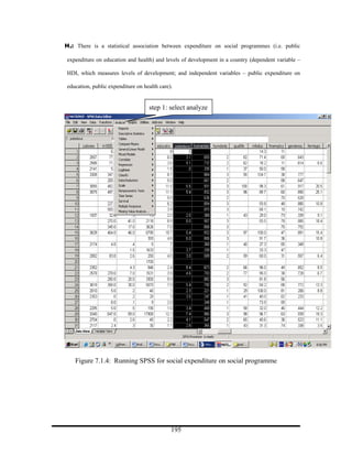
  • 28. Figure 6.1.15: Class Environment influence on Performance Figure 7.1.1: Frequency distribution of total expenditure on health as % of GDP Figure 7.1.2: Frequency distribution of total expenditure on education as % of GNP Figure 7.1.3: Frequency distribution of the Human Development Index Figure 7.1.4: Running SPSS for social expenditure on social programme Figure 7.1.5: Running bivariate correlation for social expenditure on social programme Figure 7.1.6: Running bivariate correlation for social expenditure on social programme Figure13.1.1: Categories that describe Respondents’ Position Figure13.1.2: Company’s Annual Work Volume Figure13.1.3: Company’s Labour Force – ‘on an averAge per year’ Figure13.1.4: Respondents’ main Area of Construction Work Figure13.1.5: Percentage of work ‘self-performed’ in contrast to ‘sub-contracted’ Figure13.1.6: Percentage of work ‘self-performed’ in contrast to ‘sub-contracted’ Figure 13.1.7: Years of Experience in Construction Industry Figure13.1.8: Geographical Area of Employment Figure13.1.9: Duration of service with current employer Figure13.1.10: Productivity changes over the past five years Figure 14.1.1: Characteristic of Sampled Population Figure 14.1.2: Employment Status of Respondents 28
  • 29. Listing of Tables Table 1.1.1: Synonyms for the different Levels of measurement Table 1.1.2: Appropriateness of Graphs, from different Levels of measurement Table 1.1.3: Levels of measurement1 with examples and other characteristics Table1.1.4: Levels of measurement, and measure of central tendencies and measure of variability Table1.1.5: combinations of Levels of measurement, and types of statistical Test which are application Table 1.1.6a: Statistical Tests and their Levels of Measurement Table 1.1.6b: Table 2.1.1a: Gender of Respondents Table 2.1.1b: General happiness Table 2.1.2: Social Status Table 2.1.3: Descriptive Statistics on the Age of the Respondents Table 2.1.4:“From the following list, please choose what the most important characteristic of democracy …are for you” Table 4.1.1: Respondents’ Age Table 4.1.2 (a) Univariate Analysis of the explanatory Variables Table 4.1.2(b): Univariate Analysis of explanatory Table 4.1.2 (c): Univariate Analysis of explanatory Table 4.1.3: Bivariate Relationships between academic performance and subjective Social Class (n=99) 1 29
  • 30. Table 4.1.4: Bivariate Relationships between comparative academic performance and subjective Social Class (n=108) Table 4.1.5: Bivariate Relationships between academic performance and physical exercise (n= 111) Table 4.1.6 (i): Bivariate Relationships between academic performance and instructional materials (n=113) Table 4.1.6 (ii) Relationship between academic performance and materials among students who will be writing the A’ Level Accounting Examination, 2004 Table 4.1.7: Bivariate Relationships between academic performance and Class attendance (n= 106) Table 4.1.8: Bivariate Relationship between academic performance and attendance Table 4.1.9: Bivariate Relationships between academic performance and breakfast consumption, (n=114) Table 4.1.10: Relationship between academic performances and breakfasts consumption among A’ Level Accounting students, controlling for Gender Table 4.1.11: Bivariate Relationships between academic performance and migraine (n=116) Table 4.1.12: Bivariate Relationships between academic performance and mental illnesses, (n=116) Table 4.1.13: Bivariate Relationships between academic performance and physical illnesses, (n=116) Table 4.1.14: Bivariate Relationships between academic performance and illnesses (n=116) Table 4.1.15. Bivariate Relationships between current academic performance and past performance in CXC/GCE English language Examination, (n= 112) Table 4.1.16: Bivariate Relationships between academic performance and past performance in CXC/GCE English language Examination, controlling for Gender Table 4.1.17: Bivariate Relationships between academic performance and past performance in CXC/GCE Mathematics Examination n= Table 4.1.18 (i): Bivariate Relationships between academic performance and past performance in CXC/GCE principles of accounts Examination (n= 114) 30
  • 31. Table 4.1.19 (ii): Bivariate Relationships between academic performance and past performance in CXC/GCEPOA Examination, controlling for Gender Table 4.1.20: Bivariate Relationships between academic performance and Self-Concept (n= 112) Table 4.1.21: Bivariate Relationships between academic performance and Dietary Requirements (n=116) Table 4.1.22: Summary of Tables Table 5.1.1: Frequency and percent Distributions of explanatory model Variables Table 5.1.2: Relationship between Religiosity and Marijuana Smoking (n=7,869) Table 5.1.3: Relationship between Religiosity and Marijuana Smoking controlled for Gender Table 5.1.4: Relationship between Age and marijuana smoking (n=7,948) Table 5.1.5: Relationship between marijuana smoking and Age of Respondents, controlled for sex Table 5.1.6: Relationship between academic performances and marijuana smoking, (n=7,808) Table 5.1.7: Relationship between academic performances and marijuana smoking, controlled for Gender Table 5.1.8: Summary of Tables Table 6.1.1: Age Profile of respondent Table 6.1.2: Examination Scores Table 6.1.3(a): Class Distribution by Gender Table 6.1.3(b): Class Distribution by Age Cohorts Table 6.1.3(c): Pre-Test Score by Typology of Group Table 6.1.3(c): Pre-Test Score by Typology of Group Table 6.1.4: Comparison of Examination I and Examination II Table 6.1.5: Comparison a Cross the Group by Tests 31
  • 32. Table 6.1.6: Analysis of Factors influence on Test ii Scores Table 6.1.7: Cross-Tabulation of Test ii Scores and Factors Table 6.1.8: Bivariate Relationship between student’s Factors and Test ii Scores Table 7.1.1: Descriptive Statistics - total expenditure on public health (as Percentage of GNP HRD, 1994) Table 7.1.2: Descriptive Statistics of expenditure on public education (as Percentage of GNP, Hrd, 1994) Table 7.1.3: Descriptive Statistics of Human Development (proxy for development) Table 7.1.4: Bivariate Relationships between dependent and independent Variables Table 7.1.5: Summary of Hypotheses Analysis Table8.1.1: Age Profile of Respondents (n = 16,619) Table 8.1.2: Logged Age Profile of Respondents (n = 16,619) Table 8.1.3: Household Size (all individuals) of Respondents Table 8.1.4: Union Status of the sampled Population (n=16,619) Table 8.1.5: Other Univariate Variables of the Explanatory Model Table 8.1.6: Variables in the Logistic Equation Table 8.1.7: Classification Table Table 8.1.1: Univariate Analyses Table 8.1.2: Frequency Distribution of Educational Level by Quintile Table 8.1.3: Frequency Distribution of Jamaica’s Population by Quintile and Gender Table 8.1.4: Frequency Distribution of Educational Level by Quintile Table 8.1.5: Frequency Distribution of Pop. Quintile by Household Size Table 8.1.6: Bivariate Analysis of access to Tertiary Edu. and Poverty Status Table 8.1.7: Bivariate Analysis of access to Tertiary Edu. and Geographic Locality of Residents 32
  • 33. Table 8.1.8: Bivariate Analysis of geographic locality of residents and poverty Status Table 8.1.9: Bivariate Relationship between access to tertiary level education by Gender Table 8.1.10: Bivariate Relationship between Access to Tertiary Level Education by Gender controlled for Poverty Status Table 8.1.11: Regression Model Summary Table 10.1.1: Univariate Analysis of Parental Information Table 10.1.2: Descriptive on Parental Involvement Table 10.1.3: Univariate Analysis of Teacher’s Information Table 10.1.4: Univariate Analysis of ECERS-R Profile Table 10.1.5: Bivariate Analysis of Self-reported Learning Environment and Mastery on Inventory Test Table 10.1.6: Relationship between Educational Involvement, Psychosocial and Environment involvement and Inventory Test Table 10.1.6: Relationship between Educational Involvement, Psychosocial and Environment Involvement and Inventory Test Table 10.1.8: School Type by Inventory Readiness Score Table 11.1.1: Incivility and Subjective Social Status Table 12.1.2: Have you or someone in your family known of an act of Corruption in the last 12 months? Table 12.1.3: Gender of Respondent Table 12.1.4: In what Parish do you live? Table 12.1.5: Suppose that you, or someone close to you, have been a victim of a crime. What would you do...? Table 12.1.6: What is your highest level of Education? Table 12.1.7: In terms of Work, which of these best describes your Present situation? Table 12.1.8: Which best represents your Present position in Jamaica Society? Table 12.1.9: Age on your last Birthday? Table 12.1.10: Age categorization of Respondents 33
  • 34. Table 12.1.11: Suppose that you, or someone close to you, have been a victim of a crime. what would you do... by Gender of respondent Cross Tabulation Table 12.1.12: If involved in a dispute with neighbour and repeated discussions have not made a difference, would you...? by Gender of respondent Cross Tabulation Table 12.1.13: Do you believe that corruption is a serious problem in Jamaica? by Gender of respondent Cross Tabulation Table 12.1.14: have you or someone in your family known of an act of corruption in the last 12 months? by Gender of respondent Cross Tabulation Table 14.1.1: Marital Status of Respondents Table 14.1.2: Marital Status of Respondents by Gender Table 14.1.3: Marital Status by Gender by Age cohort Table 14.1.4: Marital Status by Gender by Age Cohort Table 14.1.5 Educational Level by Gender by Age Cohorts Table 14.1.6: Income Distribution of Respondents Table 14.1.7: Parental Attitude Toward School Table 14.1.8: Parent Involving Self Table 14.1.9: School Involving Parent Table 14.1.8: Regression Model Summary Table 15.1.1: Correlations Table 15.1.2: Cross Tabulation between incivility and social status 34
  • 35. How do I obtain access to the SPSS PROGRAM? Step One: In order to access the SPSS program, the student should select ‘START’ to the bottom left hand corner of the computer monitor. This is followed by selecting ‘All programs’ (see below). Select ‘START’ and then ‘All Program 35
  • 36. Step Two: The next step to the select ‘SPSS for widows’. Having chosen ‘SPSS for widows’ to the right of that appears a dialogue box with the following options – SPSS for widows; SPSS 12.0 (or 13.0…or, 15.0); SPSS Map Geo-dictionary Manager Ink; and last with SPSS Manager. Select ‘SPSS for widows’ 36
  • 37. Step Three: Having done step two, the student will select SPSS 12.0 (or 13.0, or 14.0 or 15.0) for Widows as this is the program with which he/she will be working. Select SPSS 12.0 (or 13.0, or 14.0 or 15.0) for Widows 37
  • 38. Step Four: On selecting ‘SPSS for widows’ in step 3, the below dialogue box appears. The next step is the select ‘OK’, which result in what appears in step five. Select ‘OK’ 38
  • 40. What should I now do? The student should then select the ‘inner red box’ with the ‘X’. Select the ‘inner red box’ with the X’. 40
  • 41. Step Six: This is what the SPSS spreadsheet looks like (see Figure below). 41
  • 42. 42
  • 43. Step Seven: What is the difference here? Look to the bottom left-hand cover the spreadsheet and you will see two terms – (1) ‘Data View’ and (2) ‘Variable View’. Data View accommodates the entering of the data having established the template in the ‘Variable View’. Thus, the variable view allows for the entering of data (i.e. responses from the questionnaires) in the ‘Data View’. Ergo, the student must ensure that he/she has established the template, before any typing can be done in the ‘Data View. widow looks like ‘Data View’ Observe what the Data View 43
  • 44. 44 Variable View Observe what the ‘Variable View’ widow looks like
  • 45. CHAPTER 1 1.1.0a: INTRODUCTION This book is in response to an associate’s request for the provision of some material that would adequately provide simple illustrations of ‘How to analyze quantitative data in the Social Sciences from actual hypotheses’. He contended that all the current available textbooks, despite providing some degree of analysis on quantitative data, failed to provide actual illustrations of cases, in which hypotheses are given and a comprehensive assessment made to answer issues surrounding appropriate univariate, bivariate and/or multivariate processes of analysis. Hence, I began a quest to pursued textbooks that presently exist in ‘Research Methods in Social Sciences’, ‘Research Methods in Political Sciences’, “Introductory Statistics’, ‘Statistical Methods’, ‘Multivariate Statistics’, and ‘Course materials on Research Methods’ which revealed that a vortex existed in this regard. Hence, I have consulted a plethora of academic sources in order to formulate this text. In wanting to comprehensively fulfill my friend’s request, I have used a number of dataset that I have analyzed over the past 6 years, along with the provision of key terminologies which are applicable to understanding the various hypotheses. I am cognizant that a need exist to provide some information in ‘Simple Quantitative Data Analysis’ but this text is in keeping with the demand to make available materials for aiding the interpretation of ‘quantitative data’, and is not intended to unveil any new materials in the discipline. The rationale behind this textbook is embedded in simple reality that many undergraduate students are faced with the complex task of ‘how to choose the most appropriate statistical test’ and this becomes problematic for them as the issue of wanting to complete an 45
  • 46. assignment, and knowing that it is properly done, will plague the pupil. The answer to this question lies in the fundamental issues of - (1) the nature of the variables (continuous or discrete), and (2) what is the purpose of the analysis – is to mere description, or to provide statistical inference and/or (3) if any of the independent variables are covariates2. Nevertheless, the materials provided here are a range of research projects, which will give new information on particular topics from the hypothesis to the univariate analysis and the bivariate or multivariate analyses. 2 “If the effects of some independent variables are assessed after the effects of other independent variables are statistically removed…” (Tabachnick and Fidell 2001, 17) 46
  • 47. 1.1.0b: STEPS IN ANALYZING A HYPOTHESIS One of the challenges faced by a social researcher is how to succinctly conceptualize (i.e. define) his/her variables, which will also be operationalized (measured) for the purpose of the study. Having written a hypothesis, the researcher should identify the number of variables which are present, from which we are to identify the dependent from the independent variables. Following this he/she should recognize the level of measurement to which each variable belongs, then the which statistical test is appropriate based on the level of measurement combination of the variables. The figure below is a flow chart depicting the steps in analyzing data when given a hypothesis. The production of this text is in response to the provision of a simple book which would address the concerns of undergraduate students who must analyze a hypothesis. Among the issues raise in this book are (1) the systematic steps involved in the completion of analyzing a hypothesis, (2) definitions of a hypothesis, (3) typologies of hypothesis, (4) conceptualization of a variable, (4) types of variables, (5) levels of measurement, (6) illustration of how to perform SPSS operations on the description of different levels of measurement and inferential statistics, (7) Type I and II errors, (8) arguments on the treatment of missing variables as well as outliers, (9) how to transform selected quantitative data, (10) and other pertinent matters. The primary reason behind the use of many of the illustrations, conceptualizations and peripheral issues rest squarely on the fact the reader should grasp a thorough understanding of how the entire process is done, and the rationale for the used method. 47
  • 48. STEP ONE STEP TEN Write your Having used the Hypothesis STEP TWO test, Identify the analyze the data variables from the carefully, based on hypothesis the statistical test STEP TEN STEP THREE Choose the Define and appropriate operationalize statistical test based each variable on the combination selected from the of DV and IVS, and hypothesis STEP NINE STEP FOUR ANALYZING If statistical Inference is needed, look at the QUANTITATIVE Decide on the level combination DV and DATA of measurement IV(s) for each variable STEP EIGHT STEP FIVE If statistical association, causality Decide which or predictability is need, continue, if not variable is DV, and stop! IV STEP SIX STEP SEVEN Check for Do descriptive skewness, and/or statistics for chosen outliers in metric variables selected variables FIGURE 1.1.1: FLOW CHART: HOW TO ANALYZE QUANTITATIVE DATA? This entire text is ‘how to analyze quantitative data from hypothesis’, but based on Figure 1.1.1, it may appear that a research process begins from a hypothesis, but this is not the case. Despite that, I am emphasizing interpreting hypothesis, which is the base for this monograph starting from an actual hypothesis. Thus, before I provide you with operational definitions of 48
  • 49. variables, I will provide some contextualization of ‘what is a variable?’ then the steps will be worked out. 49
  • 50. 1.1.1a: DEFINITIONS OF A VARIABLE Undergraduates and first time researchers should be aware that quantitative data analysis are primarily based on (1) empirical literature, (2) typologies of variables within the hypothesis, (3) conceptualization and operationalization of the variables, (4) the level of measurement for each variables. It should be noted that defining a variable is simply not just the collation a group of words together, because we feel a mind to as each variable requires two critical characteristics in order that it is done properly (see Figure 1.1.2). PROPERITIES OF A VARIABLE MUTUAL EXCLUSIVITIY EXHAUSTIVNESS FIGURE 1.1.2: PROPERTIES OF A VARIABLE. In order to provide a comprehensive outlook of a variable, I will use the definitions of a various scholars so as to give a clear understanding of what it is. “Variables are empirical indicators of the concepts we are researching. Variables, as their name implies, have the ability to take on two or more values...The categories of each variable must have two requirements. They should be both exhaustive and mutually exclusive. By exhaustive, we mean that the categories of each variable must be comprehensive enough that it is possible to categorize every observation” (Babbie, Halley, and Zaino 2003, 11). “.. Exclusive refers to the fact that every observation should fit into only one category “(Babbie, Halley and Zaino 2003, 12) “A variable is therefore something which can change and can be measured.” (Boxill, Chambers and Wint 1997, 22) 50
  • 51. “The definition of a variable, then, is any attribute or characteristic of people, places, or events that takes on different values.” (Furlong, Lovelace, Lovelace 2000, 42) “A variable is a characteristic or property of an individual population unit” (McClave, Benson and Sincich 2001, 5) “Variable. A concept or its empirical measure that can take on multiple values” (Neuman 2003, 547). “Variables are, therefore, the quantification of events, people, and places in order to measure observations which are categorical (i.e. nominal and ordinal data) and non-categorical (i.e. metric) in an attempt to be informed about the observation in reality. Each variable must fill two basic conditions – (i) Exhaustiveness – the variable must be so defined that all tenets are captured as its is comprehensive enough include all the observations, and (ii) mutually exclusivity – the variable should be so defined that it applies to one event and one event only – (i.e. Every observation should fit into only one category) (Bourne 2007). One of the difficulties of social research is not the identification of a variable or variables in the study but it’s the conceptualization and oftentimes the operationalization of chosen construct. Thus, whereas the conceptualization (i.e. the definition) of the variable may (or may not) be complex, it is the ‘how do you measure such a concept (i.e. variable) which oftentimes possesses the problem for researchers. Why this must be done properly bearing in mind the attributes of a variable, it is this operational definition, which you will be testing in the study (see Typologies of Variables, below). Thus, the testing of hypothesis is embedded within variables and empiricism from which is used to guide present studies. Hypothesis testing is a technique that is frequently employed by demographers, statisticians, economists, psychologists, to name new practitioners, who are concerned about the testing of theories, and the verification of reality truths, and the modifications of social realities within particular time, space and settings. With this being said, researchers must ensure that a variable is properly defined in an effort to ensure that the stated phenomenon is so defined and measured. 51
  • 52. 1.1.1b TYPOLOGIES of VARIABLE (examples, using Figure 1.1.2, above) Health care seeking behaviour: is defined as people visiting a health practitioner or health consultant such as doctor, nurse, pharmacist or healer for care and/ or advice. Levels of education: This is denominated into the number of years of formal schooling that one has completed. Union status – It is a social arrangement between or among individuals. This arrangement may include ‘conjugal’ or a social state for an individual. Gender: A sociological state of being male or female. Per capita income: This is used a proxy for income of the individual by analyzing the consumption pattern. Ownership of Health insurance: Individuals who possess of an insurance polic/y (ies). Injuries: A state of being physically hurt. The examples here are incidences of disability, impairments, chronic or acute cuts and bruises. Illness: A state of unwellness. Age: The number of years lived up to the last birthday. Household size - The numbers of individuals, who share at least one common meal, use common sanitary convenience and live within the same dwelling. Now that the premise has been formed, in regard to the definition of a variable, the next step in the process is the category in which all the variables belong. Thus, the researcher needs to know the level of measurement for each variable - nominal; ordinal; interval, or ration (see 1.1.2a). 52
  • 53. 1.1.2a: LEVELS OF MEASUREMENT3: Examples and definitions Nominal - The naming of events, peoples, institutions, and places, which are coded numerical by the researcher because the variable has no normal numerical attributes. This variable may be either (i) dichotomous, or (ii) non-dichotomous. Dichotomous variable – The categorization of a variable, which has only two sub- groupings - for example, gender – male and female; capital punishment – permissive and restrictive; religious involvement – involved and not involved. Non-dichotomous variable – The naming of events which span more than two sub-categories (example Counties in Jamaica – Cornwall, Middlesex and Surrey; Party Identification – Democrat, Independent, Republican; Ethnicity – Caucasian, Blacks, Chinese, Indians; Departments in the Faculty of Social Sciences – Management Studies, Economics, Sociology, Psychology and Social Work, Government; Political Parties in Jamaica – Peoples’ National Party (PNP), Jamaica Labour Party (JLP), and the National Democratic Movement (NDM); Universities in Jamaica – University of the West Indies; University of Technology, Jamaica; Northern Caribbean University; University College of the Caribbean; et cetera) Ordinal - Rank-categorical variables: Variables which name categories, which by their very nature indicates a position, or arrange the attributes in some rank ordering (The examples here are as follows i) Level of Educational Institutions – Primary/Preparatory, All-Age, Secondary/High, Tertiary; ii) Attitude toward gun control – strongly oppose, oppose, favour, strongly favour; iii) Social status – upper--upper, upper-middle, middle-middle, lower-middle, lower class; iv) Academic achievement – A, B, C, D, F. Interval or ratio These variables share all the characteristics of a nominal and an ordinal variable along with an equal distance between each category and a ‘true’ zero value – (for example – age; weight; height; temperature; fertility; votes in an election, mortality; population; population growth; migration rates, . Now that the definitions and illustrations have been provided for the levels of measurement, the student should understand the position of these measures (see 1.1.2b). 3 Stanley S. Stevens is created for the development of the typologies of scales – level of measurement – (i) nominal, (ii) ordinal, (iii) interval and (iv) ratio. (see Steven 1946, 1948, 1968; Downie and Heath 1970) 53
  • 54. Dichotomy (or Dichotomous variable Typologies of Gender Science Book Non- Fictional Male Female Pure Applied Fictional Alive Dead Induction Deduction Non- Parametric Burial Non-burial parametric statistics statistics Religious Non-religious Non- use primary use secondary Decomposed data data service service decomposed Figure 1.1.3: Illustration of dichotomous variables 54
  • 55. 1.1.2b: RANKING LEVELS OF MEASUREMENT RATIO highes t INTERVAL ORDINAL lowest NOMINAL Figure 1.1.4: Ranking of the levels of measurement The very nature of levels of measurement allows for (or do not allow for) data manipulation. If the level of measurement is nominal (for example fiction and non-fiction books), then the researcher does not have a choice in the reconstruction of this variable to a level which is below it. If the level of measurement, however, is ordinal (for example no formal education, primary, secondary and tertiary), then one may decide to use a lower level of measure (for example below secondary and above secondary). The same is possible with an interval variable. The social scientist may want to use one level down, ordinal, or two levels down, nominal. This is equally the same of a ratio variable. Thus, the further ones go up the pyramid, the more scope exists in data transformation. 55
  • 56. Table 1.1.1: Synonyms for the different Levels of measurement Levels of Measurement Other terms Nominal Categorical; qualitative, discrete4 Ordinal Qualitative, discrete; rank-ordered; categorical Interval/Ratio Numerical, continuous5, quantitative; scale; metric, cardinal Table 1.1.2: Appropriateness of Graphs for different levels of measurement Levels of Measurement Graphs Bar chart Pie chart Histogram Line Graph Nominal √ √ __ __ √ √ __ __ Ordinal __ __ √ √ Interval/Ratio (or metric) 4 Discrete variable – take on a finite and usually small number of values, and there is no smooth transition from one value or category to the next – gender, social class, types of community, undergraduate courses 5 Continuous variables are measured on a scale that changes values smoothly rather than in steps 56
  • 57. Table 1.1.3: Levels of measurement6 with Examples and Other Characteristics Levels of Measurement Nominal Ordinal Interval Ratio Examples Gender Social class Temperature Age Religion Preference Shoe size Height Political Parties Level of education Life span Weight Race/Ethnicity Gender equity Reaction time Political Ideologies levels of fatigue Income; Score on an Exam. Noise level Fertility; Population of a country Job satisfaction Population growth; crime rates Mathematical properties Identity Identity Identity Identity ____ Magnitude Magnitude Magnitude ____ _____ Equal Interval Equal interval ____ _____ _____ True zero Mathematical Operation(s) None Ranking Addition; Addition; Subtraction Subtraction; Division; Multiplication Compiled: Paul A. Bourne, 2007; a modification of Furlong, Lovelace and Lovelace 2000, 74 6 “Levels of measurement concern the essential nature of a variable, and it is important to know this because it determines what one can do with a variable (Burham, Gilland, Grant and Layton-Henry 2004, 114) 57
  • 58. Table1.1.4: Levels of measurement, Measure of Central Tendency and Measure of Variability Levels of Measurement Measure of central tendencies Measure of variability Mean Mode Median Mean deviation Standard deviation Nominal NA √ NA NA NA Ordinal NA √ √ NA NA Interval/Ratio7 √ √ √ √ √ NA denotes Not Applicable 7 Ratio variable is the highest level of measurement, with nominal being first (i.e. lowest); ordinal, second; and interval, third. 58
  • 59. Table1.1.5: Combinations of Levels of measurement, and types of Statistical test which are applicable8 Levels of Measurement Statistical Test Dependent Independent Variable Nominal Nominal Chi-square Nominal Ordinal Chi-square; Mann-Whitney Nominal Interval/ratio Binomial distribution; ANOVA; Logistic Regression; Kruskal-Wallis Discriminant Analysis Ordinal Nominal Chi-square Ordinal Ordinal Chi-square; Spearman rho; Ordinal Interval/ratio Kruskal-Wallis H; ANOVA Interval/ratio Nominal ANOVA; Interval/ratio Ordinal Interval/ratio Interval/ratio Pearson r, Multiple Regression Independent-sample t test Table 1.1.5 depicts how a dependent variable, which for example is nominal, which when combined with an independent variable, Nominal, uses a particular statistical test. 8 One of the fundamental issues within analyzing quantitative data is not merely to combine then interpret data, but it is to use each variable appropriately. This is further explained below. 59
  • 61. STATISTICAL TESTS AND THEIR LEVELS OF MEASUREMENT Test Independent Dependent Variable variable Chi-Square (χ2) Nominal, Ordinal Nominal, Ordinal Mann-Whitney U Dichotomous Nominal, Ordinal test Kruskal-Wallis H Non-dichotomous, Ordinal, or skewed9 test Ordinal Metric Pearson’s r Normally distributed10 Normally distributed Metric Metric Linear Regress Normally distributed Normally distributed Metric, dummy Metric Independent Dichotomous Normally distributed Samples Metric T-test AVONA Nominal, Ordinal Normally distributed (non-dichotomous11) Metric Logistic regression Metric, dummy Dichotomous (skewed values or otherwise Discriminant Metric, dummy Dichotomous (normally distributed analysis value) Notes to Table 1.1.6b Chi-Square (χ2) Used to test for associations between two variables Mann-Whitney U test Used to determine differences between two groups Kruskal-Wallis H test Used to determine differences between three or more groups Pearson’s r Used to determine strength and direction of a relationship between two values Linear Regression Used to determine strength and direction of a relationship between two or more values Independent Samples T-test Used to determine difference between two groups AVONA Used to determine difference between three or more groups Logistic regression Used to predict relationship between many values Discriminant analysis Used to predict relationship between many values 9 Skewness indicates that there is a ‘pileup’ of cases to the left or right tail of the distribution 10 Normality is observed, whenever, the values of skewness and kurtosis are zero 11 Non-dichotomous (i.e. polytomous) which denotes having many (i.e. several) categories 61
  • 62. LEVELS OF MEASURMENT AND THEIR MEASURING ASSOCIATION LEVELS OF MEASUREMENT NOMINAL ORDINAL INTERVAL/RATIO Lambda Gamma Pearson’s r Cramer’s V Somer’s D Contingency coefficients Kendall ‘s tau-B Phi Kendall’s tau-c Figure 1.1.5: Levels of measurement ‫ג‬ Lambda ( ) – This is a measure of statistical relationship between the uses of two nominal variables Phi (Φ) – This is a measure of association between the use of two dichotomous variables (i.e. dichotomous dependent and dichotomous independent) – [Φ = √[ χ2/N] Cramer’s V (V) – This is a measure of association between the use of two nominal variables (i.e. in the event that there is dichotomous dependent and dichotomous independent) – V = √[ χ2/N(k – 1)] is identical to phi. γ Gamma ( ) – This is used to measure the statistical association between ordinal by ordinal variable Contingency coefficient (cc) – Is used for association in which the matrix is more than 2 X 2 (i.e. 2 for dependent and 2 for the independent – for example 2X3; 3X2; 3X3 …) - √ [χ2/ χ2 + N] Pearson’s r – This is used for non-skewed metric variables - n∑xy - ∑x.∑y √ [n∑x2 – (∑x) 2 - [n∑y2 – (∑y) 2 62
  • 63. 1.1.3: CONCEPTUALIZING DESCRIPTIVE AND INFERENTIAL STATISTICS Research is not done in isolation from the reality of the wider society. Thus, the social researcher needs to understand whether his/her study is descriptive and/or inferential as it guides the selection of certain statistical tools. Furthermore, an understanding of two constructs dictate the extent to which the analyst will employ as there is a clear demarcation between descriptive and inferential statistics. In order to grasp this distinction, I will provide a number of authors’ perspectives on each terminology. “Descriptive statistics describe samples of subjects in terms of variables or combination of variables” (Tabachnick and Fidell 2001, 7) “Numerical descriptive measures are commonly used to convey a mental image of pictures, objects, tables and other phenomenon. The two most common numerical descriptive measures are: measures of central tendencies and measures of variability (McDaniel 1999, 29; see also Watson, Billingsley, Croft and Huntsberger 1993, 71) “Techniques such as graphs, charts, frequency distributions, and averages may be used for description and these have much practical use” (Yamane 2973, 2; see also Blaikie 2003, 29; Crawshaw and Chambers 1994, Chapter 1) “Descriptive statistics – statistics which help in organizing and describing data, including showing relationships between variables” (Boxill, Chamber and Wind 1997, 149) 63
  • 64. “We’ll see that there are two areas of statistics: descriptive statistics, which focuses on developing graphical and numeral summaries that describes some…phenomenon, and inferential statistics, which uses these numeral summaries to assist in making… decisions” (McClave, Benson, Sinchich 2001, 1) “Descriptive statistics utilizes numerical and graphical methods to look for patterns in a data set, to summarize the information revealed in a data set, and to present the information in a convenient form” (McClave, Benson and Sincich 2001, 2) “Inferential statistics utilizes sample data to make estimates, decisions, predictions, or other generalizations about a larger set of data” (McClave, Benson and Sincich 2001, 2) “The phrase statistical inference will appear often in this book. By this we mean, we want to “infer” or learn something about the real world by analyzing a sample of data. The ways in which statistical inference are carried out include: estimating…parameters; predicting…outcomes, and testing…hypothesis …” (Hill, Griffiths and Judge 2001, 9). Inferential statistics is not only about ‘causal’ relationships; King, Keohane and Verba argue that it is categorized into two broad areas: (1) descriptive, and (2) causal inference. Thus, descriptive inference speaks to the description of a population from what is made possible, the sample size. According to Burham, Gilland, Grant and Layton-Henry (2004) state that: Causal inferences differ from descriptive ones in one very significant way: they take a ‘leap’ not only in terms of description, but in terms of some specific causal 64
  • 65. process [i.e. predictability of the variables]” (Burham, Gilland, Grand and Layton- Henry 2004, 148). In order that this textbook can be helping and simple, I will provide operational definitions of concepts as well as illustration of particular terminologies along with appropriateness of statistical techniques based on the typologies of variable and the level of measurement (see in Tables 1.1.1 – 1.1.6, below). 65
  • 66. CHAPTER 2 2.1.0: DESCRIPTIVE STATISTICS The interpretation of quantitative data commences with an overview (i.e. background information on survey or study – this is normally demographic information) of the general dataset in an attempt to provide a contextual setting of the research (descriptive statistics, see above), upon which any association may be established (inferential statistics, see above). Hence, this chapter provides the reader with the analysis of univariate data (descriptive statistics), with appropriate illustration of how various levels of measurement may be interpreted, and/or diagrams chosen based on their suitability. A variable may be non-metric (i.e. nominal or ordinal) or metric (i.e. scale, interval/ratio). It is based on this premise that particular descriptive statistics are provide. In keeping with this background, I will begin this process with non-metric, then metric data. The first part of this chapter will provide a thorough outline of how nominal and/or ordinal variables are analyzed. Then, the second aspect will analyze metric variables. 66
  • 67. STEP ONE Ensure that the STEP TEN variable is non- Analyze the output metric (e.g. Gender, STEP TWO (use Table 2.1.1a) general happiness) Select Analyze STEP TEN STEP THREE Select descriptive select paste or ok statistics HOW TO DO DESCRIPTIVE STEP NINE STATISTICS FOR A STEP FOUR NO-METRIC Choose bar or pie graphs VARIABLE? select frequency STEP FIVE STEP EIGHT select the non-metric select Chart variable STEP SEVEN STEP SIX select mode or mode and median (based on if the select statistics at the variable is nominal or end ordinal respective Figure 2.1.0: Steps in Analyzing Non-metric data 67
  • 68. 2.1.1a: INTERPRETING NON-METRIC (or Categorical) DATA NOMINAL VARIABLE (when there are not missing cases) Table 2.1.1a: Gender of respondents Frequency Percent Valid Percent Male 150 69.4 69.4 Gender: Female 66 30.6 30.6 Total 216 100.0 100.0 Identifying Non-missing Cases: When there are no differences between the percent column and those of the valid percent column, then there are no missing cases. How is the table analyzed? Of the sampled population (n=21612), 69.4% were males compared to 30.6% females. 12 The total number of persons interviewed for the study. It is advisable that valid percents are used in descriptive statistics as there may be some instances then missing cases are present with the dataset, which makes the percent figure different from those of the valid percent (Table 2.1.1b). 68
  • 69. NOMINAL VARIABLE: Establishment of when missing cases Table 2.1.1b: General Happiness Frequency Percent Valid Percent Very happy 467 30.8 31.1 General Happiness: Pretty happy 872 57.5 58.0 Not too happy 165 10.9 11.0 Missing Cases 13 0.9 - Total 1,517 100.0 100.0 Identifying Missing Cases: In seeking to ascertain missing data (which indicates that some of the respondents did no answer the specified question), there is a disparity between the values for percent and those in valid percent. In this case, 13 of 1,517 respondents did not answer question on ‘general happiness’. In cases where there is a difference between the two aforementioned categories (i.e. percent and valid percent), the student should remember to use the valid percent. The rationale behind the use of the valid percent is simple, the research is about those persons who have answered and they are captured in the valid percent column. Hence, it is recommended that the student use the valid percent column at all time in analyzing quantitative data. Interpretation: Of the sampled population (n=1,517), the response rate is 99.1% (n=1,504)13. Of the valid responses (n=1,504), 31.1% (n=467) indicated that they were ‘very happy’, with 58.0% (n=872) reported being ‘pretty happy’, compared to 11.0% (n=165) who said ‘not too happy’. 13 Because missing cases are within the dataset (13 or 0.9%), there is a difference between percent and valid percent. Thus, care should be taken when analyzing data. This is overcome when the valid percents are used. 69
  • 70. Owing to the typology of the variable (i.e. nominal), this may be presented graphical by either a pie graph or a bar graph. Pie graph Female, 30.6, 31% Male, 69.4, 69% Figure 2.1.1: Respondents’ gender OR Bar graph 70 60 50 40 30 20 10 0 Male Female Figure 2.1.2: Respondents’ gender 70
  • 71. ORDINAL VARIABLE Table 2.1.2: Subjective (or self-reported) Social Class Frequency Percent Valid Percent Social class: Lower 100 46.3 46.3 Middle 104 48.1 48.1 Upper 12 5.6 50.6 Total 216 100.0 100.0 Interpreting the Data in Table 2.1.2: When the respondents were asked to select what best describe their social standing, of the sampled population (n=216), 46.3% reported lower (working) class, 48.1% revealed middle class compared to 5.6% who said upper middle class. Based on the typology of variable (i.e. ordinal), the graphical options are (i) pie graph and/or (2) bar graph. Note: In cases where there is no difference between the percent column and that of valid percent, researchers infrequently use both columns. The column which is normally used is valid percent as this provides the information of those persons who have actually responded to the specified question. Instead of using ‘valid percent’ the choice term is ‘percent’. 71
  • 72. 50 45 48.1 40 46.3 35 30 25 20 15 10 5 5.6 0 Lower class Middle class Upper middle class Figure 2.1.3: Social class of respondents Or Upper middle class, 5.6 Lower class, 46.3 Middle class, 48.1 Figure 2.1.4: Social class of respondents 72
  • 73. 2.1.1b: STEPS IN INTERPRETING METRIC VARIABLE: METRIC (i.e. scale or interval/ratio) STEP ONE STEP TEN Know the metric variable (Age) STEP TWO Analyze the output (use Table 2.1.3) Select Analyze STEP TEN STEP THREE Select descriptive select paste or ok statistics HOW TO DO STEP NINE DESCRIPTIVE STATISTICS FOR STEP FOUR Choose histogram A METRIC with normal curve VARIABLE? select frequency STEP FIVE STEP EIGHT select Chart select the metric variable STEP SIX STEP SEVEN select mean, select statistics at standard deviation, the end skewness Figure 2.1.5: Steps in Analyzing Metric data 73
  • 74. INTERPRETING METRIC DATA: METRIC (i.e. scale or interval/ratio) VARIABLE Table 2.1.3: Descriptive statistics on the Age of the Respondents N Valid 216 Missing 0 Mean 20.33 Median 20.00 Mode 20 Std. Deviation 1.692 Skewness 2.868 Std. Error of Skewness .166 Of the sampled population (n=216), the mean age of the sample was 20 yrs and 4 months (i.e. 4 = 0.33 x 12) ± 1 yr. and 8 months (i.e. 8 = 0.692 x 12), with a skewness of 2.868 yrs. Statistically an acceptable skewness must be less than or equal to 1.0. Hence, this skewness in this sample is unacceptable, as it is an indicator of errors in the reporting of the data by the respondents. With this being the case, the researcher (i.e. statistician) has three options available at his/her disposal. They are (1) to remove the skewness, (2) not use the data – because of the high degree of errors and (3) use the median instead of the mean. It should be noted that all the measure of central tendencies (i.e. the arithmetic mean, arithmetic mode and the arithmetic median) are about the same (i.e. mean – 20.33, mode – 20.0, and median – 20.0). This situation is caused by extreme values in the data set. Hence, in this case, the arithmetic mean is disported by the values (or value) and so it is not advisable this be used to indicate the centre of the distribution. (See below how this is done in SPSS) The figure below is to enable readers to have a systematic plan of ‘how to arrive at the SPSS output’ for analyzing a metric variable (for example age of respondents). Following the figure, I implement the plan in an actual SPSS illustration of how this is done. 74
  • 75. Step One: ANALYZE Figure 2.1.6: ‘Running’ SPSS for a Metric variable 75
  • 76. Step Two: Descriptive statistics Figure 2.1.7: ‘Running’ SPSS for a Metric variable 76
  • 77. Step Three: select Frequency Figure 2.1.8: ‘Running’ SPSS for a Metric variable 77
  • 78. Step Four: Select the metric variable – The metric variable – in this case is age Figure 2.1.9: ‘Running’ SPSS for a Metric variable 78
  • 79. Step Five select the metric variable from over here to to here Figure 2.1.10: ‘Running’ SPSS for a Metric variable 79
  • 80. to the end of Step Five, you’ll see statistics select it Figure 2.1.11: ‘Running’ SPSS for a Metric variable 80
  • 81. Step Six: A metric variable requires that you do the me an Choose the following: SD, minimum, range select skewness, kurtosis Figure 2.1.12: ‘Running’ SPSS for a Metric variable 81
  • 82. Step Seven: To the end of Step Five, you will see Charts; this means you should select Histogram with normal curve Figure 2.1.13: ‘Running’ SPSS for a Metric variable 82
  • 83. Step Nine: select ‘run’, which is this Key Step Eight: Highlight the argument Figure 2.1.14: ‘Running’ SPSS for a Metric variable 83
  • 84. Step Ten: Final Output, which the researcher will now analyze Figure 2.1.15: ‘Running’ SPSS for a Metric variable 84
  • 85. Histogram 120 Step Eleven: 100 This is pictorial of the distribution of the metric variable, age 80 60 n u q F y c e r 40 20 Mean = 34.95 Std. Dev. = 13.566 0 N = 1,280 20 40 60 80 Age on your last birthday? Figure 2.1.16: ‘Running’ SPSS for a Metric variable 85
  • 86. 2.1.2a: MISSING (i.e. NON-RESPONSE) CASES Table 2.1.4: “From the following list, please choose what the most important characteristic of democracy …are for you” Frequency Percent Open and fair election 314 23.5 An economic system that guarantees a dignified salary 177 13.2 Freedom of speech 321 24.0 Equal treatment for everybody 295 22.0 Respect for minority 35 2.6 Majority rules 54 4.0 Parliamentarians who represented their electorates 52 3.9 A competitive party system 47 3.5 Don’t know/No answer 43 3.214 Total 1338 100.0 Source: Powell, Bourne and Waller 2007, 11 Of the sampled population (n=1,338), when asked “From the following list, please choose what is four you the most important characteristic of democracy …?”, 23.5% (n=314) ‘open and fair elections’ 13.2% (n=177) remarked ‘An economic system that guarantees a dignified salary’, 24.0% (n=321) said ’Freedom of speech’ , 22.0% (n=295) indicated ‘Equal treatment for everybody by courts of law’, 2.6% (n=35) mentioned ‘Respect for minorities’, 4.0% (n=54) felt ‘Majority rule’, 3.9% (n=52) believed ‘Members of Parliament who represent their electors’, and 3.5% (n=47) informed that ‘A competitive party system’ compared to 3.2% (n=43) who had no answer – (i.e. ‘Don’t know/No answer), which is referred to as ‘missing values’ or, see note 4. 14 “Don’t know/no answer” is an issue of fundamental importance in survey research. This is called non- response. 86
  • 87. The issue of non-response becomes problematic whenever it is approximately 5%, or more (see for example George and Mallery 2003, chapter 4; Tabachnick and Fidell 2001, chapter 4; Thirkettle 1988, 10). Missing data are simply not just about ‘non-response’, but they may distort the interpretation of data in case of ‘inferential statistics’. In some instances that they are so influential that they create what is called, Type II error. According to Thirkettle 1998, “Unless every person to be interviewed is interviewed the results will not be valid. Non-response must therefore be kept to negligible proportions” (Thirkettle 1988, 10). Thirkettle’s perspective is idealistic, and this is not supported by ant of the other scholars to which I have read (see for example Babbie, Halley and Zaino 2003; George and Mallery 2003; Tabachnick and Fidell 2001; Bobko 2001; Willemsen 1974). The issue of what is an unacceptable ‘non-response rate’ is 20%. When this marker is reached or surpassed, researchers are inclined not to use the variable. Thus, in the case of Table 2.1.4, a non-response rate of 3.2% is considered to be negligible. Furthermore, missing data is simply not about ‘non-response’ from the interviewed but it is the difficulty of generalizability that it may cause, which posses the problem in data analysis. “Its seriousness depends on the pattern of missing data, how much is missing, and why it is missing” (Tabachnick and Fidell 2001, 58). According to Tabachnick and Fidell (2001): The pattern of missing data is more important than the amount missing. Missing values scattered randomly through a data matrix pose less serious problems. Nonrandomly missing values, on the other hand, are serious no matter how few of them there are because they affect the generalizability of results (Tabachnick and Fidell 2001, 58). He continues that If only a few data points, say, 5% or less, are missing in a randomly pattern form a large data set, the problems are less serious and almost any procedure for handling missing vales yields similar results (Tabachnick and Fidell 2001, 59). 87
  • 88. 2.1.2b: TREATING MISSING (i.e. NON-RESPONSES) CASES Unlike a dominant theory which is generally acceptable by many scholars, the construct of missing data is fluid. Thus, I will be forwarding some of the arguments that exist on the matter. Fundamentally, the handling of missing cases primarily rest in the following categorizations. These are – (1) if the cases are less than 5%, (2) number of non-response exceeds 20% and (3) randomly or non-randomly distributed with the dataset. Scholars, such as Thirkettle (1988) ands Tabachnick and Fidell (2003) believe that in the event that the number of such cases are less than or equal to 5%, they are acceptable. On the other hand, in the event when such non-responses are more than or equal to 20%, those variables are totally dropped from the data analysis. Thus, according to Tabachnick and Fidell 2001, chapter 4; George and Mallery 2003, chapter 4, these are the available options in manipulating missing cases: • drop all cases with them; • deletion of cases (i.e. this is a default function of SPSS, SAS, and SYSTAT); • impute values for those missing cases-  insert series mean15,16 mean of nearby points, median of nearby points;  using regression – (i) linear trends at point, and (ii) linear interpolation;  expectation maximization (EM)17, 18  using prior knowledge, and  multiple imputation 15 “It is best to avoid mean substitution unless the proportion of missing is very small and there are no other options available to you” (Tabachnick and Fidell 2001, 66) 16 “Series mean is by far the most frequently used method” (George and Mallery 2003, 50) 17 “EM methods offer the simplest and most reasonable approach to imputation of missing data. as long as you have access to SPSS MVA …(Tabachnick and Fidell 2001, 66) 18 “Regression or EM. These methods are the most sophisticated and are generally recommended” (de Vaus 2002, 69) 88
  • 89. CONCLUSION The issue of how to ‘treat missing variables’ is as unresolved as the inconclusiveness of a ‘Supreme Being, God’ and as the divergence of views on the same. One scholar forwards the view that 10% of the data cases can be missing for them to be replaced by ‘mean values’ (Marsh 1988), whereas another group of statisticians Tabachnick and Fidell (2004) believed that not more than 5% of the cases should be absence, for replacement by any approach. The latter scholars, however, do not think that a 5% benchmark in and of itself is an automatic valuation for replacement but that the researcher should test this by way of cross tabulation. This is done with some other variable(s) in an attempt to ascertain if any difference exists between the responses and the non-responses. If on concluding that no-difference is present between the responses and the non-responses, it is only then that they subscribe to replacement of missing data within the dataset. Hence, missing data are replaced by one of the appropriate mathematical technique – ‘series mean’, ‘mean of nearby points’, ‘median of nearby points’, ‘linear interpolation’, and/or ‘linear trends at points’. The perspective is not the dominant viewpoint as within the various disciplines, some scholars are ‘purist’ and so take a fundamental different stance from other who may relax this somewhat. One of the difficulties is for social researchers and upcoming practitioners of the craft are to grasp – their discipline’s delimitations and some of the rationale which are present therein in an effort to concretize their own position grounded by some empiricism. In keeping with this tradition, I will present a discourse on the matter; and I 89
  • 90. will add that scholars should be mindful of what obtains within their craft. It should be noted that sometimes these premises are ‘best practices’ and in other instances, they are merely guide and not ‘laws’. On the other hand, in a dialogue with Professor of Demography at the University of the West Indies, Mona, C. Uche, PhD., he being a ‘purist’ of the Chicago School, believe than the arbitrary substitution of non-responses can be a misrepresentation of the views of the non-respondents, and so he advice researcher do to take that route, even if the cases are less than 5%. In a monologue with Professor of Applied Sociology, Patricia Anderson, PhD., from the same Chicago School held the view that while it is likely to replace missing data point for a variable, in the case in Jamaica non-response should be taken as is. She argued that no answer, in Jamaica, is somewhat different from those who are indicated choiced responses. Thus, if the researcher substitution ‘missing cases’ with mean value or any other technique for that rather, he/she runs the risk of misrepresenting the social reality. With Marsh, Tabachnick and Fidell, Uche, and Anderson, we may conclude this discourse has many more time left in its wake. Thus, the ‘treatment of missing values’ must be left up to the researcher within the context of society and any validation of a chosen perspective. 90
  • 91. CHAPTER 3 3.1.0: HYPOTHESIS: INTRODUCTION All research is based on the premise of an investigation of some unknown phenomenon. Quantitative studies, on the other hand, are not merely to provide information but it is substantially hinged on the foundation of hypothesis testing, as this allows for some logical way of thinking. Therefore, this chapter focuses on the continuation of Chapter 2, while further the research process, which is the use of hypothesis, and the use of appropriate statistical test in an effort to validate the hypothesis of the research, in question. One author argues that it is widely accepted that studies should be geared towards testing hypothesis (Blaikie 2003, 13). He continues that “when research starts out with one or more hypotheses, they should ideally be derived from a theory of some kind, preferably expressed in for of a set of propositions” (Blaikie 2003, 14). The use of hypothesis, in objectivism, is not limited to examination of some past theories, but without this the realities that social scientists seek to explore become more so a maze, with no ending in sight. According to Blaikie 2003, “Hypotheses that are plucked out of thin air, or are just based on hunches, usually makes limited contributions to the development of knowledge because they are unlikely to connect with the existing state of knowledge (Blaikie 2003, 14). Thus, I will begin the definition of the construct, hypothesis. Then I will proceed with a full interpretation of the results beginning with the germane univariate data (see 91
  • 92. for example chapter 2) followed by the most suitable associational test (see chapter 1), given the levels of measurement. 3.1.1: DEFINITIONS OF HYPOTHESIS “A hypothesis is a preposition of a relationship between two variables: a dependent and an independent” (Babbie, Hally, and Zaino 2003, 12). The dependent variable is influenced by external stimuli (or the independent variable), and the independent variable is actually acting on its own to “cause”, or “lead to” an impact on the dependent. According to Babbie, Hally and Zaino, “A dependent variable is the variable you are trying to explain (Babbie, Hally and Zaino 2003, 13). Boxill, Chambers and Wint (1997), on the other hand, write that a “Hypothesis – a non- obvious statement which makes an assertion establishing a testable base about a doubtful or unknown statement (Boxill, Chambers and Wint 1997, 150). With Neuman (2003) stating that a hypothesis is “The statement from a causal explanation or proposition that has a least one independent and one dependent variable, but it has yet to be empirically tested” (Neuman 2003, 536). Another group of scholars write that a hypothesis is “A statement about the (potential) relationship between the variables a researcher is studying. They are usually testable statements in the form of predictions about relationships between the variables, and are used to guide the design of studies.” (Furlong, Lovelace and Lovelace 2000, G8). Every hypothesis must have two attributes. These are (1) a dependent variable, and (2) an independent variable. Thus, embedded within each hypothesis are at least two variables. So as to make this easily understandable, I will a few examples. • There is an association between breakfast consumption and ones academic performance – DV (dependent variable) – academic performance; and IV (independent variable) – breakfast consumption. • Determinants of wellbeing of the Jamaica elderly (such a hypothesis require the use of multiple regression analysis as they possesses a number 92
  • 93. of different causal factors. Hence, the DV is wellbeing. And IVs are – educational attainment; biomedical conditions; age cohorts of the elderly (young elderly, old-elderly and the oldest-old elderly); union status; area of residence; social support; employment status; number of people in household; financial support; environment conditions; income; cost of health care; exercise; 3.1.2: TYPOLOGIES OF HYPOTHESIS In social research hypotheses are categorized as either (1) theoretical or (2) statistical. According to Blaikie (2003) “Statistical hypotheses deal only with the specific problem of estimating whether a relationship found in a probability sample also exists in the population” (Blaikie 2003, 178). This textbook will only use statistical hypotheses. Furthermore, statistical hypotheses are written as null, Ho19 and alternative, Ha20. The Ho indicates no statistical association in the population; whereas the Ha denotes a statistical association in the population between the dependent and the independent variable (s). Furthermore, a statistical hypothesis may be either directional or non-directional. 19 In regression analysis, the null hypothesis, Ho: β = 0. 20 When using regression analytic technique, the alternative hypothesis, Ha : β ≠ 0 93
  • 94. 3.1.3: DIRECTIONAL AND NON-DIRECTIONAL HYPOTHESES NON-DIRECTIONAL HYPOTHESES Non-directional hypotheses exist whenever the researcher has not specified any direction for the hypothesis: The examples here are as follows:  Politicians are more corrupt than Clergymen;  There is an association between number of hours spent studying and the examination results had;  Men are less likely to be personal secretaries than women;  curative care, preventative care, social class, educational attainment, and types of school attended are determinants of well-being DIRECTIONAL HYPOTHESES Directional hypotheses exist when the researcher specifies a direction for the hypothesis: 1. Positive relationship – meaning an increase in one variable sees an increase in other variable(s): -  An increase in ones age is associated with a direct change in more years of worked experiences;  There is a positive relationship between educational attainment and income received;  There is a direct relationship between fertility and population increases. 2. Negative relationship – meaning an increase in one variable result in a reduction in other variable(s): - 94
  • 95. An increase in ones age is associated with a reduction in physical functioning;  There is an inverse relationship between educational attainment and the fertility of a woman;  There is an inverse relationship between the number of hours the West Indian crickets spent practice and them failing; 3.1.4a: OUTLIERS Despite the fact that it is mathematically appropriate to compute the mean for interval and ratio data [i.e. metric or scale data], there are times when the median may be more descriptive measure of central tendency for interval and ratio data because highly irregular values (called outliers) [exist] in the data set [and these] may affect the value of the mean (especially in small sets of scores), but they have no effect on the value of the median” (Furlong, Lovelace and Lovelace 2000, 94-95). It is on this premise that median is used instead of the mean as a measure of central tendency. Statistically, the mean is affect by extremely large or small values, which explains the reason for the skewness that exists in the descriptive statistics for interval/ratio variables. Thus, care must be taken in using highly skewed data for a hypothesis. In the event that the researcher intends to use the skewed variable as is, he/she should ensure that the statistical test is appropriate for this situation (see Chapter I). Otherwise, the information that is garnered is of no use. 95
  • 96. In the event that outliers are detected within a variable, the researcher should explore his/her available options before a decision is taken on any particular event. If skewness (i.e. an indicator of outliers) is detected, this does not presuppose that mean is inappropriate as some statisticians argue that an acceptable value is approximately ± 1. The social research should be cognizant that outliers are not only an issue in metric variable but may also be present in categorical variables. According to Tabachnick and Fidell: Rummel (1970) suggests deleting dichotomous variables with 90-10 splits between categories or more both because the correlation coefficients between these variables and others are truncated and because the scores for the cases in the small category are more influential than those in the category with numerous cases (Tabachnick and Fidell 2001, 67) 3.1.4b: REASONS for OUTLIERS  data recording entry;  Instrumentation error - the item entered in the particular category, may be different from those previously entered. 3.1.4c: IDENTIFICATION of OUTLIERS  mathematically – using skewness;  graphical approach. 3.1.4d: TREATMENT of OUTLIERS  If data entry – correct this by using the questionnaire, then redo the analysis;  If instrumentation – drop the case(s). 96
  • 97. 3.1.5: STATISTICAL APPROACHES FOR ADDRESSING SKEWNESS However, if the skewness happens to be more than the absolute value of 1 (i.e. the numerical value without taking into consideration the sign for the value), the following should be sought in an attempt to either (i) remove the skewness, or (ii) reduce the skewness. These options are as follows: i) Log10 the value; ii) Loge or ln, the value; iii) Square root, the variable; iv) Square, the variable. In the event that we are unable to reduce or remove skewness, the researcher should not use the mean as a measure of the ‘average’ as it is affect by outliers21 which are present within the dataset. In addition, he/she should ensure that the variable in question, for the purpose of hypothesis testing, is in keeping with a statistical test that is able to accommodate such a skewness (see Chapter I). In order to provide a better understanding the construct in this text, I will present each hypothesis in a new chapter. 21 “An outlier is a case with such an extreme value on one variable ( a univariate outlier) or such a strange combination of scores on two or more variables (multivariate outlier) that they distort statistics (Tabachnick and Fidell 2001, 66) 97
  • 98. 3.1.6: LEVEL OF SIGNIFICANCE and CONFIDENCE INTERVAL Setting the level of confidence is a critical aspect of hypothesis testing in quantitative studies. A confidence interval (CI) of 95% means that we may reject the null hypothesis, Ho, 5% of the time (level of significance = 100% minus CI or CI = 100% minus level of significance). According to Blaikie, If we do not want to make this mistake [level of significance), we should set the level as high as possible, say 99.9%, thus running only a 0.01% risk. The problem is that the higher we set the level, the greater is the risk of a type II error [see Appendix II]. Conversely, the lower we set the level [of significance], the greater is the possibility of committing a type I error [see Appendix II] and the possibility of committing a type II error. (Blaikie 2003, 180) In the attempt to complete research projects and/or assignments, we sometimes fail to execute all the assumptions that are applicable to a particular variable. Even though we would like to examine the association and/or causal relationships that exit between or among different variables (i.e. hypothesis testing), this anxiety should not overshadow ones adherence to the statistical principles, which are there to guide the soundness of the interpretation of the figures. Thus, care is needed in ensuring that we apply mathematical appropriateness prior to the execution of hypothesis testing. The chapters that will proceed from here onwards will utilize the preceding chapter and this one. In that, I will commence each chapter with a hypothesis followed by presentation of the appropriate descriptive and inferential statistics. The social researcher should not that the hypothesis will be separated into variables; this will allow me to apply the most suitable inferential tools as was discussed in chapter I and II. 98
  • 99. I am cognizant that undergraduate students would want a textbook that do their particular study but this book is not that. This textbook seeks to bridge that vortex, which is ‘how do I interpret various descriptive and inferential statistics?’ Hence, I have sought to provide a holistic interpretation of the ‘data analysis’ section of a study, using hypotheses. Hypothesis testing disaggregates generalizations into simple propositions that can be verified by empirical, which is rationale for using them to depict the logical processes in data interpretation. 99
  • 100. CHAPTER 4 It may appear from you reading thus far that descriptive statistics is presented separately from inferential statistics in your paper, and that they are disjoint. A research is a whole, which requires descriptive and sometimes inferential statistics. It should be noted however that a study may be entirely descriptive (see for example Probing Jamaica’s Political Culture by Powell, Bourne and Waller 2007) or it may some association, causality or predictability (i.e. inferential statistics). If project requires inferential statistics, then a fundamental layer in the data analysis is the descriptive statistics. The use of the inferential statistics rests squarely with the level of measurement, the typologies of variable and the set of assumptions which are met by the variables. Tabachnick and Fidell (2001) aptly summarize this fittingly when they said that: Use of inferential and descriptive statistics is rarely on either-or proposition. We are usually interested in both describing and making inferences about a data set. We describe the data, find reliable difference or relationships, and estimate population values for the reliable findings. However, there are more restrictions on inferences than there are on description (Tabachnick and Fidell 2001, 8) In keeping with providing a simple textbook of how to analyze quantitative data, the previously outlined chapters have sought to give a general framework of what is expected in the interpretation of social science research. This is only the base; as such, I will not embark, from henceforth, to provide the readers with worked examples of different hypotheses, in each chapter, and the inclusion of detailed interpretations of those hypotheses, from a descriptive to an inferential statistical perspective. 100
  • 101. HYPOTHESIS 1: General hypotheses A1. Physical and social factors and instructional resources will directly influence the academic performance of students who will write the Advanced Level Accounting Examination; A2. Physical and social factors and instructional resources positively influence the academic performance of students who write the Advanced level Accounting examination and that the relationship varies according to gender. B1. Pass successes in Mathematics, Principles of Accounts and English Language at the Ordinary/CXC General level will positively influence success on the Advanced level Accounting examination; B2. Pass successes in Mathematics, Principles of Accounts and English Language at the Ordinary/CXC General level will positively influence success on the Advanced level Accounting examination and that these relationships vary based on gender. In answering a hypothesis in any research, the student needs to present background information on the sampled population (or sample). This is referred to as descriptive statistics. The description of the data is primary based on the level of measurement (see Table 1.1.1 and Table 1.1.2) as each level of measurement requires a different approach and statistical description. Thus, in order to examine the aforementioned hypothesis, we will illustrate the particular description within the context of the level of measurement. 101
  • 102. How to use SPSS in finding ‘Descriptive Statistics’? The example here is finding descriptive statistics for ‘Ag Age’ 102
  • 103. Step One: Select ‘Analyze’ 103
  • 104. Step Two: Select ‘Descriptive Statistics’ 104
  • 105. Step Four: Go to ‘Frequency’ 105
  • 106. Step Five: Select the ‘Frequency’ Option By selecting the ‘frequency option’, the dialogue box that appears is as follows This is the ‘dialogue box’ 106
  • 107. Step Six: Finding the ‘variable name’ for which you seek to carry out the statistical operation Look in the left- hand side of the dialogue box for the variable in question 107
  • 108. Step Seven (a): Taking the variable over to the ‘right-hand side’ of the dialogue box The identified variable on the ‘left-hand side’ of the dialogue should be taken to the right hand side by way of this arrow. By selecting (or depressing) on the arrow, the variable crosses to the right hand side 108
  • 109. Step Seven (b): This is what ‘step seven’ looks like - 109
  • 110. Step Eight: Select ‘statistics’ in which the ‘descriptive statistics’ are contained in SPSS By selecting ‘statistics’ Having selected ‘statistiss’ this dialogue box appears 110
  • 111. Step Nine: Select the ‘appropriate’ descriptive statistics, which is based on the level of measurement Given that the ‘variable’ is metric, we select the following options – Mean; mode; median; stand deviation, mininum or maximum, and skewness 111
  • 112. Step Ten: Having chosen the ‘appropriate descriptive statistics’, select Continue Having selected ‘continue’, it looks like nothing has happened or back to the initial dialogue box 112
  • 113. Step Eleven: Select OK. Select OK. 113
  • 114. Step Twelve: What appears after ‘Step Eleven?’ A summary of the descriptive statistics appears as well as the metric variable – in this case it is ‘Age of individual’ 114
  • 115. Step Thirteen: Producing a pictorial depiction of the ‘metric variable’ If the student needs a graphical displace of the metric variable, he/she must select ‘Graph’ at the end of the dialogue box Select Graph 115
  • 116. Step Fifteen: Having selected graph, we need to choose the type of ‘graph’ Based on the fact that the variable is a metric one, we should select ‘Histogram’ as well as ‘with normal curve’. The normal curve is a quick display of ‘skewness. Then select ‘continue’ 116
  • 117. Step Sixteen: Select ‘continue’ Select ‘OK’, which produces the graphical display below 117
  • 118. A graphical display of the ‘choosing graph’ Note: The researcher (or student) should make a table of the appropriate descriptive statistics, see overleaf. 118
  • 119. ANALYSES & INTERPRETATION OF FINDINGS SOCIO-DEMOGRAPHIC PROFILE Table 4.1.1: Respondents’ Age Particulars (in years) Mean 17.48 Median 17.0 Standard deviation 1.275 Skewness 2.083 Minimum 16.000 Range 9.000 The findings reported in Table 4.1.1 shows a skewness of 2.083 years for the sampled respondents. This is a clear indication that the age variable within the data set is highly skewed, based on the fact that it is beyond ± 1 (see figure 4.1). As such, the researcher assumed for the purpose of this exercise that this variable cannot be use for any further analysis, as no method was able to reduce skewness below 1. Hence, with the mean age of the sampled population being 17 years and approximately 6 ± 1.275 years, based on the skewness (see Figure 4.1, below), then it follows that a better value to represent the average is 17.0 years, the median. 119
  • 120. Figure 4.1.1: AGE DESCRIPTIVE STATISTICS 120
  • 121. males 43% females 57% Figure 4.1.2: Gender of Respondents22 The sample consists of 136 private and public grammar schools’ students in Kingston and St. Andrew, Jamaica. Of the 136 respondents, one individual did not respond to most of the questions asked including his/her age at last birth however, he/she did respond to the question on major illnesses and on gender. Of the valid sample size (i.e. 136 interviewees), 59 were males and 77 females. 22 SPSS unlike Microsoft Excel does not specialize in graphic presentations of data, which explains a rationale why graphs in the latter are more professional than those produced by the former. Hence, I recommend that we transport the value from the SPSS’s output to Excel. 121
  • 122. 45.00% 40.00% 35.00% 30.00% 25.00% Primary/All Age 20.00% Junior High 15.00% Secondary/Traditional High 10.00% Technical High Vocational 5.00% Teritary 0.00% Primary/All Age Technical High Figure 4.1.3: Respondent’s parent educational level Of sampled population, 42.4 percent of the respondents indicated that their parents had attained a tertiary level education, with some 40.9 percent a secondary level education and 6.1 percent a vocational level education and 10.6 percent at least a junior (all-age) high school level education (see Figure 4.1.3 above). 122
  • 123. 40.00% 35.00% 30.00% 25.00% 20.00% Mother only 15.00% Father only 10.00% Mother and Father 5.00% Other 0.00% Mother only Father only Mother and Other Father Figure 4.1.4: Parental/guardian composition for respondents The findings in this research revealed that approximately 38 percent of the sampled respondents living in a nuclear family structure (with both father and mother), with 36 percent, living with a mother only and 9.6 percent living with their fathers only (see Figure 4.4). 123
  • 124. 70.00% 60.00% 50.00% 40.00% 30.00% Owned by family Rented by family 20.00% 10.00% 0.00% Owned by family Rented by family Figure 4.1.5: Home ownership of respondent’s parent/guardian Most of the respondents indicated that their parents/guardians owned there homes (68.1 percent) with 31.9 percent stated that the family rented the homes that they occupy. 124
  • 125. 70.00% 60.00% 50.00% 40.00% 30.00% 20.00% 10.00% 0.00% None One At least two Figure 4.1.6: Respondents’ Affected by Mental and/or Physical illnesses The results in Figure 4.6 above are not surprising. Since a large majority of the respondents was not eating properly and furthermore their diet during the days were predominately carbohydrates (that is, snacks or ‘drunken foods’). Some 31.4 percent of the sampled population indicated that they had a least one type of mental illness. Of the 31.4 percent of respondents with a particular mental illness, approximately 4 percent had at least two such types of illnesses (see Table 4.2). 125
  • 126. 80.00% 70.00% 60.00% 50.00% 40.00% 30.00% 20.00% 10.00% 0.00% Yes No Figure 4.1.7: Suffering from mental illnesses Of the various types of mental illnesses that were investigated and responded to by the sampled population, approximately 23 percent of the students suffered from migraine (see Table 4.2). Moreover, the Sixth Form programme is an academic one and so requires the continuous cognitive domain of the students; therefore, researchers even if it does not influence the students’ academic performance must understand this psychological issue. This issue is singled out as it the only one with a value in excess of two percent. 126
  • 127. Have None 32% 68% Figure 4.1.8: Affected by at least one Physical Illnesses Some 31.6 percent of the sample size was affected by at least one physical illness (see Table 4.2). The overwhelming majority of the respondents (14 percent) suffered from asthma attacks and 2.9 percent from numbness of the hands with 1.5 percent indicated that they had arthritis and sickle cell. 127
  • 128. 51.50% 51.00% 50.50% 50.00% 49.50% 49.00% 48.50% 48.00% 47.50% 47.00% Moderate Poor Figure 4.1.9: Dietary consumption for respondents Although this research was not concerned with the number of calories that a male or a female should consume daily, none of the respondents was having all the daily dietary requirements as stipulated by the Caribbean Food and Nutrition Institute. Approximately 48.5 per cent of the respondents indicated that they were eating poorly and simple majority reported a moderate consumption of the dietary requirements. 128
  • 129. TABLE 4.1.2 (a) UNIVARIATE ANALYSIS OF THE EXPLANATORY VARIABLES Details Frequency (%) ACADEMIC PERFORMANCE Distinction 44 (37.9) Credit 20 (17.2) Past 46 (31.7) Fail 6 (5.2) 23 Average Academic Performance 57.2 ± 15.4 (SD) ACADEMIC PERFORMANCE (Perception of respondent) Better 49 (39.5) Same 36 (29.0) Worse 39 (31.5) GENDER Male 58 (43) Female 77 (57) PHYSICAL EXERCISE Infrequent 38 (29.2) Moderate 10 (7.7) Frequent 82 (63.1) PSYCHOLOGICAL ILLNESSES None 92 (67.6) At least one 39 (28.7) At least two 5 (3.7) SUBJECTIVE SOCIAL CLASS Lower class 18 (15.3) Middle class 95 (80.5) Upper class 5 (4.2) PHYSICAL ILLNESS None 93 (68.4) At least one 36 (26.5) At least two 7 (5.1) CLASS ATTENDANCE Very poor 9 (8.5) Poor 37 (34.9) Good 49 (46.2) Excellent 11 (10.4) SD represents standard deviation 23 This indicates 57.2 ± 15.4, mean and SD 129
  • 130. TABLE 4.1.2(b): UNIVARIATE ANALYSIS OF EXPLANATORY Details Frequency (%) MATERIAL RESOURCES Low availability 10 (7.7) Moderate availability 40 (30.8) High availability 80 (61.5) BREAKFAST Frequently 4 (3.0) Moderately 127 (95.5) Infrequently 2 (1.5) Self-rated SELF CONCEPT Negative 61 (46.6) Positive 70 (53.4) AGE GROUP 16 – 17 YRS 77 (57.0) 18 – 19 YRS 52 (38.5) 20 – 25 YRS 6 (4.4) Average Age 17.7 ± 1.0 (SD) 130
  • 131. Table 4.1.2 (c): UNIVARIATE ANALYSIS OF EXPLANATORY VARIABLE FREQUENCY AND (PERCENT) PAST SUCCESSES IN CXC/GCECOURSE: Principles of Accounts Fail 15 (11.2) Grade 1/A 49 (36.6) Grade 2/B 60 (44.8) Grade 3/C 10 (7.5) English Language Fail 8 (6.1) Grade 1/A 43 (32.8) Grade 2/B 50 (38.2) Grade 3/C 30 (22.9) Mathematics Fail 21 (16.2) Grade 1/A 20 (15.4) Grade 2/B 45 (34.6) Grade 3/C 44 (33.8) From Table 4.2 (a), approximately 94.8 percent of the sample had an academic performance (based on the GCE grade system) above an E while 5.2 percent of the sample had failing scores. Academic performance was further classified into four (4) groups as follows; 1. Distinction (i.e. grades A and B – scores from 70), 2.Credit (i.e. C), 3. Pass (i.e. D and E) and 4. Fail (i.e. scores below 40 per cent). Further, the statistics (data) revealed that 40.0 percent of the respondents indicated that their academic performance (test scores - grades ) in Advanced Level Accounting was better this term in comparison to last term while 28.8 percent said their grades were the same in both terms in comparison to 31.2 percent who said their scores were worse. This 31.2 percent indicates a worrying fact that must be diagnosed with immediacy. In that, a marginal 131
  • 132. number of prospective candidates (i.e.39.5 %) were performing better in comparison to those who were performing worse (31.5%) (See Table 4 above) The information in table 4 showed that 3 percent of students were consuming breakfast on a regular basis while 1.5 percent of the same were having breakfast rarely in comparison to 95.5 percent of them who were having the same sometimes (i.e. moderately). Approximately 57.0 percent of the sample was between the age cohorts of 16 to 17 years, while 38.5 percent were between 17 to 19 years in comparison to 4.4 percent above 20 years. Of the sample of Advanced level Accounting students, some 61.5 percent of them had a high availability of instructional resources; some 7.7 percent had little availability to material resources in comparison to 30.8 percent who had an averaged availability of instructional resources. On to the issue of self-concept, 46.6 percent of the sample of students had a low concept of self, 29.8 percent with a moderate concept and 23.7 percent with a high concept of themselves. This brings me to another issue, 15.3 of the sample of students said they were from the lower class, 80.5 percent of them were from the middle class and 4.2 percent from the upper class (see Table 4.2, above). 132
  • 133. STEPS IN HOW TO ‘RUN’ CROSS TABULATIONS? One of the difficulties faced by undergraduate students is ‘how to “run”, and “interpret” quantitative data. In order that I provide assistance to this issue, I will begin the process by “running” the data in SPSS, followed by the interpretation of cross tabulations. (Steps in running cross tabulations24). STEP TWELVE STEP ELEVEN Analyze the output STEP ONE select paste or ok Assume bivariate STEP TEN STEP TWO in percentage, select – row, Select Analyze column and total STEP NINE STEP THREE HOW TO select cells Select RUN CROSS TABULATIONS, descriptive in SPSS? statistics STEP EIGHT STEP FOUR choose chi-Square, contingency select crosstabs coefficient and Phi STEP FIVE STEP SEVEN STEP SIX in row place select statistics either DV or IV in column vice versa to Step 5 24 I am aware that some students may require assistance not only in analyzing cross tabulations, but how to ‘run’ the SPSS program. Hence, I have answered your request in this monograph. (See Appendix VI) 133
  • 134. HOW TO ‘ANALYSE’ CROSS TABULATIONS – when there is no statistical relationship? Table 4.1.3: Bivariate relationships between academic performance and subjective social class (in %), N=99 Subjective Social Class Lower Middle Upper Academic Performance Distinction 40.0 37.0 33.3 Credit 6.7 21.0 0.0 Pass 46.6 37.0 66.7 Fail 6.7 5.0 0.0 Total 15 81 3 χ 2 (4)= 3.147, ρ value = 0.790 From Table 4.1.3, there is no statistical relationship between subjective social class and academic performance [χ 2 (6)25 = 3.147, p= 0.790 >0.0526] based on the population sampled. The Chi square analysis27 was contrasted with Spearman’s correlation, at the two (2) tailed level; and the latter’s Ρ value = 0.883, again indicating that there was no statistical correlation between subjective social class and academic performance based on the population sampled. Statistically this could be a Type II error (see Appendix II). (Note – The analysis does not go beyond what is written, if there is not relationship). Table 4.1.4: Bivariate relationships between comparative academic performance and subjective social class (in %), N=108 25 The ‘6’ is the degree of freedom, df, which is calculated as (number of rows minus 1) times (number of columns minus 1) 26 In this case the level of significance, 5%, is an arbitrary point that the researcher assumes the outcome will be biased, or The probability of rejecting a true null hypothesis; that is, the possibility of make a Type I Error. In this case there is a Type II error (See Appendix II) 27 The social researcher needs to understand that when analyzing Chi Square, one should use the values for the independent variables. If the independent variable is in the column, use the column percentages. However, if the independent variable is in the row, use the row percentage for your analysis. 134
  • 135. Subjective Social Class Lower Middle Upper Comparative Academic Performance Better 31.3 41.4 20.0 Same 37.4 27.6 40.0 Worse 31.3 31.0 40.0 Total 16 87 5 χ 2 (4) = 1.597, ρ value = 0.809 The results (in Table 4.1.4) indicate that there is no statistical relationship [χ 2(4) = 1.597, ρ value 0.809 >0.05] between subjective social class and past and-or present academic performance of the sampled population over the Christmas term in comparison to the Easter term. Even when Spearman’s correlation, at the two-tailed level, was used the P= 0.999 indicating that there was no statistical correlation between the two variables based on the population sampled. 135
  • 136. HOW TO ‘ANALYSE’ CROSS TABULATIONS – when there is no statistical relationship? TABLE 4.1.5: BIVARIATE RELATIONSHIPS BETWEEN ACADEMIC PERFORMANCE AND PHYSICAL EXERCISE (in %), N= 111 Physical Exercise Infrequently Moderately Frequently Academic Performance Distinction 39.4 12.5 41.4 Credit 27.3 12.5 14.3 Pass 33.3 62.5 38.6 Fail 0.0 12.5 5.7 Total 33 8 70 χ 2 (6) = 8.066, ρ value = 0.233 The results (in Table 4.1.5) indicated that there was no statistical relationship between physical exercise and academic performance [χ2 (6) = 8.66, ρ value = 0.233 > 0.05] based on the population sampled. NOTE: Whenever there is no statistical association (or correlation) between variables, the researcher cannot examine the figure for difference as there is no statistical difference between or among the values. 136
  • 137. HOW TO ‘ANALYSE’ CROSS TABULATIONS – when there is a statistical relationship? Table 4.1.6 (i): Bivariate relationships between academic performance and instructional materials (in %), N=113 Instructional Materials Infrequently Moderately Frequently Academic Performance Distinction 20.0 26.4 45.9 Credit 0.0 11.8 21.6 Pass 40.0 61.8 28.4 Fail 40.0 0.0 4.1 Total 5 34 74 χ 2 (6) = 27.455 28 , ρ value = 0.00129 Based on Table 4.1.6(i), the results indicated that there was a statistical relationship between material resources (i.e. instructional materials) and academic performance [χ 2 (2) = 27.455, ρ value = 0.001 <0.05] based on the population sampled. The strength of the relationship is moderate (cc = .44230 or 44.2 % - See Appendix) and this indicated, there is a positive relationship between resources and better academic performance. Based on the coefficient of determination, instructional resources explain approximately 28 This is the Chi Square value (27.455), which is found in the Chi Square Test 29 This figure, 0.0000 (which should be written as 0.001), is found in the Symmetric Measures Table (it is the Approx sig.) – (see for example Corston and Colman 2000, 37) 30 Correlations coefficients, cc, or phi, ф, indicates (1) magnitude of relationship, (2) direction of the association, sign , and (3) strength. 137
  • 138. 20 percent of the proportion of variation in academic performance of the population sampled. Of the students who had indicated infrequent use of instructional materials, 20.0 percent received distinction compared to 26.4 percent of those with moderate use of material resources and 45.9 percent of those with a high availability of instructional materials. Forty percent of those who indicated low (ie infrequent use) of material resources failed their last test compared to 0.0 percent of those who indicated moderate use of instructional materials and 4.1 percent of those who frequent use material resources. 138
  • 139. Table 4.1.6 (ii) Relationship between academic performance and materials resource among students who will be writing the A’ Level Accounting examination By Gender (in %), 2004, N=103 Instructional Resources Instructional Resources Low Moderate High Low Moderate High Male31 Female32 Distinction 0.0 14.3 59.3 50.0 35.0 38.3 Academic performance: Credit 0.0 0.0 22.2 0.0 20.0 21.3 Pass 66.7 85.7 14.8 0.0 45.0 36.2 Fail 33.3 0.0 3.7 50.0 0.0 4.3 Total 3 14 27 2 20 37 From Table 4.1.6 (ii) above, the results indicated that there was a statistical significant relationship between availability of resource materials and academic performance of males and not for females based on the population sampled. The relationship between instructional resources and academic performance was only explained by the male gender. The strength of the relationship was strong (cc = 0.62), meaning that males performance is positively related to the availability of instructional resources. Based on the coefficient of determination, 38.6 percent the proportion of variation of the academic performance among males was explained by material resources based on the population sampled. 31 χ2 (1) = 27.65, ρ value = 0.001, n= 44 32 χ2 (1) = 12.076, ρ value = 0.060, n= 59 139
  • 140. Approximately 59 percent of males who had a high availability of resource materials obtained distinction compared 14 percent of them had moderate number of resource materials and zero percent had low availability of materials. Twenty two percent of those who had a high availability of instructional materials at their disposal received credit on their last Accounting test; zero percent had low and moderate availability of instructional resources. Approximately 15 percent of those who had a high availability of resource materials passed their last test; 86 percent of them had moderate number of instructional materials in comparison to 67 percent with a low availability of materials. Furthermore, the data revealed that 3.7 percent of those who had a high availability of instructional materials failed their last Accounting test in comparison to 33.3 percent and 0.0 with low and moderate availability of materials respectively. 140
  • 141. Table 4.1.7: Bivariate relationships between academic performance and class attendance (in %), N= 90 Class Attendance Very poor Poor Good Excellent Academic Performance Distinction 33.3 31.0 37.0 60.0 Credit 0.0 24.1 19.5 10.0 Pass 50.0 41.4 37.0 30.0 Fail 16.7 3.5 6.5 0.0 Total 6 29 46 10 χ 2 (6) =6.423, ρ value = 0.697 The results (in Table 4.17) indicate that there was no statistical relationship between class attendance and academic performance (χ 2(9) = 6.423, ρ value = 0.697 >0.05) of the population sampled. The researcher further investigated this phenomenon and found that there is a statistical correlation (using Spearman’s correlation) between comparative academic performance (i.e. students’ performance this term - Easter in comparison to last term – Christmas) and class attendance (P=0.047). With this finding, the researcher used Chi-Square Analysis and it showed that there was no statistical correlation between the two (2) previously mentioned variables based on the population sampled (see Table 4.1.9 (b) overleaf). 141
  • 142. Table 4.1.9: Bivariate relationships between academic performance By Breakfast consumption (in %), N=114 Breakfast consumption Frequently Moderate None Academic Performance Distinction 0.0 39.8 0.0 Credit 75.0 15.7 0.0 Pass 25.0 38.9 100 Fail 0.0 5.6 0.0 Total 4 108 2 χ 2 (6) =12.878, ρ value = 0.045 Based on Table 4.1.9 above, the results indicate that there is a positive relationship between breakfast consumption and academic performance (χ 2(6) = 12.878, ρ value 0.045 <0.05). The results indicated that there is a statistical significant relationship between the two variables previously mentioned based on the population sampled. Being an in increase of breakfast will see an increase in ones academic performance. It should be noted that the strength of the relationship is weak (cc = 0.319). Nevertheless, 10.18 percent of the proportion of variation in academic performance was explained by consuming breakfast (the coefficient of determination). Approximately 40 percent of those who had breakfast received distinction on their last Accounting test in comparison to zero in the category of frequently and none. Seventy five percent of those who frequently had breakfast got credit on the last Accounting test in comparison to 16 percent who had the same on a moderate basis, and ) 142
  • 143. percent who had none. On the other hand, 25.0 percent of those who did not consume breakfast on a regular passed the last Accounting test in comparison to 38.9 percent who had the same on a moderate basis and 100 percent of them saying no breakfast whatsoever. In regards to breakfast consumption, 5.6 percent of those who had breakfast on a moderate basis failed their last Accounting test compared to 0 percent who had none and 0 percent had it on a frequent basis Table 4.1.10: Relationship between academic performances and breakfasts consumption among A’ Level Accounting students, controlling for gender, N=103 Breakfast consumption Breakfast consumption Freq Moderate None Freq Moderate None Male33 Female34 Distinction 0.0 39.5 0.0 0.0 40.0 0.0 Academic performance: Credit 100.0 11.6 0.0 66.7 18.5 0.0 Pass 0.0 44.2 100.0 33.3 35.4 100.0 Fail 0.0 4.7 0.0 0.0 6.1 0.0 Total 1 43 1 3 65 1 The results (in Table 4.1.10) indicate that there is no statistical relationship between academic performance and eating breakfast when controlled for gender (χ 2(6) =7.884 and 6.478 for males and females respectively with Ρ value s >0.05. Therefore, gender does not explain the statistical relationship between eating breakfast and academic performance. 33 χ2 (1) = 27.65, ρ value = 0.24, n= 45 34 χ2 (1) = 6.478, ρ value = 0.37, n= 69 143
  • 144. Table 4.1.11: Bivariate relationships between academic performance By Migraine (in %), N=116 Migraine (i.e. Health condition) No Yes Academic Performance Distinction 38.2 37.0 Credit 15.7 22.2 Pass 40.5 37.0 Fail 5.6 3.8 Total 89 27 χ 2 (6) =0.721, ρ value = 0.868 Based on Table 4.1.11 above, the results indicate that there is no statistical relationship between migraine and academic performance (χ 2(2) = 0.898, p>0.05) of the population sampled. 144
  • 145. Table 4.1.12: Bivariate relationships between academic performance and Self- reported mental illnesses, N=113 Self-reported Mental Illness None One At least two Academic Performance Distinction 40.5 24.2 100.0 Credit 15.2 24.2 0.0 Pass 38.0 48.6 0.0 Fail 6.3 3.0 0.0 Total 79 33 4 χ 2 (6) =10.647, ρ value = 0.100 Based on Table 4.1.12 above, the results indicate that there is no statistical relationship between the experienced mental illnesses and academic performance (χ 2(6) = 10.647, ρ value >0.05). Even when Spearman’s rho35 correlation, at the two-tailed level, was used the P (value) = 0.967 that indicates no statistical correlation between the variables of the population sampled. 35 The rho in Spearman is interpreted similar to that of the r in the Pearson’s Product-Moment Correlation Coefficient (See for example Downie and Heath 1970, 123) 145
  • 146. Table 4.1.13: Bivariate relationships between academic performance and physical illnesses, (n=116) Physical Illness None One At least two Academic Performance Distinction 38.7 34.5 42.8 Credit 17.5 17.2 14.4 Pass 37.5 44.8 42.8 Fail 6.3 3.5 0.0 Total 80 29 7 χ 2 (6) =1.204, ρ value = 0.977 Based on Table 4.1.13 above, the results indicate that there is no statistical relationship between academic performance and physical illnesses (χ 2(6) = 1.204, p>0.05) based on the population sampled. Even when Spearman’s correlation, at the two-tailed level, was used the P (value) = 0.912 that indicates no statistical correlation between the variables based on the population sampled. 146
  • 147. Table 4.1.14: Bivariate relationships between academic performance and general illness (n=116) General Illness None At least One Academic Performance Distinction 38.7 36.1 Credit 17.5 16.7 Pass 37.5 44.4 Fail 6.3 2.8 Total 80 36 χ 2 (6) = 0.936, ρ value = 0.817 Based on Table 4.1.14 above, the results indicate that there is no statistical relationship between physical illnesses and academic performance (χ 2(3) = 0.936, p>0.05) of this population sampled. 147
  • 148. Table 4.1.15. Bivariate relationships between current academic performance and past performance in CXC/GCE English language examination, (n= 112) Past performance in CXC English language GRADE 1/A GRADE 2/B GRADE 3/C FAIL Academic Performance Distinction 37.1 40.9 36.0 50.0 Credit 22.8 11.4 16.0 25.0 Pass 28.6 45.4 44.0 25.0 Fail 11.4 2.3 4.0 0.0 Total 35 44 25 8 χ 2 (6) = 7.955, ρ value = 0.539 Based on Table 4.1.15, the results indicate that there is no relationship between past performance in English Language at the Caribbean Examination Council (CXC) or the Ordinary Level and academic performance at the Advanced level (in Accounting) (χ 2(9) = 7.955, p>0.05). This result continued even when Spearman’s correlation, at the two- tailed level, was used with a P (value) = 0.581 indicating no statistical correlation between past success in English Language at the Ordinary Level or the General Proficiency level (i.e. CXC) and academic performance in Advanced Level Accounting. 148
  • 149. Table 4.1.16: Bivariate relationships between academic performance and past performance in CXC/GCE English language examination, controlling for gender Gender Value df Asymp. Sig. (2-sided) MALE Pearson Chi- Square 10.752(a) 9 .293 Likelihood Ratio 11.092 9 .269 Linear-by-Linear .812 1 .367 Association N of Valid Cases 43 FEMALE Pearson Chi- 3.258(b) 9 .953 Square Likelihood Ratio 3.353 9 .949 Linear-by-Linear .002 1 .969 Association N of Valid Cases 69 P (value) > 0.05 for both gender Table 4.1.16 shows clearly that the academic performance of A’ Level candidates are not statistical related by past performance in CXC/GCEEnglish language. As irrespective of the gender of the population sampled the Ρ value was greater than 0.05 (i.e. 0.293 and 0.953 for males and females respectively). 149
  • 150. Table 4.1.17: Bivariate relationships between academic performance and past performance in CXC/GCE Mathematics examination n= 101 Past Performance in CXC/GCE Mathematics Poor Moderate Good Excellent Academic Performance Distinction 31.58 55.56 44.74 38.46 Credit 26.32 16.67 10.53 26.92 Pass 36.84 27.78 36.84 26.92 Fail 5.26 0.00 7.89 7.69 Total 19 18 38 26 χ 2 (9) = 7.745, ρ value = 0.560 Based on Table 4.1.17, the results indicate that there is no statistical relationship between past performance in CXC/GCE Mathematics examination and today’s academic performance in Advanced level Accounting (χ 2(9) = 7.745, p>0.05). Even when Spearman’s correlation, at the two-tailed level, was used the P (value) = 0.196 which represents no correlation between the two variable of the population sampled. 150
  • 151. Table 4.1.18 (i): Bivariate relationships between academic performance and past performance in CXC/GCE principles of accounts examination (n= 114) Past Performance in CXC/GCE Mathematics Poor Moderate Good Excellent Academic Performance Distinction 30.0 52.1 26.5 28.6 Credit 20.0 22.9 12.2 14.3 Pass 40.0 20.8 59.2 42.9 Fail 10.0 4.2 2.0 14.3 Total 10 48 49 7 χ 2 (9) = 17.968, ρ value = 0.036 Based on Table 4.1.18 (i), the results indicated that there was a statistical relationship between past performance in Principles of Accounts (POA) at the CXC/GCE level and present academic performance at the A’Level (χ 2(9) = 17.968, p<0.05). The results indicated that better a grade in POA at the Ordinary level is directly related to better performance in A’Level Accounting based on the population sampled. The strength of the relationship is moderate (cc = .4). Approximately 14 percent of the proportion of variation in academic performance is explained by passed performance in POA at the Ordinary level coefficient of determination). Based on Table 4.1.18, of the self-reported past performance in CXC/GCE Mathematics, of those who indicated a moderate grade, 52.1% of them claimed that they have been receiving distinction in A’Level Accounting (ie class work) compared to 30% who had received a poor grade in CXC/GCE Mathematics, 26.5% of good CXC/GCE 151
  • 152. grade in Mathematics and 28.6% who mentioned an excellent grade in Mathematics. Only 10.0% of those who claimed a poor grade in CXC/GCE Mathematics were failing A’Level Accounting class work compared to 4.2% of those with moderate, 2.0% with good and 14.3% of an excellent Mathematics score from CXC/GCE Mathematics. Embedded in this finding is the contribution of some mathematical skills in good performance in A’Level Accounting. Excellent mathematical skills are not need to score distinctions in A’Level Accounting, but it aids in current performance on A’Level Accounting. 152
  • 153. Table 4.1.20: Bivariate relationships between academic performance and self- concept (n= 112) Self-reported Self-concept Low Moderate High Academic Performance Distinction 37.5 46.7 34.6 Credit 23.2 16.7 7.7 Pass 33.9 36.7 50.0 Fail 5.4 0.0 7.7 Total 56 30 16 χ 2 (9) = 6.307, ρ value = 0.390 Based on Table 4.1.20 above, the results indicate that there is no statistical relationship between the self-concept of the A’ Level students and their academic performance (χ 2(6) = 6.307, p>0.05) of the population sampled. Spearman’s correlation, at the two-tailed level, concurred [P (value) was 0.541] with the Chi-Squared results above that there was no statistical correlation between ones concept of self and academic performance. Furthermore, even when the researcher looked at self-concept as being positive or negative, there was no statistical significance between it and academic performance [χ 2 (2) = 2.672, P (value)>0.05] of the population sampled. 153
  • 154. Table 4.1.21: Bivariate relationships between academic performance and dietary requirements (n=116) Dietary Requirements Poor Moderate Good Excellent Academic Performance Distinction 35.8 39.7 NA NA Credit 17.0 7.5 NA NA Pass 41.5 38.1 NA NA Fail 5.7 4.8 NA NA Total 53 63 0 0 χ 2 (9) = 0.245, ρ value = 0.970 From Table 4.1.21 above, the results indicate that there was no statistical relationship between dietary requirements and students’ academic performance (χ 2(9) = 0.245, p>0.05) of the population sampled. 154
  • 155. TABLE 4.1.22: SUMMARY OF TABLES VARIABLES – Sampled population (χ 2(2) ) Rejected Null Hypotheses: ACADEMIC PERFORMANCE and MATERIAL RESOURCES 114 (0.001) ACADEMIC PERFORMANCE and BREAKFAST 114 (0.045) ACADEMIC PERFORMANCE and PAST SUCCESS IN CXC/GCEPOA 114 (0.036) COMPARATIVE ACADEMIC PERFORMANCE and INSTRUCTIONAL RESOURCES 103 (0.054) Fail to Reject Null hypotheses: ACADEMIC PERFORMANCE and dietary requirements 116 (0.970) ACADEMIC PERFORMANCE and Self concept 112 (0.390) ACADEMIC PERFORMANCE and Mathematics 112 (0.560) ACADEMIC PERFORMANCE and English Language 112 (0.539) ACADEMIC PERFORMANCE and Physical Illness 116 (0.817) ACADEMIC PERFORMANCE and Mental Illness 116 (0.603) ACADEMIC PERFORMANCE and Migraine 116 (0.868) ACADEMIC PERFORMANCE and Class Attendance 106 (0.697) ACADEMIC PERFORMANCE and Physical Exercise 110 (0.233) ACADEMIC PERFORMANCE and Subjective Social Class 108 (0.790) COMPARATIVE ACADEMIC PERFORMANCE and Subjective Social Class 99 (0.790) 155
  • 156. CHAPTER 5 HYPOTHESIS 2: General hypothesis There is a relationship between religiosity, academic performance, age and marijuana smoking of Post-primary schools students and does this relationship varies based on gender. TABLE 5.1.1: FREQUENCY AND PERCENT DISTRIBUTIONS OF EXPLANATORY MODEL VARIABLES VARIABLE FREQUENCY AND PERCENT MARIJUANA SMOKING Non-Usage 7,356 (92.5%) Usage 593 (7.5%) RELIGIOSITY Low 351 (4.4%) Moderate 1,365 (78.3%) High 6,197 (78.3%) AGE Less Than & Equal 15 Years 4,452 (55.7%) Greater Than & Equal 16 Years 3,543 (44.3%) ACADEMIC PERFORMANCE Below Average 645 (8.2%) Average 690 (8.8%) Above Average 6,510 (83.0%) GENDER Male 3,558 (44.5%) Female 4,437 (55.5%) 156
  • 157. The sample consisted of 7,996 post-primary school Jamaican students. Approximately 7.5 percent (N= 593) of the sample was marijuana smokers compared with 92.5 percent (N= 7,356) who were not. From Table 3 (above), 78.3 percent (N= 6,197) of the sample was highly religious individuals compared with 4.4 percent (N= 351) were of low religiosity and 17.3 percent (N=1,365) of moderate religiosity. Furthermore, the findings revealed that approximately 55.7 percent (N= 4,452) of the sample was below or equal to 15 years of age while 44.3 percent (N= 3,543) were above or equal to 16 years of age. Of the sample of post-primary school students, some 83.0 percent (N= 6,510) of them got grades beyond 70 percent compared with 8.2 percent (N=645) whose grades were below 50 percent while 8.8 percent (N= 690) got average grades. The grades were compiled from data between June and September 1996. In addition, males constituted approximately 45 percent (N= 3,558) of the sample compared with 55 percent (N= 4,437) females (See Table 5.1.1). BIVARIATE RELATIONSHIPS Table 5.1.2: RELATIONSHIP BETWEEN RELIGIOSITY AND MARIJUANA SMOKING (N=7,869) RELIGIOSITY MARIJUANA Number and Percent Number and Percent Number and Percent Low Moderate High SMOKING Non-Usage 294 (84.2%) 1,213(89.2%) 5,780(93.8%) Usage 55 (15.8%) 147(10.8%) 380(6.2%) χ2= 72.313, Ρ value <0.05 Based on the Table 5.1.2, the results indicated that there is a relationship between religiosity and marijuana smoking (χ2(2) = 72.313, p<0.05). From the findings there was a significant relationship between the two variables previously mentioned. 157
  • 158. Approximately 84 percent (N= 294) of respondents who were of low religiosity were non-smokers compared with 89 percent (N= 1,213) of moderate religiosity and 94 percent (N= 5,780) had high religiosity. Also, approximately 6 percent (N=380) of respondents who indicated high religiosity were marijuana smokers compared to 11 percent (N=147) with moderate religiosity while 16 percent (N=55) who had low religiosity. From the findings, students of low religiosity have a higher probability of smoking “weed” in comparison to high believer cohort. The strength of the relationship is very weak (Phi = 0.09542); although, 0.645 percent (i.e. coefficient of determination) of the proportion of variation in marijuana smoking was explained by religiosity. 158
  • 159. Table 5.1.3: RELATIONSHIP BETWEEN RELIGIOSITY AND MARIJUANA SMOKING CONTROLLED FOR GENDER RELIGIOSITY Number and Number and Number and MARIJUANA Percent Percent Percent SMOKING Low Moderate High Non-Usage Male 152(78.4%) Male 673(84.7%) Male 2,231(90.1%) Female 142(91.6%) Female 540(95.6%) Female 3,549 (96.3%) Usage Male 42(21.6%) Male 122(15.3%) Male 244(9.9%) Female 13(8.4%) Female 25(4.4%) Female 136(3.7%) Table 5.1.3 results indicated that there was a statistical significant relationship between religiosity and marijuana smoking irrespective of the sampled gender. From the findings, the data for the males revealed a χ2(2) = 36.708 with a Ρ value of 0.001 compared with χ2(2) = 9.032 with a Ρ value of 0.0109 for the females. Furthermore, 21.6 percent (N=42) of males who smoked ganja either no religiosity or a low religiosity compared with 8.4 percent (N=13) for the females. Of the smokers who had a high belief religion, 9.9 percent were males compared with only 3.7 percent who were females. With regard to the non-smokers, of those who have a high religiosity 90.1 percent (N= 2,231) were males compared with 96.3 percent (N=3,549) who were females. Of the non-smokers with a low religiosity, there were significantly more females (91.6 %) compared with males (78.4%). Even though there was a statistical relationship between 159
  • 160. religiosity and marijuana smoking and that gender did not alter this association, the strength of the relationship for male is very weak (cc = 0.1024) and this was equally so for females (cc = 0.04524). The relationship between the stated variables was even weaker for females (4.4%) compared with that of males (10.24%) with a coefficient of determination (i.e. this explains the proportion of variation of the smoking marijuana due to religiosity) of 0.8876 percent for males and 0.0901 for females. The interpretation here is, 8.876 percent of the variation in “weed” smoking is explained by maleness compared with 9.01 which is explained by femaleness. 160
  • 161. Table 5.1.4: RELATIONSHIP BETWEEN AGE AND MARIJUANA SMOKING (N=7,948) AGE OF RESPONDENTS Number and Percent Number and Percent ≤ 15 years ≥ 16 years MARIJUANA SMOKING Non-Usage 4,143(93.6%) 3,213(91.3%) Usage 285(6.4%) 307(8.7%) Ρ value < 0.05 The results indicated that there is a relationship between the age of the sampled respondents and marijuana smoking (χ2(2) = 14.8567, Ρ value = 0.001). Based on Table 5.1.4, the findings indicated that there is a significant relationship between the two variables previously mentioned but the strength of this relationship is very weak (Phi = 0.04323). Approximately 94 percent (N= 4,143) of respondents who were less than or equal to 15 years old were non-smokers compared with 91 percent (N=3,213) of those 16 years and older. On the other hand, approximately 6 percent (N=285) of respondents 15 years and less were smokers in comparison to 9 percent (N=307) 16 years and older. From Table 6, 0.19 percent of the proportion of variation in marijuana smoking was explained by the age of the sampled population (i.e. coefficient of determination). Table 5.1.5: RELATIONSHIP BETWEEN MARIJUANA SMOKING AND AGE OF RESPONDENTS, CONTROLLED FOR SEX 161
  • 162. AGE OF RESPONDENTS Number and Percent Number and Percent Less Than & Equal to 15 Greater Than & Equal 16 MARIJUANA Years Years Ρ value SMOKING s Non-Usage Male 1788 (89.7%) Male 1320(86.2%) 0.001 Female 2355(96.8%) Female 1893(95.2%) 0.009 Usage Male 206 (10.3%) Male 212(13.8%) 0.001 Female 79 (3.2%) Female 95(4.8%) 0.009 From Table 5.1.5, despite the sampled population gender, the results indicated that there was a statistical significant relationship between age of the respondents and ‘weed’ smoking χ2(1) = 14.8567, Ρ value = 0.001 and χ2(1) = 10.19793, Ρ value = 0.001 for males and females respectively). The strength of the relationship with regard to male sample is very weak (Phi = .05378) and even weaker for the female sampled population (Phi = .03922). The findings revealed that 0.2892 percent of the variation in marijuana smoking was due to the males’ age compared with 0.01538 for females (i.e. Coefficient of determination). The findings showed that, 10.3 percent (N=206) of males who were less than and/ or equal to 15 years of age were smokers compared with 3.2 percent (N=79) of females. On the other hand, 13.8 percent (N=212) of respondents 16 years and older were smoked marijuana compared with only 4.8 percent (N=95) were females. Some 89.7 percent (N=1,788) of male respondents less than or equal to 15 years of age were non-smokers compared to 96.8 percent (N=2,355) female respondents. 162
  • 163. Furthermore, 86.2 percent (N=1,320) of male respondents ages 16 years and older were non-smokers compared to 95.2 percent (N=1,893) of females of the same age. Table 5.1.6: RELATIONSHIP BETWEEN ACADEMIC PERFORMANCES AND MARIJUANA SMOKING, (N=7,808) ACADEMIC PERFORMANCE Number and Number and Number and MARIJUANA Percent Percent Percent SMOKING Above Average Average Below Average Non-Usage 643 (93.6%) 6027 556 (86.6%) (93.0%) Usage 44 (6.4%) 452 (7.0%) 86 (13.4%) ρ<0.05 The findings indicated that there was a statistical relationship between academic performance and marijuana smoking (χ2(2) = 36.094, p<0.001), very weak statistical correlation (cc = 0.06783). Based on Table 8, approximately 94 percent (N=643) of those who had an academic performance that was above average were non-smokers compared with 87 percent (N=556) of those with an academic performance of below average and 93% at the average level. Approximately 6 percent (N=44) of respondents who had an academic performance above average were smokers in comparison to 13 percent (N=86) of them with an academic performance below average and 7 percent at the average grade. 163
  • 164. Table 5.1.7: RELATIONSHIP BETWEEN ACADEMIC PERFORMANCES AND MARIJUANA SMOKING, CONTROLLED FOR GENDER ACADEMIC PERFORMANCES MARIJUANA Number and Number and Number and SMOKING Percent Percent Percent Above Average Average Below Average Male 272 (88.3%) Male 2439 (88.9%) Male 328 (82.2%) Non-Usage Female 371(97.9%) Female 3588(96.1%) Female 228 (93.8%) Usage Male 36 (11.7%) Male 305(11.1%) Male 71(17.8%) Female 8(2.1%) Female 147(3.9%) Female 15(6.2%) ρ value < 0.05 Based on the findings, irrespective of the gender of the sampled population, there was a significant statistical relationship between academic performance and marijuana smoking (χ2(2) = 14.80237, ρ value = 0.001 and χ2(2) =6.59627, ρ value = 0.037 for males and females respectively). The strength of the association between the variable for male is very weak (cc = 0.06549) and even weaker for females (cc = 0.03888). From Table 9, 11.7 percent (N=36) of respondents with academic performance that was above average and less than or equal to 15 years of age smoked ganja compared to 2.1 percent of female respondents of the same age. Some 17.8 percent (N=71) of respondents who indicated that their academic performance was below average were males compared to 6.2 percent of female respondents. 164
  • 165. Continuing, there were approximately 6 times more male than female respondents who had an academic performance in excess of average compared to approximately 3 times more male than respondents who obtained less than below average performance. Furthermore, at an average academic performance level, there were approximately 3 times more male than female respondents. 165
  • 166. TABLE 5.1.8: SUMMARY OF TABLES Dependent Variable MARIJUANA SMOKING Independent Variables Non-Usage Usage Religiosity 294 (84.2%)*** 55 (15.8%)*** Low 1213 (89.2)*** 147 (10.8%)*** Moderate 5780 (93.8)*** 380 (6.2)*** High Religiosity (controlled) male low male moderate 152 (78.4%)*** 42 (21.6%)*** male high 673 (84.7%)*** 122 (15.3%)*** female low 2231 (90.1%)*** 244 (9.9%)*** female moderate 142 (91.6%)*** 13 (8.41%)*** female high 540 (95.6%)*** 25 (4.4%)*** 3549 (96.3%)*** 136 (3.7%)*** Academic Performance Above Average 643 (93.6%)*** 44 (6.4%)*** Average 6027 (93.0%)*** 452 (7.0%)*** Below Average 556 (86.6%)*** 86 (13.4%)*** Academic Performance (controlled) male above average male average 272 (88.3%)*** 36 (11.7%)*** male below average 2439(88.9%)*** 305 (11.1%)*** female above average 328 (82.2%)*** 71 (17.8%)*** female average 371 (97.9%)*** 8 (2.1%)*** female below average 3588 (96.1%)*** 147 (3.9%)*** 228 (93.8%)*** 15 (6.2%)*** 166
  • 167. Age 15 and below 4143(93.6%)*** 285 (6.4%)*** 16 and above 3213 (91.3%)*** 307(8.7%)*** Age (controlled) male 15 and below 1788 (89.7%)*** 206 (10.3%)*** male 16 and above 1320 (86.2%)*** 212 (13.8%)*** female 15 and below 2355 (96.8%)*** 79 (3.2%)*** female 16 and above 1893 (95.2%)*** 25 (4.8%)*** Note: *** represents a Ρ value < 0.05 167
  • 168. CHAPTER 6 Hypothesis 3: There is a statistical difference between the pre-Test and the post-Test scores. Analysis of Findings SOCIO-DEMOGRAPHIC INFORMATION 43% 57% male female Figure 6.1.1: Gender Distribution Of the sampled population of 68 students, 57 percent (n = 39) were females compared to 43 percent (n = 29) males; (See Figure 6.1.1, above) with an averaged age of 14 years 10 months (14.87 yrs.) ± 0.420 years, and a minimum age of 14 years and a range of 2 years (See Table 4.1, below). The sample was further categorized into two groupings. Group One (i.e. the Experimental) had 52.9 percent (n = 36) students compared to Group Two with 47.1 percent (n = 32). In respect the class distribution of the sample, 52.9 percent 168
  • 169. (n = 36) were in grade 9 Class One compared to 47.1 percent (n =32) who were in grade 9 Class Two. primary all age preparatory Figure 6.1.2: Typology of previous School Based on Figure 6.1.2 (above), of the 68 students interviewed, 38.2 percent (n= 26) were from primary schools across Jamaica compared to 30.9 percent (n = 21) of all-all schools and 30.9 percent (n = 21) from preparatory schools. Table 6.1.1: Age Profile of Respondent Details Frequency (n = ) Percentage (in years) 14 11 16.2 15 55 80.9 16 2 2.9 Mean age 14.87 years Standard deviation 0.42 yrs. Based on Table 6.1.1 (above), the majority of the sampled population (80.9 %) was 15 year-old, compared to 2.9 percent and 16.2 percent of ages 16 and 14 years respectively. From the preponderance of 15 year olds, in this sample, the findings of this study are primarily based on this age cohort’s responses. 169
  • 170. Table 6.1.2: Examination scores Details Pre-Test I Post-Test II % % Mean 49.22 70.68 Median 47.50 67.50 Mode 56.00 67.00 Standard deviation 16.165 14.801 Skewness 0.004 -0.119 Minimum 21.00 41.00 Maximum 82.00 98.00 In respect to Examination Scores, on Test I, the average score was 49.22 percent ± 16.165 percent (i.e. standard deviation), with a median of 47.5 percent and a minimum score of 21.0 percent and a maximum score of 82.00 percent (See Table 6.1.2), with the most frequent score being 56.0 percent. The Examination Scores of Test II were higher as the average score of 70.68 percent ± 14.801 (i.e. standard deviation), with a median score of 67.5 percent and minimum and maximum score of 41.0 percent and 98.0 percent respectively. The most frequently occurred score was 67.0 percent; with the Test II skewness being negative 0.119 compared to Test I of 0.004 percentage-point. (See Figures 6.1.3 & 6.1.4, below) 170
  • 171. 16 14 12 10 8 6 Frequency 4 Std. Dev = 16.17 2 Mean = 49.2 0 N = 68.00 20.0 30.0 40.0 50.0 60.0 70.0 80.0 25.0 35.0 45.0 55.0 65.0 75.0 Figure 6.1.3: Skewness of Examination I (i.e. Test I) The sampled population Mathematics test scores on Test I showed a marginally positively skewness of 0.004. The standard deviation of 16.17 squared percentage points indicate that generally the students’ scores are relatively dispersed compared to Test II. 14 12 10 8 6 Frequency 4 2 Std. Dev = 14.80 Mean = 70.7 0 N = 68.00 45.0 55.0 65.0 75.0 85.0 95.0 50.0 60.0 70.0 80.0 90.0 100.0 Figure 6.1.4: Skewness of Examination II (i.e. Test II) Based on Figure 6.1.4, the Test I’s scores are marginally skewed with a standard deviation of 14.80 percentage points. Generally, the individual scores are relatively well dispersed. 171
  • 172. BEFORE INTERVENTION Strongly disagree 15% Undecided 32% Disagree 53% Undecided Disagree Strongly disagree Figure 6.1.5: Perception of Ability Of the sampled population (n = 68), in respect to student’s perception of their ability, 32.0 percent (n = 22) indicated that they were undecided about their ability in Mathematics compared to 53 percent (n=36) who said their ability was poor and 15 percent (n = 10) who reported that their ability was very poor. (See, Figure 6.1.5). Generally, students had a low perception of their ability to apply themselves in successfully problem-solving mathematical questions as needed by their teachers. 50 45 40 35 30 25 20 15 10 5 0 strongly agree agree undecided Figure 6.1.6: Self-perception 172
  • 173. Figure 6.1.6 indicated that prior to the Mathematics intervention mechanism, generally, students self-perception was extremely good (strongly agree, approximately 68 %) and good (agree, 29 %) compared to approximately 3 percent (n = 2) who were undecided none who had a low self-perception within the context of Mathematics. 60 50 40 30 20 10 0 strongly agree agree undecided Figure 6.1.7: Perception of Task From Figure 6.1.7, 77.9 percent (n = 53) of the respondents were ‘undecided’ in regard to the ‘perception of task’. On the other hand, some 22.1 percent of the sampled population were cognizant of their task assignment, of which approximately 3 percent (n= 2) reported that knew exactly what are required of them in Mathematics. 173
  • 174. 50 45 40 35 30 25 20 15 10 5 0 agree undecided Disagree Strongly disagree Figure 6.1.8: Perception of Utility Of the sampled population of 68 students, only 1.4 percent (n=1) reported that Mathematics is relevant in their general life compared to 86.7 percent (n=59) who believed that the subject is not relevant to general work and some 12 percent (n=8) who were not sure (‘undecided’). 50 45 40 35 30 25 20 15 10 5 0 strongly agree undecided Disagree Strongly agree disagree Figure 6.1.9: Class environment influence on performance Prior to the introduction of the intervention mechanism, approximately 94 percent (n=64) of the respondents believed that an interactive class environment can influence their performance in the subject compared to 4.4 percent (n=3) who reported that this approach did not make a difference in the learning of Mathematics. 174
  • 175. AFTER INTERVENTION 60 50 40 30 20 10 0 strongly agree agree undecided Disagree Figure 6.1.10: Perception of Ability On completion of the teaching intervention, of the sampled population (n = 68), 76.0 percent (n = 51) indicated that they were undecided about their ability in Mathematics compared to 16.17 percent (n=11) who said their ability was good and 3 percent (n = 2) who reported that their ability was very good, compared to 4.4 percent (n=3) who rated themselves within a poor perspective. (See, Figure 6.1.10). Generally, most of the students change the ratings of themselves from varying degrees of poor to undecided. This perceptual transformation is a gradual change in a higher awareness of their ability to problem-solve mathematical questions. 175
  • 176. 45 40 35 30 25 20 15 10 5 0 agree undecided Disagree Strongly disagree Figure 6.1.11: Self-perception Based on Figure 6.1.11, predominantly (61.8%, n=42) the students disagreed with view that attending Mathematics classes are a waste of time and ‘attending making them nervous’ compared to 1.5 percent who reported that they felt it was a waste of time and that they were nervous before attending Mathematics sessions. 40 35 30 25 20 15 10 5 0 strongly agree agree undecided Figure 6.1.12: Self-perception Approximately 59 percent (n=40) of the students reported that they were very confident in themselves with 38.7 percent (n=27) indicated that they were just confident compared to 1.5 percent (n=1) who reported that they were undecided and none suggested low self- perception after the intervention. (See, Figure 6.1.12) 176
  • 177. 50 45 40 35 30 25 20 15 10 5 0 undecided Disagree Strongly disagree Figure 6.1.13: Perception of Task Generally, (See, Figure 6.1.13), 72.1 percent (n = 49) of the respondents reported that they were unsure of the mathematical task to be performed compared to 20.6 percent (n=14) who indicated that they were ‘undecided’ in regard to the ‘perception of task’. 50 45 40 35 30 25 20 15 10 5 0 agree undecided Disagree Strongly disagree Figure 6.1.14: Perception of Utility Predominantly the students did not see the usefulness of Mathematics to their general environment (86.8 percent, n = 51). Of the 51 respondents who were not able to foresee the uses of Mathematics outside of the actual subject, 16.7 percent (n=11) reported that Mathematics is absolutely irrelevant to their general world compared to 70.6 percent (n=40) who believed that the subject is not relevant, with 10.7 percent (n =7) who were unsure and some 2.9 percent (n=8) who reported a relevance of the subject matter to other areas of their lives (See, Figure 6.1.14). 177
  • 178. 45 40 35 30 25 20 15 10 5 0 strongly agree agree undecided Figure 6.1.15: Class environment influence on performance On completion of the intervention exercise, 94.1 percent (n=64) of the respondents reported that involvement in class and the general integrated class environment influenced their performance in the discipline compared to 5.9 percent (n=4) who were undecided, in comparison to none who reported that the general class environment affected their performance in Mathematics. (See, Figure 6.1.15, above) 178
  • 179. CROSS-TABULATIONS Table 6.1.3(a): Class distribution by gender GENDER Total Male Female CLASS 9(1) 16 (55.2%) 20 (51.3%) 36 (52.9%) 9(2) 13 (44.8%) 19(48.7%) 32 (47.1%) Total 29 39 68 Of 68 students of this sample, 57.4 percent (n=39) were females compared to 42.6 percent (n=29) males. Of the 42.6 percent of the male respondents, 55.2 percent (n=16) were in class one and 44.8 percent (n=13) in class two compared to 51.3 percent (n=20) of females in class one and 48.7 percent (n=19) in class two (See, Table 6.1.3(a)). 179
  • 180. Table 6.1.3(b): Class distribution by age cohorts AGE Total 14 15 16 CLASS Experimental 8 27 1 36 72.7% 49.1% 50.0% 100.0% Controlled 3 28 1 32 27.34% 50.9% 50.0% 100.0% Total 11 55 2 68 Approximately 53 percent (n=36) of the sampled population were in the experimental group in comparison to some 47 percent (n=32) who were within the controlled group. Approximately 81 percent (n=55) of the respondents were 15 years old, of which 50.9 percent (n=28) were in class two (i.e. the controlled group) compared to 49.1 percent who were in class two (i.e. the experimental group). (See, Table 6.1.3(b)). 180
  • 181. Table 6.1.3(c): Pre-test Score by typology of group GROUP TYPE Total experimental group control group RETEST_1 Below 40 % 8 13 21 22.2% 40.6% 30.9% 41 - 59 % 20 10 30 55.6% 31.3% 44.1% 60 - 70 % 4 6 10 11.1% 18.8% 14.7% 71 - 80 % 3 3 6 8.3% 9.4% 8.8% Above 80 % 1 0 1 2.8% .0% 1.5% Total 36 32 68 Table 6.1.3(d): Post-test Score by typology of group GROUP TYPE Total experimental group control group RETEST_2 41 - 59 % 5 16 21 13.9% 50.0% 30.9% 60 - 70 % 8 7 15 22.2% 21.9% 22.1% 71 - 80 % 7 5 12 19.4% 15.6% 17.6% Above 80 % 16 4 20 44.4% 12.5% 29.4% Total 36 32 68 The results reported in Tables 4.1.3 (c) and (d) revealed that prior to the intervention (pre-test – See, Table 6.1.3 c), 30.9 percent (n=30) of the respondents got grades ranging from 0 to less than 40 percent, of which 40.6 percent (n=13) were within the controlled group compared to 22.2 percent (n=8) were in the experimental group. Approximately 2 181
  • 182. percent (n=1) of the sampled population got scores in excess of 80 percent, and the person was from the experimental group. On the other hand, after the student-centred learning approach technique was used by the teacher (post-test scores), none of the students got scores which were lower than 40 percent. (See, Table 6.1.3d). Based on Table 6.1.3(d), 29.4 percent (n=20) of the students got grades higher than 80 %, which represents a 1350 percent increase over Test 1. This was not the only improvement as scores on Test II increased in all categories except scores between 41 and 59 percent (i.e. this was a decline of 100 %). On a point of emphasis, on Test II over Test I, more students within the experimental group was observed excess in scores of 41 to 59%. In addition, after the intervention, 44.4 percent (n=16) of the students within the experimental category (n=36) scores marks higher than 80% compared to only 2.8 percent before the implementation of the intervention strategy by the teacher. 182
  • 183. PAIRED-SAMPLE t TEST: Table 6.1.4: Comparison of Examination I and Examination II Details N Correlation Paired Difference Mean Std. de S.E t Test I 68 0.194 49.22 Test II 68 70.68 -21.46 19.681 2.387 -8.990 Significant (2-tailed) = 0.000 From Table 6.1.3, the paired-sample t test analysis indicates that for the 68 respondents, the mean score on Test II (M = 70.68 %) was significant greater at the ρ value of 0.01 level (note: ρ value = 0.000) than average score on the first test (M= 49.22%). These results also indicate that a positive correlation exist between the two test scores (r = 0.194) representing that those who score high on one of the test tend to score high on the next test. 183
  • 184. INDEPENDENT-SAMPLE t TEST Table 6.1.5: Comparison across the Group by Tests Details N Mean St. Deviation Levine’s Test t-test for Equality of mean Test I: F Sig Sig (2-tailed) Exper group 36 50.31 15.13 2.55 0.115 0.561 Control group 32 48.00 17.42 0.564 Test 2: Exper group 36 76.81 13.48 0.013 0.909 0.000 Control group 32 63.78 13.25 0.000 The independent-sample t test analysis (See, Table 6.1.4) indicates that 36 individuals in the experimental group scored an average of 50.31 percent in the class, the 32 persons within the controlled group had a mean score of 48.0 percent, and the mean difference did not differ significantly at the ρ value of 0.05 (note: ρ value = 0.561). The Levene’s test for Equality of Variance indicates for the experimental and the controlled groups do not differ significantly from each other (note: p=0.115. On the other hand, in respect to typology of groups and second test scores, the mean score for the experimental group was 76.8 percent (n=36) compared to 63.78 percent (n=32) for the controlled group, and that means did differ significantly at the ρ value of 0.05 level (note: p=0.000). The Levene’s test for Equality of Variance indicates for the experimental and the controlled group did not statistical differ (note: ρ value = 0.909). Based on Table 6.1.4, the students who were in the experimental group having been introduced to the student-centred learning approach increased their grade score in Mathematics by approximately 53.0 percent compared to the controlled group whose performance improved by 32.9 percent. 184
  • 185. FACTORS AND THEIR INFLUENCE ON PERFORMANCE Table 6.1.6: Analysis of Factors influence on Test II Scores examssc2 Sum of Squares df Mean Square F Sig. Between Groups 318.025 1 318.025 1.462 .231 Within Groups 14358.857 66 217.558 Total 14676.882 67 Of the sampled population (n=68), for the bivariate analysis of factors on Test II scores, the mean scores between the groups was statistical not significant, ρ value more than 0.05 (note: Ρ value = 0.23136). Based on Table 6.1.6, the factors identified in this study are not statistically explaining variation in performance of students on Test II. Table 6.1.7: Cross-tabulation of Test II scores and Factors Refac_2 Total strongly agree agree retest_2 41 - 59 % 19 (30.2%) 2 (40.0%) 21 (30.9%) 60 - 70 % 12 (19.0%) 3 (60.0%) 15 (22.1%) 71 - 80 % 12 (19.0%) 0 (0.0%) 12 (17.6%) Above 80 % 20 (31.7%) 0 (0.0%) 20 (29.4%) Total 63 5 68 χ2 (3) = 6.207, ρ value = 0.102 Table 4.1.7, further analyses the Test II scores from the perspective that identified factors influences students’ performance and statistically this was not significant (χ 2 (3) = 6.207, 36 The following are reasons why the parameter estimate is not significant – (1) inadequate sample size; (2) type II error, (3) specification error, and (4) restricted variance in the independent variable(s). 185
  • 186. Ρ value = 0.102). Despite the fact that entire sampled population (100%, n=68) either strongly agreed or agreed to the questions on factors, these were not statistically found to contributory factor that influences the change in academic performance. It should be noted that this be a Type II error. In that, the ideal sample size for cross tabulation is in excess of 200 cases with a stipulated minimum of more than 5 responses to a cell, this prerequisite was not the case as the sample size for this study was 68 students. Therefore, the fact that there is not statistical relationship between the examined variables may be as a result of a Type II error (i.e. meaning, statistically indicating that no relationship exist between the factors but in reality a relationship does exists, and the primary reason is due to the relatively small sample size). Table 6.1.8: Bivariate relationship between Student’s Factors and Test II scores Test II Scores Other Total No Yes retest_2 41 - 59 % 15 6 21 29.4% 35.3% 30.9% 60 - 70 % 9 6 15 17.6% 35.3% 22.1% 71 - 80 % 10 2 12 19.6% 11.8% 17.6% Above 80 % 17 3 20 33.3% 17.6% 29.4% Total 51 17 68 χ2 (3) = 3.454, ρ value = 0.327 Students did note that a number of factors contribute to their low academic performance in Mathematics, to which the researcher sought to unearth any merit to this perception. Based on Table 6.1.8, there is not statistical association between the identified factors noted by students and academic performance. (χ2 (3) = 3.454, ρ value = 0.327) Hence, 186
  • 187. collectively, issues such as lighting, resources, and noise and communication barriers were not statistically responsible for improvements in students’ test scores on the second Mathematics examination. Even when the identified factors were disaggregated, none of them was found to contribute to the increased Test II scores (i.e. light: χ2 (3) = 1.298, ρ value = 0.730; communication barriers: χ2 (3) = 2.330, ρvalue = 0.5.07; resources χ2 (3) = 2.126, ρ value = 0.547 and noise: χ2 (3) = 1.169, ρ value = .760). It should be noted that this is a Type II error (See Appendix 2). In that, the ideal sample size for cross tabulation is in excess of 200 cases with a stipulated minimum of more than 5 responses to a cell, this prerequisite was not the case as the sample size for this study was 68 students. Therefore, the fact that there is not statistical relationship between the examined variables may be as a result of a Type II error (i.e. meaning, statistically indicating that no relationship exist between the factors but in reality a relationship does exists, and the primary reason is due to the relatively small sample size). 187
  • 188. CHAPTER 7 Hypothesis 4: General hypothesis – Ho: There is no statistical relationship between expenditure on social programmes (public expenditure on education and health) and levels of development in a country; and H1: There is a statistical association between expenditure on social programmes (i.e. public expenditure on education and health) and levels of development in a country ANALYSES AND INTERPRETATION OF DATA Univariate Analyses Table 7.1.1: Descriptive Statistics - Total Expenditure on Public Health (as percentage of GNP HRD, 1994) TOTAL EXPENDITURE on PUBLIC HEALTH as percentage of GNP (HRD, 1994) Mean 4.6140 Standard deviation 2.1489 Skewness 0.9860 Minimum 0.8000 Maximum 13.3000 From table 7.1.1, the data is trending towards normalcy, as the skewness is 0.9860 and so the distribution is relatively a good statistical measure of the sampled population (see 188
  • 189. figure 1.2 below). A mean of 4.614 shows that approximately 4.614 per cent of the Gross National Production (GNP) is spent on public health ± 2.1489, with a maximum of 13.3% 1990: TOTAL EXPENDITURE ON HEALTH AS PERCENTAGE OF GDP (HDR 1994) 25 20 15 n u q F y c e r 10 5 Mean = 4.614 0 Std. Dev. = 2.1489 0.0 2.0 4.0 6.0 8.0 10.0 12.0 14.0 N = 145 1990: TOTAL EXPENDITURE ON HEALTH AS PERCENTAGE OF GDP (HDR 1994) Figure 7.1.1: Frequency distribution of total expenditure on health as % of GDP 189
  • 190. Table 7.1.2: Descriptive statistics of Expenditure on Public Education (as percentage of GNP, HRD, 1994) PUBLIC EXPENDITURE on PUBLIC EDUCATION as percentage of GNP (HRD, 1994) Mean 4.5340 Standard deviation 1.9058 Skewness 0.1340 Minimum 0.0000 Maximum 10.600 It can be concluded from the data collected and presented in the table above that the data is relatively normally distributed (see Figure 4.2 – skewness is 0.134) and therefore is a good measure of the sample population. The mean amount of public expenditure on public education as a percentage of GNP is 4.534 ± 1.91. This indicates that on an average that approximately of 4.534 per cent of the Gross National Production (GNP) is spent on public education. Figure 4.2: PUBLIC EXPENDITURE ON EDUCATION AS PERCENTAGE OF GNP (HDR 1994) 20 15 10 n u q F y c e r 5 Mean = 4.534 0 Std. Dev. = 1.9058 0.0 2.0 4.0 6.0 8.0 10.0 12.0 N = 115 PUBLIC EXPENDITURE ON EDUCATION AS PERCENTAGE OF GNP (HDR 1994) 190
  • 191. Figure 7.1.2: Frequency distribution of total expenditure on education as % of GNP 191
  • 192. Table 7.1.3: Descriptive statistics of Human Development (proxy for development) HUMAN DEVELOPMENT INDEX Mean 2.0700 Standard deviation 0.7820 Skewness -0.1180 Minimum 1.000 Maximum 3.000 Based on Table 7.1.3 above, the average human development index reads 2.07 ± 0.78, with a negligible skewness of – 0.118. The table shows that the maximum value for human development is 3 with a minimum of 1. 192
  • 193. 1993: HUMAN DEVELOPMENT INDEX IN THREE CATEGORIES: 1 = LOW HUMAN DEVELOPMENT, 2 = MEDIUM HUMAN DEVELOPMENT, 3 = HIGH HUM 100 80 60 n u q F y c e 40 r 20 0 0.5 1 1.5 2 2.5 3 3.5 Mean = 2.07 1993: HUMAN DEVELOPMENT INDEX IN Std. Dev. = 0.782 THREE CATEGORIES: 1 = LOW HUMAN N = 165 DEVELOPMENT, 2 = MEDIUM HUMAN DEVELOPMENT, 3 = HIGH HUM Figure 7.1.3: Frequency distribution of the Human Development Index 193
  • 194. In seeking with the attempt of making this text simple and extensive, I will not only provide an analysis of the generated output from a Pearson statistical test but will illustrate how this should be executed in SPSS. Before we are able to begin the process, let us remind ourselves of the hypothesis: 194
  • 195. H1: There is a statistical association between expenditure on social programmes (i.e. public expenditure on education and health) and levels of development in a country (dependent variable – HDI, which measures levels of development; and independent variables – public expenditure on education, public expenditure on health care). step 1: select analyze Figure 7.1.4: Running SPSS for social expenditure on social programme 195
  • 196. Step 2: Select correlate, then bivariate Figure 7.1.5: Running bivariate correlation for social expenditure on social programme 196
  • 197. This result from step 2 Figure 7.1.6: Running bivariate correlation for social expenditure on social programme 197
  • 198. Step 3: Select the dependent and the independent variables 198
  • 199. Step 4: Select paste then ‘run’ or ok, which then give, Output You would have accomplished a lot from just generating the tables, but the most important aspect is not in the production of the tables but it the analysis of the hypothesis. Hence, I will analyze the results, below. 199
  • 200. 37 PEARSON’S MOMENT CORRELATION: BIVARIATE ANALYSIS Table 7.1.4: Bivariate relationships between dependent and independent variables HUMAN PUBLIC DEVELOPMENT EXPENDITURE INDEX: 0 = 1990: TOTAL ON LOWEST EXPENDITURE EDUCATION HUMAN ON HEALTH AS AS DEVELOPMENT, PERCENTAGE PERCENTAGE 1 = HIGHEST OF GDP (HDR OF GNP (HDR HUMAN 1994) 1994) DEVELOPMENT (HDR, 1997) PUBLIC Pearson 1 .413(**) .435(**) EXPENDITURE Correlation ON EDUCATION Sig. (2- AS . .000 .000 tailed) PERCENTAGE OF GNP (HDR N 115 114 106 1994) HUMAN Pearson .413(**) 1 .395(**) DEVELOPMENT Correlation INDEX: 0 = Sig. (2- LOWEST .000 . .000 tailed) HUMAN DEVELOPMENT, 1 = HIGHEST HUMAN N 114 165 142 DEVELOPMENT (HDR, 1997) 1990: TOTAL Pearson .435(**) .395(**) 1 EXPENDITURE Correlation ON HEALTH AS Sig. (2- PERCENTAGE .000 .000 . tailed) OF GDP (HDR 1994) N 106 142 145 ** Correlation is significant at the 0.01 level (2-tailed). 37 See Appendix IV 200
  • 201. Bivariate relationship between public expenditure on education and human development From Table 7.1.4, the results indicated that there was a statistical relationship between public expenditure on education as a percentage of GNP and levels of human development based on the population sampled. The strength of the relationship is moderate (cc = 0.413 or 41.3 %) and this indicated that there is a positive relationship public expenditure on education as a percentage of GNP and human development. The coefficient of determination indicates that public expenditure on education as a percentage of GNP explains approximately 17.06 percent of the variation in levels of human development of the population sampled. A significant portion of the countries surveyed (82.94%) is not explained in terms of its expenditure on education. Bivariate relationship between total expenditure on health and human development From Table 1.4, the results indicate that there is a statistical relationship between total expenditure on health as a percentage of GDP and levels of human development. The strength of the relationship is moderate which shows that there is a positive relationship total expenditure on health as a percentage of GDP and human development. The coefficient of determination indicates that total expenditure on health as a percentage of GNP explains approximately 15.68 per cent of the proportion of variation in levels of human development of the population sampled. The unexplained variation of 84.32% which indicates that although total expenditure on health explains a particular percent of the variation in development, a significantly larger percent of that variation is not explained by total expenditure on health. 201
  • 202. TABLE 7.1.5: SUMMARY OF HYPOTHESES ANALYSIS VARIABLES COUNT (Ρ value ) Rejected Null Hypotheses (i.e. rejected Ho): TOTAL EXPENDITURE ON HEALTH AND HUMAN DEVELOPMENT 114 (0.001) PUBLIC EXPENDITURE ON HEALTH AND HUMAN DEVELOPMENT 142 (0.001) 202
  • 203. CHAPTER 8 Hypothesis 5: GENERAL HYPOTHESIS: The health care seeking behaviour of Jamaicans is a function of educational level, poverty, union status, illnesses, duration of illnesses, gender, per capita consumption, ownership of health insurance policy, and injuries. [ Health Care Seeking Behaviour = f( educational levels, poverty, union status, illnesses, duration of illnesses, gender, per capita consumption, ownership of health insurance policy, injuries)] DATA INTERPRETATIONS SOCIO-DEMOGRAPHIC INFORMATION Table8.1.1: AGE PROFILE OF RESPONDENTS (N = 16,619) Particulars Years Mean 39.740 Standard deviation 19.052 Skewness 0.717 From table 1 above, the skewness of 0.717 shows that there is a clear indication that the data set is not normal, and so the researcher logged this variable in order to reduce the skewness so that the value will be a relative good statistical measure for the sampled population (n=16,619 respondents). The mean age of the sampled population is 39 years 203
  • 204. and 9 months (39.740 years). Of the population sampled, the minimum age was 15 years and the maximum age was 99 years. The standard deviation (of 19.052) shows a wide spread from the mean of the scatter values of the sampled distribution. Table 8.1.2: LOGGED AGE PROFILE OF RESPONDENTS (N = 16,619) Particulars Years Mean 3.5983 Standard deviation 0.47047 Skewness 0.014 Kurtosis -1.014 From table 8.1.2 above, after the variable was logged (age), the skewness was 0.014 which shows minimal skewness that is a better relative statistical measure for the sampled population (n=16,619 respondents). The sampled population has a mean age of 3 years and 7 months (3.5983 years) with a standard deviation of 0.47047 that shows a narrow spread from the mean of the scatter values of the sampled distribution. Table 8.1.3: HOUSEHOLD SIZE (ALL INDIVIDUALS) OF RESPONDENTS Particular Individuals Mean 4.741 Median 4.000 Standard deviation 2.914 Skewness 1.503 The findings from the sampled population of the Survey of Living Condition (SLC 2002) in table 1 above shows a skewness of 1.503 that is an unambiguous indication that the data set is not close normal and so is not a relative good statistical measure of the measure of central tendency of this population sampled (n=16,619 respondents). Therefore, the researchers use the median, as this is a better measure of central tendency. The median number of individuals within the sampled population is four persons. Of the 204
  • 205. population sampled, the minimum number of individuals with a household was one person and the maximum was 23 people. The standard deviation (of 2.914) shows a relatively close spread from the median of the scatter values of the sampled distribution. Of the sampled population (n=16,619 people beyond and including 15 years), there were 8,078 males (i.e. 48.6 %) and 8,541 females (i.e. 51.4%). Furthermore, 92.1 percent (n=13,339) of the sampled respondents had secondary education and lower [see Table 8.1.] compared with 7.9 percent (n=1142) at the tertiary level. The valid response rate in regards to type of education was 87.1 percent (that is, of the sampled population of sixteen thousand, six hundred and nineteen people). In addition, 14,009 cases were included in the analysis (or 84.3 percent) with 2,610 missing cases (or 15.7 percent). Table 8.1.4: UNION STATUS OF THE SAMPLED POPULATION (N=16,619) Particular Frequency Percent Married 3,907 25.4 Common law 2,608 16.4 Visiting 2,029 12.7 Single 5,638 35.4 None 1,757 11.0 Total 15,939 100.0 Based on the findings of this survey, of the sampled population (n =16,619), the valid response rate to union status was 95 percent. The survey showed that 35.4 percent (n = 5,638) of the sample was single, 25.4 percent (n = 3,907) was married, 16.4 percent (n = 2,608) was in common law union and 11.0 percent (n = 1,757) of the same sample was in no union. Union status was further classified into two (2) main groups; firstly, living together and secondly, not living together. Collectively, 51.9 percent of the respondents (n = 8,272) were not living together and 48.1 percent (n = 7,667) were living together. 205
  • 206. Comparatively, the response rate was 95.9 percent (n = 15,939) to none response rate of 4.1 percent (n = 680). Table 8.1.5: OTHER UNIVARIATE VARIABLES OF THE EXPLANATORY MODEL Particular Frequency Percent Gender Male 8078 48.6 Female 8541 51.4 Dummy educational Level Primary 7294 50.4 Secondary 6045 41.7 Tertiary 1142 7.9 Health Insurance Yes 1919 11.8 No 14292 88.2 Dummy union Status With a partner 8544 53.6 Without a partner 7395 46.4 Poverty Poor 5844 35.2 Middle 6762 40.7 Rich 4013 24.1 From Table 8.1.5, of the sampled population (n=16,619), 51.4 percent (N=8541) were females compared with 48.6 percent (N=8078) males. The findings revealed that were 35.2 percent (5844) poor people compared with 40.7 percent (N=6762) within the middle class with 24.1 percent (N=4013) of the sample in the upper (rich) categorization. With regard to the union status of the sampled group, 53.6 percent (N=8544) had a partner compared with 46.4 percent (7395) who did not have a partner. Furthermore, the educational level of the respondents was 50.4 percent (N=7294) in primary category with 206
  • 207. 41.7 percent (N=6045) in the secondary grouping compared with 7.9 percent (N=1142) in the tertiary categorization. With respect to the issue of availability of health insurance, the findings revealed that 88.2 percent (14,292) of the sampled population did not possess this medium compared with 11.8 percent (1919) that had access. Table 8.1.6: VARIABLES IN THE LOGISTIC EQUATION Particular β S.E Wald df Significant Exp (β) Illnesses 2.336 .075 969.894 1 .000 10.338 Injuries .863 .181 22.655 1 .000 2.370 Poverty 45.938 2 .000 Poverty 1 .127 .056 5.128 1 .024 1.135 Poverty 2 .332 .050 44.601 1 .000 1.394 Per capita .094 .030 10.117 1 .001 1.099 consumption Union status -.169 .040 18.024 1 .000 0.845 Gender .793 .039 418.533 1 .000 2.2210 Health insurance .664 .064 106.383 1 .000 1.942 Age .022 .001 359.375 1 .000 1.022 Levels of .274 .085 10.332 1 .001 1.315 education Constant - 3.024 .319 89.691 1 .000 0.049 Note: If the ρ value ≤ 0.05, then this indicates that the corresponding variable is significantly associated with changes in the baseline odds of not seeking health care. Based on table 8.1.6, illnesses contributes the most (i.e. Exp (β) =10.338) to health seeking behaviour. The relationship between illnesses and health seeking behaviour is significant (Ρ value = 0.000 ≤0.05). Furthermore, positive β values of 2.336 as it relates to illnesses indicate that as people move from no illnesses to illnesses, they will seek more health care. Given that, the logit is positive for illnesses, so we know that being ill increases the odds of seeking health care. The value in table 4 in regards to injuries is not surprising as is inferred from the literature. This variable second ranked (injuries) in contributing to health seeking 207
  • 208. behaviour (i.e. Exp (β) = 2.370) for individuals, ages 15 to 99 years. Furthermore, a positive β value of 0.863 indicates that with the increasing number of injuries, the sampled population sought more health care (or health seeking behaviour increases). With the Ρ value = 0.001 ≤ 0.05, the logit is positive for injuries, and this suggests that being injured increases the odds of seeking health care. As also indicated in table 4, there is a significant relationship between gender and health seeking behaviour (ρ value = 0.000 ≤0.05). Based on the Exp (β) of 2.210, gender is the third largest contributor to the health seeking behaviour. In addition, a positive β value of 0.793 indicates that females sought more health care in comparison to males. Further, a positive logit in relation to gender suggests that being female increases the odds of seeking health care. The findings in table 8.1.6 concur with the literature as it spoke to a positive relationship between possessing health insurance and individual seeking health (ρvalue = 0.000 ≤0.05). Herein, health policy contributes the fourth most to the model of health seeking behaviour (Exp (β) of 1.942). The positive β (of 0.664) suggests that an individual who holds a health policy is more likely to seek health care in contrast to no- health policyholders. In addition, this positive logit of the sampled population infers that having a health insurance increases the odds of seeking health care. The literature review spoke to a direct relationship between moving from lower education to higher education and health seeking behaviour (β of 0.274, ρ value = 0.000 ≤0.05). The positive β reinforced the literature that health seekers are more of a higher educational type. Further, a positive logit in relation to levels of education suggests that being within a higher education type increases the odds of seeking health care. 208
  • 209. In respect to ages of the respondents (15 years ≤ ages ≥99 years), there is a statistical significant relationship between the older one gets and an increase in his/her health seeking behaviour (ρ value = 0.000 ≤0.05). This means that for each additional year that is added to ones life, he/she seeks additional health care. Furthermore, positive logit (based on table 4) suggests that as age increase by each additional year, the odds of seeking health care increases. The information presented in table 4 with regard union status indicates that people who had partner are more likely to seek health care compared with those who do not β (of -0.169) and a ρ value of 0.000 ≤0.05. The reality was that union status contributes the least to the health seeking behaviour (or the model). With a negative logit (from table 4) in regards to union status, this suggests that as union status decrease from living to not living together, the odds of seeking health care decreases. The per capita consumption of the sampled population clearly indicates that a direct significant relationship exists between this variable and dependent variable (health seeking behaviour, ρ value of 0.001 ≤0.05). The Exp (β) of 1.099 values determines that per capita consumption contributes the third least to the model. Furthermore, the positive β indicates that as per capita consumption increases by one additional dollar, health- seeking behaviour increases. Given that, the logit is positive we know that increases in per capita consumption increases the odds of seeking health care. Table 8.1.7: CLASSIFICATION TABLE Predicted Health seeking Percentage behaviour Correct Observed No Yes No 6,452 1.191 84.4 209
  • 210. Yes 3,008 3,358 52.7 Overall percentage 70.0 The literature review perspective was that there were relationships between the dependent and the independent variables, the findings of this survey unanimously support those positions. This means that there were statistical significant relationships between each hypothesis (i.e. ρvalue ≤ 0.05). The variables tested in the model all predict the health seeking behaviour of Jamaicans (of ages 15 to 99 years) but to varied degree (Exp (β). From the model predictor; illnesses, injuries and gender offered the strongest influence. This, therefore, means that people generally tend to seek health care when they are ill or injured and of a particular gender (female). Based on table 5 above, the model correctly predicts 52.7 percent of people in the sample will seek health care. However, the model correctly predicts that 84.4 percent of the will not seek health care. In respect to the overall predictor of the model, 70.0 percent is correctly predicted from the variable chosen of the sample size. The Nagelkerke R square of .284 indicates that, 28.4 percent of the variation in health care seeking behaviour of Jamaicans of ages 15 to 99 years is explained by the nine variables in the model. 210
  • 211. CHAPTER 9 Hypothesis 6: GENERAL HYPOTHESIS There is a negative correlation between access to tertiary level education and poverty controlled for sex, age, area of residence, household size, and educational level of parents (see Appendix III) 211
  • 212. ANALYSES AND INTERPRETATION OF DATA Table 9.1.1: UNIVARIATE ANALYSES Variables Frequency (Percent) Educational Level No formal schooling 118 (0.8) Primary education 6956 (48.1) Secondary education 231 (43.1) Tertiary education 1142 (7.9) Age Mean 40.5 yrs Standard deviation 18.839 Skewness 0.713 Jamaica’s Pop. Quintile Poor 5629 (34.97) Lower Middle Class 3146 (19.5) Upper Middle Class 3400 (21.1) Rich 3957 (24.5) Gender (Sex) Male 7822 (48.5) Female 8310 (51.5) Geographic Locality of Jamaicans Kingston Metropolitan Area (KMA) 3397 (21.1) Other Towns 3046 (18.9) Rural Areas 9689 (61.0) Union Status Married 3906(25.2) Common law 2607 (16.8) Visiting 2017 (13.0) Single 5368(34.6) None 1605 (10.4) Household Size Mean 4.7035 Standard deviation 2.917 Skewness 1.531 Access to Tertiary Education No Access 16422 (89.4) Access 1943 (10.6) Poverty Status Non-poor 10503(65.1) 212
  • 213. Poor 5629 (34.9) 1 The index on access to tertiary level education begins with a of 0.00 to a high of 1.0 Of the sampled population of 16,123 respondents, there are 48.5 percent (n = 7,822) males and 51.5 percent (n = 8310) females. This sample is a derivative of the general sample of 25,007. From table 4(i), above, the incidence of poverty is 34.9 percent (n = 5,629). The findings reveal that 25.2 percent (n = 3906) of the sampled population are married compared to 16.8 percent (n = 2,607) in cohabitant (i.e. common law) relationship, with 13.0 percent (n = 2,017) in visiting unions, compared to 34.6 percent (n = 53) in single relationships, with 10.4 percent (n= 1605) not indicating a union choice. The average number of individuals per household is approximately five (4.7035 ± 2.917) with a standard deviation of approximately three persons. As results in Table 4 (i) indicate, the household size variable has a skewness of 1.5 persons, indicating dispersion away from normality. It is this finding that made the researcher logged the variable in order to remove some degree of the skewness. A preponderance of the sampled population is from the rural zones (i.e. 61.0 percent, n = 9,689) compared to 21.1 percent (n = 3,397) who reside in Kingston Metropolitan Areas, and 18.9 percent from Other Towns. The minimum age for the sampled group is 16 years with an averaged age of 40 years and a standard deviation of 19 years, (40 years 6 months = -18.839). The age variable has a positive skewness of 0.733 to which the researcher logged (natural log) in order to reduce some degree of the variable’s skewness. Despite a preponderance of sample being within the poor categorization (≈35 percent), only 7.9 percent (n=1142) of the sampled population (n=16132) has or is 213
  • 214. pursuing a tertiary level education. In Table 4 (i), the findings reveal that people who have had no formal schooling are less than 1 percent (0.8 percent, n = 118) compared to approximately 48.1 percent (n = 6,956) of people who are pursuing or have not completed primary level education whereas 43.1 percent (n = 6231) are at the secondary level with the formal education system. 214
  • 215. Table 9.1.2: FREQUENCY DISTRIBUTION OF EDUCATIONAL LEVEL BY QUINTILE Jamaica’s Population Quintile Distribution Educational Poor Lower Middle Upper Middle Rich Level Frequency (Percent) No formal 73 (1.4) 12(0.4) 16 (0.5) 17 (0.5) Primary 2,886 (55.9) 1,442(51.3) 1,393 (46.4) 1,235 (35.5) Secondary 2,069 (40.1) 1,248 (44.4) 1,386 (46.2) 1,528 (44.0) Tertiary 135 (2.6) 108 (3.8) 205 (6.8) 694 (20.0) 2 Ρ value = 0.001, χ (9) = 1127.55, Lambda (i.e. λ) = .051 As indicated in Table 9.1.2, there was a statistical relationship between persons within the population quintile and educational level (ρ value = .001 < 0/05, χ2 (9) = 1,127.55). A lambda value of 0.051 indicates that there is a direct relationship between higher levels of educational attainment and affluence. Table 9.1.1 showed that 2.6 percent of the poor has access to tertiary level education compared to 20.0 percent of the rich, and 10.6 percent of the middle class. Approximately 64 percent (64.28 %) less rich person have less than primary school education compared to the poor (see Table 9.1.1, above). In the primary level of education, the poor has more people in this categorization than the other classification (i.e. lower middle/upper middle class and rich). With respect to secondary level educational attainment, the poor have the least number of attendances in the social class stratification (i.e. quintile distribution). 215
  • 216. Table 9.1.3: FREQUENCY DISTRIBUTION OF JAMAICA’S POPULATION BY QUINTILE AND GENDER Gender of Respondents Male Female Pop. Quintile Frequency (%) Frequency (%) Poor 2606 (33.3) 3023 (36.4) Lower Middle Class 1514 (19.4) 1632 (19.6) Upper Middle Class 1643 (21.0) 1757 (21.1) Rich 2059 (26.3) 1898 (22.8) ρ value = 0.001, χ2 (3) = 30.957 When gender is cross tabulated with population quintile, 36.4 percent (n = 3023) of the sampled population who are females are in the poor categorization compared to 33.3 percent males. In the affluence classification, 26.3 percent (n=2059) are males compared to 22.8 (n=1898) being females. From the data (Table 9.1.3), irrespective of a person’s gender, within the middle class groupings, population quintile distribution is the same. This finding reveals that approximately 4 percent more males are richer than females (22.8 %), compared to 3.1 percent more poor females than their male counterparts. It can be safely deduced from the data that poverty is more a female issue (36.4 %) than a male phenomenon (33.3%). 216
  • 217. Table 9.1.4: FREQUENCY DISTRIBUTION OF EDUCATIONAL LEVEL BY QUINTILE Jamaica’s Population Quintile Distribution Union Status Poor Lower Middle Upper Middle Rich Frequency (Percent) Married 1213(22.5) 710 (23.4) 827 (25.3) 1156 (30.4) Common law 972(18.0) 550(18.1) 637 (19.57) 448 (11.8) Visiting 672 (12.4) 358(11.8) 406 (12.4) 581 (15.3) Single 1905 (35.3) 1099 (36.2) 1102(33.7) 1262 (33.2) None 639(11.8) 319 (10.5) 2969(9.1) 351(9.2) 2 Ρ value = 0.001, χ (12) = 187.77 Collectively, 30.4 percent (n=1156) of the sampled population who are affluent (i.e. rich) indicate that they are married compared to 22.5 percent (n=1213) of those who are poor, 23.4 percent (n=710) of those in the lower middle class in comparison to 25.3 percent (n=827) in the upper middle class. Approximately 12 percent (11.8 %) of the rich report that they are in cohabitated relationship compared to 18 percent (n=972) in the poor categorization, and 19.6 percent (n=637) in the upper middle class in contrast to 18.1 percent (n=550) of those in lower middle class. Within the categorization of the single union status, the differences in each quintile are marginal (Table 9.1.4). 217
  • 218. Table 9.1.5: FREQUENCY DISTRIBUTION OF POP. QUINTILE BY HOUSEHOLD SIZE Jamaica’s Population Quintile Distribution Frequency (%) Frequency (%) Frequency (%) Frequency (%) Household size Poor Lower Middle Upper Middle Rich 1 229 (4.11) 149 (4.7) 304 (8.9) 838(21.2) 2 427(7.6) 354(11.3) 507(14.9) 977(24.7) 3 567(10.1) 466(14.8) 614(18.1) 822(20.8) 4 702(12.5) 520(16.5) 631(18.6) 615(15.5) 5 863(15.3) 503(16.0) 499(14.7) 359(9.1) 6 764(13.6) 439(14.0) 311(9.1) 193(4.9) 7 650(11.5) 305(9.7) 260(7.6) 59(1.5) 8 516(9.27) 151(4.8) 133(3.9) 45(1.5) 9 282(5.0) 91(2.9) 36(1.1) 18(0.5) 10 171(3.0) 41(1.3) 44(1.3) 8(0.2) 11 106(1.9) 53(1.7) 26(0.8) 8(0.2) 12 114(2.0) 14(0.4) 9(0.3) 0(0) 13 84(1.5) 9(0.3) 0(0.0) 8(0.2) 14 53(0.9) 7(0.2) 16(0.5) 0(0.0) 15 12(0.2) 17(0.5) 0(0.0) 7(0.2) 16 26(0.50) 8(0.3) 0(0.0) 0(0.0) 17 17(50.0) 0(0.0) 10(0.3) 0(0.0) 18 7(0.1) 8(0.3) 0(00.0) 0(0.0) 19 7(0.1) 11(0.3) 11(0.3) 0(0.0) 21 26(0.5) 0(0.0) 0(0.0) 0(0.0) 23 13(0.2) 0(0.0) 0(0.0) 0(0.0) Ρ value = 0.001, χ2 (60) = 3397.06 The findings in Table 9.1.5 reveal there is a statistical association between population quintile and household size. Even more importantly, 21.2 percent (n=838) of the affluent has a one member household compared to 8.9 percent (n=304) in the upper middle class and 4.7 percent (n=149) of the poor. Comparatively, the rich do not have a 16-member family household or more in comparison to poor, which have household ranging for one- member to 23 members. Collectively the affluent family type has the majority of their household size being between 1 to 4 members compared to the majority of the poor that have household sizes from 4 to 7 members. Table 9.1.6: BIVARIATE ANALYSIS OF ACCESS TO TERTIARY EDU. & POVERTY STATUS Poverty Status Non-poor Poor Access to tertiary education Frequency (%) Frequency (%) 218
  • 219. No Access 8146 (83.3) 5116 (95.3) Access 1631 (16.7) 254 (4.76) ρvalue = 0.001, χ2 (1) = 454.432 The substantive issue of this study is ‘there a relationship between poverty status and access to tertiary level education’ as indicated in Table 8.1.6, there is a statistical association between poverty status and access to tertiary level education. Similarly, 95.3 percent (n=5116) of the poor indicate that they had no access to tertiary level education compared to 8.3 percent (n=8146) of those who are non-poor (i.e. from lower middle class to rich). Some 5 percent (4.76) of the poor reported that they had access to tertiary level education in contrast to 16.7 percent for the non-poor. This finding indicates that a preponderance ( 71.5%) of non-poor had access to tertiary education than the poor. 219
  • 220. Table 9.1.7: BIVARIATE ANALYSIS OF ACCESS TO TERTIARY EDU. & GEOGRAPHIC LOCALITY OF RESIDENTS Access to Geographic Locality of residents tertiary KMA Other Towns Rural Areas education Frequency (%) Frequency (%) Frequency (%) No Access 2348 (76.1) 2446 (85.0) 8468 (92.2) Access 738 (23.9) 430 (15.0) 717 (7.8) 2 Ρ value = 0.001, χ (2) = 570.550 The findings in Table 9.1.7 reveals that 92.2 percent (n=8468) of the residence of rural areas do not have access to tertiary level education compared to 76.1 percent (n=2348) of those who dwell in Kingston Metropolitan Areas and 85.0 percent (n=2446) of those who live in Other Towns. However, 7.8 percent (n=717) of the sampled population who reside in the rural areas have access to tertiary level education followed by 15 percent (n=430) of those who reside in Other Towns have access to post-secondary education compared to 23.9 percent (n=738) of those in Kingston Metropolitan area. 220
  • 221. Table 9.1.8: BIVARIATE ANALYSIS OF GEOGRAPHIC LOCALITY OF RESIDENTS & POVERTY STATUS Poverty Status Non-poor Poor Geographic Locale Frequency (%) Frequency (%) Kingston Metropolitan 2808 (26.7) 589 (17.3) Area(KMA) Other Towns 2139 (20.4) 907 (16.1) Rural Areas 5556 (52.9) 4133 (73.4) Ρ value = 0.001, χ2 (1) = 752.934 According to 73.4 percent (n=1433) of the poor, they live in rural areas in comparison to 52.9 percent (n=5556) of the non-poor. From Table 9.1.8), 17.3 percent of the poor live in Kingston Metropolitan Area compared to 26.7 percent (n=2808) of the non-poor. On the other hand, 20.4 percent (n=2139) of the middle, upper and rich classes live in Other Towns as against the poor. The findings clearly show that poverty is substantially a Rural Area phenomenon as against Other Towns or in urban zones. Statistically, there is a significant association between poverty status and access to tertiary level education (ρvalue = 0.001 < 0.05, χ2 (1) = 752.934). 221
  • 222. Table 9.1.9: BIVARIATE RELATIONSHIP BETWEEN ACCESS TO TERTIARY LEVEL EDUCATION BY GENDER Gender of Respondents Male Female Access to tertiary level ed. Frequency (%) Frequency (%) No Access 6684 (90.2) 6578 (85.1) Access 729 (9.8) 1156(14.9) ρvalue = 0.001, χ2 (1) = 90.812 The findings in Table 9.1.9 reveal that there is a statistical association between gender determining access to post-secondary level education (χ2 (1) = 90.812, ρ value = 0.001<0.05). The sampled population constitutes 90.2 percent (n=6684) males not having access to tertiary level education in comparison to 85.1 percent (n=6578) of females. Using the data in Table 4.7 (ii), approximately 34 percent more females are accessing post-secondary level education than their male counterparts (i.e. 14.9 percent female to 9.8 percent males). 222
  • 223. Table 9.1.10: BIVARIATE RELATIONSHIP BETWEEN ACCESS TO TERTIARY LEVEL EDUCATION BY GENDER CONTROLLED FOR POVERTY STATUS Poverty Status Sex of individual Total male female 0 = Non-poor Access to tertiary 0 = No access Count 4269 3877 8146 education % within Sex of 86.7% 79.9% 83.3% individual 1 = Access Count 657 974 1631 % within Sex of 13.3% 20.1% 16.7% individual Total Count 4926 4851 9777 1 = Poor Access to tertiary 0 = No access Count 2415 2701 5116 education % within Sex of 97.1% 93.7% 95.3% individual 1 = Access Count 72 182 254 % within Sex of 2.9% 6.3% 4.7% individual Total Count 2487 2883 5370 Non-poor: Ρ value = 0.001, χ2 (1) = 79.905; Poor Ρ value = 0.001, χ2 (1) = 34.612 As indicated by Table 9.1.10, gender is a complete explanation for access to post- secondary level education as even when controlled for poverty status, there is still a statistical association (Non-poor: ρ value = 0.001, χ2 (1) = 79.905; Poor Ρ value = 0.001, χ2 (1) = 34.612). According to the data (Table 4.7(iii)) above, 86.7 percent (n=4269) of the males are not able to access post-secondary level education who are with the non- poor categorization compared to 79.9 percent (n=3877) females. In respect to the poor, 97.1 percent (n=2415) are not able to access tertiary level education compared to 93.7 percent. On the contrary, 6.3 percent (n=182) of the females are able to access post- secondary level education despite the social setting of being poor compared to 2.9 percent (n=72) of the males. 223
  • 224. Table 9.1.11: Regression Model Summary Model Model Model Model Model Model Model Model Model Model 1 2 3 4 5 6 7 8 9 10 Dependent variable: Access to Tertiary Level Education Independent: Constant .121 .097 .084 .294 .317 .341 .430 .385 .394 .394 Poverty -.094* -.079* -.077* -.077* -.079* -.076* -.065* -.065* -.065* -.065* Status Dummy .093* .095* .093* .091* .060* .060* .060* .060* .061* KMA Dummy .045* .066* .066* .066* .072* .077* .083* .083* Married Logged -.059* -.060* -.059* -.069* -.056* -.058* -.058* Age Dummy -.038* -.037* -.041* -.043* -.046* -.046* Gender Dummy -.042* -.041* -.041* -.041* -.041* Rural Logged -.033* -.040* -.040* -.040* Household size Dummy .039* .035* .035* child of spouse Dummy -.017* -.016* partner Dummy -.112* helper n 14912 14912 14912 14912 14912 14912 14912 14912 14912 14912 Ρ value .001 .001 .001 .001 .001 .001 .001 .001 .001 .001 R .179 .232 .246 .266 .277 .284 .290 .295 .296 .296 R2 .032 .054 .060 .071 .076 .080 .084 .087 .087 .088 Error term .24577 .24298 .24217 .24083 .24010 .23960 .23915 .23878 .23871 .23867 F statistic 494.98 425.77 319.1 283.84 246.86 217.23 195.00 177.11 158.59 143.31 1 4 6 2 2 4 2 9 ANOVA 0.001 0.001 0.001 0.001 0.001 0.001 0.001 0.001 0.001 0.001 (sig) Model 1 [ Y= β0 + β1x1 + ei ] - where Y represents Index on Access to Tertiary Education, β0 denotes a constant, ei means error term and β1 indicates the coefficient of poverty x1 represents the variable poverty Model 10 [Y= β0 + β1x1 + …+ βnxn ei] * significant at the two-tailed level of 0.001 224
  • 225. The findings in Table 9.1.11 above reveal that final model (i.e. Model 10) constitutes all the determinants of access to tertiary level education. Model 10 has a Pearson’s Correlation coefficient of 0.296 indicating that the relationship is a weak one. The coefficient of determination, r2, (in Table 9.1.8 from Model 10) is 0.088 representing that a 1 percent change in the determinants of (poverty status, area of residence, union status, age, gender, household size, relationship with head of household) in predictor changes the predictand by 8.8 percent to the sample observation is not a good fit. This means that less that 8.8 percent of the total variation in the Yi is explained by the regression. As shown in Table 9.1.11, Model 10, Testing Ho: β=0, with an α = 0.05, the researcher can conclude that the linear model provides a good fit to the data from a F value of [8.164, 0.057] = 143.319 with a ρ < 0.05. The overall assessment of this causal model climax in Model 10, and so should be disaggregated in order for a comprehensive understand of the phenomenon of poverty and its influence on access to tertiary level education along with other determinants. With all things being constant, access to tertiary level education has a value of 0.394 (i.e. moderate access). From the findings in Table 4.8, poverty status is a negative value of 0.065 indicating that poverty is indirectly related to access to tertiary level education with all other things held constant. On the other hand, there is a direct relationship between person living in the Kingston Metropolitan Area and access to tertiary level education compared to inverse relationship that exists between the rural residents and access to this degree of education. The results in Table 9.1.11 (Model 10) show that inverse association between household size and access to post-secondary level education. This denotes that the larger 225
  • 226. the household size becomes, the less likely that the individuals of that family will access tertiary level education. Hence, household will smaller size means that the people therein are more likely to attend post-secondary education. The data show for the age variable a valuation of -0.058 that this indicates that younger people are more likely to access post- secondary education than older persons. It is found that married people are more likely to access post-secondary education in comparison to people in union status which is single, none, visiting or common-law. In relation to the issue of gender and access to post-secondary level education, a value of negative 0.046 implies that men are less likely to access tertiary level education than their female counterparts. The valuation indicates that women are 0.046 more likely to attend post-secondary education than men. The results in Table 9.1.8 above show helpers are less likely to access post-secondary education in comparison to the child of the spouse. Compared to the child of the spouse concerning access to education, the partner is more likely to acquire a post-secondary level education than the partner. The latter elements are in regard to the question, ‘What is your relationship with the head of the household’? The focus of this text is the provision of materials that make a difference in the analysis of SPSS output, and with this being the aim, one of my responsibility is in assisting with the execution the various SPSS commands, which will generate the necessary output. Hence, I will use an example of some metric variable which are not skewed to produce a regression output. (See Appendix VII) 226
  • 227. CHAPTER 10 Hypothesis 7: There is an association between the introduction of the Inventory Readiness Test and the Performance of Students in Grade 1 ANALYSIS OF FINDINGS Table 10.1.1: Univariate Analysis of Parental Information Description Frequency (Percent) Typology of School: SLB 18 (51.4) KC 17 (48.6) Gender: Male 7 (20) Female 28 ((80) No. of children living at home 0 17 (50) 1 14 (40) 2 2 (5.7) 3 1(7.9) No. of hours spent with child Mean 9.77 hrs Median 2.00 hrs Mode 1.00 hrs Standard deviation 27.0 hrs Of the sampled population (35 respondents), 51.4 percent (n=18) sent their children to SLB compared to 48.6 percent (n=17) who sent them to KC. Approximately eight percent (n=28) were females and 20 percent (n=7) males. Of the total respondents 227
  • 228. interviewed, 50 percent (n=17) reported that they had no children under 6 years old living at home, 40 percent (n=14) had 1 child, 5.7 percent (n=2) two children compared to 7.9 percent (n=1) had 3 children. When asked “how many hours spent with child?” the average hours was approximately 10 ± 27 hours with the most frequent being 1 hour. Table 10.1.2: Descriptive on Parental Involvement Details Frequency (Percent) Educational Involvement Mean 3.77 Median 3.80 Mode 3.6 Standard deviation 0.89 Skewness -0.395 Psychosocial Involvement Mean 3.4 Median 3.4 Mode 3.0 Standard deviation 0.67 Skewness -0.105 From the respondents’ information, they reported that educational involvement was 3.77 (i.e. agree) ± 0.89 with a skewness of -0.395 (i.e. this is negligible negative skewness); psychosocial involvement was 3.4 (i.e. undecided) ± -0.105. 228
  • 229. Table 10.1.3: Univariate Analysis of Teacher’s Information Details Frequency (Percent) Gender: Male 0 (0.0) Female 2 (100) Age 31 to 40 years 1 (50.0) 41 to 50 years 1 (50.0) Educational level Secondary school diploma 1 (50.0) Teacher’s college diploma 1 (50.0) Duration at this school 11 years 1 (50.0) 12 years 1 (50.0) Self-reported Learning Environment Undecided 1 (50.0) Agree 1 (50.0) Of the sampled population (2 teachers), 100 percent (n=2) were females compared to 0 percent males, with 50 percent (n=1) being 31 to 40 years and 50 percent (n=1) 41 to 50 years. The highest level of education was teacher’s college diploma (50%, n=1) followed by secondary school diploma (50%, n=1). The minimum number of years spent at each school is 11 years. When the teachers were asked about the learning environment, 50 percent (n=1) was undecided with 50 percent (n=1) agreeing. 229
  • 230. Table 10.1.4: Univariate Analysis of ECERS-R Profile Details Rating (Averaged score) General (n=35) SLB (n=18) KC (n=18) Space and Furnishings 2.5 2.5 2.38 Personal Care Routines 2.0 1.8 2.17 Language-Reasoning 5.0 5.0 5.25 Activities 4 3.4 4.0 Interaction 5 6.6 5.0 Program Structure 6.0 6.0 6.00 Parents and Staff 5.0 5.17 5.33 From the average score of ECERS-R profile, overall, the space and furnishings in each school was low but this was even lower in KC compared to SLB. With respect to personal care routines offered, generally, it was poor with SLB depicting a lower averaged score than KC. Language reasoning, on the other hand, was high (average of 5 out of 7) with KC showed a marginal higher rating than SLB. Overall, programme structure was received the highest score (6 out of 7) and this was consistent across the two school types. The averaged score received on activities was moderate (4) for KC but weak (3.4) for SLB. On the other hand, interaction in SLB was higher (6.6) compared to KC (5). Parent and staff rating were good in both institutions with KC marginally receiving a better score than SLB. 230
  • 231. Table 10.1.5: Bivariate Analysis of Self-reported Learning Environment and Mastery on Inventory Test Final Report (before Learning Environment grade 1) Final Report (before Pearson Correlation 1 .344 grade 1) Sig. (2-tailed) . .043 N 35 35 Learning Environment Pearson Correlation .344 1 Sig. (2-tailed) .043 . N 35 35 * Correlation is significant at the 0.05 level (2-tailed). From Table 10.1.5, there is a statistical significant relationship between Inventory Test scores of Grade 1 students and their learning environment (ρ value = 0.043 <0.05). The relationship is a weak positive one (Pearson Correlation Coefficient = 0.344 or 34.4 %). This denotes that students’ learning environment explains 34.4 percent of readiness for Grade 1. Statistically, although, this a weak relationship, for any single variable (i.e. learning environment) to explain 34.4 percent of a relationship, the independent variable (learning environment) has a very strong influence on readiness of students. 231
  • 232. Table 10.1.6: Relationship between Educational Involvement, Psychosocial & Environment Involvement and Inventory Test Final Report Educational Psychosocial & (before grade Involvement Environmental 1) Involvement Final Report Pearson 1 .001 .241 (before grade 1) Correlation Sig. (2-tailed) . .995 .162 N 35 35 35 Educational Pearson .001 1 .735 Involvement Correlation Sig. (2-tailed) .995 . .000 N 35 35 35 Psychosocial & Pearson .241 .735 1 Environmental Correlation Involvement Sig. (2-tailed) .162 .000 . N 35 35 35 ** Correlation is significant at the 0.01 level (2-tailed). Of the sampled population (n=35) parents of grade 1 students, no statistical relationship existed between educational (ρ value = 0.995>0.05) psychosocial and environmental involvement (ρ value 0.162>0.05) of parents and students readiness for grade 1. This finding may be due to a Type I error, as the sample size is too small. In that when the sample size was weighted by 6, 10 and so on, a with a new sample size of (i.e. weight 6 = 200, weight 10 = 350), a statistical relationship existed between the independent variable (i.e. educational involvement, psychosocial and environmental involvement) and the dependent variable (i.e. Readiness for grade 1 using the Inventory Readiness Test scores). 232
  • 233. Table 10.1.7: BIVARIATE ANALYSIS OF THE INDEPENDENT VARIABLES AND READINESS FOR GRADE 1 Final Report Personal Language- Activities Interaction Parents and PROGRAM Space and Furniture (before grade Care Reasoning Staff 1) Routines N 35 35 Personal Care Pearson .344 1 Routines Correlation Sig. (2-tailed) .043 N 35 35 35 Language- Pearson .344 1.000 1 Reasoning Correlation Sig. (2-tailed) .043 N 35 35 35 35 Activities Pearson .344 1.000 1.000 1 Correlation Sig. (2-tailed) .043 N 35 35 35 35 35 Interaction Pearson -.344 -1.000 -1.000 -1.000 1 Correlation Sig. (2-tailed) .043 N 35 35 35 35 35 35 35 Parents and Staff Pearson .344 1.000 1.000 1.000 -1.000 1 . Correlation Sig. (2-tailed) .043 .000 N 35 35 35 35 35 35 35 35 PROGRAM Pearson . Correlation Sig. (2-tailed) . N 35 35 35 35 35 35 35 35 Space and Pearson -.344 -1.000 -1.000 -1.000 1.000 -1.000 1 Furniture Correlation Sig. (2-tailed) .043 N 35 35 35 35 35 35 35 35 * Correlation is significant at the 0.05 level (2-tailed). ** Correlation is significant at the 0.01 level (2-tailed). 233
  • 234. From Table 10.1.7, independently each of the following ECERS-R variables (i.e. Parents and Staff, Space and Furnishing, Personal Care Routines, Language-Reasoning, Activities and Interaction) has a statistical (ρ value 0.043 < 0.05) significantly relationship with Readiness of grade 1 pupils. Generally, singly, the weight of each relationship was very strong (i.e. despite Pearson’s Correlation Coefficient value of 0.344). Of the seven ECERS-R profile, programme (i.e. Program) structure is the only one that was not statistically significant, with space and furnishing, and interaction reporting a negative relationship (Pearson’s r = -0.344) and the other with a positive association (Pearson’s Correlation Coefficient = 0.344). A positive association, for example between Parents and staff, and Readiness of Grade 1 pupils, denotes that the greater the parents and staff score the higher the readiness of the child who enters grade 1. On the other hand, a negative score, for example a relationship between interaction and Readiness Test score, a low interaction will produce a high readiness on the Inventory Test. This may be explained by what constitutes interaction, as a low grade was reported for ‘supervision of gross motor activities’ compared to discipline, staff-child interaction, interactions among children and general supervision of children that do not directly influence readiness of a student on an examination. 234
  • 235. Table 10.1.8: School type by Inventory Readiness Score (in %) School Type Total SLB KC Non-mastery 88.9 58.8 74.3 Final Report (before grade 1) Mastery 11.1 41.2 25.7 Total 18 17 35 Χ2 (1) = 4.137, ρ value = 0.049 There is a statistical relationship between type of school attended before grade 1 and score on inventory test (i.e. Χ2 (1) = 4.137, Ρ value = 0.049). Of the 35 students in Grade 1, 88.9 percent of them got non-mastery from SLB compared to 58.8 percent of those who attended KC. Of those who mastery the inventory test (n=9, 25.7%), 41.2 percent attended KC compared to 11.1 percent who attended SLB. Embedded in this finding is the super performance of students who went to KC basic. 235
  • 236. CHAPTER 11 Hypothesis 8: The people who perceived themselves to be in the upper class and middle class are more so than those in the lower (or working) class do strongly believe that acts of incivility are only caused by persons in garrison communities Table 11.1.1: INCIVILITY AND SUBJECTIVE SOCIAL STATUS Case Processing Summary Cases Valid Missing Total N Percent N Percent N Percent Incivility * Social Status 1728 99.8% 3 .2% 1731 100.0% Column Totals and Totals Incivility * Social Status Crosstabulation Social Status 1=Lower (Working) 2=Middle 3=Upper Class Class Middle Total Incivility 1=Strongly agree Count 296 8 96 400 % within Social Status 37.0% 1.0% 100.0% 23.1% % of Total 17.1% .5% 5.6% 23.1% 2=Agree Count 472 120 0 592 % within Social Status 59.0% 14.4% .0% 34.3% % of Total 27.3% 6.9% .0% 34.3% 3=Disagree Count 32 688 0 720 % within Social Status 4.0% 82.7% .0% 41.7% % of Total 1.9% 39.8% .0% 41.7% 4=Strongly disagree Count 0 8 0 8 % within Social Status .0% 1.0% .0% .5% % of Total .0% .5% .0% .5% 8 Count 0 8 0 8 % within Social Status .0% 1.0% .0% .5% % of Total .0% .5% .0% .5% Total Count 800 832 96 1728 % within Social Status 100.0% 100.0% 100.0% 100.0% % of Total 46.3% 48.1% 5.6% 100.0% 236
  • 237. Chi-Square Tests Asymp. Sig. Value df (2-sided) Pearson Chi-Square 1425.277a 8 .000 Likelihood Ratio 1629.762 8 .000 Linear-by-Linear 220.288 1 .000 Association N of Valid Cases 1728 a. 6 cells (40.0%) have expected count less than 5. The minimum expected count is .44. Symmetric Measures Value Approx. Sig. Nominal by Nominal Contingency Coefficient .672 .000 N of Valid Cases 1728 a. Not assuming the null hypothesis. b. Using the asymptotic standard error assuming the null hypothesis. INTERPRETATION OF INCIVILITY AND SUBJECTIVE SOCIAL STATUS (using the information from Tables 1.1, above) Based on Tables 11.1.1, the results reveal that there is a statistical relationship between‘incivility’ and ‘subjective social class’ (χ2 (8) = 1425.28, Ρ value = 0.001 < 0.05). The findings show that there is a direct association ‘incivility’ and ‘subjective social class’ (i.e. this is based on the positive value of 0.672). The strength of the relationship is moderately strong (cc = 0.672). Approximately 45 % (i.e. cc2 * 100 – 0.672 * 0.672 * 100) of the proportion of variation in ‘incivility’ is explained by an incremental change from one subjective social class to the next (for example, a movement from lower class to middle class or from middle class to upper class). 237
  • 238. Of the respondents who had indicated ‘strongly agree’ (n=400, 23.1%), 37.0% percent of them (n=296) were from the ‘lower class’ while 1.0 % (n=8) were from ‘middle class’ compared to 100 % (n=96) who classified themselves as being in the ‘upper class’. Of those responded ‘Agree’ (n=592, 34.3%), 59.0% (n=472) of them were within the ‘lower class’, 14.4% (n=120) in the ‘middle class’ and 0.0% (n=0) from the ‘upper class’. While of those who ‘disagree[d]’ with ‘incivility’ (41.7%, n=720), 4.0 % (n=32) were ranked in the ‘lower class’, 82.7% (n=688) from the ‘middle class’ and 0% (n=0) within the ‘upper class’. Ergo, we accept the H1 (alternative hypothesis) and by so doing reject the Ho (i.e. the null hypothesis). Let us assume that within the ‘Symmetric measure’ the ‘approximate significant’ (i.e. the Ρ value) was greater than 0.05 (for example 0.256), the analysis would read: The results in Tables 1.1 above, indicate that there is no statistical relationship between the ‘incivility’ and ‘subjective social class’ (χ 2(8) = 0.256, p>0.05) of the population sampled. This implies that perception on ‘incivility’ is not associated (or related) in no statistical way with ones classification of him/herself within the social strata of society. Thus, we reject the H1 (alternative hypothesis) or fail to reject the Ho (i.e. the null hypothesis). (Note briefly – this none relationship must be explained and/or justified using empirical data or the result may argue that this is due to a Type II Error – See Appendix II). Type II Errors occur, when the statistical correlation reveals no relationship but in reality an association does exist. This may be as a (i) the sample size is ‘too’ small; (ii) ‘too’ many of the cells in the cross tabulations have less than ‘5’ respondents; (iii) errors exist in the data collection process and (iv) issues relating to validity and/or reliability. 238
  • 239. CHAPTER 12 Table 12.1.1: Do you believe that corruption is a serious problem in Jamaica? Valid Cumulative Frequency Percent Percent Percent Valid Not a serious 35 3.1 3.2 3.2 problem Somewhat 185 16.2 16.7 19.9 serious Very serious 886 77.7 80.1 100.0 Total 1106 97.0 100.0 Missing -99.00 24 2.1 -98.00 2 .2 -88.00 8 .7 Total 34 3.0 Total 1140 100.0 As shown in Table? majority of the respondents indicated that corruption is a very serious problem in Jamaica (80.1%, n=886), with approximately 17% (n=185) ‘somewhat serious’ compared to 3.2% (n=35) who remarked it was ‘not a serious problem. Table 12.1.2: Have you or someone in your family known of an act of corruption in the last 12 months? Valid Cumulative Frequency Percent Percent Percent Valid Yes 406 35.6 40.1 40.1 No 606 53.2 59.9 100.0 Total 1012 88.8 100.0 Missin -99.00 26 2.3 g -98.00 96 8.4 -88.00 6 .5 Total 128 11.2 Total 1140 100.0 239
  • 240. Of the sampled population (n=1140), 88.8% (n=1012) responded to this question. The results indicated that approximately 60% (n=606) of the respondents believed ‘No’ compared to 40% (n=406) who remarked ‘Yes’. Table 12.1.3: Gender of Respondent Valid Cumulative Frequency Percent Percent Percent Valid Male 511 44.8 46.8 46.8 Female 581 51.0 53.2 100.0 Total 1092 95.8 100.0 Missing -99.00 43 3.8 -88.00 5 .4 Total 48 4.2 Total 1140 100.0 Of the sampled population (n=1140), approximately 45 percent (n=511) were males compared to 51 percent (n=581) who were females. The non-response rate was approximately 4 percent. 240
  • 241. Table 12.1.4: In what Parish do you live? Valid Cumulative Frequency Percent Percent Percent Valid Clarendon 105 9.2 9.3 9.3 Hanover 59 5.2 5.2 14.6 Kingston 112 9.8 9.9 24.5 Manchester 122 10.7 10.8 35.3 Portland 95 8.3 8.4 43.8 Saint 18 1.6 1.6 45.4 Andrew Saint Ann 70 6.1 6.2 51.6 Saint 143 12.5 12.7 64.3 Catherine Saint 77 6.8 6.8 71.1 Elizabeth Saint James 106 9.3 9.4 80.6 Saint Mary 30 2.6 2.7 83.2 Saint 74 6.5 6.6 89.8 Thomas Trelawny 52 4.6 4.6 94.4 Westmorela 63 5.5 5.6 100.0 nd Total 1126 98.8 100.0 Missing -99.00 14 1.2 Total 1140 100.0 241
  • 242. Table 12.1.5: Suppose that you, or someone close to you, have been a victim of a crime. What would you do...? Valid Cumulative Frequency Percent Percent Percent Valid Report it to an influential 89 7.8 8.3 8.3 neighbour or don Settle the matter 72 6.3 6.7 14.9 yourself Report it to a private security 48 4.2 4.5 19.4 company Report the crime to the 802 70.4 74.5 93.9 police Do nothing 35 3.1 3.2 97.1 Other 31 2.7 2.9 100.0 Total 1077 94.5 100.0 Missing -99.00 46 4.0 -98.00 17 1.5 Total 63 5.5 Total 1140 100.0 Generally, 74.5% (n=802) of the sampled population (n=1140) reported that they would inform the police in the event that someone that they know has been victimized by another. On the other hand, approximately 8% (n=89) indicated that they would use an influential community member or a ‘Don’, with some 7% (n=72) stating they would ‘settle matter themselves’. 242
  • 243. Table 12.1.6: What is your highest level of education? Valid Cumulative Frequency Percent Percent Percent Valid No formal 17 1.5 1.5 1.5 education Primary/Prep 51 4.5 4.6 6.1 school All-Age school or some 172 15.1 15.4 21.5 Secondary education Completed secondary 319 28.0 28.6 50.2 school Vocational/Skill 188 16.5 16.9 67.1 s training University graduate 250 21.9 22.4 89.5 (Undergraduate) Some professional 69 6.1 6.2 95.7 training beyond university Graduate degree (MSc, MA, PhD 48 4.2 4.3 100.0 etc) Total 1114 97.7 100.0 Missing -99.00 20 1.8 -98.00 2 .2 -88.00 4 .4 Total 26 2.3 Total 1140 100.0 Most of the sampled population had attained at completed secondary (i.e. high) school education (28%, n=319); with 21.9% (n=250) an undergraduate level, 16.5% (n=188) a vocational level education, 15.1% (n=172) and 6.1% professional. The non-response rate was approximately 2% (n=26) 243
  • 244. Table 12.1.7: In terms of work, which of these best describes your present situation? Valid Cumulative Frequency Percent Percent Percent Valid Employed, Full- 497 43.6 43.9 43.9 Time job Employed, Part- 69 6.1 6.1 50.0 Time job Seasonally 49 4.3 4.3 54.3 employed Temporarily 50 4.4 4.4 58.7 employed Self-employed 186 16.3 16.4 75.2 Unemployed, 91 8.0 8.0 83.2 out of work Retired 32 2.8 2.8 86.0 Housewife 17 1.5 1.5 87.5 Student 116 10.2 10.2 97.8 Sick/Disabled 25 2.2 2.2 100.0 Total 1132 99.3 100.0 Missing -99.00 6 .5 -98.00 2 .2 Total 8 .7 Total 1140 100.0 Of the surveyed population (n=1140), the response rate, for this question, was 99.3% (n=1132). Approximately 44% (n=497) of the sampled population were full-time employees, 16.4% (n=186) self-employed, 10.2 % (n=116) were students, 6.1% (n=69) part-time employees, 4.3 % (n=49) seasonally employed, 4.4% (n=50) temporarily employed, 2.8% (n=32) retirees, 2.2 % (n=25) physically challenged and 1.5 % (n=17) were housewives. 244
  • 245. Table 12.1.8: Which best represents your present position in Jamaica society? Valid Cumulative Frequency Percent Percent Percent Valid Working 562 49.3 50.9 50.9 (lower) class Middle class 421 36.9 38.1 89.0 Upper-middle 70 6.1 6.3 95.3 class upper class 52 4.6 4.7 100.0 Total 1105 96.9 100.0 Missing -99.00 27 2.4 -98.00 1 .1 -88.00 7 .6 Total 35 3.1 Total 1140 100.0 Of the population surveyed (n=1140), the response rate was 96.9% (n=1105). Some 50.9 percent (n=562) perceived themselves to be within the working-class categorization, 38.1 percent (n=421) middle-class, 6.3 percent (n=70) within the upper-middle class compared to 4.7 percent (n=52) who said upper class. Table 12.1.9: Age on your last birthday? N Valid 1058 Missing 82 Mean 35.6805 Std. Deviation 13.25951 Skewness .710 Std. Error of Skewness .075 The average age of the sampled population (n=1140) is 35 years and 8 months ± 13 years and 3 months. The non-response rate was 7 percent. 245
  • 246. Table 12.1.10: Age Categorization of respondents Valid Cumulative Frequency Percent Percent Percent Valid 1= Young (less 289 25.4 27.3 27.3 than 26 yrs) 2= middle-aged (between 25 717 62.9 67.8 95.1 and 60 yrs) 3= seniors (older than or 52 4.6 4.9 100.0 equal to 60 yrs) Total 1058 92.8 100.0 Missing System 82 7.2 Total 1140 100.0 The sampled population (n=1140) was predominately of people within the middle-aged categorization (67.8%, n=717) with 27.3 % (n=289) being young people compared to 4.9% (n=52) seniors. 246
  • 247. Table 12.1.11: Suppose that you, or someone close to you, have been a victim of a crime. What would you do... * Gender of Respondent Cross tabulation Gender of Respondent Total Male Female Suppose that you, Report it to an Count or someone close to influential you, have been a neighbour or don 43 43 86 victim of a crime. What would you do % within Gender of 8.9% 7.9% 8.3% Respondent Settle the matter Count 39 33 72 yourself % within Gender of 8.0% 6.0% 7.0% Respondent Report it to a Count private security 21 22 43 company % within Gender of 4.3% 4.0% 4.2% Respondent Report the crime to Count 356 413 769 the police % within Gender of 73.4% 75.6% 74.6% Respondent Do nothing Count 15 17 32 % within Gender of 3.1% 3.1% 3.1% Respondent Other Count 11 18 29 % within Gender of 2.3% 3.3% 2.8% Respondent Total Count 485 546 1031 % within Gender of 100.0% 100.0% 100.0% Respondent Chi-Square Tests Asymp. Sig. Value df (2-sided) Pearson Chi-Square 2.964(a) 5 .706 Likelihood Ratio 2.973 5 .704 Linear-by-Linear 2.043 1 .153 Association N of Valid Cases 1031 a 0 cells (.0%) have expected count less than 5. The minimum expected count is 13.64. There is not statistical relationship that was found between the two variables. 247
  • 248. Table 12.1.12: If involved in a dispute with neighbour and repeated discussions have not made a difference, would you...? * Gender of Respondent Cross tabulation Gender of Respondent Total Male Female If involved in a Report it to an Count dispute with influential neighbour neighbour and or don repeated discussions 58 66 124 have not made a difference, would you...? % within Gender of 12.1% 12.1% 12.1% Respondent Settle the matter Count 68 36 104 yourself % within Gender of 14.2% 6.6% 10.2% Respondent Report it to a private Count 12 13 25 security company % within Gender of 2.5% 2.4% 2.4% Respondent Report the crime to Count 303 382 685 the police % within Gender of 63.4% 70.0% 66.9% Respondent Do nothing Count 15 24 39 % within Gender of 3.1% 4.4% 3.8% Respondent Other Count 22 25 47 % within Gender of 4.6% 4.6% 4.6% Respondent Total Count 478 546 1024 % within Gender of 100.0% 100.0% 100.0% Respondent 248
  • 249. Chi-Square Tests Asymp. Sig. Value df (2-sided) Pearson Chi-Square 17.342(a) 5 .004 Likelihood Ratio 17.464 5 .004 Linear-by-Linear 4.666 1 .031 Association N of Valid Cases 1024 a 0 cells (.0%) have expected count less than 5. The minimum expected count is 11.67. When the respondents’ answers for “If involved in a dispute with neighbour and repeated discussions have not made a difference, would you...?” was cross tabulated with ‘gender’, a significant statistical association was found (χ2 (5) = 17.342, Ρ value =.004< 0.05). Some 12% (n=124) of the respondents indicated that they would address the matter(s) through an influential individual within the community or a don. Furthermore analysis revealed that both males and females (12%) would use the same source – influential community member or ‘don’. With regard to addressing the matter personally, approximately twice the number of males (14.2%, n=68) would do this compared to females (6.6%, n=36). On the other hand, marginally more females (70%, n=382) than males (63.4%, n=303) would inform the police, and a similar situation existed in respect to ‘doing nothings and using ‘other’ approaches – females (4.4%, n=24) and 3.1% (n=15) for males and females (4.6%, n=22) and 4.6% (n=25) for males respectively. 249
  • 250. Table 12.1.13: Do you believe that corruption is a serious problem in Jamaica? * Gender of Respondent Cross tabulation Gender of Respondent Total Male Female Do you believe that Not a serious problem Count corruption is a serious 17 16 33 problem in Jamaica? % within Do you believe that 51.5% 48.5% 100.0% corruption is a serious problem in Jamaica? Somewhat serious Count 91 82 173 % within Do you believe that 52.6% 47.4% 100.0% corruption is a serious problem in Jamaica? Very serious Count 388 468 856 % within Do you believe that 45.3% 54.7% 100.0% corruption is a serious problem in Jamaica? Total Count 496 566 1062 % within Do you believe that 46.7% 53.3% 100.0% corruption is a serious problem in Jamaica? Chi-Square Tests Asymp. Sig. Value df (2-sided) Pearson Chi-Square 3.376(a) 2 .185 Likelihood Ratio 3.369 2 .186 Linear-by-Linear Association 2.859 1 .091 N of Valid Cases 1062 a 0 cells (.0%) have expected count less than 5. The minimum expected count is 15.41. From Table, no statistical relationship exists between ‘Do you believe that corruption is a serious problem in Jamaica’ and the Gender of the Respondents. 250
  • 251. Table 12.1.14: Have you or someone in your family known of an act of corruption in the last 12 months? * Gender of Respondent Cross tabulation Gender of Respondent Total Male Female Have you or Yes Count someone in your family known of an act 192 198 390 of corruption in the last 12 months? % within Have you or someone in your family known of an act 49.2% 50.8% 100.0% of corruption in the last 12 months? No Count 257 321 578 % within Have you or someone in your family known of an act 44.5% 55.5% 100.0% of corruption in the last 12 months? % within Have you or someone in your family known of an act 46.4% 53.6% 100.0% of corruption in the last 12 months? 251
  • 252. Chi-Square Tests Asymp. Sig. Exact Sig. Exact Sig. Value df (2-sided) (2-sided) (1-sided) Pearson Chi-Square 2.128(b) 1 .145 Continuity 1.941 1 .164 Correction(a) Likelihood Ratio 2.127 1 .145 Fisher's Exact Test .149 .082 Linear-by-Linear 2.126 1 .145 Association N of Valid Cases 968 a Computed only for a 2x2 table b 0 cells (.0%) have expected count less than 5. The minimum expected count is 180.90. Based on the findings in Table, there is no statistical association between responses garnered from “Have you or someone in your family known of an act of corruption in the last 12 months?” tabulated by Gender of Respondent. 252
  • 253. CHAPTER 13 Hypothesis 10: There is no statistical difference between the typology of workers in the construction industry and how they view 10-most top productivity outcomes SOCIODEMOGRAPHIC CHARACTERISTICS Categorization of respondents 50 45 40 45.9 35 30 33.8 25 20 15 10 13.5 6.8 5 0 Superintendent Field workforce President, VP) manager Project Executive (CEO, Field Figure13.1.1: Categories that describe respondents’ position Of the sampled population (n=80), the non-response rate was 7.5% (n=6). Approximately 45.9% of the respondents (n=34) were from ‘Field workforce’, 33.8% (n=25) ‘Field Superintendent’, 13.5% (n=10) ‘Project manager’ compared to 6.8% (n=5) ‘Executive’. 253
  • 254. COMPANY’S ANNUAL WORK VOLUME 45 40 42.1 35 30 25 26.3 20 21.1 15 10 5 10.5 0 Under 25 dollars Over 100 million 26 - 50 51 - 100 dollars million dollars million dollars million Figure13.1.2: Company’s annual work volume Based on Figure 1.2, 42.1% of the respondents (n=16) remarked that their company’s annual work volume in dollars was ‘Over 100 million’, 26.3% between ’51 and 100 million’, 21.1% ’26 to 50 millions’ compared to 10.5% ‘under 25 million. 254
  • 255. LABOUR FORCE – ‘ON AN AVERAGE PER YEAR’ 50 45 48.7 40 35 30 25 28.2 20 23.1 15 10 5 0 Over 250 Under 50 50 - 249 Figure13.1.3: Company’s Labour Force – ‘On an average per year’ Of the sampled population (n=80), using Figure 1.3, approximately 49% of the respondents (n=19) said that their companies employed ’50 to 249’ employers per annum per average, with some 28% remarked ‘over 250’ employees compared to 23% who said ‘under 50’ employees. 255
  • 256. MAIN AREA OF CONSTRUCTION WORK 35 30 32.5 32.5 25 20 20.0 15 12.5 10 5 2.5 0 Highway Residential Other Public Commercial Works Figure13.1.4: Respondents’ main area of construction work Based on Figure 1.4, 50% of the respondents (n=40) responded to this question. Of the respondents (n=40), approximately33% said ‘Commercial and Residential, 20% remarked ‘Highways’, 2.5% ‘Public Works’ and 12.5% said ‘Other’. 256
  • 257. SELF-PERFORMED IN CONTRAST TO SUB-CONTRACTED 35 30 32.6 25 23.3 20 20.9 15 11.6 10 11.6 5 0 1 -10 % 26 - 50 % 51 - 75 % 11 - 25 % 76 - 100 % Figure13.1.5: Percentage of work ‘Self-performed’ in contrast to ‘Sub-contracted’ Of the sampled population (n=80), the non-response rate was 46.2% (n=37). Of the respondents (n=43), 11.6 % indicated that between ‘1 and 10%’ of their work was ‘Self- performed’ compared to ‘Sub-contracted’, with 20.9% said between ’11 to 25%’, 32.6% revealed ’51 to 75%’, with 23.3% make mention that it was between ’26 and 50%, compared to 11.6% who mentioned ’76 – 100%. 257
  • 258. AGE COHORT OF RESPONDENTS 40 35 37.8 30 25 21.6 25.7 20 15 10 14.9 5 0 Over 45 yrs 35 - 44 yrs 18 - 24 yrs 25 - 34 yrs Figure13.1.6: Percentage of work ‘Self-performed’ in contrast to ‘Sub-contracted’ Figure 1.6 revealed that the modal age (37.8%, n=28) group was 25 – 34 years. Approximately 22% of the respondents were older than 45 years with 14.9% between the age cohort of ’18-24’ years and another 25.7% being ’35 to 44’ years. 258
  • 259. YEARS OF EXPERIENCE IN CONSTRUCTION INDUSTRY 40 35 30 35.1 25 24.3 17.6 20 23 15 10 5 0 Under 5 yrs Over 20 yrs 5 - 9 yrs 10 -19 yrs Figure13.1.7: Years of Experience in Construction Industry 259
  • 260. PRIMARY AREA OF EMPLOYMENT 40 35 30 35.1 25 20 24.3 23 15 10 5 0 Kingston (combine a Coast North Andrew and St. Migratory and b) Figure13.1.8: Geographical Area of Employment 260
  • 261. DURATION IN PRESENT EMPLOYMENT 50 45 40 35 30 25 20 15 10 5 0 Less than 2 2 - 5 yrs 6 - 9 yrs Over 10 yrs yrs Figure13.1.9: Duration of service with current employer When asked “How long have you been with your present employer?” 90 % of the respondents (n=72) answered this question. Most of the respondents (50%, n=36) indicated less than 2 years, with 22.2% (n=16) mentioned 2-5 years, 8.3% (n=6) said 6-9 years compared to 19.4% (n=14) saying over 10 years 9(see Figure 1.9). 261
  • 262. PRODUCTIVITY CHANGES IN THE PAST FIVE YEARS 50 47.7 45 40 35 32.3 30 25 20 15 10.8 10 6.2 3.1 5 0 substantially Significantly changed Improved Decreased Has not decreased slightly Improved slightly Figure13.1.10: Productivity changes over the past five years Of the sampled population (n=80), the response rate was 81.3% (n=65). Of the respondents (n=65), approximately 48% indicated that their company had ‘Improved slightly’, with 32% mentioned ‘Improved substantially’, and some 11% remarked ‘Has not changed’ compared to 3.1% who said ‘Decreased slightly’, with 6.2% mentioned ‘Significantly decreased’. 262
  • 263. SELF-RATED PERCEPTION of PRODUCTIVITY IN CONSTRUCTION SECTOR 1 2 3 4 5 Mean Mod Median e 1 Work force skill and experience? 4.45 5.00 5.00 1 1 Workers’ motivation? 4.25 5.00 4.00 2 1 Frequency of breaks? 3.55 3.00 3.00 3 1 Absenteeism and turnover? 4.00 5.00 4.00 4 1 Poor use of turnover? 3.77 4.00 4.00 5 1 Pay increases and bonuses? 4.10 5.00 4.00 6 1 Better management? 4.15 5.00 4.00 7 1 Job planning? 4.36 5.00 5.00 8 Lack of pre-task planning? 4.04 4.00 4.00 1 9 2 Lack of work force training? 4.11 5.00 4.00 0 2 Internal delay (crew interfacing)? 3.65 3.00 4.00 1 2 Waiting for instructions? 3.57 4.00 4.00 2 263
  • 264. 2 Management’s resistance of change 3.70 4.00 4.00 3 2 Supervision delays? 3.60 3.00 4.00 4 2 Safety (near misses and accidents)? 3.68 5.00 4.00 5 2 Poor construction methods? 4.03 5.00 4.00 6 2 Weather conditions? 3.89 5.00 4.00 7 2 Shortage of skilled labour? 4.06 5.00 4.00 8 2 Lack of proper tools and equipment? 4.18 5.00 4.50 9 3 Incentives that reward maintenance of status quo or that reward unproductive 3.62 3.00 4.00 0 employees As well as productive ones SCALE: 1 = No impact; 2 =Low importance; 3 = Moderate; 4 = Important; 5 = Very important’ N/A = Not applicable SELF-RATED PERCEPTION of PRODUCTIVITY IN CONSTRUCTION SECTOR (con’td) 1 2 3 4 5 Mean Mode Median 3 Ignoring or not asking for employers input? 3.48 4.00 4.00 1 3 Lack of quality control? 4.03 4.00 4.00 264
  • 265. 2 3 Equipment breakdown? 3.93 4.00 4.00 3 3 Lack of material? 4.13 5.00 4.00 4 3 Late material fabrication and delivery? 3.69 4.00 4.00 5 3 Congested work areas? 3.34 4.00 4.00 6 3 Poor drawing or specification? 3.94 5.00 4.00 7 3 Change orders and rework? 3.68 3.00 4.00 8 Regulatory burdens? 3.46 3.00 3.00 3 9 4 Inspection delays? 3.38 3.00 3.00 0 4 Local union and politics? 3.80 4.00 4.00 1 4 Poor communication between office and field? 4.33 4.00 4.00 2 4 Project uniqueness (size and complexity)? 3.03 3.00 3.00 3 4 Theft of material and equipment? 3.86 5.00 4.00 4 4 Extortion? 3.52 5.00 3.00 5 SCALE: 1 = No impact; 2 =Low importance; 3 = Moderate; 4 = Important; 5 = Very important’ N/A = Not applicable 265
  • 266. THE 10 MOST IMPORTANT SELF-RATED PERCEPTION INDICATORS OF PRODUCTIVITY IN CONSTRUCTION SECTOR 1 2 3 4 5 Mean Mode Median 1 Work force skill and experience (Ques11) 4.45 5.00 5.00 2 Job planning (Ques18) 4.36 5.00 5.00 3 Poor communication between office and field 4.33 4.00 4.00 (Ques42) 4 Workers’ motivation (Ques12) 4.25 5.00 4.00 5 Lack of proper tools and equipment (Ques29) 4.18 5.00 4.50 6 Better management (Ques17) 4.15 5.00 4.00 7 Lack of material (Ques34) 4.13 5.00 4.00 8 Lack of work force training (Ques20) 4.11 5.00 4.00 9 Pay increases and bonuses (Ques16) 4.10 4.00 5.00 10 Shortage of skilled labour (Ques28) 4.06 5.00 4.00 TOTAL SCALE: 1 = No impact; 2 =Low importance; 3 = Moderate; 4 = Important; 5 = Very important’ N/A = Not applicable 266
  • 267. Table 13.1.1: RESEARCH QUESTION # 1: Spearman’s rho ques01 ques11 ques12 ques16 ques17 ques18 ques20 ques28 ques34 ques29 ques42 ques01 Correlation Coefficient 1.000 .140 .108 -.073 .137 .270(*) .158 .081 -.030 -.025 .062 Sig. (2-tailed) . .236 .361 .541 .256 .022 .208 .499 .801 .838 .614 N 74 74 73 72 71 72 65 72 72 72 69 ques11 Correlation Coefficient .140 1.000 .544(**) .173 .348(**) .212 .372(**) .297(*) .169 .421(**) .069 Sig. (2-tailed) .236 . .000 .145 .003 .074 .002 .011 .157 .000 .573 N 74 74 73 72 71 72 65 72 72 72 69 ques12 Correlation Coefficient .108 .544(**) 1.000 -.040 .134 .032 .109 .278(*) .254(*) .388(**) -.024 Sig. (2-tailed) .361 .000 . .739 .268 .793 .387 .018 .032 .001 .843 N 73 73 73 71 70 71 65 72 71 71 68 ques16 Correlation Coefficient -.073 .173 -.040 1.000 .194 .143 -.005 -.127 -.013 -.087 -.044 Sig. (2-tailed) .541 .145 .739 . .111 .236 .966 .296 .914 .465 .721 N 72 72 71 72 69 70 64 70 70 72 68 ques17 Correlation Coefficient .137 .348(**) .134 .194 1.000 .517(**) .196 .192 .144 .140 .396(**) Sig. (2-tailed) .256 .003 .268 .111 . .000 .120 .114 .237 .250 .001 N 71 71 70 69 71 70 64 69 69 69 67 ques18 Correlation Coefficient .270(*) .212 .032 .143 .517(**) 1.000 .220 .238(*) .151 -.027 .345(**) Sig. (2-tailed) .022 .074 .793 .236 .000 . .079 .047 .212 .821 .004 N 72 72 71 70 70 72 65 70 70 70 67 ques20 Correlation Coefficient .158 .372(**) .109 -.005 .196 .220 1.000 .319(*) .225 .361(**) .355(**) Sig. (2-tailed) .208 .002 .387 .966 .120 .079 . .010 .077 .003 .005 N 65 65 65 64 64 65 65 64 63 64 62 ques28 Correlation Coefficient .081 .297(*) .278(*) -.127 .192 .238(*) .319(*) 1.000 .575(**) .695(**) .277(*) Sig. (2-tailed) .499 .011 .018 .296 .114 .047 .010 . .000 .000 .022 N 72 72 72 70 69 70 64 72 70 70 68 ques34 Correlation Coefficient -.030 .169 .254(*) -.013 .144 .151 .225 .575(**) 1.000 .556(**) .454(**) Sig. (2-tailed) .801 .157 .032 .914 .237 .212 .077 .000 . .000 .000 N 72 72 71 70 69 70 63 70 72 70 67 * Correlation is significant at the 0.05 level (2-tailed). ** Correlation is significant at the 0.01 level (2-tailed). 267
  • 268. Based on the statistical test (Spearman rho) which was performed on ‘The 10 most important self-rated perception indicators of? productivity in construction sector’, the findings revealed that only ‘Job planning’ and ‘Categorization of position was statistically related. This implies that, hierarchal level that one holds within the construction level is positively related to ‘Job planning’ (cc= 0.27, Ρ value < 0.05), and not any of the other characteristics identified in the ‘Top 10’ indicators. Based on the contingency coefficient (0.27 or 27%), the association is a moderately weak one. 268
  • 269. RESEARCH QUESTION # 2 The statistical test revealed that irrespective of the respondents’ area of specialization in the construction industry, the ‘Top 10 indicators’ are the same. This can have been caused by the sample size (Type II Error – See Appendix II). RESEARCH QUESTION # 3 The statistical test revealed that irrespective of the respondents’ location of employment in the construction industry, the ‘Top 10 indicators’ remain the same. This can have been caused by the sample size (Type II Error). ESEARCH QUESTION # 4 The statistical test revealed that irrespective of the respondents’ years of experience in the construction industry, the ‘Top 10 indicators’ remain the same. This can have been caused by the sample size (Type II Error – see Appendix II).
  • 270. CHAPTER 14 Hypothesis 11: Determinants of the academic performance of students SOCIO-DEMOGRAPHIC VARIABLES guardian 19% parent 81% Figure 14.1.1: Characteristic of Sampled Population Of the sampled population (n=100), 81 percent (n=81) were parents (i.e. biological parents) compared to 19 percent (n=19) were guardians. (See, Figure 14.1.1) Predominantly the sampled population was single individuals (45 %, n=45) compared to 39 percent who were married, 12 percent divorced and 4 percent who were remarried people (See, Table 14.1.1). Table 14.1.1: Marital Status of Respondents Detail Frequency Percent Single 45 45 Married 39 39 Divorced 12 12 Remarried 4 4 Total 100 100 270
  • 271. Table 14.1.2: Marital Status of Respondents by Gender gender of respondents Total Marital status male female 5 40 45 single 21.7% 51.9% 45.0% married 10 29 39 43.5% 37.7% 39.0% divorced 7 5 12 30.4% 6.5% 12.0% remarried 1 3 4 4.3% 3.9% 4.0% Total 23 77 100 Based on Table 14.1.2, 77 percent (n=77) of the respondents were females, of which 51.9 percent (n=40) were single mothers compared to 37.7 percent (29) who were married, 6.5 percent divorced and 3.9 percent (n=3) who had got remarried. Only 23 percent (n=23) of the sampled population were males, of which approximately 44 percent (n=10) were married men compared to some 22 percent (n=5) who were single, 30.4 percent (n=7) divorced and 4.3 percent (n=1) were remarried fathers. 271
  • 272. Table 14.1.3: Marital Status by Gender by Age Cohort Age Age Age Gender Marital Status 20 – 30 Yrs 31 – 40 Yrs Above 40 Yrs Single 0 (0.0%) 1 (16.7%) 4(26.7%) Male Married 1 (50.0%) 3 (50.0%) 6(40.0%) Divorced 1 (50.0%) 2 (33.3%) 4(26.7%) Remarried 0 (0.0%) 0 (0.0%) 1(6.7%) Single 5 (71.4%) 22 (68.8%) 13(34.2%) Female Married 2 (28.6%) 8 (25.0%) 19(50.0%) Divorced 0(0.0%) 2 (6.3%) 3(7.9%) Remarried 0 (0.0%) 0 (0.0%) 3(7.9%) Generally the sampled population was from beyond 40 years (53 %, n=53), of which 72 percent (n=38) were females. Of the respondents who were older than 40 years, they were primarily married men (40%, n=6) and married females (50%, n=19). Only 9 percent of the respondents were younger than 30 years with 71.4 percent (n=5) being single females compared to no single male of the same age cohort. Approximately 28 percent (n=2) of the respondents who were younger than 30 years were married compared to 50 percent (n=1) of males (See, Table 14.1.3). employed unemployed 80% 20% Figure 14.1.2: Employment Status of Respondents Generally the sampled population was employed (80%, n=80). 272
  • 273. Table 14.1.4: Marital Status by Gender by Age Cohort Age Age Age Gender Marital Status 20 – 30 Yrs 31 – 40 Yrs Above 40 Yrs Male Employed 2(1000%) 4 (66.7%) 14(93.3%) Unemployed 0 (0.0%) 2 (33.3%) 1(6.7%) Female Employed 5 (71.4%) 21(65.6%) 34(89.5%) Unemployed 2(28.6%) 11 (34.4%) 4(10.5%) Of the 80 percent (n=80) of the sampled population who were employed, 90.6 percent (n=48) were beyond age 40 years, or which 89.5 percent (n=34) were females compared to 93.3 percent (n=14) who were males. However, only 77.8 percent (n=7) of the people younger than 31 years were employed with 71 percent being females compared to all the males being employed (100%, n=2). In regard to the people who were 31 to 40 years at their last birthday, the employment rate was 65.8 percent. Approximately 66 percent (n=21) of that age cohort was female compared to 68 percent (n=4) male. 273
  • 274. Table 14.1.5 Educational Level by gender by age cohorts Age Age Age Gender Marital Status 20 – 30 Yrs 31 – 40 Yrs Above 40 Yrs None 0 (0.0%) 0 (0.0%) 1 (6.7%) Male Primary 0 (0.0%) 1 (16.7%) 4 (26.7%) High 1 (50.0%) 4 (66.7%) 2(13.3%) College 0 (0.0%) 0 (0.0%) 2(13.3%) Tertiary 1 (50.0%) 1 (16.7%) 6 (40.0%) Female None 0 (0.0%) 3 (9.4%) 0 (0.0%) Primary 2 (28.6%) 8 (25.0%) 6(15.8%) High 3(42.9%) 15 (15.6%) 16(42.1%) College 0(0.0%) 5 (15.6%) 7 (18.4%) Tertiary 2 (28.7) 4(12.5%) 9 (23.7%) The highest level of educational attainment of the sampled population (n=100) was tertiary with 23 percent (n=23) compared to 38 percent (n=38) who had completed high/secondary level education, 21.0 percent (n=21) primary, 14 percent (n=14) college and only 4 percent (n=4) of who had no formal education. Of the seventy-seven percent (n=77) of the sampled females, the most frequently highest level of formal education had was secondary (40.3%, n=31) compared to university for the males (34.8%, n=8). Only 4 percent (n=4) of the sampled respondents did not have any formal education, and of this total, 3.9 percent (n=3) were females compared to 4.3 percent (n=1) of males. Based on Table 14.1.5, of the 53 percent (n=53) of the sampled who were older than 40 years, 28.3 percent (n=15) had completed university level education, 17.0 percent (n=9) college, 34.0 percent (n=18) high/secondary, 18.9 percent (10) primary and 1 percent had no formal education. Generally, in the age cohort 20 to 30 years, males had a higher rate of completion of high/secondary level school and university level education (50% and 274
  • 275. 50% respectively) compared to females (high - 42.9% and secondary -28.6%). On the other hand, females had higher completion rate than males in respect to college level (i.e. people beyond 40 years) and primary (i.e. for people whose ages range from 31 to 40 years). Table 14.1.6: Income distribution of respondents Income (in $) Frequency Percent less than 20,000 20 20.0 20,000 - 39,999 20 20.0 40,000 - 59,999 18 18.0 60,000 - 79,999 8 8.0 80,000 - 99,999 10 10.0 100,000 - 119,999 5 5.0 120,000 19 19.0 Less than 69 percent (n=68) of the respondents received income that was lower than $60,000 per month, with 20 percent (n=20) of them receiving less than $20,000 monthly and same percent were earning between $20,000 and $39,999 monthly. The median wage for the sample was between $40,000 to $59,999 with less than 25 percent of the respondents received incomes which were higher than $100,000 on an average each month (See, Table 14.1.6) 275
  • 276. PARENT ATTITUDE TOWARD SCHOOL Table 14.1.7: Parental Attitude toward School Detail Frequency Percent Strongly Disagree 45 45 Disagree 39 39 Undecided 12 12 Agree 4 4 Strongly Agree 5 5.0 Total 100 100 Parental attitude toward the school was generally extraordinarily poor. Based on Table 14.1.7, approximately 84 percent (n=84) of the respondents reported a negative attitude in respect to the school. Of the 100 respondents, 45 percent viewed the school in an extremely negative manner compared to 5 percent who reported on the positive extreme. Only 9 percent (n=9) of the interviewees saw the school in a positive light, with 12 percent (n=12) being unsure (“undecided”). 276
  • 277. PARENT INVOLVING SELF Table 14.1.8: Parent Involving Self Detail Frequency Percent Strongly Disagree 1 1 Disagree 21 21 Undecided 47 47 Agree 4 4 Strongly Agree 31 31 Total 100 100 From the findings in Table 14.1.8, 31.0 percent (n=31) of the respondents reported that they were involved themselves in the educational well-being of their children. A startling finding was the high percent of sampled population who indicated that they were “unsure” of an involvement of self in Parent Teacher Association meetings, assisting their children with assignment, communicating with their children on school work and other educational activities. Twenty-two percent (n=22) of the respondents indicated that they were not involved in the educational development of their children, with 1 percent reporting that they were absolutely not personally not involvement in the educational development of their children. 277
  • 278. SCHOOL INVOLVING PARENT Table 14.1.9: School Involving Parent Detail Frequency Percent Strongly Disagree 8 8 Disagree 45 45 Undecided 33 33 Agree 14 14 Strongly Agree 0 0 Total 100 100 When the respondents were asked about the schooling involving them in school activities, 53 percent (n=53) reported no with 8 percent (n=8) of them indicating an absolute no. Only 14 percent (n=14) of the sampled population cited that they were invited to be involved in the school’s apparatus with 33 percent (n=33) being unsure of any such demand. Generally, the sampled population (53%) is reporting that there is a gap between themselves and the school, with the school requesting little of their involvement in the educational process of their children. 278
  • 279. MODEL Table 14.1.8: Regression Model Summary Details Beta Coefficient Constant 68.751 Dummy Primary School Level Education -22.747* Dummy High School Level Education -19.995* Dummy University Level Education. -5.488* Dummy Income less than $20,000 -12.430* Dummy Income (1= $40K - $59,999) 7.20* Dummy Income (1=>$120,000) -6.038* Dummy Gender (0= males) -4.969* Dummy Remarried (0= other) -6.009* Dummy Parent Attitude toward 8.737* School ( 0= negative) Dummy School involving parents -5.183 School ( 0= low) n 195 R .686 R2 .471 Standard Error 10.19 F statistic 16.378 ANOVA (sign.) 0.000 Model [ Y= β0 + β1x1 +…+ ei ] - where Y represents Academic Performance of the students, β0 denotes a constant, ei means error term and β1 indicates the coefficient of dummy primary level education * x1 where represents the variable primary level of education to βi and xi * Significant at the two-tailed level of 0.05 (see Appendix V) The findings in Table 14.1.8 (see above) revealed that primary, high and university level education, gender of respondents, parent attitude towards school, school involving parents, low income (i.e. income below $20,000), income in excess of $120,000 along with being remarried are determinants of students’ academic performance. The relationship between the independent variables (i.e. the determinants) and the dependent variable (i.e. academic performance) is a statistical one (as the ρ value was less than 0.05). The causal relationship was a relatively strong one (i.e. Pearson’s Correlation Coefficient = 0.686). Furthermore, approximately 47 percent of the variation in students’ 279
  • 280. academic performance is explained by a 1 percent change in the determinants. This means that the regression model explains 47 percent of the total variation in students’ academic performance. As shown in Table 14.1.8, the regression model, Testing Ho: β=0, with an α = 0.05, indicates that the linear model provides a good fit to the data based on the F value of (1,700.74, 103.85) 16.378 with a p < 0.05 (p = 0.000). Generally, without the determinants being held constant, a student will score 68.75 percent on his/her examination. However, if the student’s parent had only completed primary level education he/she score will decline by 22.75 percent, and if the parent had completed high/secondary school his/her child score will reduce by 20 percent compared to a decrease of 5.5 marks if the parent had completed university level education. Embedded within this finding is the contribution of parents with university level education compared to other levels of education on a child’s academic performance. Issues such as income, gender, remarried guardians/parents and school involving the parents were discovered to decrease students’ performance. From Table 14.1.8, with all other things being held constant, a child’s academic score will decrease by 6 percent if his/her parent/guardian is remarried, a 5 percent fall in student’s score if school involves the parents, a reduced score if the parent income is more than $120,000 or less than $20,000 per month. Another reduction in a child’s score is attributable to the guardian/parent being female (i.e. approximately 5%). Subsumed in this finding is that the students with a male parent/guardian score 5% more than children with female parents/guardians. 280
  • 281. The findings further revealed that students’ whose parents have a positive attitude toward school will score approximately 9% more compared to parent who have a negative attitude toward the school. Concurrently, a child whose parent/guardian received between $40,000 and $60,000 per month will score 8.7 % more than students whose parents/guardians’ income is more $60,000 or less than $40,000. It should be noted that parents whose incomes are high or lower than $40,000 score approximately 100 % less than children who guardian received $40,000 to $59,999 monthly. In addition to those variables which were found to be statistically significant (i.e. ρ value less than 0.05), some issues that initially were entered into the regression model were discovered to be statistically not significant (i.e. ρ value > 0.05). These factors are employment status; college trained parents; parents with no formal education; parents whose income were $20,000 to $39,999, $40,000 to $59,999, $100,000 to $119,999; divorced, married and single parents and parents involving themselves in their children educational programme. Hence, the determinants of students’ academic performance of this sample reads: Students’ Scores = 68.751 + (-22.7) * Parents’ Primary Level Education + (-20.0) * Parents’ Secondary Level Education + (-5.5) * Parents’ University Level Education + (-6) * Parent who are remarried + (-5.2) * School Involved Parents (0=low involvement) + (8.8) * Parent Attitude toward school (0=Negative) + (-12.4) * Parent whose income (less $20,000) + (7.3) * Parent whose income ($40, 000 - $59,999) + (-6.0 ) * Parent whose income (beyond $120,000) + (-5.0) * Dummy gender (0= males). 281
  • 282. CHAPTER 15 Hypothesis 12: People who perceived themselves to be of the lower social status (i.c. class) are more likely to be in-civil than those of the upper class. Based on the level of measurement of the variables – dependent (DV), ordinal and the independent (IV), ordinal. The social researcher has the option of using either (1) Spearman rho or (2) Cross-tabulations – Chi Square Analysis. Table 15.1.1: Correlations Social Status Incivility Spearman's rho Social Status Correlation 1.000 Coefficient Sig. (2-tailed) . N 216 Incivility Correlation .512(**) 1.000 Coefficient Sig. (2-tailed) .000 N 216 216 ** Correlation is significant at the 0.01 level (2-tailed). Based on Table 15.1.1, there is a statistical association between incivility and ones perceived social status (using correlation coefficient of 0.512, Ρ value = 0.001< 0.05). Furthermore, a positive correlation coefficient, 0.512, indicates that a direct relationship exists between the DV and the IV. This implies that the higher one goes up the ranked- ordered social class, the more likely that the individual is less uncivil, which can be simply put as those within the lower social status are more ‘uncivil’ than those further up the social ladder. This statistical association is a moderate one using Cohen and 282
  • 283. Holliday’s classifications of statistical relationships (Cohen and Holliday 1982). In addition, 26.214% (i.e. cc2 * 100 – 0.512 * .0152 * 100) of the variation in the DV, incivility, is explained by a change in ones social status. This could have been analyzed using Chi-Square instead of Spearman’s rho, based on Chapter 1. Thus, using the former gives this set of analysis. Table 15.1.2: Cross Tabulation between incivility and social status Incivility * Social Status Crosstabulation Social Status 1=Lower (Working) 2=Middle 3=Upper Class Class Middle Total Incivility 1=Strongly agree Count 37 1 12 50 % within Incivility 74.0% 2.0% 24.0% 100.0% % within Social Status 37.0% 1.0% 100.0% 23.1% % of Total 17.1% .5% 5.6% 23.1% 2=Agree Count 59 15 0 74 % within Incivility 79.7% 20.3% .0% 100.0% % within Social Status 59.0% 14.4% .0% 34.3% % of Total 27.3% 6.9% .0% 34.3% 3=Disagree Count 4 86 0 90 % within Incivility 4.4% 95.6% .0% 100.0% % within Social Status 4.0% 82.7% .0% 41.7% % of Total 1.9% 39.8% .0% 41.7% 4=Strongly disagree Count 0 1 0 1 % within Incivility .0% 100.0% .0% 100.0% % within Social Status .0% 1.0% .0% .5% % of Total .0% .5% .0% .5% 8 Count 0 1 0 1 % within Incivility .0% 100.0% .0% 100.0% % within Social Status .0% 1.0% .0% .5% % of Total .0% .5% .0% .5% Total Count 100 104 12 216 % within Incivility 46.3% 48.1% 5.6% 100.0% % within Social Status 100.0% 100.0% 100.0% 100.0% % of Total 46.3% 48.1% 5.6% 100.0% 283
  • 284. Chi-Square Tests Asymp. Sig. Value df (2-sided) Pearson Chi-Square 178.160a 8 .000 Likelihood Ratio 203.720 8 .000 Linear-by-Linear 27.424 1 .000 Association N of Valid Cases 216 a. 8 cells (53.3%) have expected count less than 5. The minimum expected count is .06. Symmetric Measures Asymp. a b Value Std. Error Approx. T Approx. Sig. Nominal by Nominal Contingency Coefficient .672 .000 Ordinal by Ordinal Gamma .620 .089 7.662 .000 Spearman Correlation c .512 .078 8.709 .000 Interval by Interval Pearson's R .357 .082 5.594 .000c N of Valid Cases 216 a. Not assuming the null hypothesis. b. Using the asymptotic standard error assuming the null hypothesis. c. Based on normal approximation. From the Chi-Square Tests table above, there is a statistical association between incivility (DV) and the perceived social class (IV) of respondents (χ2 (8) = 178.16, ρ value = 0.001< 0.05). In order to establish strength, direction and magnitude of the relationship, we need to use the Symmetric Measures Table. Based on this Table, given that the variables are Ordinal, DV and Ordinal, IV, the statistical value which should be used is the Gamma valuation, 0.620. This value denotes (1) a positive relationship between the DV and IV; (2) the associate is a moderate one using Cohen and Holliday’s38,39 figures, and (3) 38.44% of the variation in incivility is explained a by change in ones perceived social class. 38 Very low, < 0.19; Low, 0.20 – 0.39; Moderate, 0.40 – 0.69; High 0.70 – 0.89; Very High 0.9 – 1.0. 39 Bryman and Cramer modified Cohen and Holliday’s work by using Very weak, < 0.19; Weak, 0.20 – 0.39; Moderate, 0.40 – 0.69; Strong 0.70 – 0.89; Very Strong 0.9 – 1.0 (Bryman and Cramer 2005, 219. 284
  • 285. 16. Data Transformation In order for me to provide an integrative understanding of how the following are possible: Recoding Dummying variables Averaging Scores Reverse coding I will use the Questionnaire below 285
  • 286. QUESTIONNAIRE ADVANCED LEVEL ACCOUNTING SURVEY 2004 SECTION 1 CHARACTERISTICS (for all persons) 1.1 Is …male or female? 1.6 What is your mother’s highest О Male О Female level of education? 1.2 What is your….at last birthday? О No formal education О Primary/Preparatory school 1.3 Where do you live? ____________ О All-Age school 1.4 In response to Q1.3, Is the home О Secondary school О Owned О Rented О Vocational/skill training О Leased О Unsure О Other(specify) ________ О Some professional training 1.5 What is your father’s highest level О Tertiary (Undergraduate) of education? О Tertiary (Post-graduate О No formal education О Primary/Preparatory school 1.7. What is your perception of your parent(s)/guardian(s) social О All-Age school class? О Secondary school О Lower class О Vocational/skill training О Lower middle class О Some professional training О Middle middle class О Tertiary (Undergraduate) О Upper middle class О Tertiary (Post-graduate О Upper class 286
  • 287. 1.8 Are you currently living with? 1.11 If you answer to Q1.10 is YES, О Mother only how often in the last six (6) months? О Mother and father О Always (4-6 months) О Father only О Sometimes (2-3 months) О Mother and Step-father О Occasionally (1 month) О Father and Step-mother О Rarely (0 to <4 weeks) О Other О Never (0 week) ___________________ 1.12 Do any of your close family 1.9 Which of the following affect you? member(s) suffering from a major illness? О Migraine О Arthritis О Yes О No О Psychosis О Anxiety 1.13 If your response to Q1.12 is Yes, О Sickle cell Are you close this family О Diabetes member? О Asthma О Heart disease О Yes О No О not really О Hard drug addiction – marijuana, heroine, crack, 1.14 If your response to Q1.12 is Yes, etc. How frequently in the last three О depression (3) months? О hypertension О fit (epilepsy) О Always (11/2 - 3months) О numbness of the hand(s) О Sometimes (< 3 weeks but > 5weeks) О None ОUnsure О Other ________________ О Occasionally (less than two weeks) О Never 1.10 If you answer to Q6.1 is YES, how often in the last three (3) months? О Always (7-12 weeks) О Sometimes (3-6 weeks) О Occasionally (1-2 weeks) О Rarely (0 to <1 week) О Never (0 week) 287
  • 288. SECTION 2 QUALIFICATION 2.1 What were your grades in the following course(s), specify: tick appropriate response Subject CXC - Grade O’Level Grade A/O Grade General English N/A N/A Language English N/A N/A Literature Mathematics General Paper or Communication N/A N/A N/A N/A Studies Principles of Accounts N/A N/A
  • 289. SECTION 3 ACADEMIC PERFORMANCE 3.1 In Advanced Level, what were your last two (2) tests scores over the past six (6) months? (1) _______________________ (2) _______________________ 3.2 In A’ Level Accounting, what were your last two (2) assignments scores over the past six (6) months. (1) _______________________ (2) _______________________ 3.3 What was your lowest score on an Advanced Level Accounting test in the last three (3) months? (1) __________________________ 3.4 Comparing this term to last term, How was your academic performance in A’ Level Accounting О Better О Same О Worse
  • 290. SECTION 4 CLASS ATTENDANCE Read each of the following options, then you are to select the numbered response that best express your choice. KEY 1- Strongly Disagree; 2 – Disagree; 3 – Neutral; 4 – Agree; 5 – Strongly Agree 1 2 3 4 5 4.1 I enjoy attending A’ Level Accounting classes 4.2 A’ Level Accounting classes are boring so why should I attend as this as will destroy my psyche for the other classes 4.3 My Accounts teacher knows nothing so I do not attend 4.4 I attend all the A’ Level Accounts classes in the past because the teacher uses techniques that allow us to grasp the principles of the subject matter 4.5 Whenever its time for A’ Level Accounts classes I become nauseous so I go home 4.6 I wished all the other disciplines, courses, were taught like that of the accounts, I like being there 4.7 I oftentimes wished the A’ Level Accounts classes never end 4.8 My A’ Level Accounts teacher has impacted positively on my self concept 4.9 The physical layout of the classroom in which A’ Level Accounts is taught turns me off, so I do not attend 4.10 I will not waste precious time attending A’ Level Accounts classes, when I can spend this time on other subject(s)
  • 291. SECTION 5 DIETARY INTAKE 5.1 How often do you consume the following per week? Tick your choices Frequency Breakfast Lunch Dinner Seven times Six times Five times Four times Three times Two times One time Never SECTION 6 DAILY FOOD INTAKE 6.1 What is your normal food intake for each day; tick your choice(s)? ITEM(S) Pineapple/orange/banana Chicken and parts Apple/beat root/ Fish, other meats Grape Carrot Butter/margarine Cabbage/water Pear Sweet sop/soar sop Coconut Turnip/salad/tomatoes Ackee String beans/string peas/ green Rice/oats peas/broad beans/gongo - PEAS Peanuts/cashew Flour/ wheat bread/ wheat biscuits Milk/eggs Cornmeal/wheat/corn Yam Green bananas Irish/sweet potato(es) Dasheen
  • 292. SECTION 7 INSTRUCTIONAL RESOURCES Read each of the following options, then you are to select the numbered response that best express your choice. KEY 1- Strongly Disagree; 2 – Disagree; 3 – Neutral; 4 – Agree; 5 – Strongly Agree 1 2 3 4 5 7.1 I will not buy an A’ Level Accounting text 7.2 I have a minimum of two (2) of the prescribed reading materials in Accountings 7.3 I am very aware of the required texts needed for the examination in Accounting but I have none 7.4 I visit the library at least once a week in order to borrow resource materials in Accounting 7.5 The libraries provide pertinent textbooks and journal in Accounting that I use in my preparation of the subject 7.6 My teacher provides little notes on each topic which cannot be used to problem-solve examinations questions 7.7 I have Examiners’ Reports on Advanced level Accounting 7.8 I have never read an Examiners’ Report on Advanced Level Accounting 7.9 Generally, I revise my notes daily 7.10 I have a copy of the Advanced Level Accounting syllabus 7.11 In the last six (6) months, I have not read the Advanced Level Accounting Syllabus 7.12 Generally, my teacher provides all the solutions to practiced papers and other questions solved in class 7.13 Generally, I frequently use my textbooks in problem-solving questions 7.14 I am not comfortable using a calculator
  • 293. SECTION 8 SELF-CONCEPT Read each of the following options, then you are to select the numbered response that best express your choice. KEY 1- Strongly Disagree; 2 – Disagree; 3 – Neutral; 4 – Agree; 5 – Strongly Agree 1 2 3 4 5 8.1 I am proud of my present body weight 8.2 I am glad to know I look this good/attractive 8.3 I would like to take plastic surgery to alter a few aspects of by body 8.4 I am always upset at the accomplishment of others 8.5 I am never angry in being around someone who 8.6 speaks highly of himself/herself 8.7 I am proud of my present body weight 8.8 I am glad to know I look good 8.9 I would like to take plastic surgery to alter a few aspects of by body 8.10
  • 294. SECTION 9 PHYSICAL EXERCISE Read each of the following options, then you are to select the numbered response that best express your choice. KEY 1- Strongly Disagree; 2 – Disagree; 3 – Neutral; 4 – Agree; 5 – Strongly Agree 1 2 3 4 5 8.1 I enjoy working out (i.e. physical exercise) at least once per week 8.2 I do not understand why someone would want to become sweaty by exercising 8.3 I just enjoy being physically active 8.4 I do not see the importance of participating in any form of physical exercise, as other activities appear more important Physical exercising is a crucial aspect of my health programme 8.6 Although physical exercise is good for the Human body, I do not participate because On completion I want to sleep Now that we have come to the end of this exercise, I would like to expend my deepest appreciation for your co-operation and involvement in this data gathering process – THANK YOU!
  • 295. RECODING A VARIABLE From the Questionnaire, I will be recoding – Question 4 “What is your mother’s highest level of education?” In SPSS, Question 4 was coded as 1= Primary/All Age 2=Junior High 3=Secondary/High 4=Technical high 5=Vocational 6=Tertiary 7=None In order to know how the variables were coded, we need to use the variable view window
  • 296. Instead of the seven categories, I would like to have – 5 categorization – 1=No formal Education; 2= Primary to Junior High (including All Age); 3=Secondary (including Technical High schools): 4= vocational and 5=Tertiary. Step 3: select Into Different variables Step 1: Step 2: select Transform select Recode
  • 297. Step 4: Identify the variable, in this case Education of parents Use the arrow to take this variable into Input Variable
  • 298. This results from Step4: q4 is now the variable selected to be recoded
  • 299. Step5 Use whatever you want to identify the variable by
  • 300. Step 6: Select change, which gives this dialogues box ‘Recode into Different Variables:
  • 301. In order for the process to be effective, we need to know the old codes following by ‘how we would like the new codes to be. Thus, see the example here: Old Codes 1= Primary/All Age 2=Junior High 3=Secondary/High 4=Technical high 5=Vocational 6=Tertiary 7=None New Codes 1= None 2=Primary/All Age - Junior High 3=Secondary/High to Technical high 4=Vocational 5=Tertiary In order to convert the variables, place the value for the old variable on the Left-hand-side followed by the new value on the right-hand-side, then add (see below)
  • 302. To convert the old 7 to 1, then select add to complete this stage
  • 303. To convert a range of values (for example 1 and 2) – see below Step 3: Place the new value here Then, do not forget to choose add Step 2: Place the lowest value first To convert a range followed by the of values; step 1: last value select range
  • 304. This is the result, and then
  • 305. Having selected continue, this is what results, then choose OK or Paste
  • 306. The next step, is to label the variables
  • 307. Select variable view, then: Select the left of the values for the recoded variable
  • 308. Step1: Place the new value here, for example 1 Step 2: Place 1, then equal, followed by the label of
  • 311. This is to verify what has been done:
  • 314. Dummying a Variable. Creating a dummy variable apply this rule (k – 1), where k denotes the number of categories. Hence, for this case (2 – 1), which means that we can only dummy once. Where one of the two (males or females) will be given 1 and the other 0. Initially, these are the code
  • 316. Use a label, which will be used identify the dummy variable
  • 317. Select label, this gives ‘compute variable Type and Label
  • 318. Identify the variable you seek to label 1, and implied 0 is not stated
  • 319. Step 3: this results Step 2: Use the arrow to take it across Step 1: Select the variable to be dummied, e.g. gender
  • 320. Step 4: Select =, then 2, which we want to be saying I and males 0 Choose either OK or Paste
  • 321. Following the OK or the Paste, this results
  • 322. Now, let use see if this process was done and if it as we intended (Descriptive statistics for the dummy variable gender):
  • 325. Before dummying the variable, e.g. gender, in which we will make 1=female
  • 326. After the process to dummy the variable gender:
  • 327. Dummying a variable that has more that two categories The example that we will use here is educational level, which has four categories – (1) No formal education; (2) Primary or Preparatory level education,; (3) Secondary level education and (4) Tertiary (or post-secondary) level education. Step 1 – In order to know the number of dummy variables that are likely to result from this initial variable (educational level), we need to use the formula – k -1. In the formula, k represents the number of categories that constitute the variable education. In this example, if there are categories. Thus, (k-1 = 4-1=3), the number of dummy categories that are possible are 3. It should be noted here, that one of the category which constitute the initial variable educational level will be used as the reference group. The referent unit will be determined based on literature. Step 2: In this, let us assume that we are seeking to the relationship between educational level of respondents and their wellbeing. Wellbeing is a continuous variable and so, in order to include education within the linear regression model it must be a dummy measure. Therefore, this is what it should like: Educational level Edulevel1 1=Primary, 0=Other or Otherwise Edulevel2 1=Secondary, 0=Other or Otherwise Edulevel3 1=Tertiary, 0=Other or Otherwise The reference group is ‘no formal education. The rationale for this choice is the literature that has established that people with more education have a greater wellbeing. As such, the group that is best suited to be the referent group is ‘no formal education. (Would you like to see how this is done in SPSS? See, below)
  • 328. Reverse Coding Sometimes within the research process, as is the case in the Questionnaire above - using Section 9, the researcher may want to create a single variable, for example in this case Physical Exercise, from a number of sub-questions around a particular topic. However, he/she is hindered by the differences in direction, for example take Q8.1 – this is a positive statement whereas Q8.2 is negative, thus they cannot be summed as they are not compatible. What is done in such instance is called reverse coding. The researcher will decide of the two directions, which he/she is more comfortable working with. In this case, I will choose the positive, which include Q8.1; Q8.3; Q8.4 with Q8.2; Q8.5; and Q8.6 being negative. Having decided to work with the positive, I must now reverse the codes for Q8.2; Q8.5; and Q8.6, in an effort to attain compatibility. (see the process below, the SPSS approach) SECTION 9 PHYSICAL EXERCISE Read each of the following options, then you are to select the numbered response that best express your choice. KEY 1- Strongly Disagree; 2 – Disagree; 3 – Neutral; 4 – Agree; 5 – Strongly Agree 1 2 3 4 5 8.1 I enjoy working out (i.e. physical exercise) at least once per week 8.2 I do not understand why someone would want to become sweaty by exercising 8.3 I just enjoy being physically active 8.4 I do not see the importance of participating in any form of physical exercise, as other activities appear more important Physical exercising is a crucial aspect of my health programme 8.6 Although physical exercise is good for the Human body, I do not participate because On completion I want to sleep
  • 330. Step 1: select – Transform, Recode, and Into Different Variables
  • 331. Step 2: Select the variables, which are needed for reverse coding – (the eg here, q8.2; q8.5, q8.6
  • 332. Step 3: Rename the new variable Step 5: Step 4: Then, select change, each time in step 4 State what will be done – reverse afterq8.2; q8.5, and coding for q8.2, etc. q8.6
  • 333. Following the completion of this (step 5) the process will look like this Step 6: Select Old and New values
  • 334. In order for the researcher to complete the process, he/she needs to know ‘how the variables were coded, initially’ – for example 1- Strongly Disagree; 2 – Disagree; 3 – Neutral; 4 – Agree; 5 – Strongly Agree. Reverse coding means that Old values New values 1= Strongly Disagree 5=strongly disagree 2 – Disagree 4=disagree 3 – Neutral 3 = Neutral 4 – Agree 2=Agree 5 – Strongly Agree 1= strongly agree (See how this is done in SPSS, below)
  • 335. Select continue Step 8: Step 7: Select the old value 1 (this is place in the left-hand window; then write the new value 5, in new value; repeat this process for each base on the old and new values, which are written above is executed each time a convert Add is selected,
  • 337. SUMMING CASES: The issue of summing variables must meet two conditions: (1) Variables must be similar, and (2) If they are not, then use reverses coding Note: Having reversed the codes for q8.2, q8.5 and q8.6; it now follows that all 6 questions (q8.1 to q8.6) are positive. (see the SPSS steps below) 1 2 3 4 5 8.1 I enjoy working out (i.e. physical exercise) at least once per week 8.2 I do not understand why someone would want to become sweaty by exercising 8.3 I just enjoy being physically active 8.4 I do not see the importance of participating in any form of physical exercise, as other activities appear more important Physical exercising is a crucial aspect of my health programme 8.6 Although physical exercise is good for the Human body, I do not participate because On completion I want to sleep
  • 338. Summing cases in SPSS (Note in order to sum the cases, we should use those cases such as q8.1, q8.3 and q8.4, which were not reversed along with the reversed once) Step 1: Select – Transform, and then Compute
  • 339. On carrying out step1, this dialogue box appears
  • 340. Step 2: Type a word or phrase that will represent the combined variable (in this case Total_ ph) Step 4: Select continue to move to the next process Step 3: Write the label for the event
  • 341. Step 5: look for the mathematical operation, sum Step 6: Select the Step 6, takes it into the arrow Numeric Expression box (see that output in Step 7, below
  • 342. Step 7: Having select the arrow, it goes to Numeric Expression - SUM(?,?) The question mark should be replaced by each variable, followed by a comma. Note no comma should be placed after the last variable
  • 343. Step 9: Choose those variables that were reversed coded, and are needed for the composite variable Step 8: Select those variables, which were not recoded in the first class but are apart of the computation of the new composite Step 10: variable select either OK or Paste
  • 344. This is the final product of step 10
  • 345. What should be done, now is to ‘run’ the frequency (i.e. the descriptive statistics for this new variable, Index of Physical Exercise) This is the newly created variable, Index of Physical Exercise from the summing and reverse coding processes What the researcher has created in an index (or a metric variable), which can be reduced by recoding
  • 346. DATA REDUCTION (USING A SUMMED VARIABLE) The researcher should note that there were five categorizations, from 1= strongly disagree to 5=strongly agree. Thus, to reduce the Index (the summed variable) into five groupings, we should – do a count of the number of values, which constitute the Index. The example here is 16. The approach that I prefer is to divide the 16 by 5, which gives 3.2. This 3.2 indicates that each category should contain a minimum of three values, with one group housing more than three. Before this process can be executed, the researcher should be aware of what constitutes the least value and the largest number. Based on this case, the standard that should be applied is now the values were coded, using the positive coding (i.e. 1= strongly disagree, 2= disagree, 3=neutral, 4= agree and 5=strongly agree). This means that from 5 to 13 would be 1 or strongly disagree in keeping with the coding scheme; 14 to 16, 2 – disagree; hence, 17 to 19, is 3 i.e.– neutral; from 20 to 22 is 4 or agree and strongly agree would have the following numbers – 23, 24, 25, and 27. (see the SPSS process below).
  • 347. DATA REDUCTION (Having computed by hand the categories, use SPSS to recode the new categorization – this will see the variable remaining as Ordinal) To recode, the calculate values – Step 1: select - Transform, Recode, and Into Different Variables
  • 348. Step 3: Select this arrow, to have the variable placed into the box marked input variable –Output variable box Step 2: Look for the composite variable, which is in the left-hand side dialogue box
  • 349. step 4: write a word for the new variable step 5: optional – describe for labeling step 7: purposes select old and new step 6: values, for the select recoding exercise change
  • 351. Step 10: Select 1 as the new value, which represent strongly disagree Step 11: Having selected the step 9: old and new values, Based on the index, the old then select add to value from the calculation complete the process would be from 5 to 13, etc. each time
  • 352. step 13: Select continue step 12: Do the same process for all other values, system missing after the last category (5= 23 to 27)
  • 353. step 14: go to variable view, in order to label the new variable, then values, followed by the labeling in the Values Label box
  • 355. Final stage: Run the descriptive statistics for the new ordinal variable
  • 356. GOLSSORY Bivariate r – Bivariate correlation and regression assess the degree of association between two continuous variables (i.e. one independent, continuous and a continuous dependent) Concept – This is an abstraction that is based on characteristics of a perceived reality Conceptual (or nominal) definition – this means a statement that encapsulates the particular meaning of a word or concept in a research Correlation - “Correlation is basically a measure of relationship between two variables (Downie and Heath 1970, 86) Correlation - “Correlation is use to measure the association between variables” (Tabachnick and Fidell 2001, 53) Dependent variable – this is the variable with which the study seeks to explain Eta – This is a measure of correlation between two variables; in which one of the variables is discrete. Explanation – This denotes relating variation in the dependent variable to variation in the independent variable Homoscedasticity – Homoscedasticity is a term which is usually related to normality, because when the assumption of normality is attained, in multiple regressions, the association variables are said to be homoscedastic. “For ungrouped data, the assumption of homoscedasticity is that the variability in scores for one continuous variable is roughly the same at all values of another continuous variable” (Tabachnick and Fidell 2001, 79) Hypothesis – This is a testable statement of relationship, which is derived from a theory Independent variable – This is the variable that is used explain the dependent variable. Linearity – This speaks to a straight line relationship between two variables. The issue of linearity holds in Pearson’s Product-Moment Correlation Coefficient, and in multiple linear regressions. In the case of Pearson’s r, linearity is denoted by an oval shaped scatter plot between the DV and the IV. Thus, if any of the variables is non-normal, the scatter plot fails to be oval shaped. Whereas for linear regression, standardized residual when plotted against predicted values, if non-linearity is indicated whenever most of the data-points of the residuals are above the zero line or below the zero line.
  • 357. Logistic Regression – This allows for the prediction of group membership when predictors are continuous, discrete, or a combination of the two. It is used in cases when the dependent variable (DV) is discrete dichotomous variable. Multiple Regression – “Multiple correlation assess the degree to which one continuous variable (the dependent) is related to a set of other (usually) continuous variables (the independent) that have been combined to create a new composite variable” (Tabachnick and Fidell 2001, 18). Furthermore, it should be noted that multiple regression emphasizes the predictability of the dependent variable from a set of independent variables whereas bivariate correlation speaks to the degree of association between the dependent and the independent variable. Nonparametric test – A statistical test that requires either no assumptions or very few assumptions about the population distribution. Operational definition – A specification of a process by which a concept is measured or the measuring rob for a concept Parameter – A specified number of variables to be found within a population. Parametric test – A hypothesis testing that is based on assumptions about the parameter values of the population Pearson’s Product-Moment Correlation, r. -“The Pearson product-moment correlation, r, is easily the most frequently used measure of association and the basis of many multivariate calculations” (Tabachnick and Fidell 2001, 53). Reliability – This denotes the extent to which a measurement procedure consistently evaluates whatever it is to measure 5% level of significance - “With the use of multivariate statistical technique, complex interrelationship among variables are revealed and assessed in statistical inference. Further, it is possible to keep the overall Type I Error rate at, say 5%, no matter how many variables are tested” (Tabachnick and Fidell 2001, 3) Null Hypothesis – Speaks of no statistical relationship (or association) between the variables (i.e. dependent and independent variables) that are being tested in a hypothesis. Validity – this is the extent to which a measurement procedure measures (or evaluates) what it is intended to meaure Variation – speaks to differences within a set of measurements of a variable
  • 358. REFERENCES Aitken, A. C. 1952. Statistical Mathematics, 7th ed. New York: Oliver and Boyd. Alleyne, Sylvan and Benn, Suzette L. 1989. Data collection and presentation in social surveys with special reference to the Caribbean Kingston: Institute of Social and Economic Research. Babbie, Earl, Halley, Fred, and Zaino, Jeanne. 2003. Adventures in Social Research: Data Analysis Using SPSS 11.0/11.5 for Windows, 5th. London: Pine Forge Press. Babbie, Earl. 2001. The Practice of Social Research, 9th. New York, U.S.A.: Wadsworth. Behren, Laurence, Rosen, Leonard J., and Beedles, Bonnie. 2002. A Sequence for Academic Writing. New York, U.S.A.: Longman. Bobko, Philip. 2001. Correlation and Regression: Applications for Industrial Organizational Psychology and Management, 2nd. London, England: SAGE Publications. Boxill, Ian, Chambers, Claudia M., and Wint, Eleanor. 1997. Introduction to Social Research with Applications to the Caribbean. Kingston, Jamaica: Canoe Press. Bryman, Alan and Cramer, Duncan. 2005. Quantitative Data Analysis with SPSS with 12 and 13: A Guide for Social Scientists. East London, England: Routledge. Burnham, Peter; Gilland, Karin; Grant, Wyn, and Loyton-Henry, Zig. 2004. Research Methods in Politics. New York, U.S.A.: Palgrave MacMillan. Chicago University. 2003. The Chicago Manual of Style: The Essential Guide for Writers, Editors, and Publishers, 15th. U.S.A.: Chicago University Press. Chou, Ya-lun. 1969. Statistical Analysis with Business and Economic Applications. U.S.A.: Holt, Rinehart and Winston. Clarke, G. M. and Cooke, D. 2004. A basic course in Statistics, 5 th ed. New York: Oxford University Press Cohen, Jacob and Cohen, Patricia. 1983. Applied Multiple Regression/Correlation Analysis of the Behavioral Sciences, 2nd. New Jersey, U.S.A.: Lawrence Erlbaum Associates. Cohen, L. and Holliday, M. 1982. Statistics for Social Sciences. London, England: Harper and Row. In Bryman, Alan and Cramer, Duncan. 2005. Quantitative Data Analysis with SPSS with 12 and 13: A Guide for Social Scientists. East London, England: Routledge. Corbett, Michael and Le Roy, Michael. 2003. Research Methods in Political Science: An Corston, Rob and Colman , Andrew. 2000. A Crash Course in SPSS for Windows. Crawford, J., and Chamber, J. 1994. A Concise Course in A-Level Statistics with worked Examples, 3rd. London, England: Stanley Thornes. Crotty, Michael. 2003. The Foundations of Social Research: Meaning and Perspective in the Research Process. London, England: SAGE Publications. Dale, Angela, Arber, Sara and Procter, Michael. 1988. Contemporary Social Research. Doing Secondary Analysis. London, England: Unwin Hyman. Daniel, Wayne, W. 1987. Biostatistics: A foundation for analysis in the health sciences, 4th ed. New York: John Wiley.
  • 359. Dawson, Catherine. 2002. Practical Research Methods: A User-friendly guide to mastering research techniques and projects. Oxford, United Kingdom: How to Books. de Vaus, David. 2002. Analyzing Social Science Data. London, England: SAGE Publications. Evans, Omri I. 1992. Statistics made Simple for Students of Social Sciences and management, 2nd. Kingston, Jamaica: Packer-Evans and Associates. Flick, Uwe. 2006. An introduction to qualitative research, 3rd. London, England: SAGE Publications. Francis, A. 1995. Business Mathematics and statistics. London: DP Publications. Freeman, Lincoln. 1965. Elementary applied statistics. New York: John Wiley. Furlong, Nancy, Lovelace, Eugene, and Lovelace, Kristen. 2000. Research Methods and Statistics: An Integrated Approach. U.S.A.: Harcourt College Publishers. George, Darren, and Mallery, Paul. 2003. SPSS for Windows Step by Step: A Simple Guide and Reference 11.0 Update, 4th. U.S.A.: Pearson Education. Goode, W. J. and Hatt, P.K. 1952. Methods in social research. New York: McGraw-Hill. Hair, Joseph F. Jr., Anderson, Rolph E., Tatham, Ronald L., Black, William C. 1998. Multivariate Data Analysis, 5th. New Jersey, U.S.A.: Prentice Hill. Hakim, Catherine. 1987. Research design. Strategies and choices in the desgn of social research. London: Unwin Hyman. Hill, R. Carter, Griffiths, William E., Judge, George G. 2001. Undergraduate Econometrics, 2nd. U.S.A.: John Wiley and Sons. Hogg, Robert V., and Tanis, Elliot A. 2006. Probability and Statistical Inference, 7th ed. New York: Upper Saddle River. Hult, Christine A. 1996. Research and writing in the Social Sciences. U.S.A.: Allyn and Bacon, Pearson Education. Jackson, Barbara B. 1983. Multivariate Data Analysis: An Introduction. U.S.A.: Richard D. Irwin. Kendall, Philip C., Butcher, James N., Holmbeck, Grayson N. 1999. U.S.A.: John Wiley and Sons. King, G., Keohane, R., and Verba, S. 1994. Designing Social Inquiry: Scientific Inference in Qualitative Research. Princeton, New Jersey, U.S.A.: Princeton University Press. Kish, Leslie. 1965. Survey Sampling. U.S.A.: John Wiley and Son. Klecka, William R. 1980. Discriminant analysis. London: Sage. Kleinbaum, David G., Kupper, Lawrence L., Muller, Keith E. 1988. Applied regression analysis and Other Multivariable Methods, 2nd. Boston, U.S.A.: PWS-KENT Publishing. Larson, Ron, and Farber, Betsy. 2003. Elementary statistics. Picturing the world, 2nd ed. New Jersey: Prentice-Hall. Lee, Eun S., Forthofer, Ronald N., and Lorimor, Roanld J. 1989. Analyzing Complex Survey Data. U.S.A.: SAGE Publications. Lewis-Beck, Michael S. 1980. Applied Regression: An Introduction. London, England: SAGE Publications. Magidson, Jay ed. 1978. Analyzing Qualitative/Categorical Data: Log-Linear Models and Latent Structure Analysis, 3rd. Massachusetts, U.S.A.: Abt Associates.
  • 360. Marsh, Catherine. 1988. Exploring data: An Introduction to data Analysis for Social Scientists. Oxford, United Kingdom: Polity Press and Basil Blackwell. Maxwell, A. E. 1970. Basic statistics in behavioural research. London: Penguin Education. McClave, James T., Benson, P. George, and Sincich, Terry. 2001. Statistics for Business and Economics, 8th. New Jersey, U.S.A.: Prentice Hall. McDaniel, Samuel A. 1999. Your Statistics: The Easy Way. Kingston, Jamaica: Samuel A. McDaniel. McNabb, David E. 2004. Research Methods for political Science: Quantitative and Qualitative Methods. London, England: M.E. Sharpe. Miller, Delbert C. 1970. Handbook of research design and social measurement. New York: David McKay . Miller, Scott A. 1998. Developmental research methods, 2nd. New Jersey, U.S.A.: Prentice-Hall. Moser, C. A. and Kalton, G. 1971. Survey methods in social investigation. London: Heinemann Educational Books. Nachmais, David and Nachmias, Chava. 1987. Research Methods in the Social Sciences, 3rd. U.S.A.: St. Martin’s Press. Neuman, William L. 2003. Social Research methods Qualitative and Quantitative Approahes, 5th. U.S.A.: Allyn and Bacon. Neuman, William L. 2003. Social Research methods Qualitative and Quantitative Approaches, 5th. U.S.A.: Allyn and Bacon. Neuman, William L. 2006. Social Research methods Qualitative and Quantitative Approaches, 6th. U.S.A.: Pearson Education. Norušis, Maria J. 1988. The SPSS Guide to Data Analysis for SPSS/PC+. Chicago, U.S.A.: SPSS Inc. . Powell, Lawrence A., Bourne, Paul, and Waller, Lloyd. 2007. Probing Jamaica’s Political Culture: Main Trends in the July-August 2006 Leadership and Governance Survey, Volume 1. Kingston, Jamaica: Centre for Leadership and Governance. Ramjeesingh, D. H. 1990. Introduction to probability theory, 2 nd ed. Kingston: CFM publications. Ross, Sheldon M. 1996. Introductory statistics. U.S.A.: McGraw-Hill. Roundtree, Kathryn and Laing, Tricia. 1996. Writing by Degrees: A Practical Guide to Writing Thesis and Research Papers. Auckland, New Zealand: Addison Wesley Longman New Zealand. Rubin, Donald. 1987. Multiple Imputation for Nonresponse in Survey. New York, U.S.A.: Wiley and Sons. Rummel, Rudolph J. 1970. Applied Factor Analysis. Evanston, U.S.A.: Northwestern University Press. Runyon, Richard P., Haber, Audrey, Pittenger, David J., and Coleman, Kay. 1996. Fundamentals of Behavioral Statistics, 8th. New York, U.S.A.: McGraw-Hill. Stacy, Margaret. 1969. Methods of social research? Pergamon Press. Stevens, James. 1996. Applied Multivariate Statistics for the Social Sciences, 3rd. Mahwah, New Jersey, U.S.A.: Lawrence Erlbaum Associates.
  • 361. Stevens, James. 1999. SPSS for Windows 8.0 supplement for Applied Multivariate Statistics for the Social Sciences, 3rd. New Jersey.: Lawrence Erlbaum Associates. Stevens, Stanley S. 1946. “On the Theory of scales of measurement”. Science, 103: 670-680. Stevens, Stanley S. 1958. “Measurement and Man.” Science, 127: 383-389. Stevens, Stanley S. 1968. “Measurement, Statistics, and Chemapiric view”. Science, 161: 845-856. Tabachnick, Barbara G., and Fidell, Linda S. 2001. Using Multivariate Statistics, 4th. MA., U.S.A.: Pearson Education. Thirkettle, G.L. 1988. Weldon’s Business Statistics and Statistical Method, 9th. London, England: Pitman. Thirkettle, G.L. 1988. Weldon’s Business Statistics and Statistical Method, 9th. London, England: Pitman. Watson, Collin J., Billingsley, Patrick, Croft, D.J., and Hutsberger, David, V. 1993. Statistics for management and Economics, 5th. MA., U.S.A.: Allyn and Bacon. Welkowitz, Joan, Ewen, Robert B., and Cohen, Jacob. Introductory Statistics for the Behavioral Sciences, 5th. U.S.A.: Harcourt Brace College. Wilhoit, Stephen W. 2004. A brief guide to Writing from reading, 3rd. U.S.A.: Pearson Willemsen, Eleanor W. 1974. Understanding statistical reasoning. San Francisco, U.S.A.: W. H. Freeman. Yamane, Taro. 1973. Statistics, An Introductory Analysis, 3rd. New York, U.S.A.: Harper and Row.
  • 362. APPENDIX I: LABELING NON-RESONPONSES This may be addressed in any of the two ways: i) In the event that the variable is a single-digit, the following holds – For ‘don’t know’ use ‘8’ or ‘-8’ In the case the respondent refused to answer, use ‘9’ or ‘-9’ If the interviewee used ‘not applicable’ or NAP, use 97 or ‘-97’ ii) In the event that the variable is two-digit, the following holds – For ‘don’t know’ use ‘98’ or ‘-98’ In the case the respondent refused to answer, use ‘99’ or ‘-99’ If the interviewee used ‘not applicable’ or NAP, use 97 or ‘-97’
  • 363. APPENDIX II: ERRORS IN DATA This table should be used in order to establish correctness of a statistical decision Table: Have We Made the Correct Statistical Decision STATISTICAL RESEARCHED OUTCOME Reject Ho Fail to reject Ho REALITY: Type I Error40 Correct Decision (α ) ( 1- α) Ho – True (in the population) Ho - False Correct Decision Type II Error41 (using the population information) ( 1- β) (β ) (See for example de Vaus 2002; Bobko 2001; Tabachnick and Fidell 2001; Willemsen 1974). Social researcher unlike natural scientists (for example, medical practitioners, chemists) may not understand the severity and importance of not making a Type II error because their may not result in physical injury or mortality, but this is equally significant in social sciences. When a social scientist (for example a pollster) make prediction of say 40 Type I error, α, is the probability of rejecting the null hypothesis when it is true (see for example Steven 1996, 3) 41 Type II error, β, denotes the probability of accepting the Ho, when it is false (see for example, Steven 1996, 7)
  • 364. a particular party winning an election based on Type I error, this may be embarrassing, when in actuality of the election proves him/her otherwise. On the other hand, if he/she we to fail to predict the results based on the findings, failing to reject Ho, then this is equally disenchanting for the statistician. Type I error may be as a result of (1) unreasonable sample size, and/or (2) the level of the significance, α. Thus, it may be prudent for the researcher to change α from 0.05 (5%) to 0.10 or 0.15, when the sample size is small (n ≤ 20). It should be noted that, whenever we increase α, we reduce β and vice versa. With such a possibility, it is in the researcher’s best interest to achieve the right balance, α and β. Because a Type II error is so severe, if the researcher knows what this is, then can establish the statistical power ( 1 – β), which is the probability of accepting the H , 1 when the H0 is false. This is simply, the power of making the right decision. Furthermore, there is an indirect relationship between the sample size and the power. Thus, a small sample size is associated with a low power (i.e. probability of being correct), whereas a large sample size ( n ≥ 100), relates to a high power (1 – β).
  • 365. APPENDIX III: This research, a negative correlation between access to tertiary level education and poverty status controlled for sex, age, union status, area of residence, household size, and relationship with head of household, is primarily seeking to determine access to tertiary level education based on poverty, sex, age of respondents, area of residence, household size and educational level of ones parents. As such, the positivists’ paradigm is the most suitable and preferred methodology. Furthermore, the study will test a number of hypotheses by first carefully analyzing the data through cross tabulation – to establish relationship, and then, secondly, by removing all confounding variables. After which, the researcher will use model building in order to finalize a causal model. Hence, the positivist paradigm is the appropriate choice. The positivists’ paradigm assumes objectivity, impersonality, causal laws, and rationality. This construct encapsulates scientific method, precise measurement, deductive and analytical division of social realities. From this standpoint, the objective of the researcher is to provide internal validity of the study, which, will rely totally on the scientific methods, precise measurement, value free sociology and impersonality. The study will design its approach similar to that of the natural science by using logical empiricism. This will be done by precise measurement through statistics (chi- square and modeling – logistic regression). By using hypotheses testing, value free sociology, logical empiricism, cause-and-effect relationships, precise measurement through the use of statistics and survey and deductive logical with precise observation,
  • 366. this study could not have used the interpretivists paradigm. As the latter seeks to understand, how people within their social setting construct meaning in their natural setting which is subjective rather than the position taken in this research – an objective stance. Conversely, this study does not intend to transform peoples’ social reality by way of empowerment but is primarily concerned with unearthing a truth that is out there and as such, that was the reason for the non-selection of the Critical Social Scientist paradigm. METHODS A secondary data set (Jamaica Survey of Living Conditions – JSLC) from the Planning Institute of Jamaica and Statistical Institute of Jamaica was used for the analysis of the variables. Data were analyze using SPSS (Statistical Packages for the Social Sciences) 12.0. Firstly, prior to the bivariate analyses that were done, univariate frequency distributions were done so as to pursue the quality of the specified variables. Some variables were not used because, the non-response rate was high (i.e. >20%) or the response rate was low (i.e. < 80%). In addition, before a number of variables were further used in multivariate analysis, because they were skewed, first, they were logged to attain normality. Secondly, the researcher selected ages that were greater than or equal to 17 years, because this is the minimum age at which colleges and university accept entrants. Thirdly, the independent variables were chosen based on their statistical significance from a bivariate analysis testing and on the literature. Next, logistic
  • 367. regression analysis was performed in order to identify the determinants of access to education of poor Jamaicans. Chi-square analysis is used in determining whether any meaningful association exist between choiced variables so that will be to construct a model in regard to the poor’s ability to access tertiary level education. Variables that are found significant will be used in the regression modeling equation. Table 4.(i) and 4 (ii) provides an overview of the variable under discussion, after which cross-tabulations are presented in setting a premise for the model in Table 4.0. CONCEPTUAL DEFINITION Access – According to UNESCO “Access means ensuring equitable access to tertiary education institutions based on merit, capacity, efforts and perseverance”. For this study, the variable of access to post-secondary education is conceptualized as the number of persons beyond age 16 years who are attending and have attended universities and colleges, highest level of examination passes of post 16 year-olds, number of schooling years attending of people who are older than 16 years, and approval of loans from the Students’ Loan Bureau (SLB). Hence, Access to tertiary education will be measured based on: (1) one half of the highest level of examination passed and one half of the school attending. The primary reason behind this is due to the number of missing cases or valid responses for persons who are applied to the loans from SLB. Where less than 1 percent of the sampled population has received grants from SLB, or no more than 5 percent applied for SLB grants or loans.
  • 368. GENERAL HYPOTHESIS There is a negative correlation between access to tertiary level education and poverty controlled for sex, age, area of residence, household size, and educational level of parents SPECIFIC HYPOTHESES  Ho: Reduction in poverty does not result in greater access to tertiary level education; Ha: Reduction in poverty results in greater access to tertiary level education;  Ho: If one is poor, gender does not influence access to tertiary level education; Ha: If one is poor, gender influences access to tertiary level education;  Ho: Poor people who reside in rural zones have less access to tertiary level education than those in urban zones ; Ha: Poor people who reside in urban zones have greater access to tertiary level education than those in rural zones;  Ho: there is a positive association between age of respondents and access to tertiary level education; Ha: there is a negative association between age of poor respondents and access to tertiary level education;  Ho: there is a positive association between typologies of relationship with head of household and access to tertiary level education; Ha: there is a positive association between typologies of relationship with head of household and access to tertiary level education;
  • 369. Ho: there is a direct relationship between increasing household size and access to tertiary level education; Ha: there is an indirect relationship between increasing household size and access to tertiary level education; OPERATIONALIZATION AND DATA TRANSFORMATION DEPENDENT VARIABLE Access to tertiary level education: First, two variables are used to construct this variable (i.e. highest examination passed, b24, and school attending, b21). Secondly, highest examination passed is transformed into two categories – (1) access - 3+ CXC passes and beyond are considered to be matriculation requirement for some tertiary level institution, and (2) no access. School attending is categorized into (i) none tertiary (i.e. secondary level and below) and (ii) tertiary (i.e. vocational institutions, other colleges and universities. Thirdly, a summative function is used to convert the two named variables and then finding one half of each. Finally, the indexing technique is used to finalize the variable, access to tertiary level education. Despite the importance of grants from Students’ Loan Bureau (SLB), the response rate is less than 6 percent, d10b8, in one instance and in another less than 2 percent, d10b8. With this being the case, loans and-or grant from the SLB are not used in this study because of the non-response rate of in excess of 94 and-or 98 percent.
  • 370. INDEPENDENT VARIABLES:  Part B, question 21 “What type of school did… [Name] ….last attends. This is an ordinal variable which when recoded was given a value of “0” for primary education, “1” for secondary and a value of “2” for tertiary level education;  Popquint: This ordinal variable dealt with the five (5) quintiles; poverty is recoded as Poor for quintiles 1 and 2, Lower Middle Class for quintiles 3, Upper Middle Class 4, and Rich for quintile 5. Following this, these are dummied for the regression analysis;  The variable Union Status is a nominal variable, given to question 7 on the Household Roster; it is grouped as was (see Appendix I) in addition to none being included as apart of single. After which each option is dummied for the purpose of the linear regression modeling;  Household size is logged in order to remove some degree of its skewness for regression;  Area: Initially this variable is a nominal one which reads: Kingston Metropolitan Area, Other Towns, Rural and 4 and 5. First, from the frequency distribution there were two categories 4 and 5 that are that the researcher placed into Kingston Metropolitan Area (group 1). Following this process, each of the response was dummied in order for appropriateness in the regression model. Where for KMA “1” denotes KMA and “0” other localities; for Other Towns, “1” represents Other Towns and “0” indicates any other area of residence; for Rural – “1” means rural zones and “0” implies residence outside of the rural classification;  From the Household roster, Round 16, the question, Sex, dichotomous variable) (1) Male, (2) Female, was recoded as Gender, (0) Female (1) Male;  The variable relationship to head of household is a nominal variable with the following categorization: Head, spouse, child of spouse, great grand child, parent of head/spouse, other relative, helper/domestic and other not relative. The variable relationship to head of household, relatn, is dummied for the reason of the regression analysis. The dummy is for each category- where for example i) head of household – “1” for head and “0” for not head; ii) spouse – “1” for spouse and “0” for not spouse; iii) child of spouse – “1” for child of spouse and “0” for not; iv) great grand child – “1” for great grand child and “0” for not; v) parent of head/spouse – “1” parent of head/spouse and “0” for not; vi) helper/domestic – “1” for helper and “0” for not; vii) other not relative – “1” for other not relative and “0” for not.
  • 371. Age: From the age restriction of tertiary institution on its entrants, the researcher selects the minimum age of 16 years in order to construct an access model of tertiary education. With this complete, the variable is logged because of its skewness. The age variable is people’s ages from 16 years onwards.  The interval variable, Age, located on the Household Roster, is logged (i.e. natural log) in order to reduce its skewness for the multiple linear regression model.
  • 372. APPENDIX IV: EXAMPLE OF AN ANALYSIS PLAN The Statistical Packages for the Social Sciences (SPSS) was used to analyze the data. Cross tabulations was be used to ascertain the relationship between the dependent and the independent variables. The method of analyses was Pearson’s correlation testing that determine if any relationship existed between the variables. Contingency coefficient was be used to determine the strength of any relationship that may exist between variables. The level of significance used is alpha=0.05, at the 95 percent confidence level (CI).
  • 373. APPENDIX V: ASSUMPTIONS IN REGRESSION Regression Model: Parameter (population)  Yi = α + β1X1 + β2X2 + β3X3 + β4X4 + β5X5 + β6X6+ …+ βnXn + Єi Statistic (sample)  Yi = a + b1X1 + b2X2 + b3X3 + b4X4 + b5X5 + b6X6+ …+ bnXn + ei In order to use ‘a’ and ‘bs’ to accurately infer of the true population values, α, β, the following assumptions will be made of ‘a’ and ‘bs’: (Note: α or a denotes a constant; β1 … βn – where B1 refers to the coefficient of the variable X1 and like). Assumptions of regression 1 No specification error (a) the relationship between Xi and Yi is linear; (b) no germane independent variables are exclusive from the model; (c) no irrelevant independent variables were included 2 No measurement error – the IVs and DV are accurately measured; 3 Assumptions in regard the error term:  zero mean E(Єi) = 0 – the expected value of the error term E(Єi), for each observation, is zero;  Homoskedasticity E(Є2i) = 62 – the variance of the error term is construct for all values of xi;  no autocorrelation E(Єi Єj) = 0, (i≠j) – the error terms are uncorrelated;  the independent variable is uncorrelated with the error term E(Єi Xi) = 0;  normality – the error term, Єi, is normally distributed (See for example, Lewis-Beck 1980; Stevens 1996; Bryman and Cramer 2005; Blaikie 2003; Tabachnick and Fidell 2001; Kleinbaum, Kupper and Muller 1988)
  • 374. APPENDIX VI: STEPS IN ‘RUNNING’ CROSSTABULATIONS STEP TWELVE STEP Analyze the ELEVEN output select paste or ok STEP ONE Assume bivariate STEP TEN STEP TWO in percentage, select – row, Select Analyze column and total STEP NINE HOW TO STEP THREE select cells RUN CROSS Select TABULATIONS descriptive in SPSS? statistics STEP EIGHT STEP FOUR select x2, contingency coefficient and Phi select crosstabs STEP FIVE STEP SEVEN in row place select statistics STEP SIX either DV or IV in column vice versa to Step 5 Figure: Appendix VI
  • 375. In order to illustrate the steps in Figure Appendix VI, I will use the hypothesis, “There is a statistical association between ones state of general happiness and the gender of the respondents” (The variables are general happiness, dependent, and gender, independent) Step 1: Select analyze
  • 378. On selecting Step 3, this dialogue box will open
  • 379. Step 4: From the left-hand side, select the variable that you would like to be in the row(s), I prefer the dependent in this section but there is no rule as to where this should go
  • 380. Step 5: From the left-hand side, select the variable that you would like to be in the column(s), I prefer the independent in this section but there is no rule as to where this should go. However, if the independent variable is place in the row, then the independent goes in the column Step 6: Select ‘Statistics’ – this is where the statistical tests are for crosstabs…
  • 381. On selecting Step 6, this dialogue box opens Step 8: Select continue, then ‘cell’- (i.e. which is at the end of the dialogue box Step 7: Choose the appropriate ‘statistics’ – based on the types of variables, and the number of categories of within each variable
  • 382. Step 10: Select ‘continue’, and either ‘OK’ or ‘Paste’ from Crosstabs dialogue box- Step 9: There is no rule embedded in stone that you should select ‘row’, ‘column’ and ‘total’ as this is dependent on the researcher. Some researcher chooses what is needed; and this is based on where the independent variable is. If the independent variable is placed in the column, then what are really needed are the column and total percentages. On the other hand, if it is in the ‘row’ then row and total percentages are need and nothing else.
  • 383. Final Output – this is on completion of the ten steps above. (See the entire ‘Final Output, below
  • 384. FINAL OUTPUT Case Processing Summary Cases Valid Missing Total N Percent N Percent N Percent General Happiness * Respondent's Sex 1504 99.1% 13 .9% 1517 100.0% General Happiness * Respondent's Sex Cross tabulation Respondent's Sex Total Male Female General Very Happy Count 206 261 467 Happiness % within General 44.1% 55.9% 100.0% Happiness % within Respondent's 32.5% 30.0% 31.1% Sex % of Total 13.7% 17.4% 31.1% Pretty Happy Count 374 498 872 % within General 42.9% 57.1% 100.0% Happiness % within Respondent's 59.1% 57.2% 58.0% Sex % of Total 24.9% 33.1% 58.0% Not Too Happy Count 53 112 165 % within General 32.1% 67.9% 100.0% Happiness % within Respondent's 8.4% 12.9% 11.0% Sex % of Total 3.5% 7.4% 11.0% Total Count 633 871 1504 % within General 42.1% 57.9% 100.0% Happiness % within Respondent's 100.0% 100.0% 100.0% Sex % of Total 42.1% 57.9% 100.0%
  • 385. Chi-Square Tests Asymp. Sig. Value df (2-sided) Pearson Chi-Square 7.739(a) 2 .021 Likelihood Ratio 7.936 2 .019 χ2 = 7.739 Linear-by-Linear 4.812 1 .028 Association N of Valid Cases 1504 a 0 cells (.0%) have expected count less than 5. The minimum expected count is 69.44. n = 1,504, the number of cases used for the cross tabulation Symmetric Measures Value Approx. Sig. Nominal by Nominal Phi .072 .021 Cramer's V .072 .021 Contingency .072 .021 Coefficient N of Valid Cases 1504 a Not assuming the null hypothesis. b Using the asymptotic standard error assuming the null hypothesis. Ρ value = 0.021 (The social researcher having got the output from the Cross Tabulations, see above, needs to know the figures which are appropriate for his/her usage. I have said already that we will always analyze with the independent variables, which means: NOTE: χ value is 7.739 (it is taken from the chi-square test table); df (degree of freedom) is 2 (in the chi-square test table); ρ value , 0.021, is taken from the Symmetric measure table and it is the Approx. sig). The case processing summary has a number of vital information: (1) Total sampled population (that is, the number of people interviewed for this study) 1,517 whereas the number of cases which are used for this cross tabulation is 1,504 (i.e. the valid cases) I have been emphasizing that we use the independent values for the analysis of the cross tabulations. See below (using the information in the cross tabulation
  • 386. APPENDIX VII – Appendix 7- Steps in running a trivariate cross tabulation run the SPSS The command hypothesis select the Identify necessary variables from percentage hypothesis select the appropriate conceptualize statistics each variable place independent variables in operationalize column each variable place dependent determine variable in the row determine the dependent independent variables
  • 387. There is a positive relationship between ones perceived social status and income, and that this does not differ based on gender? Step 1 – identification of the variables with the hypothesis – social status, income and gender (note that there are three variables for this hypothesis unlike if it were social status and income, thus this question is a trivariate cross tabulation) Step 2 – define and conceptualize each variable (for this purpose, I will assume that the variables are already conceptualized and operationalized, hence the substantive issue is the ‘running of the cross tabulation’ Step 3 – determine the dependent and the independent variables (dependent – social status; independent variables – income and gender) Step 4 – End – ‘Running the cross tabulations’ – (see illustrations below)
  • 390. Having selected ‘analyze’ and ‘descriptive statistics’, then you choose ‘crosstabs..’
  • 392. For this purpose, I will begin with entering the dependent variable first (i.e. entering this with the row space)
  • 393. After which, I will enter the independent variable second (i.e. entering this with the column space) When has just occurred is called, bivariate analysis, using cross tabulations. To continue this into a trivariate relationship, I will enter the third (control variable) in the final entry box. (see example, below)
  • 394. This process illustrates what is referred to trivariate analysis, using cross tabulations (see final steps below)
  • 395. Selecting the Appropriate statistical test
  • 396. Selecting the necessary cell values42 42 In the spaces below the percentage, there is absolutely no need to select ‘row’, ‘column’ and ‘total’ as the appropriateness of this lies in which position the independent variable is placed. Thus, if the independent variable is placed in the column, then what is needed is the column percentage; and if the independent variable is in the row, then we need the ‘row percentage’. Hence, I have only chosen all three because of formatily.
  • 397. The Final Selection, before ‘running the SPSS’ command Gender is the control variable, hence, this becomes trivariate analysis
  • 398. FINAL OUTPUT IN SPSS, PART I Number of cases used for the association Output: Summary of the association
  • 399. FINAL OUTPUT IN SPSS, PART II ‘df’ is the degree of freedom χ2 = 150.00 Ρ value for Ρ value for female, 0.003 male, 0.000
  • 400. APPENDIX VIII – WHAT IS PLACED IN A CROSSTABULATION TABLE, USING THE ABOVE SPSS OUTPUT? Bivariate relationships between general happiness and gender (n= 1,504) GENDER χ 2 = 7.739 Male Female Ρ value Number (Percent) Number (Percent) 0.021 GENERAL HAPPINESS: Very Happy 206 (32.5) 261 (30.0) Pretty Happy 374 (59.1) 498 (27.2) Not Too Happy 53 (8.4) 112 (12.9) Ρ value = 0.021 < 0.05
  • 401. APPENDIX IX– How to run a regression in SPSS?43 STEP TWELVE STEP ELEVEN Analyze the STEP ONE output select paste or Identify all the ok variables STEP TEN STEP TWO select Z RESID determine the for Y; and Z DV and the IVS PRED for X STEP NINE HOW TO STEP THREE select plots RUN A REGRESSION Select analyze MODEL STEP EIGHT STEP FOUR choose select descriptive, regression, then collinearity linear diagnostics STEP FIVE STEP SEVEN place the DV in STEP SIX the space select statistics place the IVs in marked the space for dependent marked Indepenent(s) 43 Before we are able to run a linear regression, ensure that the metric variables are not skewed. Note a linear regression can also be done without using all metric variables. You could dummy, some. The rule for dummy a variable is K – 1. It should be noted that k denotes the number of categories within the stated variable.
  • 402. APPENDIX X– RUNNING REGRESSION IN SPSS Assume that the hypothesis is “Public expenditure on education and health determines level of development” – variables – public expenditure on education; public expenditure on health, and levels of development (which is measured using HDI). For this example, the dependent variable is levels of development (using HDI) and the independent variables are (1) public expenditure on education and (2) public expenditure on health. Select Analyze
  • 403. Step 3: Select Linear Step 2: Select Regression Step 1: Select Analyze
  • 404. Step 5: Select Dependent variable , Human Development Step 4: Select Dependent variable, from the list of variables
  • 405. Step 7: Select Independent variable(s) - Public Exp. on Edu Step 6: Select Independent variable(s), from the list of variables
  • 406. Select Public Exp. on Health
  • 407. Step 9: Select – ‘descriptive’ … Step 8: Select statistics
  • 409. FINAL OUTPUT Correlations Correlations HUMAN DEVELOPM ENT INDEX: 0 = LOWEST PUBLIC HUMAN EXPENDITU DEVELOPM 1990: TOTAL RE ON ENT, 1 = EXPENDITU EDUCATION HIGHEST RE ON AS HUMAN HEALTH AS PERCENTA DEVELOPM PERCENTA GE OF GNP ENT (HDR, GE OF GDP (HDR 1994) 1997) (HDR 1994) PUBLIC EXPENDITURE Pearson Correlation 1 .413** .435** ON EDUCATION AS Sig. (2-tailed) . .000 .000 PERCENTAGE OF GNP (HDR 1994) N 115 114 106 HUMAN DEVELOPMENT Pearson Correlation .413** 1 .395** INDEX: 0 = LOWEST Sig. (2-tailed) HUMAN DEVELOPMENT, .000 . .000 1 = HIGHEST HUMAN DEVELOPMENT (HDR, N 1997) 114 165 142 1990: TOTAL Pearson Correlation .435** .395** 1 EXPENDITURE ON Sig. (2-tailed) .000 .000 . HEALTH AS N PERCENTAGE OF GDP (HDR 1994) 106 142 145 **. Correlation is significant at the 0.01 level (2-tailed). This is the Pearson Level of significance Moment Correlation (Ρ value = 0.000, which is written as Coefficient (0.395) 0.001)
  • 410. Variables Entered/Removedb Variables Variables Model Entered Removed Method 1 1990: TOTAL EXPENDIT URE ON HEALTH AS PERCENT AGE OF GDP (HDR 1994), . Enter PUBLIC EXPENDIT URE ON EDUCATIO N AS PERCENT AGE OF GNP (HDR a 1994) a. All requested variables entered. b. Dependent Variable: HUMAN DEVELOPMENT INDEX: 0 = LOWEST HUMAN DEVELOPMENT, 1 = HIGHEST HUMAN DEVELOPMENT (HDR, 1997) Model Summaryb Adjusted Std. Error of Model R R Square R Square the Estimate 1 .490a .240 .225 .213970 a. Predictors: (Constant), 1990: TOTAL EXPENDITURE ON HEALTH AS PERCENTAGE OF GDP (HDR 1994), PUBLIC EXPENDITURE ON EDUCATION AS PERCENTAGE OF GNP (HDR 1994) b. Dependent Variable: HUMAN DEVELOPMENT INDEX: 0 = LOWEST HUMAN DEVELOPMENT, 1 = HIGHEST HUMAN DEVELOPMENT (HDR, 1997) Coefficient of determination (R2 = 0.240)
  • 411. ANOVA, analysis of variance, with an F test that is significant 0.000 ANOVAb Sum of Model Squares df Mean Square F Sig. 1 Regression 1.472 2 .736 16.072 .000a Residual 4.670 102 .046 Total 6.141 104 a. Predictors: (Constant), 1990: TOTAL EXPENDITURE ON HEALTH AS PERCENTAGE OF GDP (HDR 1994), PUBLIC EXPENDITURE ON EDUCATION AS PERCENTAGE OF GNP (HDR 1994) b. Dependent Variable: HUMAN DEVELOPMENT INDEX: 0 = LOWEST HUMANb2, coefficient of X2, i.e. DEVELOPMENT, 1 = HIGHEST HUMAN DEVELOPMENT (HDR, 1997) Public Exp. on Health, is 0.033 Coefficientsa Unstandardized Standardized Coefficients Coefficients Collinearity Statistics Model B Std. Error Beta t Sig. Tolerance VIF 1 (Constant) .351 .060 5.811 .000 PUBLIC EXPENDITURE ON EDUCATION AS .033 .012 .257 2.707 .008 .825 1.212 PERCENTAGE OF GNP (HDR 1994) 1990: TOTAL EXPENDITURE ON HEALTH AS .033 .010 .322 3.392 .001 .825 1.212 PERCENTAGE OF GDP (HDR 1994) a. Dependent Variable: HUMAN DEVELOPMENT INDEX: 0 = LOWEST HUMAN DEVELOPMENT, 1 = HIGHEST HUMAN DEVELOPMENT (HDR, 1997) Constant, a, 0.351 b1, coefficient of X1, i.e. Public Exp. on Edu. is 0.033 Linear Multiple Regression formula - Y44 = a + b1 X1 + b2X2 + ei (Levels of Development = 0.351 + 0.033* Public Exp on Edu. + 0.033 * Public Exp. on Health) 44 where Y is the dependent variable, and X1 to X2 are the independent variables; with b1 and b2 being coefficients of each variable
  • 412. Scatterplot Dependent Variable: HUMAN DEVELOPMENT INDEX: 0 = LOWEST HUMAN DEVELOPMENT, 1 = HIGHEST HUMAN DEVELOPMENT (HDR, 1997) 2 1 0 -1 -2 R S u d n o g a s e z r t l i -3 -4 -2 0 2 4 Regression Standardized Predicted Value This aspect of the textbook was only to show how a linear regression in SPSS is done, but in order for us to analysis this, this is already done above.
  • 413. APPENDIX XIa – INTERPRETING STRENGTH OF ASSOCIATION This section is not universally standardized, and as such, the student should be cognizant that this should not be construed as such. Thus, what I have sought to do is to provide some guide as to the interpretation of the value for Phi, or Cramer’s V, or Contingency Coefficient just to name a few: Interpreting Phi, Lambda, Cramer’s V, Contingency Coefficient, et al. Very weak: Weak: Moderate: Strong: Very strong: 0.00 – 0.19 0.20 - 0.39 0.40 – 0.69 0.70 – 0.89 0.90 – 1.00
  • 414. APPENDIX XIb – INTERPRETING STRENGTH OF ASSOCIATION Over the years, I have come to the realization that the aforementioned valuations on the strength of statistical correlations can be modified to: Interpreting Phi, Lambda, Cramer’s V, Contingency Coefficient, et al. Weak: Moderate: Strong: 0.00 – 0.39 0.40 - 0.69 0.70 – 1.00
  • 415. APPENDIX XII – SELECTING CASES Sometimes a researcher may need information on a specific variable. The example here is, let us say I need information on only males. I could select cases for males. In this case 1=males, so
  • 416. Step 1: select data Step 2: choose – select cases
  • 418. Step 5: Take this here Step 4: select gender select arrow Step 5:
  • 419. step 6: Choose =, then the value for the which you need to select, in this case 1, which is for males
  • 421. Step 8: select OK or Paste
  • 422. The result will be something that looks like this, where the select cases are marked (meaning information for only males It should be noted that having selected cases for males, any information that is forthcoming would be those for only males, the selected cases. To undo this process (see below)
  • 423. APPENDIX XIII – ‘UNDO’ SELECTING CASES Step 2: Step 1: Choose select cases select data
  • 425. Final step Choose OK or Paste, which then remove the markers
  • 426. APPENDIX XIV – WEIGHTING CASES Sometimes within your research, you may decide to weight the cases owing to sampling issues or insufficient cases to name a few examples. See below for this process: The example here is we have decided to weight the cases by 10 (see Illustration below). Step 1: select Step 10: Transform Step 2: place the weight in the select section marked compute Frequency var. Step 9: Step 3: In the Target choose weight variable, write cases by, on the the word right hand side weight Weighting cases Step 8: Step 4: select the word, In the numeric weight in expression, weight cases type 10 (i.e. the section weight value) Step 7: Step 5: select weight Step 6: select OK or cases Paste select data
  • 427. Step 1& 2: select Compute, then Transform
  • 428. Steps 4 &5: In the Target variable, write the word weigh
  • 429. Step 6: Type the value for the weight, in this case 10. Step 7: select either OK or Paste
  • 430. Following Step 7, it takes you here
  • 431. With this box, observe what I will do with the weight
  • 433. This is referred to as the arrow
  • 434. The dataset is now weighted by 10
  • 435. APPENDIX XV – ‘UNDO’ WEIGHTING CASES Step 1: select data and then weight cases
  • 436. step 2: look for the word weight on the left hand side, window
  • 437. This is what would have existed from the process of weighting the cases, so in order to undo this, see the final set below
  • 438. Final step: select Do not weight cases, then either OK or Paste
  • 439. In the event, the researcher wants to calculate the average or the mean value of say a group of variables. In this case, I would like the find the average score for two test scores. (Variables to be used are – Questions 3.1 In Advanced Level, what were your last two (2) tests scores over the past six (6) months? (1) _______________________ (2) _______________________ Step 1: Select Transform Step 2: Select Compute
  • 440. Use a phrase or word to identify the averaged score Detailed the variable, which is used to identify the variable
  • 441. Select the mean, which is used to calculate the average score for number of variables
  • 443. Step 2: Separate each variable that will be used by a comma Step 3: Select OK or Paste Step 1: Select each variable from this section, then use the arrow
  • 444. The following will be done to ‘run’ the descriptive statistics for the new variable, called averaged scores
  • 445. APPENDIX XV – Statistical and/or mathematical Symbolism µ - mu – Population mean α - alpha – level of significant; probability of Type I error θ - sigma - β - beta - probability of Type II error 1-β - power Σ - summation – total of a set of observation (i.e. data points) Ν - population (i.e. parameter) – total of all observations of a population n - sample (i.e. statistic) – total of all observations of a sub-set of a population Φ - phi - statistical test, which is used in the event of dichotomous variable Ŷ - predictor of Y ± - plus and/or minus < - less than > - greater than γ - gamma ≤ - less than or equal to ≥ - greater than or equal to ≠ - not equal to ≈ - approximately equal to H1 - alternative hypothesis (i.e. Ha) H0 - null hypothesis r - Pearson’s moment correlation coefficient r2 - coefficient of determination (i.e. strength of a linear relationship) λ - lambda Δ - delta (i.e. incremental change) η - eta ρ - rho χ2 - chi-square
  • 446. APPENDIX XVI – Converting ‘string’ data into ‘numeric’ data Sometimes a researcher may not have entered the data him/herself, and so the data entry operator may use ‘string’ to enter the data in SPSS instead of numeric. From entering the data as ‘string’ it prevents further manipulation of the as the data are not considered as numbers but rather letter (see example below). Before the researcher begins with any form of data analysis he/she should check to ensure that the data are entered as ‘numeric’ and not ‘string data. This is found in the ‘variable view’ window to the end of the SPSS window (see below)
  • 447. Having established that data were entered as ‘string’ data, the researcher can use any of the following options: Apparatus One (i) Use – for example ‘a20’ on each occasion that the variable will be used for any form of analysis (see Figure 1); or Apparatus Two (ii) Convert the ‘string’ into ‘numeric’ data (see Figure 2). In the forthcoming pages, I will seek to provide detailed information on how the processes of converting ‘string’ into ‘numeric’ data’ are achieved using option II.
  • 448. CONVERTING FROM ‘STRING’ TO ‘NUMERIC’ DATA45 END, HERE. STARTING POINT Then, select the right-hand side View the Variable View - to the ‘string’ which is at the the option bottom of the SPSS ‘numeric’. Then – Data Editor OK. Window? Return to Pursue the Data ‘Variable View, to View’, and then establish ‘how go to the data were variable in entered?’ question … If the data were entered as, numbers but the researcher selected ‘string’ Figure 1: CONVERTING FROM ‘STRING’ TO ‘NUMERIC’ DATA: When the data were entered as numbers, only. (See illustration below, the SPSS form) 45 There are instances, when the researcher uses a combination of ‘letters and ‘numbers’. In this case we use Figure 2 instead of Figure 1(See figure 2, below).
  • 449. APPARATUS ONE Step 1 select to the right- hand side of this box
  • 450. Step 2: Having selected the right-hand side to the string for the variable, it produces this dialogue box. Remove the mark from ‘string’ to numeric. (See illustration, below).
  • 451. By select ‘Numeric’, we have deselected ‘string’ Step 3: To execute the command, we select ‘OK’ (Note: The process that has just ended is an illustration of how we address converting ‘string’ data to ‘numeric’ data, if the initially data were entered as number but the data entry clerk had selected ‘string’ in Type instead of ‘Numeric’. (See below, how the combination is handled).
  • 452. CONVERTING FROM ‘STRING’ TO ‘NUMERIC’ DATA END START T In old value type View the the ‘letter’, in Variable View - New value type which is at the the number, then bottom of the OK. SPSS – Data Leave all the Pursue the numeric values, Data View, to and then select the letter in the establish ‘how form it was type data were – SEE END entered?’ If the data were entered as, Select ‘Old and numbers and letters but the researcher New Values’ selected ‘STRING’ Select ‘Transform’, ‘Recode’, then go to ‘Into same variable’ Figure 2: CONVERTING FROM ‘STRING’ TO ‘NUMERIC’ DATA: When the data were entered as numbers and letters.
  • 453. APPPARATUS TWO Step 1: Run the frequency for the variable labeled ‘string’. In this case, the variable is a20.
  • 454. Note: From all indications, the clerk entered 1, 2, 3, 4, 5, and N in the data view. This is the reason for this output. Thus, this ‘string’ can be converted to numeric by (see illustration below).
  • 455. Steps 1 to 3: Select ‘Transform’, ‘Recode’, and ‘Into Same Variables…’
  • 456. Step 4 and 5: Identify the variable on the left- hand side (i.e. the dialogue box), then use the arrow to take it into the space marked ‘Variable’
  • 457. This is the result from executing steps 4 and 5. Step 6: Now the next step is to select ‘Old and New Values…’
  • 458. The researcher needs to understand that the conversion is not for the numeric variables that are present within the data set but for the letter ‘N’, as this was mistakenly recorded by the data-entry clerk. Thus, we are seeking to correct the error. (See below). Step 8: Initially, what the clerk should have been entered was 2; instead he/she used N. Thus, now, we select New Value and type the number 2. Step 9: In order that this command can be recorded, we need to select ‘Add’, which takes it into the dialogue box marked Step 7: ‘Old→New’. On completion, you should select ‘continue’ then The mistake was using capital ‘n’ instead of ‘OK’ which will then execute the no, which was coded as two. Note whatever is command. used in the first instance must be entered herein. (See page 399, N).
  • 460. This is the output for the variable that had a combination of ‘string’ and ‘numeric’ data pre the conversion exercise. On completion of the steps carried out earlier, this is the result of what the variable looks like post the exercise. There is no more ‘N’ of 44 case, it is now in two, which has increased by 44 cases (i.e. the frequency of two was 464, with the additional 44 cases it becomes 508. Having used the steps above, the researcher will then perform the final step by converting the variable from ‘string’ to ‘numeric’ data. using Apparatus One.
  • 461. APPENDIX XVII – Running Spearman Step 1: Step 1: Select Analyze Select Analyze →→ correlate correlate → bivariate → bivariate Step 4: Step 2: Use either OK or In order to run a an ordinal against an paste to execute ordinal variable, you the command Steps in running should deselect chosen in step 3 Spearman rho Pearson and choose Spearman Step 3: Highlight and Highlight and choosethethe ordinal choose variablesordinal variables from the left-hand-side, then use the arrow between left-hand and from the left- right-hand side to select the variables hand-side, then in the dialoguethe on the right hand box arrow use side that between left-hand was empty Figure: Steps to following to performing Spearman’s ranked ordered Correlation
  • 462. Step 1: Select analyze, then correlate and followed by bivariate…
  • 463. Step 2: By default the computer shows Pearson, in order to run a an ordinal against an ordinal variable, you should deselect Pearson and choose Spearman
  • 464. Step 3: Highlight and choose the ordinal variables from the left- hand-side, then use the arrow between left-hand and right- hand side to select the variables in the dialogue box on the right hand side that was empty Step 4: Use either OK or paste to execute the command chosen in step 3
  • 465. Final Output from the entire step executed above Given that there is no relationship from a noted sig. ( 2- tailed) that is more than 0.05, correlation coefficient is not used as there is no The sig. (2-tailed) of 0.704 is association to used to state whether a establish strength relationship exists at the 0.05 and/or direction level of significance
  • 466. APPENDIX XVIII – Running Pearson Step 1: Step 1: Select Analyze Select Analyze →→ Correlate correlate → bivariate → Bivariate Step 4: Step 2: Use either OK or paste to execute Select a set of metric variables, which are the command Steps in running normally distributed chosen in step 3 Pearson Step 3: Highlight and Highlight and choose the metric choose the variablesordinal variables from the left-hand-side, then use the arrow between left-hand and from the left- right-hand side to select the variables hand-side, then in the dialoguethe on the right hand box arrow use side that between left-hand was empty Figure: Steps to following to performing Pearson’s Product moment Correlation
  • 467. Step 1: Select analyze, then correlate and followed by bivariate…
  • 468. Step 2: By default, the computer shows Pearson, this should be left alone
  • 469. Age Income ∙
  • 470. Pearson Age Income
  • 471. APPENDIX XIX – CALCULATING sampling errors from sample sizes Students should be aware that despite the scientificness of statistics, the discipline recognizes that by seeking to predict events (behavioural or otherwise), there is a possibility of making an error. This is equally so when deciding on a particular sample size. se = z√ [(p %( 100-p %)] √s Symbols and their meanings: se = sampling error (i.e. the percentage of error that the researcher is prepared to accept or tolerate) s = sample size (or n) z = the number relating to the degree of confidence you wish to have in the result: (note 95% CI, z= 1.96; 99% CI, z=2.58; and 90% CI, z=1.64) p = an estimated percentage of people who are into the group in which you are interested in the population In order to illustrate the usage of the above formula, we will give an example. Here for example, assume that from a sample of 500 respondents (s or n), 20% of people will vote for the PNP/JLP in the upcoming elections (p – percentage or proportion). What is the sampling error, using a 95% confidence level? se = 1.96√(20(80)) √ 500 Interpretation of the results: The result from the formula is 3.5% (this can either be positive or negative). The value denotes, ergo, that based on a sample of 500 Jamaicans, we can be 95% sure that the true measure (e.g. voting behaviour) among the whole population from which the sample was drawn will be within +/-3.5% of 20% i.e. between 16.5% and 23.5%.
  • 472. APPENDIX XX – CALCULATING sample size from sampling error(s) One of the fundamental requirements of executing social (or natural science) research is selecting a sample. The researcher must decide on how many people (or subjects or participant) that she/he would like to survey, interview or speak with in regard a particular subject matter. In quantitative studies, the researcher must select from a population (i.e.) a subpopulation (sample) with which s/he is interesting to garner germane information. There are two formulae that are available to the researcher. Formula One n = (z / e) times 2 Symbols and their interpretations: n = the sample size z = the value for the level confidence level. Researchers frequently use a 95% confidence level, but this is not carved in stone. Other confidence levels can be used such as 99% and its ‘z’ is 2.58; 95% confidence with a ‘z’ value of 1.96; ‘z’ = 1.64 for 90% confidence and 1.28 for 80% confidence. e = the error you are prepared to accept, measured as a proportion of the standard deviation (accuracy) For a better understanding of this situation, we will use an illustration. The example here is, assume that we are estimating mean weight of a women in Lucea, Hanover, and that we wish to identify what sample size to aim for in order that we can be 95% confident in our result. Continuing, let us assume that we are prepared to accept an error of 10% of the population standard deviation (previous research might have shown the standard deviation of income to be 8000 and we might be prepared to accept an error of 800 (10%)), we would do the following calculation: n = 2(1.96 / 0.1) Therefore s = 384.16. As such, we should use 385 people. Because we interviewed a sample and not the whole population (if we had done this we could be 100% confident in our results), we have to be prepared to be less confident and because we based our sample size calculation on the 95% confidence level, we can be confident that amongst the whole population there is a 95% chance that the mean is
  • 473. inside our acceptable error limit. There is of course a 5% chance that the measure is outside this limit. If we wanted to be more confident, we would base our sample size calculation on a 99% confidence level and if we were prepared to accept a lower level of confidence, we would base our calculation on the 90% confidence level.` Formula Two n = z2 (p (1-p)) e2 Symbols and their interpretations: n = the sample size z = the number relating to the degree of confidence p = an estimate of the proportion of people falling into the group in which you are interested in of the population e = the proportion of error that the researcher decides to accept We will use a hypothetical case of voters to illustrate the use of this formula, which is different from Formula One. If we assume that we wish to be 99% confident of the result i.e. z = 2.85 and that we will allow for errors in the region of +/-3% i.e. e = 0.03. But in terms of an estimate of the proportion of the population who would vote for the PNP/JLP candidate (p – proportion and not party abbreviation), if a previous survey had been carried out, we could use the percentage from that survey as an estimate. However, if this were the first survey, we would assume that 50% (i.e. p = 0.05) of people would vote for candidate X and 50% would not. Choosing 50% will provide the most conservative estimate of sample size. If the true percentage were 10%, we will still have an accurate estimate; we will simply have sampled more people than was absolutely necessary. The reverse situation, not having enough data to make reliable estimates, is much less desirable. In the example: s = 2.582(0.5*0.5) = 1,849 0.032 This rather large sample was necessary because we wanted to be 99% sure of the result and desired and desired a very narrow (+/-3%) margin of error. It does, however reveal why many political polls tend to interview between 1,000 and 2,000 people.
  • 474. APPENDIX XXI – Sample sizes and their sampling errors One thing that must be kept in mind when doing research that there is truth that errors are ever present with sampling or for that matter equally existing in census data. With this recognition, the researcher must now plan what is an acceptable sampling error that she/he wants from a certain sample size. Thus, the choice of a sample size should not be arbitrary but it should be based on – (i) the degree of accuracy that is required from the selected sample size, and (ii) the extent with which there is a variation in the population with regard to the principal features of the study. We will now provide a listing of sample sizes and their appropriate sampling error, assuming that we are using the 95% level of confidence (i.e. confidence level - CI). Table 1: Sample errors and their appropriate sample sizes, using a CI of 95%46 Sample Error (in %) Sample Size Sample Error (in %) Sample Size 1.0 10000 6.0 277 1.5 4500 6.5 237 2.0 2500 7.0 204 2.5 1600 7.5 178 3.0 1100 8.0 156 3.5 816 8.5 138 4.0 625 9.0 123 4.5 494 9.5 110 5.0 400 10.0 100 5.5 330 Interpretation: This is simple, do not be scared, as 1.0% which is beneath sample error corresponds to a sample size of 10,000 respondents (or subject or participants or interviewed). Continuing, if one were to select a sample size of 277 participants for a survey, using 95% confidence level, then she/he is expected to have a sample error 6.0%. It should be noted that Table 1 above, assumes a 50/50 split for the sample size (i.e. this should be used if the researcher is unsure what the proportion of population might be that she/he intends to study). 46 In attempting to make this text simple, we have sought to provide the easy way to understand complex materials. Thus, the calculation of Table above can be done by inputting the figures (the sample size 10,000 and 50% sample proportion in space provided on (http://www.dssresearch.com/toolkit/secalc/error.asp), and no figure should be placed in total population, because this is in keeping with the assumption that the researcher does not know this. Note 50% produces the largest likely variation.
  • 475. APPENDIX XXII – Sample sizes and their sampling errors Table 1: Sample errors and their appropriate sample sizes, using a CI of 95% Sample Error (in %) Sample Size47 Sample Error (in %) Sample Size 0.6 10000 3.4 277 0.8 4500 3.6 237 1.1 2500 3.9 204 1.4 1600 3.9 200 1.7 1100 4.2 178 2.0 816 4.5 156 2.2 625 4.8 138 2.5 494 5.0 123 2.8 400 5.3 110 3.1 330 5.6 100 Factors which are used in determining a sample size 1) the degree of accuracy required for the sample; and 2) the extent to which there is variation in the population concerning the key characteristics of the study 47 Table 1 above, assumes a 90/10 split for the sample size (i.e. we are assuming that the sample represents a 10% of the population - the proportion of population is 10%). 475
  • 476. APPENDIX XXIII – If conditions In order that we will be able to make to grasp the understanding of this ‘If conditionalities’ in research, we will present a frequency tables of tow univariate factors – (i) gender and (ii) age of the sampled group. Table 1: Gender of the respondents Frequ Cumulative ency Percent Valid Percent Percent Valid MALE 59 43.4 43.4 43.4 FEMALE 77 56.6 56.6 100.0 Total 136 100.0 100.0 Table 2: The age distribution of the sampled population Cumulative Frequency Percent Valid Percent Percent Valid 16 25 18.4 18.5 18.5 17 51 37.5 37.8 56.3 18 40 29.4 29.6 85.9 19 13 9.6 9.6 95.6 20 3 2.2 2.2 97.8 21 1 .7 .7 98.5 22 1 .7 .7 99.3 25 1 .7 .7 100.0 Total 135 99.3 100.0 Missing System 1 .7 Total 136 100.0 To effectively reduce this to micro simplicity, we will be seeking to carryout a command, which is to ascertain young adults (i.e. respondents who are at most 16 years at their last birthday). 476
  • 477. If conditionality (or If condition) are a set of mathematical formulae with which the researcher will write as a programme that upon completion, the computer (using SPSS) will generate the commands which were given it. In order to bridge the challenge of this apparatus to you the reader, we will perform the task through a serious of step. Steps 1 → Go to the SPSS menu bar, where you will see a number of words including ‘File’. Select the ‘File’ by ‘clicking’ on that option 477
  • 478. Steps 2 → Now you would be within the ‘File’ menu bar, and so your next step is to select ‘New’ followed by the word ‘syntax’. It is through this widow that the mathematical formula will be store and manipulated. 478
  • 479. Steps 3 → Because you have selected ‘New’ and ‘syntax’, a program will that is called the ‘syntax’ will now appear (see display below) 479
  • 480. Steps 4 → Note that our objective is to construct a program with which the computer on the given instruction will create a variable called young adults (i.e. respondents who are at most 16 years of age at their last birthday). In order to understand why we have written these jargons, you need to know the end objective. This is a variable which denotes young adults (<or = 16 yrs.). With this in mind, the next step is to write If (the variable which houses gender - i.e. q1 and the value for male – i.e. 1 then and (or &) which is the symbol that speaks to the desire overlap between being young and male) followed by the name of the new variable – i.e. young adults, equals a value which represents young men. On completion of each expression, a period should follow – ‘.’ The same process is carried out for the young female, with a few modifications. These changes are necessary as 2 is the valuation for the female within q1. The next adjustment is the valuation for ‘Young adults’ which must be different from the value given to the males. Hence, this is the why it was called 2 indicate the new label. The final command that is used is the now ‘execute’ followed by period. If you are to highlight and ‘run’ this expression the computer will give you a table with young male ‘1’ and females ‘2’. 480
  • 482. Comparing the result to ascertain the truthfulness of the operation Table 3: Young_Adults_1 Cumulative Frequency Percent Valid Percent Percent Valid 1.00 16 11.8 64.0 64.0 2.00 9 7.4 36.0 100.0 Total 25 19.1 100.0 Missing System 111 80.9 Total 136 100.0 Note carefully- using the age distribution that only 25 respondents are approximately 16 yrs. old. Table: Age at last birthday Cumulative Frequency Percent Valid Percent Percent Valid 16 25 18.4 18.5 18.5 17 51 37.5 37.8 56.3 18 40 29.4 29.6 85.9 19 13 9.6 9.6 95.6 20 3 2.2 2.2 97.8 21 1 .7 .7 98.5 22 1 .7 .7 99.3 25 1 .7 .7 100.0 Total 135 99.3 100.0 Missing System 1 .7 Total 136 100.0 482
  • 483. Students should be cognizant that cross tabulation can be used to verify the authenticity of the mathematical formula (see below) 483
  • 484. APPENDIX XXIV – The meaning of the ρ value The ρ value speaks to the likelihood that a particular outcome may have occurred by chance. Thus, ρ = 0.01 level of significance, means that there is a 1 in 100 probability that the result may have happened by chance or a 99 in 100 probability that the outcome is a reliable finding. Furthermore, ρ = 0.05 is a 1 in 20 probability (or 5 in 100) probability that the observed results may have appear by chance. Another matter is that a significance level of 0.05 to 0.10, indicates a marginal significance. Social scientists have generally used the rule of thumb of 0.05 level of significance to indicated statistical significance. Thus, when the level of significance falls below 0.05 (e.g. 0.01, 0.001, 0.0001, etc), the smaller the numeric value the greater the confidence of the researcher in speaking about his/her findings (i.e. the findings are valid). I would like for reader to note here that in the social environment (i.e. in particular social sciences), nothing is ever “proved”. This position is not the same in the natural sciences (or physical sciences) as phenomena can be “proved” but in the social space, it can be demonstrated or supported at a certain level of significance (or likelihood). Again, the smaller the ρ value, the greater is the likelihood that the findings are valid. 484
  • 485. APPENDIX XXV – Explaining Kurtosis and Skewness Skewness is a statistically measure that is used by statisticians and researchers to evaluate the distribution of a data. It measures the degree of a distribution of values divide the symmetry around the mean. The value for skewness may be more than zero (i.e. 0) or less than zero; where a value of zero (0) indicates a symmetric or evenly balanced distribution. A value of zero is ideal and in social sciences the realistic values will more likely be ± 1, ±2 or ± ≥3; and a skewness value between ±1 is considered excellent for most social scientists, but some argue that a value between ±2 is also acceptable. The issue of acceptability speaks of value without which no modification is required as it can be used as indicating normality. However, in this text we will use between ±1; and any value more 1 or less than negative 1 is unacceptable as this indicates high skewness. Kurtosis evaluates the “peakness” or the “flatness” of a frequency distribution (or frequency curve). Kurtosis’ value is indicate a similarly to skewness as zero (0) means normality. However, this is idealistic and so the acceptable reality is between ±1, which is considered an excellent mark of normality, and so social scientists cite that this can be between ±2. Nevertheless, in this text we will use between ±1; and any value more 1 or less than negative 1 is unacceptable as this indicates high skewness. 485
  • 486. APPENDIX XXVI – Sampled Research Paper I Health Determinants: Using Secondary Data to Model Predictors of Wellbeing of Jamaicans Paul Andrew Bourne48 Department of Community Health and Psychiatry, Faculty of Medical Sciences The University of the West Indies at Mona, Jamaica Brief synopsis This study broadens the operational definition of wellbeing from physical functioning (or health conditions) to include material resources and income. Secondly, it seeks to provide a detail listing of predisposed variables and their degree of influence (or lack of) on general wellbeing. 48 Correspondence concerning this article can be by email: paulbourne1@yahoo.com or by telephoning (876) – 841-4931 or by mail to Department of Community Health and Psychiatry, Faculty of Medical Sciences, The University of the West Indies, Mona-Jamaica. 486
  • 487. Abstract Objective. During 1880-1882 life expectancy for Jamaican males was 37.02 years and 39.80 for their female counterparts and 100 years later, the figures have increased to 69.03 for males and 72.37 for females. Despite the achievements in increased of life expectancies of the general populace and the postponement of death, non-communicable diseases are on the rise. Hence, this means that prolonged life does not signify better quality life. Thus, this study seeks to examine the quality of life of Jamaicans by broadening the measure of wellbeing from the biomedical to the biopsychosocial and ecological model Method. Secondary data was used for this study. It is a nationally representative sample collected by the Statistical Institute of Jamaica and the Planning Institute of Jamaica in 2002. The total sample is 25,018 respondents of which the model used 1,147. Data was stored and analysed using the Statistical Packages for the Social Sciences (SPSS). Multivariate regression was used to test the general hypothesis that wellbeing is a function of psychosocial, biological, environmental and demographic variables. Results. The model explains 39.3 percentage of the variance in wellbeing (adjusted r2). Among those 10, the 5 most significant determinants of wellbeing in descending order are average number of persons per room (β = -0.254, ρ < 0.001); area of residence (1=KMA), (β = -0.223, ρ < 0.001); area of residence (1=Other Towns), (β = -0.209, ρ < 0.001); and lastly age of respondents (β = -0.207, ρ < 0.001). Those five variables accounted for 27.2 percentage of the model, with average occupancy and area of residence (being KMA) accounted for 7 percentages each. Conclusion. This study has shown that wellbeing is indeed a multidimensional concept. The paper has proven that the determinants of wellbeing include psychosocial, environmental and demographic variables. 487
  • 488. Introduction Many scholars such as Erber (1), Brannon and Feist (2) have forwarded the idea that it is germane and timely for us to use a biopsychosocial construct for the measurement of quality of life. But neither Erber nor Brannon and Feist have proposed a mathematical model that can be used to evaluate this worded construct. This is also similar to and in keeping with the broad definition given by the WHO in 1946 (3), and later promulgated by Dr. George Engel (4-8). However, in 1972, Grossman (9) filled this gap in the econometric analysis to formulate a measurement for health. This was later expanded by Smith and Kington (10,11). Despite the premise set by Grossman, Smith and Kington used physical functioning in their definition of health, which again is a narrow approach to the concept of health and wellbeing. Grossman’s model which was further enhanced by Smith and Kington did not provide us with the relative contribution of each of the determinants of wellbeing. On the other hand, a study by Hambleton et al (12) in Barbados, decomposed the predictors of self-reported health conditions, and found that 38.2% of the variation in health status can be explained by some predisposed variables. Of the variation explained, ‘current health status’ account for 24.5%, lifestyle risk factors, 5.8%, current socioeconomic factors, 2.5% and historical conditions, 5.4%. The composition of the aforementioned groups were (i) Historical indicators – education, occupation, childhood economic situation, childhood nutrition, childhood health, number of childhood diseases; (ii) Current socioeconomic indicators – income, household crowding, currently married, living alone; (iii) Lifestyle risk factors – body mass index, waist circumference, categories of diseases, smoking, exercise and (iv) current Disease indicators – number of illness, number of symptoms, geriatric depression, number of nights in hospitals, number of medical contacts in 4-month period. Again, while Hambleton et al’s work provided explanations that determinants of 488
  • 489. wellbeing expand beyond ‘current disease conditions’ to lifestyle practices and socioeconomic factors using ‘physical functioning’ (i.e. health conditions) in conceptualizing health. This is not in keeping with the WHO expanded definition (3). Such an approach focuses on the mechanistic result of the exposure to certain pathogen which results in ‘disease-causing conditions’. The WHO’s definition has been widely criticized for being elusive and immeasurable because the concept is too broad. On the other hand, the traditional view of the Western culture is such that health means the ‘absence of diseases’ (Papas, Belar & Rosensky (13). However, in the 1950, a psychiatrist, Dr. Engel (4-8), began promoting what he referred to as the biopsychosocial model. He believed that the treatment of mental health must be from the perspective of the body (i.e. biological conditions), mind (i.e. psychological) and sociological conditions. Engel believed that the psychological, biological and social factors are primarily responsible for human functioning. He forwarded the thought that these are interlinked system in the treatment of health care, which is compared to the interconnectivity of the various parts of the human body. Engel believed that when a patient visits the doctor, for example, for a mental disorder, the problem is a symptom not only of actual sickness (biomedical), but also of social and the psychological conditions. He, therefore, campaigned for years that physicians should use the biopsychosocial model for the treatment of patient’s complaints, as there is an interrelationship among the mind, the body and the environment. He believed so much in the model that it would help in understanding sickness and provides healing that he introduced it to the curriculum of Rochester Medical School (14, 15). Medical psychology and psychopathology was the course that Engel introduced into the curriculum for first year medical students at the University of Rochester. This approach to the study and practice of medicine was an alternative paradigm to the biomedical model that was popular in the 1980s and 1990s, and is still popular in 489
  • 490. Jamaica in 2007. In writing about wellness and wellbeing, there are no studies in Jamaica that can definitely state that these are the determinants of wellbeing, or quality of life. Dr. Pauline Milbourn Lynch (16), Director of Child and Adolescent Mental Health in the Ministry of Health in 2003, argued that wellness is “a balance among the physical, spiritual, social, cultural, intellectual, emotional and environmental aspects of life” but, there is no research that put all of these conditions together, and show their relationship with wellbeing. As such, a model was constructed which will be in keeping with the concept of the biopsychological model. This study seeks to examine the quality of life of Jamaicans by broadening the measure of wellbeing and to ascertain possible factors that can be used to predict wellbeing from a biopsychosocial and environmental approach as against the traditional biomedical model (i.e. biological conditions or the absence of pathogens). Theoretical Framework The overarching theoretical framework that is adopted in this study is an econometric model that was developed by Grossman (9), quoted in Smith and Kington (10), which reads: Ht = ƒ (Ht-1, Go, Bt, MCt, ED) ……………………………………… (2) In which the Ht – current health in time period t, stock of health (Ht-1) in previous period, Bt – smoking and excessive drinking, and good personal health behaviours (including exercise – Go), MCt,- use of medical care, education of each family member (ED), and all sources of household income (including current income)- (see Smith and Kington 1997, 159-160). Grossman’s model further expanded upon by Smith and Kington to include socioeconomic variables (see Equation 3). Ht = H* (Ht-1, Pmc, Po, ED, Et, Rt, At, Go) …. ……………………… (3) 490
  • 491. Equation (i.e. Eq.) (2) expresses current health status Ht as a function of stock of health (Ht-1), price of medical care Pmc, the price of other inputs Po, education of each family member (ED), all sources of household income (Et), family background or genetic endowments (Go), retirement related income (Rt ), asset income (At,) Among the limitations in the use of the biopsychology model that is use by Smith and Kington are psychological conditions and ecological variables. This study is equally limited by many of the variable used in Eq. (2) because data from this study is based Jamaica Survey of Living Conditions (JSLC) and Labour Force Survey (LFS) were not primarily intended for this purpose. The JSLC is a national cross-sectional study which collects data for general policy formulation and so we will not be able to track the individuals over time in order to establish a former health status (17). The updated JSLC and LFS do have information – such as preventative lifestyle behaviour – exercise, family background, and not-smoking. The JSLC, on the other hand, collects data on crime and victimization, environment conditions and household size, room occupancy, gender and age of respondents, which were all important for this modified model from that use by Smith and Kington in Equation 3. W=ƒ ( Pmc , ED, Ai , En, G, M, AR, P, N, O, Ht, T, V,S, HS) ………… (4) Wellbeing of Jamaican W, is the result of the cost of medical care (Pmc), the educational level of the individual, ED, age of the respondents, the environment (En), gender of the respondents (G), marital status (M), area of residents (AR), positive affective conditions (P), negative affective conditions (N), average number of occupancy per room (O), home tenure, (Ht), land ownership(proxy paying property taxes), T, crime and victimization, V, social support, S, seeking health services, HS. Method and Data 491
  • 492. This research uses secondary data [JSLC, 2002)] that is a joint publication of the Planning Institute of Jamaica (PIOJ) and the Statistical Institute of Jamaica (STATIN). Its purpose is to divulge the efficiency of public policy on the Jamaican economy. The survey was carried out between June-October, 2002; it is a subset of the Labour Force Survey (i.e. ten percent). Of a population of 9,656 households, the sample size used for the JSLC was 6,976 households. The instrument (i.e. questionnaire) was categorized based on demographic characteristics, household consumption, education, health, social welfare and related programmes, housing and criminal victimization. Based on interpretability and parsimony, the best model was obtained using the entry method, which involved entering all the variables in block in a single step. To assess how well the model fits the data, the F test was used. A single multiple regression model was used to fit the data, which is the Wellbeing (W) of Jamaicans. We examined the statistical importance of each predictor using squared value of the partial correlation coefficients. All the predisposed variables were added to the model at once, and the enter technique was used to ascertain those variables that are statistically significant determinants with associated 95% confidence intervals (CIs). 492
  • 493. Results Demographic characteristics Respondents’ background The total sample was 25,018 of which there was 49.3% males (n=12,332) compared to 50.7% females (12,675). The average age of the sample was 29 years (± 21 years), with the median age being 24 years. Decomposing age by gender reveals that the average age for females (29 yrs. ± 22 yrs.) was marginally greater than that of males (28 years ± 22 yrs). The mean overall wellbeing of Jamaicans is low (4 out of 14), with the mode being 4.5. Wellbeing is a composite variable constituting material resources (MR) and health conditions (H). It is calculated as follows: W = ½ ∑ MR – ½ ∑ Hi. Where higher values denote more wellbeing. The index ranges from a low of -1 to a high of 14. Scores from 0 to 3 denotes very low, 4 to 6 indicates low; 7 to 10 is moderate and 11 to 14 means high wellbeing. Furthermore, the majority of the sample was never married (67.3%, n=10,813) followed by married (25.2%, n=4,050), widowed (5.6%, n=905), separated (1.2%, n=185) and lastly those who are divorced (0.8%, n=123). Marginally more males are in each group within the marital status category than females except in ‘widowed’ and separated. (See Table 1.1.1). Predisposed Factors in Wellbeing Model In this section of the paper, the General hypothesis will be tested: W=ƒ (Pmc, ED, Ai , En, G, M, AR, P, N, O, Ht, T, V,S, HS)………………………….(1) Of the 14 predisposed factors that were tested (see Eqn. 1), 10 came out be predictors of wellbeing. Among those 10, the 5 most significant determinants of wellbeing in descending order are average number of persons per room (β = -0.254, ρ < 0.001); area of residence (1=KMA), (β = -0.223, ρ < 0.001); area of residence (1=Other Towns), (β = -0.209, ρ < 0.001); 493
  • 494. and lastly age of respondents (β = -0.207, ρ < 0.001). (See Table 1.1.2). Based on the signs associated with the unstandardaized coefficient, area of residence, positive affective conditions, individual’s educational attainment and marital status are positively associated with wellbeing, with the others being negatively relating to wellbeing. Those that are not factors of wellbeing are as follows: (1) seeking health care (β = 0.014, ρ > 0.05); (2) gender ((β = 0.015, ρ > 0.05); (3) crime and victimization ((β = 0.030, ρ > 0.05), and (4) house tenure ((β = -.003, ρ < 0.05). (see Table 1.1.2). Continuing, the model explains 39.3% (i.e. adjusted r2) of the variance in wellbeing. One may argue that the unexplained variation is significantly more than the explained variation and so the model is useless. But, the finding in this study is in keeping with Hambleton’s et al.’s research which was conducted on elderly persons in Barbados in 2005 (Hambleton and his colleague 12). They found that 38.2% of the variance in predisposed variables can explain the variance in wellbeing of elderly Barbadians. W=ƒ ( Pmc , ED, Ai , En, G, M, AR, P, N, O, Ht, T, V,S, HS)…………………………(1) Hence from the equation [1] above, we derived a linear model with only the predisposed variables that are significant: W= 1.922+ 0.197Pmc + 1.091AR 2 + 1.698 AR 3 – 0.633 En + 0.341 M1 + 0.560 M2 + 0.240 ED 2 + 1.700 ED3 + 0.210S – 0.691O + 0.606 T + 0.105P -0052N-0.022 Ai + ei Interpreting the linear model: It follows that with all else being constant, the minimum wellbeing of a Jamaican is 2 (i.e. 1.922), which means that the overall wellbeing of this individual would be very low. With the 494
  • 495. referent group being living in rural Jamaica, the coefficient of 1.091 for AR 2 denotes that people with dwell in the Kingston Metropolitan Area has a greater wellbeing by this coefficient. The interpretation for AR 3 is similar to that of AR 2, with the exception that those who residence in Other Town have a higher wellbeing when compared to those who live in rural Jamaica. Continuing, from the coefficient of area of residence, the highest wellbeing is experienced by those to dwell in Other Towns. The same reasoning is applicable to individual’s educational attainment, 0.240 ED 2 + 1.700 ED3. It should be note here that the wellbeing of someone who has tertiary level education is significant more than that of individual with primary and below education, and that this is substantially greater when compared to someone who has only attained secondary level education. Based on the coefficient for En (i.e. environment), an individual’s will decrease by 0.633 units because of the living in an environment with natural disaster, and toxins. Hence, the same interpretation can be used for Age (i.e. Ai), positive affective conditions, P, and negative affection conditions, N, land ownership, T, cost of health care, Pmc,, and those who have social support, S. The difference in these cases would be based on a reduction or an increased, which is dependent on sign of the coefficient (negative or positive respectively). Limitations to the Model This model W=ƒ ( Pmc , ED, Ai , En, G, M, AR, P, N, O, Ht, T, V,S, HS) + ei is a linear function W= 1.922+ 0.197Pmc + 1.091AR 2 + 1.698 AR 3 – 0.633 En + 0.341 M1 + 0.560 M2 + 0.240 ED 2 + 1.700 ED3 + 0.210S – 0.691O + 0.606 T + 0.105P -0052N-0.022 Ai + ei therefore we are unable to distinguish between the wellbeing of two individuals who have the same typology and wellbeing of an individual that may change over short time intervals that does not affect the age parameter. As such in attempting to add further tenets to this model in order 495
  • 496. that it is able to fashion a close approximation of reality, the following modifications are been recommended. Each individual’s wellbeing will be different even if that person’s valuation for quality of life is the same as someone else who share similar characteristics. Hence, a variable P representing the individual should be introduced to this model in a parameter α (p). Secondly, the elderly’s wellbeing is different throughout the course of the year and so time is an important factor. Thus, we are proposing the inclusion of a time dependent parameter in the model. Therefore, the general proposition for further studies is that the linear function should incorporate α (p, t) a parameter depending on the individual and time. Summary For this study, wellbeing is indeed a multidimensional concept. The paper has proven that the determinants of wellbeing include psychosocial, environmental and demographic variables, which is in keeping with the literature (3-12, 15, 18-20). This is a departure form the biomedical model that emphasizes ‘dysfunction’ or diseases. The most fundamental assumption of this model is the ‘absence of diseases’ means a healthy individual or a population. This implies that reduced quality of life is only associated with increased illnesses. As early as 1946, the WHO gave a definition of health which is an extensive one when this was compared to the traditional operational definition (3). Because some scholars argue that this definition was too broad, it may be the reason behind the Grossman’s model in 1972 (9, 10). Grossman used econometric analysis to show some of the predisposed predictors of health. This was later expanded on by Smith and Kington in 1997 (10), and later applies in a study on the elderly in Barbados by Hambleton et al. (1) between 1999 and 2000. All those operational definition of wellbeing used 496
  • 497. ‘dysfunctions (or health conditions). The current study expanded on the operational definition of wellbeing, and provides a list of determinants of wellbeing along with their degree of influence. Based on the results of the model in Tables 1.1.2 and Table 1.1.3, we now have a model that guide public health practitioners, and health professional in their policy formulation and treatment of patient care. In concluding, the general quality of life of the Jamaicans is a function of: area of residence, cost of health care, psychological conditions- positive and negative affective conditions, educational level, marital status, age and average occupancy per room, property ownership, and social support. Therefore, treating an individual for illnesses, injuries, degrees of injury is just a fraction of the components of those things that constitute their health and by extension their wellbeing. It would have been good to include among those mentioned factors – religion, and lifestyle practices such as smoking, alcohol consumption, exercise and diet within the general model but this a limitation of the dataset. However, what is presented here are some of the predisposed factors that determine the quality of life of a Jamaican. The elderly, despite enjoying the company of their grandchildren and other family members, are not satisfied with the invasion of their private spaces by large family size. This is further borne out in the fact that positive psychological condition was the fourth most important determinant of quality of life. Within this context, with the dearth of literature that has shown that biological ageing is directly associated with increasing frailty and physical ailments, it should come as no surprise that the cost of the health care was ranked third. The direct relationship between individual wellbeing and cost of health care (i.e. β = 0.184) speaks to the literature that states that the ‘good health- care’ can be bought. In that, the more wealth and individual has, the more he/she will be able to purchase better health-care (i.e. medication, practitioners, skilled technicians, specialized care 497
  • 498. and long-term care and so on), a gift that is not made available to the poor. The PIOJ and STATIN reports have provided information on Jamaicans that the poverty has a geographic bias. In that, poverty is substantially a Rural Zone phenomenon, and so it comes as no surprise that ‘Area of Residence’ happens to be the second most critical determinant of wellbeing. This means that the elderly who resides in KMA has a higher probability of having a higher quality of life than his/her counterpart who dwells in Other Towns and more so than those who live in Rural Areas. 498
  • 499. Reference 1. Erber J. Aging and older adulthood. New York: Waldsworth, Thomson Learning; 2005 2. Brannon L, Feist J. Health psychology. An introduction to behavior and health 6 th ed. Los Angeles: Thomson Wadsworth; 2007. 3. World Health Organization, WHO. Preamble to the Constitution of the World Health Organization as adopted by the International Health Conference, New York, and June 19-22, 1946; signed on July 22, 1946 by the representatives of 61 States (Official Records of the World Health Organization, no. 2, p. 100) and entered into force on April 7, 1948. “Constitution of the World Health Organization, 1948.” In Basic Documents, 15th ed. Geneva, Switzerland: WHO, 1948. 4. Engel G. A unified concept of health and disease. Perspectives in Biology and Medicine 1960; 3:459-485. 5. Engel G. The care of the patient: art or science? Johns Hopkins Medical Journal 1977a; 140:222-232. 6. Engel G. The need for a new medical model: A challenge for biomedicine. Science 1977b; 196:129-136. 7. Engel G. The biopsychosocial model and the education of health professionals. Annals of the New York Academy of Sciences 1978; 310: 169-181 8. Engel, GL. The clinical application of the biopsychosocial model. American Journal of Psychiatry 1980.; 137:535-544. 9. Grossman M. The demand for health- a theoretical and empirical investigation. New York: National Bureau of Economic Research; 1972. In: Smith JP, Kington R. Demographic and economic correlates of health in old age. Demography 1997;34:159-170. 10. Smith, J. P., and R. Kington. 1997a. Demographic and economic correlates of health in old age. Demography 1997a; 34:159-170. 11. Smith JP, Kington R. Race, socioeconomic status, and health in late life. Quoted in L. G. Martin and B.J. Soldo. Racial and ethnic differences in health of older American, ed. Washington, DC: National Academy Press; 1997b. 12. Hambleton IR, Clarke K, Broome Hl, Fraser HS, Brathwaite F, Hennis AJ. Historical and current predictors of self-reported health status among elderly persons in Barbados. Rev Panam Salud Publica 2005; 17:342-353. 13. Papas RK, Belar CD, Rozensky RH. The practice of clinical health psychology: Professional issues. In: Frank RG, Baum A, Wallander JL, eds. Handbook of clinical health psychology (vol 3: 293-319. Washington, DC: American Psychological Association; 2004. 14. Dowling AS. Images in psychiatry: George Engel. 1913-1999. http://ajp.psychiatryonline.org/cgi/reprint/162/11/2039 (accessed May 8, 2007); 2005. 15. Brown TM. The growth of George Engel's biopsychosocial model. http://human- nature.com/free- associations/engel1.html. (accessed May 8, 2007); 2000. 16. Lynch P. Wellness. A National Challenge. Kingston: Grace, Kennedy Foundation Lecture 2003; 2003. 499
  • 500. 17. Planning Institute of Jamaica, (PIOJ) and Statistical Institute of Jamaica, (STATIN). Jamaica Survey of Living Conditions, 2002. Kingston: PIOJ and STATIN. 18. Longest BB, Jr. Health Policymaking in the United States, 3rd ed. Chicago: Health Administration Press. 19. Bourne, P. Determinants of well-being of the Jamaican Elderly. Unpublished thesis, The University of the West Indies, Mona Campus; 2007a. 20. Bourne, P. Using the biopsychosocial model to evaluate the wellbeing of the Jamaican elderly. West Indian Medical J, 2007b; 56: (suppl 3), 39-40. 500
  • 501. Table 1.1.1: Percentage and (count) of Marital Status by Gender of respondents Gender of Respondents Details Males Females Married 25.7 (2007) 24.7 (2043) Never Married 69.4 (5421) 65.2 (5392) Divorced 0.8 (64) 0.7 (59) Marital Status Separated 1.1 (85) 1.2 (100) Widowed 3.0 (234) 8.1 (671) Total 100 (7811) 100 (8235) 501
  • 502. Table 1.1.2: A Multivariate Model of Wellbeing of Jamaicans Model Dependent variable: Wellbeing of Jamaicans Independent variables: Unstandardized Standardardized coefficient coefficient Constant 1.922 Physical Environment -0.633* -.167* Positive Affective Conditions .105* .131* Negative Affective Conditions -.052* -.085* lnCost of medical (Health) care 0.197* 0.128* Area of Residence 2 (1=KMA) 10.91* .233* Area of Residence 3 (1=Other Towns) 1.698* .209* Age -0.022* -0.207 lnAverage occupancy per room -0.691* -0.254* marstatus1 (1=Divorced, separated, widowed) 0.341* 0.075* marstatus2 (1=Married) 0.561* 0.141* House Tenure -0.081 Land Ownership 0.606* 0.145* Crime 0.008 Edu_Level2 (1=Secondary) 0.240* 0.061* Edu_Level3 (1=Tertiary) 1.700* 0.156* Dummy gender (1=male) 0.060 Seeking Health care 0.055 Social Support 0.210* 0.054* N= 1146 R = 0.634 Adjusted R2 = 0.393 Error term = 1.5 F statistics [18,1128] = 42.126 ANOVA = 0.001 * significant p value < 0.05 502
  • 503. Table 1.1.3: Decomposing the 39.3% of the variance in Wellbeing of Jamaicans, using the squared partial correlation coefficient Variables Percentage Average occupancy per room 7.0 Area of residence (1=KMA) 7.0 Area of residence (1=Other Towns) 6.4 Individual’s educational attainment (1=Tertiary) 3.4 Individual’s educational attainment (1=Secondary) 0.5 Psychological state – Positive Affective conditions 2.4 1.0 - Negative Affective conditions Age of respondents 3.4 Marital status – (1=married) 1.0 0.5 - (1=separated, widowed, divorced) Physical environment 3.4 Cost of health care 2.4 Property ownership (excluding owing a house) 2.9 Social support 0.5 503
  • 504. APPENDIX XXVI – Sampled Research Paper II Factors that Predict Public Hospital Health Care Facilities Utilization in Jamaica: Are there Differentials of Health Care Hospital Care Facility Utilization By Income Quintiles and Area of Residence? Paul Andrew Bourne49 Department of Community Health and Psychiatry Faculty of Medical Sciences, Mona, Kingston &, Jamaica W.I. 49 Corresponding author: Paul Andrew Bourne can be contacted at the Dept of Community Health and Psychiatry, Faculty of Medical Sciences, The University of the West Indies, Mona, Jamaica. Or by emailing paulbourne1@yahoo.com or telephoning 876-467-6990. 504
  • 505. Abstract Objective: Health is a crucible component in any discussion on development, and public-private hospital health care utilization accommodates this mandate of governments. The aim of the current study is to examine factors that account for people’s public hospital health care facilities utilization in Jamaica, and to ascertain whether is a difference between public hospital care utilization and income quintile and area of residence. Method: The current study has extracted a sub-sample of 1,936 respondents from a national survey of 25,018 respondents. The sub-sample constitutes those respondents who had indicated visits to public hospital facilities for health care or private hospital health care facilities owing to self-reported ill-health. It is taken from a larger cross-sectional survey which was conducted between June and October 2002. It was a nationally representative stratified probability survey of 25,018 respondents. The data were collected by a comprehensive self-administered questionnaire, which was primarily completed by heads of households on all household members. The questionnaire is adopted from the World Bank’s Living Standards Measurement Study (LSMS) household surveys and was modified by the Statistical Institute of Jamaica with a narrower focus and reflects policy impacts. Chi-square, t-test and analysis of variance (ANOVA) were used for bivariate relationships, and logistic regression was used to explain factors that determine who attended public hospital health care facilities. Findings: The current findings revealed that 6 factors determine 35.6% of the variability in visits to public hospital health care facilities utilization in Jamaica. Two major findings from this study are 1) health seeking behaviour and health insurance coverage are the two most significant factors that determine public hospital health care facilities utilization, and that 2) the two aforementioned factors and positive affective conditions inversely correlate with public hospital health care facility utilization. In addition to the above, there is no statistical difference between the utilization of public hospital health care facilities and area of residence while lower income quintile becomes the greater public hospital health care facilities utilization has been. Conclusion: The demands for public hospital health care facility utilization in Jamaica are primarily based on inaffordability and low perceived quality of patient care. The issue of low quality of patient care speaks not to medical care, but to the customer service care offered to clients. The greater percentage of Jamaicans who access private health care is not owing to plethora of services, higher specialized doctors, more advanced medical equipment, or low, but this is due to social environment – customer service and social interaction between staffers and clients- and physical milieu – more than one person per bed sometimes, uncleansiless of the facilities. Keywords: Public-private hospital health care utilization, Public health care demand, Health care facility utilization, Jamaica 505
  • 506. Introduction Health is a crucible component in development. The health status of a people does not only mean personal development; but also greater economic development for the nation. As healthier people are more likely to produce greater output than those who are ill, Accounting for higher productivity and efficiency. Ill/injury means in-voluntary absenteeism which accounts again for lowered production. A substantial part of a country’s Gross Domestic Product (GDP) per capita each year is loss to illnesses. The WHO has forwarded that between 3 and 10 years of life is loss owing to illnesses (1,2), suggesting that illness reduces not only output by quality of life. Hence, it is not important for observed length of life (ie. life expectancy), but it is imperative to take into consideration loss years owing to illness which means the measure of importance will be health life expectancy. And so, the public health facility can accommodate this mandate of governments. While private health care facilities supply a demand for health care, the average citizen in many countries is unable to afford the medical expenditure of those facilities and so the public care facility is not only the access of the average person is the bedrock upon which the health care system of the society relies. Public-private hospital health care utilization in Jamaica for over the last 11-years (1996 to 2006) has been narrowing, suggesting that economic wellbeing of population has been falling as the economic cost of survivability has been increasing and this explain the narrowing gap seeing in the hospital health care facility utilization (Figure 1). It is noted in the data that there is decline in medical care seeking behaviour of Jamaicans in 2006 from 70% to 66% in 2007 (In Table 2). Although there is an increasing demand of public hospital health care facilities utilization by those who seek medical care (Table 1), within the context of an increase in self- reported illness (by 3.3%) coupled with the dialectic of reduction in medical care seeking 506
  • 507. behaviour, and decline in public health utilization (including clinics, Table 1), there is still a positive sign as there was increase in health insurance coverage (from 21.2% in 2007 over 18.4% in 2006). In 2007 inflation increased by 194.7% over 2006 and accounts for this narrowed gap between public and private utilization of health care in Jamaica. The exponential increase in inflation (194.7%) has accounted for higher cost of living of Jamaicans and has rationalized the decline in private health utilization and the switching to public health care utilization (Table 3). Furthermore, this goes to the core of the drastic reduction in the bed occupancy at public hospital health care facilities in 2004 over 2003 (by 33.7%), suggesting that the poor’s medical care seeking behaviours are significantly affected in tough times. This is further accounted for in the fact that data on private facilities utilization for those in the poorest quintile fell by 36.1% in 2007 over 1991 and 37.1% for those in the poor quintile over the same period, while there was an increase in public facilities utilization for those in the poorest quintile (by 29.8%) and by 53.6% for those in poor quintile for the same period. Inflation is not the only economic impediment that is affecting health care utilization in Jamaica, as looking at the data on remittances which accounted for the single largest foreign exchange receipt in the nation, this fell by 7.7% in 2007 over 2006 (Figure 2). The poor and the poorest were the most affected by the decline in remittances as rate was 22.1% and 16.9% respectively. Despite the reduction in remittances in Jamaica, 41.8% of Jamaican received monies this way, which means that a 7.7% decline of those people whom received remittance affect some 206,522 Jamaicans which include the most vulnerable such as the poor, children, unemployable elderly and youths. When inflation is coupled with reduction in remittances, given that remittance substantially contribute to the economic income for the poor and the poorest 507
  • 508. quintile more than the other upper quintiles, this mean that health and health seeking behaviour in the poor-to-the-poorest people will take a back seat to consumption expenditure on food and non-alcoholic beverages (3). Comparatively there has been a marginal increase in private health care facilities utilization by 6.5% of those in the wealthiest quintile, a substantial increase (by 31%) for those in the wealth quintile (quintile 4), and a mild decline by 0.47% for those in quintile 3 (middle quintile). Nevertheless, there is a 3.9% increase in public health care facilities utilization for those in the wealthiest quintile, while the middle to wealth quintiles showed increases. Therefore, emerging from these findings is a particular social profile of people who attend public health care facilities in Jamaica as in excess of 62% of those in middle-to-wealthiest quintiles attended private health care facilities compared to 66% and more of those in the poor-to-poorest quintile (Table 3). In 2007, 50.7% of those in the poorest quintile indicated that they were unable to afford to seek health care for ill/injury compared to 36.7% of quintile 2, 34.4% in quintile 3, 21.4% in quintile and 7.1% of those in the wealthiest quintile. Adults sometimes may not attend medical facilities for care, but they will take their children because they are protective of them. This is revealing about affordability as in 2007, 51.7% of those in the poorest quintile indicated that they sought medical care for their children (0-17 years), 52.7% in quintile 2, 61.2% in quintile 3, 61.8% in quintile 4 and 67.6% in the wealthiest quintile. Is in-affordability an issue in medical care utilization for those in the poorest to poor quintiles? The mean annual amount spent on ‘food and beverage’ in 2002 by those in the poorest quintile was 50.4 per cent compared to 38.1 per cent of those in the wealthiest quintile. The mean annual amount expended on the same in 2006 rose by 3.6 per cent for those in the former 508
  • 509. quintiles compared to reduction of 0.1 per cent for those in the latter group. (3). Medical expenditure which is a constituent of non-consumption expenditure was 2.2% for those in the poorest quintile (in 2006) compared to 13.5% of wealthiest quintile. The economic well-being of the poor and the poorest in the population has become even more graved as this is reflected in the inflation rate as it increased by 3 times for 2007 over 2006 (4). While the down turn the United States economy in particular the Jamaica economy has more than one-half since 2006 (growth in GDP at Constant (1996) prices in 2006 2.5 per cent and 1.2 per cent in 2007), those in the poorest quintiles are hard hit by this economic recession, explaining the rationale for the switching to home care or more public care. All the aforementioned arguments omit area of residence, suggesting that this is the same across geographical boundaries. Poverty has been decline since 1991 from 44.6%, when inflation rate was at the highest in the history of the nation (80.2%), to 9.9% in 2007. However, rural poverty which was 71.3% in 2007 saw an 8.5% increase over 2006 (65.7%) within the economic environment of a drastic increase in inflation, cost of living and prices of non-consumption items such as medical care. When we take into consideration the reduction of remittance by 8.7% in 2007 over 2006 (42.3%) and fact that 67% of the elderly (people age 60+ years) dwell in rural zones, remittance represents not only an income but economic living. Is this Accounting for any of the narrowing of the gap between public-private hospital health care facility utilization? And what are the factors which explain public hospital care facilities utilization in Jamaica? This is the first study in the English speaking Caribbean and in particular Jamaica to seek to examine conditions that explain public hospital health care facility utilization. Hence, the aim of the current study is to examine factors that account for choice of public hospital care facilities 509
  • 510. utilization and to ascertain whether there is a difference between public hospital care utilization and income quintile and area of residence. Method The current study extracted a sub-sample of 1,936 respondents from a national survey. The sub- sample constitutes those respondents who indicated having visited public and private hospital health care facilities for medical treatment owing to ill-health. The sample is taken from a larger cross-sectional survey, which was conducted between June and October 2002. It was a nationally representative stratified probability survey of 25,018 respondents. The sample (N=25,018 or 6,976 households out of a planned 9,656 households) was drawn, using a 2-stage stratified random sampling technique, involving a Primary Sampling Unit (PSU) and a selection of dwelling from the primary units. The PSU is an Enumeration District (ED), which constitutes a minimum of 100 dwellings in rural areas and 150 in urban zones. An ED is an independent geographic unit that shares a common boundary. This means that the country was grouped into strata of equal size based on dwellings (EDs). Based on the PSU, a listing of all the dwellings were made and this became the sampling frame from which a Master Sample of dwellings were compiled and which provides the frame for the labour force. The survey adopted was the same design as that of the labour force. The national survey was a joint collaboration between the Planning Institute of Jamaica and the Statistical Institute of Jamaica. The data were collected by a comprehensive self- administered questionnaire, which was primarily completed by heads of households on all household members in Jamaica. The questionnaire was adopted from the World Bank’s Living Standards Measurement Study (LSMS) household surveys and was modified by the Statistical 510
  • 511. Institute of Jamaica with a narrower focus and reflects policy impacts. The instrument assessed: (i) general health of all household members; (ii) social welfare; (iii) housing quality; (iv) household expenditure and consumption; (v) poverty and coping strategies, (vi) crime and victimization, (vii) education, (viii) physical environment, (ix) anthropometrics measurement and Immunization data for all children 0-59 months old, (x) stock of durable goods, and (xi) demographic characteristics. Data were stored and retrieved in SPSS 15.0 for Windows. The current study is explanatory in nature. Descriptive statistics were forwarded to provide background information on the sampled population. Following the provision of the aforementioned demographic characteristics of the sub-sample, chi-square analyses were used to test statistical association between some variables; t-test statistics and analysis of variance (ie ANOVA) were also use to examine the association between a metric dependent variable and either a dichotomous variable or non-dichotomous variable respectively. Logistic regression was used to examine the statistical association between a single dichotomous dependent variable and a number of metric or other variables (Empirical Model). In order to test the association between a single dichotomous dependent variable and a number of explanatory factors simultaneously, the best technique to use was logistic regression. Empirical Model Given a plethora of factors that simultaneously affect health care visits, the use of bivariate analyses will not capture this reality. Therefore, in order to capture those factors that influence visits to public hospital health care facility, we used a logistic regression instead. The regression model examines several factors that might affect visits to public health care facilities. 511
  • 512. The data source was from the Jamaica Survey of Living Conditions of 2002 on health, consumption, social programme, physical environment, education, public-private hospitalization utilization, and crime and victimization. The rationales for the use of 2002 data were (1) it was the second largest national representative survey that was conducted in the history of data collection by the Statistical Institute of Jamaica and the Planning Institute of Jamaica to assess policy impacts (25,018 respondents), and (2) it was inclusive of issues on crime and victimization, and physical environment that were not in the post-2002 survey, nor the preceding years. Although there are more recent data (2004 to 2007), these have excluded many of the factors that are present in the 2002 data ( that is physical milieu, crime, victimization and mental health), and wanting to establish factors that influence health care, we needed more possible factors that less as well as crime and victimization as these are crucible issues that have been facing the country increasingly since 2002. Ergo, the 2002 consist of more possible factors that determine people’s decision to visit public hospital health care facilities utilization compared to private hospital health care facilities utilization. Explanatory factors include psychological factors conditions self-reported health insurance coverage; area of residence; educational level; and other variables. The basic specification for the model was: VPHCFi = ƒ (αjiDEMi, βjiPSYi, ƏPmci, πSSi, γjiHSBi, εi) (1) Where VPHCFi is visits to public or private hospital health care facilities of person i is a function of demographic vector factors, DEMi; psychological factors of person i, PSYi, medical expenditure, Pmc; social support of individual i, SSi; health seeking behaviour of person i, HSBi; εi is the residual term. Αji, βji, γji, are coefficient vectors for person i of variables j and Əi, π, are coefficient of vector for person i. VPHCFi is a binary variable, where 1= self-reported visits for 512
  • 513. public hospital health care facilities for medical care and 0=self-reported visits to private hospital health care facilities. [I am not so clear on this sentence]. Measure Public Hospital Health Care Utilization variable measures the total number of self-reported cases of visit to either public hospital health care facilities or private hospital health care facilities in the last 4-weeks ( whereby the survey period is used as the reference point). Public Hospital Health utilization was dummied to read 1=visits to public hospital health care facilities, and 0=private hospitals health care facilities. Income Quintile Categorization. This variable measures the per capita population income quintile that each individual is categories. There are 5 categories, from the poorest to the wealthiest income quintile. For the purpose of the regression analysis, the variable was measured as: 1= Middle Quintile, 0=otherwise 1=Two Wealthiest Quintiles, 0=otherwise The referent group is the two poorest income quintiles Crowding. This is the total number of persons living in a room with a particular household. , where represents each person in the household and r is is the number of rooms excluding kitchen, bathroom and verandah. Age: This is a continuous variable in years, ranging from 15 to 99 years. Positive Affective Psychological Condition: Number of responses with regards to being optimistic about the future and life generally. Negative Affective Psychological Condition: Number of responses from a person on having loss a breadwinner and/or family member, loss of property being made redundant, failure to meet household and other obligations. 513
  • 514. Private Health Insurance Coverage (or Health Insurance Coverage) proxy Health Seeking Behaviour is a dummy variable which speaks to 1 if self-reported ownership of private health insurance coverage and 0 if did not report ownership of private health insurance coverage. Health Seeking Behaviour. Visits to health care practitioners outside of illnesses, dysfunctions, and injuries. This is a binary variable where 1 = self-reported seeking medical care and 0 = not reporting seeking medical care Results The sub-sample for the current study was 1,936 respondents of which 39.4% were males (N=762) and 60.6% females (N=1,174), suggesting that females are 1.5 times more likely to seek medical care from public or private hospitals compared to males. The findings (indicated in Table 4) revealed that marginally more Jamaicans who visited hospital facilities for medical care went to public facilities (53%, N=1,021). In addition to the aforementioned issues, 56% (N=1,086) of the sample reported health care insurance coverage compared to 44% (N=850) who did not. The mean age of the sample was 44 years (SD=27.5 years). Some 45% of the population were never married (N=671), 36% married (N=532), and 20% were divorced, separated or widowed. Furthermore, Table 4 reveals that two-thirds of the population dwelt in rural Jamaica, 22% (N=424) in Other Towns and 12% Kingston Metropolitan area (N=223). On the matter of the psychological state of Jamaicans, this was classified into two main conditions - positive and negative psychological conditions. The mean negative psychological conditions of population was 4.9 (out of 16, SD=3.3), suggesting that the negative psychological conditions of the population was low. On the other hand, the mean value for the positive affective psychological condition of the population was 3.2 (out of 6, SD = 2.4) indicating that positive affective conditions of the population was moderate (Table 4). 514
  • 515. The examination between public-private hospital health care facility utilization and area of residence found no statistical correlation between the two aforementioned variables – χ 2(2) =0.385, ρ-value=0.825 > 0.05 – (Table 5). The no correlation between the two conditions indicates that Jamaicans, irrespective of their places of abode attended public-private hospital health care facilities for care of ill-health. (Table 5) A cross tabulation between visits to health care facilities and per capita population income quintile showed a statistical association - χ 2(4)=157.024, ρ-value <.001. The findings revealed that people in the poorest income quintile was 2.4 times more likely to visit public health care facilities compared to those in the wealthiest per capita income quintile; people in the poorest income quintile was 1.5 times more likely to visit public facilities compared to those in the second wealthiest quintile. However, the findings revealed that those in the second poorest income quintile indicate no statistical difference themselves and those in the middle income quintile - quintile 3 (Table 6). Nevertheless, people in the poorest income quintile were 1.3 times more likely to visit public facilities compared to those in the middle income quintile. There is a substantial difference between those who visit public health institutions, who are in the poorest income quintiles (73.8%, N=251) and those in the second poorest income quintile (58.4%, N=208). Embedded in the aforementioned finding is the increase in switching from public to private hospital health care facilities the more income quintile shifts to the wealthiest category (Table 6). The aforementioned findings, raise concern about the extent of public-private hospital health care expenditure 515
  • 516. Of the sample (N=1,707), 912 people visited private hospital health care facilities and reported that they spent on average $2,977.41 (SD=$4,053.01) compared to $1,376.12 (SD=$2,547.93, N=1,019) for a visit to a public hospital care facility, suggesting that those who attend private hospital health care institutions spent about 2.2 times more than those who visit the public hospital health care facilities. Using t-test analysis, there is a difference between expenditure on public hospital health care and private hospital health care – t10.5 [1929] = ρvalue < 0.001. Using analysis of variance (ANOVA), generally, it was found that a statistical association exists between negative psychological conditions and per capita income quintile (F statistic [4, 1926] =28.793, ρ-value< 0.001). (Tables 7.1 – 7.2). Further investigation of the negative affective conditions by per capita quintile revealed that there is no difference between the negative affective psychological conditions of those in three bottom quintiles (quintiles 1 to 3), ρ-value > 0.05 (Table 7.2). In addition to the aforementioned issue, there is no difference between the negative psychological state of people in quintiles 3 and 4 (ρ-value>0.05) and quintiles 1, 2 and 3, indicating that negative affective conditions can be classified into 3 groups (1) high for those in quintiles 1, 2 and 3; (2) moderate for quintile 4 and (3) low for those in quintile 5. However those classified in quintile 5 has the lowest negative affective conditions compared to those in the other quintiles (ρ-value<0.001). Embedded in this finding is that as people move to the wealthiest quintile, they experience less negative trauma such as the loss of breadwinner, owing to abandonment, death or incarceration, crop failure, redundancy, loss of remittances, inability to meet household expenses, and less hopeless about the future. 516
  • 517. There is statistical association between positive affective psychological conditions and per capita income quintile - F statistic [4, 1492] =12.366, ρ-value< 0.001. (Table 8.1). Further examination of the two aforementioned variables revealed that there is no statistical difference between the positive affective psychological conditions for those in quintiles 1 and 2; and between quintile 2 and quintiles 3 and 4. Hence the statistical difference in positive affective conditions is between those who are classified into two poorest quintiles and those in the wealthy quintiles (Table 8.2). Overall, there are statistical differences among health care expenditure of rural, urban and periurban residences in Jamaica – F-statistic [2, 1928] = 4.902, ρvalue < 0.001. Rural area dwellers spent on an average $2,009.98 (SD=$2,999.88, N=1286) per visit on medical care compared to peri-urban residents who spent $2,593.13 (SD=$4,587.67, N=423) and $1,963.68 was spent by urban dwellers (SD=$3,188.31, N=222). Further examination revealed that there is a difference between the medical expenditure made by rural residence and those in other towns – p value <0.05. The former on an average spent $583.17 less than those in other towns. However, there are no statistical differences between medical expenditure of urban residents and that of rural dwellers (ρvalue >0.05) and other towns (ρvalue >0.05). Empirical Results The regression analytic model was established in order to simultaneously examine a number of explanatory variables’ impact on those who attend public hospital health care facilities for ill- health. Table 6 and Table 7 provide information on empirical model (Eq (1)) and in the process answers the suitability of the model ( Table 6), while Table 7 answers to the question of which of 517
  • 518. the variables are factors and their importance. Before embarking on the report of the regression model which contains all the predisposed variables and which those that are statistical significant (ie pvalue<0.05), we will examine the ‘goodness’ of fit of the data in regard to the model. Table 6 reports a ‘classification of visits to hospital health facilities owing to ill-health’ and contained examination of observed compared to predicted classification of the dependent variable (that is visits to hospital health care facilities in due to negative health). Of the 1,051 respondents that were used to establish the model (using the principle of parsimony, that is only those variables that have a pvalue < 0.05 will be used in the final model), 73% (N=767) were correctly classified: 71.6% (N=374) of those who visit private hospital health care facilities for care owing to illnesses or injuries and 74.3% (N=393) of those who visited public hospital health care institutions for treatment of dysfunctions or injuries. Therefore, the data is a ‘good’ fit for the model (ie. 73% were correctly classified). Table 10 contained the answers the empirical model (Eq. (1)) VPHCFi = ƒ (αjiDEMi, βjiPSYi, ƏPmc, πSSi, γjiHSBi, εi) (1) which shows that 35.6% of the variability in visits to health facilities for care are affected by a number of factors- Chi-square (24) = 326.58, p-value < 0.001, -2Log likelihood = 1130.37. Of all the demographic variables contained in the current study, only total expenditure was found to be a factor of visits to public hospital health care facilities for ill-health (Wald statistic=4.458; OR=1.00: 1.00, 1.00). The cost of medical care was directly related to reason for patients’ visits to public hospital health care facilities for treatment against ill-health (Wald statistic=13.959; OR=1.00: 1.00, 1.00) likewise was the positive statistical relationship between social support and visits to health care facilities (Wald statistic=13.419; OR=1.741: 1.29, 2.34). A direct association was observed between negative affective psychological conditions and visits to 518
  • 519. public hospital health care facilities. This suggested that more the patients/individuals are impacted upon by the loss of a breadwinner, crop failure, redundancy, loss of remittances. On the other hand, people who have access to private health insurance coverage (Wald statistic=89.35; OR=0.134: 0.089, 0.204), visited a health practitioners for non-ill checks (Wald statistic=72.07; OR=0.494: 0.419, 0.581), and a positive affective psychological conditions (Wald statistic=4.74; OR=0.931: 0.874, 0.993) are more likely not to attend public hospital health care facilities. These issues are all preventative and optimistic measures which are directly related with switching away from public to private hospital health care facilities. Embedded in these findings (based on Table 5.2) is the fact that optimistic in the study are those in the middle to the upper class. This study has shown that there is no distinction between the positive affective psychological conditions of those patients who are classified in the middle to the wealthiest class, but there is a difference between the aforementioned group and those in the poor classes (ie. quintiles 1 to 2 – poorest to poor classes). Therefore, in addressing the issue of using self-reported health (subjective health or wellbeing) to evaluate health (or wellbeing), it is imperative to note that there is an old cosmology that forwards that subjective assessment of health (self-reported health) is not a good measurement to apply to health or wellbeing. In this section of the study that discourse will not be examined as it will be done in the discussion; however, we must briefly compare and contrast self-reported visits to public facilities data collected by the Planning Institute of Jamaica and the Statistical Institute of Jamaica (in Jamaica Survey of Living Conditions, JSLC) and actual data collected by the Ministry of Health Jamaica for the period of 1996 and 2004. Using actual visits to public facilities (in Ministry of Health, Jamaica Annual Report) and that of self-reported visits to the same institutions, the data revealed that generally the statistics 519
  • 520. as collected by the Planning Institute of Jamaica and the Statistical Institute of Jamaica (in Jamaica Survey of Living Conditions, JSLC) reveals health status and conditions of Jamaicans. Based on Table 9, in 1997, the actual visits to public facilities were 33.1% as reported by the Ministry of Health and the self-reported figure for the same period was 32.1% (in JSLC). The difference between the actual and the subjective visits was 1%, which has no statistical difference. Some eight years post 1997 (2004), another comparison was made to assess whether the self-reported data is still good to use to proxy not only perception but reality of hospital health care facility utilization in Jamaica. The figures were 52.9% for actual visits and 46.8% for subjective visits. This indicates that in 2004 Jamaica marginally report lower visits to facilities (6.1%) than the data published by the Ministry of Health. Despite the under reporting of health visits to public facilities in 2004 in Jamaica, there is no statistical difference between the year and the figures by the aforementioned institutions – χ 2(4) =157.024, ρ-value <0.05 Conclusion Health seeking behaviour ( ownership of private health insurance coverage and visited a health practitioners for non-ill checks) is the most important factor that determines visits to public health facilities or private health facilities for care for illnesses (or injuries). Following the value of health seeking behaviour is the cost of medical care; reinforcing the reality for financial inability among people is it lower class, middle class or upper class will see a switching from private to public facilities for ill-treatment. In continuing this discourse, social support is directly related to visits to public hospital health care facilities and so offers some explaining for the large number of people visiting the said institutions to support the patients who visit for treatment of negative health conditions. Again the positive association that exists between expenditure and visits to public facilities further reinforces the point that the more people spent which is the less 520
  • 521. income they have for saving and further speaks about the poor, they will be less likely to visit private hospital health care facilities. The poor who are less hopeful about the future (unlike those in the middle class) are more optimistic because of financial stability and are ergo able to access private hospital health care because of expenditure of private health care does intimate better health care, which they are willing to pay for. Table 11: Public Hospital Facility Visits (using the JSLC and Ministry of Health Jamaica) By 1997 and 2004 Public Facilities in Jamaica Year Actual Visits, MOH1 Self-reported Visits, JSLC % % 1997 33.1 32.1 2004 52.9* 46.8 Source: Ministry of Health Jamaica and the Jamaica Survey of Living Conditions (JSLC) χ 2(4) =0.083, ρ-value > 0.05 1 The Percentages of Actual visits were computed by Paul Andrew Bourne *Preliminary data were used to calculate this percentage Discussion In view of life expectancy for both genders in Jamaica (71.3 for males and 77.1 for females) (5), this study indicates that health status of the populace are high as life expectancy means living or denying the odds of disease causing pathogens. In order for a populace to defy the odds of morality or to delay it, the following life expectancy precursors must be considered; namely: healthy lifestyle behaviour or levels of health seeking behaviour, and hospital health care facility must meet universal health standard. The foregoing suggests that health seeking behavior and hospital health care facility utilization, plays a crucial role in embracing such reality. In 2007, 521
  • 522. Jamaicans sought less medical care for ill-health by 4% over 2006 (70%) They reported more health conditions over the same period (15.5% in 2007 and 12.2% in 2006). Although this is suggesting that they are using more home (or herbal) remedy, It leaves concern about health care facilities utilization and factors that may be Influential. Data on health care facilities utilization in Jamaica have been reported on and so this paper is seminal.. Over the last 2 decades (ending 2007), Jamaicans preference for private hospital health care facility utilization has been lower, narrowing towards public facility utilization. Within the global economic climate which is Accounting for the lowered remittances (3), people must spend more for increased consumption goods while at the same time, maintaining good health. The World Health Organization (WHO), in recognizing the role of income on health, postulated that the unfinished agenda for health, poverty remains the main item (6), thus suggesting that poverty means increased hunger, malnutrition and by extension ill- health. This study evidences that there is a correlation between public-private hospital health care facility utilization and per capita income quintiles which is inkeeping with the literature (6-17). The data showed that 74% of those in the poorest quintile used public facilities compared to 31.3% of those in the wealthiest quintile. Embedded in the hospital health care facility utilizations are socio-demographic characteristic (social standing) of demanders. Some 2.8 (≈3) more people of the poorest quintile attended public facilities than private facilities, and that 2.4 more of the poorest than the wealthiest people attended the former than the latter facilities. The typological of hospital health care facility utilization in the nation is a reflection of inability (ability) and than inflation (increase prices) will substantially lower the poorest demand for medical care. It is well established in the literature that income affects health, and lower income direct correlates with poor health (7), which was reinforced in a study conducted by 522
  • 523. Powell, Bourne and Waller (8) who found that the those in the lower subjective social class reported the least health status. Those in the poorest income quintile are more concerned and able to primarily have difficulty purchasing the necessary nutrients from the required foods groups, and this accounts for their high consumption of public facilities, owing to low cost medical services. This study found that the cost of medical care strongly correlated with public hospital health care facility utilization, and further explains this potency as it was revealed that the more people spending, the more they will attend public facility. An individual who spends more has less income to save as well as use for medical expenditure that account for increased utilization of private facility with movement along the rung of per capita income quintile. With less income coupled with more spent on consumption items, health seeking medical behaviour becomes less. Within this reality, the negative correlation between health seeking behaviour and public hospital health care facility utilizations expected as public facility demand is strongly correlated with income or affordability of health care. Private facility consumption depends on one’s ability to pay the cost for the care, and it is this which bars the poorest from highly accessing this facilities. This study has revealed that public hospital health care facility utilizations substantially demanded by the poorest and those who are experiencing negative affective conditions and positive affective psychological conditions. Studies have shown that one psychological state affects his/her health (18-21). This was further refined into negative and positive affective conditions (18, 21,22). Being positive directly correlated to health as people who entertain positive affective conditions are more likely to view like a more optimistic manner and this enhance their health status. In seeking to unearth ‘why some people are happier’ Lyubomirsky (21) approached this study from the perspective of positive psychology. She noted that, to comprehend disparity in self-reported happiness between 523
  • 524. individuals, “one must understand the cognitive and motivational process that serves to maintain, and even enhance happiness and transient mood’ (21). Using positive psychology, Lyubomirsky identified comfortable income, robust health, supportive marriage, and lack of tragedy or trauma in the lives of people as factors that distinguish happy from unhappy people, which was discovered in an earlier study by Diener, Suh, Lucas and Smith (23). In an even earlier study by Diener, Horwitz and Emmon (24), they were able to add value to the discourse of income and subjective well-being. They found that the affluent (those earning in excess of US 10-million, annually) self-reported well-being (personal happiness of the wealthy affluent) was marginally more than that of the lowly wealthy. Studies revealed that positive moods and emotions are associated with well-being (20) as the individual is able to think, feel and act in ways that foster resource building and involvement with particular goal materialization (21). This situation is later internalized, causing the individual to be self-confident from which follows a series of positive attitudes that guide further actions (25). Positive mood is not limited to active responses by individual, but a study showed that “counting one’s blessings,” “committing acts of kindness”, recognizing and using signature strengths, “remembering oneself at one’s best”, and “working on personal goals” all positively influence well-being (25, 26). Happiness is not a mood that does not change with time or situation; hence, happy people can experience negative moods (27,28). This takes the study to the next area, psychological conditions and per capital income quintile. Those with negative psychological conditions are from the lower class (poor), and studies have shown that there is a correlation between health and psychological conditions. Now, additional issues have emerged from this study as poor are negative and attend public facility more than those at the greater per capita income quintile. On the other hand, those who are more 524
  • 525. likely to report positive affective psychological conditions are greater for those at the highest level of the income quintile, the findings also show that those who attend private facility are experience greater positive conditions. It follows that public facilities in Jamaica service and service quality are more in keeping with particular psychological state and subjective social class. Hence, private facilities are not only more expensive but the service that it affects is in keeping with the high social standings of its clients, and the reverse is equally the case for public facilities staffers and their clients. In summary, the demands for public hospital health care facility utilization in Jamaica are primarily based on in affordability and low perceived quality of patient care. The issue of low quality of patient care speaks to not medical care, but to the customer service care offered to client. The greater percentage of Jamaicans who access private health care is not owing to plethora of services, higher specialized doctors, more advanced medical equipment, or low, but this is due to social environment – customer service and social interaction between staffers and clients- and physical milieu – more than one person per bed sometimes, uncleansiless of the facilities. These issues accommodate for the lowly particular persons visiting public and private facilities for medical care. Acknowledgement The researcher would like to extend sincere gratitude to staff of the documentation centre at the Sir Author Lewis Institute of Social and Economic Studies, Faculty of Social Sciences, University of the West Indies, Mona, Jamaica for making available the dataset from which this study was based. 525
  • 526. Reference 1. World Health Organization, (WHO). WHO Issues New Healthy Life Expectancy Rankings: Japan Number One in New ‘Healthy Life’ System. Washington D.C. & Geneva: WHO; 2000. 2. WHO. Healthy life expectancy. Washington DC: WHO; 2003. 3. Planning Institute of Jamaica (PIOJ) & Statistical Institute of Jamaica (STATIN). Jamaica Survey of Living Conditions, 1988-2008. Kingston: PIOJ & STATIN; 1988-2008. 4. Planning Institute of Jamaica (PIOJ). Economic and Social Survey of Jamaica, 2007. Kingston: PIOJ; 2008. 5. STATIN. Demographic Statistics, 2004, 2008. Kingston: STATIN; 2006, 2008. 6. WHO. The World Health Report 1998: Life in the 21st Century. A Vision for All. Geneva: WHO; 1998. 7. M. Marmot. The influence of Income on Health: Views of an Epidemiologist. Does money really matter? Or is it a marker for something else? Health Affairs 21 (2002), pp.31-46. 8. L.A. Powell, P. Bourne, L. Waller. Probing Jamaica’s Political Culture, vol. 1: Main Trends in the July-August 2006 Leadership and Governance Survey. Kingston: Centre of Leadership and Governance, Department of Government, University of the West Indies, Mona; 2007. 9. Hambleton IR, Clarke K, Broome HL, Fraser HS, Brathwaite F, Hennis AJ. 2005. Historical and current predictors of self-reported health status among elderly persons in Barbados. Rev Pan Salud Public. 2005;17:342-352. 10. Smith JP, Kington R. 1997. Demographic and economic correlates of health in old age. Demography. 1997; 34(1):159-170. 11. Grossman M. The demand for health- a theoretical and empirical investigation. New York: National Bureau of Economic Research; 1972. 12. Benzeval, M., K. Judge, and S. Shouls. 2001. Understanding the relationship between income and health: How much can be gleamed from cross-sectional data? Social policy and Administration. 13. Case, A. 2001. Health, Income and economic development. Prepared for the ABCDE Conference, World Bank, May 1-2, 2001. http://www.princeton.edu/~rpds/downloads/case_economic_development_abcde.pdf (accessed 6 June 2001). 14. Diener, E., E. Sandvik, L. Seidlitz, and M. Diener. 1993. The relationship between income and subjective well-being: Relative or absolute? Social Indicator Research 28:195-223. 15. Kawachi, I. 2000. Income inequality and health. In social epidemiology, ed. L. K. Berkman and I. Kawachi. New York: Oxford Univeristy Press. 16. Kawachi, I., B. P. Kennedy, K. Lochner, and D. Prothrow-Stitch. 1997. Social capital, income inequality, and mortality. American Journal of Public Health 87:1491-1498. 17. Rojas, M. 2005. Heterogeneity in the relationship between income and happiness: A conceptual-referent-theory explanation. Journal of Economic Psychology 1-14. 18. E. Diener. Subjective wellbeing. Psychological Bulletin 95 (1984), pp. 542-575. 526
  • 527. 19. Kashdan, T. B. 2004. The assessment of subjective well-being (issues raised by the Oxford Happiness Questionnaire). Personality and Individual Differences 36:1225–1232. 20. Leung BW, Moneta GB, McBride-Chang C. 2005. Think positively and feel positively: Optimism and life satisfaction in late life. International Journal of Aging and human development 2005; 61:335-365. 21. Lyubomirsky, S., L. King, and E. Diener. 2005. The benefits of frequent positive affect: Does happiness lead to success? Psychological Bulletin, 6, 803-855. 22. E. Diener. Subjective Well-Being: The Science of Happiness and a Proposal for a National Index. American Psychological Association 55 (2000), pp. 34-43. 23. Diener, Ed, Suh, M., Lucas, E. and Smith, H. 1999. Subjective well-being: Three decades of progress. Psychological Bulletin, 125:276-302. 24. Diener, E., J. Horwitz, and R. A. Emmon. 1985. Happiness of the very wealthy. Social Indicators Research 16:263-274. 25. Sheldon, K., and S. Lyubomirsky. 2006. How to increase and sustain positive emotion: The effects of expressing gratitude and visualizing best possible selves. Journal of Positive Psychology 1:73-82. 26. Abbe, A., C. Tkach, and S. Lyubomirsky. 2003. The art of living by dispositionally happy people. Journal of Happiness Studies 4:385-404. 27. Diener, E., and M.E.P. Seligman. 2002, Very happy people. Psychological Science 13: 81–84. 28. Lyubomirsky S. Why are some people happier than others? The role of cognitive and motivational process in well-being. American Psychologist 2001; 56:239-249. 527
  • 528. Figure 1: Public-Private Health Care Utilization in Jamaica (in %), 1996-2002, 2004-2007 Source: Taken from Jamaica Survey of Living Conditions, various issues 528
  • 529. Figure 2: Remittances By Income Quintiles and Jamaica (in Percent): 2001-2007 Source: Extracted from the Jamaica Survey of Living Conditions, 2007 529
  • 530. Table 1: Discharge, Average Length of Stay, Bed Occupancy and Visits to Public Hospital Health Care Facilities, 1996-2004 Year Discharge Average Bed Occupancy Visits to Public Facility Length of Stay Rate 1996 145,656 5.7 56.1 546,933 1997 153,101 5.8 57.3 598,004 1998 158,851 5.5 58.0 634,792 1999 163,714 5.1 52.2 654746 2000 173,700 4.9 74.9 643,101 2001 171,963 6.0 84.6 667,321 2002 173,614 6.9 80.2 695,239 2003 179,322 6.4 84.5 746,844 2004 182,053 6.8 56.0 775,727 2005 NI NI NI NI 2006 NI NI NI NI 2007 NI NI NI NI Source: Ministry of Health, Jamaica, Planning and Evaluation Branch, various issues NI No information available 530
  • 531. Table 2: Inflation, Public-Private Health Care Service Utilization, Incidence of Poverty, Illness and Prevalence of Population with Health Insurance (in per cent), 1988-2007 Year Inflation Public Private Prevalence Illness Health Seeking Mean Utilization Utilization of poverty Insurance Medical Care Days of Coverage Illness 1988 8.8 NI NI NI NI NI NI NI 1989 17.2 42.0 54.0 30.5 16.8 8.2 54.6 11.4 1990 29.8 39.4 60.6 28.4 18.3 9.0 38.6 10.1 1991 80.2 35.6 57.7 44.6 13.7 8.6 47.7 10.2 1992 40.2 28.5 63.4 33.9 10.6 9.0 50.9 10.8 1993 30.1 30.9 63.8 24.4 12.0 10.1 51.8 10.4 1994 26.8 28.8 66.7 22.8 12.9 8.8 51.4 10.4 1995 25.6 27.2 66.4 27.5 9.8 9.7 58.9 10.7 1996 15.8 31.8 63.6 26.1 10.7 9.8 54.9 10.0 1997 9.2 32.1 58.8 19.9 9.7 12.6 59.6 9.9 1998 7.9 37.9 57.3 15.9 8.8 12.1 60.8 11.0 1999 6.8 37.9 57.1 16.9 10.1 12.1 68.4 11.0 2000 6.1 40.8 53.6 18.9 14.2 14.0 60.7 9.0 2001 8.8 38.7 54.8 16.9 13.4 13.9 63.5 10.0 2002 7.2 57.8 42.7 19.7 12.6 13.5 64.1 10.0 2003 13.8 NI NI NI NI NI NI NI 2004 13.7 46.3 46.4 16.9 11.4 19.2 65.1 10.0 2005 12.6 NI NI NI NI NI NI NI 2006 5.7 41.3 52.8 14.3 12.2 18.4 70.0 9.8 2007 16.8 40.5 51.9 9.9 15.5 21.2 66.0 9.9 Source: Bank of Jamaica, Statistical Digest, Jamaica Survey of Living Conditions, Economic and Social Survey of Jamaica, various issues Note: Inflation is measured point-to-point at the end of each year (December to December), based on Consumer Price Index (CPI) NI – No Information Available 531
  • 532. Table 4 Demographic Characteristic of Sampled Population (in N and per cent), N=1,936 N Percent Sex Male 762 39.4 Female 1174 60.6 Income Quintile Categorization Two Poorest Quintiles 696 36.0 Middle Quintile 376 19.4 Two Wealthiest Quintiles 864 44.6 Marital Status Married 532 35.5 Never married 671 44.8 Divorced 20 1.3 Separated 25 1.7 Widowed 250 16.7 Visitors to hospital health care facilities Private hospital 915 47.3 Public hospital 1021 52.7 Private Health Insurance Coverage No 1086 56.1 Yes 850 43.9 Area of residence Rural areas 1289 66.6 Other Towns 424 21.9 Kingston Metropolitan area 223 11.5 Educational Level Primary and below 563 39.4 Secondary or post-secondary 813 56.9 Tertiary 53 3.7 Age (Mean ± SD) 43.99 ± 27.458 Crowding (Mean ± SD) 1.7431 ± 1.26568 Negative Affective Psychological condition (Mean ± SD) 4.9182 ± 3.272 Positive affective Psychological condition (Mean ± SD) 3.15 ± 2.436 532
  • 533. Table 5 Public Hospital Health Care Facility Utilization by Area of Residence (in percentage), N=1,936 Area of Residence Rural Areas Other Towns KMA Total Hospital Utilization Private 46.9 48.6 47.1 47.3 Public 53.1 51.4 52.9 52.7 Total 1289 424 223 1936 χ 2(2) =0.385, ρ-value=0.825 > 0.05 533
  • 534. Table 6 Public Hospital Health Care Facility Utilization By Per Capita Population Income Quintile (in per cent), N=1,936 Per Capita Population Quintile Poorest 2.00 3.00 4.00 Wealthiest Total Hospital Utilization Private 26.2 41.6 41.2 51.7 68.8 47.3 Public 73.8 58.4 58.8 48.3 31.3 52.7 Total 340 356 376 416 448 1936 χ 2(4) =157.024, ρ-value <0.001 534
  • 535. Table 7.1 Descriptive Statistics of Negative Affective Psychological Conditions and Per capita Income Quintile Std. 95% Confidence Interval Deviatio Std. Lower Income Quintile N Mean n Error Bound Upper Bound 1.00=Poorest 338 5.7840 2.89747 .15760 5.4740 6.0940 2.00 355 5.6507 3.17061 .16828 5.3198 5.9817 3.00 375 5.1627 3.28954 .16987 4.8286 5.4967 4.00 415 4.6940 3.07402 .15090 4.3974 4.9906 5.00=Wealthiest 448 3.6875 3.39306 .16031 3.3725 4.0025 Total 1931 4.9182 3.27172 .07445 4.7722 5.0642 F statistic [4, 1926] =28.793, ρ-value< 0.001 Table 7.2: Multiple Comparison of Negative Affective Psychological Condition by Per Capita Income Quintile (Tukey HSD) (I) Per Capita (J) Per Capita Mean Population Quintile Population Quintile Difference (I-J) Std. Error Sig. 95% Confidence Interval Upper Lower Lower Bound Bound Bound Upper Bound Lower Bound 1.00=Poorest 2.00 .13332 .24177 .982 -.5268 .7934 3.00 .62136 .23861 .070 -.0301 1.2728 4.00 1.09005(*) .23309 .000 .4536 1.7265 5.00 2.09652(*) .22921 .000 1.4707 2.7223 2.00 1.00 -.13332 .24177 .982 -.7934 .5268 3.00 .48804 .23558 .233 -.1552 1.1313 4.00 .95673(*) .23000 .000 .3288 1.5847 5.00 1.96320(*) .22606 .000 1.3460 2.5804 3.00 1.00 -.62136 .23861 .070 -1.2728 .0301 2.00 -.48804 .23558 .233 -1.1313 .1552 4.00 .46869 .22667 .235 -.1502 1.0876 5.00 1.47517(*) .22267 .000 .8672 2.0831 4.00 1.00 -1.09005(*) .23309 .000 -1.7265 -.4536 2.00 -.95673(*) .23000 .000 -1.5847 -.3288 3.00 -.46869 .22667 .235 -1.0876 .1502 5.00 1.00648(*) .21675 .000 .4147 1.5983 5.00=Wealthiest 1.00 -2.09652(*) .22921 .000 -2.7223 -1.4707 2.00 -1.96320(*) .22606 .000 -2.5804 -1.3460 3.00 -1.47517(*) .22267 .000 -2.0831 -.8672 4.00 -1.00648(*) .21675 .000 -1.5983 -.4147 The mean difference is significant at the .05 level. 535
  • 536. Table 8.1: Descriptive Statistics of Total Positive Affective Psychological Conditions and Per Capita Income Quintile Std. 95% Confidence Interval Per Capita Income Quintile N Mean Deviation Std. Error Lower Upper Bound Bound 1.00=Poorest 243 2.4156 2.66056 .17068 2.0794 2.7518 2.00 273 2.8059 2.50786 .15178 2.5070 3.1047 3.00 278 3.2230 2.29752 .13780 2.9518 3.4943 4.00 313 3.2843 2.39504 .13538 3.0180 3.5507 5.00=Wealthiest 386 3.6943 2.21795 .11289 3.4723 3.9163 Total 1493 3.1500 2.43610 .06305 3.0264 3.2737 F statistic [4, 1492] =12.366, ρ-value< 0.001 Table 8.2: Multiple Comparisons of Positive Affective Conditions by Per Capita Income Quintile Tukey HSD Mean (I) Per Capita (J) Per Capita Difference (I- Population Quintile Population Quintile J) Std. Error Sig. 95% Confidence Interval Upper Lower Lower Bound Bound Bound Upper Bound Lower Bound 1.00=Poorest 2.00 -.39022 .21165 .349 -.9683 .1878 3.00 -.80738(*) .21075 .001 -1.3830 -.2318 4.00 -.86871(*) .20518 .000 -1.4291 -.3083 5.00 -1.27866(*) .19652 .000 -1.8154 -.7419 2.00 1.00 .39022 .21165 .349 -.1878 .9683 3.00 -.41716 .20448 .247 -.9756 .1413 4.00 -.47848 .19873 .114 -1.0213 .0643 5.00 -.88844(*) .18978 .000 -1.4067 -.3701 3.00 1.00 .80738(*) .21075 .001 .2318 1.3830 2.00 .41716 .20448 .247 -.1413 .9756 4.00 -.06132 .19778 .998 -.6015 .4788 5.00 -.47128 .18878 .092 -.9868 .0443 4.00 1.00 .86871(*) .20518 .000 .3083 1.4291 2.00 .47848 .19873 .114 -.0643 1.0213 3.00 .06132 .19778 .998 -.4788 .6015 5.00 -.40996 .18254 .164 -.9085 .0886 5.00=Wealthiest 1.00 1.27866(*) .19652 .000 .7419 1.8154 2.00 .88844(*) .18978 .000 .3701 1.4067 3.00 .47128 .18878 .092 -.0443 .9868 4.00 .40996 .18254 .164 -.0886 .9085 The mean difference is significant at the .05 level. 536
  • 537. Table 10: Logistic Regression: Predictors of Public Hospital Health Care facility utilization in Jamaica, N=1,049 95.0% C.I. β Std. Wald OR Explanatory variables coefficient Error Statistic ρ-value Lower Upper Retirement Income -.613 .397 2.376 .123 .542 .249 1.181 Household Head -.367 .728 .255 .614 .693 .166 2.886 Cost Health Care .000 .000 13.959 .000 1.000 1.000 1.000 Health Insurance -2.007 .212 89.352 .000 .134 .089 .204 Other Towns .183 .196 .875 .350 1.201 .818 1.765 KMA .033 .357 .008 .927 1.033 .514 2.079 Social supp .555 .151 13.419 .000 1.741 1.294 2.343 Crowding .119 .109 1.194 .275 1.126 .910 1.394 Crime Index .021 .013 2.672 .102 1.021 .996 1.048 Landownership -.226 .173 1.699 .192 .798 .568 1.120 Environment -.283 .208 1.855 .173 .754 .502 1.132 Gender .010 .167 .004 .951 1.010 .728 1.402 Negative Affective .070 .026 7.084 .008 1.072 1.019 1.129 Positive Affective -.071 .033 4.738 .029 .931 .874 .993 Number of males in house .083 .089 .869 .351 1.086 .913 1.293 Number of females in .128 .095 1.834 .176 1.137 .944 1.369 house Number of children in .011 .078 .020 .889 1.011 .868 1.178 house Assets owned -.043 .035 1.504 .220 .958 .894 1.026 Age -.004 .004 .728 .393 .996 .988 1.005 Total Expenditure .000 .000 4.458 .035 1.000 1.000 1.000 Health Seeking Behaviour -.706 .083 72.077 .000 .494 .419 .581 Constant 3.654 .896 16.640 .000 38.616 Model Chi-square (df=21) = 326.58, p-value < 0.001 -2Log likelihood = 1130.37 Nagelkerke R-square=0.356 Overall correct classification = 73.0% (767) Correct classification of cases of public utilization =74.3% (N=393) Correct classification of cases of not public utilization (private) = 71.6% (N=374) 537
  • 538. Table 3 Hospital Health Care Facility Utilization (Using Jamaica Survey of Living Conditions Data) By Income Quintile (in per cent), 1991- 1991 1992 1993 1994 1995 1996 1997 1998 1999 2000 2001 2002 2004 2006 2007 Public Quintile 1=Poorest 57.8 48.8 57.5 54.1 49.4 54.8 44.5 59.1 61.0 55.7 67.6 73.4 70.9 71.0 75.0 2 43.3 41.8 36.9 34.9 25.3 42.7 39.9 49.0 46.3 44.3 53.5 57.5 53.6 51.1 66.5 3 29.0 28.8 29.3 17.0 22.7 32.8 37.3 40.7 37.5 41.3 32.1 58.6 57.3 50.6 22.1 4 35.8 27.1 20.6 25.6 21.7 29.5 26.3 35.1 37.7 44.6 35.3 46.5 36.7 27.5 27.0 5=Wealthiest 20.6 12.3 16.5 15.7 16.8 11.9 12.4 17.2 15.4 12.8 24.4 30.9 27.6 21.7 21.4 Private Quintile 1=Poorest 34.4 46.3 32.3 41.2 47.1 40.4 49.1 35.5 34.7 38.7 29.3 22.8 26.8 24.3 22.0 2 52.9 48.4 58.7 57.0 66.3 54.1 51.1 45.0 50.3 53.8 38.7 37.5 35.7 42.3 33.3 3 64.5 65.9 62.2 77.0 69.7 62.5 51.8 56.6 59.8 48.8 62.9 37.4 35.7 42.9 64.2 4 53.1 65.4 74.2 72.2 68.0 63.8 62.5 58.3 57.1 48.8 59.1 46.3 55.6 65.4 69.6 5=Wealthiest 73.8 78.1 82.5 81.5 80.0 84.6 80.0 78.4 75.4 78.4 66.5 52.5 65.1 73.9 78.6 Source: Jamaica Survey of Living Conditions, various issues (a joint publication of the Planning Institute of Jamaica and the Statistical Institute of Jamaica) 538
  • 539. APPENDIX XXVI – Sampled Research Paper III Is there a Shift in Voting Behaviour Taking Place In Jamaica? Paul A. Bourne 539
  • 540. Abstract Objective: One of the pillows upon which ‘good’ democracy is built is one’s right to change governments through the autonomous process of voting. Voting behaviour of Jamaicans dates back to 1944. After 1944 to 1971, voting behaviour was analyzed by way of the electoral data. Stone (1992; 1989; 1981; 1978a, 1978b; 1974), on the other hand, has shown that opinion survey can be effectively used to predict an election by way of knowing the profile of the electorates. Since Stone’s (1993) study no one has sought to update and evaluate the voting behaviour of Jamaicans. Plethora of literature exists in the past on voting behaviour using the electoral system and survey opinion polling; but with the PNP being in power for more than the two terms that we have come accustomed, is there a shift taking place in voter preference, or is democracy under siege? This paper seeks to update the knowledge reservoir on contemporary Jamaican voters, 2007 Method: This study utilizes data taken from two surveys that were administered by the Centre of Leadership and Governance (CLG), University of the West Indies, Mona- Jamaica, in July to August 2006 and May 2007. For each survey, the sample was selected using a multistage sampling approach of the fourteen parishes of Jamaica. Each parish was called a cluster, and each cluster was further classified into urban and rural zones, male and female, and social class. The final sample was then randomly selected from the clusters. The first survey saw a sample of 1,338 respondents, with an average age of 34 years and 11 months ± 13 yrs and 7 months. On the second survey, 1,438 respondents aged 18 years and older were interviewed, with a sampling error of approximately ± 3%, at the 95% confidence level (i.e. CI). The results that are presented here are based solely on Jamaicans’ opinion of their political orientation. Descriptive statistics will be used to analyze the data. Findings: The current survey (May 2007) indicates that PNP still retains a 3 percent lead (36.2% PNP to 33.2% JLP) among eligible voters. However, a substantial narrowing has occurred since August 2006, when the comparable figures were 53% PNP and 23.1% JLP. This represents a 10% net increase for JLP, and a 17% decrease for PNP. Approximately 67% of the respondents to the May 2007 survey perceived themselves to be in the “working class” (i.e. the lower class), 27% in the “middle class”, 4% within the “upper-middle” class, and 2% “upper class”. Although the survey shows PNP with a slight advantage in the vote across all of the social classes, that advantage tends to be weakest and most vulnerable among the lower class (36.7% PNP, 34.7% JLP), who make up approximately two-thirds of voting age adults. The PNP’s advantage is somewhat stronger among middle class voters (35.6% PNP, 31.2% JLP), and is strongest among the ‘upper-middle’ and ‘upper’ class voters (44.3% PNP, 31.1% JLP). Furthermore, from the May 2007 survey, 41% of the males identified with PNP and 42% with JLP, whereas for females 42% identified with PNP and only about 35% with JLP--a substantial gender difference in party preference. Women also are less satisfied with the two-party system generally, with 22% opting for “something else”, as compared with 17% among males. The May survey also indicates about a 3 percent difference in anticipated voting patterns. Of those who indicated a choice of either PNP or JLP in the coming election, the males were about evenly split at 50.6% JLP / 49.4% PNP. However, among women, 53.5% 540
  • 541. said they would vote for PNP and 46.5% for JLP -- a 7-point difference. Women also appear to be less satisfied with the performance of their existing MPs. When asked ‘How satisfied are you that the MP from this constituency listens to the problems of the people?’, 12% of the May 2007 sample said they were ‘satisfied’, 54% said ‘sometimes’ and 35% indicated ‘dissatisfied’. Of those who reported being ‘satisfied’, 51.0% were males and 49.0% were females. However of the ‘dissatisfied’, 46% were males with 54% being females. In terms of how they intend to vote in the coming election, among ‘youth’ 30.8% say they will vote for PNP, 26% for JLP, and 34.7% say they will not be voting. The figures are much closer for middle-aged adults, with 38.7% saying they will vote for PNP and 36.3% for JLP. Among the elderly, there is a ten-point spread, with 48% for PNP and 38% for JLP. Levels of non-voting are highest among youth, with 34.7% saying they “will not vote”, compared to 19.8% among middle-aged adults, and 10% among the elderly. Conclusion: Voting behaviour is not, and while people who are ‘undying’ supporters for a party may continue to voting one way (or decides not to vote); the vast majority of the voting populace are more sympathizers as against being fanatics. With this said, voting behaviour is never stationary but it is fluid as water and dynamic as the social actions of man. Generally, people vote base on (i) charismatic leadership; (ii) socialization - earlier traditions; (iii) perception of direct benefits (or disbenefits); (iv) associates and class affiliation; (v) gender differences, and that there is a shift-taking place in Jamaican landscape. Increasingly more Jamaicans are becoming meticulous and are moving away from the stereotypical uncritical and less responsive to chicanery. Education through the formal institutions and media are playing a pivotal function in fostering a critical mind in the public. 541
  • 542. Introduction Since its transition from the colonial system to independent self-government, Jamaica is one of the few countries in the global South that has entertained a competitive party system (Stone 1978). There had been a regular transference of power between the two dominant political parties, the Peoples National Party (PNP) and the Jamaica Labour Party (JLP). But with the PNP having been in power since 1989, Jamaica may be seeing a shift in voter preference, or a larger transition in their democratic process. Stone’s (1993) study was the last study which sought to incorporate the Caribbean into the extant literature on democratic theory by analyzing the voting behaviour of Jamaicans. In the subsequent elections under universal suffrage (1944 to 1971), voting behaviour was analyzed by way of the electoral data. Stone (1992; 1989; 1981; 1978a, 1978b; 1974) demonstrated that opinion survey can be effectively used to predict an election by way of knowing the profile of the electorates. Dearth of literature exists in the past on voting behavior in Jamaica using the electoral system and survey opinion polling; since Stone’s (1993) study no one has sought to update and evaluate the voting behaviour of Jamaicans. Using data taken from two surveys that were administered by the Centre of Leadership and Governance (CLG)50, University of West Indies, Mona-Jamaica, this paper seeks to update the knowledge reservoir on Jamaican voters in 2007, pending a very critical upcoming election period. Until the late 1980s, no political party has had more than two terms in office in Jamaica (Stone 1978b). There had been a regular transference of power between the two dominant political parties: the ‘left’ oriented Peoples National Party (PNP) and the 50 The Centre for Leadership and Governance was launched in November 2006 within the Department of Government, UWI, Mona-Jamaica, to develop governance structure, encourage student participation, and provide policy based research activities for parliamentarians. 542
  • 543. capitalist oriented Jamaica Labour Party (JLP).51 Stone (1978) argued that the continuous changing of the political directorates was a hallmark of a healthy democratic system. The victory of the PNP in 1989 changed this cycle; following that victory, the party won four consecutive general elections, something that has come as a surprise to many political pundits. This change signals a paradigm shift from what constitutes a “healthy” democracy. The Peoples National Party (PNP) has accomplished an unprecedented feat, having been in power for the past 15 years; therefore, an analysis of voting behaviour is needed in order to understand what has changed this two party competitiveness that once existed in Jamaica. But to what extent can we assess people’s support of democratic freedom from their voting behaviours? If a people continue to democratically elect the same party, it could be construed as a change occurring within the political culture. 52 One of the particular features of Jamaican political culture is the class affiliations of the two dominant parties. It can been argued that the “lower” and “middle” classes of Jamaican are predominantly oriented towards the PNP while Jamaica’s “upper” class is generally affiliated with the JLP. Each of the main political parties in Jamaica, the JLP or the PNP, will amass support from various social classes because of programmes that they employ. For example, when the Michael Manley administration (PNP) took the decision to introduce free education in the 1970s, maternal leave for pregnant women, “crash programme work” for the working class, this resonated with the working and middle 51 Despite the fact that the political affectation of the PNP has changed since its original installation, the party is still associated with social democratic principles. 52 Space does not allow for a thorough examination of Jamaica’s political culture, nor is such an examination the thrust of this paper, but it is important to offer some thoughts on political socialization as it relates to this study. It has been argued that the political culture of a society is tied to its socialization, which is a consensus of beliefs, customs, preconception and a certain orientation among its members (see Powell, Bourne and Waller 2007). In this paper, political socialization will refer to the process by which Jamaican’s develop their partisan attitudes and affiliations. It would be dangerous to assert that the socialization process, the process by which people form their beliefs and customs, is owed entirely to the family unit. Recognizing the role that the family plays in locating people within larger structures like class, it is the contention of this paper that education too plays a pivotal role in political socialization. 543
  • 544. classes in Jamaica. The JLP through Sir Alexander Bustamante has equally contributed to the perspective of the particular classes. When Bustamante took the position to die rather than leaving the sugar workers, it resonated with the working class of the day, and could justify his victory at the poll following that showing. An important consideration of this study will be the class composition of the voters surveyed. This study borrows from Stone’s (1978) previous usage of opinion polling to determine voting behaviour. What was unique about Stone’s work is that he was aware of the limitations of empiricism, and therefore sought to explain the “swings” in electoral outcomes via a political economy framework (Edie 1997). The likelihood of a Jamaica Labour Party (JLP) win or the continuance of current PNP administration, which in and of itself would be furthering a neoteric history of voting behaviour in this country, requires careful analysis beyond aggregate numbers. Indeed, the association between factors such as gender, and age, and their impact on voting behaviour and voter numeration will be important considerations in this paper as well. Therefore, one of the objectives of this study is to examine the differences in voting behaviour by gender. A second objective is to evaluate whether there are differences in support for the two main political parties across age groups and social classes. One of the challenges of such a study is the static use of self-reported data as a yardstick to assess future decisions of people. Human behaviour is fluid, and so any attempt to measure this in the long-term might be futile. Nevertheless, we will attempt here to unearth some salient characteristics of the Jamaican voters as well as to provide a more in-depth understanding of a probable outcome of the next general elections. While this study is not concerned with furthering the epistemological framework that Stone 544
  • 545. relied on, we recognize that the survey research technique could offer tremendous insights on Jamaica’s voting behaviour in the forthcoming elections. This study should offer some grounds on which to compare and contrast the voting behavioural patterns of Jamaicans currently and perhaps in the future, and to understand those factors that are likely to influence non-voters. Originally, political economists used electoral data to provide rich information on aggregate voting patterns by regions (Stone 1978; Lipset and Rokkan 1967). The study of voting behaviour emerged out of the electoral data, but this only offer scholars and non- academics alike an aggregate perspective on the actual voting patterns by geographic space (Stone1974; 1978b). A comparison between electoral statistics and sample survey method, is that the former is not able to probe the meaning systems of people, their attitudes, perceptions, moods, expectations, political behaviour that justify their actions (or inactions). On the side of the delimitation of electoral statistics, it is primarily past events with subdivision concerning socio-demographic and psychological conditions of people. Therefore, this approach whilst offering invaluable information on the ideographic, cross-national and comparative patterns of voting, and equally providing a contextual background on the political milieu from which the voters are drawn is limited in scope. As voters are not only influenced by those conditions, but also impacted upon by socio-psychological and economic conditions (Stone 1974), the need was there for a method that would capture those tenets, which is the ‘political sociology of voting’. It follows then that when Professor Carl Stone introduced sample survey method in the political landscape to probe people’s voting behaviour it was a first for the nation (Stone 1973, 1974, 1978b). The sample survey method allows for a more detailed 545
  • 546. analysis of voting behaviour, by way of those demographic, socio-economic and political factors that influence the choices of voters. The sample survey method allows for the use of the social structure model in seeking to investigate voting behaviour. Among the advantages of the use of the survey method is its ability to predict behaviour, provide association (or the lack thereof), it is high in ability to generalize, can be used for national, regional and international comparison among other nations. With this approach, Stone was able to consecutively predict all the winners for the general elections between 1970 and 1994. The social structure model places emphasis on social conditions such as social class as predictors of voting behaviours. In this paper, the author will only address age, gender and class as predictors of voting behaviour, because the survey with which this analysis will be made possible can only accommodate those social factors. Method This survey was administered by the Centre of Leadership and Governance (CLG), University of the West Indies, Mona, Kingston, in May 2007. The sample was randomly selected from the fourteen parishes of Jamaica, using the descriptive research design. The sample frame is representative of the population based on gender and ethnicity. A total of 1,438 respondents aged 18 years and older were interviewed for this study, with a sampling error of approximately ± 3%, at the 95% confidence level (i.e. CI). The results that are presented here are based solely on Jamaicans’ opinion of their political orientation. Descriptive statistics were used to analyze the data. For each survey, the sample was selected using a multistage sampling approach of the fourteen parishes of Jamaica. Each parish was called a cluster, and each cluster was further divided into urban and rural zones, male and female, and upper, middle and lower 546
  • 547. social classes. The final sample was then randomly selected from the clusters. The first survey saw a sample of 1,338 respondents, with an average age of 34 years and 11 months ± 13 yrs and 7 months. On the second survey, 1,438 respondents aged 18 years and older were interviewed, with a sampling error of approximately ± 3%, at the 95% confidence level. The results presented here are based solely on Jamaicans’ opinion of their political orientation. Operational Definitions It is necessary here to provide some clarity on the terms that are being used in this study. We are attempting to make some predictions on voting behaviour, which is the level of voters’ participation in a democratic society. In other words, voting behavior here refers to “which party you intend to either vote for or have voted for,” and the frequency of support or lack of. Survey participants were asked if they were (a) definitely voting for the PNP, (b) definitely voting for the JLP, (c) probably voting for the JLP, or (d) probably voting for the PNP. Voter enumeration is another important term that we are dealing with in this study. Enumeration here is defined as the self-report of people who indicated that they are registered to vote in an election. In the survey it was denoted as a binary value (0=No, 1=Yes). This paper also attempts to look at Jamaica’s political culture in terms of social constructions, such as gender, and social class. We recognize gender as a social construct and set of learned characteristics that identify the socio-cultural prescribed roles that men and women are expected to play. In the survey it is also represented as a binary value (0=female, 1=male). Social class here is defined subjectively. Respondents were asked to 547
  • 548. indicate using their self-assessment as to which social class they consider themselves to be in (1) working class, (2) middle class, (3) upper-middle class or (4) upper class. Educational level is an integral part of defining social class, even subjectively. By educational level we are referring to the total number of years of schooling, (including apprenticeship and/or the completion of particular typology of school) that an individual completes within the formal educational system (1=primary and/or preparatory and below; 1=secondary or high; 3= vocational; 4=undergraduate and graduate education, and 5=post-university qualification). Lastly, age is defined as the length of time that one has existed; a time in life that is based on the number of years lived; duration of life. Age is represented as a non-binary measure (1=young, 1=middle age- 26 to 59 years and 3=elderly). The United Nations has defined the aged as people of 60 years and older (WHO 2007). Oftentimes, ageing (i.e. the elderly) means the period in which an individual stops working or he/she begins to receive payment from the state. Many countries are, however, using 60 years and over as the definition of the elderly including Professor Eldemire (1995) but for this paper, we will use the chronological age of 60 years and beyond. Results Sociodemographic factors Some background information on May 2007 survey is helpful here. According to the Statistical Institute of Jamaica (2001) 91.61% of Jamaica is African (Black), while 0.89% are East Indian, and those of Chinese, and European descent comprise 0.20% and 0.18% of Jamaica’s population respectively. (6.21% of Jamaicans were classified as 548
  • 549. “other.”) Some 81.3% (n=1168) of the sampled respondents considered themselves to be Africans (or Blacks), 3.8% (n=54) Indians, 0.5% (n=Asians – Chinese), 0.5% (n=7) Syrians (or Lebanese), 0.2% (n=3) Europeans (or Caucasians or Britain or French), 0.1% (n=1) North American Caucasians and 13.2% (n=190) reported mixed. Approximately 33% (n=468) of the respondents were youth, 62.3% (n=891) were middle age and 5.0% were elderly. Some 28.7% (202) of the males are youth, 65.9% (n=463) are middle age while 5.4% (n=38) are 60 years and older. Concerning the female population, 36.6% (n=266) are youth, 58.9% (n=428) are middle age and 4.5% (n=33) are senior citizens. 74.4% (n=1009) of those who supplied data on their ages indicated that the current government favours the rich more than the poor. Of those who reported that the government is fostering the interest of the rich, 33.3% (n=336) were youth, 62.3% (n=629) were middle age and 4.4% (n=44) were elderly. Disaggregating the data reveal that 50.4% (n=506) of those who indicated that the current policies favour the affluent are males compared to 49.6% (n=498) of the females. Most (58.8%, n=293) of the female respondents who reported that that the present policies of the government favour the rich are middle age, with 37.6% (n=187) who are youth compared to 3.6% (n=18) who are elderly. More middle- aged men (65.8%, n=333) than middle- aged women (58.8%, n=293) believe that the current administration’s policies favour the rich. A major difference between the genders and age cohort was found as substantially more youth females (37.6%, n=187) than youth males perceived that government’s policies are anti-poor. Voting Patterns 549
  • 550. Several important shifts can be seen to have taken place in voter attitudes over the past ten months, if one compares the August 2006 and the May 2007 CLG survey results. When asked who they would “vote for in the next general elections”, the current (May 2007) survey indicates that PNP still retains a 3 percent lead (36.2% PNP to 33.2% JLP) among eligible voters. However, a substantial narrowing has occurred since August 2006, when the comparable figures were 53% PNP and 23.1% JLP; this represents a 10% net increase for JLP, and a 17% decrease for PNP. There has also been a shift in ‘overall party support’ during that same period. Again, PNP remains slightly ahead, but has lost ground in the intervening months. When asked what party they “always vote for” or “usually vote for”, 43% of the respondents to the May 2007 survey say they “usually” or “always” vote for PNP, whereas 36.3% “usually” or “always” vote for JLP. As of the August 2006 survey, the comparable figures were 57.2% PNP supporters and 25.2% JLP supporters -- an 11% increase for JLP and 14% drop for PNP over a ten-month period (see for example, Bourne 2007). A shift in terms of political orientation seems to be taking place as 5.3% of ‘Definite’ supporters of the PNP reported that they would definitely be voting for the JLP compared to 4.7% of the ‘Definite’ JLP who indicated that they would definitely be marking an X for the PNP. Further, 1.5% of ‘Definite’ PNP indicated a possibility of voting for the JLP compared to 2.8% of ‘die-hearted’ JLP supporters who mentioned that they probably might be marking that ‘X’ for the PNP. Furthermore, 3.4% of those who have a political leniency toward the JLP reported that they will definitely be voting for the PNP with 4.3% mentioned ‘probably’. However, among those with the PNP orientation, 18.9% of those who voted PNP in the last general elections reported that they 550
  • 551. will be voting for the JLP, with another 16.5% who said that they might be marking that X for the JLP. Those whose political culture is not party based, but whose perspective is shaped possibly on issues, 21.3% indicated that they might vote for the PNP compared to 15.7% for the JLP. Of this same group of voters, 25% reported a definitely preference for the PNP with the JLP receiving the same percentage. The dissatisfaction with the political system is higher for those with a PNP orientation as against with a JLP belief: 9% of ‘Definite’ PNP voters reported that they will not be vote in the upcoming elections compared to 5.7% for JLP. Political culture is not static and so, of those who expressed a leniency toward a party, the dissatisfaction is higher, again, for the PNP as 15% reported that they will definitely not be voting in the upcoming general elections compared to 10% for the JLP. The study found a positive statistical relationship between future voting behaviour of those who are enumerated and past voting behaviour. The findings reveal that 75.5% of those who are ‘sympathizers’ of the JLP support will retain this position in the upcoming elections compared to 68.2% for the PNP. Continuing, of ‘Definite’ voters, 11.3% of the JLP supporters reported that they ‘probably’ will vote for their party compared to 15.9% of the PNP supporters. Social Class There appear to be important ‘class-related’ differences in Jamaicans’ election preferences, yet they are paradoxical -- tending to have different effects depending on whether one is looking at voting, party, or candidate preferences. Approximately 67% of 551
  • 552. the respondents to the May 2007 survey perceived themselves to be in the “working class” (i.e. the lower class), 27% in the “middle class”, 4% within the “upper-middle” class, and 2% “upper class.” Although the survey shows PNP with a slight advantage in the vote across all of the social classes, that advantage tends to be weakest and most vulnerable among the lower class (36.7% PNP, 34.7% JLP), who make up approximately two-thirds of voting age adults. The PNP’s advantage is somewhat stronger among middle class voters (35.6% PNP, 31.2% JLP), and is strongest among the ‘upper-middle’ and ‘upper’ class voters (44.3% PNP, 31.1% JLP). With respect to ‘party identification’ (“which do you consider yourself to be?”), PNP has a slight advantage among the lower (43.2% PNP, 39.6% JLP) and middle (38.6% PNP, 35.6% JLP) classes. However, in the “upper-middle and upper class” category, JLP has the edge in party identification. (40.3% PNP, 43.5% JLP) Within the lower class, marginally more people believe that Simpson-Miller (38.6%) “Would do a better job of running the country” compared to Golding (36.2%). However more people within the middle class reported that Golding (37.4%) would do a better job of running the country than Simpson-Miller (31.9%). Upper-middle and upper class respondents, on the other hand, give Mrs. Simpson-Miller the nod over Mr. Golding (40.3%, 33.8% respectively). Clearly, there is a class dimension to the voting preferences. Most of the sampled population had completed secondary school (including traditional and non-traditional high schools) (31.9%, n=459).53 Approximately 23 % (n=333) of the respondents had at least an undergraduate level training, with 13.4% being current students. Only 4.7% of the sampled population (n=1,438) had mostly primary or preparatory level education. 53 This includes traditional and non-traditional high schools. 552
  • 553. Political Socialization Have you ever stopped to think about WHY you have the political beliefs and values you do? Where did they come from? Are they simply your own ideas or have others influenced you in your thinking? Political scientists call the process by which individuals acquire their political beliefs and attitudes "political socialization." What people think and how they come to think it is of critical importance to the stability and health of popular government. The beliefs and values of the people are the basis for a society's political culture and that culture defines the parameters of political life and governmental action (Mott, 2006). Unlike other species whose behaviour is instinctively driven, human beings rely on social experiences to learn the nuances of their culture in order to survive (Macionis and Plummer, 1998). “Social experience is also the foundation of personality, a person’s fairly consistent patterns of thinking, feeling and acting” (Macionis and Plummer, 1998), which is explained by Mott that political socialization helps to explain one’s attitude to people, institution and governance. In cases where there is non-existence of social experiences, as the case of a few individuals, personality does not emerge at all (Macionis and Plummer, 1998). An example here is the wolf boy (Baron, Bryne and Branscombe 2006). They noted that a boy who was raised by wolves, when he was brought from that situation into the space of human existence in which he was required to wear clothing and other social events died in less than two years from frustration. This happening goes to show the degree to which individuals are ‘culturalized’ by society, and that what makes us humans is simply not mere physical existence but the consent of society of that which is accepted as the definition of humans. 553
  • 554. Macionis and Plummer argued that Charles Darwin supports the view that human nature leads us to create and learn cultural traits. “The family is the most important agent of socialization because it represents the centre of children’s lives” (Macionis and Plummer, 1998). Charles A Beard (in Tomlinson, 1964) believed that mothers should be appropriately called “constant, carriers of common culture”; this emphasizes the very principal tunnel to which mother guide their young, and they are equally conduits of the transfer of values, norms, ideology and perspective on the world for their children. Infants are almost totally dependent on others (family) for their survivability, and this explain the pivotal role of parents and-or other family member. The socialization process begins with the family, and more so those individuals to which the child will rely for survival. This happening emphasizes the how the child is fashioned into a human, and not merely because of birth. The child learns to speak, the language, actions, mode of communication, value system, norms and the meaning of things through adoption, repetition, and observation of the social actions of people within the environment. The process of becoming a human is simply only performed by the family but other socio- political agents. Our political upbringing is simply political socialization (Munroe, 2002). Munroe suggests that the ways and means through which our views about politics and our values in relation to politics are formed is part of our political socialization. Munroe states that, “It is also our upbringing that made us believe that politics is corrupt, dirty and prone to violence.” The astute professor of governance, Trevor Munroe, shows that, there are ranges of channels through which our political personalities are formed and these are known as primary and secondary agents of political socialization. This is in 554
  • 555. keeping with other scholars that argue that socialization albeit political or otherwise shapes the belief system, the attribute, the customs, the culture and the norms of a group of people. It is undoubtedly clear from Munroe’s, Macionis and Plummer’s and Haralambos and Holborn’s positions that, individuals are directly and indirectly influenced by the family, the school, the church, the mass media, political institutions and the peer group, as they all share the same focal view on socialization. That is, the political and sociological scientists have converged on a point of principle, that socialization albeit it may be political or sociological is one of the same. The family imparts its political beliefs on the children by way of its biases, acceptance and approval of a particular political ideology (Munroe, 2002). He believes that, the indirect approach is one that the attitudes being formed are only indirectly related to politics, and are not directly political. For example, in the school or workplace there is some form of authority. The relationship form of authority develops an attitude to authority. This means that the attitude formed towards authority spills over to government. Both Political Scientists’ and Sociologists’ propositions of socialization are similar except that the Political Scientists look at socialization from a political aspect (political ideology as a result of socialization). Sociologists, on the other hand, examine the process of socialization and its impact on society, on the individual general, and not from a micro unit of the political system as that is only an aspect in the ‘culturalization’ process of the individual. Hence, are we proposing that human behaviour and conceptions are learned? Formal education that is branch within the socialization units provide the individual with a particular premise upon which the rationale his/her decisions. 555
  • 556. Education is no different from the family in the socialization process. It is able to make available certain set of tools in how events are view; matters are conceptualized and interpreted along with the reasoned conclusion on matters. The lack of this product means that the individual must rely on the other agents of socialization such as the family, the church, the mass media, and political institution for a platform upon which to interpret the world. Education is associated with social class. This, therefore, means that particular classes with have more of it (middle-class) than others (working or lower class) and even the upper class. The irony that holds here is that the upper class has the resources and wealth and so they are able to purchase the middle class skills to execute their objectives. Therefore, the issue of political socialization is carried out through education and social classes. It follows that amongst the working class, the political preference is one that favours the PNP (Table 1). In the ‘Definite’ supporters, the PNP has a lead of 2.0% over the JLP and an even smaller advantage in the probably category (0.8%). In the lower- middle middle class, the ‘Definite’ supported favour the JLP by 1.4% over the PNP and the reverse is the case in the probably group (i.e. 2.1%). This means that the PNP has an advantage of 0.7% in the lower-middle middle class. The JLP’s ‘Definite’ supporters in the upper middle class are 4.2% more than that of the PNP’s. However, the PNP trails the JLP in the probably category by 20.8%. In the upper class, the JLP has an advantage over the PNP in the probably category (i.e. by 7.7%), compared to 69.2% preference of the PNP in the ‘Definite’ supporters. 556
  • 557. Table 1 Likely Voter for the 2007 General Elections by Subjective Social Class Subjective Social Class Working Upper- class Middle class middle class Upper class 71 28 3 1 Probably PNP 12.7% 14.7% 12.5% 7.7% 162 50 5 9 Definitely PNP 28.9% 26.2% 20.8% 69.2% 67 24 8 2 Probably JLP 11.9% 12.6% 33.3% 15.4% 151 52 6 0 Definitely JLP 26.9% 27.2% 25.0% 0.0% 110 37 2 1 Would not vote 19.6% 19.4% 8.3% 7.7% Total 561 191 24 13 557
  • 558. Gender Stone’s work did not give an accurate depiction of the female participation in political life either by using representative involvement in positions of authority or by the use of mass meetings, dialogue and other such events. The number of women who are actively involvement in the mass meetings, and canvassing outstrip that of the men (see for example Figueroa 2004). Contrary to Professor Stone’s belief, women are the mobilizing engines of the political parties, and their male counterparts are face of the assiduous work that was spent to fashion the event to be seen by the publics. In Figureroa’s work (2004), he argued that women play a dominant role in political participation than their male counterparts. Among the findings of Powell, Bourne and Waller (2007, 79), 13% (n=169) of the sampled population (n=1,338) reported that they agreed with the statement “Generally speaking, men make better political leaders than women…” compared to 85% (n=1,142). If Jamaicans believe that men are not genetically better leaders than women are, this begs the questions ‘What explains the contemporary situation of one female prime minister in the nation’s annals; and why the disproportionate gender imbalance in parliament’? While women play an importance in the political culture of Jamaica, it can be argued they have opted to give the face of their contributions to the men because of the patriarchal underpinnings of the society. Many women have been socialized with this male dominated culture, and have come to operate within its infrastructure. In analyzing the Electoral Office of Jamaica’s data (EOJ), Figueroa found sex differences in role participation. From Mark Figueroa’s work (2004), women constitute 80% of indoor agents, 80% of poll clerks, and the list goes on. He pointed out the following that, “In the 558
  • 559. grass-root structures of the parties, the women predominate” and that, “Women are the main ones to attend the local party meetings” but he reiterates the point of male dominance, when he said that, “Yet the base-level organizations still have a tendency to elect the disproportionate number of male delegates to higher party bodies” (pgs. 138-139). Therefore, they frequently assume a role ‘second’ to the male in the political arena, and system that is generally accepted by the wider society. Vassell 2000 (in Figueroa 2004) demonstrates that men continue to dominate leadership positions in Jamaica, in particular political management. This ranges from the House of Representative to the Standing Committees of the two main political parties. To further argue this point, Figueroa (2004) highlighted that none of Jamaica’s Governor Generals or prime ministers [at the time of writing the article] were females. “In the second half of the twentieth century, women have moved into many spaces previously occupied by men” (Figueroa 2004, 146). Does the changing of the political guard in the PNP from a man to a woman, denote a shift in gender privilege in the male dominated socio-political arena within Jamaican society? Figueroa provided some insight on the never-ending cycle of patriarchal society when he said, “Women have made progress but the old patterns of gender privileging continue to reproduce themselves” (2004, p 146). Nevertheless, this is the beginning of a transformation in culture that will take years of reimaging and reimagining of the people’s present socialization. Because the incumbent Prime Minister is a woman, some have argued that ‘woman time come’ and that gender differences could be a decisive factor in determining the outcome of the election. If we are to consider the disparity in voter numeration (Table 2), voter participation on general or local government elections, the number of positions 559
  • 560. in representational politics, and the plethora of males in political leadership positions, this will automatically skew an appearance of male dominance in the political arena.54 This is not necessarily the case, as the female execute many roles in the political process. In the May 2007 survey, 41% of the males identified with PNP and 42% with JLP, whereas for females 42% identified with PNP and only about 35% with JLP--a substantial gender difference in party preference. Women also are less satisfied with the two-party system generally, with 22% opting for “something else”, as compared with 17% among males. The May survey also indicates about a 3 percent difference in anticipated voting patterns. Of those who indicated a choice of either PNP or JLP in the coming election, the males were about evenly split at 50.6% JLP / 49.4% PNP. However, among women, 53.5% said they would vote for PNP and 46.5% for JLP -- a 7-point difference. Women also appear to be less satisfied with the performance of their existing MPs. When asked ‘How satisfied are you that the MP from this constituency listens to the problems of the people?’, 12% of the May 2007 sample said they were ‘satisfied’, 54% said ‘sometimes’ and 35% indicated ‘dissatisfied’. Of those who reported being ‘satisfied’, 51.0% were males and 49.0% were females. However of the ‘dissatisfied’, 46% were males with 54% being females. 54 When the data was disaggregated by gender, in the probably category, males had a marginal preference (0.4%) for the JLP, and for the females the PNP leads by 1.0%. 560
  • 561. Table 2: “Likely” Voters for the 2007 General Elections by Gender 60 50 40 Male 30 Female Total 20 10 0 Probably PNP Probably JLP Definitely PNP Definitely JLP Does age make a difference? If we consider Table 3, in regards to ‘Definite’ supporters of the two political parties, significantly more elderly (16.6%) have indicated a preference for the PNP. The reason for this probably lies in the fact that the PNP has implemented programs that significantly reduce health care costs for the elderly. Therefore, campaign issues become of much more importance to the elderly, who can not always attend political meetings and the like. The political orientation for the youth was relatively the same in both the ‘Definite’ and the ‘probably’ categorization. In the ‘Definite’ group, the PNP had a 0.9% lead over the JLP, whereas for the probably grouping, the lead was for the JLP of 1.3%. This means that the JLP comes out ahead of the PNP in the youth age cohort (by 0.4%). In the middle age cohort, the PNP has the advantage in both categories. The lead was 0.9% in the ‘Definite’ supporters and 1.7% in the ‘probably’ age cohort. Hence, people’s choices are dictated to some extent by their ages. With this said, younger voters can be said to be less interested about social values and are more driven by material resources 561
  • 562. and personal gratification that politics is of little interest to them except they were socialized in understand these issues. With respect to party identification, of the 32% of sampled respondents in the May 2007 survey who are ‘youth’ (under 25 years), 40.4% of those reported a PNP orientation, compared to 31.5% who said they leaned toward the JLP. Youth also report being more disenchanted with the existing two party systems than is the case for their elders. Some 28% of youth reported that they are ‘something else’ than PNP or JLP, compared with only 16% who chose this response among the older adults. Among those who are middle-aged (26-60 years), the difference between those who favour the PNP and favour the JLP shrinks to only 1% (at 42.2% and 41.4% respectively). The elderly (over 60), on the other hand, are substantially PNP sympathizers. Approximately 50% reported a PNP preference compared to 34% for the JLP, which represents a 16% difference -- a significant preference for the PNP when compared to the other age groups. In terms of how they intend to vote in the coming election, among ‘youth’ 30.8% say they will vote for PNP, 26% for JLP, and 34.7% say they will not be voting. The figures are much closer for middle-aged adults, with 38.7% saying they will vote for PNP and 36.3% for JLP. Among the elderly, there is a ten-point spread, with 48% for PNP and 38% for JLP. Levels of nonvoting are highest among youth, with 34.7% saying they “will not vote”, compared to 19.8% among middle-aged adults, and 10% among the elderly. These figures are generally in accord with voting studies in many other societies that have consistently shown that as adults’ age and become more engaged in the social order; they tend to vote at higher levels. 562
  • 563. 563
  • 564. Table 3 Likely Voters for the 2007 General Elections by Age Cohort 45 40 35 30 25 Youth Middle age 20 Elderly 15 10 5 0 Probably Probably Definitely Definitely Will not PNP JLP PNP JLP vote 564
  • 565. Conclusion The current survey (May 2007) indicates that Peoples National Party still retains a small lead among registered voters. More than half of the respondents to the May 2007 survey perceived themselves to be in the “working class” (i.e. the lower class), 27% in the “middle class”, 4% within the “upper-middle” class, and 2% “upper class”. Although the survey shows PNP with a slight advantage in the vote across all of the social classes, that advantage tends to be weakest among the lower class, which makes up approximately two-thirds of voting age adults. Therefore there remains the question of what will influence the voting behaviour of this rather substantial voting block. The PNP’s advantage is somewhat stronger among middle class voters, and is strongest among the ‘upper-middle’ and ‘upper’ class voters. We have also evidenced gender dissimilarity in voting behaviour. From the May 2007 survey, 41% of the males identified with PNP and 42% with JLP, whereas for females 42% identified with PNP and only about 35% with JLP--a substantial gender difference in party preference. Women also are less satisfied with the two-party system generally, with 22% opting for “something else”, as compared with 17% among males. It is significant that levels of non-voting are highest among youth, with 34.7% saying they “will not vote,” compared to 19.8% among middle-aged adults, and only 10% among the elderly. Stone (1974) found the highest level of age involvement in the political process occurred for ages between 30 and 49 years (p.54). This study did not allow us to assess the age cohort in which there is the highest level of involvement in the political process in present day Jamaica. It is the contention of this paper that this age cohort holds an important position in determining the outcome of the upcoming election 565
  • 566. because of the potential for voter enumeration, and therefore the opportunity to exercise political will in favour of either dominant political party. One area that this study did not allow us to delve into is the issue of why people are not voting if they are registered to do so. Further research in this area may allow us to explore other influences concerning voting behaviour that may be more external than political socialization. As the populace leader may not be the next prime minister, it appears that the winner of the election will be dependent on a few conditions. First, will the alleged uncommitted (or undecided) voters, decide to vote? Secondly, which political leader will be able to mobilize voters to execute their democratic rights will make the difference? How will the gender distribution of the votes turn out? Will the Most honourable Mrs. Portia “Sister P’s” Simpson-Miller gender giver her the advantage or will the opposing leaders take the advantage because of their actions or lack thereof? Lastly, how will marginal seat behaviour be on the day in question? Voting behaviour is not only about political preference, and while people who are ‘undying’ supporters for a party may continue to voting one way (or decides not to vote); the vast majority of the voting populace are more sympathizers as against being fanatics. With this said, voting behaviour is never stationary but fluid and dynamic. It is influenced by a number of social factors. Generally, people vote base on their appreciation of charismatic leadership, political socialization, their perception of direct benefits, associates and class affiliation, and gender differences. Increasingly more Jamaicans are becoming meticulous and are moving away from the stereotypical uncritical and less responsive to chicanery. 566
  • 567. 567
  • 568. References Baron, R. A., Byrne, D., & Branscombe, N. R. (2006). Social Psychology (11th ed.). Boston, MA: Pearson/Allyn and Bacon. Bourne, Paul A. 2007. Any Shift in Voting behaviour? Evidence from the 2006, 2007 CLG Survey. In Focus. Sunday Gleaner, July 8, 2007. Kingston, Jamaica: Jamaica Gleaner Branton, Regina P. (2004). Voting in initiative elections: Does the context of racial and ethnic diversity matter? State Politics and Policy Quarterly. 4(3): 294-317. British Broadcasting Corporation (BBC). (2007). Voting behaviour. http://www.bbc.co.uk/scotland/education/bitesize/higher/modern/uk_gov_politics/ elect_vote2_rev.shtml (accessed June 12 2007). Chevannes, Barry. (2001). Learning to be a man: Culture, socialization and gender identity in five Caribbean communities. Kingston, Jamaica: Univer. of the West Indies Press. Chressanthis, George A., Kathie S. Gilbert, and Paul W. Grimes. (1991). Ideology, constituent interests, and senatorial voting: The case of abortion. Social Science Quarterly. 72(3), 588-600. Edie, Carlene J. 1997. Retrospective in commemoration of Carl Stone: Jamaican pioneer of political culture. Journal of Interamerican Studies and World Affairs. Figueroa, Mark. (2004). Old (Female) glass ceiling and new (male) looking glasses. Challenging gender privileging in the Caribbean. In Gender in the 21st century: Caribbean Perspective, visions and possibilities, edited Barbara Bailey and Elsa Leo-Rhynie. Kingston, Jamaica: Ian Randle. Griffin, Leonna D. (2004). US foreign aid and its effects on UN General Assembly voting on important votes. Louisiana State University and Agriculture and Mechnical College, dissertation (thesis), M.A. Haralambus, M & Holborn, M (2002), Sociology: Themes and Perspective. London: University Tutorial Press Historylearningsite.ca.uk. (2007). Voting behaviour in America. http://www.historylearningsite.co.uk/voting_behaviour_in_america.htm (accessed 12 June 2007). Jamieson, A., Shin, H. B, and Day, J. (2002). Voting and Registration in the Election of November 2000: Population Characteristics. U. S. Census Bureau Report. 568
  • 569. Johnson, Martin, Robert M. Stein, and Robert Winkle. (2003). Language choice, residential stability, and voting among Latino Americans. Social Science Quarterly. 84 Kaufmann, Karen M. (2002). Culture wars, secular realignment, and the gender gap in party identification. Political Behavior. 24(3): 283-307. Lipset, S. and S. Rokkan (1967) Party Systems and Voter Alignments-Cross National Perspectives. New York: Free Press. Mischel, J. 1966. A social learning view of sex difference in behavior. In the Development of Sex difference edited by E. E. Maccoby. Los Angeles: Stanford Univer. Press. Macionis, J, J. & Plummer, K. (1998). Sociology. New York: Prentice Hall. Mott, Jonathan. (2006). Political Socialization. Retrieved on January 27, 2006 from http://www.thisnation.com/socialization.html. Munroe, Trevor. (2002). An Introduction to Politics: Lectures for First Year Students, (3rd ed). Kingston, Jamaica: University of the West Indies Press. _______. (1999). Renewing democracy into the millennium. The Jamaican experience in perspective. Kingston, Jamaica: University Press of the West Indies. _______. (1970) Political Change and Constitutional Development in Jamaica. Kingston: University of the West Indies, ISER. Powell, Lawrence A., Paul Bourne, and Lloyd Waller. (2007). Probing Jamaica’s political culture, volume1: Main Trends in the July-August 2006 Leadership and Governance Survey. Kingston, Jamaica: Centre for Leadership and Governance. Rae, D. (1967) The Political Consequences of Electoral Laws. New Haven, CT: Yale University Press. Saalfeld, T. 2004. Party identification and the social bases of voting behaviour in the 2002 Bundestag election. German Politics 13(2):170-200. Sanbonmatsu, Kira. (2002). Gender stereotypes and vote choice. American Journal of Political Science. 46(1): 20-34. Stone, Carl. (1992). Patterns and trends in voting in Jamaica, 19550s to 1980s. ______. (1981). Public opinion and the 1980s elections in Jamaica. Caribbean Quarterly 27(2): 1-19. ______. (1989). Pollstering: “Perspective” interview. Caribbean Perspective 44/45:9 ______. (1978a) "Class and status voting in Jamaica." Social and Economic Studies 26: 279-293. ______. (1978b) "Regional party voting in Jamaica (1959 – 1976). Journal of Interamerican Studies and world affairs 220:393-420. 569
  • 570. _____(1977) "Class and the institutionalization of two-party politics in Jamaica." Journal of Commonwealth and Comparative Studies 14: 177-196. ______(1974) Electoral Behaviour and Public Opinion in Jamaica. Kingston: University of the West Indies, ISER. ______(1973) Class, Race and Political Behaviour in Urban Jamaica. Kingston: University of the West Indies, ISER. Thomlinson, R. (1965). Sociological concepts and research. Acquisition, analysis, and interpretation of social information. New York, U.S.: Random House. Vassell, Linette. 2000. Power, governance and the structure of opportunity for women in decision making in Jamaica. The construction of gender development indicators for Jamaica. Kingston Jamaica: PIOJ/UNDP/CIDA Kingston 570
  • 571. .About the Author Paul Andrew Bourne is currently a health research scientist in the Department of Community Health and Psychiatry, Faculty of Medical Sciences, the University of the West Indies, Mona Campus, Kingston 7, Jamaica. He also lectures in Research Methods, and Elements of Reasoning, Logics and Critical Thinking at the Jamaica Constabulary Staff College. Bourne teaches Mathematics; Marketing; Marketing Management, and Science, Medicine and Technology at the University of the West Indies Open Campus sites; and lectures Mathematics and Social Research at the Montague Teacher’s College. He was a political sociologist in the Department of Government, Mona Campus. Bourne has recently co-authored two monographs - (1) Probing Jamaica’s Political Culture: Main Trends in the July-August 2006 Leadership and Governance Survey, Volume 1; and (2) Landscape Assessment of Corruption in Jamaica. Bourne was employed as a consulting biostatistician to the Caribbean Food and Nutrition Institute an affiliated of PAHO/WHO in Jamaica. Paul Andrew Bourne’s areas of interest include Statistics, Demography, Political Sociology, Well-being, Elderly, Political Polling and Research Methods. Department of Community Health and Psychiatry Faculty of Medical Sciences The University of the West Indies, Mona Campus, Kingston, Jamaica ISBN 978-976-41-0231-1 571