SlideShare a Scribd company logo
Algoritm (CSC 206, Autumn’06)

• Text (Required):
  Introduction to Algorithms
  by Cormen, Lieserson, Rivest & Stein
• Instructor: Dr. Ali Sabbir
• Office Rm 5009 D.
Grading

• Attendance is required
• At least 1 midterm.
• Exactly 1 in class Final.
• Several quizzes (Announced and
  Unannounced)
• Lots of assignments.
Pre-Requisites

• A solid math background.
• Some exposure to high level language
  coding, e.g., C, C++ etc.
• Preferred language for this course C++.
Algorithms
  LECTURE 1
  Analysis of Algorithms
  • Insertion sort
  • Asymptotic analysis
  • Merge sort
  • Recurrences
Analysis of algorithms
The theoretical study of computer-program
performance and resource usage.
What’s more important than performance?
 • modularity       • user-friendliness
 • correctness      • programmer time
 • maintainability  • simplicity
 • functionality    • extensibility
 • robustness       • reliability
Why study algorithms and
      performance?
• Algorithms help us to understand scalability.
• Performance often draws the line between what
  is feasible and what is impossible.
• Algorithmic mathematics provides a language
  for talking about program behavior.
• Performance is the currency of computing.
• The lessons of program performance generalize
  to other computing resources.
• Speed is fun!
The problem of sorting

Input: sequence a1, a2, …, an of numbers.

Output: permutation a'1, a'2, …, a'n such
that a'1  a'2 …  a'n .

          Example:
            Input: 8 2 4 9 3 6
            Output: 2 3 4 6 8 9
Insertion sort
               INSERTION-SORT (A, n)        A[1 . . n]
                  for j ← 2 to n
                        do key ← A[ j]
                           i←j–1
“pseudocode”               while i > 0 and A[i] > key
                                 do A[i+1] ← A[i]
                                    i←i–1
                           A[i+1] = key
Insertion sort
                   INSERTION-SORT (A, n)        A[1 . . n]
                      for j ← 2 to n
                            do key ← A[ j]
                               i←j–1
“pseudocode”                   while i > 0 and A[i] > key
                                     do A[i+1] ← A[i]
                                        i←i–1
                               A[i+1] = key
       1       i           j                          n
 A:
                          key
           sorted
Example of insertion sort
  8   2   4   9   3   6
Example of insertion sort
  8   2   4   9   3   6
Example of insertion sort
  8   2   4   9   3   6
  2   8   4   9   3   6
Example of insertion sort
  8   2   4   9   3   6
  2   8   4   9   3   6
Example of insertion sort
  8   2   4   9   3   6
  2   8   4   9   3   6
  2   4   8   9   3   6
Example of insertion sort
  8   2   4   9   3   6
  2   8   4   9   3   6
  2   4   8   9   3   6
Example of insertion sort
  8   2   4   9   3   6
  2   8   4   9   3   6
  2   4   8   9   3   6
  2   4   8   9   3   6
Example of insertion sort
  8   2   4   9   3   6
  2   8   4   9   3   6
  2   4   8   9   3   6
  2   4   8   9   3   6
Example of insertion sort
  8   2   4   9   3   6
  2   8   4   9   3   6
  2   4   8   9   3   6
  2   4   8   9   3   6
  2   3   4   8   9   6
Example of insertion sort
  8   2   4   9   3   6
  2   8   4   9   3   6
  2   4   8   9   3   6
  2   4   8   9   3   6
  2   3   4   8   9   6
Example of insertion sort
  8   2   4   9   3   6
  2   8   4   9   3   6
  2   4   8   9   3   6
  2   4   8   9   3   6
  2   3   4   8   9   6
  2   3   4   6   8   9 done
Running time

• The running time depends on the input: an
  already sorted sequence is easier to sort.
• Parameterize the running time by the size of
  the input, since short sequences are easier to
  sort than long ones.
• Generally, we seek upper bounds on the
  running time, because everybody likes a
  guarantee.
Kinds of analyses
Worst-case: (usually)
  • T(n) = maximum time of algorithm
    on any input of size n.
Average-case: (sometimes)
  • T(n) = expected time of algorithm
    over all inputs of size n.
  • Need assumption of statistical
    distribution of inputs.
Best-case: (bogus)
  • Cheat with a slow algorithm that
    works fast on some input.
Machine-independent time

What is insertion sort’s worst-case time?
• It depends on the speed of our computer:
    • relative speed (on the same machine),
    • absolute speed (on different machines).
BIG IDEA:
• Ignore machine-dependent constants.
• Look at growth of T(n) as n → ∞ .
          “Asymptotic Analysis”
-notation

Math:
 (g(n)) = { f (n) : there exist positive constants c1, c2, and
                    n0 such that 0  c1 g(n)  f (n)  c2 g(n)
                    for all n  n0 }
Engineering:
• Drop low-order terms; ignore leading constants.
• Example: 3n3 + 90n2 – 5n + 6046 = (n3)
Asymptotic performance
   When n gets large enough, a (n2) algorithm
   always beats a (n3) algorithm.
                           • We shouldn’t ignore
                             asymptotically slower
                             algorithms, however.
                           • Real-world design
                             situations often call for a
T(n)                         careful balancing of
                             engineering objectives.
                           • Asymptotic analysis is a
                             useful tool to help to
              n   n0         structure our thinking.
Insertion sort analysis
Worst case: Input reverse sorted.
              n
  T ( n)     ( j )  n 2       [arithmetic series]
             j 2
Average case: All permutations equally likely.
              n
  T ( n)     ( j / 2)  n 2 
             j 2
Is insertion sort a fast sorting algorithm?
• Moderately so, for small n.
• Not at all, for large n.
Merge sort

MERGE-SORT A[1 . . n]
  1. If n = 1, done.
  2. Recursively sort A[ 1 . . n/2 ]
     and A[ n/2+1 . . n ] .
  3. “Merge” the 2 sorted lists.

      Key subroutine: MERGE
Merging two sorted arrays
20 12
13 11
7   9
2   1
Merging two sorted arrays
20 12
13 11
7       9
2       1

    1
Merging two sorted arrays
20 12        20 12
13 11        13 11
7       9    7   9
2       1    2

    1
Merging two sorted arrays
20 12        20 12
13 11        13 11
7       9    7       9
2       1    2

    1            2
Merging two sorted arrays
20 12        20 12       20 12
13 11        13 11       13 11
7       9    7       9   7   9
2       1    2

    1            2
Merging two sorted arrays
20 12        20 12       20 12
13 11        13 11       13 11
7       9    7       9   7       9
2       1    2

    1            2           7
Merging two sorted arrays
20 12        20 12       20 12       20 12
13 11        13 11       13 11       13 11
7       9    7       9   7       9      9
2       1    2

    1            2           7
Merging two sorted arrays
20 12        20 12       20 12       20 12
13 11        13 11       13 11       13 11
7       9    7       9   7       9        9
2       1    2

    1            2           7        9
Merging two sorted arrays
20 12        20 12       20 12       20 12    20 12
13 11        13 11       13 11       13 11    13 11
7       9    7       9   7       9        9
2       1    2

    1            2           7        9
Merging two sorted arrays
20 12        20 12       20 12       20 12    20 12
13 11        13 11       13 11       13 11    13 11
7       9    7       9   7       9        9
2       1    2

    1            2           7        9        11
Merging two sorted arrays
20 12        20 12       20 12       20 12    20 12   20 12
13 11        13 11       13 11       13 11    13 11   13
7       9    7       9   7       9        9
2       1    2

    1            2           7        9        11
Merging two sorted arrays
20 12        20 12       20 12       20 12    20 12   20 12
13 11        13 11       13 11       13 11    13 11   13
7       9    7       9   7       9        9
2       1    2

    1            2           7        9        11          12
Merging two sorted arrays
20 12        20 12       20 12       20 12    20 12   20 12
13 11        13 11       13 11       13 11    13 11   13
7       9    7       9   7       9        9
2       1    2

    1            2           7        9        11          12

                 Time = (n) to merge a total
                  of n elements (linear time).
Analyzing merge sort

      T(n)    MERGE-SORT A[1 . . n]
        (1)   1. If n = 1, done.
      2T(n/2) 2. Recursively sort A[ 1 . . n/2 ]
Abuse            and A[ n/2+1 . . n ] .
        (n)   3. “Merge” the 2 sorted lists
  Sloppiness: Should be T( n/2 ) + T( n/2 ) ,
  but it turns out not to matter asymptotically.
Recurrence for merge sort
               (1) if n = 1;
     T(n) =
              2T(n/2) + (n) if n > 1.
• We shall usually omit stating the base
  case when T(n) = (1) for sufficiently
  small n, but only when it has no effect on
  the asymptotic solution to the recurrence.
• CLRS and Lecture 2 provide several ways
  to find a good upper bound on T(n).
Recursion tree
Solve T(n) = 2T(n/2) + cn, where c > 0 is constant.
Recursion tree
Solve T(n) = 2T(n/2) + cn, where c > 0 is constant.
                       T(n)
Recursion tree
Solve T(n) = 2T(n/2) + cn, where c > 0 is constant.
                        cn
            T(n/2)              T(n/2)
Recursion tree
Solve T(n) = 2T(n/2) + cn, where c > 0 is constant.
                        cn
             cn/2                   cn/2

       T(n/4)    T(n/4)    T(n/4)      T(n/4)
Recursion tree
Solve T(n) = 2T(n/2) + cn, where c > 0 is constant.
                        cn
               cn/2                 cn/2

        cn/4          cn/4   cn/4          cn/4


       (1)
Recursion tree
 Solve T(n) = 2T(n/2) + cn, where c > 0 is constant.
                         cn
                cn/2                 cn/2
h = lg n cn/4          cn/4   cn/4          cn/4


        (1)
Recursion tree
 Solve T(n) = 2T(n/2) + cn, where c > 0 is constant.
                         cn                     cn
                cn/2                 cn/2
h = lg n cn/4          cn/4   cn/4          cn/4


        (1)
Recursion tree
 Solve T(n) = 2T(n/2) + cn, where c > 0 is constant.
                         cn                     cn
                cn/2                 cn/2          cn
h = lg n cn/4          cn/4   cn/4          cn/4


        (1)
Recursion tree
 Solve T(n) = 2T(n/2) + cn, where c > 0 is constant.
                         cn                     cn
                cn/2                 cn/2          cn
h = lg n cn/4          cn/4   cn/4          cn/4   cn


                                                   …
        (1)
Recursion tree
 Solve T(n) = 2T(n/2) + cn, where c > 0 is constant.
                         cn                     cn
                cn/2                  cn/2          cn
h = lg n cn/4          cn/4    cn/4          cn/4   cn


                                                    …
        (1)             #leaves = n                 (n)
Recursion tree
 Solve T(n) = 2T(n/2) + cn, where c > 0 is constant.
                         cn                     cn
                cn/2                  cn/2            cn
h = lg n cn/4          cn/4    cn/4          cn/4     cn


                                                     …
        (1)             #leaves = n                    (n)
                                       Total        (n lg n)
Conclusions

• (n lg n) grows more slowly than (n2).
• Therefore, merge sort asymptotically
  beats insertion sort in the worst case.
• In practice, merge sort beats insertion
  sort for n > 30 or so.
• Go test it out for yourself!

More Related Content

PDF
[ACM-ICPC] Sort
PDF
Day 1 intro to functions
PDF
solucionario de purcell 0
PDF
Pc12 sol c04_4-4
PDF
アルゴリズムイントロダクション 8章
PDF
F4 Answer Maths Ppsmi 2007 P2
PDF
algorithm, validity, predicate logic (pdf format)
PDF
MySQL understand Indexes
[ACM-ICPC] Sort
Day 1 intro to functions
solucionario de purcell 0
Pc12 sol c04_4-4
アルゴリズムイントロダクション 8章
F4 Answer Maths Ppsmi 2007 P2
algorithm, validity, predicate logic (pdf format)
MySQL understand Indexes

What's hot (19)

PDF
Two step equations
PDF
Pc12 sol c04_cp
PDF
College Algebra Chapters 1 and 2
PPTX
How to Implement Distributed Data Store
PDF
Day 11 slope
DOCX
Homework packet
PPT
Graph functions
XLSX
Excel slide series - fractions introduction
PDF
Ecc intro oct 2011
PDF
Calculo y geometria analitica (larson hostetler-edwards) 8th ed - solutions m...
PDF
Lesson 52
PDF
Pc12 sol c04_4-1
PDF
In-Database Predictive Analytics
PDF
White-Box Testing on Methods
ODP
When Computers Don't Compute and Other Fun with Numbers
PDF
Lesson 26: Optimization II: Data Fitting
PDF
Understanding indexing-webinar-deck
PDF
Lesson 54
PDF
R演習補講 (2腕バンディット問題を題材に)
Two step equations
Pc12 sol c04_cp
College Algebra Chapters 1 and 2
How to Implement Distributed Data Store
Day 11 slope
Homework packet
Graph functions
Excel slide series - fractions introduction
Ecc intro oct 2011
Calculo y geometria analitica (larson hostetler-edwards) 8th ed - solutions m...
Lesson 52
Pc12 sol c04_4-1
In-Database Predictive Analytics
White-Box Testing on Methods
When Computers Don't Compute and Other Fun with Numbers
Lesson 26: Optimization II: Data Fitting
Understanding indexing-webinar-deck
Lesson 54
R演習補講 (2腕バンディット問題を題材に)
Ad

Similar to 01 analysis-of-algorithms (20)

PPTX
Algorithim lec1.pptx
PPT
Insert Sort & Merge Sort Using C Programming
PPT
Lect11 Sorting
PPTX
Insertion and merge sort
PDF
An Experiment to Determine and Compare Practical Efficiency of Insertion Sort...
PDF
Lec1
PDF
Lec1 Algorthm
PPTX
insertionsort.pptx
PDF
Lecture12,13,14.pdf
PDF
PDF
Ln liers
PPT
MITP Ch 2jbhjbhjbhjbhjbhjb Sbhjblides.ppt
PPT
Algorithms with-java-advanced-1.0
PDF
Alg_Wks1_2.pdflklokjbhvkv jv .v.vk.hk kv h/k
PDF
merge sort
PPT
search_sort_v1.pptgghghhhggggjjjjjjllllllllvbbbbbcfdsdfffg
PPT
search_sort search_sortsearch_sort search_sortsearch_sortsearch_sortsearch_sort
PPT
search_sort Search sortSearch sortSearch sortSearch sort
Algorithim lec1.pptx
Insert Sort & Merge Sort Using C Programming
Lect11 Sorting
Insertion and merge sort
An Experiment to Determine and Compare Practical Efficiency of Insertion Sort...
Lec1
Lec1 Algorthm
insertionsort.pptx
Lecture12,13,14.pdf
Ln liers
MITP Ch 2jbhjbhjbhjbhjbhjb Sbhjblides.ppt
Algorithms with-java-advanced-1.0
Alg_Wks1_2.pdflklokjbhvkv jv .v.vk.hk kv h/k
merge sort
search_sort_v1.pptgghghhhggggjjjjjjllllllllvbbbbbcfdsdfffg
search_sort search_sortsearch_sort search_sortsearch_sortsearch_sortsearch_sort
search_sort Search sortSearch sortSearch sortSearch sort
Ad

Recently uploaded (20)

PPTX
Pharmacology of Heart Failure /Pharmacotherapy of CHF
PPTX
PPT- ENG7_QUARTER1_LESSON1_WEEK1. IMAGERY -DESCRIPTIONS pptx.pptx
PDF
Mark Klimek Lecture Notes_240423 revision books _173037.pdf
PPTX
BOWEL ELIMINATION FACTORS AFFECTING AND TYPES
PDF
Pre independence Education in Inndia.pdf
PDF
102 student loan defaulters named and shamed – Is someone you know on the list?
PDF
ANTIBIOTICS.pptx.pdf………………… xxxxxxxxxxxxx
PPTX
school management -TNTEU- B.Ed., Semester II Unit 1.pptx
PDF
Chapter 2 Heredity, Prenatal Development, and Birth.pdf
PDF
Module 4: Burden of Disease Tutorial Slides S2 2025
PDF
O5-L3 Freight Transport Ops (International) V1.pdf
PDF
Complications of Minimal Access Surgery at WLH
PPTX
master seminar digital applications in india
PDF
Supply Chain Operations Speaking Notes -ICLT Program
PPTX
Week 4 Term 3 Study Techniques revisited.pptx
PDF
The Lost Whites of Pakistan by Jahanzaib Mughal.pdf
PPTX
Cell Types and Its function , kingdom of life
PPTX
Institutional Correction lecture only . . .
PDF
Physiotherapy_for_Respiratory_and_Cardiac_Problems WEBBER.pdf
PDF
01-Introduction-to-Information-Management.pdf
Pharmacology of Heart Failure /Pharmacotherapy of CHF
PPT- ENG7_QUARTER1_LESSON1_WEEK1. IMAGERY -DESCRIPTIONS pptx.pptx
Mark Klimek Lecture Notes_240423 revision books _173037.pdf
BOWEL ELIMINATION FACTORS AFFECTING AND TYPES
Pre independence Education in Inndia.pdf
102 student loan defaulters named and shamed – Is someone you know on the list?
ANTIBIOTICS.pptx.pdf………………… xxxxxxxxxxxxx
school management -TNTEU- B.Ed., Semester II Unit 1.pptx
Chapter 2 Heredity, Prenatal Development, and Birth.pdf
Module 4: Burden of Disease Tutorial Slides S2 2025
O5-L3 Freight Transport Ops (International) V1.pdf
Complications of Minimal Access Surgery at WLH
master seminar digital applications in india
Supply Chain Operations Speaking Notes -ICLT Program
Week 4 Term 3 Study Techniques revisited.pptx
The Lost Whites of Pakistan by Jahanzaib Mughal.pdf
Cell Types and Its function , kingdom of life
Institutional Correction lecture only . . .
Physiotherapy_for_Respiratory_and_Cardiac_Problems WEBBER.pdf
01-Introduction-to-Information-Management.pdf

01 analysis-of-algorithms

  • 1. Algoritm (CSC 206, Autumn’06) • Text (Required): Introduction to Algorithms by Cormen, Lieserson, Rivest & Stein • Instructor: Dr. Ali Sabbir • Office Rm 5009 D.
  • 2. Grading • Attendance is required • At least 1 midterm. • Exactly 1 in class Final. • Several quizzes (Announced and Unannounced) • Lots of assignments.
  • 3. Pre-Requisites • A solid math background. • Some exposure to high level language coding, e.g., C, C++ etc. • Preferred language for this course C++.
  • 4. Algorithms LECTURE 1 Analysis of Algorithms • Insertion sort • Asymptotic analysis • Merge sort • Recurrences
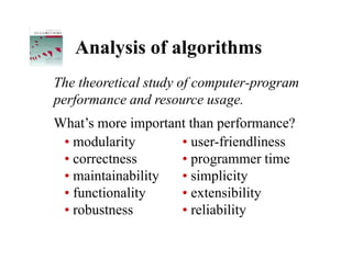
  • 5. Analysis of algorithms The theoretical study of computer-program performance and resource usage. What’s more important than performance? • modularity • user-friendliness • correctness • programmer time • maintainability • simplicity • functionality • extensibility • robustness • reliability
  • 6. Why study algorithms and performance? • Algorithms help us to understand scalability. • Performance often draws the line between what is feasible and what is impossible. • Algorithmic mathematics provides a language for talking about program behavior. • Performance is the currency of computing. • The lessons of program performance generalize to other computing resources. • Speed is fun!
  • 7. The problem of sorting Input: sequence a1, a2, …, an of numbers. Output: permutation a'1, a'2, …, a'n such that a'1  a'2 …  a'n . Example: Input: 8 2 4 9 3 6 Output: 2 3 4 6 8 9
  • 8. Insertion sort INSERTION-SORT (A, n) A[1 . . n] for j ← 2 to n do key ← A[ j] i←j–1 “pseudocode” while i > 0 and A[i] > key do A[i+1] ← A[i] i←i–1 A[i+1] = key
  • 9. Insertion sort INSERTION-SORT (A, n) A[1 . . n] for j ← 2 to n do key ← A[ j] i←j–1 “pseudocode” while i > 0 and A[i] > key do A[i+1] ← A[i] i←i–1 A[i+1] = key 1 i j n A: key sorted
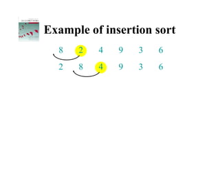
  • 10. Example of insertion sort 8 2 4 9 3 6
  • 11. Example of insertion sort 8 2 4 9 3 6
  • 12. Example of insertion sort 8 2 4 9 3 6 2 8 4 9 3 6
  • 13. Example of insertion sort 8 2 4 9 3 6 2 8 4 9 3 6
  • 14. Example of insertion sort 8 2 4 9 3 6 2 8 4 9 3 6 2 4 8 9 3 6
  • 15. Example of insertion sort 8 2 4 9 3 6 2 8 4 9 3 6 2 4 8 9 3 6
  • 16. Example of insertion sort 8 2 4 9 3 6 2 8 4 9 3 6 2 4 8 9 3 6 2 4 8 9 3 6
  • 17. Example of insertion sort 8 2 4 9 3 6 2 8 4 9 3 6 2 4 8 9 3 6 2 4 8 9 3 6
  • 18. Example of insertion sort 8 2 4 9 3 6 2 8 4 9 3 6 2 4 8 9 3 6 2 4 8 9 3 6 2 3 4 8 9 6
  • 19. Example of insertion sort 8 2 4 9 3 6 2 8 4 9 3 6 2 4 8 9 3 6 2 4 8 9 3 6 2 3 4 8 9 6
  • 20. Example of insertion sort 8 2 4 9 3 6 2 8 4 9 3 6 2 4 8 9 3 6 2 4 8 9 3 6 2 3 4 8 9 6 2 3 4 6 8 9 done
  • 21. Running time • The running time depends on the input: an already sorted sequence is easier to sort. • Parameterize the running time by the size of the input, since short sequences are easier to sort than long ones. • Generally, we seek upper bounds on the running time, because everybody likes a guarantee.
  • 22. Kinds of analyses Worst-case: (usually) • T(n) = maximum time of algorithm on any input of size n. Average-case: (sometimes) • T(n) = expected time of algorithm over all inputs of size n. • Need assumption of statistical distribution of inputs. Best-case: (bogus) • Cheat with a slow algorithm that works fast on some input.
  • 23. Machine-independent time What is insertion sort’s worst-case time? • It depends on the speed of our computer: • relative speed (on the same machine), • absolute speed (on different machines). BIG IDEA: • Ignore machine-dependent constants. • Look at growth of T(n) as n → ∞ . “Asymptotic Analysis”
  • 24. -notation Math: (g(n)) = { f (n) : there exist positive constants c1, c2, and n0 such that 0  c1 g(n)  f (n)  c2 g(n) for all n  n0 } Engineering: • Drop low-order terms; ignore leading constants. • Example: 3n3 + 90n2 – 5n + 6046 = (n3)
  • 25. Asymptotic performance When n gets large enough, a (n2) algorithm always beats a (n3) algorithm. • We shouldn’t ignore asymptotically slower algorithms, however. • Real-world design situations often call for a T(n) careful balancing of engineering objectives. • Asymptotic analysis is a useful tool to help to n n0 structure our thinking.
  • 26. Insertion sort analysis Worst case: Input reverse sorted. n T ( n)   ( j )  n 2  [arithmetic series] j 2 Average case: All permutations equally likely. n T ( n)   ( j / 2)  n 2  j 2 Is insertion sort a fast sorting algorithm? • Moderately so, for small n. • Not at all, for large n.
  • 27. Merge sort MERGE-SORT A[1 . . n] 1. If n = 1, done. 2. Recursively sort A[ 1 . . n/2 ] and A[ n/2+1 . . n ] . 3. “Merge” the 2 sorted lists. Key subroutine: MERGE
  • 28. Merging two sorted arrays 20 12 13 11 7 9 2 1
  • 29. Merging two sorted arrays 20 12 13 11 7 9 2 1 1
  • 30. Merging two sorted arrays 20 12 20 12 13 11 13 11 7 9 7 9 2 1 2 1
  • 31. Merging two sorted arrays 20 12 20 12 13 11 13 11 7 9 7 9 2 1 2 1 2
  • 32. Merging two sorted arrays 20 12 20 12 20 12 13 11 13 11 13 11 7 9 7 9 7 9 2 1 2 1 2
  • 33. Merging two sorted arrays 20 12 20 12 20 12 13 11 13 11 13 11 7 9 7 9 7 9 2 1 2 1 2 7
  • 34. Merging two sorted arrays 20 12 20 12 20 12 20 12 13 11 13 11 13 11 13 11 7 9 7 9 7 9 9 2 1 2 1 2 7
  • 35. Merging two sorted arrays 20 12 20 12 20 12 20 12 13 11 13 11 13 11 13 11 7 9 7 9 7 9 9 2 1 2 1 2 7 9
  • 36. Merging two sorted arrays 20 12 20 12 20 12 20 12 20 12 13 11 13 11 13 11 13 11 13 11 7 9 7 9 7 9 9 2 1 2 1 2 7 9
  • 37. Merging two sorted arrays 20 12 20 12 20 12 20 12 20 12 13 11 13 11 13 11 13 11 13 11 7 9 7 9 7 9 9 2 1 2 1 2 7 9 11
  • 38. Merging two sorted arrays 20 12 20 12 20 12 20 12 20 12 20 12 13 11 13 11 13 11 13 11 13 11 13 7 9 7 9 7 9 9 2 1 2 1 2 7 9 11
  • 39. Merging two sorted arrays 20 12 20 12 20 12 20 12 20 12 20 12 13 11 13 11 13 11 13 11 13 11 13 7 9 7 9 7 9 9 2 1 2 1 2 7 9 11 12
  • 40. Merging two sorted arrays 20 12 20 12 20 12 20 12 20 12 20 12 13 11 13 11 13 11 13 11 13 11 13 7 9 7 9 7 9 9 2 1 2 1 2 7 9 11 12 Time = (n) to merge a total of n elements (linear time).
  • 41. Analyzing merge sort T(n) MERGE-SORT A[1 . . n] (1) 1. If n = 1, done. 2T(n/2) 2. Recursively sort A[ 1 . . n/2 ] Abuse and A[ n/2+1 . . n ] . (n) 3. “Merge” the 2 sorted lists Sloppiness: Should be T( n/2 ) + T( n/2 ) , but it turns out not to matter asymptotically.
  • 42. Recurrence for merge sort (1) if n = 1; T(n) = 2T(n/2) + (n) if n > 1. • We shall usually omit stating the base case when T(n) = (1) for sufficiently small n, but only when it has no effect on the asymptotic solution to the recurrence. • CLRS and Lecture 2 provide several ways to find a good upper bound on T(n).
  • 43. Recursion tree Solve T(n) = 2T(n/2) + cn, where c > 0 is constant.
  • 44. Recursion tree Solve T(n) = 2T(n/2) + cn, where c > 0 is constant. T(n)
  • 45. Recursion tree Solve T(n) = 2T(n/2) + cn, where c > 0 is constant. cn T(n/2) T(n/2)
  • 46. Recursion tree Solve T(n) = 2T(n/2) + cn, where c > 0 is constant. cn cn/2 cn/2 T(n/4) T(n/4) T(n/4) T(n/4)
  • 47. Recursion tree Solve T(n) = 2T(n/2) + cn, where c > 0 is constant. cn cn/2 cn/2 cn/4 cn/4 cn/4 cn/4 (1)
  • 48. Recursion tree Solve T(n) = 2T(n/2) + cn, where c > 0 is constant. cn cn/2 cn/2 h = lg n cn/4 cn/4 cn/4 cn/4 (1)
  • 49. Recursion tree Solve T(n) = 2T(n/2) + cn, where c > 0 is constant. cn cn cn/2 cn/2 h = lg n cn/4 cn/4 cn/4 cn/4 (1)
  • 50. Recursion tree Solve T(n) = 2T(n/2) + cn, where c > 0 is constant. cn cn cn/2 cn/2 cn h = lg n cn/4 cn/4 cn/4 cn/4 (1)
  • 51. Recursion tree Solve T(n) = 2T(n/2) + cn, where c > 0 is constant. cn cn cn/2 cn/2 cn h = lg n cn/4 cn/4 cn/4 cn/4 cn … (1)
  • 52. Recursion tree Solve T(n) = 2T(n/2) + cn, where c > 0 is constant. cn cn cn/2 cn/2 cn h = lg n cn/4 cn/4 cn/4 cn/4 cn … (1) #leaves = n (n)
  • 53. Recursion tree Solve T(n) = 2T(n/2) + cn, where c > 0 is constant. cn cn cn/2 cn/2 cn h = lg n cn/4 cn/4 cn/4 cn/4 cn … (1) #leaves = n (n) Total (n lg n)
  • 54. Conclusions • (n lg n) grows more slowly than (n2). • Therefore, merge sort asymptotically beats insertion sort in the worst case. • In practice, merge sort beats insertion sort for n > 30 or so. • Go test it out for yourself!