


![Inference
Supervised learning is usually concerned with the two following inference
problems:
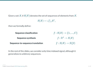
Classi cation: Given , for
, we want to estimate for any new ,
Regression: Given , for , we want
to estimate for any new ,
(x , y ) ∈ X × Y = R × {1, ..., C}
i i
p
i = 1, ..., N x
arg P(Y = y∣X = x).
y
max
(x , y ) ∈ X × Y = R × R
i i
p
i = 1, ..., N
x
E Y ∣X = x .
[ ]
33 / 65](https://image.slidesharecdn.com/639ppt-240602065258-f21a578e/85/639-PPT-46-320.jpg)


![Let denote the hypothesis space, i.e. the set of all functions than can be
produced by the chosen learning algorithm.
We are looking for a function with a small expected risk (or generalization
error)
This means that for a given data generating distribution and for a
given hypothesis space , the optimal model is
F f
f ∈ F
R(f) = E ℓ(y, f(x)) .
(x,y)∼P(X,Y ) [ ]
P(X, Y )
F
f = arg R(f).
∗
f∈F
min
38 / 65](https://image.slidesharecdn.com/639ppt-240602065258-f21a578e/85/639-PPT-51-320.jpg)


![Polynomial regression
Consider the joint probability distribution induced by the data
generating process
where , and is an unknown polynomial of degree 3.
P(X, Y )
(x, y) ∼ P(X, Y ) ⇔ x ∼ U[−10; 10], ϵ ∼ N (0, σ ), y = g(x) + ϵ
2
x ∈ R y ∈ R g
41 / 65](https://image.slidesharecdn.com/639ppt-240602065258-f21a578e/85/639-PPT-54-320.jpg)

![For this regression problem, we use the squared error loss
to measure how wrong the predictions are.
Therefore, our goal is to nd the best value such
ℓ(y, f(x; w)) = (y − f(x; w))2
w∗
w∗ = arg R(w)
w
min
= arg E (y − f(x; w))
w
min (x,y)∼P(X,Y ) [ 2
]
43 / 65](https://image.slidesharecdn.com/639ppt-240602065258-f21a578e/85/639-PPT-56-320.jpg)


![Bias-variance decomposition
Consider a xed point and the prediction of the empirical risk
minimizer at .
Then the local expected risk of is
where
is the local expected risk of the Bayes model. This term cannot be
reduced.
represents the discrepancy between and .
x = f (x)
Y
^ ∗
d
x
f∗
d
R(f ∣x)
∗
d
= E (y − f (x))
y∼P(Y ∣x) [ ∗
d 2
]
= E (y − f (x) + f (x) − f (x))
y∼P(Y ∣x) [ B B ∗
d 2
]
= E (y − f (x)) + E (f (x) − f (x))
y∼P(Y ∣x) [ B
2
] y∼P(Y ∣x) [ B ∗
d 2
]
= R(f ∣x) + (f (x) − f (x))
B B ∗
d 2
R(f ∣x)
B
(f (x) − f (x))
B ∗
d 2
fB f∗
d
60 / 65](https://image.slidesharecdn.com/639ppt-240602065258-f21a578e/85/639-PPT-82-320.jpg)


![Formally, the expected local expected risk yields to:
This decomposition is known as the bias-variance decomposition.
The noise term quantities the irreducible part of the expected risk.
The bias term measures the discrepancy between the average model and the
Bayes model.
The variance term quantities the variability of the predictions.
E R(f ∣x)
d [ ∗
d
]
= E R(f ∣x) + (f (x) − f (x))
d [ B B ∗
d 2
]
= R(f ∣x) + E (f (x) − f (x))
B d [ B ∗
d 2
]
= + +
noise(x)
R(f ∣x)
B
bias (x)
2
(f (x) − E f (x) )
B d [ ∗
d
] 2
var(x)
E (E f (x) − f (x))
d [ d [ ∗
d
] ∗
d 2
]
63 / 65](https://image.slidesharecdn.com/639ppt-240602065258-f21a578e/85/639-PPT-89-320.jpg)


![We have,
This loss is an instance of the cross-entropy
for and .
arg P(d∣w, b)
w,b
max
= arg P(Y = y ∣x , w, b)
w,b
max
x ,y ∈d
i i
∏ i i
= arg σ(w x + b) (1 − σ(w x + b))
w,b
max
x ,y ∈d
i i
∏ T
i
yi T
i
1−yi
= arg
w,b
min
L(w,b)= ℓ(y , (x ;w,b))
∑i i y
^ i
−y log σ(w x + b) − (1 − y ) log(1 − σ(w x + b))
x ,y ∈d
i i
∑ i
T
i i
T
i
H(p, q) = E [− log q]
p
p = Y ∣xi q = ∣x
Y
^ i
21 / 61](https://image.slidesharecdn.com/639ppt-240602065258-f21a578e/85/639-PPT-116-320.jpg)


![Why is stochastic gradient descent still a good idea?
Informally, averaging the update
over all choices restores batch gradient descent.
Formally, if the gradient estimate is unbiased, e.g., if
then the formal convergence of SGD can be proved, under appropriate
assumptions (see references).
Interestingly, if training examples are received and used in an
online fashion, then SGD directly minimizes the expected risk.
θ = θ − γ∇ℓ(y , f(x ; θ ))
t+1 t i(t+1) i(t+1) t
i(t + 1)
E [∇ℓ(y , f(x ; θ ))]
i(t+1) i(t+1) i(t+1) t = ∇ℓ(y , f(x ; θ ))
N
1
x ,y ∈d
i i
∑ i i t
= ∇L(θ )
t
x , y ∼ P
i i X,Y
32 / 61](https://image.slidesharecdn.com/639ppt-240602065258-f21a578e/85/639-PPT-146-320.jpg)
![When decomposing the excess error in terms of approximation, estimation and
optimization errors, stochastic algorithms yield the best generalization
performance (in terms of expected risk) despite being the worst optimization
algorithms (in terms of empirical risk) (Bottou, 2011).
E R( ) − R(f )
[ f
~
∗
d
B ]
= E R(f ) − R(f ) + E R(f ) − R(f ) + E R( ) − R(f )
[ ∗ B ] [ ∗
d
∗ ] [ f
~
∗
d
∗
d
]
= E + E + E
app est opt
33 / 61](https://image.slidesharecdn.com/639ppt-240602065258-f21a578e/85/639-PPT-147-320.jpg)


![Classi cation
For binary classi cation, the width of the last layer is set to , which
results in a single output that models the probability
.
For multi-class classi cation, the sigmoid action in the last layer can be
generalized to produce a (normalized) vector of probability
estimates .
This activation is the function, where its -th output is de ned as
for .
q L 1
h ∈ [0, 1]
L
P(Y = 1∣x)
σ
h ∈ [0, 1]
L
C
P(Y = i∣x)
Softmax i
Softmax(z) = ,
i
exp(z )
∑j=1
C
j
exp(z )
i
i = 1, ..., C
37 / 61](https://image.slidesharecdn.com/639ppt-240602065258-f21a578e/85/639-PPT-151-320.jpg)


!["If we show the perceptron a stimulus, say a square, and associate a response to that
square, this response will immediately generalize perfectly to all transforms of the
square under the transformation group [...]."
This is quite similar to Hubel and Wiesel's simple and complex cells!
―――
Credits: Frank Rosenblatt, Principle of Neurodynamics, 1961. 9 / 71](https://image.slidesharecdn.com/639ppt-240602065258-f21a578e/85/639-PPT-197-320.jpg)


![Convolutions
For one-dimensional tensors, given an input vector and a convolutional
kernel , the discrete convolution is a vector of size
such that
Technically, denotes the cross-correlation operator.
However, most machine learning libraries call it convolution.
x ∈ RW
u ∈ Rw
u ⋆ x W − w + 1
(u ⋆ x)[i] = u x .
m=0
∑
w−1
m m+i
⋆
24 / 71](https://image.slidesharecdn.com/639ppt-240602065258-f21a578e/85/639-PPT-212-320.jpg)


![The nal output is a 2D tensor of size
called the output feature map and such that:
where and are shared parameters to learn.
convolutions can be applied in the same way to produce a
feature map, where is the depth.
o (H − h + 1) × (W − w + 1)
oj,i = b + (u ⋆ x )[j, i] = b + u x
j,i
c=0
∑
C−1
c c j,i
c=0
∑
C−1
n=0
∑
h−1
m=0
∑
w−1
c,n,m c,n+j,m+i
u b
D
D × (H − h + 1) × (W − w + 1) D
28 / 71](https://image.slidesharecdn.com/639ppt-240602065258-f21a578e/85/639-PPT-216-320.jpg)


![The most common convolutional network architecture follows the pattern:
where:
indicates repetition;
indicates an optional pooling layer;
(and usually ), , (and usually );
the last fully connected layer holds the output (e.g., the class scores).
INPUT → [[CONV → RELU]*N → POOL?]*M → [FC → RELU]*K → FC
*
POOL?
N ≥ 0 N ≤ 3 M ≥ 0 K ≥ 0 K < 3
42 / 71](https://image.slidesharecdn.com/639ppt-240602065258-f21a578e/85/639-PPT-230-320.jpg)
![Architectures
Some common architectures for convolutional networks following this pattern
include:
, which implements a linear classi er ( ).
, which implements a -layer MLP.
.
.
.
INPUT → FC N = M = K = 0
INPUT → [FC → RELU]∗K → FC K
INPUT → CONV → RELU → FC
INPUT → [CONV → RELU → POOL]*2 → FC → RELU → FC
INPUT → [[CONV → RELU]*2 → POOL]*3 → [FC → RELU]*2 → FC
43 / 71](https://image.slidesharecdn.com/639ppt-240602065258-f21a578e/85/639-PPT-231-320.jpg)


![----------------------------------------------------------------
Layer (type) Output Shape Param #
================================================================
Conv2d-1 [-1, 6, 28, 28] 156
ReLU-2 [-1, 6, 28, 28] 0
MaxPool2d-3 [-1, 6, 14, 14] 0
Conv2d-4 [-1, 16, 10, 10] 2,416
ReLU-5 [-1, 16, 10, 10] 0
MaxPool2d-6 [-1, 16, 5, 5] 0
Conv2d-7 [-1, 120, 1, 1] 48,120
ReLU-8 [-1, 120, 1, 1] 0
Linear-9 [-1, 84] 10,164
ReLU-10 [-1, 84] 0
Linear-11 [-1, 10] 850
LogSoftmax-12 [-1, 10] 0
================================================================
Total params: 61,706
Trainable params: 61,706
Non-trainable params: 0
----------------------------------------------------------------
Input size (MB): 0.00
Forward/backward pass size (MB): 0.11
Params size (MB): 0.24
Estimated Total Size (MB): 0.35
----------------------------------------------------------------
46 / 71](https://image.slidesharecdn.com/639ppt-240602065258-f21a578e/85/639-PPT-234-320.jpg)

![----------------------------------------------------------------
Layer (type) Output Shape Param #
================================================================
Conv2d-1 [-1, 64, 55, 55] 23,296
ReLU-2 [-1, 64, 55, 55] 0
MaxPool2d-3 [-1, 64, 27, 27] 0
Conv2d-4 [-1, 192, 27, 27] 307,392
ReLU-5 [-1, 192, 27, 27] 0
MaxPool2d-6 [-1, 192, 13, 13] 0
Conv2d-7 [-1, 384, 13, 13] 663,936
ReLU-8 [-1, 384, 13, 13] 0
Conv2d-9 [-1, 256, 13, 13] 884,992
ReLU-10 [-1, 256, 13, 13] 0
Conv2d-11 [-1, 256, 13, 13] 590,080
ReLU-12 [-1, 256, 13, 13] 0
MaxPool2d-13 [-1, 256, 6, 6] 0
Dropout-14 [-1, 9216] 0
Linear-15 [-1, 4096] 37,752,832
ReLU-16 [-1, 4096] 0
Dropout-17 [-1, 4096] 0
Linear-18 [-1, 4096] 16,781,312
ReLU-19 [-1, 4096] 0
Linear-20 [-1, 1000] 4,097,000
================================================================
Total params: 61,100,840
Trainable params: 61,100,840
Non-trainable params: 0
----------------------------------------------------------------
Input size (MB): 0.57
Forward/backward pass size (MB): 8.31
Params size (MB): 233.08
Estimated Total Size (MB): 241.96
----------------------------------------------------------------
48 / 71](https://image.slidesharecdn.com/639ppt-240602065258-f21a578e/85/639-PPT-236-320.jpg)

![----------------------------------------------------------------
Layer (type) Output Shape Param #
================================================================
Conv2d-1 [-1, 64, 224, 224] 1,792
ReLU-2 [-1, 64, 224, 224] 0
Conv2d-3 [-1, 64, 224, 224] 36,928
ReLU-4 [-1, 64, 224, 224] 0
MaxPool2d-5 [-1, 64, 112, 112] 0
Conv2d-6 [-1, 128, 112, 112] 73,856
ReLU-7 [-1, 128, 112, 112] 0
Conv2d-8 [-1, 128, 112, 112] 147,584
ReLU-9 [-1, 128, 112, 112] 0
MaxPool2d-10 [-1, 128, 56, 56] 0
Conv2d-11 [-1, 256, 56, 56] 295,168
ReLU-12 [-1, 256, 56, 56] 0
Conv2d-13 [-1, 256, 56, 56] 590,080
ReLU-14 [-1, 256, 56, 56] 0
Conv2d-15 [-1, 256, 56, 56] 590,080
ReLU-16 [-1, 256, 56, 56] 0
MaxPool2d-17 [-1, 256, 28, 28] 0
Conv2d-18 [-1, 512, 28, 28] 1,180,160
ReLU-19 [-1, 512, 28, 28] 0
Conv2d-20 [-1, 512, 28, 28] 2,359,808
ReLU-21 [-1, 512, 28, 28] 0
Conv2d-22 [-1, 512, 28, 28] 2,359,808
ReLU-23 [-1, 512, 28, 28] 0
MaxPool2d-24 [-1, 512, 14, 14] 0
Conv2d-25 [-1, 512, 14, 14] 2,359,808
ReLU-26 [-1, 512, 14, 14] 0
Conv2d-27 [-1, 512, 14, 14] 2,359,808
ReLU-28 [-1, 512, 14, 14] 0
Conv2d-29 [-1, 512, 14, 14] 2,359,808
ReLU-30 [-1, 512, 14, 14] 0
MaxPool2d-31 [-1, 512, 7, 7] 0
Linear-32 [-1, 4096] 102,764,544
ReLU-33 [-1, 4096] 0
Dropout-34 [-1, 4096] 0
Linear-35 [-1, 4096] 16,781,312
ReLU-36 [-1, 4096] 0
Dropout-37 [-1, 4096] 0
Linear-38 [-1, 1000] 4,097,000
================================================================
Total params: 138,357,544
Trainable params: 138,357,544
Non-trainable params: 0
----------------------------------------------------------------
Input size (MB): 0.57
Forward/backward pass size (MB): 218.59
Params size (MB): 527.79
Estimated Total Size (MB): 746.96
----------------------------------------------------------------
51 / 71](https://image.slidesharecdn.com/639ppt-240602065258-f21a578e/85/639-PPT-239-320.jpg)


![----------------------------------------------------------------
Layer (type) Output Shape Param #
================================================================
Conv2d-1 [-1, 64, 112, 112] 9,408
BatchNorm2d-2 [-1, 64, 112, 112] 128
ReLU-3 [-1, 64, 112, 112] 0
MaxPool2d-4 [-1, 64, 56, 56] 0
Conv2d-5 [-1, 64, 56, 56] 4,096
BatchNorm2d-6 [-1, 64, 56, 56] 128
ReLU-7 [-1, 64, 56, 56] 0
Conv2d-8 [-1, 64, 56, 56] 36,864
BatchNorm2d-9 [-1, 64, 56, 56] 128
ReLU-10 [-1, 64, 56, 56] 0
Conv2d-11 [-1, 256, 56, 56] 16,384
BatchNorm2d-12 [-1, 256, 56, 56] 512
Conv2d-13 [-1, 256, 56, 56] 16,384
BatchNorm2d-14 [-1, 256, 56, 56] 512
ReLU-15 [-1, 256, 56, 56] 0
Bottleneck-16 [-1, 256, 56, 56] 0
Conv2d-17 [-1, 64, 56, 56] 16,384
BatchNorm2d-18 [-1, 64, 56, 56] 128
ReLU-19 [-1, 64, 56, 56] 0
Conv2d-20 [-1, 64, 56, 56] 36,864
BatchNorm2d-21 [-1, 64, 56, 56] 128
ReLU-22 [-1, 64, 56, 56] 0
Conv2d-23 [-1, 256, 56, 56] 16,384
BatchNorm2d-24 [-1, 256, 56, 56] 512
ReLU-25 [-1, 256, 56, 56] 0
Bottleneck-26 [-1, 256, 56, 56] 0
Conv2d-27 [-1, 64, 56, 56] 16,384
BatchNorm2d-28 [-1, 64, 56, 56] 128
ReLU-29 [-1, 64, 56, 56] 0
Conv2d-30 [-1, 64, 56, 56] 36,864
BatchNorm2d-31 [-1, 64, 56, 56] 128
ReLU-32 [-1, 64, 56, 56] 0
Conv2d-33 [-1, 256, 56, 56] 16,384
BatchNorm2d-34 [-1, 256, 56, 56] 512
ReLU-35 [-1, 256, 56, 56] 0
Bottleneck-36 [-1, 256, 56, 56] 0
Conv2d-37 [-1, 128, 56, 56] 32,768
BatchNorm2d-38 [-1, 128, 56, 56] 256
ReLU-39 [-1, 128, 56, 56] 0
Conv2d-40 [-1, 128, 28, 28] 147,456
BatchNorm2d-41 [-1, 128, 28, 28] 256
ReLU-42 [-1, 128, 28, 28] 0
Conv2d-43 [-1, 512, 28, 28] 65,536
BatchNorm2d-44 [-1, 512, 28, 28] 1,024
Conv2d-45 [-1, 512, 28, 28] 131,072
BatchNorm2d-46 [-1, 512, 28, 28] 1,024
ReLU-47 [-1, 512, 28, 28] 0
Bottleneck-48 [-1, 512, 28, 28] 0
Conv2d-49 [-1, 128, 28, 28] 65,536
BatchNorm2d-50 [-1, 128, 28, 28] 256
ReLU-51 [-1, 128, 28, 28] 0
Conv2d-52 [-1, 128, 28, 28] 147,456
BatchNorm2d-53 [-1, 128, 28, 28] 256
...
...
Bottleneck-130 [-1, 1024, 14, 14] 0
Conv2d-131 [-1, 256, 14, 14] 262,144
BatchNorm2d-132 [-1, 256, 14, 14] 512
ReLU-133 [-1, 256, 14, 14] 0
Conv2d-134 [-1, 256, 14, 14] 589,824
BatchNorm2d-135 [-1, 256, 14, 14] 512
ReLU-136 [-1, 256, 14, 14] 0
Conv2d-137 [-1, 1024, 14, 14] 262,144
BatchNorm2d-138 [-1, 1024, 14, 14] 2,048
ReLU-139 [-1, 1024, 14, 14] 0
Bottleneck-140 [-1, 1024, 14, 14] 0
Conv2d-141 [-1, 512, 14, 14] 524,288
BatchNorm2d-142 [-1, 512, 14, 14] 1,024
ReLU-143 [-1, 512, 14, 14] 0
Conv2d-144 [-1, 512, 7, 7] 2,359,296
BatchNorm2d-145 [-1, 512, 7, 7] 1,024
ReLU-146 [-1, 512, 7, 7] 0
Conv2d-147 [-1, 2048, 7, 7] 1,048,576
BatchNorm2d-148 [-1, 2048, 7, 7] 4,096
Conv2d-149 [-1, 2048, 7, 7] 2,097,152
BatchNorm2d-150 [-1, 2048, 7, 7] 4,096
ReLU-151 [-1, 2048, 7, 7] 0
Bottleneck-152 [-1, 2048, 7, 7] 0
Conv2d-153 [-1, 512, 7, 7] 1,048,576
BatchNorm2d-154 [-1, 512, 7, 7] 1,024
ReLU-155 [-1, 512, 7, 7] 0
Conv2d-156 [-1, 512, 7, 7] 2,359,296
BatchNorm2d-157 [-1, 512, 7, 7] 1,024
ReLU-158 [-1, 512, 7, 7] 0
Conv2d-159 [-1, 2048, 7, 7] 1,048,576
BatchNorm2d-160 [-1, 2048, 7, 7] 4,096
ReLU-161 [-1, 2048, 7, 7] 0
Bottleneck-162 [-1, 2048, 7, 7] 0
Conv2d-163 [-1, 512, 7, 7] 1,048,576
BatchNorm2d-164 [-1, 512, 7, 7] 1,024
ReLU-165 [-1, 512, 7, 7] 0
Conv2d-166 [-1, 512, 7, 7] 2,359,296
BatchNorm2d-167 [-1, 512, 7, 7] 1,024
ReLU-168 [-1, 512, 7, 7] 0
Conv2d-169 [-1, 2048, 7, 7] 1,048,576
BatchNorm2d-170 [-1, 2048, 7, 7] 4,096
ReLU-171 [-1, 2048, 7, 7] 0
Bottleneck-172 [-1, 2048, 7, 7] 0
AvgPool2d-173 [-1, 2048, 1, 1] 0
Linear-174 [-1, 1000] 2,049,000
================================================================
Total params: 25,557,032
Trainable params: 25,557,032
Non-trainable params: 0
----------------------------------------------------------------
Input size (MB): 0.57
Forward/backward pass size (MB): 286.56
Params size (MB): 97.49
Estimated Total Size (MB): 384.62
----------------------------------------------------------------
54 / 71](https://image.slidesharecdn.com/639ppt-240602065258-f21a578e/85/639-PPT-242-320.jpg)


![Maximum response samples
Convolutional networks can be inspected by looking for input images that
maximize the activation of a chosen convolutional kernel at layer and
index in the layer lter bank.
Such images can be found by gradient ascent on the input space:
x
h (x)
ℓ,d u ℓ
d
L (x)
ℓ,d
x0
xt+1
= ∣∣h (x)∣∣
ℓ,d 2
∼ U[0, 1]C×H×W
= x + γ∇ L (x )
t x ℓ,d t
61 / 71](https://image.slidesharecdn.com/639ppt-240602065258-f21a578e/85/639-PPT-249-320.jpg)


![The tradeoffs of learning
When decomposing the excess error in terms of approximation, estimation and
optimization errors, stochastic algorithms yield the best generalization
performance (in terms of expected risk) despite being the worst optimization
algorithms (in terms of empirical risk) (Bottou, 2011).
E R( ) − R(f )
[ f
~
∗
d
B ]
= E R(f ) − R(f ) + E R(f ) − R(f ) + E R( ) − R(f )
[ ∗ B ] [ ∗
d
∗ ] [ f
~
∗
d
∗
d
]
= E + E + E
app est opt
21 / 56](https://image.slidesharecdn.com/639ppt-240602065258-f21a578e/85/639-PPT-281-320.jpg)


![Let us assume that
we are in a linear regime at initialization (e.g., the positive part of a ReLU or
the middle of a sigmoid),
weights are initialized independently,
biases are initialized to be ,
input feature variances are the same, which we denote as .
Then, the variance of the activation of unit in layer is
where is the width of layer and for all .
wij
l
bl 0
V[x]
hi
l
i l
V h
[ i
l
] = V w h
[
j=0
∑
q −1
l−1
ij
l
j
l−1
]
= V w V h
j=0
∑
q −1
l−1
[ ij
l
] [ j
l−1
]
ql l h = x
j
0
j j = 0, ..., p − 1
38 / 56](https://image.slidesharecdn.com/639ppt-240602065258-f21a578e/85/639-PPT-298-320.jpg)
![If we further assume that weights at layer share the same variance
and that the variance of the activations in the previous layer are the same, then
we can drop the indices and write
Therefore, the variance of the activations is preserved across layers when
This condition is enforced in LeCun's uniform initialization, which is de ned as
wij
l
l V w
[ l
]
V h = q V w V h .
[ l
] l−1 [ l
] [ l−1
]
V w = ∀l.
[ l
]
ql−1
1
w ∼ U − , .
ij
l
[
ql−1
3
ql−1
3
]
39 / 56](https://image.slidesharecdn.com/639ppt-240602065258-f21a578e/85/639-PPT-299-320.jpg)
![Controlling for the variance in the backward pass
A similar idea can be applied to ensure that the gradients ow in the backward
pass (without vanishing nor exploding), by maintaining the variance of the
gradient with respect to the activations xed across layers.
Under the same assumptions as before,
V [
dhi
l
dy
^
] = V [
j=0
∑
q −1
l+1
dhj
l+1
dy
^
∂hi
l
∂hj
l+1
]
= V w
[
j=0
∑
q −1
l+1
dhj
l+1
dy
^
j,i
l+1
]
= V V w
j=0
∑
q −1
l+1
[
dhj
l+1
dy
^
] [ ji
l+1
]
40 / 56](https://image.slidesharecdn.com/639ppt-240602065258-f21a578e/85/639-PPT-300-320.jpg)
![If we further assume that
the gradients of the activations at layer share the same variance
the weights at layer share the same variance ,
then we can drop the indices and write
Therefore, the variance of the gradients with respect to the activations is
preserved across layers when
l
l + 1 V w
[ l+1
]
V = q V V w .
[
dhl
dy
^
] l+1 [
dhl+1
dy
^
] [ l+1
]
V w = ∀l.
[ l
]
ql
1
41 / 56](https://image.slidesharecdn.com/639ppt-240602065258-f21a578e/85/639-PPT-301-320.jpg)
![Xavier initialization
We have derived two different conditions on the variance of ,
.
A compromise is the Xavier initialization, which initializes randomly from a
distribution with variance
For example, normalized initialization is de ned as
wl
V w =
[ l
] ql−1
1
V w =
[ l
] ql
1
wl
V w = = .
[ l
]
2
q +q
l−1 l
1
q + q
l−1 l
2
w ∼ U − , .
ij
l
[
q + q
l−1 l
6
q + q
l−1 l
6
]
42 / 56](https://image.slidesharecdn.com/639ppt-240602065258-f21a578e/85/639-PPT-302-320.jpg)


![Data normalization
Previous weight initialization strategies rely on preserving the activation
variance constant across layers, under the initial assumption that the input
feature variances are the same.
That is,
for all pairs of features .
V x = V x ≜ V x
[ i] [ j ] [ ]
i, j
―――
Credits: Francois Fleuret, EE559 Deep Learning, EPFL. 46 / 56](https://image.slidesharecdn.com/639ppt-240602065258-f21a578e/85/639-PPT-306-320.jpg)


![xt
ht
ct
⊙ +
σ σ
ft c̄t
ht−1
ct−1
σ tanh
it
⊙
ot ⊙
tanh
ft = σ W [h , x ] + b
( f
T
t−1 t f )
29 / 69](https://image.slidesharecdn.com/639ppt-240602065258-f21a578e/85/639-PPT-346-320.jpg)
![xt
ht
ct
⊙ +
σ σ
ft c̄t
ht−1
ct−1
σ tanh
it
⊙
ot ⊙
tanh
it
c̄t
= σ W [h , x ] + b
( i
T
t−1 t i)
= tanh W [h , x ] + b
( c
T
t−1 t c)
30 / 69](https://image.slidesharecdn.com/639ppt-240602065258-f21a578e/85/639-PPT-347-320.jpg)

![xt
ht
ct
⊙ +
σ σ
ft c̄t
ht−1
ct−1
σ tanh
it
⊙
ot ⊙
tanh
ot
ht
= σ W [h , x ] + b
( o
T
t−1 t o)
= o ⊙ tanh(c )
t t
32 / 69](https://image.slidesharecdn.com/639ppt-240602065258-f21a578e/85/639-PPT-349-320.jpg)


![xt
ht
ht−1
+
σ σ
r t zt
1 −
tanh h̄
¯t
⊙
⊙
⊙
zt
rt
h̄t
ht
= σ W [h , x ] + b
( z
T
t−1 t z)
= σ W [h , x ] + b
( r
T
t−1 t r)
= tanh W [r ⊙ h , x ] + b
( h
T
t t−1 t h)
= (1 − z ) ⊙ h + z ⊙
t h−1 t h̄t
36 / 69](https://image.slidesharecdn.com/639ppt-240602065258-f21a578e/85/639-PPT-353-320.jpg)


![Let be the data distribution over . A good auto-encoder could be
characterized with the reconstruction loss
Given two parameterized mappings and , training consists of
minimizing an empirical estimate of that loss,
p(x) X
E ∣∣x − g ∘ f(x)∣∣ ≈ 0.
x∼p(x) [ 2
]
f(⋅; θ )
f g(⋅; θ )
f
θ = arg ∣∣x − g(f(x , θ ), θ )∣∣ .
θ ,θ
f g
min
N
1
i=1
∑
N
i i f g
2
―――
Credits: Francois Fleuret, EE559 Deep Learning, EPFL. 9 / 70](https://image.slidesharecdn.com/639ppt-240602065258-f21a578e/85/639-PPT-396-320.jpg)
![For example, when the auto-encoder is linear,
with , the reconstruction error reduces to
In this case, an optimal solution is given by PCA.
f : z
g : x
^
= U x
T
= Uz,
U ∈ Rp×k
E ∣∣x − UU x∣∣ .
x∼p(x) [ T 2
]
10 / 70](https://image.slidesharecdn.com/639ppt-240602065258-f21a578e/85/639-PPT-397-320.jpg)


![Formally, we want to minimize
For the same reason as before, the KL divergence cannot be directly minimized
because of the term.
KL(q(z∣x; ν)∣∣p(z∣x)) = E log
q(z∣x;ν) [
p(z∣x)
q(z∣x; ν)
]
= E log q(z∣x; ν) − log p(x, z) + log p(x).
q(z∣x;ν) [ ]
log p(x)
43 / 70](https://image.slidesharecdn.com/639ppt-240602065258-f21a578e/85/639-PPT-430-320.jpg)
![However, we can write
where is called the evidence lower bound objective.
Since does not depend on , it can be considered as a constant, and
minimizing the KL divergence is equivalent to maximizing the evidence lower
bound, while being computationally tractable.
Given a dataset , the nal objective is the sum
.
KL(q(z∣x; ν)∣∣p(z∣x)) = log p(x) −
ELBO(x;ν)
E log p(x, z) − log q(z∣x; ν)
q(z∣x;ν) [ ]
ELBO(x; ν)
log p(x) ν
d = {x ∣i = 1, ..., N}
i
ELBO(x ; ν)
∑{x ∈d}
i i
44 / 70](https://image.slidesharecdn.com/639ppt-240602065258-f21a578e/85/639-PPT-431-320.jpg)
![Remark that
Therefore, maximizing the ELBO:
encourages distributions to place their mass on con gurations of latent
variables that explain the observed data ( rst term);
encourages distributions close to the prior (second term).
ELBO(x; ν) = E log p(x, z) − log q(z∣x; ν)
q(z;∣xν) [ ]
= E log p(x∣z)p(z) − log q(z∣x; ν)
q(z∣x;ν) [ ]
= E log p(x∣z) − KL(q(z∣x; ν)∣∣p(z))
q(z∣x;ν) [ ]
45 / 70](https://image.slidesharecdn.com/639ppt-240602065258-f21a578e/85/639-PPT-432-320.jpg)
![Optimization
We want
We can proceed by gradient ascent, provided we can evaluate .
In general, this gradient is dif cult to compute because the expectation is
unknown and the parameters are parameters of the distribution we
integrate over.
ν∗
= arg ELBO(x; ν)
ν
max
= arg E log p(x, z) − log q(z∣x; ν) .
ν
max q(z∣x;ν) [ ]
∇ ELBO(x; ν)
ν
ν q(z∣x; ν)
46 / 70](https://image.slidesharecdn.com/639ppt-240602065258-f21a578e/85/639-PPT-433-320.jpg)


![As before, we can use variational inference, but to jointly optimize the generative
and the inference networks parameters and .
We want
Given some generative network , we want to put the mass of the latent
variables, by adjusting , such that they explain the observed data, while
remaining close to the prior.
Given some inference network , we want to put the mass of the observed
variables, by adjusting , such that they are well explained by the latent
variables.
θ φ
θ , φ
∗ ∗
= arg ELBO(x; θ, φ)
θ,φ
max
= arg E log p(x, z; θ) − log q(z∣x; φ)
θ,φ
max q(z∣x;φ) [ ]
= arg E log p(x∣z; θ) − KL(q(z∣x; φ)∣∣p(z)).
θ,φ
max q(z∣x;φ) [ ]
θ
φ
φ
θ
51 / 70](https://image.slidesharecdn.com/639ppt-240602065258-f21a578e/85/639-PPT-438-320.jpg)
![Unbiased gradients of the ELBO with respect to the generative model
parameters are simple to obtain:
which can be estimated with Monte Carlo integration.
However, gradients with respect to the inference model parameters are more
dif cult to obtain:
θ
∇ ELBO(x; θ, φ)
θ = ∇ E log p(x, z; θ) − log q(z∣x; φ)
θ q(z∣x;φ) [ ]
= E ∇ (log p(x, z; θ) − log q(z∣x; φ))
q(z∣x;φ) [ θ ]
= E ∇ log p(x, z; θ) ,
q(z∣x;φ) [ θ ]
φ
∇ ELBO(x; θ, φ)
φ = ∇ E log p(x, z; θ) − log q(z∣x; φ)
φ q(z∣x;φ) [ ]
≠ E ∇ (log p(x, z; θ) − log q(z∣x; φ))
q(z∣x;φ) [ φ ]
52 / 70](https://image.slidesharecdn.com/639ppt-240602065258-f21a578e/85/639-PPT-439-320.jpg)
![x
z
f
φ
~q(z ∣ x; φ)
Let us abbreviate
We have
We cannot backpropagate through the stochastic node to compute !
ELBO(x; θ, φ) = E log p(x, z; θ) − log q(z∣x; φ)
q(z∣x;φ) [ ]
= E f(x, z; φ) .
q(z∣x;φ) [ ]
z ∇ f
φ
53 / 70](https://image.slidesharecdn.com/639ppt-240602065258-f21a578e/85/639-PPT-440-320.jpg)


![Given such a change of variable, the ELBO can be rewritten as:
Therefore,
which we can now estimate with Monte Carlo integration.
The last required ingredient is the evaluation of the likelihood given
the change of variable . As long as is invertible, we have:
ELBO(x; θ, φ) = E f(x, z; φ)
q(z∣x;φ) [ ]
= E f(x, g(φ, x, ϵ); φ)
p(ϵ) [ ]
∇ ELBO(x; θ, φ)
φ = ∇ E f(x, g(φ, x, ϵ); φ)
φ p(ϵ) [ ]
= E ∇ f(x, g(φ, x, ϵ); φ) ,
p(ϵ) [ φ ]
q(z∣x; φ)
g g
log q(z∣x; φ) = log p(ϵ) − log det .
∣
∣
∣
∣
(
∂ϵ
∂z
)
∣
∣
∣
∣
56 / 70](https://image.slidesharecdn.com/639ppt-240602065258-f21a578e/85/639-PPT-443-320.jpg)


![Plugging everything together, the objective can be expressed as:
where the KL divergence can be expressed analytically as
which allows to evaluate its derivative without approximation.
ELBO(x; θ, φ) = E log p(x, z; θ) − log q(z∣x; φ)
q(z∣x;φ) [ ]
= E log p(x∣z; θ) − KL(q(z∣x; φ)∣∣p(z))
q(z∣x;φ) [ ]
= E log p(x∣z = g(φ, x, ϵ); θ) − KL(q(z∣x; φ)∣∣p(z))
p(ϵ) [ ]
KL(q(z∣x; φ)∣∣p(z)) = 1 + log(σ (x; φ)) − μ (x; φ) − σ (x; φ) ,
2
1
j=1
∑
J
( j
2
j
2
j
2
)
59 / 70](https://image.slidesharecdn.com/639ppt-240602065258-f21a578e/85/639-PPT-446-320.jpg)


![A two-player game
In generative adversarial networks (GANs), the task of learning a generative
model is expressed as a two-player zero-sum game between two networks.
The rst network is a generator , mapping a latent space
equipped with a prior distribution to the data space, thereby inducing a
distribution
The second network is a classi er trained to
distinguish between true samples and generated samples
.
The central mechanism consists in using supervised learning to guide the learning
of the generative model.
g(⋅; θ) : Z → X
p(z)
x ∼ q(x; θ) ⇔ z ∼ p(z), x = g(z; θ).
d(⋅; ϕ) : X → [0, 1]
x ∼ p(x)
x ∼ q(x; θ)
6 / 82](https://image.slidesharecdn.com/639ppt-240602065258-f21a578e/85/639-PPT-464-320.jpg)
![arg
θ
min
ϕ
max
V (ϕ,θ)
E log d(x; ϕ) + E log(1 − d(g(z; θ); ϕ))
x∼p(x) [ ] z∼p(z) [ ]
7 / 82](https://image.slidesharecdn.com/639ppt-240602065258-f21a578e/85/639-PPT-465-320.jpg)


![Therefore,
where is the Jensen-Shannon divergence.
V (ϕ, θ) = V (ϕ , θ)
θ
min
ϕ
max
θ
min θ
∗
= E log + E log
θ
min x∼p(x) [
q(x; θ) + p(x)
p(x)
] x∼q(x;θ) [
q(x; θ) + p(x)
q(x; θ)
]
= KL p(x)∣∣
θ
min (
2
p(x) + q(x; θ)
)
+ KL q(x; θ)∣∣ − log 4
(
2
p(x) + q(x; θ)
)
= 2 JSD(p(x)∣∣q(x; θ)) − log 4
θ
min
JSD
13 / 82](https://image.slidesharecdn.com/639ppt-240602065258-f21a578e/85/639-PPT-471-320.jpg)


![Return of the Vanishing Gradients
For most non-toy data distributions, the fake samples may be so bad
initially that the response of saturates.
At the limit, when is perfect given the current generator ,
Therefore,
and , thereby halting gradient descent.
x ∼ q(x; θ)
d
d g
d(x; ϕ)
d(x; ϕ)
= 1, ∀x ∼ p(x),
= 0, ∀x ∼ q(x; θ).
V (ϕ, θ) = E log d(x; ϕ) + E log(1 − d(g(z; θ); ϕ)) = 0
x∼p(x) [ ] z∼p(z) [ ]
∇ V (ϕ, θ) = 0
θ
27 / 82](https://image.slidesharecdn.com/639ppt-240602065258-f21a578e/85/639-PPT-485-320.jpg)


![Wasserstein distance
An alternative choice is the Earth mover's distance, which intuitively corresponds
to the minimum mass displacement to transform one distribution into the other.
Then,
p = 1 + 1 + 1
4
1
[1,2] 4
1
[3,4] 2
1
[9,10]
q = 1[5,7]
W (p, q) = 4 × + 2 × + 3 × = 3
1
4
1
4
1
2
1
―――
Credits: Francois Fleuret, EE559 Deep Learning, EPFL. 31 / 82](https://image.slidesharecdn.com/639ppt-240602065258-f21a578e/85/639-PPT-489-320.jpg)
![The Earth mover's distance is also known as the Wasserstein-1 distance and is
de ned as:
where:
denotes the set of all joint distributions whose marginals are
respectively and ;
indicates how much mass must be transported from to in order
to transform the distribution into .
is the L1 norm and represents the cost of moving a unit of
mass from to .
W (p, q) = E ∣∣x − y∣∣
1
γ∈Π(p,q)
inf (x,y)∼γ [ ]
Π(p, q) γ(x, y)
p q
γ(x, y) x y
p q
∣∣ ⋅ ∣∣ ∣∣x − y∣∣
x y
32 / 82](https://image.slidesharecdn.com/639ppt-240602065258-f21a578e/85/639-PPT-490-320.jpg)


![Wasserstein GANs
Given the attractive properties of the Wasserstein-1 distance, Arjovsky et al
(2017) propose to learn a generative model by solving instead:
Unfortunately, the de nition of does not provide with an operational way of
estimating it because of the intractable .
On the other hand, the Kantorovich-Rubinstein duality tells us that
where the supremum is over all the 1-Lipschitz functions . That is,
functions such that
θ = arg W (p(x)∣∣q(x; θ))
∗
θ
min 1
W1
inf
W (p(x)∣∣q(x; θ)) = E f(x) − E f(x)
1
∣∣f∣∣ ≤1
L
sup x∼p(x) [ ] x∼q(x;θ) [ ]
f : X → R
f
∣∣f∣∣ = ≤ 1.
L
x,x′
max
∣∣x − x ∣∣
′
∣∣f(x) − f(x )∣∣
′
35 / 82](https://image.slidesharecdn.com/639ppt-240602065258-f21a578e/85/639-PPT-493-320.jpg)
![For and ,
p = 1 + 1 + 1
4
1
[1,2] 4
1
[3,4] 2
1
[9,10] q = 1[5,7]
W (p, q)
1 = 4 × + 2 × + 3 × = 3
4
1
4
1
2
1
= − = 3
E f(x)
x∼p(x) [ ]
3 × + 1 × + 2 ×
(
4
1
4
1
2
1
)
E f(x)
x∼q(x;θ) [ ]
−1 × − 1 ×
(
2
1
2
1
)
―――
Credits: Francois Fleuret, EE559 Deep Learning, EPFL. 36 / 82](https://image.slidesharecdn.com/639ppt-240602065258-f21a578e/85/639-PPT-494-320.jpg)
![Using this result, the Wasserstein GAN algorithm consists in solving the minimax
problem:
Note that this formulation is very close to the original GANs, except that:
The classi er is replaced by a critic function and
its output is not interpreted through the cross-entropy loss;
There is a strong regularization on the form of . In practice, to ensure 1-
Lipschitzness,
Arjovsky et al (2017) proposeto clip theweights of thecriticat each iteration;
Gulrajani et al (2017) add a regularization term to theloss.
As a result, Wasserstein GANs bene t from:
a meaningful loss metric,
improved stability (no modecollapseis observed).
θ = arg E d(x; ϕ) − E d(x; ϕ)
∗
θ
min
ϕ:∣∣d(⋅;ϕ)∣∣ ≤1
L
max x∼p(x) [ ] x∼q(x;θ) [ ]
d : X → [0, 1] d : X → R
d
37 / 82](https://image.slidesharecdn.com/639ppt-240602065258-f21a578e/85/639-PPT-495-320.jpg)


![Following the notations of Mescheder et al (2018), the training objective for the
two players can be described by an objective function of the form
where the goal of the generator is to minimizes the loss, whereas the
discriminator tries to maximize it.
If , then we recover the original GAN
objective.
if and and if we impose the Lipschitz constraint on , then we
recover Wassterstein GAN.
L(θ, ϕ) = E f(d(g(z; θ); ϕ)) + E f(−d(x; ϕ)) ,
p(z) [ ] p(x) [ ]
f(t) = − log(1 + exp(−t))
f(t) = −t d
42 / 82](https://image.slidesharecdn.com/639ppt-240602065258-f21a578e/85/639-PPT-500-320.jpg)


![Dirac-GAN: Zero-centered gradient penalties
A penalty on the squared norm of the gradients of the discriminator results in the
regularization
The resulting eigenvalues are . Therefore, for , all
eigenvalues have negative real part, hence training is locally convergent!
R (ϕ) = E ∣∣∇ d(x; ϕ)∣∣ .
1
2
γ
x∼p(x) [ x
2
]
{− ± }
2
γ
− f (0)
4
γ ′ 2 γ > 0
―――
Credits: Mescheder et al, Which Training Methods for GANs do actually Converge?, 2018. 52 / 82](https://image.slidesharecdn.com/639ppt-240602065258-f21a578e/85/639-PPT-510-320.jpg)


![We have,
[Q] What if was xed?
arg p(d∣θ, σ )
θ,σ2
max 2
= arg p(y ∣x , θ, σ )
θ,σ2
max
x ,y ∈d
i i
∏ i i
2
= arg exp −
θ,σ2
max
x ,y ∈d
i i
∏
σ
2π
1
(
2σ2
(y − μ(x ))
i i
2
)
= arg + log(σ) + C
θ,σ2
min
x ,y ∈d
i i
∑
2σ2
(y − μ(x ))
i i
2
σ2
18 / 52](https://image.slidesharecdn.com/639ppt-240602065258-f21a578e/85/639-PPT-559-320.jpg)


![The data can be t with a 2-layer network producing point estimates for .
[demo]
y
―――
Credits: David Ha, Mixture Density Networks, 2015. 25 / 52](https://image.slidesharecdn.com/639ppt-240602065258-f21a578e/85/639-PPT-566-320.jpg)
![If we ip and , the network faces issues since for each input, there are
multiple outputs that can work. It produces some sort of average of the correct
values. [demo]
xi yi
―――
Credits: David Ha, Mixture Density Networks, 2015. 26 / 52](https://image.slidesharecdn.com/639ppt-240602065258-f21a578e/85/639-PPT-567-320.jpg)
![A mixture density network models the data correctly, as it predicts for each input
a distribution for the output, rather than a point estimate. [demo]
―――
Credits: David Ha, Mixture Density Networks, 2015. 27 / 52](https://image.slidesharecdn.com/639ppt-240602065258-f21a578e/85/639-PPT-568-320.jpg)


![Variational inference
Variational inference can be used for building an approximation of the
posterior .
As before (see Lecture 6), we can show that minimizing
with respect to the variational parameters , is identical to maximizing the
evidence lower bound objective (ELBO)
q(ω; ν)
p(ω∣X, Y)
KL(q(ω; ν)∣∣p(ω∣X, Y))
ν
ELBO(ν) = E log p(Y∣X, ω) − KL(q(ω; ν)∣∣p(ω)).
q(ω;ν) [ ]
33 / 52](https://image.slidesharecdn.com/639ppt-240602065258-f21a578e/85/639-PPT-574-320.jpg)


![That is, are obtained by setting columns
of to zero with probability .
This is strictly equivalent to dropout, i.e.
removing units from the network with
probability .
Given the previous de nition for , sampling parameters is
done as follows:
Draw binary for each layer and unit .
Compute , where denotes a matrix
composed of the columns .
q = { , ..., }
ω
^ W
^ 1 W
^ L
z ∼ Bernoulli(1 − p)
i,k i k
= M diag([z ] )
W
^ i i i,k k=1
qi
Mi
mi,k
W
^ i
Mi p
p
40 / 52](https://image.slidesharecdn.com/639ppt-240602065258-f21a578e/85/639-PPT-581-320.jpg)


![Uncertainty estimates from dropout
Proper epistemic uncertainty estimates at can be obtained in a principled way
using Monte-Carlo integration:
Draw sets of network parameters from .
Compute the predictions for the networks, .
Approximate the predictive mean and variance as follows:
x
T ω
^t q(ω; ν)
T {f(x; )}
ω
^t t=1
T
E y
p(y∣x,X,Y) [ ]
V y
p(y∣x,X,Y) [ ]
≈ f(x; )
T
1
t=1
∑
T
ω
^t
≈ σ + f(x; ) − y
2
T
1
t=1
∑
T
ω
^t
2
E
^ [ ]2
44 / 52](https://image.slidesharecdn.com/639ppt-240602065258-f21a578e/85/639-PPT-585-320.jpg)


![For a xed value , let us consider the prior distribution of implied by
the prior distributions for the weights and biases.
We have
since and are statistically independent and has zero mean by
hypothesis.
The variance of the contribution of each hidden unit is
which must be nite since is bounded by its activation function.
We de ne , and is the same for all .
x(1)
f(x )
(1)
E[v h (x )] = E[v ]E[h (x )] = 0,
j j
(1)
j j
(1)
vj h (x )
j
(1)
vj
hj
V[v h (x )]
j j
(1)
= E[(v h (x )) ] − E[v h (x )]
j j
(1) 2
j j
(1) 2
= E[v ]E[h (x ) ]
j
2
j
(1) 2
= σ E[h (x ) ],
v
2
j
(1) 2
hj
V (x ) = E[h (x ) ]
(1)
j
(1) 2
j
48 / 52](https://image.slidesharecdn.com/639ppt-240602065258-f21a578e/85/639-PPT-589-320.jpg)

![Accordingly, for , for some xed , the prior converges to a
Gaussian of mean zero and variance as .
For two or more xed values , a similar argument shows that, as
, the joint distribution of the outputs converges to a multivariate
Gaussian with means of zero and covariances of
where and is the same for all .
σ = ω q
v v
−2
1
ωv f(x )
(1)
σ + ω σ V (x )
b
2
v
2
v
2 (1)
q → ∞
x , x , ...
(1) (2)
q → ∞
E[f(x )f(x )]
(1) (2)
= σ + σ E[h (x )h (x )]
b
2
j=1
∑
q
v
2
j
(1)
j
(2)
= σ + ω C(x , x )
b
2
v
2 (1) (2)
C(x , x ) = E[h (x )h (x )]
(1) (2)
j
(1)
j
(2)
j
50 / 52](https://image.slidesharecdn.com/639ppt-240602065258-f21a578e/85/639-PPT-591-320.jpg)


深度学习639页PPT/////////////////////////////
- 1. Deep Learning Spring 2019 Prof. Gilles Louppe g.louppe@uliege.be 1 / 12
- 2. Logistics This course is given by: Theory: Prof. Gilles Louppe (g.louppe@uliege.be) Projects and guidance: Joeri Hermans (joeri.hermans@doct.uliege.be) Matthia Sabatelli (m.sabatelli@uliege.be) AntoineWehenkel (antoine.wehenkel@uliege.be) Feel free to contact any of us for help! 2 / 12
- 4. Materials Slides are available at github.com/glouppe/info8010-deep-learning. In HTML and in PDFs. Posted online the day before the lesson (hopefully). Some lessons are partially adapted from "EE-559 Deep Learning" by Francois Fleuret at EPFL. 4 / 12
- 6. Resources Awesome Deep Learning Awesome Deep Learning papers 6 / 12
- 7. AI at ULiège This course is part of the many other courses available at ULiège and related to AI, including: INFO8006: Introduction to Arti cial Intelligence ELEN0062: Introduction to Machine Learning INFO8010: Deep Learning you are there INFO8003: Optimal decision making for complex problems INFO8004: Advanced Machine Learning INFO0948: Introduction to Intelligent Robotics INFO0049: Knowledge representation ELEN0016: Computer vision DROI8031: Introduction to the law of robots ← 7 / 12
- 8. Outline (Tentative and subject to change!) Lecture 1: Fundamentals of machine learning Lecture 2: Neural networks Lecture 3: Convolutional neural networks Lecture 4: Training neural networks Lecture 5: Recurrent neural networks Lecture 6: Auto-encoders and generative models Lecture 7: Generative adversarial networks Lecture 8: Uncertainty Lecture 9: Adversarial attacks and defenses 8 / 12
- 9. Philosophy Thorough and detailed Understand the foundations and the landscape of deep learning. Be able to write from scratch, debug and run (some) deep learning algorithms. State-of-the-art Introduction to materials new from research ( 5 years old). Understand some of the open questions and challenges in the eld. Practical Fun and challenging course project. ≤ 9 / 12
- 10. Projects Reading assignment Read, summarize and criticize a major scienti c paper in deep learning. Pick one of the following three papers: He, K., Zhang, X., Ren, S., & Sun, J. (2016). Deep residual learning for image recognition. arXiv:1512.03385. Andrychowicz, M., Denil, M., Gomez, S., Hoffman, M. W., Pfau, D., Schaul, T., ... & De Freitas, N. (2016). Learning to learn by gradient descent by gradient descent. arXiv:1606.04474. Zhang, C., Bengio, S., Hardt, M., Recht, B., & Vinyals, O. (2016). Understanding deep learning requires rethinking generalization. arXiv:1611.03530. Deadline: April 5, 2019 at 23:59. 10 / 12
- 11. Project Ambitious project of your choosing. Details to be announced soon. 11 / 12
- 12. Evaluation Exam (50%) Reading assignment (10%) Project (40%) The reading assignment and the project are mandatory for presenting the exam. 12 / 12
- 13. Let's start! 12 / 12
- 14. Deep Learning Lecture 1: Fundamentals of machine learning Prof. Gilles Louppe g.louppe@uliege.be 1 / 65
- 15. Today Set the fundamentals of machine learning. Why learning? Applications and success Statistical learning Supervised learning Empirical riskminimization Under- tting and over- tting Bias-variancedilemma 2 / 65
- 16. Why learning? 3 / 65
- 17. What do you see? How do we do that?! 4 / 65
- 18. Sheepdog or mop? ――― Credits: Karen Zack, 2016. 5 / 65
- 19. Chihuahua or muf n? ――― Credits: Karen Zack. 2016. 6 / 65
- 20. The automatic extraction of semantic information from raw signal is at the core of many applications, such as image recognition speech processing natural language processing robotic control ... and many others. How can we write a computer program that implements that? 7 / 65
- 21. The (human) brain is so good at interpreting visual information that the gap between raw data and its semantic interpretation is dif cult to assess intuitively: This is a mushroom. 8 / 65
- 22. This is a mushroom. 9 / 65
- 23. + + This is a mushroom. 10 / 65
- 24. This is a mushroom. 11 / 65
- 25. Extracting semantic information requires models of high complexity, which cannot be designed by hand. However, one can write a program that learns the task of extracting semantic information. Techniques used in practice consist of: de ning a parametric model with high capacity, optimizing its parameters, by "making it work" on the training data. ――― Credits: Francois Fleuret, EE559 Deep Learning, EPFL. 12 / 65
- 26. This is similar to biological systems for which the model (e.g., brain structure) is DNA-encoded, and parameters (e.g., synaptic weights) are tuned through experiences. Deep learning encompasses software technologies to scale-up to billions of model parameters and as many training examples. ――― Credits: Francois Fleuret, EE559 Deep Learning, EPFL. 13 / 65
- 27. Applications and success 14 / 65
- 28. YOLOv3 YOLOv3 YOLOv3 Watch later Share Real-time object detection (Redmon and Farhadi, 2018) 15 / 65
- 29. ICNet for Real-Time Semantic Segmentation ICNet for Real-Time Semantic Segmentation ICNet for Real-Time Semantic Segmentation … … … Watch later Share Segmentation (Hengshuang et al, 2017) 16 / 65
- 30. Realtime Multi-Person 2D Human Pose Estim Realtime Multi-Person 2D Human Pose Estim Realtime Multi-Person 2D Human Pose Estim… … … Watch later Share Pose estimation (Cao et al, 2017) 17 / 65
- 31. Google DeepMind's Deep Q-learning playing A Google DeepMind's Deep Q-learning playing A Google DeepMind's Deep Q-learning playing A… … … Watch later Share Reinforcement learning (Mnih et al, 2014) 18 / 65
- 32. AlphaStar Agent Visualisation AlphaStar Agent Visualisation AlphaStar Agent Visualisation Watch later Share Strategy games (Deepmind, 2016-2018) 19 / 65
- 33. NVIDIA Autonomous Car NVIDIA Autonomous Car NVIDIA Autonomous Car Watch later Share Autonomous cars (NVIDIA, 2016) 20 / 65
- 34. Speech Recognition Breakthrough for the Spo Speech Recognition Breakthrough for the Spo Speech Recognition Breakthrough for the Spo… … … Watch later Share Speech recognition, translation and synthesis (Microsoft, 2012) 21 / 65
- 35. NeuralTalk and Walk, recognition, text descrip NeuralTalk and Walk, recognition, text descrip NeuralTalk and Walk, recognition, text descrip… … … Watch later Share Auto-captioning (2015) 22 / 65
- 36. Google Assistant will soon be able to call rest Google Assistant will soon be able to call rest Google Assistant will soon be able to call rest… … … Watch later Share Speech synthesis and question answering (Google, 2018) 23 / 65
- 37. A Style-Based Generator Architecture for Gen A Style-Based Generator Architecture for Gen A Style-Based Generator Architecture for Gen… … … Watch later Share Image generation (Karras et al, 2018) 24 / 65
- 38. GTC Japan 2017 Part 9: AI Creates Original M GTC Japan 2017 Part 9: AI Creates Original M GTC Japan 2017 Part 9: AI Creates Original M… … … Watch later Share Music composition (NVIDIA, 2017) 25 / 65
- 39. New algorithms More data Software Faster compute engines Why does it work now? 26 / 65
- 40. Building on the shoulders of giants Five decades of research in machine learning provided a taxonomy of ML concepts (classi cation, generative models, clustering, kernels, linear embeddings, etc.), a sound statistical formalization (Bayesian estimation, PAC), a clear picture of fundamental issues (bias/variance dilemma, VC dimension, generalization bounds, etc.), a good understanding of optimization issues, ef cient large-scale algorithms. ――― Credits: Francois Fleuret, EE559 Deep Learning, EPFL. 27 / 65
- 41. Deep learning From a practical perspective, deep learning lessens the need for a deep mathematical grasp, makes the design of large learning architectures a system/software development task, allows to leverage modern hardware (clusters of GPUs), does not plateau when using more data, makes large trained networks a commodity. ――― Credits: Francois Fleuret, EE559 Deep Learning, EPFL. 28 / 65
- 42. ――― Credits: Francois Fleuret, EE559 Deep Learning, EPFL. 29 / 65
- 43. ――― Image credits: Canziani et al, 2016, arXiv:1605.07678. 30 / 65
- 44. Statistical learning 31 / 65
- 45. Supervised learning Consider an unknown joint probability distribution . Assume training data with , , . In most cases, is a -dimensional vectorof features ordescriptors, is a scalar(e.g., a category ora real value). The training data is generated i.i.d. The training data can be of any nite size . In general, we do not have any prior information about . P(X, Y ) (x , y ) ∼ P(X, Y ), i i x ∈ X i y ∈ Y i i = 1, ..., N xi p yi N P(X, Y ) 32 / 65
- 46. Inference Supervised learning is usually concerned with the two following inference problems: Classi cation: Given , for , we want to estimate for any new , Regression: Given , for , we want to estimate for any new , (x , y ) ∈ X × Y = R × {1, ..., C} i i p i = 1, ..., N x arg P(Y = y∣X = x). y max (x , y ) ∈ X × Y = R × R i i p i = 1, ..., N x E Y ∣X = x . [ ] 33 / 65
- 47. Or more generally, inference is concerned with the conditional estimation for any new . P(Y = y∣X = x) (x, y) 34 / 65
- 48. Classi cation consists in identifying a decision boundary between objects of distinct classes. 35 / 65
- 49. Regression aims at estimating relationships among (usually continuous) variables. 36 / 65
- 50. Classi cation: Regression: Empirical risk minimization Consider a function produced by some learning algorithm. The predictions of this function can be evaluated through a loss such that measures how close the prediction from is. Examples of loss functions f : X → Y ℓ : Y × Y → R, ℓ(y, f(x)) ≥ 0 f(x) y ℓ(y, f(x)) = 1y≠f(x) ℓ(y, f(x)) = (y − f(x))2 37 / 65
- 51. Let denote the hypothesis space, i.e. the set of all functions than can be produced by the chosen learning algorithm. We are looking for a function with a small expected risk (or generalization error) This means that for a given data generating distribution and for a given hypothesis space , the optimal model is F f f ∈ F R(f) = E ℓ(y, f(x)) . (x,y)∼P(X,Y ) [ ] P(X, Y ) F f = arg R(f). ∗ f∈F min 38 / 65
- 52. Unfortunately, since is unknown, the expected risk cannot be evaluated and the optimal model cannot be determined. However, if we have i.i.d. training data , we can compute an estimate, the empirical risk (or training error) This estimate is unbiased and can be used for nding a good enough approximation of . This results into the empirical risk minimization principle: P(X, Y ) d = {(x , y )∣i = 1, … , N} i i (f, d) = ℓ(y , f(x )). R ^ N 1 (x ,y )∈d i i ∑ i i f∗ f = arg (f, d) ∗ d f∈F min R ^ 39 / 65
- 53. Most machine learning algorithms, including neural networks, implement empirical risk minimization. Under regularity assumptions, empirical risk minimizers converge: f = f N→∞ lim ∗ d ∗ 40 / 65
- 54. Polynomial regression Consider the joint probability distribution induced by the data generating process where , and is an unknown polynomial of degree 3. P(X, Y ) (x, y) ∼ P(X, Y ) ⇔ x ∼ U[−10; 10], ϵ ∼ N (0, σ ), y = g(x) + ϵ 2 x ∈ R y ∈ R g 41 / 65
- 55. Our goal is to nd a function that makes good predictions on average over . Consider the hypothesis space of polynomials of degree 3 de ned through their parameters such that f P(X, Y ) f ∈ F w ∈ R4 ≜ f(x; w) = w x y ^ d=0 ∑ 3 d d 42 / 65
- 56. For this regression problem, we use the squared error loss to measure how wrong the predictions are. Therefore, our goal is to nd the best value such ℓ(y, f(x; w)) = (y − f(x; w))2 w∗ w∗ = arg R(w) w min = arg E (y − f(x; w)) w min (x,y)∼P(X,Y ) [ 2 ] 43 / 65
- 57. Given a large enough training set , the empirical risk minimization principle tells us that a good estimate of can be found by minimizing the empirical risk: d = {(x , y )∣i = 1, … , N} i i w∗ d w∗ w∗ d = arg (w, d) w min R ^ = arg (y − f(x ; w)) w min N 1 (x ,y )∈d i i ∑ i i 2 = arg (y − w x ) w min N 1 (x ,y )∈d i i ∑ i d=0 ∑ 3 d i d 2 = arg − w min N 1 ∥ ∥ ∥ ∥ ∥ ∥ ∥ ∥ ∥ ∥ ∥ ∥ y ⎝ ⎜ ⎜ ⎛ y1 y2 … yN ⎠ ⎟ ⎟ ⎞ X ⎝ ⎜ ⎜ ⎛ x … x 1 0 1 3 x … x 2 0 2 3 … x … x N 0 N 3 ⎠ ⎟ ⎟ ⎞ ⎝ ⎜ ⎜ ⎛w0 w1 w2 w3 ⎠ ⎟ ⎟ ⎞ ∥ ∥ ∥ ∥ ∥ ∥ ∥ ∥ ∥ ∥ ∥ ∥2 44 / 65
- 58. This is ordinary least squares regression, for which the solution is known analytically: w = (X X) X y ∗ d T −1 T 45 / 65
- 59. The expected risk minimizer within our hypothesis space is itself. Therefore, on this toy problem, we can verify that as . w∗ g f(x; w ) → f(x; w ) = g(x) ∗ d ∗ N → ∞ 46 / 65
- 60. 47 / 65
- 61. 47 / 65
- 62. 47 / 65
- 63. 47 / 65
- 64. 47 / 65
- 65. Under- tting and over- tting What if we consider a hypothesis space in which candidate functions are either too "simple" or too "complex" with respect to the true data generating process? F f 48 / 65
- 66. = polynomials of degree 1 F 49 / 65
- 67. = polynomials of degree 2 F 49 / 65
- 68. = polynomials of degree 3 F 49 / 65
- 69. = polynomials of degree 4 F 49 / 65
- 70. = polynomials of degree 5 F 49 / 65
- 71. = polynomials of degree 10 F 49 / 65
- 72. Degree of the polynomial VS. error. d 50 / 65
- 73. Let be the set of all functions . We de ne the Bayes risk as the minimal expected risk over all possible functions, and call Bayes model the model that achieves this minimum. No model can perform better than . YX f : X → Y R = R(f), B f∈YX min fB f fB 51 / 65
- 74. The capacity of an hypothesis space induced by a learning algorithm intuitively represents the ability to nd a good model for any function, regardless of its complexity. In practice, capacity can be controlled through hyper-parameters of the learning algorithm. For example: The degree of the family of polynomials; The number of layers in a neural network; The number of training iterations; Regularization terms. f ∈ F 52 / 65
- 75. If the capacity of is too low, then and is large for any , including and . Such models are said to under t the data. If the capacity of is too high, then or is small. However, because of the high capacity of the hypothesis space, the empirical risk minimizer could t the training data arbitrarily well such that In this situation, becomes too specialized with respect to the true data generating process and a large reduction of the empirical risk (often) comes at the price of an increase of the expected risk of the empirical risk minimizer . In this situation, is said to over t the data. F f ∉ F B R(f) − RB f ∈ F f∗ f∗ d f F f ∈ F B R(f ) − R ∗ B f∗ d R(f ) ≥ R ≥ (f , d) ≥ 0. ∗ d B R ^ ∗ d f∗ d R(f ) ∗ d f∗ d 53 / 65
- 76. Therefore, our goal is to adjust the capacity of the hypothesis space such that the expected risk of the empirical risk minimizer gets as low as possible. 54 / 65
- 77. When over tting, This indicates that the empirical risk is a poor estimator of the expected risk . Nevertheless, an unbiased estimate of the expected risk can be obtained by evaluating on data independent from the training samples : This test error estimate can be used to evaluate the actual performance of the model. However, it should not be used, at the same time, for model selection. R(f ) ≥ R ≥ (f , d) ≥ 0. ∗ d B R ^ ∗ d (f , d) R ^ ∗ d R(f ) ∗ d f∗ d dtest d (f , d ) = ℓ(y , f (x )) R ^ ∗ d test N 1 (x ,y )∈d i i test ∑ i ∗ d i 55 / 65
- 78. Degree of the polynomial VS. error. d 56 / 65
- 79. (Proper) evaluation protocol There may be over- tting, but it does not bias the nal performance evaluation. ――― Credits: Francois Fleuret, EE559 Deep Learning, EPFL. 57 / 65
- 80. This should be avoided at all costs! ――― Credits: Francois Fleuret, EE559 Deep Learning, EPFL. 58 / 65
- 81. Instead, keep a separate validation set for tuning the hyper-parameters. ――― Credits: Francois Fleuret, EE559 Deep Learning, EPFL. 59 / 65
- 82. Bias-variance decomposition Consider a xed point and the prediction of the empirical risk minimizer at . Then the local expected risk of is where is the local expected risk of the Bayes model. This term cannot be reduced. represents the discrepancy between and . x = f (x) Y ^ ∗ d x f∗ d R(f ∣x) ∗ d = E (y − f (x)) y∼P(Y ∣x) [ ∗ d 2 ] = E (y − f (x) + f (x) − f (x)) y∼P(Y ∣x) [ B B ∗ d 2 ] = E (y − f (x)) + E (f (x) − f (x)) y∼P(Y ∣x) [ B 2 ] y∼P(Y ∣x) [ B ∗ d 2 ] = R(f ∣x) + (f (x) − f (x)) B B ∗ d 2 R(f ∣x) B (f (x) − f (x)) B ∗ d 2 fB f∗ d 60 / 65
- 83. If is itself considered as a random variable, then is also a random variable, along with its predictions . d ∼ P(X, Y ) f∗ d Y ^ 61 / 65
- 84. 62 / 65
- 85. 62 / 65
- 86. 62 / 65
- 87. 62 / 65
- 88. 62 / 65
- 89. Formally, the expected local expected risk yields to: This decomposition is known as the bias-variance decomposition. The noise term quantities the irreducible part of the expected risk. The bias term measures the discrepancy between the average model and the Bayes model. The variance term quantities the variability of the predictions. E R(f ∣x) d [ ∗ d ] = E R(f ∣x) + (f (x) − f (x)) d [ B B ∗ d 2 ] = R(f ∣x) + E (f (x) − f (x)) B d [ B ∗ d 2 ] = + + noise(x) R(f ∣x) B bias (x) 2 (f (x) − E f (x) ) B d [ ∗ d ] 2 var(x) E (E f (x) − f (x)) d [ d [ ∗ d ] ∗ d 2 ] 63 / 65
- 90. Bias-variance trade-off Reducing the capacity makes t the data less on average, which increases the bias term. Increasing the capacity makes vary a lot with the training data, which increases the variance term. f∗ d f∗ d ――― Credits: Francois Fleuret, EE559 Deep Learning, EPFL. 64 / 65
- 91. The end. 64 / 65
- 92. References Vapnik, V. (1992). Principles of risk minimization for learning theory. In Advances in neural information processing systems (pp. 831-838). Louppe, G. (2014). Understanding random forests: From theory to practice. arXiv preprint arXiv:1407.7502. 65 / 65
- 93. Deep Learning Lecture 2: Neural networks Prof. Gilles Louppe g.louppe@uliege.be 1 / 61
- 94. Today Explain and motivate the basic constructs of neural networks. From linear discriminant analysis to logistic regression Stochastic gradient descent From logistic regression to the multi-layer perceptron Vanishing gradients and recti ed networks Universal approximation theorem 2 / 61
- 95. Cooking recipe Get data (loads of them). Get good hardware. De ne the neural network architecture as a composition of differentiable functions. Stickto non-saturating activation function to avoid vanishing gradients. Preferdeep overshallowarchitectures. Optimize with (variants of) stochastic gradient descent. Evaluategradients with automaticdifferentiation. 3 / 61
- 96. Neural networks 4 / 61
- 97. Threshold Logic Unit The Threshold Logic Unit (McCulloch and Pitts, 1943) was the rst mathematical model for a neuron. Assuming Boolean inputs and outputs, it is de ned as: This unit can implement: Therefore, any Boolean function can be built with such units. f(x) = 1{ w x +b≥0} ∑i i i or(a, b) = 1{a+b−0.5≥0} and(a, b) = 1{a+b−1.5≥0} not(a) = 1{−a+0.5≥0} 5 / 61
- 98. ――― Credits: McCulloch and Pitts, A logical calculus of ideas immanent in nervous activity, 1943. 6 / 61
- 99. Perceptron The perceptron (Rosenblatt, 1957) is very similar, except that the inputs are real: This model was originally motivated by biology, with being synaptic weights and and ring rates. f(x) = { 1 0 if w x + b ≥ 0 ∑i i i otherwise wi xi f 7 / 61
- 100. ――― Credits: Frank Rosenblatt, Mark I Perceptron operators' manual, 1960. 8 / 61
- 101. The Mark I Percetron (Frank Rosenblatt). 9 / 61
- 102. Perceptron Research from the 50's & 60's, clip Perceptron Research from the 50's & 60's, clip Perceptron Research from the 50's & 60's, clip Watch later Share The Perceptron 10 / 61
- 103. Let us de ne the (non-linear) activation function: The perceptron classi cation rule can be rewritten as sign(x) = { 1 0 if x ≥ 0 otherwise f(x) = sign( w x + b). i ∑ i i 11 / 61
- 104. x0 h w0 b × add sign x1 w1 × x2 w2 × The computation of can be represented as a computational graph where white nodes correspond to inputs and outputs; red nodes correspond to model parameters; blue nodes correspond to intermediate operations. Computational graphs f(x) = sign( w x + b) i ∑ i i 12 / 61
- 105. In terms of tensor operations, can be rewritten as for which the corresponding computational graph of is: x h w b dot add sign f f(x) = sign(w x + b), T f 13 / 61
- 106. Linear discriminant analysis Consider training data , with , . Assume class populations are Gaussian, with same covariance matrix (homoscedasticity): (x, y) ∼ P(X, Y ) x ∈ Rp y ∈ {0, 1} Σ P(x∣y) = exp − (x − μ ) Σ (x − μ ) (2π) ∣Σ∣ p 1 ( 2 1 y T −1 y ) 14 / 61
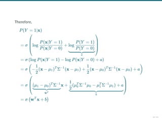
- 107. Using the Bayes' rule, we have: P(Y = 1∣x) = P(x) P(x∣Y = 1)P(Y = 1) = P(x∣Y = 0)P(Y = 0) + P(x∣Y = 1)P(Y = 1) P(x∣Y = 1)P(Y = 1) = . 1 + P(x∣Y =1)P(Y =1) P(x∣Y =0)P(Y =0) 1 15 / 61
- 108. Using the Bayes' rule, we have: It follows that with we get P(Y = 1∣x) = P(x) P(x∣Y = 1)P(Y = 1) = P(x∣Y = 0)P(Y = 0) + P(x∣Y = 1)P(Y = 1) P(x∣Y = 1)P(Y = 1) = . 1 + P(x∣Y =1)P(Y =1) P(x∣Y =0)P(Y =0) 1 σ(x) = , 1 + exp(−x) 1 P(Y = 1∣x) = σ log + log . ( P(x∣Y = 0) P(x∣Y = 1) P(Y = 0) P(Y = 1) ) 15 / 61
- 109. Therefore, P(Y = 1∣x) = σ log + ⎝ ⎜ ⎜ ⎛ P(x∣Y = 0) P(x∣Y = 1) a log P(Y = 0) P(Y = 1) ⎠ ⎟ ⎟ ⎞ = σ log P(x∣Y = 1) − log P(x∣Y = 0) + a ( ) = σ − (x − μ ) Σ (x − μ ) + (x − μ ) Σ (x − μ ) + a ( 2 1 1 T −1 1 2 1 0 T −1 0 ) = σ x + ⎝ ⎜ ⎛ wT (μ − μ ) Σ 1 0 T −1 b (μ Σ μ − μ Σ μ ) + a 2 1 0 T −1 0 1 T −1 1 ⎠ ⎟ ⎞ = σ w x + b ( T ) 16 / 61
- 110. 17 / 61
- 111. 17 / 61
- 112. 17 / 61
- 113. Note that the sigmoid function looks like a soft heavyside: Therefore, the overall model is very similar to the perceptron. σ(x) = 1 + exp(−x) 1 f(x; w, b) = σ(w x + b) T 18 / 61
- 114. x h w b dot add σ This unit is the lego brick of all neural networks! 19 / 61
- 115. Logistic regression Same model as for linear discriminant analysis. But, ignore model assumptions (Gaussian class populations, homoscedasticity); instead, nd that maximizes the likelihood of the data. P(Y = 1∣x) = σ w x + b ( T ) w, b 20 / 61
- 116. We have, This loss is an instance of the cross-entropy for and . arg P(d∣w, b) w,b max = arg P(Y = y ∣x , w, b) w,b max x ,y ∈d i i ∏ i i = arg σ(w x + b) (1 − σ(w x + b)) w,b max x ,y ∈d i i ∏ T i yi T i 1−yi = arg w,b min L(w,b)= ℓ(y , (x ;w,b)) ∑i i y ^ i −y log σ(w x + b) − (1 − y ) log(1 − σ(w x + b)) x ,y ∈d i i ∑ i T i i T i H(p, q) = E [− log q] p p = Y ∣xi q = ∣x Y ^ i 21 / 61
- 117. When takes values in , a similar derivation yields the logistic loss Y {−1, 1} L(w, b) = − log σ y (w x + b)) . x ,y ∈d i i ∑ ( i T i ) 22 / 61
- 118. In general, the cross-entropy and the logistic losses do not admit a minimizer that can be expressed analytically in closed form. However, a minimizer can be found numerically, using a general minimization technique such as gradient descent. 23 / 61
- 119. Gradient descent Let denote a loss function de ned over model parameters (e.g., and ). To minimize , gradient descent uses local linear information to iteratively move towards a (local) minimum. For , a rst-order approximation around can be de ned as L(θ) θ w b L(θ) θ ∈ R 0 d θ0 (θ + ϵ) = L(θ ) + ϵ ∇ L(θ ) + ∣∣ϵ∣∣ . L ^ 0 0 T θ 0 2γ 1 2 24 / 61
- 120. A minimizer of the approximation is given for which results in the best improvement for the step . Therefore, model parameters can be updated iteratively using the update rule where are the initial parameters of the model; is the learning rate; both are critical for the convergence of the update rule. (θ + ϵ) L ^ 0 ∇ (θ + ϵ) ϵL ^ 0 = 0 = ∇ L(θ ) + ϵ, θ 0 γ 1 ϵ = −γ∇ L(θ ) θ 0 θ = θ − γ∇ L(θ ), t+1 t θ t θ0 γ 25 / 61
- 121. Example 1: Convergence to a local minima 26 / 61
- 122. Example 1: Convergence to a local minima 26 / 61
- 123. Example 1: Convergence to a local minima 26 / 61
- 124. Example 1: Convergence to a local minima 26 / 61
- 125. Example 1: Convergence to a local minima 26 / 61
- 126. Example 1: Convergence to a local minima 26 / 61
- 127. Example 1: Convergence to a local minima 26 / 61
- 128. Example 1: Convergence to a local minima 26 / 61
- 129. Example 2: Convergence to the global minima 27 / 61
- 130. Example 2: Convergence to the global minima 27 / 61
- 131. Example 2: Convergence to the global minima 27 / 61
- 132. Example 2: Convergence to the global minima 27 / 61
- 133. Example 2: Convergence to the global minima 27 / 61
- 134. Example 2: Convergence to the global minima 27 / 61
- 135. Example 2: Convergence to the global minima 27 / 61
- 136. Example 2: Convergence to the global minima 27 / 61
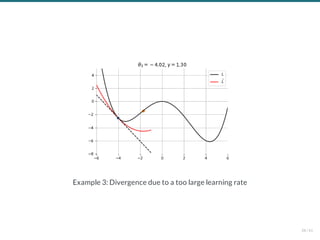
- 137. Example 3: Divergence due to a too large learning rate 28 / 61
- 138. Example 3: Divergence due to a too large learning rate 28 / 61
- 139. Example 3: Divergence due to a too large learning rate 28 / 61
- 140. Example 3: Divergence due to a too large learning rate 28 / 61
- 141. Example 3: Divergence due to a too large learning rate 28 / 61
- 142. Example 3: Divergence due to a too large learning rate 28 / 61
- 143. Stochastic gradient descent In the empirical risk minimization setup, and its gradient decompose as Therefore, in batch gradient descent the complexity of an update grows linearly with the size of the dataset. More importantly, since the empirical risk is already an approximation of the expected risk, it should not be necessary to carry out the minimization with great accuracy. L(θ) L(θ) ∇L(θ) = ℓ(y , f(x ; θ)) N 1 x ,y ∈d i i ∑ i i = ∇ℓ(y , f(x ; θ)). N 1 x ,y ∈d i i ∑ i i N 29 / 61
- 144. Instead, stochastic gradient descent uses as update rule: Iteration complexity is independent of . The stochastic process depends on the examples picked randomly at each iteration. θ = θ − γ∇ℓ(y , f(x ; θ )) t+1 t i(t+1) i(t+1) t N {θ ∣t = 1, ...} t i(t) 30 / 61
- 145. Batch gradient descent Stochastic gradient descent Instead, stochastic gradient descent uses as update rule: Iteration complexity is independent of . The stochastic process depends on the examples picked randomly at each iteration. θ = θ − γ∇ℓ(y , f(x ; θ )) t+1 t i(t+1) i(t+1) t N {θ ∣t = 1, ...} t i(t) 31 / 61
- 146. Why is stochastic gradient descent still a good idea? Informally, averaging the update over all choices restores batch gradient descent. Formally, if the gradient estimate is unbiased, e.g., if then the formal convergence of SGD can be proved, under appropriate assumptions (see references). Interestingly, if training examples are received and used in an online fashion, then SGD directly minimizes the expected risk. θ = θ − γ∇ℓ(y , f(x ; θ )) t+1 t i(t+1) i(t+1) t i(t + 1) E [∇ℓ(y , f(x ; θ ))] i(t+1) i(t+1) i(t+1) t = ∇ℓ(y , f(x ; θ )) N 1 x ,y ∈d i i ∑ i i t = ∇L(θ ) t x , y ∼ P i i X,Y 32 / 61
- 147. When decomposing the excess error in terms of approximation, estimation and optimization errors, stochastic algorithms yield the best generalization performance (in terms of expected risk) despite being the worst optimization algorithms (in terms of empirical risk) (Bottou, 2011). E R( ) − R(f ) [ f ~ ∗ d B ] = E R(f ) − R(f ) + E R(f ) − R(f ) + E R( ) − R(f ) [ ∗ B ] [ ∗ d ∗ ] [ f ~ ∗ d ∗ d ] = E + E + E app est opt 33 / 61
- 148. Layers So far we considered the logistic unit , where , , and . These units can be composed in parallel to form a layer with outputs: where , , , and where is upgraded to the element-wise sigmoid function. x h W b matmul add σ h = σ w x + b ( T ) h ∈ R x ∈ Rp w ∈ Rp b ∈ R q h = σ(W x + b) T h ∈ Rq x ∈ Rp W ∈ Rp×q b ∈ Rq σ(⋅) 34 / 61
- 149. Multi-layer perceptron Similarly, layers can be composed in series, such that: where denotes the model parameters . This model is the multi-layer perceptron, also known as the fully connected feedforward network. h0 h1 ... hL f(x; θ) = y ^ = x = σ(W h + b ) 1 T 0 1 = σ(W h + b ) L T L−1 L = hL θ {W , b , ...∣k = 1, ..., L} k k 35 / 61
- 150. x h1 W 1 b1 matmul add σ h2 W 2 b2 matmul add σ hL W L bL matmul add σ ... 36 / 61
- 151. Classi cation For binary classi cation, the width of the last layer is set to , which results in a single output that models the probability . For multi-class classi cation, the sigmoid action in the last layer can be generalized to produce a (normalized) vector of probability estimates . This activation is the function, where its -th output is de ned as for . q L 1 h ∈ [0, 1] L P(Y = 1∣x) σ h ∈ [0, 1] L C P(Y = i∣x) Softmax i Softmax(z) = , i exp(z ) ∑j=1 C j exp(z ) i i = 1, ..., C 37 / 61
- 152. Regression The last activation can be skipped to produce unbounded output values . σ h ∈ R L 38 / 61
- 153. Automatic differentiation To minimize with stochastic gradient descent, we need the gradient . Therefore, we require the evaluation of the (total) derivatives of the loss with respect to all model parameters , , for . These derivatives can be evaluated automatically from the computational graph of using automatic differentiation. L(θ) ∇ ℓ(θ ) θ t , dWk dℓ dbk dℓ ℓ Wk bk k = 1, ..., L ℓ 39 / 61
- 154. Chain rule g1 x g2 g3 ... gm f y u2 u3 u1 ... um Let us consider a 1-dimensional output composition , such that f ∘ g y u = f(u) = g(x) = (g (x), ..., g (x)). 1 m 40 / 61
- 155. The chain rule states that For the total derivative, the chain rule generalizes to (f ∘ g) = (f ∘ g)g . ′ ′ ′ dx dy = k=1 ∑ m ∂uk ∂y recursive case dx duk 41 / 61
- 156. Reverse automatic differentiation Since a neural network is a composition of differentiable functions, the total derivatives of the loss can be evaluated backward, by applying the chain rule recursively over its computational graph. The implementation of this procedure is called reverse automatic differentiation. 42 / 61
- 157. Let us consider a simpli ed 2-layer MLP and the following loss function: for , , and . f(x; W , W ) 1 2 ℓ(y, ; W , W ) y ^ 1 2 = σ W σ W x ( 2 T ( 1 T )) = cross_ent(y, ) + λ ∣∣W ∣∣ + ∣∣W ∣∣ y ^ ( 1 2 2 2) x ∈ Rp y ∈ R W ∈ R 1 p×q W ∈ R 2 q 43 / 61
- 158. In the forward pass, intermediate values are all computed from inputs to outputs, which results in the annotated computational graph below: x W 1 σ( ⋅ ) u1 u2 W 2 σ( ⋅ ) u3 ŷ y u4 || ⋅ ||2 u5 u6 u7 λ u8 l 44 / 61
- 159. The total derivative can be computed through a backward pass, by walking through all paths from outputs to parameters in the computational graph and accumulating the terms. For example, for we have: x W 1 σ( ⋅ ) u1 u2 W 2 σ( ⋅ ) u3 ŷ y u4 || ⋅ ||2 u5 u6 u7 λ u8 l dW1 dℓ dW1 dℓ dW1 du8 = + ∂u8 ∂ℓ dW1 du8 ∂u4 ∂ℓ dW1 du4 = ... 45 / 61
- 160. x W 1 σ( ⋅ ) u1 u2 W 2 σ( ⋅ ) u3 ŷ Let us zoom in on the computation of the network output and of its derivative with respect to . Forward pass: values , , and are computed by traversing the graph from inputs to outputs given , and . Backward pass: by the chain rule we have Note how evaluating the partial derivatives requires the intermediate values computed forward. y ^ W1 u1 u2 u3 y ^ x W1 W2 dW1 dy ^ = ∂u3 ∂y ^ ∂u2 ∂u3 ∂u1 ∂u2 ∂W1 ∂u1 = ∂u3 ∂σ(u ) 3 ∂u2 ∂W u 2 T 2 ∂u1 ∂σ(u ) 1 ∂W1 ∂W u 1 T 1 46 / 61
- 161. This algorithm is also known as backpropagation. An equivalent procedure can be de ned to evaluate the derivatives in forward mode, from inputs to outputs. Since differentiation is a linear operator, automatic differentiation can be implemented ef ciently in terms of tensor operations. 47 / 61
- 162. Vanishing gradients Training deep MLPs with many layers has for long (pre-2011) been very dif cult due to the vanishing gradient problem. Small gradients slow down, and eventually block, stochastic gradient descent. This results in a limited capacity of learning. Backpropagated gradients normalized histograms (Glorot and Bengio,2010). Gradients for layers far fromthe output vanish to zero. 48 / 61
- 163. Let us consider a simpli ed 3-layer MLP, with , such that Under the hood, this would be evaluated as and its derivative as x, w , w , w ∈ R 1 2 3 f(x; w , w , w ) = σ w σ w σ w x . 1 2 3 ( 3 ( 2 ( 1 ))) u1 u2 u3 u4 u5 y ^ = w x 1 = σ(u ) 1 = w u 2 2 = σ(u ) 3 = w u 3 4 = σ(u ) 5 dw1 dy ^ dw1 dy ^ = ∂u5 ∂y ^ ∂u4 ∂u5 ∂u3 ∂u4 ∂u2 ∂u3 ∂u1 ∂u2 ∂w1 ∂u1 = w w x ∂u5 ∂σ(u ) 5 3 ∂u3 ∂σ(u ) 3 2 ∂u1 ∂σ(u ) 1 49 / 61
- 164. The derivative of the sigmoid activation function is: Notice that for all . σ (x) = σ(x)(1 − σ(x)) dx dσ 0 ≤ (x) ≤ dx dσ 4 1 x 50 / 61
- 165. Assume that weights are initialized randomly from a Gaussian with zero-mean and small variance, such that with high probability . Then, This implies that the gradient exponentially shrinks to zero as the number of layers in the network increases. Hence the vanishing gradient problem. In general, bounded activation functions (sigmoid, tanh, etc) are prone to the vanishing gradient problem. Note the importance of a proper initialization scheme. w , w , w 1 2 3 −1 ≤ w ≤ 1 i = x dw1 dy ^ ≤4 1 ∂u5 ∂σ(u ) 5 ≤1 w3 ≤4 1 ∂u3 ∂σ(u ) 3 ≤1 w2 ≤4 1 ∂u1 σ(u ) 1 dw1 dy ^ 51 / 61
- 166. Recti ed linear units Instead of the sigmoid activation function, modern neural networks are for most based on recti ed linear units (ReLU) (Glorot et al, 2011): ReLU(x) = max(0, x) 52 / 61
- 167. Note that the derivative of the ReLU function is For , the derivative is unde ned. In practice, it is set to zero. ReLU(x) = dx d { 0 1 if x ≤ 0 otherwise x = 0 53 / 61
- 168. Therefore, This solves the vanishing gradient problem, even for deep networks! (provided proper initialization) Note that: The ReLU unit dies when its input is negative, which might block gradient descent. This is actually a useful property to induce sparsity. This issue can also be solved using leaky ReLUs, de ned as for a small (e.g., ). = w w x dw1 dy ^ =1 ∂u5 ∂σ(u ) 5 3 =1 ∂u3 ∂σ(u ) 3 2 =1 ∂u1 ∂σ(u ) 1 LeakyReLU(x) = max(αx, x) α ∈ R+ α = 0.1 54 / 61
- 169. Universal approximation Theorem. (Cybenko 1989; Hornik et al, 1991) Let be a bounded, non- constant continuous function. Let denote the -dimensional hypercube, and denote the space of continuous functions on . Given any and , there exists and such that satis es It guarantees that even a single hidden-layer network can represent any classi cation problem in which the boundary is locally linear (smooth); It does not inform about good/bad architectures, nor how they relate to the optimization procedure. The universal approximation theorem generalizes to any non-polynomial (possibly unbounded) activation function, including the ReLU (Leshno, 1993). σ(⋅) Ip p C(I ) p Ip f ∈ C(I ) p ϵ > 0 q > 0 v , w , b , i = 1, ..., q i i i F(x) = v σ(w x + b ) i≤q ∑ i i T i ∣f(x) − F(x)∣ < ϵ. x∈Ip sup 55 / 61
- 170. Theorem (Barron, 1992) The mean integrated square error between the estimated network and the target function is bounded by where is the number of training points, is the number of neurons, is the input dimension, and measures the global smoothness of . Combines approximation and estimation errors. Provided enough data, it guarantees that adding more neurons will result in a better approximation. F ^ f O + log N ( q Cf 2 N qp ) N q p Cf f 56 / 61
- 171. Let us consider the 1-layer MLP This model can approximate any smooth 1D function, provided enough hidden units. f(x) = w ReLU(x + b ). ∑ i i 57 / 61
- 172. Let us consider the 1-layer MLP This model can approximate any smooth 1D function, provided enough hidden units. f(x) = w ReLU(x + b ). ∑ i i 57 / 61
- 173. Let us consider the 1-layer MLP This model can approximate any smooth 1D function, provided enough hidden units. f(x) = w ReLU(x + b ). ∑ i i 57 / 61
- 174. Let us consider the 1-layer MLP This model can approximate any smooth 1D function, provided enough hidden units. f(x) = w ReLU(x + b ). ∑ i i 57 / 61
- 175. Let us consider the 1-layer MLP This model can approximate any smooth 1D function, provided enough hidden units. f(x) = w ReLU(x + b ). ∑ i i 57 / 61
- 176. Let us consider the 1-layer MLP This model can approximate any smooth 1D function, provided enough hidden units. f(x) = w ReLU(x + b ). ∑ i i 57 / 61
- 177. Let us consider the 1-layer MLP This model can approximate any smooth 1D function, provided enough hidden units. f(x) = w ReLU(x + b ). ∑ i i 57 / 61
- 178. Let us consider the 1-layer MLP This model can approximate any smooth 1D function, provided enough hidden units. f(x) = w ReLU(x + b ). ∑ i i 57 / 61
- 179. Let us consider the 1-layer MLP This model can approximate any smooth 1D function, provided enough hidden units. f(x) = w ReLU(x + b ). ∑ i i 57 / 61
- 180. Let us consider the 1-layer MLP This model can approximate any smooth 1D function, provided enough hidden units. f(x) = w ReLU(x + b ). ∑ i i 57 / 61
- 181. Let us consider the 1-layer MLP This model can approximate any smooth 1D function, provided enough hidden units. f(x) = w ReLU(x + b ). ∑ i i 57 / 61
- 182. Let us consider the 1-layer MLP This model can approximate any smooth 1D function, provided enough hidden units. f(x) = w ReLU(x + b ). ∑ i i 57 / 61
- 183. Let us consider the 1-layer MLP This model can approximate any smooth 1D function, provided enough hidden units. f(x) = w ReLU(x + b ). ∑ i i 57 / 61
- 184. Effect of depth Theorem (Montúfar et al, 2014) A recti er neural network with input units and hidden layers of width can compute functions that have linear regions. That is, the number of linear regions of deep models grows exponentially in and polynomially in . Even for small values of and , deep recti er models are able to produce substantially more linear regions than shallow recti er models. p L q ≥ p Ω(( ) q ) p q (L−1)p p L q L q 58 / 61
- 185. Deep learning Recent advances and model architectures in deep learning are built on a natural generalization of a neural network: a graph of tensor operators, taking advantage of the chain rule stochastic gradient descent convolutions parallel operations on GPUs. This does not differ much from networks from the 90s, as covered in Today's lecture. ――― Credits: Francois Fleuret, EE559 Deep Learning, EPFL. 59 / 61
- 186. This generalization allows to compose and design complex networks of operators, possibly dynamically, dealing with images, sound, text, sequences, etc. and to train them end-to-end. ――― Credits: Francois Fleuret, EE559 Deep Learning, EPFL; Rahmatizadeh et al, 2017, arXiv:1707.02920. 60 / 61
- 187. The end. 60 / 61
- 188. References Rosenblatt, F. (1958). The perceptron: a probabilistic model for information storage and organization in the brain. Psychological review, 65(6), 386. Bottou, L., & Bousquet, O. (2008). The tradeoffs of large scale learning. In Advances in neural information processing systems (pp. 161-168). Rumelhart, D. E., Hinton, G. E., & Williams, R. J. (1986). Learning representations by back-propagating errors. nature, 323(6088), 533. Cybenko, G. (1989). Approximation by superpositions of a sigmoidal function. Mathematics of control, signals and systems, 2(4), 303-314. Montufar, G. F., Pascanu, R., Cho, K., & Bengio, Y. (2014). On the number of linear regions of deep neural networks. In Advances in neural information processing systems (pp. 2924-2932). 61 / 61
- 189. Deep Learning Lecture 3: Convolutional networks Prof. Gilles Louppe g.louppe@uliege.be 1 / 71
- 190. Today How to make neural networks see? A little history Convolutions Convolutional network architectures What is really happening? 2 / 71
- 191. A little history Adapted from Yannis Avrithis, "Lecture 1: Introduction", Deep Learning for vision, 2018. 3 / 71
- 192. Visual perception (Hubel and Wiesel, 1959-1962) David Hubel and Torsten Wiesel discover the neural basis of visual perception. Nobel Prize of Medicine in 1981 for this work. 4 / 71
- 193. Hubel & Wiesel 1: Intro Hubel & Wiesel 1: Intro Hubel & Wiesel 1: Intro Watch later Share Hubel and Wiesel 5 / 71
- 194. ――― Credits: Hubel and Wiesel, Receptive elds, binocular interaction and functional architecture in the cat's visual cortex, 1962. 6 / 71
- 195. ――― Credits: Hubel and Wiesel, Receptive elds, binocular interaction and functional architecture in the cat's visual cortex, 1962. 7 / 71
- 196. Perceptron (Rosenblatt, 1959) The Mark-1 Perceptron: Analog circuit implementation of a neural network, Parameters as potentiometers. ――― Credits: Frank Rosenblatt, Principle of Neurodynamics, 1961. 8 / 71
- 197. "If we show the perceptron a stimulus, say a square, and associate a response to that square, this response will immediately generalize perfectly to all transforms of the square under the transformation group [...]." This is quite similar to Hubel and Wiesel's simple and complex cells! ――― Credits: Frank Rosenblatt, Principle of Neurodynamics, 1961. 9 / 71
- 198. AI winter (Minsky and Papert, 1969+) Minsky and Papert rede ne the perceptron as a linear classi er, Then they prove a series of impossiblity results. AI winter follows. ――― Credits: Minsky and Papert, Perceptrons: an Introduction to Computational Geometry, 1969. 10 / 71
- 199. Automatic differentiation (Werbos, 1974) Formulate an arbitrary function as computational graph. Dynamic feedback: compute symbolic derivatives by dynamic programming. ――― Credits: Paul Werbos, Beyond regression: new tools for prediction and analysis in the behavioral sciences, 1974. 11 / 71
- 200. Neocognitron (Fukushima, 1980) Fukushima proposes a direct neural network implementation of the hierarchy model of the visual nervous system of Hubel and Wiesel. ――― Credits: Kunihiko Fukushima, Neocognitron: A Self-organizing Neural Network Model, 1980. 12 / 71
- 201. Convolutions Feature hierarchy Built upon convolutions and enables the composition of a feature hierarchy. Biologically-inspired training algorithm, which proves to be largely inef cient. ――― Credits: Kunihiko Fukushima, Neocognitron: A Self-organizing Neural Network Model, 1980. 13 / 71
- 202. Introduce backpropagation in multi-layer networks with sigmoid non-linearities and sum of squares loss function. Advocate batch gradient descent for supervised learning. Discuss online gradient descent, momentum and random initialization. Depart from biologically plausible training algorithms. Backpropagation (Rumelhart et al, 1986) ――― Credits: Rumelhart et al, Learning representations by back-propagating errors, 1986. 14 / 71
- 203. Convolutional networks (LeCun, 1990) Train a convolutional network by backpropagation. Advocate end-to-end feature learning for image classi cation. ――― Credits: LeCun et al, Handwritten Digit Recognition with a Back-Propagation Network, 1990. 15 / 71
- 204. Convolutional Network Demo from 1993 Convolutional Network Demo from 1993 Convolutional Network Demo from 1993 Watch later Share LeNet-1 (LeCun et al, 1993) 16 / 71
- 205. Object detection (Redmon et al, 2015) Geometric matching (Rocco et al, 2017) Semantic segmentation (Long et al, 2015) Instance segmentation (He et al, 2017) Convolutional networks are now used everywhere in vision. 17 / 71
- 206. ... but also in many other applications, including: speech recognition and synthesis natural language processing protein/DNA binding prediction or more generally, any problem with a spatial (or sequential) structure. 18 / 71
- 207. Convolutions 19 / 71
- 208. Let us consider the rst layer of a MLP taking images as input. What are the problems with this architecture? ――― Credits: Yannis Avrithis, Deep Learning for Vision, University of Rennes 1. 20 / 71
- 209. Issues Too many parameters: . What if images are ? What if the rst layercounts units? Spatial organization of the input is destroyed. The network is not invariant to transformations (e.g., translation). 100 × 784 + 100 640 × 480 × 3 1000 21 / 71
- 210. Instead, let us only keep a sparse set of connections, where all weights having the same color are shared. ――― Credits: Yannis Avrithis, Deep Learning for Vision, University of Rennes 1. 22 / 71
- 211. The resulting operation can be seen as shifting the same weight triplet (kernel). The set of inputs seen by each unit is its receptive eld. This is a 1D convolution, which can be generalized to more dimensions. ⇒ 23 / 71
- 212. Convolutions For one-dimensional tensors, given an input vector and a convolutional kernel , the discrete convolution is a vector of size such that Technically, denotes the cross-correlation operator. However, most machine learning libraries call it convolution. x ∈ RW u ∈ Rw u ⋆ x W − w + 1 (u ⋆ x)[i] = u x . m=0 ∑ w−1 m m+i ⋆ 24 / 71
- 213. ――― Credits: Francois Fleuret, EE559 Deep Learning, EPFL. 25 / 71
- 214. Convolutions generalize to multi-dimensional tensors: In its most usual form, a convolution takes as input a 3D tensor , called the input feature map. A kernel slides across the input feature map, along its height and width. The size is the size of the receptive eld. At each location, the element-wise product between the kernel and the input elements it overlaps is computed and the results are summed up. x ∈ RC×H×W u ∈ RC×h×w h × w 26 / 71
- 215. ――― Credits: Francois Fleuret, EE559 Deep Learning, EPFL. 27 / 71
- 216. The nal output is a 2D tensor of size called the output feature map and such that: where and are shared parameters to learn. convolutions can be applied in the same way to produce a feature map, where is the depth. o (H − h + 1) × (W − w + 1) oj,i = b + (u ⋆ x )[j, i] = b + u x j,i c=0 ∑ C−1 c c j,i c=0 ∑ C−1 n=0 ∑ h−1 m=0 ∑ w−1 c,n,m c,n+j,m+i u b D D × (H − h + 1) × (W − w + 1) D 28 / 71
- 217. Convolution as a matrix multiplication As a guiding example, let us consider the convolution of single-channel tensors and : x ∈ R4×4 u ∈ R3×3 u ⋆ x = ⋆ = ⎝ ⎛1 1 3 4 4 3 1 3 1⎠ ⎞ ⎝ ⎜ ⎜ ⎛4 1 3 6 5 8 6 5 8 8 6 7 7 8 4 8⎠ ⎟ ⎟ ⎞ ( 122 126 148 134 ) 29 / 71
- 218. The convolution operation can be equivalently re-expressed as a single matrix multiplication: the convolutional kernel is rearranged as a sparse Toeplitz circulant matrix, called the convolution matrix: the input is attened row by row, from top to bottom: Then, which we can reshape to a matrix to obtain . u U = ⎝ ⎜ ⎜ ⎛1 0 0 0 4 1 0 0 1 4 0 0 0 1 0 0 1 0 1 0 4 1 4 1 3 4 1 4 0 3 0 1 3 0 1 0 3 3 4 1 1 3 3 4 0 1 0 3 0 0 3 0 0 0 3 3 0 0 1 3 0 0 0 1⎠ ⎟ ⎟ ⎞ x v(x) = (4 5 8 7 1 8 8 8 3 6 6 4 6 5 7 8) T Uv(x) = (122 148 126 134) T 2 × 2 u ⋆ x 30 / 71
- 219. The same procedure generalizes to and convolutional kernel , such that: the convolutional kernel is rearranged as a sparse Toeplitz circulant matrix of shape where each row identi es an element of theoutput featuremap, each column identi es an element of theinput featuremap, thevalue corresponds to thekernel valuetheelement is multiplied with in output ; the input is attened into a column vector of shape ; the output feature map is obtained by reshaping the column vector as a matrix. Therefore, a convolutional layer is a special case of a fully connected layer: x ∈ RH×W u ∈ Rh×w U (H − h + 1)(W − w + 1) × HW i j Ui,j j i x v(x) HW × 1 u ⋆ x (H − h + 1)(W − w + 1) × 1 Uv(x) (H − h + 1) × (W − w + 1) h = u ⋆ x ⇔ v(h) = Uv(x) ⇔ v(h) = W v(x) T 31 / 71
- 220. x h u ⋆ x h U flatten matmul reshape ⇔ 32 / 71
- 221. Strides The stride speci es the size of the step for the convolution operator. This parameter reduces the size of the output map. ――― Credits: Dumoulin and Visin, A guide to convolution arithmetic for deep learning, 2016. 33 / 71
- 222. Padding Padding speci es whether the input volume is padded arti cially around its border. This parameter is useful to keep spatial dimensions constant across lters. Zero-padding is the default mode. ――― Credits: Dumoulin and Visin, A guide to convolution arithmetic for deep learning, 2016. 34 / 71
- 223. Equivariance A function is equivariant to if . Parameter sharing used in a convolutional layer causes the layer to be equivariant to translation. That is, if is any function that translates the input, the convolution function is equivariant to . If an object moves in the input image,its representation will move the same amount in the output. f g f(g(x)) = g(f(x)) g g ――― Credits: LeCun et al, Gradient-based learning applied to document recognition, 1998. 35 / 71
- 224. Equivariance is useful when we know some local function is useful everywhere (e.g., edge detectors). Convolution is not equivariant to other operations such as change in scale or rotation. 36 / 71
- 225. Pooling When the input volume is large, pooling layers can be used to reduce the input dimension while preserving its global structure, in a way similar to a down-scaling operation. Consider a pooling area of size and a 3D input tensor . Max-pooling produces a tensor such that Average pooling produces a tensor such that Pooling is very similar in its formulation to convolution. h × w x ∈ RC×(rh)×(sw) o ∈ RC×r×s o = x . c,j,i n<h,m<w max c,rj+n,si+m o ∈ RC×r×s o = x . c,j,i hw 1 n=0 ∑ h−1 m=0 ∑ w−1 c,rj+n,si+m 37 / 71
- 226. ――― Credits: Francois Fleuret, EE559 Deep Learning, EPFL. 38 / 71
- 227. Invariance A function is invariant to if . Pooling layers can be used for building inner activations that are (slightly) invariant to small translations of the input. Invariance to local translation is helpful if we care more about the presence of a pattern rather than its exact position. f g f(g(x)) = f(x) 39 / 71
- 229. Layer patterns A convolutional network can often be de ned as a composition of convolutional layers ( ), pooling layers ( ), linear recti ers ( ) and fully connected layers ( ). CONV POOL RELU FC 41 / 71
- 230. The most common convolutional network architecture follows the pattern: where: indicates repetition; indicates an optional pooling layer; (and usually ), , (and usually ); the last fully connected layer holds the output (e.g., the class scores). INPUT → [[CONV → RELU]*N → POOL?]*M → [FC → RELU]*K → FC * POOL? N ≥ 0 N ≤ 3 M ≥ 0 K ≥ 0 K < 3 42 / 71
- 231. Architectures Some common architectures for convolutional networks following this pattern include: , which implements a linear classi er ( ). , which implements a -layer MLP. . . . INPUT → FC N = M = K = 0 INPUT → [FC → RELU]∗K → FC K INPUT → CONV → RELU → FC INPUT → [CONV → RELU → POOL]*2 → FC → RELU → FC INPUT → [[CONV → RELU]*2 → POOL]*3 → [FC → RELU]*2 → FC 43 / 71
- 232. 44 / 71
- 233. LeNet-5 (LeCun et al, 1998) First convolutional network to use backpropagation. Applied to character recognition. 45 / 71
- 234. ---------------------------------------------------------------- Layer (type) Output Shape Param # ================================================================ Conv2d-1 [-1, 6, 28, 28] 156 ReLU-2 [-1, 6, 28, 28] 0 MaxPool2d-3 [-1, 6, 14, 14] 0 Conv2d-4 [-1, 16, 10, 10] 2,416 ReLU-5 [-1, 16, 10, 10] 0 MaxPool2d-6 [-1, 16, 5, 5] 0 Conv2d-7 [-1, 120, 1, 1] 48,120 ReLU-8 [-1, 120, 1, 1] 0 Linear-9 [-1, 84] 10,164 ReLU-10 [-1, 84] 0 Linear-11 [-1, 10] 850 LogSoftmax-12 [-1, 10] 0 ================================================================ Total params: 61,706 Trainable params: 61,706 Non-trainable params: 0 ---------------------------------------------------------------- Input size (MB): 0.00 Forward/backward pass size (MB): 0.11 Params size (MB): 0.24 Estimated Total Size (MB): 0.35 ---------------------------------------------------------------- 46 / 71
- 235. AlexNet (Krizhevsky et al, 2012) 16.4% top-5 error on ILSVRC'12, outperformed all by 10%. Implementation on two GPUs, because of memory constraints. 47 / 71
- 236. ---------------------------------------------------------------- Layer (type) Output Shape Param # ================================================================ Conv2d-1 [-1, 64, 55, 55] 23,296 ReLU-2 [-1, 64, 55, 55] 0 MaxPool2d-3 [-1, 64, 27, 27] 0 Conv2d-4 [-1, 192, 27, 27] 307,392 ReLU-5 [-1, 192, 27, 27] 0 MaxPool2d-6 [-1, 192, 13, 13] 0 Conv2d-7 [-1, 384, 13, 13] 663,936 ReLU-8 [-1, 384, 13, 13] 0 Conv2d-9 [-1, 256, 13, 13] 884,992 ReLU-10 [-1, 256, 13, 13] 0 Conv2d-11 [-1, 256, 13, 13] 590,080 ReLU-12 [-1, 256, 13, 13] 0 MaxPool2d-13 [-1, 256, 6, 6] 0 Dropout-14 [-1, 9216] 0 Linear-15 [-1, 4096] 37,752,832 ReLU-16 [-1, 4096] 0 Dropout-17 [-1, 4096] 0 Linear-18 [-1, 4096] 16,781,312 ReLU-19 [-1, 4096] 0 Linear-20 [-1, 1000] 4,097,000 ================================================================ Total params: 61,100,840 Trainable params: 61,100,840 Non-trainable params: 0 ---------------------------------------------------------------- Input size (MB): 0.57 Forward/backward pass size (MB): 8.31 Params size (MB): 233.08 Estimated Total Size (MB): 241.96 ---------------------------------------------------------------- 48 / 71
- 237. 96 kernels learned by the rst convolutional layer. Top 48 kernels were learned on GPU1, while the bottom 48 kernels were learned on GPU 2. 11 × 11 × 3 49 / 71
- 238. VGG (Simonyan and Zisserman, 2014) 7.3% top-5 error on ILSVRC'14. Depth increased up to 19 layers, kernel sizes reduced to 3. 50 / 71
- 239. ---------------------------------------------------------------- Layer (type) Output Shape Param # ================================================================ Conv2d-1 [-1, 64, 224, 224] 1,792 ReLU-2 [-1, 64, 224, 224] 0 Conv2d-3 [-1, 64, 224, 224] 36,928 ReLU-4 [-1, 64, 224, 224] 0 MaxPool2d-5 [-1, 64, 112, 112] 0 Conv2d-6 [-1, 128, 112, 112] 73,856 ReLU-7 [-1, 128, 112, 112] 0 Conv2d-8 [-1, 128, 112, 112] 147,584 ReLU-9 [-1, 128, 112, 112] 0 MaxPool2d-10 [-1, 128, 56, 56] 0 Conv2d-11 [-1, 256, 56, 56] 295,168 ReLU-12 [-1, 256, 56, 56] 0 Conv2d-13 [-1, 256, 56, 56] 590,080 ReLU-14 [-1, 256, 56, 56] 0 Conv2d-15 [-1, 256, 56, 56] 590,080 ReLU-16 [-1, 256, 56, 56] 0 MaxPool2d-17 [-1, 256, 28, 28] 0 Conv2d-18 [-1, 512, 28, 28] 1,180,160 ReLU-19 [-1, 512, 28, 28] 0 Conv2d-20 [-1, 512, 28, 28] 2,359,808 ReLU-21 [-1, 512, 28, 28] 0 Conv2d-22 [-1, 512, 28, 28] 2,359,808 ReLU-23 [-1, 512, 28, 28] 0 MaxPool2d-24 [-1, 512, 14, 14] 0 Conv2d-25 [-1, 512, 14, 14] 2,359,808 ReLU-26 [-1, 512, 14, 14] 0 Conv2d-27 [-1, 512, 14, 14] 2,359,808 ReLU-28 [-1, 512, 14, 14] 0 Conv2d-29 [-1, 512, 14, 14] 2,359,808 ReLU-30 [-1, 512, 14, 14] 0 MaxPool2d-31 [-1, 512, 7, 7] 0 Linear-32 [-1, 4096] 102,764,544 ReLU-33 [-1, 4096] 0 Dropout-34 [-1, 4096] 0 Linear-35 [-1, 4096] 16,781,312 ReLU-36 [-1, 4096] 0 Dropout-37 [-1, 4096] 0 Linear-38 [-1, 1000] 4,097,000 ================================================================ Total params: 138,357,544 Trainable params: 138,357,544 Non-trainable params: 0 ---------------------------------------------------------------- Input size (MB): 0.57 Forward/backward pass size (MB): 218.59 Params size (MB): 527.79 Estimated Total Size (MB): 746.96 ---------------------------------------------------------------- 51 / 71
- 240. The effective receptive eld is the part of the visual input that affects a given unit indirectly through previous layers. It grows linearly with depth. A stack of three kernels of stride 1 has the same effective receptive eld as a single kernel, but fewer parameters. 3 × 3 7 × 7 ――― Credits: Yannis Avrithis, Deep Learning for Vision, University of Rennes 1. 52 / 71
- 241. ResNet (He et al, 2015) Even deeper models (34, 50, 101 and 152 layers) Skip connections. Resnet-50 vs. VGG: 5.25% top-5 errorvs. 7.1% 25M vs. 138M parameters 3.8BFlops vs. 15.3BFlops Fully convolutional until thelast layer 53 / 71
- 242. ---------------------------------------------------------------- Layer (type) Output Shape Param # ================================================================ Conv2d-1 [-1, 64, 112, 112] 9,408 BatchNorm2d-2 [-1, 64, 112, 112] 128 ReLU-3 [-1, 64, 112, 112] 0 MaxPool2d-4 [-1, 64, 56, 56] 0 Conv2d-5 [-1, 64, 56, 56] 4,096 BatchNorm2d-6 [-1, 64, 56, 56] 128 ReLU-7 [-1, 64, 56, 56] 0 Conv2d-8 [-1, 64, 56, 56] 36,864 BatchNorm2d-9 [-1, 64, 56, 56] 128 ReLU-10 [-1, 64, 56, 56] 0 Conv2d-11 [-1, 256, 56, 56] 16,384 BatchNorm2d-12 [-1, 256, 56, 56] 512 Conv2d-13 [-1, 256, 56, 56] 16,384 BatchNorm2d-14 [-1, 256, 56, 56] 512 ReLU-15 [-1, 256, 56, 56] 0 Bottleneck-16 [-1, 256, 56, 56] 0 Conv2d-17 [-1, 64, 56, 56] 16,384 BatchNorm2d-18 [-1, 64, 56, 56] 128 ReLU-19 [-1, 64, 56, 56] 0 Conv2d-20 [-1, 64, 56, 56] 36,864 BatchNorm2d-21 [-1, 64, 56, 56] 128 ReLU-22 [-1, 64, 56, 56] 0 Conv2d-23 [-1, 256, 56, 56] 16,384 BatchNorm2d-24 [-1, 256, 56, 56] 512 ReLU-25 [-1, 256, 56, 56] 0 Bottleneck-26 [-1, 256, 56, 56] 0 Conv2d-27 [-1, 64, 56, 56] 16,384 BatchNorm2d-28 [-1, 64, 56, 56] 128 ReLU-29 [-1, 64, 56, 56] 0 Conv2d-30 [-1, 64, 56, 56] 36,864 BatchNorm2d-31 [-1, 64, 56, 56] 128 ReLU-32 [-1, 64, 56, 56] 0 Conv2d-33 [-1, 256, 56, 56] 16,384 BatchNorm2d-34 [-1, 256, 56, 56] 512 ReLU-35 [-1, 256, 56, 56] 0 Bottleneck-36 [-1, 256, 56, 56] 0 Conv2d-37 [-1, 128, 56, 56] 32,768 BatchNorm2d-38 [-1, 128, 56, 56] 256 ReLU-39 [-1, 128, 56, 56] 0 Conv2d-40 [-1, 128, 28, 28] 147,456 BatchNorm2d-41 [-1, 128, 28, 28] 256 ReLU-42 [-1, 128, 28, 28] 0 Conv2d-43 [-1, 512, 28, 28] 65,536 BatchNorm2d-44 [-1, 512, 28, 28] 1,024 Conv2d-45 [-1, 512, 28, 28] 131,072 BatchNorm2d-46 [-1, 512, 28, 28] 1,024 ReLU-47 [-1, 512, 28, 28] 0 Bottleneck-48 [-1, 512, 28, 28] 0 Conv2d-49 [-1, 128, 28, 28] 65,536 BatchNorm2d-50 [-1, 128, 28, 28] 256 ReLU-51 [-1, 128, 28, 28] 0 Conv2d-52 [-1, 128, 28, 28] 147,456 BatchNorm2d-53 [-1, 128, 28, 28] 256 ... ... Bottleneck-130 [-1, 1024, 14, 14] 0 Conv2d-131 [-1, 256, 14, 14] 262,144 BatchNorm2d-132 [-1, 256, 14, 14] 512 ReLU-133 [-1, 256, 14, 14] 0 Conv2d-134 [-1, 256, 14, 14] 589,824 BatchNorm2d-135 [-1, 256, 14, 14] 512 ReLU-136 [-1, 256, 14, 14] 0 Conv2d-137 [-1, 1024, 14, 14] 262,144 BatchNorm2d-138 [-1, 1024, 14, 14] 2,048 ReLU-139 [-1, 1024, 14, 14] 0 Bottleneck-140 [-1, 1024, 14, 14] 0 Conv2d-141 [-1, 512, 14, 14] 524,288 BatchNorm2d-142 [-1, 512, 14, 14] 1,024 ReLU-143 [-1, 512, 14, 14] 0 Conv2d-144 [-1, 512, 7, 7] 2,359,296 BatchNorm2d-145 [-1, 512, 7, 7] 1,024 ReLU-146 [-1, 512, 7, 7] 0 Conv2d-147 [-1, 2048, 7, 7] 1,048,576 BatchNorm2d-148 [-1, 2048, 7, 7] 4,096 Conv2d-149 [-1, 2048, 7, 7] 2,097,152 BatchNorm2d-150 [-1, 2048, 7, 7] 4,096 ReLU-151 [-1, 2048, 7, 7] 0 Bottleneck-152 [-1, 2048, 7, 7] 0 Conv2d-153 [-1, 512, 7, 7] 1,048,576 BatchNorm2d-154 [-1, 512, 7, 7] 1,024 ReLU-155 [-1, 512, 7, 7] 0 Conv2d-156 [-1, 512, 7, 7] 2,359,296 BatchNorm2d-157 [-1, 512, 7, 7] 1,024 ReLU-158 [-1, 512, 7, 7] 0 Conv2d-159 [-1, 2048, 7, 7] 1,048,576 BatchNorm2d-160 [-1, 2048, 7, 7] 4,096 ReLU-161 [-1, 2048, 7, 7] 0 Bottleneck-162 [-1, 2048, 7, 7] 0 Conv2d-163 [-1, 512, 7, 7] 1,048,576 BatchNorm2d-164 [-1, 512, 7, 7] 1,024 ReLU-165 [-1, 512, 7, 7] 0 Conv2d-166 [-1, 512, 7, 7] 2,359,296 BatchNorm2d-167 [-1, 512, 7, 7] 1,024 ReLU-168 [-1, 512, 7, 7] 0 Conv2d-169 [-1, 2048, 7, 7] 1,048,576 BatchNorm2d-170 [-1, 2048, 7, 7] 4,096 ReLU-171 [-1, 2048, 7, 7] 0 Bottleneck-172 [-1, 2048, 7, 7] 0 AvgPool2d-173 [-1, 2048, 1, 1] 0 Linear-174 [-1, 1000] 2,049,000 ================================================================ Total params: 25,557,032 Trainable params: 25,557,032 Non-trainable params: 0 ---------------------------------------------------------------- Input size (MB): 0.57 Forward/backward pass size (MB): 286.56 Params size (MB): 97.49 Estimated Total Size (MB): 384.62 ---------------------------------------------------------------- 54 / 71
- 243. Deeper is better 55 / 71
- 244. Finding the optimal neural network architecture remains an active area of research. ――― Credits: Canziani et al, An Analysis of Deep Neural Network Models for Practical Applications, 2016. 56 / 71
- 245. Pre-trained models Training a model on natural images, from scratch, takes days or weeks. Many models trained on ImageNet are publicly available for download. These models can be used as feature extractors or for smart initialization. 57 / 71
- 246. Transfer learning Take a pre-trained network, remove the last layer(s) and then treat the rest of the the network as a xed feature extractor. Train a model from these features on a new task. Often better than handcrafted feature extraction for natural images, or better than training from data of the new task only. Fine tuning Same as for transfer learning, but also ne-tune the weights of the pre- trained network by continuing backpropagation. All or only some of the layers can be tuned. 58 / 71
- 247. In the case of models pre-trained on ImageNet, this often works even when input images for the new task are not photographs of objects or animals, such as biomedical images, satellite images or paintings. ――― Credits: Mormont et al, Comparison of deep transfer learning strategies for digital pathology, 2018. 59 / 71
- 248. What is really happening? 60 / 71
- 249. Maximum response samples Convolutional networks can be inspected by looking for input images that maximize the activation of a chosen convolutional kernel at layer and index in the layer lter bank. Such images can be found by gradient ascent on the input space: x h (x) ℓ,d u ℓ d L (x) ℓ,d x0 xt+1 = ∣∣h (x)∣∣ ℓ,d 2 ∼ U[0, 1]C×H×W = x + γ∇ L (x ) t x ℓ,d t 61 / 71
- 250. VGG-16, convolutional layer 1-1, a few of the 64 lters ――― Credits: Francois Chollet, How convolutional neural networks see the world, 2016. 62 / 71
- 251. VGG-16, convolutional layer 2-1, a few of the 128 lters ――― Credits: Francois Chollet, How convolutional neural networks see the world, 2016. 63 / 71
- 252. VGG-16, convolutional layer 3-1, a few of the 256 lters ――― Credits: Francois Chollet, How convolutional neural networks see the world, 2016. 64 / 71
- 253. VGG-16, convolutional layer 4-1, a few of the 512 lters ――― Credits: Francois Chollet, How convolutional neural networks see the world, 2016. 65 / 71
- 254. VGG-16, convolutional layer 5-1, a few of the 512 lters ――― Credits: Francois Chollet, How convolutional neural networks see the world, 2016. 66 / 71
- 255. Some observations: The rst layers appear to encode direction and color. The direction and color lters get combined into grid and spot textures. These textures gradually get combined into increasingly complex patterns. In other words, the network appears to learn a hierarchical composition of patterns. 67 / 71
- 256. What if we build images that maximize the activation of a chosen class output? The left image is predicted with 99.9% con dence as a magpie! ――― Credits: Francois Chollet, How convolutional neural networks see the world, 2016. 68 / 71
- 257. Journey on the Deep Dream Journey on the Deep Dream Journey on the Deep Dream Deep Dream. Start from an image , offset by a random jitter, enhance some layer activation at multiple scales, zoom in, repeat on the produced image . xt xt+1 69 / 71
- 258. Biological plausibility "Deep hierarchical neural networks are beginning to transform neuroscientists’ ability to produce quantitatively accurate computational models of the sensory systems, especially in higher cortical areas where neural response properties had previously been enigmatic." ――― Credits: Yamins et al, Using goal-driven deep learning models to understand sensory cortex, 2016. 70 / 71
- 259. The end. 70 / 71
- 260. References Francois Fleuret, Deep Learning Course, 4.4. Convolutions, EPFL, 2018. Yannis Avrithis, Deep Learning for Vision, Lecture 1: Introduction, University of Rennes 1, 2018. Yannis Avrithis, Deep Learning for Vision, Lecture 7: Convolution and network architectures , University of Rennes 1, 2018. Olivier Grisel and Charles Ollion, Deep Learning, Lecture 4: Convolutional Neural Networks for Image Classi cation , Université Paris-Saclay, 2018. 71 / 71
- 261. Deep Learning Lecture 4: Training neural networks Prof. Gilles Louppe g.louppe@uliege.be 1 / 56
- 262. Today How to optimize parameters ef ciently? Optimizers Initialization Normalization 2 / 56
- 263. Optimizers 3 / 56
- 264. Gradient descent To minimize a loss of the form standard batch gradient descent (GD) consists in applying the update rule where is the learning rate. L(θ) L(θ) = ℓ(y , f(x ; θ)), N 1 n=1 ∑ N n n gt θt+1 = ∇ ℓ(y , f(x ; θ )) N 1 n=1 ∑ N θ n n t = θ − γg , t t γ 4 / 56
- 265. 0:00 / 0:15 5 / 56
- 266. While it makes sense in principle to compute the gradient exactly, it takes time to compute and becomes inef cient for large , it is an empirical estimation of an hidden quantity (the expected risk), and any partial sum is also an unbiased estimate, although of greater variance. N ――― Credits: Francois Fleuret, EE559 Deep Learning, EPFL. 6 / 56
- 267. To illustrate how partial sums are good estimates, consider an ideal case where the training set is the same set of samples replicated times. Then, Then, instead of summing over all the samples and moving by , we can visit only samples and move by , which would cut the computation by . Although this is an ideal case, there is redundancy in practice that results in similar behaviors. M ≪ N K L(θ) = ℓ(y , f(x ; θ)) N 1 i=n ∑ N n n = ℓ(y , f(x ; θ)) N 1 k=1 ∑ K m=1 ∑ M m m = K ℓ(y , f(x ; θ)). N 1 m=1 ∑ M m m γ M = N/K Kγ K ――― Credits: Francois Fleuret, EE559 Deep Learning, EPFL. 7 / 56
- 268. Stochastic gradient descent To reduce the computational complexity, stochastic gradient descent (SGD) consists in updating the parameters after every sample gt θt+1 = ∇ ℓ(y , f(x ; θ )) θ n(t) n(t) t = θ − γg . t t 8 / 56
- 269. 0:00 / 0:15 9 / 56
- 270. The stochastic behavior of SGD helps evade local minima. While being computationally faster than batch gradient descent, gradient estimates used by SGD can be very noisy, SGD does not bene t from the speed-up of batch-processing. 10 / 56
- 271. Mini-batching Instead, mini-batch SGD consists of visiting the samples in mini-batches and updating the parameters each time where the order to visit the samples can be either sequential or random. Increasing the batch size reduces the variance of the gradient estimates and enables the speed-up of batch processing. The interplay between and is still unclear. gt θt+1 = ∇ ℓ(y , f(x ; θ )) B 1 b=1 ∑ B θ n(t,b) n(t,b) t = θ − γg , t t n(t, b) B B γ ――― Credits: Francois Fleuret, EE559 Deep Learning, EPFL. 11 / 56
- 272. Limitations The gradient descent method makes strong assumptions about the magnitude of the local curvature to set the step size, the isotropy of the curvature, so that the same step size makes sense in all directions. γ ――― Credits: Francois Fleuret, EE559 Deep Learning, EPFL. 12 / 56
- 273. 0:00 / 0:15 γ = 0.01 13 / 56
- 274. 0:00 / 0:15 γ = 0.01 14 / 56
- 275. 0:00 / 0:15 γ = 0.1 15 / 56
- 276. 0:00 / 0:15 γ = 0.4 16 / 56
- 277. Wolfe conditions Let us consider a function to minimize along , following a direction of descent . For , the Wolfe conditions on the step size are as follows: Suf cient decrease condition: Curvature condition: f x p 0 < c < c < 1 1 2 γ f(x + γp) ≤ f(x) + c γp ∇f(x) 1 T c p ∇f(x) ≤ p ∇f(x + γp) 2 T T 17 / 56
- 278. The suf cient decrease condition ensures that decreases suf ciently. ( is the step size.) f α ――― Credits: Wikipedia, Wolfe conditions. 18 / 56
- 279. The curvature condition ensures that the slope has been reduced suf ciently. ――― Credits: Wikipedia, Wolfe conditions. 19 / 56
- 280. The Wolfe conditions can be used to design line search algorithms to automatically determine a step size , hence ensuring convergence towards a local minima. However, in deep learning, these algorithms are impractical because of the size of the parameter space and the overhead it would induce, they might lead to over tting when the empirical risk is minimized too well. γt 20 / 56
- 281. The tradeoffs of learning When decomposing the excess error in terms of approximation, estimation and optimization errors, stochastic algorithms yield the best generalization performance (in terms of expected risk) despite being the worst optimization algorithms (in terms of empirical risk) (Bottou, 2011). E R( ) − R(f ) [ f ~ ∗ d B ] = E R(f ) − R(f ) + E R(f ) − R(f ) + E R( ) − R(f ) [ ∗ B ] [ ∗ d ∗ ] [ f ~ ∗ d ∗ d ] = E + E + E app est opt 21 / 56
- 282. Momentum In the situation of small but consistent gradients, as through valley oors, gradient descent moves very slowly. 22 / 56
- 283. The new variable is the velocity. It corresponds to the direction and speed by which the parameters move as the learning dynamics progresses, modeled as an exponentially decaying moving average of negative gradients. Gradient descent with momentum has three nice properties: it can go through local barriers, it accelerates if thegradient does not changemuch, it dampens oscillations in narrowvalleys. αut−1 ut −γgt An improvement to gradient descent is to use momentum to add inertia in the choice of the step direction, that is ut θt+1 = αu − γg t−1 t = θ + u . t t ut ――― Credits: Francois Fleuret, EE559 Deep Learning, EPFL. 23 / 56
- 284. The hyper-parameter controls how recent gradients affect the current update. Usually, , with . If at each update we observed , the step would (eventually) be Therefore, for , it is like multiplying the maximum speed by relative to the current direction. α α = 0.9 α > γ g u = − g. 1 − α γ α = 0.9 10 24 / 56
- 285. 0:00 / 0:15 25 / 56
- 286. Nesterov momentum An alternative consists in simulating a step in the direction of the velocity, then calculate the gradient and make a correction. αut−1 ut −γgt gt ut θt+1 = ∇ ℓ(y , f(x ; θ + αu )) N 1 n=1 ∑ N θ n n t t−1 = αu − γg t−1 t = θ + u t t 26 / 56
- 287. 0:00 / 0:15 27 / 56
- 288. Adaptive learning rate Vanilla gradient descent assumes the isotropy of the curvature, so that the same step size applies to all parameters. Isotropic vs. Anistropic γ 28 / 56
- 289. AdaGrad Per-parameter downscale by square-root of sum of squares of all its historical values. AdaGrad eliminates the need to manually tune the learning rate. Most implementation use as default. It is good when the objective is convex. grows unboundedly during training, which may cause the step size to shrink and eventually become in nitesimally small. rt θt+1 = r + g ⊙ g t−1 t t = θ − ⊙ g . t δ + rt γ t γ = 0.01 rt 29 / 56
- 290. RMSProp Same as AdaGrad but accumulate an exponentially decaying average of the gradient. Perform better in non-convex settings. Does not grow unboundedly. rt θt+1 = ρr + (1 − ρ)g ⊙ g t−1 t t = θ − ⊙ g . t δ + rt γ t 30 / 56
- 291. Adam Similar to RMSProp with momentum, but with bias correction terms for the rst and second moments. Good defaults are and . Adam is one of the default optimizers in deep learning, along with SGD with momentum. st s ^t rt r ^t θt+1 = ρ s + (1 − ρ )g 1 t−1 1 t = 1 − ρ1 t st = ρ r + (1 − ρ )g ⊙ g 2 t−1 2 t t = 1 − ρ2 t st = θ − γ t δ + r ^t s ^t ρ = 0.9 1 ρ = 0.999 2 31 / 56
- 292. 0:00 / 0:15 32 / 56
- 293. ――― Credits: Kingma and Ba, Adam: A Method for Stochastic Optimization, 2014. 33 / 56
- 294. Scheduling Despite per-parameter adaptive learning rate methods, it is usually helpful to anneal the learning rate over time. Step decay: reduce the learning rate by some factor every few epochs (e.g, by half every 10 epochs). Exponential decay: where and are hyper- parameters. decay: where and are hyper-parameters. Step decay scheduling for training ResNets. γ γ = γ exp(−kt) t 0 γ0 k 1/t γ = γ /(1 + kt) t 0 γ0 k 34 / 56
- 296. In convex problems, provided a good learning rate , convergence is guaranteed regardless of the initial parameter values. In the non-convex regime, initialization is much more important! Little is known on the mathematics of initialization strategies of neural networks. What is known: initialization should breaksymmetry. What is known: thescaleof weights is important. γ 36 / 56
- 297. Controlling for the variance in the forward pass A rst strategy is to initialize the network parameters such that activations preserve the same variance across layers. Intuitively, this ensures that the information keeps owing during the forward pass, without reducing or magnifying the magnitude of input signals exponentially. 37 / 56
- 298. Let us assume that we are in a linear regime at initialization (e.g., the positive part of a ReLU or the middle of a sigmoid), weights are initialized independently, biases are initialized to be , input feature variances are the same, which we denote as . Then, the variance of the activation of unit in layer is where is the width of layer and for all . wij l bl 0 V[x] hi l i l V h [ i l ] = V w h [ j=0 ∑ q −1 l−1 ij l j l−1 ] = V w V h j=0 ∑ q −1 l−1 [ ij l ] [ j l−1 ] ql l h = x j 0 j j = 0, ..., p − 1 38 / 56
- 299. If we further assume that weights at layer share the same variance and that the variance of the activations in the previous layer are the same, then we can drop the indices and write Therefore, the variance of the activations is preserved across layers when This condition is enforced in LeCun's uniform initialization, which is de ned as wij l l V w [ l ] V h = q V w V h . [ l ] l−1 [ l ] [ l−1 ] V w = ∀l. [ l ] ql−1 1 w ∼ U − , . ij l [ ql−1 3 ql−1 3 ] 39 / 56
- 300. Controlling for the variance in the backward pass A similar idea can be applied to ensure that the gradients ow in the backward pass (without vanishing nor exploding), by maintaining the variance of the gradient with respect to the activations xed across layers. Under the same assumptions as before, V [ dhi l dy ^ ] = V [ j=0 ∑ q −1 l+1 dhj l+1 dy ^ ∂hi l ∂hj l+1 ] = V w [ j=0 ∑ q −1 l+1 dhj l+1 dy ^ j,i l+1 ] = V V w j=0 ∑ q −1 l+1 [ dhj l+1 dy ^ ] [ ji l+1 ] 40 / 56
- 301. If we further assume that the gradients of the activations at layer share the same variance the weights at layer share the same variance , then we can drop the indices and write Therefore, the variance of the gradients with respect to the activations is preserved across layers when l l + 1 V w [ l+1 ] V = q V V w . [ dhl dy ^ ] l+1 [ dhl+1 dy ^ ] [ l+1 ] V w = ∀l. [ l ] ql 1 41 / 56
- 302. Xavier initialization We have derived two different conditions on the variance of , . A compromise is the Xavier initialization, which initializes randomly from a distribution with variance For example, normalized initialization is de ned as wl V w = [ l ] ql−1 1 V w = [ l ] ql 1 wl V w = = . [ l ] 2 q +q l−1 l 1 q + q l−1 l 2 w ∼ U − , . ij l [ q + q l−1 l 6 q + q l−1 l 6 ] 42 / 56
- 303. ――― Credits: Glorot and Bengio, Understanding the dif culty of training deep feedforward neural networks, 2010. 43 / 56
- 304. ――― Credits: Glorot and Bengio, Understanding the dif culty of training deep feedforward neural networks, 2010. 44 / 56
- 306. Data normalization Previous weight initialization strategies rely on preserving the activation variance constant across layers, under the initial assumption that the input feature variances are the same. That is, for all pairs of features . V x = V x ≜ V x [ i] [ j ] [ ] i, j ――― Credits: Francois Fleuret, EE559 Deep Learning, EPFL. 46 / 56
- 307. In general, this constraint is not satis ed but can be enforced by standardizing the input data feature-wise, where x = (x − ) ⊙ , ′ μ ^ σ ^ 1 = x = (x − ) . μ ^ N 1 x∈d ∑ σ ^2 N 1 x∈d ∑ μ ^ 2 ――― Credits: Scikit-Learn, Compare the effect of different scalers on data with outliers. 47 / 56
- 308. Batch normalization Maintaining proper statistics of the activations and derivatives is critical for training neural networks. This constraint can be enforced explicitly during the forward pass by re- normalizing them. Batch normalization was the rst method introducing this idea. ――― Credits: Francois Fleuret, EE559 Deep Learning, EPFL. 48 / 56
- 309. ――― Credits: Ioffe and Szegedy, Batch Normalization: Accelerating Deep Network Training by Reducing Internal Covariate Shift, 2015. 49 / 56
- 310. During training, batch normalization shifts and rescales according to the mean and variance estimated on the batch. During test, it shifts and rescales according to the empirical moments estimated during training. ――― Credits: Francois Fleuret, EE559 Deep Learning, EPFL. 50 / 56
- 311. u u' BN Let us consider a given minibatch of samples at training, for which , , are intermediate values computed at some location in the computational graph. In batch normalization following the node , the per-component mean and variance are rst computed on the batch from which the standardized are computed such that where are parameters to optimize. u ∈ R b q b = 1, ..., B u = u = (u − ) , μ ^batch B 1 b=1 ∑ B b σ ^batch 2 B 1 b=1 ∑ B b μ ^batch 2 u ∈ R b ′ q ub ′ = γ ⊙ (u − ) ⊙ + β b μ ^batch + ϵ σ ^batch 1 γ, β ∈ Rq ――― Credits: Francois Fleuret, EE559 Deep Learning, EPFL. 51 / 56
- 312. Exercise: How does batch normalization combine with backpropagation? 52 / 56
- 313. During inference, batch normalization shifts and rescales each component according to the empirical moments estimated during training: u = γ ⊙ (u − ) ⊙ + β. ′ μ ^ σ ^ 1 ――― Credits: Francois Fleuret, EE559 Deep Learning, EPFL. 53 / 56
- 314. ――― Credits: Ioffe and Szegedy, Batch Normalization: Accelerating Deep Network Training by Reducing Internal Covariate Shift, 2015. 54 / 56
- 315. The position of batch normalization relative to the non-linearity is not clear. ――― Credits: Ioffe and Szegedy, Batch Normalization: Accelerating Deep Network Training by Reducing Internal Covariate Shift, 2015. 55 / 56
- 316. Layer normalization Given a single input sample , a similar approach can be applied to standardize the activations across a layer instead of doing it over the batch. x u 56 / 56
- 317. The end. 56 / 56
- 318. Deep Learning Lecture 5: Recurrent neural networks Prof. Gilles Louppe g.louppe@uliege.be 1 / 69
- 319. Today How to make sense of sequential data? Recurrent neural networks Applications Differentiable computers 2 / 69
- 320. Many real-world problems require to process a signal with a sequence structure. Sequence classi cation: sentiment analysis activity/action recognition DNA sequenceclassi cation action selection Sequence synthesis: text synthesis musicsynthesis motion synthesis Sequence-to-sequence translation: speech recognition text translation part-of-speech tagging ――― Credits: Francois Fleuret, EE559 Deep Learning, EPFL. 3 / 69
- 321. Sequence classi cation Sequence synthesis Sequence-to-sequence translation Given a set , if denotes the set of sequences of elements from , then we formally de ne: In the rest of the slides, we consider only time-indexed signal, although it generalizes to arbitrary sequences. X S(X ) X S(X ) = ∪ X , t=1 ∞ t f : S(X ) → {1, ..., C} f : R → S(X ) d f : S(X ) → S(Y) ――― Credits: Francois Fleuret, EE559 Deep Learning, EPFL. 4 / 69
- 322. Temporal convolutions One of the simplest approach to sequence processing is to use temporal convolutional networks (TCNs). TCNs correspond to standard 1D convolutional networks. They process input sequences as xed-size vectors of the maximum possible length. ――― Credits: Francois Fleuret, EE559 Deep Learning, EPFL. 5 / 69
- 323. Complexity: Increasing the window size makes the required number of layers grow as . Thanks to dilated convolutions, the model size is . The memory footprint and computation are . T O(log T ) O(log T ) O(T log T ) ――― Credits: Philippe Remy, keras-tcn, 2018; Francois Fleuret, EE559 Deep Learning, EPFL. 6 / 69
- 324. ――― Credits: Bai et al, An Empirical Evaluation of Generic Convolutional and Recurrent Networks for Sequence Modeling, 2018. 7 / 69
- 325. Recurrent neural networks 8 / 69
- 326. When the input is a sequence of variable length , a standard approach is to use a recurrent model which maintains a recurrent state updated at each time step . x ∈ S(R ) p T (x) h ∈ R t q t ――― Credits: Francois Fleuret, EE559 Deep Learning, EPFL. 9 / 69
- 327. Formally, for , where and . Predictions can be computed at any time step from the recurrent state, with . t = 1, ..., T (x) h = ϕ(x , h ; θ), t t t−1 ϕ : R × R → R p q q h ∈ R 0 q t y = ψ(h ; θ), t t ψ : R → R q C ――― Credits: Francois Fleuret, EE559 Deep Learning, EPFL. 10 / 69
- 328. x1 h1 θ ϕ h0 11 / 69
- 329. x1 h1 θ ϕ h0 ϕ x2 h2 ϕ ϕ hT xT ... 12 / 69
- 332. Even though the number of steps depends on , this is a standard computational graph, and automatic differentiation can deal with it as usual. In the case of recurrent neural networks, this is referred to as backpropagation through time. T x 15 / 69
- 334. Elman networks Elman networks consist of and de ned as primitive neuron units, such as logistic regression units. That is, where and are non-linear activation functions, such as the sigmoid function, or . ϕ ψ h = σ W x + W h + b t h ( xh T t hh T t−1 h) y = σ W h + b t y ( y T t y) W ∈ R , W ∈ R , b ∈ R , b ∈ R, h = 0 xh T p×q hh T q×q h q y 0 σh σy tanh ReLU 17 / 69
- 335. Example Can a recurrent network learn to tell whether a variable-length sequence is a palindrome? For training, we will use sequences of random sizes, from to . x (1, 2, 3, 2, 1) (2, 1, 2) (3, 4, 1, 2) (0) (1, 4) y 1 1 0 1 0 1 10 18 / 69
- 336. Epoch vs. cross-entropy. 19 / 69
- 337. Sequence length vs. cross-entropy. Note that the network was trained on sequences of size 10 or lower. It does not appear to generalize outside of the range. 20 / 69
- 338. Stacked RNNs Recurrent networks can be viewed as layers producing sequences of activations. As for multi-perceptron layers, recurrent layers can be composed in series to form a stack of recurrent networks. x1:T h1 1:T θ RNN RNN h2 1:T RNN RNN hL 1:T ... ψ yT h1:T l 21 / 69
- 339. Epoch vs. cross-entropy. 22 / 69
- 340. Sequence length vs. cross-entropy. 23 / 69
- 341. Bidirectional RNNs Computing the recurrent states forward in time does not make use of future input values , even though there are known. RNNs can be made bidirectional by consuming the sequence in both directions. Effectively, this amounts to run the same (single direction) RNN twice: onceovertheoriginal sequence , onceoverthereversed sequence . The resulting recurrent states of the bidirectional RNN is the concatenation of two resulting sequences of recurrent states. xt+1:T x1:T xT:1 24 / 69
- 342. Gating When unfolded through time, the resulting network can grow very deep, and training it involves dealing with vanishing gradients. A critical component in the design of RNN cells is to add in a pass-through, or additive paths, so that the recurrent state does not go repeatedly through a squashing non-linearity. This is very similar to skip connections in ResNets. ht−1 ht ϕ + ――― Credits: Francois Fleuret, EE559 Deep Learning, EPFL. 25 / 69
- 343. For instance, the recurrent state update can be a per-component weighted average of its previous value and a full update , with the weighting depending on the input and the recurrent state, hence acting as a forget gate. Formally, ht−1 h̄t zt h̄t zt ht = ϕ(x , h ; θ) t t−1 = f(x , h ; θ) t t−1 = z ⊙ h + (1 − z ) ⊙ . t t−1 t h̄t ――― Credits: Francois Fleuret, EE559 Deep Learning, EPFL. 26 / 69
- 344. xt ht ht−1 ⊙ + 1 − ⊙ f ϕ zt h̄ ¯t 27 / 69
- 345. LSTM The long short-term memory model (Hochreiter and Schmidhuber, 1997) is an instance of the previous gated recurrent cell, with the following changes: The recurrent state is split into two parts and , where is thecell stateand is output state. A forget gate selects the cell state information to erase. An input gate selects the cell state information to update. An output gate selects the cell state information to output. ct ht ct ht ft it ot 28 / 69
- 346. xt ht ct ⊙ + σ σ ft c̄t ht−1 ct−1 σ tanh it ⊙ ot ⊙ tanh ft = σ W [h , x ] + b ( f T t−1 t f ) 29 / 69
- 347. xt ht ct ⊙ + σ σ ft c̄t ht−1 ct−1 σ tanh it ⊙ ot ⊙ tanh it c̄t = σ W [h , x ] + b ( i T t−1 t i) = tanh W [h , x ] + b ( c T t−1 t c) 30 / 69
- 348. xt ht ct ⊙ + σ σ ft c̄t ht−1 ct−1 σ tanh it ⊙ ot ⊙ tanh ct = f ⊙ c + i ⊙ t t−1 t c̄t 31 / 69
- 349. xt ht ct ⊙ + σ σ ft c̄t ht−1 ct−1 σ tanh it ⊙ ot ⊙ tanh ot ht = σ W [h , x ] + b ( o T t−1 t o) = o ⊙ tanh(c ) t t 32 / 69
- 350. Epoch vs. cross-entropy. 33 / 69
- 351. Sequence length vs. cross-entropy. 34 / 69
- 352. GRU The gated recurrent unit (Cho et al, 2014) is another gated recurrent cell. It is based on two gates instead of three: an update gate and a reset gate . GRUs perform similarly as LSTMs for language or speech modeling sequences, but with fewer parameters. However, LSTMs remain strictly stronger than GRUs. zt rt 35 / 69
- 353. xt ht ht−1 + σ σ r t zt 1 − tanh h̄ ¯t ⊙ ⊙ ⊙ zt rt h̄t ht = σ W [h , x ] + b ( z T t−1 t z) = σ W [h , x ] + b ( r T t−1 t r) = tanh W [r ⊙ h , x ] + b ( h T t t−1 t h) = (1 − z ) ⊙ h + z ⊙ t h−1 t h̄t 36 / 69
- 354. Epoch vs. cross-entropy. 37 / 69
- 355. Sequence length vs. cross-entropy. 38 / 69
- 356. Gradient clipping Gated units prevent gradients from vanishing, but not from exploding. The standard strategy to solve this issue is gradient norm clipping, which rescales the norm of the gradient to a xed threshold when it is above: δ f = min(∣∣∇f∣∣, δ). ∇ ~ ∣∣∇f∣∣ ∇f ――― Credits: Francois Fleuret, EE559 Deep Learning, EPFL. 39 / 69
- 357. Orthogonal initialization Let us consider a simpli ed RNN, with no inputs, no bias, an identity activation function (as in the positive part of a ReLU) and the initial recurrent state set to the identity matrix. We have, For a sequence of size , it comes Ideally, we would like to neither vanish nor explode as increases. σ h0 ht = σ W x + W h + b ( xh T t hh T t−1 h) = W h hh T t−1 = W h . T t−1 n h = W(W(W(...(Wh )...))) = W h = W I = W . n 0 n 0 n n Wn n 40 / 69
- 358. Fibonacci digression The Fibonacci sequence is It grows fast! But how fast? 0, 1, 1, 2, 3, 5, 8, 13, 21, 34, 55, 89, 144, 233, 377, ... 41 / 69
- 359. In matrix form, the Fibonacci sequence is equivalently expressed as With , we have = . ( fk+2 fk+1 ) ( 1 1 1 0 ) ( fk+1 fk ) f = 0 ( 1 0 ) f = Af = A f . k+1 k k+1 0 42 / 69
- 360. The matrix can be diagonalized as where In particular, Therefore, the Fibonacci sequence grows exponentially fast with the golden ratio . A A = SΛS , −1 . Λ S = ( φ 0 0 −φ−1) = ( φ 1 −φ−1 1 ) A = SΛ S . n n −1 φ 43 / 69
- 361. Theorem Let be the spectral radius of the matrix , de ned as We have: if then (= vanishing activations), if then (= exploding activations). ρ(A) A ρ(A) = max{∣λ ∣, ..., ∣λ ∣}. 1 d ρ(A) < 1 lim ∣∣A ∣∣ = 0 n→∞ n ρ(A) > 1 lim ∣∣A ∣∣ = ∞ n→∞ n 44 / 69
- 362. , vanish. 0:00 / 0:03 ρ(A) < 1 An ――― Credits: Stephen Merety, Explaining and illustrating orthogonal initialization for recurrent neural networks, 2016. 45 / 69
- 363. , explode. 0:00 / 0:03 ρ(A) > 1 An ――― Credits: Stephen Merety, Explaining and illustrating orthogonal initialization for recurrent neural networks, 2016. 46 / 69
- 364. Orthogonal initialization If is orthogonal, then it is diagonalizable and all its eigenvalues are equal to or . In this case, the norm of remains bounded. Therefore, initializing as a random orthogonal matrix will guarantee that activations will neither vanish nor explode. In practice, a random orthogonal matrix can be found through the SVD decomposition or the QR factorization of a random matrix. This initialization strategy is known as orthogonal initialization. A −1 1 A = SΛ S n n −1 W 47 / 69
- 365. In Tensor ow's Orthogonal initializer: # Generate a random matrix a = random_ops.random_normal(flat_shape, dtype=dtype, seed=self.seed) # Compute the qr factorization q, r = gen_linalg_ops.qr(a, full_matrices=False) # Make Q uniform d = array_ops.diag_part(r) q *= math_ops.sign(d) if num_rows < num_cols: q = array_ops.matrix_transpose(q) return self.gain * array_ops.reshape(q, shape) ――― Credits: Tensor ow, tensor ow/python/ops/init_ops.py. 48 / 69
- 366. is orthogonal. 0:00 / 0:03 A ――― Credits: Stephen Merety, Explaining and illustrating orthogonal initialization for recurrent neural networks, 2016. 49 / 69
- 367. Finally, let us note that exploding activations are also the reason why squashing non-linearity functions (such as ) are preferred in RNNs. They avoid recurrent states from exploding by upper bounding . (At least when running the network forward.) tanh ∣∣h ∣∣ t 50 / 69
- 369. Sentiment analysis Document-level modeling for sentiment analysis (= text classi cation), with stacked, bidirectional and gated recurrent networks. ――― Credits: Duyu Tang et al, Document Modeling with Gated Recurrent Neural Network for Sentiment Classi cation, 2015. 52 / 69
- 370. Language models Model language as a Markov chain, such that sentences are sequences of words drawn repeatedly from This is an instance of sequence synthesis, for which predictions are computed at all time steps . w1:T p(w ∣w ). t 1:t−1 t 53 / 69
- 371. ――― Credits: Alex Graves, Generating Sequences With Recurrent Neural Networks, 2013. 54 / 69
- 372. Open in Google Colab. 55 / 69
- 373. sketch-rnn-demo The same generative architecture applies to any kind of sequences. Say, sketches de ned as sequences of strokes? 56 / 69
- 374. Neural machine translation ――― Credits: Yonghui Wu et al, Google’s Neural Machine Translation System: Bridging the Gap between Human and Machine Translation, 2016. 57 / 69
- 375. ――― Credits: Yonghui Wu et al, Google’s Neural Machine Translation System: Bridging the Gap between Human and Machine Translation, 2016. 58 / 69
- 376. Image captioning ――― Credits: Kelvin Xu et al, Show, Attend and Tell: Neural Image Caption Generation with Visual Attention, 2015. 59 / 69
- 377. ――― Credits: Kelvin Xu et al, Show, Attend and Tell: Neural Image Caption Generation with Visual Attention, 2015. 60 / 69
- 378. Text-to-speech synthesis ――― Image credits: Shen et al, 2017. arXiv:1712.05884. 61 / 69
- 379. DRAW: A Recurrent Neural Network For Image Gen DRAW: A Recurrent Neural Network For Image Gen DRAW: A Recurrent Neural Network For Image Gen… … … Watch later Share DRAW: A Recurrent Neural Network For Image Generation 62 / 69
- 380. MariFlow - Self-Driving Mario Kart w/Recurrent Ne MariFlow - Self-Driving Mario Kart w/Recurrent Ne MariFlow - Self-Driving Mario Kart w/Recurrent Ne… … … Watch later Share A recurrent network playing Mario Kart. 63 / 69
- 381. Differentiable computers 64 / 69
- 382. Yann LeCun (Director of AI Research, Facebook, 2018) People are now building a new kind of software by assembling networks of parameterized functional blocks and by training them from examples using some form of gradient-based optimization. An increasingly large number of people are de ning the networks procedurally in a data-dependent way (with loops and conditionals), allowing them to change dynamically as a function of the input data fed to them. It's really very much like a regular program, except it's parameterized. 65 / 69
- 383. Any Turing machine can be simulated by a recurrent neural network (Siegelmann and Sontag, 1995) 66 / 69
- 384. Differentiable Neural Computer (Graves et al, 2016) 67 / 69
- 385. A differentiable neural computer being trained to store and recall dense binary numbers. Upper left: the input (red) and target (blue), as 5-bit words and a 1 bit interrupt signal. Upper right: the model's output 68 / 69
- 386. The end. 68 / 69
- 387. References Kyunghyun Cho, "Natural Language Understanding with Distributed Representation", 2015. 69 / 69
- 388. Deep Learning Lecture 6: Auto-encoders and generative models Prof. Gilles Louppe g.louppe@uliege.be 1 / 70
- 389. Today Learn a model of the data. Auto-encoders Generative models Variational inference Variational auto-encoders 2 / 70
- 390. Auto-encoders 3 / 70
- 391. Many applications such as image synthesis, denoising, super-resolution, speech synthesis or compression, require to go beyond classi cation and regression and model explicitly a high-dimensional signal. This modeling consists of nding "meaningful degrees of freedom", or "factors of variations", that describe the signal and are of lesser dimension. ――― Credits: Francois Fleuret, EE559 Deep Learning, EPFL. 4 / 70
- 392. ――― Credits: Francois Fleuret, EE559 Deep Learning, EPFL. 5 / 70
- 393. ――― Credits: Francois Fleuret, EE559 Deep Learning, EPFL. 6 / 70
- 394. Auto-encoders An auto-encoder is a composite function made of an encoder from the original space to a latent space , a decoder to map back to , such that is close to the identity on the data. f X Z g X g ∘ f ――― Credits: Francois Fleuret, EE559 Deep Learning, EPFL. 7 / 70
- 395. A proper auto-encoder should capture a good parameterization of the signal, and in particular the statistical dependencies between the signal components. ――― Credits: Francois Fleuret, EE559 Deep Learning, EPFL. 8 / 70
- 396. Let be the data distribution over . A good auto-encoder could be characterized with the reconstruction loss Given two parameterized mappings and , training consists of minimizing an empirical estimate of that loss, p(x) X E ∣∣x − g ∘ f(x)∣∣ ≈ 0. x∼p(x) [ 2 ] f(⋅; θ ) f g(⋅; θ ) f θ = arg ∣∣x − g(f(x , θ ), θ )∣∣ . θ ,θ f g min N 1 i=1 ∑ N i i f g 2 ――― Credits: Francois Fleuret, EE559 Deep Learning, EPFL. 9 / 70
- 397. For example, when the auto-encoder is linear, with , the reconstruction error reduces to In this case, an optimal solution is given by PCA. f : z g : x ^ = U x T = Uz, U ∈ Rp×k E ∣∣x − UU x∣∣ . x∼p(x) [ T 2 ] 10 / 70
- 398. Deep auto-encoders x x̂ z f g Better results can be achieved with more sophisticated classes of mappings than linear projections, in particular by designing and as deep neural networks. For instance, by combining a multi-layer perceptron encoder with a multi- layer perceptron decoder . by combining a convolutional network encoder with a decoder composed of the reciprocal transposed convolutional layers. f g f : R → R p q g : R → R q p f : R → R w×h×c q g : R → R q w×h×c 11 / 70
- 399. Deep neural decoders require layers that increase the input dimension, i.e., that map to , with . This is the opposite of what we did so far with feedforward networks, in which we reduced the dimension of the input to a few values. Fully connected layers could be used for that purpose but would face the same limitations as before (spatial specialization, too many parameters). Ideally, we would like layers that implement the inverse of convolutional and pooling layers. z ∈ Rq = g(z) ∈ R x ^ p p ≫ q 12 / 70
- 400. Transposed convolutions A transposed convolution is a convolution where the implementation of the forward and backward passes are swapped. Given a convolutional kernel , the forward pass is implemented as with appropriate reshaping, thereby effectively up-sampling an input into a larger one; the backward pass is computed by multiplying the loss by instead of . Transposed convolutions are also referred to as fractionally-strided convolutions or deconvolutions (mistakenly). x h U T flatten matmul reshape u v(h) = U v(x) T v(x) U UT 13 / 70
- 401. U v(x) T ⎝ ⎜ ⎜ ⎜ ⎜ ⎜ ⎜ ⎜ ⎜ ⎜ ⎜ ⎜ ⎜ ⎜ ⎜ ⎜ ⎜ ⎜ ⎜ ⎜ ⎜ ⎜ ⎜ ⎜ ⎜ ⎜ ⎜ ⎛1 4 1 0 1 4 3 0 3 3 1 0 0 0 0 0 0 1 4 1 0 1 4 3 0 3 3 1 0 0 0 0 0 0 0 0 1 4 1 0 1 4 3 0 3 3 1 0 0 0 0 0 0 1 4 1 0 1 4 3 0 3 3 1⎠ ⎟ ⎟ ⎟ ⎟ ⎟ ⎟ ⎟ ⎟ ⎟ ⎟ ⎟ ⎟ ⎟ ⎟ ⎟ ⎟ ⎟ ⎟ ⎟ ⎟ ⎟ ⎟ ⎟ ⎟ ⎟ ⎟ ⎞ ⎝ ⎜ ⎜ ⎛2 1 4 4⎠ ⎟ ⎟ ⎞ = v(h) = ⎝ ⎜ ⎜ ⎜ ⎜ ⎜ ⎜ ⎜ ⎜ ⎜ ⎜ ⎜ ⎜ ⎜ ⎜ ⎜ ⎜ ⎜ ⎜ ⎜ ⎜ ⎜ ⎜ ⎜ ⎜ ⎜ ⎜ ⎛ 2 9 6 1 6 29 30 7 10 29 33 13 12 24 16 4 ⎠ ⎟ ⎟ ⎟ ⎟ ⎟ ⎟ ⎟ ⎟ ⎟ ⎟ ⎟ ⎟ ⎟ ⎟ ⎟ ⎟ ⎟ ⎟ ⎟ ⎟ ⎟ ⎟ ⎟ ⎟ ⎟ ⎟ ⎞ ――― Credits: Dumoulin and Visin, A guide to convolution arithmetic for deep learning, 2016. 14 / 70
- 402. ――― Credits: Francois Fleuret, EE559 Deep Learning, EPFL. 15 / 70
- 403. ――― Credits: Francois Fleuret, EE559 Deep Learning, EPFL. 16 / 70
- 404. ――― Credits: Francois Fleuret, EE559 Deep Learning, EPFL. 17 / 70
- 405. Interpolation To get an intuition of the learned latent representation, we can pick two samples and at random and interpolate samples along the line in the latent space. x x′ ――― Credits: Francois Fleuret, EE559 Deep Learning, EPFL. 18 / 70
- 406. ――― Credits: Francois Fleuret, EE559 Deep Learning, EPFL. 19 / 70
- 407. ――― Credits: Francois Fleuret, EE559 Deep Learning, EPFL. 20 / 70
- 408. Sampling from latent space The generative capability of the decoder can be assessed by introducing a (simple) density model over the latent space , sample there, and map the samples into the data space with . g q Z X g ――― Credits: Francois Fleuret, EE559 Deep Learning, EPFL. 21 / 70
- 409. For instance, a factored Gaussian model with diagonal covariance matrix, where both and are estimated on training data. q(z) = N ( , ), μ ^ Σ ^ μ ^ Σ ^ 22 / 70
- 410. ――― Credits: Francois Fleuret, EE559 Deep Learning, EPFL. 23 / 70
- 411. These results are not satisfactory because the density model on the latent space is too simple and inadequate. Building a good model amounts to our original problem of modeling an empirical distribution, although it may now be in a lower dimension space. ――― Credits: Francois Fleuret, EE559 Deep Learning, EPFL. 24 / 70
- 412. Generative models ――― Credits: slides adapted from "Tutorial on Deep Generative Models", Shakir Mohamed and Danilo Rezende, UAI 2017. 25 / 70
- 413. A generative model is a probabilistic model that can be used as a simulator of the data. Its purpose is to generate synthetic but realistic high-dimensional data that is as close as possible from the true but unknown data distribution , but for which we have empirical samples. Motivation Go beyond estimating : Understand and imagine how the world evolves. Recognize objects in the world and their factors of variation. Establish concepts for reasoning and decision making. p x ∼ p(x; θ), p(x) p(y∣x) 26 / 70
- 414. Generative models have a role in many important problems 27 / 70
- 415. Image and content generation Generating images and video content. (Gregor et al, 2015; Oord et al, 2016; Dumoulin et al, 2016) 28 / 70
- 416. Text-to-speech synthesis Generating audio conditioned on text. (Oord et al, 2016) 29 / 70
- 417. Communication and compression Hierarchical compression of images and other data. (Gregor et al, 2016) 30 / 70
- 418. Image super-resolution Photo-realistic single image super-resolution. (Ledig et al, 2016) 31 / 70
- 419. One-shot generalization Rapid generalization of novel concepts. (Gregor et al, 2016) 32 / 70
- 420. Visual concept learning Understanding the factors of variation and invariances. (Higgins et al, 2017) 33 / 70
- 421. Scene understanding Understanding the components of scenes and their interactions. (Wu et al, 2017) 34 / 70
- 422. Future simulation Simulate future trajectories of environments based on actions for planning. (Finn et al, 2016) 35 / 70
- 423. Drug design and response prediction Generative models for proposing candidate molecules and for improving prediction through semi-supervised learning. (Gomez-Bombarelli et al, 2016) 36 / 70
- 424. Locating celestial bodies Generative models for applications in astronomy and high-energy physics. (Regier et al, 2015) 37 / 70
- 425. Variational inference 38 / 70
- 426. Latent variable model x z Consider for now a prescribed latent variable model that relates a set of observable variables to a set of unobserved variables . x ∈ X z ∈ Z 39 / 70
- 427. The probabilistic model is given and motivated by domain knowledge assumptions. Examples include: Linear discriminant analysis Bayesian networks Hidden Markov models Probabilistic programs 40 / 70
- 428. The probabilistic model de nes a joint probability distribution , which decomposes as If we interpret as causal factors for the high-dimension representations , then sampling from can be interpreted as a stochastic generating process from to . For a given model , inference consists in computing the posterior For most interesting cases, this is usually intractable since it requires evaluating the evidence p(x, z) p(x, z) = p(x∣z)p(z). z x p(x∣z) Z X p(x, z) p(z∣x) = . p(x) p(x∣z)p(z) p(x) = p(x∣z)p(z)dz. ∫ 41 / 70
- 429. Variational inference Variational inference turns posterior inference into an optimization problem. Consider a family of distributions that approximate the posterior , where the variational parameters index the family of distributions. The parameters are t to minimize the KL divergence between and the approximation . q(z∣x; ν) p(z∣x) ν ν p(z∣x) q(z∣x; ν) 42 / 70
- 430. Formally, we want to minimize For the same reason as before, the KL divergence cannot be directly minimized because of the term. KL(q(z∣x; ν)∣∣p(z∣x)) = E log q(z∣x;ν) [ p(z∣x) q(z∣x; ν) ] = E log q(z∣x; ν) − log p(x, z) + log p(x). q(z∣x;ν) [ ] log p(x) 43 / 70
- 431. However, we can write where is called the evidence lower bound objective. Since does not depend on , it can be considered as a constant, and minimizing the KL divergence is equivalent to maximizing the evidence lower bound, while being computationally tractable. Given a dataset , the nal objective is the sum . KL(q(z∣x; ν)∣∣p(z∣x)) = log p(x) − ELBO(x;ν) E log p(x, z) − log q(z∣x; ν) q(z∣x;ν) [ ] ELBO(x; ν) log p(x) ν d = {x ∣i = 1, ..., N} i ELBO(x ; ν) ∑{x ∈d} i i 44 / 70
- 432. Remark that Therefore, maximizing the ELBO: encourages distributions to place their mass on con gurations of latent variables that explain the observed data ( rst term); encourages distributions close to the prior (second term). ELBO(x; ν) = E log p(x, z) − log q(z∣x; ν) q(z;∣xν) [ ] = E log p(x∣z)p(z) − log q(z∣x; ν) q(z∣x;ν) [ ] = E log p(x∣z) − KL(q(z∣x; ν)∣∣p(z)) q(z∣x;ν) [ ] 45 / 70
- 433. Optimization We want We can proceed by gradient ascent, provided we can evaluate . In general, this gradient is dif cult to compute because the expectation is unknown and the parameters are parameters of the distribution we integrate over. ν∗ = arg ELBO(x; ν) ν max = arg E log p(x, z) − log q(z∣x; ν) . ν max q(z∣x;ν) [ ] ∇ ELBO(x; ν) ν ν q(z∣x; ν) 46 / 70
- 434. Variational auto-encoders 47 / 70
- 435. So far we assumed a prescribed probabilistic model motivated by domain knowledge. We will now directly learn a stochastic generating process with a neural network. 48 / 70
- 436. Variational auto-encoders A variational auto-encoder is a deep latent variable model where: The likelihood is parameterized with a generative network (or decoder) that takes as input and outputs parameters to the data distribution. E.g., The approximate posterior is parameterized with an inference network (or encoder) that takes as input and outputs parameters to the approximate posterior. E.g., p(x∣z; θ) NNθ z ϕ = NN (z) θ μ, σ p(x∣z; θ) = NN (z) θ = N (x; μ, σ I) 2 q(z∣x; φ) NNφ x ν = NN (x) φ μ, σ q(z∣x; φ) = NN (x) φ = N (z; μ, σ I) 2 49 / 70
- 437. ――― Credits: Francois Fleuret, EE559 Deep Learning, EPFL. 50 / 70
- 438. As before, we can use variational inference, but to jointly optimize the generative and the inference networks parameters and . We want Given some generative network , we want to put the mass of the latent variables, by adjusting , such that they explain the observed data, while remaining close to the prior. Given some inference network , we want to put the mass of the observed variables, by adjusting , such that they are well explained by the latent variables. θ φ θ , φ ∗ ∗ = arg ELBO(x; θ, φ) θ,φ max = arg E log p(x, z; θ) − log q(z∣x; φ) θ,φ max q(z∣x;φ) [ ] = arg E log p(x∣z; θ) − KL(q(z∣x; φ)∣∣p(z)). θ,φ max q(z∣x;φ) [ ] θ φ φ θ 51 / 70
- 439. Unbiased gradients of the ELBO with respect to the generative model parameters are simple to obtain: which can be estimated with Monte Carlo integration. However, gradients with respect to the inference model parameters are more dif cult to obtain: θ ∇ ELBO(x; θ, φ) θ = ∇ E log p(x, z; θ) − log q(z∣x; φ) θ q(z∣x;φ) [ ] = E ∇ (log p(x, z; θ) − log q(z∣x; φ)) q(z∣x;φ) [ θ ] = E ∇ log p(x, z; θ) , q(z∣x;φ) [ θ ] φ ∇ ELBO(x; θ, φ) φ = ∇ E log p(x, z; θ) − log q(z∣x; φ) φ q(z∣x;φ) [ ] ≠ E ∇ (log p(x, z; θ) − log q(z∣x; φ)) q(z∣x;φ) [ φ ] 52 / 70
- 440. x z f φ ~q(z ∣ x; φ) Let us abbreviate We have We cannot backpropagate through the stochastic node to compute ! ELBO(x; θ, φ) = E log p(x, z; θ) − log q(z∣x; φ) q(z∣x;φ) [ ] = E f(x, z; φ) . q(z∣x;φ) [ ] z ∇ f φ 53 / 70
- 441. Reparameterization trick The reparameterization trick consists in re-expressing the variable as some differentiable and invertible transformation of another random variable given and , such that the distribution of is independent of or . z ∼ q(z∣x; φ) ϵ x φ z = g(φ, x, ϵ), ϵ x φ 54 / 70
- 442. x ε f φ = g(φ, x, ε) z For example, if , where and are the outputs of the inference network , then a common reparameterization is: q(z∣x; φ) = N (z; μ(x; φ), σ (x; φ)) 2 μ(x; φ) σ (x; φ) 2 NNφ p(ϵ) z = N (ϵ; 0, I) = μ(x; φ) + σ(x; φ) ⊙ ϵ 55 / 70
- 443. Given such a change of variable, the ELBO can be rewritten as: Therefore, which we can now estimate with Monte Carlo integration. The last required ingredient is the evaluation of the likelihood given the change of variable . As long as is invertible, we have: ELBO(x; θ, φ) = E f(x, z; φ) q(z∣x;φ) [ ] = E f(x, g(φ, x, ϵ); φ) p(ϵ) [ ] ∇ ELBO(x; θ, φ) φ = ∇ E f(x, g(φ, x, ϵ); φ) φ p(ϵ) [ ] = E ∇ f(x, g(φ, x, ϵ); φ) , p(ϵ) [ φ ] q(z∣x; φ) g g log q(z∣x; φ) = log p(ϵ) − log det . ∣ ∣ ∣ ∣ ( ∂ϵ ∂z ) ∣ ∣ ∣ ∣ 56 / 70
- 444. Example Consider the following setup: Generative model: z p(z) p(x∣z; θ) μ(z; θ) log σ (z; θ) 2 h θ ∈ RJ = N (z; 0, I) = N (x; μ(z; θ), σ (z; θ)I) 2 = W h + b 2 T 2 = W h + b 3 T 3 = ReLU(W z + b ) 1 T 1 = {W , b , W , b , W , b } 1 1 2 2 3 3 57 / 70
- 445. Inference model: Note that there is no restriction on the generative and inference network architectures. They could as well be arbitrarily complex convolutional networks. q(z∣x; φ) p(ϵ) z μ(x; φ) log σ (x; φ) 2 h φ = N (z; μ(x; φ), σ (x; φ)I) 2 = N (ϵ; 0, I) = μ(x; φ) + σ(x; φ) ⊙ ϵ = W h + b 5 T 5 = W h + b 6 T 6 = ReLU(W x + b ) 4 T 4 = {W , b , W , b , W , b } 4 4 5 5 6 6 58 / 70
- 446. Plugging everything together, the objective can be expressed as: where the KL divergence can be expressed analytically as which allows to evaluate its derivative without approximation. ELBO(x; θ, φ) = E log p(x, z; θ) − log q(z∣x; φ) q(z∣x;φ) [ ] = E log p(x∣z; θ) − KL(q(z∣x; φ)∣∣p(z)) q(z∣x;φ) [ ] = E log p(x∣z = g(φ, x, ϵ); θ) − KL(q(z∣x; φ)∣∣p(z)) p(ϵ) [ ] KL(q(z∣x; φ)∣∣p(z)) = 1 + log(σ (x; φ)) − μ (x; φ) − σ (x; φ) , 2 1 j=1 ∑ J ( j 2 j 2 j 2 ) 59 / 70
- 447. Consider as data the MNIST digit dataset: d 60 / 70
- 448. (Kingma and Welling, 2013) 61 / 70
- 449. (Kingma and Welling, 2013) 62 / 70
- 450. Applications of (variational) AEs 63 / 70
- 451. Face manifold from conv/deconv variational autoe Face manifold from conv/deconv variational autoe Face manifold from conv/deconv variational autoe… … … Watch later Share Random walks in latent space. (Alex Radford, 2015) 64 / 70
- 452. Impersonation by encoding-decoding an unknown face. (Kamil Czarnogórski, 2016) 0:18 / 0:18 65 / 70
- 453. Transfer learning from synthetic to real images usi Transfer learning from synthetic to real images usi Transfer learning from synthetic to real images usi… … … Watch later Share (Inoue et al, 2017) 66 / 70
- 454. (Tom White, 2016) 67 / 70
- 455. (Bowman et al, 2015) 68 / 70
- 456. Design of new molecules with desired chemical properties. (Gomez-Bombarelli et al, 2016) 69 / 70
- 457. The end. 69 / 70
- 458. References Mohamed and Rezende, "Tutorial on Deep Generative Models", UAI 2017. Blei et al, "Variational inference: Foundations and modern methods", 2016. Kingma and Welling, "Auto-Encoding Variational Bayes", 2013. 70 / 70
- 459. Deep Learning Lecture 7: Generative adversarial networks Prof. Gilles Louppe g.louppe@uliege.be 1 / 82
- 460. "ACM named Yoshua Bengio, Geoffrey Hinton, and Yann LeCun recipients of the 2018 ACM A.M. Turing Award for conceptual and engineering breakthroughs that have made deep neural networks a critical component of computing." 2 / 82
- 461. Learn a model of the data. Generative adversarial networks Wasserstein GANs Convergence of GANs State of the art Applications Today "Generative adversarial networks is the coolest idea in deep learning in the last 20 years." -- Yann LeCun. 3 / 82
- 462. Generative adversarial networks 4 / 82
- 463. GANs 5 / 82
- 464. A two-player game In generative adversarial networks (GANs), the task of learning a generative model is expressed as a two-player zero-sum game between two networks. The rst network is a generator , mapping a latent space equipped with a prior distribution to the data space, thereby inducing a distribution The second network is a classi er trained to distinguish between true samples and generated samples . The central mechanism consists in using supervised learning to guide the learning of the generative model. g(⋅; θ) : Z → X p(z) x ∼ q(x; θ) ⇔ z ∼ p(z), x = g(z; θ). d(⋅; ϕ) : X → [0, 1] x ∼ p(x) x ∼ q(x; θ) 6 / 82
- 465. arg θ min ϕ max V (ϕ,θ) E log d(x; ϕ) + E log(1 − d(g(z; θ); ϕ)) x∼p(x) [ ] z∼p(z) [ ] 7 / 82
- 466. Learning process In practice, the minimax solution is approximated using alternating stochastic gradient descent: where gradients are estimated with Monte Carlo integration. For one step on , we can optionally take steps on , since we need the classi er to remain near optimal. Note that to compute , it is necessary to backprop all the way through before computing the partial derivatives with respect to 's internals. θ ϕ ← θ − γ∇ V (ϕ, θ) θ ← ϕ + γ∇ V (ϕ, θ), ϕ θ k ϕ ∇ V (ϕ, θ) θ d g 8 / 82
- 467. (Goodfellow et al, 2014) 9 / 82
- 468. Demo: GAN Lab 10 / 82
- 469. Game analysis Let us consider the value function . For a xed , is high if is good at recognizing true from generated samples. If is the best classi er given , and if is high, then this implies that the generator is bad at reproducing the data distribution. Conversely, will be a good generative model if is low when is a perfect opponent. Therefore, the ultimate goal is V (ϕ, θ) g V (ϕ, θ) d d g V g V d θ = arg V (ϕ, θ). ∗ θ min ϕ max 11 / 82
- 470. For a generator xed at , the classi er with parameters is optimal if and only if g θ d ϕθ ∗ ∀x, d(x; ϕ ) = . θ ∗ q(x; θ) + p(x) p(x) 12 / 82
- 471. Therefore, where is the Jensen-Shannon divergence. V (ϕ, θ) = V (ϕ , θ) θ min ϕ max θ min θ ∗ = E log + E log θ min x∼p(x) [ q(x; θ) + p(x) p(x) ] x∼q(x;θ) [ q(x; θ) + p(x) q(x; θ) ] = KL p(x)∣∣ θ min ( 2 p(x) + q(x; θ) ) + KL q(x; θ)∣∣ − log 4 ( 2 p(x) + q(x; θ) ) = 2 JSD(p(x)∣∣q(x; θ)) − log 4 θ min JSD 13 / 82
- 472. In summary, Since is minimum if and only if for all , this proves that the minimax solution corresponds to a generative model that perfectly reproduces the true data distribution. θ∗ = arg V (ϕ, θ) θ min ϕ max = arg JSD(p(x)∣∣q(x; θ)). θ min JSD(p(x)∣∣q(x; θ)) p(x) = q(x; θ) x 14 / 82
- 473. (Goodfellow et al, 2014) 15 / 82
- 474. DCGANs (Radford et al, 2015) 16 / 82
- 475. (Radford et al, 2015) 17 / 82
- 476. (Radford et al, 2015) 18 / 82
- 477. Vector arithmetic in latent space (Radford et al, 2015) 19 / 82
- 478. Open problems Training a standard GAN often results in pathological behaviors: Oscillations without convergence: contrary to standard loss minimization, alternating stochastic gradient descent has no guarantee of convergence. Vanishing gradients: when the classi er is too good, the value function saturates and we end up with no gradient to update the generator. Mode collapse: the generator models very well a small sub-population, concentrating on a few modes of the data distribution. Performance is also dif cult to assess in practice. Mode collapse (Metz et al, 2016) d g 20 / 82
- 479. Cabinet of curiosities While early results (2014-2016) were already impressive, a close inspection of the fake samples distribution often revealed fundamental issues highlighting architectural limitations. q(x; θ) 21 / 82
- 480. Cherry-picks (Goodfellow, 2016) 22 / 82
- 481. Problems with counting (Goodfellow, 2016) 23 / 82
- 482. Problems with perspective (Goodfellow, 2016) 24 / 82
- 483. Problems with global structures (Goodfellow, 2016) 25 / 82
- 484. Wasserstein GANs 26 / 82
- 485. Return of the Vanishing Gradients For most non-toy data distributions, the fake samples may be so bad initially that the response of saturates. At the limit, when is perfect given the current generator , Therefore, and , thereby halting gradient descent. x ∼ q(x; θ) d d g d(x; ϕ) d(x; ϕ) = 1, ∀x ∼ p(x), = 0, ∀x ∼ q(x; θ). V (ϕ, θ) = E log d(x; ϕ) + E log(1 − d(g(z; θ); ϕ)) = 0 x∼p(x) [ ] z∼p(z) [ ] ∇ V (ϕ, θ) = 0 θ 27 / 82
- 486. Dilemma If is bad, then does not have accurate feedback and the loss function cannot represent the reality. If is too good, the gradients drop to 0, thereby slowing down or even halting the optimization. d g d 28 / 82
- 487. Jensen-Shannon divergence For any two distributions and , where if and only if , if and only if and have disjoint supports. p q 0 ≤ JSD(p∣∣q) ≤ log 2, JSD(p∣∣q) = 0 p = q JSD(p∣∣q) = log 2 p q 29 / 82
- 488. Notice how the Jensen-Shannon divergence poorly accounts for the metric structure of the space. Intuitively, instead of comparing distributions "vertically", we would like to compare them "horizontally". 30 / 82
- 489. Wasserstein distance An alternative choice is the Earth mover's distance, which intuitively corresponds to the minimum mass displacement to transform one distribution into the other. Then, p = 1 + 1 + 1 4 1 [1,2] 4 1 [3,4] 2 1 [9,10] q = 1[5,7] W (p, q) = 4 × + 2 × + 3 × = 3 1 4 1 4 1 2 1 ――― Credits: Francois Fleuret, EE559 Deep Learning, EPFL. 31 / 82
- 490. The Earth mover's distance is also known as the Wasserstein-1 distance and is de ned as: where: denotes the set of all joint distributions whose marginals are respectively and ; indicates how much mass must be transported from to in order to transform the distribution into . is the L1 norm and represents the cost of moving a unit of mass from to . W (p, q) = E ∣∣x − y∣∣ 1 γ∈Π(p,q) inf (x,y)∼γ [ ] Π(p, q) γ(x, y) p q γ(x, y) x y p q ∣∣ ⋅ ∣∣ ∣∣x − y∣∣ x y 32 / 82
- 491. 33 / 82
- 492. Notice how the distance does not saturate. Instead, it increases monotonically with the distance between modes: For any two distributions and , , if and only if . W1 W (p, q) = d 1 p q W (p, q) ∈ R 1 + W (p, q) = 0 1 p = q 34 / 82
- 493. Wasserstein GANs Given the attractive properties of the Wasserstein-1 distance, Arjovsky et al (2017) propose to learn a generative model by solving instead: Unfortunately, the de nition of does not provide with an operational way of estimating it because of the intractable . On the other hand, the Kantorovich-Rubinstein duality tells us that where the supremum is over all the 1-Lipschitz functions . That is, functions such that θ = arg W (p(x)∣∣q(x; θ)) ∗ θ min 1 W1 inf W (p(x)∣∣q(x; θ)) = E f(x) − E f(x) 1 ∣∣f∣∣ ≤1 L sup x∼p(x) [ ] x∼q(x;θ) [ ] f : X → R f ∣∣f∣∣ = ≤ 1. L x,x′ max ∣∣x − x ∣∣ ′ ∣∣f(x) − f(x )∣∣ ′ 35 / 82
- 494. For and , p = 1 + 1 + 1 4 1 [1,2] 4 1 [3,4] 2 1 [9,10] q = 1[5,7] W (p, q) 1 = 4 × + 2 × + 3 × = 3 4 1 4 1 2 1 = − = 3 E f(x) x∼p(x) [ ] 3 × + 1 × + 2 × ( 4 1 4 1 2 1 ) E f(x) x∼q(x;θ) [ ] −1 × − 1 × ( 2 1 2 1 ) ――― Credits: Francois Fleuret, EE559 Deep Learning, EPFL. 36 / 82
- 495. Using this result, the Wasserstein GAN algorithm consists in solving the minimax problem: Note that this formulation is very close to the original GANs, except that: The classi er is replaced by a critic function and its output is not interpreted through the cross-entropy loss; There is a strong regularization on the form of . In practice, to ensure 1- Lipschitzness, Arjovsky et al (2017) proposeto clip theweights of thecriticat each iteration; Gulrajani et al (2017) add a regularization term to theloss. As a result, Wasserstein GANs bene t from: a meaningful loss metric, improved stability (no modecollapseis observed). θ = arg E d(x; ϕ) − E d(x; ϕ) ∗ θ min ϕ:∣∣d(⋅;ϕ)∣∣ ≤1 L max x∼p(x) [ ] x∼q(x;θ) [ ] d : X → [0, 1] d : X → R d 37 / 82
- 496. (Arjovsky et al, 2017) 38 / 82
- 497. (Arjovsky et al, 2017) 39 / 82
- 498. Convergence of GANs 40 / 82
- 499. Solving for saddle points is different from gradient descent. Minimization problems yield conservative vector elds. Min-max saddle point problems may yield non-conservative vector elds. ――― Credits: Ferenc Huszár, GANs are Broken in More than One Way, 2017. 41 / 82
- 500. Following the notations of Mescheder et al (2018), the training objective for the two players can be described by an objective function of the form where the goal of the generator is to minimizes the loss, whereas the discriminator tries to maximize it. If , then we recover the original GAN objective. if and and if we impose the Lipschitz constraint on , then we recover Wassterstein GAN. L(θ, ϕ) = E f(d(g(z; θ); ϕ)) + E f(−d(x; ϕ)) , p(z) [ ] p(x) [ ] f(t) = − log(1 + exp(−t)) f(t) = −t d 42 / 82
- 501. Training algorithms can be described as xed points algorithms that apply some operator to the parameters values . For simultaneous gradient descent, where denotes the gradient vector eld Similarly, alternating gradient descent can be described by an operator , where and perform an update for the generator and discriminator, respectively. F (θ, ϕ) h (θ, ϕ) F (θ, ϕ) = (θ, ϕ) + hv(θ, ϕ) h v(θ, ϕ) v(θ, ϕ) := . ( −∇ L(θ, ϕ) θ ∇ L(θ, ϕ) ϕ ) F = F ∘ F h 2,h 1,h F1,h F2,h 43 / 82
- 502. Local convergence near an equilibrium point Let us consider the Jacobian at the equilibrium : if has eigenvalues with absolute value bigger than 1, the training will generally not converge to . if all eigenvalues have absolute value smaller than 1, the training will converge to . if all eigenvalues values are on the unit circle, training can be convergent, divergent or neither. In particular, Mescheder et al (2017) show that all eigenvalues can be forced to remain within the unit ball if and only if the learning rate is made suf ciently small. F (θ , ϕ ) h ′ ∗ ∗ (θ , ϕ ) ∗ ∗ F (θ , ϕ ) h ′ ∗ ∗ (θ , ϕ ) ∗ ∗ (θ , ϕ ) ∗ ∗ h 44 / 82
- 503. For the (idealized) continuous system which corresponds to training GANs with in nitely small learning rate : if all eigenvalues of the Jacobian at a stationary point have negative real-part, the continuous system converges locally to ; if has eigenvalues with positive real-part, the continuous system is not locally convergent. if all eigenvalues have zero real-part, it can be convergent, divergent or neither. = , ( (t) θ̇ (t) ϕ̇ ) ( −∇ L(θ, ϕ) θ ∇ L(θ, ϕ) ϕ ) h → 0 v (θ , ϕ ) ′ ∗ ∗ (θ , ϕ ) ∗ ∗ (θ , ϕ ) ∗ ∗ v (θ , ϕ ) ′ ∗ ∗ 45 / 82
- 504. Continuous system: divergence. ――― Credits: Mescheder et al, Which Training Methods for GANs do actually Converge?, 2018. 46 / 82
- 505. Continuous system: convergence. ――― Credits: Mescheder et al, Which Training Methods for GANs do actually Converge?, 2018. 47 / 82
- 506. Discrete system: divergence ( , too large). h = 1 ――― Credits: Mescheder et al, Which Training Methods for GANs do actually Converge?, 2018. 48 / 82
- 507. Discrete system: convergence ( , small enough). h = 0.5 ――― Credits: Mescheder et al, Which Training Methods for GANs do actually Converge?, 2018. 49 / 82
- 508. Dirac-GAN: Vanilla GANs On the Dirac-GAN toy problem, eigenvalues are . Therefore convergence is not guaranteed. {−f (0)i, +f (0)i} ′ ′ ――― Credits: Mescheder et al, Which Training Methods for GANs do actually Converge?, 2018. 50 / 82
- 509. Dirac-GAN: Wasserstein GANs Eigenvalues are . Therefore convergence is not guaranteed. {−i, +i} ――― Credits: Mescheder et al, Which Training Methods for GANs do actually Converge?, 2018. 51 / 82
- 510. Dirac-GAN: Zero-centered gradient penalties A penalty on the squared norm of the gradients of the discriminator results in the regularization The resulting eigenvalues are . Therefore, for , all eigenvalues have negative real part, hence training is locally convergent! R (ϕ) = E ∣∣∇ d(x; ϕ)∣∣ . 1 2 γ x∼p(x) [ x 2 ] {− ± } 2 γ − f (0) 4 γ ′ 2 γ > 0 ――― Credits: Mescheder et al, Which Training Methods for GANs do actually Converge?, 2018. 52 / 82
- 511. ――― Credits: Mescheder et al, Which Training Methods for GANs do actually Converge?, 2018. 53 / 82
- 512. ――― Credits: Mescheder et al, Which Training Methods for GANs do actually Converge?, 2018. 54 / 82
- 513. ――― Credits: Mescheder et al, Which Training Methods for GANs do actually Converge?, 2018. 55 / 82
- 514. State of the art 56 / 82
- 515. 57 / 82
- 516. Progressive growing of GANs Wasserstein GANs as baseline (Arjovsky et al, 2017) + Gradient Penalty (Gulrajani, 2017) + (quite a few other tricks) + (Karras et al, 2017) 58 / 82
- 517. (Karras et al, 2017) 59 / 82
- 518. Progressive Growing of GANs for Improved Q Progressive Growing of GANs for Improved Q Progressive Growing of GANs for Improved Q… … … Watch later Share (Karras et al, 2017) 60 / 82
- 519. BigGANs Self-attention GANs as baseline (Zhang et al, 2018) + Hinge loss objective (Lim and Ye, 2017; Tran et al, 2017) + Class information to with class-conditional batchnorm (de Vries et al, 2017) + Class information to with projection (Miyato and Koyama, 2018) + Half the learning rate of SAGAN, 2 -steps per -step + Spectral normalization for both and + Orthogonal initialization (Saxe et al, 2014) + Large minibatches (2048) + Large number of convolution lters + Shared embedding and hierarchical latent spaces + Orthogonal regularization + Truncated sampling + (quite a few other tricks) (Brock et al, 2018) g d d g g d 61 / 82
- 520. The 1000 ImageNet Categories inside of BigG The 1000 ImageNet Categories inside of BigG The 1000 ImageNet Categories inside of BigG… … … Watch later Share (Brock et al, 2018) 62 / 82
- 521. StyleGAN Progressive GANs as baseline (Karras et al, 2017) + Non-saturating loss instead of WGAN-GP + regularization (Mescheder et al, 2018) + (quite a few other tricks) + R1 63 / 82
- 522. A Style-Based Generator Architecture for Gen A Style-Based Generator Architecture for Gen A Style-Based Generator Architecture for Gen… … … Watch later Share (Karras et al, 2018) 64 / 82
- 523. The StyleGAN generator is so powerful that it can re-generate arbitrary faces. g 65 / 82
- 524. 66 / 82
- 525. 67 / 82
- 526. Applications 68 / 82
- 527. need not be a random noise distribution. p(z) 69 / 82
- 528. Image-to-image translation CycleGANs (Zhu et al, 2017) 70 / 82
- 529. High-Resolution Image Synthesis and Semant High-Resolution Image Synthesis and Semant High-Resolution Image Synthesis and Semant… … … Watch later Share High-resolution image synthesis (Wang et al, 2017) 71 / 82
- 530. GauGAN: Changing Sketches into Photorealis GauGAN: Changing Sketches into Photorealis GauGAN: Changing Sketches into Photorealis… … … Watch later Share GauGAN: Changing sketches into photorealistic masterpieces (NVIDIA, 2019) 72 / 82
- 531. Captioning (Shetty et al, 2017) 73 / 82
- 532. Text-to-image synthesis (Zhang et al, 2017) 74 / 82
- 533. (Zhang et al, 2017) 75 / 82
- 534. Music generation MuseGAN (Dong et al, 2018) 0:00 0:00 0:00 / 3:15 / 3:15 / 3:15 76 / 82
- 535. Accelerating scienti c simulators Learning particle physics (Paganini et al, 2017) 77 / 82
- 536. Learning cosmological models (Rodriguez et al, 2018) 78 / 82
- 537. Brain reading (Shen et al, 2018) 79 / 82
- 538. (Shen et al, 2018) 80 / 82
- 539. Deep image reconstruction: Natural images Deep image reconstruction: Natural images Deep image reconstruction: Natural images Watch later Share Brain reading (Shen et al, 2018) 81 / 82
- 540. The end. 81 / 82
- 541. References Goodfellow, I., Pouget-Abadie, J., Mirza, M., Xu, B., Warde-Farley, D., Ozair, S., ... & Bengio, Y. (2014). Generative adversarial nets. In Advances in neural information processing systems (pp. 2672-2680). Arjovsky, M., Chintala, S., & Bottou, L. (2017). Wasserstein gan. arXiv preprint arXiv:1701.07875. Mescheder, L., Geiger, A., & Nowozin, S. (2018). Which training methods for GANs do actually Converge?. arXiv preprint arXiv:1801.04406. 82 / 82
- 542. Deep Learning Lecture 8: Uncertainty Prof. Gilles Louppe g.louppe@uliege.be 1 / 52
- 543. Today How to model uncertainty in deep learning? Uncertainty Aleatoric uncertainty Epistemic uncertainty 2 / 52
- 544. "Every time a scienti c paper presents a bit of data, it's accompanied by an error bar – a quiet but insistent reminder that no knowledge is complete or perfect. It's a calibration of how much we trust what we think we know." ― Carl Sagan. 3 / 52
- 545. Uncertainty 4 / 52
- 546. Motivation In May 2016, there was the rst fatality from an assisted driving system, caused by the perception system confusing the white side of a trailer for bright sky. ――― Credits: Kendall and Gal, What Uncertainties Do We Need in Bayesian Deep Learning for Computer Vision?, 2017. 5 / 52
- 547. An image classi cation system erroneously identi es two African Americans as gorillas, raising concerns of racial discrimination. ――― Credits: Kendall and Gal, What Uncertainties Do We Need in Bayesian Deep Learning for Computer Vision?, 2017. 6 / 52
- 548. If both these algorithms were able to assign a high level of uncertainty to their erroneous predictions, then the system may have been able to make better decisions, and likely avoid disaster. ――― Credits: Kendall and Gal, What Uncertainties Do We Need in Bayesian Deep Learning for Computer Vision?, 2017. 7 / 52
- 549. Types of uncertainty Case 1 Let us consider a neural network model trained with several pictures of dog breeds. We ask the model to decide on a dog breed using a photo of a cat. What would you want the model to do? 8 / 52
- 550. Case 2 We have three different types of images to classify, cat, dog, and cow, where only cat images are noisy. 9 / 52
- 551. Case 3 What is the best model parameters that best explain a given dataset? What model structure should we use? 10 / 52
- 552. Case 1: Given a model trained with several pictures of dog breeds. We ask the model to decide on a dog breed using a photo of a cat. Out of distribution test data. Case 2: We have three different types of images to classify, cat, dog, and cow, where only cat images are noisy. Aleatoric uncertainty. Case 3: What is the best model parameters that best explain a given dataset? What model structure should we use? Epistemic uncertainty. ⇒ ⇒ ⇒ 11 / 52
- 553. "Our model exhibits in (d) increased aleatoric uncertainty on object boundaries and for objects far from the camera. Epistemic uncertainty accounts for our ignorance about which model generated our collected data. In (e) our model exhibits increased epistemic uncertainty for semantically and visually challenging pixels. The bottom row shows a failure case of the segmentation model when the model fails to segment the footpath due to increased epistemic uncertainty, but not aleatoric uncertainty." ――― Credits: Kendall and Gal, What Uncertainties Do We Need in Bayesian Deep Learning for Computer Vision?, 2017. 12 / 52
- 554. Aleatoric uncertainty 13 / 52
- 555. Aleatoric uncertainty captures noise inherent in the observations. For example, sensor noise or motion noise result in uncertainty. This uncertainty cannot be reduced with more data. However, aleatoric could be reduced with better measurements. 14 / 52
- 556. Aleatoric uncertainty can further be categorized into homoscedastic and heteroscedastic uncertainties: Homoscedastic uncertainty relates to the uncertainty that a particular task might cause. It stays constant for different inputs. Heteroscedastic uncertainty depends on the inputs to the model, with some inputs potentially having more noisy outputs than others. ――― Credits: Yarin Gal, Uncertainty in Deep Learning, 2016. 15 / 52
- 557. Regression with uncertainty Consider training data , with , . We model aleatoric uncertainty in the output by modelling the conditional distribution as a Normal distribution, where and are parametric functions to be learned, such as neural networks. In particular, we do not wish to learn a function that would only produce point estimates. (x, y) ∼ P(X, Y ) x ∈ Rp y ∈ R p(y∣x) = N (y; μ(x), σ (x)), 2 μ(x) σ (x) 2 = f(x) y ^ 16 / 52
- 558. Homoscedastic aleatoric uncertainty x μ σ2 NN N y θ p 17 / 52
- 559. We have, [Q] What if was xed? arg p(d∣θ, σ ) θ,σ2 max 2 = arg p(y ∣x , θ, σ ) θ,σ2 max x ,y ∈d i i ∏ i i 2 = arg exp − θ,σ2 max x ,y ∈d i i ∏ σ 2π 1 ( 2σ2 (y − μ(x )) i i 2 ) = arg + log(σ) + C θ,σ2 min x ,y ∈d i i ∑ 2σ2 (y − μ(x )) i i 2 σ2 18 / 52
- 560. Heteroscedastic aleatoric uncertainty x μ NN N y θ p σ2 19 / 52
- 561. Same as for the homoscedastic case, except that that is now a function of : What is the role of ? What about ? σ2 xi arg p(d∣θ) θ max = arg p(y ∣x , θ) θ max x ,y ∈d i i ∏ i i = arg exp − θ max x ,y ∈d i i ∏ σ(x ) 2π i 1 ( 2σ (x ) 2 i (y − μ(x )) i i 2 ) = arg + log(σ(x )) + C θ min x ,y ∈d i i ∑ 2σ (x ) 2 i (y − μ(x )) i i 2 i 2σ (x ) 2 i log(σ(x )) i 20 / 52
- 562. Multimodality Modelling as a unimodal Gaussian is not always a good idea! (and it would be even worse to have only point estimates for !) p(y∣x) y 21 / 52
- 563. Gaussian mixture model A Gaussian mixture model (GMM) de nes instead as a mixture of Gaussian components, where for all and . p(y∣x) K p(y∣x) = π N (y; μ , σ ), k=1 ∑ K k k k 2 0 ≤ π ≤ 1 k k π = 1 ∑k=1 K k 22 / 52
- 564. Mixture density network A mixture density network is a neural network implementation of the Gaussian mixture model. x μk NN N y θ pk σ2 k πk k = 1, ..., K ∑ p 23 / 52
- 565. Illustration Let us consider training data generated randomly as with . y = x + 0.3 sin(4πx ) + ϵ i i i i ϵ ∼ N i 24 / 52
- 566. The data can be t with a 2-layer network producing point estimates for . [demo] y ――― Credits: David Ha, Mixture Density Networks, 2015. 25 / 52
- 567. If we ip and , the network faces issues since for each input, there are multiple outputs that can work. It produces some sort of average of the correct values. [demo] xi yi ――― Credits: David Ha, Mixture Density Networks, 2015. 26 / 52
- 568. A mixture density network models the data correctly, as it predicts for each input a distribution for the output, rather than a point estimate. [demo] ――― Credits: David Ha, Mixture Density Networks, 2015. 27 / 52
- 569. Epistemic uncertainty 28 / 52
- 570. Epistemic uncertainty accounts for uncertainty in the model parameters. It captures our ignorance about which model generated the collected data. It can be explained away given enough data (why?). It is also often referred to as model uncertainty. ――― Credits: Kendall and Gal, What Uncertainties Do We Need in Bayesian Deep Learning for Computer Vision?, 2017. 29 / 52
- 571. Bayesian neural networks To capture epistemic uncertainty in a neural network, we model our ignorance with a prior distribution over its weights. Then we invoke Bayes for making predictions. p(ω) 30 / 52
- 572. The prior predictive distribution at is given by integrating over all possible weight con gurations, Given training data and , a Bayesian update results in the posterior The posterior predictive distribution is then given by x p(y∣x) = p(y∣x, ω)p(ω)dω. ∫ X = {x , ..., x } 1 N Y = {y , ..., y } 1 N p(ω∣X, Y) = . p(Y∣X) p(Y∣X, ω)p(ω) p(y∣x, X, Y) = p(y∣x, ω)p(ω∣X, Y)dω. ∫ 31 / 52
- 573. Bayesian neural networks are easy to formulate, but notoriously dif cult to perform inference in. This stems mainly from the fact that the marginal is intractable to evaluate, which results in the posterior not being tractable either. Therefore, we must rely on approximations. p(Y∣X) p(ω∣X, Y) 32 / 52
- 574. Variational inference Variational inference can be used for building an approximation of the posterior . As before (see Lecture 6), we can show that minimizing with respect to the variational parameters , is identical to maximizing the evidence lower bound objective (ELBO) q(ω; ν) p(ω∣X, Y) KL(q(ω; ν)∣∣p(ω∣X, Y)) ν ELBO(ν) = E log p(Y∣X, ω) − KL(q(ω; ν)∣∣p(ω)). q(ω;ν) [ ] 33 / 52
- 575. The integral in the ELBO is not tractable for almost all , but it can be minimized with stochastic gradient descent: 1. Sample . 2. Do one step of maximization with respect to on In the context of Bayesian neural networks, this procedure is also known as Bayes by backprop (Blundell et al, 2015). q ∼ q(ω; ν) ω ^ ν (ν) = log p(Y∣X, ) − KL(q(ω; ν)∣∣p(ω)) L ^ ω ^ 34 / 52
- 576. Dropout Dropout is an empirical technique that was rst proposed to avoid over tting in neural networks. At each training step (i.e., for each sample within a mini-batch): Remove each node in the network with a probability . Update the weights of the remaining nodes with backpropagation. p 35 / 52
- 577. At test time, either: Make predictions using the trained network without dropout but rescaling the weights by the dropout probability (fast and standard). Sample neural networks using dropout and average their predictions (slower but better principled). p T 36 / 52
- 578. 37 / 52
- 579. Why does dropout work? It makes the learned weights of a node less sensitive to the weights of the other nodes. This forces the network to learn several independent representations of the patterns and thus decreases over tting. It approximates Bayesian model averaging. 38 / 52
- 580. Dropout does variational inference What variational family would correspond to dropout? Let us split the weights per layer, where is further split per unit Variational parameters are split similarly into , with . Then, the proposed is de ned as follows: where denotes a (multivariate) Dirac distribution centered at . q ω ω = {W , ..., W }, 1 L Wi W = {w , ..., w }. i i,1 i,qi ν ν = {M , ..., M } 1 L M = {m , ..., m } i i,1 i,qi q(ω; ν) q(ω; ν) q(W ; M ) i i q(w ; m ) i,k i,k = q(W ; M ) i=1 ∏ L i i = q(w ; m ) k=1 ∏ qi i,k i,k = pδ (w ) + (1 − p)δ (w ) 0 i,k mi,k i,k δ (x) a a 39 / 52
- 581. That is, are obtained by setting columns of to zero with probability . This is strictly equivalent to dropout, i.e. removing units from the network with probability . Given the previous de nition for , sampling parameters is done as follows: Draw binary for each layer and unit . Compute , where denotes a matrix composed of the columns . q = { , ..., } ω ^ W ^ 1 W ^ L z ∼ Bernoulli(1 − p) i,k i k = M diag([z ] ) W ^ i i i,k k=1 qi Mi mi,k W ^ i Mi p p 40 / 52
- 582. Therefore, one step of stochastic gradient descent on the ELBO becomes: 1. Sample Randomly set units of the network to zero Dropout. 2. Do one step of maximization with respect to on ∼ q(ω; ν) ω ^ ⇔ ⇔ ν = {M } i (ν) = log p(Y∣X, ) − KL(q(ω; ν)∣∣p(ω)). L ^ ω ^ 41 / 52
- 583. Maximizing is equivalent to minimizing Is this equivalent to one minimization step of a standard classi cation or regression objective? Yes! The rst term is the typical objective (see Lecture 2). The second term forces to remain close to the prior . If is Gaussian, minimizing the is equivalent to regularization. If is Laplacian, minimizing the is equivalent to regularization. (ν) L ^ − (ν) = − log p(Y∣X, ) + KL(q(ω; ν)∣∣p(ω)) L ^ ω ^ q p(ω) p(ω) KL ℓ2 p(ω) KL ℓ1 42 / 52
- 584. Conversely, this shows that when training a network with dropout with a standard classi cation or regression objective, one is actually implicitly doing variational inference to match the posterior distribution of the weights. 43 / 52
- 585. Uncertainty estimates from dropout Proper epistemic uncertainty estimates at can be obtained in a principled way using Monte-Carlo integration: Draw sets of network parameters from . Compute the predictions for the networks, . Approximate the predictive mean and variance as follows: x T ω ^t q(ω; ν) T {f(x; )} ω ^t t=1 T E y p(y∣x,X,Y) [ ] V y p(y∣x,X,Y) [ ] ≈ f(x; ) T 1 t=1 ∑ T ω ^t ≈ σ + f(x; ) − y 2 T 1 t=1 ∑ T ω ^t 2 E ^ [ ]2 44 / 52
- 586. Yarin Gal's demo. 45 / 52
- 587. Pixel-wise depth regression ――― Credits: Kendall and Gal, What Uncertainties Do We Need in Bayesian Deep Learning for Computer Vision?, 2017. 46 / 52
- 588. Bayesian In nite Networks Consider the 1-layer MLP with a hidden layer of size and a bounded activation function : Assume Gaussian priors , , and . q σ f(x) h (x) j = b + v h (x) j=1 ∑ q j j = σ a + u x ( j i=1 ∑ p i,j i) v ∼ N (0, σ ) j v 2 b ∼ N (0, σ ) b 2 u ∼ N (0, σ ) i,j u 2 a ∼ N (0, σ ) j a 2 47 / 52
- 589. For a xed value , let us consider the prior distribution of implied by the prior distributions for the weights and biases. We have since and are statistically independent and has zero mean by hypothesis. The variance of the contribution of each hidden unit is which must be nite since is bounded by its activation function. We de ne , and is the same for all . x(1) f(x ) (1) E[v h (x )] = E[v ]E[h (x )] = 0, j j (1) j j (1) vj h (x ) j (1) vj hj V[v h (x )] j j (1) = E[(v h (x )) ] − E[v h (x )] j j (1) 2 j j (1) 2 = E[v ]E[h (x ) ] j 2 j (1) 2 = σ E[h (x ) ], v 2 j (1) 2 hj V (x ) = E[h (x ) ] (1) j (1) 2 j 48 / 52
- 590. What if ? By the Central Limit Theorem, as , the total contribution of the hidden units, , to the value of becomes a Gaussian with variance . The bias is also Gaussian, of variance , so for large , the prior distribution is a Gaussian of variance . q → ∞ q → ∞ v h (x) ∑j=1 q j j f(x ) (1) qσ V (x ) v 2 (1) b σb 2 q f(x ) (1) σ + qσ V (x ) b 2 v 2 (1) 49 / 52
- 591. Accordingly, for , for some xed , the prior converges to a Gaussian of mean zero and variance as . For two or more xed values , a similar argument shows that, as , the joint distribution of the outputs converges to a multivariate Gaussian with means of zero and covariances of where and is the same for all . σ = ω q v v −2 1 ωv f(x ) (1) σ + ω σ V (x ) b 2 v 2 v 2 (1) q → ∞ x , x , ... (1) (2) q → ∞ E[f(x )f(x )] (1) (2) = σ + σ E[h (x )h (x )] b 2 j=1 ∑ q v 2 j (1) j (2) = σ + ω C(x , x ) b 2 v 2 (1) (2) C(x , x ) = E[h (x )h (x )] (1) (2) j (1) j (2) j 50 / 52
- 592. This result states that for any set of xed points , the joint distribution of is a multivariate Gaussian. In other words, the in nitely wide 1-layer MLP converges towards a Gaussian process. (Neal, 1995) x , x , ... (1) (2) f(x ), f(x ), ... (1) (2) 51 / 52
- 593. The end. 51 / 52
- 594. References Bishop, C. M. (1994). Mixture density networks (p. 7). Technical Report NCRG/4288, Aston University, Birmingham, UK. Kendall, A., & Gal, Y. (2017). What uncertainties do we need in bayesian deep learning for computer vision?. In Advances in neural information processing systems (pp. 5574-5584). Srivastava, N., Hinton, G., Krizhevsky, A., Sutskever, I., & Salakhutdinov, R. (2014). Dropout: a simple way to prevent neural networks from over tting. The Journal of Machine Learning Research, 15(1), 1929-1958. Pierre Geurts, INFO8004 Advanced Machine Learning - Lecture 1, 2019. 52 / 52
- 595. Deep Learning Lecture 9: Adversarial attacks and defense Prof. Gilles Louppe g.louppe@uliege.be 1 / 44
- 596. Today Can you fool neural networks? Adversarial attacks Adversarial defenses 2 / 44
- 597. We have seen that deep networks achieve super-human performance on a large variety of tasks. Soon enough, it seems like: neural networks will replace your doctor; neural networks will drive your car; neural networks will compose the music you listen to. But is that the end of the story? 3 / 44
- 598. Adversarial attacks 4 / 44
- 599. Adversarial examples 5 / 44
- 600. (Szegedy et al, 2013) Intriguing properties of neural networks "We can cause the network to misclassify an image by applying a certain hardly perceptible perturbation, which is found by maximizing the network’s prediction error. In addition, the speci c nature of these perturbations is not a random artifact of learning: the same perturbation can cause a different network, that was trained on a different subset of the dataset, to misclassify the same input." The existence of the adversarial negatives appears to be in contradiction with the network’s ability to achieve high generalization performance. Indeed, if the network can generalize well, how can it be confused by these adversarial negatives, which are indistinguishable from the regular examples?" 6 / 44
- 601. (Left) Original images. (Middle) Adversarial noise. (Right) Modi ed images. All are classi ed as 'Ostrich'. ――― Credits: Szegedy et al, Intriguing properties of neural networks, 2013. 7 / 44
- 602. ――― Credits: Szegedy et al, Intriguing properties of neural networks, 2013. 8 / 44
- 603. Fooling a logistic regression model ――― Credits: Andrej Karpathy, Breaking Linear Classi er on ImageNet, 2015. 9 / 44
- 604. Many machine learning models are subject to adversarial examples, including: Neural networks Linear models Logisticregression Softmax regression Support vectormachines Decision trees Nearest neighbors 10 / 44
- 605. Fooling language understanding models (Jia and Liang, 2017) 11 / 44
- 606. Fooling deep structured prediction models (Cisse et al, 2017) 12 / 44
- 607. (Cisse et al, 2017) 13 / 44
- 608. Adversarial examples in the physical world Adversarial examples can be printed out on normal paper and photographed with a standard resolution smartphone and still cause a classi er to, in this case, label a “washer” as a “safe”. ――― Credits: Kurakin et al, Adversarial examples in the physical world, 2016. 14 / 44
- 609. Adversarial Examples In The Physical World - Adversarial Examples In The Physical World - Adversarial Examples In The Physical World - … … … Watch later Share 15 / 44
- 610. Physical Adversarial Example Physical Adversarial Example Physical Adversarial Example Watch later Share 16 / 44
- 611. Synthesizing Robust Adversarial Examples: A Synthesizing Robust Adversarial Examples: A Synthesizing Robust Adversarial Examples: A… … … Watch later Share 17 / 44
- 612. Adversarial patch (Brown et al, 2017) 18 / 44
- 613. (Szegedy et al, 2013) Creating adversarial examples Locality assumption "The deep stack of non-linear layers are a way for the model to encode a non- local generalization prior over the input space. In other words, it is assumed that is possible for the output unit to assign probabilities to regions of the input space that contain no training examples in their vicinity. It is implicit in such arguments that local generalization—in the very proximity of the training examples—works as expected. And that in particular, for a small enough radius in the vicinity of a given training input , an satisfying will get assigned a high probability of the correct class by the model." ϵ > 0 x x + r ∣∣r∣∣ < ϵ 19 / 44
- 614. r min subject to ℓ(y , f(x + r; θ)) target ∣∣r∣∣ ≤ L 20 / 44
- 615. Fast gradient sign method Take a step along the direction of the sign of the gradient at each pixel, where is the magnitude of the perturbation. r = ϵ sign(∇ ℓ(y , f(x; θ))), x target ϵ 21 / 44
- 616. The panda on the right is classi ed as a 'Gibbon' (Goodfellow et al, 2014). 22 / 44
- 617. (Su et al, 2017) One pixel attacks r min subject to ℓ(y , f(x + r; θ)) target ∣∣r∣∣ ≤ d 0 23 / 44
- 618. Universal adversarial perturbations (Moosavi-Dezfooli et al, 2016) 24 / 44
- 619. Adversarial defenses 25 / 44
- 620. Security threat Adversarial attacks pose a serious security threat to machine learning systems deployed in the real world. Examples include: fooling real classi ers trained by remotely hosted API (e.g., Google), fooling malware detector networks, obfuscating speech data, displaying adversarial examples in the physical world and fool systems that perceive them through a camera. 26 / 44
- 621. What if one puts adversarial patches on road signs? Say, for a self-driving car? 27 / 44
- 622. Hypothetical attacks on self-driving cars ――― Credits: Adversarial Examples and Adversarial Training (Goodfellow, 2016) 28 / 44
- 623. Origins of the vulnerability ――― Credits: Breaking things easy (Papernot and Goodfellow, 2016) 29 / 44
- 624. Conjecture 1: Over tting Natural images are within the correct regions, but are also suf ciently close to the decision boundary. 30 / 44
- 625. Conjecture 2: Excessive linearity The decision boundary for most ML models, including neural networks, are near piecewise linear. Then, for an adversarial sample , its dot product with a weight vector is such that The adversarial perturbation causes the activation to grow by . For , if has dimensions and the average magnitude of an element is , then the activation will grow by . Therefore, for high dimensional problems, we can make many in nitesimal changes to the input that add up to one large change to the output. x ^ w w = w x + w r. T x ^ T T w r T r = ϵsign(w) w n m ϵmn 31 / 44
- 626. Empirical observation: neural networks produce nearly linear responses over . ϵ 32 / 44
- 627. Defense Data augmentation Adversarial training Denoising / smoothing 33 / 44
- 628. Adversarial training Generate adversarial examples (based on a given attack) and include them as additional training data. Expensive in training time. Tends to over t the attack used during training. 34 / 44
- 629. Denoising Train the network to remove adversarial perturbations before using the input. The winning team of the defense track of the NIPS 2017 competition trained a denoising U-Net to remove adversarial noise. ――― Credits: Liao et al, Defense against Adversarial Attacks Using High-Level Representation Guided Denoiser, 2017. 35 / 44
- 630. ――― Credits: Das et al, Shield: Fast, Practical Defense and Vaccination for Deep Learning using JPEGCompression, 2018. 36 / 44
- 631. Hiding information Attacks considered so far are white-box attacks, for which the attack has full access to the model. What if instead the model internals remain hidden? Are models prone to black-box attacks? 37 / 44
- 632. (1) The adversary queries the target remote ML system for labels on inputs of its choice. (2) The adversary uses the labeled data to train a local substitute of the remote system. ――― Credits: Papernot et al, Practical Black-Box Attacks against Machine Learning, 2016. 38 / 44
- 633. (3) The adversary selects new synthetic inputs for queries to the remote ML system based on the local substitute's output surface sensitivity to input variations. ――― Credits: Papernot et al, Practical Black-Box Attacks against Machine Learning, 2016. 39 / 44
- 634. Transferrability Adversarial examples are transferable across ML models! ――― Credits: Papernot et al, Practical Black-Box Attacks against Machine Learning, 2016. 40 / 44
- 635. (Carlini and Wagner, 2017) Failed defenses "In this paper we evaluate ten proposed defenses and demonstrate that none of them are able to withstand a white-box attack. We do this by constructing defense-speci c loss functions that we minimize with a strong iterative attack algorithm. With these attacks, on CIFAR an adversary can create imperceptible adversarial examples for each defense. By studying these ten defenses, we have drawn two lessons: existing defenses lack thorough security evaluations, and adversarial examples are much more dif cult to detect than previously recognized." 41 / 44
- 636. (Kurakin, Goodfellow and Bengio, 2018) "No method of defending against adversarial examples is yet completely satisfactory. This remains a rapidly evolving research area." 42 / 44
- 637. Fooling both computers and humans What do you see? ――― Credits: Elsayed et al, Adversarial Examples that Fool both Computer Vision and Time-Limited Humans, 2018. 43 / 44
- 638. By building neural network architectures that closely match the human visual system, adversarial samples can be created to fool humans. ――― Credits: Elsayed et al, Adversarial Examples that Fool both Computer Vision and Time-Limited Humans, 2018. 44 / 44
- 639. That's all folks! 44 / 44