SlideShare a Scribd company logo
Chapter 7
Performance Analysis
2
Additional References
• Selim Akl, “Parallel Computation: Models and
Methods”, Prentice Hall, 1997, Updated online version
available through website.
• (Textbook),Michael Quinn, Parallel Programming in C
with MPI and Open MP, McGraw Hill, 2004.
• Barry Wilkinson and Michael Allen, “Parallel
Programming: Techniques and Applications Using
Networked Workstations and Parallel Computers ”,
Prentice Hall, First Edition 1999 or Second Edition
2005, Chapter 1..
• Michael Quinn, Parallel Computing: Theory and
Practice, McGraw Hill, 1994.
3
Learning Objectives
• Predict performance of parallel programs
– Accurate predictions of the performance of a
parallel algorithm helps determine whether
coding it is worthwhile.
• Understand barriers to higher
performance
– Allows you to determine how much
improvement can be realized by increasing
the number of processors used.
4
Outline
• Speedup
• Superlinearity Issues
• Speedup Analysis
• Cost
• Efficiency
• Amdahl’s Law
• Gustafson’s Law (not the Gustafson-
Baris’s Law)
• Amdahl Effect
5
Speedup
• Speedup measures increase in running time
due to parallelism. The number of PEs is given
by n.
• Based on running times, S(n) = ts/tp , where
– ts is the execution time on a single processor, using
the fastest known sequential algorithm
– tp is the execution time using a parallel processor.
• For theoretical analysis, S(n) = ts/tp where
– ts is the worst case running time for of the fastest
known sequential algorithm for the problem
– tp is the worst case running time of the parallel
6
Speedup in Simplest Terms
timeexecutionParallel
timeexecutionSequential
Speedup =
• Quinn’s notation for speedup is
Ψ(n,p)
for data size n and p processors.
7
Linear Speedup Usually Optimal
• Speedup is linear if S(n) = Θ(n)
• Theorem: The maximum possible speedup for parallel
computers with n PEs for “traditional problems” is n.
• Proof:
– Assume a computation is partitioned perfectly into n
processes of equal duration.
– Assume no overhead is incurred as a result of this
partitioning of the computation – (e.g., partitioning
process, information passing, coordination of
processes, etc),
– Under these ideal conditions, the parallel computation
will execute n times faster than the sequential
computation.
– The parallel running time is ts /n.
– Then the parallel speedup of this computation is
S(n) = ts /(ts /n) = n
8
Linear Speedup Usually Optimal (cont)
• We shall later see that this “proof” is not valid
for certain types of nontraditional problems.
• Unfortunately, the best speedup possible for
most applications is much smaller than n
– The optimal performance assumed in last proof is
unattainable.
– Usually some parts of programs are sequential and
allow only one PE to be active.
– Sometimes a large number of processors are idle for
certain portions of the program.
• During parts of the execution, many PEs may be
waiting to receive or to send data.
• E.g., recall blocking can occur in message passing
9
Superlinear Speedup
• Superlinear speedup occurs when S(n) > n
• Most texts besides Akl’s and Quinn’s argue that
– Linear speedup is the maximum speedup obtainable.
• The preceding “proof” is used to argue that
superlinearity is always impossible.
– Occasionally speedup that appears to be superlinear
may occur, but can be explained by other reasons
such as
• the extra memory in parallel system.
• a sub-optimal sequential algorithm used.
• luck, in case of algorithm that has a random aspect
in its design (e.g., random selection)
10
Superlinearity (cont)
• Selim Akl has given a multitude of examples that establish that
superlinear algorithms are required for many nonstandad problems
– Some problems cannot be solved without the use of parallel
computation.
• Intuitively, it seems reasonable to consider these solutions to
be “superlinear”.
– Examples include “nonstandard” problems involving
• Real-Time requirements where meeting deadlines is part of
the problem requirements.
• Problems where all data is not initially available, but has to
be processed after it arrives.
• Real life situations such as a “person who can only keep a
driveway open during a severe snowstorm with the help of
friends”.
– Some problems are natural to solve using parallelism and
sequential solutions are inefficient.
11
Superlinearity (cont)
• The last chapter of Akl’s textbook and several
journal papers by Akl were written to establish
that superlinearity can occur.
– It may still be a long time before the possibility of
superlinearity occurring is fully accepted.
– Superlinearity has long been a hotly debated topic
and is unlikely to be widely accepted quickly.
• For more details on superlinearity, see [2] “Parallel
Computation: Models and Methods”, Selim Akl, pgs 14-
20 (Speedup Folklore Theorem) and Chapter 12.
• This material is covered in more detail in my PDA class.
12
Speedup Analysis
• Recall speedup definition: Ψ(n,p) = ts/tp
• A bound on the maximum speedup is given by
– Inherently sequential computations are σ(n)
– Potentially parallel computations are ϕ(n)
– Communication operations are κ(n,p)
– The “≤” bound above is due to the assumption that
the speedup of the parallel portion of computation will
be exactly p.
– Note κ(n,p) =0 for SIMDs, since communication steps
are usually included with computation steps.
),(/)()(
)()(
),(
pnpnn
nn
pn
κϕσ
ϕσ
ψ
++
+
≤
13
Execution time for parallel portion
ϕ(n)/p
Shows nontrivial parallel algorithm’s
computation component as a decreasing
function of the number of processors used.
processors
time
14
Time for communication
κ(n,p)
Shows a nontrivial parallel algorithm’s
communication component as an increasing
function of the number of processors.
processors
time
15
Execution Time of Parallel Portion
ϕ(n)/p + κ(n,p)
Combining these, we see for a fixed problem
size, there is an optimum number of
processors that minimizes overall execution
time.
processors
time
16
Speedup Plot
“elbowing
out”
processors
speedup
17
Performance Metric Comments
• The performance metrics introduced in this
chapter apply to both parallel algorithms and
parallel programs.
– Normally we will use the word “algorithm”
• The terms parallel running time and parallel
execution time have the same meaning
• The complexity the execution time of a parallel
program depends on the algorithm it
implements.
18
Cost
• The cost of a parallel algorithm (or program) is
Cost = Parallel running time × #processors
• Since “cost” is a much overused word, the term
“algorithm cost” is sometimes used for clarity.
• The cost of a parallel algorithm should be
compared to the running time of a sequential
algorithm.
– Cost removes the advantage of parallelism by
charging for each additional processor.
– A parallel algorithm whose cost equals the
running time of an optimal sequential
algorithm is also called optimal.
19
Cost Optimal
• A parallel algorithm for a problem is said to be
cost-optimal if its cost is proportional to the
running time of an optimal sequential algorithm
for the same problem.
– By proportional, we means that
cost ≡ tp × n = k × ts
where k is a constant and n is nr of processors.
• Equivalently, a parallel algorithm is optimal if
parallel cost = O(f(t)),
where f(t) is the running time of an optimal
sequential algorithm.
• In cases where no optimal sequential algorithm
is known, then the “fastest known” sequential
algorithm is often used instead.
20
Efficiency
usedProcessors
Speedup
Efficiency
timeexecutionParallelusedProcessors
timeexecutionSequential
Efficiency
=
×
=
processorsponnsizeof
problemaforp)(n,byQuinnindenotedEfficiency
Cost
timerunningSequential
Efficiency
Processors
Speedup
Efficiency
timerunningParallelProcessors
timerunningSequential
Efficiency
ε
=
=
×
=
21
Bounds on Efficiency
• Recall
(1)
• For traditional problems, superlinearity is not possible
and
(2) speedup ≤ processors
• Since speedup ≥ 0 and processors > 1, it follows from
the above two equations that
0 ≤ ε(n,p) ≤ 1
• However, for non-traditional problems, we still have that
0 ≤ ε(n,p). However, for superlinear algorithms if follows
that ε(n,p) > 1 since speedup > p.
p
speedup
processors
speedup
efficiency ==
22
Amdahl’s Law
Let f be the fraction of operations in a
computation that must be performed
sequentially, where 0 ≤ f ≤ 1. The
maximum speedup ψ achievable by a
parallel computer with n processors is
fnff
pS
1
/)1(
1
)( ≤
−+
≤≡ψ
Note: The word “law” is often used by computer
scientists when it is an observed phenomena, not
a theorem that has been proven in a strict sense.
Example: Moore’s Law
23
Proof for Traditional Problems: If the fraction of the
computation that cannot be divided into concurrent tasks is
f, and no overhead incurs when the computation is divided
into concurrent parts, the time to perform the computation
with n processors is given by tp ≥ fts + [(1 - f )ts] / n, as
shown below:
24
Proof of Amdahl’s Law (cont.)
• Using the preceding expression for tp
• The last expression is obtained by dividing numerator
and denominator by ts , which establishes Amdahl’s law.
n
f
f
n
tf
ft
t
t
t
nS
s
s
s
p
s
)1(
1
)1(
)(
−
+
=
−
+
≤=
fn
n
fnf
n
nS
)1(1)1(
)(
−+
=
−+
≤
25
Amdahl’s Law
• Preceding proof assumes that speedup can not
be superliner; i.e.,
S(n) = ts/ tp ≤ n
– Assumption only valid for traditional problems.
– Question: Where is this assumption used?
• The pictorial portion of this argument is taken
from chapter 1 of Wilkinson and Allen
• Sometimes Amdahl’s law is just stated as
S(n) ≤ 1/f
• Note that S(n) never exceeds 1/f and
approaches 1/f as n increases.
26
Consequences of Amdahl’s Limitations
to Parallelism
• For a long time, Amdahl’s law was viewed as a fatal limit
to the usefulness of parallelism.
• Amdahl’s law is valid for traditional problems and has
several useful interpretations.
• Some textbooks show how Amdahl’s law can be used to
increase the efficient of parallel algorithms
– See Reference (16), Jordan & Alaghband textbook
• Amdahl’s law shows that efforts required to further
reduce the fraction of the code that is sequential may
pay off in large performance gains.
• Hardware that achieves even a small decrease in the
percent of things executed sequentially may be
considerably more efficient.
27
Limitations of Amdahl’s Law
– A key flaw in past arguments that Amdahl’s
law is a fatal limit to the future of parallelism is
• Gustafon’s Law: The proportion of the
computations that are sequential normally
decreases as the problem size increases.
– Note Gustafon’s law is a “observed phenomena” and not
a theorem.
– Other limitations in applying Amdahl’s Law:
• Its proof focuses on the steps in a particular
algorithm, and does not consider that other
algorithms with more parallelism may exist
• Amdahl’s law applies only to ‘standard’ problems
were superlinearity can not occur
28
Example 1
• 95% of a program’s execution time occurs
inside a loop that can be executed in
parallel. What is the maximum speedup
we should expect from a parallel version
of the program executing on 8 CPUs?
9.5
8/)05.01(05.0
1
≅
−+
≤ψ
29
Example 2
• 5% of a parallel program’s execution time
is spent within inherently sequential code.
• The maximum speedup achievable by this
program, regardless of how many PEs are
used, is
20
05.0
1
/)05.01(05.0
1
lim ==
−+∞→ pp
30
Pop Quiz
• An oceanographer gives you a serial
program and asks you how much faster it
might run on 8 processors. You can only
find one function amenable to a parallel
solution. Benchmarking on a single
processor reveals 80% of the execution
time is spent inside this function. What is
the best speedup a parallel version is
likely to achieve on 8 processors?
Answer: 1/(0.2 + (1 - 0.2)/8) ≅ 3.3
31
Another Limitation of Amdahl’s Law
• Ignores communication cost κ(n,p)
• On communications-intensive
applications, the κ(n,p) does not capture
the additional communication slowdown
due to network congestion.
• As a result, Amdahl’s law usually
overestimates speedup achievable
32
Amdahl Effect
• Typically communications time κ(n,p) has
lower complexity than ϕ(n)/p (i.e., time for
parallel part)
• As n increases, ϕ(n)/p dominates κ(n,p)
• As n increases,
– sequential portion of algorithm decreases
– speedup increases
33
Illustration of Amdahl Effect
n = 100
n = 1,000
n = 10,000
Speedup
Processors
34
Review of Amdahl’s Law
• Treats problem size as a constant
• Shows how execution time decreases as
number of processors increases
• However, professionals in parallel
computing do not believe that Amdahl’s
law limits the future of parallel computing
– Originally interpreted incorrectly.
35
Summary (1)
• Performance terms
– Running Time
– Cost
– Efficiency
– Speedup
• Model of speedup
– Serial component
– Parallel component
– Communication component
36
Summary (2)
• Some factors preventing linear speedup?
– Serial operations
– Communication operations
– Process start-up
– Imbalanced workloads
– Architectural limitations

More Related Content

PPTX
Parallel programming model
PDF
Lecture 3 parallel programming platforms
PPTX
Dichotomy of parallel computing platforms
PPT
Parallel algorithms
PPT
Memory management
PPTX
6.distributed shared memory
PDF
Final Exam OS fall 2012-2013 with answers
PPT
Network layer tanenbaum
Parallel programming model
Lecture 3 parallel programming platforms
Dichotomy of parallel computing platforms
Parallel algorithms
Memory management
6.distributed shared memory
Final Exam OS fall 2012-2013 with answers
Network layer tanenbaum

What's hot (20)

PPTX
Multiprocessor
PPTX
Magnetic Disk
PPTX
Cache Memory
PPT
multiprocessors and multicomputers
PDF
Lecture 1 introduction to parallel and distributed computing
PPS
Virtual memory
PDF
Course outline of parallel and distributed computing
PDF
Slide05 Message Passing Architecture
PDF
Multithreading
PPTX
Auxiliary memory
PPTX
Multiprocessor system
PPTX
Memory organization in computer architecture
PDF
Agreement Protocols, distributed File Systems, Distributed Shared Memory
PDF
parallel Questions & answers
PPT
Computer architecture
PDF
Distributed Operating System_1
PPTX
Computer architecture memory system
DOCX
Parallel computing persentation
PPTX
Parallel computing and its applications
PDF
Parallel programming model, language and compiler in ACA.
Multiprocessor
Magnetic Disk
Cache Memory
multiprocessors and multicomputers
Lecture 1 introduction to parallel and distributed computing
Virtual memory
Course outline of parallel and distributed computing
Slide05 Message Passing Architecture
Multithreading
Auxiliary memory
Multiprocessor system
Memory organization in computer architecture
Agreement Protocols, distributed File Systems, Distributed Shared Memory
parallel Questions & answers
Computer architecture
Distributed Operating System_1
Computer architecture memory system
Parallel computing persentation
Parallel computing and its applications
Parallel programming model, language and compiler in ACA.
Ad

Similar to Chpt7 (20)

PPT
Chap5 slides
PPTX
FALLSEM2022-23_BCSE202L_TH_VL2022230103292_Reference_Material_I_25-07-2022_Fu...
PDF
Parallel Algorithms
PPTX
Analysis of Algorithms_Under Graduate Class Slide
PPT
Parallel programming
PPTX
Performance measures
PPTX
Design and Analysis of Algorithms.pptx
PPTX
Matrix multiplication
PPTX
Analysis of algorithn class 2
PPTX
Data Structures - Lecture 1 [introduction]
PPT
Nbvtalkatjntuvizianagaram
PPTX
Aca11 bk2 ch9
PPT
Algorithms
PPTX
Design and analysis of algorithms unit1.pptx
PDF
Elementary Parallel Algorithms
PDF
Parallel Algorithms
PDF
Parallel Programming for Multi- Core and Cluster Systems - Performance Analysis
PPTX
ICS 2410.Parallel.Sytsems.Lecture.Week 3.week5.pptx
PPT
Design and analysis of algorithm in Computer Science
PPT
Lecture1
Chap5 slides
FALLSEM2022-23_BCSE202L_TH_VL2022230103292_Reference_Material_I_25-07-2022_Fu...
Parallel Algorithms
Analysis of Algorithms_Under Graduate Class Slide
Parallel programming
Performance measures
Design and Analysis of Algorithms.pptx
Matrix multiplication
Analysis of algorithn class 2
Data Structures - Lecture 1 [introduction]
Nbvtalkatjntuvizianagaram
Aca11 bk2 ch9
Algorithms
Design and analysis of algorithms unit1.pptx
Elementary Parallel Algorithms
Parallel Algorithms
Parallel Programming for Multi- Core and Cluster Systems - Performance Analysis
ICS 2410.Parallel.Sytsems.Lecture.Week 3.week5.pptx
Design and analysis of algorithm in Computer Science
Lecture1
Ad

Recently uploaded (20)

PPTX
web development for engineering and engineering
PPTX
M Tech Sem 1 Civil Engineering Environmental Sciences.pptx
PPTX
Engineering Ethics, Safety and Environment [Autosaved] (1).pptx
PDF
Model Code of Practice - Construction Work - 21102022 .pdf
PPTX
CARTOGRAPHY AND GEOINFORMATION VISUALIZATION chapter1 NPTE (2).pptx
PDF
Operating System & Kernel Study Guide-1 - converted.pdf
PPTX
Sustainable Sites - Green Building Construction
PDF
Structs to JSON How Go Powers REST APIs.pdf
PDF
Arduino robotics embedded978-1-4302-3184-4.pdf
PDF
The CXO Playbook 2025 – Future-Ready Strategies for C-Suite Leaders Cerebrai...
PPTX
additive manufacturing of ss316l using mig welding
PPTX
Lesson 3_Tessellation.pptx finite Mathematics
PPTX
Strings in CPP - Strings in C++ are sequences of characters used to store and...
PDF
Mohammad Mahdi Farshadian CV - Prospective PhD Student 2026
PDF
Embodied AI: Ushering in the Next Era of Intelligent Systems
PPTX
Geodesy 1.pptx...............................................
PDF
composite construction of structures.pdf
PDF
Well-logging-methods_new................
PPTX
UNIT 4 Total Quality Management .pptx
PPT
Project quality management in manufacturing
web development for engineering and engineering
M Tech Sem 1 Civil Engineering Environmental Sciences.pptx
Engineering Ethics, Safety and Environment [Autosaved] (1).pptx
Model Code of Practice - Construction Work - 21102022 .pdf
CARTOGRAPHY AND GEOINFORMATION VISUALIZATION chapter1 NPTE (2).pptx
Operating System & Kernel Study Guide-1 - converted.pdf
Sustainable Sites - Green Building Construction
Structs to JSON How Go Powers REST APIs.pdf
Arduino robotics embedded978-1-4302-3184-4.pdf
The CXO Playbook 2025 – Future-Ready Strategies for C-Suite Leaders Cerebrai...
additive manufacturing of ss316l using mig welding
Lesson 3_Tessellation.pptx finite Mathematics
Strings in CPP - Strings in C++ are sequences of characters used to store and...
Mohammad Mahdi Farshadian CV - Prospective PhD Student 2026
Embodied AI: Ushering in the Next Era of Intelligent Systems
Geodesy 1.pptx...............................................
composite construction of structures.pdf
Well-logging-methods_new................
UNIT 4 Total Quality Management .pptx
Project quality management in manufacturing

Chpt7

  • 2. 2 Additional References • Selim Akl, “Parallel Computation: Models and Methods”, Prentice Hall, 1997, Updated online version available through website. • (Textbook),Michael Quinn, Parallel Programming in C with MPI and Open MP, McGraw Hill, 2004. • Barry Wilkinson and Michael Allen, “Parallel Programming: Techniques and Applications Using Networked Workstations and Parallel Computers ”, Prentice Hall, First Edition 1999 or Second Edition 2005, Chapter 1.. • Michael Quinn, Parallel Computing: Theory and Practice, McGraw Hill, 1994.
  • 3. 3 Learning Objectives • Predict performance of parallel programs – Accurate predictions of the performance of a parallel algorithm helps determine whether coding it is worthwhile. • Understand barriers to higher performance – Allows you to determine how much improvement can be realized by increasing the number of processors used.
  • 4. 4 Outline • Speedup • Superlinearity Issues • Speedup Analysis • Cost • Efficiency • Amdahl’s Law • Gustafson’s Law (not the Gustafson- Baris’s Law) • Amdahl Effect
  • 5. 5 Speedup • Speedup measures increase in running time due to parallelism. The number of PEs is given by n. • Based on running times, S(n) = ts/tp , where – ts is the execution time on a single processor, using the fastest known sequential algorithm – tp is the execution time using a parallel processor. • For theoretical analysis, S(n) = ts/tp where – ts is the worst case running time for of the fastest known sequential algorithm for the problem – tp is the worst case running time of the parallel
  • 6. 6 Speedup in Simplest Terms timeexecutionParallel timeexecutionSequential Speedup = • Quinn’s notation for speedup is Ψ(n,p) for data size n and p processors.
  • 7. 7 Linear Speedup Usually Optimal • Speedup is linear if S(n) = Θ(n) • Theorem: The maximum possible speedup for parallel computers with n PEs for “traditional problems” is n. • Proof: – Assume a computation is partitioned perfectly into n processes of equal duration. – Assume no overhead is incurred as a result of this partitioning of the computation – (e.g., partitioning process, information passing, coordination of processes, etc), – Under these ideal conditions, the parallel computation will execute n times faster than the sequential computation. – The parallel running time is ts /n. – Then the parallel speedup of this computation is S(n) = ts /(ts /n) = n
  • 8. 8 Linear Speedup Usually Optimal (cont) • We shall later see that this “proof” is not valid for certain types of nontraditional problems. • Unfortunately, the best speedup possible for most applications is much smaller than n – The optimal performance assumed in last proof is unattainable. – Usually some parts of programs are sequential and allow only one PE to be active. – Sometimes a large number of processors are idle for certain portions of the program. • During parts of the execution, many PEs may be waiting to receive or to send data. • E.g., recall blocking can occur in message passing
  • 9. 9 Superlinear Speedup • Superlinear speedup occurs when S(n) > n • Most texts besides Akl’s and Quinn’s argue that – Linear speedup is the maximum speedup obtainable. • The preceding “proof” is used to argue that superlinearity is always impossible. – Occasionally speedup that appears to be superlinear may occur, but can be explained by other reasons such as • the extra memory in parallel system. • a sub-optimal sequential algorithm used. • luck, in case of algorithm that has a random aspect in its design (e.g., random selection)
  • 10. 10 Superlinearity (cont) • Selim Akl has given a multitude of examples that establish that superlinear algorithms are required for many nonstandad problems – Some problems cannot be solved without the use of parallel computation. • Intuitively, it seems reasonable to consider these solutions to be “superlinear”. – Examples include “nonstandard” problems involving • Real-Time requirements where meeting deadlines is part of the problem requirements. • Problems where all data is not initially available, but has to be processed after it arrives. • Real life situations such as a “person who can only keep a driveway open during a severe snowstorm with the help of friends”. – Some problems are natural to solve using parallelism and sequential solutions are inefficient.
  • 11. 11 Superlinearity (cont) • The last chapter of Akl’s textbook and several journal papers by Akl were written to establish that superlinearity can occur. – It may still be a long time before the possibility of superlinearity occurring is fully accepted. – Superlinearity has long been a hotly debated topic and is unlikely to be widely accepted quickly. • For more details on superlinearity, see [2] “Parallel Computation: Models and Methods”, Selim Akl, pgs 14- 20 (Speedup Folklore Theorem) and Chapter 12. • This material is covered in more detail in my PDA class.
  • 12. 12 Speedup Analysis • Recall speedup definition: Ψ(n,p) = ts/tp • A bound on the maximum speedup is given by – Inherently sequential computations are σ(n) – Potentially parallel computations are ϕ(n) – Communication operations are κ(n,p) – The “≤” bound above is due to the assumption that the speedup of the parallel portion of computation will be exactly p. – Note κ(n,p) =0 for SIMDs, since communication steps are usually included with computation steps. ),(/)()( )()( ),( pnpnn nn pn κϕσ ϕσ ψ ++ + ≤
  • 13. 13 Execution time for parallel portion ϕ(n)/p Shows nontrivial parallel algorithm’s computation component as a decreasing function of the number of processors used. processors time
  • 14. 14 Time for communication κ(n,p) Shows a nontrivial parallel algorithm’s communication component as an increasing function of the number of processors. processors time
  • 15. 15 Execution Time of Parallel Portion ϕ(n)/p + κ(n,p) Combining these, we see for a fixed problem size, there is an optimum number of processors that minimizes overall execution time. processors time
  • 17. 17 Performance Metric Comments • The performance metrics introduced in this chapter apply to both parallel algorithms and parallel programs. – Normally we will use the word “algorithm” • The terms parallel running time and parallel execution time have the same meaning • The complexity the execution time of a parallel program depends on the algorithm it implements.
  • 18. 18 Cost • The cost of a parallel algorithm (or program) is Cost = Parallel running time × #processors • Since “cost” is a much overused word, the term “algorithm cost” is sometimes used for clarity. • The cost of a parallel algorithm should be compared to the running time of a sequential algorithm. – Cost removes the advantage of parallelism by charging for each additional processor. – A parallel algorithm whose cost equals the running time of an optimal sequential algorithm is also called optimal.
  • 19. 19 Cost Optimal • A parallel algorithm for a problem is said to be cost-optimal if its cost is proportional to the running time of an optimal sequential algorithm for the same problem. – By proportional, we means that cost ≡ tp × n = k × ts where k is a constant and n is nr of processors. • Equivalently, a parallel algorithm is optimal if parallel cost = O(f(t)), where f(t) is the running time of an optimal sequential algorithm. • In cases where no optimal sequential algorithm is known, then the “fastest known” sequential algorithm is often used instead.
  • 21. 21 Bounds on Efficiency • Recall (1) • For traditional problems, superlinearity is not possible and (2) speedup ≤ processors • Since speedup ≥ 0 and processors > 1, it follows from the above two equations that 0 ≤ ε(n,p) ≤ 1 • However, for non-traditional problems, we still have that 0 ≤ ε(n,p). However, for superlinear algorithms if follows that ε(n,p) > 1 since speedup > p. p speedup processors speedup efficiency ==
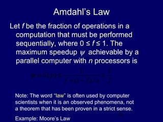
  • 22. 22 Amdahl’s Law Let f be the fraction of operations in a computation that must be performed sequentially, where 0 ≤ f ≤ 1. The maximum speedup ψ achievable by a parallel computer with n processors is fnff pS 1 /)1( 1 )( ≤ −+ ≤≡ψ Note: The word “law” is often used by computer scientists when it is an observed phenomena, not a theorem that has been proven in a strict sense. Example: Moore’s Law
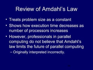
  • 23. 23 Proof for Traditional Problems: If the fraction of the computation that cannot be divided into concurrent tasks is f, and no overhead incurs when the computation is divided into concurrent parts, the time to perform the computation with n processors is given by tp ≥ fts + [(1 - f )ts] / n, as shown below:
  • 24. 24 Proof of Amdahl’s Law (cont.) • Using the preceding expression for tp • The last expression is obtained by dividing numerator and denominator by ts , which establishes Amdahl’s law. n f f n tf ft t t t nS s s s p s )1( 1 )1( )( − + = − + ≤= fn n fnf n nS )1(1)1( )( −+ = −+ ≤
  • 25. 25 Amdahl’s Law • Preceding proof assumes that speedup can not be superliner; i.e., S(n) = ts/ tp ≤ n – Assumption only valid for traditional problems. – Question: Where is this assumption used? • The pictorial portion of this argument is taken from chapter 1 of Wilkinson and Allen • Sometimes Amdahl’s law is just stated as S(n) ≤ 1/f • Note that S(n) never exceeds 1/f and approaches 1/f as n increases.
  • 26. 26 Consequences of Amdahl’s Limitations to Parallelism • For a long time, Amdahl’s law was viewed as a fatal limit to the usefulness of parallelism. • Amdahl’s law is valid for traditional problems and has several useful interpretations. • Some textbooks show how Amdahl’s law can be used to increase the efficient of parallel algorithms – See Reference (16), Jordan & Alaghband textbook • Amdahl’s law shows that efforts required to further reduce the fraction of the code that is sequential may pay off in large performance gains. • Hardware that achieves even a small decrease in the percent of things executed sequentially may be considerably more efficient.
  • 27. 27 Limitations of Amdahl’s Law – A key flaw in past arguments that Amdahl’s law is a fatal limit to the future of parallelism is • Gustafon’s Law: The proportion of the computations that are sequential normally decreases as the problem size increases. – Note Gustafon’s law is a “observed phenomena” and not a theorem. – Other limitations in applying Amdahl’s Law: • Its proof focuses on the steps in a particular algorithm, and does not consider that other algorithms with more parallelism may exist • Amdahl’s law applies only to ‘standard’ problems were superlinearity can not occur
  • 28. 28 Example 1 • 95% of a program’s execution time occurs inside a loop that can be executed in parallel. What is the maximum speedup we should expect from a parallel version of the program executing on 8 CPUs? 9.5 8/)05.01(05.0 1 ≅ −+ ≤ψ
  • 29. 29 Example 2 • 5% of a parallel program’s execution time is spent within inherently sequential code. • The maximum speedup achievable by this program, regardless of how many PEs are used, is 20 05.0 1 /)05.01(05.0 1 lim == −+∞→ pp
  • 30. 30 Pop Quiz • An oceanographer gives you a serial program and asks you how much faster it might run on 8 processors. You can only find one function amenable to a parallel solution. Benchmarking on a single processor reveals 80% of the execution time is spent inside this function. What is the best speedup a parallel version is likely to achieve on 8 processors? Answer: 1/(0.2 + (1 - 0.2)/8) ≅ 3.3
  • 31. 31 Another Limitation of Amdahl’s Law • Ignores communication cost κ(n,p) • On communications-intensive applications, the κ(n,p) does not capture the additional communication slowdown due to network congestion. • As a result, Amdahl’s law usually overestimates speedup achievable
  • 32. 32 Amdahl Effect • Typically communications time κ(n,p) has lower complexity than ϕ(n)/p (i.e., time for parallel part) • As n increases, ϕ(n)/p dominates κ(n,p) • As n increases, – sequential portion of algorithm decreases – speedup increases
  • 33. 33 Illustration of Amdahl Effect n = 100 n = 1,000 n = 10,000 Speedup Processors
  • 34. 34 Review of Amdahl’s Law • Treats problem size as a constant • Shows how execution time decreases as number of processors increases • However, professionals in parallel computing do not believe that Amdahl’s law limits the future of parallel computing – Originally interpreted incorrectly.
  • 35. 35 Summary (1) • Performance terms – Running Time – Cost – Efficiency – Speedup • Model of speedup – Serial component – Parallel component – Communication component
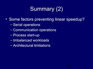
  • 36. 36 Summary (2) • Some factors preventing linear speedup? – Serial operations – Communication operations – Process start-up – Imbalanced workloads – Architectural limitations