Computational hydraulics
5 likes3,212 views

This document provides an overview of computational hydraulics and open channel flows. It covers basic concepts like pressure, velocity, and total head. It also discusses key conservation laws like mass, momentum, and energy. The document defines different types of open channel flows such as subcritical, critical, supercritical, gradually varied, rapidly varied, steady, and unsteady flows. It provides examples and definitions for concepts like specific energy, specific force, uniform flows, critical flows, and gradually varied flow profiles. Finally, it discusses rapidly varied and unsteady flows with examples.


![Matrix notation
Matrix : a rectangular array (n x m) of numbers
⎡ a11 a12 . . . a1m ⎤
⎢a21 a22 . . . a2 m ⎥
⎢ . ⎥
[ ]
A = aij = ⎢ .
⎢ . . ⎥
⎥
⎢ . . ⎥
⎢ an1 an 2 . . . anm ⎥
⎣ ⎦ nxm
Matrix Addition:
C = A+B = [aij+ bij] = [cij], where cij = aij + bij
Matrix Multiplication:
AB = C = [aij][bij] = [cij], where
m
cij = ∑ aik bkj i = 1,2,..., n, j = 1,2,..., r.
k =1](https://image.slidesharecdn.com/computational-hydraulics-120528214006-phpapp01/85/Computational-hydraulics-94-320.jpg)


![Matrix Inversion
Sometimes the problem of solving the linear
algebraic system is loosely referred to as matrix
inversion
Matrix inversion means, given a square matrix [A]
with nonzero determinant, finding a second
matrix [A-1] having the property that [A-1][A]=[I],
[I] is the identity matrix
[A]x=c
x= [A-1]c
[A-1][A]=[I]=[A][A-1]](https://image.slidesharecdn.com/computational-hydraulics-120528214006-phpapp01/85/Computational-hydraulics-121-320.jpg)


![Picard’s technique of linearization
Where [T yi , j + T yi , j +1 ]
Bi, j = −
2∆y 2
[Txi , j + Txi −1, j ]
Di, j = −
2∆x 2
[Txi , j + Txi +1, j ]
Fi, j = −
2∆x 2
[T yi , j + T yi , j +1 ]
H i, j = −
2∆y 2](https://image.slidesharecdn.com/computational-hydraulics-120528214006-phpapp01/85/Computational-hydraulics-133-320.jpg)


![Derivatives
Derivatives from difference tables
We use the divided difference table to estimate values for
derivatives. Interpolating polynomial of degree n that fits at
points p0,p1,…,pn in terms of divided differences,
f ( x) = Pn ( x) + error
= f [ x0 ] + f [ x0 , x1 ]( x − x0 )
+ f [ x0 , x1, x 2]( x − x0 )( x − x1 )
+ ... + f [ x0 , x1,..., xn ] ∏( x − xi )
+ error
Now we should get a polynomial that approximates the
derivative,f’(x), by differentiating it
Pn ' ( x) = f [ x0 , x1 ] + f [ x0 , x1, x2 ][( x − x1) + ( x − x0 )]
n −1 ( x − x )( x − x )...( x − x
+ ... + f [ x0 , x1,...xn ] ∑ 0 1 n −1 )
i =0 ( x − xi )](https://image.slidesharecdn.com/computational-hydraulics-120528214006-phpapp01/85/Computational-hydraulics-145-320.jpg)
![Derivatives continued
To get the error term for the above approximation, we
have to differentiate the error term for Pn(x), the error term
for Pn(x):
f ( n +1) (ξ )
Error = ( x − x0 )( x − x1)...( x − xn ) .
(n + 1)!
ξ
Error of the approximation to f’(x), when x=xi, is
⎡ ⎤
⎢ n ⎥ f ( n +1) (ξ )
Error = ⎢ ∏ ( xi − x j )⎥ , ξ in [x,x0,xn].
⎢ j =0 ⎥ (n + 1)!
⎢ j ≠i
⎣ ⎥
⎦
Error is not zero even when x is a tabulated value, in fact
the error of the derivative is less at some x-values between
the points](https://image.slidesharecdn.com/computational-hydraulics-120528214006-phpapp01/85/Computational-hydraulics-146-320.jpg)
![Derivatives continued
Evenly spaced data
When the data are evenly spaced, we can use a table of
function differences to construct the interpolating
polynomial.
( x − xi )
We use in terms of: s=
h
s ( s − 1) 2 s ( s − 1)( s − 2) 3
Pn ( s ) = f i + s∆f i + ∆ fi + ∆ fi
2! 3!
n −1 ∆n f i
+ ... + ∏ ( s − j ) + error ;
j =0 n!
⎡ n ⎤ f ( n +1) (ξ )
Error = ⎢ ∏ ( s − j )⎥ ,
⎢ j =0 ⎥ (n + 1)! ξ in [x,x0,xn].
⎣ ⎦](https://image.slidesharecdn.com/computational-hydraulics-120528214006-phpapp01/85/Computational-hydraulics-147-320.jpg)
![Derivatives continued
The derivative of Pn(s) should approximate f’(x)
d d ds
Pn ( s ) = Pn ( s )
dx ds dx
⎡ ⎧ ⎫ ⎤
1⎢ n ⎪ j −1 j −1
⎪ ⎪ ∆ j fi ⎥
⎪
= ⎢∆fi + ∑ ⎨ ∑ ∏ ( s − l )⎬ ⎥.
h⎢ j = 2 ⎪k = 0 l = 0 ⎪ j! ⎥
⎢ ⎪
⎩ l ≠k ⎪
⎭ ⎥
⎣ ⎦
ds d ( x − xi ) 1
Where = =
dx dx h h
(−1) n h n ( n +1)
When x=xi, s=0 Error = f (ξ ), ξ in [x1,…, xn].
n +1](https://image.slidesharecdn.com/computational-hydraulics-120528214006-phpapp01/85/Computational-hydraulics-148-320.jpg)
![Derivatives continued
Simpler formulas
Forward difference approximation
For an estimate of f’(xi), we get
1 1 1 1
f ' ( x) = [∆f i − ∆2 f i + ∆3 fi − ... ± ∆n fi ] x = xi
h 2 3 n
With one term, linearly interpolating, using a polynomial of
degree 1, we have (error is O(h))
' 1 1 "
f ( xi ) = [∆f i ] − hf (ξ ),
h 2
With two terms, using a polynomial of degree 2, we have
(error is O(h2))
1⎡ 1 ⎤ 1
f ' ( xi ) = ∆f i − ∆2 f i ⎥ + h 2 f (3) (ξ ),
h⎢
⎣ 2 ⎦ 3](https://image.slidesharecdn.com/computational-hydraulics-120528214006-phpapp01/85/Computational-hydraulics-149-320.jpg)


![Newton-Cotes integration formulas
To develop the Newton-Cotes formulas, change the
variable of integration from x to s. Also dx = hds
For any f(x), assume a polynomial Pn(xs) of degree 1 i.e
n=1
x1 x1
∫ f ( x)dx = ∫ ( f 0 + s∆f 0 )dx
x0 x0
s =1
= h ∫ ( f 0 + s∆f 0 )ds
s =0
1
2⎤
s 1
= hf 0 s ]1 + h∆f 0
0 ⎥ = h( f 0 + ∆f 0 )
2⎥ 2
⎦0
h h
= [2 f 0 + ( f1 − f 0 )] = ( f 0 + f1 )
2 2](https://image.slidesharecdn.com/computational-hydraulics-120528214006-phpapp01/85/Computational-hydraulics-154-320.jpg)


![Trapezoidal and Simpson’s rule cont…
Trapezoidal rule-a composite formula
The first of the Newton-Cotes formulas, based on
approximating f(x) on (x0,x1) by a straight line, is
trapezoidal rule
xi +1 f ( xi ) + f ( xi +1 ) h
∫ f ( x)dx = (∆x) = ( f i + f i +1 ),
xi 2 2
For [a,b] subdivided into n subintervals of size h,
b n h h
∫ f ( x)dx = ∑ ( f i + f i +1 ) = ( f1 + f 2 + f 2 + f 3 + ... + f n + f n +1 );
a i =12 2
b h
∫ f ( x)dx = ( f1 + 2 f 2 + 2 f 3 + ... + 2 f n + f n +1 ).
a 2](https://image.slidesharecdn.com/computational-hydraulics-120528214006-phpapp01/85/Computational-hydraulics-158-320.jpg)

![Trapezoidal and Simpson’s rule cont…
Trapezoidal rule-a composite formula cont…
1 3 "
Local error =− h f (ξ1 ), x0 < ξ1 < x1
12
Global error 1 3 "
= − h [ f (ξ1 ) + f " (ξ 2 ) + ... + f " (ξ n )],
12
If we assume that f”(x) is continuous on (a,b), there is
some value of x in (a,b), say x=ξ, at which the value of the
sum in above equation is equal to n.f”(ξ), since nh=b-a, the
global error becomes
Global error
1 3 " −(b − a ) 2 "
= − h nf (ξ ) = h f (ξ ) = O(h 2 ).
12 12
The error is of 2nd order in this case](https://image.slidesharecdn.com/computational-hydraulics-120528214006-phpapp01/85/Computational-hydraulics-160-320.jpg)

![Trapezoidal and Simpson’s rule
Simpson’s rule
The composite Newton-Cotes formulas based on
quadratic and cubic interpolating polynomials are
known as Simpson’s rule
1
Quadratic- Simpson’s 3
rule
The second degree Newton-Cotes formula
integrates a quadratic over two intervals of equal
width, h h
f ( x)dx = [ f0 + 4 f1 + f 2 ].
3
This formula has a local error of O(h5):
1 5 ( 4)
Error = − h f (ξ )
90](https://image.slidesharecdn.com/computational-hydraulics-120528214006-phpapp01/85/Computational-hydraulics-162-320.jpg)
![Trapezoidal and Simpson’s rule
Quadratic- Simpson’s 1
3 rule cont…
For [a,b] subdivided into n (even) subintervals of
size h,
h
f ( x)dx = [ f (a ) + 4 f1 + 2 f 2 + 4 f 3 + 2 f 4 + ... + 4 f n −1 + f (b)].
3
With an error of
(b − a ) 4 ( 4)
Error = − h f (ξ )
180
We can see that the error is of 4 th order
The denominator changes to 180, because we
integrate over pairs of panels, meaning that the
local rule is applied n/2 times](https://image.slidesharecdn.com/computational-hydraulics-120528214006-phpapp01/85/Computational-hydraulics-163-320.jpg)
![Trapezoidal and Simpson’s rule
Cubic- Simpson’s 3
8
rule
The composite rule based on fitting four points
with a cubic leads to Simpson’s 3 rule
8
For n=3 from Newton’s Cotes formula we get
3h
f ( x)dx = [ f0 + 3 f1 + 3 f 2 + f3 ].
8
3 5 ( 4)
Error = − h f (ξ )
80
The local order of error is same as 1/3 rd rule,
except the coefficient is larger](https://image.slidesharecdn.com/computational-hydraulics-120528214006-phpapp01/85/Computational-hydraulics-164-320.jpg)
![Trapezoidal and Simpson’s rule
Cubic- Simpson’s 3
8
rule cont…
To get the composite rule for [a,b] subdivided into
n (n divisible by 3) subintervals of size h,
3h
f ( x)dx = [ f (a ) + 3 f1 + 3 f 2 + 2 f 3 + 3 f 4 + 3 f 5 + 2 f 6
8
+ ... + 2 f n −3 + 3 f n − 2 + 3 f n −1 + f (b)]
With an error of
(b − a ) 4 ( 4)
Error = − h f (ξ )
80](https://image.slidesharecdn.com/computational-hydraulics-120528214006-phpapp01/85/Computational-hydraulics-165-320.jpg)


![Multi-step methods
We have the formula to advance y:
h
yn +1 = yn + [23 f n − 16 f n −1 + 5 f n − 2 ] + O(h 4 )
12
This formula resembles the single step formulas,
in that the increment to y is a weighted sum of
the derivatives times the step size, but differs in
that past values are used rather than estimates in
the forward direction.
We can reduce the error by using more past
points for fitting a polynomial](https://image.slidesharecdn.com/computational-hydraulics-120528214006-phpapp01/85/Computational-hydraulics-192-320.jpg)
![Multi-step methods
In fact, when the derivation is done for four
points to get a cubic approximation to
f(x,y), the following is obtained
h
yn +1 = yn + [55 f n − 59 f n −1 + 37 f n − 2 − 9 f n −3 ] + O(h5 )
24](https://image.slidesharecdn.com/computational-hydraulics-120528214006-phpapp01/85/Computational-hydraulics-193-320.jpg)


![Multi-step methods
Adam-Moulton Method, more stable than and as
efficient as Milne method .
Adam-Moulton predictor formula:
h 251 5 v
yn +1 = yn + [55 f n − 59 f n −1 + 37 f n − 2 − 9 f n −3 ] + h y (ξ1 )
24 720
Adam-Moulton corrector formula:
h 19 5 v
yn +1 = yn + [9 f n +1 + 19 f n − 5 f n −1 + f n − 2 ] − h y (ξ 2 )
24 720
The efficiency of this method is about twice that
of Runge-Kutta and Runge-kutta Fehlberg
methods](https://image.slidesharecdn.com/computational-hydraulics-120528214006-phpapp01/85/Computational-hydraulics-197-320.jpg)


![Types of FD techniques cont…
This approximation is referred to as central finite difference
approximation
Error term is of order O(∆x)2, known as second order
accurate
Central-difference approximations to derivates are more
accurate than forward or backward approximations [O(h2)
verses O(h)]
Consider FD approximation for partial derivative](https://image.slidesharecdn.com/computational-hydraulics-120528214006-phpapp01/85/Computational-hydraulics-219-320.jpg)


![FD Approximation of PDEs
It is convenient to use double subscript on u to
indicate the x- and y- values:
2 ui +1, j − 2ui, j + ui −1, j ui, j +1 − 2ui, j + ui, j −1
∇ ui , j = + = 0.
(∆x) 2 (∆y ) 2
For the sake of simplification, it is usual to take
∆x= ∆y=h
2
∇ ui , j =
1
u [
2 i +1, j
+ ui −1, j + ui, j +1 + ui, j −1 − 4ui, j = 0. ]
h
We can notice that five points are involved in the
above relation, known as five point star formula](https://image.slidesharecdn.com/computational-hydraulics-120528214006-phpapp01/85/Computational-hydraulics-255-320.jpg)


![CGHS method
A symmetric matrix A is said to be positive
definite if xTAx>0 whenever x≠0 where x is
any column vector. So the resulting
conjugate gradient method minimizes the A
norm of the error vector (i.e. ei +1 A ).
The convergence of conjugate gradient
method depend upon the distribution of
eigenvalues of matrix A and to a lesser
extend upon the condition number [k(A)] of
the matrix. The condition number of a
symmetric positive definite matrix is defined
as k ( A ) = λmax / λmin](https://image.slidesharecdn.com/computational-hydraulics-120528214006-phpapp01/85/Computational-hydraulics-273-320.jpg)


![Solution of gradually varied flows
A better estimate for y2 can be computed from the
equation *
F ( y2 )
y2 = y* −
2
[dF / dy2 ]*
If y2 − y*
2 is less than a specified tolerance, ε, then
y*
2 is the flow depth y2, at section 2; otherwise,
set y* = y2
2 and repeat the steps until a solution
is obtained](https://image.slidesharecdn.com/computational-hydraulics-120528214006-phpapp01/85/Computational-hydraulics-314-320.jpg)


![Solution of gradually varied flows cont..
3. Improved Euler method
Let us call the flow depth at xi +1 obtained by using Euler
method as y * i.e.,
i +1
*
yi +1 = yi + yi' ∆x
By using this value, we can compute the slope of the curve
(
y = y (x) at x = xi +1 , i.e., yi' +1 = f xi +1 , yi*+1 . Let us )
use the average value of the slopes of the curve at xi and
xi +1 . Then we can determine the value of yi +1 from the
equation yi +1 = yi +
2
(
1 '
)
yi + yi' +1 ∆x . This equation may be
yi +1 = yi +
1
[ ]
f ( xi , yi ) + f ( xi +1 , yi*+1 ) ∆x
written as 2 . This method
called the improved Euler method, is second order accurate.](https://image.slidesharecdn.com/computational-hydraulics-120528214006-phpapp01/85/Computational-hydraulics-320-320.jpg)

![Solution of gradually varied flows cont..
Predictor-corrector methods
In this method we predict the unknown flow depth first,
correct this predicted value, and then re-correct this
corrected value. This iteration is continued till the desired
accuracy is met.
In the predictor part, let us use the Euler method to
predict the value of yi+1, I.e
yi(+1 = yi + f ( xi , yi )∆x
0)
we may correct using the following equation
1
yi +1 = yi + [ f ( xi , yi ) + f ( xi +1, yi(+1 )]∆x
(1) 0)
2](https://image.slidesharecdn.com/computational-hydraulics-120528214006-phpapp01/85/Computational-hydraulics-322-320.jpg)
![Solution of gradually varied flows cont..
Now we may re-correct y again to obtain a better
value:
1
yi(+1 = yi +
2)
[ f ( xi , yi ) + f ( xi +1, yi(1) )]∆x
+1
2
Thus the j th iteration is
1 j−
yi(+1 = yi +
j)
[ f ( xi , yi ) + f ( xi +1, yi(+1 1) )]∆x
2
Iteration until j−
yi(+1 − yi(+1 1) ≤ ε
j) , where ε = specified
tolerance](https://image.slidesharecdn.com/computational-hydraulics-120528214006-phpapp01/85/Computational-hydraulics-323-320.jpg)


![FD methods for Saint Venant equations
Continued…
n +1 n +1 n n
∂f α ( f i +1 + f i ) (1 − α )( f i +1 + f i )
= +
∂x ∆x ∆x
1 1
f = α ( f in +1 + fin +1 ) + (1 − α )( f in 1 + f in )
+1 +
2 2
U in +1 + U in +1 = 2
+1
∆t
∆x
[
α ( Fin +1 − Fin +1) + (1 − α )( Fin 1 − Fin )
+1 + ]
[
+ ∆t α ( Sin +1 + Sin +1 ) + (1 − α )( Sin 1 + Sin )
+1 + ]
= U in + U in 1
+](https://image.slidesharecdn.com/computational-hydraulics-120528214006-phpapp01/85/Computational-hydraulics-328-320.jpg)


![Solution procedure
The expansion of the equation…
ain +1 + ain +1 + 2
+1
∆t
∆x
{[ ] [
α (va)i +1 − (va)i +1 + (1 − α ) (va)i +1 − (va)i
n +1 n n n
]}
= ain + ain 1
+
(va)i +1 + (va)i +1 + 2
n n +1 ∆t
∆x
{[
α (v 2 a + gay )i +1 − (v 2 a + gay )i +1
n +1 n
]}
{[
− ga∆t α ( s0 − s f )i +1 + ( s0 − s f )i +1
n +1 n
]}
= ga∆t {1 − α )[( s
( 0
n n
− s f )i +1 + ( s0 − s f )i ]}
+ (va)i + (va)i +1 − (1 − α ) 2
n n ∆t 2
∆x
{
(v a + gay )i +1 − (v 2 a + gay )i
n n
}
The above set of nonlinear algebraic equations
can be solved by Newton-Raphson method](https://image.slidesharecdn.com/computational-hydraulics-120528214006-phpapp01/85/Computational-hydraulics-331-320.jpg)


![Method of characteristics
These equations can be written in terms of velocity
1 ∂v ∂H f
L1 = + + vv = 0
g ∂t ∂x 2 Dg
∂H a 2 ∂v
L2 = + =0
∂t g ∂x
Where,
k
a=
e[1 + (kD / ρE )]](https://image.slidesharecdn.com/computational-hydraulics-120528214006-phpapp01/85/Computational-hydraulics-341-320.jpg)


![Network Analysis
2. Energy conservation equations – the energy conservation
equations state that the energy loss along a path equals
the difference in head at the starting node and end node
of the path.
∑ (± )h( p) + ∑ (± )h( p) − [H (s(l )) − H (e(l ))] = 0 l = 1,..., NL + NPATH
pε {l} pε {l}
Where h(p) is the head loss in element p(m), s(l) is the
starting node of path l, e(l) is the end of path 1, NL is the
number of loops, and NPATH is the number of paths other
than loops and pε {l} refers to the pipes belonging to path
l. loop is a special case of path, wherein, the starting node
and end node are the same, making the head loss around
a loop zero, that is,
∑ (± )h( p) + ∑ (± )h( p) = 0](https://image.slidesharecdn.com/computational-hydraulics-120528214006-phpapp01/85/Computational-hydraulics-357-320.jpg)


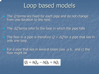
![Loop based models
The loop energy equations may be written
ml
F (∆Q) = ∑ K i [sgn(Qii + ∆Ql )] Qii + ∆Ql
n
= dhl (l=1,2,…,L)
i =1
Where
Qii = initial estimate of the flow in i th pipe, L3/T
∆Ql = correction to flow in l th loop, L3/T
ml = number of pipes in l th loop
L = number of loops](https://image.slidesharecdn.com/computational-hydraulics-120528214006-phpapp01/85/Computational-hydraulics-367-320.jpg)


![Solution of pipe network problems
through Newton-Raphson method
New value of x+∆x becomes x for the next iteration. This
process is continued until F is sufficiently close to zero
For a pipe network problem, this method can be applied to
the N-1=k, H-equations
The head (H) equations for each node (1 through k), it is
possible to write as:
1 / nij
⎛ H −H ⎞
[ ]
mi ⎜ j i ⎟
F ( H i ) = ∑ sgn( H j − H i ) ⎜ − Ui = 0 (i = 1,2,..., K )
⎟
j =1 ⎜ K ji ⎟
⎝ ⎠
Where mi= number of pipes connected to node I
Ui= consumptive use at node i, L3/T
F(i) and F(i+1) is the value of F at ith and (i+1)th iteration,
then
dF = F (i + 1) − F (i )](https://image.slidesharecdn.com/computational-hydraulics-120528214006-phpapp01/85/Computational-hydraulics-371-320.jpg)

![Solution of pipe network problems
through Newton-Raphson method
Initial guess for H
Calculate partial derivatives of each F with respect to each H
Solving the resulting system of linear equations to find H,
and repeating until all of the F’s are sufficiently close to 0
The derivative of the terms in the previous equation is
given by
1 / nij
⎛ H −H ⎞
d
[ ( )]
⎜ i
sgn H i − H j ⎜
j ⎟
=
−1
(H i − H j )(1 / n )−1
(nij )(Kij )1 / n
ij
dH j K ij ⎟
⎜ ⎟ ij
⎝ ⎠
1 / nij
and ⎛ H −H ⎞
d
[ ( )]
⎜ i
sgn H i − H j ⎜
j ⎟
=
1
(H i − H j )(1 / n )−1
(nij )(Kij )1 / n
ij
dH i K ij ⎟
⎜ ⎟ ij
⎝ ⎠](https://image.slidesharecdn.com/computational-hydraulics-120528214006-phpapp01/85/Computational-hydraulics-373-320.jpg)

![Solution of pipe network problems
through Hardy-Cross method
Nevertheless it is still widely used especially for manual
solutions and small computers or hand calculators and
produces adequate results for most problems
For the l th loop in a pipe network the ∆Q equation can be
written as follows
ml
F (∆Q1 ) = ∑ K i [sgn (Qii + ∆Ql )] Qii + ∆Ql
n
− dhl = 0
i =1
Where
∆Ql=correction to l th loop to achieve convergence, L3/T
Qii=initial estimates of flow in i th pipe (satisfies
continuity),L3/T
ml=number of pipes in loop l](https://image.slidesharecdn.com/computational-hydraulics-120528214006-phpapp01/85/Computational-hydraulics-375-320.jpg)


![Assignments continued
1
2
8 2 1 - Node with H unknown & C known
- Node with H known & C known
3 4
- Node with H known & C unknown
- Node with R unknown
5
3 4
- Pump element
Unknowns
6 7
H [2], H [4], H [5]
R [4], R [5]
C [6], C [7], C [8]
7 5 6
8 9](https://image.slidesharecdn.com/computational-hydraulics-120528214006-phpapp01/85/Computational-hydraulics-379-320.jpg)


Computational hydraulics
- 1. Computational Hydraulics Prof. M.S.Mohan Kumar Department of Civil Engineering
- 2. Introduction to Hydraulics of Open Channels Module 1 3 lectures
- 3. Topics to be covered Basic Concepts Conservation Laws Critical Flows Uniform Flows Gradually Varied Flows Rapidly Varied Flows Unsteady Flows
- 4. Basic Concepts Open Channel flows deal with flow of water in open channels Pressure is atmospheric at the water surface and the pressure is equal to the depth of water at any section Pressure head is the ratio of pressure and the specific weight of water Elevation head or the datum head is the height of the section under consideration above a datum Velocity head (=v2/2g) is due to the average velocity of flow in that vertical section
- 5. Basic Concepts Cont… Total head =p/γ + v2/2g + z Pressure head = p/γ Velocity head =v2/2g Datum head = z The flow of water in an open channel is mainly due to head gradient and gravity Open Channels are mainly used to transport water for irrigation, industry and domestic water supply
- 6. Conservation Laws The main conservation laws used in open channels are Conservation Laws Conservation of Mass Conservation of Momentum Conservation of Energy
- 7. Conservation of Mass Conservation of Mass In any control volume consisting of the fluid ( water) under consideration, the net change of mass in the control volume due to inflow and out flow is equal to the the net rate of change of mass in the control volume This leads to the classical continuity equation balancing the inflow, out flow and the storage change in the control volume. Since we are considering only water which is treated as incompressible, the density effect can be ignored
- 8. Conservation of Momentum and energy Conservation of Momentum This law states that the rate of change of momentum in the control volume is equal to the net forces acting on the control volume Since the water under consideration is moving, it is acted upon by external forces Essentially this leads to the Newton’s second law Conservation of Energy This law states that neither the energy can be created or destroyed. It only changes its form.
- 9. Conservation of Energy Mainly in open channels the energy will be in the form of potential energy and kinetic energy Potential energy is due to the elevation of the water parcel while the kinetic energy is due to its movement In the context of open channel flow the total energy due these factors between any two sections is conserved This conservation of energy principle leads to the classical Bernoulli’s equation P/γ + v2/2g + z = Constant When used between two sections this equation has to account for the energy loss between the two sections which is due to the resistance to the flow by the bed shear etc.
- 10. Types of Open Channel Flows Depending on the Froude number (Fr) the flow in an open channel is classified as Sub critical flow, Super Critical flow, and Critical flow, where Froude number can be defined as F = V r gy Open channel flow Sub-critical flow Sub- Critical flow Super critical flow Fr<1 Fr=1 Fr>1
- 11. Types of Open Channel Flow Cont... Open Channel Flow Unsteady Steady Varied Uniform Varied Gradually Gradually Rapidly Rapidly
- 12. Types of Open Channel Flow Cont… Steady Flow Flow is said to be steady when discharge does not change along the course of the channel flow Unsteady Flow Flow is said to be unsteady when the discharge changes with time Uniform Flow Flow is said to be uniform when both the depth and discharge is same at any two sections of the channel
- 13. Types of Open Channel Cont… Gradually Varied Flow Flow is said to be gradually varied when ever the depth changes gradually along the channel Rapidly varied flow Whenever the flow depth changes rapidly along the channel the flow is termed rapidly varied flow Spatially varied flow Whenever the depth of flow changes gradually due to change in discharge the flow is termed spatially varied flow
- 14. Types of Open Channel Flow cont… Unsteady Flow Whenever the discharge and depth of flow changes with time, the flow is termed unsteady flow Types of possible flow Steady uniform flow Steady non-uniform flow Unsteady non-uniform flow kinematic wave diffusion wave dynamic wave
- 15. Definitions Specific Energy It is defined as the energy acquired by the water at a section due to its depth and the velocity with which it is flowing Specific Energy E is given by, E = y + v2/2g Where y is the depth of flow at that section and v is the average velocity of flow Specific energy is minimum at critical condition
- 16. Definitions Specific Force It is defined as the sum of the momentum of the flow passing through the channel section per unit time per unit weight of water and the force per unit weight of water F = Q2/gA +yA The specific forces of two sections are equal provided that the external forces and the weight effect of water in the reach between the two sections can be ignored. At the critical state of flow the specific force is a minimum for the given discharge.
- 17. Critical Flow Flow is critical when the specific energy is minimum. Also whenever the flow changes from sub critical to super critical or vice versa the flow has to go through critical condition figure is shown in next slide Sub-critical flow-the depth of flow will be higher whereas the velocity will be lower. Super-critical flow-the depth of flow will be lower but the velocity will be higher Critical flow: Flow over a free over-fall
- 18. Specific energy diagram E=y Depth of water Surface (y) E-y curve 1 Emin y1 C Alternate Depths c 2 y 45° 2 Critical Depth Specific Energy (E) y Specific Energy Curve for a given discharge
- 19. Characteristics of Critical Flow Specific Energy (E = y+Q2/2gA2) is minimum For Specific energy to be a minimum dE/dy = 0 dE Q 2 dA = 1− 3 ⋅ dy gA dy However, dA=Tdy, where T is the width of the channel at the water surface, then applying dE/dy = 0, will result in following Q 2Tc Ac Q2 Ac VC2 =1 = 2 = gAc 3 Tc gAc Tc g
- 20. Characteristics of Critical Flow For a rectangular channel Ac /Tc=yc Following the derivation for a rectangular channel, Vc Fr = =1 gy c The same principle is valid for trapezoidal and other cross sections Critical flow condition defines an unique relationship between depth and discharge which is very useful in the design of flow measurement structures
- 21. Uniform Flows This is one of the most important concept in open channel flows The most important equation for uniform flow is Manning’s equation given by 1 2 / 3 1/ 2 V= R S n Where R = the hydraulic radius = A/P P = wetted perimeter = f(y, S0) Y = depth of the channel bed S0 = bed slope (same as the energy slope, Sf) n = the Manning’s dimensional empirical constant
- 22. Uniform Flows Energy Grade Line 2 V12/2g 1 1 hf Sf v22/2g y1 Control Volume y2 So 1 z1 z2 Datum Steady Uniform Flow in an Open Channel
- 23. Uniform Flow Example : Flow in an open channel This concept is used in most of the open channel flow design The uniform flow means that there is no acceleration to the flow leading to the weight component of the flow being balanced by the resistance offered by the bed shear In terms of discharge the Manning’s equation is given by 1 Q = AR 2 / 3 S 1/ 2 n
- 24. Uniform Flow This is a non linear equation in y the depth of flow for which most of the computations will be made Derivation of uniform flow equation is given below, where W sin θ = weight component of the fluid mass in the direction of flow τ0 = bed shear stress P∆x = surface area of the channel
- 25. Uniform Flow The force balance equation can be written as W sin θ − τ 0 P∆x = 0 Or γA∆x sin θ − τ 0 P∆x = 0 A Or τ 0 = γ sin θ P Now A/P is the hydraulic radius, R, and sinθ is the slope of the channel S0
- 26. Uniform Flow The shear stress can be expressed as τ 0 = c f ρ (V 2 / 2) Where cf is resistance coefficient, V is the mean velocity ρ is the mass density Therefore the previous equation can be written as V2 2g Or cf ρ = γRS 0 V = RS 0 = C RS 0 2 cf where C is Chezy’s constant For Manning’s equation 1.49 1 / 6 C= R n
- 27. Gradually Varied Flow Flow is said to be gradually varied whenever the depth of flow changed gradually The governing equation for gradually varied flow is given by dy S 0 − S f = dx 1 − Fr 2 Where the variation of depth y with the channel distance x is shown to be a function of bed slope S0, Friction Slope Sf and the flow Froude number Fr. This is a non linear equation with the depth varying as a non linear function
- 28. Gradually Varied Flow Energy-grade line (slope = Sf) v2/2g Water surface (slope = Sw) y Channel bottom (slope = So) z Datum Total head at a channel section
- 29. Gradually Varied Flow Derivation of gradually varied flow is as follows… The conservation of energy at two sections of a reach of length ∆x, can be written as 2 2 V1 V2 y1 + + S 0 ∆x = y 2 + + S f ∆x 2g 2g Now, let ∆y = y − y and V2 2 V1 2 d ⎛ V 2 ⎞ 2 1 − = ⎜⎜ ⎟∆x ⎟ 2g 2g dx ⎝ 2 g ⎠ Then the above equation becomes d ⎛V 2 ⎞ ∆y = S 0 ∆x − S f ∆x − ⎜ ⎜ 2 g ⎟∆x ⎟ dx ⎝ ⎠
- 30. Gradually Varied Flow Dividing through ∆x and taking the limit as ∆x approaches zero gives us dy d ⎛ V 2 ⎞ + ⎜ ⎜ 2g ⎟ = S0 − S f ⎟ dx dx ⎝ ⎠ After simplification, dy S0 − S f = ( ) dx 1 + d V 2 / 2 g / dy Further simplification can be done in terms of Froude number d ⎛V 2 ⎞ d ⎛ Q2 ⎞ ⎜ ⎜ 2 g ⎟ = dy ⎜ 2 gA 2 ⎟ ⎜ ⎟ ⎟ dy ⎝ ⎠ ⎝ ⎠
- 31. Gradually Varied Flow After differentiating the right side of the previous equation, d ⎛ V ⎞ − 2Q dA 2 2 ⎜ 2 g ⎟ = 2 gA 3 ⋅ dy ⎜ ⎟ dy ⎝ ⎠ But dA/dy=T, and A/T=D, therefore, d ⎛V 2 ⎞ − Q2 ⎜ ⎟= = − Fr 2 dy ⎜ 2 g ⎟ gA 2 D ⎝ ⎠ Finally the general differential equation can be written as dy S 0 − S f = dx 1 − Fr 2
- 32. Gradually Varied Flow Numerical integration of the gradually varied flow equation will give the water surface profile along the channel Depending on the depth of flow where it lies when compared with the normal depth and the critical depth along with the bed slope compared with the friction slope different types of profiles are formed such as M (mild), C (critical), S (steep) profiles. All these have real examples. M (mild)-If the slope is so small that the normal depth (Uniform flow depth) is greater than critical depth for the given discharge, then the slope of the channel is mild.
- 33. Gradually Varied Flow C (critical)-if the slope’s normal depth equals its critical depth, then we call it a critical slope, denoted by C S (steep)-if the channel slope is so steep that a normal depth less than critical is produced, then the channel is steep, and water surface profile designated as S
- 34. Rapidly Varied Flow This flow has very pronounced curvature of the streamlines It is such that pressure distribution cannot be assumed to be hydrostatic The rapid variation in flow regime often take place in short span When rapidly varied flow occurs in a sudden-transition structure, the physical characteristics of the flow are basically fixed by the boundary geometry of the structure as well as by the state of the flow Examples: Channel expansion and cannel contraction Sharp crested weirs Broad crested weirs
- 35. Unsteady flows When the flow conditions vary with respect to time, we call it unsteady flows. Some terminologies used for the analysis of unsteady flows are defined below: Wave: it is defined as a temporal or spatial variation of flow depth and rate of discharge. Wave length: it is the distance between two adjacent wave crests or trough Amplitude: it is the height between the maximum water level and the still water level
- 36. Unsteady flows definitions Wave celerity (c): relative velocity of a wave with respect to fluid in which it is flowing with V Absolute wave velocity (Vw): velocity with respect to fixed reference as given below Vw = V ± c Plus sign if the wave is traveling in the flow direction and minus for if the wave is traveling in the direction opposite to flow For shallow water waves c = gy0 where y0=undisturbed flow depth.
- 37. Unsteady flows examples Unsteady flows occur due to following reasons: 1. Surges in power canals or tunnels 2. Surges in upstream or downstream channels produced by starting or stopping of pumps and opening and closing of control gates 3. Waves in navigation channels produced by the operation of navigation locks 4. Flood waves in streams, rivers, and drainage channels due to rainstorms and snowmelt 5. Tides in estuaries, bays and inlets
- 38. Unsteady flows Unsteady flow commonly encountered in an open channels and deals with translatory waves. Translatory waves is a gravity wave that propagates in an open channel and results in appreciable displacement of the water particles in a direction parallel to the flow For purpose of analytical discussion, unsteady flow is classified into two types, namely, gradually varied and rapidly varied unsteady flow In gradually varied flow the curvature of the wave profile is mild, and the change in depth is gradual In the rapidly varied flow the curvature of the wave profile is very large and so the surface of the profile may become virtually discontinuous.
- 39. Unsteady flows cont… Continuity equation for unsteady flow in an open channel ∂V ∂y ∂y D +V + =0 ∂x ∂x ∂t For a rectangular channel of infinite width, may be written ∂q ∂y + =0 ∂x ∂t When the channel is to feed laterally with a supplementary discharge of q’ per unit length, for instance, into an area that is being flooded over a dike
- 40. Unsteady flows cont… The equation ∂Q ∂A + + q' = 0 ∂x ∂t The general dynamic equation for gradually varied unsteady flow is given by: ∂y αV ∂V 1 ∂V ' + + =0 ∂x g ∂x g ∂t
- 41. Review of Hydraulics of Pipe Flows Module2 3 lectures
- 42. Contents General introduction Energy equation Head loss equations Head discharge relationships Pipe transients flows through pipe networks Solving pipe network problems
- 43. General Introduction Pipe flows are mainly due to pressure difference between two sections Here also the total head is made up of pressure head, datum head and velocity head The principle of continuity, energy, momentum is also used in this type of flow. For example, to design a pipe, we use the continuity and energy equations to obtain the required pipe diameter Then applying the momentum equation, we get the forces acting on bends for a given discharge
- 44. General introduction In the design and operation of a pipeline, the main considerations are head losses, forces and stresses acting on the pipe material, and discharge. Head loss for a given discharge relates to flow efficiency; i.e an optimum size of pipe will yield the least overall cost of installation and operation for the desired discharge. Choosing a small pipe results in low initial costs, however, subsequent costs may be excessively large because of high energy cost from large head losses
- 45. Energy equation The design of conduit should be such that it needs least cost for a given discharge The hydraulic aspect of the problem require applying the one dimensional steady flow form of the energy equation: p1 V12 p2 2 V2 + α1 + z1 + h p = + α2 + z2 + ht + hL γ 2g γ 2g Where p/γ =pressure head αV2/2g =velocity head z =elevation head hp=head supplied by a pump ht =head supplied to a turbine hL =head loss between 1 and 2
- 46. Energy equation Energy Grade Line Hydraulic Grade Line z2 v2/2g p/y hp z1 z Pump z=0 Datum The Schematic representation of the energy equation
- 47. Energy equation Velocity head In αV2/2g, the velocity V is the mean velocity in the conduit at a given section and is obtained by V=Q/A, where Q is the discharge, and A is the cross-sectional area of the conduit. The kinetic energy correction factor is given by α, and it is defines as, where u=velocity at any point in the section 3 ∫ u dA α= A V 3A α has minimum value of unity when the velocity is uniform across the section
- 48. Energy equation cont… Velocity head cont… α has values greater than unity depending on the degree of velocity variation across a section For laminar flow in a pipe, velocity distribution is parabolic across the section of the pipe, and α has value of 2.0 However, if the flow is turbulent, as is the usual case for water flow through the large conduits, the velocity is fairly uniform over most of the conduit section, and α has value near unity (typically: 1.04< α < 1.06). Therefore, in hydraulic engineering for ease of application in pipe flow, the value of α is usually assumed to be unity, and the velocity head is then simply V2/2g.
- 49. Energy equation cont… Pump or turbine head The head supplied by a pump is directly related to the power supplied to the flow as given below P = Qγh p Likewise if head is supplied to turbine, the power supplied to the turbine will be P = Qγht These two equations represents the power supplied directly or power taken out directly from the flow
- 50. Energy equation cont… Head-loss term The head loss term hL accounts for the conversion of mechanical energy to internal energy (heat), when this conversion occurs, the internal energy is not readily converted back to useful mechanical energy, therefore it is called head loss Head loss results from viscous resistance to flow (friction) at the conduit wall or from the viscous dissipation of turbulence usually occurring with separated flow, such as in bends, fittings or outlet works.
- 51. Head loss calculation Head loss is due to friction between the fluid and the pipe wall and turbulence within the fluid The rate of head loss depend on roughness element size apart from velocity and pipe diameter Further the head loss also depends on whether the pipe is hydraulically smooth, rough or somewhere in between In water distribution system , head loss is also due to bends, valves and changes in pipe diameter
- 52. Head loss calculation Head loss for steady flow through a straight pipe: τ 0 A w = ∆ pA r ∆p = 4Lτ 0 / D τ 0 = fρ V 2 / 8 ∆p L V2 h = = f γ D 2g This is known as Darcy-Weisbach equation h/L=S, is slope of the hydraulic and energy grade lines for a pipe of constant diameter
- 53. Head loss calculation Head loss in laminar flow: 32Vµ Hagen-Poiseuille equation gives S= D 2 ρg Combining above with Darcy-Weisbach equation, gives f 64 µ f = ρVD Also we can write in terms of Reynolds number 64 f = Nr This relation is valid for Nr<1000
- 54. Head loss calculation Head loss in turbulent flow: In turbulent flow, the friction factor is a function of both Reynolds number and pipe roughness As the roughness size or the velocity increases, flow is wholly rough and f depends on the relative roughness Where graphical determination of the friction factor is acceptable, it is possible to use a Moody diagram. This diagram gives the friction factor over a wide range of Reynolds numbers for laminar flow and smooth, transition, and rough turbulent flow
- 55. Head loss calculation The quantities shown in Moody Diagram are dimensionless so they can be used with any system of units Moody’s diagram can be followed from any reference book MINOR LOSSES Energy losses caused by valves, bends and changes in pipe diameter This is smaller than friction losses in straight sections of pipe and for all practical purposes ignored Minor losses are significant in valves and fittings, which creates turbulence in excess of that produced in a straight pipe
- 56. Head loss calculation Minor losses can be expressed in three ways: 1. A minor loss coefficient K may be used to give head loss as a function of velocity head, V2 h=K 2g 2. Minor losses may be expressed in terms of the equivalent length of straight pipe, or as pipe diameters (L/D) which produces the same head loss. 2 LV h= f D 2g
- 57. Head loss calculation 1. A flow coefficient Cv which gives a flow that will pass through the valve at a pressure drop of 1psi may be specified. Given the flow coefficient the head loss can be calculated as 18.5 × 10⁶ D 4V 2 h= 2 Cv 2 g The flow coefficient can be related to the minor loss coefficient by 18.5 × 10⁶ D 2 K= 2 Cv
- 58. Energy Equation for Flow in pipes Energy equation for pipe flow P V12 P2 V22 z1 + 1 + = z2 + + + hL ρg 2 g ρg 2 g The energy equation represents elevation, pressure, and velocity forms of energy. The energy equation for a fluid moving in a closed conduit is written between two locations at a distance (length) L apart. Energy losses for flow through ducts and pipes consist of major losses and minor losses. Minor Loss Calculations for Fluid Flow V2 hm = K 2g Minor losses are due to fittings such as valves and elbows
- 59. Major Loss Calculation for Fluid Flow Using Darcy-Weisbach Friction Loss Equation Major losses are due to friction between the moving fluid and the inside walls of the duct. The Darcy-Weisbach method is generally considered more accurate than the Hazen-Williams method. Additionally, the Darcy-Weisbach method is valid for any liquid or gas. Moody Friction Factor Calculator
- 60. Major Loss Calculation in pipes Using Hazen-Williams Friction Loss Equation Hazen-Williams is only valid for water at ordinary temperatures (40 to 75oF). The Hazen-Williams method is very popular, especially among civil engineers, since its friction coefficient (C) is not a function of velocity or duct (pipe) diameter. Hazen-Williams is simpler than Darcy- Weisbach for calculations where one can solve for flow- rate, velocity, or diameter
- 61. Transient flow through long pipes Intermediate flow while changing from one steady state to another is called transient flow This occurs due to design or operating errors or equipment malfunction. This transient state pressure causes lots of damage to the network system Pressure rise in a close conduit caused by an instantaneous change in flow velocity
- 62. Transient flow through long pipes If the flow velocity at a point does vary with time, the flow is unsteady When the flow conditions are changed from one steady state to another, the intermediate stage flow is referred to as transient flow The terms fluid transients and hydraulic transients are used in practice The different flow conditions in a piping system are discussed as below:
- 63. Transient flow through long pipes Consider a pipe length of length L Water is flowing from a constant level upstream reservoir to a valve at downstream Assume valve is instantaneously closed at time t=t0 from the full open position to half open position. This reduces the flow velocity through the valve, thereby increasing the pressure at the valve
- 64. Transient flow through long pipes The increased pressure will produce a pressure wave that will travel back and forth in the pipeline until it is dissipated because of friction and flow conditions have become steady again This time when the flow conditions have become steady again, let us call it t1. So the flow regimes can be categorized into 1. Steady flow for t<t0 2. Transient flow for t0<t<t1 3. Steady flow for t>t1
- 65. Transient flow through long pipes Transient-state pressures are sometimes reduced to the vapor pressure of a liquid that results in separating the liquid column at that section; this is referred to as liquid- column separation If the flow conditions are repeated after a fixed time interval, the flow is called periodic flow, and the time interval at which the conditions are repeated is called period The analysis of transient state conditions in closed conduits may be classified into two categories: lumped-system approach and distributed system approach
- 66. Transient flow through long pipes In the lumped system approach the conduit walls are assumed rigid and the liquid in the conduit is assumed incompressible, so that it behaves like a rigid mass, other way flow variables are functions of time only. In the distributed system approach the liquid is assumed slightly compressible Therefore flow velocity vary along the length of the conduit in addition to the variation in time
- 67. Transient flow through long pipes Flow establishment The 1D form of momentum equation for a control volume that is fixed in space and does not change shape may be written as d 2 2 ∑F = ∫ ρ VAdx + ( ρAV ) out − ( ρ AV ) in dt If the liquid is assumed incompressible and the pipe is rigid, then at any instant the velocity along the pipe will be same, ( ρ AV 2 ) in = ( ρ AV 2 ) out
- 68. Transient flow through long pipes Substituting for all the forces acting on the control volume d pA + γAL sin α − τ 0πDL = (V ρ AL ) dt Where p =γ(h-V2/2g) α=pipe slope D=pipe diameter L=pipe length γ =specific weight of fluid τ0=shear stress at the pipe wall
- 69. Transient flow through long pipes Frictional force is replaced by γhfA, and H0=h+Lsin α and hf from Darcy-weisbach friction equation The resulting equation yields: fL V 2 V 2 L dV H0 − − = . D 2g 2g g dt When the flow is fully established, dV/dt=0. The final velocity V0 will be such that ⎡ fL ⎤ V0 2 H 0 = ⎢1 + ⎣ D ⎥ 2g ⎦ We use the above relationship to get the time for flow to establish 2 LD dV dt = . D + fL V02 − V 2
- 70. Transient flow through long pipes Change in pressure due to rapid flow changes When the flow changes are rapid, the fluid compressibility is needed to taken into account Changes are not instantaneous throughout the system, rather pressure waves move back and forth in the piping system. Pipe walls to be rigid and the liquid to be slightly compressible
- 71. Transient flows through long pipes Assume that the flow velocity at the downstream end is changed from V to V+∆V, thereby changing the pressure from p to p+∆p The change in pressure will produce a pressure wave that will propagate in the upstream direction The speed of the wave be a The unsteady flow situation can be transformed into steady flow by assuming the velocity reference system move with the pressure wave
- 72. Transient flows through long pipes Using momentum equation with control volume approach to solve for ∆p The system is now steady, the momentum equation now yield pA − ( p + ∆p) A = (V + a + ∆V )( ρ + ∆ρ )(V + a + ∆V ) A − (V + a ) ρ (V + a ) A By simplifying and discarding terms of higher order, this equation becomes ( − ∆p = 2 ρV∆V + 2 ρ∆Va + ∆ρ V 2 + 2Va + a 2 ) The general form of the equation for conservation of mass for one-dimensional flows may be written as x2 d 0 = ∫ ρAdx + (ρVA)out − (ρVA)in dt x1
- 73. Transient flows through long pipes For a steady flow first term on the right hand side is zero, then we obtain 0 = (ρ + ∆ρ )(V + a + ∆V )A − ρ (V + a )A Simplifying this equation, We have ρ∆V ∆ρ = − V +a We may approximate (V+a) as a, because V<<a ρ∆V ∆ρ = − a Since ∆p = ρg∆H we can write as a ∆H = − ∆V g Note: change in pressure head due to an instantaneous change in flow velocity is approximately 100 times the change in the flow velocity
- 74. Introduction to Numerical Analysis and Its Role in Computational Hydraulics Module 3 2 lectures
- 75. Contents Numerical computing Computer arithmetic Parallel processing Examples of problems needing numerical treatment
- 76. What is computational hydraulics? It is one of the many fields of science in which the application of computers gives rise to a new way of working, which is intermediate between purely theoretical and experimental. The hydraulics that is reformulated to suit digital machine processes, is called computational hydraulics It is concerned with simulation of the flow of water, together with its consequences, using numerical methods on computers
- 77. What is computational hydraulics? There is not a great deal of difference with computational hydrodynamics or computational fluid dynamics, but these terms are too much restricted to the fluid as such. It seems to be typical of practical problems in hydraulics that they are rarely directed to the flow by itself, but rather to some consequences of it, such as forces on obstacles, transport of heat, sedimentation of a channel or decay of a pollutant.
- 78. Why numerical computing The higher mathematics can be treated by this method When there is no analytical solution, numerical analysis can deal such physical problems Example: y = sin (x), has no closed form solution. The following integral gives the length of one arch of the above curve π ∫ 0 1 + cos 2 ( x ) dx Numerical analysis can compute the length of this curve by standard methods that apply to essentially any integrand Numerical computing helps in finding effective and efficient approximations of functions
- 79. Why Numerical computing? linearization of non linear equations Solves for a large system of linear equations Deals the ordinary differential equations of any order and complexity Numerical solution of Partial differential equations are of great importance in solving physical world problems Solution of initial and boundary value problems and estimates the eigen values and eigenvectors. Fit curves to data by a variety of methods
- 80. Computer arithmetic Numerical method is tedious and repetitive arithmetic, which is not possible to solve without the help of computer. On the other hand Numerical analysis is an approximation, which leads towards some degree of errors The errors caused by Numerical treatment are defined in terms of following: Truncation error : the ex can be approximated through cubic polynomial as shown below x x2 x3 p3 ( x ) = 1 + + + 1! 2! 3! ex is an infinitely long series as given below and the error is due to the truncation of the series ∞ xn e = p3 ( x) + ∑ x n = 4 n!
- 81. Computer arithmetic • Round-off error : digital computers always use floating point numbers of fixed word length; the true values are not expressed exactly by such representations. Such error due to this computer imperfection is round-off error. • Error in original data : any physical problem is represented through mathematical expressions which have some coefficients that are imperfectly known. • Blunders : computing machines make mistakes very infrequently, but since humans are involved in programming, operation, input preparation, and output interpretation, blunders or gross errors do occur more frequently than we like to admit. • Propagated error : propagated error is the error caused in the succeeding steps due to the occurrence of error in the earlier step, such error is in addition to the local errors. If the errors magnified continuously as the method continues, eventually they will overshadow the true value, destroying its validity, we call such a method unstable. For stable method (which is desired)– errors made at early points die out as the method continues.
- 82. Parallel processing It is a computing method that can only be performed on systems containing two or more processors operating simultaneously. Parallel processing uses several processors, all working on different aspects of the same program at the same time, in order to share the computational load For extremely large scale problems (short term weather forecasting, simulation to predict aerodynamics performance, image processing, artificial intelligence, multiphase flow in ground water regime etc), this speeds up the computation adequately.
- 83. Parallel processing Most computers have just one CPU, but some models have several. There are even computers with thousands of CPUs. With single-CPU computers, it is possible to perform parallel processing by connecting the computers in a network. However, this type of parallel processing requires very sophisticated software called distributed processing software. Note that parallel processing differs from multitasking, in which a single CPU executes several programs at once.
- 84. Parallel processing Types of parallel processing job: In general there are three types of parallel computing jobs Parallel task Parametric sweep Task flow Parallel task A parallel task can take a number of forms, depending on the application and the software that supports it. For a Message Passing Interface (MPI) application, a parallel task usually consists of a single executable running concurrently on multiple processors, with communication between the processes.
- 85. Parallel processing Parametric Sweep A parametric sweep consists of multiple instances of the same program, usually serial, running concurrently, with input supplied by an input file and output directed to an output file. There is no communication or interdependency among the tasks. Typically, the parallelization is performed exclusively (or almost exclusively) by the scheduler, based on the fact that all the tasks are in the same job. Task flow A task flow job is one in which a set of unlike tasks are executed in a prescribed order, usually because one task depends on the result of another task.
- 86. Introduction to numerical analysis Any physical problem in hydraulics is represented through a set of differential equations. These equations describe the very fundamental laws of conservation of mass and momentum in terms of the partial derivatives of dependent variables. For any practical purpose we need to know the values of these variables instead of the values of their derivatives.
- 87. Introduction to numerical analysis These variables are obtained from integrating those ODEs/PDEs. Because of the presence of nonlinear terms a closed form solution of these equations is not obtainable, except for some very simplified cases Therefore they need to be analyzed numerically, for which several numerical methods are available Generally the PDEs we deal in the computational hydraulics is categorized as elliptic, parabolic and hyperbolic equations
- 88. Introduction to numerical analysis The following methods have been used for numerical integration of the ODEs Euler method Modified Euler method Runge-Kutta method Predictor-Corrector method
- 89. Introduction to numerical analysis The following methods have been used for numerical integration of the PDEs Characteristics method Finite difference method Finite element method Finite volume method Spectral method Boundary element method
- 90. Problems needing numerical treatment Computation of normal depth Computation of water-surface profiles Contaminant transport in streams through an advection-dispersion process Steady state Ground water flow system Unsteady state ground water flow system Flows in pipe network Computation of kinematic and dynamic wave equations
- 91. Solution of System of Linear and Non Linear Equations Module 4 (4 lectures)
- 92. Contents Set of linear equations Matrix notation Method of solution:direct and iterative Pathology of linear systems Solution of nonlinear systems :Picard and Newton techniques
- 93. Sets of linear equations Real world problems are presented through a set of simultaneous equations F1 ( x1, x2 ,..., xn ) = 0 F2 ( x1, x2 ,..., xn ) = 0 . . . Fn ( x1, x2 ,..., xn ) = 0 Solving a set of simultaneous linear equations needs several efficient techniques We need to represent the set of equations through matrix algebra
- 94. Matrix notation Matrix : a rectangular array (n x m) of numbers ⎡ a11 a12 . . . a1m ⎤ ⎢a21 a22 . . . a2 m ⎥ ⎢ . ⎥ [ ] A = aij = ⎢ . ⎢ . . ⎥ ⎥ ⎢ . . ⎥ ⎢ an1 an 2 . . . anm ⎥ ⎣ ⎦ nxm Matrix Addition: C = A+B = [aij+ bij] = [cij], where cij = aij + bij Matrix Multiplication: AB = C = [aij][bij] = [cij], where m cij = ∑ aik bkj i = 1,2,..., n, j = 1,2,..., r. k =1
- 95. Matrix notation cont… *AB ≠ BA kA = C, where cij = kaij A general relation for Ax = b is No.ofcols. bi = ∑ aik xk , i = 1,2,..., No.ofrows k =1
- 96. Matrix notation cont… Matrix multiplication gives set of linear equations as: a11x1+ a12x2+…+ a1nxn = b1, a21x1+ a22x2+…+ a2nxn = b2, . . . . . . . . . an1x1+ an2x2+…+ annxn = bn, In simple matrix notation we can write: Ax = b, where ⎡ a11 a12 . . . a1m ⎤ ⎡ x1 ⎤ ⎡ b1 ⎤ ⎢a21 a22 . . . a2 m ⎥ ⎢ x2 ⎥ ⎢b2 ⎥ ⎢ . ⎥ ⎢ . ⎥ ⎢.⎥ A=⎢ . ⎥, x = ⎢ ⎥, b = ⎢ ⎥, ⎢ . . ⎥ ⎢ . . ⎥ ⎢ . ⎥ ⎢.⎥ ⎢ an1 an 2 . . . anm ⎥ ⎢ . ⎥ ⎢.⎥ ⎣ ⎦ ⎢ xn ⎥ ⎣ ⎦ ⎢bn ⎥ ⎣ ⎦
- 97. Matrix notation cont… Diagonal matrix ( only diagonal elements of a square matrix are nonzero and all off-diagonal elements are zero) Identity matrix ( diagonal matrix with all diagonal elements unity and all off-diagonal elements are zero) The order 4 identity matrix is shown below ⎡1 0 0 0⎤ ⎢0 1 0 0⎥ = I . ⎢0 0 1 0⎥ 4 ⎢0 ⎣ 0 0 1⎥ ⎦
- 98. Matrix notation cont… Lower triangular matrix: ⎡a 0 0⎤ if all the elements above the L = ⎢b d 0⎥ ⎢c e ⎣ f⎥ ⎦ diagonal are zero Upper triangular matrix: ⎡a b c⎤ U = ⎢0 d e⎥ if all the elements below the ⎢0 0 f⎥ ⎣ ⎦ diagonal are zero Tri-diagonal matrix: if ⎡a b 0 0 0⎤ nonzero elements only on ⎢c d e 0 0⎥ the diagonal and in the T = ⎢0 f g h 0⎥ ⎢0 0 i j k⎥ position adjacent to the ⎢0 ⎣ 0 0 l m⎥ ⎦ diagonal
- 99. Matrix notation cont… Transpose of a matrix A Examples (AT): Rows are written as columns or vis a versa. Determinant of a square ⎡3 −1 4⎤ A = ⎢ 0 2 − 3⎥ matrix A is given by: ⎢1 1 2⎥ ⎣ ⎦ ⎡a a ⎤ ⎡ 3 0 1⎤ A = ⎢ 11 12 ⎥ T ⎣a21 a22 ⎦ A = ⎢− 1 2 1⎥ ⎢ 4 − 3 2⎥ ⎣ ⎦ det( A) = a11a22 − a21a12
- 100. Matrix notation cont… Characteristic polynomial pA(λ) and eigenvalues λ of a matrix: Note: eigenvalues are most important in applied mathematics For a square matrix A: we define pA(λ) as pA(λ) = ⏐A - λI⏐ = det(A - λI). If we set pA(λ) = 0, solve for the roots, we get eigenvalues of A If A is n x n, then pA(λ) is polynomial of degree n Eigenvector w is a nonzero vector such that Aw= λw, i.e., (A - λI)w=0
- 101. Methods of solution of set of equations Direct methods are those that provide the solution in a finite and pre- determinable number of operations using an algorithm that is often relatively complicated. These methods are useful in linear system of equations. Direct methods of solution Gaussian elimination method 4 x1 − 2 x 2 + x 3 = 15 − 3 x1 − x 2 + 4 x 3 = 8 x1 − x 2 + 3 x 3 = 13 Step1: Using Matrix notation we can represent the set of equations as ⎡ 4 −2 1⎤ ⎢ ⎥ ⎡ x1 ⎤ ⎡15 ⎤ ⎢− 3 −1 4 ⎥ ⎢ x2 ⎥ = ⎢ 8 ⎥ ⎢ ⎥ ⎢ x 3 ⎥ ⎢13 ⎥ ⎣ 1 −1 3⎦ ⎣ ⎦ ⎣ ⎦
- 102. Methods of solution cont… Step2: The Augmented coefficient matrix with the right-hand side vector ⎡ 4 −2 1 M 15 ⎤ A Mb = ⎢ − 3 −1 4 M 8⎥ ⎢ 1 ⎣ −1 3 M 13⎥⎦ Step3: Transform the augmented matrix into Upper triangular form ⎡ 4 −2 1 15 ⎤ ⎡ 4 −2 1 15 ⎤ ⎢− 3 −1 4 8⎥ , 3R1 + 4 R2 → ⎢ 0 − 10 19 77 ⎥ ⎢ 1 −1 3 13⎥ (−1) R1 + 4 R3 → ⎢ 0 ⎣ −2 11 37 ⎥ ⎦ ⎣ ⎦ ⎡ 4 −2 1 15⎤ ⎢ 0 − 10 19 77⎥ 2 R2 − 10 R3 → ⎢ ⎣ 0 0 − 72 − 216⎥ ⎦ Step4: The array in the upper triangular matrix represents the equations which after Back-substitution gives the solution the values of x1,x2,x3
- 103. Method of solution cont… During the triangularization step, if a zero is encountered on the diagonal, we can not use that row to eliminate coefficients below that zero element, in that case we perform the elementary row operations we begin with the previous augmented matrix in a large set of equations multiplications will give very large and unwieldy numbers to overflow the computers register memory, we will therefore eliminate ai1/a11 times the first equation from the i th equation
- 104. Method of solution cont… to guard against the zero in diagonal elements, rearrange the equations so as to put the coefficient of largest magnitude on the diagonal at each step. This is called Pivoting. The diagonal elements resulted are called pivot elements. Partial pivoting , which places a coefficient of larger magnitude on the diagonal by row interchanges only, will guarantee a nonzero divisor if there is a solution of the set of equations. The round-off error (chopping as well as rounding) may cause large effects. In certain cases the coefficients sensitive to round off error, are called ill-conditioned matrix.
- 105. Method of solution cont… LU decomposition of A if the coefficient matrix A can be decomposed into lower and upper triangular matrix then we write: A=L*U, usually we get L*U=A’, where A’ is the permutation of the rows of A due to row interchange from pivoting Now we get det(L*U)= det(L)*det(U)=det(U) Then det(A)=det(U) Gauss-Jordan method In this method, the elements above the diagonal are made zero at the same time zeros are created below the diagonal
- 106. Method of solution cont… Usually diagonal elements are made unity, at the same time reduction is performed, this transforms the coefficient matrix into an identity matrix and the column of the right hand side transforms to solution vector Pivoting is normally employed to preserve the arithmetic accuracy
- 107. Method of solution cont… Example:Gauss-Jordan method Consider the augmented matrix as ⎡0 2 0 1 0 ⎤ ⎢2 2 3 2 − 2⎥ ⎢4 − 3 0 1 − 7⎥ ⎢6 1 − 6 − 5 6 ⎥ ⎣ ⎦ Step1: Interchanging rows one and four, dividing the first row by 6, and reducing the first column gives ⎡1 0.16667 − 1 − 0.83335 1 ⎤ ⎢0 1.66670 5 3.66670 − 4 ⎥ ⎢ ⎥ ⎢0 − 3.66670 4 4.33340 − 11⎥ ⎢ ⎥ ⎣ 0 2 0 1 0 ⎦
- 108. Method of solution cont… Step2: Interchanging rows 2 and 3, dividing the 2nd row by –3.6667, and reducing the second column gives ⎡1 0 − 1.5000 − 1.20001.4000 ⎤ ⎢0 1 2.9999 2.2000− 2.4000 ⎥ ⎢ ⎥ ⎢0 0 15.0000 12.4000 − 19.8000⎥ ⎢ ⎥ ⎣0 0 − 5.9998 − 3.4000 4.8000 ⎦ Step3: We divide the 3rd row by 15.000 and make the other elements in the third column into zeros
- 109. Method of solution cont… ⎡1 0 0 0.04000 − 0.58000⎤ ⎢0 1 0 − 0.27993 1.55990 ⎥ ⎢ ⎥ ⎢0 0 1 0.82667 − 1.32000 ⎥ ⎢ ⎥ ⎣0 0 0 1.55990 − 3.11970⎦ Step4: now divide the 4th row by 1.5599 and create zeros above the diagonal in the fourth column ⎡1 0 0 0 − 0.49999⎤ ⎢0 1 0 0 1.00010 ⎥ ⎢ ⎥ ⎢0 0 1 0 0.33326 ⎥ ⎢ ⎥ ⎣0 0 0 1 − 1.99990 ⎦
- 110. Method of solution cont… Other direct methods of solution Cholesky reduction (Doolittle’s method) Transforms the coefficient matrix,A, into the product of two matrices, L and U, where U has ones on its main diagonal.Then LU=A can be written as ⎡ l11 0 0 0 ⎤ ⎡1 u12 u13 u14 ⎤ ⎡ a11 a12 a13 a14 ⎤ ⎢l21 l22 0 0 ⎥ ⎢0 1 u23 u24 ⎥ ⎢a21 a22 a23 a24 ⎥ ⎢l ⎥ ⎢0 0 ⎥ = ⎢a a34 ⎥ ⎢ 31 l32 l33 0 ⎥⎢ 1 u34 ⎥ ⎢ 31 a32 a33 ⎥ ⎢l41 l32 ⎣ l43 l44 ⎥ ⎢0 0 ⎦⎣ 0 1 ⎥ ⎢a41 a42 ⎦ ⎣ a43 a44 ⎥ ⎦
- 111. Method of solution cont… The general formula for getting the elements of L and U corresponding to the coefficient matrix for n simultaneous equation can be written as j −1 lij = aij − ∑ lik ukj j ≤ i, i = 1,2,..., n li1 = ai1 k =1 j −1 aij − ∑ lik ukj a1 j a1 j uij = k =1 i ≤ j, j = 2,3,..., n. u1 j = = l11 a11 lii
- 112. Method of solution cont… Iterative methods consists of repeated application of an algorithm that is usually relatively simple Iterative method of solution coefficient matrix is sparse matrix ( has many zeros), this method is rapid and preferred over direct methods, applicable to sets of nonlinear equations Reduces computer memory requirements Reduces round-off error in the solutions computed by direct methods
- 113. Method of solution cont… Two types of iterative methods: These methods are mainly useful in nonlinear system of equations. Iterative Methods Point iterative method Block iterative method Jacobi method Gauss-Siedel Method Gauss- Successive over-relaxation method over-
- 114. Methods of solution cont… Jacobi method Rearrange the set of equations to solve for the variable with the largest coefficient Example: 6 x1 − 2 x2 + x3 = 11, x1 + 2 x2 − 5 x3 = −1, − 2 x1 + 7 x2 + 2 x3 = 5. x1 = 1.8333 + 0.3333x2 − 0.1667 x3 x2 = 0.7143 + 0.2857 x1 − 0.2857 x3 x3 = 0.2000 + 0.2000 x1 + 0.4000 x2 Some initial guess to the values of the variables Get the new set of values of the variables
- 115. Methods of solution cont… Jacobi method cont… The new set of values are substituted in the right hand sides of the set of equations to get the next approximation and the process is repeated till the convergence is reached Thus the set of equations can be written as x1n +1) = 1.8333 + 0.3333x2n) − 0.1667 x3n) ( ( ( x2n +1) = 0.7143 + 0.2857 x1n) − 0.2857 x3n) ( ( ( x3n +1) = 0.2000 + 0.2000 x1n) + 0.4000 x2n) ( ( (
- 116. Methods of solution cont… Gauss-Siedel method Rearrange the equations such that each diagonal entry is larger in magnitude than the sum of the magnitudes of the other coefficients in that row (diagonally dominant) Make initial guess of all unknowns Then Solve each equation for unknown, the iteration will converge for any starting guess values Repeat the process till the convergence is reached
- 117. Methods of solution cont… Gauss-Siedel method cont… For any equation Ax=c we can write ⎡ ⎤ 1 ⎢ n ⎥ xi = ⎢ci − ∑ aij x j ⎥, aii ⎢ i = 1,2,..., n j =1 ⎥ ⎢ ⎣ j ≠i ⎥ ⎦ In this method the latest value of the xi are used in the calculation of further xi
- 118. Methods of solution cont… Successive over-relaxation method This method rate of convergence can be improved by providing accelerators For any equation Ax=c we can write ~ k +1 = 1 ⎡c − i −1 a x k +1 − n a x k ⎤, ⎢ i ∑ ij j xi ∑ ij j ⎥ aii ⎢ ⎣ j =1 j =i +1 ⎥ ⎦ xik +1 = xik + w( ~ik +1 − xik ) x i = 1,2,..., n
- 119. Methods of solution cont… Successive over-relaxation method cont… Where ~ik +1 determined using standard x Gauss-Siedel algorithm k=iteration level, w=acceleration parameter (>1) Another form k +1 k w i −1 k +1 n xi = (1 − w) xi + (ci − ∑ aij x j − ∑ aij x k ) j aii j =1 j =i +1
- 120. Methods of solution cont… Successive over-relaxation method cont.. Where 1<w<2: SOR method 0<w<1: weighted average Gauss Siedel method Previous value may be needed in nonlinear problems It is difficult to estimate w
- 121. Matrix Inversion Sometimes the problem of solving the linear algebraic system is loosely referred to as matrix inversion Matrix inversion means, given a square matrix [A] with nonzero determinant, finding a second matrix [A-1] having the property that [A-1][A]=[I], [I] is the identity matrix [A]x=c x= [A-1]c [A-1][A]=[I]=[A][A-1]
- 122. Pathology of linear systems Any physical problem modeled by a set of linear equations Round-off errors give imperfect prediction of physical quantities, but assures the existence of solution Arbitrary set of equations may not assure unique solution, such situation termed as “pathological” Number of related equations less than the number of unknowns, no unique solution, otherwise unique solution
- 123. Pathology of linear systems cont… Redundant equations (infinity of values of unknowns) x + y = 3, 2x + 2y = 6 Inconsistent equations (no solution) x + y = 3, 2x + 2y = 7 Singular matrix (n x n system, no unique solution) Nonsingular matrix, coefficient matrix can be triangularized without having zeros on the diagonal Checking inconsistency, redundancy and singularity of set of equations: Rank of coefficient matrix (rank less than n gives inconsistent, redundant and singular system)
- 124. Solution of nonlinear systems Most of the real world systems are nonlinear and the representative system of algebraic equation are also nonlinear Theoretically many efficient solution methods are available for linear equations, consequently the efforts are put to first transform any nonlinear system into linear system There are various methods available for linearization Method of iteration Nonlinear system, example: x 2 + y 2 = 4; e x + y = 1 Assume x=f(x,y), y=g(x,y) Initial guess for both x and y Unknowns on the left hand side are computed iteratively. Most recently computed values are used in evaluating right hand side
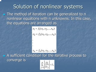
- 125. Solution of nonlinear systems Sufficient condition for convergence of this procedure is ∂f ∂f ∂g ∂g + <1 + <1 ∂x ∂y ∂x ∂y In an interval about the root that includes the initial guess This method depends on the arrangement of x and y i.e how x=f(x,y), and y=g(x,y) are written Depending on this arrangement, the method may converge or diverge
- 126. Solution of nonlinear systems The method of iteration can be generalized to n nonlinear equations with n unknowns. In this case, the equations are arranged as x1 = f1 ( x1, x2 ,..., xn ) x2 = f 2 ( x1, x2 ,..., xn ) . . . xn = f n ( x1, x2 ,..., xn ) A sufficient condition for the iterative process to converge is n ∂f i ∑ < 1, j =1 ∂x j
- 127. Newton technique of linearization Linear approximation of the function using a tangent to the curve Initial estimate x0 not too far from the root Move along the tangent to its intersection with x-axis, and take that as the next approximation Continue till x-values are sufficiently close or function value is sufficiently near to zero Newton’s algorithm is widely used because, at least in the near neighborhood of a root, it is more rapidly convergent than any of the other methods. Method is quadratically convergent, error of each step approaches a constant K times the square of the error of the previous step.
- 128. Newton technique of linearization The number of decimal places of accuracy doubles at each iteration Problem with this method is that of finding of f’(x). First derivative f’(x) can be written as ' f ( x0 ) f ( x0 ) tan θ = f ( x) = , x1 = x0 − . x0 − x1 ' f ( x0 ) We continue the calculation by computing f ( x1 ) x2 = x1 − . ' f ( x1 ) In more general form, f ( xn ) xn +1 = xn − , n = 0,1,2,... ' f ( xn )
- 129. Newton-Raphson method F(x,y)=0, G(x,y)=0 Expand the equation, using Taylor series about xn and yn F ( xn + h, yn + k ) = 0 = F ( xn , yn ) + Fx ( xn , yn )h + Fy ( xn , yn )k G ( x n + h, y n + k ) = 0 = G ( x n , y n ) + G x ( x n , y n ) h + G y ( x n , y n ) k h = xn +1 − xn , k = yn +1 − yn Solving for h and k GFy − FGY FG x − GFx h= ; k= FxG y − G x Fy FxG y − G x Fy Assume initial guess for xn,yn Compute functions, derivatives and xn,yn, h and k, Repeat procedure
- 130. Newton-Raphson method For n nonlinear equation Fi ( x1 + ∆x1, x2 + ∆x2 + ... + xn + ∆xn ) = 0 ∂Fi ∂Fi ∂Fi = Fi ( x1, x2 ,..., xn) + ∆x1 + ∆x2 + ... + ∆xn , ∂x1 ∂x2 ∂xn i = 1,2,3,..., n ∂F1 ∂F ∂F ∆x1 + 1 ∆x2 + ... + 1 ∆xn = − F1 ( x1, x2 ,..., xn) ∂x1 ∂x2 ∂xn ∂F2 ∂F ∂F ∆x1 + 2 ∆x2 + ... + 2 ∆xn = − F2 ( x1, x2 ,..., xn) ∂x1 ∂x2 ∂xn . . . ∂Fn ∂F ∂F ∆x1 + n ∆x2 + ... + n ∆xn = − Fn ( x1, x2 ,..., xn) ∂x1 ∂x2 ∂xn
- 131. Picard’s technique of linearization Nonlinear equation is linearized through: Picard’s technique of linearization Newton technique of linearization The Picard's method is one of the most commonly used scheme to solve the set of nonlinear differential equations. The Picard's method usually provide rapid convergence. A distinct advantage of the Picard's scheme is the simplicity and less computational effort per iteration than more sophisticated methods like Newton- Raphson method.
- 132. Picard’s technique of linearization The general (parabolic type) equation for flow in a two dimensional, anisotropic non-homogeneous aquifer system is given by the following equation ∂ ⎡ ∂h ⎤ ∂ ⎡ ∂h ⎤ ∂h Tx ⎥ + ⎢ ∂x ⎢Ty ⎥ =S + Q p − Rr − Rs − Q1 ∂x ⎣ ⎦ ∂y ⎣ ∂y ⎦ ∂t Using the finite difference approximation at a typical interior node, the above ground water equation reduces to Bi, j hi, j −1 + Di, j hi −1, j + Ei, j hi, j + Fi, j hi +1, j + H i, j hi, j +1 = Ri, j
- 133. Picard’s technique of linearization Where [T yi , j + T yi , j +1 ] Bi, j = − 2∆y 2 [Txi , j + Txi −1, j ] Di, j = − 2∆x 2 [Txi , j + Txi +1, j ] Fi, j = − 2∆x 2 [T yi , j + T yi , j +1 ] H i, j = − 2∆y 2
- 134. Picard’s technique of linearization Si , j Ei, j = −( Bi, j + Di, j + Fi, j + H i, j ) + ∆t Si, j h0i , j Ri, j = − (Q ) pi , j + ( R) ri , j + ( R ) si , j ∆t The Picard’s linearized form of the above equation is given by B n +1, mi, j h n +1, m +1i, j −1 + D n +1, mi, j hi −1, j + E n +1, mi, j hi, j + F n +1, mi, j hi +1, j + H n +1, mi, j hi, j +1 = R n +1, mi, j
- 135. Solution of Manning’s equation by Newton’s technique Channel flow is given by the following equation 1 1/ 2 2 / 3 Q = So AR n There is no general analytical solution to Manning’s equation for determining the flow depth, given the flow rate as the flow area A and hydraulic radius R may be complicated functions of the flow depth itself.. Newton’s technique can be iteratively used to give the numerical solution Assume at iteration j the flow depth yj is selected and the flow rate Qj is computed from above equation, using the area and hydraulic radius corresponding to yj
- 136. Manning’s equation by Newton’s technique This Qj is compared with the actual flow Q The selection of y is done, so that the error f (y j) = Qj − Q Is negligibly small The gradient of f w.r.t y is df dQ j = dy j dy j Q is a constant
- 137. Manning’s equation by Newton’s technique Assuming Manning’s n constant ⎛ df ⎞ ⎜ dy ⎟ ⎝ ⎠j 1 1 d ⎜ ⎟ = So / 2 n dy ( ) A j R2 / 3 j 1 1 / 2 ⎛ 2 AR −1 / 3 dR ⎞ 2 / 3 dA ⎟ = So ⎜ +R n ⎜ 3 dy dy ⎟ ⎝ ⎠j 1 1/ 2 2 / 3 ⎛ 2 dR 1 dA ⎞ = So A j R j ⎜ ⎜ 3R dy + A dy ⎟ ⎟ n ⎝ ⎠j ⎛ 2 dR 1 dA ⎞ = Qj⎜ ⎜ 3R dy + A dy ⎟ ⎟ ⎝ ⎠j The subscript j outside the parenthesis indicates that the contents are evaluated for y=yj
- 138. Manning’s equation by Newton’s technique Now the Newton’s method is as follows ⎛ df ⎞ 0 − f ( y) j ⎜ ⎟ = ⎜ dy ⎟ ⎝ ⎠ j y j +1 − y j f (y j) y j +1 = y j − (df / dy ) j Iterations are continued until there is no significant change in y, and this will happen when the error f(y) is very close to zero
- 139. Manning’s equation by Newton’s technique Newton’s method equation for solving Manning’s equation: 1− Q/Qj y j +1 = y j − ⎛ 2 dR 1 dA ⎞ ⎜ ⎟ ⎜ 3R dy + A dy ⎟ ⎝ ⎠j For a rectangular channel A=Bwy, R=Bwy/(Bw+2y) where Bw is the channel width, after the manipulation, the above equation can be written as 1− Q/Qj y j +1 = y j − ⎛ 5 Bw + 6 y j ⎞ ⎜ ⎟ ⎜ 3 y j ( Bw + 2 y j ) ⎟ ⎝ ⎠j
- 140. Assignments 1. Solve the following set of equations by Gauss elimination: x1 + x2 + x3 = 3 2 x1 + 3x2 + x3 = 6 x1 − x2 − x3 = −3 Is row interchange necessary for the above equations? 2. Solve the system 9 x + 4 y + z = −17, x − 2 y − 6 z = 14, x + 6 y = 4, a. Using the Gauss-Jacobi method b. Using the Gauss-Siedel method. How much faster is the convergence than in part (a).?
- 141. Assignments 3. Solve the following system by Newton’s method to obtain the solution near (2.5,0.2,1.6) x2 + y2 + z 2 = 9 xyz = 1 x + y − z2 = 0 4. Beginning with (0,0,0), use relaxation to solve the system 6 x1 − 3 x2 + x3 = 11 2 x1 + x2 − 8 x3 = −15 x1 − 7 x2 + x3 = 10
- 142. Assignments 5. Find the roots of the equation to 4 significant digits using Newton-Raphson method x − 4x +1 = 0 3 6. Solve the following simultaneous nonlinear equations using Newton-Raphson method. Use starting values x0 = 2, y0 = 0. x2 + y2 = 4 xy = 1
- 143. Numerical Differentiation and Numerical Integration Module 5 3 lectures
- 144. Contents Derivatives and integrals Integration formulas Trapezoidal rule Simpson’s rule Newton’s Coats formula Gaussian-Quadrature Multiple integrals
- 145. Derivatives Derivatives from difference tables We use the divided difference table to estimate values for derivatives. Interpolating polynomial of degree n that fits at points p0,p1,…,pn in terms of divided differences, f ( x) = Pn ( x) + error = f [ x0 ] + f [ x0 , x1 ]( x − x0 ) + f [ x0 , x1, x 2]( x − x0 )( x − x1 ) + ... + f [ x0 , x1,..., xn ] ∏( x − xi ) + error Now we should get a polynomial that approximates the derivative,f’(x), by differentiating it Pn ' ( x) = f [ x0 , x1 ] + f [ x0 , x1, x2 ][( x − x1) + ( x − x0 )] n −1 ( x − x )( x − x )...( x − x + ... + f [ x0 , x1,...xn ] ∑ 0 1 n −1 ) i =0 ( x − xi )
- 146. Derivatives continued To get the error term for the above approximation, we have to differentiate the error term for Pn(x), the error term for Pn(x): f ( n +1) (ξ ) Error = ( x − x0 )( x − x1)...( x − xn ) . (n + 1)! ξ Error of the approximation to f’(x), when x=xi, is ⎡ ⎤ ⎢ n ⎥ f ( n +1) (ξ ) Error = ⎢ ∏ ( xi − x j )⎥ , ξ in [x,x0,xn]. ⎢ j =0 ⎥ (n + 1)! ⎢ j ≠i ⎣ ⎥ ⎦ Error is not zero even when x is a tabulated value, in fact the error of the derivative is less at some x-values between the points
- 147. Derivatives continued Evenly spaced data When the data are evenly spaced, we can use a table of function differences to construct the interpolating polynomial. ( x − xi ) We use in terms of: s= h s ( s − 1) 2 s ( s − 1)( s − 2) 3 Pn ( s ) = f i + s∆f i + ∆ fi + ∆ fi 2! 3! n −1 ∆n f i + ... + ∏ ( s − j ) + error ; j =0 n! ⎡ n ⎤ f ( n +1) (ξ ) Error = ⎢ ∏ ( s − j )⎥ , ⎢ j =0 ⎥ (n + 1)! ξ in [x,x0,xn]. ⎣ ⎦
- 148. Derivatives continued The derivative of Pn(s) should approximate f’(x) d d ds Pn ( s ) = Pn ( s ) dx ds dx ⎡ ⎧ ⎫ ⎤ 1⎢ n ⎪ j −1 j −1 ⎪ ⎪ ∆ j fi ⎥ ⎪ = ⎢∆fi + ∑ ⎨ ∑ ∏ ( s − l )⎬ ⎥. h⎢ j = 2 ⎪k = 0 l = 0 ⎪ j! ⎥ ⎢ ⎪ ⎩ l ≠k ⎪ ⎭ ⎥ ⎣ ⎦ ds d ( x − xi ) 1 Where = = dx dx h h (−1) n h n ( n +1) When x=xi, s=0 Error = f (ξ ), ξ in [x1,…, xn]. n +1
- 149. Derivatives continued Simpler formulas Forward difference approximation For an estimate of f’(xi), we get 1 1 1 1 f ' ( x) = [∆f i − ∆2 f i + ∆3 fi − ... ± ∆n fi ] x = xi h 2 3 n With one term, linearly interpolating, using a polynomial of degree 1, we have (error is O(h)) ' 1 1 " f ( xi ) = [∆f i ] − hf (ξ ), h 2 With two terms, using a polynomial of degree 2, we have (error is O(h2)) 1⎡ 1 ⎤ 1 f ' ( xi ) = ∆f i − ∆2 f i ⎥ + h 2 f (3) (ξ ), h⎢ ⎣ 2 ⎦ 3
- 150. Derivatives cont… Central difference approximation Assume we use a second degree polynomial that matches the difference table at xi,xi+1 and xi+2 but evaluate it for f’(xi+1), using s=1, then 1⎡ 1 2 ⎤ f ( xi +1) = ⎢∆fi + ∆ fi ⎥ + O(h 2 ), ' h⎣ 2 ⎦ Or in terms of the f - values we can write 1⎡ 1 ⎤ f ' ( xi +1 ) = ( f i +1 − fi ) + ( fi + 2 − 2 fi +1 + fi )⎥ + error h⎢ ⎣ 2 ⎦ 1 fi + 2 − fi = + error , h 2 1 error = − h 2 f (3) (ξ ) = O(h 2 ) 6
- 151. Derivatives cont… Higher-Order Derivatives We can develop formulas for derivatives of higher order based on evenly spaced data Difference operator: ∆f ( xi ) = ∆f i = f i +1 − f i Stepping operator : Ef i = f i +1 Or : E n fi = fi + n Relation between E and ∆: E=1+ ∆ Differentiation operator: D( f ) = df / dx, D n ( f ) = d n / dx n ( f ) Let us start with fi + s = E s fi , where s = ( x − xi ) / h d d Dfi + s = f ( xi + s ) = ( E s fi ) dx dx 1 d 1 = ( E f i ) = (ln E ) E s f i s h ds h
- 152. Derivatives cont… 1 If s=0, we get D= ln(1 + ∆ ) h By expanding for ln(1+∆), we get f’i and f”i 1⎛ 1 1 1 ⎞ f i' = ⎜ ∆fi − ∆2 f i + ∆3 f i − ∆4 f i + ... ⎟, h⎝ 2 3 4 ⎠ 1 ⎛ 2 11 4 5 ⎞ f i" = ⎜ ∆ f i − ∆3 f i + ∆ fi − ∆5 f i + ... ⎟, 2⎝ 12 6 ⎠ h Divided differences Central-difference formula Extrapolation techniques Second-derivative computations Richardson extrapolations
- 153. Integration formulas The strategy for developing integration formula is similar to that for numerical differentiation Polynomial is passed through the points defined by the function Then integrate this polynomial approximation to the function. This allows to integrate a function at known values Newton-Cotes integration b b ∫ f ( x)dx = ∫ Pn ( xs )dx a a The polynomial approximation of f(x) leads to an error given as: b⎛ s ⎞ n +1 ( n +1) Error = ∫ ⎜ ⎟h f (ξ )dx ⎜ ⎟ a ⎝ n + 1⎠
- 154. Newton-Cotes integration formulas To develop the Newton-Cotes formulas, change the variable of integration from x to s. Also dx = hds For any f(x), assume a polynomial Pn(xs) of degree 1 i.e n=1 x1 x1 ∫ f ( x)dx = ∫ ( f 0 + s∆f 0 )dx x0 x0 s =1 = h ∫ ( f 0 + s∆f 0 )ds s =0 1 2⎤ s 1 = hf 0 s ]1 + h∆f 0 0 ⎥ = h( f 0 + ∆f 0 ) 2⎥ 2 ⎦0 h h = [2 f 0 + ( f1 − f 0 )] = ( f 0 + f1 ) 2 2
- 155. Newton-Cotes integration formula cont... Error in the above integration can be given as x1 s ( s − 1) 1 s2 − s Error = ∫ h f (ξ )dx = h3 f " (ξ1 ) ∫ 2 " ds x0 2 0 2 1 ⎛ s 3 s 2 ⎞⎤ 3 " = h f (ξ1 )⎜ − ⎟⎥ = − 1 h3 f " (ξ ), ⎜ 6 1 4 ⎟⎥ 12 ⎝ ⎠⎦ 0 Higher degree leads complexity
- 156. Newton-Cotes integration formula cont... The basic Newton-Cotes formula for n=1,2,3 i.e for linear, quadratic and cubic polynomial approximations respectively are given below: x1 h 1 ∫ f ( x)dx = ( f 0 + f1 ) − h3 f " (ξ ) x0 2 12 x2 h 1 5 iv ∫ f ( x)dx = ( f 0 + 4 f1 + f 2 ) − h f (ξ ), x0 3 90 x3 3h 3 5 iv ∫ f ( x)dx = ( f 0 + 3 f1 + 3 f 2 + f 3 ) − h f (ξ ). x0 8 80
- 157. Trapezoidal and Simpson’s rule Trapezoidal rule-a composite formula Approximating f(x) on (x0,x1) by a straight line Romberg integration Improve accuracy of trapezoidal rule Simpson’s rule Newton-Cotes formulas based on quadratic and cubic interpolating polynomials are Simpson’s rules 1 Quadratic- Simpson’s 3 rule 3 Cubic- Simpson’s 8 rule
- 158. Trapezoidal and Simpson’s rule cont… Trapezoidal rule-a composite formula The first of the Newton-Cotes formulas, based on approximating f(x) on (x0,x1) by a straight line, is trapezoidal rule xi +1 f ( xi ) + f ( xi +1 ) h ∫ f ( x)dx = (∆x) = ( f i + f i +1 ), xi 2 2 For [a,b] subdivided into n subintervals of size h, b n h h ∫ f ( x)dx = ∑ ( f i + f i +1 ) = ( f1 + f 2 + f 2 + f 3 + ... + f n + f n +1 ); a i =12 2 b h ∫ f ( x)dx = ( f1 + 2 f 2 + 2 f 3 + ... + 2 f n + f n +1 ). a 2
- 159. Trapezoidal and Simpson’s rule cont… f(x) x1 = a x2 x3 x4 x5 xn+1 = b x Trapezoidal Rule
- 160. Trapezoidal and Simpson’s rule cont… Trapezoidal rule-a composite formula cont… 1 3 " Local error =− h f (ξ1 ), x0 < ξ1 < x1 12 Global error 1 3 " = − h [ f (ξ1 ) + f " (ξ 2 ) + ... + f " (ξ n )], 12 If we assume that f”(x) is continuous on (a,b), there is some value of x in (a,b), say x=ξ, at which the value of the sum in above equation is equal to n.f”(ξ), since nh=b-a, the global error becomes Global error 1 3 " −(b − a ) 2 " = − h nf (ξ ) = h f (ξ ) = O(h 2 ). 12 12 The error is of 2nd order in this case
- 161. Romberg Integration We can improve the accuracy of trapezoidal rule integral by a technique that is similar to Richardson extrapolation, this technique is known as Romberg integration Trapezoidal method has an error of O(h2), we can combine two estimate of the integral that have h- values in a 2:1 ratio by 1 Better estimate=more accurate + (more 2n − 1 accurate-less accurate)
- 162. Trapezoidal and Simpson’s rule Simpson’s rule The composite Newton-Cotes formulas based on quadratic and cubic interpolating polynomials are known as Simpson’s rule 1 Quadratic- Simpson’s 3 rule The second degree Newton-Cotes formula integrates a quadratic over two intervals of equal width, h h f ( x)dx = [ f0 + 4 f1 + f 2 ]. 3 This formula has a local error of O(h5): 1 5 ( 4) Error = − h f (ξ ) 90
- 163. Trapezoidal and Simpson’s rule Quadratic- Simpson’s 1 3 rule cont… For [a,b] subdivided into n (even) subintervals of size h, h f ( x)dx = [ f (a ) + 4 f1 + 2 f 2 + 4 f 3 + 2 f 4 + ... + 4 f n −1 + f (b)]. 3 With an error of (b − a ) 4 ( 4) Error = − h f (ξ ) 180 We can see that the error is of 4 th order The denominator changes to 180, because we integrate over pairs of panels, meaning that the local rule is applied n/2 times
- 164. Trapezoidal and Simpson’s rule Cubic- Simpson’s 3 8 rule The composite rule based on fitting four points with a cubic leads to Simpson’s 3 rule 8 For n=3 from Newton’s Cotes formula we get 3h f ( x)dx = [ f0 + 3 f1 + 3 f 2 + f3 ]. 8 3 5 ( 4) Error = − h f (ξ ) 80 The local order of error is same as 1/3 rd rule, except the coefficient is larger
- 165. Trapezoidal and Simpson’s rule Cubic- Simpson’s 3 8 rule cont… To get the composite rule for [a,b] subdivided into n (n divisible by 3) subintervals of size h, 3h f ( x)dx = [ f (a ) + 3 f1 + 3 f 2 + 2 f 3 + 3 f 4 + 3 f 5 + 2 f 6 8 + ... + 2 f n −3 + 3 f n − 2 + 3 f n −1 + f (b)] With an error of (b − a ) 4 ( 4) Error = − h f (ξ ) 80
- 166. Extension of Simpson’s rule to Unequally spaced points When f(x) is a constant, a straight line, or a second degree polynomial ∆x2 ∫ f ( x)dx = w1 f1 + w2 f 2 + w3 f 3 − ∆x1 The functions f(x)=1, f(x)=x, f(x)=x2, are used to establish w1, w2, w3
- 167. Gaussian quadrature Other formulas based on predetermined evenly spaced x values Now unknowns: 3 x-values and 3 weights; total 6 unknowns For this a polynomial of degree 5 is needed to interpolate These formulas are Gaussian-quadrature formulas Applied when f(x) is explicitly known Example: a simple case of a two term formula containing four unknown parameters 1 f (t ) = af (t ) +bf (t ). ∫ −1 1 2 (b − a )t + b + a ⎛b−a⎞ x= dx = ⎜ ⎟dt If we let 2 so that ⎝ 2 ⎠ then b 1 b − a ⎛ (b − a )t + b + a ⎞ ∫ a f ( x)dx = ∫1 f ⎜ 2 − ⎝ 2 ⎟ ⎠
- 168. Multiple integrals Weighted sum of certain functional values with one variable held constant Add the weighted sum of these sums If function known at the nodes of a rectangular grid, we use these values b ⎛d ⎞ d ⎛b ⎞ ∫∫ A f ( x , y ) d A = ∫ ⎜ ∫ f ( x , y ) dy ⎟dx = ∫ ⎜ ∫ f ( x , y ) dx ⎟dy ⎜ a ⎝ c ⎟ ⎠ ⎜ c ⎝ a ⎟ ⎠ Newton-Cotes formulas are a convenient m n ∫ f ( x, y )dxdy = ∑ v j ∑ wi f ij j =1 i =1 ∆y ∆x = 3 2
- 169. Multiple integrals Double integration by numerical means reduces to a double summation of weighted function values 1 n ∫ f ( x)dx = ∑ ai f ( xi ). −1 i =1 1 1 1 n n n ∫ ∫ ∫ f ( x, y, z )dxdydz = ∑ ∑ ∑ ai a j ak f ( xi , yi , z k ). −1 −1 −1 i =1 j =1 k =1
- 170. Assignments 1. Use the Taylor series method to derive expressions for f‘(x) and f ‘‘(x) and their error terms using f-values that precede f0. ( These are called backward-difference formulas.) 2. Evaluate the following integrals by (i) Gauss method with 6 points (ii) Trapezoidal rule with 20 points (iii) Simpson’s rule with 10 points Compare the results. Is it preferable to integrate backwards or forwards? 5 1 ∫ ∫ x 3e x −1dx 2 (a) e − x dx (b) 0 0
- 171. Assignments 3. Compute the integral of f(x)=sin(x)/x between x=0 and x=1 using Simpson’s 1/3 rule with h=0.5 and then with h=0.25. from these two results, extrapolate to get a better result. What is the order of the error after the extrapolation? Compare your answer with the true answer. 4. Integrate the following over the region defined by the portion of a unit circle that lies in the first quadrant. Integrate first with respect to x holding y constant, using h=0.25. subdivide the vertical lines into four panels. ∫∫ cos( x) sin(2 y)dxdy a. Use the trapezoidal rule b. Use Simpson’s 1/3 rule
- 172. Assignments 5. Integrate with varying values of ∆x and ∆y using the trapezoidal rule in both directions, and show that the error decreases about in proportion to h2: 1 1 ∫∫ 0 0 ( x 2 + y 2 )dxdy 6. Since Simpson’s 1/3 rule is exact when f(x) is a cubic, evaluation of the following triple integral should be exact. Confirm by evaluating both numerically and analytically. 1 2 0 ∫∫ ∫ x 3 yz 2 dxdydz 0 0 −1
- 173. Numerical Solution of Ordinary Differential Equations Module 6 (6 lectures)
- 174. Contents Taylor series method Euler and modified Euler methods Rungekutta method and Multi- step method Application to higher order equations Example through open channel and pipe flow problems
- 175. Introduction Numerical solution of ordinary differential equations is an important tool for solving a number of physical real world problems which are mathematically represented in terms of ordinary differential equations. Such as spring-mass system, bending of beams, open channel flows, pipe flows etc. The most of the scientific laws are represented in terms of ordinary differential equations, so to solve such systems we need efficient tools
- 176. Introduction If the differential equation contains derivatives of nth order, its called nth order differential equation. The solution of any differential equation should be such that it satisfies the differential equation along with certain initial conditions on the function. For the nth order equation, n independent initial conditions must be specified.
- 177. Introduction These equations can be solved analytically also, but those are limited to certain special forms of equations These equations can be linear or nonlinear. When the coefficients of these equations are constants, these are linear differential equations When the coefficients itself are functions of dependent variables, these are nonlinear differential equations
- 178. Introduction Numerical methods are not limited to such standard cases, it can be used to solve any physical situations. In numerical methods we get solution as a tabulation of values of the function at various values of the independent variable and data can be fit to some functional relationship, instead of exact functional relationship as in the analytical methods. The disadvantage of this method is that we have to re- compute the entire table if the initial conditions are changed
- 179. Introduction An equation of the form dy/dx=f(x), with f(x) given and with suitable initial conditions, say y(a), also given can be integrated analytically or numerically by the methods discussed in the previous section, such as Simpson’s 1/3 rule. x y ( x) = y (a ) + ∫ f (t )dt a If f(t) cannot be integrated analytically a numerical procedure can then be employed. The more general problem is nonlinear and of the form dy/dx=f(x,y), f and y(a) given, the problem is to find y(x) for x>a
- 180. Taylor-series method Taylor series in which we expand y about the point x=x0 is ' y '' ( x0 ) 2 y ''' ( x0 ) y ( x) = y ( x0 ) + y ( x0 )( x − x0 ) + ( x − x0 ) + ( x − x0 )3 + ... 2! 3! If we assume x − x0 = h Since y( x0 ) is initial condition, first term is known ' y '' ( x0 ) 2 y ''' ( x0 ) 3 y ( x) = y ( x0 ) + y ( x0 )h + h + h + ... 2! 3! Error term of the Taylor series after the h4 term can be written as (v ) y (ξ ) 5 Error = h , 5! where 0<ξ<h
- 181. Euler and modified Euler methods If derivative is complicated, Taylor series is not comfortable to use,error is difficult to determine Euler method uses first two terms of Taylor series, choosing h small enough to truncate the series after the first derivative term, then y" (ξ )h 2 y ( x0 + h) = y ( x0 ) + y ' ( x0 ) + , 2 yn +1 = yn + hy 'n + O (h 2 ).
- 182. Euler and modified Euler methods cont… Problem is lack of accuracy, requiring an extremely small step size If we use the arithmetic mean of the slopes at the beginning and end of the interval to compute yn+1: yn ' + yn +1' yn +1 = yn + h . 2 This assumption gives us an improved estimate for y at xn+1. y’n+1 can not be evaluated till the true value of yn+1 is known
- 183. Euler and modified Euler methods Modified Euler method predicts a value of yn+1 by simple Euler relation. It then uses this value to estimate y’n+1 giving an improved estimate of yn+1 We need to re-correct yn+1 value till it makes the difference negligible y We can find out the error in the modified Euler method by comparing with the Taylor series
- 184. Euler and modified Euler methods cont… This method is called Euler predictor-corrector method '1 '' 2 y ''' (ξ ) 3 yn +1 = yn + y n h + y n h + h . 2 6 Approximating y” by forward difference, which has the error of O(h): ⎛ ⎡ ' ' ⎤ ⎞ ⎜ y ' + 1 ⎢ yn +1 − y n + O(h)⎥ h ⎟ + O(h3 ), yn +1 = yn + h⎜ n ⎜ 2⎢ ⎣ h ⎥ ⎟ ⎦ ⎠ ⎟ ⎝ ⎛ 1 1 ⎞ yn +1 = yn + h⎜ y 'n + y 'n +1 − y 'n ⎟ + O(h3 ), ⎝ 2 2 ⎠ ⎛ y 'n + y 'n +1 ⎞ yn +1 = yn + h⎜ ⎟ + O(h3 ). ⎜ 2 ⎟ ⎝ ⎠
- 185. Runge-Kutta methods Fourth and fifth order Runge-Kutta methods Increment to the y is a weighted average of two estimates of the increment which can be taken as k1 and k2. Thus for the equation dy/dx=f(x,y) yn +1 = yn + ak1 + bk 2 k1 = hf ( xn , yn ), k 2 = hf ( xn + αh, yn + βk1). We can think of the values k1 and k2 as estimates of the change in y when x advances by h, because they are the product of the change in x and a value for the slope of the curve, dy/dx.
- 186. Runge-Kutta methods cont… Uses Euler estimate of the first estimate of ∆y, the other estimate is taken with x and y stepped up by the fractions α and β of h and of the earlier estimate of ∆y, k1 Our problem is to devise a scheme of choosing the four parameters a, b,α,β. We do so by making Equations… h2 yn +1 = yn + hf ( xn , yn ) + f ' ( xn , yn ) + ... 2 An equivalent form, since df/dx=fx+fydy/dx==fx+fyf, is ⎛1 1 ⎞ yn +1 = yn + hf n + h 2 ⎜ f x + f y f ⎟ ⎝2 2 ⎠n
- 187. Runge-Kutta methods cont… Fourth order Runge-Kutta methods are most widely used and are derived in similar fashion The local error term for the 4 th order Runge-Kutta method is O(h5) ; the global error would be O(h4). Computationally more efficient than the modified Euler method, because while four evaluation of the function are required rather than two, the steps can be many fold larger for the same accuracy.
- 188. Runge-Kutta methods cont… The most commonly used set of values leads to the algorithm 1 yn +1 = yn + (k1 + 2k 2 + 2k3 + k 4 ) 6 k1 = hf ( xn , yn ), 1 1 k 2 = hf ( xn + h, yn + k1 ), 2 2 1 1 k3 = hf ( xn + h, yn + k 2 ), 2 2 k 4 = hf ( xn + h, yn + k3 ),
- 189. Multi-step methods Runge-kutta type methods are called single step method When only initial conditions are available, ability to perform the next step with a different step size Uses past values of y and y’ to construct a polynomial that approximates the derivative function, and extrapolate this into the next interval The number of past points that are used sets the degree of the polynomial and is therefore responsible for the truncation error. The order of the method is equal to the power of h in the global error term of the formula, which is also equal to one more than the degree of the polynomial.
- 190. Multi-step methods Adams method, we write the differential equation dy/dx=f(x,y) in the form dy=f(x,y)dx, and we integrate between xn and xn+1: x n +1 x n +1 ∫ dy = yn +1 − yn = ∫ f ( x, y )dx xn xn We approximate f(x,y) as a polynomial in x, deriving this by making it fit at several past points Using 3 past points, approximate polynomial is quadratic, and for 4 points the polynomial is cubic More the past points, better the accuracy, until round-off error is negligible
- 191. Multi-step methods Suppose that we fit a second degree polynomial through the last three points (xn,yn),(xn-1,yn-1) and (xn-2,yn-2), we get a quadratic approximation to the derivative function: 1 2 1 f ( x, y ) = h ( f n − 2 f n −1 + f n − 2 ) x 2 + h(3 f n − 4 f n −1 + f n − 2 ) x + f n 2 2 Now we integrate between xn and xn+1. The result is a formula for the increment in y h yn +1 − yn = (23 f n − 16 f n −1 + 5 f n − 2 ) 12
- 192. Multi-step methods We have the formula to advance y: h yn +1 = yn + [23 f n − 16 f n −1 + 5 f n − 2 ] + O(h 4 ) 12 This formula resembles the single step formulas, in that the increment to y is a weighted sum of the derivatives times the step size, but differs in that past values are used rather than estimates in the forward direction. We can reduce the error by using more past points for fitting a polynomial
- 193. Multi-step methods In fact, when the derivation is done for four points to get a cubic approximation to f(x,y), the following is obtained h yn +1 = yn + [55 f n − 59 f n −1 + 37 f n − 2 − 9 f n −3 ] + O(h5 ) 24
- 194. Multi-step methods Milne’s method first predict a value for yn+1 by extrapolating the values for the derivative, Differs from Adam’s method, as it integrates over more than one interval The required past values computed by Runge-Kutta or Taylor’s series method. In this method, the four equi-spaced starting values of y are known, at the points xn, xn-1, xn-2 and xn-3 We may apply quadrature formula to integrate as follows
- 195. Multi-step methods Milne’s method dy = f ( x, y ) dx xn+1 xn+1 xn+1 ⎛ dy ⎞ ∫ ⎜ dx ⎟dx = x∫ f ( x, y)dx = x∫ P2 ( x)dx xn−3 ⎝ ⎠ n −3 n −3 4h 28 5 v yn +1 − yn −3 = (2 f n − f n−1 + 2 f n−2 ) + h y (ξ1 ) 3 90 Where xn −3 < ξ1 < xn +1
- 196. Multi-step methods The above predictor formula can be corrected by the following xn+1 xn+1 xn+1 ⎛ dy ⎞ ∫ ⎜ dx ⎟dx = x∫ f ( x, y)dx = x∫ P2 ( x)dx xn−1 ⎝ ⎠ n −1 n −1 5 h h v yn +1,c − yn −1 = ( f n +1 + 4 f n + f n −1 ) − y (ξ 2 ) 3 90 Where xn −1 < ξ 2 < xn +1
- 197. Multi-step methods Adam-Moulton Method, more stable than and as efficient as Milne method . Adam-Moulton predictor formula: h 251 5 v yn +1 = yn + [55 f n − 59 f n −1 + 37 f n − 2 − 9 f n −3 ] + h y (ξ1 ) 24 720 Adam-Moulton corrector formula: h 19 5 v yn +1 = yn + [9 f n +1 + 19 f n − 5 f n −1 + f n − 2 ] − h y (ξ 2 ) 24 720 The efficiency of this method is about twice that of Runge-Kutta and Runge-kutta Fehlberg methods
- 198. Application to systems of equations and higher-order equations Generally any physical problems deals with a set of higher order differential equations. For example, the following equation represents a vibrating system in which a linear spring with spring constant k restores a displaced mass of weight w against a resisting force whose resistance is b times the velocity. The f(x,t) is an external forcing function acting on the mass. w d 2x dx +b + kx = f ( x, t ) g dt 2 dt
- 199. System of equations and higher-order equations Reduce to a system of simultaneous first order equations For a second order equations the initial value of the function and its derivative are known i.e the n values of the variables or its derivatives are known, where n is the order of the system. When some of the conditions are specified at the boundaries of the specified interval, we call it a boundary value problem
- 200. Systems of equations and higher-order equations By solving for second derivative, we can normally express second order equation as d 2x ⎛ dx ⎞ = f ⎜ t , x, ⎟, x(t0 ) = x0, x ' (t0 ) = x0 ' dt 2 ⎝ dt ⎠ The initial value of the function x and its derivatives are specified We convert to 1st order equation as dx = y, x(t0 ) = x0, dt
- 201. Systems of equations and higher-order equations Then we can write dy ' = f (t , x , y ), y (t0 ) = x0 dt This pair of equations is equivalent to the original 2nd order equation For even higher orders, each of the lower derivatives is defined as a new function, giving a set of n first-order equations that correspond to an nth order differential equation. For a system of higher order equations, each is similarly converted, so that a larger set of first order equations results.
- 202. Systems of equations and higher-order equations Thus the nth order differential equation ( n −1) y (n) = f ( x, y, y ,..., y ' ), y ( x0 ) = A1 , y ' ( x0 ) = A2 , . . . y ( n −1) ( x0 ) = An
- 203. Systems of equations and higher-order equations Can be converted into a system of n first-order differential equations by letting y1=y and y1' = y2 , y 2 = y3 , ' . . . yn −1 = yn , ' yn = f ( x, y1 , y2 ,..., yn ); '
- 204. Systems of equations and higher-order equations With initial conditions y1 ( x0 ) = A1 , y2 ( x0 ) = A2 , . . . yn ( x0 ) = An Now the Taylor-Series method, Euler Predictor-Corrector method, Runge-Kutta method, Runge-Kutta Fehlberg method, Adams-Moulton and Milne methods can be used to derive the various derivatives of the function
- 205. Examples of Open Channel Problems Steady flow through open channel dVs d ρVs + ( p + γz ) = 0 ds ds Where p = pressure intensity Steady, uniform flow through open channel d ( p + γz ) = 0 ds The equation describing the variation of the flow depth for any variation in the bottom elevation is given by dz dy = ( Fr2 − 1) dx dx
- 206. Examples of Open Channel Problems For gradually varied flow, variation of y with x dy S o − S f = dx 1 − Fr2 Or Gradually varied flow can be written as dy So − S f = dx 1 − (αQ 2 B) /( gA3 ) For a very wide rectangular channel, R≈y dy gB ( SoC 2 B 2 y 3 − Q 2 ) = dx C 2 ( gBy 3 − αBQ 2 )
- 207. Examples of Pipe Flow Problems Laminar flow, velocity distribution r0 − r 2 2 ⎡ d ⎤ u= 4µ ⎢− ds ( p + γz )⎥ ⎣ ⎦ Time for flow establishment in a pipe d pA + γAL sin α − τ 0πDL = (V ρ AL ) dt Surge tank water-level Oscillations, the dynamic equation is dQ gAt = ( − z − cQ Q ) dt L
- 208. Assignments 1. Use the simple Euler method to solve for y(0.1) from dy = x + y + xy y ( 0) = 1 dx With h=0.01. Repeat this exercise with the modified Euler method with h=0.025. Compare the results. 2. Determine y at x=0.2(0.2)0.6 by the Runge-Kutta technique, given that dy 1 = y (0) = 2 dx x + y
- 209. Assignments 3. Solve the following simultaneous differential equations by using (i) A fourth order Runge-Kutta method (ii) A fourth order Milne predictor-corrector algorithm dy dz = − x − yz, = − y − xz, y (0) = 0, z (0) = 1.0 dx dx For 0.5 ≥ x ≥ 0.0 4. Express the third order equation y + ty − ty − 2 y = t , y (0) = y (0) = 0, y (0) = 1, ''' '' ' '' ' a set of first order equations and solve at t =0.2,0.4,0.6 by the Runge-Kutta method (h=0.2).
- 210. Assignments 5. Find y at x=0.6, given that y '' = yy ' , y (0) = 1, y ' (0) = −1 Begin the solution by the Taylor-series method, getting y(0.1),y(0.2),y(0.3). The advance to x=0.6 employing the Adams-Moulton technique with h=0.1 on the equivalent set of first-order equations. 6. Solve the pair of simultaneous equations by the modified Euler method for t=0.2(0.2)0.6. Recorrect until reproduced to three decimals. dx dy = xy + t , x(0) = 0, = x − t , y (0) = 1, dt dt
- 211. Introduction to Finite Difference Techniques Module 7 6 lectures
- 212. Contents Types of finite difference techniques Explicit and implicit techniques Methods of solution Application of FD techniques to steady and unsteady flows in open channels
- 213. Types of FD techniques Most of the physical situation is represented by nonlinear partial differential equations for which a closed form solution is not available except in few simplified cases Several numerical methods are available for the integration of such systems. Among these methods, finite difference methods have been utilized very extensively Derivative of a function can be approximated by FD quotients.
- 214. Types of FD techniques Differential equation is converted into the difference equation Solution of difference equation is an approximate solution of the differential equation. Example: f(x) be a function of one independent variable x. assume at x0, function be f(x0) , then by using Taylor series expansion, the function f(x0+∆x) may be written as (∆x) 2 '' f ( x0 + ∆x) = f ( x0 ) + ∆xf ' ( x0 ) + f ( x0 ) + O(∆x)3 2!
- 215. Types of FD techniques f’(x0)=dy/dx at x=x0 O(∆x)3: terms of third order or higher order of ∆x Similarly f(x0- ∆x) may be expressed as ' ( ∆ x ) 2 '' f ( x0 − ∆ x ) = f ( x0 ) − ∆ xf ( x0 ) + f ( x0 ) + O ( ∆ x ) 3 2! Equation may be written as f ( x0 + ∆x) = f ( x0 ) + ∆xf ' ( x0 ) + O(∆x) 2 From this equation df f ( x0 + ∆x) − f ( x0 ) = + O(∆x) dx x = x ∆x 0i
- 216. Types of FD techniques f(x) y=f(x) B Q A x0-∆x x0 x0+∆x x Finite Difference Approximation
- 217. Types of FD techniques Similarly df f ( x0 ) − f ( x0 − ∆x) = + O(∆x) dx x = x ∆x 0i Neglecting O(∆x) terms in above equation we get Forward difference formula as given below df f ( x0 + ∆x) − f ( x0 ) = dx x = x ∆x 0i Backward difference formula as shown below df f ( x0 ) − f ( x0 − ∆x) = dx x = x ∆x 0i Both forward and backward difference approximation are first order accurate
- 218. Types of FD techniques cont… Subtracting the forward Taylor series From backward Taylor series, rearrange the terms, and divide by ∆x df f ( x0 + ∆x) − f ( x0 − ∆x) = + O(∆x) 2 dx x = x 2∆x 0i Neglecting the last term df f ( x0 + ∆x) − f ( x0 − ∆x) = dx x = x 2∆x 0i
- 219. Types of FD techniques cont… This approximation is referred to as central finite difference approximation Error term is of order O(∆x)2, known as second order accurate Central-difference approximations to derivates are more accurate than forward or backward approximations [O(h2) verses O(h)] Consider FD approximation for partial derivative
- 220. Types of FD techniques cont… Function f(x,t) has two independent variables, x and t Assume uniform grid size of ∆x and ∆t t x k+1 k t k-1 i-1 i i+1 x Finite Difference Grid Approximation
- 221. Explicit and implicit techniques There are several possibilities for approximating the partial derivatives The spatial partial derivatives replaced in terms of the variables at the known time level are referred to as the explicit finite difference The spatial partial derivatives replaced in terms of the variables at the unknown time level are called implicit finite difference k is known time level and k+1 is the unknown time level. Then FD approximation for the spatial partial derivative , ∂f/∂x, at the grid point (i,k) are as follows:
- 222. Explicit and implicit techniques Explicit finite differences Backward: f ik − f ik ∂f −1 = ∂x ∆x Forward: ∂f f ik − f ik = +1 ∂x ∆x Central: ∂f f ik 1 − f ik 1 = + − ∂x 2 ∆x
- 223. Explicit and implicit techniques Implicit finite differences ∂f f ik +1 − f ik +1 Backward: = −1 ∂x ∆x Forward: ∂f f ik +1 − f ik +1 = +1 ∂x ∆x ∂f f ik +1 − f ik +1 Central: = +1 −1 ∂x 2∆x
- 224. Explicit and implicit techniques By the known time level we mean that the values of different dependent variables are known at this time We want to compute their values at the unknown time level The known conditions may be the values specified as the initial conditions or they may have been computed during previous time step
- 225. Explicit finite difference schemes For the solution of hyperbolic partial differential equations, several explicit finite difference schemes have been proposed In the following section a number of typical schemes have been discussed which has its high relevance in hydraulic engineering Unstable scheme For any unsteady situation, we can select the following finite-difference approximations:
- 226. Explicit finite difference schemes Approximations ∂f fik 1 − f ik 1 = + − ∂x 2∆x ∂f f ik +1 − f ik = ∂t ∆t In the above f refers to dependent variables Generally the finite difference scheme is inherently unstable; i.e., computation become unstable irrespective of the size of grid spacing, so the stability check is an important part of the numerical methods.
- 227. Explicit finite difference schemes Diffusive scheme This scheme is slightly varying than the unstable scheme This method is easier to program and yields satisfactory results for typical hydraulic engineering applications. In this method the partial derivatives and other variables are approximated as follows: ∂f f ik 1 − f ik 1 ∂f f ik +1 − f * = + − = ∂x 2 ∆x ∂t ∆t
- 228. Explicit finite difference schemes where 1 k f = ( f i −1 − f ik 1 ) * + 2 These approximations are applied to the conservation and non-conservation forms of the governing equations of the physical situations.
- 229. Explicit finite difference schemes MacCormack Scheme This method is an explicit, two-step predictor-corrector scheme that is a second order accurate both in space and time and is capable of capturing the shocks without isolating them This method has been applied for analyzing one- dimensional, unsteady, open channel flows by various hydraulic engineers The general formulation for the scheme has been discussed as
- 230. Explicit finite difference schemes MacCormack Scheme cont… Two alternative formulations for this scheme are possible. In the first alternative, backward FD are used to approximate the spatial partial derivatives in the predictor part and forward FD are utilized in the corrector part. The values of the variables determined during the predictor part are used during the corrector part In the second alternative forward FDs are used in the predictor and backward FD are used in the corrector part
- 231. Explicit finite difference schemes MacCormack Scheme cont… Generally it is recommended to alternate the direction of differencing from one time step to the next The FD approximations for the first alternative of this scheme is given as follows. The predictor ∂f f i* − f ik ∂f f ik − f ik −1 = = ∂t ∆t ∂x ∆x
- 232. Explicit finite difference schemes MacCormack Scheme cont… The subscript * refers to variables computed during the predictor part The corrector ∂f f i** − f ik ∂f f i* 1 − f i* = = + ∂t ∆t ∂x ∆x the value of fi at the unknown time level k+1 is given by k +1 1 * fi = ( fi + f i** ) 2
- 233. Explicit finite difference schemes Lambda scheme In this scheme, the governing are is first transformed into λ-form and then discretize them according to the sign of the characteristic directions, thereby enforcing the correct signal direction. In an open channel flow, this allows analysis of flows having sub- and supercritical flows. This scheme was proposed by Moretti (1979) and has been used for the analysis of unsteady open channel flow by Fennema and Choudhry (1986)
- 234. Explicit finite difference schemes Lambda scheme cont… Predictor 2 f ik − 3 f ik 1 + f ik 2 − f ik 1 − f ik + fx = − − fx = + ∆x ∆x Corrector + fi* − fi* 1 − * * * − − 2 f i + 3 f i −1 − f i − 2 fx = fx = ∆x ∆x
- 235. Explicit finite difference schemes By using the above FD s and ∂f f i** − fik = ∂t ∆t and using the values of different variables computed during the predictor part, we obtain the equations for unknown variables. The values at k+1 time step may be determined from the following equations: k +1 1 * fi = ( fi + fi** ) 2
- 236. Explicit finite difference schemes Gabutti scheme This is an extension of the Lambda scheme. This allows analysis of sub and super critical flows and has been used for such analysis by Fennema and Chaudhry (1987) The general formulation for this scheme is comprised of predictor and corrector parts and the predictor part is subdivided into two parts The λ-form of the equations are used the partial derivatives are replaced as follows:
- 237. Explicit finite difference schemes Gabutti scheme cont… Taking into consideration the correct signal direction Predictor: Step1: spatial derivatives are approximated as follows: + f ik − f ik 1 − f ik 1 − f ik fx = − fx = + ∆x ∆x
- 238. Explicit finite difference schemes Gabutti scheme cont… By substituting ∂f f i** − f ik = ∂t ∆t Step2: in this part of the predictor part we use the following finite-difference approximations: + 2 f ik − 3 f ik 1 + f ik 2 − − − − 2 f ik + 3 f ik 1 − f ik 2 − − fx = fx = ∆x ∆x
- 239. Explicit finite difference schemes Gabutti scheme cont… Corrector: in this part the predicted values are used and the corresponding values of coefficients and approximate the spatial derivatives by the following finite differences: + f i* − f i* 1 − − f i* 1 − f i* fx = fx = + ∆x ∆x The values at k+1 time step may be determined from the following equations: k +1 k 1 fi = fi + ∆t ( fi* + fi** ) 2
- 240. Implicit finite difference schemes In this scheme of implicit finite difference, the spatial partial derivatives and/or the coefficients are replaced in terms of the values at the unknown time level The unknown variables are implicitly expressed in the algebraic equations, this methods are called implicit methods. Several implicit schemes have been used for the analysis of unsteady open channel flows. The schemes are discussed one by one.
- 241. Implicit finite difference schemes Preissmann Scheme This method has been widely used The advantage of this method is that the variable spatial grid may be used Steep wave fronts may be properly simulated by varying the weighting coefficient This scheme also yields an exact solution of the linearized form of the governing equations for a particular value of ∆x and ∆t.
- 242. Implicit finite difference schemes Preissmann Scheme cont… General formulation of the partial derivatives and other coefficients are approximated as follows: ∂f ( f ik +1 + f ik +1 ) − ( f ik + f ik 1 ) +1 + = ∂t 2 ∆t ∂f α ( f ik +1 − f ik +1 ) +1 (1 − α )( f ik 1 − f ik ) + = + ∂x ∆x ∆x 1 k +1 k +1 1 f = α ( fi +1 + fi ) + (1 − α )( fik 1 + fik ) + 2 2
- 243. Implicit finite difference schemes Preissmann Scheme Where α is a weighting coefficient and f refers to unknown variables and coefficients. By selecting a suitable value for α, the scheme may be made totally explicit (α=0) or implicit (α=0) The scheme is stable if 0.55< α≤1
- 244. Assignments 1. A large flat steel plate is 2 cm thick. If the initial temperature within the plate are given, as a function of the distance from one face, by the equations u = 100 x for 0 ≤ x ≤ 1 u = 100(2 − x) for 0 ≤ x ≤ 1 Find the temperatures as a function of x and t if both faces are maintained at 0 degree centigrade. The one dimensional heat flow equation is given as follows ∂u k ∂ 2u = ∂t cρ ∂x 2 Take k=0.37 cρ=0.433.
- 245. Assignments 2. Solve for the temperature at t=2.06 sec in the 2-cm thick steel slab of problem (1) if the initial temperatures are given by ⎛ πx ⎞ u ( x , 0 ) = 100 sin ⎜ ⎟ ⎝ 2 ⎠ Use the explicit method with ∆x=0.25 cm. compare to the analytical solution: − 0 . 3738 t 100 e sin( π x / 2 ) 3. Using Crank-Nicolson method, solve the following equation ∂ 2u ∂u k − cρ = f (x) ∂x 2 ∂t Solve this when f ( x ) = x ( x − 1) subject to conditions u ( 0 , t ) = 0 , u (1 , t ) = 0 , u ( x , 0 ) = 0 . Take ∆x=0.2, k=0.37 cρ=0.433. solve for five time steps.
- 246. Numerical Solution of Partial Differential Equations Module 8 6 lectures
- 247. Contents Classification of PDEs Approximation of PDEs through Finite difference method Solution methods: SOR ADI CGHS
- 248. Introduction In applied mathematics, partial differential equation is a subject of great significance These type of equations generally involves two or more independent variables that determine the behavior of the dependent variable. The partial differential equations are the representative equations in the fields of heat flow, fluid flow, electrical potential distribution, electrostatics, diffusion of matter etc.
- 249. Classification of PDEs Many physical phenomenon are a function of more than one independent variable and must be represented by a partial – differential equation, usually of second or higher order. We can write any second order equation (in two independent variable) as: ∂ 2u ∂ 2u ∂ 2u ⎛ ∂u ∂u ⎞ A +B +C ⎜ x, y , u , , ⎟ = 0 + D⎜ ∂x 2 ∂x∂y ∂y 2 ⎝ ∂x ∂y ⎟ ⎠
- 250. Classification of PDEs cont… The above partial differential equation can be classified depending on the value of B2 - 4AC, Elliptic, if B2 - 4AC<0; parabolic, if B2 - 4AC=0; hyperbolic, if B2 - 4AC>0. If A,B,C are functions of x,y,and/or u,the equation may change from one classification to another at various points in the domain For Laplace’s and Poisson’s equation, B=0, A=C=1, so these are always elliptic PDEs ∂ 2u ∂ 2u + = 0 2 2 ∂x ∂y
- 251. Classification of PDEs cont… 1D advective-dispersive transport process is represented through parabolic equation, where B=0, C=0, so B2 - 4AC=0 ∂ 2C ⎛ ∂C ∂C ⎞ Dl −⎜ +u ⎟=0 2 ⎝ ∂t ∂x ⎠ ∂x 1D wave equation is represented through hyperbolic equation, where B=0, A=1 and C=- Tg/w, so B2 - 4AC>0 ∂2 y Tg ∂ 2 y − =0 2 w ∂x 2 ∂t
- 252. FD Approximation of PDEs One method of solution is to replace the derivatives by difference quotients Difference equation is written for each node of the mesh Solving these equations gives values of the function at each node of the grid network Let h=∆x= spacing of grid work in x-direction Assume f(x) has continuous fourth derivative w.r.t x and y.
- 253. FD Approximation of PDEs When f is a function of both x and y, we get the 2nd partial derivative w.r.t x, ∂2u/ ∂x2, by holding y constant and evaluating the function at three points where x equals xn, xn+h and xn-h. the partial derivative ∂2u/ ∂y2 is similarly computed, holding x constant. To solve the Laplace equation on a region in the x- y plane, subdivide the region with equi-spaced lines parallel to x-y axes
- 254. FD Approximation of PDEs To solve Laplace equation on a xy plane, consider a region near (xi,yi), we approximate ∂ 2u ∂ 2u ∇ 2u = + =0 2 2 ∂x ∂y Replacing the derivatives by difference quotients that approximate the derivatives at the point (xi,yi), we get u ( xi +1, yi ) − 2u ( xi , yi ) + u ( xi −1, yi ) ∇ 2u ( xi , yi ) = (∆x) 2 u ( xi , yi +1 ) − 2u ( xi , yi ) + u ( xi , yi −1 ) + (∆y ) 2 =0
- 255. FD Approximation of PDEs It is convenient to use double subscript on u to indicate the x- and y- values: 2 ui +1, j − 2ui, j + ui −1, j ui, j +1 − 2ui, j + ui, j −1 ∇ ui , j = + = 0. (∆x) 2 (∆y ) 2 For the sake of simplification, it is usual to take ∆x= ∆y=h 2 ∇ ui , j = 1 u [ 2 i +1, j + ui −1, j + ui, j +1 + ui, j −1 − 4ui, j = 0. ] h We can notice that five points are involved in the above relation, known as five point star formula
- 256. FD Approximation of PDEs Linear combination of u’s is represented symbolically as below 1 ⎧ 1 ⎫ 2 ⎪ ⎪ ∇ ui , j = 1 − 4 1⎬ui, j = 0. 2⎨ h ⎪⎩ 1 ⎪⎭ This approximation has error of order O(h2),provided u is sufficiently smooth enough We can also derive nine point formula for Laplace’s equation by similar methods to get 1 ⎧1 ⎪ 4 1⎫ ⎪ ∇ 2 ui , j = 4 − 20 4⎬ui, j = 0. 2 ⎨ 6h ⎪ 1 ⎩ 4 1⎪ ⎭ In this case of approximation the error is of order O(h6), provided u is sufficiently smooth enough
- 257. Methods of solution approximation through FD at a set of grid points (xi,yi), a set of simultaneous linear equations results which needs to be solved by Iterative methods Liebmann’s Method Rearrange the FD form of Laplace’s equation to give a diagonally dominant system This system is then solved by Jacobi or Guass-Seidel iterative method The major drawback of this method is the slow convergence which is acute when there are a large system of points, because then each iteration is lengthy and more iterations are required to meet a given tolerance.
- 258. SOR method of solution S.O.R method – Accelerating Convergence Relaxation method of Southwell, is a way of attaining faster convergence in the iterative method. Relaxation is not adapted to computer solution of sets of equations Based on Southwell’s technique, the use of an overrelaxation factor can give significantly faster convergence Since we handle each equation in a standard and repetitive order, this method is called successive overrelaxation (S.O.R)
- 259. SOR method of solution cont… Applying SOR method to Laplace’s equation as given below: 1 ⎧ 1 ⎫ ⎪ ⎪ ∇ 2 ui , j = 1 − 4 1⎬ui, j = 0. 2⎨ h ⎪⎩ 1 ⎪⎭ The above equation leads to ui(+1, j + ui(−1,1) + ui(,kj)+1 + ui(,kj+1) k) k+ −1 uijk +1) = ( j 4 We now both add and subtract uij(k) on the right hand side, getting ⎡ u ( k ) + u ( k +1) + u ( k ) + u ( k +1) − 4 u ( k ) ⎤ i +1, j i −1, j i , j +1 i , j −1 ij u ijk +1) = u ijk ) + ⎢ ( ( ⎥ ⎢ 4 ⎥ ⎢ ⎣ ⎥ ⎦
- 260. SOR method of solution cont… The numerator term will be zero when final values, after convergence, are used, term in bracket called”residual”, which is “relaxed” to zero We can consider the bracketed term in the equation to be an adjustment to the old value uij(k), to give the new and improved value uij(k+1) If instead of adding the bracketed term, we add a larger value (thus “overrelaxing”), we get a faster convergence. We modify the above equation by including an overrelaxation factor ω to get the new iterating relation.
- 261. SOR method of solution cont… The new iterating relation after overrelaxation ω is as: ⎡ u ( k ) + u ( k +1) + u ( k ) + u ( k +1) − 4u ( k ) ⎤ ( k +1) uij (k ) = uij + ω ⎢ i +1, j i −1, j i, j +1 i, j −1 ij ⎥ ⎢ 4 ⎥ ⎢ ⎣ ⎥ ⎦ Maximum acceleration is obtained for some optimum value of ω which will always lie in between 1.0 to 2.0 for Laplace’s equation
- 262. ADI method of solution Coefficient matrix is sparse matrix, when an elliptical PDE is solved by FD method Especially in the 3D case, the number of nonzero coefficients is a small fraction of the total, this is called sparseness The relative sparseness increases as the number of equations increases Iterative methods are preferred for sparse matrix, until they have a tridiagonal structure
- 263. ADI method of solution Mere elimination does not preserve the sparseness until the matrix itself is tridiagonal Frequently the coefficient matrix has a band structure There is a special regularity for the nonzero elements The elimination does not introduce nonzero terms outside of the limits defined by the original bands
- 264. ADI method of solution Zeros in the gaps between the parallel lines are not preserved, though, so the tightest possible bandedness is preferred Sometimes it is possible to order the points so that a pentadiagonal matrix results The best of the band structure is tridiagonal, with corresponding economy of storage and speed of solution.
- 265. ADI method of solution cont… A method for the steady state heat equation, called the alternating- direction-implicit (A.D.I) method, results in tridiagonal matrices and is of growing popularity. A.D.I is particularly useful in 3D problems, but the method is more easily explained in two dimensions. When we use A.D.I in 2D, we write Laplace’s equation as 2 u L − 2u0 + u R u A − 2u0 + u B ∇ u= + =0 2 2 (∆x) ( ∆y ) Where the subscripts L,R,A, and B indicate nodes left, right, above, and below the central node 0. If ∆x= ∆y, we can rearrange to the iterative form
- 266. ADI method of solution Iterative form is as: u Lk +1) − 2u0k +1) + u Rk +1) = −u ( k ) + 2u0k ) − u Bk ) ( ( ( A ( ( Using above equation, we proceed through the nodes by rows, solving a set of equations (tri-diagonal) that consider the values at nodes above and below as fixed quantities that are put into the RHS of the equations After the row-wise traverse, we then do a similar set of computations but traverse the nodes column-wise: u ( k + 2) − 2u0k + 2) + u Bk + 2) = −u Lk +1) + 2u0k +1) − u Rk +1) A ( ( ( ( (
- 267. ADI method of solution This removes the bias that would be present if we use only the row-wise traverse The name ADI comes from the fact that we alternate the direction after each traverse It is implicit, because we do not get u0 values directly but only through solving a set of equations As in other iterative methods, we can accelerate convergence. We introduce an acceleration factor, ρ, by rewriting equations u0k +1) = u0k ) + ρ ⎛ u ( k ) − 2u0k ) + u Bk ) ⎞ + ρ ⎛ u Lk +1) − 2u0k +1) + u Rk +1) ⎞ ( ( ⎜ A ( ( ⎟ ⎜ ( ( ( ⎟ ⎝ ⎠ ⎝ ⎠ u0k + 2) = u0k +1) + ρ ⎛ u Lk +1) − 2u0k +1) + u Rk +1) ⎞ + ρ ⎛ u ( k + 2) − 2u0k + 2) + u Bk + 2) ⎞. ( ( ⎜ ( ( ( ⎟ ⎜ A ( ( ⎟ ⎝ ⎠ ⎝ ⎠
- 268. ADI method of solution Rearranging further to give the tri-diagonal systems, we get ( k +1) ⎛ 1 ⎞ ( ( ⎛1 ⎞ ( ⎜ + 2 ⎟u0k +1) − u Rk +1) = u ( k ) − ⎜ − 2 ⎟u0k ) + u Bk ) ( − uL +⎜ ⎟ A ⎜ρ ⎟ ρ⎝ ⎠ ⎝ ⎠ ( k + 2) ⎛ 1 ⎞ ( ⎛1 ⎞ ( ⎜ + 2 ⎟u0k + 2) − u Bk + 2) = u Lk +1) − ⎜ − 2 ⎟u0k +1) + u Rk +1) . ( ( ( − uA +⎜ ⎟ ⎜ρ ⎟ ⎝ ρ ⎠ ⎝ ⎠
- 269. CGHS method The conjugate Gradient (CG) method was originally proposed by Hestens and Stiefel (1952). The gradient method solves N x N nonsingular system of simultaneous linear equations by iteration process. There are various forms of conjugate gradient method The finite difference approximation of the ground water flow governing equation at all the I.J nodes in a rectangular flow region (J rows and I columns) will lead to a set of I.J linear equations and as many unknowns,
- 270. CGHS method The I.J equations can be written in the matrix notations as AH = Y Where A = banded coefficient matrix, H= the column vector of unknowns Y= column vector of known quantities Giving an initial guess Hi for the solution vector H, we can write as follow H i +1 = H i + di
- 271. CGHS method Where di is a direction vector, Hi is the approximation to the solution vector H at the i th iterative step. A CG method chooses di such that at each iteration the B norm of the error vector is minimized, which is defined as ei +1 =< B ei +1, ei +1> 0.5 B where ei +1 = H − H i +1 = ei − di
- 272. CGHS method In which ei+1 is the error at the (i+1)th iteration. In the above equation angle bracket denotes the Euclidean inner product, which is defined as n < x, y >= ∑ xi yi i =1 In the previous equation B is a symmetric positive definite (spd) inner product matrix. In the case of symmetric positive definite matrix A, such as that arising from the finite difference approximation of the ground water flow equation, the usual choice for the inner product matrix is B=A
- 273. CGHS method A symmetric matrix A is said to be positive definite if xTAx>0 whenever x≠0 where x is any column vector. So the resulting conjugate gradient method minimizes the A norm of the error vector (i.e. ei +1 A ). The convergence of conjugate gradient method depend upon the distribution of eigenvalues of matrix A and to a lesser extend upon the condition number [k(A)] of the matrix. The condition number of a symmetric positive definite matrix is defined as k ( A ) = λmax / λmin
- 274. CGHS method Where λmax and λmin are the largest and smallest eigenvalues of A respectively. When k(A) is large, the matrix is said to be ill-conditioned, in this case conjugate gradient method may converge slowly. The condition number may be reduced by multiplying the system by a pre-conditioning matrix K-1. Then the system of linear equation given by the equation… can be modified as K −1 A H = K −1Y
- 275. CGHS method Different conjugate methods are classified depending upon the various choices of the pre- conditioning matrix. The choice of K matrix should be such that only few calculations and not much memory storage are required in each iteration to achieve this. With a proper choice of pre-conditioning matrix, the resulting preconditioned conjugate gradient method can be quite efficient. A general algorithm for the conjugate gradient method is given as follow:
- 276. CGHS method Initialize H 0 = Arbitrary − initial − guess r0 = Y − A H 0 −1 s0 = K r0 p0 = s 0 i=0 Do while till the stopping criteria is not satisfied
- 277. CGHS method ai =< si , ri > / < A pi , pi > Cont… H i +1 = H i + ai pi ri +1 = ri − ai A pi si +1 = K −1ri +1 bi =< si +1, ri +1 > / < si , ri > p i +1= si +1 + bi pi i = i +1 End do
- 278. CGHS method Where r0 is the initial residue vector, s0 is a vector, p0 is initial conjugate direction vector, ri+1,si+1 and pi+1 are the corresponding vectors at (i+1)th iterative step, k-1 is the preconditioning matrix and A is the given coefficient matrix. This conjugate algorithm has following two theoretical properties: (a) the value {Hi}i>0 converges to the solution H within n iterations (b) the CG method minimizes H i − H for all the values of i
- 279. CGHS method There are three types of operations that are performed by the CG method: inner products, linear combination of vectors and matrix vector multiplications. The computational characteristics of these operations have an impact on the different conjugate gradient methods.
- 280. Assignments 1. The equation ∂ 2u ∂ 2u ∂u 2 2+ 2− =2 ∂x ∂y ∂x is an elliptic equation. Solve it on the unit square, subject to u=0 on the boundaries. Approximate the first derivative by a central- difference approximation. Investigate the effect of size of ∆x on the results, to determine at what size reducing it does not have further effect. 2. Write and run a program for poisson’s equation. Use it to solve ∇ 2 u = xy ( x − 2)( y − 2) On the region 0 ≤ x ≤ 2 , 0 ≤ y ≤ 2 , with u=0 on all boundaries except for y=0, where u=1.0.
- 281. Assignments 3. Repeat the exercise 2, using A.D.I method. Provide the Poisson equation as well as the boundary conditions as given in the exercise 2. 4. The system of equations given here (as an augmented matrix) can be speeded by applying over-relaxation. Make trials with varying values of the factor to find the optimum value. (In this case you will probably find this to be less than unity, meaning it is under-relaxed.) ⎡8 1 − 1 | 8 ⎤ ⎢1 − 7 2 | − 4 ⎥ ⎢ ⎥ ⎢2 1 ⎣ 9 | 12 ⎥⎦
- 282. Computation of Gradually Varied and Unsteady Open Channel Flows Module 9 6 lectures
- 283. Contents Numerical integration methods for solving Gradually varied flows Finite difference methods for Saint Venant-equations Examples
- 284. Introduction For most of the practical implications, the flow conditions in a gradually varied flow are required to calculate. These calculations are performed to determine the water surface elevations required for the planning, design, and operation of open channels so that the effects of the addition of engineering works and the channel modifications on water levels may be assessed Also steady state flow conditions are needed to specify proper initial conditions for the computation of unsteady flows
- 285. Introduction Improper initial conditions introduce false transients into the simulation, which may lead to incorrect results It is possible to use unsteady flow algorithms directly to determine the initial conditions by computing for long simulation time However, such a procedure is computationally inefficient and may not converge to the proper steady state solution if the finite-difference scheme is not consistent
- 286. Introduction Various methods to compute gradually varied flows are required to develop Methods, which are suitable for a computer solution, are adopted Traditionally there are two methods-direct and standard step methods Higher order accurate methods to numerically integrate the governing differential equation are required
- 287. Equation of gradually varied flow Consider the profile of gradually varied flow in the elementary length dx of an open channel. The total head above the datum at the upstream section is V2 H = z + d cos θ + α 2g H= total head z = vertical distance of the channel bottom above the datum d= depth of flow section θ= bottom slope angle α= energy coefficient V= mean velocity of flow through the section
- 288. Equation of gradually varied flow Differentiating dH dz dd d ⎛V2 ⎞ ⎜ ⎟ = + cos θ +α dx dx dx dx ⎜ 2 g ⎟ ⎝ ⎠ The energy slope, S f = −dH / dx The slope of the channel bottom, S0 = sin θ = −dz / dx Substituting these slopes in above equations and solving for dd/dx , dd S0 − S f = dx cos θ + αd (V 2 / 2 g ) / dd
- 289. Equation of gradually varied flow This is the general differential equation for gradually varied flow For small θ, cosθ≈1, d ≈ y, and dd/dx ≈ dy/dx, thus the above equation becomes, dy S0 − S f = dx 1 + αd (V 2 / 2 g ) / dy Since V=Q/A, and dA/dy=T, the velocity head term may be expressed as d ⎛ V 2 ⎞ αQ 2 dA−2 αQ 2 dA αQ 2T α ⎜ ⎟= =− =− dy ⎜ 2 g ⎟ 2 g dy gA3 dy gA3 ⎝ ⎠
- 290. Equation of gradually varied flow Since, Z = A3 / T The above may be written as d ⎛V2 ⎞ αQ 2 α ⎜ ⎟=− dy ⎜ 2 g ⎟ gZ 2 ⎝ ⎠ Suppose that a critical flow of discharge equal to Q occurs at the section; g Q = Zc α After substituting d ⎛V2 ⎞ Zc2 α ⎜ ⎟=− dy ⎜ 2 g ⎟ Z2 ⎝ ⎠
- 291. Equation of gradually varied flow When the Manning’s formula is used, the energy slope is 2 2 n V Sf = 2.22 R 4 / 3 When the Chezy formula is used, V2 Sf = C 2R In general form, Q2 Sf = K2
- 292. Computation of gradually varied flows The analysis of continuity, momentum, and energy equations describe the relationships among various flow variables, such as the flow depth, discharge, and flow velocity throughout a specified channel length The channel cross section, Manning n, bottom slope, and the rate of discharge are usually known for these steady- state-flow computations. The rate of change of flow depth in gradually varied flows is usually small, such that the assumption of hydrostatic pressure distribution is valid
- 293. Computation of gradually varied flows The graphical-integration method: Used to integrate dynamic equation graphically Two channel sections are chosen at x1 and x2 with corresponding depths of flow y1 and y2, then the distance along the channel floor is x2 y 2 dx x = x2 − x1 = ∫ dx = ∫ dy x1 y1 dy Assuming several values of y, and computing the values of dx/dy A curve of y against dx/dy is constructed
- 294. Computation of gradually varied flows The value of x is equal to the shaded area formed by the curve, y-axis, and the ordinates of dx/dy corresponding to y1 and y2. This area is measured and the value of x is determined. It applies to flow in prismatic as well as non-prismatic channels of any shape and slope This method is easier and straightforward to follow.
- 295. Computation of gradually varied flows Method of direct integration Gradually varied flow cannot be expressed explicitly in terms of y for all types of channel cross section Few special cases has been solved by mathematical integration
- 296. Use of numerical integration for solving gradually varied flows Total head at a channel section may be written as αV 2 H =z+ y+ 2g Where H = elevation of energy line above datum; z =elevation of the channel bottom above the datum; y = flow depth; V = mean flow velocity, and α =velocity-head coefficient The rate of variation of flow depth, y, with respect to distance x is obtained by differentiating the above equation.
- 297. Solution of gradually varied flows Consider x positive in the downstream flow direction By differentiating the above energy equation, we get the water surface profile as dy So − S f = dx 1 − (αQ 2 B ) /( gA3 ) The above equation is of first order ordinary differential equation, in which x is independent variable and y is the dependent variable.
- 298. Solution of gradually varied flows In the above differential equation for gradually varied flows, the parameters are as given below: x = distance along the channel (positive in downward direction) S0 = longitudinal slope of the channel bottom Sf = slope of the energy line B = top water surface width g = acceleration due to gravity A = flow area Q = rate of discharge
- 299. Solution of gradually varied flows The right hand of the above equation shows that it is a function of x and y, so assume this function as f(x,y), then we can write above equation as dy = f ( x, y ) dx In which, So − S f f ( x, y ) = 1 − (αQ 2 B) /( gA3 ) We can integrate above differential equation to determine the flow depth along a channel length , where f(x,y) is nonlinear function. So the numerical methods are useful for its integration.
- 300. Solution of gradually varied flows These methods yields flow depth discretely To determine the value y2 at distance x2, we proceed as follows y2 x2 ∫ dy = ∫ f ( x, y )dx y1 x1 The above integration yields.. x2 y2 = y1 + ∫ f ( x, y )dx x1
- 301. Solution of gradually varied flows We the y values along the downstream if dx is positive and upstream values if dx is negative We numerically evaluate the integral term Successive application provides the water surface profile in the desired channel length To determine x2 where the flow depth will be y2, we proceed as follows: dx = F ( x, y ) dy
- 302. Solution of gradually varied flows In which 1 − (αQ 2 B) /( gA3 ) F ( x, y ) = So − S f Integrating the above differential equation we get, y2 x2 = x1 + ∫ F ( x, y )dy y1 To compute the water surface profile, we begin the computations at a location where the flow depth for the specified discharge is known We start the computation at the downstream control section if the flow is sub-critical and proceed in the upstream direction.
- 303. Solution of gradually varied flows In supercritical flows, however, we start at an upstream control section and compute the profile in the downstream direction This is due to the fact that the flow depth is known at only control section, we proceed in either the upstream or downstream direction. In the previous sections we discussed how to compute the locations where a specified depth will occur A systematic approach is needed to develop for these computations A procedure called direct step method is discussed below
- 304. Solution of gradually varied flows Direct step method Assume the properties of the channel section are known then, z = z − S (x − x ) 2 1 0 2 1 In addition, the specific energy α1V12 2 α 2V2 E1 = y1 + E2 = y 2 + 2g 2g The slope of the energy grade line is gradually varied flow may be computed with negligible error by using the corresponding formulas for friction slopes in uniform flow.
- 305. Solution of gradually varied flows The following approximations have been used to select representative value of Sf for the channel length between section 1 and 2 Average friction slope 1 S f = ( S f1 + S f 2 ) 2 Geometric mean friction slope Sf = S f1 S f 2 2 S f1 S f 2 Harmonic mean friction slope Sf = S f1 + S f 2
- 306. Solution of gradually varied flows The friction loss may be written as 1 hf = ( S f1 + S f 2 )( x2 − x1) 2 From the energy equation we can write, 1 z1 + E1 = z 2 + E 2 + ( S f1 + S f 2 )( x 2 − x1 ) 2 Writing in terms of bed slope E2 − E1 x2 = x1 + 1 S o − ( S f1 + S f 2 ) 2 Now from the above equation, the location of section 2 is known.
- 307. Solution of gradually varied flows This is now used as the starting value for the next step Then by successively increasing or decreasing the flow depth and determining where these depths will occur, the water surface profile in the desired channel length may be computed The direction of computations is automatically taken care of if proper sign is used for the numerator and denominator
- 308. Solution of gradually varied flows The disadvantages of this method are 1. The flow depth is not computed at predetermined locations. Therefore, interpolations may become necessary, if the flow depths are required at specified locations. Similarly, the cross-sectional information has to be estimated if such information is available only at the given locations. This may not yield accurate results 2. Needs additional effort 3. It is cumbersome to apply to non-prismatic channels
- 309. Solution of gradually varied flows Standard step method When we require to determine the depth at specified locations or when the channel cross sections are available only at some specified locations, the direct step method is not suitable enough to apply and in these cases standard step method is applied In this method the following steps are followed : Total head at section 1 α1V12 H 1 = z1 + y1 + 2g
- 310. Solution of gradually varied flows Total head at section 2 H 2 = H1 − h f Including the expression for friction loss hf 1 H 2 = H1 − ( S f1 + S f 2 )( x 2 − x1 ) 2 Substituting the total head at 2 in terms of different heads, we obtain α 2Q 2 1 1 y2 + + S f 2 ( x2 − x1 ) + z2 − H1 + S f1 ( x2 − x1 ) = 0 2 2 2 2 gA2
- 311. Solution of gradually varied flows In the above equation. A2 and Sf2 are functions of y2, and all other quantities are either known or already have been calculated at section 1. The flow depth y2 is then determined by solving the following nonlinear algebraic equation: α 2Q 2 1 1 F ( y2 ) = y2 + + S f 2 ( x 2 − x1 ) + z 2 − H 1 + S f1 ( x 2 − x1 ) = 0 2 2 2 2 gA2 The above equation is solved for y2 by a trial and error procedure or by using the Newton or Bisection methods
- 312. Solution of gradually varied flows Here the Newton method is discussed. For this method we need an expression for dF/dy2 dF α 2Q 2 dA2 1 d ⎛ Q 2n2 ⎜ ⎞ ⎟ =1− + ( x 2 − x1 ) dy 2 3 gA2 dy 2 2 dy 2 ⎜ C o A2 R 4 / 3 ⎜ 2 2 ⎟ ⎟ ⎝ 2 ⎠ The last term of the above equations can be evaluated as ⎛ Q 2n 2 ⎞ 2 2 2 2 d ⎜ ⎟ = − 2Q n dA2 − 4 Q n dR2 dy2 ⎜ 2 2 4/3 ⎟ ⎜ Co A2 R ⎟ Co A2 R 4 / 3 dy2 3 Co A2 R 7 / 3 dy2 2 2 2 2 ⎝ 2 ⎠ 2 2 − 2Q 2 n 2 dA2 4 Q 2 n 2 1 dR2 = − Co A2 R2 / 3 dy2 3 Co A2 R2 / 3 R2 dy2 2 2 4 2 2 4 ⎛ S ⎞ = −2⎜ S f B2 + 2 f 2 dR2 ⎟ ⎜ 2 A 3 R2 dy2 ⎟ ⎝ 2 ⎠
- 313. Solution of gradually varied flows Here dA2/dy2 is replaced by B2 in the above equation and substituting for this expression dF α 2 Q 2 B2 ⎛ B2 2 S f 2 dR 2 ⎞ =1− − ( x 2 − x1 )⎜ S f 2 + ⎟ dy 2 gA2 3 ⎜ A2 3 R2 dy 2 ⎟ ⎝ ⎠ By using y=y1, dy/dx=f(x1,y1) , then the flow depth y* , can be computed from the equation 2 y * = y1 + f ( x1 , y1 )( x 2 − x1 ) 2 During subsequent step, however may be y* 2 determined by extrapolating the change in flow depth computed during the preceding step.
- 314. Solution of gradually varied flows A better estimate for y2 can be computed from the equation * F ( y2 ) y2 = y* − 2 [dF / dy2 ]* If y2 − y* 2 is less than a specified tolerance, ε, then y* 2 is the flow depth y2, at section 2; otherwise, set y* = y2 2 and repeat the steps until a solution is obtained
- 315. Solution of gradually varied flows Integration of differential equation For the computation of the water surface profile by integrating the differential equation, the integration has to be done numerically, since f(x,y) is a nonlinear function Different numerical methods have been developed to solve such nonlinear system efficiently The numerical methods that are in use to evaluate the integral term can be divided into following categories: 1. Single-step methods 2. Predictor-corrector methods
- 316. Solution of gradually varied flows The single step method is similar to direct step method and standard step method The unknown depths are expressed in terms of a function f(x,y), at a neighboring point where the flow depth is either initially known or calculated during the previous step In the predictor-corrector method the value of the unknown is first predicted from the previous step This predicted value is then refined through iterative process during the corrector part till the solution is reached by the convergence criteria
- 317. Solution of gradually varied flows Single-step methods Euler method Modified Euler method Improved Euler method Fourth-order Runge-Kutta method 1. Euler method: In this method the rate of variation of y with respect to x at distance xi can be estimated as ' dy yi = = f ( xi , yi ) dx i
- 318. Solution of gradually varied flows The rate of change of depth of flow in a gradually varied flow is given as below S o − S fi f ( xi , y i ) = 1 − (α Q 2 Bi ) /( gAi3 ) All the variables are known in the right hand side, so derivative of y with respect to x can be obtained Assuming that this variation is constant in the interval xi to xi+1, then the flow depth at xi+1 can be computed from the equation yi +1 = yi + f ( xi , yi )( xi +1 − xi )
- 319. Solution of gradually varied flows cont.. 2. Modified Euler method We may also improve the accuracy of the Euler method by using the slope of the curve y = y (x) at x = x and i +1 / 2 1 y = yi +1/ 2 , in which xi+1/ 2 = (xi + xi+1 ) and yi +1/ 2 = yi + 1 yi' ∆x . 2 2 Let us call this slope yi' +1/ 2 . Then yi +1 = yi + yi' +1/ 2 ∆x or yi +1 = yi + f ( xi +1/ 2 , yi +1/ 2 )∆x This method, called the modified Euler method, is second- order accurate.
- 320. Solution of gradually varied flows cont.. 3. Improved Euler method Let us call the flow depth at xi +1 obtained by using Euler method as y * i.e., i +1 * yi +1 = yi + yi' ∆x By using this value, we can compute the slope of the curve ( y = y (x) at x = xi +1 , i.e., yi' +1 = f xi +1 , yi*+1 . Let us ) use the average value of the slopes of the curve at xi and xi +1 . Then we can determine the value of yi +1 from the equation yi +1 = yi + 2 ( 1 ' ) yi + yi' +1 ∆x . This equation may be yi +1 = yi + 1 [ ] f ( xi , yi ) + f ( xi +1 , yi*+1 ) ∆x written as 2 . This method called the improved Euler method, is second order accurate.
- 321. Solution of gradually varied flows cont.. 4. Fourth-order Runge Kutta Method k1 = f ( xi , yi ) 1 1 k 2 = f ( xi + ∆x, yi + k1∆x) 2 2 1 1 k3 = f ( xi + ∆x, yi + k 2 ∆x) 2 2 k 4 = f ( xi + ∆x, yi + k3∆x) 1 yi +1 = yi + (k1 + 2k 2 + 2k3 + k 4 )∆x 6
- 322. Solution of gradually varied flows cont.. Predictor-corrector methods In this method we predict the unknown flow depth first, correct this predicted value, and then re-correct this corrected value. This iteration is continued till the desired accuracy is met. In the predictor part, let us use the Euler method to predict the value of yi+1, I.e yi(+1 = yi + f ( xi , yi )∆x 0) we may correct using the following equation 1 yi +1 = yi + [ f ( xi , yi ) + f ( xi +1, yi(+1 )]∆x (1) 0) 2
- 323. Solution of gradually varied flows cont.. Now we may re-correct y again to obtain a better value: 1 yi(+1 = yi + 2) [ f ( xi , yi ) + f ( xi +1, yi(1) )]∆x +1 2 Thus the j th iteration is 1 j− yi(+1 = yi + j) [ f ( xi , yi ) + f ( xi +1, yi(+1 1) )]∆x 2 Iteration until j− yi(+1 − yi(+1 1) ≤ ε j) , where ε = specified tolerance
- 324. Saint-Venant equations 1D gradually varied unsteady flow in an open channel is given by Saint-Venant equations ∂v ∂y ∂y a + vw +w =0 ∂x ∂x ∂t ∂v ∂y ∂v v +g + = g ( So − S f ) ∂x ∂x ∂t X - distance along the channel, t - time, v- average velocity, y - depth of flow, a- cross sectional area, w - top width, So- bed slope, Sf - friction slope
- 325. Saint Venant equations Friction slope n 2v 2 Sf = r4 / 3 r - hydraulic radius, n-Manning’s roughness coefficient Two nonlinear equations in two unknowns v and y and two dependent variables x and t These two equations are a set of hyperbolic partial differential equations
- 326. Saint-Venant equations Multiplying 1st equation by ± g / aw and adding it to 2nd equation yields ⎡∂ ∂ ⎤ 1⎡∂ ∂⎤ ⎢ ∂t + (v ± c ) ∂x ⎥ v ± c ⎢ ∂t + (v ± c ) ∂x ⎥ y = g (S o − S f ) ⎣ ⎦ ⎣ ⎦ The above equation is a pair of equations along characteristics given by dx = g (S o − S f ) dv g dy =v±c ± dt dt c dt Based on the equations used, methods are classified as characteristics methods and direct methods.
- 327. FD methods for Saint Venant equations The governing equation in the conservation form may be written in matrix form as U t + Fx + S = 0 In which ⎛a ⎞ ⎛ va ⎞ ⎛0 ⎞ =⎜ ⎟ U ⎜ ⎟ F =⎜ 2 ⎟ S= ⎜ ⎟ ⎜ v a + gay ⎟ ⎜ − ga ( s0 − s f ) ⎟ ⎝ va ⎠ ⎝ ⎠ ⎝ ⎠ General formulation ∂f ( fin +1 + fin +1) − ( f in + fin 1 ) +1 + = ∂t ∆t
- 328. FD methods for Saint Venant equations Continued… n +1 n +1 n n ∂f α ( f i +1 + f i ) (1 − α )( f i +1 + f i ) = + ∂x ∆x ∆x 1 1 f = α ( f in +1 + fin +1 ) + (1 − α )( f in 1 + f in ) +1 + 2 2 U in +1 + U in +1 = 2 +1 ∆t ∆x [ α ( Fin +1 − Fin +1) + (1 − α )( Fin 1 − Fin ) +1 + ] [ + ∆t α ( Sin +1 + Sin +1 ) + (1 − α )( Sin 1 + Sin ) +1 + ] = U in + U in 1 +
- 329. FD methods for Saint Venant equations Boundary conditions: yin ++1 = yresd 1 ,j Downstream boundary: Left boundary y=yu= uniform flow depth v=vu= uniform velocity Right boundary y=yc= Critical flow depth v=vc= Critical velocity
- 330. FD methods for Saint Venant equations Stability: unconditionally stable provided α>0.5, i.e., the flow variables are weighted toward the n+1 time level. Unconditional stability means that there is no restriction on the size of ∆x and ∆t for stability
- 331. Solution procedure The expansion of the equation… ain +1 + ain +1 + 2 +1 ∆t ∆x {[ ] [ α (va)i +1 − (va)i +1 + (1 − α ) (va)i +1 − (va)i n +1 n n n ]} = ain + ain 1 + (va)i +1 + (va)i +1 + 2 n n +1 ∆t ∆x {[ α (v 2 a + gay )i +1 − (v 2 a + gay )i +1 n +1 n ]} {[ − ga∆t α ( s0 − s f )i +1 + ( s0 − s f )i +1 n +1 n ]} = ga∆t {1 − α )[( s ( 0 n n − s f )i +1 + ( s0 − s f )i ]} + (va)i + (va)i +1 − (1 − α ) 2 n n ∆t 2 ∆x { (v a + gay )i +1 − (v 2 a + gay )i n n } The above set of nonlinear algebraic equations can be solved by Newton-Raphson method
- 332. Assignments 1. Prove the following equation describes the gradually varied flow in a channel having variable cross section along its length: ( ) dy SO − S f + V / gA ∂A / ∂x = 2 dx ( ) 1 − BV 2 / ( gA) 2. Develop computer programs to compute the water- surface profile in a trapezoidal channel having a free overfall at the downstream end. To compute the profile, use the following methods: (i) Euler method (ii) Modified Euler method (iii) Fourth-order Runge-Kutta method
- 333. Assignments 3. Using method of characteristics, write a computer program to solve 1D gradually varied unsteady flow in an open channel as given by Saint-Venant equations, assuming initial and boundary conditions.
- 334. Solution of Pipe Transients and Pipe Network Problems Module 10 6 Lectures
- 335. Contents Basic equation of transients Method of characteristics for its solution Complex boundary condition Pipe network problems Node based and Loop based models Solution through Newton and Picard techniques
- 336. Basic equations of transients The flow and pressures in a water distribution system do not remain constant but fluctuate throughout the day Two time scales on which these fluctuations occur 1. daily cycles 2. transient fluctuations
- 337. Basic equations of transients Continuity equation: applying the law of conservation of mass to the control volume (x1 and x2) x2 ∂ ∫ ∂t ( ρA)dx +( ρAV ) x1 2 − ( ρAV )1 = 0 By dividing throughout by ∆x as it approach zero, the above equation can be written as ∂ ∂ ( ρA) + ( ρAV ) = 0 ∂t ∂x Expanding and rearranging various terms, using expressions for total derivatives, we obtain 1 dρ 1 dA ∂V + + =0 ρ dt A dt ∂x
- 338. Basic equations of transients Now we define the bulk modulus of elasticity, K, of a fluid as K= dp dρ ρ This can be written as dρ = ρ dp dt K dt Area of pipe, A = πR , where R is the radius of the 2 pipe. Hence dA / dt = 2πRdR / dt. In terms of strain this may be written as dA = 2 A dε dt dt dε D dp Now using hoop stress, we obtain = dt 2eE dt
- 339. Basic equations of transients Following the above equations one can write, 1 dA D dp = A dt eE dt Substituting these equations into continuity equation and simplifying the equation yields ∂V 1 ⎡ 1 ⎤ dp + ⎢1 + eE / DK ⎥ dt = 0 ∂x K⎣ ⎦ K/ρ a2 = Let us define , where a is wave speed 1 + ( DK ) / eE with which pressure waves travel back and forth. Substituting this expression we get the following continuity equation ∂p ∂p ∂V +V + ρa 2 =0 ∂t ∂x ∂x
- 340. Method of characteristics The dynamic and continuity equations for flow through a pipe line is given by ∂Q ∂H f L1 = + gA + QQ =0 ∂t ∂x 2 DA ∂Q ∂H L2 = a 2 + gA =0 ∂x ∂t Where Q=discharge through the pipe H=piezometric head A=area of the pipe g=acceleration due to gravity a=velocity of the wave D=diameter of the pipe x=distance along the pipe t=time
- 341. Method of characteristics These equations can be written in terms of velocity 1 ∂v ∂H f L1 = + + vv = 0 g ∂t ∂x 2 Dg ∂H a 2 ∂v L2 = + =0 ∂t g ∂x Where, k a= e[1 + (kD / ρE )]
- 342. Method of characteristics Where k=bulk modulus of elasticity ρ=density of fluid E=Young’s modulus of elasticity of the material Taking a linear combination of L1 and λL2, leads to ⎛ ∂Q ∂Q ⎞ ⎛ ∂H 1 ∂H ⎞ f ⎜ + λa 2 ⎟ + λgA⎜ + ⎟+ QQ =0 ⎝ ∂t ∂x ⎠ ⎝ ∂T λ ∂x ⎠ 2 DA Assume H=H(x,t);Q=Q(x,t)
- 343. Method of characteristics Writing total derivatives , dQ ∂Q ∂Q dx dH ∂H ∂H dx = + = + dt ∂t ∂x dt dt ∂t ∂x dt Defining the unknown multiplier λ as 1 dx 1 = = λa 2 λ=± λ dt a Finally we get dx dQ gA dH f = ±a ± + QQ =0 dt dt a dt 2 DA The above two equations are called characteristic equations and 2nd among them is condition along the characteristics
- 344. Method of characteristics Figure… t P Negative characteristic Positive characteristic line line A C B x Characteristic lines Constant head reservoir at x=0, at x=L, valve is instantaneously closed. Pressure wave travels in the upstream direction.
- 345. Complex boundary condition We may develop the boundary conditions by solving the positive or negative characteristic equations simultaneous with the condition imposed by the boundary. This condition may be in the form of specifying head, discharge or a relationship between the head and discharge Example: head is constant in the case of a constant level reservoir, flow is always zero at the dead end and the flow through an orifice is related to the head loss through the orifice.
- 346. Complex boundary condition Constant-level upstream reservoir In this case it is assume that the water level in the reservoir or tank remains at the same level independent of the flow conditions in the pipeline This is true for the large reservoir volume If the pipe at the upstream end of the pipeline is 1, then H P1,1 = H ru where H ru is the elevation of the water level in the reservoir above the datum. At the upstream end, we get the negative characteristic equation, QP1,1 = Cn + Ca H ru
- 347. Complex boundary condition Constant-level downstream reservoir In this case, the head at the last node of pipe i will always be equal to the height of the water level in the tank above the datum, Hrd: H Pi , n +1 = H rd At the downstream end, we have the positive characteristic equation linking the boundary node to the rest of the pipeline. We can write QPi, n +1 = Cp − Ca H rd
- 348. Complex boundary condition Dead end At a dead end located at the end of pipe i, the discharge is always zero: Q Pi , n +1 = 0 At the last node of pipe i, we have the positive characteristics equation. We get Cp H Pi , n +1 = Ca
- 349. Complex boundary condition Downstream valve In the previous boundaries, either the head or discharge was specified, However for a valve we specify a relationship between the head losses through the valve and the discharge Denoting the steady-state values by subscript 0, the discharge through a valve is given by the following equation: Q0 = C d Av 0 2gH 0
- 350. Complex boundary condition Where Cd=coefficient of discharge Av0=area of the valve opening H0=the drop in head Q0= a discharge By assuming that a similar relationship is valid for the transient state conditions, we get Q Pi , n +1 = (C d Av ) P 2 gH Pi , n +1 Where subscript P denotes values of Q and H at the end of a computational time interval
- 351. Complex boundary condition From the above two equations we can write 2 2 H Pi, n +1 QPi, n +1 = (Q0τ ) H0 Where the effective valve opening is τ = (C d Av ) P /(C d Av ) 0 For the last section on pipe i, we have the positive characteristic equation 2 QPi, n +1 + CvQPi, n +1 − C p Cv = 0
- 352. Complex boundary condition Where Cv = (τQ0 ) 2 /(Ca H 0 ) Solving for QPi,n+1 and neglecting the negative sign with the radical term, we get 2 Q Pi , n +1 = 0.5( −C v + C v + 4C p C v )
- 353. Pipe network problems The network designing is largely empirical. The main must be laid in every street along which there are properties requiring a supply. Mains most frequently used for this are 100 or 150mm diameter The nodes are points of junction of mains or where a main changes diameter. The demands along each main have to be estimated and are then apportioned to the nodes at each end in a ratio which approximated
- 354. Pipe network problems There are a number of limitations and difficulties with respect to computer analysis of network flows , which are mentioned below: 1. The limitation with respect to the number of mains it is economic to analyze means that mains of 150 mm diameter and less are usually not included in the analysis of large systems, so their flow capacity is ignored 2. It is excessively time consuming to work out the nodal demands for a large system
- 355. Pipe network problems 1. The nodal demands are estimates and may not represent actual demands 2. Losses, which commonly range from 25% to 35% of the total supply, have to be apportioned to the nodal demands in some arbitrary fashion. 3. No diversification factor can be applied to the peak hourly demands representing reduced peaking on the larger mains since the total nodal demands must equal the input to the system 4. The friction coefficients have to be estimated. 5. No account is taken of the influence of pressure at a node on the demand at that node, I.e under high or low pressure the demand is assumed to be constant.
- 356. Governing Equation for Network Analysis Every network has to satisfy the following equations: 1. Node continuity equations – the node continuity equations state that the algebraic sum of all the flows entering and leaving a node is zero. j = 1,..., NJ ∑ Q( p) + ∑ Q( p) + C ( j ) = 0, pε { j} pε { j} Where NJ is the number of nodes, Q(p) is the flow in element p (m3/s), C(j) is the consumption at node j (m3/s), pε { j} refers to the set of elements connected to node j.
- 357. Network Analysis 2. Energy conservation equations – the energy conservation equations state that the energy loss along a path equals the difference in head at the starting node and end node of the path. ∑ (± )h( p) + ∑ (± )h( p) − [H (s(l )) − H (e(l ))] = 0 l = 1,..., NL + NPATH pε {l} pε {l} Where h(p) is the head loss in element p(m), s(l) is the starting node of path l, e(l) is the end of path 1, NL is the number of loops, and NPATH is the number of paths other than loops and pε {l} refers to the pipes belonging to path l. loop is a special case of path, wherein, the starting node and end node are the same, making the head loss around a loop zero, that is, ∑ (± )h( p) + ∑ (± )h( p) = 0
- 358. Network Analysis 3. Element characteristics – the equations defining the element characteristics relate the flow through the element to the head loss in the element. For a pipe element, h(p) is given by, h( p ) = R( p )Q( p ) e Where R(p) is the resistance of pipe p and e is the exponent in the head loss equation. If Hazen-Williams equation is used, where e=1.852 10.78 L( p ) R( p) = D( p ) 4.87 CHW ( p )1.852 Where L(p) is the length of pipe p(m), D(p) is the diameter of pipe p(m), and CHW (p) is the Hazen-Williams coefficient for pipe p.
- 359. Network Analysis For a pump element, h(p) is negative as head is gained in the element. The characteristics of the pump element are defined by the head-discharge relation of the pump. This relationship may be expressed by a polynomial or in an alternate form. In this study, the following equation is used. ⎡ ⎡ Q( p) ⎤ C 3( m ) ⎤ h( p ) = − HR(m) ⎢C1(m) − C 2(m).⎢ ⎥ ⎢ ⎣ QR(m) ⎥ ⎦ ⎥ ⎣ ⎦ Where HR(m) is the rated head of the m-th pump (m), QR(m) is the rated discharge of m-th pump (m3/s), C1(m), C2(m) and C3(m) are empirical constants for the m-th pump obtained from the pump charateristics. Here p refers to the element corresponding to the m-th pump. If the actual pump characteristics are available, the constants C1, C2, C3 may be evaluated. C1 is determined from the shutoff head as HO(m) C1(m) = HR(m)
- 360. Network Analysis Where HO(m) is the shutoff head of the m-th pump. As h(p)=-HR(m) for rated flow, C1(m) − C 2(m) = 1 From which C2(m)is determined. C3 (m) is obtained by fitting the equation to the actual pump characteristics. For a pipe element, (1 / e ) ⎡ h( p ) ⎤ H (i ) − H ( j ) Q( p) = ⎢ = ⎣ R( p) ⎥⎦ R( p ) (1/ e ) H (i ) − H ( j ) (1−1 / e ) For Hazen-Williams equation, the above equation becomes H (i ) − H ( j ) Q( p) = 0.46 R ( p ) 0.54 H (i ) − H ( j )
- 361. Network Analysis Similarly for a pump element 1 ⎡ 1 ⎡ H ( j ) − H (i ) ⎤ ⎤ C 3( m ) Q( p ) = (± )QR(m) ⎢ ⎢C1(m) ± HR(m) ⎥ ⎥ ⎣ C 2( m ) ⎣ ⎦⎦ Where outside the parenthesis, + sign is used if flow is towards node j and –sign is used if flow is away from node j and, inside the parenthesis, the + sign is used, if i is the node downstream of the pump and the – sign is used if j is the node downstream of the pump.
- 362. Network Analysis The network analysis problem reduces to one of solving a set of non- linear algebraic equations. Three types of formulation are used – the nodal, the path and the node and path formulation. Each formulation and method of analysis has its own advantages and limitations. In general path formulation with Newton-Raphson method gives the fastest convergence with minimum computer storage requirements. The node formulation is conceptually simple with a very convenient data base, but it has not been favoured earlier, because in conjunction with Newton-Raphson method, the convergence to the final solution was found to depend critically on the quality of the initial guess solution. The node and path formulation can have a self starting procedure without the need for a guess solution, but this formulation needs the maximum computer storage.
- 363. Node based models The node (H) equations The number of equations to be solved can be reduced from L+J-1 to J by combining the energy equation for each pipe with continuity equation. The head loss equation for a single pipe can be written as h = KQ n nij H i − H j = K ij Qij sgn Qij Where Hi=head at i th node, L Kij= head loss coefficient for pipe from node i to node j Qij= flow in pipe from node i to node j, L3/t nij=exponent in head loss equation for pipe from i-j
- 364. Node based models The double subscript shows the nodes that are connect by a pipe Since the head loss is positive in the direction of flow, sgn Qij=sgn (Hi-Hj), and we solve for Q as 1 / nij Qij = sgn( H i − H j )( H i − H j / K ij ) The continuity equation at node I can be written as mi ∑ Qki = U i k =1 Where Qki=flow into node i from node k, L3/T Ui=consumptive use at node i, L3/T mi=number of pipes connected to node i.
- 365. Node based models Combining energy and continuity equations for each flow in the continuity equation gives 1 / nki mi ⎛ H k − Hi ⎞ ∑ sgn( H k − H i )⎜ ⎟ = Ui k =1 ⎜ K ki ⎟ ⎝ ⎠ The above is a node H equation, there is one such equation for each node, and one unknown Hi for each equation These equations are all nonlinear The node (H) equations are very convenient for systems containing pressure controlled devices I.e. check valves, pressure reducing valves, since it is easy to fix the pressure at the downstream end of such a valve and reduce the value if the upstream pressure is not sufficient to maintain downstream pressure
- 366. Loop based models The Loop (∆Q) equations One approach is to setting up looped system problems is to write the energy equations in such a way that, for an initial solution, the continuity will be satisfied Then correct the flow in each loop in such a way that the continuity equations are not violated. This is done by adding a correction to the flow to every pipe in the loop . If there is negligibly small head loss, flow is added around the loop, if there is large loss, flow is reduced Thus the problem turns into finding the correction factor ∆Q such that each loop energy equation is satisfied
- 367. Loop based models The loop energy equations may be written ml F (∆Q) = ∑ K i [sgn(Qii + ∆Ql )] Qii + ∆Ql n = dhl (l=1,2,…,L) i =1 Where Qii = initial estimate of the flow in i th pipe, L3/T ∆Ql = correction to flow in l th loop, L3/T ml = number of pipes in l th loop L = number of loops
- 368. Loop based models The Qi terms are fixed for each pipe and do not change from one iteration to the next. The ∆Q terms refer to the loop in which the pipe falls The flow in a pipe is therefore Qi + ∆Q for a pipe that lies in only one loop. For a pipe that lies in several loops (say ,a b, and c) the flow might be Qi + ∆Qa − ∆Qb + ∆Qc
- 369. Loop based models The negative sign in front of b term is included merely to illustrate that a given pipe may be situated in positive direction in one loop and in negative direction in another loop. When the loop approach is used, a total of L equations are required as there are l unknowns, one for each loop
- 370. Solution of pipe network problems through Newton-Raphson method Newton-Raphson method is applicable for the problems that can be expressed as F(x)=0, where the solution is the value of x that will force F to be zero The derivative of F can be a expressed by dF F ( x + ∆x) − F ( x) = dx ∆x Given an initial estimate of x, the solution to the problem is the value of x+∆x that forces F to 0. Setting F(x+∆x) to zero and solving for ∆x gives F ( x) ∆x = − F ' ( x)
- 371. Solution of pipe network problems through Newton-Raphson method New value of x+∆x becomes x for the next iteration. This process is continued until F is sufficiently close to zero For a pipe network problem, this method can be applied to the N-1=k, H-equations The head (H) equations for each node (1 through k), it is possible to write as: 1 / nij ⎛ H −H ⎞ [ ] mi ⎜ j i ⎟ F ( H i ) = ∑ sgn( H j − H i ) ⎜ − Ui = 0 (i = 1,2,..., K ) ⎟ j =1 ⎜ K ji ⎟ ⎝ ⎠ Where mi= number of pipes connected to node I Ui= consumptive use at node i, L3/T F(i) and F(i+1) is the value of F at ith and (i+1)th iteration, then dF = F (i + 1) − F (i )
- 372. Solution of pipe network problems through Newton-Raphson method This change can also be approximated by total derivative ∂F ∂F ∂F dF = ∆H1 + ∆H 2 + ... + ∆H k ∂H1 ∂H 2 ∂H k Where ∆H= change in H between the ith and (i+1)th iterations, L Finding the values of ∆H which forces F(i+1)=0. Setting above two equations equal, results in a system of k linear equations with k unknowns (∆H) which can be solved by the any linear methods
- 373. Solution of pipe network problems through Newton-Raphson method Initial guess for H Calculate partial derivatives of each F with respect to each H Solving the resulting system of linear equations to find H, and repeating until all of the F’s are sufficiently close to 0 The derivative of the terms in the previous equation is given by 1 / nij ⎛ H −H ⎞ d [ ( )] ⎜ i sgn H i − H j ⎜ j ⎟ = −1 (H i − H j )(1 / n )−1 (nij )(Kij )1 / n ij dH j K ij ⎟ ⎜ ⎟ ij ⎝ ⎠ 1 / nij and ⎛ H −H ⎞ d [ ( )] ⎜ i sgn H i − H j ⎜ j ⎟ = 1 (H i − H j )(1 / n )−1 (nij )(Kij )1 / n ij dH i K ij ⎟ ⎜ ⎟ ij ⎝ ⎠
- 374. Solution of pipe network problems through Hardy-Cross method The linear theory method and the Newton-Raphson method can converge to the correct solution rapidly Manual solution or solution on small computers may not be possible with these methods However, the Hardy-cross method, which dates back to 1936, can be used for such calculations, in essence, the Hardy-Cross method is similar to applying the Newton- Raphson method to one equation at a time Hardy cross method is applied to ∆Q equations although it can be applied to the node equations and even the flow equations. The method, when applied to the ∆Q equations, requires an initial solution which satisfies the continuity equation
- 375. Solution of pipe network problems through Hardy-Cross method Nevertheless it is still widely used especially for manual solutions and small computers or hand calculators and produces adequate results for most problems For the l th loop in a pipe network the ∆Q equation can be written as follows ml F (∆Q1 ) = ∑ K i [sgn (Qii + ∆Ql )] Qii + ∆Ql n − dhl = 0 i =1 Where ∆Ql=correction to l th loop to achieve convergence, L3/T Qii=initial estimates of flow in i th pipe (satisfies continuity),L3/T ml=number of pipes in loop l
- 376. Solution of pipe network problems through Hardy-Cross method Applying the Newton-Raphson method for a single equation gives ml n −1 ∑ K i (Qii + ∆Ql ) Qii + ∆Ql ∆Q(k + 1) = ∆Q − i =1 ml n −1 ∑ K i ni Qii + ∆Ql i =1 Where the k+1 refers to the values of ∆Q in the (k+1) th iteration, and all other values refer to the k th iterations and are omitted from the equation for ease of reading The above equation is equivalent to… ∆Q(k + 1) = ∆Q(k ) − F (k ) / F ' (k ) Sign on the Qi terms depend on how that pipe is situated in the loop under consideration.
- 377. Assignments 1. How many ∆Q equations must be set up for a network with L loops (and pseudo-loops), N nodes, and P pipes? How many H-equations must be set up? 2. What are the primary differences between the Hardy- Cross and Newton-Raphson method for solving the ∆Q equations? 3. For two pipes in parallel, with K1>K2, what is the relationship between K1, K2, and Ke , the K for the equivalent pipe replacing 1 and 2 (h=KQn)? a. K1>K2>Ke b. K1>Ke>K2 c. Ke>K1>K2
- 378. Assignments 4. Derive the following momentum equation by applying conservation of momentum for a control volume for transient flow through a pipe ∂V ∂V 1 ∂p fV V +V + + =0 ∂t ∂x ρ ∂x 2D 5. Develop the system of equations for the following network (consists of 8 nodes and 9 elements, out of which 8 are pipe elements and the other is a pump element) to find the values of the specified unknowns. Also write a computer program to solve the system of equations.
- 379. Assignments continued 1 2 8 2 1 - Node with H unknown & C known - Node with H known & C known 3 4 - Node with H known & C unknown - Node with R unknown 5 3 4 - Pump element Unknowns 6 7 H [2], H [4], H [5] R [4], R [5] C [6], C [7], C [8] 7 5 6 8 9
- 380. Contaminant Transport in Open Channels and Pipes Module 11 5 lectures
- 381. Contents Contaminant transport Definition of terms Introduction to ADE equation Few simple solutions Solution of ADE through FD methods Problems associated with solution methods Demonstration of methods for open channel and pipe flows
- 382. Contaminant transport Contaminant transport modeling studies are usually concerned with the movement within an aquifer system of a solute. These studies have become increasingly important with the current interest on water pollution. Heat transport models are usually focused on developing geothermal energy resources. Pollutant transport is an obvious concern relative to water quality management and the development of water protection programs
- 383. Definition of terms Terminologies related to contaminant transport Diffusion: It refers to random scattering of particles in a flow to turbulent motion Dispersion: This is the scattering of particles by combined effect of shear and transverse diffusion Advection: The advective transport system is transport by the imposed velocity system
- 384. Introduction to ADE equation The one dimensional formulation of conservative tracer mass balance for advective-dispersive transport process is ∂C ∂C ∂ 2C +u = Dl ±R ∂t ∂x ∂x 2 ∂C u = advection of tracer with fluid ∂x ∂ 2C Dl = molecular diffusion +Hydrodynamic ∂x 2 dispersion ∂C = time rate of change of concentration ∂t at a point R = reaction term depends on reaction rate and concentration (chemical or biological, not considered in the present study)
- 385. Few simple solutions Bear discussed several analytical solutions to relatively simple, one-dimensional solute transport problems. However, even simple solutions tend to get overwhelmed with advanced mathematics. As an example, consider the one-dimensional flow of a solute through the soil column, the boundary conditions represented by the step function input are described mathematically as: C (1,0) = 0 1≥ 0 C (0, t ) = C0 t≥0 C ( ∞, t ) = 0 t≥0
- 386. Few simple solutions For these boundary conditions the solution to ADE equation for a saturated homogeneous porous medium is: ⎡ ⎛ vl ⎞ ⎛ 1 + vt ⎞⎤ C 1⎢ (1 − v t ) = erfc + exp⎜ ⎟erfc⎜ ⎟⎥ Co 2 ⎢ ⎜D ⎟ ⎜2 Dt ⎟⎥ 2 Dl t ⎝ l ⎠ ⎝ l ⎠⎦ ⎣ erfc represents the complimentary error function; l is the distance along the flow path; and v is the average water velocity. For conditions in which the dispersivity Dl of the porous medium is large or when 1 or t is large, the second term on the right-hand side of equation is negligible.
- 387. Few simple solutions This equation can be used to compute the shapes of the breakthrough curves and concentration profiles Analytical models represent an attractive alternative to both physical and numerical models in terms of decreased complexity and input data requirements. Analytical models are often only feasible when based on significant simplifying assumptions, and these assumptions may not allow the model to accurately reflect the conditions of interest. Additionally, even the simplest analytical models tend to involve complex mathematics
- 388. Solution of ADE through FD methods Using implicit finite central difference method ⎛ ∂C ⎞ ⎛ ∂C ⎞ ⎜ Dl ⎟ − ⎜D ⎟ ⎝ ∂x ⎠i + 1 ⎝ l ∂x ⎠ 1 i− 2 2 − u Ci +1 − Ci = Ci − C0 i ∆x ∆x ∆t Ci +1 − Ci Ci − Ci −1 Ci +1 − Ci Ci − C0 ( Dl ) 1 − ( Dl ) 1 − ui = i+ ∆x 2 i− ∆x 2 ∆x ∆t 2 2 ( Dl ) 1 ⎛ ( Dl ) 1 ( Dl ) 1 ⎞ ⎛ ( Dl ) 1 ⎞ i− ⎜ i− i+ ⎟ ⎜ i+ ⎟ ui 1 ⎟ ui ⎟ C 2 C −⎜ i −1 ⎜ 2 + 2 − + Ci + ⎜ 2 − Ci +1 = − 0 ∆x 2 ∆x 2 ∆x 2 ∆x ∆t ⎟ ⎜ ∆x 2 ∆x ⎟ ∆t ⎜ ⎟ ⎜ ⎟ ⎝ ⎠ ⎝ ⎠
- 389. Solution of ADE through FD methods Continued… ( Dl ) 1 ⎛ ( Dl ) 1 ( Dl ) 1 ⎞ ⎛ ( Dl ) 1 ⎞ i− ⎜ i− i+ ⎟ ⎜ i+ ⎟ ⎜ ui 1 ⎟ ui ⎟ C − 2 C i −1 + ⎜ 2 + 2 − + Ci − ⎜ 2 − Ci +1 = 0 ∆x 2 ∆x 2 ∆x 2 ∆x ∆t ⎟ ⎜ ∆x 2 ∆x ⎟ ∆t ⎜ ⎟ ⎜ ⎟ ⎝ ⎠ ⎝ ⎠ The above equation can be written in matrix form as: 1. For internal nodes AACi −1 + BBCi + CCCi +1 = DD
- 390. Solution of ADE through FD methods 2. For Right boundary condition: Using forward finite difference formation in the right boundary, flux can be written as follows as Ci +1 − Ci = flux ∆x Ci +1 = Ci + flux(∆x) AAC−1 + BBC + CC(Ci + flux(∆x)) = DD i i AAC−1 + (BB + CC)Ci = DD− CCflux∆x) i (
- 391. Solution of ADE through FD methods 3. For Left boundary condition: At the left boundary, initial condition and Dirichlet condition are used which is given below: C ( x,0) = Ci x > 0; C (0, t ) = C0 t > 0; Using backward finite difference formation in the right boundary, flux can be written as follows Ci − Ci −1 = flux ∆x
- 392. Solution of ADE through FD methods Continued Ci −1 = Ci − flux(∆x ) ( AA + BB )Ci + CCCi +1 = DD + AA( flux∆x ) The above three equations are solved for Ci at all the nodes for the mesh. Thomas Algorithm can be used to solve the set of equations.
- 393. Problems linked with solution methods The contaminant transport in open channels and pipes are solved through various computer models. Because of their increased popularity and wide availability, it is necessary to note the limitations of these models The first limitation is the requirement of significant data Some available data may not be useful The second limitation associated with computer models is their required boundary conditions
- 394. Problems linked with solution methods Computer models can be very precise in their predictions, but these predictions are not always accurate The accuracy of the model depends on the accuracy of the input data Some models may exhibit difficulty in handling areas of dynamic flow such as they occur very near wells Another problem associated with some computer models is that they can be quite complicated from a mathematical perspective
- 395. Problems linked with solution methods These computer modeling are also time consuming This is usually found to be true if sufficient data is not available Uncertainty relative to the model assumption and usability must be recognized The computer model has been some time misused, as for example the model has been applied to the cases where it is not even applicable.
- 396. Demonstration of methods for open channel flows Mass transport in streams or long open channels is typically described by a one-dimensional Advection {dispersion equation, in which the longitudinal dispersion co-efficient is the combination of various section-averaged hydrodynamic mixing effects. The classical work of Taylor (1953, 1954) established the fact that the primary cause of dispersion in shear flow is the combined action of lateral diffusion and differential longitudinal advection.
- 397. Demonstration of methods for open channel flows The transport of solutes in streams is affected by a suite of physical, chemical and biological processes, with the relative importance of each depending on the geo- environmental setting and properties of the solutes. For many species, chemical and biological reactions are just as influential as the physical processes of advection and dispersion in controlling their movement in an aquatic system like a stream.
- 398. Demonstration of methods for open channel flows Though chemical reactions and phase exchange mechanisms have now been incorporated into some applied transport models. Theoretical studies into these chemical effects on the physical transport have been very limited. There lacks, for example, a systematic understanding of the effects of sorption kinetics on the longitudinal dispersion: dispersion is conventionally considered to be affected by physical and hydrodynamic processes only.
- 399. Demonstration of methods for pipe flows An important component of a water supply systems is the distribution system which conveys water to the consumer from the sources. Drinking water transported through such distribution systems can undergo a variety of water quality changes in terms of physical, chemical, and biological degradation. Water quality variation during transportation in distribution systems may be attributed to two main aspects of reasons. One is internal degradation, and the other is external intrusion.
- 400. Demonstration of methods for pipe flows The internal factors including physical, chemical, and biological reaction with pipe wall material that degrades water quality. Furthermore, recent evidence has demonstrated that external contaminant intrusion into water distribution systems may be more frequent and of a great importance than previously suspected. In conventional (continuous) water distribution systems, contaminant may enter into water supply pipe through cracks where low or negative pressure occurs due to transient event.
- 401. Demonstration of methods for pipe flows The sources of contaminant intrusion into water distribution systems are many and various. But leaky sewer pipes, faecal water bodies, and polluted canals may be the primary sources for water distribution systems contamination. Both continuous and intermittent water distribution systems might suffer from the contaminant intrusion problem, and the intermittent systems were found more vulnerable of contaminant intrusion.
- 402. Demonstration of methods for pipe flows Chlorination in pipe flow is required to control the biological growth, which on the other hand results in water quality deterioration. Pipe condition assessment component simulates contaminant ingress potential of water pipe. Contaminant seepage will be the major component of the model. Its objective will be to simulate the flow and transport of contaminant in the soil from leaky sewers and other pollution sources to water distribution pipes.
- 403. Demonstration of methods for pipe flows The equations to be applied to simulate contaminant flow through the pipes are similar to open channel contaminant transport. The process involved during the contaminants transport includes advection, dispersion and reaction, etc., which results in varying concentration of the contaminants during its transportation.
- 404. Assignments 1. Considering the one-dimensional flow of a solute through the soil column, write a computer program for solving the given contaminant transport equation by finite difference technique. The boundary conditions represented by the step function input are described mathematically as: C (1,0) = 0 1≥ 0 C (0, t ) = C0 t≥0 C ( ∞, t ) = 0 t≥0 Compare and discuss the results with the analytical method. 2. Write the governing equation for transport of contaminant in a pipe, neglecting advection and dispersion terms, and solve to get analytical solution of the same.