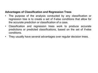
SlideShare a Scribd company logo
CSA 3702 – MACHINE LEARNING
PREPARED BY,
NANDHINI S (SRMIST, RAMAPURAM CAMPUS),
BHARATHI RAJA N, MENNAKSHI COLLEGE OF ENGINEERING.
MODULE - II
Classification Algorithms
Decision Trees
Why decision tree?
• Decision trees are powerful and popular tools for classification and
prediction.
• Decision trees represent rules, which can be understood by humans
and used in knowledge system such as database.
Key requirements
• Attribute-value description: object or case must be expressible in
terms of a fixed collection of properties or attributes (e.g., hot, mild,
cold).
• Predefined classes (target values): the target function has
discrete output values (boolean or multiclass)
• Sufficient data: enough training cases should be provided to learn
the model.
Definition
• Decision tree is a classifier in the form of a tree structure
– Decision node: specifies a test on a single attribute
– Leaf node: indicates the value of the target attribute
– Arc/edge: split of one attribute
– Path: a disjunction of test to make the final decision
• Decision trees classify instances or examples by starting
at the root of the tree and moving through it until a leaf
node.
Decision Tree
• A tree has many analogies in real life, and turns out that it has
influenced a wide area of machine learning, covering
both classification and regression.
• In decision analysis, a decision tree can be used to visually and
explicitly represent decisions and decision making.
• Decision Trees are a type of Supervised Machine Learning (that is
you explain what the input is and what the corresponding output is in
the training data) where the data is continuously split according to a
certain parameter.
• The tree can be explained by two entities, namely decision nodes
and leaves. The leaves are the decisions or the final outcomes. And
the decision nodes are where the data is split.
• An example of a decision tree can be explained using above
binary tree. Let’s say you want to predict whether a person is fit
given their information like age, eating habit, and physical activity,
etc.
• The decision nodes here are questions like ‘What’s the age?’,
‘Does he exercise?’, ‘Does he eat a lot of pizzas’? And the
leaves, which are outcomes like either ‘fit’, or ‘unfit’. In this case
this is a binary classification problem (a yes no type problem).
• There are two main types of Decision Trees:
1.Classification trees (Yes/No types)
– What we’ve seen above is an example of classification tree, where the outcome
is a variable like ‘fit’ or ‘unfit’. Here the decision variable is Categorical.
2. Regression trees (Continuous data types)
– Here the decision or the outcome variable is Continuous, e.g. a number like
123.
• Decision Trees are a non-parametric supervised learning
method used for both classification and regression tasks.
• The goal is to create a model that predicts the value of a target
variable by learning simple decision rules inferred from the data
features.
• A decision tree is a tree-like graph with nodes representing the
place where we pick an attribute and ask a question; edges
represent the answers the to the question; and the leaves
represent the actual output or class label.
• They are used in non-linear decision making with simple linear
decision surface.
A simple example
• You want to guess the outcome of next week's game between the
MallRats and the Chinooks.
• Available knowledge / Attribute
– was the game at Home or Away
– was the starting time 5pm, 7pm or 9pm.
– Did Joe play center, or forward.
– whether that opponent's center was tall or not.
– …..
Basket ball data
What we know
• The game will be away, at 9pm, and that Joe will play
center on offense…
• A classification problem
• Generalizing the learned rule to new examples
• Illustration
(2) Which node to proceed?
(3) When to stop/ come to conclusion?
(1) Which to start? (root)
Random split
• The tree can grow huge.
• These trees are hard to understand.
• Larger trees are typically less accurate than smaller trees.
Principled Criterion
• Selection of an attribute to test at each node - choosing the most
useful attribute for classifying examples.
• information gain
– measures how well a given attribute separates the training
examples according to their target classification
– This measure is used to select among the candidate attributes at
each step while growing the tree
Entropy
• A measure of homogeneity of the set of examples.
• Given a set S of positive and negative examples of some target
concept (a 2-class problem), the entropy of set S relative to this
binary classification is
E(S) = - p(P)log2 p(P) – p(N)log2 p(N)
• Suppose S has 25 examples, 15 positive and 10 negatives
[15+, 10-]. Then the entropy of S relative to this classification is
E(S)=-(15/25) log2(15/25) - (10/25) log2 (10/25)
• The entropy is 0 if the outcome is ``certain’’.
• The entropy is maximum if we have no knowledge of the system (or
any outcome is equally possible).
Entropy of a 2-class problem
with regard to the portion of
one of the two groups
Information Gain
• Information gain measures the expected reduction in entropy, or
uncertainty.
– Values(A) is the set of all possible values for attribute A, and Sv
the subset of S for which attribute A has value v Sv = {s in S |
A(s) = v}.
– the first term in the equation for Gain is just the entropy of the
original collection S
– the second term is the expected value of the entropy after S is
partitioned using attribute A
• It is simply the expected reduction in entropy caused by partitioning
the examples according to this attribute.
• It is the number of bits saved when encoding the target value of an
arbitrary member of S, by knowing the value of attribute A.
( )
( , ) ( ) ( )v
v
v Values A
S
Gain S A Entropy S Entropy S
S
= − 
Examples
• Before partitioning, the entropy is
H(10/20, 10/20) = - 10/20 log(10/20) - 10/20 log(10/20) = 1
• Using the ``where’’ attribute, divide into 2 subsets
Entropy of the first set H(home) = - 6/12 log(6/12) - 6/12 log(6/12) = 1
Entropy of the second set H(away) = - 4/8 log(6/8) - 4/8 log(4/8) = 1
• Expected entropy after partitioning
12/20 * H(home) + 8/20 * H(away) = 1
• Using the ``when’’ attribute, divide into 3 subsets
Entropy of the first set H(5pm) = - 1/4 log(1/4) - 3/4 log(3/4);
Entropy of the second set H(7pm) = - 9/12 log(9/12) - 3/12 log(3/12);
Entropy of the second set H(9pm) = - 0/4 log(0/4) - 4/4 log(4/4) = 0
• Expected entropy after partitioning
4/20 * H(1/4, 3/4) + 12/20 * H(9/12, 3/12) + 4/20 * H(0/4, 4/4) = 0.65
• Information gain 1-0.65 = 0.35
Decision
• Knowing the ``when’’ attribute values provides larger information
gain than ``where’’.
• Therefore the ``when’’ attribute should be chosen for testing
prior to the ``where’’ attribute.
• Similarly, we can compute the information gain for other
attributes.
• At each node, choose the attribute with the largest information
Stopping rule
– Every attribute has already been included along this path
through the tree, or
– The training examples associated with this leaf node all have the
same target attribute value (i.e., their entropy is zero).
Continuous Attribute..?
• Each non-leaf node is a test, its edge partitioning the attribute into
subsets (easy for discrete attribute).
• For continuous attribute
– Partition the continuous value of attribute A into a discrete set of
intervals
– Create a new boolean attribute Ac , looking for a threshold c,
if
otherwise
c
c
true A c
A
false

= 

Evaluation
• Training accuracy
– How many training instances can be correctly classify based on
the available data?
– Is high when the tree is deep/large, or when there is less
confliction in the training instances.
– however, higher training accuracy does not mean good
generalization
• Testing accuracy
– Given a number of new instances, how many of them can we
correctly classify?
– Cross validation
Issues in decision trees learning
• Overfitting
• Reduced error pruning
• Rule post-pruning
• Extensions
• Continuous valued attributes
• Alternative measures for selecting attributes
• Handling training examples with missing attribute values
• Handling attributes with different costs
• Improving computational efficiency
Overfitting: definition
• Building trees that “adapt too much” to the training examples may
lead to “overfitting”.
• Consider error of hypothesis h over
– training data: errorD(h) empirical error
– entire distribution X of data: errorX(h) expected error
• Hypothesis h overfits training data if there is an alternative
hypothesis h'  H such that
errorD(h) < errorD(h’) and
errorX(h’) < errorX(h)
-i.e. h’ behaves better over unseen data
Avoid overfitting in Decision Trees
• Two strategies:
1. Stop growing the tree earlier, before perfect classification
2. Allow the tree to overfit the data, and then post-prune the tree
• Training and validation set
• split the training in two parts (training and validation) and use
validation to assess the utility of post-pruning
1. Reduced error pruning
2. Rule pruning
• Other approaches
• Use a statistical test to estimate effect of expanding or pruning
• Minimum description length principle: uses a measure of
complexity of encoding the DT and the examples, and halt
growing the tree when this encoding size is minimal
Strengths
• can generate understandable rules
• perform classification without much computation
• can handle continuous and categorical variables
• provide a clear indication of which fields are most important for
prediction or classification
• Inexpensive to construct
• Extremely fast at classifying unknown records
• Easy to interpret for small-sized trees
• Okay for noisy data
• Can handle both continuous and symbolic attributes
• Accuracy is comparable to other classification techniques for many
simple data sets
• Decent average performance over many datasets
Weakness
• Not suitable for prediction of continuous attribute.
• Perform poorly with many class and small data.
• Computationally expensive to train.
– At each node, each candidate splitting field must be sorted
before its best split can be found.
– In some algorithms, combinations of fields are used and a
search must be made for optimal combining weights.
– Pruning algorithms can also be expensive since many candidate
sub-trees must be formed and compared.
• Do not treat well non-rectangular regions.
• Relies on rectangular approximation that might not be good for
some dataset
• Selecting good learning algorihtm parameters (e.g. degree of
pruning) is non-trivial
Classification and Regression
Trees
• The CART or Classification & Regression Trees methodology refers
to these two types of decision trees.
(i) Classification Trees
• A classification tree is an algorithm where the target variable is fixed
or categorical. The algorithm is then used to identify the “class”
within which a target variable would most likely fall.
• An example of a classification-type problem would be determining
who will or will not subscribe to a digital platform; or who will or will
not graduate from high school.
• These are examples of simple binary classifications where the
categorical dependent variable can assume only one of two,
mutually exclusive values.
• In other cases, you might have to predict among a number of
different variables. For instance, you may have to predict which type
of smartphone a consumer may decide to purchase.
• In such cases, there are multiple values for the categorical
dependent variable.
Fig. Classification Trees
(ii) Regression Trees
• A regression tree refers to an algorithm where the target variable is
and the algorithm is used to predict it’s value.
• As an example of a regression type problem, you may want to
predict the selling prices of a residential house, which is a
continuous dependent variable.
• This will depend on both continuous factors like square footage as
well as categorical factors like the style of home, area in which the
property is located and so on.
When to use Classification and Regression Trees
• Classification trees are used when the dataset needs to be split into
classes which belong to the response variable. In many cases, the
classes Yes or No.
• In other words, they are just two and mutually exclusive. In some
cases, there may be more than two classes in which case a variant
of the classification tree algorithm is used.
• Regression trees, on the other hand, are used when the response
variable is continuous.
• For instance, if the response variable is something like the price of a
property or the temperature of the day, a regression tree is used.
• In other words, regression trees are used for prediction-type
problems while classification trees are used for classification-type
problems.
How Classification and Regression Trees
• A classification tree splits the dataset based on the homogeneity of
data.
• for instance, there are two variables; income and age; which
determine whether or not a consumer will buy a particular kind of
phone.
• If the training data shows that 95% of people who are older than 30
bought the phone, the data gets split there and age becomes a top
node in the tree.
• This split makes the data “95% pure”. Measures of impurity like
entropy or Gini index are used to quantify the homogeneity of the
data when it comes to classification trees.
• In a regression tree, a regression model is fit to the target variable
using each of the independent variables. After this, the data is split
at several points for each independent variable.
• At each such point, the error between the predicted values and
actual values is squared to get “A Sum of Squared Errors”(SSE).
• The SSE is compared across the variables and the variable or point
which has the lowest SSE is chosen as the split point. This process
is continued recursively.
Figure : CART working
Advantages of Classification and Regression Trees
• The purpose of the analysis conducted by any classification or
regression tree is to create a set of if-else conditions that allow for
the accurate prediction or classification of a case.
• Classification and regression trees work to produce accurate
predictions or predicted classifications, based on the set of if-else
conditions.
• They usually have several advantages over regular decision trees.
(i) The Results are Simplistic
• The interpretation of results summarized in classification or
regression trees is usually fairly simple.
- The simplicity of results helps in the following ways.
• It allows for the rapid classification of new observations. That’s
because it is much simpler to evaluate just one or two logical
conditions than to compute scores using complex nonlinear
equations for each group.
• It can often result in a simpler model which explains why the
observations are either classified or predicted in a certain way. For
instance, business problems are much easier to explain with if-then
statements than with complex nonlinear equations.
(ii) Classification and Regression Trees are Nonparametric &
Nonlinear
• The results from classification and regression trees can be
summarized in simplistic if-then conditions. This negates the need
for the following implicit assumptions.
• The predictor variables and the dependent variable are linear.
• The predictor variables and the dependent variable follow some
specific nonlinear link function.
• The predictor variables and the dependent variable are monotonic.
• Since there is no need for such implicit assumptions, classification
and regression tree methods are well suited to data mining. This is
because there is very little knowledge or assumptions that can be
made beforehand about how the different variables are related.
(iii) Classification and Regression Trees Implicitly Perform Feature
Selection
• Feature selection or variable screening is an important part of
analytics.
• When we use decision trees, the top few nodes on which the tree is
split are the most important variables within the set.
• As a result, feature selection gets performed automatically and we
don’t need to do it again.
Limitations of Classification and Regression Trees
• There are many classification and regression trees examples where
the use of a decision tree has not led to the optimal result.
• Here are some of the limitations of classification and regression
trees.
1. Over fitting
2. High invariance
3. Low bias
(i) Overfitting
• Overfitting occurs when the tree takes into account a lot of noise that
exists in the data and comes up with an inaccurate result.
(ii) High variance
• In this case, a small variance in the data can lead to a very high
variance in the prediction, thereby affecting the stability of the
outcome.
(iii) Low bias
• A decision tree that is very complex usually has a low bias. This
makes it very difficult for the model to incorporate any new data.
What is a CART in Machine Learning..?
• A Classification and Regression Tree(CART) is a predictive
algorithm used in machine learning.
• It explains how a target variable’s values can be predicted based on
other values.
• It is a decision tree where each fork is a split in a predictor variable
and each node at the end has a prediction for the target variable.
• The CART algorithm is an important decision tree algorithm that lies
at the foundation of machine learning.
• It is also the basis for other powerful machine learning algorithms
like bagged decision trees, random forest and boosted decision
trees.
Probability and Learning
Reasons to Learn Probability
1. Class Membership Requires Predicting a Probability
- Classification predictive modeling problems are those where an
example is assigned a given label.
• An example : The Iris flowers dataset (Refer Google-
https://archive.ics.uci.edu/ml/datasets/iris) where we have four
measurements of a flower and the goal is to assign one of three
different known species of iris flower to the observation.
• We can model the problem as directly assigning a class label to
each observation.
– Input: Measurements of a flower.
– Output: One iris species.
• A more common approach is to frame the problem as a probabilistic
class membership, where the probability of an observation
belonging to each known class is predicted.
– Input: Measurements of a flower.
– Output: Probability of membership to each iris species.
• Framing the problem as a prediction of class membership simplifies
the modeling problem and makes it easier for a model to learn.
• It allows the model to capture ambiguity in the data, which allows a
process downstream, such as the user to interpret the probabilities
in the context of the domain.
• The probabilities can be transformed into a crisp class label by
choosing the class with the largest probability.
• The probabilities can also be scaled or transformed using
a probability calibration process.
• This choice of a class membership framing of the problem
interpretation of the predictions made by the model requires a basic
understanding of probability.
2. Models Are Designed Using Probability
• There are algorithms that are specifically designed to harness the
tools and methods from probability.
• These range from individual algorithms, like Naive Bayes algorithm,
which is constructed using Bayes Theorem with some simplifying
assumptions.
- Naive Bayes
• The linear regression algorithm can be seen as a probabilistic model
that minimizes the mean squared error of predictions, and the
logistic regression algorithm can be seen as a probabilistic model
that minimizes the negative log likelihood of predicting the positive
class label.
- Linear Regression
-Logistic Regression
• It also extends to whole fields of study, such as probabilistic
graphical models,.
• A notable graphical model is Bayesian Belief Networks or Bayes
Nets, which are capable of capturing the conditional dependencies
between variables.
3. Models Are Trained With Probabilistic Frameworks
• Many machine learning models are trained using an iterative
algorithm designed under a probabilistic framework.
• Some examples of general probabilistic modeling frameworks are:
• Maximum Likelihood Estimation (Frequentist).
• Maximum a Posteriori Estimation (Bayesian).
• Perhaps the most common is the framework of maximum likelihood
estimation, sometimes shorted as MLE. This is a framework for
estimating model parameters (e.g. weights) given observed data.
• This is the framework that underlies the ordinary least squares
estimate of a linear regression model and the log loss estimate for
logistic regression.
• The expectation-maximization algorithm is an approach for
maximum likelihood estimation often used for unsupervised data
clustering, e.g. estimating k means for k clusters, also known as
the k-Means clustering algorithm.
4. Models Are Tuned With a Probabilistic Framework
• It is common to tune the hyperparameters of a machine learning
model, such as k for kNN or the learning rate in a neural network.
• Typical approaches include grid searching ranges of
hyperparameters or randomly sampling hyperparameter
combinations.
• Bayesian optimization is a more efficient to hyperparameter
optimization that involves a directed search of the space of possible
configurations based on those configurations that are most likely to
result in better performance.
• As its name suggests, the approach was devised from and
harnesses Bayes Theorem when sampling the space of possible
configurations.
5. Models Are Evaluated With Probabilistic Measures
• For those algorithms where a prediction of probabilities is made,
evaluation measures are required to summarize the performance of
the model.
• There are many measures used to summarize the performance of a
model based on predicted probabilities. Common examples include:
– Log Loss (also called cross-entropy).
– Brier Score, and the Brier Skill Score
• For binary classification tasks where a single probability score is
predicted, Receiver Operating Characteristic, or ROC, curves can
be constructed to explore different cut-offs that can be used when
interpreting the prediction that, in turn, result in different trade-offs.
• The area under the ROC curve, or ROC AUC, can also be
calculated as an aggregate measure.
– ROC Curve and ROC AUC
– Precision-Recall Curve and AUC
Some basic Statistics
Statistics
• Statistics is a field of mathematics that is universally agreed to be a
prerequisite for a deeper understanding of machine learning.
Why do we need Statistics?
• Statistics is a collection of tools that you can use to get answers to
important questions about data.
• We can use descriptive statistical methods to transform raw
observations into information that you can understand and share.
• We can can use inferential statistical methods to reason from small
samples of data to whole domains.
where statistical methods are used in an applied machine
learning…
• Problem Framing: Requires the use of exploratory data analysis
and data mining.
• Data Understanding: Requires the use of summary statistics and
data visualization.
• Data Cleaning. Requires the use of outlier detection, imputation and
more.
• Data Selection. Requires the use of data sampling and feature
selection methods.
• Data Preparation. Requires the use of data transforms, scaling,
encoding and much more.
• Model Evaluation. Requires experimental design and resampling
methods.
• Model Configuration. Requires the use of statistical hypothesis
tests and estimation statistics.
• Model Selection. Requires the use of statistical hypothesis tests
and estimation statistics.
• Model Presentation. Requires the use of estimation statistics such
as confidence intervals.
• Model Predictions. Requires the use of estimation statistics such
as prediction intervals.
Statistics and Machine Learning
1. Statistics in Data Preparation
• Statistical methods are required in the preparation of train and test
data for your machine learning model.
– This includes techniques for:
– Outlier detection.
– Missing value imputation.
– Data sampling.
– Data scaling.
– Variable encoding.
2. Statistics in Model Evaluation
• Statistical methods are required when evaluating the skill of a
machine learning model on data not seen during training.
– This includes techniques for:
– Data sampling.
– Data resampling.
– Experimental design.
3. Statistics in Model Selection
• Statistical methods are required when selecting a final model or
model configuration to use for a predictive modeling problem.
– These include techniques for:
– Checking for a significant difference between results.
– Quantifying the size of the difference between results.
4. Statistics in Model Presentation
• Statistical methods are required when presenting the skill of a final
model to stakeholders.
– This includes techniques for:
– Summarizing the expected skill of the model on average.
– Quantifying the expected variability of the skill of the model in practice.
5. Statistics in Prediction
• Statistical methods are required when making a prediction with a
finalized model on new data.
– This includes techniques for:
– Quantifying the expected variability for the prediction.
Gaussian Distribution and Descriptive Stats
• Variables in a dataset may be related for lots of reasons.
• It can be useful in data analysis and modeling to better understand
the relationships between variables. The statistical relationship
between two variables is referred to as their correlation.
• A correlation could be positive, meaning both variables move in the
same direction, or negative, meaning that when one variable’s value
increases, the other variables’ values decrease.
• Positive Correlation: Both variables change in the same direction.
• Neutral Correlation: No relationship in the change of the variables.
• Negative Correlation: Variables change in opposite directions.
Statistical Hypothesis Tests
• Data must be interpreted in order to add meaning. We can interpret
data by assuming a specific structure our outcome and use
statistical methods to confirm or reject the assumption.
• The assumption is called a hypothesis and the statistical tests used
for this purpose are called statistical hypothesis tests.
• The assumption of a statistical test is called the null hypothesis, or
hypothesis zero (H0 for short).
• It is often called the default assumption, or the assumption that
nothing has changed. A violation of the test’s assumption is often
called the first hypothesis, hypothesis one, or H1 for short.
– Hypothesis 0 (H0): Assumption of the test holds and is failed to be rejected.
– Hypothesis 1 (H1): Assumption of the test does not hold and is rejected at some
level of significance.
Bayesian procedures
• Bayesian classification procedures provide a natural way of taking
into account any available information about the relative sizes of the
different groups within the overall population.
• Bayesian procedures tend to be computationally expensive and, in
the days before Markov chain Monte Carlo computations were
developed, approximations for Bayesian clustering rules were
devised.
Binary and multiclass classification
• In binary classification, only two classes are involved, whereas
multiclass classification involves assigning an object to one of
several classes.
• Since many classification methods have been developed specifically
for binary classification, multiclass classification often requires the
combined use of multiple binary classifiers.
Feature vectors
• Most algorithms describe an individual instance whose category is
to be predicted using a feature vector of individual, measurable
properties of the instance.
• Each property is termed a feature, also known in statistics as
an explanatory variable .
• If the instance is an image, the feature values might correspond to
the pixels of an image; if the instance is a piece of text, the feature
values might be occurrence frequencies of different words.
Linear classifiers
• A large number of algorithms for classification can be phrased in
terms of a linear function that assigns a score to each possible
category k by combining the feature vector of an instance with a
vector of weights, using a dot product.
• The predicted category is the one with the highest score. This type
of score function is known as a linear predictor function.
Estimation Statistics
• Statistical hypothesis tests can be used to indicate whether the
difference between two samples is due to random chance, but
cannot comment on the size of the difference.
• Estimation statistics is a term to describe three main classes of
methods.
• The three main classes of methods include:
– Effect Size. Methods for quantifying the size of an effect given a treatment or
intervention.
– Interval Estimation. Methods for quantifying the amount of uncertainty in a
value.
– Meta-Analysis. Methods for quantifying the findings across multiple similar
studies.
Nonparametric Statistics
• Data in which the distribution is unknown or cannot be easily
identified is called nonparametric.
• In the case where you are working with nonparametric data,
specialized nonparametric statistical methods can be used that
discard all information about the distribution. As such, these
methods are often referred to as distribution-free methods.
• Before a nonparametric statistical method can be applied, the data
must be converted into a rank format. As such, statistical methods
that expect data in rank format are sometimes called rank statistics,
such as rank correlation and rank statistical hypothesis tests.
Ranking data is exactly as its name suggests.
• The procedure is as follows:
– Sort all data in the sample in ascending order.
– Assign an integer rank from 1 to N for each unique value in the data sample.
Gaussian Mixture Model
• A Gaussian Mixture Model (GMM) is a parametric representation
of a probability density function, based on a weighted sum of multi-
variate Gaussian distributions.
• GMMs are commonly used as a parametric model of the probability
distribution of continuous measurements or features in a biometric
system.
• GMM parameters are estimated from training data using the iterative
Expectation-Maximization (EM) algorithm or Maximum A Posteriori
(MAP) estimation from a well-trained prior model.
• GMM is computationally inexpensive, does not require phonetically
labeled training speech, and is well suited for text-independent
tasks, where there is no strong prior knowledge of the spoken text.
• GMM is used in Signal Processing , Speaker Recognition,
Language Identification, Classification etc..
• Big phoneme or vocabulary database no needed.
• Text independent verification.
• Gaussian Mixture Models (GMMs) assume that there are a certain
number of Gaussian distributions, and each of these distributions
represent a cluster.
• Hence, a Gaussian Mixture Model tends to group the data points
belonging to a single distribution together.
• Gaussian Mixture Models are probabilistic models and use the soft
clustering approach for distributing the points in different clusters.
• It has a bell-shaped curve, with the data points symmetrically
distributed around the mean value.
• In a one dimensional space, the probability density function of a
Gaussian distribution is given by:
- where μ is the mean and σ2 is the variance.
• The below image has a few Gaussian distributions with a difference
in mean (μ) and variance (σ2). Remember that the higher the σ
value more would be the spread:
• In the case of two variables, instead of a 2D bell-shaped curve, we
will have a 3D bell curve as shown below:
• The probability density function would be given by:
- where x is the input vector, μ is the 2D mean vector, and Σ is the 2×2
covariance matrix.
• Thus, this multivariate Gaussian model would have x and μ as
vectors of length d, and Σ would be a d x d covariance matrix.
• Hence, for a dataset with d features, we would have a mixture
of k Gaussian distributions (where k is equivalent to the number of
clusters), each having a certain mean vector and variance matrix.
– how is the mean and variance value for each Gaussian assigned?
• These values are determined using a technique called Expectation-
Maximization (EM).
• Expectation-Maximization (EM) is a statistical algorithm for finding
the right model parameters. We typically use EM when the data has
missing values (called latent variables), or in other words, when the
data is incomplete.
• An Expectation–Maximization (EM) algorithm is an iterative method
for finding Maximum Likelihood or Maximum A Posteriori(MAP)
estimates of parameters in statistical models, where the model
depends on unobserved latent variables
EM Algorithm consists of two major steps:
1 st --E (Expectation) step
2 nd--M (Maximization) step
• E (Expectation) step: In the E-step, the expected value of the log-
likelihood function is calculated given the observed data and current
estimate of the model parameters.
• M (Maximization) step: The M-step computes the parameters
which maximize the expected log-likelihood found on the E-step.
These parameters are then used to determine the distribution of the
latent variables in the next E-step until the algorithm has converged.
Expectation-Maximization in Gaussian Mixture
Models
E-step
• For each point xi, calculate the probability that it belongs to
cluster/distribution c1, c2, … ck. This is done using the below formula:
- This value will be high when the point is assigned to the right
cluster and lower otherwise.
M-step:
• Post the E-step, we go back and update the Π, μ and Σ values.
These are updated in the following manner:
• The new density is defined by the ratio of the number of points in the
cluster and the total number of points:
• The mean and the covariance matrix are updated based on the
values assigned to the distribution, in proportion with the probability
values for the data point.
• Hence, a data point that has a higher probability of being a part of
that distribution will contribute a larger portion:
Maximum Posteriori Probability
• A maximum a posteriori probability (MAP) estimate is a mode of
the posterior distribution
• The MAP estimation is a two step estimation process:
1 st-- Estimates of the sufficient statistics of the training data
are computed for each mixture in the prior model.
2 nd-- For adaptation these ‘new’ sufficient statistic estimates
are then combined with the ‘old’ sufficient statistics from the prior
mixture parameters using a data-dependent mixing coefficient.
Maximum Likelihood
• In statistics, maximum-likelihood estimation (MLE) is a method of
estimating the parameters of a statistical model. When applied to a
data set and given a statistical model, maximum-likelihood
estimation provides estimates for the model's parameters.
Nearest Neighbour Method
K-Nearest Neighbours
• K-Nearest Neighbors is one of the most basic yet essential
classification algorithms in Machine Learning.
• It belongs to the supervised learning domain and finds intense
application in pattern recognition, data mining and intrusion
detection.
• The KNN algorithm assumes that similar things exist in close
proximity. In other words, similar things are near to each other.
Image showing how similar data points typically exist close to each other
• From the mentioned figure- most of the time, similar data points are
close to each other.
• The KNN algorithm hinges on this assumption being true enough for
the algorithm to be useful.
• KNN captures the idea of similarity (sometimes called distance,
proximity, or closeness) with some mathematics.
The KNN Algorithm
1. Load the data
2. Initialize K to your chosen number of neighbors
3. For each example in the data
• 3.1 Calculate the distance between the query example and the
current example from the data.
• 3.2 Add the distance and the index of the example to an ordered
collection
4. Sort the ordered collection of distances and indices from smallest to
largest (in ascending order) by the distances
5. Pick the first K entries from the sorted collection
6. Get the labels of the selected K entries
7. If regression, return the mean of the K labels
8. If classification, return the mode of the K labels
Choosing the right value for K
• To select the K that’s right for your data, we run the KNN algorithm
several times with different values of K and choose the K that
reduces the number of errors we encounter while maintaining the
algorithm’s ability to accurately make predictions when it’s given
data it hasn’t seen before.
– As we decrease the value of K to 1, our predictions become less stable. Just
think for a minute, imagine K=1 and we have a query point surrounded by
several reds and one green (I’m thinking about the top left corner of the colored
plot above), but the green is the single nearest neighbor. Reasonably, we would
think the query point is most likely red, but because K=1, KNN incorrectly
predicts that the query point is green.
– Inversely, as we increase the value of K, our predictions become more stable
due to majority voting / averaging, and thus, more likely to make more accurate
predictions (up to a certain point). Eventually, we begin to witness an increasing
number of errors. It is at this point we know we have pushed the value of K too
far.
– In cases where we are taking a majority vote (e.g. picking the mode in a
classification problem) among labels, we usually make K an odd number to have
a tiebreaker.
Advantages
• The algorithm is simple and easy to implement.
• There’s no need to build a model, tune several parameters, or make
additional assumptions.
• The algorithm is versatile. It can be used for classification,
regression, and search (as we will see in the next section).
Disadvantages
• The algorithm gets significantly slower as the number of examples
and/or predictors/independent variables increase.

More Related Content

PDF
CSA 3702 machine learning module 1
PPTX
Distributed DBMS - Unit 1 - Introduction
PPTX
Ant colony optimization
PDF
Machine Learning Course | Edureka
PPTX
Fuzzy Genetic Algorithm
PDF
deep learning
PPTX
Database , 8 Query Optimization
CSA 3702 machine learning module 1
Distributed DBMS - Unit 1 - Introduction
Ant colony optimization
Machine Learning Course | Edureka
Fuzzy Genetic Algorithm
deep learning
Database , 8 Query Optimization

What's hot (20)

PDF
CSA 3702 machine learning module 4
PPTX
05 Clustering in Data Mining
PDF
Unsupervised learning: Clustering
PPT
CONFUSION MATRIX.ppt
PDF
CSA 3702 machine learning module 3
PPTX
Hierarchical clustering
PPTX
Ensemble Learning and Random Forests
PPTX
Machine learning algorithms
PPT
Ann
PPTX
K-Means Clustering Algorithm.pptx
PPT
Cluster analysis
PDF
Run time storage
PPTX
Machine learning clustering
PPTX
Decision trees
PPTX
PDF
Hill Climbing Algorithm in Artificial Intelligence
PPTX
Handling Missing Values for Machine Learning.pptx
PDF
Decision Tree in Machine Learning
PPTX
Classification Algorithm.
PDF
Intro to AI STRIPS Planning & Applications in Video-games Lecture6-Part1
CSA 3702 machine learning module 4
05 Clustering in Data Mining
Unsupervised learning: Clustering
CONFUSION MATRIX.ppt
CSA 3702 machine learning module 3
Hierarchical clustering
Ensemble Learning and Random Forests
Machine learning algorithms
Ann
K-Means Clustering Algorithm.pptx
Cluster analysis
Run time storage
Machine learning clustering
Decision trees
Hill Climbing Algorithm in Artificial Intelligence
Handling Missing Values for Machine Learning.pptx
Decision Tree in Machine Learning
Classification Algorithm.
Intro to AI STRIPS Planning & Applications in Video-games Lecture6-Part1
Ad

Similar to CSA 3702 machine learning module 2 (20)

PPTX
MACHINE LEARNING - ENTROPY & INFORMATION GAINpptx
PPTX
Lect9 Decision tree
PPTX
DECISION TREE AND PROBABILISTIC MODELS.pptx
PDF
Decision Tree-ID3,C4.5,CART,Regression Tree
PDF
From decision trees to random forests
PPT
Using Tree algorithms on machine learning
PPTX
Unit 4 Classification of data and more info on it
PPT
Decision tree
PPT
Decision tree
PPTX
DecisionTree.pptx for btech cse student
PPT
Decision_Tree in machine learning with examples.ppt
PPTX
Machine Learning with Python unit-2.pptx
PPTX
Decision Trees
PDF
7 decision tree
PPTX
Machine Learning
PDF
Machine Learning Unit-5 Decesion Trees & Random Forest.pdf
PDF
lec8_annotated.pdf ml csci 567 vatsal sharan
PPTX
Decision tree induction
PDF
Chapter 4.pdf
PPTX
Decision Tree Learning
MACHINE LEARNING - ENTROPY & INFORMATION GAINpptx
Lect9 Decision tree
DECISION TREE AND PROBABILISTIC MODELS.pptx
Decision Tree-ID3,C4.5,CART,Regression Tree
From decision trees to random forests
Using Tree algorithms on machine learning
Unit 4 Classification of data and more info on it
Decision tree
Decision tree
DecisionTree.pptx for btech cse student
Decision_Tree in machine learning with examples.ppt
Machine Learning with Python unit-2.pptx
Decision Trees
7 decision tree
Machine Learning
Machine Learning Unit-5 Decesion Trees & Random Forest.pdf
lec8_annotated.pdf ml csci 567 vatsal sharan
Decision tree induction
Chapter 4.pdf
Decision Tree Learning
Ad

Recently uploaded (20)

PDF
Structs to JSON How Go Powers REST APIs.pdf
PPTX
MET 305 2019 SCHEME MODULE 2 COMPLETE.pptx
PPTX
UNIT 4 Total Quality Management .pptx
PPTX
CH1 Production IntroductoryConcepts.pptx
PPTX
Foundation to blockchain - A guide to Blockchain Tech
PPTX
Lesson 3_Tessellation.pptx finite Mathematics
PPT
Mechanical Engineering MATERIALS Selection
PPTX
Engineering Ethics, Safety and Environment [Autosaved] (1).pptx
PPTX
IOT PPTs Week 10 Lecture Material.pptx of NPTEL Smart Cities contd
PDF
Mitigating Risks through Effective Management for Enhancing Organizational Pe...
PDF
Digital Logic Computer Design lecture notes
PDF
Well-logging-methods_new................
PPTX
web development for engineering and engineering
PPTX
UNIT-1 - COAL BASED THERMAL POWER PLANTS
PPTX
CARTOGRAPHY AND GEOINFORMATION VISUALIZATION chapter1 NPTE (2).pptx
PPTX
Lecture Notes Electrical Wiring System Components
DOCX
573137875-Attendance-Management-System-original
PPT
Project quality management in manufacturing
PPTX
FINAL REVIEW FOR COPD DIANOSIS FOR PULMONARY DISEASE.pptx
PPTX
additive manufacturing of ss316l using mig welding
Structs to JSON How Go Powers REST APIs.pdf
MET 305 2019 SCHEME MODULE 2 COMPLETE.pptx
UNIT 4 Total Quality Management .pptx
CH1 Production IntroductoryConcepts.pptx
Foundation to blockchain - A guide to Blockchain Tech
Lesson 3_Tessellation.pptx finite Mathematics
Mechanical Engineering MATERIALS Selection
Engineering Ethics, Safety and Environment [Autosaved] (1).pptx
IOT PPTs Week 10 Lecture Material.pptx of NPTEL Smart Cities contd
Mitigating Risks through Effective Management for Enhancing Organizational Pe...
Digital Logic Computer Design lecture notes
Well-logging-methods_new................
web development for engineering and engineering
UNIT-1 - COAL BASED THERMAL POWER PLANTS
CARTOGRAPHY AND GEOINFORMATION VISUALIZATION chapter1 NPTE (2).pptx
Lecture Notes Electrical Wiring System Components
573137875-Attendance-Management-System-original
Project quality management in manufacturing
FINAL REVIEW FOR COPD DIANOSIS FOR PULMONARY DISEASE.pptx
additive manufacturing of ss316l using mig welding

CSA 3702 machine learning module 2

  • 1. CSA 3702 – MACHINE LEARNING PREPARED BY, NANDHINI S (SRMIST, RAMAPURAM CAMPUS), BHARATHI RAJA N, MENNAKSHI COLLEGE OF ENGINEERING.
  • 4. Why decision tree? • Decision trees are powerful and popular tools for classification and prediction. • Decision trees represent rules, which can be understood by humans and used in knowledge system such as database. Key requirements • Attribute-value description: object or case must be expressible in terms of a fixed collection of properties or attributes (e.g., hot, mild, cold). • Predefined classes (target values): the target function has discrete output values (boolean or multiclass) • Sufficient data: enough training cases should be provided to learn the model.
  • 5. Definition • Decision tree is a classifier in the form of a tree structure – Decision node: specifies a test on a single attribute – Leaf node: indicates the value of the target attribute – Arc/edge: split of one attribute – Path: a disjunction of test to make the final decision • Decision trees classify instances or examples by starting at the root of the tree and moving through it until a leaf node.
  • 6. Decision Tree • A tree has many analogies in real life, and turns out that it has influenced a wide area of machine learning, covering both classification and regression. • In decision analysis, a decision tree can be used to visually and explicitly represent decisions and decision making. • Decision Trees are a type of Supervised Machine Learning (that is you explain what the input is and what the corresponding output is in the training data) where the data is continuously split according to a certain parameter. • The tree can be explained by two entities, namely decision nodes and leaves. The leaves are the decisions or the final outcomes. And the decision nodes are where the data is split.
  • 7. • An example of a decision tree can be explained using above binary tree. Let’s say you want to predict whether a person is fit given their information like age, eating habit, and physical activity, etc. • The decision nodes here are questions like ‘What’s the age?’, ‘Does he exercise?’, ‘Does he eat a lot of pizzas’? And the leaves, which are outcomes like either ‘fit’, or ‘unfit’. In this case this is a binary classification problem (a yes no type problem).
  • 8. • There are two main types of Decision Trees: 1.Classification trees (Yes/No types) – What we’ve seen above is an example of classification tree, where the outcome is a variable like ‘fit’ or ‘unfit’. Here the decision variable is Categorical. 2. Regression trees (Continuous data types) – Here the decision or the outcome variable is Continuous, e.g. a number like 123. • Decision Trees are a non-parametric supervised learning method used for both classification and regression tasks. • The goal is to create a model that predicts the value of a target variable by learning simple decision rules inferred from the data features. • A decision tree is a tree-like graph with nodes representing the place where we pick an attribute and ask a question; edges represent the answers the to the question; and the leaves represent the actual output or class label. • They are used in non-linear decision making with simple linear decision surface.
  • 9. A simple example • You want to guess the outcome of next week's game between the MallRats and the Chinooks. • Available knowledge / Attribute – was the game at Home or Away – was the starting time 5pm, 7pm or 9pm. – Did Joe play center, or forward. – whether that opponent's center was tall or not. – …..
  • 11. What we know • The game will be away, at 9pm, and that Joe will play center on offense… • A classification problem • Generalizing the learned rule to new examples
  • 12. • Illustration (2) Which node to proceed? (3) When to stop/ come to conclusion? (1) Which to start? (root)
  • 13. Random split • The tree can grow huge. • These trees are hard to understand. • Larger trees are typically less accurate than smaller trees.
  • 14. Principled Criterion • Selection of an attribute to test at each node - choosing the most useful attribute for classifying examples. • information gain – measures how well a given attribute separates the training examples according to their target classification – This measure is used to select among the candidate attributes at each step while growing the tree Entropy • A measure of homogeneity of the set of examples. • Given a set S of positive and negative examples of some target concept (a 2-class problem), the entropy of set S relative to this binary classification is E(S) = - p(P)log2 p(P) – p(N)log2 p(N)
  • 15. • Suppose S has 25 examples, 15 positive and 10 negatives [15+, 10-]. Then the entropy of S relative to this classification is E(S)=-(15/25) log2(15/25) - (10/25) log2 (10/25) • The entropy is 0 if the outcome is ``certain’’. • The entropy is maximum if we have no knowledge of the system (or any outcome is equally possible). Entropy of a 2-class problem with regard to the portion of one of the two groups
  • 16. Information Gain • Information gain measures the expected reduction in entropy, or uncertainty. – Values(A) is the set of all possible values for attribute A, and Sv the subset of S for which attribute A has value v Sv = {s in S | A(s) = v}. – the first term in the equation for Gain is just the entropy of the original collection S – the second term is the expected value of the entropy after S is partitioned using attribute A • It is simply the expected reduction in entropy caused by partitioning the examples according to this attribute. • It is the number of bits saved when encoding the target value of an arbitrary member of S, by knowing the value of attribute A. ( ) ( , ) ( ) ( )v v v Values A S Gain S A Entropy S Entropy S S = − 
  • 17. Examples • Before partitioning, the entropy is H(10/20, 10/20) = - 10/20 log(10/20) - 10/20 log(10/20) = 1 • Using the ``where’’ attribute, divide into 2 subsets Entropy of the first set H(home) = - 6/12 log(6/12) - 6/12 log(6/12) = 1 Entropy of the second set H(away) = - 4/8 log(6/8) - 4/8 log(4/8) = 1 • Expected entropy after partitioning 12/20 * H(home) + 8/20 * H(away) = 1
  • 18. • Using the ``when’’ attribute, divide into 3 subsets Entropy of the first set H(5pm) = - 1/4 log(1/4) - 3/4 log(3/4); Entropy of the second set H(7pm) = - 9/12 log(9/12) - 3/12 log(3/12); Entropy of the second set H(9pm) = - 0/4 log(0/4) - 4/4 log(4/4) = 0 • Expected entropy after partitioning 4/20 * H(1/4, 3/4) + 12/20 * H(9/12, 3/12) + 4/20 * H(0/4, 4/4) = 0.65 • Information gain 1-0.65 = 0.35 Decision • Knowing the ``when’’ attribute values provides larger information gain than ``where’’. • Therefore the ``when’’ attribute should be chosen for testing prior to the ``where’’ attribute. • Similarly, we can compute the information gain for other attributes. • At each node, choose the attribute with the largest information
  • 19. Stopping rule – Every attribute has already been included along this path through the tree, or – The training examples associated with this leaf node all have the same target attribute value (i.e., their entropy is zero). Continuous Attribute..? • Each non-leaf node is a test, its edge partitioning the attribute into subsets (easy for discrete attribute). • For continuous attribute – Partition the continuous value of attribute A into a discrete set of intervals – Create a new boolean attribute Ac , looking for a threshold c, if otherwise c c true A c A false  =  
  • 20. Evaluation • Training accuracy – How many training instances can be correctly classify based on the available data? – Is high when the tree is deep/large, or when there is less confliction in the training instances. – however, higher training accuracy does not mean good generalization • Testing accuracy – Given a number of new instances, how many of them can we correctly classify? – Cross validation
  • 21. Issues in decision trees learning • Overfitting • Reduced error pruning • Rule post-pruning • Extensions • Continuous valued attributes • Alternative measures for selecting attributes • Handling training examples with missing attribute values • Handling attributes with different costs • Improving computational efficiency
  • 22. Overfitting: definition • Building trees that “adapt too much” to the training examples may lead to “overfitting”. • Consider error of hypothesis h over – training data: errorD(h) empirical error – entire distribution X of data: errorX(h) expected error • Hypothesis h overfits training data if there is an alternative hypothesis h'  H such that errorD(h) < errorD(h’) and errorX(h’) < errorX(h) -i.e. h’ behaves better over unseen data
  • 23. Avoid overfitting in Decision Trees • Two strategies: 1. Stop growing the tree earlier, before perfect classification 2. Allow the tree to overfit the data, and then post-prune the tree • Training and validation set • split the training in two parts (training and validation) and use validation to assess the utility of post-pruning 1. Reduced error pruning 2. Rule pruning • Other approaches • Use a statistical test to estimate effect of expanding or pruning • Minimum description length principle: uses a measure of complexity of encoding the DT and the examples, and halt growing the tree when this encoding size is minimal
  • 24. Strengths • can generate understandable rules • perform classification without much computation • can handle continuous and categorical variables • provide a clear indication of which fields are most important for prediction or classification • Inexpensive to construct • Extremely fast at classifying unknown records • Easy to interpret for small-sized trees • Okay for noisy data • Can handle both continuous and symbolic attributes • Accuracy is comparable to other classification techniques for many simple data sets • Decent average performance over many datasets
  • 25. Weakness • Not suitable for prediction of continuous attribute. • Perform poorly with many class and small data. • Computationally expensive to train. – At each node, each candidate splitting field must be sorted before its best split can be found. – In some algorithms, combinations of fields are used and a search must be made for optimal combining weights. – Pruning algorithms can also be expensive since many candidate sub-trees must be formed and compared. • Do not treat well non-rectangular regions. • Relies on rectangular approximation that might not be good for some dataset • Selecting good learning algorihtm parameters (e.g. degree of pruning) is non-trivial
  • 27. • The CART or Classification & Regression Trees methodology refers to these two types of decision trees. (i) Classification Trees • A classification tree is an algorithm where the target variable is fixed or categorical. The algorithm is then used to identify the “class” within which a target variable would most likely fall. • An example of a classification-type problem would be determining who will or will not subscribe to a digital platform; or who will or will not graduate from high school. • These are examples of simple binary classifications where the categorical dependent variable can assume only one of two, mutually exclusive values. • In other cases, you might have to predict among a number of different variables. For instance, you may have to predict which type of smartphone a consumer may decide to purchase. • In such cases, there are multiple values for the categorical dependent variable.
  • 29. (ii) Regression Trees • A regression tree refers to an algorithm where the target variable is and the algorithm is used to predict it’s value. • As an example of a regression type problem, you may want to predict the selling prices of a residential house, which is a continuous dependent variable. • This will depend on both continuous factors like square footage as well as categorical factors like the style of home, area in which the property is located and so on.
  • 30. When to use Classification and Regression Trees • Classification trees are used when the dataset needs to be split into classes which belong to the response variable. In many cases, the classes Yes or No. • In other words, they are just two and mutually exclusive. In some cases, there may be more than two classes in which case a variant of the classification tree algorithm is used. • Regression trees, on the other hand, are used when the response variable is continuous. • For instance, if the response variable is something like the price of a property or the temperature of the day, a regression tree is used. • In other words, regression trees are used for prediction-type problems while classification trees are used for classification-type problems.
  • 31. How Classification and Regression Trees • A classification tree splits the dataset based on the homogeneity of data. • for instance, there are two variables; income and age; which determine whether or not a consumer will buy a particular kind of phone. • If the training data shows that 95% of people who are older than 30 bought the phone, the data gets split there and age becomes a top node in the tree. • This split makes the data “95% pure”. Measures of impurity like entropy or Gini index are used to quantify the homogeneity of the data when it comes to classification trees.
  • 32. • In a regression tree, a regression model is fit to the target variable using each of the independent variables. After this, the data is split at several points for each independent variable. • At each such point, the error between the predicted values and actual values is squared to get “A Sum of Squared Errors”(SSE). • The SSE is compared across the variables and the variable or point which has the lowest SSE is chosen as the split point. This process is continued recursively.
  • 33. Figure : CART working
  • 34. Advantages of Classification and Regression Trees • The purpose of the analysis conducted by any classification or regression tree is to create a set of if-else conditions that allow for the accurate prediction or classification of a case. • Classification and regression trees work to produce accurate predictions or predicted classifications, based on the set of if-else conditions. • They usually have several advantages over regular decision trees.
  • 35. (i) The Results are Simplistic • The interpretation of results summarized in classification or regression trees is usually fairly simple. - The simplicity of results helps in the following ways. • It allows for the rapid classification of new observations. That’s because it is much simpler to evaluate just one or two logical conditions than to compute scores using complex nonlinear equations for each group. • It can often result in a simpler model which explains why the observations are either classified or predicted in a certain way. For instance, business problems are much easier to explain with if-then statements than with complex nonlinear equations.
  • 36. (ii) Classification and Regression Trees are Nonparametric & Nonlinear • The results from classification and regression trees can be summarized in simplistic if-then conditions. This negates the need for the following implicit assumptions. • The predictor variables and the dependent variable are linear. • The predictor variables and the dependent variable follow some specific nonlinear link function. • The predictor variables and the dependent variable are monotonic. • Since there is no need for such implicit assumptions, classification and regression tree methods are well suited to data mining. This is because there is very little knowledge or assumptions that can be made beforehand about how the different variables are related.
  • 37. (iii) Classification and Regression Trees Implicitly Perform Feature Selection • Feature selection or variable screening is an important part of analytics. • When we use decision trees, the top few nodes on which the tree is split are the most important variables within the set. • As a result, feature selection gets performed automatically and we don’t need to do it again. Limitations of Classification and Regression Trees • There are many classification and regression trees examples where the use of a decision tree has not led to the optimal result. • Here are some of the limitations of classification and regression trees. 1. Over fitting 2. High invariance 3. Low bias
  • 38. (i) Overfitting • Overfitting occurs when the tree takes into account a lot of noise that exists in the data and comes up with an inaccurate result. (ii) High variance • In this case, a small variance in the data can lead to a very high variance in the prediction, thereby affecting the stability of the outcome. (iii) Low bias • A decision tree that is very complex usually has a low bias. This makes it very difficult for the model to incorporate any new data.
  • 39. What is a CART in Machine Learning..? • A Classification and Regression Tree(CART) is a predictive algorithm used in machine learning. • It explains how a target variable’s values can be predicted based on other values. • It is a decision tree where each fork is a split in a predictor variable and each node at the end has a prediction for the target variable. • The CART algorithm is an important decision tree algorithm that lies at the foundation of machine learning. • It is also the basis for other powerful machine learning algorithms like bagged decision trees, random forest and boosted decision trees.
  • 41. Reasons to Learn Probability 1. Class Membership Requires Predicting a Probability - Classification predictive modeling problems are those where an example is assigned a given label. • An example : The Iris flowers dataset (Refer Google- https://archive.ics.uci.edu/ml/datasets/iris) where we have four measurements of a flower and the goal is to assign one of three different known species of iris flower to the observation. • We can model the problem as directly assigning a class label to each observation. – Input: Measurements of a flower. – Output: One iris species. • A more common approach is to frame the problem as a probabilistic class membership, where the probability of an observation belonging to each known class is predicted. – Input: Measurements of a flower. – Output: Probability of membership to each iris species.
  • 42. • Framing the problem as a prediction of class membership simplifies the modeling problem and makes it easier for a model to learn. • It allows the model to capture ambiguity in the data, which allows a process downstream, such as the user to interpret the probabilities in the context of the domain. • The probabilities can be transformed into a crisp class label by choosing the class with the largest probability. • The probabilities can also be scaled or transformed using a probability calibration process. • This choice of a class membership framing of the problem interpretation of the predictions made by the model requires a basic understanding of probability.
  • 43. 2. Models Are Designed Using Probability • There are algorithms that are specifically designed to harness the tools and methods from probability. • These range from individual algorithms, like Naive Bayes algorithm, which is constructed using Bayes Theorem with some simplifying assumptions. - Naive Bayes • The linear regression algorithm can be seen as a probabilistic model that minimizes the mean squared error of predictions, and the logistic regression algorithm can be seen as a probabilistic model that minimizes the negative log likelihood of predicting the positive class label. - Linear Regression -Logistic Regression • It also extends to whole fields of study, such as probabilistic graphical models,. • A notable graphical model is Bayesian Belief Networks or Bayes Nets, which are capable of capturing the conditional dependencies between variables.
  • 44. 3. Models Are Trained With Probabilistic Frameworks • Many machine learning models are trained using an iterative algorithm designed under a probabilistic framework. • Some examples of general probabilistic modeling frameworks are: • Maximum Likelihood Estimation (Frequentist). • Maximum a Posteriori Estimation (Bayesian). • Perhaps the most common is the framework of maximum likelihood estimation, sometimes shorted as MLE. This is a framework for estimating model parameters (e.g. weights) given observed data. • This is the framework that underlies the ordinary least squares estimate of a linear regression model and the log loss estimate for logistic regression. • The expectation-maximization algorithm is an approach for maximum likelihood estimation often used for unsupervised data clustering, e.g. estimating k means for k clusters, also known as the k-Means clustering algorithm.
  • 45. 4. Models Are Tuned With a Probabilistic Framework • It is common to tune the hyperparameters of a machine learning model, such as k for kNN or the learning rate in a neural network. • Typical approaches include grid searching ranges of hyperparameters or randomly sampling hyperparameter combinations. • Bayesian optimization is a more efficient to hyperparameter optimization that involves a directed search of the space of possible configurations based on those configurations that are most likely to result in better performance. • As its name suggests, the approach was devised from and harnesses Bayes Theorem when sampling the space of possible configurations.
  • 46. 5. Models Are Evaluated With Probabilistic Measures • For those algorithms where a prediction of probabilities is made, evaluation measures are required to summarize the performance of the model. • There are many measures used to summarize the performance of a model based on predicted probabilities. Common examples include: – Log Loss (also called cross-entropy). – Brier Score, and the Brier Skill Score • For binary classification tasks where a single probability score is predicted, Receiver Operating Characteristic, or ROC, curves can be constructed to explore different cut-offs that can be used when interpreting the prediction that, in turn, result in different trade-offs. • The area under the ROC curve, or ROC AUC, can also be calculated as an aggregate measure. – ROC Curve and ROC AUC – Precision-Recall Curve and AUC
  • 48. Statistics • Statistics is a field of mathematics that is universally agreed to be a prerequisite for a deeper understanding of machine learning. Why do we need Statistics? • Statistics is a collection of tools that you can use to get answers to important questions about data. • We can use descriptive statistical methods to transform raw observations into information that you can understand and share. • We can can use inferential statistical methods to reason from small samples of data to whole domains.
  • 49. where statistical methods are used in an applied machine learning… • Problem Framing: Requires the use of exploratory data analysis and data mining. • Data Understanding: Requires the use of summary statistics and data visualization. • Data Cleaning. Requires the use of outlier detection, imputation and more. • Data Selection. Requires the use of data sampling and feature selection methods. • Data Preparation. Requires the use of data transforms, scaling, encoding and much more.
  • 50. • Model Evaluation. Requires experimental design and resampling methods. • Model Configuration. Requires the use of statistical hypothesis tests and estimation statistics. • Model Selection. Requires the use of statistical hypothesis tests and estimation statistics. • Model Presentation. Requires the use of estimation statistics such as confidence intervals. • Model Predictions. Requires the use of estimation statistics such as prediction intervals.
  • 51. Statistics and Machine Learning 1. Statistics in Data Preparation • Statistical methods are required in the preparation of train and test data for your machine learning model. – This includes techniques for: – Outlier detection. – Missing value imputation. – Data sampling. – Data scaling. – Variable encoding. 2. Statistics in Model Evaluation • Statistical methods are required when evaluating the skill of a machine learning model on data not seen during training. – This includes techniques for: – Data sampling. – Data resampling. – Experimental design.
  • 52. 3. Statistics in Model Selection • Statistical methods are required when selecting a final model or model configuration to use for a predictive modeling problem. – These include techniques for: – Checking for a significant difference between results. – Quantifying the size of the difference between results. 4. Statistics in Model Presentation • Statistical methods are required when presenting the skill of a final model to stakeholders. – This includes techniques for: – Summarizing the expected skill of the model on average. – Quantifying the expected variability of the skill of the model in practice. 5. Statistics in Prediction • Statistical methods are required when making a prediction with a finalized model on new data. – This includes techniques for: – Quantifying the expected variability for the prediction.
  • 53. Gaussian Distribution and Descriptive Stats • Variables in a dataset may be related for lots of reasons. • It can be useful in data analysis and modeling to better understand the relationships between variables. The statistical relationship between two variables is referred to as their correlation. • A correlation could be positive, meaning both variables move in the same direction, or negative, meaning that when one variable’s value increases, the other variables’ values decrease. • Positive Correlation: Both variables change in the same direction. • Neutral Correlation: No relationship in the change of the variables. • Negative Correlation: Variables change in opposite directions.
  • 54. Statistical Hypothesis Tests • Data must be interpreted in order to add meaning. We can interpret data by assuming a specific structure our outcome and use statistical methods to confirm or reject the assumption. • The assumption is called a hypothesis and the statistical tests used for this purpose are called statistical hypothesis tests. • The assumption of a statistical test is called the null hypothesis, or hypothesis zero (H0 for short). • It is often called the default assumption, or the assumption that nothing has changed. A violation of the test’s assumption is often called the first hypothesis, hypothesis one, or H1 for short. – Hypothesis 0 (H0): Assumption of the test holds and is failed to be rejected. – Hypothesis 1 (H1): Assumption of the test does not hold and is rejected at some level of significance.
  • 55. Bayesian procedures • Bayesian classification procedures provide a natural way of taking into account any available information about the relative sizes of the different groups within the overall population. • Bayesian procedures tend to be computationally expensive and, in the days before Markov chain Monte Carlo computations were developed, approximations for Bayesian clustering rules were devised. Binary and multiclass classification • In binary classification, only two classes are involved, whereas multiclass classification involves assigning an object to one of several classes. • Since many classification methods have been developed specifically for binary classification, multiclass classification often requires the combined use of multiple binary classifiers.
  • 56. Feature vectors • Most algorithms describe an individual instance whose category is to be predicted using a feature vector of individual, measurable properties of the instance. • Each property is termed a feature, also known in statistics as an explanatory variable . • If the instance is an image, the feature values might correspond to the pixels of an image; if the instance is a piece of text, the feature values might be occurrence frequencies of different words. Linear classifiers • A large number of algorithms for classification can be phrased in terms of a linear function that assigns a score to each possible category k by combining the feature vector of an instance with a vector of weights, using a dot product. • The predicted category is the one with the highest score. This type of score function is known as a linear predictor function.
  • 57. Estimation Statistics • Statistical hypothesis tests can be used to indicate whether the difference between two samples is due to random chance, but cannot comment on the size of the difference. • Estimation statistics is a term to describe three main classes of methods. • The three main classes of methods include: – Effect Size. Methods for quantifying the size of an effect given a treatment or intervention. – Interval Estimation. Methods for quantifying the amount of uncertainty in a value. – Meta-Analysis. Methods for quantifying the findings across multiple similar studies.
  • 58. Nonparametric Statistics • Data in which the distribution is unknown or cannot be easily identified is called nonparametric. • In the case where you are working with nonparametric data, specialized nonparametric statistical methods can be used that discard all information about the distribution. As such, these methods are often referred to as distribution-free methods. • Before a nonparametric statistical method can be applied, the data must be converted into a rank format. As such, statistical methods that expect data in rank format are sometimes called rank statistics, such as rank correlation and rank statistical hypothesis tests. Ranking data is exactly as its name suggests. • The procedure is as follows: – Sort all data in the sample in ascending order. – Assign an integer rank from 1 to N for each unique value in the data sample.
  • 60. • A Gaussian Mixture Model (GMM) is a parametric representation of a probability density function, based on a weighted sum of multi- variate Gaussian distributions. • GMMs are commonly used as a parametric model of the probability distribution of continuous measurements or features in a biometric system. • GMM parameters are estimated from training data using the iterative Expectation-Maximization (EM) algorithm or Maximum A Posteriori (MAP) estimation from a well-trained prior model. • GMM is computationally inexpensive, does not require phonetically labeled training speech, and is well suited for text-independent tasks, where there is no strong prior knowledge of the spoken text. • GMM is used in Signal Processing , Speaker Recognition, Language Identification, Classification etc.. • Big phoneme or vocabulary database no needed. • Text independent verification.
  • 61. • Gaussian Mixture Models (GMMs) assume that there are a certain number of Gaussian distributions, and each of these distributions represent a cluster. • Hence, a Gaussian Mixture Model tends to group the data points belonging to a single distribution together. • Gaussian Mixture Models are probabilistic models and use the soft clustering approach for distributing the points in different clusters. • It has a bell-shaped curve, with the data points symmetrically distributed around the mean value. • In a one dimensional space, the probability density function of a Gaussian distribution is given by: - where μ is the mean and σ2 is the variance.
  • 62. • The below image has a few Gaussian distributions with a difference in mean (μ) and variance (σ2). Remember that the higher the σ value more would be the spread:
  • 63. • In the case of two variables, instead of a 2D bell-shaped curve, we will have a 3D bell curve as shown below: • The probability density function would be given by: - where x is the input vector, μ is the 2D mean vector, and Σ is the 2×2 covariance matrix.
  • 64. • Thus, this multivariate Gaussian model would have x and μ as vectors of length d, and Σ would be a d x d covariance matrix. • Hence, for a dataset with d features, we would have a mixture of k Gaussian distributions (where k is equivalent to the number of clusters), each having a certain mean vector and variance matrix. – how is the mean and variance value for each Gaussian assigned? • These values are determined using a technique called Expectation- Maximization (EM). • Expectation-Maximization (EM) is a statistical algorithm for finding the right model parameters. We typically use EM when the data has missing values (called latent variables), or in other words, when the data is incomplete.
  • 65. • An Expectation–Maximization (EM) algorithm is an iterative method for finding Maximum Likelihood or Maximum A Posteriori(MAP) estimates of parameters in statistical models, where the model depends on unobserved latent variables EM Algorithm consists of two major steps: 1 st --E (Expectation) step 2 nd--M (Maximization) step • E (Expectation) step: In the E-step, the expected value of the log- likelihood function is calculated given the observed data and current estimate of the model parameters. • M (Maximization) step: The M-step computes the parameters which maximize the expected log-likelihood found on the E-step. These parameters are then used to determine the distribution of the latent variables in the next E-step until the algorithm has converged.
  • 66. Expectation-Maximization in Gaussian Mixture Models E-step • For each point xi, calculate the probability that it belongs to cluster/distribution c1, c2, … ck. This is done using the below formula: - This value will be high when the point is assigned to the right cluster and lower otherwise.
  • 67. M-step: • Post the E-step, we go back and update the Π, μ and Σ values. These are updated in the following manner: • The new density is defined by the ratio of the number of points in the cluster and the total number of points: • The mean and the covariance matrix are updated based on the values assigned to the distribution, in proportion with the probability values for the data point. • Hence, a data point that has a higher probability of being a part of that distribution will contribute a larger portion:
  • 68. Maximum Posteriori Probability • A maximum a posteriori probability (MAP) estimate is a mode of the posterior distribution • The MAP estimation is a two step estimation process: 1 st-- Estimates of the sufficient statistics of the training data are computed for each mixture in the prior model. 2 nd-- For adaptation these ‘new’ sufficient statistic estimates are then combined with the ‘old’ sufficient statistics from the prior mixture parameters using a data-dependent mixing coefficient. Maximum Likelihood • In statistics, maximum-likelihood estimation (MLE) is a method of estimating the parameters of a statistical model. When applied to a data set and given a statistical model, maximum-likelihood estimation provides estimates for the model's parameters.
  • 70. K-Nearest Neighbours • K-Nearest Neighbors is one of the most basic yet essential classification algorithms in Machine Learning. • It belongs to the supervised learning domain and finds intense application in pattern recognition, data mining and intrusion detection. • The KNN algorithm assumes that similar things exist in close proximity. In other words, similar things are near to each other. Image showing how similar data points typically exist close to each other
  • 71. • From the mentioned figure- most of the time, similar data points are close to each other. • The KNN algorithm hinges on this assumption being true enough for the algorithm to be useful. • KNN captures the idea of similarity (sometimes called distance, proximity, or closeness) with some mathematics.
  • 72. The KNN Algorithm 1. Load the data 2. Initialize K to your chosen number of neighbors 3. For each example in the data • 3.1 Calculate the distance between the query example and the current example from the data. • 3.2 Add the distance and the index of the example to an ordered collection 4. Sort the ordered collection of distances and indices from smallest to largest (in ascending order) by the distances 5. Pick the first K entries from the sorted collection 6. Get the labels of the selected K entries 7. If regression, return the mean of the K labels 8. If classification, return the mode of the K labels
  • 73. Choosing the right value for K • To select the K that’s right for your data, we run the KNN algorithm several times with different values of K and choose the K that reduces the number of errors we encounter while maintaining the algorithm’s ability to accurately make predictions when it’s given data it hasn’t seen before. – As we decrease the value of K to 1, our predictions become less stable. Just think for a minute, imagine K=1 and we have a query point surrounded by several reds and one green (I’m thinking about the top left corner of the colored plot above), but the green is the single nearest neighbor. Reasonably, we would think the query point is most likely red, but because K=1, KNN incorrectly predicts that the query point is green. – Inversely, as we increase the value of K, our predictions become more stable due to majority voting / averaging, and thus, more likely to make more accurate predictions (up to a certain point). Eventually, we begin to witness an increasing number of errors. It is at this point we know we have pushed the value of K too far. – In cases where we are taking a majority vote (e.g. picking the mode in a classification problem) among labels, we usually make K an odd number to have a tiebreaker.
  • 74. Advantages • The algorithm is simple and easy to implement. • There’s no need to build a model, tune several parameters, or make additional assumptions. • The algorithm is versatile. It can be used for classification, regression, and search (as we will see in the next section). Disadvantages • The algorithm gets significantly slower as the number of examples and/or predictors/independent variables increase.