Introduction to elasticity, part ii
Download as PPT, PDF4 likes3,239 views

The document is a comprehensive introduction to the theory of elasticity, covering key concepts such as boundary conditions, stress-strain relationships, plate theories, and various mathematical methods used in elasticity analysis. It discusses historical developments in plate theories, notable contributions from figures like Marie-Sophie Germain and Augustus Love, and various analytical and numerical approaches in elasticity. Specific methods such as Rayleigh-Ritz and Galerkin methods are also addressed, alongside detailed theoretical frameworks for analyzing plates and membranes.


![01/05/15 7
History of Plate Theories
Euler performed free vibration analyses of plate problems (Euler,
1766). Chladni, a German physicist, performed experiments on
horizontal plates to quantify their vibratory modes. He sprinkled
sand on the plates, struck them with a hammer, and noted the
regular patterns that formed along the nodal lines (Chladni, 1802).
Daniel Bernoulli then attempted to theoretically justify the
experimental results of Chladni using the previously developed
Euler-Bernoulli bending beam theory, but his results did not capture
the full dynamics (Bernoulli, 1705).
Marie-Sophie Germain
(1776 – 1831)
Joseph-Louis Lagrange
(1736 – 1813)
Ernst Florens Friedrich
Chladni
(1756 – 1827)
In 1809 the French Academy invited Chladni to give a demonstration of his
experiments. Napoleon Bonaparte, who attended the meeting, was very
impressed and presented a sum of 3,000 francs to the Academy, to be
awarded to the first person to give a satisfactory mathematical theory of the
vibration of the plates. There where only two contestants, Denis Poisson and
Marie-Sophie Germain. Then Poisson was elected to the Academy, thus
becoming a judge instead of a contestant, and leaving Germain as the only
entrant to the competition.[
In 1809 Germain began work. Legendre assisted by giving her equations,
references, and current research. She submitted her paper early in the fall of
1811, and did not win the prize. The judging commission felt that “the true
equations of the movement were not established,” even though “the
experiments presented ingenious results.”[37]
Lagrange was able to use
Germain's work to derive an equation that was “correct under special
assumptions.
SOLO](https://image.slidesharecdn.com/introductiontoelasticitypartii-141022064035-conversion-gate01/85/Introduction-to-elasticity-part-ii-7-320.jpg)


![10
History of Plate Theories
The contest was extended by two years, and Germain decided to try again for
the prize. At first Legendre continued to offer support, but then he refused all
help.Germain's anonymous 1813 submission was still littered with mathematical
errors, especially involving double integrals, and it received only an honorable
mention because “the fundamental base of the theory of elastic surfaces was not
established“. The contest was extended once more, and Germain began work on
her third attempt. This time she consulted with Poisson. In 1814 he published his
own work on elasticity, and did not acknowledge Germain's help (although he
had worked with her on the subject and, as a judge on the Academy commission,
had had access to her work).[36]
Germain submitted her third paper, “Recherches sur la théorie des surfaces
élastiques” under her own name, and on 8 January 1816 she became the first
woman to win a prize from the Paris Academy of Sciences. She did not appear at
the ceremony to receive her award. Although Germain had at last been awarded the prix extraordinaire,
the Academy was still not fully satisfied.[41]
Sophie had derived the correct differential equation, but her
method did not predict experimental results with great accuracy, as she had relied on an incorrect
equation from Euler, which led to incorrect boundary conditions.[42]
Germain published her prize-winning essay at her own expense in 1821, mostly because she wanted to
present her work in opposition to that of Poisson. In the essay she pointed out some of the errors in her
method.[
In 1826 she submitted a revised version of her 1821 essay to the Academy. According to Andrea del
Centina, a math professor at the University of Ferrara in Italy, the revision included attempts to clarify
her work by “introducing certain simplifying hypotheses.“ This put the Academy in an awkward position,
as they felt the paper to be “inadequate and trivial,” but they did not want to “treat her as a professional
colleague, as they would any man, by simply rejecting the work.” So Augustin-Louis Cauchy, who had
been appointed to review her work, recommended she publish it, and she followed his advice
Marie-Sophie Germain
(1776 – 1831)
SOLO](https://image.slidesharecdn.com/introductiontoelasticitypartii-141022064035-conversion-gate01/85/Introduction-to-elasticity-part-ii-10-320.jpg)


![01/05/15 13
Rayleigh–Ritz method
John William Strutt,
3rd Baron Rayleigh,
(1842 – 1919)
Lord Rayleigh published in the “Philosophical Transactions of
the Royal Society”, London, A, 161, 77 (1870) that the
Potential and Kinetic Energies in an Elastic System are
distributed such that the frequencies (eigenvalues) of the
components are a minimum. His discovery is now called the
“Rayleigh Principle”
An extension of Rayleigh’s principle, which enables us to
determine the higher frequencies also, is the Rayleigh-Ritz
method. This method was proposed by Walter Ritz in his paper
“Ueber eine neue Methode zur Loesung gewisser
Variationsprobleme der Mathematishen Physik” , [“On
a new method for the solution of certain variational problems of
mathematical physics”], Journal für reine und
angewandte Mathematik vol. 135 pp. 1 - 61 (1909)..
Walther Ritz
(1878 – 1909)
SOLO
Introduction to Elasticity
Elasticity History (continue – 6)](https://image.slidesharecdn.com/introductiontoelasticitypartii-141022064035-conversion-gate01/85/Introduction-to-elasticity-part-ii-13-320.jpg)


![01/05/15 22
SOLO
Deformation Energy
Plate Theories
Kirchhoff Plate Theory (Classical Plate Theory)
( )
( )
( )
( ) ( ) ydxd
yx
w
y
w
x
w
y
w
y
w
x
w
x
whE
ydxdzdz
yx
w
y
w
x
w
y
w
y
w
x
w
x
wE
ydxdzd
y
w
z
y
w
x
w
z
yx
w
z
x
w
z
y
w
x
w
z
E
zdydxdzdydxdU
S
h
hS
S
h
h
V
yyyyxyxyxxxx
V
T
∫∫
∫∫∫
∫∫ ∫
∫∫∫∫∫∫
∂∂
∂
−+
∂
∂
+
∂
∂
∂
∂
+
∂
∂
+
∂
∂
∂
∂
−
=
∂∂
∂
−+
∂
∂
+
∂
∂
∂
∂
+
∂
∂
+
∂
∂
∂
∂
−
=
∂
∂
−
∂
∂
+
∂
∂
−
∂∂
∂
−+
∂
∂
−
∂
∂
+
∂
∂
−
−
=
++==
+
−
+
−
22
2
2
2
2
2
2
2
2
2
2
2
2
2
3
2/
2/
2
22
2
2
2
2
2
2
2
2
2
2
2
2
2
2/
2/
2
2
2
2
2
222
2
2
2
2
2
2
2
2
12
1122
1
12
12
1
12
12
1
2
2
1~~
2
1
ννν
ν
ννν
ν
ννν
ν
εσγσεσεσ
The Virtual Work due to External Loads q [N/m2
] and Discrete Forces Fi [N] is
( ) ( ) ( ) ( ) ydxdyyxxtyxwFydxdtyxwqW
i S
iii
S
∑∫∫∫∫ −−+= δδ,,,,
Kinetic Energy
( )
∫∫
∂
∂
=
S
ydxd
t
tyxwh
K ρ
2
,,
2
Total Energy
( )
( ) ( )
( ) ( ) ( ) ( )∑ ∫∫∫∫
∫∫∫∫
−−++
∂∂
∂
−+
∂
∂
+
∂
∂
∂
∂
+
∂
∂
+
∂
∂
∂
∂
−
−
∂
∂
=+−=
i S
iii
S
S
D
S
ydxdyyxxtyxwFydxdtyxwq
ydxd
yx
w
y
w
x
w
y
w
y
w
x
w
x
whE
ydxd
t
tyxwh
WUKL
δδ
ννν
ν
ρ
,,,,
12
1122
1,,
2
22
2
2
2
2
2
2
2
2
2
2
2
2
2
32
Introduction to Elasticity](https://image.slidesharecdn.com/introductiontoelasticitypartii-141022064035-conversion-gate01/85/Introduction-to-elasticity-part-ii-22-320.jpg)


![Poisson’s Solution for Cylindrical Plates (1829)
Siméon Denis Poisson
( 1781 – 1840),
Clamped edges
For a circular plate with clamped edges, we have w (a) = 0, (a) = 0ϕ
at the edge of the plate (radius ). Using these boundary conditions we get
The in-plane displacements in the plate are
The in-plane strains in the plate are
For a plate of thickness 2h the bending stiffness is D=2Eh3
/[3(1-ν2
)] and we have
The moment resultants (bending moments) are
SOLO Introduction to Elasticity
Return to Table of Content](https://image.slidesharecdn.com/introductiontoelasticitypartii-141022064035-conversion-gate01/85/Introduction-to-elasticity-part-ii-41-320.jpg)


![46
Let consider an arbitrary Membrane Surface Element
Δ S, encompassed by a closed curve γ, and its
projection on x-y plane is the Surface Element Δ A.
A Membrane is an Elastic Skin (h <<L) which does not
resist bending (zero shear)but does resist stretching. We
assume that such a Membrane is stretched over a certain
simple connected planar region R (x-y plane) bounded by a
rectifiable curve C. We assume a constant tension τ on the
boundary curve, normal to C in the Membrane plane.
Let
be the parametric representation of γ, where s stands for the arc length on γ.
( ) ( ) ( ),,,: suusyysxx ===γ
( ) ( ) ( )[ ] 2/1222
zdydxdsd ++=
The Membrane is represented by u = u (x,y,t) at any time t. If we define
( ) ( ) 0,,:,,, =−=Φ utyxutuyx
and ( ) k
u
u
j
y
u
i
x
u
tuyxn
∂
∂
−
∂
∂
+
∂
∂
=Φ∇= ,,, a vector orthogonal to ΔS.
1
222
=
∂
∂
+
∂
∂
+
∂
∂
=
∂
∂
+
∂
∂
+
∂
∂
=
s
u
s
y
s
x
tk
s
u
j
s
y
i
s
x
t
a vector tangent to γ.
SOLO Introduction to Elasticity
Membrane Theory](https://image.slidesharecdn.com/introductiontoelasticitypartii-141022064035-conversion-gate01/85/Introduction-to-elasticity-part-ii-46-320.jpg)

![01/05/15 48
Membrane Theory
If ρ is the constant density of the Surface
Element ΔS of the Membrane, then the mass is ρ
ΔS, and we have
( ) ( )
( )
( ) AyxkA
t
u
kydxduu
t
u
k
t
u
S
A
yx
∆∈==∆
∂
∂
≈
++
∂
∂
=
∂
∂
∆ ∫∫∆
ηξρ
ρρ
ηξ
ηξηξ
,
1
,
2
2
22
,
2
2
,
2
2
We have ( )
( )
k
t
u
SkSfkS
ηξ
ρτ
,
2
2
∂
∂
∆=∆+∆∑
therefore
( ) ( )
A
t
u
Af
y
u
x
u
∆
∂
∂
=∆
+
∂
∂
+
∂
∂
ηξηξ
ρτ
,
2
2
,
2
2
2
2
We can cancel by ΔA and by shrinking it than ( ) ( ) ( ) ( )yxyx ,,&,, →→ ηξηξ
( )
ρρ
τ yxtf
y
u
x
u
t
u ,,
2
2
2
2
2
2
+
∂
∂
+
∂
∂
=
∂
∂
Membrane Equation
f – force per unit surface normal to
Membrane [N/m2
]
SOLO Introduction to Elasticity
Return to Table of Content](https://image.slidesharecdn.com/introductiontoelasticitypartii-141022064035-conversion-gate01/85/Introduction-to-elasticity-part-ii-48-320.jpg)
![SOLO
Introduction to Elasticity
Vibration
The Elastic Energy of a Body:
[ ] [ ] [ ] [ ] ∫∫∫∫∫∫∫∫∫ ===
V
TTT
V
T
V
T
VduBCBuVduBuBCVdU
3x66x66x33x63x66x6
2
1
2
1~~
2
1
εσ
[ ] ( ) [ ]εσ ~,,~
6x6 zyxC=
[ ]
u
z
y
x
u
u
u
zyx
zyxB
∂
∂
∂
∂
∂
∂
= ,,,,,~
3x6ε
[ ] [ ] [ ] [ ]yzxzxyzzyyxx
T
yzxzxyzzyyxx
T
εεεεεεεσσσσσσσ == :~,:~
=≠=+=
∂
∂
+
∂
∂
=
==
∂
∂
=
zyxjijiuu
x
u
x
u
zyxiu
x
u
jiijji
i
j
j
i
ij
ii
i
i
ii
,,,:
,,:
,,
,
εε
ε](https://image.slidesharecdn.com/introductiontoelasticitypartii-141022064035-conversion-gate01/85/Introduction-to-elasticity-part-ii-49-320.jpg)
![SOLO
Introduction to Elasticity
The Virtual Work done by external forces:
( )
( ) ( ) ( ) ( )
( )∫∫∫
∑∫∫
∫∫
⋅+
−−−⋅+
⋅=
V
B
i S
iiii
S
zdydxdtzyxuf
zdydxdzzyyxxtzyxuF
ydxdtzyxuqW
,,,
,,,
,,,
δδδ
The Kinetic Energy:
( ) ( )
∫∫∫
∂
∂
⋅
∂
∂
=
V
zdydxd
t
tzyxu
t
tzyxu
K ρ
,,,,,,
2
1
The Total Energy Function:
( ) ( )
( ) ( ) ( ) ( ) ( )
( )∫∫∫
∑ ∫∫∫∫
∫∫∫∫∫∫
⋅+
−−−⋅+⋅+
−
∂
∂
⋅
∂
∂
=+−=
V
B
i S
iiii
S
V
TT
V
zdydxdtzyxuf
zdydxdzzyyxxtzyxuFydxdtzyxuq
zdydxduBCBuzdydxd
t
tzyxu
t
tzyxu
WUTL
,,,
,,,,,,
2
1,,,,,,
2
1
δδδ
ρ
– displacement [m]
– force per unit surface S [N/m2
]
– force per unit volume [N/m3
]
– discrete forces [N], i=1,2,…,mi
B
F
f
q
u
Vibration](https://image.slidesharecdn.com/introductiontoelasticitypartii-141022064035-conversion-gate01/85/Introduction-to-elasticity-part-ii-50-320.jpg)
![SOLO
Introduction to Elasticity
The Lagrangian:
( ) ∫∫∫∫∫ ==
2
1
2
1
t
t V
t
t
tdzdydxdtdLCI L
The Extremum:
( ) ( )
( ) ( )[ ] ( ) ( ) ( ) ( ) ( )tzyxufzzyyxxtzyxuFtzyxutzyxq
uBCBu
t
tzyxu
t
tzyxu
B
i
iiii
TT
,,,,,,,,,,,,
2
1,,,,,,
2
⋅+−−−⋅+⋅∇+
−
∂
∂
⋅
∂
∂
=
∑ δδδ
ρ
L
Vibration](https://image.slidesharecdn.com/introductiontoelasticitypartii-141022064035-conversion-gate01/85/Introduction-to-elasticity-part-ii-51-320.jpg)


![01/05/15 72
SOLO
Deformation Energy
The Virtual Work due to External Loads q [N/m2
] and Discrete Forces Fi [N] is
Vibration of Kirchhoff Plate (Classical Plate Theory)
( )
( )
( )
( ) ( ) ydxd
yx
w
y
w
x
w
y
w
y
w
x
w
x
whE
ydxdzdz
yx
w
y
w
x
w
y
w
y
w
x
w
x
wE
ydxdzd
y
w
z
y
w
x
w
z
yx
w
z
x
w
z
y
w
x
w
z
E
zdydxdzdydxdU
S
h
hS
S
h
h
V
yyyyxyxyxxxx
V
T
∫∫
∫∫∫
∫∫ ∫
∫∫∫∫∫∫
∂∂
∂
−+
∂
∂
+
∂
∂
∂
∂
+
∂
∂
+
∂
∂
∂
∂
−
=
∂∂
∂
−+
∂
∂
+
∂
∂
∂
∂
+
∂
∂
+
∂
∂
∂
∂
−
=
∂
∂
−
∂
∂
+
∂
∂
−
∂∂
∂
−+
∂
∂
−
∂
∂
+
∂
∂
−
−
=
++==
+
−
+
−
22
2
2
2
2
2
2
2
2
2
2
2
2
2
3
2/
2/
2
22
2
2
2
2
2
2
2
2
2
2
2
2
2
2/
2/
2
2
2
2
2
222
2
2
2
2
2
2
2
2
12
1122
1
12
12
1
12
12
1
2
2
1~~
2
1
ννν
ν
ννν
ν
ννν
ν
εσγσεσεσ
( ) ( ) ( ) ( ) ydxdyyxxtyxwFydxdtyxwqW
i S
iii
S
∑∫∫∫∫ −−+= δδ,,,,
Kinetic Energy ( )
∫∫
∂
∂
=
S
ydxd
t
tyxwh
K ρ
2
,,
2
Total Energy
( )
( ) ( )
( ) ( ) ( ) ( )∑ ∫∫∫∫
∫∫∫∫
−−++
∂∂
∂
−+
∂
∂
+
∂
∂
∂
∂
+
∂
∂
+
∂
∂
∂
∂
−
−
∂
∂
=+−=
i S
iii
S
S
D
S
ydxdyyxxtyxwFydxdtyxwq
ydxd
yx
w
y
w
x
w
y
w
y
w
x
w
x
whE
ydxd
t
tyxwh
WUKL
δδ
ννν
ν
ρ
,,,,
12
1122
1,,
2
22
2
2
2
2
2
2
2
2
2
2
2
2
2
32
Introduction to Elasticity](https://image.slidesharecdn.com/introductiontoelasticitypartii-141022064035-conversion-gate01/85/Introduction-to-elasticity-part-ii-72-320.jpg)


![Vibration of Cylindrical Plate (continue – 1)
SOLO
From these boundary conditions we find that
( ) ( ) ( ) ( ) 01010 =+ aJaIaIaJ λλλλ
We can solve this equation for λn (and there are an infinite number of roots) and from
that find the modal frequencies . We can also express the displacement in the
form
( ) ( ) ( ) ( ) ( )
( )
( ) ( ) ( )[ ]∑
∞
=
+
−==
1
0
0
0
0 cossin,
n
nnnnn
n
n
nn tBtArI
aI
aJ
rJCtTrRtrw ωωλ
λ
λ
λ
For a given frequency ωn the first term inside the sum in the above equation gives the
mode shape.
mode n = 1
mode n = 2
http://en.wikipedia.org/wiki/Vibration_of_plates
Introduction to Elasticity
Return to Table of Content](https://image.slidesharecdn.com/introductiontoelasticitypartii-141022064035-conversion-gate01/85/Introduction-to-elasticity-part-ii-77-320.jpg)
![01/05/15 78
http://en.wikipedia.org/wiki/Vibrations_of_a_circular_membran
SOLO
Vibrations of a Circular Membrane
∂
∂
+
∂
∂
=
∂
∂
2
2
2
2
2
2
y
u
x
u
t
u
ρ
τ
( ) 0,,:..
20,0,:
11
2
2
2
22
2
2
2
2
==
≤≤≤≤=
∂
∂
+
∂
∂
+
∂
∂
=
∂
∂
taruCB
arc
u
rr
u
rr
u
c
t
u
θ
πθ
ρ
τ
θ
Polar
θ
θ
sin
cos
ry
rx
=
=
Separation of Variables ( ) ( ) ( ) ( )tTrRtru θθ Θ=,,
( )
( )
( )
( )
( )
( )
( )
( )
2
22
"'""
λ
θ
θ
−=
Θ
Θ
++=
rrRr
rR
rR
rR
tTc
tT
( )
( )
( )
( )
( )
( )
Lr
rR
rR
r
rR
rR
r =
Θ
Θ
−=++
θ
θ
λ
"'" 222
( ) ( ) ( ) ,2,1sincos =+=Θ mmDmC θθθ
( ) ( ) 0" 2
=Θ+Θ θθ m
2
mL =
( ) ( ) ( )[ ] ( ) ( ) ( )[ ]θθλλλθ mDmCrJtcBtcAtru mnmmnmnmn sincossincos,, ++=
( ) ( ) ,2,1, == nmrJrR mnm λ Bessel Function
( ) ( ) 0" 22
=+ tTctT λ ( ) ( ) ( )tcBtcAtT λλ sincos +=
( )
( )
( )
( )
( )
( )
2
2
"'"
λ
θ
θ
−=
Θ
Θ
++
rrRr
rR
rR
rR
Introduction to Elasticity](https://image.slidesharecdn.com/introductiontoelasticitypartii-141022064035-conversion-gate01/85/Introduction-to-elasticity-part-ii-78-320.jpg)
![01/05/15 79
http://en.wikipedia.org/wiki/Vibrations_of_a_circular_membran
Mode u01 (1s) with Mode u02 (2s) with Mode u03 (3s) with
Mode u11 (2p) with Mode u12 (3p) with Mode u13 (4p) with
Mode u21 (3d) with Mode u22 (4d) with Mode u23 (5d) with
Modes of Vibration of a Circular Membrane
SOLO
( ) ( ) ( )[ ] ( ) ( ) ( )[ ]θθλλλθ mDmCrJtcBtcAtru mnmmnmnmn sincossincos,, ++=
Introduction to Elasticity Return to Table of Content](https://image.slidesharecdn.com/introductiontoelasticitypartii-141022064035-conversion-gate01/85/Introduction-to-elasticity-part-ii-79-320.jpg)

![01/05/15 81
John William Strutt,
3rd Baron Rayleigh,
(1842 – 1919)
Lord Rayleigh published in the “Philosophical Transactions of
the Royal Society”, London, A, 161, 77 (1870) that the
Potential and Kinetic Energies in an Elastic System are
distributed such that the frequencies (eigenvalues) of the
components are a minimum. His discovery is now called the
“Rayleigh Principle”
The Potential and Kinetic Energies of a discrete Elastic
System of n degrees of freedom are given by
[ ]
[ ] xmxT
xkxV
T
T
2
1
2
1
=
=
The Total Energy is [ ] [ ] xmxxkxTVE TT
2
1
2
1
+=+=
For a Conservative System the Total Energy is constant. In this case when
the Potential Energy is Maximal, V = Vmax, than T = 0, and when the Kinetic
Energy is Maximal, K = Kmax than V = 0, therefore
ETV == maxmax
Rayleigh Principle
SOLO Introduction to Elasticity
Rayleigh–Ritz Method](https://image.slidesharecdn.com/introductiontoelasticitypartii-141022064035-conversion-gate01/85/Introduction-to-elasticity-part-ii-81-320.jpg)
![01/05/15 82
John William Strutt,
3rd Baron Rayleigh,
(1842 – 1919)
To find the natural modes (frequencies) we assume a
harmonic motion tXx ωcos
=
By substituting the harmonic motion in Vmax, and Kmax we find
Rayleigh Principle (continue – 1)
where denotes the vector of amplitudes (mode shape) and ω
represents the natural frequency of vibration.
X
[ ]
[ ] ( )
,1,0
2
12
2
1
,1,0
2
1
2
max
max
=+==
===
mmtXmXT
mmtXkXV
T
T
π
ωω
πω
By equating the mean values of Vmax, and Kmax we obtain
[ ]
[ ] XmX
XkX
T
T
=2
ω
The right side of this expression is denoted by
( ) [ ]
[ ]
QuotientsRayleigh
XmX
XkX
XR T
T
':
=
SOLO Introduction to Elasticity](https://image.slidesharecdn.com/introductiontoelasticitypartii-141022064035-conversion-gate01/85/Introduction-to-elasticity-part-ii-82-320.jpg)
![01/05/15 83
John William Strutt,
3rd Baron Rayleigh,
(1842 – 1919)
Assume that are the Normalized Modes of
(Amplitudes and Frequencies) of the System (that satisfy
System Boundary Conditions) such that
,2,1, =iX ii ω
Rayleigh Principle (continue – 2)
[ ] [ ] [ ] [ ]
[ ] [ ] [ ] [ ]
+++=
+++=
33
2
322
2
211
2
1
33
2
322
2
211
2
1
XmXcXmXcXmXcXmX
XkXcXkXcXkXcXkX
TTTT
TTTT
and
[ ]
[ ] [ ] ijij
T
iij
T
i
ijj
T
i
XmXXkX
ji
ji
XmX
δωω
δ
22
0
1
==
≠
=
==
Then for any harmonic we can writetXx ωcos
=
( )XXcXcXcXcXcX
T
iiii
=+++++= 332211
( ) [ ]
[ ]
[ ] [ ] [ ]
[ ] [ ] [ ]
[ ] [ ] [ ]
[ ] [ ] [ ]
+++
+++
=
+++
+++
===
33
2
322
2
211
2
1
33
2
3
2
322
2
2
2
211
2
1
2
1
33
2
322
2
211
2
1
33
2
322
2
211
2
12
:
XmXcXmXcXmXc
XmXcXmXcXmXc
XmXcXmXcXmXc
XkXcXkXcXkXc
XmX
XkX
XR TTT
TTT
TTT
TTT
T
T
ωωω
ω
( ) ( ) ( ) ( )
( ) ( ) ( )
+++
+++
=
+++
+++
== 2
3
2
2
2
1
2
3
2
3
2
2
2
2
2
1
2
1
2
3
2
2
2
1
2
3
2
3
2
2
2
2
2
1
2
12
:
XXXXXX
XXXXXX
ccc
ccc
XR
TTT
TTT
ωωωωωω
ω
or
SOLO Introduction to Elasticity](https://image.slidesharecdn.com/introductiontoelasticitypartii-141022064035-conversion-gate01/85/Introduction-to-elasticity-part-ii-83-320.jpg)
![84
John William Strutt,
3rd Baron Rayleigh,
(1842 – 1919)
Assume that ( ) 22
εδδ ≤+= ∑i
r
T
irr XXXXX
Rayleigh Principle (continue – 2)
( )
( )[ ] ( )[ ]
( )[ ] ( )[ ]
[ ]
[ ]
( )[ ]22
1
2
2
1
222
2
1
2
2
2
1
2
2
01
21
2
εω
δδ
ωδωδω
δδ
ωδωδ
δ +≈
++
++
=
+++
+++
=+=
∑
∑
∑
∑
∞
=
∞
=
∞
≠
=
∞
≠
=
r
r
T
r
i
i
T
r
rr
T
r
i
ii
T
rr
r
T
rr
ri
i
i
T
rr
rr
T
rr
ri
i
ii
T
rr
rr
XXXX
XXXX
XXXXXX
XXXXXX
XXXR
where 0 (ε2
) represents an expression in ε of the second order or higher.
differs from the eigenvector by a small quantity of the first
order, and satisfies all the System Boundary Conditions.
X
rX
rX
01/05/15
Suppose that ωmin and ωmax are the minimum and maximum of the
System Frequencies Modes: ωmin ≤ ωi ≤ ωmax i=1,2,… , then
( ) ( ) 2
max
2
3
2
2
2
1
2
3
2
3
2
2
2
2
2
1
2
1
2
min
2
3
2
2
2
1 ωωωωω +++≤+++≤+++ ccccccccc
Therefore ( ) 2
max2
3
2
2
2
1
2
3
2
3
2
2
2
2
2
1
2
12
min ω
ωωω
ω ≤
+++
+++
=≤
ccc
ccc
XR
This expression indicates that if an arbitrary vector differs from the eigenvector
by a small quantity of the first order , differs from the eigenvalue ωr
2
by a
small quantity of the second order. This means that the Rayleigh quotient has a
stationary value in the neighborhood of an eigenvector.
X
rX
( )XR
SOLO Introduction to Elasticity](https://image.slidesharecdn.com/introductiontoelasticitypartii-141022064035-conversion-gate01/85/Introduction-to-elasticity-part-ii-84-320.jpg)


![01/05/15 88
Walther Ritz
(1878 – 1909)
John William Strutt,
3rd Baron Rayleigh,
(1842 – 1919)
It was observed earlier that the natural frequency calculations
based on the application of Rayleigh’s principle are sensitive to
the assumed displacement form, and that only one frequency can
be determined. An extension of Rayleigh’s principle, which
enables us to determine the higher frequencies also, is the
Rayleigh-Ritz method. This method was proposed by Walter Ritz
in his paper “Ueber eine neue Methode zur Loesung gewisser
Variationsprobleme der Mathematishen Physik” ,
]“On a new method for the solution of certain variational
problems of mathematical physics”], Journal für reine und
angewandte Mathematik vol. 135 pp. 1 - 61 (1909).
Rayleigh–Ritz Method
SOLO Introduction to Elasticity
Ritz method is intended to find an approximate (numerical) solution
which makes a given functional stationary.
In a two dimensional region G let find a function u (x,y), subjected to given
Boundary Conditions that makes a certain functional
( ) ( )∫∫∫
∂∂
∂
∂
∂
∂
∂
∂
∂
∂
∂
=
2
1
,,,,,,,,
2
2
2
2
2t
t V
tdydxdqt
yx
u
y
u
x
u
y
u
x
u
yxuCI L
stationary.
Ritz Method](https://image.slidesharecdn.com/introductiontoelasticitypartii-141022064035-conversion-gate01/85/Introduction-to-elasticity-part-ii-88-320.jpg)


![SOLO
Weighted Residual Methods
Introduction to Elasticity
Example (continue – 2)
( ) ( ) ( ) ( )21ˆ
ˆ 2
22
2
+−+−=−+= xxaxxu
xd
xud
xRThe residual is
Subdomain Method
Since we have one unknown constant, we choose a single “subdomain” which covers
the entire range of x. Therefore, the relation to evaluate the constant a2 is
http://www.me.ua.edu/me611/f02/pdf/mwr.pdf, Chapter 2, “Method of Weighted Residuals”
( ) ( )[ ] 2
1
0
23
2
21
0
2
2
1
0
6
11
2
1
2
232
210 ax
xx
a
x
xdxxaxxdxR +−=
+−+−=+−+−=⋅= ∫∫
a2 = 3/11 = 0.272727
Least-Squares Method
The weight function W1 is just the derivative of R(x) with respect to the unknown a2:
( ) ( ) 22
2
1 +−== xx
ad
xRd
xW
So the weighted residual statement becomes
( ) ( ) ( ) ( )[ ] 272277.0022 2
1
0
2
2
2
1
0
1 =→=+−+−+−= ∫∫ axdxxaxxxxdxRxW](https://image.slidesharecdn.com/introductiontoelasticitypartii-141022064035-conversion-gate01/85/Introduction-to-elasticity-part-ii-102-320.jpg)
![SOLO
Weighted Residual Methods
Introduction to Elasticity
Example (continue – 3)
( ) ( ) ( ) ( )21ˆ
ˆ 2
22
2
+−+−=−+= xxaxxu
xd
xud
xRThe residual is
http://www.me.ua.edu/me611/f02/pdf/mwr.pdf, Chapter 2, “Method of Weighted Residuals”
( ) 10
1 == xxW
Method of Moments
Since we have only one unknown coefficient, the weight function W1(x) is
As a result, the method of moments degenerates into the subdomain method for this
case. Hence, 272727.011/32 ==a
Galerkin Method
In the Galerkin Method, the weight function W1 is the derivative of the approximating
function (x) with respect to the unknown coefficient aȗ 2
( ) ( ) xx
ad
xud
xW −== 2
2
1
ˆ
( ) ( ) ( ) ( )[ ] 277.018/502 2
1
0
2
2
2
1
0
1 ==→=+−+−−= ∫∫ axdxxaxxxxdxRxW](https://image.slidesharecdn.com/introductiontoelasticitypartii-141022064035-conversion-gate01/85/Introduction-to-elasticity-part-ii-103-320.jpg)


![SOLO
Finite Element Method
Introduction to Elasticity
Olgierd Cecil Zienkiewicz
(1921-2009)
NASA issued request for proposals for the development of the finite element
open source software NASTRAN in 1965. UC Berkeley made the finite element
program SAP IV widely available. The method was provided with a rigorous
mathematical foundation in 1973 with the publication of Strang and Fix's An
Analysis of The Finite Element Method has since been generalized into a
branch of applied mathematics for numerical modeling of physical systems in a
wide variety of engineering disciplines, e.g., electromagnetism, heat transfer
and fluid dynamics.
William Gilbert Strang
( 1934
George J. Fix
(1939–2002)
Olgierd Cecil Zienkiewicz, (18 May 1921 – 2 January 2009) was a British
academic, mathematician, and civil engineer. He was one of the early
pioneers of the finite element method.[1] Since his first paper in 1947
dealing with numerical approximation to the stress analysis of dams, he
published nearly 600 papers and wrote or edited more than 25 books.[2]
Zienkiewicz was notable for having recognized the general potential for
using the finite element method to resolve problems in areas outside the
area of solid mechanics. The idea behind finite elements design is to
develop tools based in computational mechanics schemes that can be useful
to designers, not solely for research purposes. His books on the Finite
Element Method were the first to present the subject and to this day remain
the standard reference texts. He also founded the first journal dealing with
computational mechanics in 1968 (International Journal for Numerical
Methods in Engineering), which is still the major journal for the field of
Numerical Computations](https://image.slidesharecdn.com/introductiontoelasticitypartii-141022064035-conversion-gate01/85/Introduction-to-elasticity-part-ii-108-320.jpg)


Introduction to elasticity, part ii
- 1. 01/05/15 1 Introduction to Elasticity Part II SOLO HERMELIN Updated: 07. 1984 4.10.2013 12.02.2014 http://www.solohermelin.com
- 2. 01/05/15 2 Introduction to Elasticity SOLO Table of Content Boundary Conditions Change of Coordinates Determination of the Principal Stresses MOHR’s Circles Strain Physical Meaning of Elongation Equation - First Physical Meaning of Elongation Equation - Second Stress – Strain Relationship - HOOKE’s Law Compatibility Equations Elastic Waves Equations Summary Stress-Strain Introduction Stress Body Forces and Moments P a r t I
- 3. 01/05/15 3 Introduction to Elasticity SOLO Table of Content Torsion of a Circular Bar Shear Force and Bending Moments in a Beam Bending of Unsymmetrical Beams Shear-Stress in Beams of Thin-Walled, Open Cross-Sections Deflection of Beams – Double Integration Method Deflection of Beams – Moment Area Method Torsion Bar of Narrow Rectangular Section Narrow Profiles – Closed Sections Energy Equations Energy Methods Narrow Profiles – Open Sections P a r t I
- 4. 01/05/15 4 Introduction to Elasticity SOLO Table of Content History of Plate Theories Plate Theories Kirchhoff-Love theory of plates (Classical Plate Theory) Navier’s Analytic Solution (1823) Symmetric Bending on Cylindrical Plates Poisson’s Solution for Cylindrical Plates (1829) Mindlin–Reissner plate theory Membrane Theory Vibration Pure Torsion Vibration Vibration of Euler-Bernoulli Bending Beam Vibration of Kirchhoff Plate (Classical Plate Theory) Vibration of Rectangular Plate Vibration of Cylindrical Plate Vibrations of a Circular Membrane Vibration Modes of a Free-Free Beam
- 5. 01/05/15 5 Introduction to Elasticity SOLO Table of Content Numerical Methods in Elasticity Rayleigh–Ritz Method Rayleigh Principle Ritz Method Weighted Residual Methods Galerkin Method. References Finite Element Method
- 6. 01/05/15 6 SOLO Introduction to Elasticity Continue from Part I
- 7. 01/05/15 7 History of Plate Theories Euler performed free vibration analyses of plate problems (Euler, 1766). Chladni, a German physicist, performed experiments on horizontal plates to quantify their vibratory modes. He sprinkled sand on the plates, struck them with a hammer, and noted the regular patterns that formed along the nodal lines (Chladni, 1802). Daniel Bernoulli then attempted to theoretically justify the experimental results of Chladni using the previously developed Euler-Bernoulli bending beam theory, but his results did not capture the full dynamics (Bernoulli, 1705). Marie-Sophie Germain (1776 – 1831) Joseph-Louis Lagrange (1736 – 1813) Ernst Florens Friedrich Chladni (1756 – 1827) In 1809 the French Academy invited Chladni to give a demonstration of his experiments. Napoleon Bonaparte, who attended the meeting, was very impressed and presented a sum of 3,000 francs to the Academy, to be awarded to the first person to give a satisfactory mathematical theory of the vibration of the plates. There where only two contestants, Denis Poisson and Marie-Sophie Germain. Then Poisson was elected to the Academy, thus becoming a judge instead of a contestant, and leaving Germain as the only entrant to the competition.[ In 1809 Germain began work. Legendre assisted by giving her equations, references, and current research. She submitted her paper early in the fall of 1811, and did not win the prize. The judging commission felt that “the true equations of the movement were not established,” even though “the experiments presented ingenious results.”[37] Lagrange was able to use Germain's work to derive an equation that was “correct under special assumptions. SOLO
- 8. 01/05/15 8 http://physics.stackexchange.com/questions/90021/theory-behind-patterns-formed-on-chladni-plates Chladni Plates http://www.youtube.com/watch?v=wvJAgrUBF4w Ernst Florens Friedrich Chladni (1756 – 1827) SOLO
- 9. 9 History of Membrane Theory In the field of membrane vibrations, Euler (1766) published equations for a rectangular membrane that were incorrect for the general case but reduce to the correct equation for the uniform tension case. It is interesting to note that the first membrane vibration case investigated analytically was not that dealing with the circular membrane, even though the latter, in the form of a drumhead, would have been the more obvious shape. The reason is that Euler was able to picture the rectangular membrane as a superposition of a number of crossing strings. In 1828, Poisson read a paper to the French Academy of Science on the special case of uniform tension. Poisson (1829) showed the circular membrane equation and solved it for the special case of axisymmetric vibration. One year later, Pagani (1829) furnished a nonaxisymmetric solution. Lamé (1795–1870) published lectures that gave a summary of the work on rectangular and circular membranes and contained an investigation of triangular membranes (Lamé, 1852). Leonhard Euler (1707 – 1783) Siméon Denis Poisson ( 1781 – 1840), Gabriel Léon Jean Baptiste Lamé (1795 – 1870) SOLO
- 10. 10 History of Plate Theories The contest was extended by two years, and Germain decided to try again for the prize. At first Legendre continued to offer support, but then he refused all help.Germain's anonymous 1813 submission was still littered with mathematical errors, especially involving double integrals, and it received only an honorable mention because “the fundamental base of the theory of elastic surfaces was not established“. The contest was extended once more, and Germain began work on her third attempt. This time she consulted with Poisson. In 1814 he published his own work on elasticity, and did not acknowledge Germain's help (although he had worked with her on the subject and, as a judge on the Academy commission, had had access to her work).[36] Germain submitted her third paper, “Recherches sur la théorie des surfaces élastiques” under her own name, and on 8 January 1816 she became the first woman to win a prize from the Paris Academy of Sciences. She did not appear at the ceremony to receive her award. Although Germain had at last been awarded the prix extraordinaire, the Academy was still not fully satisfied.[41] Sophie had derived the correct differential equation, but her method did not predict experimental results with great accuracy, as she had relied on an incorrect equation from Euler, which led to incorrect boundary conditions.[42] Germain published her prize-winning essay at her own expense in 1821, mostly because she wanted to present her work in opposition to that of Poisson. In the essay she pointed out some of the errors in her method.[ In 1826 she submitted a revised version of her 1821 essay to the Academy. According to Andrea del Centina, a math professor at the University of Ferrara in Italy, the revision included attempts to clarify her work by “introducing certain simplifying hypotheses.“ This put the Academy in an awkward position, as they felt the paper to be “inadequate and trivial,” but they did not want to “treat her as a professional colleague, as they would any man, by simply rejecting the work.” So Augustin-Louis Cauchy, who had been appointed to review her work, recommended she publish it, and she followed his advice Marie-Sophie Germain (1776 – 1831) SOLO
- 11. 01/05/15 11 History of Plate Theories Cauchy (1828) and Poisson (1829) developed the problem of plate bending using general theory of elasticity. Then, in 1829, Poisson successfully expanded “the Germain-Lagrange plate equation to the solution of a plate under static loading. In this solution, however, the plate flexural rigidity D was set equal to a constant term” (Ventsel and Krauthammer, 2001). Navier (1823) considered the plate thickness in the general plate equation as a function of rigidity, D. Siméon Denis Poisson ( 1781 – 1840), Claude-Louis Navier 1785 – 1836) Augustin Louis Cauchy (1789-1857) SOLO
- 12. 01/05/15 12 History of Plate Theories (continues – 1) Some of the greatest contributions toward thin plate theory came from Kirchhoff’s thesis in 1850 (Kirchhoff, 1850). Kirchhoff declared some basic assumptions that are now referred to as “Kirchhoff’s hypotheses.” Using these assumptions, Kirchhoff: simplified the energy functional for 3D plates; demonstrated, under certain conditions, the Germain-Lagrange equation as the Euler equation; and declared that plate edges can only support two boundary conditions. Lord Kelvin (Thompson) and Tait (1883) showed that plate edges are subject to only shear and moment forces. Gustav Robert Kirchhoff (1824 – 1887) William Thomson, 1st Baron Kelvin (1824 – 1907) Peter Guthrie Tait (1831 – 1901) SOLO
- 13. 01/05/15 13 Rayleigh–Ritz method John William Strutt, 3rd Baron Rayleigh, (1842 – 1919) Lord Rayleigh published in the “Philosophical Transactions of the Royal Society”, London, A, 161, 77 (1870) that the Potential and Kinetic Energies in an Elastic System are distributed such that the frequencies (eigenvalues) of the components are a minimum. His discovery is now called the “Rayleigh Principle” An extension of Rayleigh’s principle, which enables us to determine the higher frequencies also, is the Rayleigh-Ritz method. This method was proposed by Walter Ritz in his paper “Ueber eine neue Methode zur Loesung gewisser Variationsprobleme der Mathematishen Physik” , [“On a new method for the solution of certain variational problems of mathematical physics”], Journal für reine und angewandte Mathematik vol. 135 pp. 1 - 61 (1909).. Walther Ritz (1878 – 1909) SOLO Introduction to Elasticity Elasticity History (continue – 6)
- 14. 01/05/15 14 History of Plate Theories (continues – 7) Levy (1899) successfully solved the rectangular plate problem of two parallel edges simply-supported with the other two edges of arbitrary boundary condition. Meanwhile, in Russia, Bubnov (1914) investigated the theory of flexible plates, and was the first to introduce a plate classification system. Bubnov worked at the Polytechnical Institute of St. Petersburg (with Galerkin, Krylov, Timoshenko). Bubnov composed tables “of maximum deflections and maximum bending moments for plates of various properties” . Galerkin (1933) then further developed Bubnov’s theory and applied it to various bending problems for plates of arbitrary geometries. Timoshenko (1913, 1915) provided a further boost to the theory of plate bending analysis; most notably, his solutions to problems considering large deflections in circular plates and his development of elastic stability problems. Timoshenko and Woinowsky-Krieger (1959) wrote a textbook that is fundamental to most plate bending analysis performed today. Hencky (1921) worked rigorously on the theory of large deformations and the general theory of elastic stability of thin plates. Föppl (1951) simplified the general equations for the large deflections of very thin plates. The final form of the large deflection thin plate theory was stated by von Karman, who had performed extensive research in this area previously (1910). Boris Grigoryevich Galerkin (1871 – 1945) Ivan Grigoryevich Bubnov (1872 - 1919) Stepan Prokopovych Tymoshenko (1878 – 1973) SOLO Introduction to Elasticity Return to Table of Content
- 15. 01/05/15 15 Plate Theories Plate theories are mathematical descriptions of the mechanics of flat plates that draws on the theory of beams. Plates are defined as plane structural elements with a small thickness compared to the planar dimensions There are several theories that attempt to describe the deformation and stress in a plate under applied loads two of which have been used widely. These are • The Kirchhoff-Love theory of plates (also called classical plate theory) • The Mindlin-Reissner plate theory (also called the first-order shear theory of plates) • Membrane Shell Model: for extremely thin plates dominated by membrane effects, such as inflatable structures and fabrics (parachutes, sails, balloon walls, tents, inflatable masts, etc) • von-Kármán model: for very thin bent plates in which membrane and bending effects interact strongly on account of finite lateral deflections. Proposed by von Kármán in 1910 . Important model for post-buckling analysis. SOLO Introduction to Elasticity
- 16. 01/05/15 16 Plate and Membrane Theories The distinguishing limits separating thick plate, thin plate, and membrane theory. The characterization of each stems from the ratio between a given side of length a and the element’s thickness http://scholar.lib.vt.edu/theses/available/etd-08022005 145837/unrestricted/Chapter4ThinPlates.pdf SOLO Introduction to Elasticity Return to Table of Content
- 17. 01/05/15 17 Plate Theories Kirchhoff-Love theory of plates (Classical Plate Theory) The assumptions of Kirchhoff-Love theory are •straight lines normal to the mid-surface remain straight after deformation •straight lines normal to the mid-surface remain normal to the mid-surface after deformation •the thickness of the plate does not change during a deformation. The Kirchhoff–Love theory of plates is a two-dimensional mathematical model that is used to determine the stresses and deformations in thin plates subjected to forces and moments. This theory is an extension of Euler-Bernoulli beam theory and was developed in 1888 by Love using assumptions proposed by Kirchhoff in 1850. The theory assumes that a mid-surface plane can be used to represent a three-dimensional plate in two-dimensional form. Gustav Robert Kirchhoff (1824 – 1887) Augustus Edward Hough Love (1863 – 1940) SOLO
- 18. 01/05/15 18 Plate Theories Kirchhoff-Love theory of plates (Classical Plate Theory) Gustav Robert Kirchhoff (1824 – 1887) Augustus Edward Hough Love (1863 – 1940) 1. The material of the plate is elastic, homogenous, and isotropic. 2. The plate is initially flat. 3. The deflection (the normal component of the displacement vector) of the midplane is small compared with the thickness of the plate. The slope of the deflected surface is therefore very small and the square of the slope is a negligible quantity in comparison with unity. The assumptions of Kirchhoff theory are 4. The straight lines, initially normal to the middle plane before bending, remain straight and normal to the middle surface during the deformation, and the length of such elements is not altered. This means that the vertical shear strains γxy and γyz are negligible and the normal strain εz may also be omitted. This assumption is referred to as the “hypothesis of straight normals.” 5. The stress normal to the middle plane, σz, is small compared with the other stress components and may be neglected in the stress-strain relations. 6. Since the displacements of the plate are small, it is assumed that the middle surface remains unstrained after bending. SOLO Introduction to Elasticity
- 19. 01/05/15 19 SOLO Plate Theories Kirchhoff Plate Theory (Classical Plate Theory) Introduction to Elasticity
- 20. 01/05/15 20 SOLO Deformed Midsurface Original Midsurface ydxdyd y w xd x w wd xy xy θθ θθ +−= ∂ ∂ + ∂ ∂ = − x w y w yx ∂ ∂ −= ∂ ∂ = θθ , Deformed Midsurface Original Midsurface Deformed Midsurface Original Midsurface0 0 :,22 0 :, :, 22 2 2 2 2 2 2 2 2 2 2 = ∂ ∂ + ∂ ∂ −= ∂ ∂ + ∂ ∂ = = ∂ ∂ + ∂ ∂ −= ∂ ∂ + ∂ ∂ = ∂∂ ∂ =−= ∂∂ ∂ −= ∂ ∂ + ∂ ∂ = = ∂ ∂ −= ∂ ∂ = ∂ ∂ =−= ∂ ∂ −= ∂ ∂ = ∂ ∂ =−= ∂ ∂ −= ∂ ∂ = y w y w y u z u x w x w x u z u yx w kkz yx w z x u y u z w z z u y w kkz y w z y u x w kkz x w z x u zy yz zx xz xyxy yx xy z zz yyyy y yy xxxx x xx γ γ γ ε ε ε wuz y w zuz x w zu zxyyx =−= ∂ ∂ −== ∂ ∂ −= ,, θθSmall Displacements Strain Plate Theories Kirchhoff Plate Theory (Classical Plate Theory) Introduction to Elasticity
- 21. 01/05/15 21 SOLO ( ) ( ) ( ) ( ) ( ) xyxy yyxxzzyyxxyyyy yyxxzzyyxxxxxx E EEE EEE zz zz σ ν γ σσνσσσ ν σ ν ε σνσσσσ ν σ ν ε σ σ + = +−=++− + = −=++− + = = = 12 11 11 0 0 ( ) ( ) ( ) yx wzE yx w zGG E y w x wzEE y w x wzEE xyxyxy yyxxyy yyxxxx ∂∂ ∂ + −= ∂∂ ∂ −== + = ∂ ∂ + ∂ ∂ − −=+ − = ∂ ∂ + ∂ ∂ − −=+ − = 22 2 2 2 2 22 2 2 2 2 22 1 2 12 11 11 ν γγ ν σ ν ν εεν ν σ ν ν ενε ν σ 0 :,22 :, :, 22 2 2 2 2 2 2 2 2 === ∂∂ ∂ =−= ∂∂ ∂ −= ∂ ∂ + ∂ ∂ = ∂ ∂ =−= ∂ ∂ −= ∂ ∂ = ∂ ∂ =−= ∂ ∂ −= ∂ ∂ = zzyzxz xyxy yx xy yyyy y yy xxxx x xx yx w kkz yx w z x u y u y w kkz y w z y u x w kkz x w z x u εγγ γ ε ε Strain Stress-Strain Plate Theories Kirchhoff Plate Theory (Classical Plate Theory) Introduction to Elasticity
- 22. 01/05/15 22 SOLO Deformation Energy Plate Theories Kirchhoff Plate Theory (Classical Plate Theory) ( ) ( ) ( ) ( ) ( ) ydxd yx w y w x w y w y w x w x whE ydxdzdz yx w y w x w y w y w x w x wE ydxdzd y w z y w x w z yx w z x w z y w x w z E zdydxdzdydxdU S h hS S h h V yyyyxyxyxxxx V T ∫∫ ∫∫∫ ∫∫ ∫ ∫∫∫∫∫∫ ∂∂ ∂ −+ ∂ ∂ + ∂ ∂ ∂ ∂ + ∂ ∂ + ∂ ∂ ∂ ∂ − = ∂∂ ∂ −+ ∂ ∂ + ∂ ∂ ∂ ∂ + ∂ ∂ + ∂ ∂ ∂ ∂ − = ∂ ∂ − ∂ ∂ + ∂ ∂ − ∂∂ ∂ −+ ∂ ∂ − ∂ ∂ + ∂ ∂ − − = ++== + − + − 22 2 2 2 2 2 2 2 2 2 2 2 2 2 3 2/ 2/ 2 22 2 2 2 2 2 2 2 2 2 2 2 2 2 2/ 2/ 2 2 2 2 2 222 2 2 2 2 2 2 2 2 12 1122 1 12 12 1 12 12 1 2 2 1~~ 2 1 ννν ν ννν ν ννν ν εσγσεσεσ The Virtual Work due to External Loads q [N/m2 ] and Discrete Forces Fi [N] is ( ) ( ) ( ) ( ) ydxdyyxxtyxwFydxdtyxwqW i S iii S ∑∫∫∫∫ −−+= δδ,,,, Kinetic Energy ( ) ∫∫ ∂ ∂ = S ydxd t tyxwh K ρ 2 ,, 2 Total Energy ( ) ( ) ( ) ( ) ( ) ( ) ( )∑ ∫∫∫∫ ∫∫∫∫ −−++ ∂∂ ∂ −+ ∂ ∂ + ∂ ∂ ∂ ∂ + ∂ ∂ + ∂ ∂ ∂ ∂ − − ∂ ∂ =+−= i S iii S S D S ydxdyyxxtyxwFydxdtyxwq ydxd yx w y w x w y w y w x w x whE ydxd t tyxwh WUKL δδ ννν ν ρ ,,,, 12 1122 1,, 2 22 2 2 2 2 2 2 2 2 2 2 2 2 2 32 Introduction to Elasticity
- 23. 01/05/15 23 Top Surface Normal Stresses In plane Shear Stresses Bending Stresses 2 D View ( ) ∂ ∂ + ∂ ∂ = ∂ ∂ + ∂ ∂ − = ∂ ∂ + ∂ ∂ − = ∂ ∂ + ∂ ∂ − =−= ∫∫∫ −− 2 2 2 2 2 2 2 2 2 32/ 2/ 2 2 2 2 2 2 2/ 2/ 2 2 2 2 2 2/ 2/ 11211 y w x w D y w x whE zdz y w x wE zdz y w x wzE zdzM h h h h h h xxxx νν ν ν ν ν ν σ ( ) ∂ ∂ + ∂ ∂ = ∂ ∂ + ∂ ∂ − = ∂ ∂ + ∂ ∂ − = ∂ ∂ + ∂ ∂ − =−= ∫∫∫ −− 2 2 2 2 2 2 2 2 2 32/ 2/ 2 2 2 2 2 2 2/ 2/ 2 2 2 2 2 2/ 2/ 11211 y w x w D y w x whE zdz y w x wE zdz y w x wzE zdzM h h h h h h yyyy νν ν ν ν ν ν σ ( ) ( ) ( ) yx w D yx whE zdz yx wE zdz yx wzE zdzM h h h h h h xyxy ∂∂ ∂ −= ∂∂ ∂ − − = ∂∂ ∂ + = ∂∂ ∂ + =−= ∫∫∫ −− 22 2 32/ 2/ 2 22/ 2/ 22/ 2/ 11 11211 νν ννν σ ( )2 3 112 : ν− = hE D is called the Isotropic Plate Rigidity or Flexural Rigidity Plate Theories Kirchhoff Plate Theory (Classical Plate Theory) SOLO Introduction to Elasticity
- 24. 01/05/15 24 ( ) − = ∂∂ ∂ ∂ ∂ ∂ ∂ − = ∂∂ ∂ − ∂ ∂ + ∂ ∂ ∂ ∂ + ∂ ∂ = xy yy xx xy yy xx k k k D yx w y w x w D yx w y w x w y w x w D M M M ν ν ν ν ν ν ν ν ν 100 01 01 100 01 01 1 2 2 2 2 2 2 2 2 2 2 2 2 2 2 ( )2 3 112 : ν− = hE D is called the Isotropic Plate Rigidity or Flexural Rigidity Moments Plate Theories Kirchhoff Plate Theory (Classical Plate Theory) SOLO Introduction to Elasticity
- 25. 25 SOLO Top Surface Transverse Shear Stresses Bending Stresses 2 D View Parabolic Distribution across thickness Transverse Shear Forces (as shown) Associated with the Shear Forces are Transverse Shear Stress σxz and σyz. For a homogeneous plate and using an equilibrium argument, the stress may be shown to vary parabolically over the thickness −= −= 2 2 max 2 2 max 4 1, 4 1 h z h z yzyzxzxz σσσσ max 2/ 2/ 2 3 max 2/ 2/ 2 2 max 2/ 2/ max 2/ 2/ 2 3 max 2/ 2/ 2 2 max 2/ 2/ 3 2 3 44 1 3 2 3 44 1 yz h h yz h h yz h h yzy xz h h xz h h xz h h xzx h h z zzd h z zdQ h h z zzd h z zdQ σσσσ σσσσ = −= −== = −= −== + − + − + − + − + − + − ∫∫ ∫∫ Plate Theories Kirchhoff Plate Theory (Classical Plate Theory) Introduction to Elasticity
- 26. 01/05/15 26 SOLO Equilibrium Equations 0=+− ∂ ∂ ++− ∂ ∂ +=∑ ydxdqxdQxdyd y Q QydQydxd x Q QF y y yx x xz ( ) 0=++ ∂ ∂ +−+ ∂ ∂ +−=∑ ydxdQxdMxdyd y M MydMydxd x M MM yyy yy yyxy xy xyx ( ) 0=−− ∂ ∂ ++− ∂ ∂ +=∑ xdydQydMydxd x M MxdMxdyd y M MM xxx xx xxyx xy yxy Plate Theories Kirchhoff Plate Theory (Classical Plate Theory) x xxxy y yyxyyx Q x M y M Q y M x M q y Q x Q = ∂ ∂ + ∂ ∂ = ∂ ∂ + ∂ ∂ −= ∂ ∂ + ∂ ∂ ,, Introduction to Elasticity
- 27. 01/05/15 27 SOLO Equi;ibrium Equation (continue – 1) ∂ ∂ + ∂ ∂ ∂ ∂ + ∂ ∂ −= ∂ ∂ − ∂ ∂ −= 2 2 2 2 22 y w x w yx D y Q x Q q yx ( ) ∂ ∂ + ∂ ∂ ∂ ∂ = ∂ ∂ + ∂ ∂ ∂ ∂ + ∂∂ ∂ ∂ ∂ −= ∂ ∂ + ∂ ∂ = 2 2 2 2 2 2 2 22 1 y w x w y D y w x w y D yx w x D y M x M Q yyxy y νν ( ) ∂ ∂ + ∂ ∂ ∂ ∂ = ∂ ∂ + ∂ ∂ ∂ ∂ + ∂∂ ∂ − ∂ ∂ = ∂ ∂ + ∂ ∂ = 2 2 2 2 2 2 2 22 1 y w x w x D y w x w x D yx w D yx M y M Q xxxy x νν Plate Theories Kirchhoff Plate Theory (Classical Plate Theory) ∂∂ ∂− ∂ ∂ + ∂ ∂ ∂ ∂ + ∂ ∂ = yx w y w x w y w x w D M M M xy yy xx 2 2 2 2 2 2 2 2 2 2 1 ν ν ν Introduction to Elasticity
- 28. 28 SOLO Introduction to Elasticity
- 29. 29Joseph-Louis Lagrange (1736 – 1813) Marie-Sophie Germain (1776 – 1831) Consider a Homogeneous Isotropic Plate of Constant Rigidity D. Elimination of the Bending Moments and Curvatures from the Field Equations yields the famous equation for Thin Plates, first derived by Lagrange in 1913. He never published it, and was found posthumously in his Notes. Because of the previous contribution of Germain this is called Germain-Lagrange Equation qwDwD =∇∇=∇ 224 Biharmonic Operator 4 4 22 4 4 4 2 2 2 2 2 2 2 2 224 2 yyxxyxyx ∂ ∂ + ∂∂ ∂ + ∂ ∂ = ∂ ∂ + ∂ ∂ ∂ ∂ + ∂ ∂ =∇∇=∇ SOLO Return to Table of Content Introduction to Elasticity
- 30. Navier’s Analytic Solution (1823) Claude-Louis Navier 1785 – 1836) SOLO Introduction to Elasticity
- 31. Navier’s Analytic Solution SOLO Introduction to Elasticity
- 32. Navier’s Analytic Solution SOLO Introduction to Elasticity Return to Table of Content
- 33. 01/05/15 33 Symmetric Bending on Cylindrical Plates The only unknown is the Plate deflection w which depends on coordinates r only (w = w (r)) and determinates the forces, moments, stresses, strains and displacements in the Plate: (1) Axial Symmetry → σr, σθ, τrθ, (τrθ =0), Mr, Mθ, Qr, (Qθ=0) ( )( ) ( ) ( )00 2 22 2 2 == −== −+ = =−== −= θθ θ τγ π ππ ε ε rr r rd wd r z r u r rur ruu rd wd z rd ud ntDisplaceme rd wd zu Displacement Introduction to ElasticitySOLO
- 34. 01/05/15 34 Symmetric Bending on Cylindrical Plates ( ) ( ) + − −=+ − = + − −=+ − = 2 2 22 2 2 22 1 11 11 rd wd rd wd r zEE rd wd rrd wdzEE r rr ν ν ενε ν σ ν ν ενε ν σ θθ θ (2) Hooke’s Law expressed in terms of w Introduction to ElasticitySOLO
- 35. 01/05/15 35 Symmetric Bending on Cylindrical Plates (3) Bending Moments and Shear Force ( ) += + − =−= − = += + − =−= ∫∫ ∫∫ + − + − + − + − 2 22/ 2/ 2 2 2 2 2/ 2/ 2 3 2 22/ 2/ 2 2 2 2 2/ 2/ 11 1 112 : 1 rd wd rd wd r Dzdz rd wd rd wd r E zdzM hE D rd wd rrd wd Dzdz rd wd rrd wdE zdzM h h h h h h h h rr νν ν σ ν νν ν σ θθ ∫−= r r rdrq r Q 0 1 ∫ ∫ + − + − −= −= 2/ 2/ 2/ 2/ h h h h rr zdzrdrdM zdzrdrdM θθ σ σ ( )( ) 0=−+++=∑ θθθ drQdrdrQdQrddrqF rrrz θd/1 ( ) 0=−++++ rQrdQdrQdrdQrQrdrq rrrrr 0≈ ( ) rdrqrQdrQdrdQ rrr −==+ Introduction to ElasticitySOLO
- 36. 01/05/15 36 Symmetric Bending on Cylindrical Plates (4) Moments Equilibrium ( ) ( ) ( ) 0 2 sin2 2/ = −−−++ θ θ θ θθθ d rrrr d rdMrddrQrdMdrdrMdM 0=−−−+++ rdMrdrQrMrdMdrMdrdMrM rrrrrr θ 0≈ 0=−−+ θMrQr rd Md M r r r 0 1 2 2 2 2 2 2 = +−− ++ + rd wd rd wd r DrQ rd wd rrd wd D rd d r rd wd rrd wd D r ν νν 0 1 2 2 22 2 2 2 2 2 = +−− −++ + rd wd rd wd r DrQ rd wd rrd wd rrd wd rd d rD rd wd rrd wd D r ν ννν ( )θd/1 rd/1 Introduction to ElasticitySOLO
- 37. 01/05/15 37 Symmetric Bending on Cylindrical Plates (4) Moments Equilibrium (continue - 1) 0 1 2 2 2 2 = −− + rd wd r DrQ rd wd rd d rD rd wd D r D Q rd wd r rd d rrd d rd wd rrd wd rd d rd wd rrd wd rd d rd wd r r = = += − + 1111 2 2 22 2 2 2 D Q rd wd r rd d rrd d rd wd rrd wd rd d r = = + 11 2 2 Introduction to ElasticitySOLO
- 38. 01/05/15 38 Symmetric Bending on Cylindrical Plates (4) Moments Equilibrium (continue - 2) D Q rd wd r rd d rrd d rd wd rrd wd rd d r = = + 11 2 2 ∫−= r r rdrq r Q 0 1 D rq rd wd r rd d rrd d rd wd rrd wd rd d r rd d −= = + 11 2 2 ( ) rqQr rd d r −= D q rd wd rrd wd rd d rd d r r −= + + 1 1 1 2 2 D q rd wd rrd wd rd d rrd d −= + + 11 2 2 2 2 Governing Equation Introduction to ElasticitySOLO
- 39. 01/05/15 39 Introduction to ElasticitySOLO Return to Table of Content
- 40. Poisson’s Solution for Cylindrical Plates (1829) The bending of circular plates can be examined by solving the governing equation with appropriate boundary conditions. These solutions were first found by Poisson in 1829. Cylindrical coordinates are convenient for such problems. Siméon Denis Poisson ( 1781 – 1840), The governing equation in coordinate-free form is In cylindrical coordinates (r,θ,z) For symmetrically loaded circular plates, w = w (r), we have Therefore, the governing equation is If q and D are constant, direct integration of the governing equation gives us where Ci are constants. The slope of the deflection surface is For a circular plate, the requirement that the deflection and the slope of the deflection are finite at r = 0 implies that C = C = 0. SOLO D q w −=∇∇ 22 2 2 2 2 2 2 11 z ww rr w r rr w ∂ ∂ + ∂ ∂ + ∂ ∂ ∂ ∂ =∇ θ ∂ ∂ ∂ ∂ =∇ r w r rr w 12 D q r w r rrr r rr w −= ∂ ∂ ∂ ∂ ∂ ∂ ∂ ∂ =∇∇ 1122 Introduction to Elasticity
- 41. Poisson’s Solution for Cylindrical Plates (1829) Siméon Denis Poisson ( 1781 – 1840), Clamped edges For a circular plate with clamped edges, we have w (a) = 0, (a) = 0ϕ at the edge of the plate (radius ). Using these boundary conditions we get The in-plane displacements in the plate are The in-plane strains in the plate are For a plate of thickness 2h the bending stiffness is D=2Eh3 /[3(1-ν2 )] and we have The moment resultants (bending moments) are SOLO Introduction to Elasticity Return to Table of Content
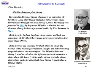
- 42. 01/05/15 42 Plate Theories Mindlin–Reissner plate theory Raymond David Mindlin (1906- 1987) Eric Reissner (1913 - 1996) The Mindlin-Reissner theory of plates is an extension of Kirchhoff–Love plate theory that takes into account shear deformations through-the-thickness of a plate. The theory was proposed in 1951 by Raymond Mindlin. A similar, but not identical, theory had been proposed earlier by Eric Reissner in 1945. Both theories are intended for thick plates in which the normal to the mid-surface remains straight but not necessarily perpendicular to the mid-surface. The Mindlin-Reissner theory is used to calculate the deformations and stresses in a plate whose thickness is of the order of one tenth the planar dimensions while the Kirchhoff-Love theory is applicable to thinner plates. Both theories include in-plane shear strains and both are extensions of Kirchhoff-Love plate theory incorporating first- order shear effects. SOLO Introduction to Elasticity
- 43. 01/05/15 43 Mindlin–Reissner plate theoryKirchhoff–Love plate theory Equilibrium equations Constitutive relations Therefore the only non-zero strains are in the in-plane directions. Unlike Kirchhoff-Love plate theory where are directly related to , Mindlin's theory requires that SOLO Deformed Midsurface Original Midsurface Deformed Midsurface Original Midsurface x w y w yx ∂ ∂ −= ∂ ∂ = θθ , wuz y w zuz x w zu zxyyx =−= ∂ ∂ −== ∂ ∂ −= ,, θθ wuz y w zuz x w zu zxyyx =−= ∂ ∂ −== ∂ ∂ −= ,, θθ x w y w yx ∂ ∂ −≠ ∂ ∂ ≠ θθ , ( ) + −− −− = xy yy xx xy yy xx E EE EE γ ε ε ν νν ν ν ν ν σ σ σ 12 00 0 11 0 11 22 22 yx w kkz yx w z x u y u y w kkz y w z y u x w kkz x w z x u xyxy yx xy yyyy y yy xxxx x xx ∂∂ ∂ =−= ∂∂ ∂ −= ∂ ∂ + ∂ ∂ = ∂ ∂ =−= ∂ ∂ −= ∂ ∂ = ∂ ∂ =−= ∂ ∂ −= ∂ ∂ = 22 2 2 2 2 2 2 2 2 :,22 :, :, γ ε ε 0=== zzyzxz εγγ 0,0, =≠ zzyzxz εγγ ( ) ( ) ( ) + + + −− −− = yz xz xy yy xx yz xz xy yy xx E E E EE EE γ γ γ ε ε ν ν ν νν ν ν ν ν σ σ σ σ σ 12 0000 12 000 00 12 00 000 11 000 11 22 22
- 44. 01/05/15 44 Mindlin–Reissner plate theory Constitutive relations SOLO
- 45. 01/05/15 Mindlin–Reissner plate theory Governing equations Relationship to Reissner theory Reissner's theory Mindlin's theory SOLO Return to Table of Content
- 46. 46 Let consider an arbitrary Membrane Surface Element Δ S, encompassed by a closed curve γ, and its projection on x-y plane is the Surface Element Δ A. A Membrane is an Elastic Skin (h <<L) which does not resist bending (zero shear)but does resist stretching. We assume that such a Membrane is stretched over a certain simple connected planar region R (x-y plane) bounded by a rectifiable curve C. We assume a constant tension τ on the boundary curve, normal to C in the Membrane plane. Let be the parametric representation of γ, where s stands for the arc length on γ. ( ) ( ) ( ),,,: suusyysxx ===γ ( ) ( ) ( )[ ] 2/1222 zdydxdsd ++= The Membrane is represented by u = u (x,y,t) at any time t. If we define ( ) ( ) 0,,:,,, =−=Φ utyxutuyx and ( ) k u u j y u i x u tuyxn ∂ ∂ − ∂ ∂ + ∂ ∂ =Φ∇= ,,, a vector orthogonal to ΔS. 1 222 = ∂ ∂ + ∂ ∂ + ∂ ∂ = ∂ ∂ + ∂ ∂ + ∂ ∂ = s u s y s x tk s u j s y i s x t a vector tangent to γ. SOLO Introduction to Elasticity Membrane Theory
- 47. 01/05/15 47 ( ) n tn P × =ττthen 11 ,, 1, 22 << ≈++= ∂ ∂ = ∂ ∂ =−+= yx uu yx yxyx uun y u u x u ukjuiun ( ) ∂ ∂ − ∂ ∂ + + ∂ ∂ − + ∂ ∂ ≈− ∂ ∂ ∂ ∂ ++ = k sd xd y u sd yd x u j sd xd sd zd x u i sd yd sd zd y u sd zd sd yd sd xd y u x u kji uu yx P τ τ τ 1 1 22 ( ) kji uyxP ττττ ++= Let derive the External Force executed on the surface ΔS in direction.k ( ) ∫∫∫∫∫∑ ∆ ∂ ∂ + ∂ ∂ = ∂ ∂ − ∂ ∂ = ∂ ∂ − ∂ ∂ ==∆ A ThsGreen u ydxd y u x u kxd y u yd x u kksd sd xd y u sd yd x u ksdkS 2 2 2 2.' τττττ γγγ Since we obtain applying the Mean Value TheoremAydxd A ∆=∫∫∆ ( ) ( ) ( ) AyxA y u x u kkS ∆∈==∆ ∂ ∂ + ∂ ∂ =∆∑ ηξττ ηξ , , 2 2 2 2 22 1 yx uu S n S A ++ ∆ = ∆ =∆ τ is the external tension on the Membrane Boundary SOLO Introduction to Elasticity Membrane Theory
- 48. 01/05/15 48 Membrane Theory If ρ is the constant density of the Surface Element ΔS of the Membrane, then the mass is ρ ΔS, and we have ( ) ( ) ( ) ( ) AyxkA t u kydxduu t u k t u S A yx ∆∈==∆ ∂ ∂ ≈ ++ ∂ ∂ = ∂ ∂ ∆ ∫∫∆ ηξρ ρρ ηξ ηξηξ , 1 , 2 2 22 , 2 2 , 2 2 We have ( ) ( ) k t u SkSfkS ηξ ρτ , 2 2 ∂ ∂ ∆=∆+∆∑ therefore ( ) ( ) A t u Af y u x u ∆ ∂ ∂ =∆ + ∂ ∂ + ∂ ∂ ηξηξ ρτ , 2 2 , 2 2 2 2 We can cancel by ΔA and by shrinking it than ( ) ( ) ( ) ( )yxyx ,,&,, →→ ηξηξ ( ) ρρ τ yxtf y u x u t u ,, 2 2 2 2 2 2 + ∂ ∂ + ∂ ∂ = ∂ ∂ Membrane Equation f – force per unit surface normal to Membrane [N/m2 ] SOLO Introduction to Elasticity Return to Table of Content
- 49. SOLO Introduction to Elasticity Vibration The Elastic Energy of a Body: [ ] [ ] [ ] [ ] ∫∫∫∫∫∫∫∫∫ === V TTT V T V T VduBCBuVduBuBCVdU 3x66x66x33x63x66x6 2 1 2 1~~ 2 1 εσ [ ] ( ) [ ]εσ ~,,~ 6x6 zyxC= [ ] u z y x u u u zyx zyxB ∂ ∂ ∂ ∂ ∂ ∂ = ,,,,,~ 3x6ε [ ] [ ] [ ] [ ]yzxzxyzzyyxx T yzxzxyzzyyxx T εεεεεεεσσσσσσσ == :~,:~ =≠=+= ∂ ∂ + ∂ ∂ = == ∂ ∂ = zyxjijiuu x u x u zyxiu x u jiijji i j j i ij ii i i ii ,,,: ,,: ,, , εε ε
- 50. SOLO Introduction to Elasticity The Virtual Work done by external forces: ( ) ( ) ( ) ( ) ( ) ( )∫∫∫ ∑∫∫ ∫∫ ⋅+ −−−⋅+ ⋅= V B i S iiii S zdydxdtzyxuf zdydxdzzyyxxtzyxuF ydxdtzyxuqW ,,, ,,, ,,, δδδ The Kinetic Energy: ( ) ( ) ∫∫∫ ∂ ∂ ⋅ ∂ ∂ = V zdydxd t tzyxu t tzyxu K ρ ,,,,,, 2 1 The Total Energy Function: ( ) ( ) ( ) ( ) ( ) ( ) ( ) ( )∫∫∫ ∑ ∫∫∫∫ ∫∫∫∫∫∫ ⋅+ −−−⋅+⋅+ − ∂ ∂ ⋅ ∂ ∂ =+−= V B i S iiii S V TT V zdydxdtzyxuf zdydxdzzyyxxtzyxuFydxdtzyxuq zdydxduBCBuzdydxd t tzyxu t tzyxu WUTL ,,, ,,,,,, 2 1,,,,,, 2 1 δδδ ρ – displacement [m] – force per unit surface S [N/m2 ] – force per unit volume [N/m3 ] – discrete forces [N], i=1,2,…,mi B F f q u Vibration
- 51. SOLO Introduction to Elasticity The Lagrangian: ( ) ∫∫∫∫∫ == 2 1 2 1 t t V t t tdzdydxdtdLCI L The Extremum: ( ) ( ) ( ) ( )[ ] ( ) ( ) ( ) ( ) ( )tzyxufzzyyxxtzyxuFtzyxutzyxq uBCBu t tzyxu t tzyxu B i iiii TT ,,,,,,,,,,,, 2 1,,,,,, 2 ⋅+−−−⋅+⋅∇+ − ∂ ∂ ⋅ ∂ ∂ = ∑ δδδ ρ L Vibration
- 52. SOLO Introduction to Elasticity For a Freely Vibrating System, with no external forces, the Lagrangian reduces to: ( ) ( ) uBCBu t tzyxu t tzyxu TT 2 1,,,,,, 2 − ∂ ∂ ⋅ ∂ ∂ = ρ L Euler-Lagrange Equations: 0= ∂ ∂ − ∂ ∂ ∂ ∂ u t utd d LL ( ) ( ) VintzyxuBCB t tzyxu T 0,,, ,,, 2 2 =− ∂ ∂ ρ For the Vibrating System a Separation of Variables for the Space and Time is ( ) ( ) ( )tzyxUtzyxu ωcos,,,,, = that gives ( ) ( ) VinzyxU zyx zyxBC zyx zyxBzyxU T 0,,,,,,,,,,,,,,2 = ∂ ∂ ∂ ∂ ∂ ∂ ∂ ∂ ∂ ∂ ∂ ∂ − ωρ The Boundary Condition must be included Return to Table of Content Vibration
- 53. SOLO Energy Equations for a Beam Pure Torsion Vibration ( ) ldd ργθρ = ( ) ( ) ld d GG θ ρργρτ == x L dx ( ) ld dθ ρργ = ( ) ld d JGAd ld d GAd ld d GAdFdTx θ ρ θθ ρρτρρ ===== ∫∫∫∫ 22 ∫= AdJ 2 : ρ ( ) ρ ρτ JTx = ∫∫ ∫∫ ∫∫∫ ∫∫∫ ∫∫ = = = = = = L x L L x L A x L A L A ld ld d Tld ld d JG ld JG T ldAd JG T ldAd G ldAdU 00 2 0 2 0 2 22 0 2 0 2 1 2 1 2 1 2 1 2 1 2 1 θθ ρτ τγ Introduction to Elasticity
- 54. SOLO x L dx The Kinetic Torsional Energy of the Beam of Length L ∫ ∂ ∂ = L p ld t JK 0 2 2 1 θ ρ The Total Energy of a Beam of length L is ∫ + =+= L p ld ld d J ld d JGUKE 0 22 2 1 θ ρ θ ∫∫= L r p ldAdrJ 0 0 2 1st torsional 2nd torsional The Euler-Lagrange Equation is 0= ∂ ∂ ∂ ∂ − ∂ ∂ ∂ ∂ xt td d θθ LL ∫= AdJ 2 : ρ Therefore 2 2 2 2 xJ JG t p ∂ ∂ = ∂ ∂ θ ρ θ Torsional Beam Vibration Introduction to Elasticity Pure Torsion Vibration Return to Table of Content
- 55. SOLO Energy Equations for Pure Bending Beam (2) Pure Bending ldd =θρ Q M M͛ P͛ P N N͛ Q͛ A B S R dx x y z S͛ R͛ A͛ B͛ bM M y ρ ( ) ρθρ θρθρ ε y d ddy xx = −+ = ρ εσ y EE xxxx == zxz I E Ady E AdyM ρρ σ === ∫∫∫∫ 2 2 2 ld d IE ld d IEM zzz θθ == ld d v =θ y I M z z xx =σ ( ) ( ) ∫ ∫∫∫ ∫∫ ∫∫∫ ∫∫∫ ∫∫ = = = = = = = = L L zz L z L z L z z L A z z L A xx L A xxxx Energy Potential ld ld d Mld ld d Mld ld d IEld ld d IE ld IE M ldAdy IE M ldAd E ldAdV 0 0 2 2 0 2 2 2 0 2 0 2 0 2 2 2 0 2 0 v 2 1 2 1v 2 1 2 1 2 1 2 1 2 1 2 1 θθ σ εσ ∫∫= xA z zdydyI 2 : Vibration of Euler-Bernoulli Bending Beam Introduction to Elasticity
- 56. 01/05/15 56 Finite element method model of a vibration of a wide-flange beam (I-beam). The dynamic lateral beam equation is the Euler-Lagrange equation for the following action ( ) ( ) ( ) ∫∫∫∫ + ∂ ∂ − ∂ ∂ = ∂ ∂ ∂ ∂ 2 1 2 1 0 2 2 22 2 2 0 ,v x v 2 1v 2 1 x v , v v,,, t t L xqLoadsExternal todueEnergy ForcesInternaltodue EnergyPotential z EnergyKinetic t t L tdxdtxxqIE t tdxd t xt ρL Euler-Lagrange ( ) 0 x v x v vvv 2 2 2 2 2 2 2 22 2 =− ∂ ∂ ∂ ∂ + ∂ ∂ = ∂ ∂ − ∂ ∂ ∂ ∂ ∂ ∂ − ∂ ∂ ∂ ∂ xqIE t x x t td d zρ LLL ( )xq t IE z + ∂ ∂ −= ∂ ∂ ∂ ∂ 2 2 2 2 2 2 v x v x ρ Dynamic Beam Equation SOLO Vibration of Euler-Bernoulli Bending Beam Introduction to Elasticity
- 57. 01/05/15 57 1st lateral bending1st vertical bending 2nd lateral bending2nd vertical bending http://en.wikipedia.org/wiki/Bending Dynamic Lateral Beam Equation SOLO Introduction to Elasticity
- 58. 01/05/15 58 Rayleigh Beam Model Shear Beam Model Euler-Bernoulli Beam Introduction to Elasticity
- 59. 01/05/15 59 Timoshenko Beam Model Rotating Timoshenko Beam Introduction to Elasticity Return to Table of Content
- 60. 01/05/15 60 SOLO Vibration Modes of a Free-Free Beam Introduction to Elasticity
- 61. 61 Introduction to Elasticity J - Mass Moment of Inertia (Rotary Inertia) per unit length x - Length A - Cross Section Area μ - Mass per Unit Length M - Bending Moment V - Shear Force θ - Angular Displacement v - Beam Deflection q - Force per Unit Length E - Young’s Modulus G - Shear Modulus k - Torsional Constant for A I - Centroidal Moment of Inertia SOLO Vibration Modes of a Free-Free Beam (continue - 1)
- 62. 62 ( )xtq x V t , v 2 2 = ∂ ∂ + ∂ ∂ µ Summing the Vertical Forces and Moments acting on the Beam Element 02 2 = ∂ ∂ − ∂ ∂ + x M t JV θ From Elementary Beam Theory: ∂ ∂ −= ∂ ∂ = x GKV x IEM v θ θ Introduction to Elasticity ( ) 2 2 v , t xdxd x V VVxdxtq ∂ ∂ = ∂ ∂ +−+ µ 2 2 t xdJxd x M MMxdxd x V V ∂ ∂ = ∂ ∂ +−+ ∂ ∂ +− θ SOLO Vibration Modes of a Free-Free Beam (continue - 2)
- 63. 63 Introduction to Elasticity xx GKV GK finiteV ∂ ∂ = ∂ ∂ −= → ∞→ vv θθ x M V x M t JV J ∂ ∂ =→ ∂ ∂ + ∂ ∂ −= =0 2 2 θ q x IE xt q x V t xx IEM x M V = ∂ ∂ ∂ ∂ + ∂ ∂ →= ∂ ∂ + ∂ ∂ ∂ ∂ ∂ ∂ = ∂ ∂ = 2 2 2 2 2 2 v 2 2 vvv µµ q x IE t = ∂ ∂ + ∂ ∂ 4 4 2 2 vv µ 0& =∞→ JGKFor a Slender Beam For a Homogeneous Beam (E I = constant) SOLO Vibration Modes of a Free-Free Beam (continue - 3)
- 64. 64 Introduction to Elasticity Free Vibration of an Uniform Beam Assume Free-Free case when the Shear and Bending Moment at the ends of the Beam are Zero. 0 vv 4 4 2 2 = ∂ ∂ + ∂ ∂ x IE t µ Assume Separation of Variables ( ) ( ) ( )tTxtx φ=,v . 1 2 4 42 const td dIE td Td T ===− ω φ φµ Then we can write SOLO Vibration Modes of a Free-Free Beam (continue - 4)
- 65. 65 Introduction to Elasticity =− =+ 0 0 2 4 4 2 2 φωµ φ ω td d IE T td Td ( ) ( ) = = → ∂ ∂ ∂ ∂ = ∂ ∂ = = = = = 0 0 v 2 2 0 2 2 00 0 Lx x M LM xd d xd d xx IE x IEM φ φ θ ( ) ( ) = = → ∂ ∂ = ∂ ∂ = = = = = 0 0 v 3 3 0 3 3 00 03 3 Lx x V LV xd d xd d x IE x M V φ φ with the Boundary Conditions: - represents the shape of a Natural Vibration Modeϕ ω - is the Vibration Frequency corresponding to this Mode. SOLO Vibration Modes of a Free-Free Beam (continue - 5)
- 66. 66 ( )La/cosh 1 ω ( )La/cos ω La/ω π 2 7 π 2 5 π51.1 0 Introduction to Elasticity The General Solution of the Equations: =− =+ 0 0 2 4 4 2 2 φωµ φ ω td d IE T td Td ( ) ( ) ( ) ( ) +++ − − = += LLLL LL LL Cl tCtCtT ii iiiii γγγγ γγ γγ φ ωω coshcossinsinh sinsinh coshcos cossin 4 21 m IE a a i == :&: 22 ω γ is where To satisfy the Boundary Conditions ω is such that: i.e., only Discrete Values ωi, i=0,1,2…., of ωi called Modes are acceptable solutions ,2,1,01coshcos 2/12/1 == iL a L a ii ωω SOLO Vibration Modes of a Free-Free Beam (continue - 6)
- 67. 67 ( )La/cosh 1 ω ( )La/cos ω La/ω π 2 7 π 2 5 π51.1 0 Rigid-Body Mode ( i = 0 ) First Mode ( i = 1 ) Second Mode ( i = 2 ) Third Mode ( i = 3 ) For a Circular Cross-Section Area of Diameter D Decreases as the Length L Increases and Diameter D Decreases. Introduction to ElasticitySOLO Vibration Modes of a Free-Free Beam (continue - 7)
- 68. 68 Rigid-BodeMode n=0 Fi n=1 SecondMode n=2 ThirdMode n=3 ( ) ( ) mIEL //2/5 222 2 πω = ( ) ( ) mIEL //2/7 222 3 πω = ( ) ( ) mIEL //51.1 222 1 πω = 00 =ω L l The Complete Solution for the Elastic Motion in Case of Free Vibrations is: It can be shown that the Modes satisfy: i.e, every two Distinct Modes are Orthogonal. Introduction to ElasticitySOLO Vibration Modes of a Free-Free Beam (continue - 8)
- 69. 69 Introduction to Elasticity First 5 Mode Shape for a Free-Free Beam SOLO Vibration Modes of a Free-Free Beam (continue - 9)
- 70. 70 FORCED VIBRATIONS When Forces are applied Normal to the Beam, we have: Consider the General Solution: Where are the Modes of the Free-Free case If we substitute the general Solution in the previous Differential Equation, multiply by and integrate over the Length, we obtain Introduction to ElasticitySOLO Vibration Modes of a Free-Free Beam (continue - 10)
- 71. 71 ELASTIC MODES OF A MISSILE SOLO1 Using the Orthogonality of the Modes , we obtain: or where In order to account for the Structural Damping we rewrite the Differential Equation as follows : IS THE GENERALIZED MASS IS THE GENERALIZED FORCE Introduction to ElasticitySOLO Return to Table of Content Vibration Modes of a Free-Free Beam (continue - 11)
- 72. 01/05/15 72 SOLO Deformation Energy The Virtual Work due to External Loads q [N/m2 ] and Discrete Forces Fi [N] is Vibration of Kirchhoff Plate (Classical Plate Theory) ( ) ( ) ( ) ( ) ( ) ydxd yx w y w x w y w y w x w x whE ydxdzdz yx w y w x w y w y w x w x wE ydxdzd y w z y w x w z yx w z x w z y w x w z E zdydxdzdydxdU S h hS S h h V yyyyxyxyxxxx V T ∫∫ ∫∫∫ ∫∫ ∫ ∫∫∫∫∫∫ ∂∂ ∂ −+ ∂ ∂ + ∂ ∂ ∂ ∂ + ∂ ∂ + ∂ ∂ ∂ ∂ − = ∂∂ ∂ −+ ∂ ∂ + ∂ ∂ ∂ ∂ + ∂ ∂ + ∂ ∂ ∂ ∂ − = ∂ ∂ − ∂ ∂ + ∂ ∂ − ∂∂ ∂ −+ ∂ ∂ − ∂ ∂ + ∂ ∂ − − = ++== + − + − 22 2 2 2 2 2 2 2 2 2 2 2 2 2 3 2/ 2/ 2 22 2 2 2 2 2 2 2 2 2 2 2 2 2 2/ 2/ 2 2 2 2 2 222 2 2 2 2 2 2 2 2 12 1122 1 12 12 1 12 12 1 2 2 1~~ 2 1 ννν ν ννν ν ννν ν εσγσεσεσ ( ) ( ) ( ) ( ) ydxdyyxxtyxwFydxdtyxwqW i S iii S ∑∫∫∫∫ −−+= δδ,,,, Kinetic Energy ( ) ∫∫ ∂ ∂ = S ydxd t tyxwh K ρ 2 ,, 2 Total Energy ( ) ( ) ( ) ( ) ( ) ( ) ( )∑ ∫∫∫∫ ∫∫∫∫ −−++ ∂∂ ∂ −+ ∂ ∂ + ∂ ∂ ∂ ∂ + ∂ ∂ + ∂ ∂ ∂ ∂ − − ∂ ∂ =+−= i S iii S S D S ydxdyyxxtyxwFydxdtyxwq ydxd yx w y w x w y w y w x w x whE ydxd t tyxwh WUKL δδ ννν ν ρ ,,,, 12 1122 1,, 2 22 2 2 2 2 2 2 2 2 2 2 2 2 2 32 Introduction to Elasticity
- 73. SOLO ( ) ( ) ( ) ( ) ( ) ( ) ( ) ∫∫∫∑ ∫∫∫∫∫∫ ∫∫∫∫∫∫∫ =−−++ ∂∂ ∂ −+ ∂ ∂ + ∂ ∂ ∂ ∂ + ∂ ∂ + ∂ ∂ ∂ ∂ − ∂ ∂ = 2 1 2 1 2 1 2 1 2 1 2 1 ,,,,,, 12 2 1,, 2 22 2 2 2 2 2 2 2 2 2 2 2 22 t t Si t t S iii t t S t t S t t S t t tdydxdtdydxdyyxxtyxwFtdydxdtyxwtyxq tdydxd yx w y w x w y w y w x w x w Dtdydxd t tyxwh tdL Lδδ νννρ Euler-Lagrange: 02 2 2 22 2 2 22 2 = ∂ ∂ − ∂∂ ∂ ∂ ∂ ∂∂ ∂ −− ∂ ∂ ∂ ∂ ∂ ∂ − ∂ ∂ ∂ ∂ ∂ ∂ − ∂ ∂ ∂ ∂ w yx wyx y wy x wx t wtd d LLLLL ( ) ( ) ( )∑ −−++ ∂∂ ∂ ∂∂ ∂ −+ ∂ ∂ + ∂ ∂ + ∂ ∂ + ∂ ∂ ∂ ∂ + ∂ ∂ + ∂ ∂ + ∂ ∂ + ∂ ∂ ∂ ∂ − ∂ ∂ i iii yyxxFq yx w yxx w y w y w x w yy w x w y w x w x D t w h δδ νννννρ 22 2 2 2 2 2 2 2 2 2 2 2 2 2 2 2 2 2 2 2 2 2 2 14 2 1 ( ) ( ) 02 2 2 2 2 2 2 2 2 2 =−−++ ∂ ∂ + ∂ ∂ ∂ ∂ + ∂ ∂ − ∂ ∂ ∑i iii yyxxFq y w x w yx D t w h δδρ Plate Vibration Equation ( ) ( ) 02 4 4 22 4 4 4 2 2 =−−++ ∂ ∂ + ∂∂ ∂ + ∂ ∂ − ∂ ∂ = ∑i iii yyxxFq y w yx w x w D t w h δδρ ( ) ( ) ( ) ( ) ( ) ( ) ( )∑ −−++ ∂∂ ∂ −+ ∂ ∂ + ∂ ∂ ∂ ∂ + ∂ ∂ + ∂ ∂ ∂ ∂ − ∂ ∂ = i iii yyxxtyxwFtyxwtyxq yx w y w x w y w y w x w x w D t tyxwh δδ ννν ρ ,,,,,, 12 2 1,, 2 : 22 2 2 2 2 2 2 2 2 2 2 2 22 L Vibration of Kirchhoff Plate (Classical Plate Theory) Introduction to Elasticity
- 74. Vibration of Rectangular Plate SOLO 2 2 4 4 2 2 2 2 4 4 4 2 2 t w D h y w y w x w x w w ∂ ∂ −= ∂ ∂ + ∂ ∂ ∂ ∂ + ∂ ∂ =∇ ρ Consider a rectangular plate which has dimensions a x b in the (x,y) -plane and thickness 2hin the w direction. We seek to find the free vibration modes of the plate. Separation of variables ( ) ( ) ( )tTyxWtyxw ,,, = 2 2 2 4 4 2 2 2 2 4 4 1 2 2 ω ρ =−= ++ td Td Tyd Wd yd Wd xd Wd xd Wd Wh D D h WW D h yd Wd yd Wd xd Wd xd Wd ρ ωλλ ωρ 2 : 2 2 24 2 4 4 2 2 2 2 4 4 ===++ ( ) b xn a xm yxW ππ sinsin, = Assume a Rectangular Plate with clamped circumference, than the boundary conditions are ( ) byat y w x w DM axat y w x w DM byandaxattyxwCB yy xx ,00 ,00 ,0,00,,:.. 2 2 2 2 2 2 2 2 == ∂ ∂ + ∂ ∂ = == ∂ ∂ + ∂ ∂ = === ν ν Since the above equation is a biharmonic eigenvalue problem, we look for Fourier expansion solutions of the form Introduction to Elasticity
- 75. Vibration of Rectangular Plate (continue -1) SOLO ( ) b xn a xm yxW ππ sinsin, = Substituting the solution into the biharmonic equation gives us ( ) ( ) ( ) ( ) 0,0,,,0 ======== byxWyxWyaxWyxW ( ) ( ) b xn a xm b m yx yd Wd b xn a xm a m yx xd Wd ππππππ sinsin,,sinsin, 2 2 22 2 2 −= −= ( ) ( ) b xn a xm b m yx yd Wd b xn a xm a m yx xd Wd ππππππ sinsin,,sinsin, 4 4 44 4 4 = = b xn a xm b xn a xm b m b m a m a m yd Wd yd Wd xd Wd xd Wd ππ λ ππ π sinsinsinsin22 4 4224 4 4 4 2 2 2 2 4 4 = + + =++ We can see that We can see also that ( ) ( ) byattT yd Wd xd Wd DMaxattT yd Wd xd Wd DM yyxx ,00&,00 2 2 2 2 2 2 2 2 == +=== += νν + = 22 22 b m a m πλ ,2,1, 22 22 22 = + == nm b m a m h D h D mn ρ π ρ λω Therefore the general solution for the plate equation is ( ) ( ) ( )( )∑∑ ∞ = ∞ = += 1 1 cossinsinsin, m n mnmnmnmn tBtA b xn a xm yxw ωω ππ Introduction to Elasticity Return to Table of Content
- 76. Vibration of Cylindrical Plate SOLO The governing equation for free vibrations of a circular plate of thickness 2h is 2 2 4 21 t w D h r w r r r r r rr w ∂ ∂ −= ∂ ∂ ∂ ∂ ∂ ∂ ∂ ∂ =∇ ρ Expanded to 2 2 32 2 23 3 4 4 2112 t w D h r w rr w rr w rr w ∂ ∂ −= ∂ ∂ + ∂ ∂ − ∂ ∂ + ∂ ∂ ρ Separation of variables ( ) ( ) ( )tTrRtrw =, constant td Td Trd Rd rrd Rd rrd Rd rrd Rd R ==−= +−+ 2 2 2 32 2 23 3 4 4 11121 ω β D hρ β 2 := 02 2 2 =+ T td Td ω ( ) ( ) ( )tBtAtT ωω sincos += R rd Rd rrd Rd rrd Rd rrd Rd 4 2 32 2 23 3 4 4 112 λ ωβ=+−+ where J0 is the order 0 Bessel Function of the First Kind and I0 is the order 0 Modified Bessel Function of the First Kind. ( ) ( ) ( )rIDrJCrR λλ 00 += ( ) ( ) 0&0:.. = = == rd arRd arRCB The constants C1 and C2 are determined from the boundary conditions. For a plate of radius with a clamped circumference, the boundary conditions are Introduction to Elasticity
- 77. Vibration of Cylindrical Plate (continue – 1) SOLO From these boundary conditions we find that ( ) ( ) ( ) ( ) 01010 =+ aJaIaIaJ λλλλ We can solve this equation for λn (and there are an infinite number of roots) and from that find the modal frequencies . We can also express the displacement in the form ( ) ( ) ( ) ( ) ( ) ( ) ( ) ( ) ( )[ ]∑ ∞ = + −== 1 0 0 0 0 cossin, n nnnnn n n nn tBtArI aI aJ rJCtTrRtrw ωωλ λ λ λ For a given frequency ωn the first term inside the sum in the above equation gives the mode shape. mode n = 1 mode n = 2 http://en.wikipedia.org/wiki/Vibration_of_plates Introduction to Elasticity Return to Table of Content
- 78. 01/05/15 78 http://en.wikipedia.org/wiki/Vibrations_of_a_circular_membran SOLO Vibrations of a Circular Membrane ∂ ∂ + ∂ ∂ = ∂ ∂ 2 2 2 2 2 2 y u x u t u ρ τ ( ) 0,,:.. 20,0,: 11 2 2 2 22 2 2 2 2 == ≤≤≤≤= ∂ ∂ + ∂ ∂ + ∂ ∂ = ∂ ∂ taruCB arc u rr u rr u c t u θ πθ ρ τ θ Polar θ θ sin cos ry rx = = Separation of Variables ( ) ( ) ( ) ( )tTrRtru θθ Θ=,, ( ) ( ) ( ) ( ) ( ) ( ) ( ) ( ) 2 22 "'"" λ θ θ −= Θ Θ ++= rrRr rR rR rR tTc tT ( ) ( ) ( ) ( ) ( ) ( ) Lr rR rR r rR rR r = Θ Θ −=++ θ θ λ "'" 222 ( ) ( ) ( ) ,2,1sincos =+=Θ mmDmC θθθ ( ) ( ) 0" 2 =Θ+Θ θθ m 2 mL = ( ) ( ) ( )[ ] ( ) ( ) ( )[ ]θθλλλθ mDmCrJtcBtcAtru mnmmnmnmn sincossincos,, ++= ( ) ( ) ,2,1, == nmrJrR mnm λ Bessel Function ( ) ( ) 0" 22 =+ tTctT λ ( ) ( ) ( )tcBtcAtT λλ sincos += ( ) ( ) ( ) ( ) ( ) ( ) 2 2 "'" λ θ θ −= Θ Θ ++ rrRr rR rR rR Introduction to Elasticity
- 79. 01/05/15 79 http://en.wikipedia.org/wiki/Vibrations_of_a_circular_membran Mode u01 (1s) with Mode u02 (2s) with Mode u03 (3s) with Mode u11 (2p) with Mode u12 (3p) with Mode u13 (4p) with Mode u21 (3d) with Mode u22 (4d) with Mode u23 (5d) with Modes of Vibration of a Circular Membrane SOLO ( ) ( ) ( )[ ] ( ) ( ) ( )[ ]θθλλλθ mDmCrJtcBtcAtru mnmmnmnmn sincossincos,, ++= Introduction to Elasticity Return to Table of Content
- 80. 01/05/15 80 Numerical Methods in Elasticity SOLO Introduction to Elasticity Problems in Physics and in Engineering (including Elasticity) are often described by Differential Equations, together with related Boundary Conditions and initial Conditions. For some of those problems there exists Extremum Principles, by which the solutions must make an appropriate functional stationary, or, in certain cases, even extremal. In those cases Variational Methods can be used that reduce to Euler-Lagrange Differential Equations. There are also problems for which no Extremum Principles can be derived, and we must start with the Differential Equations derived from the Physics of the problem. To solve the problems with Extremum Principles and others we must solve Differential equations. This is done, in general, using Numerical Methods Return to Table of Content
- 81. 01/05/15 81 John William Strutt, 3rd Baron Rayleigh, (1842 – 1919) Lord Rayleigh published in the “Philosophical Transactions of the Royal Society”, London, A, 161, 77 (1870) that the Potential and Kinetic Energies in an Elastic System are distributed such that the frequencies (eigenvalues) of the components are a minimum. His discovery is now called the “Rayleigh Principle” The Potential and Kinetic Energies of a discrete Elastic System of n degrees of freedom are given by [ ] [ ] xmxT xkxV T T 2 1 2 1 = = The Total Energy is [ ] [ ] xmxxkxTVE TT 2 1 2 1 +=+= For a Conservative System the Total Energy is constant. In this case when the Potential Energy is Maximal, V = Vmax, than T = 0, and when the Kinetic Energy is Maximal, K = Kmax than V = 0, therefore ETV == maxmax Rayleigh Principle SOLO Introduction to Elasticity Rayleigh–Ritz Method
- 82. 01/05/15 82 John William Strutt, 3rd Baron Rayleigh, (1842 – 1919) To find the natural modes (frequencies) we assume a harmonic motion tXx ωcos = By substituting the harmonic motion in Vmax, and Kmax we find Rayleigh Principle (continue – 1) where denotes the vector of amplitudes (mode shape) and ω represents the natural frequency of vibration. X [ ] [ ] ( ) ,1,0 2 12 2 1 ,1,0 2 1 2 max max =+== === mmtXmXT mmtXkXV T T π ωω πω By equating the mean values of Vmax, and Kmax we obtain [ ] [ ] XmX XkX T T =2 ω The right side of this expression is denoted by ( ) [ ] [ ] QuotientsRayleigh XmX XkX XR T T ': = SOLO Introduction to Elasticity
- 83. 01/05/15 83 John William Strutt, 3rd Baron Rayleigh, (1842 – 1919) Assume that are the Normalized Modes of (Amplitudes and Frequencies) of the System (that satisfy System Boundary Conditions) such that ,2,1, =iX ii ω Rayleigh Principle (continue – 2) [ ] [ ] [ ] [ ] [ ] [ ] [ ] [ ] +++= +++= 33 2 322 2 211 2 1 33 2 322 2 211 2 1 XmXcXmXcXmXcXmX XkXcXkXcXkXcXkX TTTT TTTT and [ ] [ ] [ ] ijij T iij T i ijj T i XmXXkX ji ji XmX δωω δ 22 0 1 == ≠ = == Then for any harmonic we can writetXx ωcos = ( )XXcXcXcXcXcX T iiii =+++++= 332211 ( ) [ ] [ ] [ ] [ ] [ ] [ ] [ ] [ ] [ ] [ ] [ ] [ ] [ ] [ ] +++ +++ = +++ +++ === 33 2 322 2 211 2 1 33 2 3 2 322 2 2 2 211 2 1 2 1 33 2 322 2 211 2 1 33 2 322 2 211 2 12 : XmXcXmXcXmXc XmXcXmXcXmXc XmXcXmXcXmXc XkXcXkXcXkXc XmX XkX XR TTT TTT TTT TTT T T ωωω ω ( ) ( ) ( ) ( ) ( ) ( ) ( ) +++ +++ = +++ +++ == 2 3 2 2 2 1 2 3 2 3 2 2 2 2 2 1 2 1 2 3 2 2 2 1 2 3 2 3 2 2 2 2 2 1 2 12 : XXXXXX XXXXXX ccc ccc XR TTT TTT ωωωωωω ω or SOLO Introduction to Elasticity
- 84. 84 John William Strutt, 3rd Baron Rayleigh, (1842 – 1919) Assume that ( ) 22 εδδ ≤+= ∑i r T irr XXXXX Rayleigh Principle (continue – 2) ( ) ( )[ ] ( )[ ] ( )[ ] ( )[ ] [ ] [ ] ( )[ ]22 1 2 2 1 222 2 1 2 2 2 1 2 2 01 21 2 εω δδ ωδωδω δδ ωδωδ δ +≈ ++ ++ = +++ +++ =+= ∑ ∑ ∑ ∑ ∞ = ∞ = ∞ ≠ = ∞ ≠ = r r T r i i T r rr T r i ii T rr r T rr ri i i T rr rr T rr ri i ii T rr rr XXXX XXXX XXXXXX XXXXXX XXXR where 0 (ε2 ) represents an expression in ε of the second order or higher. differs from the eigenvector by a small quantity of the first order, and satisfies all the System Boundary Conditions. X rX rX 01/05/15 Suppose that ωmin and ωmax are the minimum and maximum of the System Frequencies Modes: ωmin ≤ ωi ≤ ωmax i=1,2,… , then ( ) ( ) 2 max 2 3 2 2 2 1 2 3 2 3 2 2 2 2 2 1 2 1 2 min 2 3 2 2 2 1 ωωωωω +++≤+++≤+++ ccccccccc Therefore ( ) 2 max2 3 2 2 2 1 2 3 2 3 2 2 2 2 2 1 2 12 min ω ωωω ω ≤ +++ +++ =≤ ccc ccc XR This expression indicates that if an arbitrary vector differs from the eigenvector by a small quantity of the first order , differs from the eigenvalue ωr 2 by a small quantity of the second order. This means that the Rayleigh quotient has a stationary value in the neighborhood of an eigenvector. X rX ( )XR SOLO Introduction to Elasticity
- 85. 01/05/15 85 John William Strutt, 3rd Baron Rayleigh, (1842 – 1919) Rayleigh Principle (continue – 3) Example: A Simple Supported Beam Consider the free vibration of a simply supported uniform thin beam having flexural rigidity EI, mass per unit length m and length L Let the lateral dynamic displacement be u (x,t)= f(x) sin(wt+a). The maximum total potential energy of the vibrating beam ( )( )∫= L xdxf IE V 0 2 max " 2 The maximum velocity is w f(x). Therefore the maximum kinetic energy due to vibration ( )( )∫= L xdxfT 0 22 max 2 µ ω The admissibility conditions are that the displacement must be zero at the two supports. i.e. f(0) =0 and f(L) = 0. SOLO Introduction to Elasticity
- 86. 01/05/15 86 John William Strutt, 3rd Baron Rayleigh, (1842 – 1919) Rayleigh Principle (continue – 4) Example (continue – 1): A Simple Supported Beam ( )( ) ( )( )∫∫ = LL xdxfxdxf IE 0 22 0 2 2 " 2 µ ω From Rayleigh’s principle Tmax = Vmax gives an upper-bound estimate of the fundamental natural frequency if an admissible function is used for f(x). Therefore ( )( ) ( )( )∫ ∫ = L L xdxf xdxf IE 0 2 0 2 2 2 " 2 µ ω Using the exact fundamental mode function sin (px/L) for f(x) into the Rayleigh Quotient gives µ π ω IE L = 2 2 which is the exact value SOLO Introduction to Elasticity
- 87. 01/05/15 87 John William Strutt, 3rd Baron Rayleigh, (1842 – 1919) Rayleigh Principle (continue – 5) Example (continue – 2): A Simple Supported Beam µ ω IE L = 2 95.10 Any other admissible function for f results in a higher value for the frequency. In this case the admissibility conditions are that the displacement must be zero at the two supports. i.e. f(0) =0 and f(L) = 0. f(x) = G (x/L)(1- (x/L)) is also admissible. Substituting this into the Rayleigh Quotient equation This is about 11% higher than the exact value. SOLO Introduction to Elasticity Return to Table of Content
- 88. 01/05/15 88 Walther Ritz (1878 – 1909) John William Strutt, 3rd Baron Rayleigh, (1842 – 1919) It was observed earlier that the natural frequency calculations based on the application of Rayleigh’s principle are sensitive to the assumed displacement form, and that only one frequency can be determined. An extension of Rayleigh’s principle, which enables us to determine the higher frequencies also, is the Rayleigh-Ritz method. This method was proposed by Walter Ritz in his paper “Ueber eine neue Methode zur Loesung gewisser Variationsprobleme der Mathematishen Physik” , ]“On a new method for the solution of certain variational problems of mathematical physics”], Journal für reine und angewandte Mathematik vol. 135 pp. 1 - 61 (1909). Rayleigh–Ritz Method SOLO Introduction to Elasticity Ritz method is intended to find an approximate (numerical) solution which makes a given functional stationary. In a two dimensional region G let find a function u (x,y), subjected to given Boundary Conditions that makes a certain functional ( ) ( )∫∫∫ ∂∂ ∂ ∂ ∂ ∂ ∂ ∂ ∂ ∂ ∂ = 2 1 ,,,,,,,, 2 2 2 2 2t t V tdydxdqt yx u y u x u y u x u yxuCI L stationary. Ritz Method
- 89. 89 Walther Ritz (1878 – 1909) Ritz Method SOLO Introduction to Elasticity In order to obtain a solution Ritz proposed to choose a Set of Complete Linearly Independent Functions ( ) ( ) ( ) ( )yxyxyxyx m ,,,,,,;, 210 φφφφ The function ϕ0(x,y) is such that satisfies the Inhomogeneous Boundary Conditions. The other functions ϕ1(x,y) ,…, ϕm(x,y) must be a Complete Linearly Independent Functions that satisfy the given Homogeneous Boundary Conditions. The functions ϕ1(x,y) ,…, ϕm(x,y) are Linearly Independent Functions if ( ) ( ) ( ) 00,,, 212211 ====⇔=+++ mmm yxyxyx αααφαφαφα The functions ϕ1(x,y) ,…, ϕm(x,y) are Complete if given any function u (x,y), for any small positive quantity ε, we can find a number N and coefficients αi such that ( ) ( ) εφα <− ∑= N i ii yxyxu 1 ,,
- 90. 90 Walther Ritz (1878 – 1909) Ritz Method SOLO Introduction to Elasticity The desired function u(x,y) is expressed as a linear combination of the functions ϕ0(x,y) , ϕ1(x,y) ,…, ϕm(x,y) ( ) ( ) ( )∑= += m k kk yxcyxyxu 1 0 ,,, φφ where ck (k=1,2,…,m) are coefficients that are defined such that I (C) is stationary ( ) mk c uI k ,,2,10 == ∂ ∂ We obtain m equations with m unknowns, to obtain the coefficients ck (k=1,2,…,m) such that I (C) is stationary.
- 91. 91 Walther Ritz (1878 – 1909) Ritz Method SOLO Introduction to Elasticity Example Given a simply supported beam (1D Problem) with a concentrated load P at x = L/2. Let use ( ) ( ) = = L x x L x x π φ π φ 3 sin,sin 21 Boundary Conditions: ( ) ( ) 0,;0,0 ==== tLxutxu ( ) 00 =xφSince the there are no Inhomogeneous constraints: ( ) ( ) ( ) + =+= L x c L x cxcxcxu ππ φφ 3 sinsin 212211 The Total Static Energy is ( )2/ 2 0 2 2 2 LxuPxd xd udIE WUF L =− =−= ∫ E = Modulus of Elasticity, I = Transversal Beam Area Moment of Inertia Substituting the displacement approximation we obtain ∫ + − + =−= L ccPxd L x L c L x L c IE WUF 0 21 22 2 2 1 2 3 sin 2 sin 3 sin 3 sin 2 ππππππ Boundary Conditions are satisfied ( ) ( ) 0,;0,0 ==== tLxutxu
- 92. 92 Walther Ritz (1878 – 1909) Ritz Method SOLO Introduction to Elasticity Example (continue – 1) Integrating this equation, tacking in account the orthogonality condition ( )21 0 2 4 21 2 4 2 2 2 4 2 1 3 sinsin32 3 sin 3 sin 2 ccP xd L x L x L cc L x L c L x L c IE F L −− + + = ∫ πππππππ ≠ = =∫ nm nmL xd L xn L xm L 0 2/ sinsin 0 ππ ( )21 4 2 2 4 2 1 2 3 22 ccP L L c L L c IE F −− + = ππ we obtain To obtain a stationary F we must have 0 2 3 2 2 0 2 2 2 4 2 2 4 1 1 =+ = ∂ ∂ =− = ∂ ∂ P L L c IE c F P L L c IE c F π π 44 3 2 4 3 1 3 12 2 π π L IE P c L IE P c −= =
- 93. 93 Walther Ritz (1878 – 1909) Ritz Method SOLO Introduction to Elasticity Example (continue – 2) we obtain ( ) − = L x L xL IE P xu ππ π 3 sin 3 1 sin 2 44 3 from which += = 44 3 3 1 1 2 2 π L IE PL xu If we add more terms we obtain ( ) ( ) ( ) ( ) + + + −+− + − = L xk kL x L x L xL IE P xu k ππππ π 12 sin 12 1 1 5 sin 5 13 sin 3 1 sin 2 4444 3 ( ) resultexact IE LP k L IE PL xu k 48 1 12 1 5 1 3 1 1 2 2 3 4444 3 ∞→ → + + ++++= = π
- 94. 01/05/15 94 Walther Ritz (1878 – 1909) John William Strutt, 3rd Baron Rayleigh, (1842 – 1919) The application of the classical Ritz Method is largely limited to problems in regions bounded by simple geometric figures. For regions with a general geometry, the method is totally impractical as it is impossible to find approximating functions which satisfy the essential boundary conditions. More complicated approximations also lead to difficulties in the evaluation of integrals. Rayleigh–Ritz Method Ritz Method SOLO Introduction to Elasticity Return to Table of Content
- 95. SOLO Weighted Residual Methods Prior to development of the Finite Element Method, there existed an approximation technique for solving differential equations called the Method of Weighted Residuals (MWR). This method will be presented as an introduction, before using a particular subclass of MWR, the Galerkin Method of Weighted Residuals, to derive the element equations for the Finite Element Method. Suppose we have a linear differential operator D acting on a function u (x) to produce a function q (x). ( )( ) ( )xqxuD = We wish to approximate u (x) by a functions (x), which is a linear combinationȗ of basis functions chosen from a linearly independent set φi, i=1,2,…,n. ( ) ( ) ( )∑= =≅ n i ii xcxuxu 1 ˆ ϕ When substituted into the differential operator, D, the result of the operations is not, in general, q(x). Hence a error or residual will exist: ( ) ( )( ) ( ) 0ˆ: ≠−= xqxuDxR The MWR will force the residual to zero in some average sense over the domain. Introduction to Elasticity
- 96. SOLO Weighted Residual Methods The MWR will force the residual to zero in some average sense over the domain. where the number of weight functions Wi (x) is exactly equal the number of unknown constants ci in . The result is a set of n algebraic equations for the unknown constants cȗ i. There are (at least) five MWR sub-methods, according to the choices for the Wi’s. These five methods are: 1. Collocation Method. 2. Sub-domain Method. 3. Least Squares Method. 4. Method of Moments. 5. Galerkin Method ( ) ( ) nixdxWxR X i ,,2,10 ==∫ Introduction to Elasticity
- 97. SOLO Weighted Residual Methods 1. Collocation Method. ( ) ( ) ( ) nixRxdxxxR i X i ,,2,10 ===−∫ δ In this method, the weighting functions are taken from the family of Dirac δ functions in the domain. ( ) ( ) nixxxW ii ,,2,1 =−= δ The integration of the weighted residual statement results in the forcing of the residual to zero at specific points in the domain. 2. Sub-domain Method. This method doesn’t use weighting factors explicitly, so it is not, strictly speaking, a member of the Weighted Residuals family. However, it can be considered a modification of the collocation method. The idea is to force the weighted residual to zero not just at fixed points in the domain, but over various subsections of the domain. To accomplish this, the weight functions are set to unity, and the integral over the entire domain is broken into a number of subdomains sufficient to evaluate all unknown parameters. ( ) ( ) ( ) nixdxRxdxWxR i XX i i ,,2,10 === ∑ ∫∫ Introduction to Elasticity
- 98. SOLO Weighted Residual Methods 3. Least Squares Method. The continuous summation of all the squared residuals is minimized ( ) ( ) ( )∫∫ == XX xdxRxdxRxRS 2 : In order to achieve a minimum of this scalar function, the derivatives of S with respect to all the unknown parameters must be zero. ( ) ( ) ( ) ( ) i i X ii c xR xWxd c xR xR c S ∂ ∂ =⇒= ∂ ∂ = ∂ ∂ ∫ 02 Therefore the weight functions for the Least Squares Method are just the dierivatives of the residual with respect to the unknown constants In this method, the weight functions are chosen from the family of polynomials. 4. Method of Moments. ( ) nixxW i i ,,2,1 == Introduction to Elasticity
- 99. SOLO Weighted Residual Methods 5. Galerkin Method. ( ) ( ) ( ) nix c xw xW i i i ,,2,1 ˆ == ∂ ∂ = ϕ This method may be viewed as a modification of the Least Squares Method. Rather than using the derivative of the residual with respect to the unknown ci , the derivative of the approximating function is used. The weight functions are Introduction to Elasticity ( ) ( ) ( ) ( ) ( ) nixdxxqxcDxdxxR X i n j jj X i ,,2,10 1 == − = ∫ ∑∫ = ϕϕϕ
- 100. SOLO Weighted Residual Methods ( ) ( ) ( ) ( ) 01 10 12 2 == == =+ xu xu xu xd xud Introduction to Elasticity As an example, consider the solution of the following mathematical problem. Find u(x) that satisfies Example ( ) ( ) ( ) 1 12 2 = += xq xu xd d uD The exact solution is ( ) 1sin sin 1 x xu −= Let’s solve by the Method of Weighted Residuals using a polynomial function as a basis. That is, let the approximating function (x) beȗ ( ) 2 210 ˆ xaxaaxu ++= Application of the boundary conditions ( ) ( ) 21210 0 101 10 aaaaaxu axu −−=→++=== ↓=== http://www.me.ua.edu/me611/f02/pdf/mwr.pdf, Chapter 2, “Method of Weighted Residuals”
- 101. SOLO Weighted Residual Methods Introduction to Elasticity Example (continue – 1) The approximating polynomial which also satisfies the boundary conditions is ( ) ( ) 2 2211ˆ xaxaxu ++−= ( ) ( ) ( ) ( )21ˆ ˆ 2 22 2 +−+−=−+= xxaxxu xd xud xRThe residual is Collocation Method For the collocation method, the residual is forced to zero at a number of discrete points. Since there is only one unknown (a2), only one collocation point is needed. We choose the collocation point x = 0.5. Thus, the equation needed to evaluate the unknown a2 is ( ) ( ) 285714.0025.05.05.05.0 2 2 2 =→=+−+−== aaxR http://www.me.ua.edu/me611/f02/pdf/mwr.pdf, Chapter 2, “Method of Weighted Residuals”
- 102. SOLO Weighted Residual Methods Introduction to Elasticity Example (continue – 2) ( ) ( ) ( ) ( )21ˆ ˆ 2 22 2 +−+−=−+= xxaxxu xd xud xRThe residual is Subdomain Method Since we have one unknown constant, we choose a single “subdomain” which covers the entire range of x. Therefore, the relation to evaluate the constant a2 is http://www.me.ua.edu/me611/f02/pdf/mwr.pdf, Chapter 2, “Method of Weighted Residuals” ( ) ( )[ ] 2 1 0 23 2 21 0 2 2 1 0 6 11 2 1 2 232 210 ax xx a x xdxxaxxdxR +−= +−+−=+−+−=⋅= ∫∫ a2 = 3/11 = 0.272727 Least-Squares Method The weight function W1 is just the derivative of R(x) with respect to the unknown a2: ( ) ( ) 22 2 1 +−== xx ad xRd xW So the weighted residual statement becomes ( ) ( ) ( ) ( )[ ] 272277.0022 2 1 0 2 2 2 1 0 1 =→=+−+−+−= ∫∫ axdxxaxxxxdxRxW
- 103. SOLO Weighted Residual Methods Introduction to Elasticity Example (continue – 3) ( ) ( ) ( ) ( )21ˆ ˆ 2 22 2 +−+−=−+= xxaxxu xd xud xRThe residual is http://www.me.ua.edu/me611/f02/pdf/mwr.pdf, Chapter 2, “Method of Weighted Residuals” ( ) 10 1 == xxW Method of Moments Since we have only one unknown coefficient, the weight function W1(x) is As a result, the method of moments degenerates into the subdomain method for this case. Hence, 272727.011/32 ==a Galerkin Method In the Galerkin Method, the weight function W1 is the derivative of the approximating function (x) with respect to the unknown coefficient aȗ 2 ( ) ( ) xx ad xud xW −== 2 2 1 ˆ ( ) ( ) ( ) ( )[ ] 277.018/502 2 1 0 2 2 2 1 0 1 ==→=+−+−−= ∫∫ axdxxaxxxxdxRxW
- 104. SOLO Weighted Residual Methods Introduction to Elasticity Example (continue – 4) http://www.me.ua.edu/me611/f02/pdf/mwr.pdf, Chapter 2, “Method of Weighted Residuals” exact solution is ( ) 1sin sin 1 x xu −= ( ) ( ) 2 2211ˆ xaxaxu ++−= a2 = 0.272727 272277.02 =a 277.02 =a 285714.02 =a
- 105. SOLO Weighted Residual Methods Introduction to Elasticity Example (continue – 5) http://www.me.ua.edu/me611/f02/pdf/mwr.pdf, Chapter 2, “Method of Weighted Residuals” exact solution is ( ) 1sin sin 1 x xu −= ( ) ( ) 2 2211ˆ xaxaxu ++−= a2 = 0.272727 272277.02 =a 277.02 =a 285714.02 =a ( ) ( ) ( ) 2 221 1sin sin ˆ xaxa x xuxuError ++−=−= Return to Table of Content
- 106. SOLO Finite Element Method Introduction to Elasticity The Finite Element Method (FEM) is a Numerical Technique for finding approximate solutions to Boundary Value problems for Differential Equations. It uses Variational Methods (the Calculus of Variations) to minimize an error function and produce a stable solution. Analogous to the idea that connecting many tiny straight lines can approximate a larger circle, FEM encompasses all the methods for connecting many simple element equations over many small subdomains, named finite elements, to approximate a more complex equation over a larger domain.
- 107. SOLO Finite Element Method Introduction to Elasticity Ray William Clough (1920 - Richard Courant (1888 – 1972) The finite-element method originated from the need for solving complex elasticity and structural analysis problems in civil and aeronautical engineering. Its development can be traced back to the work by Alexander Hrennikoff (1941) and Richard Courant (1942). While the approaches used by these pioneers are dramatically different, they share one essential characteristic: mesh discretization of a continuous domain into a set of discrete sub-domains, usually called elements. Hrennikoff's work discretizes the domain by using a lattice analogy while Courant's approach divides the domain into finite triangular subregions for solution of second order elliptic partial differential equations (PDEs) that arise from the problem of torsion of a cylinder. Courant's contribution was evolutionary, drawing on a large body of earlier results for PDEs developed by Rayleigh, Ritz, and Galerkin. Development of the finite element method began in earnest in the middle to late 1950s for airframe and structural analysis and gathered momentum at the University of Stuttgart through the work of John Argyris and at Berkeley through the work of Ray W. Clough in the 1960s for use in civil engineering. By late 1950s, the key concepts of stiffness matrix and element assembly existed essentially in the form used today. John Argyris (1913 – 2004)
- 108. SOLO Finite Element Method Introduction to Elasticity Olgierd Cecil Zienkiewicz (1921-2009) NASA issued request for proposals for the development of the finite element open source software NASTRAN in 1965. UC Berkeley made the finite element program SAP IV widely available. The method was provided with a rigorous mathematical foundation in 1973 with the publication of Strang and Fix's An Analysis of The Finite Element Method has since been generalized into a branch of applied mathematics for numerical modeling of physical systems in a wide variety of engineering disciplines, e.g., electromagnetism, heat transfer and fluid dynamics. William Gilbert Strang ( 1934 George J. Fix (1939–2002) Olgierd Cecil Zienkiewicz, (18 May 1921 – 2 January 2009) was a British academic, mathematician, and civil engineer. He was one of the early pioneers of the finite element method.[1] Since his first paper in 1947 dealing with numerical approximation to the stress analysis of dams, he published nearly 600 papers and wrote or edited more than 25 books.[2] Zienkiewicz was notable for having recognized the general potential for using the finite element method to resolve problems in areas outside the area of solid mechanics. The idea behind finite elements design is to develop tools based in computational mechanics schemes that can be useful to designers, not solely for research purposes. His books on the Finite Element Method were the first to present the subject and to this day remain the standard reference texts. He also founded the first journal dealing with computational mechanics in 1968 (International Journal for Numerical Methods in Engineering), which is still the major journal for the field of Numerical Computations
- 109. SOLO Finite Element Method Introduction to Elasticity A typical work out of the method involves : (1)dividing the domain of the problem into a collection of subdomains, with each subdomain represented by a set of element equations to the original problem, followed by (2)systematically recombining all sets of element equations into a global system of equations for the final calculation. The global system of equations has known solution techniques, and can be calculated from the initial value of the original problem to obtain a numerical answer. In the first step above, the element equations are simple equations that locally approximate the original complex equations to be studied, where the original equations are often partial differential equations (PDE). To explain the approximation in this process, FEM is commonly introduced as a special case of Galerkin method. The process, in mathematics language, is to construct an integral of the inner product of the residual and the weight functions and set the integral to zero. In simple terms, it is a procedure that minimizes the error of approximation by fitting trial functions into the PDE. The residual is the error caused by the trial functions, and the weight functions are polynomial approximation functions that project the residual. The process eliminates all the spatial derivatives from the PDE, thus approximating the PDE locally with • a set of Algebraic Equations for Steady State Problems, • a set of Ordinary Differential Equations for Transient Problems.
- 110. 01/05/15 110 SOLO References Introduction to Elasticity D.J. Peery, J.J. Azar, “Aircraft Structures”, McGraw-Hill, 1950, 1982 S. P. Timoshenko, J.M. Gere, “Theory of Elastic Stability”, McGraw-Hill, 1936, 1961 J.E. Marsden, T.J.R. Hughes, “Mathematical Foundations of Elasticity”, Dover Publications, 1983, 1994 P.C. Chou, N.J. Pagano, “Elasticity – Tensor, Dyadic, and Engineering Approaches”, Dover Publications, 1967, 1992 S. P. Timoshenko, J.N. Goodier, “Theory of Elasticity”, McGraw-Hill, 3th Ed., International Student Edition, 1934, 1951, 1984 L.E. Malvenn, “Introduction to the Moments of a Continuous Medium”, Prentince-Hall Inc, 1969 W. C. Young, R. G. Budyna, “Roark’s Formulas for Stress and Strain”, McGraw-Hill, 7th Ed., 1989, 2002
- 111. 01/05/15 111 SOLO References Introduction to Elasticity H. R. Schwarz, “Finite Element Methods”, Academic Press, 1988 R. D. Cook, “Concepts and Applications of Finite Element Analysis”, John Wiley & Sons, 2nd Ed., 1981 J. J. Connor, C. A. Brebbia, “Finite Element Techniques for Fluid Flow”, Newnes-Butterworths, 1976, 1977, 1978 T. J. R. Hughes, “The Finite Element Method – Linear Static and Dynamic Finite Element Analysis”, Prentice-Hall 1987, Dover, 2000 Martin J. Gander, “ Euler, Ritz, Galerkin, Courant: On the Road to the Finite Element Method”, https://www.ricam.oeaw.ac.at/specsem/specsem2011/workshop3/program/slides/slides_specse m2011_ws3_colloquium_gander.pdf Return to Table of Content O. C. Zienkiewicz, R. L. Taylor, “Finite Element Method”, Butterworth-Heinemann, 5th Ed., 2000,
- 112. 112 SOLO Technion Israeli Institute of Technology 1964 – 1968 BSc EE 1968 – 1971 MSc EE Israeli Air Force 1970 – 1974 RAFAEL Israeli Armament Development Authority 1974 – 2013 Stanford University 1983 – 1986 PhD AA
- 113. 01/05/15 113 SOLO Classical Field Theories Introduction to Lagrangian and Hamiltonian Formulation for Continuous Field Systems Transition from a Discrete to Continuous Systems For Continuous Field Systems, the General Form ∫∫ ∫∫ ∂ ∂ ∂ ∂ ∂ ∂ ∂ ∂ ∂ ∂ ∂ ∂ == t x n x n mm n mn t tdxdxd ttxxxx xxttdLI n1 1 11 1 1 1 1 11 ,,,,,,,,,,,,,, ψψψψψψ ψψL Define txxxxx ni == :,,,: 010 njxdxdxdVdtddd x ,,xI Vd n tdR j k kj ,,1,010 ==⋅= ∂ ∂ = ∫ ττ ψ ψL Use the following shorthand notations L - Lagrangian Density∫ ∫ ∂ ∂ ∂ ∂ ∂ ∂ ∂ ∂ ∂ ∂ ∂ ∂ = 1 1 1 1 1 1 1 11 ,,,,,,,,,,,,,,,: x n x m n mm n mn xdxd ttxxxx xxtL n ψψψψψψ ψψL L - Lagrangian ( ) njmk x mkxxx j k nkk ,,1,0,,,2,1: ,,2,1,,,,: 10 == ∂ ∂ = ψ ψψ or nitdVd tx ,,xtI t V k i k ki ,,1,, = ∂ ∂ ∂ ∂ = ∫∫ ψψ ψL
- 114. 01/05/15 114 SOLO Classical Field Theories Introduction to Lagrangian and Hamiltonian Formulation for Continuous Systems and Fields The Integral is a Function of the Trajectory C between the Initial (P1) and Final (P2) points. We want o find an Extreme Value (Extremal) of I (C). ( ) nkmj tx xtxt j k j kjk ,,2,1,,,2,1,,,,, == ∂ ∂ ∂ ∂ ψψ ψAssume that we found such a trajectory defined by A small variation to this trajectory is given by where ε is a small parameter and η (t) are class C1 functions for t1 ≤ t ≤ t2, and such that η (t1)= η (t2)=0 . ( ) ( ) ( ) ( )kjkjkjkjk xtxttxtxtxt ,,,,,,, ψδψηεψ +=+ ( ) ( ) ( )∫ ∫ ∂ ∂ + ∂ ∂ ∂ ∂ + ∂ ∂ += 2 1 ,,,,,, t t V jj k j k j kjkjk tdVd ttxx xtxtxtI η ε ψη ε ψ ηεψε L ( ) ( ) ( ) +++=+ + +== == III d Id d Id II 2 0 2 2 2 0 0 2 1 0 δδ ε ε ε εεε εε where 0 : = = ε ε εδ d Id I - First Variation 0 2 2 22 2 1 : = = ε ε εδ d Id I - Second Variation Extremal of the Functional . ( ) ( )∫ ∫ ∂ ∂ ∂ ∂ = 2 1 ,,,,, t t V j k j kjk tdVd tx xtxtCI ψψ ψL
- 115. 115 SOLO Classical Field Theories Introduction to Lagrangian and Hamiltonian Formulation for Continuous Systems and Fields ( ) ( ) 0 // 0 2 1 1 1 0 = ∂ ∂ ∂∂∂ ∂ + ∂ ∂ ∂∂∂ ∂ + ∂ ∂ = ⇒= ∫ ∫∑ ∑= = = t t V m j j j n k k j kj j j tdVd ttxxd Id I ψ δ ψ ψ δ ψ ψδ ψε δ ε LLL ( ) ( ) ( ) +++=+ + +== == III d Id d Id II 2 0 2 2 2 0 0 2 1 0 δδ ε ε ε εεε εε Now suppose that an extreme value (extremal) of I (C) exists for ε = 0. This implies that δ I =0 is a necessary condition. ( ) ( ) ( )∫ ∫ ∂ ∂ + ∂ ∂ ∂ ∂ + ∂ ∂ += 2 1 ,,,,,, t t V jj k j k j kjkjk tdVd ttxx xtxtxtI η ε ψη ε ψ ηεψε L Using the Divergence Theorem we can transform the Volume Integral to the Boundary Surface Integral Integrate by parts Extremal of the Functional . ( ) ( )∫ ∫ ∂ ∂ ∂ ∂ = 2 1 ,,,,, t t V j k j kjk tdVd tx xtxtCI ψψ ψL ( ) ( ) ( )∫ ∑∫∑ ∫∑ == = ∂∂∂ ∂ ∂ ∂ − ∂∂∂ ∂ ∂ ∂ = ∂ ∂ ∂∂∂ ∂ V n k kjk j V n k kj j k V n k j kkj Vd xx Vd xx Vd xx 11 1 // / ψ δψ ψ δψ δψ ψ LL L ( ) ( ) 0 // 0 11 = == = ∂∂∂ ∂ = ∂∂∂ ∂ ∂ ∂ ∫ ∑∫∑ Sj S n k k k kj j V n k kj j k Sdn x Vd xx δψ ψ δψ ψ δψ LL nk are the Direction Cosines of the outdrawn normal to the Boundary Surface S.
- 116. 01/05/15 116 SOLO Classical Field Theories Introduction to Lagrangian and Hamiltonian Formulation for Continuous Systems and Fields ( ) ( ) 0 // 0 2 1 1 1 0 = ∂ ∂ ∂∂∂ ∂ + ∂ ∂ ∂∂∂ ∂ + ∂ ∂ = ⇒= ∫ ∫∑ ∑= = = t t V m j j j n k k j kj j j tdVd ttxxd Id I ψ δ ψ ψ δ ψ ψδ ψε δ ε LLL In the same way Extremal of the Functional . ( ) ( )∫ ∫ ∂ ∂ ∂ ∂ = 2 1 ,,,,, t t V j k j kjk tdVd tx xtxtCI ψψ ψL ( ) ( )∫ ∑∫∑ == ∂∂∂ ∂ ∂ ∂ −= ∂ ∂ ∂∂∂ ∂ V n k kjk j V n k j kkj Vd xx Vd xx 11 // ψ δψδψ ψ LL ( ) ( ) ( ) ( ) ( ) ( ) ( )∫∫∫ ∂∂∂ ∂ ∂ ∂ −= ∂∂∂ ∂ ∂ ∂ − ∂∂∂ ∂ = ∂ ∂ ∂∂∂ ∂ = = 2 1 1 2 2 1 2 1 2 1 //// 0 0 t t j j t t t t j j t tj j t t j j td tt td ttt td tt j j ψ ψδ ψ ψδ ψ ψδψδ ψ ψδ ψδ LLLL ( ) ( ) 0 // 2 1 1 1 = ∂∂∂ ∂ ∂ ∂ − ∂∂∂ ∂ ∂ ∂ − ∂ ∂ = ∫ ∫∑ ∑= = t t V m j j n k kjkj j tdVd ttxx I ψψψ ψδδ LLL If δ I = 0 for arbitrary δψj then ( ) ( ) 0 //1 = ∂∂∂ ∂ ∂ ∂ − ∂∂∂ ∂ ∂ ∂ − ∂ ∂ ∑ = ttxx j n k kjkj ηψψ LLL Euler-Lagrange Equation
- 117. 117 SOLO Classical Field Theories Introduction to Lagrangian and Hamiltonian Formulation for Continuous Systems and Fields ( ) ( ) ( )∫∑ ∑= = ∂ ∂ ∂∂∂ ∂ + ∂∂∂ ∂ ∂ ∂ − ∂ ∂ = ∂ ∂ ∂ ∂ V m j j j j n k kjkj j k j kjk Vd ttxxtx xtxtL 1 1 // ,,,,, ψ δ ψ ψδ ψψ ψψ ψδ LLL Extremal of the Functional . ( ) ( )∫ ∫ ∂ ∂ ∂ ∂ = 2 1 ,,,,, t t V j k j kjk tdVd tx xtxtCI ψψ ψL Using ( ) ∫= 2 1 t t tdLCI δδ ( )∫ ∂ ∂ ∂ ∂ = V j k j kjk Vd tx xtxtL ψψ ψ ,,,,,: L Computing the Functional Derivative of L with respect to ψj, ∂ψj/∂t we obtain ( )∑ = ∂∂∂ ∂ ∂ ∂ − ∂ ∂ = n k kjkjj xx L 1 /ψψψδ δ LL ( ) ( ) ( )∑ = ∂∂∂∂ ∂ ∂ ∂ − ∂∂∂ ∂ = ∂∂ n k kjkjj xtxtt L 1 0 2 /// ψψψδ δ LL ( ) 0 /2 = ∂∂∂∂ ∂ kj xtψ L since does no depend on( ) ∂ ∂ ∂ ∂ tx xtt j k j kj ψψ ψ ,,,,L kj xt ∂∂∂ /2 ψ Therefore ( ) ( )∫∑ = ∂ ∂ ∂∂ += ∂ ∂ ∂ ∂ V m j j j j j j k j kjk Vd tt LL tx xtxtL 1 / ,,,,, ψ δ ψδ δ ψδ ψδ δψψ ψδ Functional Derivative Definition: ( )∑ = ∂∂∂ ∂ ∂ ∂ − ∂ ∂ = n k kjkjj xx1 / : ψψψδ δ
- 118. 118 SOLO Classical Field Theories Introduction to Lagrangian and Hamiltonian Formulation for Continuous Systems and Fields Extremal of the Functional . ( ) ( )∫ ∫ ∂ ∂ ∂ ∂ = 2 1 ,,,,, t t V j k j kjk tdVd tx xtxtCI ψψ ψL the condition δ L = 0 becomes ( ) ( )∫∑ = ∂ ∂ ∂∂ += ∂ ∂ ∂ ∂ V m j j j j j j k j kjk Vd tt LL tx xtxtL 1 / ,,,,, ψ δ ψδ δ ψδ ψδ δψψ ψδ ( ) ( ) ( ) ( ) ( ) ( ) ( )∫∫∫ ∂∂∂ ∂ −= ∂∂∂ ∂ − ∂∂ = ∂ ∂ ∂∂ = = 2 1 1 2 2 1 2 1 2 1 //// 0 0 t t j j t t t t j j t tj j t t j j td t L t td t L tt L td tt L j j ψδ δ ψδ ψδ δ ψδ ψδ δ ψδψδ ψδ δ ψδ ψδSince ( ) 0 / = ∂∂∂ ∂ − t L t L jj ψδ δ ψδ δ Euler-Lagrange Equations j = 1,2,…,m Leonhard Euler (1707-1783) Joseph-Louis Lagrange (1736-1813) Functional Derivative Definition: ( )∑ = ∂∂∂ ∂ ∂ ∂ − ∂ ∂ = n k kjkjj xx1 / : ψψψδ δ
- 119. 01/05/15 119 Charles-Augustin de Coulomb Charles-Augustin de Coulomb (1736 – 1806) In 1779 he published an important investigation of the laws of friction , “Théorie des machines simples, en ayant regard au frottement de leurs parties et à la roideur des cordages”, which was followed twenty years later by a memoir on fluid resistance. In 1785 appeared his “Recherches théoriques et expérimentales sur la force de torsion eti sur lélasticité des fils de métal, etc”. This memoir contained a description of different forms of his torsion balance, an instrument used by him with great success for the experimental investigation of the distribution of electricity on surfaces and of the laws of electrical and magnetic action, of the mathematical theory of which he may also be regarded as the founder. The practical unit of quantity of electricity, the coulomb, is named after him. SOLO
- 120. 01/05/15 120 Dynamic Beam Equation Finite element method model of a vibration of a wide-flange beam (I-beam). The dynamic beam equation is the Euler-Lagrange equation for the following action ( ) ( ) ( ) ∫∫ + ∂ ∂ − ∂ ∂ = ∂ ∂ ∂ ∂ L xq LoadsExternaltodue EnergyPotential ForcesInternaltodue EnergyPotential z Energykinetic L xdtxxqIE t xd t xt 0 2 2 22 2 2 0 ,v x v 2 1v 2 1 x v , v v,,, µL Euler-Lagrange ( ) 0 x v x v vvv 2 2 2 2 2 2 2 22 2 =− ∂ ∂ ∂ ∂ + ∂ ∂ = ∂ ∂ − ∂ ∂ ∂ ∂ ∂ ∂ − ∂ ∂ ∂ ∂ xqIE t x x t td d zµ LLL ( )xq t IE z + ∂ ∂ −= ∂ ∂ ∂ ∂ 2 2 2 2 2 2 v x v x µ SOLO
- 121. 01/05/15 121 http://silver.neep.wisc.edu/~lakes/PoissonIntro.html Poisson's ratio is the ratio of transverse contraction strain to longitudinal extension strain in the direction of stretching force. Tensile deformation is considered positive and compressive deformation is considered negative. The definition of Poisson's ratio contains a minus sign so that normal materials have a positive ratio. Poisson's ratio, also called Poisson ratio or the Poisson coefficient, or coefficient de Poisson, is usually represented as a lower case Greek nu, n. Meaning of Poisson's ratio Rod Lakes, Professor, University of Wisconsin Stretching of yellow honeycomb by vertical forces, Shown here is bending, by a moment applied to opposite edges, of a honeycomb with hexagonal cells SOLO
- 122. 01/05/15 122 1st lateral bending 1st torsional 1st vertical bending 2nd lateral bending 2nd torsional 2nd vertical bending http://en.wikipedia.org/wiki/Bending SOLO
- 123. 01/05/15 123 James Gere, Timoshenko protégé, colleague and friend, holding the book they wrote together, in front of Timoshenko’s rare book collection at Stanford University (Durand Building). Courtesy of Richard Weingardt Consultants, Inc. SOLO I visited Timoshenko’s Room a few times when I studied toward my PhD at Stanford University (1983 – 1986)
- 124. SOLO Deformation Energy Plate Theories Ritz Solution for Rectangular Plate ( ) ( ) ( ) ydxdzdz yx w y w x w y w y w x w x wE ydxdzd y w z y w x w z yx w z x w z y w x w z E zdydxdzdydxdU h hS S h h V yyyyxyxyxxxx V T ∂∂ ∂ −+ ∂ ∂ + ∂ ∂ ∂ ∂ + ∂ ∂ + ∂ ∂ ∂ ∂ − = ∂ ∂ − ∂ ∂ + ∂ ∂ − ∂∂ ∂ −+ ∂ ∂ − ∂ ∂ + ∂ ∂ − − = ++== ∫∫∫ ∫∫ ∫ ∫∫∫∫∫∫ + − + − 2/ 2/ 2 22 2 2 2 2 2 2 2 2 2 2 2 2 2 2/ 2/ 2 2 2 2 2 222 2 2 2 2 2 2 2 2 12 12 1 12 12 1 2 2 1~~ 2 1 ννν ν ννν ν εσγσεσεσ ( ) ( )∫ ∫ + − + − ∂∂ ∂ −+ ∂ ∂ ∂ ∂ + ∂ ∂ + ∂ ∂ − = 1 1 1 1 22 2 2 2 22 2 22 2 2 2 3 122 1122 1 ydxd yx w y w x w y w x whE U νν ν Walther Ritz (1878 – 1909)
- 125. 125Martin J. Gander, “ Euler, Ritz, Galerkin, Courant: On the Road to the Finite Element Method”
- 126. 126 Martin J. Gander, “ Euler, Ritz, Galerkin, Courant: On the Road to the Finite Element Method”
- 127. 127 O. C. Zienkiewicz, R. L. Taylor, “Finite Element Method”, Butterworth-Heinemann, 5th Ed., 2000, Finite Element Method History
Editor's Notes
- #8: http://scholar.lib.vt.edu/theses/available/etd-08022005-145837/unrestricted/Chapter4ThinPlates.pdf http://en.wikipedia.org/wiki/Sophie_Germain Singiresu S. Rao, “Mechanical Vibrations”, PEARSON, Prentice Hall, 4th Ed. 2004, pp. 1 - 8
- #11: http://apprendre-math.info/anglais/historyDetail.htm?id=Germain http://en.wikipedia.org/wiki/Sophie_Germain Singiresu S. Rao, “Mechanical Vibrations”, PEARSON, Prentice Hall, 4th Ed. 2004, pp. 1 - 8
- #12: http://scholar.lib.vt.edu/theses/available/etd-08022005-145837/unrestricted/Chapter4ThinPlates.pdf
- #13: http://scholar.lib.vt.edu/theses/available/etd-08022005-145837/unrestricted/Chapter4ThinPlates.pdf
- #14: http://en.wikipedia.org/wiki/Rayleigh%E2%80%93Ritz_method S. S. Rao, “Mechanical Vibrations”, Prentice Hall, 2004, § 7.3 “Rayleigh Method”, pp.545-552 H. Sagan, “Boundary and Eigenvalue Problems in Mathematical Physics”, John Wiley & Sons, 1961, Dover, 1989, pp. 269-287
- #15: http://scholar.lib.vt.edu/theses/available/etd-08022005-145837/unrestricted/Chapter4ThinPlates.pdf http://en.wikipedia.org/wiki/Galerkin_method
- #16: http://en.wikipedia.org/wiki/Plate_theory http://en.wikipedia.org/wiki/Bending
- #18: http://en.wikipedia.org/wiki/Plate_theory http://en.wikipedia.org/wiki/Bending
- #19: http://en.wikipedia.org/wiki/Plate_theory http://en.wikipedia.org/wiki/Bending
- #21: http://www.colorado.edu/engineering/CAS/courses.d/AFEM.d/AFEM.Ch20.d/AFEM.Ch20.pdf
- #22: http://www.colorado.edu/engineering/CAS/courses.d/AFEM.d/AFEM.Ch20.d/AFEM.Ch20.pdf
- #23: http://www.colorado.edu/engineering/CAS/courses.d/AFEM.d/AFEM.Ch20.d/AFEM.Ch20.pdf
- #27: http://en.wikipedia.org/wiki/Plate_theory http://en.wikipedia.org/wiki/Bending
- #28: http://en.wikipedia.org/wiki/Plate_theory http://en.wikipedia.org/wiki/Bending
- #30: http://www.colorado.edu/engineering/CAS/courses.d/AFEM.d/AFEM.Ch20.d/AFEM.Ch20.pdf http://uacg.bg/filebank/att_1229.pdf
- #31: http://uacg.bg/filebank/att_1229.pdf
- #32: http://uacg.bg/filebank/att_1229.pdf
- #33: http://uacg.bg/filebank/att_1229.pdf http://en.wikipedia.org/wiki/Bending_of_plates
- #41: http://en.wikipedia.org/wiki/Bending_of_plates http://en.wikipedia.org/wiki/Plate_theory
- #42: http://en.wikipedia.org/wiki/Bending_of_plates http://en.wikipedia.org/wiki/Plate_theory
- #43: http://en.wikipedia.org/wiki/Plate_theory http://en.wikipedia.org/wiki/Mindlin%E2%80%93Reissner_plate_theory http://en.wikipedia.org/wiki/Bending
- #44: http://en.wikipedia.org/wiki/Kirchhoff%E2%80%93Love_plate_theory http://en.wikipedia.org/wiki/Mindlin%E2%80%93Reissner_plate_theory
- #45: http://en.wikipedia.org/wiki/Kirchhoff%E2%80%93Love_plate_theory http://en.wikipedia.org/wiki/Mindlin%E2%80%93Reissner_plate_theory
- #46: http://en.wikipedia.org/wiki/Kirchhoff%E2%80%93Love_plate_theory http://en.wikipedia.org/wiki/Mindlin%E2%80%93Reissner_plate_theory
- #47: H. Sagan, “Boundary and Eigenvalue Problems in Mathematical Physics”, John Wiley & Sons, 1961, Dover, 1989
- #48: H. Sagan, “Boundary and Eigenvalue Problems in Mathematical Physics”, John Wiley & Sons, 1961, Dover, 1989
- #49: H. Sagan, “Boundary and Eigenvalue Problems in Mathematical Physics”, John Wiley & Sons, 1961, Dover, 1989
- #57: http://en.wikipedia.org/wiki/Euler%E2%80%93Bernoulli_beam_theory
- #59: http://scholar.lib.vt.edu/theses/available/etd-05122000-14040026/unrestricted/T5012000.pdf
- #60: http://scholar.lib.vt.edu/theses/available/etd-05122000-14040026/unrestricted/T5012000.pdf
- #73: http://www.colorado.edu/engineering/CAS/courses.d/AFEM.d/AFEM.Ch20.d/AFEM.Ch20.pdf
- #75: http://uacg.bg/filebank/att_1229.pdf http://en.wikipedia.org/wiki/Bending_of_plates
- #76: http://uacg.bg/filebank/att_1229.pdf http://en.wikipedia.org/wiki/Bending_of_plates
- #77: http://en.wikipedia.org/wiki/Bending_of_plates http://en.wikipedia.org/wiki/Plate_theory
- #78: http://en.wikipedia.org/wiki/Bending_of_plates http://en.wikipedia.org/wiki/Plate_theory
- #79: http://en.wikipedia.org/wiki/Vibrations_of_a_circular_membrane H. Sagan, “Boundary and Eigenvalue Problems in Mathematical Physics”, John Wiley & Sons, 1961, Dover, 1989
- #80: http://en.wikipedia.org/wiki/Vibrations_of_a_circular_membrane H. Sagan, “Boundary and Eigenvalue Problems in Mathematical Physics”, John Wiley & Sons, 1961, Dover, 1989
- #81: http://en.wikipedia.org/wiki/Rayleigh%E2%80%93Ritz_method S. S. Rao, “Mechanical Vibrations”, Prentice Hall, 2004, § 7.3 “Rayleigh Method”, pp.545-552 H. Sagan, “Boundary and Eigenvalue Problems in Mathematical Physics”, John Wiley & Sons, 1961, Dover, 1989, pp. 269-287
- #82: http://en.wikipedia.org/wiki/Rayleigh%E2%80%93Ritz_method S. S. Rao, “Mechanical Vibrations”, Prentice Hall, 2004, § 7.3 “Rayleigh Method”, pp.545-552 H. Sagan, “Boundary and Eigenvalue Problems in Mathematical Physics”, John Wiley & Sons, 1961, Dover, 1989, pp. 269-287
- #83: http://en.wikipedia.org/wiki/Rayleigh%E2%80%93Ritz_method S. S. Rao, “Mechanical Vibrations”, Prentice Hall, 2004, § 7.3 “Rayleigh Method”, pp.545-552 H. Sagan, “Boundary and Eigenvalue Problems in Mathematical Physics”, John Wiley & Sons, 1961, Dover, 1989, pp. 269-287
- #84: http://en.wikipedia.org/wiki/Rayleigh%E2%80%93Ritz_method S. S. Rao, “Mechanical Vibrations”, Prentice Hall, 2004, § 7.3 “Rayleigh Method”, pp.545-552 H. Sagan, “Boundary and Eigenvalue Problems in Mathematical Physics”, John Wiley & Sons, 1961, Dover, 1989, pp. 269-287
- #86: http://en.wikipedia.org/wiki/Rayleigh%E2%80%93Ritz_method S. S. Rao, “Mechanical Vibrations”, Prentice Hall, 2004, § 7.3 “Rayleigh Method”, pp.545-552 H. Sagan, “Boundary and Eigenvalue Problems in Mathematical Physics”, John Wiley & Sons, 1961, Dover, 1989, pp. 269-287
- #87: http://en.wikipedia.org/wiki/Rayleigh%E2%80%93Ritz_method S. S. Rao, “Mechanical Vibrations”, Prentice Hall, 2004, § 7.3 “Rayleigh Method”, pp.545-552 H. Sagan, “Boundary and Eigenvalue Problems in Mathematical Physics”, John Wiley & Sons, 1961, Dover, 1989, pp. 269-287
- #88: http://en.wikipedia.org/wiki/Rayleigh%E2%80%93Ritz_method S. S. Rao, “Mechanical Vibrations”, Prentice Hall, 2004, § 7.3 “Rayleigh Method”, pp.545-552 H. Sagan, “Boundary and Eigenvalue Problems in Mathematical Physics”, John Wiley & Sons, 1961, Dover, 1989, pp. 269-287
- #89: http://en.wikipedia.org/wiki/Rayleigh%E2%80%93Ritz_method http://www.unige.ch/~gander/Preprints/RitzTalk.pdf S. S. Rao, “Mechanical Vibrations”, Prentice Hall, 2004, § 7.3 “Rayleigh Method”, pp.545-552 H. Sagan, “Boundary and Eigenvalue Problems in Mathematical Physics”, John Wiley & Sons, 1961, Dover, 1989, pp. 269-287 http://ilanko.org/vib_chap5.pdf
- #90: http://en.wikipedia.org/wiki/Rayleigh%E2%80%93Ritz_method http://www.unige.ch/~gander/Preprints/RitzTalk.pdf S. S. Rao, “Mechanical Vibrations”, Prentice Hall, 2004, § 7.3 “Rayleigh Method”, pp.545-552 H. Sagan, “Boundary and Eigenvalue Problems in Mathematical Physics”, John Wiley & Sons, 1961, Dover, 1989, pp. 269-287 http://ilanko.org/vib_chap5.pdf
- #91: http://en.wikipedia.org/wiki/Rayleigh%E2%80%93Ritz_method http://www.unige.ch/~gander/Preprints/RitzTalk.pdf S. S. Rao, “Mechanical Vibrations”, Prentice Hall, 2004, § 7.3 “Rayleigh Method”, pp.545-552 H. Sagan, “Boundary and Eigenvalue Problems in Mathematical Physics”, John Wiley & Sons, 1961, Dover, 1989, pp. 269-287 http://ilanko.org/vib_chap5.pdf
- #92: J. J. Connor, C. A. Brebbia, “Finite Element Techniques for Fluid Flow”, Newnes-Butterworths, 1976, 1977, 1978 http://en.wikipedia.org/wiki/Rayleigh%E2%80%93Ritz_method http://www.unige.ch/~gander/Preprints/RitzTalk.pdf S. S. Rao, “Mechanical Vibrations”, Prentice Hall, 2004, § 7.3 “Rayleigh Method”, pp.545-552 H. Sagan, “Boundary and Eigenvalue Problems in Mathematical Physics”, John Wiley & Sons, 1961, Dover, 1989, pp. 269-287 http://ilanko.org/vib_chap5.pdf
- #93: J. J. Connor, C. A. Brebbia, “Finite Element Techniques for Fluid Flow”, Newnes-Butterworths, 1976, 1977, 1978 http://en.wikipedia.org/wiki/Rayleigh%E2%80%93Ritz_method http://www.unige.ch/~gander/Preprints/RitzTalk.pdf S. S. Rao, “Mechanical Vibrations”, Prentice Hall, 2004, § 7.3 “Rayleigh Method”, pp.545-552 H. Sagan, “Boundary and Eigenvalue Problems in Mathematical Physics”, John Wiley & Sons, 1961, Dover, 1989, pp. 269-287 http://ilanko.org/vib_chap5.pdf
- #94: J. J. Connor, C. A. Brebbia, “Finite Element Techniques for Fluid Flow”, Newnes-Butterworths, 1976, 1977, 1978 http://en.wikipedia.org/wiki/Rayleigh%E2%80%93Ritz_method http://www.unige.ch/~gander/Preprints/RitzTalk.pdf S. S. Rao, “Mechanical Vibrations”, Prentice Hall, 2004, § 7.3 “Rayleigh Method”, pp.545-552 H. Sagan, “Boundary and Eigenvalue Problems in Mathematical Physics”, John Wiley & Sons, 1961, Dover, 1989, pp. 269-287 http://ilanko.org/vib_chap5.pdf
- #95: http://en.wikipedia.org/wiki/Rayleigh%E2%80%93Ritz_method http://www.unige.ch/~gander/Preprints/RitzTalk.pdf S. S. Rao, “Mechanical Vibrations”, Prentice Hall, 2004, § 7.3 “Rayleigh Method”, pp.545-552 H. Sagan, “Boundary and Eigenvalue Problems in Mathematical Physics”, John Wiley & Sons, 1961, Dover, 1989, pp. 269-287 http://ilanko.org/vib_chap5.pdf
- #96: http://www.me.ua.edu/me611/f02/pdf/mwr.pdf, Chapter 2, “Method of Weighted Residuals” J. J. Connor, C. A. Brebbia, “Finite Element Techniques for Fluid Flow”, Newnes-Butterworths, 1976,1977,1978, § 1.2 “Weighted Residual Methods”, pp.7 – 18 R. D. Cook, “Concepts and Applications of inite Element Analysis”, John Wiley & Sons, 2nd ed., 1981, Ch. 18, “Introduction to Weighted Residual Methods”, pp. 455-476
- #97: http://www.me.ua.edu/me611/f02/pdf/mwr.pdf, Chapter 2, “Method of Weighted Residuals” J. J. Connor, C. A. Brebbia, “Finite Element Techniques for Fluid Flow”, Newnes-Butterworths, 1976,1977,1978, § 1.2 “Weighted Residual Methods”, pp.7 – 18 R. D. Cook, “Concepts and Applications of inite Element Analysis”, John Wiley & Sons, 2nd ed., 1981, Ch. 18, “Introduction to Weighted Residual Methods”, pp. 455-476
- #98: http://www.me.ua.edu/me611/f02/pdf/mwr.pdf, Chapter 2, “Method of Weighted Residuals” J. J. Connor, C. A. Brebbia, “Finite Element Techniques for Fluid Flow”, Newnes-Butterworths, 1976,1977,1978, § 1.2 “Weighted Residual Methods”, pp.7 – 18 R. D. Cook, “Concepts and Applications of inite Element Analysis”, John Wiley & Sons, 2nd ed., 1981, Ch. 18, “Introduction to Weighted Residual Methods”, pp. 455-476
- #99: http://www.me.ua.edu/me611/f02/pdf/mwr.pdf, Chapter 2, “Method of Weighted Residuals” J. J. Connor, C. A. Brebbia, “Finite Element Techniques for Fluid Flow”, Newnes-Butterworths, 1976,1977,1978, § 1.2 “Weighted Residual Methods”, pp.7 – 18 R. D. Cook, “Concepts and Applications of inite Element Analysis”, John Wiley & Sons, 2nd ed., 1981, Ch. 18, “Introduction to Weighted Residual Methods”, pp. 455-476
- #100: http://www.me.ua.edu/me611/f02/pdf/mwr.pdf, Chapter 2, “Method of Weighted Residuals” J. J. Connor, C. A. Brebbia, “Finite Element Techniques for Fluid Flow”, Newnes-Butterworths, 1976,1977,1978, § 1.2 “Weighted Residual Methods”, pp.7 – 18 R. D. Cook, “Concepts and Applications of inite Element Analysis”, John Wiley & Sons, 2nd ed., 1981, Ch. 18, “Introduction to Weighted Residual Methods”, pp. 455-476
- #101: http://www.me.ua.edu/me611/f02/pdf/mwr.pdf, Chapter 2, “Method of Weighted Residuals” J. J. Connor, C. A. Brebbia, “Finite Element Techniques for Fluid Flow”, Newnes-Butterworths, 1976,1977,1978, § 1.2 “Weighted Residual Methods”, pp.7 – 18 R. D. Cook, “Concepts and Applications of inite Element Analysis”, John Wiley & Sons, 2nd ed., 1981, Ch. 18, “Introduction to Weighted Residual Methods”, pp. 455-476
- #102: http://www.me.ua.edu/me611/f02/pdf/mwr.pdf, Chapter 2, “Method of Weighted Residuals” J. J. Connor, C. A. Brebbia, “Finite Element Techniques for Fluid Flow”, Newnes-Butterworths, 1976,1977,1978, § 1.2 “Weighted Residual Methods”, pp.7 – 18 R. D. Cook, “Concepts and Applications of inite Element Analysis”, John Wiley & Sons, 2nd ed., 1981, Ch. 18, “Introduction to Weighted Residual Methods”, pp. 455-476
- #103: http://www.me.ua.edu/me611/f02/pdf/mwr.pdf, Chapter 2, “Method of Weighted Residuals” J. J. Connor, C. A. Brebbia, “Finite Element Techniques for Fluid Flow”, Newnes-Butterworths, 1976,1977,1978, § 1.2 “Weighted Residual Methods”, pp.7 – 18 R. D. Cook, “Concepts and Applications of inite Element Analysis”, John Wiley & Sons, 2nd ed., 1981, Ch. 18, “Introduction to Weighted Residual Methods”, pp. 455-476
- #104: http://www.me.ua.edu/me611/f02/pdf/mwr.pdf, Chapter 2, “Method of Weighted Residuals” J. J. Connor, C. A. Brebbia, “Finite Element Techniques for Fluid Flow”, Newnes-Butterworths, 1976,1977,1978, § 1.2 “Weighted Residual Methods”, pp.7 – 18 R. D. Cook, “Concepts and Applications of inite Element Analysis”, John Wiley & Sons, 2nd ed., 1981, Ch. 18, “Introduction to Weighted Residual Methods”, pp. 455-476
- #105: http://www.me.ua.edu/me611/f02/pdf/mwr.pdf, Chapter 2, “Method of Weighted Residuals” J. J. Connor, C. A. Brebbia, “Finite Element Techniques for Fluid Flow”, Newnes-Butterworths, 1976,1977,1978, § 1.2 “Weighted Residual Methods”, pp.7 – 18 R. D. Cook, “Concepts and Applications of inite Element Analysis”, John Wiley & Sons, 2nd ed., 1981, Ch. 18, “Introduction to Weighted Residual Methods”, pp. 455-476
- #106: http://www.me.ua.edu/me611/f02/pdf/mwr.pdf, Chapter 2, “Method of Weighted Residuals” J. J. Connor, C. A. Brebbia, “Finite Element Techniques for Fluid Flow”, Newnes-Butterworths, 1976,1977,1978, § 1.2 “Weighted Residual Methods”, pp.7 – 18 R. D. Cook, “Concepts and Applications of inite Element Analysis”, John Wiley & Sons, 2nd ed., 1981, Ch. 18, “Introduction to Weighted Residual Methods”, pp. 455-476
- #107: http://en.wikipedia.org/wiki/Finite_element_method
- #108: http://en.wikipedia.org/wiki/Finite_element_method
- #109: http://en.wikipedia.org/wiki/Finite_element_method
- #110: http://en.wikipedia.org/wiki/Finite_element_method
- #114: H. Goldstein, “Classical Mechanics”, 2nd Ed., Addison Wesley, 1980 B.L. Moiseiwitsch, “Variational Principles”, Dover, 1966, 2004
- #115: H. Goldstein, “Classical Mechanics”, 2nd Ed., Addison Wesley, 1980 B.L. Moiseiwitsch, “Variational Principles”, Dover, 1966, 2004
- #116: H. Goldstein, “Classical Mechanics”, 2nd Ed., Addison Wesley, 1980 B.L. Moiseiwitsch, “Variational Principles”, Dover, 1966, 2004
- #117: H. Goldstein, “Classical Mechanics”, 2nd Ed., Addison Wesley, 1980 B.L. Moiseiwitsch, “Variational Principles”, Dover, 1966, 2004
- #118: H. Goldstein, “Classical Mechanics”, 2nd Ed., Addison Wesley, 1980 B.L. Moiseiwitsch, “Variational Principles”, Dover, 1966, 2004
- #119: H. Goldstein, “Classical Mechanics”, 2nd Ed., Addison Wesley, 1980 B.L. Moiseiwitsch, “Variational Principles”, Dover, 1966, 2004
- #120: http://www.nndb.com/people/777/000091504/
- #121: http://en.wikipedia.org/wiki/Euler%E2%80%93Bernoulli_beam_theory
- #124: http://www.structuremag.org/article.aspx?articleID=366
- #125: Martin J. Gander, “ Euler, Ritz, Galerkin, Courant: On the Road to the Finite Element Method”