Introduction to MATLAB
0 likes179 views

This document provides an overview of MATLAB, including what it is, its features, toolboxes, applications, and how to perform various tasks. MATLAB is a numerical computing environment and programming language used for algorithm development, data analysis, and visualization. It allows matrix operations, plotting of functions and data, implementation of algorithms, creation of user interfaces, and interfacing with programs in other languages. The document describes MATLAB's various components, data types, commands, and how to work with matrices, arrays, plots, and other mathematical functions. It also outlines uses of MATLAB in domains like signal processing, control systems, image processing, and more.


![MATLAB Array
An array is a collection of data values organized into rows and columns.
When the array has only one dimension (either a row or a column), it is known as a vector.
While a two or more dimensional array is known as a matrix.
A = [1 2 3 4 5] %A is a vector
B = [1 2 3; 4 5 6; 7 8 9] % B is a matrix
C = ‘Hello’ % C is a string array](https://image.slidesharecdn.com/matlabseminar-210504121906/85/Introduction-to-MATLAB-23-320.jpg)

![Scalars:-
A scalars is a (1x1) matrix containing a single element only.
A scalar does not need any square brackets
P = 10
Vectors:-
Vectors are two type 1)- Row vector and 2) Column vector
All the elements of a row vector are separated by blank space or commas and are
enclosed in square brackets.
All the elements of a column are separated by semicolon.
Q = [1,2,3] / [1 2 3] – row
P = [1; 2; 3] - column
Vectors and Matrices](https://image.slidesharecdn.com/matlabseminar-210504121906/85/Introduction-to-MATLAB-25-320.jpg)


![Polynomial Functions
MATLAB performs polynomial operations.
P(x) = x4 + 7x3 - 5x + 9
Solution of this equation at 1, 9, 19 ,21 etc.
P = [1 7 0 -5 9]
x = 1
polycal(P,x)](https://image.slidesharecdn.com/matlabseminar-210504121906/85/Introduction-to-MATLAB-36-320.jpg)


Introduction to MATLAB
- 1. GOVIND SATI
- 2. Outlook Introduction to MATLAB What is MATLAB MATLAB Use Features of MATLAB Toolboxes MATLAB System Applied MATLAB industrial MATLAB MATLAB Learning Platform MATLAB Environment Type of Files in MATLAB MATLAB Commands Data Types in MATLAB MATLAB Array Application of MATLAB MATLAB Plotting Linear Algebra Symbolic Mathematics Polynomial Functions MATLAB Control System MATLAB Application in DSP Digital Filter Design MATLAB Simulink
- 3. Introduction to MATLAB In 1970 Mr Moloer wrote MATLAB, which is referred as “MATrix LABoratory”. It is a software package used to perform scientific computations and visualization. MATLAB has the ability:- • Variable management • Data import and export • Calculation based on matrix • Generates plots and graphs
- 4. What is MATLAB MATLAB is a software package for high – performance mathematical computation, visualization, and programming environment. MATLAB is a fourth generation programming language which provide numerical computing environment, data visualization, data analysis and algorithm development feature. MATLAB stands for Matrix Laboratory.
- 6. Features of MATLAB High level language for technical computing. Development environment for manage code, files, data visualization. Mathematical function for linear algebra, statistics, Fourier analysis. Provide interfaces to work with other programming languages such as C, C++, Java, .NET, Python, SQL, Hadoop. MATLAB Toolboxes for other application.
- 8. Graphics •2-D •3-D •Color and Lighting •Animation •Audio and Video Computations •Linear Algebra •Data Analysis •Signal Processing •Polynomials •Quadrature •Solution of ODEs External Interface •Interface with C, Java and Fortran Programs
- 9. Toolboxes Signal Processing Statistics Control System System Identification Neural Networks Communications Symbolic Mathematics Image Processing Aerospace Robust Control M-Analysis & Synthesis Optimization Arduino Financial and Many More
- 10. Applied MATLAB Computational Biology Control Systems Data Science Deep Learning Machine Learning Wireless Communications Image Processing Computer Vision IOT Embedded Systems Test and Measurement Mixed Signal Systems Power Electronics Control Design Predictive Maintenance Robotics Signal Processing Mechatronics Enterprise and IT Systems
- 11. Industrial MATLAB Communications Earth, Ocean and Atmospheric Sciences Biological Sciences Biotech and Pharmaceutical Quantitative Finance and Risk Management Energy Production Metals Materials and Mining Industrial Automation and Machinery Aerospace and Defence Neuroscience Software and Internet Electronics Medical Devices Semiconductors Automotive Railway Systems
- 12. MATLAB Learning Platform MATLAB Software MATLAB Mobile MATLAB Online Octave Offline Octave Online
- 13. MATLAB Software
- 14. MATLAB Mobile
- 15. MATLAB Online
- 16. MATLAB Octave
- 17. MATLAB Environment The major components of the MATLAB environment are Command Window Command History Workspace Current Directory Figure Window Edit Window
- 18. Types of Files in MATLAB There are three different types of files in the MATLAB: 1. M- files, 2. MAT-files, 3.MEX-files 1. M-files M-files are standard ASCII text files, with a (.m) extension to the filename. Any program written in a MATLAB editor is saved as M-files. These files are further classified as Script Files An M-file with a set of valid MATLAB commands is called a script. Function Files An M-files which begins with a functions definition line is called a function file. If a file does not begin with function definition line, it becomes a script file.
- 19. output input function name for statement block function keyword help lines for function Make sure you save changes to the m-file before you call the function! Scripts & Function
- 20. 2. MAT-file MAT-files are binary data-files, with an (.mat) extension to the filename. These are created by MATLAB when data is saved using save command. The save command saves data form the current MATLAB workspace into a disk file. save <filename> To load the data saved in the MAT-file, the load command is used. load <filename> 3. MEX – file MEX-file is MATLAB callable FORTRAN and C program, with a (.mex) extension. This feature allows the user to integrate the code written in FORTRAN and C language into the programs developed using MATLAB.
- 21. Useful MATLAB Commands clc- Clears Screen clf- Clears Figure Window clear all – Clears the variables in the workspace clear xyz – Clears the variables specified in the command Ctrl-c – Stops execution of function/command being run currently quit / exit - quit MATLAB real(x) – Real part of given complex number imag(x) – Imaginary part of complex number factorial – Gives factorial of a number log – Gives natural logarithm sqrt – Square root of a number
- 22. Data Types in MATLAB MATLAB provides a user-friendly notation for input and output data. Following are some data types in MATLAB. 1. Integers :- 1, 2, 3, and -1, -2, -3. 2. Floating:- 3.14159, 2.1456 3. Complex:- 3+4i, 4+2i 4. Constant:- there are several pre-defined constants in MATLAB. Pi, Inf, -Inf, i,j. 5. Text String 6. Vectors 7. Matrices 8. Boolean 9. Arrays
- 23. MATLAB Array An array is a collection of data values organized into rows and columns. When the array has only one dimension (either a row or a column), it is known as a vector. While a two or more dimensional array is known as a matrix. A = [1 2 3 4 5] %A is a vector B = [1 2 3; 4 5 6; 7 8 9] % B is a matrix C = ‘Hello’ % C is a string array
- 24. Operators MATLAB operators can be classified mainly onto three categories: 1. Arithmetic Operators (like addition, multiplication, division etc.) 2. Relational Operators (like less than, not equal to, equal to etc.) 3. Logical Operators (like AND, OR, NOT etc.)
- 25. Scalars:- A scalars is a (1x1) matrix containing a single element only. A scalar does not need any square brackets P = 10 Vectors:- Vectors are two type 1)- Row vector and 2) Column vector All the elements of a row vector are separated by blank space or commas and are enclosed in square brackets. All the elements of a column are separated by semicolon. Q = [1,2,3] / [1 2 3] – row P = [1; 2; 3] - column Vectors and Matrices
- 26. Creating Special Matrices ones A = ones(2,4) % creates a 2x4 matrix A = ones(3) % creates a 3x3 matrix zeros B = zeros(3) % creates a 3x3 matrix eye C = eye(3) % creates a 3x3 matrix rand / randn D = rand(2,4) % creates a 2x4 matrix magic E = magic(3) % creates a 3x3 matrix
- 27. Arithmetic Operations on Matrix A + B is valid if A and B are matrices of the same size. A-B is valid if A and B are matrices of the same size. A*B is valid if number of columns of A is equal to number of rows of B. A/B is valid if A and B are of the same size and it is equal to AB^-1 for same size square matrix A and B. A^2 is valid if A is square and it equals A*A. A^p effectively multiplies matrix A itself (p-1) times. If a matrix equation is given by Ax = B, then the command x = AB will give x = A^-1*B.
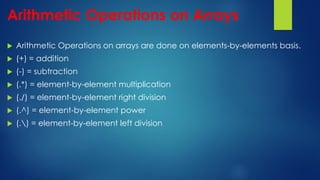
- 28. Arithmetic Operations on Arrays Arithmetic Operations on arrays are done on elements-by-elements basis. (+) = addition (-) = subtraction (.*) = element-by-element multiplication (./) = element-by-element right division (.^) = element-by-element power (.) = element-by-element left division
- 29. MATLAB Plotting Plotting is a graphical representation of a data set that shows a relationship between two or more variables. MATLAB plots play an essential role in the field of mathematics, science, engineering, technology and finance for statistics and data analysis. There are several functions available in MATLAB to create 2-D and 3-D plots.
- 30. 2-D Plots MATLAB plot() MATLAB fplot() MATLAB Semilogx() MATLAB Semilogy() MATLAB loglog() MATLAB polar() MATLAB fill() MATLAB bar() MATLAB barh() MATLAB plotyy() MATLAB area() MATLAB pie() MATLAB hist() MATLAB stem() MATLAB stairs()
- 31. 2-D MATLAB provides plotting capability with polar coordinates: polar(theta, r) Example r=2sin5t,0≤t≤2π
- 32. 3-D Plots MATLAB plot3() MATLAB pie3() MATLAB fill3() MATLAB contour3() MATLAB surf() MATLAB surfc() MATLAB mesh() MATLAB meshz() MATLAB waterfall() MATLAB stem3() MATLAB ribbon() MATLAB sphere() MATLAB ellipsoid() MATLAB cylinder() MATLAB slice()
- 33. 3-D MATLAB Surface surf(x,y,z) Example x = -5 to 5, y = -5 to 5, z = cos x cos y e (-√(x^2+y^2 ))/4
- 34. Linear Algebra A linear algebra equation is an equation of the system. Express the algebraic equations in matrix form, Ax = B. and find the value of x. 3x + 4y + z = 2 -2x + 3z = 1 1x +2y + 4z = 0 AX = B, X = B/A = inv(A)*B. X = AB
- 35. MATLAB Polynomial Polynomial Evaluation Roots of Polynomial Polynomial Addition Polynomial Subtraction Polynomial Multiplication Polynomial Division Polynomial Differentiation Polynomial Integration
- 36. Polynomial Functions MATLAB performs polynomial operations. P(x) = x4 + 7x3 - 5x + 9 Solution of this equation at 1, 9, 19 ,21 etc. P = [1 7 0 -5 9] x = 1 polycal(P,x)
- 37. Laplace Inverse Laplace Zeros, Poles , Pole-Zeros Map, State Space Representation Serial / Cascade, Parallel and Feedback Connections Step Response Impulse Response Root Locus Plots Bode Plots Nyquist Plots MATLAB Control System
- 38. Laplace Find the Laplace Transform of the function f(t) =e^-t(1-sin(t)) Solution The following command are used. syms t ft = exp(-t)*(1-sin(t)); fs = laplace(ft); The result of the commands is as follows fs = 1/(1+s)- 1/(2+2*s+s^2)
- 39. Inverse Laplace Find the Inverse Laplace Transform of the function F(s) = 1/(s+4) Solution The following command are used syms s t fs = 1/(s+4); ft = ilaplace(fs) The results of the command is ft = exp(-4*t) Inverse Laplace
- 40. MATLAB Applications in DSP Signal Processing Signals Classification Representation of Discrete Signals Signals Operation Addition Multiplication Scaling Folding Multi-rate Signal Processing Functions Fourier Transform Digital Filter Design IIR Digital Filter Design Filter Design and Analysis Tool
- 41. Signals Processing Signal Processing (a) Analog or Continuous Time Approach (b) Digital or Discrete Time Approach Discrete Signals Representation (a) Graphical Representation (b) Functional Representation (c) Tabular Representation (d) Sequential Representation
- 42. Graphical Representation A signal can be graphically represented using stem command in MATLAB. The syntax is given as: stem(x) stem(t,x) stem(t,x, ‘fill’) stem(t,x, ‘fill’, ‘----’ ) stem(t,x, ‘marker’)
- 43. Plot the sine wave in discrete signal form. 𝑡 = −𝜋 𝑡𝑜 𝜋, 𝑦 = sin(𝑡) Solution:- t = linspace(-pi, pi, 10); y = sin(t); stem(t, y) Using other command t = linspace(-pi, pi, 10); y = sin(t); stem(t, y, ‘fill’, ‘--’); title(‘plot of sine wave’); xlabel(‘discrete time’); ylabel(‘sine wave amplitude’);
- 44. Digital Filter Design The digital filters can be classified as: Finite-duration impulse response (FIR) filter Infinite-duration impulse response (IIR) filter IIR Digital Filter Design The different types of IIR digital filters are: Butterworth filter Chebyshev Type I filter Chebyshev Type II filter Elliptic filter
- 45. Filter Design and Analysis Tool The Different types of responses that can be viewed are listed below. Magnitude response Phase response Group delay Phase delay Impulse response Step response Pole-zero plot Zero-phase plot
- 46. MATLAB Simulink Simulink Modeling Wireless Communication Power Electronics Control Design Control Systems Signal Processing Robotics Advanced Driver Assistance Systems Image Processing and Computer Vision Etc.