Lecture5 kernel svm
1 like974 views

This document provides an overview of support vector machines (SVMs) as kernel machines. It discusses how SVMs can be formulated as optimization problems in reproducing kernel Hilbert spaces using kernels. Specifically, it covers: 1) How the SVM primal optimization problem can be solved using Lagrange multipliers and the representer theorem to obtain the dual quadratic program. 2) How the regularization parameter C in the C-SVM formulation allows data points to lie on or outside the margin. 3) The active set method for solving the SVM quadratic program, which iteratively optimizes over the sets of active and inactive constraints.


![Regularization path for SVM
min
f ∈H
n
i=1
max(1 − yi f (xi ), 0) +
λo
2
f 2
H
Iα is the set of support vectors s.t. yi f (xi ) = 1;
∂f J(f ) =
i∈Iα
γi yi K(xi , •) −
i∈I1
yi K(xi , •) + λo f (•) with γi ∈ ∂H(1) =] − 1, 0[](https://image.slidesharecdn.com/lecture5kernelsvm-140315083037-phpapp01/85/Lecture5-kernel-svm-25-320.jpg)
![Regularization path for SVM
min
f ∈H
n
i=1
max(1 − yi f (xi ), 0) +
λo
2
f 2
H
Iα is the set of support vectors s.t. yi f (xi ) = 1;
∂f J(f ) =
i∈Iα
γi yi K(xi , •) −
i∈I1
yi K(xi , •) + λo f (•) with γi ∈ ∂H(1) =] − 1, 0[
Let λn a value close enough to λo to keep the sets I0, Iα and IC unchanged
In particular at point xj ∈ Iα (fo(xj ) = fn(xj ) = yj ) : ∂f J(f )(xj ) = 0
i∈Iα
γioyi K(xi , xj ) = i∈I1
yi K(xi , xj ) − λo yj
i∈Iα
γinyi K(xi , xj ) = i∈I1
yi K(xi , xj ) − λn yj
G(γn − γo) = (λo − λn)y avec Gij = yi K(xi , xj )
γn = γo + (λo − λn)w
w = (G)−1
y](https://image.slidesharecdn.com/lecture5kernelsvm-140315083037-phpapp01/85/Lecture5-kernel-svm-26-320.jpg)
![Example of regularization path
γi ∈] − 1, 0[ yi γi ∈] − 1, −1[ λ =
1
C
γi = − 1
C αi ; performing together estimation and data selection](https://image.slidesharecdn.com/lecture5kernelsvm-140315083037-phpapp01/85/Lecture5-kernel-svm-27-320.jpg)
![How to choose and P to get linear regularization path?
the path is piecewise linear ⇔
one is piecewise quadratic
and the other is piecewise linear
the convex case [Rosset & Zhu, 07]
min
β∈IRd
(β) + λP(β)
1 piecewise linearity: lim
ε→0
β(λ + ε) − β(λ)
ε
= constant
2 optimality
(β(λ)) + λ P(β(λ)) = 0
(β(λ + ε)) + (λ + ε) P(β(λ + ε)) = 0
3 Taylor expension
lim
ε→0
β(λ + ε) − β(λ)
ε
= 2
(β(λ)) + λ 2
P(β(λ))
−1
P(β(λ))
2
(β(λ)) = constant and 2
P(β(λ)) = 0](https://image.slidesharecdn.com/lecture5kernelsvm-140315083037-phpapp01/85/Lecture5-kernel-svm-28-320.jpg)

![ν-SVM and other formulations...
ν ∈ [0, 1]
(ν)
min
f ,b,ξ,m
1
2 f 2
H + 1
np
n
i=1
ξp
i − νm
with yi f (xi ) + b ≥ m − ξi , i = 1, n,
and m ≥ 0, ξi ≥ 0, i = 1, n,
for p = 1 the dual formulation is:
max
α∈IRn
−1
2 α Gα
with α y = 0 et 0 ≤ αi ≤ 1
n i = 1, n
and ν ≤ α 1I
C = 1
m](https://image.slidesharecdn.com/lecture5kernelsvm-140315083037-phpapp01/85/Lecture5-kernel-svm-31-320.jpg)


Lecture5 kernel svm
- 1. Lecture 5: SVM as a kernel machine Stéphane Canu stephane.canu@litislab.eu Sao Paulo 2014 March 4, 2014
- 2. Plan 1 Kernel machines Non sparse kernel machines sparse kernel machines: SVM SVM: variations on a theme Sparse kernel machines for regression: SVR
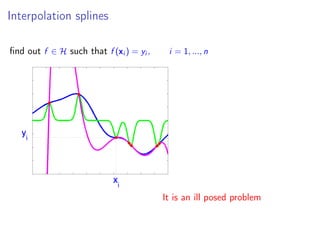
- 3. Interpolation splines find out f ∈ H such that f (xi ) = yi , i = 1, ..., n It is an ill posed problem
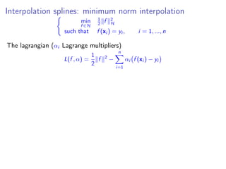
- 4. Interpolation splines: minimum norm interpolation min f ∈H 1 2 f 2 H such that f (xi ) = yi , i = 1, ..., n The lagrangian (αi Lagrange multipliers) L(f , α) = 1 2 f 2 − n i=1 αi f (xi ) − yi
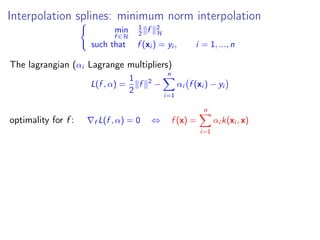
- 5. Interpolation splines: minimum norm interpolation min f ∈H 1 2 f 2 H such that f (xi ) = yi , i = 1, ..., n The lagrangian (αi Lagrange multipliers) L(f , α) = 1 2 f 2 − n i=1 αi f (xi ) − yi optimality for f : f L(f , α) = 0 ⇔ f (x) = n i=1 αi k(xi , x)
- 6. Interpolation splines: minimum norm interpolation min f ∈H 1 2 f 2 H such that f (xi ) = yi , i = 1, ..., n The lagrangian (αi Lagrange multipliers) L(f , α) = 1 2 f 2 − n i=1 αi f (xi ) − yi optimality for f : f L(f , α) = 0 ⇔ f (x) = n i=1 αi k(xi , x) dual formulation (remove f from the lagrangian): Q(α) = − 1 2 n i=1 n j=1 αi αj k(xi , xj ) + n i=1 αi yi solution: max α∈IRn Q(α) Kα = y
- 7. Representer theorem Theorem (Representer theorem) Let H be a RKHS with kernel k(s, t). Let be a function from X to IR (loss function) and Φ a non decreasing function from IR to IR. If there exists a function f ∗minimizing: f ∗ = argmin f ∈H n i=1 yi , f (xi ) + Φ f 2 H then there exists a vector α ∈ IRn such that: f ∗ (x) = n i=1 αi k(x, xi ) it can be generalized to the semi parametric case: + m j=1 βj φj (x)
- 8. Elements of a proof 1 Hs = span{k(., x1), ..., k(., xi ), ..., k(., xn)} 2 orthogonal decomposition: H = Hs ⊕ H⊥ ⇒ ∀f ∈ H; f = fs + f⊥ 3 pointwise evaluation decomposition f (xi ) = fs(xi ) + f⊥(xi ) = fs(.), k(., xi ) H + f⊥(.), k(., xi ) H =0 = fs(xi ) 4 norm decomposition f 2 H = fs 2 H + f⊥ 2 H ≥0 ≥ fs 2 H 5 decompose the global cost n i=1 yi , f (xi ) + Φ f 2 H = n i=1 yi , fs(xi ) + Φ fs 2 H + f⊥ 2 H ≥ n i=1 yi , fs(xi ) + Φ fs 2 H 6 argmin f ∈H = argmin f ∈Hs .
- 9. Smooting splines introducing the error (the slack) ξ = f (xi ) − yi (S) min f ∈H 1 2 f 2 H + 1 2λ n i=1 ξ2 i such that f (xi ) = yi + ξi , i = 1, n three equivalent definitions (S ) min f ∈H 1 2 n i=1 f (xi ) − yi 2 + λ 2 f 2 H min f ∈H 1 2 f 2 H such that n i=1 f (xi ) − yi 2 ≤ C min f ∈H n i=1 f (xi ) − yi 2 such that f 2 H ≤ C using the representer theorem (S ) min α∈IRn 1 2 Kα − y 2 + λ 2 α Kα solution: (S) ⇔ (S ) ⇔ (S ) ⇔ (K + λI)α = y = ridge regression: min α∈IRn 1 2 Kα − y 2 + λ 2 α α
- 10. Kernel logistic regression inspiration: the Bayes rule D(x) = sign f (x) + α0 =⇒ log IP(Y =1|x) IP(Y =−1|x) = f (x) + α0 probabilities: IP(Y = 1|x) = expf (x)+α0 1 + expf (x)+α0 IP(Y = −1|x) = 1 1 + expf (x)+α0 Rademacher distribution L(xi , yi , f , α0) = IP(Y = 1|xi ) yi +1 2 (1 − IP(Y = 1|xi )) 1−yi 2 penalized likelihood J(f , α0) = − n i=1 log L(xi , yi , f , α0) + λ 2 f 2 H = n i=1 log 1 + exp−yi (f (xi )+α0) + λ 2 f 2 H
- 11. Kernel logistic regression (2) (R) min f ∈H 1 2 f 2 H + 1 λ n i=1 log 1 + exp−ξi with ξi = yi (f (xi ) + α0) , i = 1, n Representer theorem J(α, α0) = 1I log 1I + expdiag(y)Kα+α0y + λ 2 α Kα gradient vector anf Hessian matrix: αJ(α, α0) = K y − (2p − 1I) + λKα HαJ(α, α0) = Kdiag p(1I − p) K + λK solve the problem using Newton iterations αnew = αold + Kdiag p(1I − p) K + λK −1 K y − (2p − 1I) + λα
- 12. Let’s summarize pros Universality from H to IRn using the representer theorem no (explicit) curse of dimensionality splines O(n3) (can be reduced to O(n2)) logistic regression O(kn3) (can be reduced to O(kn2) no scalability! sparsity comes to the rescue!
- 13. Roadmap 1 Kernel machines Non sparse kernel machines sparse kernel machines: SVM SVM: variations on a theme Sparse kernel machines for regression: SVR Stéphane Canu (INSA Rouen - LITIS) March 4, 2014 11 / 38
- 14. SVM in a RKHS: the separable case (no noise) max f ,b m with yi f (xi ) + b ≥ m and f 2 H = 1 ⇔ min f ,b 1 2 f 2 H with yi f (xi ) + b ≥ 1 3 ways to represent function f f (x) in the RKHS H = d j=1 wj φj (x) d features = n i=1 αi yi k(x, xi ) n data points min w,b 1 2 w 2 IRd = 1 2 w w with yi w φ(xi ) + b ≥ 1 ⇔ min α,b 1 2 α Kα with yi α K(:, i) + b ≥ 1
- 15. using relevant features... a data point becomes a function x −→ k(x, •)
- 16. Representer theorem for SVM min f ,b 1 2 f 2 H with yi f (xi ) + b ≥ 1 Lagrangian L(f , b, α) = 1 2 f 2 H − n i=1 αi yi (f (xi ) + b) − 1 α ≥ 0 optimility condition: f L(f , b, α) = 0 ⇔ f (x) = n i=1 αi yi k(xi , x) Eliminate f from L: f 2 H = n i=1 n j=1 αi αj yi yj k(xi , xj ) n i=1 αi yi f (xi ) = n i=1 n j=1 αi αj yi yj k(xi , xj ) Q(b, α) = − 1 2 n i=1 n j=1 αi αj yi yj k(xi , xj ) − n i=1 αi yi b − 1
- 17. Dual formulation for SVM the intermediate function Q(b, α) = − 1 2 n i=1 n j=1 αi αj yi yj k(xi , xj ) − b n i=1 αi yi + n i=1 αi max α min b Q(b, α) b can be seen as the Lagrange multiplier of the following (balanced) constaint n i=1 αi yi = 0 which is also the optimality KKT condition on b Dual formulation max α∈IRn −1 2 n i=1 n j=1 αi αj yi yj k(xi , xj ) + n i=1 αi such that n i=1 αi yi = 0 and 0 ≤ αi , i = 1, n
- 18. SVM dual formulation Dual formulation max α∈IRn −1 2 n i=1 n j=1 αi αj yi yj k(xi , xj ) + n i=1 αi with n i=1 αi yi = 0 and 0 ≤ αi , i = 1, n The dual formulation gives a quadratic program (QP) min α∈IRn 1 2 α Gα − I1 α with α y = 0 and 0 ≤ α with Gij = yi yj k(xi , xj ) with the linear kernel f (x) = n i=1 αi yi (x xi ) = d j=1 βj xj when d is small wrt. n primal may be interesting.
- 19. the general case: C-SVM Primal formulation (P) min f ∈H,b,ξ∈IRn 1 2 f 2 + C p n i=1 ξp i such that yi f (xi ) + b ≥ 1 − ξi , ξi ≥ 0, i = 1, n C is the regularization path parameter (to be tuned) p = 1 , L1 SVM max α∈IRn −1 2 α Gα + α 1I such that α y = 0 and 0 ≤ αi ≤ C i = 1, n p = 2, L2 SVM max α∈IRn −1 2 α G + 1 C I α + α 1I such that α y = 0 and 0 ≤ αi i = 1, n the regularization path: is the set of solutions α(C) when C varies
- 20. Data groups: illustration f (x) = n i=1 αi k(x, xi ) D(x) = sign f (x) + b useless data important data suspicious data well classified support α = 0 0 < α < C α = C the regularization path: is the set of solutions α(C) when C varies
- 21. The importance of being support f (x) = n i=1 αi yi k(xi , x) data point α constraint value set xi useless αi = 0 yi f (xi ) + b > 1 I0 xi support 0 < αi < C yi f (xi ) + b = 1 Iα xi suspicious αi = C yi f (xi ) + b < 1 IC Table: When a data point is « support » it lies exactly on the margin. here lies the efficiency of the algorithm (and its complexity)! sparsity: αi = 0
- 22. The active set method for SVM (1) min α∈IRn 1 2 α Gα − α 1I such that α y = 0 i = 1, n and 0 ≤ αi i = 1, n Gα − 1I − β + by = 0 α y = 0 0 ≤ αi i = 1, n 0 ≤ βi i = 1, n αi βi = 0 i = 1, n αa 0 − − + b 1 1 0 β0 ya y0 = 0 0 G α − −1I β + b y = 0 Ga Gi G0 Gi (1) Gaαa − 1Ia + bya = 0 (2) Gi αa − 1I0 − β0 + by0 = 0 1 solve (1) (find α together with b) 2 if α < 0 move it from Iα to I0 goto 1 3 else solve (2) if β < 0 move it from I0 to Iα goto 1
- 23. The active set method for SVM (2) Function (α, b, Iα) ←Solve_QP_Active_Set(G, y) % Solve minα 1/2α Gα − 1I α % s.t. 0 ≤ α and y α = 0 (Iα, I0, α) ← initialization while The_optimal_is_not_reached do (α, b) ← solve Gaαa − 1Ia + bya ya αa = 0 if ∃i ∈ Iα such that αi < 0 then α ← projection( αa, α) move i from Iα to I0 else if ∃j ∈ I0 such that βj < 0 then use β0 = y0(Ki αa + b1I0) − 1I0 move j from I0 to Iα else The_optimal_is_not_reached ← FALSE end if end while α αold αnew Projection step of the active constraints algorithm d = alpha - alphaold; alpha = alpha + t * d; Caching Strategy Save space and computing time by computing only the needed parts of kernel matrix G
- 24. Two more ways to derivate SVM Using the hinge loss min f ∈H,b∈IR 1 p n i=1 max 0, 1 − yi (f (xi ) + b) p + 1 2C f 2 Minimizing the distance between the convex hulls min α u − v 2 H with u(x) = {i|yi =1} αi k(xi , x), v(x) = {i|yi =−1} αi k(xi , x) and {i|yi =1} αi = 1, {i|yi =−1} αi = 1, 0 ≤ αi i = 1, n f (x) = 2 u − v 2 H u(x) − v(x) and b = u 2 H − v 2 H u − v 2 H the regularization path: is the set of solutions α(C) when C varies
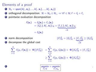
- 25. Regularization path for SVM min f ∈H n i=1 max(1 − yi f (xi ), 0) + λo 2 f 2 H Iα is the set of support vectors s.t. yi f (xi ) = 1; ∂f J(f ) = i∈Iα γi yi K(xi , •) − i∈I1 yi K(xi , •) + λo f (•) with γi ∈ ∂H(1) =] − 1, 0[
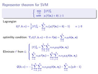
- 26. Regularization path for SVM min f ∈H n i=1 max(1 − yi f (xi ), 0) + λo 2 f 2 H Iα is the set of support vectors s.t. yi f (xi ) = 1; ∂f J(f ) = i∈Iα γi yi K(xi , •) − i∈I1 yi K(xi , •) + λo f (•) with γi ∈ ∂H(1) =] − 1, 0[ Let λn a value close enough to λo to keep the sets I0, Iα and IC unchanged In particular at point xj ∈ Iα (fo(xj ) = fn(xj ) = yj ) : ∂f J(f )(xj ) = 0 i∈Iα γioyi K(xi , xj ) = i∈I1 yi K(xi , xj ) − λo yj i∈Iα γinyi K(xi , xj ) = i∈I1 yi K(xi , xj ) − λn yj G(γn − γo) = (λo − λn)y avec Gij = yi K(xi , xj ) γn = γo + (λo − λn)w w = (G)−1 y
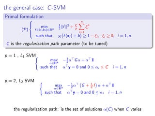
- 27. Example of regularization path γi ∈] − 1, 0[ yi γi ∈] − 1, −1[ λ = 1 C γi = − 1 C αi ; performing together estimation and data selection
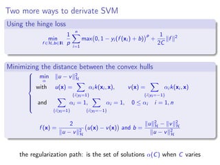
- 28. How to choose and P to get linear regularization path? the path is piecewise linear ⇔ one is piecewise quadratic and the other is piecewise linear the convex case [Rosset & Zhu, 07] min β∈IRd (β) + λP(β) 1 piecewise linearity: lim ε→0 β(λ + ε) − β(λ) ε = constant 2 optimality (β(λ)) + λ P(β(λ)) = 0 (β(λ + ε)) + (λ + ε) P(β(λ + ε)) = 0 3 Taylor expension lim ε→0 β(λ + ε) − β(λ) ε = 2 (β(λ)) + λ 2 P(β(λ)) −1 P(β(λ)) 2 (β(λ)) = constant and 2 P(β(λ)) = 0
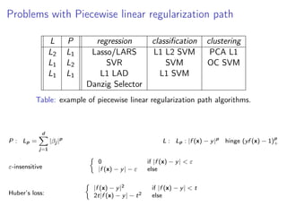
- 29. Problems with Piecewise linear regularization path L P regression classification clustering L2 L1 Lasso/LARS L1 L2 SVM PCA L1 L1 L2 SVR SVM OC SVM L1 L1 L1 LAD L1 SVM Danzig Selector Table: example of piecewise linear regularization path algorithms. P : Lp = d j=1 |βj |p L : Lp : |f (x) − y|p hinge (yf (x) − 1)p + ε-insensitive 0 if |f (x) − y| < ε |f (x) − y| − ε else Huber’s loss: |f (x) − y|2 if |f (x) − y| < t 2t|f (x) − y| − t2 else
- 30. SVM with non symmetric costs problem in the primal min f ∈H,b,ξ∈IRn 1 2 f 2 H + C+ {i|yi =1} ξp i + C− {i|yi =−1} ξp i with yi f (xi ) + b ≥ 1 − ξi , ξi ≥ 0, i = 1, n for p = 1 the dual formulation is the following: max α∈IRn −1 2 α Gα + α 1I with α y = 0 and 0 ≤ αi ≤ C+ or C− i = 1, n
- 31. ν-SVM and other formulations... ν ∈ [0, 1] (ν) min f ,b,ξ,m 1 2 f 2 H + 1 np n i=1 ξp i − νm with yi f (xi ) + b ≥ m − ξi , i = 1, n, and m ≥ 0, ξi ≥ 0, i = 1, n, for p = 1 the dual formulation is: max α∈IRn −1 2 α Gα with α y = 0 et 0 ≤ αi ≤ 1 n i = 1, n and ν ≤ α 1I C = 1 m
- 32. Generalized SVM min f ∈H,b∈IR n i=1 max 0, 1 − yi (f (xi ) + b) + 1 C ϕ(f ) ϕ convex in particular ϕ(f ) = f p p with p = 1 leads to L1 SVM. min α∈IRn,b,ξ 1I β + C1I ξ with yi n j=1 αj k(xi , xj ) + b ≥ 1 − ξi , and −βi ≤ αi ≤ βi , ξi ≥ 0, i = 1, n with β = |α|. the dual is: max γ,δ,δ∗∈IR3n 1I γ with y γ = 0, δi + δ∗ i = 1 n j=1 γj k(xi , xj ) = δi − δ∗ i , i = 1, n and 0 ≤ δi , 0 ≤ δ∗ i , 0 ≤ γi ≤ C, i = 1, n Mangassarian, 2001
- 33. K-Lasso (Kernel Basis pursuit) The Kernel Lasso (S1) min α∈IRn 1 2 Kα − y 2 + λ n i=1 |αi | Typical parametric quadratic program (pQP) with αi = 0 Piecewise linear regularization path The dual: (D1) min α 1 2 Kα 2 such that K (Kα − y) ≤ t The K-Danzig selector can be treated the same way require to compute K K - no more function f !
- 34. Support vector regression (SVR) Lasso’s dual adaptation: min α 1 2 Kα 2 s. t. K (Kα − y) ≤ t min f ∈H 1 2 f 2 H s. t. |f (xi ) − yi | ≤ t, i = 1, n The support vector regression introduce slack variables (SVR) min f ∈H 1 2 f 2 H + C |ξi | such that |f (xi ) − yi | ≤ t + ξi 0 ≤ ξi i = 1, n a typical multi parametric quadratic program (mpQP) piecewise linear regularization path α(C, t) = α(C0, t0) + ( 1 C − 1 C0 )u + 1 C0 (t − t0)v 2d Pareto’s front (the tube width and the regularity)
- 35. Support vector regression illustration 0 1 2 3 4 5 6 7 8 −1 −0.8 −0.6 −0.4 −0.2 0 0.2 0.4 0.6 0.8 1 Support Vector Machine Regression x y 0 0.5 1 1.5 2 2.5 3 3.5 4 4.5 5 −1.5 −1 −0.5 0 0.5 1 1.5 Support Vector Machine Regression x y C large C small there exists other formulations such as LP SVR...
- 36. SVM reduction (reduced set method)) objective: compile the model f (x) = ns i=1 αi k(xi , x), ns n, ns too big compiled model as the solution of: g(x) = nc i=1 βi k(zi , x), nc ns β, zi and c are tuned by minimizing: min β,zi g − f 2 H where min β,zi g − f 2 H = α Kx α + β Kz β − 2α Kxz β some authors advice 0, 03 ≤ nc ns ≤ 0, 1 solve it by using use (stochastic) gradient (its a RBF problem) Burges 1996, Ozuna 1997, Romdhani 2001
- 37. logistic regression and the import vector machine Logistic regression is NON sparse kernalize it using the dictionary strategy Algorithm: find the solution of the KLR using only a subset S of the data build S iteratively using active constraint approach this trick brings sparsity it estimates probability it can naturally be generalized to the multiclass case efficent when uses: a few import vectors component-wise update procedure extention using L1 KLR Zhu & Hastie, 01 ; Keerthi et. al., 02
- 38. Historical perspective on kernel machines statistics 1960 Parzen, Nadaraya Watson 1970 Splines 1980 Kernels: Silverman, Hardle... 1990 sparsity: Donoho (pursuit), Tibshirani (Lasso)... Statistical learning 1985 Neural networks: non linear - universal structural complexity non convex optimization 1992 Vapnik et. al. theory - regularization - consistancy convexity - Linearity Kernel - universality sparsity results: MNIST Stéphane Canu (INSA Rouen - LITIS) March 4, 2014 35 / 38
- 39. what’s new since 1995 Applications kernlisation w x → f , k(x, .) H kernel engineering sturtured outputs applications: image, text, signal, bio-info... Optimization dual: mloss.org regularization path approximation primal Statistic proofs and bounds model selection span bound multikernel: tuning (k and σ) Stéphane Canu (INSA Rouen - LITIS) March 4, 2014 36 / 38
- 40. challenges: towards tough learning the size effect ready to use: automatization adaptative: on line context aware beyond kenrels Automatic and adaptive model selection variable selection kernel tuning (k et σ) hyperparametres: C, duality gap, λ IP change Theory non positive kernels a more general representer theorem Stéphane Canu (INSA Rouen - LITIS) March 4, 2014 37 / 38
- 41. biblio: kernel-machines.org John Shawe-Taylor and Nello Cristianini Kernel Methods for Pattern Analysis, Cambridge University Press, 2004 Bernhard Schölkopf and Alex Smola. Learning with Kernels. MIT Press, Cambridge, MA, 2002. Trevor Hastie, Robert Tibshirani and Jerome Friedman, The Elements of Statistical Learning:. Data Mining, Inference, and Prediction, springer, 2001 Léon Bottou, Olivier Chapelle, Dennis DeCoste and Jason Weston Large-Scale Kernel Machines (Neural Information Processing, MIT press 2007 Olivier Chapelle, Bernhard Scholkopf and Alexander Zien, Semi-supervised Learning, MIT press 2006 Vladimir Vapnik. Estimation of Dependences Based on Empirical Data. Springer Verlag, 2006, 2nd edition. Vladimir Vapnik. The Nature of Statistical Learning Theory. Springer, 1995. Grace Wahba. Spline Models for Observational Data. SIAM CBMS-NSF Regional Conference Series in Applied Mathematics vol. 59, Philadelphia, 1990 Alain Berlinet and Christine Thomas-Agnan, Reproducing Kernel Hilbert Spaces in Probability and Statistics,Kluwer Academic Publishers, 2003 Marc Atteia et Jean Gaches , Approximation Hilbertienne - Splines, Ondelettes, Fractales, PUG, 1999 Stéphane Canu (INSA Rouen - LITIS) March 4, 2014 38 / 38