SlideShare a Scribd company logo
Section 4.5
                     Optimization II

                     V63.0121.021, Calculus I

                          New York University


                         class supplement


Announcements

   Quiz 5 on §§4.1–4.4 next week in recitation
   Happy Thanksgiving!

                                                .   .   .   .   .   .
Announcements


         Quiz 5 on §§4.1–4.4 next
         week in recitation
         Happy Thanksgiving!


                                                                .   .   .        .      .      .

 V63.0121.021, Calculus I (NYU)   Section 4.5 Optimization II               class supplement       2 / 25
Objectives


         Given a problem requiring
         optimization, identify the
         objective functions,
         variables, and constraints.
         Solve optimization
         problems with calculus.


                                                                .   .   .        .      .      .

 V63.0121.021, Calculus I (NYU)   Section 4.5 Optimization II               class supplement       3 / 25
Outline


Recall


More examples
  Addition
  Distance
  Triangles
  Economics
  The Statue of Liberty


                                                                .   .   .        .      .      .

 V63.0121.021, Calculus I (NYU)   Section 4.5 Optimization II               class supplement       4 / 25
Checklist for optimization problems


 1. Understand the Problem What is known? What is unknown?
    What are the conditions?
 2. Draw a diagram
 3. Introduce Notation
 4. Express the “objective function” Q in terms of the other symbols
 5. If Q is a function of more than one “decision variable”, use the
    given information to eliminate all but one of them.
 6. Find the absolute maximum (or minimum, depending on the
    problem) of the function on its domain.


                                                                .   .   .        .      .      .

 V63.0121.021, Calculus I (NYU)   Section 4.5 Optimization II               class supplement       5 / 25
Recall: The Closed Interval Method
See Section 4.1


The Closed Interval Method
To find the extreme values of a function f on [a, b], we need to:
       Evaluate f at the endpoints a and b
       Evaluate f at the critical points x where either f′ (x) = 0 or f is not
       differentiable at x.
       The points with the largest function value are the global maximum
       points
       The points with the smallest/most negative function value are the
       global minimum points.


                                                                 .   .   .        .      .      .

  V63.0121.021, Calculus I (NYU)   Section 4.5 Optimization II               class supplement       6 / 25
Recall: The First Derivative Test
See Section 4.3

Theorem (The First Derivative Test)
Let f be continuous on (a, b) and c a critical point of f in (a, b).
       If f′ changes from negative to positive at c, then c is a local
       minimum.
       If f′ changes from positive to negative at c, then c is a local
       maximum.
       If f′ does not change sign at c, then c is not a local extremum.


                                                                 .   .   .        .      .      .

  V63.0121.021, Calculus I (NYU)   Section 4.5 Optimization II               class supplement       7 / 25
Recall: The First Derivative Test
See Section 4.3

Theorem (The First Derivative Test)
Let f be continuous on (a, b) and c a critical point of f in (a, b).
       If f′ changes from negative to positive at c, then c is a local
       minimum.
       If f′ changes from positive to negative at c, then c is a local
       maximum.
       If f′ does not change sign at c, then c is not a local extremum.

Corollary

       If f′ < 0 for all x < c and f′ (x) > 0 for all x > c, then c is the global
       minimum of f on (a, b).
       If f′ < 0 for all x > c and f′ (x) > 0 for all x < c, then c is the global
       maximum of f on (a, b).
                                                                 .   .   .        .      .      .

  V63.0121.021, Calculus I (NYU)   Section 4.5 Optimization II               class supplement       7 / 25
Recall: The Second Derivative Test
See Section 4.3

Theorem (The Second Derivative Test)
Let f, f′ , and f′′ be continuous on [a, b]. Let c be in (a, b) with f′ (c) = 0.
       If f′′ (c) < 0, then f(c) is a local maximum.
       If f′′ (c) > 0, then f(c) is a local minimum.


                                                                 .   .   .        .      .      .

  V63.0121.021, Calculus I (NYU)   Section 4.5 Optimization II               class supplement       8 / 25
Recall: The Second Derivative Test
See Section 4.3

Theorem (The Second Derivative Test)
Let f, f′ , and f′′ be continuous on [a, b]. Let c be in (a, b) with f′ (c) = 0.
       If f′′ (c) < 0, then f(c) is a local maximum.
       If f′′ (c) > 0, then f(c) is a local minimum.

Warning
If f′′ (c) = 0, the second derivative test is inconclusive (this does not
mean c is neither; we just don’t know yet).

Corollary

       If f′ (c) = 0 and f′′ (x) > 0 for all x, then c is the global minimum of f
       If f′ (c) = 0 and f′′ (x) < 0 for all x, then c is the global maximum of f
                                                                 .   .   .        .      .      .

  V63.0121.021, Calculus I (NYU)   Section 4.5 Optimization II               class supplement       8 / 25
Which to use when?

            CIM                     1DT                             2DT
 Pro        – no need for           – works on                      – works on
            inequalities            non-closed,                     non-closed,
            – gets global           non-bounded                     non-bounded
            extrema                 intervals                       intervals
            automatically           – only one derivative           – no need for
                                                                    inequalities
 Con        – only for closed       – Uses inequalities             – More derivatives
            bounded intervals       – More work at                  – less conclusive
                                    boundary than CIM               than 1DT
                                                                    – more work at
                                                                    boundary than CIM


                                                                .   .   .        .      .      .

 V63.0121.021, Calculus I (NYU)   Section 4.5 Optimization II               class supplement       9 / 25
Which to use when?

            CIM                     1DT                             2DT
 Pro        – no need for           – works on                      – works on
            inequalities            non-closed,                     non-closed,
            – gets global           non-bounded                     non-bounded
            extrema                 intervals                       intervals
            automatically           – only one derivative           – no need for
                                                                    inequalities
 Con        – only for closed       – Uses inequalities             – More derivatives
            bounded intervals       – More work at                  – less conclusive
                                    boundary than CIM               than 1DT
                                                                    – more work at
                                                                    boundary than CIM

      Use CIM if it applies: the domain is a closed, bounded interval
      If domain is not closed or not bounded, use 2DT if you like to take
      derivatives, or 1DT if you like to compare signs.
                                                                .   .   .        .      .      .

 V63.0121.021, Calculus I (NYU)   Section 4.5 Optimization II               class supplement       9 / 25
Outline


Recall


More examples
  Addition
  Distance
  Triangles
  Economics
  The Statue of Liberty


                                                                .   .   .         .       .    .

 V63.0121.021, Calculus I (NYU)   Section 4.5 Optimization II               class supplement   10 / 25
Addition with a constraint
Example
Find two positive numbers x and y with xy = 16 and x + y as small as
possible.


                                                                .   .   .         .      .     .

 V63.0121.021, Calculus I (NYU)   Section 4.5 Optimization II               class supplement   11 / 25
Addition with a constraint
Example
Find two positive numbers x and y with xy = 16 and x + y as small as
possible.

Solution

      Objective: minimize S = x + y subject to the constraint that
      xy = 16
      Eliminate y: y = 16/x so S = x + 16/x. The domain of
      consideration is (0, ∞).
      Find the critical points: S′ (x) = 1 − 16/x2 , which is 0 when x = 4.
      Classify the critical points: S′′ (x) = 32/x3 , which is always
      positive. So the graph is always concave up, 4 is a local min, and
      therefore the global min.
      So the numbers are x = y = 4, Smin = 8.
                                                                .   .   .         .      .     .

 V63.0121.021, Calculus I (NYU)   Section 4.5 Optimization II               class supplement   11 / 25
Distance
Example
Find the point P on the parabola y = x2 closest to the point (3, 0).


                                                                .   .   .         .       .    .

 V63.0121.021, Calculus I (NYU)   Section 4.5 Optimization II               class supplement   12 / 25
Distance
Example
Find the point P on the parabola y = x2 closest to the point (3, 0).


Solution
                                                                y


                                                                (x, x2 )

                                                                 .                                        x
                                                                     .     .   .         .   3   .    .

 V63.0121.021, Calculus I (NYU)   Section 4.5 Optimization II                      class supplement   12 / 25
Distance
Example
Find the point P on the parabola y = x2 closest to the point (3, 0).


Solution
                                                                y
The distance between (x, x2 )
and (3, 0) is given by
         √
 f(x) = (x − 3)2 + (x2 − 0)2

 We may instead minimize the
square of f:

  g(x) = f(x)2 = (x − 3)2 + x4                                  (x, x2 )

                                                                 .                                        x
The domain is (−∞, ∞).
                                                                     .     .   .         .   3   .    .

 V63.0121.021, Calculus I (NYU)   Section 4.5 Optimization II                      class supplement   12 / 25
Distance problem
minimization step


 We want to find the global minimum of g(x) = (x − 3)2 + x4 .


                                                                 .   .   .         .       .    .

  V63.0121.021, Calculus I (NYU)   Section 4.5 Optimization II               class supplement   13 / 25
Distance problem
minimization step


 We want to find the global minimum of g(x) = (x − 3)2 + x4 .
       g′ (x) = 2(x − 3) + 4x3 = 4x3 + 2x − 6 = 2(2x3 + x − 3)
       If a polynomial has integer roots, they are factors of the constant
       term (Euler)
       1 is a root, so 2x3 + x − 3 is divisible by x − 1:

                       f′ (x) = 2(2x3 + x − 3) = 2(x − 1)(2x2 + 2x + 3)

       The quadratic has no real roots (the discriminant b2 − 4ac < 0)


                                                                   .   .   .         .       .    .

  V63.0121.021, Calculus I (NYU)     Section 4.5 Optimization II               class supplement   13 / 25
Distance problem
minimization step


 We want to find the global minimum of g(x) = (x − 3)2 + x4 .
       g′ (x) = 2(x − 3) + 4x3 = 4x3 + 2x − 6 = 2(2x3 + x − 3)
       If a polynomial has integer roots, they are factors of the constant
       term (Euler)
       1 is a root, so 2x3 + x − 3 is divisible by x − 1:

                       f′ (x) = 2(2x3 + x − 3) = 2(x − 1)(2x2 + 2x + 3)

       The quadratic has no real roots (the discriminant b2 − 4ac < 0)
       We see f′ (1) = 0, f′ (x) < 0 if x < 1, and f′ (x) > 0 if x > 1. So 1 is
       the global minimum.
       The point on the parabola closest to (3, 0) is (1, 1). The minimum
                  √
       distance is 5.
                                                                   .   .   .         .       .    .

  V63.0121.021, Calculus I (NYU)     Section 4.5 Optimization II               class supplement   13 / 25
Remark


      We’ve used each of the methods (CIM, 1DT, 2DT) so far.
      Notice how we argued that the critical points were absolute
      extremes even though 1DT and 2DT only tell you relative/local
      extremes.


                                                                .   .   .         .       .    .

 V63.0121.021, Calculus I (NYU)   Section 4.5 Optimization II               class supplement   14 / 25
A problem with a triangle
.
Example
Find the rectangle of maximal area inscribed in a 3-4-5 right triangle with two
sides on legs of the triangle and one vertex on the hypotenuse.

Solution


                                                                           5
                                                                                         4


                                                                   .
                                                                           3

                                                                       .   .   .         .       .    .

    V63.0121.021, Calculus I (NYU)   Section 4.5 Optimization II                   class supplement   15 / 25
A problem with a triangle
.
Example
Find the rectangle of maximal area inscribed in a 3-4-5 right triangle with two
sides on legs of the triangle and one vertex on the hypotenuse.

Solution
         Let the dimensions of the
         rectangle be x and y.


                                                                               5   x
                                                                                             4

                                                                           y

                                                                   .
                                                                               3

                                                                       .       .   .         .       .    .

    V63.0121.021, Calculus I (NYU)   Section 4.5 Optimization II                       class supplement   15 / 25
A problem with a triangle
.
Example
Find the rectangle of maximal area inscribed in a 3-4-5 right triangle with two
sides on legs of the triangle and one vertex on the hypotenuse.

Solution
         Let the dimensions of the
         rectangle be x and y.
         Similar triangles give

           y    4
              =   =⇒ 3y = 4(3 − x)
          3−x   3                                                              5   x
                                                                                             4
                   4
         So y = 4 − x and                                                  y
                   3
                 (      )
                      4       4                                    .
         A(x) = x 4 − x = 4x − x2
                      3       3                                                3

                                                                       .       .   .         .       .    .

    V63.0121.021, Calculus I (NYU)   Section 4.5 Optimization II                       class supplement   15 / 25
Triangle Problem
maximization step


                                                    4
 We want to find the absolute maximum of A(x) = 4x − x2 on the
                                                    3
 interval [0, 3].


                                                                .   .   .         .       .    .

 V63.0121.021, Calculus I (NYU)   Section 4.5 Optimization II               class supplement   16 / 25
Triangle Problem
maximization step


                                                    4
 We want to find the absolute maximum of A(x) = 4x − x2 on the
                                                    3
 interval [0, 3].
      A(0) = A(3) = 0
                  8                          12
      A′ (x) = 4 − x, which is zero when x =    = 1.5.
                  3                          8


                                                                .   .   .         .       .    .

 V63.0121.021, Calculus I (NYU)   Section 4.5 Optimization II               class supplement   16 / 25
Triangle Problem
maximization step


                                                    4
 We want to find the absolute maximum of A(x) = 4x − x2 on the
                                                    3
 interval [0, 3].
      A(0) = A(3) = 0
                  8                            12
      A′ (x) = 4 − x, which is zero when x =      = 1.5.
                  3                            8
      Since A(1.5) = 3, this is the absolute maximum.
      So the dimensions of the rectangle of maximal area are 1.5 × 2.


                                                                .   .   .         .       .    .

 V63.0121.021, Calculus I (NYU)   Section 4.5 Optimization II               class supplement   16 / 25
An Economics problem
Example
Let r be the monthly rent per unit in an apartment building with 100
units. A survey reveals that all units can be rented when r = 900 and
that one unit becomes vacant with each 10 increase in rent. Suppose
the average monthly maintenance costs per occupied unit is
$100/month. What rent should be charged to maximize profit?


                                                                .   .   .         .       .    .

 V63.0121.021, Calculus I (NYU)   Section 4.5 Optimization II               class supplement   17 / 25
An Economics problem
Example
Let r be the monthly rent per unit in an apartment building with 100
units. A survey reveals that all units can be rented when r = 900 and
that one unit becomes vacant with each 10 increase in rent. Suppose
the average monthly maintenance costs per occupied unit is
$100/month. What rent should be charged to maximize profit?

Solution

      Let n be the number of units rented, depending on price (the
      demand function).
                                  ∆n        1
      We have n(900) = 100 and         = − . So
                                   ∆r      10
                                  1                       1
                    n − 100 = −      (r − 900) =⇒ n(r) = − r + 190
                                  10                      10
                                                                  .   .   .         .       .    .

 V63.0121.021, Calculus I (NYU)     Section 4.5 Optimization II               class supplement   17 / 25
Economics Problem
Finishing the model and maximizing


       The profit per unit rented is r − 100, so
                                                      (          )
                                                         1
                      P(r) = (r − 100)n(r) = (r − 100) − r + 190
                                                        10
                                1 2
                           = − r + 200r − 19000
                                10


                                                                 .   .   .         .       .    .

  V63.0121.021, Calculus I (NYU)   Section 4.5 Optimization II               class supplement   18 / 25
Economics Problem
Finishing the model and maximizing


       The profit per unit rented is r − 100, so
                                                      (          )
                                                         1
                      P(r) = (r − 100)n(r) = (r − 100) − r + 190
                                                        10
                                1 2
                           = − r + 200r − 19000
                                10

       We want to maximize P on the interval 900 ≤ r ≤ 1900. (Why?)
       A(900) = $800 × 100 = $80, 000, A(1900) = 0
                 1
       A′ (x) = − r + 200, which is zero when r = 1000.
                 5
       n(1000) = 90, so P(r) = $900 × 90 = $81, 000. This is the
       maximum intake.
                                                                 .   .   .         .       .    .

  V63.0121.021, Calculus I (NYU)   Section 4.5 Optimization II               class supplement   18 / 25
The Statue of Liberty
Example
The Statue of Liberty stands on top of a pedestal which is on top of on
old fort. The top of the pedestal is 47 m above ground level. The statue
itself measures 46 m from the top of the pedestal to the tip of the torch.


What distance should one stand away from the statue in order to
maximize the view of the statue? That is, what distance will maximize
the portion of the viewer’s vision taken up by the statue?
                                                                .   .   .         .       .    .

 V63.0121.021, Calculus I (NYU)   Section 4.5 Optimization II               class supplement   19 / 25
The Statue of Liberty
Seting up the model


Solution


 The angle subtended by the
                                                                                                        a
 statue in the viewer’s eye can
 be expressed as
             (      )         ( )                                                                       b
               a+b              b                                    θ
 θ = arctan           −arctan     .
                 x              x

                                                                             x
The domain of θ is all positive real numbers x.


                                                                 .       .       .         .       .        .

  V63.0121.021, Calculus I (NYU)   Section 4.5 Optimization II                       class supplement       20 / 25
The Statue of Liberty
Finding the derivative


                                               (            )            ( )
                                                    a+b                   b
                              θ = arctan                        − arctan
                                                     x                    x
 So
                    dθ              1               −(a + b)                    1     −b
                       =           (         )2 ·            −                  ( )2 · 2
                    dx                 a+b             x2                         b    x
                              1+        x                                  1+    x
                                   b       a+b
                          =            2
                                           −
                            x2 + b             x2
                                         + (a + b)2
                            [ 2           ]             [     ]
                             x + (a + b)2 b − (a + b) x2 + b2
                          =                 [              ]
                                  (x2 + b2 ) x2 + (a + b)2


                                                                            .        .   .         .       .    .

  V63.0121.021, Calculus I (NYU)             Section 4.5 Optimization II                     class supplement   21 / 25
The Statue of Liberty
Finding the critical points

                            [ 2          ]             [      ]
                       dθ    x + (a + b)2 b − (a + b) x2 + b2
                          =                [              ]
                       dx        (x2 + b2 ) x2 + (a + b)2


                                                                 .   .   .         .       .    .

  V63.0121.021, Calculus I (NYU)   Section 4.5 Optimization II               class supplement   22 / 25
The Statue of Liberty
Finding the critical points

                            [ 2          ]             [      ]
                       dθ    x + (a + b)2 b − (a + b) x2 + b2
                          =                [              ]
                       dx        (x2 + b2 ) x2 + (a + b)2

       This derivative is zero if and only if the numerator is zero, so we
       seek x such that
               [              ]              [       ]
          0 = x2 + (a + b)2 b − (a + b) x2 + b2 = a(ab + b2 − x2 )

                                                   √
       The only positive solution is x =               b(a + b).
       Using the first derivative test, we see that dθ/dx > 0 if
               √                                  √
       0 < x < b(a + b) and dθ/dx < 0 if x > b(a + b).
       So this is definitely the absolute maximum on (0, ∞).
                                                                 .   .   .         .       .    .

  V63.0121.021, Calculus I (NYU)   Section 4.5 Optimization II               class supplement   22 / 25
The Statue of Liberty
Final answer

 If we substitute in the numerical dimensions given, we have
                          √
                       x = (46)(93) ≈ 66.1 meters

 This distance would put you pretty close to the front of the old fort
 which lies at the base of the island.


 Unfortunately, you’re not allowed to walk on this part of the lawn.
                                                                 .   .   .         .       .    .

  V63.0121.021, Calculus I (NYU)   Section 4.5 Optimization II               class supplement   23 / 25
The Statue of Liberty
Discussion


                   √
       The length b(a + b) is the geometric mean of the two distances
       measured from the ground—to the top of the pedestal (a) and the
       top of the statue (a + b).
       The geometric mean is of two numbers is always between them
       and greater than or equal to their average.


                                                                 .   .   .         .       .    .

  V63.0121.021, Calculus I (NYU)   Section 4.5 Optimization II               class supplement   24 / 25
Summary

                                                         Name    [_
                                                         Problem Solving Strategy
                                                         Draw a Picture
                                                                Kathy had a box of 8 crayons.
                                                                She gave some crayons away.
                                                                She has 5 left.
                                                                How many crayons did Kathy give away?


      Remember the checklist                              UNDERSTAND

                                                                What do you want to find out?
                                                                                                    •


                                                                Draw a line under the question.
      Ask yourself: what is the
      objective?                                                You can draw a picture
                                                                to solve the problem.

      Remember your geometry:
                                                                                                                  What number do I
                                                                                                                  add to 5 to get 8?
                                                                                                                     8 -     = 5
              similar triangles                                                                     crayons         5 + 3 = 8


              right triangles                             CHECK
                                                                Does your answer make sense?
              trigonometric functions                           Explain.
                                                                                                         What number
                                                                Draw a picture to solve the problem.    do I add to 3
                                                                Write how many were given away.          to make 10?

                                                                I. I had 10 pencils.                                   ft   ft                ft   A
                                                                   I gave some away.                               13 ill
                                                                                                                   i   :i
                                                                                                                                 I
                                                                                                                                 '•'        I I
                                                                   I have 3 left. How many                             i?        «
                                                                                                                       11        I

                                                                   pencils did I give away?                                      I
                                                                                                                                           H 11
                                                                                                                                           M i l
                                                                      ~7                                           U U U U> U U


                                                                           .        .          .              .                        .               .

V63.0121.021, Calculus I (NYU)    Section 4.5 Optimization II                                      class supplement                                    25 / 25

More Related Content

PDF
Lesson 22: Optimization II (Section 041 slides)
PDF
Lesson 7: The Derivative (Section 21 slide)
PDF
Methods from Mathematical Data Mining (Supported by Optimization)
PDF
Lesson 21: Curve Sketching
PDF
Lesson 16: Inverse Trigonometric Functions (Section 041 slides)
PDF
cvpr2011: game theory in CVPR part 1
PDF
Lesson 13: Related Rates Problems
PDF
Lesson 3: Limits (Section 21 slides)
Lesson 22: Optimization II (Section 041 slides)
Lesson 7: The Derivative (Section 21 slide)
Methods from Mathematical Data Mining (Supported by Optimization)
Lesson 21: Curve Sketching
Lesson 16: Inverse Trigonometric Functions (Section 041 slides)
cvpr2011: game theory in CVPR part 1
Lesson 13: Related Rates Problems
Lesson 3: Limits (Section 21 slides)

Viewers also liked (20)

PDF
Lesson 6: Limits Involving ∞ (Section 21 slides)
PDF
Lesson 17: Indeterminate Forms and L'Hôpital's Rule
PDF
Lesson 13: Exponential and Logarithmic Functions (Section 021 slides)
PDF
Lesson22 -optimization_problems_slides
PDF
Lesson 4: Calculating Limits (Section 21 slides)
PDF
Lesson 10: The Chain Rule (Section 41 slides)
PDF
Lesson 26: Evaluating Definite Integrals
PDF
Lesson 19: The Mean Value Theorem (slides)
PDF
Lesson 15: Exponential Growth and Decay
PDF
Lesson 5: Continuity (Section 21 slides)
PDF
Lesson18 -maximum_and_minimum_values_slides
PDF
Lesson 8: Basic Differentiation Rules (Section 41 slides)
PDF
Lesson 11: Implicit Differentiation
PDF
Lesson 10: The Chain Rule (Section 21 slides)
PDF
Lesson 2: A Catalog of Essential Functions
PDF
Lesson 22: Optimization (Section 021 slides)
PDF
Calculus 45S Slides April 30, 2008
PDF
Lesson 28: Integration by Subsitution
PDF
Lesson 14: Derivatives of Exponential and Logarithmic Functions (Section 021 ...
PDF
Lesson 12: Linear Approximation
Lesson 6: Limits Involving ∞ (Section 21 slides)
Lesson 17: Indeterminate Forms and L'Hôpital's Rule
Lesson 13: Exponential and Logarithmic Functions (Section 021 slides)
Lesson22 -optimization_problems_slides
Lesson 4: Calculating Limits (Section 21 slides)
Lesson 10: The Chain Rule (Section 41 slides)
Lesson 26: Evaluating Definite Integrals
Lesson 19: The Mean Value Theorem (slides)
Lesson 15: Exponential Growth and Decay
Lesson 5: Continuity (Section 21 slides)
Lesson18 -maximum_and_minimum_values_slides
Lesson 8: Basic Differentiation Rules (Section 41 slides)
Lesson 11: Implicit Differentiation
Lesson 10: The Chain Rule (Section 21 slides)
Lesson 2: A Catalog of Essential Functions
Lesson 22: Optimization (Section 021 slides)
Calculus 45S Slides April 30, 2008
Lesson 28: Integration by Subsitution
Lesson 14: Derivatives of Exponential and Logarithmic Functions (Section 021 ...
Lesson 12: Linear Approximation
Ad

Similar to Lesson 22: Optimization II (Section 021 slides) (20)

PDF
Lesson 22: Optimization II (Section 041 slides)
PDF
Lesson 22: Optimization II (Section 021 slides)
PDF
Lesson 22: Optimization II (Section 041 handout)
PPTX
Applications of Derivatives in Graphing.pptx
PDF
Lesson 18: Maximum and Minimum Values (handout)
PDF
Lesson 22: Optimization (Section 021 handout)
PDF
Lesson 18: Maximum and Minimum Values (Section 021 slides)
PDF
Lesson 18: Maximum and Minimum Values (Section 041 slides)
PDF
Lesson 22: Optimization (Section 041 handout)
PDF
Lesson20 -derivatives_and_the_shape_of_curves_021_slides
PDF
Lesson 18: Maximum and Minimum Vaues
PDF
Lesson 18: Maximum and Minimum Vaues
PDF
Maxima & Minima of Functions - Differential Calculus by Arun Umrao
PDF
Maxima & Minima
PDF
Lesson18 -maximum_and_minimum_values_slides
PDF
Calculus academic journal (sample)
PDF
AppsDiff3c.pdf
PDF
Lesson 20: Derivatives and the Shape of Curves (Section 041 slides)
PPTX
Application of derivatives
PDF
Lesson 22: Optimization (Section 041 slides)
Lesson 22: Optimization II (Section 041 slides)
Lesson 22: Optimization II (Section 021 slides)
Lesson 22: Optimization II (Section 041 handout)
Applications of Derivatives in Graphing.pptx
Lesson 18: Maximum and Minimum Values (handout)
Lesson 22: Optimization (Section 021 handout)
Lesson 18: Maximum and Minimum Values (Section 021 slides)
Lesson 18: Maximum and Minimum Values (Section 041 slides)
Lesson 22: Optimization (Section 041 handout)
Lesson20 -derivatives_and_the_shape_of_curves_021_slides
Lesson 18: Maximum and Minimum Vaues
Maxima & Minima of Functions - Differential Calculus by Arun Umrao
Maxima & Minima
Lesson18 -maximum_and_minimum_values_slides
Calculus academic journal (sample)
AppsDiff3c.pdf
Lesson 20: Derivatives and the Shape of Curves (Section 041 slides)
Application of derivatives
Lesson 22: Optimization (Section 041 slides)
Ad

More from Mel Anthony Pepito (16)

PDF
Lesson 16: Inverse Trigonometric Functions
PDF
Lesson 14: Derivatives of Logarithmic and Exponential Functions
PDF
Lesson 19: The Mean Value Theorem
PDF
Lesson 25: The Definite Integral
PDF
Lesson 24: Area and Distances
PDF
Lesson 23: Antiderivatives
PDF
Lesson 27: The Fundamental Theorem of Calculus
PDF
Introduction
PDF
Introduction
PDF
Lesson 3: Limits
PDF
Lesson 1: Functions
PDF
Lesson 5: Continuity (Section 41 slides)
PDF
Lesson 2: A Catalog of Essential Functions
PDF
Lesson 4: Calculating Limits (Section 41 slides)
PDF
Lesson 6: Limits Involving ∞ (Section 41 slides)
PDF
Lesson 7: The Derivative (Section 41 slides)
Lesson 16: Inverse Trigonometric Functions
Lesson 14: Derivatives of Logarithmic and Exponential Functions
Lesson 19: The Mean Value Theorem
Lesson 25: The Definite Integral
Lesson 24: Area and Distances
Lesson 23: Antiderivatives
Lesson 27: The Fundamental Theorem of Calculus
Introduction
Introduction
Lesson 3: Limits
Lesson 1: Functions
Lesson 5: Continuity (Section 41 slides)
Lesson 2: A Catalog of Essential Functions
Lesson 4: Calculating Limits (Section 41 slides)
Lesson 6: Limits Involving ∞ (Section 41 slides)
Lesson 7: The Derivative (Section 41 slides)

Lesson 22: Optimization II (Section 021 slides)

  • 1. Section 4.5 Optimization II V63.0121.021, Calculus I New York University class supplement Announcements Quiz 5 on §§4.1–4.4 next week in recitation Happy Thanksgiving! . . . . . .
  • 2. Announcements Quiz 5 on §§4.1–4.4 next week in recitation Happy Thanksgiving! . . . . . . V63.0121.021, Calculus I (NYU) Section 4.5 Optimization II class supplement 2 / 25
  • 3. Objectives Given a problem requiring optimization, identify the objective functions, variables, and constraints. Solve optimization problems with calculus. . . . . . . V63.0121.021, Calculus I (NYU) Section 4.5 Optimization II class supplement 3 / 25
  • 4. Outline Recall More examples Addition Distance Triangles Economics The Statue of Liberty . . . . . . V63.0121.021, Calculus I (NYU) Section 4.5 Optimization II class supplement 4 / 25
  • 5. Checklist for optimization problems 1. Understand the Problem What is known? What is unknown? What are the conditions? 2. Draw a diagram 3. Introduce Notation 4. Express the “objective function” Q in terms of the other symbols 5. If Q is a function of more than one “decision variable”, use the given information to eliminate all but one of them. 6. Find the absolute maximum (or minimum, depending on the problem) of the function on its domain. . . . . . . V63.0121.021, Calculus I (NYU) Section 4.5 Optimization II class supplement 5 / 25
  • 6. Recall: The Closed Interval Method See Section 4.1 The Closed Interval Method To find the extreme values of a function f on [a, b], we need to: Evaluate f at the endpoints a and b Evaluate f at the critical points x where either f′ (x) = 0 or f is not differentiable at x. The points with the largest function value are the global maximum points The points with the smallest/most negative function value are the global minimum points. . . . . . . V63.0121.021, Calculus I (NYU) Section 4.5 Optimization II class supplement 6 / 25
  • 7. Recall: The First Derivative Test See Section 4.3 Theorem (The First Derivative Test) Let f be continuous on (a, b) and c a critical point of f in (a, b). If f′ changes from negative to positive at c, then c is a local minimum. If f′ changes from positive to negative at c, then c is a local maximum. If f′ does not change sign at c, then c is not a local extremum. . . . . . . V63.0121.021, Calculus I (NYU) Section 4.5 Optimization II class supplement 7 / 25
  • 8. Recall: The First Derivative Test See Section 4.3 Theorem (The First Derivative Test) Let f be continuous on (a, b) and c a critical point of f in (a, b). If f′ changes from negative to positive at c, then c is a local minimum. If f′ changes from positive to negative at c, then c is a local maximum. If f′ does not change sign at c, then c is not a local extremum. Corollary If f′ < 0 for all x < c and f′ (x) > 0 for all x > c, then c is the global minimum of f on (a, b). If f′ < 0 for all x > c and f′ (x) > 0 for all x < c, then c is the global maximum of f on (a, b). . . . . . . V63.0121.021, Calculus I (NYU) Section 4.5 Optimization II class supplement 7 / 25
  • 9. Recall: The Second Derivative Test See Section 4.3 Theorem (The Second Derivative Test) Let f, f′ , and f′′ be continuous on [a, b]. Let c be in (a, b) with f′ (c) = 0. If f′′ (c) < 0, then f(c) is a local maximum. If f′′ (c) > 0, then f(c) is a local minimum. . . . . . . V63.0121.021, Calculus I (NYU) Section 4.5 Optimization II class supplement 8 / 25
  • 10. Recall: The Second Derivative Test See Section 4.3 Theorem (The Second Derivative Test) Let f, f′ , and f′′ be continuous on [a, b]. Let c be in (a, b) with f′ (c) = 0. If f′′ (c) < 0, then f(c) is a local maximum. If f′′ (c) > 0, then f(c) is a local minimum. Warning If f′′ (c) = 0, the second derivative test is inconclusive (this does not mean c is neither; we just don’t know yet). . . . . . . V63.0121.021, Calculus I (NYU) Section 4.5 Optimization II class supplement 8 / 25
  • 11. Recall: The Second Derivative Test See Section 4.3 Theorem (The Second Derivative Test) Let f, f′ , and f′′ be continuous on [a, b]. Let c be in (a, b) with f′ (c) = 0. If f′′ (c) < 0, then f(c) is a local maximum. If f′′ (c) > 0, then f(c) is a local minimum. Warning If f′′ (c) = 0, the second derivative test is inconclusive (this does not mean c is neither; we just don’t know yet). Corollary If f′ (c) = 0 and f′′ (x) > 0 for all x, then c is the global minimum of f If f′ (c) = 0 and f′′ (x) < 0 for all x, then c is the global maximum of f . . . . . . V63.0121.021, Calculus I (NYU) Section 4.5 Optimization II class supplement 8 / 25
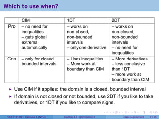
  • 12. Which to use when? CIM 1DT 2DT Pro – no need for – works on – works on inequalities non-closed, non-closed, – gets global non-bounded non-bounded extrema intervals intervals automatically – only one derivative – no need for inequalities Con – only for closed – Uses inequalities – More derivatives bounded intervals – More work at – less conclusive boundary than CIM than 1DT – more work at boundary than CIM . . . . . . V63.0121.021, Calculus I (NYU) Section 4.5 Optimization II class supplement 9 / 25
  • 13. Which to use when? CIM 1DT 2DT Pro – no need for – works on – works on inequalities non-closed, non-closed, – gets global non-bounded non-bounded extrema intervals intervals automatically – only one derivative – no need for inequalities Con – only for closed – Uses inequalities – More derivatives bounded intervals – More work at – less conclusive boundary than CIM than 1DT – more work at boundary than CIM Use CIM if it applies: the domain is a closed, bounded interval If domain is not closed or not bounded, use 2DT if you like to take derivatives, or 1DT if you like to compare signs. . . . . . . V63.0121.021, Calculus I (NYU) Section 4.5 Optimization II class supplement 9 / 25
  • 14. Outline Recall More examples Addition Distance Triangles Economics The Statue of Liberty . . . . . . V63.0121.021, Calculus I (NYU) Section 4.5 Optimization II class supplement 10 / 25
  • 15. Addition with a constraint Example Find two positive numbers x and y with xy = 16 and x + y as small as possible. . . . . . . V63.0121.021, Calculus I (NYU) Section 4.5 Optimization II class supplement 11 / 25
  • 16. Addition with a constraint Example Find two positive numbers x and y with xy = 16 and x + y as small as possible. Solution Objective: minimize S = x + y subject to the constraint that xy = 16 . . . . . . V63.0121.021, Calculus I (NYU) Section 4.5 Optimization II class supplement 11 / 25
  • 17. Addition with a constraint Example Find two positive numbers x and y with xy = 16 and x + y as small as possible. Solution Objective: minimize S = x + y subject to the constraint that xy = 16 Eliminate y: y = 16/x so S = x + 16/x. The domain of consideration is (0, ∞). . . . . . . V63.0121.021, Calculus I (NYU) Section 4.5 Optimization II class supplement 11 / 25
  • 18. Addition with a constraint Example Find two positive numbers x and y with xy = 16 and x + y as small as possible. Solution Objective: minimize S = x + y subject to the constraint that xy = 16 Eliminate y: y = 16/x so S = x + 16/x. The domain of consideration is (0, ∞). Find the critical points: S′ (x) = 1 − 16/x2 , which is 0 when x = 4. . . . . . . V63.0121.021, Calculus I (NYU) Section 4.5 Optimization II class supplement 11 / 25
  • 19. Addition with a constraint Example Find two positive numbers x and y with xy = 16 and x + y as small as possible. Solution Objective: minimize S = x + y subject to the constraint that xy = 16 Eliminate y: y = 16/x so S = x + 16/x. The domain of consideration is (0, ∞). Find the critical points: S′ (x) = 1 − 16/x2 , which is 0 when x = 4. Classify the critical points: S′′ (x) = 32/x3 , which is always positive. So the graph is always concave up, 4 is a local min, and therefore the global min. . . . . . . V63.0121.021, Calculus I (NYU) Section 4.5 Optimization II class supplement 11 / 25
  • 20. Addition with a constraint Example Find two positive numbers x and y with xy = 16 and x + y as small as possible. Solution Objective: minimize S = x + y subject to the constraint that xy = 16 Eliminate y: y = 16/x so S = x + 16/x. The domain of consideration is (0, ∞). Find the critical points: S′ (x) = 1 − 16/x2 , which is 0 when x = 4. Classify the critical points: S′′ (x) = 32/x3 , which is always positive. So the graph is always concave up, 4 is a local min, and therefore the global min. So the numbers are x = y = 4, Smin = 8. . . . . . . V63.0121.021, Calculus I (NYU) Section 4.5 Optimization II class supplement 11 / 25
  • 21. Distance Example Find the point P on the parabola y = x2 closest to the point (3, 0). . . . . . . V63.0121.021, Calculus I (NYU) Section 4.5 Optimization II class supplement 12 / 25
  • 22. Distance Example Find the point P on the parabola y = x2 closest to the point (3, 0). Solution y (x, x2 ) . x . . . . 3 . . V63.0121.021, Calculus I (NYU) Section 4.5 Optimization II class supplement 12 / 25
  • 23. Distance Example Find the point P on the parabola y = x2 closest to the point (3, 0). Solution y The distance between (x, x2 ) and (3, 0) is given by √ f(x) = (x − 3)2 + (x2 − 0)2 (x, x2 ) . x . . . . 3 . . V63.0121.021, Calculus I (NYU) Section 4.5 Optimization II class supplement 12 / 25
  • 24. Distance Example Find the point P on the parabola y = x2 closest to the point (3, 0). Solution y The distance between (x, x2 ) and (3, 0) is given by √ f(x) = (x − 3)2 + (x2 − 0)2 We may instead minimize the square of f: g(x) = f(x)2 = (x − 3)2 + x4 (x, x2 ) . x . . . . 3 . . V63.0121.021, Calculus I (NYU) Section 4.5 Optimization II class supplement 12 / 25
  • 25. Distance Example Find the point P on the parabola y = x2 closest to the point (3, 0). Solution y The distance between (x, x2 ) and (3, 0) is given by √ f(x) = (x − 3)2 + (x2 − 0)2 We may instead minimize the square of f: g(x) = f(x)2 = (x − 3)2 + x4 (x, x2 ) . x The domain is (−∞, ∞). . . . . 3 . . V63.0121.021, Calculus I (NYU) Section 4.5 Optimization II class supplement 12 / 25
  • 26. Distance problem minimization step We want to find the global minimum of g(x) = (x − 3)2 + x4 . . . . . . . V63.0121.021, Calculus I (NYU) Section 4.5 Optimization II class supplement 13 / 25
  • 27. Distance problem minimization step We want to find the global minimum of g(x) = (x − 3)2 + x4 . g′ (x) = 2(x − 3) + 4x3 = 4x3 + 2x − 6 = 2(2x3 + x − 3) . . . . . . V63.0121.021, Calculus I (NYU) Section 4.5 Optimization II class supplement 13 / 25
  • 28. Distance problem minimization step We want to find the global minimum of g(x) = (x − 3)2 + x4 . g′ (x) = 2(x − 3) + 4x3 = 4x3 + 2x − 6 = 2(2x3 + x − 3) If a polynomial has integer roots, they are factors of the constant term (Euler) . . . . . . V63.0121.021, Calculus I (NYU) Section 4.5 Optimization II class supplement 13 / 25
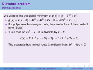
  • 29. Distance problem minimization step We want to find the global minimum of g(x) = (x − 3)2 + x4 . g′ (x) = 2(x − 3) + 4x3 = 4x3 + 2x − 6 = 2(2x3 + x − 3) If a polynomial has integer roots, they are factors of the constant term (Euler) 1 is a root, so 2x3 + x − 3 is divisible by x − 1: f′ (x) = 2(2x3 + x − 3) = 2(x − 1)(2x2 + 2x + 3) The quadratic has no real roots (the discriminant b2 − 4ac < 0) . . . . . . V63.0121.021, Calculus I (NYU) Section 4.5 Optimization II class supplement 13 / 25
  • 30. Distance problem minimization step We want to find the global minimum of g(x) = (x − 3)2 + x4 . g′ (x) = 2(x − 3) + 4x3 = 4x3 + 2x − 6 = 2(2x3 + x − 3) If a polynomial has integer roots, they are factors of the constant term (Euler) 1 is a root, so 2x3 + x − 3 is divisible by x − 1: f′ (x) = 2(2x3 + x − 3) = 2(x − 1)(2x2 + 2x + 3) The quadratic has no real roots (the discriminant b2 − 4ac < 0) We see f′ (1) = 0, f′ (x) < 0 if x < 1, and f′ (x) > 0 if x > 1. So 1 is the global minimum. . . . . . . V63.0121.021, Calculus I (NYU) Section 4.5 Optimization II class supplement 13 / 25
  • 31. Distance problem minimization step We want to find the global minimum of g(x) = (x − 3)2 + x4 . g′ (x) = 2(x − 3) + 4x3 = 4x3 + 2x − 6 = 2(2x3 + x − 3) If a polynomial has integer roots, they are factors of the constant term (Euler) 1 is a root, so 2x3 + x − 3 is divisible by x − 1: f′ (x) = 2(2x3 + x − 3) = 2(x − 1)(2x2 + 2x + 3) The quadratic has no real roots (the discriminant b2 − 4ac < 0) We see f′ (1) = 0, f′ (x) < 0 if x < 1, and f′ (x) > 0 if x > 1. So 1 is the global minimum. The point on the parabola closest to (3, 0) is (1, 1). The minimum √ distance is 5. . . . . . . V63.0121.021, Calculus I (NYU) Section 4.5 Optimization II class supplement 13 / 25
  • 32. Remark We’ve used each of the methods (CIM, 1DT, 2DT) so far. Notice how we argued that the critical points were absolute extremes even though 1DT and 2DT only tell you relative/local extremes. . . . . . . V63.0121.021, Calculus I (NYU) Section 4.5 Optimization II class supplement 14 / 25
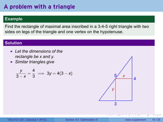
  • 33. A problem with a triangle . Example Find the rectangle of maximal area inscribed in a 3-4-5 right triangle with two sides on legs of the triangle and one vertex on the hypotenuse. Solution 5 4 . 3 . . . . . . V63.0121.021, Calculus I (NYU) Section 4.5 Optimization II class supplement 15 / 25
  • 34. A problem with a triangle . Example Find the rectangle of maximal area inscribed in a 3-4-5 right triangle with two sides on legs of the triangle and one vertex on the hypotenuse. Solution Let the dimensions of the rectangle be x and y. 5 x 4 y . 3 . . . . . . V63.0121.021, Calculus I (NYU) Section 4.5 Optimization II class supplement 15 / 25
  • 35. A problem with a triangle . Example Find the rectangle of maximal area inscribed in a 3-4-5 right triangle with two sides on legs of the triangle and one vertex on the hypotenuse. Solution Let the dimensions of the rectangle be x and y. Similar triangles give y 4 = =⇒ 3y = 4(3 − x) 3−x 3 5 x 4 y . 3 . . . . . . V63.0121.021, Calculus I (NYU) Section 4.5 Optimization II class supplement 15 / 25
  • 36. A problem with a triangle . Example Find the rectangle of maximal area inscribed in a 3-4-5 right triangle with two sides on legs of the triangle and one vertex on the hypotenuse. Solution Let the dimensions of the rectangle be x and y. Similar triangles give y 4 = =⇒ 3y = 4(3 − x) 3−x 3 5 x 4 4 So y = 4 − x and y 3 ( ) 4 4 . A(x) = x 4 − x = 4x − x2 3 3 3 . . . . . . V63.0121.021, Calculus I (NYU) Section 4.5 Optimization II class supplement 15 / 25
  • 37. Triangle Problem maximization step 4 We want to find the absolute maximum of A(x) = 4x − x2 on the 3 interval [0, 3]. . . . . . . V63.0121.021, Calculus I (NYU) Section 4.5 Optimization II class supplement 16 / 25
  • 38. Triangle Problem maximization step 4 We want to find the absolute maximum of A(x) = 4x − x2 on the 3 interval [0, 3]. A(0) = A(3) = 0 . . . . . . V63.0121.021, Calculus I (NYU) Section 4.5 Optimization II class supplement 16 / 25
  • 39. Triangle Problem maximization step 4 We want to find the absolute maximum of A(x) = 4x − x2 on the 3 interval [0, 3]. A(0) = A(3) = 0 8 12 A′ (x) = 4 − x, which is zero when x = = 1.5. 3 8 . . . . . . V63.0121.021, Calculus I (NYU) Section 4.5 Optimization II class supplement 16 / 25
  • 40. Triangle Problem maximization step 4 We want to find the absolute maximum of A(x) = 4x − x2 on the 3 interval [0, 3]. A(0) = A(3) = 0 8 12 A′ (x) = 4 − x, which is zero when x = = 1.5. 3 8 Since A(1.5) = 3, this is the absolute maximum. . . . . . . V63.0121.021, Calculus I (NYU) Section 4.5 Optimization II class supplement 16 / 25
  • 41. Triangle Problem maximization step 4 We want to find the absolute maximum of A(x) = 4x − x2 on the 3 interval [0, 3]. A(0) = A(3) = 0 8 12 A′ (x) = 4 − x, which is zero when x = = 1.5. 3 8 Since A(1.5) = 3, this is the absolute maximum. So the dimensions of the rectangle of maximal area are 1.5 × 2. . . . . . . V63.0121.021, Calculus I (NYU) Section 4.5 Optimization II class supplement 16 / 25
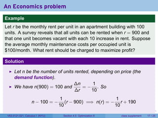
  • 42. An Economics problem Example Let r be the monthly rent per unit in an apartment building with 100 units. A survey reveals that all units can be rented when r = 900 and that one unit becomes vacant with each 10 increase in rent. Suppose the average monthly maintenance costs per occupied unit is $100/month. What rent should be charged to maximize profit? . . . . . . V63.0121.021, Calculus I (NYU) Section 4.5 Optimization II class supplement 17 / 25
  • 43. An Economics problem Example Let r be the monthly rent per unit in an apartment building with 100 units. A survey reveals that all units can be rented when r = 900 and that one unit becomes vacant with each 10 increase in rent. Suppose the average monthly maintenance costs per occupied unit is $100/month. What rent should be charged to maximize profit? Solution Let n be the number of units rented, depending on price (the demand function). ∆n 1 We have n(900) = 100 and = − . So ∆r 10 1 1 n − 100 = − (r − 900) =⇒ n(r) = − r + 190 10 10 . . . . . . V63.0121.021, Calculus I (NYU) Section 4.5 Optimization II class supplement 17 / 25
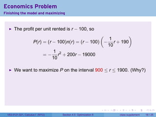
  • 44. Economics Problem Finishing the model and maximizing The profit per unit rented is r − 100, so ( ) 1 P(r) = (r − 100)n(r) = (r − 100) − r + 190 10 1 2 = − r + 200r − 19000 10 . . . . . . V63.0121.021, Calculus I (NYU) Section 4.5 Optimization II class supplement 18 / 25
  • 45. Economics Problem Finishing the model and maximizing The profit per unit rented is r − 100, so ( ) 1 P(r) = (r − 100)n(r) = (r − 100) − r + 190 10 1 2 = − r + 200r − 19000 10 We want to maximize P on the interval 900 ≤ r ≤ 1900. (Why?) . . . . . . V63.0121.021, Calculus I (NYU) Section 4.5 Optimization II class supplement 18 / 25
  • 46. Economics Problem Finishing the model and maximizing The profit per unit rented is r − 100, so ( ) 1 P(r) = (r − 100)n(r) = (r − 100) − r + 190 10 1 2 = − r + 200r − 19000 10 We want to maximize P on the interval 900 ≤ r ≤ 1900. (Why?) A(900) = $800 × 100 = $80, 000, A(1900) = 0 . . . . . . V63.0121.021, Calculus I (NYU) Section 4.5 Optimization II class supplement 18 / 25
  • 47. Economics Problem Finishing the model and maximizing The profit per unit rented is r − 100, so ( ) 1 P(r) = (r − 100)n(r) = (r − 100) − r + 190 10 1 2 = − r + 200r − 19000 10 We want to maximize P on the interval 900 ≤ r ≤ 1900. (Why?) A(900) = $800 × 100 = $80, 000, A(1900) = 0 1 A′ (x) = − r + 200, which is zero when r = 1000. 5 . . . . . . V63.0121.021, Calculus I (NYU) Section 4.5 Optimization II class supplement 18 / 25
  • 48. Economics Problem Finishing the model and maximizing The profit per unit rented is r − 100, so ( ) 1 P(r) = (r − 100)n(r) = (r − 100) − r + 190 10 1 2 = − r + 200r − 19000 10 We want to maximize P on the interval 900 ≤ r ≤ 1900. (Why?) A(900) = $800 × 100 = $80, 000, A(1900) = 0 1 A′ (x) = − r + 200, which is zero when r = 1000. 5 n(1000) = 90, so P(r) = $900 × 90 = $81, 000. This is the maximum intake. . . . . . . V63.0121.021, Calculus I (NYU) Section 4.5 Optimization II class supplement 18 / 25
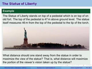
  • 49. The Statue of Liberty Example The Statue of Liberty stands on top of a pedestal which is on top of on old fort. The top of the pedestal is 47 m above ground level. The statue itself measures 46 m from the top of the pedestal to the tip of the torch. What distance should one stand away from the statue in order to maximize the view of the statue? That is, what distance will maximize the portion of the viewer’s vision taken up by the statue? . . . . . . V63.0121.021, Calculus I (NYU) Section 4.5 Optimization II class supplement 19 / 25
  • 50. The Statue of Liberty Seting up the model Solution The angle subtended by the a statue in the viewer’s eye can be expressed as ( ) ( ) b a+b b θ θ = arctan −arctan . x x x The domain of θ is all positive real numbers x. . . . . . . V63.0121.021, Calculus I (NYU) Section 4.5 Optimization II class supplement 20 / 25
  • 51. The Statue of Liberty Finding the derivative ( ) ( ) a+b b θ = arctan − arctan x x So dθ 1 −(a + b) 1 −b = ( )2 · − ( )2 · 2 dx a+b x2 b x 1+ x 1+ x b a+b = 2 − x2 + b x2 + (a + b)2 [ 2 ] [ ] x + (a + b)2 b − (a + b) x2 + b2 = [ ] (x2 + b2 ) x2 + (a + b)2 . . . . . . V63.0121.021, Calculus I (NYU) Section 4.5 Optimization II class supplement 21 / 25
  • 52. The Statue of Liberty Finding the critical points [ 2 ] [ ] dθ x + (a + b)2 b − (a + b) x2 + b2 = [ ] dx (x2 + b2 ) x2 + (a + b)2 . . . . . . V63.0121.021, Calculus I (NYU) Section 4.5 Optimization II class supplement 22 / 25
  • 53. The Statue of Liberty Finding the critical points [ 2 ] [ ] dθ x + (a + b)2 b − (a + b) x2 + b2 = [ ] dx (x2 + b2 ) x2 + (a + b)2 This derivative is zero if and only if the numerator is zero, so we seek x such that [ ] [ ] 0 = x2 + (a + b)2 b − (a + b) x2 + b2 = a(ab + b2 − x2 ) . . . . . . V63.0121.021, Calculus I (NYU) Section 4.5 Optimization II class supplement 22 / 25
  • 54. The Statue of Liberty Finding the critical points [ 2 ] [ ] dθ x + (a + b)2 b − (a + b) x2 + b2 = [ ] dx (x2 + b2 ) x2 + (a + b)2 This derivative is zero if and only if the numerator is zero, so we seek x such that [ ] [ ] 0 = x2 + (a + b)2 b − (a + b) x2 + b2 = a(ab + b2 − x2 ) √ The only positive solution is x = b(a + b). . . . . . . V63.0121.021, Calculus I (NYU) Section 4.5 Optimization II class supplement 22 / 25
  • 55. The Statue of Liberty Finding the critical points [ 2 ] [ ] dθ x + (a + b)2 b − (a + b) x2 + b2 = [ ] dx (x2 + b2 ) x2 + (a + b)2 This derivative is zero if and only if the numerator is zero, so we seek x such that [ ] [ ] 0 = x2 + (a + b)2 b − (a + b) x2 + b2 = a(ab + b2 − x2 ) √ The only positive solution is x = b(a + b). Using the first derivative test, we see that dθ/dx > 0 if √ √ 0 < x < b(a + b) and dθ/dx < 0 if x > b(a + b). So this is definitely the absolute maximum on (0, ∞). . . . . . . V63.0121.021, Calculus I (NYU) Section 4.5 Optimization II class supplement 22 / 25
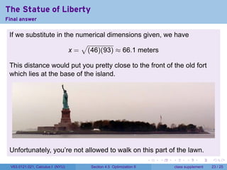
  • 56. The Statue of Liberty Final answer If we substitute in the numerical dimensions given, we have √ x = (46)(93) ≈ 66.1 meters This distance would put you pretty close to the front of the old fort which lies at the base of the island. Unfortunately, you’re not allowed to walk on this part of the lawn. . . . . . . V63.0121.021, Calculus I (NYU) Section 4.5 Optimization II class supplement 23 / 25
  • 57. The Statue of Liberty Discussion √ The length b(a + b) is the geometric mean of the two distances measured from the ground—to the top of the pedestal (a) and the top of the statue (a + b). The geometric mean is of two numbers is always between them and greater than or equal to their average. . . . . . . V63.0121.021, Calculus I (NYU) Section 4.5 Optimization II class supplement 24 / 25
  • 58. Summary Name [_ Problem Solving Strategy Draw a Picture Kathy had a box of 8 crayons. She gave some crayons away. She has 5 left. How many crayons did Kathy give away? Remember the checklist UNDERSTAND What do you want to find out? • Draw a line under the question. Ask yourself: what is the objective? You can draw a picture to solve the problem. Remember your geometry: What number do I add to 5 to get 8? 8 - = 5 similar triangles crayons 5 + 3 = 8 right triangles CHECK Does your answer make sense? trigonometric functions Explain. What number Draw a picture to solve the problem. do I add to 3 Write how many were given away. to make 10? I. I had 10 pencils. ft ft ft A I gave some away. 13 ill i :i I '•' I I I have 3 left. How many i? « 11 I pencils did I give away? I H 11 M i l ~7 U U U U> U U . . . . . . V63.0121.021, Calculus I (NYU) Section 4.5 Optimization II class supplement 25 / 25