SlideShare a Scribd company logo
Section 4.5
              Optimization Problems

                     V63.0121.021, Calculus I

                          New York University


                       November 23, 2010


Announcements

   Turn in HW anytime between now and November 24, 2pm
   No Thursday recitation this week
   Quiz 5 on §§4.1–4.4 next week in recitation

                                                .   .   .   .   .   .
Announcements


         Turn in HW anytime
         between now and
         November 24, 2pm
         No Thursday recitation this
         week
         Quiz 5 on §§4.1–4.4 next
         week in recitation


                                                                      .   .   .      .      .     .

 V63.0121.021, Calculus I (NYU)   Section 4.5 Optimization Problems           November 23, 2010       2 / 31
Objectives


         Given a problem requiring
         optimization, identify the
         objective functions,
         variables, and constraints.
         Solve optimization
         problems with calculus.


                                                                      .   .   .      .      .     .

 V63.0121.021, Calculus I (NYU)   Section 4.5 Optimization Problems           November 23, 2010       3 / 31
Outline


Leading by Example


The Text in the Box


More Examples


                                                                      .   .   .      .      .     .

 V63.0121.021, Calculus I (NYU)   Section 4.5 Optimization Problems           November 23, 2010       4 / 31
Leading by Example


Example
What is the rectangle of fixed perimeter with maximum area?


                                                                      .   .   .      .      .     .

 V63.0121.021, Calculus I (NYU)   Section 4.5 Optimization Problems           November 23, 2010       5 / 31
Leading by Example


Example
What is the rectangle of fixed perimeter with maximum area?

Solution

      Draw a rectangle.


                                    .
                                                  ℓ


                                                                      .   .   .      .      .     .

 V63.0121.021, Calculus I (NYU)   Section 4.5 Optimization Problems           November 23, 2010       5 / 31
Leading by Example


Example
What is the rectangle of fixed perimeter with maximum area?

Solution

      Draw a rectangle.


                                                                      w

                                    .
                                                  ℓ


                                                                      .   .   .      .      .     .

 V63.0121.021, Calculus I (NYU)   Section 4.5 Optimization Problems           November 23, 2010       5 / 31
Solution Continued

      Let its length be ℓ and its width be w. The objective function is
      area A = ℓw.


                                                                      .   .   .      .      .     .

 V63.0121.021, Calculus I (NYU)   Section 4.5 Optimization Problems           November 23, 2010       6 / 31
Solution Continued

      Let its length be ℓ and its width be w. The objective function is
      area A = ℓw.
      This is a function of two variables, not one. But the perimeter is
      fixed.
                                         p − 2w
      Since p = 2ℓ + 2w, we have ℓ =            ,
                                            2


                                                                      .   .   .      .      .     .

 V63.0121.021, Calculus I (NYU)   Section 4.5 Optimization Problems           November 23, 2010       6 / 31
Solution Continued

      Let its length be ℓ and its width be w. The objective function is
      area A = ℓw.
      This is a function of two variables, not one. But the perimeter is
      fixed.
                                         p − 2w
      Since p = 2ℓ + 2w, we have ℓ =            , so
                                            2
                                  p − 2w      1             1
                   A = ℓw =              · w = (p − 2w)(w) = pw − w2
                                     2        2             2


                                                                        .   .   .      .      .     .

 V63.0121.021, Calculus I (NYU)     Section 4.5 Optimization Problems           November 23, 2010       6 / 31
Solution Continued

      Let its length be ℓ and its width be w. The objective function is
      area A = ℓw.
      This is a function of two variables, not one. But the perimeter is
      fixed.
                                         p − 2w
      Since p = 2ℓ + 2w, we have ℓ =            , so
                                            2
                                  p − 2w      1             1
                   A = ℓw =              · w = (p − 2w)(w) = pw − w2
                                     2        2             2


      Now we have A as a function of w alone (p is constant).
      The natural domain of this function is [0, p/2] (we want to make
      sure A(w) ≥ 0).

                                                                        .   .   .      .      .     .

 V63.0121.021, Calculus I (NYU)     Section 4.5 Optimization Problems           November 23, 2010       6 / 31
Solution Concluded

                                                                          1
We use the Closed Interval Method for A(w) =                                pw − w2 on [0, p/2].
                                                                          2
      At the endpoints, A(0) = A(p/2) = 0.


                                                                      .      .   .      .      .     .

 V63.0121.021, Calculus I (NYU)   Section 4.5 Optimization Problems              November 23, 2010       7 / 31
Solution Concluded

                                                                          1
We use the Closed Interval Method for A(w) =                                pw − w2 on [0, p/2].
                                                                          2
      At the endpoints, A(0) = A(p/2) = 0.
                                           dA  1
      To find the critical points, we find    = p − 2w.
                                           dw  2
      The critical points are when

                                        1               p
                                  0=      p − 2w =⇒ w =
                                        2               4


      Since this is the only critical point, it must be the maximum. In this
                p
      case ℓ = as well.
                4
      We have a square! The maximal area is A(p/4) = p2 /16.

                                                                      .      .   .      .      .     .

 V63.0121.021, Calculus I (NYU)   Section 4.5 Optimization Problems              November 23, 2010       7 / 31
Outline


Leading by Example


The Text in the Box


More Examples


                                                                      .   .   .      .      .     .

 V63.0121.021, Calculus I (NYU)   Section 4.5 Optimization Problems           November 23, 2010       8 / 31
Strategies for Problem Solving


  1. Understand the problem
  2. Devise a plan
  3. Carry out the plan
  4. Review and extend


                                                                 György Pólya
                                                             (Hungarian, 1887–1985)
                                                                      .   .   .      .      .     .

 V63.0121.021, Calculus I (NYU)   Section 4.5 Optimization Problems           November 23, 2010       9 / 31
The Text in the Box


 1. Understand the Problem. What is known? What is unknown?
    What are the conditions?


                                                                      .   .    .      .      .    .

 V63.0121.021, Calculus I (NYU)   Section 4.5 Optimization Problems           November 23, 2010   10 / 31
The Text in the Box


 1. Understand the Problem. What is known? What is unknown?
    What are the conditions?
 2. Draw a diagram.
 3. Introduce Notation.
 4. Express the “objective function” Q in terms of the other symbols
 5. If Q is a function of more than one “decision variable”, use the
    given information to eliminate all but one of them.
 6. Find the absolute maximum (or minimum, depending on the
    problem) of the function on its domain.


                                                                      .   .    .      .      .    .

 V63.0121.021, Calculus I (NYU)   Section 4.5 Optimization Problems           November 23, 2010   10 / 31
Polya's Method in Kindergarten
                                  Name    [_
                                  Problem Solving Strategy
                                  Draw a Picture
                                         Kathy had a box of 8 crayons.
                                         She gave some crayons away.
                                         She has 5 left.
                                         How many crayons did Kathy give away?

                                   UNDERSTAND
                                                                           •
                                         What do you want to find out?
                                         Draw a line under the question.


                                         You can draw a picture
                                         to solve the problem.


                                                                                     What number do I
                                                                                     add to 5 to get 8?
                                                                                        8 -     = 5
                                                                           crayons     5 + 3 = 8

                                   CHECK
                                         Does your answer make sense?
                                         Explain.
                                                                                 What number
                                         Draw a picture to solve the problem.   do I add to 3
                                         Write how many were given away.         to make 10?

                                         I. I had 10 pencils.                             ft   ft                ft   A
                                            I gave some away.                         13 ill
                                                                                      i   :i
                                                                                                    I
                                                                                                    '•'        I I
                                            I have 3 left. How many                       i?        «
                                                                                          11        I

                                            pencils did I give away?                                I
                                                                                                          .   H 11
                                                                                                                          .    .      .      .    .
                                                                                                              M i l

 V63.0121.021, Calculus I (NYU)                ~7 Section 4.5 Optimization Problems
                                                                                 U U           U U> U U
                                                                                                                              November 23, 2010   11 / 31
Recall: The Closed Interval Method
See Section 4.1


The Closed Interval Method
To find the extreme values of a function f on [a, b], we need to:
       Evaluate f at the endpoints a and b
       Evaluate f at the critical points x where either f′ (x) = 0 or f is not
       differentiable at x.
       The points with the largest function value are the global maximum
       points
       The points with the smallest/most negative function value are the
       global minimum points.


                                                                       .   .    .      .      .    .

  V63.0121.021, Calculus I (NYU)   Section 4.5 Optimization Problems           November 23, 2010   12 / 31
Recall: The First Derivative Test
See Section 4.3

Theorem (The First Derivative Test)
Let f be continuous on (a, b) and c a critical point of f in (a, b).
       If f′ changes from negative to positive at c, then c is a local
       minimum.
       If f′ changes from positive to negative at c, then c is a local
       maximum.
       If f′ does not change sign at c, then c is not a local extremum.


                                                                       .   .    .      .      .    .

  V63.0121.021, Calculus I (NYU)   Section 4.5 Optimization Problems           November 23, 2010   13 / 31
Recall: The First Derivative Test
See Section 4.3

Theorem (The First Derivative Test)
Let f be continuous on (a, b) and c a critical point of f in (a, b).
       If f′ changes from negative to positive at c, then c is a local
       minimum.
       If f′ changes from positive to negative at c, then c is a local
       maximum.
       If f′ does not change sign at c, then c is not a local extremum.

Corollary

       If f′ < 0 for all x < c and f′ (x) > 0 for all x > c, then c is the global
       minimum of f on (a, b).
       If f′ < 0 for all x > c and f′ (x) > 0 for all x < c, then c is the global
       maximum of f on (a, b).
                                                                       .   .    .      .      .    .

  V63.0121.021, Calculus I (NYU)   Section 4.5 Optimization Problems           November 23, 2010   13 / 31
Recall: The Second Derivative Test
See Section 4.3

Theorem (The Second Derivative Test)
Let f, f′ , and f′′ be continuous on [a, b]. Let c be in (a, b) with f′ (c) = 0.
       If f′′ (c) < 0, then f(c) is a local maximum.
       If f′′ (c) > 0, then f(c) is a local minimum.


                                                                       .   .    .      .      .    .

  V63.0121.021, Calculus I (NYU)   Section 4.5 Optimization Problems           November 23, 2010   14 / 31
Recall: The Second Derivative Test
See Section 4.3

Theorem (The Second Derivative Test)
Let f, f′ , and f′′ be continuous on [a, b]. Let c be in (a, b) with f′ (c) = 0.
       If f′′ (c) < 0, then f(c) is a local maximum.
       If f′′ (c) > 0, then f(c) is a local minimum.

Warning
If f′′ (c) = 0, the second derivative test is inconclusive (this does not
mean c is neither; we just don’t know yet).

Corollary

       If f′ (c) = 0 and f′′ (x) > 0 for all x, then c is the global minimum of f
       If f′ (c) = 0 and f′′ (x) < 0 for all x, then c is the global maximum of f
                                                                       .   .    .      .      .    .

  V63.0121.021, Calculus I (NYU)   Section 4.5 Optimization Problems           November 23, 2010   14 / 31
Which to use when?

            CIM                         1DT                               2DT
 Pro        – no need for               – works on                        – works on
            inequalities                non-closed,                       non-closed,
            – gets global               non-bounded                       non-bounded
            extrema                     intervals                         intervals
            automatically               – only one derivative             – no need for
                                                                          inequalities
 Con        – only for closed           – Uses inequalities               – More derivatives
            bounded intervals           – More work at                    – less conclusive
                                        boundary than CIM                 than 1DT
                                                                          – more work at
                                                                          boundary than CIM


                                                                      .   .    .      .      .    .

 V63.0121.021, Calculus I (NYU)   Section 4.5 Optimization Problems           November 23, 2010   15 / 31
Which to use when?

            CIM                         1DT                               2DT
 Pro        – no need for               – works on                        – works on
            inequalities                non-closed,                       non-closed,
            – gets global               non-bounded                       non-bounded
            extrema                     intervals                         intervals
            automatically               – only one derivative             – no need for
                                                                          inequalities
 Con        – only for closed           – Uses inequalities               – More derivatives
            bounded intervals           – More work at                    – less conclusive
                                        boundary than CIM                 than 1DT
                                                                          – more work at
                                                                          boundary than CIM

      Use CIM if it applies: the domain is a closed, bounded interval
      If domain is not closed or not bounded, use 2DT if you like to take
      derivatives, or 1DT if you like to compare signs.
                                                                      .   .    .      .      .    .

 V63.0121.021, Calculus I (NYU)   Section 4.5 Optimization Problems           November 23, 2010   15 / 31
Outline


Leading by Example


The Text in the Box


More Examples


                                                                      .   .    .      .      .    .

 V63.0121.021, Calculus I (NYU)   Section 4.5 Optimization Problems           November 23, 2010   16 / 31
Another Example


Example (The Best Fencing Plan)
A rectangular plot of farmland will be bounded on one side by a river
and on the other three sides by a single-strand electric fence. With
800m of wire at your disposal, what is the largest area you can
enclose, and what are its dimensions?


                                                                      .   .    .      .      .    .

 V63.0121.021, Calculus I (NYU)   Section 4.5 Optimization Problems           November 23, 2010   17 / 31
Solution

 1. Everybody understand?


                                                                      .   .    .      .      .    .

 V63.0121.021, Calculus I (NYU)   Section 4.5 Optimization Problems           November 23, 2010   18 / 31
Another Example


Example (The Best Fencing Plan)
A rectangular plot of farmland will be bounded on one side by a river
and on the other three sides by a single-strand electric fence. With
800m of wire at your disposal, what is the largest area you can
enclose, and what are its dimensions?


                                                                      .   .    .      .      .    .

 V63.0121.021, Calculus I (NYU)   Section 4.5 Optimization Problems           November 23, 2010   19 / 31
Another Example


Example (The Best Fencing Plan)
A rectangular plot of farmland will be bounded on one side by a river
and on the other three sides by a single-strand electric fence. With
800m of wire at your disposal, what is the largest area you can
enclose, and what are its dimensions?

      Known: amount of fence used
      Unknown: area enclosed
      Objective: maximize area
      Constraint: fixed fence length


                                                                      .   .    .      .      .    .

 V63.0121.021, Calculus I (NYU)   Section 4.5 Optimization Problems           November 23, 2010   19 / 31
Solution

 1. Everybody understand?


                                                                      .   .    .      .      .    .

 V63.0121.021, Calculus I (NYU)   Section 4.5 Optimization Problems           November 23, 2010   20 / 31
Solution

 1. Everybody understand?
 2. Draw a diagram.


                                                                      .   .    .      .      .    .

 V63.0121.021, Calculus I (NYU)   Section 4.5 Optimization Problems           November 23, 2010   20 / 31
Diagram

A rectangular plot of farmland will be bounded on one side by a river
and on the other three sides by a single-strand electric fence. With 800
m of wire at your disposal, what is the largest area you can enclose,
and what are its dimensions?


                                  .

                                                      .


                                                                          .   .    .      .      .    .

 V63.0121.021, Calculus I (NYU)       Section 4.5 Optimization Problems           November 23, 2010   21 / 31
Solution

 1. Everybody understand?
 2. Draw a diagram.


                                                                      .   .    .      .      .    .

 V63.0121.021, Calculus I (NYU)   Section 4.5 Optimization Problems           November 23, 2010   22 / 31
Solution

 1. Everybody understand?
 2. Draw a diagram.
 3. Length and width are ℓ and w. Length of wire used is p.


                                                                      .   .    .      .      .    .

 V63.0121.021, Calculus I (NYU)   Section 4.5 Optimization Problems           November 23, 2010   22 / 31
Diagram

A rectangular plot of farmland will be bounded on one side by a river
and on the other three sides by a single-strand electric fence. With 800
m of wire at your disposal, what is the largest area you can enclose,
and what are its dimensions?


                                  .

                                                      .


                                                                          .   .    .      .      .    .

 V63.0121.021, Calculus I (NYU)       Section 4.5 Optimization Problems           November 23, 2010   23 / 31
Diagram

A rectangular plot of farmland will be bounded on one side by a river
and on the other three sides by a single-strand electric fence. With 800
m of wire at your disposal, what is the largest area you can enclose,
and what are its dimensions?
                                                         ℓ


                                  w

                                      .

                                                          .


                                                                              .   .    .      .      .    .

 V63.0121.021, Calculus I (NYU)           Section 4.5 Optimization Problems           November 23, 2010   23 / 31
Solution

 1. Everybody understand?
 2. Draw a diagram.
 3. Length and width are ℓ and w. Length of wire used is p.


                                                                      .   .    .      .      .    .

 V63.0121.021, Calculus I (NYU)   Section 4.5 Optimization Problems           November 23, 2010   24 / 31
Solution

 1. Everybody understand?
 2. Draw a diagram.
 3. Length and width are ℓ and w. Length of wire used is p.
 4. Q = area = ℓw.
 5. Since p = ℓ + 2w, we have ℓ = p − 2w and so

                                  Q(w) = (p − 2w)(w) = pw − 2w2

      The domain of Q is [0, p/2]


                                                                         .   .    .      .      .    .

 V63.0121.021, Calculus I (NYU)      Section 4.5 Optimization Problems           November 23, 2010   24 / 31
Solution

 1. Everybody understand?
 2. Draw a diagram.
 3. Length and width are ℓ and w. Length of wire used is p.
 4. Q = area = ℓw.
 5. Since p = ℓ + 2w, we have ℓ = p − 2w and so

                                  Q(w) = (p − 2w)(w) = pw − 2w2

    The domain of Q is [0, p/2]
    dQ                                 p
 6.    = p − 4w, which is zero when w = .
    dw                                 4


                                                                         .   .    .      .      .    .

 V63.0121.021, Calculus I (NYU)      Section 4.5 Optimization Problems           November 23, 2010   24 / 31
Solution

 1. Everybody understand?
 2. Draw a diagram.
 3. Length and width are ℓ and w. Length of wire used is p.
 4. Q = area = ℓw.
 5. Since p = ℓ + 2w, we have ℓ = p − 2w and so

                                  Q(w) = (p − 2w)(w) = pw − 2w2

    The domain of Q is [0, p/2]
    dQ                                 p
 6.    = p − 4w, which is zero when w = . Q(0) = Q(p/2) = 0, but
    dw                                 4
                              (p)            p     p2   p2
                          Q           =p·      −2·    =    = 80, 000m2
                                  4          4     16   8
      so the critical point is the absolute maximum.
                                                                           .   .    .      .      .    .

 V63.0121.021, Calculus I (NYU)        Section 4.5 Optimization Problems           November 23, 2010   24 / 31
Your turn

Example (The shortest fence)
A 216m2 rectangular pea patch is to be enclosed by a fence and
divided into two equal parts by another fence parallel to one of its
sides. What dimensions for the outer rectangle will require the smallest
total length of fence? How much fence will be needed?


                                                                      .   .    .      .      .    .

 V63.0121.021, Calculus I (NYU)   Section 4.5 Optimization Problems           November 23, 2010   25 / 31
Your turn

Example (The shortest fence)
A 216m2 rectangular pea patch is to be enclosed by a fence and
divided into two equal parts by another fence parallel to one of its
sides. What dimensions for the outer rectangle will require the smallest
total length of fence? How much fence will be needed?

Solution
Let the length and width of the pea patch be ℓ and w. The amount of
fence needed is f = 2ℓ + 3w. Since ℓw = A, a constant, we have
                                                  A
                                    f(w) = 2        + 3w.
                                                  w
The domain is all positive numbers.

                                                                      .   .    .      .      .    .

 V63.0121.021, Calculus I (NYU)   Section 4.5 Optimization Problems           November 23, 2010   25 / 31
Diagram


                          w


                                  .
                                                        ℓ

                             f = 2ℓ + 3w                    A = ℓw ≡ 216


                                                                          .   .    .      .      .    .

 V63.0121.021, Calculus I (NYU)       Section 4.5 Optimization Problems           November 23, 2010   26 / 31
Solution (Continued)
                                                                          2A
 We need to find the minimum value of f(w) =                                 + 3w on (0, ∞).
                                                                          w


                                                                      .      .    .      .      .    .

 V63.0121.021, Calculus I (NYU)   Section 4.5 Optimization Problems              November 23, 2010   27 / 31
Solution (Continued)
                                                                          2A
 We need to find the minimum value of f(w) =                                 + 3w on (0, ∞).
                                                                          w
      We have
                              df    2A
                                  =− 2 +3
                              dw    w
                             √
                               2A
      which is zero when w =      .
                                3


                                                                      .      .    .      .      .    .

 V63.0121.021, Calculus I (NYU)   Section 4.5 Optimization Problems              November 23, 2010   27 / 31
Solution (Continued)
                                                                          2A
 We need to find the minimum value of f(w) =                                 + 3w on (0, ∞).
                                                                          w
      We have
                                 df        2A
                                      =− 2 +3
                                 dw        w
                                √
                                   2A
      which is zero when w =           .
                                    3
      Since f′′ (w) = 4Aw−3 , which is positive for all positive w, the
      critical point is a minimum, in fact the global minimum.


                                                                      .      .    .      .      .    .

 V63.0121.021, Calculus I (NYU)   Section 4.5 Optimization Problems              November 23, 2010   27 / 31
Solution (Continued)
                                                                          2A
 We need to find the minimum value of f(w) =                                 + 3w on (0, ∞).
                                                                          w
      We have
                                  df        2A
                                      =− 2 +3
                                  dw        w
                                 √
                                   2A
      which is zero when w =           .
                                    3
      Since f′′ (w) = 4Aw−3 , which is positive for all positive w, the
      critical point is a minimum, in fact the global minimum.
                                              √
                                                2A
      So the area is minimized when w =            = 12 and
                 √                               3
            A      3A
      ℓ= =              = 18. The amount of fence needed is
            w        2
            (√ )            √        √
                2A            3A         2A     √        √
          f            =2·       +3          = 2 6A = 2 6 · 216 = 72m
                 3             2          3                           .      .    .      .      .    .

 V63.0121.021, Calculus I (NYU)   Section 4.5 Optimization Problems              November 23, 2010   27 / 31
Try this one


Example
An advertisement consists of a rectangular printed region plus 1 in
margins on the sides and 1.5 in margins on the top and bottom. If the
total area of the advertisement is to be 120 in2 , what dimensions should
the advertisement be to maximize the area of the printed region?


                                                                      .   .    .      .      .    .

 V63.0121.021, Calculus I (NYU)   Section 4.5 Optimization Problems           November 23, 2010   28 / 31
Try this one


Example
An advertisement consists of a rectangular printed region plus 1 in
margins on the sides and 1.5 in margins on the top and bottom. If the
total area of the advertisement is to be 120 in2 , what dimensions should
the advertisement be to maximize the area of the printed region?

Answer
                                  √         √
The optimal paper dimensions are 4 5 in by 6 5 in.


                                                                      .   .    .      .      .    .

 V63.0121.021, Calculus I (NYU)   Section 4.5 Optimization Problems           November 23, 2010   28 / 31
Solution
Let the dimensions of the
printed region be x and y, P                                                      1.5 cm
the printed area, and A the                                           Lorem ipsum dolor sit amet,
                                                                      consectetur adipiscing elit. Nam
paper area. We wish to                                                dapibus vehicula mollis. Proin nec
                                                                      tristique mi.      Pellentesque quis
maximize P = xy subject to                                            placerat dolor. Praesent a nisl diam.
the constraint that                                                   Phasellus ut elit eu ligula accumsan
                                                                      euismod.        Nunc condimentum
                                                                      lacinia risus a sodales. Morbi nunc
                                                                      risus, tincidunt in tristique sit amet,
  A = (x + 2)(y + 3) ≡ 120


                                                           1 cm


                                                                                                                1 cm
                                                    y                 ultrices eu eros. Proin pellentesque
                                                                      aliquam nibh ut lobortis.         Ut et
                                                                      sollicitudin ipsum.      Proin gravida
Isolating y in A ≡ 120 gives                                          ligula eget odio molestie rhoncus
                                                                      sed nec massa. In ante lorem,
     120                                                              imperdiet eget tincidunt at, pharetra
y=         − 3 which yields                                           sit amet felis.      Nunc nisi velit,
     x+2                                                              tempus ac suscipit quis, blandit
                                                                      vitae mauris. Vestibulum ante ipsum
       (          )                                                   primis in faucibus orci luctus et
         120           120x                                       .   ultrices posuere cubilia Curae;
P=x            −3 =          −3x
         x+2           x+2                                                        1.5 cm
The domain of P is (0, ∞).                                                              x
                                                                           .        .        .       .          .      .

 V63.0121.021, Calculus I (NYU)   Section 4.5 Optimization Problems                         November 23, 2010          29 / 31
Solution (Concluded)

      We want to find the absolute maximum value of P.
      dP     (x + 2)(120) − (120x)(1)            240 − 3(x + 2)2
          =                              −3=
      dx              (x + 2)2                      (x + 2)2
      There is a single (positive) critical point when
                                 √
      (x + 2)2 = 80 =⇒ x = 4 5 − 2.
                                         d2 P    −480
      The second derivative is              2
                                              =          , which is negative all
                                         dx     (x + 2)3
      along the domain of P.
                                         ( √     )
      Hence the unique critical point x = 4 5 − 2 cm is the absolute
      maximum of P.
                                       √
      This means the paper width is 4 5 cm, and the paper length is
      120     √
       √ = 6 5 cm.
      4 5

                                                                      .   .    .      .      .    .

 V63.0121.021, Calculus I (NYU)   Section 4.5 Optimization Problems           November 23, 2010   30 / 31
Summary

                                                          Name    [_
                                                          Problem Solving Strategy
                                                          Draw a Picture
                                                                 Kathy had a box of 8 crayons.
                                                                 She gave some crayons away.
                                                                 She has 5 left.
                                                                 How many crayons did Kathy give away?


      Remember the checklist                               UNDERSTAND

                                                                 What do you want to find out?
                                                                                                    •


                                                                 Draw a line under the question.
      Ask yourself: what is the
      objective?                                                 You can draw a picture
                                                                 to solve the problem.

      Remember your geometry:
                                                                                                                  What number do I
                                                                                                                  add to 5 to get 8?
                                                                                                                     8 -     = 5
              similar triangles                                                                     crayons         5 + 3 = 8


              right triangles                              CHECK
                                                                 Does your answer make sense?
              trigonometric functions                            Explain.
                                                                                                         What number
                                                                 Draw a picture to solve the problem.   do I add to 3
                                                                 Write how many were given away.         to make 10?

                                                                 I. I had 10 pencils.                                  ft   ft                ft   A
                                                                    I gave some away.                              13 ill
                                                                                                                   i   :i
                                                                                                                                 I
                                                                                                                                 '•'        I I
                                                                    I have 3 left. How many                            i?        «
                                                                                                                       11        I

                                                                    pencils did I give away?                                     I
                                                                                                                                           H 11
                                                                                                                                           M i l
                                                                       ~7                                          U U U U> U U


                                                                            .        .          .             .                        .               .

V63.0121.021, Calculus I (NYU)   Section 4.5 Optimization Problems                             November 23, 2010                                       31 / 31

More Related Content

PDF
Lesson 22: Optimization (Section 041 slides)
PDF
Lesson22 -optimization_problems_slides
PDF
Principal Component Analysis for Tensor Analysis and EEG classification
PDF
Program on Quasi-Monte Carlo and High-Dimensional Sampling Methods for Applie...
PDF
A Szemerédi-type theorem for subsets of the unit cube
PDF
Multilinear singular integrals with entangled structure
PDF
Scattering theory analogues of several classical estimates in Fourier analysis
PDF
Density theorems for Euclidean point configurations
Lesson 22: Optimization (Section 041 slides)
Lesson22 -optimization_problems_slides
Principal Component Analysis for Tensor Analysis and EEG classification
Program on Quasi-Monte Carlo and High-Dimensional Sampling Methods for Applie...
A Szemerédi-type theorem for subsets of the unit cube
Multilinear singular integrals with entangled structure
Scattering theory analogues of several classical estimates in Fourier analysis
Density theorems for Euclidean point configurations

What's hot (19)

PDF
A Szemeredi-type theorem for subsets of the unit cube
PDF
Boundedness of the Twisted Paraproduct
PDF
Lesson 26: The Fundamental Theorem of Calculus (Section 041 slides)
PDF
Lesson 26: The Fundamental Theorem of Calculus (handout)
PDF
Estimates for a class of non-standard bilinear multipliers
PDF
Tales on two commuting transformations or flows
PDF
Lesson 19: The Mean Value Theorem (Section 021 handout)
PDF
Program on Quasi-Monte Carlo and High-Dimensional Sampling Methods for Appli...
PDF
Paraproducts with general dilations
PDF
Lesson 26: The Fundamental Theorem of Calculus (Section 021 handout)
PDF
Some Examples of Scaling Sets
PDF
Program on Quasi-Monte Carlo and High-Dimensional Sampling Methods for Applie...
PDF
Density theorems for anisotropic point configurations
PDF
2012 mdsp pr09 pca lda
PDF
On Twisted Paraproducts and some other Multilinear Singular Integrals
PDF
Variants of the Christ-Kiselev lemma and an application to the maximal Fourie...
PDF
Bellman functions and Lp estimates for paraproducts
PDF
2012 mdsp pr10 ica
PDF
A sharp nonlinear Hausdorff-Young inequality for small potentials
A Szemeredi-type theorem for subsets of the unit cube
Boundedness of the Twisted Paraproduct
Lesson 26: The Fundamental Theorem of Calculus (Section 041 slides)
Lesson 26: The Fundamental Theorem of Calculus (handout)
Estimates for a class of non-standard bilinear multipliers
Tales on two commuting transformations or flows
Lesson 19: The Mean Value Theorem (Section 021 handout)
Program on Quasi-Monte Carlo and High-Dimensional Sampling Methods for Appli...
Paraproducts with general dilations
Lesson 26: The Fundamental Theorem of Calculus (Section 021 handout)
Some Examples of Scaling Sets
Program on Quasi-Monte Carlo and High-Dimensional Sampling Methods for Applie...
Density theorems for anisotropic point configurations
2012 mdsp pr09 pca lda
On Twisted Paraproducts and some other Multilinear Singular Integrals
Variants of the Christ-Kiselev lemma and an application to the maximal Fourie...
Bellman functions and Lp estimates for paraproducts
2012 mdsp pr10 ica
A sharp nonlinear Hausdorff-Young inequality for small potentials
Ad

Viewers also liked (20)

PDF
Lesson 22: Optimization II (Section 021 slides)
PDF
Lesson 11: Implicit Differentiation
PDF
Lesson 13: Exponential and Logarithmic Functions (Section 021 slides)
PDF
Lesson 8: Basic Differentiation Rules (Section 41 slides)
PDF
Lesson 12: Linear Approximation
PDF
Lesson18 -maximum_and_minimum_values_slides
PDF
Lesson 14: Derivatives of Exponential and Logarithmic Functions (Section 021 ...
PDF
Lesson 27: Integration by Substitution (Section 041 slides)
PDF
Lesson 28: Integration by Subsitution
PDF
Lesson 26: Evaluating Definite Integrals
PDF
Lesson 1: Functions
PDF
Lesson 10: The Chain Rule (Section 21 slides)
PDF
Lesson 2: A Catalog of Essential Functions
PDF
Lesson 7: The Derivative (Section 21 slide)
PDF
Calculus 45S Slides April 30, 2008
PDF
Lesson 4: Calculating Limits (Section 41 slides)
PDF
cvpr2011: game theory in CVPR part 1
PDF
Numerical analysis m2 l4slides
PDF
Methods from Mathematical Data Mining (Supported by Optimization)
PDF
Lesson 4: Calculating Limits (Section 21 slides)
Lesson 22: Optimization II (Section 021 slides)
Lesson 11: Implicit Differentiation
Lesson 13: Exponential and Logarithmic Functions (Section 021 slides)
Lesson 8: Basic Differentiation Rules (Section 41 slides)
Lesson 12: Linear Approximation
Lesson18 -maximum_and_minimum_values_slides
Lesson 14: Derivatives of Exponential and Logarithmic Functions (Section 021 ...
Lesson 27: Integration by Substitution (Section 041 slides)
Lesson 28: Integration by Subsitution
Lesson 26: Evaluating Definite Integrals
Lesson 1: Functions
Lesson 10: The Chain Rule (Section 21 slides)
Lesson 2: A Catalog of Essential Functions
Lesson 7: The Derivative (Section 21 slide)
Calculus 45S Slides April 30, 2008
Lesson 4: Calculating Limits (Section 41 slides)
cvpr2011: game theory in CVPR part 1
Numerical analysis m2 l4slides
Methods from Mathematical Data Mining (Supported by Optimization)
Lesson 4: Calculating Limits (Section 21 slides)
Ad

Similar to Lesson 22: Optimization (Section 021 slides) (20)

PDF
Lesson 22: Optimization (Section 041 slides)
PDF
Lesson22 -optimization_problems_slides
PDF
Lesson 22: Optimization (Section 021 slides)
PDF
Lesson 22: Optimization I (Section 4 version)
PDF
Lesson 20: Optimization (handout)
PDF
Lesson 24: Optimization
PDF
Lesson 22: Optimization I (Section 10 Version)
PDF
Lesson 24: Optimization
PDF
Lesson 22: Optimization Problems (handout)
PDF
Lesson 19: Optimization Problems
PDF
Lesson 22: Optimization (Section 021 handout)
PDF
Lesson 22: Optimization (Section 041 handout)
PDF
Lesson 22: Optimization Problems (slides)
PDF
Lesson 22: Optimization Problems (slides)
PDF
Lesson 20: (More) Optimization Problems
PDF
Lesson 20: Optimization (slides)
PDF
CRMS Calculus 2010, April 12, 2010
PDF
Lesson 24: Areas, Distances, the Integral (Section 021 handout)
PDF
Lesson 4: Calculating Limits (handout)
PDF
Lesson 4: Calculating Limits (Section 21 slides)
Lesson 22: Optimization (Section 041 slides)
Lesson22 -optimization_problems_slides
Lesson 22: Optimization (Section 021 slides)
Lesson 22: Optimization I (Section 4 version)
Lesson 20: Optimization (handout)
Lesson 24: Optimization
Lesson 22: Optimization I (Section 10 Version)
Lesson 24: Optimization
Lesson 22: Optimization Problems (handout)
Lesson 19: Optimization Problems
Lesson 22: Optimization (Section 021 handout)
Lesson 22: Optimization (Section 041 handout)
Lesson 22: Optimization Problems (slides)
Lesson 20: (More) Optimization Problems
Lesson 20: Optimization (slides)
CRMS Calculus 2010, April 12, 2010
Lesson 24: Areas, Distances, the Integral (Section 021 handout)
Lesson 4: Calculating Limits (handout)
Lesson 4: Calculating Limits (Section 21 slides)

More from Mel Anthony Pepito (20)

PDF
Lesson 16: Inverse Trigonometric Functions
PDF
Lesson 13: Related Rates Problems
PDF
Lesson 14: Derivatives of Logarithmic and Exponential Functions
PDF
Lesson 15: Exponential Growth and Decay
PDF
Lesson 17: Indeterminate Forms and L'Hôpital's Rule
PDF
Lesson 21: Curve Sketching
PDF
Lesson 19: The Mean Value Theorem
PDF
Lesson 25: The Definite Integral
PDF
Lesson 24: Area and Distances
PDF
Lesson 23: Antiderivatives
PDF
Lesson 27: The Fundamental Theorem of Calculus
PDF
Introduction
PDF
Introduction
PDF
Lesson 3: Limits (Section 21 slides)
PDF
Lesson 3: Limits
PDF
Lesson 5: Continuity (Section 41 slides)
PDF
Lesson 5: Continuity (Section 21 slides)
PDF
Lesson 2: A Catalog of Essential Functions
PDF
Lesson 6: Limits Involving ∞ (Section 41 slides)
PDF
Lesson 7: The Derivative (Section 41 slides)
Lesson 16: Inverse Trigonometric Functions
Lesson 13: Related Rates Problems
Lesson 14: Derivatives of Logarithmic and Exponential Functions
Lesson 15: Exponential Growth and Decay
Lesson 17: Indeterminate Forms and L'Hôpital's Rule
Lesson 21: Curve Sketching
Lesson 19: The Mean Value Theorem
Lesson 25: The Definite Integral
Lesson 24: Area and Distances
Lesson 23: Antiderivatives
Lesson 27: The Fundamental Theorem of Calculus
Introduction
Introduction
Lesson 3: Limits (Section 21 slides)
Lesson 3: Limits
Lesson 5: Continuity (Section 41 slides)
Lesson 5: Continuity (Section 21 slides)
Lesson 2: A Catalog of Essential Functions
Lesson 6: Limits Involving ∞ (Section 41 slides)
Lesson 7: The Derivative (Section 41 slides)

Recently uploaded (20)

PDF
Agricultural_Statistics_at_a_Glance_2022_0.pdf
PPTX
Effective Security Operations Center (SOC) A Modern, Strategic, and Threat-In...
PPTX
Digital-Transformation-Roadmap-for-Companies.pptx
PDF
Blue Purple Modern Animated Computer Science Presentation.pdf.pdf
PPT
“AI and Expert System Decision Support & Business Intelligence Systems”
PDF
Peak of Data & AI Encore- AI for Metadata and Smarter Workflows
PDF
Building Integrated photovoltaic BIPV_UPV.pdf
PDF
Advanced methodologies resolving dimensionality complications for autism neur...
PDF
The Rise and Fall of 3GPP – Time for a Sabbatical?
PDF
Encapsulation_ Review paper, used for researhc scholars
PPT
Teaching material agriculture food technology
PDF
Encapsulation theory and applications.pdf
PDF
Profit Center Accounting in SAP S/4HANA, S4F28 Col11
PPTX
Big Data Technologies - Introduction.pptx
PPTX
KOM of Painting work and Equipment Insulation REV00 update 25-dec.pptx
PDF
How UI/UX Design Impacts User Retention in Mobile Apps.pdf
PDF
Review of recent advances in non-invasive hemoglobin estimation
PDF
Dropbox Q2 2025 Financial Results & Investor Presentation
PPTX
Detection-First SIEM: Rule Types, Dashboards, and Threat-Informed Strategy
PPTX
sap open course for s4hana steps from ECC to s4
Agricultural_Statistics_at_a_Glance_2022_0.pdf
Effective Security Operations Center (SOC) A Modern, Strategic, and Threat-In...
Digital-Transformation-Roadmap-for-Companies.pptx
Blue Purple Modern Animated Computer Science Presentation.pdf.pdf
“AI and Expert System Decision Support & Business Intelligence Systems”
Peak of Data & AI Encore- AI for Metadata and Smarter Workflows
Building Integrated photovoltaic BIPV_UPV.pdf
Advanced methodologies resolving dimensionality complications for autism neur...
The Rise and Fall of 3GPP – Time for a Sabbatical?
Encapsulation_ Review paper, used for researhc scholars
Teaching material agriculture food technology
Encapsulation theory and applications.pdf
Profit Center Accounting in SAP S/4HANA, S4F28 Col11
Big Data Technologies - Introduction.pptx
KOM of Painting work and Equipment Insulation REV00 update 25-dec.pptx
How UI/UX Design Impacts User Retention in Mobile Apps.pdf
Review of recent advances in non-invasive hemoglobin estimation
Dropbox Q2 2025 Financial Results & Investor Presentation
Detection-First SIEM: Rule Types, Dashboards, and Threat-Informed Strategy
sap open course for s4hana steps from ECC to s4

Lesson 22: Optimization (Section 021 slides)

  • 1. Section 4.5 Optimization Problems V63.0121.021, Calculus I New York University November 23, 2010 Announcements Turn in HW anytime between now and November 24, 2pm No Thursday recitation this week Quiz 5 on §§4.1–4.4 next week in recitation . . . . . .
  • 2. Announcements Turn in HW anytime between now and November 24, 2pm No Thursday recitation this week Quiz 5 on §§4.1–4.4 next week in recitation . . . . . . V63.0121.021, Calculus I (NYU) Section 4.5 Optimization Problems November 23, 2010 2 / 31
  • 3. Objectives Given a problem requiring optimization, identify the objective functions, variables, and constraints. Solve optimization problems with calculus. . . . . . . V63.0121.021, Calculus I (NYU) Section 4.5 Optimization Problems November 23, 2010 3 / 31
  • 4. Outline Leading by Example The Text in the Box More Examples . . . . . . V63.0121.021, Calculus I (NYU) Section 4.5 Optimization Problems November 23, 2010 4 / 31
  • 5. Leading by Example Example What is the rectangle of fixed perimeter with maximum area? . . . . . . V63.0121.021, Calculus I (NYU) Section 4.5 Optimization Problems November 23, 2010 5 / 31
  • 6. Leading by Example Example What is the rectangle of fixed perimeter with maximum area? Solution Draw a rectangle. . . . . . . . V63.0121.021, Calculus I (NYU) Section 4.5 Optimization Problems November 23, 2010 5 / 31
  • 7. Leading by Example Example What is the rectangle of fixed perimeter with maximum area? Solution Draw a rectangle. . ℓ . . . . . . V63.0121.021, Calculus I (NYU) Section 4.5 Optimization Problems November 23, 2010 5 / 31
  • 8. Leading by Example Example What is the rectangle of fixed perimeter with maximum area? Solution Draw a rectangle. w . ℓ . . . . . . V63.0121.021, Calculus I (NYU) Section 4.5 Optimization Problems November 23, 2010 5 / 31
  • 9. Solution Continued Let its length be ℓ and its width be w. The objective function is area A = ℓw. . . . . . . V63.0121.021, Calculus I (NYU) Section 4.5 Optimization Problems November 23, 2010 6 / 31
  • 10. Solution Continued Let its length be ℓ and its width be w. The objective function is area A = ℓw. This is a function of two variables, not one. But the perimeter is fixed. . . . . . . V63.0121.021, Calculus I (NYU) Section 4.5 Optimization Problems November 23, 2010 6 / 31
  • 11. Solution Continued Let its length be ℓ and its width be w. The objective function is area A = ℓw. This is a function of two variables, not one. But the perimeter is fixed. p − 2w Since p = 2ℓ + 2w, we have ℓ = , 2 . . . . . . V63.0121.021, Calculus I (NYU) Section 4.5 Optimization Problems November 23, 2010 6 / 31
  • 12. Solution Continued Let its length be ℓ and its width be w. The objective function is area A = ℓw. This is a function of two variables, not one. But the perimeter is fixed. p − 2w Since p = 2ℓ + 2w, we have ℓ = , so 2 p − 2w 1 1 A = ℓw = · w = (p − 2w)(w) = pw − w2 2 2 2 . . . . . . V63.0121.021, Calculus I (NYU) Section 4.5 Optimization Problems November 23, 2010 6 / 31
  • 13. Solution Continued Let its length be ℓ and its width be w. The objective function is area A = ℓw. This is a function of two variables, not one. But the perimeter is fixed. p − 2w Since p = 2ℓ + 2w, we have ℓ = , so 2 p − 2w 1 1 A = ℓw = · w = (p − 2w)(w) = pw − w2 2 2 2 Now we have A as a function of w alone (p is constant). . . . . . . V63.0121.021, Calculus I (NYU) Section 4.5 Optimization Problems November 23, 2010 6 / 31
  • 14. Solution Continued Let its length be ℓ and its width be w. The objective function is area A = ℓw. This is a function of two variables, not one. But the perimeter is fixed. p − 2w Since p = 2ℓ + 2w, we have ℓ = , so 2 p − 2w 1 1 A = ℓw = · w = (p − 2w)(w) = pw − w2 2 2 2 Now we have A as a function of w alone (p is constant). The natural domain of this function is [0, p/2] (we want to make sure A(w) ≥ 0). . . . . . . V63.0121.021, Calculus I (NYU) Section 4.5 Optimization Problems November 23, 2010 6 / 31
  • 15. Solution Concluded 1 We use the Closed Interval Method for A(w) = pw − w2 on [0, p/2]. 2 At the endpoints, A(0) = A(p/2) = 0. . . . . . . V63.0121.021, Calculus I (NYU) Section 4.5 Optimization Problems November 23, 2010 7 / 31
  • 16. Solution Concluded 1 We use the Closed Interval Method for A(w) = pw − w2 on [0, p/2]. 2 At the endpoints, A(0) = A(p/2) = 0. dA 1 To find the critical points, we find = p − 2w. dw 2 . . . . . . V63.0121.021, Calculus I (NYU) Section 4.5 Optimization Problems November 23, 2010 7 / 31
  • 17. Solution Concluded 1 We use the Closed Interval Method for A(w) = pw − w2 on [0, p/2]. 2 At the endpoints, A(0) = A(p/2) = 0. dA 1 To find the critical points, we find = p − 2w. dw 2 The critical points are when 1 p 0= p − 2w =⇒ w = 2 4 . . . . . . V63.0121.021, Calculus I (NYU) Section 4.5 Optimization Problems November 23, 2010 7 / 31
  • 18. Solution Concluded 1 We use the Closed Interval Method for A(w) = pw − w2 on [0, p/2]. 2 At the endpoints, A(0) = A(p/2) = 0. dA 1 To find the critical points, we find = p − 2w. dw 2 The critical points are when 1 p 0= p − 2w =⇒ w = 2 4 Since this is the only critical point, it must be the maximum. In this p case ℓ = as well. 4 . . . . . . V63.0121.021, Calculus I (NYU) Section 4.5 Optimization Problems November 23, 2010 7 / 31
  • 19. Solution Concluded 1 We use the Closed Interval Method for A(w) = pw − w2 on [0, p/2]. 2 At the endpoints, A(0) = A(p/2) = 0. dA 1 To find the critical points, we find = p − 2w. dw 2 The critical points are when 1 p 0= p − 2w =⇒ w = 2 4 Since this is the only critical point, it must be the maximum. In this p case ℓ = as well. 4 We have a square! The maximal area is A(p/4) = p2 /16. . . . . . . V63.0121.021, Calculus I (NYU) Section 4.5 Optimization Problems November 23, 2010 7 / 31
  • 20. Outline Leading by Example The Text in the Box More Examples . . . . . . V63.0121.021, Calculus I (NYU) Section 4.5 Optimization Problems November 23, 2010 8 / 31
  • 21. Strategies for Problem Solving 1. Understand the problem 2. Devise a plan 3. Carry out the plan 4. Review and extend György Pólya (Hungarian, 1887–1985) . . . . . . V63.0121.021, Calculus I (NYU) Section 4.5 Optimization Problems November 23, 2010 9 / 31
  • 22. The Text in the Box 1. Understand the Problem. What is known? What is unknown? What are the conditions? . . . . . . V63.0121.021, Calculus I (NYU) Section 4.5 Optimization Problems November 23, 2010 10 / 31
  • 23. The Text in the Box 1. Understand the Problem. What is known? What is unknown? What are the conditions? 2. Draw a diagram. . . . . . . V63.0121.021, Calculus I (NYU) Section 4.5 Optimization Problems November 23, 2010 10 / 31
  • 24. The Text in the Box 1. Understand the Problem. What is known? What is unknown? What are the conditions? 2. Draw a diagram. 3. Introduce Notation. . . . . . . V63.0121.021, Calculus I (NYU) Section 4.5 Optimization Problems November 23, 2010 10 / 31
  • 25. The Text in the Box 1. Understand the Problem. What is known? What is unknown? What are the conditions? 2. Draw a diagram. 3. Introduce Notation. 4. Express the “objective function” Q in terms of the other symbols . . . . . . V63.0121.021, Calculus I (NYU) Section 4.5 Optimization Problems November 23, 2010 10 / 31
  • 26. The Text in the Box 1. Understand the Problem. What is known? What is unknown? What are the conditions? 2. Draw a diagram. 3. Introduce Notation. 4. Express the “objective function” Q in terms of the other symbols 5. If Q is a function of more than one “decision variable”, use the given information to eliminate all but one of them. . . . . . . V63.0121.021, Calculus I (NYU) Section 4.5 Optimization Problems November 23, 2010 10 / 31
  • 27. The Text in the Box 1. Understand the Problem. What is known? What is unknown? What are the conditions? 2. Draw a diagram. 3. Introduce Notation. 4. Express the “objective function” Q in terms of the other symbols 5. If Q is a function of more than one “decision variable”, use the given information to eliminate all but one of them. 6. Find the absolute maximum (or minimum, depending on the problem) of the function on its domain. . . . . . . V63.0121.021, Calculus I (NYU) Section 4.5 Optimization Problems November 23, 2010 10 / 31
  • 28. Polya's Method in Kindergarten Name [_ Problem Solving Strategy Draw a Picture Kathy had a box of 8 crayons. She gave some crayons away. She has 5 left. How many crayons did Kathy give away? UNDERSTAND • What do you want to find out? Draw a line under the question. You can draw a picture to solve the problem. What number do I add to 5 to get 8? 8 - = 5 crayons 5 + 3 = 8 CHECK Does your answer make sense? Explain. What number Draw a picture to solve the problem. do I add to 3 Write how many were given away. to make 10? I. I had 10 pencils. ft ft ft A I gave some away. 13 ill i :i I '•' I I I have 3 left. How many i? « 11 I pencils did I give away? I . H 11 . . . . . M i l V63.0121.021, Calculus I (NYU) ~7 Section 4.5 Optimization Problems U U U U> U U November 23, 2010 11 / 31
  • 29. Recall: The Closed Interval Method See Section 4.1 The Closed Interval Method To find the extreme values of a function f on [a, b], we need to: Evaluate f at the endpoints a and b Evaluate f at the critical points x where either f′ (x) = 0 or f is not differentiable at x. The points with the largest function value are the global maximum points The points with the smallest/most negative function value are the global minimum points. . . . . . . V63.0121.021, Calculus I (NYU) Section 4.5 Optimization Problems November 23, 2010 12 / 31
  • 30. Recall: The First Derivative Test See Section 4.3 Theorem (The First Derivative Test) Let f be continuous on (a, b) and c a critical point of f in (a, b). If f′ changes from negative to positive at c, then c is a local minimum. If f′ changes from positive to negative at c, then c is a local maximum. If f′ does not change sign at c, then c is not a local extremum. . . . . . . V63.0121.021, Calculus I (NYU) Section 4.5 Optimization Problems November 23, 2010 13 / 31
  • 31. Recall: The First Derivative Test See Section 4.3 Theorem (The First Derivative Test) Let f be continuous on (a, b) and c a critical point of f in (a, b). If f′ changes from negative to positive at c, then c is a local minimum. If f′ changes from positive to negative at c, then c is a local maximum. If f′ does not change sign at c, then c is not a local extremum. Corollary If f′ < 0 for all x < c and f′ (x) > 0 for all x > c, then c is the global minimum of f on (a, b). If f′ < 0 for all x > c and f′ (x) > 0 for all x < c, then c is the global maximum of f on (a, b). . . . . . . V63.0121.021, Calculus I (NYU) Section 4.5 Optimization Problems November 23, 2010 13 / 31
  • 32. Recall: The Second Derivative Test See Section 4.3 Theorem (The Second Derivative Test) Let f, f′ , and f′′ be continuous on [a, b]. Let c be in (a, b) with f′ (c) = 0. If f′′ (c) < 0, then f(c) is a local maximum. If f′′ (c) > 0, then f(c) is a local minimum. . . . . . . V63.0121.021, Calculus I (NYU) Section 4.5 Optimization Problems November 23, 2010 14 / 31
  • 33. Recall: The Second Derivative Test See Section 4.3 Theorem (The Second Derivative Test) Let f, f′ , and f′′ be continuous on [a, b]. Let c be in (a, b) with f′ (c) = 0. If f′′ (c) < 0, then f(c) is a local maximum. If f′′ (c) > 0, then f(c) is a local minimum. Warning If f′′ (c) = 0, the second derivative test is inconclusive (this does not mean c is neither; we just don’t know yet). . . . . . . V63.0121.021, Calculus I (NYU) Section 4.5 Optimization Problems November 23, 2010 14 / 31
  • 34. Recall: The Second Derivative Test See Section 4.3 Theorem (The Second Derivative Test) Let f, f′ , and f′′ be continuous on [a, b]. Let c be in (a, b) with f′ (c) = 0. If f′′ (c) < 0, then f(c) is a local maximum. If f′′ (c) > 0, then f(c) is a local minimum. Warning If f′′ (c) = 0, the second derivative test is inconclusive (this does not mean c is neither; we just don’t know yet). Corollary If f′ (c) = 0 and f′′ (x) > 0 for all x, then c is the global minimum of f If f′ (c) = 0 and f′′ (x) < 0 for all x, then c is the global maximum of f . . . . . . V63.0121.021, Calculus I (NYU) Section 4.5 Optimization Problems November 23, 2010 14 / 31
  • 35. Which to use when? CIM 1DT 2DT Pro – no need for – works on – works on inequalities non-closed, non-closed, – gets global non-bounded non-bounded extrema intervals intervals automatically – only one derivative – no need for inequalities Con – only for closed – Uses inequalities – More derivatives bounded intervals – More work at – less conclusive boundary than CIM than 1DT – more work at boundary than CIM . . . . . . V63.0121.021, Calculus I (NYU) Section 4.5 Optimization Problems November 23, 2010 15 / 31
  • 36. Which to use when? CIM 1DT 2DT Pro – no need for – works on – works on inequalities non-closed, non-closed, – gets global non-bounded non-bounded extrema intervals intervals automatically – only one derivative – no need for inequalities Con – only for closed – Uses inequalities – More derivatives bounded intervals – More work at – less conclusive boundary than CIM than 1DT – more work at boundary than CIM Use CIM if it applies: the domain is a closed, bounded interval If domain is not closed or not bounded, use 2DT if you like to take derivatives, or 1DT if you like to compare signs. . . . . . . V63.0121.021, Calculus I (NYU) Section 4.5 Optimization Problems November 23, 2010 15 / 31
  • 37. Outline Leading by Example The Text in the Box More Examples . . . . . . V63.0121.021, Calculus I (NYU) Section 4.5 Optimization Problems November 23, 2010 16 / 31
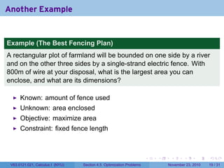
  • 38. Another Example Example (The Best Fencing Plan) A rectangular plot of farmland will be bounded on one side by a river and on the other three sides by a single-strand electric fence. With 800m of wire at your disposal, what is the largest area you can enclose, and what are its dimensions? . . . . . . V63.0121.021, Calculus I (NYU) Section 4.5 Optimization Problems November 23, 2010 17 / 31
  • 39. Solution 1. Everybody understand? . . . . . . V63.0121.021, Calculus I (NYU) Section 4.5 Optimization Problems November 23, 2010 18 / 31
  • 40. Another Example Example (The Best Fencing Plan) A rectangular plot of farmland will be bounded on one side by a river and on the other three sides by a single-strand electric fence. With 800m of wire at your disposal, what is the largest area you can enclose, and what are its dimensions? . . . . . . V63.0121.021, Calculus I (NYU) Section 4.5 Optimization Problems November 23, 2010 19 / 31
  • 41. Another Example Example (The Best Fencing Plan) A rectangular plot of farmland will be bounded on one side by a river and on the other three sides by a single-strand electric fence. With 800m of wire at your disposal, what is the largest area you can enclose, and what are its dimensions? Known: amount of fence used Unknown: area enclosed . . . . . . V63.0121.021, Calculus I (NYU) Section 4.5 Optimization Problems November 23, 2010 19 / 31
  • 42. Another Example Example (The Best Fencing Plan) A rectangular plot of farmland will be bounded on one side by a river and on the other three sides by a single-strand electric fence. With 800m of wire at your disposal, what is the largest area you can enclose, and what are its dimensions? Known: amount of fence used Unknown: area enclosed Objective: maximize area Constraint: fixed fence length . . . . . . V63.0121.021, Calculus I (NYU) Section 4.5 Optimization Problems November 23, 2010 19 / 31
  • 43. Solution 1. Everybody understand? . . . . . . V63.0121.021, Calculus I (NYU) Section 4.5 Optimization Problems November 23, 2010 20 / 31
  • 44. Solution 1. Everybody understand? 2. Draw a diagram. . . . . . . V63.0121.021, Calculus I (NYU) Section 4.5 Optimization Problems November 23, 2010 20 / 31
  • 45. Diagram A rectangular plot of farmland will be bounded on one side by a river and on the other three sides by a single-strand electric fence. With 800 m of wire at your disposal, what is the largest area you can enclose, and what are its dimensions? . . . . . . . . V63.0121.021, Calculus I (NYU) Section 4.5 Optimization Problems November 23, 2010 21 / 31
  • 46. Solution 1. Everybody understand? 2. Draw a diagram. . . . . . . V63.0121.021, Calculus I (NYU) Section 4.5 Optimization Problems November 23, 2010 22 / 31
  • 47. Solution 1. Everybody understand? 2. Draw a diagram. 3. Length and width are ℓ and w. Length of wire used is p. . . . . . . V63.0121.021, Calculus I (NYU) Section 4.5 Optimization Problems November 23, 2010 22 / 31
  • 48. Diagram A rectangular plot of farmland will be bounded on one side by a river and on the other three sides by a single-strand electric fence. With 800 m of wire at your disposal, what is the largest area you can enclose, and what are its dimensions? . . . . . . . . V63.0121.021, Calculus I (NYU) Section 4.5 Optimization Problems November 23, 2010 23 / 31
  • 49. Diagram A rectangular plot of farmland will be bounded on one side by a river and on the other three sides by a single-strand electric fence. With 800 m of wire at your disposal, what is the largest area you can enclose, and what are its dimensions? ℓ w . . . . . . . . V63.0121.021, Calculus I (NYU) Section 4.5 Optimization Problems November 23, 2010 23 / 31
  • 50. Solution 1. Everybody understand? 2. Draw a diagram. 3. Length and width are ℓ and w. Length of wire used is p. . . . . . . V63.0121.021, Calculus I (NYU) Section 4.5 Optimization Problems November 23, 2010 24 / 31
  • 51. Solution 1. Everybody understand? 2. Draw a diagram. 3. Length and width are ℓ and w. Length of wire used is p. 4. Q = area = ℓw. . . . . . . V63.0121.021, Calculus I (NYU) Section 4.5 Optimization Problems November 23, 2010 24 / 31
  • 52. Solution 1. Everybody understand? 2. Draw a diagram. 3. Length and width are ℓ and w. Length of wire used is p. 4. Q = area = ℓw. 5. Since p = ℓ + 2w, we have ℓ = p − 2w and so Q(w) = (p − 2w)(w) = pw − 2w2 The domain of Q is [0, p/2] . . . . . . V63.0121.021, Calculus I (NYU) Section 4.5 Optimization Problems November 23, 2010 24 / 31
  • 53. Solution 1. Everybody understand? 2. Draw a diagram. 3. Length and width are ℓ and w. Length of wire used is p. 4. Q = area = ℓw. 5. Since p = ℓ + 2w, we have ℓ = p − 2w and so Q(w) = (p − 2w)(w) = pw − 2w2 The domain of Q is [0, p/2] dQ p 6. = p − 4w, which is zero when w = . dw 4 . . . . . . V63.0121.021, Calculus I (NYU) Section 4.5 Optimization Problems November 23, 2010 24 / 31
  • 54. Solution 1. Everybody understand? 2. Draw a diagram. 3. Length and width are ℓ and w. Length of wire used is p. 4. Q = area = ℓw. 5. Since p = ℓ + 2w, we have ℓ = p − 2w and so Q(w) = (p − 2w)(w) = pw − 2w2 The domain of Q is [0, p/2] dQ p 6. = p − 4w, which is zero when w = . Q(0) = Q(p/2) = 0, but dw 4 (p) p p2 p2 Q =p· −2· = = 80, 000m2 4 4 16 8 so the critical point is the absolute maximum. . . . . . . V63.0121.021, Calculus I (NYU) Section 4.5 Optimization Problems November 23, 2010 24 / 31
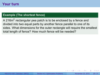
  • 55. Your turn Example (The shortest fence) A 216m2 rectangular pea patch is to be enclosed by a fence and divided into two equal parts by another fence parallel to one of its sides. What dimensions for the outer rectangle will require the smallest total length of fence? How much fence will be needed? . . . . . . V63.0121.021, Calculus I (NYU) Section 4.5 Optimization Problems November 23, 2010 25 / 31
  • 56. Your turn Example (The shortest fence) A 216m2 rectangular pea patch is to be enclosed by a fence and divided into two equal parts by another fence parallel to one of its sides. What dimensions for the outer rectangle will require the smallest total length of fence? How much fence will be needed? Solution Let the length and width of the pea patch be ℓ and w. The amount of fence needed is f = 2ℓ + 3w. Since ℓw = A, a constant, we have A f(w) = 2 + 3w. w The domain is all positive numbers. . . . . . . V63.0121.021, Calculus I (NYU) Section 4.5 Optimization Problems November 23, 2010 25 / 31
  • 57. Diagram w . ℓ f = 2ℓ + 3w A = ℓw ≡ 216 . . . . . . V63.0121.021, Calculus I (NYU) Section 4.5 Optimization Problems November 23, 2010 26 / 31
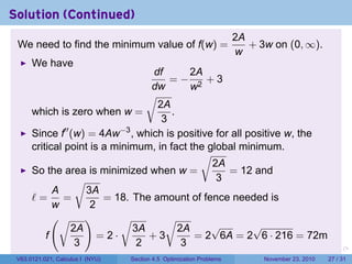
  • 58. Solution (Continued) 2A We need to find the minimum value of f(w) = + 3w on (0, ∞). w . . . . . . V63.0121.021, Calculus I (NYU) Section 4.5 Optimization Problems November 23, 2010 27 / 31
  • 59. Solution (Continued) 2A We need to find the minimum value of f(w) = + 3w on (0, ∞). w We have df 2A =− 2 +3 dw w √ 2A which is zero when w = . 3 . . . . . . V63.0121.021, Calculus I (NYU) Section 4.5 Optimization Problems November 23, 2010 27 / 31
  • 60. Solution (Continued) 2A We need to find the minimum value of f(w) = + 3w on (0, ∞). w We have df 2A =− 2 +3 dw w √ 2A which is zero when w = . 3 Since f′′ (w) = 4Aw−3 , which is positive for all positive w, the critical point is a minimum, in fact the global minimum. . . . . . . V63.0121.021, Calculus I (NYU) Section 4.5 Optimization Problems November 23, 2010 27 / 31
  • 61. Solution (Continued) 2A We need to find the minimum value of f(w) = + 3w on (0, ∞). w We have df 2A =− 2 +3 dw w √ 2A which is zero when w = . 3 Since f′′ (w) = 4Aw−3 , which is positive for all positive w, the critical point is a minimum, in fact the global minimum. √ 2A So the area is minimized when w = = 12 and √ 3 A 3A ℓ= = = 18. The amount of fence needed is w 2 (√ ) √ √ 2A 3A 2A √ √ f =2· +3 = 2 6A = 2 6 · 216 = 72m 3 2 3 . . . . . . V63.0121.021, Calculus I (NYU) Section 4.5 Optimization Problems November 23, 2010 27 / 31
  • 62. Try this one Example An advertisement consists of a rectangular printed region plus 1 in margins on the sides and 1.5 in margins on the top and bottom. If the total area of the advertisement is to be 120 in2 , what dimensions should the advertisement be to maximize the area of the printed region? . . . . . . V63.0121.021, Calculus I (NYU) Section 4.5 Optimization Problems November 23, 2010 28 / 31
  • 63. Try this one Example An advertisement consists of a rectangular printed region plus 1 in margins on the sides and 1.5 in margins on the top and bottom. If the total area of the advertisement is to be 120 in2 , what dimensions should the advertisement be to maximize the area of the printed region? Answer √ √ The optimal paper dimensions are 4 5 in by 6 5 in. . . . . . . V63.0121.021, Calculus I (NYU) Section 4.5 Optimization Problems November 23, 2010 28 / 31
  • 64. Solution Let the dimensions of the printed region be x and y, P 1.5 cm the printed area, and A the Lorem ipsum dolor sit amet, consectetur adipiscing elit. Nam paper area. We wish to dapibus vehicula mollis. Proin nec tristique mi. Pellentesque quis maximize P = xy subject to placerat dolor. Praesent a nisl diam. the constraint that Phasellus ut elit eu ligula accumsan euismod. Nunc condimentum lacinia risus a sodales. Morbi nunc risus, tincidunt in tristique sit amet, A = (x + 2)(y + 3) ≡ 120 1 cm 1 cm y ultrices eu eros. Proin pellentesque aliquam nibh ut lobortis. Ut et sollicitudin ipsum. Proin gravida Isolating y in A ≡ 120 gives ligula eget odio molestie rhoncus sed nec massa. In ante lorem, 120 imperdiet eget tincidunt at, pharetra y= − 3 which yields sit amet felis. Nunc nisi velit, x+2 tempus ac suscipit quis, blandit vitae mauris. Vestibulum ante ipsum ( ) primis in faucibus orci luctus et 120 120x . ultrices posuere cubilia Curae; P=x −3 = −3x x+2 x+2 1.5 cm The domain of P is (0, ∞). x . . . . . . V63.0121.021, Calculus I (NYU) Section 4.5 Optimization Problems November 23, 2010 29 / 31
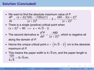
  • 65. Solution (Concluded) We want to find the absolute maximum value of P. dP (x + 2)(120) − (120x)(1) 240 − 3(x + 2)2 = −3= dx (x + 2)2 (x + 2)2 There is a single (positive) critical point when √ (x + 2)2 = 80 =⇒ x = 4 5 − 2. d2 P −480 The second derivative is 2 = , which is negative all dx (x + 2)3 along the domain of P. ( √ ) Hence the unique critical point x = 4 5 − 2 cm is the absolute maximum of P. √ This means the paper width is 4 5 cm, and the paper length is 120 √ √ = 6 5 cm. 4 5 . . . . . . V63.0121.021, Calculus I (NYU) Section 4.5 Optimization Problems November 23, 2010 30 / 31
  • 66. Summary Name [_ Problem Solving Strategy Draw a Picture Kathy had a box of 8 crayons. She gave some crayons away. She has 5 left. How many crayons did Kathy give away? Remember the checklist UNDERSTAND What do you want to find out? • Draw a line under the question. Ask yourself: what is the objective? You can draw a picture to solve the problem. Remember your geometry: What number do I add to 5 to get 8? 8 - = 5 similar triangles crayons 5 + 3 = 8 right triangles CHECK Does your answer make sense? trigonometric functions Explain. What number Draw a picture to solve the problem. do I add to 3 Write how many were given away. to make 10? I. I had 10 pencils. ft ft ft A I gave some away. 13 ill i :i I '•' I I I have 3 left. How many i? « 11 I pencils did I give away? I H 11 M i l ~7 U U U U> U U . . . . . . V63.0121.021, Calculus I (NYU) Section 4.5 Optimization Problems November 23, 2010 31 / 31