Lesson 18: Maximum and Minimum Values (Section 041 slides)
0 likes347 views

The document is a lecture note for a Calculus I course at New York University, focusing on maximum and minimum values, including concepts such as the extreme value theorem and Fermat's theorem. It outlines methods for finding extreme values of functions on closed intervals and discusses the significance of these values in optimization. The document also provides examples of continuous functions, illustrating cases where extreme values are achieved or not.


![The Extreme Value Theorem
Theorem (The Extreme Value Theorem)
Let f be a function which is continuous on the closed interval [a, b].
Then f attains an absolute maximum value f(c) and an absolute
minimum value f(d) at numbers c and d in [a, b].
V63.0121.041, Calculus I (NYU) Section 4.1 Maximum and Minimum Values November 8, 2010 13 / 34](https://image.slidesharecdn.com/lesson18-maximumandminimumvalues041slides-101108142857-phpapp02-121002220407-phpapp02/85/Lesson-18-Maximum-and-Minimum-Values-Section-041-slides-16-320.jpg)
![The Extreme Value Theorem
Theorem (The Extreme Value Theorem)
Let f be a function which is continuous on the closed interval [a, b].
Then f attains an absolute maximum value f(c) and an absolute
minimum value f(d) at numbers c and d in [a, b].
.
.
. .
a
. b
.
V63.0121.041, Calculus I (NYU) Section 4.1 Maximum and Minimum Values November 8, 2010 13 / 34](https://image.slidesharecdn.com/lesson18-maximumandminimumvalues041slides-101108142857-phpapp02-121002220407-phpapp02/85/Lesson-18-Maximum-and-Minimum-Values-Section-041-slides-17-320.jpg)
![The Extreme Value Theorem
Theorem (The Extreme Value Theorem)
Let f be a function which is continuous on the closed interval [a, b].
Then f attains an absolute maximum value f(c) and an absolute
minimum value f(d) at numbers c and d in [a, b].
.
maximum .(c)
f
.
value
. .
minimum .(d)
f
.
value
. . ..
a
. d c
b
.
minimum maximum
V63.0121.041, Calculus I (NYU) Section 4.1 Maximum and Minimum Values November 8, 2010 13 / 34](https://image.slidesharecdn.com/lesson18-maximumandminimumvalues041slides-101108142857-phpapp02-121002220407-phpapp02/85/Lesson-18-Maximum-and-Minimum-Values-Section-041-slides-18-320.jpg)
![Bad Example #1
Example
Consider the function .
{
x 0≤x<1
f(x) = . .
| .
x − 2 1 ≤ x ≤ 2. 1
.
.
Then although values of f(x) get arbitrarily close to 1 and never bigger
than 1, 1 is not the maximum value of f on [0, 1] because it is never
achieved.
V63.0121.041, Calculus I (NYU) Section 4.1 Maximum and Minimum Values November 8, 2010 15 / 34](https://image.slidesharecdn.com/lesson18-maximumandminimumvalues041slides-101108142857-phpapp02-121002220407-phpapp02/85/Lesson-18-Maximum-and-Minimum-Values-Section-041-slides-22-320.jpg)
![Bad Example #1
Example
Consider the function .
{
x 0≤x<1
f(x) = . .
| .
x − 2 1 ≤ x ≤ 2. 1
.
.
Then although values of f(x) get arbitrarily close to 1 and never bigger
than 1, 1 is not the maximum value of f on [0, 1] because it is never
achieved. This does not violate EVT because f is not continuous.
V63.0121.041, Calculus I (NYU) Section 4.1 Maximum and Minimum Values November 8, 2010 15 / 34](https://image.slidesharecdn.com/lesson18-maximumandminimumvalues041slides-101108142857-phpapp02-121002220407-phpapp02/85/Lesson-18-Maximum-and-Minimum-Values-Section-041-slides-23-320.jpg)


![Flowchart for placing extrema
Thanks to Fermat
Suppose f is a continuous function on the closed, bounded interval
[a, b], and c is a global maximum point.
.
. . c is a
start
local max
. . .
Is c an Is f diff’ble f is not
n
.o n
.o
endpoint? at c? diff at c
y
. es y
. es
. .
c = a or
f′ (c) = 0
c = b
V63.0121.041, Calculus I (NYU) Section 4.1 Maximum and Minimum Values November 8, 2010 26 / 34](https://image.slidesharecdn.com/lesson18-maximumandminimumvalues041slides-101108142857-phpapp02-121002220407-phpapp02/85/Lesson-18-Maximum-and-Minimum-Values-Section-041-slides-50-320.jpg)
![The Closed Interval Method
This means to find the maximum value of f on [a, b], we need to:
Evaluate f at the endpoints a and b
Evaluate f at the critical points or critical numbers x where
either f′ (x) = 0 or f is not differentiable at x.
The points with the largest function value are the global maximum
points
The points with the smallest or most negative function value are
the global minimum points.
V63.0121.041, Calculus I (NYU) Section 4.1 Maximum and Minimum Values November 8, 2010 27 / 34](https://image.slidesharecdn.com/lesson18-maximumandminimumvalues041slides-101108142857-phpapp02-121002220407-phpapp02/85/Lesson-18-Maximum-and-Minimum-Values-Section-041-slides-51-320.jpg)

![Extreme values of a linear function
Example
Find the extreme values of f(x) = 2x − 5 on [−1, 2].
V63.0121.041, Calculus I (NYU) Section 4.1 Maximum and Minimum Values November 8, 2010 29 / 34](https://image.slidesharecdn.com/lesson18-maximumandminimumvalues041slides-101108142857-phpapp02-121002220407-phpapp02/85/Lesson-18-Maximum-and-Minimum-Values-Section-041-slides-53-320.jpg)
![Extreme values of a linear function
Example
Find the extreme values of f(x) = 2x − 5 on [−1, 2].
Solution
Since f′ (x) = 2, which is never zero, we have no critical points and we
need only investigate the endpoints:
f(−1) = 2(−1) − 5 = −7
f(2) = 2(2) − 5 = −1
V63.0121.041, Calculus I (NYU) Section 4.1 Maximum and Minimum Values November 8, 2010 29 / 34](https://image.slidesharecdn.com/lesson18-maximumandminimumvalues041slides-101108142857-phpapp02-121002220407-phpapp02/85/Lesson-18-Maximum-and-Minimum-Values-Section-041-slides-54-320.jpg)
![Extreme values of a linear function
Example
Find the extreme values of f(x) = 2x − 5 on [−1, 2].
Solution
Since f′ (x) = 2, which is never zero, we have no critical points and we
need only investigate the endpoints:
f(−1) = 2(−1) − 5 = −7
f(2) = 2(2) − 5 = −1
So
The absolute minimum (point) is at −1; the minimum value is −7.
The absolute maximum (point) is at 2; the maximum value is −1.
V63.0121.041, Calculus I (NYU) Section 4.1 Maximum and Minimum Values November 8, 2010 29 / 34](https://image.slidesharecdn.com/lesson18-maximumandminimumvalues041slides-101108142857-phpapp02-121002220407-phpapp02/85/Lesson-18-Maximum-and-Minimum-Values-Section-041-slides-55-320.jpg)
![Extreme values of a quadratic function
Example
Find the extreme values of f(x) = x2 − 1 on [−1, 2].
V63.0121.041, Calculus I (NYU) Section 4.1 Maximum and Minimum Values November 8, 2010 30 / 34](https://image.slidesharecdn.com/lesson18-maximumandminimumvalues041slides-101108142857-phpapp02-121002220407-phpapp02/85/Lesson-18-Maximum-and-Minimum-Values-Section-041-slides-56-320.jpg)
![Extreme values of a quadratic function
Example
Find the extreme values of f(x) = x2 − 1 on [−1, 2].
Solution
We have f′ (x) = 2x, which is zero when x = 0.
V63.0121.041, Calculus I (NYU) Section 4.1 Maximum and Minimum Values November 8, 2010 30 / 34](https://image.slidesharecdn.com/lesson18-maximumandminimumvalues041slides-101108142857-phpapp02-121002220407-phpapp02/85/Lesson-18-Maximum-and-Minimum-Values-Section-041-slides-57-320.jpg)
![Extreme values of a quadratic function
Example
Find the extreme values of f(x) = x2 − 1 on [−1, 2].
Solution
We have f′ (x) = 2x, which is zero when x = 0. So our points to check
are:
f(−1) =
f(0) =
f(2) =
V63.0121.041, Calculus I (NYU) Section 4.1 Maximum and Minimum Values November 8, 2010 30 / 34](https://image.slidesharecdn.com/lesson18-maximumandminimumvalues041slides-101108142857-phpapp02-121002220407-phpapp02/85/Lesson-18-Maximum-and-Minimum-Values-Section-041-slides-58-320.jpg)
![Extreme values of a quadratic function
Example
Find the extreme values of f(x) = x2 − 1 on [−1, 2].
Solution
We have f′ (x) = 2x, which is zero when x = 0. So our points to check
are:
f(−1) = 0
f(0) =
f(2) =
V63.0121.041, Calculus I (NYU) Section 4.1 Maximum and Minimum Values November 8, 2010 30 / 34](https://image.slidesharecdn.com/lesson18-maximumandminimumvalues041slides-101108142857-phpapp02-121002220407-phpapp02/85/Lesson-18-Maximum-and-Minimum-Values-Section-041-slides-59-320.jpg)
![Extreme values of a quadratic function
Example
Find the extreme values of f(x) = x2 − 1 on [−1, 2].
Solution
We have f′ (x) = 2x, which is zero when x = 0. So our points to check
are:
f(−1) = 0
f(0) = − 1
f(2) =
V63.0121.041, Calculus I (NYU) Section 4.1 Maximum and Minimum Values November 8, 2010 30 / 34](https://image.slidesharecdn.com/lesson18-maximumandminimumvalues041slides-101108142857-phpapp02-121002220407-phpapp02/85/Lesson-18-Maximum-and-Minimum-Values-Section-041-slides-60-320.jpg)
![Extreme values of a quadratic function
Example
Find the extreme values of f(x) = x2 − 1 on [−1, 2].
Solution
We have f′ (x) = 2x, which is zero when x = 0. So our points to check
are:
f(−1) = 0
f(0) = − 1
f(2) = 3
V63.0121.041, Calculus I (NYU) Section 4.1 Maximum and Minimum Values November 8, 2010 30 / 34](https://image.slidesharecdn.com/lesson18-maximumandminimumvalues041slides-101108142857-phpapp02-121002220407-phpapp02/85/Lesson-18-Maximum-and-Minimum-Values-Section-041-slides-61-320.jpg)
![Extreme values of a quadratic function
Example
Find the extreme values of f(x) = x2 − 1 on [−1, 2].
Solution
We have f′ (x) = 2x, which is zero when x = 0. So our points to check
are:
f(−1) = 0
f(0) = − 1 (absolute min)
f(2) = 3
V63.0121.041, Calculus I (NYU) Section 4.1 Maximum and Minimum Values November 8, 2010 30 / 34](https://image.slidesharecdn.com/lesson18-maximumandminimumvalues041slides-101108142857-phpapp02-121002220407-phpapp02/85/Lesson-18-Maximum-and-Minimum-Values-Section-041-slides-62-320.jpg)
![Extreme values of a quadratic function
Example
Find the extreme values of f(x) = x2 − 1 on [−1, 2].
Solution
We have f′ (x) = 2x, which is zero when x = 0. So our points to check
are:
f(−1) = 0
f(0) = − 1 (absolute min)
f(2) = 3 (absolute max)
V63.0121.041, Calculus I (NYU) Section 4.1 Maximum and Minimum Values November 8, 2010 30 / 34](https://image.slidesharecdn.com/lesson18-maximumandminimumvalues041slides-101108142857-phpapp02-121002220407-phpapp02/85/Lesson-18-Maximum-and-Minimum-Values-Section-041-slides-63-320.jpg)
![Extreme values of a cubic function
Example
Find the extreme values of f(x) = 2x3 − 3x2 + 1 on [−1, 2].
V63.0121.041, Calculus I (NYU) Section 4.1 Maximum and Minimum Values November 8, 2010 31 / 34](https://image.slidesharecdn.com/lesson18-maximumandminimumvalues041slides-101108142857-phpapp02-121002220407-phpapp02/85/Lesson-18-Maximum-and-Minimum-Values-Section-041-slides-64-320.jpg)
![Extreme values of a cubic function
Example
Find the extreme values of f(x) = 2x3 − 3x2 + 1 on [−1, 2].
Solution
Since f′ (x) = 6x2 − 6x = 6x(x − 1), we have critical points at x = 0 and
x = 1.
V63.0121.041, Calculus I (NYU) Section 4.1 Maximum and Minimum Values November 8, 2010 31 / 34](https://image.slidesharecdn.com/lesson18-maximumandminimumvalues041slides-101108142857-phpapp02-121002220407-phpapp02/85/Lesson-18-Maximum-and-Minimum-Values-Section-041-slides-65-320.jpg)
![Extreme values of a cubic function
Example
Find the extreme values of f(x) = 2x3 − 3x2 + 1 on [−1, 2].
Solution
Since f′ (x) = 6x2 − 6x = 6x(x − 1), we have critical points at x = 0 and
x = 1. The values to check are
V63.0121.041, Calculus I (NYU) Section 4.1 Maximum and Minimum Values November 8, 2010 31 / 34](https://image.slidesharecdn.com/lesson18-maximumandminimumvalues041slides-101108142857-phpapp02-121002220407-phpapp02/85/Lesson-18-Maximum-and-Minimum-Values-Section-041-slides-66-320.jpg)
![Extreme values of a cubic function
Example
Find the extreme values of f(x) = 2x3 − 3x2 + 1 on [−1, 2].
Solution
Since f′ (x) = 6x2 − 6x = 6x(x − 1), we have critical points at x = 0 and
x = 1. The values to check are
f(−1) = − 4
V63.0121.041, Calculus I (NYU) Section 4.1 Maximum and Minimum Values November 8, 2010 31 / 34](https://image.slidesharecdn.com/lesson18-maximumandminimumvalues041slides-101108142857-phpapp02-121002220407-phpapp02/85/Lesson-18-Maximum-and-Minimum-Values-Section-041-slides-67-320.jpg)
![Extreme values of a cubic function
Example
Find the extreme values of f(x) = 2x3 − 3x2 + 1 on [−1, 2].
Solution
Since f′ (x) = 6x2 − 6x = 6x(x − 1), we have critical points at x = 0 and
x = 1. The values to check are
f(−1) = − 4
f(0) = 1
V63.0121.041, Calculus I (NYU) Section 4.1 Maximum and Minimum Values November 8, 2010 31 / 34](https://image.slidesharecdn.com/lesson18-maximumandminimumvalues041slides-101108142857-phpapp02-121002220407-phpapp02/85/Lesson-18-Maximum-and-Minimum-Values-Section-041-slides-68-320.jpg)
![Extreme values of a cubic function
Example
Find the extreme values of f(x) = 2x3 − 3x2 + 1 on [−1, 2].
Solution
Since f′ (x) = 6x2 − 6x = 6x(x − 1), we have critical points at x = 0 and
x = 1. The values to check are
f(−1) = − 4
f(0) = 1
f(1) = 0
V63.0121.041, Calculus I (NYU) Section 4.1 Maximum and Minimum Values November 8, 2010 31 / 34](https://image.slidesharecdn.com/lesson18-maximumandminimumvalues041slides-101108142857-phpapp02-121002220407-phpapp02/85/Lesson-18-Maximum-and-Minimum-Values-Section-041-slides-69-320.jpg)
![Extreme values of a cubic function
Example
Find the extreme values of f(x) = 2x3 − 3x2 + 1 on [−1, 2].
Solution
Since f′ (x) = 6x2 − 6x = 6x(x − 1), we have critical points at x = 0 and
x = 1. The values to check are
f(−1) = − 4
f(0) = 1
f(1) = 0
f(2) = 5
V63.0121.041, Calculus I (NYU) Section 4.1 Maximum and Minimum Values November 8, 2010 31 / 34](https://image.slidesharecdn.com/lesson18-maximumandminimumvalues041slides-101108142857-phpapp02-121002220407-phpapp02/85/Lesson-18-Maximum-and-Minimum-Values-Section-041-slides-70-320.jpg)
![Extreme values of a cubic function
Example
Find the extreme values of f(x) = 2x3 − 3x2 + 1 on [−1, 2].
Solution
Since f′ (x) = 6x2 − 6x = 6x(x − 1), we have critical points at x = 0 and
x = 1. The values to check are
f(−1) = − 4 (global min)
f(0) = 1
f(1) = 0
f(2) = 5
V63.0121.041, Calculus I (NYU) Section 4.1 Maximum and Minimum Values November 8, 2010 31 / 34](https://image.slidesharecdn.com/lesson18-maximumandminimumvalues041slides-101108142857-phpapp02-121002220407-phpapp02/85/Lesson-18-Maximum-and-Minimum-Values-Section-041-slides-71-320.jpg)
![Extreme values of a cubic function
Example
Find the extreme values of f(x) = 2x3 − 3x2 + 1 on [−1, 2].
Solution
Since f′ (x) = 6x2 − 6x = 6x(x − 1), we have critical points at x = 0 and
x = 1. The values to check are
f(−1) = − 4 (global min)
f(0) = 1
f(1) = 0
f(2) = 5 (global max)
V63.0121.041, Calculus I (NYU) Section 4.1 Maximum and Minimum Values November 8, 2010 31 / 34](https://image.slidesharecdn.com/lesson18-maximumandminimumvalues041slides-101108142857-phpapp02-121002220407-phpapp02/85/Lesson-18-Maximum-and-Minimum-Values-Section-041-slides-72-320.jpg)
![Extreme values of a cubic function
Example
Find the extreme values of f(x) = 2x3 − 3x2 + 1 on [−1, 2].
Solution
Since f′ (x) = 6x2 − 6x = 6x(x − 1), we have critical points at x = 0 and
x = 1. The values to check are
f(−1) = − 4 (global min)
f(0) = 1 (local max)
f(1) = 0
f(2) = 5 (global max)
V63.0121.041, Calculus I (NYU) Section 4.1 Maximum and Minimum Values November 8, 2010 31 / 34](https://image.slidesharecdn.com/lesson18-maximumandminimumvalues041slides-101108142857-phpapp02-121002220407-phpapp02/85/Lesson-18-Maximum-and-Minimum-Values-Section-041-slides-73-320.jpg)
![Extreme values of a cubic function
Example
Find the extreme values of f(x) = 2x3 − 3x2 + 1 on [−1, 2].
Solution
Since f′ (x) = 6x2 − 6x = 6x(x − 1), we have critical points at x = 0 and
x = 1. The values to check are
f(−1) = − 4 (global min)
f(0) = 1 (local max)
f(1) = 0 (local min)
f(2) = 5 (global max)
V63.0121.041, Calculus I (NYU) Section 4.1 Maximum and Minimum Values November 8, 2010 31 / 34](https://image.slidesharecdn.com/lesson18-maximumandminimumvalues041slides-101108142857-phpapp02-121002220407-phpapp02/85/Lesson-18-Maximum-and-Minimum-Values-Section-041-slides-74-320.jpg)
![Extreme values of an algebraic function
Example
Find the extreme values of f(x) = x2/3 (x + 2) on [−1, 2].
V63.0121.041, Calculus I (NYU) Section 4.1 Maximum and Minimum Values November 8, 2010 32 / 34](https://image.slidesharecdn.com/lesson18-maximumandminimumvalues041slides-101108142857-phpapp02-121002220407-phpapp02/85/Lesson-18-Maximum-and-Minimum-Values-Section-041-slides-75-320.jpg)
![Extreme values of an algebraic function
Example
Find the extreme values of f(x) = x2/3 (x + 2) on [−1, 2].
Solution
Write f(x) = x5/3 + 2x2/3 , then
5 2/3 4 −1/3 1 −1/3
f′ (x) = x + x = x (5x + 4)
3 3 3
Thus f′ (−4/5) = 0 and f is not differentiable at 0.
V63.0121.041, Calculus I (NYU) Section 4.1 Maximum and Minimum Values November 8, 2010 32 / 34](https://image.slidesharecdn.com/lesson18-maximumandminimumvalues041slides-101108142857-phpapp02-121002220407-phpapp02/85/Lesson-18-Maximum-and-Minimum-Values-Section-041-slides-76-320.jpg)
![Extreme values of an algebraic function
Example
Find the extreme values of f(x) = x2/3 (x + 2) on [−1, 2].
Solution
Write f(x) = x5/3 + 2x2/3 , then
5 2/3 4 −1/3 1 −1/3
f′ (x) = x + x = x (5x + 4)
3 3 3
Thus f′ (−4/5) = 0 and f is not differentiable at 0. So our points to
check are:
f(−1) =
V63.0121.041, Calculus I (NYU) Section 4.1 Maximum and Minimum Values November 8, 2010 32 / 34](https://image.slidesharecdn.com/lesson18-maximumandminimumvalues041slides-101108142857-phpapp02-121002220407-phpapp02/85/Lesson-18-Maximum-and-Minimum-Values-Section-041-slides-77-320.jpg)
![Extreme values of an algebraic function
Example
Find the extreme values of f(x) = x2/3 (x + 2) on [−1, 2].
Solution
Write f(x) = x5/3 + 2x2/3 , then
5 2/3 4 −1/3 1 −1/3
f′ (x) = x + x = x (5x + 4)
3 3 3
Thus f′ (−4/5) = 0 and f is not differentiable at 0. So our points to
check are:
f(−1) = 1
f(−4/5) =
V63.0121.041, Calculus I (NYU) Section 4.1 Maximum and Minimum Values November 8, 2010 32 / 34](https://image.slidesharecdn.com/lesson18-maximumandminimumvalues041slides-101108142857-phpapp02-121002220407-phpapp02/85/Lesson-18-Maximum-and-Minimum-Values-Section-041-slides-78-320.jpg)
![Extreme values of an algebraic function
Example
Find the extreme values of f(x) = x2/3 (x + 2) on [−1, 2].
Solution
Write f(x) = x5/3 + 2x2/3 , then
5 2/3 4 −1/3 1 −1/3
f′ (x) = x + x = x (5x + 4)
3 3 3
Thus f′ (−4/5) = 0 and f is not differentiable at 0. So our points to
check are:
f(−1) = 1
f(−4/5) = 1.0341
f(0) =
V63.0121.041, Calculus I (NYU) Section 4.1 Maximum and Minimum Values November 8, 2010 32 / 34](https://image.slidesharecdn.com/lesson18-maximumandminimumvalues041slides-101108142857-phpapp02-121002220407-phpapp02/85/Lesson-18-Maximum-and-Minimum-Values-Section-041-slides-79-320.jpg)
![Extreme values of an algebraic function
Example
Find the extreme values of f(x) = x2/3 (x + 2) on [−1, 2].
Solution
Write f(x) = x5/3 + 2x2/3 , then
5 2/3 4 −1/3 1 −1/3
f′ (x) = x + x = x (5x + 4)
3 3 3
Thus f′ (−4/5) = 0 and f is not differentiable at 0. So our points to
check are:
f(−1) = 1
f(−4/5) = 1.0341
f(0) = 0
f(2) =
V63.0121.041, Calculus I (NYU) Section 4.1 Maximum and Minimum Values November 8, 2010 32 / 34](https://image.slidesharecdn.com/lesson18-maximumandminimumvalues041slides-101108142857-phpapp02-121002220407-phpapp02/85/Lesson-18-Maximum-and-Minimum-Values-Section-041-slides-80-320.jpg)
![Extreme values of an algebraic function
Example
Find the extreme values of f(x) = x2/3 (x + 2) on [−1, 2].
Solution
Write f(x) = x5/3 + 2x2/3 , then
5 2/3 4 −1/3 1 −1/3
f′ (x) = x + x = x (5x + 4)
3 3 3
Thus f′ (−4/5) = 0 and f is not differentiable at 0. So our points to
check are:
f(−1) = 1
f(−4/5) = 1.0341
f(0) = 0
f(2) = 6.3496
V63.0121.041, Calculus I (NYU) Section 4.1 Maximum and Minimum Values November 8, 2010 32 / 34](https://image.slidesharecdn.com/lesson18-maximumandminimumvalues041slides-101108142857-phpapp02-121002220407-phpapp02/85/Lesson-18-Maximum-and-Minimum-Values-Section-041-slides-81-320.jpg)
![Extreme values of an algebraic function
Example
Find the extreme values of f(x) = x2/3 (x + 2) on [−1, 2].
Solution
Write f(x) = x5/3 + 2x2/3 , then
5 2/3 4 −1/3 1 −1/3
f′ (x) = x + x = x (5x + 4)
3 3 3
Thus f′ (−4/5) = 0 and f is not differentiable at 0. So our points to
check are:
f(−1) = 1
f(−4/5) = 1.0341
f(0) = 0 (absolute min)
f(2) = 6.3496
V63.0121.041, Calculus I (NYU) Section 4.1 Maximum and Minimum Values November 8, 2010 32 / 34](https://image.slidesharecdn.com/lesson18-maximumandminimumvalues041slides-101108142857-phpapp02-121002220407-phpapp02/85/Lesson-18-Maximum-and-Minimum-Values-Section-041-slides-82-320.jpg)
![Extreme values of an algebraic function
Example
Find the extreme values of f(x) = x2/3 (x + 2) on [−1, 2].
Solution
Write f(x) = x5/3 + 2x2/3 , then
5 2/3 4 −1/3 1 −1/3
f′ (x) = x + x = x (5x + 4)
3 3 3
Thus f′ (−4/5) = 0 and f is not differentiable at 0. So our points to
check are:
f(−1) = 1
f(−4/5) = 1.0341
f(0) = 0 (absolute min)
f(2) = 6.3496 (absolute max)
V63.0121.041, Calculus I (NYU) Section 4.1 Maximum and Minimum Values November 8, 2010 32 / 34](https://image.slidesharecdn.com/lesson18-maximumandminimumvalues041slides-101108142857-phpapp02-121002220407-phpapp02/85/Lesson-18-Maximum-and-Minimum-Values-Section-041-slides-83-320.jpg)
![Extreme values of an algebraic function
Example
Find the extreme values of f(x) = x2/3 (x + 2) on [−1, 2].
Solution
Write f(x) = x5/3 + 2x2/3 , then
5 2/3 4 −1/3 1 −1/3
f′ (x) = x + x = x (5x + 4)
3 3 3
Thus f′ (−4/5) = 0 and f is not differentiable at 0. So our points to
check are:
f(−1) = 1
f(−4/5) = 1.0341 (relative max)
f(0) = 0 (absolute min)
f(2) = 6.3496 (absolute max)
V63.0121.041, Calculus I (NYU) Section 4.1 Maximum and Minimum Values November 8, 2010 32 / 34](https://image.slidesharecdn.com/lesson18-maximumandminimumvalues041slides-101108142857-phpapp02-121002220407-phpapp02/85/Lesson-18-Maximum-and-Minimum-Values-Section-041-slides-84-320.jpg)
![Extreme values of another algebraic function
Example
√
Find the extreme values of f(x) = 4 − x2 on [−2, 1].
V63.0121.041, Calculus I (NYU) Section 4.1 Maximum and Minimum Values November 8, 2010 33 / 34](https://image.slidesharecdn.com/lesson18-maximumandminimumvalues041slides-101108142857-phpapp02-121002220407-phpapp02/85/Lesson-18-Maximum-and-Minimum-Values-Section-041-slides-85-320.jpg)
![Extreme values of another algebraic function
Example
√
Find the extreme values of f(x) = 4 − x2 on [−2, 1].
Solution
x
We have f′ (x) = − √ , which is zero when x = 0. (f is not
4 − x2
differentiable at ±2 as well.)
V63.0121.041, Calculus I (NYU) Section 4.1 Maximum and Minimum Values November 8, 2010 33 / 34](https://image.slidesharecdn.com/lesson18-maximumandminimumvalues041slides-101108142857-phpapp02-121002220407-phpapp02/85/Lesson-18-Maximum-and-Minimum-Values-Section-041-slides-86-320.jpg)
![Extreme values of another algebraic function
Example
√
Find the extreme values of f(x) = 4 − x2 on [−2, 1].
Solution
x
We have f′ (x) = − √ , which is zero when x = 0. (f is not
4 − x2
differentiable at ±2 as well.) So our points to check are:
f(−2) =
V63.0121.041, Calculus I (NYU) Section 4.1 Maximum and Minimum Values November 8, 2010 33 / 34](https://image.slidesharecdn.com/lesson18-maximumandminimumvalues041slides-101108142857-phpapp02-121002220407-phpapp02/85/Lesson-18-Maximum-and-Minimum-Values-Section-041-slides-87-320.jpg)
![Extreme values of another algebraic function
Example
√
Find the extreme values of f(x) = 4 − x2 on [−2, 1].
Solution
x
We have f′ (x) = − √ , which is zero when x = 0. (f is not
4 − x2
differentiable at ±2 as well.) So our points to check are:
f(−2) = 0
f(0) =
V63.0121.041, Calculus I (NYU) Section 4.1 Maximum and Minimum Values November 8, 2010 33 / 34](https://image.slidesharecdn.com/lesson18-maximumandminimumvalues041slides-101108142857-phpapp02-121002220407-phpapp02/85/Lesson-18-Maximum-and-Minimum-Values-Section-041-slides-88-320.jpg)
![Extreme values of another algebraic function
Example
√
Find the extreme values of f(x) = 4 − x2 on [−2, 1].
Solution
x
We have f′ (x) = − √ , which is zero when x = 0. (f is not
4 − x2
differentiable at ±2 as well.) So our points to check are:
f(−2) = 0
f(0) = 2
f(1) =
V63.0121.041, Calculus I (NYU) Section 4.1 Maximum and Minimum Values November 8, 2010 33 / 34](https://image.slidesharecdn.com/lesson18-maximumandminimumvalues041slides-101108142857-phpapp02-121002220407-phpapp02/85/Lesson-18-Maximum-and-Minimum-Values-Section-041-slides-89-320.jpg)
![Extreme values of another algebraic function
Example
√
Find the extreme values of f(x) = 4 − x2 on [−2, 1].
Solution
x
We have f′ (x) = − √ , which is zero when x = 0. (f is not
4 − x2
differentiable at ±2 as well.) So our points to check are:
f(−2) = 0
f(0) = 2
√
f(1) = 3
V63.0121.041, Calculus I (NYU) Section 4.1 Maximum and Minimum Values November 8, 2010 33 / 34](https://image.slidesharecdn.com/lesson18-maximumandminimumvalues041slides-101108142857-phpapp02-121002220407-phpapp02/85/Lesson-18-Maximum-and-Minimum-Values-Section-041-slides-90-320.jpg)
![Extreme values of another algebraic function
Example
√
Find the extreme values of f(x) = 4 − x2 on [−2, 1].
Solution
x
We have f′ (x) = − √ , which is zero when x = 0. (f is not
4 − x2
differentiable at ±2 as well.) So our points to check are:
f(−2) = 0 (absolute min)
f(0) = 2
√
f(1) = 3
V63.0121.041, Calculus I (NYU) Section 4.1 Maximum and Minimum Values November 8, 2010 33 / 34](https://image.slidesharecdn.com/lesson18-maximumandminimumvalues041slides-101108142857-phpapp02-121002220407-phpapp02/85/Lesson-18-Maximum-and-Minimum-Values-Section-041-slides-91-320.jpg)
![Extreme values of another algebraic function
Example
√
Find the extreme values of f(x) = 4 − x2 on [−2, 1].
Solution
x
We have f′ (x) = − √ , which is zero when x = 0. (f is not
4 − x2
differentiable at ±2 as well.) So our points to check are:
f(−2) = 0 (absolute min)
f(0) = 2 (absolute max)
√
f(1) = 3
V63.0121.041, Calculus I (NYU) Section 4.1 Maximum and Minimum Values November 8, 2010 33 / 34](https://image.slidesharecdn.com/lesson18-maximumandminimumvalues041slides-101108142857-phpapp02-121002220407-phpapp02/85/Lesson-18-Maximum-and-Minimum-Values-Section-041-slides-92-320.jpg)

Lesson 18: Maximum and Minimum Values (Section 041 slides)
- 1. Section 4.1 Maximum and Minimum Values V63.0121.041, Calculus I New York University November 8, 2010 Announcements Quiz 4 on Sections 3.3, 3.4, 3.5, and 3.7 next week (November 16, 18, or 19) . . . . . .
- 2. Announcements Quiz 4 on Sections 3.3, 3.4, 3.5, and 3.7 next week (November 16, 18, or 19) . . . . . . V63.0121.041, Calculus I (NYU) Section 4.1 Maximum and Minimum Values November 8, 2010 2 / 34
- 3. Objectives Understand and be able to explain the statement of the Extreme Value Theorem. Understand and be able to explain the statement of Fermat’s Theorem. Use the Closed Interval Method to find the extreme values of a function defined on a closed interval. . . . . . . V63.0121.041, Calculus I (NYU) Section 4.1 Maximum and Minimum Values November 8, 2010 3 / 34
- 4. Outline Introduction The Extreme Value Theorem Fermat’s Theorem (not the last one) Tangent: Fermat’s Last Theorem The Closed Interval Method Examples . . . . . . V63.0121.041, Calculus I (NYU) Section 4.1 Maximum and Minimum Values November 8, 2010 4 / 34
- 5. Optimize .
- 6. Why go to the extremes? Rationally speaking, it is advantageous to find the extreme values of a function (maximize profit, minimize costs, etc.) Pierre-Louis Maupertuis V63.0121.041, Calculus I (NYU) Section 4.1 Maximum and Minimum Values (1698–1759) 8, 2010 November 6 / 34
- 7. Design . Image credit: Jason Tromm . V63.0121.041, Calculus I (NYU) Section 4.1 Maximum and Minimum Values November 8, 2010 7 / 34
- 8. Why go to the extremes? Rationally speaking, it is advantageous to find the extreme values of a function (maximize profit, minimize costs, etc.) Many laws of science are derived from minimizing principles. Pierre-Louis Maupertuis V63.0121.041, Calculus I (NYU) Section 4.1 Maximum and Minimum Values (1698–1759) 8, 2010 November 8 / 34
- 9. Optics . Image credit: jacreative . V63.0121.041, Calculus I (NYU) Section 4.1 Maximum and Minimum Values November 8, 2010 9 / 34
- 10. Why go to the extremes? Rationally speaking, it is advantageous to find the extreme values of a function (maximize profit, minimize costs, etc.) Many laws of science are derived from minimizing principles. Maupertuis’ principle: “Action is minimized through the wisdom of God.” Pierre-Louis Maupertuis V63.0121.041, Calculus I (NYU) Section 4.1 Maximum and Minimum Values (1698–1759) 8, 2010 November 10 / 34
- 11. Outline Introduction The Extreme Value Theorem Fermat’s Theorem (not the last one) Tangent: Fermat’s Last Theorem The Closed Interval Method Examples V63.0121.041, Calculus I (NYU) Section 4.1 Maximum and Minimum Values November 8, 2010 11 / 34
- 12. Extreme points and values Definition Let f have domain D. . . Image credit: Patrick Q V63.0121.041, Calculus I (NYU) Section 4.1 Maximum and Minimum Values November 8, 2010 12 / 34
- 13. Extreme points and values Definition Let f have domain D. The function f has an absolute maximum (or global maximum) (respectively, absolute minimum) at c if f(c) ≥ f(x) (respectively, f(c) ≤ f(x)) for all x in D . . Image credit: Patrick Q V63.0121.041, Calculus I (NYU) Section 4.1 Maximum and Minimum Values November 8, 2010 12 / 34
- 14. Extreme points and values Definition Let f have domain D. The function f has an absolute maximum (or global maximum) (respectively, absolute minimum) at c if f(c) ≥ f(x) (respectively, f(c) ≤ f(x)) for all x in D The number f(c) is called the maximum value (respectively, minimum value) of f on D. . . Image credit: Patrick Q V63.0121.041, Calculus I (NYU) Section 4.1 Maximum and Minimum Values November 8, 2010 12 / 34
- 15. Extreme points and values Definition Let f have domain D. The function f has an absolute maximum (or global maximum) (respectively, absolute minimum) at c if f(c) ≥ f(x) (respectively, f(c) ≤ f(x)) for all x in D The number f(c) is called the maximum value (respectively, minimum value) of f on D. . An extremum is either a maximum or a minimum. An extreme value is either a .mage credit: Patrick Q value or minimum value. I maximum V63.0121.041, Calculus I (NYU) Section 4.1 Maximum and Minimum Values November 8, 2010 12 / 34
- 16. The Extreme Value Theorem Theorem (The Extreme Value Theorem) Let f be a function which is continuous on the closed interval [a, b]. Then f attains an absolute maximum value f(c) and an absolute minimum value f(d) at numbers c and d in [a, b]. V63.0121.041, Calculus I (NYU) Section 4.1 Maximum and Minimum Values November 8, 2010 13 / 34
- 17. The Extreme Value Theorem Theorem (The Extreme Value Theorem) Let f be a function which is continuous on the closed interval [a, b]. Then f attains an absolute maximum value f(c) and an absolute minimum value f(d) at numbers c and d in [a, b]. . . . . a . b . V63.0121.041, Calculus I (NYU) Section 4.1 Maximum and Minimum Values November 8, 2010 13 / 34
- 18. The Extreme Value Theorem Theorem (The Extreme Value Theorem) Let f be a function which is continuous on the closed interval [a, b]. Then f attains an absolute maximum value f(c) and an absolute minimum value f(d) at numbers c and d in [a, b]. . maximum .(c) f . value . . minimum .(d) f . value . . .. a . d c b . minimum maximum V63.0121.041, Calculus I (NYU) Section 4.1 Maximum and Minimum Values November 8, 2010 13 / 34
- 19. No proof of EVT forthcoming This theorem is very hard to prove without using technical facts about continuous functions and closed intervals. But we can show the importance of each of the hypotheses. V63.0121.041, Calculus I (NYU) Section 4.1 Maximum and Minimum Values November 8, 2010 14 / 34
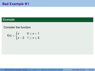
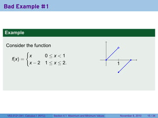
- 20. Bad Example #1 Example Consider the function { x 0≤x<1 f(x) = x − 2 1 ≤ x ≤ 2. V63.0121.041, Calculus I (NYU) Section 4.1 Maximum and Minimum Values November 8, 2010 15 / 34
- 21. Bad Example #1 Example Consider the function . { x 0≤x<1 f(x) = . . | . x − 2 1 ≤ x ≤ 2. 1 . . V63.0121.041, Calculus I (NYU) Section 4.1 Maximum and Minimum Values November 8, 2010 15 / 34
- 22. Bad Example #1 Example Consider the function . { x 0≤x<1 f(x) = . . | . x − 2 1 ≤ x ≤ 2. 1 . . Then although values of f(x) get arbitrarily close to 1 and never bigger than 1, 1 is not the maximum value of f on [0, 1] because it is never achieved. V63.0121.041, Calculus I (NYU) Section 4.1 Maximum and Minimum Values November 8, 2010 15 / 34
- 23. Bad Example #1 Example Consider the function . { x 0≤x<1 f(x) = . . | . x − 2 1 ≤ x ≤ 2. 1 . . Then although values of f(x) get arbitrarily close to 1 and never bigger than 1, 1 is not the maximum value of f on [0, 1] because it is never achieved. This does not violate EVT because f is not continuous. V63.0121.041, Calculus I (NYU) Section 4.1 Maximum and Minimum Values November 8, 2010 15 / 34
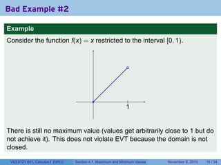
- 24. Bad Example #2 Example Consider the function f(x) = x restricted to the interval [0, 1). V63.0121.041, Calculus I (NYU) Section 4.1 Maximum and Minimum Values November 8, 2010 16 / 34
- 25. Bad Example #2 Example Consider the function f(x) = x restricted to the interval [0, 1). . . . | 1 . V63.0121.041, Calculus I (NYU) Section 4.1 Maximum and Minimum Values November 8, 2010 16 / 34
- 26. Bad Example #2 Example Consider the function f(x) = x restricted to the interval [0, 1). . . . | 1 . There is still no maximum value (values get arbitrarily close to 1 but do not achieve it). V63.0121.041, Calculus I (NYU) Section 4.1 Maximum and Minimum Values November 8, 2010 16 / 34
- 27. Bad Example #2 Example Consider the function f(x) = x restricted to the interval [0, 1). . . . | 1 . There is still no maximum value (values get arbitrarily close to 1 but do not achieve it). This does not violate EVT because the domain is not closed. V63.0121.041, Calculus I (NYU) Section 4.1 Maximum and Minimum Values November 8, 2010 16 / 34
- 28. Final Bad Example Example 1 Consider the function f(x) = is continuous on the closed interval x [1, ∞). V63.0121.041, Calculus I (NYU) Section 4.1 Maximum and Minimum Values November 8, 2010 17 / 34
- 29. Final Bad Example Example 1 Consider the function f(x) = is continuous on the closed interval x [1, ∞). . . . 1 . V63.0121.041, Calculus I (NYU) Section 4.1 Maximum and Minimum Values November 8, 2010 17 / 34
- 30. Final Bad Example Example 1 Consider the function f(x) = is continuous on the closed interval x [1, ∞). . . . 1 . There is no minimum value (values get arbitrarily close to 0 but do not achieve it). V63.0121.041, Calculus I (NYU) Section 4.1 Maximum and Minimum Values November 8, 2010 17 / 34
- 31. Final Bad Example Example 1 Consider the function f(x) = is continuous on the closed interval x [1, ∞). . . . 1 . There is no minimum value (values get arbitrarily close to 0 but do not achieve it). This does not violate EVT because the domain is not bounded. V63.0121.041, Calculus I (NYU) Section 4.1 Maximum and Minimum Values November 8, 2010 17 / 34
- 32. Outline Introduction The Extreme Value Theorem Fermat’s Theorem (not the last one) Tangent: Fermat’s Last Theorem The Closed Interval Method Examples V63.0121.041, Calculus I (NYU) Section 4.1 Maximum and Minimum Values November 8, 2010 18 / 34
- 33. Local extrema . Definition A function f has a local maximum or relative maximum at c if f(c) ≥ f(x) when x is near c. This means that f(c) ≥ f(x) for all x in some open interval containing c. Similarly, f has a local minimum at c if f(c) ≤ f(x) when x is near c. . V63.0121.041, Calculus I (NYU) Section 4.1 Maximum and Minimum Values November 8, 2010 19 / 34
- 34. Local extrema . Definition A function f has a local maximum or relative maximum at c if f(c) ≥ f(x) when x is near c. This means that f(c) ≥ f(x) for all x in some open interval containing c. Similarly, f has a local minimum at c if f(c) ≤ f(x) when x is near c. . . . . .|. . . . | a . local local b . maximum minimum . V63.0121.041, Calculus I (NYU) Section 4.1 Maximum and Minimum Values November 8, 2010 19 / 34
- 35. Local extrema . So a local extremum must be inside the domain of f (not on the end). A global extremum that is inside the domain is a local extremum. . . . . .|. . . .. | a . local local and global . global b maximum min max . V63.0121.041, Calculus I (NYU) Section 4.1 Maximum and Minimum Values November 8, 2010 19 / 34
- 36. Fermat's Theorem Theorem (Fermat’s Theorem) Suppose f has a local extremum at c and f is differentiable at c. Then f′ (c) = 0. . . . . ... | . . | a . local local b . maximum minimum V63.0121.041, Calculus I (NYU) Section 4.1 Maximum and Minimum Values November 8, 2010 21 / 34
- 37. Fermat's Theorem Theorem (Fermat’s Theorem) Suppose f has a local extremum at c and f is differentiable at c. Then f′ (c) = 0. . . . . ... | . . | a . local local b . maximum minimum V63.0121.041, Calculus I (NYU) Section 4.1 Maximum and Minimum Values November 8, 2010 21 / 34
- 38. Sketch of proof of Fermat's Theorem Suppose that f has a local maximum at c. V63.0121.041, Calculus I (NYU) Section 4.1 Maximum and Minimum Values November 8, 2010 22 / 34
- 39. Sketch of proof of Fermat's Theorem Suppose that f has a local maximum at c. If x is slightly greater than c, f(x) ≤ f(c). This means f(x) − f(c) ≤0 x−c V63.0121.041, Calculus I (NYU) Section 4.1 Maximum and Minimum Values November 8, 2010 22 / 34
- 40. Sketch of proof of Fermat's Theorem Suppose that f has a local maximum at c. If x is slightly greater than c, f(x) ≤ f(c). This means f(x) − f(c) f(x) − f(c) ≤ 0 =⇒ lim+ ≤0 x−c x→c x−c V63.0121.041, Calculus I (NYU) Section 4.1 Maximum and Minimum Values November 8, 2010 22 / 34
- 41. Sketch of proof of Fermat's Theorem Suppose that f has a local maximum at c. If x is slightly greater than c, f(x) ≤ f(c). This means f(x) − f(c) f(x) − f(c) ≤ 0 =⇒ lim+ ≤0 x−c x→c x−c The same will be true on the other end: if x is slightly less than c, f(x) ≤ f(c). This means f(x) − f(c) ≥0 x−c V63.0121.041, Calculus I (NYU) Section 4.1 Maximum and Minimum Values November 8, 2010 22 / 34
- 42. Sketch of proof of Fermat's Theorem Suppose that f has a local maximum at c. If x is slightly greater than c, f(x) ≤ f(c). This means f(x) − f(c) f(x) − f(c) ≤ 0 =⇒ lim+ ≤0 x−c x→c x−c The same will be true on the other end: if x is slightly less than c, f(x) ≤ f(c). This means f(x) − f(c) f(x) − f(c) ≥ 0 =⇒ lim ≥0 x−c x→c − x−c V63.0121.041, Calculus I (NYU) Section 4.1 Maximum and Minimum Values November 8, 2010 22 / 34
- 43. Sketch of proof of Fermat's Theorem Suppose that f has a local maximum at c. If x is slightly greater than c, f(x) ≤ f(c). This means f(x) − f(c) f(x) − f(c) ≤ 0 =⇒ lim+ ≤0 x−c x→c x−c The same will be true on the other end: if x is slightly less than c, f(x) ≤ f(c). This means f(x) − f(c) f(x) − f(c) ≥ 0 =⇒ lim ≥0 x−c x→c − x−c f(x) − f(c) Since the limit f′ (c) = lim exists, it must be 0. x→c x−c V63.0121.041, Calculus I (NYU) Section 4.1 Maximum and Minimum Values November 8, 2010 22 / 34
- 44. Meet the Mathematician: Pierre de Fermat 1601–1665 Lawyer and number theorist Proved many theorems, didn’t quite prove his last one V63.0121.041, Calculus I (NYU) Section 4.1 Maximum and Minimum Values November 8, 2010 23 / 34
- 45. Tangent: Fermat's Last Theorem Plenty of solutions to x2 + y2 = z2 among positive whole numbers (e.g., x = 3, y = 4, z = 5) V63.0121.041, Calculus I (NYU) Section 4.1 Maximum and Minimum Values November 8, 2010 24 / 34
- 46. Tangent: Fermat's Last Theorem Plenty of solutions to x2 + y2 = z2 among positive whole numbers (e.g., x = 3, y = 4, z = 5) No solutions to x3 + y3 = z3 among positive whole numbers V63.0121.041, Calculus I (NYU) Section 4.1 Maximum and Minimum Values November 8, 2010 24 / 34
- 47. Tangent: Fermat's Last Theorem Plenty of solutions to x2 + y2 = z2 among positive whole numbers (e.g., x = 3, y = 4, z = 5) No solutions to x3 + y3 = z3 among positive whole numbers Fermat claimed no solutions to xn + yn = zn but didn’t write down his proof V63.0121.041, Calculus I (NYU) Section 4.1 Maximum and Minimum Values November 8, 2010 24 / 34
- 48. Tangent: Fermat's Last Theorem Plenty of solutions to x2 + y2 = z2 among positive whole numbers (e.g., x = 3, y = 4, z = 5) No solutions to x3 + y3 = z3 among positive whole numbers Fermat claimed no solutions to xn + yn = zn but didn’t write down his proof Not solved until 1998! (Taylor–Wiles) V63.0121.041, Calculus I (NYU) Section 4.1 Maximum and Minimum Values November 8, 2010 24 / 34
- 49. Outline Introduction The Extreme Value Theorem Fermat’s Theorem (not the last one) Tangent: Fermat’s Last Theorem The Closed Interval Method Examples V63.0121.041, Calculus I (NYU) Section 4.1 Maximum and Minimum Values November 8, 2010 25 / 34
- 50. Flowchart for placing extrema Thanks to Fermat Suppose f is a continuous function on the closed, bounded interval [a, b], and c is a global maximum point. . . . c is a start local max . . . Is c an Is f diff’ble f is not n .o n .o endpoint? at c? diff at c y . es y . es . . c = a or f′ (c) = 0 c = b V63.0121.041, Calculus I (NYU) Section 4.1 Maximum and Minimum Values November 8, 2010 26 / 34
- 51. The Closed Interval Method This means to find the maximum value of f on [a, b], we need to: Evaluate f at the endpoints a and b Evaluate f at the critical points or critical numbers x where either f′ (x) = 0 or f is not differentiable at x. The points with the largest function value are the global maximum points The points with the smallest or most negative function value are the global minimum points. V63.0121.041, Calculus I (NYU) Section 4.1 Maximum and Minimum Values November 8, 2010 27 / 34
- 52. Outline Introduction The Extreme Value Theorem Fermat’s Theorem (not the last one) Tangent: Fermat’s Last Theorem The Closed Interval Method Examples V63.0121.041, Calculus I (NYU) Section 4.1 Maximum and Minimum Values November 8, 2010 28 / 34
- 53. Extreme values of a linear function Example Find the extreme values of f(x) = 2x − 5 on [−1, 2]. V63.0121.041, Calculus I (NYU) Section 4.1 Maximum and Minimum Values November 8, 2010 29 / 34
- 54. Extreme values of a linear function Example Find the extreme values of f(x) = 2x − 5 on [−1, 2]. Solution Since f′ (x) = 2, which is never zero, we have no critical points and we need only investigate the endpoints: f(−1) = 2(−1) − 5 = −7 f(2) = 2(2) − 5 = −1 V63.0121.041, Calculus I (NYU) Section 4.1 Maximum and Minimum Values November 8, 2010 29 / 34
- 55. Extreme values of a linear function Example Find the extreme values of f(x) = 2x − 5 on [−1, 2]. Solution Since f′ (x) = 2, which is never zero, we have no critical points and we need only investigate the endpoints: f(−1) = 2(−1) − 5 = −7 f(2) = 2(2) − 5 = −1 So The absolute minimum (point) is at −1; the minimum value is −7. The absolute maximum (point) is at 2; the maximum value is −1. V63.0121.041, Calculus I (NYU) Section 4.1 Maximum and Minimum Values November 8, 2010 29 / 34
- 56. Extreme values of a quadratic function Example Find the extreme values of f(x) = x2 − 1 on [−1, 2]. V63.0121.041, Calculus I (NYU) Section 4.1 Maximum and Minimum Values November 8, 2010 30 / 34
- 57. Extreme values of a quadratic function Example Find the extreme values of f(x) = x2 − 1 on [−1, 2]. Solution We have f′ (x) = 2x, which is zero when x = 0. V63.0121.041, Calculus I (NYU) Section 4.1 Maximum and Minimum Values November 8, 2010 30 / 34
- 58. Extreme values of a quadratic function Example Find the extreme values of f(x) = x2 − 1 on [−1, 2]. Solution We have f′ (x) = 2x, which is zero when x = 0. So our points to check are: f(−1) = f(0) = f(2) = V63.0121.041, Calculus I (NYU) Section 4.1 Maximum and Minimum Values November 8, 2010 30 / 34
- 59. Extreme values of a quadratic function Example Find the extreme values of f(x) = x2 − 1 on [−1, 2]. Solution We have f′ (x) = 2x, which is zero when x = 0. So our points to check are: f(−1) = 0 f(0) = f(2) = V63.0121.041, Calculus I (NYU) Section 4.1 Maximum and Minimum Values November 8, 2010 30 / 34
- 60. Extreme values of a quadratic function Example Find the extreme values of f(x) = x2 − 1 on [−1, 2]. Solution We have f′ (x) = 2x, which is zero when x = 0. So our points to check are: f(−1) = 0 f(0) = − 1 f(2) = V63.0121.041, Calculus I (NYU) Section 4.1 Maximum and Minimum Values November 8, 2010 30 / 34
- 61. Extreme values of a quadratic function Example Find the extreme values of f(x) = x2 − 1 on [−1, 2]. Solution We have f′ (x) = 2x, which is zero when x = 0. So our points to check are: f(−1) = 0 f(0) = − 1 f(2) = 3 V63.0121.041, Calculus I (NYU) Section 4.1 Maximum and Minimum Values November 8, 2010 30 / 34
- 62. Extreme values of a quadratic function Example Find the extreme values of f(x) = x2 − 1 on [−1, 2]. Solution We have f′ (x) = 2x, which is zero when x = 0. So our points to check are: f(−1) = 0 f(0) = − 1 (absolute min) f(2) = 3 V63.0121.041, Calculus I (NYU) Section 4.1 Maximum and Minimum Values November 8, 2010 30 / 34
- 63. Extreme values of a quadratic function Example Find the extreme values of f(x) = x2 − 1 on [−1, 2]. Solution We have f′ (x) = 2x, which is zero when x = 0. So our points to check are: f(−1) = 0 f(0) = − 1 (absolute min) f(2) = 3 (absolute max) V63.0121.041, Calculus I (NYU) Section 4.1 Maximum and Minimum Values November 8, 2010 30 / 34
- 64. Extreme values of a cubic function Example Find the extreme values of f(x) = 2x3 − 3x2 + 1 on [−1, 2]. V63.0121.041, Calculus I (NYU) Section 4.1 Maximum and Minimum Values November 8, 2010 31 / 34
- 65. Extreme values of a cubic function Example Find the extreme values of f(x) = 2x3 − 3x2 + 1 on [−1, 2]. Solution Since f′ (x) = 6x2 − 6x = 6x(x − 1), we have critical points at x = 0 and x = 1. V63.0121.041, Calculus I (NYU) Section 4.1 Maximum and Minimum Values November 8, 2010 31 / 34
- 66. Extreme values of a cubic function Example Find the extreme values of f(x) = 2x3 − 3x2 + 1 on [−1, 2]. Solution Since f′ (x) = 6x2 − 6x = 6x(x − 1), we have critical points at x = 0 and x = 1. The values to check are V63.0121.041, Calculus I (NYU) Section 4.1 Maximum and Minimum Values November 8, 2010 31 / 34
- 67. Extreme values of a cubic function Example Find the extreme values of f(x) = 2x3 − 3x2 + 1 on [−1, 2]. Solution Since f′ (x) = 6x2 − 6x = 6x(x − 1), we have critical points at x = 0 and x = 1. The values to check are f(−1) = − 4 V63.0121.041, Calculus I (NYU) Section 4.1 Maximum and Minimum Values November 8, 2010 31 / 34
- 68. Extreme values of a cubic function Example Find the extreme values of f(x) = 2x3 − 3x2 + 1 on [−1, 2]. Solution Since f′ (x) = 6x2 − 6x = 6x(x − 1), we have critical points at x = 0 and x = 1. The values to check are f(−1) = − 4 f(0) = 1 V63.0121.041, Calculus I (NYU) Section 4.1 Maximum and Minimum Values November 8, 2010 31 / 34
- 69. Extreme values of a cubic function Example Find the extreme values of f(x) = 2x3 − 3x2 + 1 on [−1, 2]. Solution Since f′ (x) = 6x2 − 6x = 6x(x − 1), we have critical points at x = 0 and x = 1. The values to check are f(−1) = − 4 f(0) = 1 f(1) = 0 V63.0121.041, Calculus I (NYU) Section 4.1 Maximum and Minimum Values November 8, 2010 31 / 34
- 70. Extreme values of a cubic function Example Find the extreme values of f(x) = 2x3 − 3x2 + 1 on [−1, 2]. Solution Since f′ (x) = 6x2 − 6x = 6x(x − 1), we have critical points at x = 0 and x = 1. The values to check are f(−1) = − 4 f(0) = 1 f(1) = 0 f(2) = 5 V63.0121.041, Calculus I (NYU) Section 4.1 Maximum and Minimum Values November 8, 2010 31 / 34
- 71. Extreme values of a cubic function Example Find the extreme values of f(x) = 2x3 − 3x2 + 1 on [−1, 2]. Solution Since f′ (x) = 6x2 − 6x = 6x(x − 1), we have critical points at x = 0 and x = 1. The values to check are f(−1) = − 4 (global min) f(0) = 1 f(1) = 0 f(2) = 5 V63.0121.041, Calculus I (NYU) Section 4.1 Maximum and Minimum Values November 8, 2010 31 / 34
- 72. Extreme values of a cubic function Example Find the extreme values of f(x) = 2x3 − 3x2 + 1 on [−1, 2]. Solution Since f′ (x) = 6x2 − 6x = 6x(x − 1), we have critical points at x = 0 and x = 1. The values to check are f(−1) = − 4 (global min) f(0) = 1 f(1) = 0 f(2) = 5 (global max) V63.0121.041, Calculus I (NYU) Section 4.1 Maximum and Minimum Values November 8, 2010 31 / 34
- 73. Extreme values of a cubic function Example Find the extreme values of f(x) = 2x3 − 3x2 + 1 on [−1, 2]. Solution Since f′ (x) = 6x2 − 6x = 6x(x − 1), we have critical points at x = 0 and x = 1. The values to check are f(−1) = − 4 (global min) f(0) = 1 (local max) f(1) = 0 f(2) = 5 (global max) V63.0121.041, Calculus I (NYU) Section 4.1 Maximum and Minimum Values November 8, 2010 31 / 34
- 74. Extreme values of a cubic function Example Find the extreme values of f(x) = 2x3 − 3x2 + 1 on [−1, 2]. Solution Since f′ (x) = 6x2 − 6x = 6x(x − 1), we have critical points at x = 0 and x = 1. The values to check are f(−1) = − 4 (global min) f(0) = 1 (local max) f(1) = 0 (local min) f(2) = 5 (global max) V63.0121.041, Calculus I (NYU) Section 4.1 Maximum and Minimum Values November 8, 2010 31 / 34
- 75. Extreme values of an algebraic function Example Find the extreme values of f(x) = x2/3 (x + 2) on [−1, 2]. V63.0121.041, Calculus I (NYU) Section 4.1 Maximum and Minimum Values November 8, 2010 32 / 34
- 76. Extreme values of an algebraic function Example Find the extreme values of f(x) = x2/3 (x + 2) on [−1, 2]. Solution Write f(x) = x5/3 + 2x2/3 , then 5 2/3 4 −1/3 1 −1/3 f′ (x) = x + x = x (5x + 4) 3 3 3 Thus f′ (−4/5) = 0 and f is not differentiable at 0. V63.0121.041, Calculus I (NYU) Section 4.1 Maximum and Minimum Values November 8, 2010 32 / 34
- 77. Extreme values of an algebraic function Example Find the extreme values of f(x) = x2/3 (x + 2) on [−1, 2]. Solution Write f(x) = x5/3 + 2x2/3 , then 5 2/3 4 −1/3 1 −1/3 f′ (x) = x + x = x (5x + 4) 3 3 3 Thus f′ (−4/5) = 0 and f is not differentiable at 0. So our points to check are: f(−1) = V63.0121.041, Calculus I (NYU) Section 4.1 Maximum and Minimum Values November 8, 2010 32 / 34
- 78. Extreme values of an algebraic function Example Find the extreme values of f(x) = x2/3 (x + 2) on [−1, 2]. Solution Write f(x) = x5/3 + 2x2/3 , then 5 2/3 4 −1/3 1 −1/3 f′ (x) = x + x = x (5x + 4) 3 3 3 Thus f′ (−4/5) = 0 and f is not differentiable at 0. So our points to check are: f(−1) = 1 f(−4/5) = V63.0121.041, Calculus I (NYU) Section 4.1 Maximum and Minimum Values November 8, 2010 32 / 34
- 79. Extreme values of an algebraic function Example Find the extreme values of f(x) = x2/3 (x + 2) on [−1, 2]. Solution Write f(x) = x5/3 + 2x2/3 , then 5 2/3 4 −1/3 1 −1/3 f′ (x) = x + x = x (5x + 4) 3 3 3 Thus f′ (−4/5) = 0 and f is not differentiable at 0. So our points to check are: f(−1) = 1 f(−4/5) = 1.0341 f(0) = V63.0121.041, Calculus I (NYU) Section 4.1 Maximum and Minimum Values November 8, 2010 32 / 34
- 80. Extreme values of an algebraic function Example Find the extreme values of f(x) = x2/3 (x + 2) on [−1, 2]. Solution Write f(x) = x5/3 + 2x2/3 , then 5 2/3 4 −1/3 1 −1/3 f′ (x) = x + x = x (5x + 4) 3 3 3 Thus f′ (−4/5) = 0 and f is not differentiable at 0. So our points to check are: f(−1) = 1 f(−4/5) = 1.0341 f(0) = 0 f(2) = V63.0121.041, Calculus I (NYU) Section 4.1 Maximum and Minimum Values November 8, 2010 32 / 34
- 81. Extreme values of an algebraic function Example Find the extreme values of f(x) = x2/3 (x + 2) on [−1, 2]. Solution Write f(x) = x5/3 + 2x2/3 , then 5 2/3 4 −1/3 1 −1/3 f′ (x) = x + x = x (5x + 4) 3 3 3 Thus f′ (−4/5) = 0 and f is not differentiable at 0. So our points to check are: f(−1) = 1 f(−4/5) = 1.0341 f(0) = 0 f(2) = 6.3496 V63.0121.041, Calculus I (NYU) Section 4.1 Maximum and Minimum Values November 8, 2010 32 / 34
- 82. Extreme values of an algebraic function Example Find the extreme values of f(x) = x2/3 (x + 2) on [−1, 2]. Solution Write f(x) = x5/3 + 2x2/3 , then 5 2/3 4 −1/3 1 −1/3 f′ (x) = x + x = x (5x + 4) 3 3 3 Thus f′ (−4/5) = 0 and f is not differentiable at 0. So our points to check are: f(−1) = 1 f(−4/5) = 1.0341 f(0) = 0 (absolute min) f(2) = 6.3496 V63.0121.041, Calculus I (NYU) Section 4.1 Maximum and Minimum Values November 8, 2010 32 / 34
- 83. Extreme values of an algebraic function Example Find the extreme values of f(x) = x2/3 (x + 2) on [−1, 2]. Solution Write f(x) = x5/3 + 2x2/3 , then 5 2/3 4 −1/3 1 −1/3 f′ (x) = x + x = x (5x + 4) 3 3 3 Thus f′ (−4/5) = 0 and f is not differentiable at 0. So our points to check are: f(−1) = 1 f(−4/5) = 1.0341 f(0) = 0 (absolute min) f(2) = 6.3496 (absolute max) V63.0121.041, Calculus I (NYU) Section 4.1 Maximum and Minimum Values November 8, 2010 32 / 34
- 84. Extreme values of an algebraic function Example Find the extreme values of f(x) = x2/3 (x + 2) on [−1, 2]. Solution Write f(x) = x5/3 + 2x2/3 , then 5 2/3 4 −1/3 1 −1/3 f′ (x) = x + x = x (5x + 4) 3 3 3 Thus f′ (−4/5) = 0 and f is not differentiable at 0. So our points to check are: f(−1) = 1 f(−4/5) = 1.0341 (relative max) f(0) = 0 (absolute min) f(2) = 6.3496 (absolute max) V63.0121.041, Calculus I (NYU) Section 4.1 Maximum and Minimum Values November 8, 2010 32 / 34
- 85. Extreme values of another algebraic function Example √ Find the extreme values of f(x) = 4 − x2 on [−2, 1]. V63.0121.041, Calculus I (NYU) Section 4.1 Maximum and Minimum Values November 8, 2010 33 / 34
- 86. Extreme values of another algebraic function Example √ Find the extreme values of f(x) = 4 − x2 on [−2, 1]. Solution x We have f′ (x) = − √ , which is zero when x = 0. (f is not 4 − x2 differentiable at ±2 as well.) V63.0121.041, Calculus I (NYU) Section 4.1 Maximum and Minimum Values November 8, 2010 33 / 34
- 87. Extreme values of another algebraic function Example √ Find the extreme values of f(x) = 4 − x2 on [−2, 1]. Solution x We have f′ (x) = − √ , which is zero when x = 0. (f is not 4 − x2 differentiable at ±2 as well.) So our points to check are: f(−2) = V63.0121.041, Calculus I (NYU) Section 4.1 Maximum and Minimum Values November 8, 2010 33 / 34
- 88. Extreme values of another algebraic function Example √ Find the extreme values of f(x) = 4 − x2 on [−2, 1]. Solution x We have f′ (x) = − √ , which is zero when x = 0. (f is not 4 − x2 differentiable at ±2 as well.) So our points to check are: f(−2) = 0 f(0) = V63.0121.041, Calculus I (NYU) Section 4.1 Maximum and Minimum Values November 8, 2010 33 / 34
- 89. Extreme values of another algebraic function Example √ Find the extreme values of f(x) = 4 − x2 on [−2, 1]. Solution x We have f′ (x) = − √ , which is zero when x = 0. (f is not 4 − x2 differentiable at ±2 as well.) So our points to check are: f(−2) = 0 f(0) = 2 f(1) = V63.0121.041, Calculus I (NYU) Section 4.1 Maximum and Minimum Values November 8, 2010 33 / 34
- 90. Extreme values of another algebraic function Example √ Find the extreme values of f(x) = 4 − x2 on [−2, 1]. Solution x We have f′ (x) = − √ , which is zero when x = 0. (f is not 4 − x2 differentiable at ±2 as well.) So our points to check are: f(−2) = 0 f(0) = 2 √ f(1) = 3 V63.0121.041, Calculus I (NYU) Section 4.1 Maximum and Minimum Values November 8, 2010 33 / 34
- 91. Extreme values of another algebraic function Example √ Find the extreme values of f(x) = 4 − x2 on [−2, 1]. Solution x We have f′ (x) = − √ , which is zero when x = 0. (f is not 4 − x2 differentiable at ±2 as well.) So our points to check are: f(−2) = 0 (absolute min) f(0) = 2 √ f(1) = 3 V63.0121.041, Calculus I (NYU) Section 4.1 Maximum and Minimum Values November 8, 2010 33 / 34
- 92. Extreme values of another algebraic function Example √ Find the extreme values of f(x) = 4 − x2 on [−2, 1]. Solution x We have f′ (x) = − √ , which is zero when x = 0. (f is not 4 − x2 differentiable at ±2 as well.) So our points to check are: f(−2) = 0 (absolute min) f(0) = 2 (absolute max) √ f(1) = 3 V63.0121.041, Calculus I (NYU) Section 4.1 Maximum and Minimum Values November 8, 2010 33 / 34
- 93. Summary The Extreme Value Theorem: a continuous function on a closed interval must achieve its max and min Fermat’s Theorem: local extrema are critical points The Closed Interval Method: an algorithm for finding global extrema Show your work unless you want to end up like Fermat! V63.0121.041, Calculus I (NYU) Section 4.1 Maximum and Minimum Values November 8, 2010 34 / 34