SlideShare a Scribd company logo
MapReduce Algorithm Design
MapReduce: Recap
• Programmers must specify:
map (k, v) → <k’, v’>*
reduce (k’, v’) → <k’, v’>*
– All values with the same key are reduced together
• Optionally, also:
partition (k’, number of partitions) → partition for k’
– Often a simple hash of the key, e.g., hash(k’) mod n
– Divides up key space for parallel reduce operations
combine (k’, v’) → <k’, v’>*
– Mini-reducers that run in memory after the map phase
– Used as an optimization to reduce network traffic
• The execution framework handles everything else…
“Everything Else”
• The execution framework handles everything else…
– Scheduling: assigns workers to map and reduce tasks
– “Data distribution”: moves processes to data
– Synchronization: gathers, sorts, and shuffles intermediate data
– Errors and faults: detects worker failures and restarts
• Limited control over data and execution flow
– All algorithms must expressed in m, r, c, p
• You don’t know:
– Where mappers and reducers run
– When a mapper or reducer begins or finishes
– Which input a particular mapper is processing
– Which intermediate key a particular reducer is processing
combine
combine combine combine
b
a 1 2 c 9 a c
5 2 b c
7 8
partition partition partition partition
map
map map map
k1 k2 k3 k4 k5 k6
v1 v2 v3 v4 v5 v6
b
a 1 2 c c
3 6 a c
5 2 b c
7 8
Shuffle and Sort: aggregate values by keys
reduce reduce reduce
a 1 5 b 2 7 c 2 9 8
r1 s1 r2 s2 r3 s3
Tools for Synchronization
• Cleverly-constructed data structures
– Bring partial results together
• Sort order of intermediate keys
– Control order in which reducers process keys
• Partitioner
– Control which reducer processes which keys
• Preserving state in mappers and reducers
– Capture dependencies across multiple keys and
values
Preserving State
Mapper object
configure
map
close
state
one object per task
Reducer object
configure
reduce
close
state
one call per input
key-value pair
one call per
intermediate key
API initialization hook
API cleanup hook
Scalable Hadoop Algorithms: Themes
• Avoid object creation
– Inherently costly operation
– Garbage collection
• Avoid buffering
– Limited heap size
– Works for small datasets, but won’t scale!
Importance of Local Aggregation
• Ideal scaling characteristics:
– Twice the data, twice the running time
– Twice the resources, half the running time
• Why can’t we achieve this?
– Synchronization requires communication
– Communication kills performance
• Thus… avoid communication!
– Reduce intermediate data via local aggregation
– Combiners can help
Shuffle and Sort
Mapper
Reducer
other mappers
other reducers
circular buffer
(in memory)
spills (on disk)
merged spills
(on disk)
intermediate files
(on disk)
Combiner
Combiner
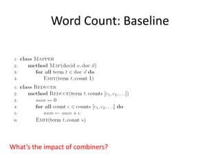
Word Count: Baseline
What’s the impact of combiners?
Word Count: Version 1
Are combiners still needed?
Word Count: Version 2
Are combiners still needed?
Design Pattern for Local Aggregation
• “In-mapper combining”
– Fold the functionality of the combiner into the
mapper by preserving state across multiple map calls
• Advantages
– Speed
– Why is this faster than actual combiners?
• Disadvantages
– Explicit memory management required
– Potential for order-dependent bugs
Combiner Design
• Combiners and reducers share same method
signature
– Sometimes, reducers can serve as combiners
– Often, not…
• Remember: combiner are optional optimizations
– Should not affect algorithm correctness
– May be run 0, 1, or multiple times
• Example: find average of all integers associated
with the same key
Computing the Mean: Version 1
Why can’t we use reducer as combiner?
Computing the Mean: Version 2
Why doesn’t this work?
Computing the Mean: Version 3
Fixed?
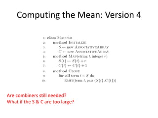
Computing the Mean: Version 4
Are combiners still needed?
What if the S & C are too large?
Algorithm Design: Running Example
• Term co-occurrence matrix for a text collection
– M = N x N matrix (N = vocabulary size)
– Mij: number of times i and j co-occur in some context
(for concreteness, let’s say context = sentence)
• Why?
– Distributional profiles as a way of measuring semantic
distance
– Semantic distance useful for many language
processing tasks
MapReduce: Large Counting Problems
• Term co-occurrence matrix for a text collection
= specific instance of a large counting problem
– A large event space (number of terms)
– A large number of observations (the collection itself)
– Goal: keep track of interesting statistics about the
events
• Basic approach
– Mappers generate partial counts
– Reducers aggregate partial counts
How do we aggregate partial counts efficiently?
First Try: “Pairs”
• Each mapper takes a sentence:
– Generate all co-occurring term pairs
– For all pairs, emit (a, b) → count
• Reducers sum up counts associated with these
pairs
• Use combiners!
Pairs: Pseudo-Code
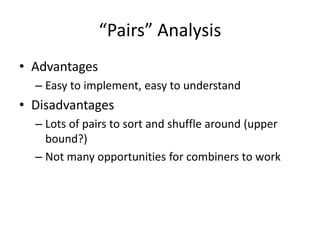
“Pairs” Analysis
• Advantages
– Easy to implement, easy to understand
• Disadvantages
– Lots of pairs to sort and shuffle around (upper
bound?)
– Not many opportunities for combiners to work
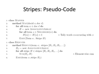
Another Try: “Stripes”
 Idea: group together pairs into an associative array
 Each mapper takes a sentence:
 Generate all co-occurring term pairs
 For each term, emit a → { b: countb, c: countc, d: countd … }
 Reducers perform element-wise sum of associative arrays
(a, b) → 1
(a, c) → 2
(a, d) → 5
(a, e) → 3
(a, f) → 2
a → { b: 1, c: 2, d: 5, e: 3, f: 2 }
a → { b: 1, d: 5, e: 3 }
a → { b: 1, c: 2, d: 2, f: 2 }
a → { b: 2, c: 2, d: 7, e: 3, f: 2 }
+
Stripes: Pseudo-Code
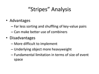
“Stripes” Analysis
• Advantages
– Far less sorting and shuffling of key-value pairs
– Can make better use of combiners
• Disadvantages
– More difficult to implement
– Underlying object more heavyweight
– Fundamental limitation in terms of size of event
space
Cluster size: 38 cores
Data Source: Associated Press Worldstream (APW) of the English Gigaword Corpus (v3),
which contains 2.27 million documents (1.8 GB compressed, 5.7 GB uncompressed)
Questions
• Can you combine “Stripes” approach with in-
mapper combiner?
• What if the stripes are too large?
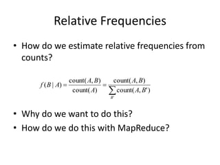
Relative Frequencies
• How do we estimate relative frequencies from
counts?
• Why do we want to do this?
• How do we do this with MapReduce?



'
)
'
,
(
count
)
,
(
count
)
(
count
)
,
(
count
)
|
(
B
B
A
B
A
A
B
A
A
B
f
f(B|A): “Stripes”
• Easy!
– One pass to compute (a, *)
– Another pass to directly compute f(B|A)
a → {b1:3, b2 :12, b3 :7, b4 :1, … }
f(B|A): “Pairs”
 For this to work:
 Must emit extra (a, *) for every bn in mapper
 Must make sure all a’s get sent to same reducer (use partitioner)
 Must make sure (a, *) comes first (define sort order)
 Must hold state in reducer across different key-value pairs
(a, b1) → 3
(a, b2) → 12
(a, b3) → 7
(a, b4) → 1
…
(a, *) → 32
(a, b1) → 3 / 32
(a, b2) → 12 / 32
(a, b3) → 7 / 32
(a, b4) → 1 / 32
…
Reducer holds this value in memory
“Order Inversion”
• Common design pattern
– Computing relative frequencies requires marginal counts
– But marginal cannot be computed until you see all counts
– Buffering is a bad idea!
– Trick: getting the marginal counts to arrive at the reducer
before the joint counts
• Optimizations
– Apply in-memory combining pattern to accumulate
marginal counts
– Should we apply combiners?
Synchronization: Pairs vs. Stripes
• Approach 1: turn synchronization into an ordering problem
– Sort keys into correct order of computation
– Partition key space so that each reducer gets the appropriate set
of partial results
– Hold state in reducer across multiple key-value pairs to perform
computation
– Illustrated by the “pairs” approach
• Approach 2: construct data structures that bring partial
results together
– Each reducer receives all the data it needs to complete the
computation
– Illustrated by the “stripes” approach
Recap: Tools for Synchronization
• Cleverly-constructed data structures
– Bring data together
• Sort order of intermediate keys
– Control order in which reducers process keys
• Partitioner
– Control which reducer processes which keys
• Preserving state in mappers and reducers
– Capture dependencies across multiple keys and
values
Issues and Tradeoffs
• Number of key-value pairs
– Object creation overhead
– Time for sorting and shuffling pairs across the network
• Size of each key-value pair
– De/serialization overhead
• Local aggregation
– Opportunities to perform local aggregation varies
– Combiners make a big difference
– Combiners vs. in-mapper combining
– RAM vs. disk vs. network

More Related Content

PPTX
Hadoop and Mapreduce for .NET User Group
PPT
Hadoop classes in mumbai
PPTX
Lecture2-MapReduce - An introductory lecture to Map Reduce
PPTX
This gives a brief detail about big data
PPTX
Enar short course
PPT
Map reduce - simplified data processing on large clusters
PPTX
Hadoop-part1 in cloud computing subject.pptx
PDF
ENAR short course
Hadoop and Mapreduce for .NET User Group
Hadoop classes in mumbai
Lecture2-MapReduce - An introductory lecture to Map Reduce
This gives a brief detail about big data
Enar short course
Map reduce - simplified data processing on large clusters
Hadoop-part1 in cloud computing subject.pptx
ENAR short course

Similar to MapReduce Algorithm Design - Parallel Reduce Operations (20)

PPTX
MapReduce
PDF
2 mapreduce-model-principles
PPTX
MapReduce.pptx
PPTX
COMPLETE MAP AND REDUCE FRAMEWORK INTRODUCTION
PPTX
Map reduce programming model to solve graph problems
PPTX
introduction to Complete Map and Reduce Framework
PPTX
Map reduce helpful for college students.pptx
PDF
PDF
Computing Scientometrics in Large-Scale Academic Search Engines with MapReduce
PPT
L19CloudMapReduce introduction for cloud computing .ppt
PPTX
mapreduce.pptx
PDF
module3part-1-bigdata-230301002404-3db4f2a4 (1).pdf
PPTX
Big Data.pptx
PPTX
Cloud infrastructure. Google File System and MapReduce - Andrii Vozniuk
PDF
MapReduce basics
PPTX
Introduction to MapReduce
PDF
(Berkeley CS186 guest lecture) Big Data Analytics Systems: What Goes Around C...
PPTX
Big Data Processing
PDF
Map Reducec and Spark big data visualization and analytics
PDF
Design patterns in MapReduce
MapReduce
2 mapreduce-model-principles
MapReduce.pptx
COMPLETE MAP AND REDUCE FRAMEWORK INTRODUCTION
Map reduce programming model to solve graph problems
introduction to Complete Map and Reduce Framework
Map reduce helpful for college students.pptx
Computing Scientometrics in Large-Scale Academic Search Engines with MapReduce
L19CloudMapReduce introduction for cloud computing .ppt
mapreduce.pptx
module3part-1-bigdata-230301002404-3db4f2a4 (1).pdf
Big Data.pptx
Cloud infrastructure. Google File System and MapReduce - Andrii Vozniuk
MapReduce basics
Introduction to MapReduce
(Berkeley CS186 guest lecture) Big Data Analytics Systems: What Goes Around C...
Big Data Processing
Map Reducec and Spark big data visualization and analytics
Design patterns in MapReduce
Ad

More from Jason J Pulikkottil (20)

PDF
Unix/Linux Command Reference - File Commands and Shortcuts
PDF
Introduction to PERL Programming - Complete Notes
PDF
VLSI System Verilog Notes with Coding Examples
PDF
VLSI Physical Design Physical Design Concepts
PDF
Verilog Coding examples of Digital Circuits
PDF
Floor Plan, Placement Questions and Answers
PDF
Physical Design, ASIC Design, Standard Cells
PDF
Basic Electronics, Digital Electronics, Static Timing Analysis Notes
PDF
Floorplan, Powerplan and Data Setup, Stages
PDF
Floorplanning Power Planning and Placement
PDF
Digital Electronics Questions and Answers
PDF
Different Types Of Cells, Types of Standard Cells
PDF
DFT Rules, set of rules with illustration
PDF
Clock Definitions Static Timing Analysis for VLSI Engineers
PDF
Basic Synthesis Flow and Commands, Logic Synthesis
PDF
ASIC Design Types, Logical Libraries, Optimization
PDF
Floorplanning and Powerplanning - Definitions and Notes
PDF
Physical Design Flow - Standard Cells and Special Cells
PDF
Physical Design - Import Design Flow Floorplan
PDF
Physical Design-Floor Planning Goals And Placement
Unix/Linux Command Reference - File Commands and Shortcuts
Introduction to PERL Programming - Complete Notes
VLSI System Verilog Notes with Coding Examples
VLSI Physical Design Physical Design Concepts
Verilog Coding examples of Digital Circuits
Floor Plan, Placement Questions and Answers
Physical Design, ASIC Design, Standard Cells
Basic Electronics, Digital Electronics, Static Timing Analysis Notes
Floorplan, Powerplan and Data Setup, Stages
Floorplanning Power Planning and Placement
Digital Electronics Questions and Answers
Different Types Of Cells, Types of Standard Cells
DFT Rules, set of rules with illustration
Clock Definitions Static Timing Analysis for VLSI Engineers
Basic Synthesis Flow and Commands, Logic Synthesis
ASIC Design Types, Logical Libraries, Optimization
Floorplanning and Powerplanning - Definitions and Notes
Physical Design Flow - Standard Cells and Special Cells
Physical Design - Import Design Flow Floorplan
Physical Design-Floor Planning Goals And Placement
Ad

Recently uploaded (20)

PPTX
Introduction-to-Cloud-ComputingFinal.pptx
PPTX
Moving the Public Sector (Government) to a Digital Adoption
PPTX
The THESIS FINAL-DEFENSE-PRESENTATION.pptx
PDF
22.Patil - Early prediction of Alzheimer’s disease using convolutional neural...
PPTX
Supervised vs unsupervised machine learning algorithms
PPTX
Introduction to Basics of Ethical Hacking and Penetration Testing -Unit No. 1...
PPTX
mbdjdhjjodule 5-1 rhfhhfjtjjhafbrhfnfbbfnb
PPTX
Data_Analytics_and_PowerBI_Presentation.pptx
PDF
Mega Projects Data Mega Projects Data
PPTX
Acceptance and paychological effects of mandatory extra coach I classes.pptx
PPTX
MODULE 8 - DISASTER risk PREPAREDNESS.pptx
PPTX
oil_refinery_comprehensive_20250804084928 (1).pptx
PPTX
CEE 2 REPORT G7.pptxbdbshjdgsgjgsjfiuhsd
PPTX
advance b rammar.pptxfdgdfgdfsgdfgsdgfdfgdfgsdfgdfgdfg
PDF
TRAFFIC-MANAGEMENT-AND-ACCIDENT-INVESTIGATION-WITH-DRIVING-PDF-FILE.pdf
PPTX
STUDY DESIGN details- Lt Col Maksud (21).pptx
PDF
Introduction to Business Data Analytics.
PDF
Fluorescence-microscope_Botany_detailed content
PPTX
Major-Components-ofNKJNNKNKNKNKronment.pptx
PPT
Chapter 3 METAL JOINING.pptnnnnnnnnnnnnn
Introduction-to-Cloud-ComputingFinal.pptx
Moving the Public Sector (Government) to a Digital Adoption
The THESIS FINAL-DEFENSE-PRESENTATION.pptx
22.Patil - Early prediction of Alzheimer’s disease using convolutional neural...
Supervised vs unsupervised machine learning algorithms
Introduction to Basics of Ethical Hacking and Penetration Testing -Unit No. 1...
mbdjdhjjodule 5-1 rhfhhfjtjjhafbrhfnfbbfnb
Data_Analytics_and_PowerBI_Presentation.pptx
Mega Projects Data Mega Projects Data
Acceptance and paychological effects of mandatory extra coach I classes.pptx
MODULE 8 - DISASTER risk PREPAREDNESS.pptx
oil_refinery_comprehensive_20250804084928 (1).pptx
CEE 2 REPORT G7.pptxbdbshjdgsgjgsjfiuhsd
advance b rammar.pptxfdgdfgdfsgdfgsdgfdfgdfgsdfgdfgdfg
TRAFFIC-MANAGEMENT-AND-ACCIDENT-INVESTIGATION-WITH-DRIVING-PDF-FILE.pdf
STUDY DESIGN details- Lt Col Maksud (21).pptx
Introduction to Business Data Analytics.
Fluorescence-microscope_Botany_detailed content
Major-Components-ofNKJNNKNKNKNKronment.pptx
Chapter 3 METAL JOINING.pptnnnnnnnnnnnnn

MapReduce Algorithm Design - Parallel Reduce Operations

  • 2. MapReduce: Recap • Programmers must specify: map (k, v) → <k’, v’>* reduce (k’, v’) → <k’, v’>* – All values with the same key are reduced together • Optionally, also: partition (k’, number of partitions) → partition for k’ – Often a simple hash of the key, e.g., hash(k’) mod n – Divides up key space for parallel reduce operations combine (k’, v’) → <k’, v’>* – Mini-reducers that run in memory after the map phase – Used as an optimization to reduce network traffic • The execution framework handles everything else…
  • 3. “Everything Else” • The execution framework handles everything else… – Scheduling: assigns workers to map and reduce tasks – “Data distribution”: moves processes to data – Synchronization: gathers, sorts, and shuffles intermediate data – Errors and faults: detects worker failures and restarts • Limited control over data and execution flow – All algorithms must expressed in m, r, c, p • You don’t know: – Where mappers and reducers run – When a mapper or reducer begins or finishes – Which input a particular mapper is processing – Which intermediate key a particular reducer is processing
  • 4. combine combine combine combine b a 1 2 c 9 a c 5 2 b c 7 8 partition partition partition partition map map map map k1 k2 k3 k4 k5 k6 v1 v2 v3 v4 v5 v6 b a 1 2 c c 3 6 a c 5 2 b c 7 8 Shuffle and Sort: aggregate values by keys reduce reduce reduce a 1 5 b 2 7 c 2 9 8 r1 s1 r2 s2 r3 s3
  • 5. Tools for Synchronization • Cleverly-constructed data structures – Bring partial results together • Sort order of intermediate keys – Control order in which reducers process keys • Partitioner – Control which reducer processes which keys • Preserving state in mappers and reducers – Capture dependencies across multiple keys and values
  • 6. Preserving State Mapper object configure map close state one object per task Reducer object configure reduce close state one call per input key-value pair one call per intermediate key API initialization hook API cleanup hook
  • 7. Scalable Hadoop Algorithms: Themes • Avoid object creation – Inherently costly operation – Garbage collection • Avoid buffering – Limited heap size – Works for small datasets, but won’t scale!
  • 8. Importance of Local Aggregation • Ideal scaling characteristics: – Twice the data, twice the running time – Twice the resources, half the running time • Why can’t we achieve this? – Synchronization requires communication – Communication kills performance • Thus… avoid communication! – Reduce intermediate data via local aggregation – Combiners can help
  • 9. Shuffle and Sort Mapper Reducer other mappers other reducers circular buffer (in memory) spills (on disk) merged spills (on disk) intermediate files (on disk) Combiner Combiner
  • 10. Word Count: Baseline What’s the impact of combiners?
  • 11. Word Count: Version 1 Are combiners still needed?
  • 12. Word Count: Version 2 Are combiners still needed?
  • 13. Design Pattern for Local Aggregation • “In-mapper combining” – Fold the functionality of the combiner into the mapper by preserving state across multiple map calls • Advantages – Speed – Why is this faster than actual combiners? • Disadvantages – Explicit memory management required – Potential for order-dependent bugs
  • 14. Combiner Design • Combiners and reducers share same method signature – Sometimes, reducers can serve as combiners – Often, not… • Remember: combiner are optional optimizations – Should not affect algorithm correctness – May be run 0, 1, or multiple times • Example: find average of all integers associated with the same key
  • 15. Computing the Mean: Version 1 Why can’t we use reducer as combiner?
  • 16. Computing the Mean: Version 2 Why doesn’t this work?
  • 17. Computing the Mean: Version 3 Fixed?
  • 18. Computing the Mean: Version 4 Are combiners still needed? What if the S & C are too large?
  • 19. Algorithm Design: Running Example • Term co-occurrence matrix for a text collection – M = N x N matrix (N = vocabulary size) – Mij: number of times i and j co-occur in some context (for concreteness, let’s say context = sentence) • Why? – Distributional profiles as a way of measuring semantic distance – Semantic distance useful for many language processing tasks
  • 20. MapReduce: Large Counting Problems • Term co-occurrence matrix for a text collection = specific instance of a large counting problem – A large event space (number of terms) – A large number of observations (the collection itself) – Goal: keep track of interesting statistics about the events • Basic approach – Mappers generate partial counts – Reducers aggregate partial counts How do we aggregate partial counts efficiently?
  • 21. First Try: “Pairs” • Each mapper takes a sentence: – Generate all co-occurring term pairs – For all pairs, emit (a, b) → count • Reducers sum up counts associated with these pairs • Use combiners!
  • 23. “Pairs” Analysis • Advantages – Easy to implement, easy to understand • Disadvantages – Lots of pairs to sort and shuffle around (upper bound?) – Not many opportunities for combiners to work
  • 24. Another Try: “Stripes”  Idea: group together pairs into an associative array  Each mapper takes a sentence:  Generate all co-occurring term pairs  For each term, emit a → { b: countb, c: countc, d: countd … }  Reducers perform element-wise sum of associative arrays (a, b) → 1 (a, c) → 2 (a, d) → 5 (a, e) → 3 (a, f) → 2 a → { b: 1, c: 2, d: 5, e: 3, f: 2 } a → { b: 1, d: 5, e: 3 } a → { b: 1, c: 2, d: 2, f: 2 } a → { b: 2, c: 2, d: 7, e: 3, f: 2 } +
  • 26. “Stripes” Analysis • Advantages – Far less sorting and shuffling of key-value pairs – Can make better use of combiners • Disadvantages – More difficult to implement – Underlying object more heavyweight – Fundamental limitation in terms of size of event space
  • 27. Cluster size: 38 cores Data Source: Associated Press Worldstream (APW) of the English Gigaword Corpus (v3), which contains 2.27 million documents (1.8 GB compressed, 5.7 GB uncompressed)
  • 28. Questions • Can you combine “Stripes” approach with in- mapper combiner? • What if the stripes are too large?
  • 29. Relative Frequencies • How do we estimate relative frequencies from counts? • Why do we want to do this? • How do we do this with MapReduce?    ' ) ' , ( count ) , ( count ) ( count ) , ( count ) | ( B B A B A A B A A B f
  • 30. f(B|A): “Stripes” • Easy! – One pass to compute (a, *) – Another pass to directly compute f(B|A) a → {b1:3, b2 :12, b3 :7, b4 :1, … }
  • 31. f(B|A): “Pairs”  For this to work:  Must emit extra (a, *) for every bn in mapper  Must make sure all a’s get sent to same reducer (use partitioner)  Must make sure (a, *) comes first (define sort order)  Must hold state in reducer across different key-value pairs (a, b1) → 3 (a, b2) → 12 (a, b3) → 7 (a, b4) → 1 … (a, *) → 32 (a, b1) → 3 / 32 (a, b2) → 12 / 32 (a, b3) → 7 / 32 (a, b4) → 1 / 32 … Reducer holds this value in memory
  • 32. “Order Inversion” • Common design pattern – Computing relative frequencies requires marginal counts – But marginal cannot be computed until you see all counts – Buffering is a bad idea! – Trick: getting the marginal counts to arrive at the reducer before the joint counts • Optimizations – Apply in-memory combining pattern to accumulate marginal counts – Should we apply combiners?
  • 33. Synchronization: Pairs vs. Stripes • Approach 1: turn synchronization into an ordering problem – Sort keys into correct order of computation – Partition key space so that each reducer gets the appropriate set of partial results – Hold state in reducer across multiple key-value pairs to perform computation – Illustrated by the “pairs” approach • Approach 2: construct data structures that bring partial results together – Each reducer receives all the data it needs to complete the computation – Illustrated by the “stripes” approach
  • 34. Recap: Tools for Synchronization • Cleverly-constructed data structures – Bring data together • Sort order of intermediate keys – Control order in which reducers process keys • Partitioner – Control which reducer processes which keys • Preserving state in mappers and reducers – Capture dependencies across multiple keys and values
  • 35. Issues and Tradeoffs • Number of key-value pairs – Object creation overhead – Time for sorting and shuffling pairs across the network • Size of each key-value pair – De/serialization overhead • Local aggregation – Opportunities to perform local aggregation varies – Combiners make a big difference – Combiners vs. in-mapper combining – RAM vs. disk vs. network