Indifference Curve Analysis
Ordinal Approach or
The concept of Scale of Preferences or
The Indifference Curve Technique
• Originated by Edgeworth in 1881 and
Refined by Pareto in 1906.
• Application in the demand analysis at
the hands of J.R. HICKS and R.G.D
.Allen in 1934.
The Ordinal Approach In Utility Theory

•

•
•

•

•

The ordinal theory suggests that
utility is only relatively discernible
but not quantifiable.
U is the level of satisfaction than
an amount of satisfaction.
Utility is a series of assigned
numbers to rank options by the
consumer preference. The
assigned numbers reveal what is
more preferred but cannot tell
how much the difference is.
Utility can only be ranked by an
order or a scale of preference to
show the degree of willingness of
a consumer.
Hicks uses ‘Significance’ rather
than ’Utility’.

Combinations
between Apples
and Bananas

Level of
Satisfaction
Derived

Ranking
Order of
Preference

a)

12 Apples
+
12 Bananas

Highest

First

b)

10 Apples
+
19 Bananas

Lesser than
(a)

Second

c)

5 Apples
+
5 Bananas

Lesser than
(b)

Third
Scale of Preferences - Characteristics
• Drawn by a consumer in his mind consciously or
unconsciously.
• Based on subjective valuation of goods made by the
customer on the basis of his liking, habits, tastes,
desires, intensity of wants, etc.
• Independent of Price and consumer’s income.
• It represents Ordinal comparison of the level of
satisfaction derived by the consumer from different
combinations of goods.
• Scale of Preferences differs from person to person.
• Scale of Preferences considers the significance of the
commodity in the context of their stocks.
Definitions
• Indifference Schedule —An Indifference schedule is a
list of alternate combinations in the stocks of two goods
which yield equal satisfaction to the consumer.
• Indifference Curve- An Indifference curve is the locus of
points representing all the different combinations if the
two goods (say X and Y) which yield equal utility or
satisfaction to the consumer.
• Indifference Map- A graph showing a whole set of
indifference curves is called an indifference map. All
points on the same curve give equal level of satisfaction,
but each point on higher curve gives higher level of
satisfaction.
Indifference Curve Analysis
• The indifference
curve analysis is a
technique for
explaining how
choices between
two alternatives
are made.

Indifference Schedule
Combinati Apples
on

Mangoes

A

15

1

B

11

2

C

8

3

D

6

4

E

5

5
Indifference Curve & Map
Indifference Curve

Indifference Map
Y

Y

a
a’

A
B

a”

C
IC

IC
0

b b’ b”

X

0

IC
IC
X
Hypothetical data for an IC Map

Combination of Goods
(Units)
I

II

Y

III

Y

X

Y

X

Y

1

10

2

15

3

20

2

6

4

10

5

14

3

3

6

6

7

7

4

1

8

3

9

QT of comm Y

X

a

c

7

∙

U1(IC1)

U2(IC2)

U3(IC3)

Third Order
Preference

Second Order
Preference

First Order
Preference

U3
b

d
U2
U1

O
QT of comm X

X
ASSUMPTIONS
• A consumer is interested in buying two goods in combination.
• He is able to rank his preferences & give a complete ordering
of the scale of preferences.
• Non-satiation, i.e, the consume always prefers more
quantities of goods to lesser quantities.
• He is rational and his choices are transitive.It means, if he
prefers combination a to b and b to c, then he must also prefer
a to c.
• Height of the IC indicates the level of satisfaction.
• IC are drawn as continuous curves assuming infinitesimal
amount of changes in the combination of 2 goods i.e. perfect
division of the goods under consideration.
The Indifference Curve Theory
Based on these assertions, Edgeworth F.
Y. ( 1845 - 1926 ) first suggested the
indifference curve to represent the level of
preference a consumer has when two
goods are consumed with different
amount, but each combination of these
two goods yields the same level of
satisfaction.
The Properties of the Indifference Curve

• IC slopes downwards from left to right , i.e.
negatively sloped, indicating if X increases
in combination X and Y , there should be a
decrease in Y amount to be on the same
level of satisfaction.
• They are convex to origin.
• They can’t intersect each other.
Indifference curves slope down from left to right.

clothing

A

C

B

food

Consider 2 points A & B on the
same indifference curve.
At point B, you have more food
than at point A.
If the amount of clothing you had
at point B was the same as or
more than at point A (like at
point C), you would not be
indifferent between A and B
(since more is better).
So A & B could not be on the
same indifference curve, which
goes against our initial statement
that they are.
So you must have less clothing
at B, which means than B lies
below A and the indifference
curve slopes downward.
Indifference curves to the northeast are preferred.

clothing
E
A

IC2

IC1
foo
d

Point E is preferred to
point A because it has
more food & more
clothing.
Since you are indifferent
between A & all points
on IC1, E must be
preferred to all points on
IC1.
Since you are indifferent
between E and all
points on IC2, all points
on IC2 must be preferred
to all points on IC1.
Indifference Curves: Shape
• The indifference curves are not likely to be vertical,
horizontal, or upward sloping.
– A vertical or horizontal indifference curve holds the quantity of
one of the goods constant, implying that the consumer is
indifferent to getting more of one good without giving up any of
the other good.
– An upward-sloping curve would mean that the consumer is
indifferent between a combination of goods that provides less of
everything and another that provides more of everything.
– Rational consumers usually prefer more to less.
14
Copyright © Houghton Mifflin Company. All rights
reserved.
Indifference Curve Shapes

15
Copyright © Houghton Mifflin Company. All rights
reserved.
Indifference Curves: Slope
• The slope or steepness of indifference curves is
determined by consumer preferences.
– It reflects the amount of one good that a consumer must give
up to get an additional unit of the other good while remaining
equally satisfied.
– This relationship changes according to diminishing marginal
utility—the more a consumer has of a good, the less the
consumer values an additional value of that good. Convexity
implies diminishing slope of the indifference curve.

16
Copyright © Houghton Mifflin Company. All rights
reserved.
Indifference curves can not intersect.

clothing

Suppose indifference curves could intersect.
Let the intersection of IC1 & IC2 be D.
Then you must be indifferent between D &
any other point A on IC1.
Similarly, you must be indifferent between D
& any other point B on IC2.
By transitivity, you must be
indifferent between A & B.
But A & B are not on the same
D
indifference curve, which they
B IC2 should be if you are indifferent
between them.
Then, our initial supposition that
IC1
A
indifference curves could
intersect must be wrong.
foo
d
Indifference curves are convex
[the slopes of IC’s fall as we move from left to right, or
we have a diminishing marginal rate of substitution (MRS)]
clothing

A
B

C D

foo
d

When we have lots of
clothing & not much food
(as near A & B), we are
willing to give up a lot of
clothing to get a little
more food.
When we have lots of
food & not much clothing
(as near C & D), we are
willing to give up very
little clothing to get a
little more food.
Odd special cases that are not
consistent with the properties of
Indifference curve listed previously.
Perfect Complements
tyres

IC2

8

IC1
4

1

2

Car
bodies

You need exactly 4 tyres
with 1 car body
(ignoring the spare
tyre).
Having more than 4 tyres
with 1 car body doesn’t
increase utility.
Also having more than 1
car body with only 4
tyres doesn’t increase
utility either.
Perfect Substitutes
Minipacks
10

5
IC1
1

IC2

2

Jumb
o
pack
s

Consider two packs of paper;
the mini-pack has 100 sheets &
the jumbo pack has 500 sheets.
No matter how many mini-packs
or jumbo packs you have, you
are always willing to trade 5
mini-packs for 1 jumbo pack.
Since the rate at which you’re
willing to trade is the slope of
the IC, and that rate is constant,
your IC’s have a constant slope.
That means they are straight
lines.
“Neutral” Good
Neutral
good
IC1
IC3

IC2

Your utility is unaffected
by consumption of a
neutral good.

Desire
d good
The Marginal Rate of Substitution
• Def: The MRS of Xof Y refers to the amount
of Y that must be given up per unit of X
gained by the consumer to keep the level if
satisfaction unchanged.
• MRSxy= y/ x, where
• MRSxy = the MRs of X for Y
• Y = a small change in the quantity of Y
•
X = a small change in the quantity of X
The slope of the indifference
curve is the rate at which you
are willing to trade off one good
to get another good.

It is called the marginal rate of substitution
or MRS.
What is the MRS or slope of the
IC? points A & B are on the same
Suppose
Clothing C
indifference curve & therefore have the
same utility level.
IC2
Let’s break up the move from A to B
IC1
into 2 parts.
A
A→D: ∆TU = ∆C (MUC)
D→B: ∆TU = ∆F (MUF)
B
A→B:
D
0 = ∆TU = ∆C (MUC) + ∆F (MUF)
⇒ ∆C (MUC) = – ∆F (MUF)
⇒ ∆C/∆F = – MUF / MUC
Food F
So along an indifference curve, the slope or MRS is the
negative of the ratio of the marginal utilities (with the MU of the
good on the horizontal axis in the numerator).
MRS = – MUX / MUY
For example,
Clothing C
IC1 =90

IC2 =
96
A

6

5

D
7

Suppose IC1 is the 90-util indifference
curve & IC2 is the 96-util indifference
curve.
Point A is 7 units of food & 6 of
clothing.
B is 9 units of food & 5 of clothing.
Since an additional unit of clothing
gives you 6 more utils of satisfaction,
the MU of clothing must be 6.
B
Since an additional 2 units of food
also give you 6 more utils of
satisfaction, the MU of food must be
9Food F 3.
So, MRS = – MUF / MUC = -3/6 = -0.5 .
You’d give up 2 units of food to get
1 units of clothing.
•Hicks replaces the law
of DMU by the principle
of Diminishing
Marginal Rate of
Substitution.
•As the consumer
increases the quantity
of X then its MU
decreases and % of
substitution will be less
as the point moves
downwards on the IC
curve

Comm Y

Comm X

MRS =
y / x

10

25

-

11

20

-5/1=-5

12

16

-4/1=-4

13

13

-3/1=-3

14

11

-2/1=-2
Budget Constraint Or Budget Line or
Price Line
• DEF: The Budget line is the locus of points
representing all the different combinations of the two
goods that can be purchased by the consumer, given
his money income and the prices of the two goods.
• What a consumer can actually buy depends on the
income at his disposal and the prices of goods he
wants to buy.
• Income and Price are 2 objective factors which form
the budgetary constraint of the consumer.
• The consumption or purchase possibility of the
consumer is restricted to the budget constraint.
Contd…
• The slope of the budget line is called the marginal
rate of substitution in exchange = PX / PY.
• The concept of relative price is important because a
rise in relative price would encourage the producer
to put more resources in production. The concept
also conveys the market information of relative
scarcity of those resources.
• The budget line rotates when the relative price
changes.
• The shift of the line means that either the income
changes or there is a change in the price of both
goods.
Alternate Purchase
Possibilities

Given income = Rs. 50
If P of Y = Rs 10/ unit
If P of X = Rs 5/ unit
AB= Budget
( Price, Income) Line

Units
of Y

Qt of Y

a
b
c
s

B
O

Qt of x

B

X

4
6

1

z

2

2

A

0

3

Y

5
4

A

Units
of X

8

0

10
Budget Constraint or Budget
Line
This equation tells you what you can buy.
For example, suppose you have $24, & there are
two goods.
The price of the first good is $3 per unit & the price
of the second good is $4 per unit.
So, if you buy X units of the first good for $3 each,
you spend 3X on that good.
Similarly, if you buy Y units of the second good, you
spend 4Y on that good.
Your total spending is 3X+4Y.
If you spend all 24 dollars that you have, 3X+4Y=24.
That equation is your budget constraint.
Example: Budget constraint for $24 of income,
and $3 & $4 for the prices of the two goods.

Y

(0,
6)

0

If you spent all $24 on the 1st good,
you could buy 8 units.
If you spent all $24 on the 2nd good,
you could buy 6 units.
So we have the intercepts of the
budget constraint.
The slope of the line connecting these
two points is
∆Y/∆X = – 6/8 = – 3/4 = – 0.75 .

(8,0
)

X
Let’s generalize. Keep in mind that income was $24
and the prices of the goods were $3 & $4. The equation of
the budget constraint in our example was 3X + 4Y = 24.
So the budget constraint is p1X + p2Y = I
Solving for Y in terms of X, p2Y = I – p1X,
or Y = I /p2 – (p1/p2)X

Y

(0,
6)

0

So from our slope-intercept form, we see that
the intercept is I /p2, and the slope is –p1/p2 .
The intercept is income divided by the price of
the good on the vertical axis.
The slope is the negative of the ratio of
the prices, with the price of the good
on the horizontal axis in the
numerator.
(8,0
)

X
We have the intercept I /p2,
& the slope is –p1/p2 .

Y
(0,
9)
(0,
6)

0

What if income increased?
The slope would stay the same & the budget constraint
would shift out parallel to the original one.
Suppose in our example with income of 24 & prices of
3 & 4, income increased to 36.
Our new y-intercept will be 36/4 =9
& the new X-intercept will be 36/3=12.

(8,0 (12,0
)
) X
Suppose the price of the good on the X-axis increased.

Y

(0,
6)

0

If we bought only the good whose price
increased, we could afford less of it.
If we bought only the other good, our
purchases would be unchanged.
So the budget constraint would pivot inward
about the Y-intercept.
For example, if the price increased
from $3 to $4, our $24 would only
buy 6 units.

(6,0)

(8,0
)

X
Similarly, if the price of the good on the Yaxis increased, the budget constraint would
pivot in about the X-intercept.
Y

(0,
6)
(0,4)

0

Suppose the price of the 2nd good
increased from $4 to $6. If you bought
only that good, with your $24, your $24
would only buy 4 units of it.

(8,0
)

X
Y

Y

A3

Changes in Income.

A2

Px, Py constant

A1

Comm of Y

Comm of Y

A1

O

Changes in
Price of X

B1 B2 B3

X

Comm of X

O

B1

B2

B3

Comm of X

A2

Changes in
Price of Y

Comm of Y

A1
Changes in
money income,
Prices
and the BL

O

X

Comm of X

B
Let’s combine our indifference curves &
budget constraint to determine our utility
maximizing point.
Y
IC1

IC2

IC3

Point A doesn’t maximize
our utility & it doesn’t
spend all our income.
(It’s below the budget
constraint.)

A

0

X
Y
IC1

IC2

IC3

Points B & C spend all our
income but they don’t maximize
our utility. We can reach a
higher indifference curve.

B

C
0

X
Point D is unattainable. We
can’t reach it with our budget.
Y
IC1

IC2

IC3
D

0

X
Y
IC1

IC2

Point E is our utility-maximizing point.
We can’t do any better than at E.
Notice that our utility is maximized at
the point of tangency between the
budget constraint & the indifference
curve.

IC3

E

0

X
Assumptions of the Consumer Equilibrium
• Consumer
•
•
•
•

Has fixed amount of money income.
Intends to buy combination of 2 goods, X and Y.
Has definite tastes and preferences.
Hence has definite scale of preferences. Expressed
through ICM.
• S of P remains same through out the analysis.
• Is rational and mazimizes his satisfaction

• Each of the goods X and Y is homogenous
(identical characteristics) and divisible, so
various combinations of these goods can
be sold.
The consumer Equilibrium

Qt. of comm Y

 Point e is the
a

M

e

b
N
Qt. of comm X

equilibrium
point given the
Budget line.
 Satisfaction
is max
when the MRS
of x for
y is just equal
to the price
of x to the
price of y.
Consumer Optimum or Equilibrium
• In mathematics, the slopes of the indifference
curve and the budget line are the same.
• Slope of the budget line = M R S in exchange
= PX / PY
• Slope of the indifference curve
= M R S in
consumption =
∆Y/∆X
•

In equilibrium, PX / PY = ∆ Y / ∆ X
What happens to consumption when income
rises?
For normal goods, consumption increases.
For inferior goods, consumption decreases.
What does this look like on our graph?
Two Normal Goods

Y

IC2

IC3

IC1
C
Y3
Y2

B

As income increases, the
budget constraint shifts out
& we are able to reach
higher & higher IC’s.
The points of tangency are
at higher & higher levels of
consumption of both
goods.

A

Y1
X1 X2
X3

X
Income-Consumption Curve

Y

IC2

IC3

IC1
C
Y3
Y2

B

The curve that traces out
these points is called the
income-consumption curve.
For two normal goods, the
curve slopes upward.
It may be convex (as drawn
here), concave, or linear.

A

Y1
X1 X2
X3

X
We can also look at consumption levels of two
goods when the price of one of them changes.

Y

Suppose there is an increase in the price
of the 1st good (the good on the X-axis).
The budget constraint pivots inward.
Here we see X drop & Y increase.
In this case, our 2 goods are
substitutes.

Y3
Y2
Y1
X3
X1

X2

X
If we connect the points, we have the
price consumption curve.
It shows the utility-maximizing
points when the price of a
good changes.

Y

Y3
Y2
Y1
X3
X1

X2

X
If we look at the price of a good & the amount
of it consumed, we have the demand curve
for our particular individual.
P

As the price decreases the
quantity demanded
increases & vice versa.

P1
P2
P3
X1 X2
X3

X
We can separate the effect of a change in the price of
a good on its consumption level into two parts:
the income effect & the substitution effect.

Y

YB
YA

B

XB
XA

A

Suppose the price of the
first good increases.
The budget constraint was
originally the blue line and
we were at A consuming
quantities XA & YA.
After the price change, the
budget constraint is the red
line, and we’re at B
consuming XB & YB .
X
We first want to capture the effect of the price change
without the effect of the change in income.

Y

H
YH
YB
YA

B

XB XH
XA

A

We draw a line parallel to the new budget
constraint and tangent to the old indifference
curve.
This will reflect the new relative prices, but since
we are tangent to the old indifference curve we
are just as well off as initially.
Under those circumstances we would be at point
H (for hypothetical).
Since the 1st good is now relatively more
expensive compared to the 2nd, we will
substitute, increasing Y & decreasing X.

X
The movement from A to H is the
substitution effect.
As a result of the increase in the relative
price of the 1st good, we reduce our
consumption of it and consume more of
the other good.

Y

H
YH
YB
YA

B

XB XH
XA

A

X
Now we move from H to B

Y

H
YH
YB
YA

B

XB XH
XA

A

Our purchasing power has been reduced by
the price change. That results in the income
effect.
In our graph, we now hold the relative prices
constant at the new level, but income has
fallen. Our budget constraint has shifted
inward.
If both goods are normal, as a result of the
change in income, we reduce our consumption
of both goods, and X & Y fall.
This is the income effect of the price change.

X
Total Effect of Price Increase
The total effect is to move from A to B.
X has fallen.
Both the substitution & income effects led to a
drop in X.
Y has increased in this case.
The substitution effect increased consumption
of the 2nd good, but the income effect reduced
it by less than the substitution effect increased
it.

Y

H
YH
YB
YA

B

XB XH
XA

A

X
Let’s do a price decrease.

Y

B

YB
YA

A

The budget constraint moves from the blue line
to the red line.
We draw a line parallel to the new budget
constraint and tangent to the old indifference
curve.
H is the tangency of the hypothetical budget
constraint with the old indifference curve.
The substitution effect is the movement from A
to H.
We substitute increasing X & decreasing Y.

H

YH
XA XH XB

X
The movement from H to B is the income effect.
As a result of the higher income (greater
purchasing power), we consume more of both
goods, if they are normal goods.

Y

B

YB
YA

A

H

YH
XA XH XB

X
Total Effect
The total effect is to move from A to B.
X has increased.
Both the substitution & income effects led to an
increase in X.
Y has also increased in this case.
The substitution effect decreased consumption
of the 2nd good, but the income effect
increased it by more than the substitution
effect decreased it.

Y

B

YB
YA

A

H

YH
XA XH XB

X
Income and Substitution Effects, in words
The income effect is the result of the change in purchasing
power.
If the price of a normal good increases, you feel poorer,
and the income effect is to consume less.
If the price of a normal good decreases, you feel richer,
and the income effect is to consume more.
The substitution effect is the result of a change in relative
prices.
If the price of a good increases, the substitution effect is to
consume less of it & more of the other goods that are
now relatively cheaper.
If the price decreases, the substitution effect is to consume
more of it & less of the goods that are now relatively
more expensive.

More Related Content

PPT
Indifference curve
PPTX
Indifference Curve
PPTX
Indifference Curves
PDF
Cardinal and ordinal utility a theory of consumer bheahviour
PPT
Indifference Curve Analysis PPT
PPTX
Cardinal utility analysis
PPTX
Bba 1 be 1 u-3 consumer behavior and demand analysis
PPT
7 utility
Indifference curve
Indifference Curve
Indifference Curves
Cardinal and ordinal utility a theory of consumer bheahviour
Indifference Curve Analysis PPT
Cardinal utility analysis
Bba 1 be 1 u-3 consumer behavior and demand analysis
7 utility

What's hot (20)

PDF
Utility analysis by Dr. ruchi jain
PPTX
Consumer Surplus
PDF
Demand analysis
PPTX
demand curve
PPTX
Utility analysis(2)
PPTX
Monopolistic competition
PPTX
Propreties of indifference curves
PPTX
Law of.Supply
PDF
Indifference curve analysis
PPTX
Consumer surplus
PPTX
Monopolistic Equilibrium in short and long run
PPTX
Price discrimination
PPTX
theory of cost
PPT
PPTX
Production function ppt in economics
PPTX
Cross elasticity of demand
PPTX
Unit- 2 Lecture-3 (comparative advantage theory)
PPTX
Terms of-trade
PPT
cardinal and ordinal utility analysis.
PPTX
Lecture 3
Utility analysis by Dr. ruchi jain
Consumer Surplus
Demand analysis
demand curve
Utility analysis(2)
Monopolistic competition
Propreties of indifference curves
Law of.Supply
Indifference curve analysis
Consumer surplus
Monopolistic Equilibrium in short and long run
Price discrimination
theory of cost
Production function ppt in economics
Cross elasticity of demand
Unit- 2 Lecture-3 (comparative advantage theory)
Terms of-trade
cardinal and ordinal utility analysis.
Lecture 3
Ad

Viewers also liked (20)

PPTX
Ordinal utility Managerial Economics
PPTX
Indifference curves
PPTX
Utility and cardinal utility analysis
PPT
Utility analysis ppt
PPT
Indifference curves
PPTX
Cardinal utility
PDF
Microeconomics: Income and Substitution Effects
PPTX
law of diminishing Marginal utility
PDF
Indifference Curve
PPTX
Chapter 21 consumer behavior and utility maximization
PPT
Income And Substitution Effect
PPTX
Consumer equilibrium under indifference curve analysis
PPT
Indifrrence curve analysis
PPTX
Theory Of Consumer Behavior
PPTX
Budget line
PPTX
4.2indifference curve
PPTX
Indifference curve
PPT
Indifferencecurve 121117043142-phpapp01
PPT
Indifference curve
PPT
Consumer2 behaviour indifference curve
Ordinal utility Managerial Economics
Indifference curves
Utility and cardinal utility analysis
Utility analysis ppt
Indifference curves
Cardinal utility
Microeconomics: Income and Substitution Effects
law of diminishing Marginal utility
Indifference Curve
Chapter 21 consumer behavior and utility maximization
Income And Substitution Effect
Consumer equilibrium under indifference curve analysis
Indifrrence curve analysis
Theory Of Consumer Behavior
Budget line
4.2indifference curve
Indifference curve
Indifferencecurve 121117043142-phpapp01
Indifference curve
Consumer2 behaviour indifference curve
Ad

Similar to Ordinal Utility Approach IC Curve (20)

PPTX
Indifference Curve -Managerial Economics
PPTX
indifference curve analysis: ordinal approach theory.pptx
PPTX
Indifference curve analysis
PDF
Indiffernece Curve Analysis.pdf
PPTX
unit 7: basic economics goods and services
PDF
economics production function presentation alevel
PPTX
Indiffrence-curve
PDF
Answer - 5A_indifference-curve-analysis.pdf
PPTX
indifference-curve-analysis.pptx NOTES
PPTX
indifference-curve-analysis concept.....
PPT
Indifference Curve
PPTX
Utilityffvhgg Analysis-Ordinal Approach.pptx
PPTX
Indifference Curve Theory | indifference curve | indifferece curve graph
PDF
Ordinal utility indifference curve properties and MRS
PPT
Indifference curve analysis ordinal utility approach
PPTX
INDIFFERENCE CURVES.pptx
PPTX
indifference-curve-analysis and properties.pptx
PPTX
Presentation on Indifference Curve
PPTX
Sldes of ECONA 101 ghty vftt frresd gttr
PPTX
Indifference curve
Indifference Curve -Managerial Economics
indifference curve analysis: ordinal approach theory.pptx
Indifference curve analysis
Indiffernece Curve Analysis.pdf
unit 7: basic economics goods and services
economics production function presentation alevel
Indiffrence-curve
Answer - 5A_indifference-curve-analysis.pdf
indifference-curve-analysis.pptx NOTES
indifference-curve-analysis concept.....
Indifference Curve
Utilityffvhgg Analysis-Ordinal Approach.pptx
Indifference Curve Theory | indifference curve | indifferece curve graph
Ordinal utility indifference curve properties and MRS
Indifference curve analysis ordinal utility approach
INDIFFERENCE CURVES.pptx
indifference-curve-analysis and properties.pptx
Presentation on Indifference Curve
Sldes of ECONA 101 ghty vftt frresd gttr
Indifference curve

More from Tej Kiran (20)

PPTX
Transactional Analysis and Communction
PPTX
Organizational communication
PPTX
Leadership
PPTX
Leadership and group
PPTX
Leadership
PPTX
Internal and external
PPTX
Barriers in communication
PPT
communtication
PPT
Partnership accounts
PDF
Basics of company accounts and issue of shares
DOCX
Amalgamation and absorption
PDF
Cash flow statement
PPT
Water resources in india
PPT
Solid waste
PPTX
Role of govt in environment
PPTX
Population growth & its effect on environment
PPT
Noise pollution
PPTX
Natural resources
PPTX
PPTX
Environmental activism
Transactional Analysis and Communction
Organizational communication
Leadership
Leadership and group
Leadership
Internal and external
Barriers in communication
communtication
Partnership accounts
Basics of company accounts and issue of shares
Amalgamation and absorption
Cash flow statement
Water resources in india
Solid waste
Role of govt in environment
Population growth & its effect on environment
Noise pollution
Natural resources
Environmental activism

Recently uploaded (20)

PPTX
Understanding Procurement Strategies.pptx Your score increases as you pick a ...
DOCX
Center Enamel Powering Innovation and Resilience in the Italian Chemical Indu...
PPTX
chapter 2 entrepreneurship full lecture ppt
PPTX
TRAINNING, DEVELOPMENT AND APPRAISAL.pptx
PPT
Retail Management and Retail Markets and Concepts
PPTX
Transportation in Logistics management.pptx
PPTX
33ABJFA6556B1ZP researhchzfrsdfasdfsadzd
PPTX
df0ee68f89e1a869be4bff9b80a7 business 79f0.pptx
PPTX
operations management : demand supply ch
PPTX
CTG - Business Update 2Q2025 & 6M2025.pptx
PDF
1911 Gold Corporate Presentation Aug 2025.pdf
PDF
Sustainable Digital Finance in Asia_FINAL_22.pdf
DOCX
Hand book of Entrepreneurship 4 Chapters.docx
PDF
THE COMPLETE GUIDE TO BUILDING PASSIVE INCOME ONLINE
PDF
HQ #118 / 'Building Resilience While Climbing the Event Mountain
DOCX
Center Enamel A Strategic Partner for the Modernization of Georgia's Chemical...
PDF
Highest-Paid CEO in 2025_ You Won’t Believe Who Tops the List.pdf
PPTX
IMM.pptx marketing communication givguhfh thfyu
PDF
Second Hand Fashion Call to Action March 2025
PDF
Stacey L Stevens - Canada's Most Influential Women Lawyers Revolutionizing Th...
Understanding Procurement Strategies.pptx Your score increases as you pick a ...
Center Enamel Powering Innovation and Resilience in the Italian Chemical Indu...
chapter 2 entrepreneurship full lecture ppt
TRAINNING, DEVELOPMENT AND APPRAISAL.pptx
Retail Management and Retail Markets and Concepts
Transportation in Logistics management.pptx
33ABJFA6556B1ZP researhchzfrsdfasdfsadzd
df0ee68f89e1a869be4bff9b80a7 business 79f0.pptx
operations management : demand supply ch
CTG - Business Update 2Q2025 & 6M2025.pptx
1911 Gold Corporate Presentation Aug 2025.pdf
Sustainable Digital Finance in Asia_FINAL_22.pdf
Hand book of Entrepreneurship 4 Chapters.docx
THE COMPLETE GUIDE TO BUILDING PASSIVE INCOME ONLINE
HQ #118 / 'Building Resilience While Climbing the Event Mountain
Center Enamel A Strategic Partner for the Modernization of Georgia's Chemical...
Highest-Paid CEO in 2025_ You Won’t Believe Who Tops the List.pdf
IMM.pptx marketing communication givguhfh thfyu
Second Hand Fashion Call to Action March 2025
Stacey L Stevens - Canada's Most Influential Women Lawyers Revolutionizing Th...

Ordinal Utility Approach IC Curve

  • 2. Ordinal Approach or The concept of Scale of Preferences or The Indifference Curve Technique • Originated by Edgeworth in 1881 and Refined by Pareto in 1906. • Application in the demand analysis at the hands of J.R. HICKS and R.G.D .Allen in 1934.
  • 3. The Ordinal Approach In Utility Theory • • • • • The ordinal theory suggests that utility is only relatively discernible but not quantifiable. U is the level of satisfaction than an amount of satisfaction. Utility is a series of assigned numbers to rank options by the consumer preference. The assigned numbers reveal what is more preferred but cannot tell how much the difference is. Utility can only be ranked by an order or a scale of preference to show the degree of willingness of a consumer. Hicks uses ‘Significance’ rather than ’Utility’. Combinations between Apples and Bananas Level of Satisfaction Derived Ranking Order of Preference a) 12 Apples + 12 Bananas Highest First b) 10 Apples + 19 Bananas Lesser than (a) Second c) 5 Apples + 5 Bananas Lesser than (b) Third
  • 4. Scale of Preferences - Characteristics • Drawn by a consumer in his mind consciously or unconsciously. • Based on subjective valuation of goods made by the customer on the basis of his liking, habits, tastes, desires, intensity of wants, etc. • Independent of Price and consumer’s income. • It represents Ordinal comparison of the level of satisfaction derived by the consumer from different combinations of goods. • Scale of Preferences differs from person to person. • Scale of Preferences considers the significance of the commodity in the context of their stocks.
  • 5. Definitions • Indifference Schedule —An Indifference schedule is a list of alternate combinations in the stocks of two goods which yield equal satisfaction to the consumer. • Indifference Curve- An Indifference curve is the locus of points representing all the different combinations if the two goods (say X and Y) which yield equal utility or satisfaction to the consumer. • Indifference Map- A graph showing a whole set of indifference curves is called an indifference map. All points on the same curve give equal level of satisfaction, but each point on higher curve gives higher level of satisfaction.
  • 6. Indifference Curve Analysis • The indifference curve analysis is a technique for explaining how choices between two alternatives are made. Indifference Schedule Combinati Apples on Mangoes A 15 1 B 11 2 C 8 3 D 6 4 E 5 5
  • 7. Indifference Curve & Map Indifference Curve Indifference Map Y Y a a’ A B a” C IC IC 0 b b’ b” X 0 IC IC X
  • 8. Hypothetical data for an IC Map Combination of Goods (Units) I II Y III Y X Y X Y 1 10 2 15 3 20 2 6 4 10 5 14 3 3 6 6 7 7 4 1 8 3 9 QT of comm Y X a c 7 ∙ U1(IC1) U2(IC2) U3(IC3) Third Order Preference Second Order Preference First Order Preference U3 b d U2 U1 O QT of comm X X
  • 9. ASSUMPTIONS • A consumer is interested in buying two goods in combination. • He is able to rank his preferences & give a complete ordering of the scale of preferences. • Non-satiation, i.e, the consume always prefers more quantities of goods to lesser quantities. • He is rational and his choices are transitive.It means, if he prefers combination a to b and b to c, then he must also prefer a to c. • Height of the IC indicates the level of satisfaction. • IC are drawn as continuous curves assuming infinitesimal amount of changes in the combination of 2 goods i.e. perfect division of the goods under consideration.
  • 10. The Indifference Curve Theory Based on these assertions, Edgeworth F. Y. ( 1845 - 1926 ) first suggested the indifference curve to represent the level of preference a consumer has when two goods are consumed with different amount, but each combination of these two goods yields the same level of satisfaction.
  • 11. The Properties of the Indifference Curve • IC slopes downwards from left to right , i.e. negatively sloped, indicating if X increases in combination X and Y , there should be a decrease in Y amount to be on the same level of satisfaction. • They are convex to origin. • They can’t intersect each other.
  • 12. Indifference curves slope down from left to right. clothing A C B food Consider 2 points A & B on the same indifference curve. At point B, you have more food than at point A. If the amount of clothing you had at point B was the same as or more than at point A (like at point C), you would not be indifferent between A and B (since more is better). So A & B could not be on the same indifference curve, which goes against our initial statement that they are. So you must have less clothing at B, which means than B lies below A and the indifference curve slopes downward.
  • 13. Indifference curves to the northeast are preferred. clothing E A IC2 IC1 foo d Point E is preferred to point A because it has more food & more clothing. Since you are indifferent between A & all points on IC1, E must be preferred to all points on IC1. Since you are indifferent between E and all points on IC2, all points on IC2 must be preferred to all points on IC1.
  • 14. Indifference Curves: Shape • The indifference curves are not likely to be vertical, horizontal, or upward sloping. – A vertical or horizontal indifference curve holds the quantity of one of the goods constant, implying that the consumer is indifferent to getting more of one good without giving up any of the other good. – An upward-sloping curve would mean that the consumer is indifferent between a combination of goods that provides less of everything and another that provides more of everything. – Rational consumers usually prefer more to less. 14 Copyright © Houghton Mifflin Company. All rights reserved.
  • 15. Indifference Curve Shapes 15 Copyright © Houghton Mifflin Company. All rights reserved.
  • 16. Indifference Curves: Slope • The slope or steepness of indifference curves is determined by consumer preferences. – It reflects the amount of one good that a consumer must give up to get an additional unit of the other good while remaining equally satisfied. – This relationship changes according to diminishing marginal utility—the more a consumer has of a good, the less the consumer values an additional value of that good. Convexity implies diminishing slope of the indifference curve. 16 Copyright © Houghton Mifflin Company. All rights reserved.
  • 17. Indifference curves can not intersect. clothing Suppose indifference curves could intersect. Let the intersection of IC1 & IC2 be D. Then you must be indifferent between D & any other point A on IC1. Similarly, you must be indifferent between D & any other point B on IC2. By transitivity, you must be indifferent between A & B. But A & B are not on the same D indifference curve, which they B IC2 should be if you are indifferent between them. Then, our initial supposition that IC1 A indifference curves could intersect must be wrong. foo d
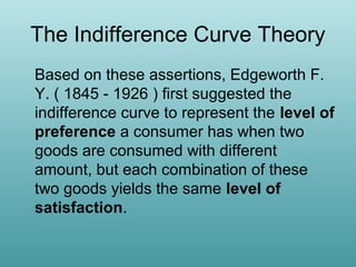
  • 18. Indifference curves are convex [the slopes of IC’s fall as we move from left to right, or we have a diminishing marginal rate of substitution (MRS)] clothing A B C D foo d When we have lots of clothing & not much food (as near A & B), we are willing to give up a lot of clothing to get a little more food. When we have lots of food & not much clothing (as near C & D), we are willing to give up very little clothing to get a little more food.
  • 19. Odd special cases that are not consistent with the properties of Indifference curve listed previously.
  • 20. Perfect Complements tyres IC2 8 IC1 4 1 2 Car bodies You need exactly 4 tyres with 1 car body (ignoring the spare tyre). Having more than 4 tyres with 1 car body doesn’t increase utility. Also having more than 1 car body with only 4 tyres doesn’t increase utility either.
  • 21. Perfect Substitutes Minipacks 10 5 IC1 1 IC2 2 Jumb o pack s Consider two packs of paper; the mini-pack has 100 sheets & the jumbo pack has 500 sheets. No matter how many mini-packs or jumbo packs you have, you are always willing to trade 5 mini-packs for 1 jumbo pack. Since the rate at which you’re willing to trade is the slope of the IC, and that rate is constant, your IC’s have a constant slope. That means they are straight lines.
  • 22. “Neutral” Good Neutral good IC1 IC3 IC2 Your utility is unaffected by consumption of a neutral good. Desire d good
  • 23. The Marginal Rate of Substitution • Def: The MRS of Xof Y refers to the amount of Y that must be given up per unit of X gained by the consumer to keep the level if satisfaction unchanged. • MRSxy= y/ x, where • MRSxy = the MRs of X for Y • Y = a small change in the quantity of Y • X = a small change in the quantity of X
  • 24. The slope of the indifference curve is the rate at which you are willing to trade off one good to get another good. It is called the marginal rate of substitution or MRS.
  • 25. What is the MRS or slope of the IC? points A & B are on the same Suppose Clothing C indifference curve & therefore have the same utility level. IC2 Let’s break up the move from A to B IC1 into 2 parts. A A→D: ∆TU = ∆C (MUC) D→B: ∆TU = ∆F (MUF) B A→B: D 0 = ∆TU = ∆C (MUC) + ∆F (MUF) ⇒ ∆C (MUC) = – ∆F (MUF) ⇒ ∆C/∆F = – MUF / MUC Food F So along an indifference curve, the slope or MRS is the negative of the ratio of the marginal utilities (with the MU of the good on the horizontal axis in the numerator). MRS = – MUX / MUY
  • 26. For example, Clothing C IC1 =90 IC2 = 96 A 6 5 D 7 Suppose IC1 is the 90-util indifference curve & IC2 is the 96-util indifference curve. Point A is 7 units of food & 6 of clothing. B is 9 units of food & 5 of clothing. Since an additional unit of clothing gives you 6 more utils of satisfaction, the MU of clothing must be 6. B Since an additional 2 units of food also give you 6 more utils of satisfaction, the MU of food must be 9Food F 3. So, MRS = – MUF / MUC = -3/6 = -0.5 . You’d give up 2 units of food to get 1 units of clothing.
  • 27. •Hicks replaces the law of DMU by the principle of Diminishing Marginal Rate of Substitution. •As the consumer increases the quantity of X then its MU decreases and % of substitution will be less as the point moves downwards on the IC curve Comm Y Comm X MRS = y / x 10 25 - 11 20 -5/1=-5 12 16 -4/1=-4 13 13 -3/1=-3 14 11 -2/1=-2
  • 28. Budget Constraint Or Budget Line or Price Line • DEF: The Budget line is the locus of points representing all the different combinations of the two goods that can be purchased by the consumer, given his money income and the prices of the two goods. • What a consumer can actually buy depends on the income at his disposal and the prices of goods he wants to buy. • Income and Price are 2 objective factors which form the budgetary constraint of the consumer. • The consumption or purchase possibility of the consumer is restricted to the budget constraint.
  • 29. Contd… • The slope of the budget line is called the marginal rate of substitution in exchange = PX / PY. • The concept of relative price is important because a rise in relative price would encourage the producer to put more resources in production. The concept also conveys the market information of relative scarcity of those resources. • The budget line rotates when the relative price changes. • The shift of the line means that either the income changes or there is a change in the price of both goods.
  • 30. Alternate Purchase Possibilities Given income = Rs. 50 If P of Y = Rs 10/ unit If P of X = Rs 5/ unit AB= Budget ( Price, Income) Line Units of Y Qt of Y a b c s B O Qt of x B X 4 6 1 z 2 2 A 0 3 Y 5 4 A Units of X 8 0 10
  • 31. Budget Constraint or Budget Line This equation tells you what you can buy. For example, suppose you have $24, & there are two goods. The price of the first good is $3 per unit & the price of the second good is $4 per unit. So, if you buy X units of the first good for $3 each, you spend 3X on that good. Similarly, if you buy Y units of the second good, you spend 4Y on that good. Your total spending is 3X+4Y. If you spend all 24 dollars that you have, 3X+4Y=24. That equation is your budget constraint.
  • 32. Example: Budget constraint for $24 of income, and $3 & $4 for the prices of the two goods. Y (0, 6) 0 If you spent all $24 on the 1st good, you could buy 8 units. If you spent all $24 on the 2nd good, you could buy 6 units. So we have the intercepts of the budget constraint. The slope of the line connecting these two points is ∆Y/∆X = – 6/8 = – 3/4 = – 0.75 . (8,0 ) X
  • 33. Let’s generalize. Keep in mind that income was $24 and the prices of the goods were $3 & $4. The equation of the budget constraint in our example was 3X + 4Y = 24. So the budget constraint is p1X + p2Y = I Solving for Y in terms of X, p2Y = I – p1X, or Y = I /p2 – (p1/p2)X Y (0, 6) 0 So from our slope-intercept form, we see that the intercept is I /p2, and the slope is –p1/p2 . The intercept is income divided by the price of the good on the vertical axis. The slope is the negative of the ratio of the prices, with the price of the good on the horizontal axis in the numerator. (8,0 ) X
  • 34. We have the intercept I /p2, & the slope is –p1/p2 . Y (0, 9) (0, 6) 0 What if income increased? The slope would stay the same & the budget constraint would shift out parallel to the original one. Suppose in our example with income of 24 & prices of 3 & 4, income increased to 36. Our new y-intercept will be 36/4 =9 & the new X-intercept will be 36/3=12. (8,0 (12,0 ) ) X
  • 35. Suppose the price of the good on the X-axis increased. Y (0, 6) 0 If we bought only the good whose price increased, we could afford less of it. If we bought only the other good, our purchases would be unchanged. So the budget constraint would pivot inward about the Y-intercept. For example, if the price increased from $3 to $4, our $24 would only buy 6 units. (6,0) (8,0 ) X
  • 36. Similarly, if the price of the good on the Yaxis increased, the budget constraint would pivot in about the X-intercept. Y (0, 6) (0,4) 0 Suppose the price of the 2nd good increased from $4 to $6. If you bought only that good, with your $24, your $24 would only buy 4 units of it. (8,0 ) X
  • 37. Y Y A3 Changes in Income. A2 Px, Py constant A1 Comm of Y Comm of Y A1 O Changes in Price of X B1 B2 B3 X Comm of X O B1 B2 B3 Comm of X A2 Changes in Price of Y Comm of Y A1 Changes in money income, Prices and the BL O X Comm of X B
  • 38. Let’s combine our indifference curves & budget constraint to determine our utility maximizing point. Y IC1 IC2 IC3 Point A doesn’t maximize our utility & it doesn’t spend all our income. (It’s below the budget constraint.) A 0 X
  • 39. Y IC1 IC2 IC3 Points B & C spend all our income but they don’t maximize our utility. We can reach a higher indifference curve. B C 0 X
  • 40. Point D is unattainable. We can’t reach it with our budget. Y IC1 IC2 IC3 D 0 X
  • 41. Y IC1 IC2 Point E is our utility-maximizing point. We can’t do any better than at E. Notice that our utility is maximized at the point of tangency between the budget constraint & the indifference curve. IC3 E 0 X
  • 42. Assumptions of the Consumer Equilibrium • Consumer • • • • Has fixed amount of money income. Intends to buy combination of 2 goods, X and Y. Has definite tastes and preferences. Hence has definite scale of preferences. Expressed through ICM. • S of P remains same through out the analysis. • Is rational and mazimizes his satisfaction • Each of the goods X and Y is homogenous (identical characteristics) and divisible, so various combinations of these goods can be sold.
  • 43. The consumer Equilibrium Qt. of comm Y  Point e is the a M e b N Qt. of comm X equilibrium point given the Budget line.  Satisfaction is max when the MRS of x for y is just equal to the price of x to the price of y.
  • 44. Consumer Optimum or Equilibrium • In mathematics, the slopes of the indifference curve and the budget line are the same. • Slope of the budget line = M R S in exchange = PX / PY • Slope of the indifference curve = M R S in consumption = ∆Y/∆X • In equilibrium, PX / PY = ∆ Y / ∆ X
  • 45. What happens to consumption when income rises? For normal goods, consumption increases. For inferior goods, consumption decreases. What does this look like on our graph?
  • 46. Two Normal Goods Y IC2 IC3 IC1 C Y3 Y2 B As income increases, the budget constraint shifts out & we are able to reach higher & higher IC’s. The points of tangency are at higher & higher levels of consumption of both goods. A Y1 X1 X2 X3 X
  • 47. Income-Consumption Curve Y IC2 IC3 IC1 C Y3 Y2 B The curve that traces out these points is called the income-consumption curve. For two normal goods, the curve slopes upward. It may be convex (as drawn here), concave, or linear. A Y1 X1 X2 X3 X
  • 48. We can also look at consumption levels of two goods when the price of one of them changes. Y Suppose there is an increase in the price of the 1st good (the good on the X-axis). The budget constraint pivots inward. Here we see X drop & Y increase. In this case, our 2 goods are substitutes. Y3 Y2 Y1 X3 X1 X2 X
  • 49. If we connect the points, we have the price consumption curve. It shows the utility-maximizing points when the price of a good changes. Y Y3 Y2 Y1 X3 X1 X2 X
  • 50. If we look at the price of a good & the amount of it consumed, we have the demand curve for our particular individual. P As the price decreases the quantity demanded increases & vice versa. P1 P2 P3 X1 X2 X3 X
  • 51. We can separate the effect of a change in the price of a good on its consumption level into two parts: the income effect & the substitution effect. Y YB YA B XB XA A Suppose the price of the first good increases. The budget constraint was originally the blue line and we were at A consuming quantities XA & YA. After the price change, the budget constraint is the red line, and we’re at B consuming XB & YB . X
  • 52. We first want to capture the effect of the price change without the effect of the change in income. Y H YH YB YA B XB XH XA A We draw a line parallel to the new budget constraint and tangent to the old indifference curve. This will reflect the new relative prices, but since we are tangent to the old indifference curve we are just as well off as initially. Under those circumstances we would be at point H (for hypothetical). Since the 1st good is now relatively more expensive compared to the 2nd, we will substitute, increasing Y & decreasing X. X
  • 53. The movement from A to H is the substitution effect. As a result of the increase in the relative price of the 1st good, we reduce our consumption of it and consume more of the other good. Y H YH YB YA B XB XH XA A X
  • 54. Now we move from H to B Y H YH YB YA B XB XH XA A Our purchasing power has been reduced by the price change. That results in the income effect. In our graph, we now hold the relative prices constant at the new level, but income has fallen. Our budget constraint has shifted inward. If both goods are normal, as a result of the change in income, we reduce our consumption of both goods, and X & Y fall. This is the income effect of the price change. X
  • 55. Total Effect of Price Increase The total effect is to move from A to B. X has fallen. Both the substitution & income effects led to a drop in X. Y has increased in this case. The substitution effect increased consumption of the 2nd good, but the income effect reduced it by less than the substitution effect increased it. Y H YH YB YA B XB XH XA A X
  • 56. Let’s do a price decrease. Y B YB YA A The budget constraint moves from the blue line to the red line. We draw a line parallel to the new budget constraint and tangent to the old indifference curve. H is the tangency of the hypothetical budget constraint with the old indifference curve. The substitution effect is the movement from A to H. We substitute increasing X & decreasing Y. H YH XA XH XB X
  • 57. The movement from H to B is the income effect. As a result of the higher income (greater purchasing power), we consume more of both goods, if they are normal goods. Y B YB YA A H YH XA XH XB X
  • 58. Total Effect The total effect is to move from A to B. X has increased. Both the substitution & income effects led to an increase in X. Y has also increased in this case. The substitution effect decreased consumption of the 2nd good, but the income effect increased it by more than the substitution effect decreased it. Y B YB YA A H YH XA XH XB X
  • 59. Income and Substitution Effects, in words The income effect is the result of the change in purchasing power. If the price of a normal good increases, you feel poorer, and the income effect is to consume less. If the price of a normal good decreases, you feel richer, and the income effect is to consume more. The substitution effect is the result of a change in relative prices. If the price of a good increases, the substitution effect is to consume less of it & more of the other goods that are now relatively cheaper. If the price decreases, the substitution effect is to consume more of it & less of the goods that are now relatively more expensive.