PART II.2 - Modern Physics
1 like1,010 views

This document discusses the incompatibility between classical mechanics and electromagnetism. It shows that under a Galilean transformation, the wave equation governing electromagnetic waves takes on a different form in different reference frames, violating Galilean invariance. This means that the laws of electromagnetism depend on the choice of reference frame. As such, classical mechanics and electromagnetism cannot be unified without modifications to account for this issue.


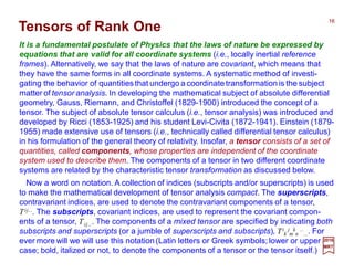
![The acceleration of a particle is the time derivative of its velocity (i.e., ax =dux /dt, &c).
To find the Galilean acceleration transformations we differentiate the velocity transfor-
mations above (using the fact that t=t and v is considered a constant) to obtain:
The relationship between [ux,uy,uz] and [ux,uy,uz] is obtained from the time differen-
tiation of the Galilean coordinate transformation x ↔x. Thus, from r=x i and x =x −vt:
vuv
td
xd
td
td
td
vtxd
td
vtxd
td
xd
u xx −=
−=
−
=
−
== )1(
)()(
2017
MRT
where −v is the velocity of frame S relative to S. Altogether, the Galilean velocity transfor-
mations are:
zzyyxx uuuuvuu ==−= and,
zzyyxx aaaaaa === and,
Thus the measured acceleration components are the same for all observers moving with
uniform relative velocity. (N.B., That is why v was chosen to be a constant since it gives
us a uniform relativistic motion to deal with otherwise things get really complicated).
8
ˆ
In addition to the coordinate of an event, the velocity of a particle is of interest. Two ob-
servers, O and O, will describe the particle’s velocity by assigning three components to it,
with [ux,uy,uz] being the velocity components as measured by O in frame S and [ux,uy,uz]
being the velocity components as measured by O (i.e., relative to frame S).](https://image.slidesharecdn.com/2-170115192041/85/PART-II-2-Modern-Physics-8-320.jpg)
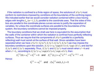
![Since, in elementary mechanics, longitudinal sound waves and transverse waves
along a string are familiar phenomena, one might expect that electromagnetic waves
should obey the same laws that govern such mechanical waves. Such a situation would
be very desirable, for then the physics of electromagnetism might be unified
conceptually with the physics of massive bodies. Let us therefore test the applicability of
classical mechanics to electromagnetic theory by carrying out a Galilean transformation
on the wave equation governing electromagnetic waves.
9
2017
MRT
We are interested in the telegrapher’s equation:
0),(
1
2
2
2
2
=
∂
∂
−∇ tf
tc
r
where f (r,t) is a scalar function of r ≡ri and t. Now, under a Galilean transformations,ri
→ri =ri −vit, and since f (r,t) is a scalar function, it must have the same numerical value
in both coordinate systems, although its form as a function of r and t may be different.
Thus, let:
]),,([),(),( ttgtgtf rrrr ==
where the last member demonstrates that g depends of t implicitly through the
dependence of r(r,t) on t, as well as explicitly.](https://image.slidesharecdn.com/2-170115192041/85/PART-II-2-Modern-Physics-9-320.jpg)
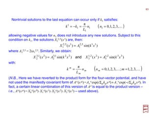
![Now we have:
10
2017
MRT
jj j
jj
k k
jk
k kj
k
j r
tg
r
tg
r
tg
r
tg
r
r
r
tf
∂
∂
=
∂
∂
=
∂
∂
=
∂
∂
∂
∂
=
∂
∂
∑∑∑=
),(),(),(),(),(
3
1
rrrrr
δδ
since δk j =∂rk /∂rj has the definition δkj =1 when k= j and δkj =0 when k≠ j, so that:
),(),( 22
tgtf rr ∇=∇
However:
t
tg
tg
t
tg
r
tg
t
r
t
tf
k k
k
∂
∂
+•=
∂
∂
+
∂
∂
∂
∂
=
∂
∂
∑=
),(
),(
),(),(),(
3
1
r
rv
rrr
∇∇∇∇
and:
444444 3444444 21
incouplingordersecondandFirst ∇∇∇∇
∇∇∇∇∇∇∇∇∇∇∇∇
•
••+
∂
∂
•+
∂
∂
=
∂
∂
v
rvv
r
v
rr
)],([
),(
2
),(),(
2
2
2
2
tg
t
tg
t
tg
t
tf
Therefore, the telegrapher’s equation transforms Galileanly according to the rule:
0),(
1
2),(
1
2
2
22
2
2
2
2
2
=
∂
∂
−
∂
∂
•−
•
•−∇=
∂
∂
−∇ tg
tctccc
tf
tc
r
vvv
r ∇∇∇∇∇∇∇∇∇∇∇∇
or
0),()()(2
1
),(
1 2
2
2
2
2
2
2
2
2
=
•+
∂
∂
•+
∂
∂
−∇=
∂
∂
−∇ tg
ttc
tf
tc
rvvr ∇∇∇∇∇∇∇∇
Yikes!](https://image.slidesharecdn.com/2-170115192041/85/PART-II-2-Modern-Physics-10-320.jpg)

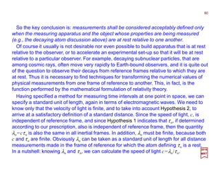
![According to Coulomb’s law, fC(r)= (1/4πεo)ρ(r)∫∫∫V ρ(r)[(r−−−−r)/|r−−−−r|3]d3r, and the law of
Biot and Savart, fBS(r)= (µo/4π)J(r)××××∫∫∫V J(r)××××[(r−−−−r)/|r−−−−r|3]d3r, the total force f(r) per unit
volume exerted on a charge density ρ(r) and current density J(r) is:
12
2017
MRT
)()()()()()()( BSC rBrJrErrfrfrf ××××++++++++ ρ==
Now if the charge density vanishes everywhere except at a single point ro, and is so
large at ro that ∫∫∫V ρ(r)d3r=q is a finite number (if ro is in V of course), then we can write:
ˆ
)()( orrr −−−−δρ q=
that is, we have a point charge of magnitude q at ro. Similarly, if J(r) is generated by a
point charge of magnitude q moving with velocity v(r), have:
)()()()()( oo rrrvrvrrJ −−−−δρ q==
when the charge is at ro.
)]()([)()]()([
)]()()()([)(
ooo
33
rBrrrvrErr
rrBrJrErrrfF
××××−−−−++++−−−−
××××++++
δδ
ρ
qq
dd
VV
=
== ∫∫∫∫∫∫
so that we obtain:
)]()()([ ooo rBrvrEF ××××++++q=
With these expressions for the charge and current densities,the total force experienced
by the charge evidently is:
This is the Lorentz force law, which is in this case, as seen from an origin O, ro away.](https://image.slidesharecdn.com/2-170115192041/85/PART-II-2-Modern-Physics-12-320.jpg)
![The field vectors E(r) and B(r) can be written in terms of the scalar and vector
potentials, according to E(r)= −∇∇∇∇φ(r)−−−−∂A(r)/∂t and B(r)= ∇∇∇∇××××A(r), and for fields gene-
rated by a point charge q at r, the potentials given by φ(r)=(1/4πεo)∫∫∫V ρ(r)(1/|r−−−−r|)d3r
and A(r)=(µo/4π)∫∫∫V J(r)(1/|r−−−−r|)d3r] become:
13
2017
MRT
rr
rv
rA
rr
r
−−−−−−−−
)(
π4
µ
)(
1
επ4
)( o
o
qq
== andφ
where v(r) is the velocity of the source charge q. If the velocity v(r) is a constant, we
then have:
)(
π4
µ
)(
)(
επ4
)( 3
o
3
o
rv
rr
rr
rA0
rA
rr
rr
r ××××
−−−−
−−−−
××××∇∇∇∇
−−−−
−−−−
∇∇∇∇
q
t
q
−==
∂
∂
=− and,φ
Therefore the fields at point r arising from a uniformly moving charge q at r are:
3
o
3
o
)()(
π4
µ
)(
επ4
)(
rr
rrrv
rB
rr
rr
rE
−−−−
−−−−××××
−−−−
−−−− qq
== and
The force on charge q at ro due to these fields is:
)]}()([)(εµ){(
1
επ4
)]()()([ ooooo3
oo
ooo rrrvrvrr
rr
rBrvrEF −−−−××××××××++++−−−−
−−−−
××××++++
qq
q ==
where the first term is the electromagnetic force and the second is the magnetic
force. This is familiar from elementary physics of point charges.](https://image.slidesharecdn.com/2-170115192041/85/PART-II-2-Modern-Physics-13-320.jpg)
]}()([)({)(
π4
µ
)( ooo3
o
o
o rrrvrvrr
rr
Frr −−−−××××××××××××−−−−
−−−−
××××−−−−ττττ
qq
==
Consider the arrangement shown in the Figure, for which we take v(r)=v(ro)=v. Here
we have:
Schematic diagram of the arrangement of the
Trauton-Noble experiment.
If the angle between v and r is θ, the multiple cross-pro-
duct on the right-hand side can be rewritten in terms of θ as:
where r××××v ≡(r××××v)/|r××××v| is a unit vector in the direction of r××××v.
Hence the torque tending to restore the vector r to an
orientation perpendicular to v is (N.B., we use c2 =1/µoεo):
2017
MRT
where r=ro −−−−r.
vr
vr
vrrvrvrvrrvvr
××××
××××
××××−−−−××××××××××××××××
ˆ2sin
2
1
ˆcossin
))((])[()]([
22
22
2
θ
θθ
rv
rv
v
=
=
•=•=
ˆ
vr ××××ττττ ˆ2sin
επ4
1
2
o
θ
=
c
v
r
qq
v
r
v
q
Pivot
q
_
ro
r
O
v××××(v×××× r)
r××××vˆ
θ
2
π
θ −
2
π
ττττ](https://image.slidesharecdn.com/2-170115192041/85/PART-II-2-Modern-Physics-14-320.jpg)

![defines a new coordinate system specified by the mutually independent variables: x1, x2,
…, xn. The symbol φ i (e.g., a temperature distribution or field of some sort) are ass-
umed to be single-valuedreal functions of the coordinates with continuous derivatives.
The rank (order) of a tensor is the number (without counting an index which appears
once as a subscript and once as a superscript) of indices in the letter or symbol
representing a tensor (or the components of a tensor). Here a few examples of tensor
(and their rank) which will make an appearance very soon: S is a tensor of rank zero
(scalar – e.g., action); xi is a covariant vector of rank one (covariant vector – e.g., three-
dimensional Cartesian coordinate); Pµ is a contravariant tensor of rank one (contra-
variant vector – e.g., space-time momentum); Tµ
ν is a mixed tensor of rank two (e.g.,
energy-momentum-stress tensor) ; Gµν =Rµν +½gµνR is a (contravariant–e.g., Einstein’s
gravitational field tensor) tensor of rank two; Rµν ≡Σλ Rλ
µλν (note the contraction on the
index λ) is a tensor (e.g., Ricci curvature tensor) of rank two; Rµ
νρσ is a mixed tensor
(e.g., action Riemann curvature tensor) of rank four; and finally R ≡ΣµΣν gµν Rµν (i.e.,
another contrac-tion on both µ andν) is a tensor of rank zero (scalar – e.g., curvature
scalar). In an n-dimensional space, the number of components of a tensor of rank n is nr.
( )nixxxx nii
,,2,1),.,,( 21
KK == φ
Consider a ordered set of n mutually independent real variables x1,x2,…,xn =[xi],
called the coordinate of a point, Pn(x1,x2,…,xn). The collection of all such points
corresponding to all the sets of values [xi] forms an n-dimensional linear space (i.e., a
manifold – French for variété) which we specify by Vn. The set of n equations:
2017
MRT
17](https://image.slidesharecdn.com/2-170115192041/85/PART-II-2-Modern-Physics-17-320.jpg)


![In anisotropic media, the relation between the vector P and E depends on the direction
of the vector E, and these two vectors are not necessarily parallel. If the medium is
linear, nondispersive, and homogeneous, each component of P=[P1,P2, P3] is a linear
combination of the three components of E=[E1,E2, E3]:
2017
MRT
24
=
++++++++=
++== ∑=
3
2
1
332313
322212
312111
o
333o223o113o332o222o112o331o221o111o
33o22o11o
3
1
o
ε
εεεεεεεεε
εεεε
E
E
E
EEEEEEEEE
EEEEP iii
j
jjii
χχχ
χχχ
χχχ
χχχχχχχχχ
χχχχ
where the indices i, j =1,2,3 denote the x, y, and z components. The dielectric properties
of the medium are described by an array [χij] of 3×3 constants known as the
susceptibility tensor.
Also for anisotropic media, a similar relation as above between D and E applies:
where [εij] are elements of the electric permittivity tensor.
== ∑=
3
2
1
332313
322212
3121113
1 εεε
εεε
εεε
ε
E
E
E
ED
j
jjii](https://image.slidesharecdn.com/2-170115192041/85/PART-II-2-Modern-Physics-24-320.jpg)

![We began our discussion of special relativity by demonstrating that the demands of
Maxwell’s theory of electromagnetism were not consistent with the hypotheses of
Newtonian mechanics. Einstein (with Minkowski’s help) has shown us how to
reformulate physics, in terms of a rather elegant four-dimensional mathematical
framework, such that the two classical theories could be welded together into a unified
structure. We will now work out Maxwell’s theory into the same four-dimensional
framework. That this reformulation of electromagnetism will yield rather elegant and
apparently simple equations should be a gratifying reward for our efforts.
26
2017
MRT
vJ ρ=
In our original expression for the current density vector we had:
where ρ is the charge density for a distribution of charge moving with velocity v relative
to an observer. This suggests that the four-vector representation for the current density
might be:
τ
ρρ
µ
µµ
d
xd
uJ ==
where ρ is the invariant charge density (i.e., the charge density as seen by an observer
at rest relative to the charge involved). The components of the current density four-
vector are given by:
],[ vργργµ
cJ =
which is obtained by letting dτ =(1/γ )dt with γ =1/√(1−v2/c2) and using v=dx/dt.](https://image.slidesharecdn.com/2-170115192041/85/PART-II-2-Modern-Physics-26-320.jpg)
![This discussion immediately yields an interpretation for the temporal component of J µ.
Evidently, J 0 =γ ρc is just c times the charge density as seen by an observer relative to
whom the charges are moving with velocity v (i.e., J 0 is c times the charge density of the
charges having current density J=γ ρv). In the limit v/c<<1, we have γ ≅1, and:
27
2017
MRT
vJ ρρ ≅≅ andcJ 0
as the nonrelativistic approximations for the components of the current density four-
vector.
A particular pleasant result of this formulation of a four-vector current density is that the
equation of continuity takes a very simple form, namely:
03
3
2
2
1
1
0
0
3
0
=∂+∂+∂+∂=∂=
∂
∂
∑∑=
JJJJJ
x
J
µ
µ
µ
µ
µ
µ
and which, otherwise, would be written as:
0)(
)(1
=•+
∂
∂
vργ
ργ
∇∇∇∇
t
c
c
],,,[],[],,,[ 3210
zyxctctxxxxx ===≡ rµ
x
where we have set the following Cartesian coordinates to simplify things:](https://image.slidesharecdn.com/2-170115192041/85/PART-II-2-Modern-Physics-27-320.jpg)


![In matrix notation, we then have:
33
2017
MRT
Note that the third matrix on the right hand side of the equation is the transpose of
the first (i.e., the matrix formed by interchanging rows and columns so that the
element in the µ-th row and ν -th column of the original matrix appears in the ν -th
row and µ-th column of the transpose matrix).
ΛΛΛΛ
ΛΛΛΛ
ΛΛΛΛ
ΛΛΛΛ
ΛΛΛΛ
ΛΛΛΛ
ΛΛΛΛ
ΛΛΛΛ
=
ΛΛΛΛ
ΛΛΛΛ
ΛΛΛΛ
ΛΛΛΛ
ΛΛΛΛ
ΛΛΛΛ
ΛΛΛΛ
ΛΛΛΛ
=
ΛΛ=
= ∑ ∑= =
3
3
3
2
3
1
3
0
2
3
2
2
2
1
2
0
1
3
1
2
1
1
1
0
0
3
0
2
0
1
0
0
33323130
23222120
13121110
03020100
3
3
3
2
3
1
3
0
2
3
2
2
2
1
2
0
1
3
1
2
1
1
1
0
0
3
0
2
0
1
0
0
3
3
3
2
3
1
3
0
2
3
2
2
2
1
2
0
1
3
1
2
1
1
1
0
0
3
0
2
0
1
0
0
33323130
23222120
13121110
03020100
3
3
3
2
3
1
3
0
2
3
2
2
2
1
2
0
1
3
1
2
1
1
1
0
0
3
0
2
0
1
0
0
3
0
3
0
33323130
23222120
13121110
03020100
][][][
FFFF
FFFF
FFFF
FFFF
FFFF
FFFF
FFFF
FFFF
F
FFFF
FFFF
FFFF
FFFF
F
T
T
µ ν
σ
ν
νµρ
µ
σρ](https://image.slidesharecdn.com/2-170115192041/85/PART-II-2-Modern-Physics-33-320.jpg)


![Hence, according to our interpretation of −T0
0 as the energy density E of the field, we
have:
48
2017
MRT
We have ignored most of the components of Tµ
ν . Since the previous matrix
representing Tµ
ν is symmetric in its indices (i.e., Tµ
ν =Tν
µ), there are only 10, rather than
16, independent components of the tensor. We have discussed four of these
components; the other six define the so-called Maxwell stress-energy tensor, which is a
tensor under three-dimensional rotations. These do not play any important role in our
discussion of the four-dimensional formulation of electromagnetic theory, and we will not
consider them further.
+=−= 2
o
2
o
0
0
µ
1
ε
2
1
BETE
here we have used the relationship 1/c2 =εoµo. Furthermore, since −(1/c)T i
0, for i=1,2,3,
are the components of the momentum density P, we also have the result:
BE××××oε=P
Sometimes one writes P =(1/c2)[E××××(1/µo)B], and [E××××(1/µo)B] is called the Poynting
vector. It is important to note that the energy and momentum densities, E and P, are not
components of a four-vector, but rather are components of a tensor (i.e., the energy-
momentum – in this case mixed – tensor Tν
µ) of rank two, just as E and B are not
components of four-vectors but rather are components of rank-two tensors.](https://image.slidesharecdn.com/2-170115192041/85/PART-II-2-Modern-Physics-48-320.jpg)


![The solution for X1
ν then can be written in the form:
52
2017
MRT
0)()()()( 220
3
1
220
=−=− ∑=
kkkk
i
i
Similarly, by continuing these arguments, we obtain:
1111
ee)( 11
1
1
xkixki
baxX −
+= ννν
33332222
ee)(ee)( 33
3
322
2
2
xkixkixkixki
baxXbaxX −−
+=+= νννννν
and
where k0, k1, k2, and k3 must satisfy:
This last equation must be satisfied in all coordinate frames because the equation that
we are solving (i.e., Σµ∂µ∂µ Aν =0) is relativistically covariant (i.e., it is valid in every
inertial frame of reference). Therefore (k0)2 −(k)2 must be an invariant quantity, and since
it has the form of the inner product of two four-vectors, we conclude that:
],[],,,[ 03210
kkkkkkk ==µ
is a contravariant four-vector. Similarly:
],[ 0
k−== ∑ kkk
ν
ν
νµµ η
is a covariant four-vector and ηµν is the metric.](https://image.slidesharecdn.com/2-170115192041/85/PART-II-2-Modern-Physics-52-320.jpg)


![Finally, let the amplitude of a light wave of frequency ν and wavelength λ be
represented by Acos(ωt−k•x), where ω=2πν and k=(2π/λ)k, k being the direction of
propagation of the wave. Since, according to special relativity, light travels with the same
speed in all inertial frames of reference, ωt−k•x must be an invariant under Lorentz
transformations:
55
2017
MRT
xkxk •−=•− tt ωω
where the bared quantities are in the S-frame moving with velocity v (along the z-axis,
say) relative to S. This suggests that we define:
ˆˆ
== kk ,
ω
],[ 0
c
kk µ
so that:
xk •−=∑ tkk ω
µ
µ
µ
as seen above so from the fact that Σµkµkµ is an invariant we can show that kµ is a true
four-vector.](https://image.slidesharecdn.com/2-170115192041/85/PART-II-2-Modern-Physics-55-320.jpg)


![We find, therefore, that only the first term on the right-hand side of our result for Tν
µ
survives; that is:
60
2017
MRT
whenever Aλ represents a solution to the inhomogeneous wave equation. From this we
find (recall the energy density of the field, E =½[εoE2+(1/µo)B2]):
∑ ∂∂=
λ
λµ
λνν
µ ))((
µ
1
o
AAT
∑ ∂∂−=−=
λ
λ
λ
))((
µ
1
0
0
o
0
0 AATE
and for i=1,2,3:
E
P
k
k
i
iii
xkixkixkixkii
ii
k
c
T
k
c
T
k
k
c
AA
k
k
c
AAAAkk
c
AA
c
T
c
1
11
))((
µ
1
eeee)(
µ
1
))((
µ
11
0
0
0
0
0
0
0
0o
0
o
0
o
0
=
==∂∂=
−
−−=
∂∂−=−=
∑
∑
∑∑∑∑ −
−+
−
−+
λ
λ
λ
λλ
λλ
λ
λ
λ
σ
σ
σσ
σ
σρ
ρ
ρρ
ρ
ρ](https://image.slidesharecdn.com/2-170115192041/85/PART-II-2-Modern-Physics-60-320.jpg)
![Writing this last result in three-vector form, we have:
61
2017
MRT
that is, the momentum density, P, of the wave field is in the direction of advancing
wavefronts, k=k/|k|, and its magnitude is equal to 1/c time the energy density, E.
k
k
k ˆ11
EEP
cc
==
ˆ
Comparing P =εoE××××B derived previously P =(1/c)(k/|k|)E above, we observe that E××××B
also is in the direction of k, and that:
+
=
+
=
+⋅== 2
2
2
2
oo
2
o
2
o
oo
1
2
1
ε2
11
ε
2
1
ε
1
ε
1
BEBEBEBE
c
c
cccc µµ
E××××
where we made use of E =½[εoE2+(1/µo)B2] again. This result can be written in the form:
which implies that |E××××B|=|E||B| so that E is perpendicular to B, and also that (1/c)|E|=|B|.
0
1
2
1 2
2
=+−
BBEE ××××
cc
In summary, k, E, and B, in that order or in any cyclic permutation of that order, form a
right-handed system of orthogonal vectors, and the magnitude of E is equal to c times
the magnitude of B; the energy density of the electromagnetic radiation field therefore is
E =εoE2. These are classical results for wave fields, and may be recalled from
elementary physics courses; here we have seen how they emerge from the four-
dimensional formalism.](https://image.slidesharecdn.com/2-170115192041/85/PART-II-2-Modern-Physics-61-320.jpg)


![In June 1905, in a paper entitled On the Electrodynamics of Moving Bodies, Einstein
introduced the special theory of relativity. Here is the opening passage:
2017
MRT
“It is known that Maxwell’s electrodynamics – as usually understood at
the present time – when applied to moving bodies, leads to asymmetries
which do not appear to be inherent in the phenomena. Take for example,
the reciprocal electrodynamic action of a magnet and a conductor. The
observable phenomenon here depends only on the relative motion of
the conductor and the magnet, whereas the customary view draws a
sharp distinction between the two cases in which either the one, of the
other of the bodies, is in motion. Examples of this sort, together with the
unsuccessful attempts to discover any motion of the Earth relative to
the ‘light medium,’ [n.d.l.r., the ‘ether’] suggest that the phenomenon of
electrodynamics as well as of mechanics possess no properties
corresponding to the idea of absolute rest.” (A. Einstein, Annalen der
Physik, 17, 891 (1905))
70](https://image.slidesharecdn.com/2-170115192041/85/PART-II-2-Modern-Physics-70-320.jpg)


![If we were dealing with the current-density vector J with components Jx, Jy, and Jz, we
would have obtained the following result:
75
2017
MRT
with of course, u2 =ux
2 +uy
2 +uz
2. There is an important significance in the equation ρ =
ρo/√(1−u2/c2)… Just as c2t2 −(x2 +y2 +z2) is equal to an invariant quantity c2τ 2, and m2c2 −
(px
2 +py
2 +pz
2) is equal to an invariant quantity mo
2c2; similarly, we can treat p2c2 −(Jx
2 +Jy
2 +
Jz
2) as an invariant quantity equal to ρo
2c2. This means that J and ρ transform exactly like
p and m, and hence if in a general case, S is moving with a velocity v along the x- and x-
axes, the quantities [ρ, Jx , Jy , Jz ] and [ρ, Jx , Jy , Jz ] are related by the transformation
equations:
2
2
o
2
2
o
2
2
o
2
2
o
1111
c
u
u
J
c
u
u
J
c
u
u
J
c
u
z
z
y
y
x
x
−
=
−
=
−
=
−
=
ρρρρ
ρ &,and
zzyy
x
xzzyy
x
x
xx
JJJJ
c
v
vJ
JJJJJ
c
v
vJ
J
c
v
J
c
v
c
v
J
c
v
SSSS
==
−
+
===
−
−
=
−
+
=
−
−
=
&,&,
toFromtoFrom
2
2
2
2
2
2
2
2
2
2
11
11
ρρ
ρ
ρ
ρ
ρ](https://image.slidesharecdn.com/2-170115192041/85/PART-II-2-Modern-Physics-75-320.jpg)


![We now need to connect measurements made by an observer O along coordinate axes
in frame S with those of another observer O made in S. To do so, we will perform a mathe-
matical derivation that will yield the required transformation equations between frames.
81
2017
MRT
),,,( tzyxxx =
Because of the impossibility of synchronizing pairs of clocks in different reference
frames, the time coordinate and the space coordinates cannot be kept completely
separate for observers in different reference frames; the spatial separation between
clocks in one frame of reference makes these clocks seem nonsynchronous in any other
frame. Similarly, if two spatially separated events occur at different times in one frame of
reference, the time interval separating the events in that frame will affect the apparent
spatial separation between them as measured in any other coordinate frame. Thus if x,
y, z, and t are the space and time coordinates in S, we must expect that in a comparison
between the coordinate systems, x may depend on x, y, z, and t:
and similarly:
),,,(),,,(),,,( tzyxtttzyxzztzyxyy === and,
We therefore say that the comparison between coordinate systems may be accom-
plished by a coordinate transformation from [x,y,z,t] to [x,y,z,t], and the transformation is
determined by the functional dependence of the unbared coordinates upon the bared
coordinates (N.B., t is given the same status here as the spatial coordinates x, y, and z,
and also, because of the symmetry between S and S, a transformation in the reverse
direction, from coordinates of S to those of S, must exist viz x=x(x,y,z,t), &c.)](https://image.slidesharecdn.com/2-170115192041/85/PART-II-2-Modern-Physics-81-320.jpg)


![Thus the hypothesis that space and time are homogeneous has led us to the require-
ment that any transformation between coordinates in different frames of reference must
be a linear transformation (i.e., straight lines in one frame are transformed into straight
lines in another) as opposed to second order transformations (i.e., nonlinearities arise).
84
2017
MRT
zyxctzxzyxctyx
zyxctxxzyxcttcx
3
3
3
2
3
1
3
0
32
3
2
2
2
1
2
0
2
1
3
1
2
1
1
1
0
10
3
0
2
0
1
0
0
0
Λ+Λ+Λ+Λ==Λ+Λ+Λ+Λ==
Λ+Λ+Λ+Λ==Λ+Λ+Λ+Λ==
and
,,
To make clear the meaning of the xµ(xν )=Σν Λµ
ν xν equation above, let us write it out
explicitly by expanding the sum over ν =0,1,2,3, using [x0,x1,x2,x3]≡[ct,x,y,z], &c. Thus:
So, the xµ(xν )=Σν Λµ
ν xν and xµ(xν )=Σν Λµ
ν xν equations represent four equations each.
We can combine the xµ(xν )=Σν Λµ
ν xν and xµ(xν )=Σν Λµ
ν xν equations to get:
∑ ∑∑ ∑∑
ΛΛ=
ΛΛ=Λ=
λ
λ
ν
ν
λ
µ
ν
ν λ
λν
λ
µ
ν
ν
νµ
ν
µ
xxxx
Hence, since the magnitude of xµ is arbitrary, we must have:
µ
λ
ν
ν
λ
µ
ν δ=ΛΛ∑
where δ µ
λ=0 if µ ≠λ and δ µ
λ=1 if µ =λ so that, in fact:
µ
λ
λµ
λ
µ
δ xxx == ∑
while recalling that all the sums above run over ν,λ=0,1,2,3.](https://image.slidesharecdn.com/2-170115192041/85/PART-II-2-Modern-Physics-84-320.jpg)
![Now we introduce the hypothesis that the speed of light is independent of reference
frame. Let a light pulse be emitted from a source at point [a1,a2,a3] at time a0/c (i.e., at
the four-point [a0,a1,a2,a3]). After a time (x0/c)−(a0/c) the wave front will have traveled to
the surface of radius x0 −a0, and the equation for this surface is:
85
2017
MRT
00233222211
)()()( axaxaxax −=−+−+−
for x0 >a0, or:
0)()()()( 233222211200
=−−−−−−− axaxaxax
Since the velocity of light is the same in S as in S, the wave front of the pulse will have
reached a sphere of radius x0 −a0 in S after a time (x0 −a0)/c as measured by clocks at
rest in S, where aµ is the four-point in S at which the pulse is emitted. Hence the equation
for this surface is:
0)()()()( 233222211200
=−−−−−−− axaxaxax
the left-hand side of the last two equations above have the same form; hence the
equations for the surface representing the wave front of an electromagnetic wave are
form-invariant (i.e., covariant – the form of the equations is the same in all frames of
reference).
(1)
(2)](https://image.slidesharecdn.com/2-170115192041/85/PART-II-2-Modern-Physics-85-320.jpg)


![Using the fact that c∆τ =√[(∆s)2]=√(Σµ ∆xµ∆xµ) is an invariant, we can construct a
particularly useful four-vector. The velocity of one reference frame relative to another
can be defined in terms of:
98
2017
MRT
τττ d
d xx
u =
∆
∆
=
→∆ 0
lim
where ∆x is a proper measurement of the change of position of the origin of one frame
relative to another in the proper time interval ∆τ. Generalizing this to four dimensions:
ττ
µµ
τ
µ
d
xdx
u =
∆
∆
=
→∆ 0
lim
for the four-velocity of a point stationary in some frame S, as seen by an observer O in S.
Clearly the clock measuring ∆τ must be at rest relative to S, for otherwise two clocks
would be required, one at each endpoint of the spatial interval traversed by the point that
is at rest in S, and the time interval would not be a proper one. On the other hand, ∆xµ
must be measured in S, since the point is a rest in S; thus the proper distance traversed
by the point is to be measured in S whereas the proper time is to be measured in S.
The four-velocity defined in this way is a four-vector, since ∆xµ is a four-vector and ∆τ
is an invariant. Specifically:
∑∑∑ Λ=
∆
∆
Λ=
∆
∆Λ
=
∆
∆
=
→∆→∆→∆
ν
ν
µ
ν
ν
ν
τ
µ
ν
ν
νµ
ν
τ
µ
τ
µ
ττττ d
xdxxx
u
000
limlimlim
since Λµ
ν is independent of space and time intervals.
Relativistic Kinematics](https://image.slidesharecdn.com/2-170115192041/85/PART-II-2-Modern-Physics-98-320.jpg)

![We are now in a position to write uµ in terms of u and v. First:
100
2017
MRT
γ
τττ
c
d
td
c
d
tcd
d
xd
===
)(0
hence:
],[],,,[ uγγµ
cuuucu zyx ==
Since γ appears in this expression, and since it is v=(1/γ )u that one measures in
practice, a more useful expression for uµ is:
],[],[],,,[ vv ccvvvcu zyx γγγγγγγµ
===
Hence, to construct a four-vector from v, one must multiply each component of v by γ =
(1−β 2)−1/2 where β =v/c, and append the zeroth component, γ c. The four-velocity uµ thus
is related to the usual three-dimensional velocity v in a somewhat more complicated way
than xµ is related to x.](https://image.slidesharecdn.com/2-170115192041/85/PART-II-2-Modern-Physics-100-320.jpg)
![An important invariant in physics is the proper mass or rest mass of a particle; as the
name suggests, this invariant is just the mass as measured by an observer at rest
relative to the particle. Typically the is called the mass of the particle but we will highlight
the rest part by a naught: mo.
101
2017
MRT
τ
µ
µµ
d
xd
mump oo ==
Given the invariant mass, mo, of a particle, we can define another important four-
vector, the four-momentum:
for which we have:
∑∑∑ Λ=Λ=Λ==
ν
νµ
ν
ν
νµ
ν
ν
νµ
ν
µµ
pumumump )( ooo
In view of uµ =[γc,γ v] above, we can write:
],[ oo vmcmp γγµ
=](https://image.slidesharecdn.com/2-170115192041/85/PART-II-2-Modern-Physics-101-320.jpg)

![An important property of Lorentz transformations is their group property. Any set A of
objects for which an associative law of combination (i.e., the product ‘⋅’) is defined such
that:
103
2017
MRT
µ
ν
ρ
ρ
ν
µ
ρ ][ bababa ==⋅ ∑
1. If elements a∈A and b∈A belong to a set A, then a⋅b∈A;
2. There exists an identity element e∈A such that for any a∈A, a⋅e=e⋅a=a;
3. For every element a∈A, there exists another element of A, called the inverse a−1,
such that aa−1 =a−1a=e;
is called a mathematical group. If we let A be the set of Lorentz transformations, and if a
≡aµ
ν (e.g., a matrix [a]µ
ν), b≡bµ
ν are elements of that set, with a⋅b defined as:
it is easy to show that A is a group.
Now, to be specific, let {Λµ
ν} (i.e., corresponding to a above) be the set of Lorentz
coefficients for a transformation from frame S to frame S: x µ =Σν Λµ
ν xν, and let {Λµ
ν} (i.e.,
b above) be the set L of Lorentz coefficients for a transformation from frame S to frame S
:x µ =Σν Λµ
ν xν. Then, if the set of coefficients for transforming from S to S, one has:
∑∑∑ ΛΛ=Λ=Λ=
ρν
νρ
ν
µ
ρ
ρ
ρµ
ρ
ν
νµ
ν
µ
xxxx
or, since xν is arbitrary:
Λ⋅Λ=ΛΛ=Λ≡Λ µ
ν
µ
ν ][][
is the transformation from S to S (i.e., Λ=Λ⋅Λ∈L).](https://image.slidesharecdn.com/2-170115192041/85/PART-II-2-Modern-Physics-103-320.jpg)
![Next, let δ µ
ν =1 then Λ⋅1=[Λδ ]µ
ν =[Λ]µ
ν =Λ and 1⋅Λ=[δ Λ]µ
ν =[Λ]µ
ν =Λ. The
transformation 1=[δ ]µ
ν is just the identity transformation (e.g., from S to S); hence 1∈L
(i.e., corresponding to e∈A above) is the identity that is required. Furthermore, let Λ−1 =
[Λ]µ
ν (i.e., Λ−1 is the set of transformation coefficients for S →S). Then:
104
2017
MRT
1][][][ 11
=ΛΛ=ΛΛ==ΛΛ=Λ⋅Λ −− µ
ν
µ
ν
µ
ν δ
and requirement 3 above is satisfied (i.e., if 1 corresponds to e above). Since ordinary
multiplication and addition are associative, we also have, for any Λ,Λ,Λ∈L:
)()]([])[()()( Λ⋅Λ⋅Λ=ΛΛΛ=ΛΛΛ=ΛΛΛ=Λ⋅Λ⋅Λ ∑ µ
σ
µ
σ
ρν
ρ
σ
ν
ρ
µ
ν
so that our law of combinationindeed is associative (i.e., corresponds to (a⋅b)⋅c=a⋅(b⋅c)).
Hence the set L (or equivalently the set A above) is a group, and for this reason the set
of all Lorentz transformations often is referred to as the Lorentz group L.](https://image.slidesharecdn.com/2-170115192041/85/PART-II-2-Modern-Physics-104-320.jpg)
![As an application of the group property among special Lorentz transformations, along
the x-axis, say, we shall find the transformation that carried four-vectors as measured in
S to four-vectors in S, by calculating the result of first transforming from S into some
intermediate frame S, and then transforming from S into S. Thus if:
105
2017
MRT
∑∑∑ Λ=Λ=Λ=
ν
νµ
ν
µ
ν
νµ
ν
µ
ν
νµ
ν
µ
xxxxxx and,
we have:
∑∑∑ ΛΛ=Λ=Λ=
ρν
νρ
ν
µ
ρ
ρ
ρµ
ρ
ν
νµ
ν
µ
xxxx
or since the xν are arbitrary, as above:
∑ ΛΛ=Λ
ρ
ρ
ν
µ
ρ
µ
ν
If vx is the velocity of S relative to S, and if vx is the velocity of S relative to S, we have
the matrices for Λµ
ν and Λµ
ν along the x-axis (using the unit vector x to indicate this):
−
−
=Λ
−
−
=Λ
1000
0100
00
00
][
1000
0100
00
00
][ ˆˆˆ
ˆˆˆ
ˆ
ˆˆˆ
ˆˆˆ
ˆ
xxx
xxx
x
xxx
xxx
x
γβγ
βγγ
γβγ
βγγ
µ
ρ
ρ
ν and
where γx =(1−βx
2)−1/2 with βx =vx /c, and γx =(1−βx
2)−1/2 with βx =vx /c.ˆ ˆ ˆ
ˆ
ˆ ˆ ˆ](https://image.slidesharecdn.com/2-170115192041/85/PART-II-2-Modern-Physics-105-320.jpg)
![Therefore the matrix for Λµ
ν =Σρ Λµ
ρ Λρ
ν is given by:
106
2017
MRT
Executing this matrix multiplication and re-labeling parameters based on their velocity
dependence by γv =(1−β 2)−1/2 with β =vx /c and γv =(1−β2)−1/2 with β =vx /c, we get:
−
−
−
−
=Λ
1000
0100
00
00
1000
0100
00
00
][
ˆˆˆ
ˆˆˆ
ˆˆˆ
ˆˆˆ
ˆ
xxx
xxx
xxx
xxx
x
γβγ
βγγ
γβγ
βγγ
µ
ν
where γV =(1−βV
2)−1/2 with βV =V/c and V is the relative velocity of S and S. This leads to:
−
−
=
++−
+−+
=Λ
1000
0100
00
00
1000
0100
00)1()(
00)()1(
VVV
VVV
vvvv
vvvv
γβγ
βγγ
ββγγββγγ
ββγγββγγ
µ
ν
+
+
=+=+=
ββ
ββ
γββγγβγββγγγ
1
)()1( VvvVVvvV and
or:
+
+
=
+
+
==
ββ
ββ
β
11 2
c
cvv
vv
cV V](https://image.slidesharecdn.com/2-170115192041/85/PART-II-2-Modern-Physics-106-320.jpg)
![The transformationof classical velocities v under special Lorentz transformations is not
directly analogous to the transformation of space vectors such as x. The correct trans-
formation properties are obtained from the tensor transformation equation uµ =Σν Λµ
ν uν,
where uµ is the four-velocity of a particle as measured by an observer at rest in the S-
frame of reference. Since uµ =dxµ/dτ =[γv c,γv v], a special Lorentz transformation for
velocity V along the z- or x3-axis yields:
107
2017
MRT
)1(1
)()(
2
3000
vVvVvV
zV
vVzvVvVVVv
c
c
c
c
v
cvcuuucu
ββ
vV
•−=
•
−=
−=−=−=Λ== ∑
γγγγ
β
γγγβγγβγγ
ν
ν
ν
where ββββv=v/c, or:
•
−= 2
1
c
vVv
vV
γγγ
where v is the speed in frame S of a particle having speed v in S. Furthermore:
)()()( 033
Vvcvuuvu zvVvVzvVVVzv −=−=−== γγγβγγβγγ
and
yvyvxvxv vuvuvuvu γγγγ ====== 2211
,](https://image.slidesharecdn.com/2-170115192041/85/PART-II-2-Modern-Physics-107-320.jpg)


![Let us consider a particle of fixed rest mass, mo, moving with velocity v relative to us.
Its four-momentum then is pµ=mouµ, so that:
110
2017
MRT
τττ
µµµ
µ
d
ud
m
d
umd
d
pd
f o
o )(
===
Therefore we must find, by calculation, the acceleration four-vector:
+===
τ
γ
τ
γ
τ
γ
γγ
ττ
µ
µ
d
d
d
d
d
d
cc
d
d
d
ud
a v
vv
vv
v
vv ,],[
Since:
τ
γ
τττ
γ
d
d
cd
d
cc
v
c
v
d
d
d
d
v
v vvvv
•=•
−=
−=
−−
2
3
2
23
2
2
21
2
2
11
we have:
+
••=
+
••==
td
d
ctd
d
ctd
d
cd
d
cd
d
cd
d
cd
ud
a vvvvvv
vvvvvvvvvvvv 24433
,, γγγ
τ
γ
τ
γ
τ
γ
τ
µ
µ
where we have used dt/dτ =γv. Hence:
+
••==
td
md
c
m
td
d
ctd
d
c
m
amf vvv
)(
, o2o4o4
o
vvvvvv
γγγµµ](https://image.slidesharecdn.com/2-170115192041/85/PART-II-2-Modern-Physics-110-320.jpg)


![We shall confine our discussion here to elastic collisions (in which the masses of the
initial particles are the same as those of the final, or emerging, particles) between two
particles. he former restriction can be removed without much difficulty, but the complexity
of the problem increases enormously if we remove the restriction to two particles, as
already has been indicated.
116
2017
MRT
],[],[ 2
2
2
22
221
2
1
22
11 pppp +=+= cmpcmp µµ
and
The four-momenta of the initial particles are:
thus:
2220
iiiii cmcmp p+== γ
for i=1,2, or:
22
20
1
cmcm
p
i
i
i
i
i
p
+==γ
The total four-momenta of the pair of particles is:
],[],[ 0
21
0
2
0
121 Ppp PppppP =+=+= ++++µµµ
and the invariant total (rest) mass M of the two-particle system is given by (s-channel):
)(2
2))(()(
21
0
2
0
1
2
2
2
1
2122112121
2202
pp
P
•−++=
++=++=−==≡ ∑∑∑∑∑
ppmm
ppppppppppPPPMs
µ
µ
µ
µ
µ
µ
µ
µ
µ
µ
µµ
µµ
µ
µ
µ](https://image.slidesharecdn.com/2-170115192041/85/PART-II-2-Modern-Physics-116-320.jpg)
![In order to specify completely the momenta involved in the initial state of our system,
we must have two linearly independent momentum vectors. In addition to Pµ, we could
use either p1
µ or p2
µ, but such a choice would be rather unsymmetric and, in fact,
inconvenient. An obvious choice for the second momentum is the quantity we mentioned
earlier:
117
2017
MRT
],[ 12
2
1
22
1
2
2
22
212 pppp −−−−+−+=−≡ cmcmppp µµµ
called the relative four-momentum for particle 1 and 2. The invariant associated with the
relative four-momentum is (t-channel):
∑∑∑ −+=−−=≡
µ
µ
µ
µ
µµ
µµ
µ
µ
µ
12
2
2
2
11212 2))(( ppmmppppppt
However, s and t, or M2 and Σµ pµpµ are related to one another, as one can see by
adding them together:
)(2 2
2
2
1
2
mmppMts +=+=+ ∑µ
µ
µ
or:
22
2
2
1 )(2 Mmmppt −+== ∑µ
µ
µ](https://image.slidesharecdn.com/2-170115192041/85/PART-II-2-Modern-Physics-117-320.jpg)
![Now let us evaluate p ≡|p|=|p2 −−−−p1|, the magnitude of the relative momentum. In order
to do this, we shall consider the collision as it appears to an observer in the bayocentric
frame (i.e., the frame of reference in which the total momentum of the system vanishes).
Denoting with bared symbols the variables as they are measured by an observer in the
barycentric frame of reference, we have:
118
2017
MRT
121221 22 ppppp0ppP −===== −−−−++++ and
Therefore:
))((22
)()(
2
2
22
2
2
1
22
1
2
1
22
2
22
1
22
2
22
2
2
1
22
1
2022
ppp
pp
+++++=
+++==
cmcmcmcm
cmcmPcM
or:
])()(2[2)2( 22
1
2
1
22
2
2
1
42
2
2
1
22
1
22
2
22
1
22
ppp +++=−−− cmmcmmcmcmcM
After some manipulation, we obtain:
22
21
22
21
2
2
2
1 ]})(][)({[
4
1
cmmMmmM
M
−−+−=p
that is, we get:
as the magnitude of the linear momentum of each particle, according to an observer
in the barycentric frame of reference.
cmmMmmM
M
])(][)([
2
1 2
21
22
21
2
21 −−+−== pp](https://image.slidesharecdn.com/2-170115192041/85/PART-II-2-Modern-Physics-118-320.jpg)
![Notice that this is an invariant quantity, depending only upon the invariants M, m1, and
m2. According to the equations p=p2 −−−−p1 and p ≡|p|, with |p1| and |p2| given just above,
the magnitude of the relative linear momentum is:
119
2017
MRT
21
321
,;,,, mmPPPM
where, since this is an invariant quantity, it is not necessary to retain the bar on the
symbol p.
cmmMmmM
M
pp ])(][)([
1 2
21
22
21
2
−−+−==≡ p
We now have constructed, from the eight given independent kinematic quantities (m1,
p1
1,p1
2,p1
3; m2,p2
1,p2
2,p2
3), a set of six independent kinematic variables, namely:
we do not include the invariant p in this list, because it is determined uniquely by M, m1,
and m2. The more ‘barycentric’ variables are needed to specify the system completely.
What have we left out in our list of six barycentric variables? We have, in fact, ignored
the direction of the relative momentum.](https://image.slidesharecdn.com/2-170115192041/85/PART-II-2-Modern-Physics-119-320.jpg)


![The next step in analyzing the scattering is to apply the basic laws of physics, namely
the conservation of momentum and of energy. In the relativistic formulation of
mechanics, both these laws can be expressed as a single law, the conservation of four-
momentum. Thus the total four-momentum, Pµ, must be constant throughout the
collision process. Since:
122
2017
MRT
µµµ
21I ppP +=
initially, and:
µµµ
43F ppP +=
finally, and since PI
µ =PF
µ, we have:
µµµµ
4321 pppp +=+
Evidently M2 =ΣµPµPµ also is constant, and we have already specified that m1 and m2
are unchanged by the scattering. This means that if we define:
3434 ppp −−−−=+= ff ppp andµµµ
then using m1 =m3 and m2 =m4, we get the final relative momentum:
p
cmmMmmM
M
cmmMmmM
M
p ff
=
−−+−=
−−+−=≡
])(][)([
1
])(][)([
1
2
21
22
21
2
2
43
22
43
2
p](https://image.slidesharecdn.com/2-170115192041/85/PART-II-2-Modern-Physics-122-320.jpg)


![Let particle 1 be at rest in the laboratory frame, so that:
127
2017
MRT
]0,0,0,[ 11 cmp =µ
and let m2 have a given momentum p2 =|p|z along the z-direction; then:ˆ
],0,0,[ 2
2
2
22
22 pp+= cmpµ
As before, the final momenta of particle 1 and 2 will be denoted p3 and p4, respectively.
Conservation of four-momentum then tells us that:
µµµµ
4321 pppp +=+
or (for µ =0):
2
4
22
2
2
3
22
1
2
2
22
21 ppp +++=++ cmcmcmcm
This can be solved for cosθ24 =(p2•p4)/|p2||p4|; the result is:
2
4
22
242
2
4
2
2
22
1
2
2
22
21 2 pppppp ++•−++=++ cmcmcmcm
and (for µ =1,2,3):
4322 ˆ ppzpp ++++==
Solution of this latter equation for p3, and substitution of the result into the former one
gives:
42
22
2
2
4
22
2
2
2
22
21
2
4
22
2
2
2
22
2
24
)(
cos
pp
pppp cmcmcmcmcmcm −+−+−++
=θ](https://image.slidesharecdn.com/2-170115192041/85/PART-II-2-Modern-Physics-127-320.jpg)


![Let ββββ and γ be the special Lorentz transformation parameters for S→S; then, since
particle 1 is at rest in S, it will have four-momentum:
130
2017
MRT
],[ 111 cmcmp βγγµ
−=
in S, and particle 2 will have four-momentum:
)](),([ 0
222
0
22 ppp βppβ −•−= γγµ
(N.B., These results are obtained by carrying out the transformation pi
µ =Σν Λµ
ν pi
ν where
Λµ
ν are the transformation coefficients with parameters ββββ and γ ).
Recalling that P=0 for the barycentric frame, we thus obtain:
0ββpppP === )( 1
0
2221 cmp −−−−−−−−++++ γ
or:
cmp 1
0
2
2
+
=
p
β
and:
0
21
22
2
22
1
0
21
2
21
1
pcmcmcm
pcm
++
+
=
−
=
β
γ
These results will be needed below.](https://image.slidesharecdn.com/2-170115192041/85/PART-II-2-Modern-Physics-130-320.jpg)
![The angle θ24 in the laboratory frame is such that (see Figure):
131
2017
MRT
3
4
1
4
24tan
p
p
=θ
when the x-direction is as defined by x=[pf −−−−(p•pf)p]/[1−(p•pf )2] above. On the other
hand:
Analysis of the components of (a) p4, p3 in the laboratory frame and (b) p3, p4 in the barycentric frame.
(a) (b)
y
x
z
p4
θ 24
p3
θ 13
p4
3
p4
1
p3
3
p3
1
y
x
z
p4
θ
p3
p4
3
p4
1
p3
3
p3
1
ˆ ˆ ˆ ˆ ˆ ˆ ˆ
3
4
1
4
tan
p
p
=θ](https://image.slidesharecdn.com/2-170115192041/85/PART-II-2-Modern-Physics-131-320.jpg)
![In order to relate these angles, we must apply the special Lorentz transformation with
parameters −ββββ and γ, where ββββ and γ were given above, to p4
µ such as to get:
132
2017
MRT
The spatial components can be written in the form:
+•
−
=•+= 0
442444
0
4
0
4
1
)( ppp γ
β
γ
γ pββpppβ ++++and
)( 0
4
3
4
3
4
2
4
2
4
1
4
1
4 ppppppp βγ +=== and,
where β =|ββββ|. Since p4
1 =|p4|sinθ, and p4
3 =|p4|cosθ, substitution of these last spatial
components into tanθ24 =p4
1/p4
3 yields:
])(cos[
sin
)(
tan
2
4
22
24
4
0
4
3
4
1
4
24
pp
p
++
=
+
=
cmpp
p
βθγ
θ
βγ
θ
with γ and β given by:
cmp
β
pcmcmcm
pcm
1
0
2
2
0
21
22
2
22
1
0
21
2 +
=
++
+
=
p
andγ
It is a simple matter to verify that the equation for tanθ24 above reduces, in the
nonrelativistic approximation, to:
θ
θ
θ
cos
sin
tan
12
24
+
≅
mm](https://image.slidesharecdn.com/2-170115192041/85/PART-II-2-Modern-Physics-132-320.jpg)


![The process of combining outer multiplication and contraction to produce a new tensor
is called inner multiplication, and the resulting tensor is called the inner product of the
two tensors involved. For example, we may write Ti
k
j
lm =ΣΣΣΣn Y i
n
j Rn
klm for the multiplication
(i.e., the outer product) and contraction of two tensors with components Y i
n
j and Rn
klm.
2017
MRT
By use of the fundamental transformation law for the components of a tensor, we see
that the quantities ΣΣΣΣN δ N
M xN transform like the components of a tensor; hence xN are the
components of a tensor and δ N
M are the components of a second-rank mixed tensor.
The transformation equation for δ N
M is:
since dxN=ΣΣΣΣM δ N
M dxM. Therefore the components of the five-dimensional Kronecker
delta, δ N
M, have the same values in all coordinate systems within that worldsheet.
For an arbitrary tensor with components xM (e.g., the set of five-dimensional
worldsheet coordinates [xM]=[x1, x2, x3, x4, x5]), we may for the inner product:
M
N
N
N
M xx =∑=
5
1
δ
N
MM
N
M
N
R
R
MR
N
R S
R
SM
S
R
N
N
M
x
x
x
x
x
x
x
x
x
x
x
x
δδδδ =
∂
∂
=
∂
∂
=
∂
∂
∂
∂
=
∂
∂
∂
∂
= ∑∑ ∑∑∑= = R
R
R
S
S
S
x
x
4342144 344 21
∂∂∂∂
∂∂∂∂
4
0
4
0
SAME THING
135](https://image.slidesharecdn.com/2-170115192041/85/PART-II-2-Modern-Physics-135-320.jpg)
![The generalized form of the element of length (arc length or interval), ds, between
two coordinate points xM and xM +dxM as defined by Riemann is given by the following
quadratic differential form:
2017
MRT
where it is assumed that: 1) the γMN are functions of the xM; 2) γMN=γNM (symmetric); and
3) det|γMN|≠0. In this case, the space is called Riemannian space, and the quadratic
form ΣMN γMN dxMdxN is called the metric (e.g., of a five-dimensional universe).
∑∑=
M N
NM
MN xdxdsd γ2
and in turn a ‘flat’ space includes Euclidian geometry represented by the space metric gij
(e.g., [xi]=[x1, x2, x3]=[x, y, z] – the basis being Coordinate Geometry):
The tensor γMN is (physically) reducible to γMN =ηµν +γ55 with γ55 (i.e., the fifth diagonal
component) and whereηµν is called the Minkowski metric (a.k.a. the space-time metric
with [xµ]=[x0, x1, x2, x3]=[ct, xi] or [ xi ,ict] if x4=ict, where c is the speed of light and t is the
time travelled –a new ‘coordinate’ that forms the basis of this is Special Relativity):
=
550
0
γ
η
γ µν
MN
=
jig0
000η
ηµν
136
The Metric Tensor](https://image.slidesharecdn.com/2-170115192041/85/PART-II-2-Modern-Physics-136-320.jpg)

![x 1
= 1
x 1
= 2
x 0
= 1
x 0
= 2
n 0
n 1
∑=
µν
νµ
µν dxdxg2
ds
At each point in space-time, we can define a set of unit
vectors nµ – each of them is in a direction of one of the
coordinate axes.
The components of the metric act as potentials at all points of space-time: 10
potentials that weigh and scale the measurement of the space-time intervals of proper
time and proper lengths. It’s a totally different world in 4D!
A generalized set of coordinates on a ‘curved’
2D plane. Only the lines x1 =1, x1 =2, x2 =1,
x2 =2 are drawn. Also shown are the unit vectors
of the coordinate at point [1,1]. If a GPS were
used, a basis could be Latitude and Longitude.
For someone in the middle of Ottawa with only
a compass, North/South and East/West could
be used to orient oneself in increments of 1 km.
Now we generalize Pytharoras’s Theorem by considering the square of the distance
between two space-time coordinates and define our standard for measuring in space-
time and appreciating the properties offered by such a 4-dimensionalview of things…
∑=+=
µ
µ
µ
nnnu dxdxdx 2
2
1
1
νµµννµ nnnng •== g),(
∑∑∑ •=•=•=
µν
νµ
νµ
ν
ν
ν
µ
µ
µ
dxdxdxdx )()()(2
nnnnvuds
[1,1]
n2
x2= 1
x2= 2
x1= 2
x1= 1
n1
I’m in Ottawa,
Canada!
EAST
NORTH
2017
MRT
u
dx2222
dx1111
Chateau Laurier (Hotel)
xµ
xµ +dxµ
g
∑=⊕=
µ
µ
µ
nnnu dxdxdx 2
2
1
1
The nµ are unit vectors correspond to incremental units of
the coordinates. Then the four-vector u from initial point xµ to
an adjacent point xµ +dxµ is given by (here for µ ,ν =1,2):
We define the metric tensor gµν – or metric tensor g in
geometric form language – with its components by introducing
the scalar product of the unit vectors:
The interval between points xµ and xµ +dxµ is:
138](https://image.slidesharecdn.com/2-170115192041/85/PART-II-2-Modern-Physics-138-320.jpg)

![If pµ =Σν gµν Pν is solved for Pν, we obtain:
2017
MRT
for g=det|gµν |≠0. Here [gµν]cT means cofactor transpose of the matrix gµν . On applying
Pµ =Σν gµν pν we see that the quantities gµν form the components of a second rank
contravariant tensor. The process highlighted by Pµ =Σν gµν pν is known as rising the
subscript. The tensor Pµ is associate to pν, and gµν is called the reciprocal tensor to gµν .
ν
λ
µ
νµ
µλ δ=∑ gg
The process of lowering and raising indices may be performed on higher-rank tensors
(e.g., an operation on the Riemann-Christoffel tensor Rτ
νρσ gives Στ gµτ Rτ
νρσ =Rµνρσ ,
the Riemann curvature tensor.)
Multiplying Pµ =Σν gµν pν by gλµ and summing over µ, we get:
∑=
ν
ν
νµµ
pgP
where
g
g
g
Tc
][ νµνµ
=
∑∑∑ ===
νµ
ν
νµ
µλ
νµ
ν
νµ
µλλ
µ
µ
µλ pggpggpPg ][)(
or
140](https://image.slidesharecdn.com/2-170115192041/85/PART-II-2-Modern-Physics-140-320.jpg)
![n 0
n 1
e 0
e 1
(e 0)0
(e 0)1
e2
e1
(e 1)2
250 m huh!
[1,1]
EAST
NORTH
x1= 1
x2= 1
Chateau Laurier
ηηηη11111111
ηηηη22222222
(e 1)1
n1
n2
ηηηη
Locally flat
space-time
v
At each point of space-time, xµ, we introduce also a locally inertial coordinate system:
it’s the ‘weightlessness’ system in free fall (i.e., the system where there is no
gravitational force – imagine an astronaut a few hundred kilometers away from Earth.)
We define this system by a set of vectors en (with n =
1,2,3,0) that will satisfy (let un assume the sped of light n =1):
We show the choice of e1, e2 at point [1,1]. The
components (e1)1, (e1)2 are also indicated (see
projection for e1). The hashed perimeter delimits
what is termed “locally inertial” – the ‘locality’
condition – space-time is flat in that area and
symmetry is assured. A further basis is used:
‘Elgin’ and ‘Laurier’ act as part of a tetrad to
position oneself in Canada’s Capital – Ottawa.
αββα ηη
ηη
η
=•=•
==•=•
=•
⇒+=
=
+=
eeee
eeee
ee ,
1
1
2222
21121221
1111
0,
µ
µ
µ
αα ne ∑= )(e
2017
MRT
and introducing the vierbeins (eα)µ we have:
∑µν gµν (eα)µ (eβ)ν = ηαβ = ηηηη (eα ,eβ )
g (nµ ,nν ) = gµν = ∑αβ (eµ )α (eν )β ηαβ
We call the set of four-vectors eα , a tetrad. We can
express any member of a tetrad as a function of unit vectors
of the generalized coordinate system by posing:
where ηαβ is the metric of the flat space-time (with
components on the diagonal only):ηαβ = (+1, +1, +1,−1).
Here are the three postulates of special relativity (Einstein 1905):
1. All the laws of nature have the same ‘form’ in all inertial systems;
2. The speed of light c is a universal constant – which is also the same in all inertial systems;
3. The speed of light c is independent of the speed of the source.
141](https://image.slidesharecdn.com/2-170115192041/85/PART-II-2-Modern-Physics-141-320.jpg)


![ηηηη=⊗⇒=
∂
∂
∂
∂
⇒= ∑∑∑∑∑ νµ
µνρσ
νµ
σ
ν
ρ
µ
νµ
µ ν
νµ
µν
µ ν
νµ
νµ ηηηηη dxdx
x
x
x
x
dxdxdxdx
Since the proper time dτ =0 and if xµ are the coordinates in one inertial frame then in
any other inertial frame, the coordinate xµ must satisfy (sum rule over repeated indices):
µµµµµµ
ν
νµ
ν
µ
axxxxaxx +Λ+Λ+Λ+Λ=+Λ= ∑ )( 0
0
3
3
2
2
1
1
Any coordinate transformation xν→xµ that satisfies the equation above is linear:
where aµ are arbitrary translation constants (typically just the translation vector a) and
the 4×4 Λµ
ν (β ) matrix is the set of one-to-one transformations from one frame xµ to
the next xµ. As you can see – if you’ve seen it – things can get pretty tricky in 4D!
2322212022 )()()()( xdxdxdxdcd +++−=r
Remembering that in flat space-time coordinates [x0,x1,x2,x3] and µ,ν =0,1,2,3 we have:
2017
MRT
202232221
03020100
33323130
23222120
13121110
3
0
3
0
)()()()(
)000(
)000(
)000(
)000(
dxcdxdxdx
dxdxdxdxdxdxdxdx
dxdxdxdxdxdxdxdx
dxdxdxdxdxdxdxdx
dxdxdxdxdxdxdxdx
dxdx
−++=
+++−+
+++++
+++++
++++
=
∑ ∑= = 2
1
1
1
cµ ν
νµ
µνη
Continuing the expansion, we get:
145](https://image.slidesharecdn.com/2-170115192041/85/PART-II-2-Modern-Physics-145-320.jpg)


![]ωinTerms[)ωω()ω)(ω( 2
Oδδ +++=++=ΛΛ= ∑∑ ρσσρσρ
µν
ν
σ
ν
σ
µ
ρ
µ
ρµν
µν
ν
σ
µ
ρµνρσ ηηηη
µµµ
ν
µ
ν
µ
ν εaδ =ω+=Λ &
−
−
=
−
−
=Λ==
)(
)(
00
00
0010
0001
zct
ctz
y
x
t
z
y
x
c
c
xx
t
z
y
x
βγ
βγ
γβγ
βγγ
νµ
ν
µ
TheLorentz transformation transforms frame xν (i.e., x,y,z,ct)intoframe xµ (i.e., x,y,z,ct):
assuming the inertial frame is going in the x3 (+z) direction. If both ωµ
ν and εµ are taken to
be an infinitesimal Lorentz transformation and an infinitesimal translation, respectively:
this allows us to study the space-time transformation:
in contrast to the linear unitary operator U=1+(i/h)[Gt] can then be constructed using
group theoretical methods (c.f., PART III – QUANTUM MECHANICS):
where the generators G of translation (Pµ) and rotation (Jµν ) are given by P1, P2, and P3 (i.e.,
the components of the momentum operator), J23, J31, and J12 (the components of the
angular momentum vector), and P0 is the energy operator (i.e., the Hamiltonian H.)
2017
MRT
x2 = y
x3 = z
x1 = x
x2 = y
x3 = z
x1 = x
x0 = ct β = v/c
150
+−+=−+=+=Λ ∑∑∑∑ ρσ
ρσ
ρσ
ρ
ρ
ρ
ρ
ρ
ρ
ρσ
ρσ
ρσ )(ω
2
1
)(1)()ω(
2
1
1)ω,1(),( JPε
i
Pε
i
J
i
εUaU
hhh](https://image.slidesharecdn.com/2-170115192041/85/PART-II-2-Modern-Physics-150-320.jpg)


![Now, Newtonian mechanics defined a family of reference frames, the so-called inertial
frames, within which the laws of nature take the form given in the Principia. For instance,
the equations for a system of point particles interacting gravitationally are:
154
2017
MRT
∑=
M NM
NM
MN
N
N mmG
td
d
m 32
2
xx
xxx
−−−−
−−−−
where mN is the mass of the N-th particle and xN is its Cartesian position vector at time t.
It is a simple matter to check that these equations take the same form when written in
terms of a new set of space-time coordinates:
τ+== tttR andavxx ++++++++
where v, a, and τ are any real constants, and R is any real orthogonal matrix. In words,
these transformations mean that if O and O use the unbared and bared coordinate
system, respectively, then O sees the O coordinate axes rotated by R, moving with
velocity v, translated at t =0 by a, and O sees the O clock running behind his own by a
time τ. The transformation above form a 10-parameter group (i.e., three Euler angles α,
β, and γ in R, plus three components each for v and a, plus one for τ) today called the
Galileo group*, and the invariance of the laws of motion under such transformations is
today called Galilean invariance, or the Principle of Galilean Relativity.
* All evidence confirms the equivalence of two coordinate systems O and O that differ in any or all of the following ways: a
translation of the spatial origin, a translation of the time origin, a rotation of the space axes, a constant relative velocity
between the two systems. This is characterized by infinitesimal coordinate transformations [x,t]→[x,t] with x=x−−−−δx and t =t−δt
where δx =δεεεε ++++δωωωω ×××× x++++δvt. The infinitesimal unitary transformation, U=1+iG (G here being the generator of the Galileo group),
that is induced by an infinitesimal coordinate transformation is given by G=(1/h)(δεεεε •P +δωωωω •J +δv•K −δ tH)+a phase factor
where h is the quantum unit of action, the generators P and J are the linear and angular momentum operators, respectively, the
generator K is the boost operator, while H is the energy or Hamiltonian operator.](https://image.slidesharecdn.com/2-170115192041/85/PART-II-2-Modern-Physics-154-320.jpg)

![The theory of electrodynamics presented in 1864 by James Maxwell (1831-1879)
clearly did not satisfy the principle of Galilean relativity. For one thing, Maxwell’s
equations predict that the speed of light in vacuum is a universal constant c, but if this is
true in one coordinate system [xi,t], then it will not be true in the moving coordinate
system [xi,t] defined by the Galilean transformation (i.e., xi =Rxi +vit +a i and t =t+τ ).
Maxwell himself thought that electromagnetic waves were carried by a medium, the
luminiferous ether, so that his equations would hold in only a limited class of Galilean
inertial frames (i.e., in those coordinate frames at rest with respect to the ether).
156
2017
MRT
However, all attempts to measure the velocity of the Earth with respect to the ether
failed, even though the Earth has a velocity of 30 Km/s relative to the Sun, and about
200 Km/s relative to the center of our galaxy. The most important experiment was that of
Albert Michelson (1852-1931) and Edward Morley (1838-1923), which showed in 1887
that the velocity of light is the same, within 5 Km/s, for light traveling along the direction
of the Earth’s orbital motion and transverse to it. Since then, precision has improved this
to less than 1 Km/s.
So, the persistent failure of experimentalists to discover effects of the Earth’s motion
through the ether led theorists of the time, including George Fitzgerald (1851-1901),
Hendrick Lorentz (1853-1928), and Jules Poincaré (1854-1912) to suggest reasons
why such ether drift effects should be in principle unobservable. Poincaré in particular
seems to have glimpsed the revolutionary implications that this would have for
mechanics, and Whittaker gives credit for special relativity to Poincaré and Lorentz.](https://image.slidesharecdn.com/2-170115192041/85/PART-II-2-Modern-Physics-156-320.jpg)


![We conclude that the original observer O who uses coordinates [x,t], and his freely
falling friend O who uses [x,t], will detect no difference in the laws of mechanics, except
that O will say that he feels a gravitational field and O will say that he does not. The
equivalence principle says that this cancellation of gravitational by inertial force (and
hence their equivalence) will be obtained for all freely falling systems, whether or not
they can be described by the mN d2xN /dt2 =mN g++++ΣMF(xN −−−−xM) equation above.
160
2017
MRT
Integrating the mN d2xN /dt2 =mN g++++ΣMF(xN −−−−xM) equation above gives the velocity in a
constant external gravitational field g as being vN =dxN /dt =gt (N.B., we would have to
drop the ++++mN
−1
∫tΣMF(xN −−−−xM)dt term to make this simple) which is clearly a linear
function of t. But note this caveat… The preceding remarks dealt only with a static
homogeneous gravitational field! Had g depended on x and t, we would not have been
able to eliminate it from the equations of motion by the acceleration x=x++++½gt2 (i.e.,
assume the integration of the dx/dt =dxN /dt=gt equation) which is obviously just a
quadratic function of t (i.e., t2) with ½g (or 16 ft/sec2 or about 5 m/s2) multiplying each
second the N objects are in free motion in constant external gravitational field |g|=g ≅10
m/s2. For example, the Earth is in free fall about the Sun, and for the most part we on
Earth do not feel the Sun’s gravitational field, but the slight inhomogeneity in this field
(i.e., about 1 part in 6000 from noon to midnight) is enough to raise impressive tides in
our oceans. Even the observers in Einstein’s freely falling elevator would in principle be
able to detect the Earth’s field, because objects in the elevator would be falling radially
toward the center of the Earth, and hence would approach each other as the elevator
descended.](https://image.slidesharecdn.com/2-170115192041/85/PART-II-2-Modern-Physics-160-320.jpg)


![The Christoffel symbols of the first and second kind are defined, respectively, by:
From the above definitions, we see that two Christoffel symbols are symmetric with
respect toµ andν indices. Hence we may write Γµν,λ =Γνµ,λ and Γρ
µν =Γρ
νµ. Alsonotethat:
∂
∂
−
∂
∂
+
∂
∂
=Γ λ
νµ
µ
λν
ν
λµ
λνµ
x
g
x
g
x
g
2
1
,
and
σνµ
λ
λνµ
λ
σ
ρλ
λνµ
λρ
σρ
ρ
ρ
νµσρ δ ,,, Γ=Γ=Γ=Γ ∑∑∑ ggg
∑∑
∂
∂
−
∂
∂
+
∂
∂
=Γ=Γ
λ
λ
νµ
µ
λν
ν
λµλρ
λ
λνµ
λρρ
νµ
x
g
x
g
x
g
gg
2
1
,
where µ, ν, and λ are regarded as subscripts and ρ is to be considered as a superscript
when the summation is used. Γρ
µν is not always a tensor as suggested by the symbol
(and we will prove that soon enough.) Recall also that gµν= [gµν]cT/g with g=det|gµν |.
2017
MRT
172
Here is a brief word of caution… In the early years of Einstein using tensors and guys
like Eddington (1882-1944) writing books about it, you would find Γµνλ or [µν, λ] and Γρ
µν
={µν, ρ}={µ
ρ
ν}. (It’s the same mess as with the metric. Nowadays, particle physicists
have pretty much firmed up the convention–into East coast ds2 =−dt2 +dx2=Σµνηµν dx µdxν
and West coast USA ds2 =dt2 −dx2 from what I hear. The latter has p2 =E2 −p2 =m2 if c≡1).](https://image.slidesharecdn.com/2-170115192041/85/PART-II-2-Modern-Physics-172-320.jpg)
![Problem: The four-dimensional spherical coordinates dsµ =[d(ct),dr,dθ,dϕ] form a
curvilinear but orthogonal coordinate system with the orthonormal vectors êµ (µ=ct,r,θ,ϕ)
and note that in the following formulas repeated indices are not summed.
2017
MRT
2222
22222
)sin(1
sin1
sin1ˆˆ
ˆsinˆˆˆˆ
−−−−
=====
=====
===•==•=
====⇒=
∂
∂
=
θ
θ
θ
θ
ϕϕθθ
ϕϕθθ
ϕθ
ϕϕθθµµµµ
rgrggchg
rgrggchg
rhrhhch
rrch
x
rr
t
tt
rrttt
rrrttt
rrtt
,,,
and
,,,
;and,,
;and,,
nn
nnnn
ds
n
ee
eeeee
a) From the line element ds=c2 dtêt +drêr +rdθêθ +rsinθêϕ, show that:
θ
ϕϕθθ
µ
µµ
sin
ˆˆ
ˆˆ
ˆ
rr
c
h
r
r
t
t ee
ee
e
====⇒= nnnnn and,,
12
=•=•=•=• ϕ
ϕ
θ
θ
nnnnnnnn r
r
t
t
c and
with:
22222222
sin ϕθθ drdrtdcsd ++=•= dsds
and:
gives:
173](https://image.slidesharecdn.com/2-170115192041/85/PART-II-2-Modern-Physics-173-320.jpg)


![As a supplement showing reduction, let us tie things into something we know in three-
dimensions as vectors but now is formulated in terms of their components. Imagine the
scalar field φ and the vector field A. Here is the form for gradφ, divA, curlA, and the
Laplacian of φ, ∇2φ, in terms of components (i.e., x1,x2,x3 =[xi]):
2017
MRT
∑ ∑∑ ∑
∑∑
∂
∂
Γ−
∂∂
∂
=
∂
∂
∂
∂
−
∂
∂
+
∂
∂
−
∂∂
∂
≡∇
∂
∂
−
∂
∂
≡
Γ+
∂
∂
=
∂
∂
−
∂
∂
+
∂
∂
+≡
∂
∂
≡
ji k
k
k
jiji
ji
ji lk
kl
ji
i
lj
j
lilk
ji
ji
j
i
i
j
ij
ki
ki
kii
i
lki
k
l
ki
i
lk
k
lilii
i
j
xxx
g
xx
g
x
g
x
g
g
xx
g
x
A
x
A
A
x
A
A
x
g
x
g
x
g
gA
x
φφφφ
φ
φ
φ
22
2
,
2
1
)(
2
1
div
Acurl
A
grad
Exercise: a) Show that divA is a scalar; b) Show that the above expressions yield the
appropriate results for Cartesian [xi] and spherical coordinates [xj].
181](https://image.slidesharecdn.com/2-170115192041/85/PART-II-2-Modern-Physics-181-320.jpg)

![By use of the result derived in the Calculus of Variations chapter we may write:
2017
MRT
where xµ =dxµ/ds. Then:
Here we may take λ to equal the distance s along the curve in question and dF/ds=0
since s is an arbitrary parameter (i.e., we can zig-zag the path at will!) In this case:
λλ
λλλλ
µµµ
µµµµµµµ
d
Fd
x
F
Fx
F
x
F
d
d
x
F
Fx
F
d
d
Fx
F
Fd
d
x
F
Fx
F
Fd
d
x
F
d
d
x
F
&&
&&&&
∂
∂
−
∂
∂
−
∂
∂
=
∂
∂
−
∂
∂
+
∂
∂
=
∂
∂
−
∂
∂
=
∂
∂
−
∂
∂
=
2
1
2
11
2
1
2
1
2
1
0 2121212121
2121
∑∑ ==
νµ
νµ
νµ
νµ
νµ
νµ xxg
sd
xd
sd
xd
gF &&
∑∑∑
∑∑
∂
∂
−
∂
∂
+=
∂
∂
−
=
∂
∂
−
∂
∂
=
σρ
σρ
µ
σρ
νλ
νλ
λ
νµ
ν
ν
νµ
σρ
µ
σρσρ
ν
ν
νµµµ
sd
xd
sd
xd
x
g
sd
xd
sd
xd
x
g
sd
xd
g
x
g
xxxg
sd
d
x
F
x
F
sd
d
2
1
20
2
2
&&&
&
0
Our Euler-Lagrange equation, ∂F/∂xµ −d[∂F/(dxµ/ds)]/ds=0, becomes:
∑∑ ∂
∂
=
∂
∂
=
∂
∂
σρ
µ
σρσρ
µ
ν
ν
νµµ
x
g
xx
x
F
xg
x
F
&&&
&
and2
183
⋅⋅⋅⋅](https://image.slidesharecdn.com/2-170115192041/85/PART-II-2-Modern-Physics-183-320.jpg)


![The curvature tensor, Rκλµν , is obtained by use of the inner product of the
fundamental (i.e., the metric) tensor, gκσ , and the Riemann-Christoffel tensor, Rσ
λµν :
2017
MRT
where Γπ
τ ρ =½Σσ gσ π(∂gρ σ /∂xτ +∂gτ σ /∂xρ −∂gρ τ /∂xσ ). Now, by contracting this Riemann
curvature tensor with respect to the κ and µ indices, we obtain the Ricci tensor:
∑=
σ
σ
νµλσκνµλκ RgR
∑ ∑∑∑
ΓΓ−ΓΓ+
∂
Γ∂
−
∂
Γ∂
=≡=
σ
ρ
λσ
σ
ρν
ρ
ρ
λν
σ
ρσν
σ
λσ
σ
σ
λν
σ
σ
νσλ
σκ
νσλκ
σκ
νλ )(
xx
RRgR
Explicitly, displaying the dependence on the gµν s, the Riemann Curvature is given by:
∑ ΓΓ−ΓΓ+
∂∂
∂
+
∂∂
∂
−
∂∂
∂
−
∂∂
∂
=
σρ
σ
µλ
ρ
κν
σ
νλ
ρ
κµσρκµ
νλ
λµ
νκ
κν
µλ
λν
µκ
νµλκ )(
2
1
2222
g
xx
g
xx
g
xx
g
xx
g
R
A student once said: ‘This Riemann curvature stuff is really hard!’ I agree. Imagine
how hard it is to compute this tensor in four dimensions (e.g., xµ =[ct,r,θ,ϕ])! But in
taking one’s time and using a few simplifications to come, the Riemann-Christoffel tensor
Rσ
λµν is computed easily while taking a long time to compute all 64 components of it!
Making use of implicit symmetries also helps in reducing the sum of calculated terms.
188](https://image.slidesharecdn.com/2-170115192041/85/PART-II-2-Modern-Physics-188-320.jpg)

![Unfortunately, we have very little empirical information about weak-field equations.
This is not for any fundamental reason, but rather because gravitational radiation is so
weakly generated and absorbed by matter, that it has not yet certainly been detected.
However, although forgivable, our ignorance does prevent us from proceeding as
directly as we did previously, and some guesswork will be unavoidable.
190
2017
MRT
First let us recall that in a weak static field produced by a nonrelativistic mass density
ρ, the time-time component of the metric tensor is approximately given by:
Here φ is the Newtonian potential (e.g., in a spherically symmetric space with radial
distance r, g00 =−[1−2φ(r)]=−(1−2GM/r)), determined by Poisson’s equation:
ρφ Gπ42
=∇
where G is Newton’s gravitation constant (e.g., in a spherically symmetric space, ∇rθϕ
2 =
∇r
2 +(1/r2)∇θϕ
2 where ∇r
2 =(1/r2)∂(r2∂/∂r)/∂r and ∇θϕ
2 =(1/r2sinθ)[∂(sinθ∂/∂θ)/∂θ + ∂2/∂ϕ 2]).
Furthermore, the energy density T00 for nonrelativistic matter is just equal to its mass
density:
ρ≅00T
Combining the above, we then have:
0000
2
π8 TGg −=∇
This field equation is only supposed to hold for weak static field generated by
nonrelativistic matter, and is not even Lorentz invariant as it stands.
)21(00 φ+−=g](https://image.slidesharecdn.com/2-170115192041/85/PART-II-2-Modern-Physics-190-320.jpg)


![TG κµνµνµνµν =⇔=−= T
c
G
RgRG 4
π8
2
1
Gµν (or G ) is the Einstein Tensor which represents the geometry of the gravitational field
in space-time, and Tµν (or T ) is the Energy-Momentum Tensor (e.g., represents the
distribution of energy and momentum – and stress – within the gravitational field). The
Kappa symbol, κ, is Einstein’s universal constant. Now, generally, for a perfect fluid:
Matter tells space-time how to curve – Curved space-time tells matter how to move.
J.A. Wheeler
Conclusion: objects moves along the shortest path between two points in space-time.
Geometry = [Einstein’s Universal Constant] ×××× Energy
µννµµν ρ gpuupT −+= )(
2017
MRT
This is Einstein’s General Relativity equation:
198
where G is Newton’s Gravitational Constant (e.g., characterizing the strength of gravita-
tion) and c is the speed of light in the vacuum. uµ and uν are the velocity quadri-vectors,
ρ is the density of the perfect fluid and p is its pressure, and gµν represent the compo-
nents of the space-time metric. The term −pgµν above is a new energy term which factors
in the pressure exerted by a perfect fluid present within a gravitational field. Energy con-
servation is expressed by the contravariantderivative of Σµν gρµgσν Tµν=Tρσ (i.e., Tρσ
;ρ =0).
In a more simpler way, Einstein’s equation mean (G for Geometry and T for Energy):](https://image.slidesharecdn.com/2-170115192041/85/PART-II-2-Modern-Physics-198-320.jpg)


![222
lddsd +=
+
= τ
elementline
theof
variation
malInfinitesi
timeproper
theof
variation
malInfinitesi
++
−
+−= 22222
2
2
222
sin
1
)()( ϕθθ drdr
rk
rd
tRdtcsd
A 4-dimensional metric for space-time is a generalization of Pythagoras’ Theorem:
1,2,3)()()()() 222
00
2
==′= idgdtdgd ii lland( τ
The expansion of space-time (i.e., the
Big Bang) can be represented by the
geometry above (technically called
hypersurface of simultaneity). The
differential lengths change from dl to
dl′ as space-time changes by a proper
time dτ .
The coefficients of the Robertson Metric are:
Choosing k for the proper geometry (closed, open or
hyperbolic) allows us to find the manner in which
lengths and times change over eons. With µ,ν =[t,i]:
dr
kr
tR
− 2
1
)(
σ (t)σ (to)
∆σ (t)
∆σ (to)
R(t) =
2017
MRT
202
−
−
=
θ222
22
2
2
2
sin)(000
0)(00
00
1
)(
0
000
rtR
rtR
rk
tR
c ν = 0
ν = 1
ν = 2
ν = 3
µ = 3µ = 2µ = 1µ = 0
gµν
The Robertson-Walker Metric](https://image.slidesharecdn.com/2-170115192041/85/PART-II-2-Modern-Physics-202-320.jpg)
![Einstein’s theory of General Relativity provided the framework to understand
space-time better and allow cosmologists a path to understanding how the universe
evolved that is supported by data and proof. This data supports the prediction made
by the age of the universe to solutions provided by the Robertson-Walker model.
∫
Λ
+Ω−+Ω=
−
1
0
21
2
2
o
oo
o
o
3
)1(
11
χ
χ
χ
H
d
H
t
cρ
ρo
o =Ω
So, using the Robertson Metric, we can find the age of the universe (the next fifty or
so slides demonstrates this result from first ‘cosmological’ principles):
where the ratio between observed density and critical density is given by the density
parameter:
With a ‘zero’ cosmological constant (i.e., for Λ=0), we get for Ωo =1 (i.e., ρo =ρc):
19
1
0
23
o
1
0
21
o
1
0
oo
21
o
o
)1018(
1
3
2
23
11
)1(
1
−
×
=
==
Ω−+Ω
= ∫∫ yr
χ
χχ
χ
χχ
H
d
H
d
H
t
to = 12×109 yr which, theoretically, is comparable with to(WMAP 2009) = 13.7×10⁹ yr.
assuming Hubble’s constant to be Ho =[dR(t)/dt]/R(t)=55 km/s/Mpc=18×109 yr.
2017
MRT
203](https://image.slidesharecdn.com/2-170115192041/85/PART-II-2-Modern-Physics-203-320.jpg)

![2017
MRT
So these special considerations lead to the component of the metric being reduced to:
=
ϕϕϕ
θθθ
ϕθ
µν
gg
gg
gg
gggg
g
t
t
rrtr
ttrttt
00
00
00
From the definition of ds2, we get:
[ ]
2222
2
222
00
00
00
ϕθϕθ
ϕϕϕ
θθθ
ϕθ
ϕ
θ
ϕ
θ
φθ
ϕ
θ
ϕθ
ϕϕθθϕθ
ϕϕϕ
θθθ
ϕθ
ϕϕϕ
θθθ
ϕθ
ϕϕϕ
θθθ
ϕθ
dgdgdrgdtdgdtdgdtdrgdtg
ddgddtg
ddgddtg
drdrgdrdtg
ddtgddtgdrdtgdtdtg
d
d
dr
dt
dgdtg
dgdtg
drgdtg
dgdgdrgdtg
d
d
dr
dt
gg
gg
gg
gggg
dddrdtds
rrttrttt
t
t
rrrt
ttrttt
t
t
rrrt
ttrttt
t
t
rrtr
ttrttt
++++++=
++
++
++
+++=
+
+
+
+++
=
=
205](https://image.slidesharecdn.com/2-170115192041/85/PART-II-2-Modern-Physics-205-320.jpg)


![Now we are ready to formulate the Robertson-Walker metric. But first, we have to set
things up. When we talk about the surface of a hypersphere of constant radius r the
interval between two points is given by:
22222
o)(
2
sin)( ϕθθσ drdrtd r +==Constant
2017
MRT
We must then take into account that r is not the proper radius of the sphere and write
the interval as:
222222
o
2
sin)()( ϕθθσ drdrdrrftd ++=
where √[ f(r)]∆r is the proper distance between two neighboring points (e.g., [r,θ,ϕ] and
[r+∆r,θ,ϕ]) on the same radius and where the two last coordinates express the isotropy
of the universe. The task is then to find f(r) in this curved space-time! One question
remains: What is the degree of curvature of this space-time? Is it curved in many
locations or is it of constant curvature and uniformly so over all of space-time??
208](https://image.slidesharecdn.com/2-170115192041/85/PART-II-2-Modern-Physics-208-320.jpg)


(
)(2
)(
)(2
)]([
2222
22
2
2
==
==
−=
−==
=
==
=
==
ϕ
θϕφφθϕϕ
θ
ϕθθθϕθθ
θ
ϕθϕθθϕθϕθ
ϕϕϕϕ
θθθθ
γ
γ
θθγ
θθγ
γ
rr
rr
r
rrrrr
r
rrrrr
RR
RR
r
rfrf
rRR
rd
rfd
rf
r
rd
rfd
rf
r
rfRR
dr
rfd
rf
r
dr
rfd
rf
r
rfRR
and
,
,
,
2017
MRT
Now, for the components of the Rieman tensor (we need them to calculate K):
The corresponding values of Γijkl =γikγjl −γilγjk are:
00
0
sin)sin)((
sin)()sin()]([
)())](([
24222
2222
22
=Γ=Γ
=−=Γ
===Γ
===Γ
===−=Γ
θϕϕϕθθ
θϕϕθϕθ
ϕϕθθϕθϕθ
ϕϕϕϕ
θθθθθθθθ
γγγγ
θθγγ
θθγγ
γγγγγγ
rr
rrrrrr
rrrr
rrrrrrrr
rrr
rfrrrf
rfrrrf
and
,
,
,
,
214](https://image.slidesharecdn.com/2-170115192041/85/PART-II-2-Modern-Physics-214-320.jpg)
![∑∑
∑∑
Γ+Γ
+
=
B)TypeA)Type
B)TypeA)Type
cabacabababababa
cabacabababababa
WW
WRWR
K
2
2
2017
MRT
So, expressing our lemma for K in a more general form as a function of the
connections of Type A) and Type B):
with the value of Rijkl and Γijkl above:
ϕθϕθϕϕθθ
ϕθϕθϕϕθθ
ϕθϕθϕθϕθϕϕϕϕθθθθ
ϕθϕθϕθϕθϕϕϕϕθθθθ
θθ
θθ
WrWrfrWrfr
Wr
rf
W
rd
rfd
rf
r
W
rd
rfd
rf
r
WWW
WRWRWR
K
rrrr
rrrr
rrrrrrrr
rrrrrrrr
)sin(]sin)([)]([
sin
)(
1
1sin
)(
)(2
)(
)(2
)0(2
)0(2
24222
222
++
−+
+
=
+Γ+Γ+Γ
+++
=
ϕθϕθϕϕθθ
ϕθϕθϕϕθθ
θθ
θθ
WrWrfWrf
W
rf
W
rd
rfd
rrf
W
rd
rfd
rrf
K
rrrr
rrrr
)sin(]sin)([)]([
sin
)(
1
1sin
)(
)(2
1)(
)(2
1
222
22
++
−+
+
=
so that:
215](https://image.slidesharecdn.com/2-170115192041/85/PART-II-2-Modern-Physics-215-320.jpg)
![
= lk
lk
ji
ji
lkji
VV
UU
VV
UU
W
2017
MRT
We will evaluate this curvature at a location x of the Riemann three-space but in the
arbitrary direction U=[1 0 0] and U=[0 1 1]. We then obtain, when:
and:
=
110
001
V
U
and the values:
0
11
00
1
10
01
1
10
01
222
====== ϕθϕθϕϕθθ WWW rrrr and,
So:
)(2
)sin1(
)(
)(2
1
)0)(sin()1(]sin)([)1()]([
)0(sin
)(
1
1)1(sin
)(
)(2
1
)1(
)(
)(2
1 2
222
22
rf
rd
rfd
rrf
rrfrf
rfrd
rfd
rrfrd
rfd
rrf
K
θ
θθ
θθ +
=
++
−+
+
=
)sin1(
)(
)(4
1 2
2
θ+=
rd
rfd
rrf
K
and finally, the curvature we were looking for as a function of f(r) (and also its differential
df(r)/dr to boot!):
216](https://image.slidesharecdn.com/2-170115192041/85/PART-II-2-Modern-Physics-216-320.jpg)
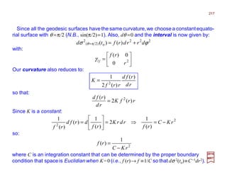


![)sin()()( 2222222
o
2
ϕθθ drdrrdtRtsd ++=
2017
MRT
If we consider ds2(t) with k =0 but at a time to, the interval becomes, with dt=0 (at t =to,
a constant):
We now pose the change of variable χ =R(to)r, a new coordinate. It is obviously the
interval of Euclidean space-time (k=0):
)sin()( 22222
o
2
ϕθθχχ dddtsd ++=
Now for k =+1, we define again a new coordinate:
2
2
2
1 r
rd
d
−
=χ
Integrating:
r
r
dr
d 1
2
sin
1
−
=⇒
−
= ∫∫ χχ
or:
χsin=r
So, at t=to:
)]sin(sin[)()( 22222
o
2
o
2
ϕθθχχ dddtRtsd ++=
This is the interval of a three-sphere of radius R(to). This model is said to be the
closed or spherically symmetric Robertson-Walker metric.
220](https://image.slidesharecdn.com/2-170115192041/85/PART-II-2-Modern-Physics-220-320.jpg)
![χsinh=r
2017
MRT
Finally, for k =−1, a similar coordinate transformation as for k =+1 gives us:
and, at t=to:
)]sin(sinh[)()( 22222
o
2
o
2
ϕθθχχ dddtRtsd ++=
This model is said to be the open or hyperbolic Robertson-Walker metric.
22222
)( σdtRtdcsd +−=
In summary, we can write:
where dσ is the interval of the Riemannian three-space of constant curvature which is
independent of time. Its interval can be written as:
)sin()( 222222
ϕθθχχσ ddfdd ++=
where f(χ) depends of the sign of the curvature. We renormalized the scale factor so
that we have three values possible – k =−1, 0, or +1. The function:
−=
=
+=
=
)1(sinh
)0(
)1(sin
)(
k
k
k
f
for
for
for
χ
χ
χ
χ
determines how the surface of the sphere χ = constant change with the radius χ. The
coordinate χ varies from 0 to ∞ if k =0 or −1. If k =+1, it varies from 0 to π. When k =−1,
the space is said to have hyperbolic geometry (Lobatschewaski), and when k =0, we
have a Euclidian geometry (i.e., flat space). For k =+1, the geometry is spherical.
221](https://image.slidesharecdn.com/2-170115192041/85/PART-II-2-Modern-Physics-221-320.jpg)


![jijitiittt tRgggcg γ)(0 22
===−= and,
2017
MRT
The exact solutions of dσ 2 =dχ2 +f 2(χ)(dθ 2 +sin2θ dϕ 2) describe spaces of symmetry.
The Friedman-Lemaître spaces are such spaces the possess high symmetry. They have
exact symmetry about each point. This implies that space-time is spatially homogeneous
and admits a group of six isomeries such that orbits are three-spaces with space-like
curvature. Minkowski space and de Sitter space are examples of Friedman-Lemaître
spaces with even more symmetries associated with them. Thus, from ds2 (t)=−c2dt2 +
R2(t)[dr2/(1−kr2)+r2dθ 2+r2sin2θ dϕ 2] the componentsof the Robertson-Walkermetric are:
Here, t is the cosmic time (a.k.a., time since the big bang); i and j are three comoving
coordinates r, θ, and ϕ. γij is the metric for a maximally symmetric space-time in three
dimensions:
( )jirr
rk
ijjirr ≠====
−
= forand,, 0sin
1
1 222
2
γγθγγγ ϕϕθθ
or, in matrix form:
−
−
=
θ
νµ
222
22
2
2
2
sin)(000
0)(00
00
1
)(
0
000
rtR
rtR
rk
tR
c
g
225](https://image.slidesharecdn.com/2-170115192041/85/PART-II-2-Modern-Physics-225-320.jpg)

![)(
)(
]sin)(ln[
2
1
ln
2
1
1
])(ln[
2
1
ln
2
1
)(
)(
])(ln[
2
1
ln
2
1
11
)(
ln
2
1
ln
2
1
)(
)(
1
)(
ln
2
1
ln
2
1
222
22
22
22
2
2
2
tR
tR
rtR
t
g
t
r
rtR
r
g
r
tR
tR
rtR
t
g
t
rk
rk
rk
tR
r
g
r
tR
tR
rk
tR
t
g
t
tt
rr
tt
rr
r
rr
rr
r
rt
r
tr
&
&
&
=
∂
∂
=
∂
∂
=Γ=Γ
=
∂
∂
=
∂
∂
=Γ=Γ
=
∂
∂
=
∂
∂
=Γ=Γ
−
=
−∂
∂
=
∂
∂
=Γ
=
−∂
∂
=
∂
∂
=Γ=Γ
θϕϕ
ϕ
ϕ
ϕ
ϕ
θθ
θ
θ
θ
θ
θθ
θ
θ
θ
θ
2017
MRT
From Type A):
and:
r
rtR
r
g
r
rr
1
]sin)(ln[
2
1
ln
2
1 222
=
∂
∂
=
∂
∂
=Γ=Γ θϕϕ
ϕ
ϕ
ϕ
ϕ
227](https://image.slidesharecdn.com/2-170115192041/85/PART-II-2-Modern-Physics-227-320.jpg)
![θθ
θ
ϕϕ
ϕϕ
θθ
θθ
ϕϕ
ϕϕ
θθ
θθ
22222
22
222
22
2
2
222
2
2
2
22
2
222
2
2
sin)1(]sin)([
]1)([2
1
2
1
)1(])([
]1)([2
1
2
1
)1(
]sin)([
)(2
1
2
1
)()(
])([
)(2
1
2
1
1
)()(1
1
)(
)(2
1
2
1
rkrrtR
rrktRr
g
g
rkrrtR
rrktRr
g
g
c
rkr
rtR
tct
g
g
c
tRrtR
rtR
tct
g
g
rk
tRtR
crk
tR
tcr
g
g
rr
r
rr
r
tt
t
tt
t
rr
tt
t
rr
−−=
∂
∂
−
−=
∂
∂
−=Γ
−−=
∂
∂
−
−=
∂
∂
−=Γ
−
−=
∂
∂
−
−=
∂
∂
−=Γ
=
∂
∂
−
−=
∂
∂
−=Γ
−
=
−∂
∂
−
−=
∂
∂
−=Γ
&
&
2017
MRT
From Type B):
and:
θθθ
θ
ϕϕ
θθ
θ
ϕϕ cossin]sin)([
])([2
1
2
1 222
22
−=
∂
∂
−=
∂
∂
−=Γ rtR
rtRr
g
g
From Type C): All other connections are zero.
228](https://image.slidesharecdn.com/2-170115192041/85/PART-II-2-Modern-Physics-228-320.jpg)


![2017
MRT
...
and:
2
)(
)(
)(
)(
)(
)(
−=
∂
∂
=
∂
Γ∂
tR
tR
tR
tR
tR
tR
tt
t
&&&&ϕ
ϕ
)()()()]()([
cossin)cossin(
sinsin3]sin)1([
sin
1
)(cot
1
sin)(
lnln
cot
1
sin)(
lnln
13)]1([
2222
22
22222
22
23
2
2
2
2
2
23
22
tRrtRrtRtRrtR
tt
rkrkr
rr
rk
rtR
g
rk
rtR
g
rkrkr
rr
t
r
r
&&&& +=
∂
∂
=
∂
Γ∂
−=−
∂
∂
=
∂
Γ∂
−=−−
∂
∂
=
∂
Γ∂
−=
∂
∂
=
−∂
∂
=−
∂
∂
=
−∂
∂
=−
∂
∂
−=−−
∂
∂
=
∂
Γ∂
θθ
θ
ϕϕ
ϕϕ
θθ
θθθθ
θθ
θθθ
θ
θ
θ
θ
θθ
θ
θ
θθ
232](https://image.slidesharecdn.com/2-170115192041/85/PART-II-2-Modern-Physics-232-320.jpg)

![2017
MRT
… so:
222
22
2
2
2222
22
222
22
2
2
222
22
2
2
2
1
2
)1(1
)(
3
2
1)1(
2
2
)1(1
)(
2
1)1(
2
1
)(
1
)()(
rk
k
rk
rk
rk
tR
rrk
k
rk
rk
rrk
rk
rk
tR
rk
k
rk
rk
rk
tR
rk
tRtR
R rr
−
−
−
−
−
−−
−
+
−
+
++
−
+
−
+
−
−
−
−
−
−
−
−=
&
&&&&
and:
22
2
2
1
2
1
)(2
1
)()(
rk
k
rk
tR
rk
tRtR
R rr
−
−
−
−
−
−=
&&&
and now, finally:
2
2
1
1
]2)(2)()([
rk
ktRtRtRR rr
−
−−−= &&&
Since space is isotropic, Rθθ and Rϕϕ have the same form as this previous equation:
22
]2)(2)()([ rktRtRtRR −−−= &&&
θθ
θϕϕ
222
sin]2)(2)()([ rktRtRtRR −−−= &&&
and:
234](https://image.slidesharecdn.com/2-170115192041/85/PART-II-2-Modern-Physics-234-320.jpg)
![jijiittt kRRRRR
R
R
R γ)22(03 2
++−=== &&&
&&
and,
2017
MRT
The Ricci tensor then has the components:
We also need to calculate the scalar curvature:
2
2
22
2
2
2
22
2
666
6633
3
)22(3
))(22(3))(22(3
])22([
R
k
R
R
R
R
R
k
R
R
R
R
R
R
R
kRRR
R
R
gggkRRR
R
R
gkRRR
R
R
kRRRgRRgRgRgR
rr
rr
i
ii
ii
i
ii
ii
tt
i
ii
ii
tt
tt
−
−−=
−+−−=
++−−=
++++−−=++−−=
++−+−=+==
∑
∑∑∑∑
&&&
&&&&&
&&&
&&
&&&
&&
&&&
&&
&&&
ϕϕ
ϕϕ
θθ
θθ
µ ν
µν
µνµ
µ
γγγγ
γ
so that (for µ =t,r,θ, or ϕ):
+
+−= 2
2
6
R
k
R
R
R
R
R
&&&µ
µ
235](https://image.slidesharecdn.com/2-170115192041/85/PART-II-2-Modern-Physics-235-320.jpg)


([
3
π4
3
tpt
G
R
R
+−
Λ
= ρ
&&
241](https://image.slidesharecdn.com/2-170115192041/85/PART-II-2-Modern-Physics-241-320.jpg)


![)(
3
π8
32
2
t
G
R
k
R
R
ρ+
Λ
+−=
&
2017
MRT
We now look to find R(t) and for that we go back to the initial value equation obtained
earlier:
and since:
)1(π43π4
)(
)(
)()( o
2
oo2
o
2
ooo3
3
o
o3
o
3
o +−=−=Λ== qHG
R
k
HqG
R
R
tR
tR
tt ρρρρρ and,
we get:
3
3
o
o2
2
o
2
o
2
3
π8
3 R
RG
R
R
R
k
R
R
ρ+
Λ
+−=
&
then:
3
3
o
o
2
ooo2
2
o
o
2
oo
2
3
π8
)3π4(
3
1
)]1(π4[
R
RG
HqG
R
R
qHG
R
R
ρρρ +−++−−=
&
R
RG
RHqR
G
RqHRGtR
3
o
o
22
oo
2
o
2
oo
2
o
2
oo
2
3
π8
3
π4
)1(π4)( ρρρ +−+++−=&
and finally:
247](https://image.slidesharecdn.com/2-170115192041/85/PART-II-2-Modern-Physics-247-320.jpg)


![)(
3
π8
32
2
t
G
R
k
R
R
ρ+
Λ
+−=
&
2017
MRT
We can express this integral as a function of only Ωo and Λ by using our equation for
R/R again:
222
)(
3
π8
3
Rt
G
RkR ρ+
Λ
+−=&
to give us:
22
ooo
2
o
2
o
o
2
32
3
1
3
π8
RRqH
R
RG
R
Λ
+
Ω−++= ρ&
With ρ(t)=ρ(to)[R3(to)/R3(t)] and k/Ro
2=−Ho
2[qo+1−(3/2)Ωo]:
∫∫
Λ
+Ω−+
Ω=
−
)(
)(
2/1
2
o
2
o
2
o
o
o
2
oo
oo
)(
3
)1(
)(
)(
tR
tR
t
t
tRRH
tR
R
RHtRdtd
Furthermore, with ρo =3Ho
2qo/4πG and Ωo =2qo, all of this gives us:
⋅⋅⋅⋅
)(
3
)1(
)(
)( 2
o
2
o
2
o
o
o
2
o
2
o
2
tRRH
tR
R
RH
td
tRd Λ
+Ω−+
Ω=
so that:
250](https://image.slidesharecdn.com/2-170115192041/85/PART-II-2-Modern-Physics-250-320.jpg)

![(ρo = 0) 0.0
0.5
Ωo
ΩΛ
10.0
5.0
0.0
0.40
0.63
0.86
1.10
1.33
1.57
∫
Ω+Ω−+Ω=×
−
Λ
−
1
0
2/1
3
2
o
oo
2/11
oo
3
π8
)1()( χχχχ
H
G
dHt
(1)
(3)
(5)
(4)
(7)
(8)
(ρo = ρc) 1.0
(2)
(Λ=0)
(9)
(6)
252
Exercise: Calculate the age of
the universe (in yr) integral for a
more current value of the Hubble
constant of Ho =67.7 km/s/Mpc
[Planck Mission (2013)], density
parameter of Ωo =1.02, and
vacuum density of ΩΛ =0.692
[WMAP (2003)].
Here is the result of plotting this definite integral for the cosmic time to as a function of
thedensity parameter Ωo =ρo/ρc (ρc being the critical density)and thevacuum density ΩΛ.
This composite plot shows the age of the universe, to (×Ho
−1), for 1) variable Ωo for ΩΛ =−ρc; 2) variable
Ωo for ΩΛ =0 (i.e., the cosmological constant Λ=0); 3) variable Ωo for ΩΛ =ρc; 4) variable Ωo for ΩΛ =
5ρc; 5) variable Ωo for ΩΛ =10ρc; 6) variable ΩΛ for Ωo =0 (i.e., when ρo =0); 7) variable ΩΛ for Ωo =0.1;
8) variable ΩΛ for Ωo =0.5; and 9) variable ΩΛ for Ωo =1.0 (i.e., when ρo = ρc).
)(
)(
3π8
8π
3
o
o
oo
o
tR
tR
H
HG
G
H
c
c
c
&
=
Λ
=
Λ
=Ω
==Ω
Λ and
,with
ρ
ρ
ρ
ρ
( )
)(givenyearsbillion12oryr
km/s/Mpcif
yr
o
9
o
0
1
19o
1012
55
)1018(
1
3
2
o
H
Ht
×=
=
×
=
=Λ
=Ω
−
2017
MRT](https://image.slidesharecdn.com/2-170115192041/85/PART-II-2-Modern-Physics-252-320.jpg)


PART II.2 - Modern Physics
- 1. From First Principles PART II – MODERN PHYSICS May 2017 – R2.1 Maurice R. TREMBLAY http://atlas.ch Candidate Higgs Decay to four muons recorded by ATLAS in 2012. Chapter 2
- 2. Contents PART II – MODERN PHYSICS Charge and Current Densities Electromagnetic Induction Electromagnetic Potentials Gauge Invariance Maxwell’s Equations Foundations of Special Relativity Tensors of Rank One 4D Formulation of Electromagnetism Plane Wave Solutions of the Wave Equation Special Relativity and Electromagnetism The Special Lorentz Transformations Relativistic Kinematics Tensors in General The Metric Tensor The Problem of Radiation in Enclosures Thermodynamic Considerations 2017 MRT The Wien Displacement Law The Rayleigh-Jeans Law Planck’s Resolution of the Problem Photons and Electrons Scattering Problems The Rutherford Cross-Section Bohr’s Model Fundamental Properties of Waves The Hypothesis of de Broglie and Einstein Appendix: The General Theory of Relativity References 2
- 3. 3 2017 MRT 1. Space is isotropic and homogeneous; that is, the equations of motion of mechanics are unchanged by rotations and translations (or leaps) of the coordinate systems used to describe the positions of particles, when the rotations and translations do not depend on time as a parameter; 2. Time is independent of space; essentially, that is a parameter that measures the separation between events as seen by an observer, and the observer’s location does not affect the size of the standard intervals used to measure time; 3. Time is homogeneous; the equations of motion of mechanics are unchanged by a displacements (or translations) in the time parameter t; 4. The equations of motion of mechanics are unchanged by spatial translations that involve time as a linear parameter; that is, translations expressible in the form r→r−vt. Frames of reference (i.e., a set of coordinate axes) related by such transformations are called inertial frames, and the transformations are called Galilean transformations; 5. Time is independent of inertial reference frame (i.e., an observer’s state of inertial motion does not affect the scale of time measurements). Thus one has a picture of the world as a homogeneous and isotropic three-dimensio- nal structure of space-points, with particles passing through these points according to laws formulated in terms of a parameter t called time; an important property of the classi- cal laws governing particle motion is that these laws are the same for all frames of refe- rence moving with uniform velocity v relative to one another (i.e., classical mechanical laws are the same for all frames related to one another by Galilean transformations). Foundations of Special Relativity Maxwell published his set of equations between 1861 and 1862. After that, and up until 1905, the following five statements enumerate some of the properties of space and time as they were know by physicists at the time:
- 4. For the description of processes taking place in nature,* one must have a system of reference. By a system of reference we understand a system of coordinates serving to indicate the position of a particle in space, as well as clocks fixed in this system serving to indicate the time. 4 2017 MRT There exists a system of reference in which a freely moving body (i.e., a moving body which is not acted upon by external forces) proceeds with constant velocity. Such reference systems are said to be inertial. * These next 3 slides are taken from L. Landau & E. Lifshitz, The Classical Theory of Fields, 4-th Ed., B-H (1975), pp. 1-2. If two reference systems move uniformly relative to each other, and if one of them is an inertial system, then clearly the other is also inertial (N.B., in this system too every free motion will be linear and uniform). In this way one can obtain arbitrarily many inertial systems of reference, moving uniformly relative to one another. Experiment shows that the so-called principle of relativity is valid. According to this principle all the laws of nature are identical in all inertial systems of reference. In other words, the equations expressing the laws of nature are invariant with respect to transformations of coordinates and time from one inertial system to another. This means that the equation describing any law of nature, when written in terms of coordinates and time in different inertial reference systems, has one and the same form. The interaction of material particles is described in ordinary mechanics by means of a potential energy of interaction, which appears as a function of the coordinates of the interacting particles. It is easy to see that this manner of describing interactions contains the assumption of instantaneous propagation of interactions.
- 5. For the forces exerted on each of the particles by the other particles at a particular instant of time depend, according to this description, only on the positions of the particles at this one instant. A change in the position of any of the interacting particles influences the other particles immediately. 5 2017 MRT However, experiment shows that instantaneous interactions do not exist in nature. Thus a mechanics based on the assumption of instantaneous propagation of interac- tions contains within itself a certain inaccuracy. In actuality, if any change takes place in one of the interacting bodies, it will influence the other bodies only after the lapse of a certain interval of time. It is only after this time interval that processes caused by the initial change begin to take place in the second body. Dividing the distance between the two bodies by this time interval, we obtain the velocity of propagation of the interaction. We note that this velocity should, strictly speaking, be called the maximum velocity of propagation of interaction. It determines only that interval of time after which a change occurring in one body begins to manifest itself in another. If is clear that the existence of a maximum velocity of propagation of interactions implies, at the same time, that motions of bodies with greater velocities than this are in general impossible in nature. For if such a motion could occur, then by means of it one could realize an interaction with a velocity exceeding the maximum possible velocity of propagation of interactions. Interactions propagating from one particle to another are frequently called ‘signals’, sent our from the first particle and ‘informing’ the second particle of charges which the first has experienced. The velocity of propagation of interaction is then referred to as the signal velocity.
- 6. From the principle of relativity it follows in particular that the velocity of propagation of interactions in the same in all inertial system of reference. Thus the velocity of propagation is a universal constant. This constant velocity is also the velocity of light in empty space. The velocity of light is usually designated by the letter c, and its numerical value is: 6 2017 MRT The large value of this velocity explains the fact that in practice classical mechanics appears to be sufficiently accurate in most cases. The velocities with which we have occasion to deal are usually so small compared with the velocity of light that the assumption that the latter is infinity does not materially affect the accuracy of the results. m/s8 10998.2 ×=c The combination of the principle of relativity with the finiteness of the velocity of propagation of interactions is called the principle of relativity of Einstein (formulated in 1905) in contrast to the principle of relativity of Galileo, which was based on an infinite velocity of propagation of interactions. The mechanics based on the Einsteinian principle of relativity is called relativistic. In the limiting case when the velocities of the moving bodies are small compared to the velocity of light we can neglect the effect of the motion of the finiteness of the velocity of propagation of interactions; this mechanics is called Newtonian or classical. The limiting transition from relativistic to classical mechanics can be produced formally by the transition to the limit c→∞ in the formulas of relativistic mechanics.
- 7. The principle of Galilean invariance then asserts that the ‘laws of nature’ are the same for two observers, i.e., that the form of the equations of motion is the same for both observers. The equations of motion must therefore be covariant with respect to the transformations r=r +vt and t =t. Unfortunately, this invariance principle applies only in situations where the velocity v is much lower than that of light. We need more… Experiments have also yielded the fact that space is isotropic so that the orientation in space of an event is an irrelevant initial condition and this principle can be translated into the statement that: ‘the laws of motion are invariant under spatial rotations.’ Newton’s law of motion further indicated that the state of motion, as long as it is uniform with constant velocity, is likewise and irrelevant initial condition. This is the principle of Galilean invariance which assets that the laws of nature are independent of the velocity of the observer, and more precisely, that the laws of motion of classical mechanics are invariant with respect to Galilean transformations: τ+→+→ ttandarr − = ⇔ = −= tttt t rvrvrr 10 1 The laws of nature are independent of the position of the observer or, equivalently, that the laws of motion are covariant with respect to displacements in space and time, i.e., with respect to the transformations: 2017 MRT 7 We now look at the role played by invariance principles (i.e., changes in points of view must not change the laws used to describe them) in the formulation of physical theories.
- 8. The acceleration of a particle is the time derivative of its velocity (i.e., ax =dux /dt, &c). To find the Galilean acceleration transformations we differentiate the velocity transfor- mations above (using the fact that t=t and v is considered a constant) to obtain: The relationship between [ux,uy,uz] and [ux,uy,uz] is obtained from the time differen- tiation of the Galilean coordinate transformation x ↔x. Thus, from r=x i and x =x −vt: vuv td xd td td td vtxd td vtxd td xd u xx −= −= − = − == )1( )()( 2017 MRT where −v is the velocity of frame S relative to S. Altogether, the Galilean velocity transfor- mations are: zzyyxx uuuuvuu ==−= and, zzyyxx aaaaaa === and, Thus the measured acceleration components are the same for all observers moving with uniform relative velocity. (N.B., That is why v was chosen to be a constant since it gives us a uniform relativistic motion to deal with otherwise things get really complicated). 8 ˆ In addition to the coordinate of an event, the velocity of a particle is of interest. Two ob- servers, O and O, will describe the particle’s velocity by assigning three components to it, with [ux,uy,uz] being the velocity components as measured by O in frame S and [ux,uy,uz] being the velocity components as measured by O (i.e., relative to frame S).
- 9. Since, in elementary mechanics, longitudinal sound waves and transverse waves along a string are familiar phenomena, one might expect that electromagnetic waves should obey the same laws that govern such mechanical waves. Such a situation would be very desirable, for then the physics of electromagnetism might be unified conceptually with the physics of massive bodies. Let us therefore test the applicability of classical mechanics to electromagnetic theory by carrying out a Galilean transformation on the wave equation governing electromagnetic waves. 9 2017 MRT We are interested in the telegrapher’s equation: 0),( 1 2 2 2 2 = ∂ ∂ −∇ tf tc r where f (r,t) is a scalar function of r ≡ri and t. Now, under a Galilean transformations,ri →ri =ri −vit, and since f (r,t) is a scalar function, it must have the same numerical value in both coordinate systems, although its form as a function of r and t may be different. Thus, let: ]),,([),(),( ttgtgtf rrrr == where the last member demonstrates that g depends of t implicitly through the dependence of r(r,t) on t, as well as explicitly.
- 10. Now we have: 10 2017 MRT jj j jj k k jk k kj k j r tg r tg r tg r tg r r r tf ∂ ∂ = ∂ ∂ = ∂ ∂ = ∂ ∂ ∂ ∂ = ∂ ∂ ∑∑∑= ),(),(),(),(),( 3 1 rrrrr δδ since δk j =∂rk /∂rj has the definition δkj =1 when k= j and δkj =0 when k≠ j, so that: ),(),( 22 tgtf rr ∇=∇ However: t tg tg t tg r tg t r t tf k k k ∂ ∂ +•= ∂ ∂ + ∂ ∂ ∂ ∂ = ∂ ∂ ∑= ),( ),( ),(),(),( 3 1 r rv rrr ∇∇∇∇ and: 444444 3444444 21 incouplingordersecondandFirst ∇∇∇∇ ∇∇∇∇∇∇∇∇∇∇∇∇ • ••+ ∂ ∂ •+ ∂ ∂ = ∂ ∂ v rvv r v rr )],([ ),( 2 ),(),( 2 2 2 2 tg t tg t tg t tf Therefore, the telegrapher’s equation transforms Galileanly according to the rule: 0),( 1 2),( 1 2 2 22 2 2 2 2 2 = ∂ ∂ − ∂ ∂ •− • •−∇= ∂ ∂ −∇ tg tctccc tf tc r vvv r ∇∇∇∇∇∇∇∇∇∇∇∇ or 0),()()(2 1 ),( 1 2 2 2 2 2 2 2 2 2 = •+ ∂ ∂ •+ ∂ ∂ −∇= ∂ ∂ −∇ tg ttc tf tc rvvr ∇∇∇∇∇∇∇∇ Yikes!
- 11. Evidently, the equation governing electromagnetic wave propagation has a different form in the bared reference frame, with coordinate ri, from that which it has in the ‘un- bared’ reference frame, with coordinate ri. The form of the telegrapher’s equation is not invariant under Galilean transformations. Since this equation represents the law of electromagnetic wave propagation, one might say that the choice of Galilean reference frame affects the laws of electromagnetism. Based on this argument alone, Galilean invariance cannot be considered further. 11 2017 MRT Classical mechanics and electromagnetism therefore cannot be welded together without some changes. But which theory should we retain, if either? As it turned out, both theories can be retained almost intact, but Newtonian mechanics has had to yield a little bit by giving up, as an exact postulate, the invariance of the equations of motion under Galilean transformations, together with the notion that time is independent of reference frame. The only way this question could be answered, however, was to turn to experiment and to try to determine physically whether the constant c that appears in the telegrapher’s equation refers to the velocity of wave propagation in some preferred reference frame (i.e., the frame of reference in which the “ether” or ‘propagating medium’ is a rest, presumably) so that Maxwell’s equations are strictly correct only in that preferred frame, or whether some aspect of mechanics is a defective description of nature. Since Maxwell’s equations were relative newcomers to physics, it is not surprising that the main experimental effort was aimed at detecting a preferred frame of reference to which electricity and magnetism always should be referred.
- 12. According to Coulomb’s law, fC(r)= (1/4πεo)ρ(r)∫∫∫V ρ(r)[(r−−−−r)/|r−−−−r|3]d3r, and the law of Biot and Savart, fBS(r)= (µo/4π)J(r)××××∫∫∫V J(r)××××[(r−−−−r)/|r−−−−r|3]d3r, the total force f(r) per unit volume exerted on a charge density ρ(r) and current density J(r) is: 12 2017 MRT )()()()()()()( BSC rBrJrErrfrfrf ××××++++++++ ρ== Now if the charge density vanishes everywhere except at a single point ro, and is so large at ro that ∫∫∫V ρ(r)d3r=q is a finite number (if ro is in V of course), then we can write: ˆ )()( orrr −−−−δρ q= that is, we have a point charge of magnitude q at ro. Similarly, if J(r) is generated by a point charge of magnitude q moving with velocity v(r), have: )()()()()( oo rrrvrvrrJ −−−−δρ q== when the charge is at ro. )]()([)()]()([ )]()()()([)( ooo 33 rBrrrvrErr rrBrJrErrrfF ××××−−−−++++−−−− ××××++++ δδ ρ qq dd VV = == ∫∫∫∫∫∫ so that we obtain: )]()()([ ooo rBrvrEF ××××++++q= With these expressions for the charge and current densities,the total force experienced by the charge evidently is: This is the Lorentz force law, which is in this case, as seen from an origin O, ro away.
- 13. The field vectors E(r) and B(r) can be written in terms of the scalar and vector potentials, according to E(r)= −∇∇∇∇φ(r)−−−−∂A(r)/∂t and B(r)= ∇∇∇∇××××A(r), and for fields gene- rated by a point charge q at r, the potentials given by φ(r)=(1/4πεo)∫∫∫V ρ(r)(1/|r−−−−r|)d3r and A(r)=(µo/4π)∫∫∫V J(r)(1/|r−−−−r|)d3r] become: 13 2017 MRT rr rv rA rr r −−−−−−−− )( π4 µ )( 1 επ4 )( o o qq == andφ where v(r) is the velocity of the source charge q. If the velocity v(r) is a constant, we then have: )( π4 µ )( )( επ4 )( 3 o 3 o rv rr rr rA0 rA rr rr r ×××× −−−− −−−− ××××∇∇∇∇ −−−− −−−− ∇∇∇∇ q t q −== ∂ ∂ =− and,φ Therefore the fields at point r arising from a uniformly moving charge q at r are: 3 o 3 o )()( π4 µ )( επ4 )( rr rrrv rB rr rr rE −−−− −−−−×××× −−−− −−−− qq == and The force on charge q at ro due to these fields is: )]}()([)(εµ){( 1 επ4 )]()()([ ooooo3 oo ooo rrrvrvrr rr rBrvrEF −−−−××××××××++++−−−− −−−− ××××++++ qq q == where the first term is the electromagnetic force and the second is the magnetic force. This is familiar from elementary physics of point charges.
- 14. Now the torque ττττ on the charge at ro about the point r is defined to be: 14 )]([ π4 µ 3 o rvvr ××××××××××××ττττ r qq = Note that the torque arises entirely from magnetic effects! )]}()([)({)( π4 µ )( ooo3 o o o rrrvrvrr rr Frr −−−−××××××××××××−−−− −−−− ××××−−−−ττττ qq == Consider the arrangement shown in the Figure, for which we take v(r)=v(ro)=v. Here we have: Schematic diagram of the arrangement of the Trauton-Noble experiment. If the angle between v and r is θ, the multiple cross-pro- duct on the right-hand side can be rewritten in terms of θ as: where r××××v ≡(r××××v)/|r××××v| is a unit vector in the direction of r××××v. Hence the torque tending to restore the vector r to an orientation perpendicular to v is (N.B., we use c2 =1/µoεo): 2017 MRT where r=ro −−−−r. vr vr vrrvrvrvrrvvr ×××× ×××× ××××−−−−×××××××××××××××× ˆ2sin 2 1 ˆcossin ))((])[()]([ 22 22 2 θ θθ rv rv v = = •=•= ˆ vr ××××ττττ ˆ2sin επ4 1 2 o θ = c v r qq v r v q Pivot q _ ro r O v××××(v×××× r) r××××vˆ θ 2 π θ − 2 π ττττ
- 15. At this point, we must ask: With respect to what frame of reference are we to measure v? If there were a fixed preferred frame of reference to which all electromagnetic effects should be referred, then v certainly would be measured relative to that frame. 15 2017 MRT In 1903, Trauton and Noble performed a series of experiments in which charged condensers were moved through space at the velocity of the earth relative to the sun; the apparatus was sufficiently sensitive to detect torques resulting from velocities somewhat less than earth’s orbital velocity, the former presumably being measured relative to some preferred reference frame. However, no torque relative to the preferred frame, or the “ether”, than is the sun; thus, if one accepts the notion of an absolute frame of reference for electromagnetic effects, one apparently is forced by this experiment to reconsider the possibility of a Ptolemaic or geocentric theory of the universe. A more reasonable alternative is to question the notion of a preferred reference frame, and to reason that in the absence of such a preferred frame we cannot make sense of ττττ=(1/4πεo)(qq/r)(v/c)2sin(2θ )r××××v until the meaning of the velocity v is clarified (i.e., until the manner in which v is to be measured relative to an arbitrary frame is specified). ˆ At about the same time, Michelson and Morley, and many others, carried out an experiment using an interferometer; this interferometer produced circular fringes and from these fringe patterns, they meant to measure an effect predicted by the notion of an “ether” that sustains electromagnetic waves and that is stationary relative to the preferred reference frame… None of them observed any significant phase shift! _
- 16. It is a fundamental postulate of Physics that the laws of nature be expressed by equations that are valid for all coordinate systems (i.e., locally inertial reference frames). Alternatively, we say that the laws of nature are covariant, which means that they have the same forms in all coordinate systems. A systematic method of investi- gating the behavior of quantities that undergo a coordinate transformation is the subject matter of tensor analysis. In developing the mathematical subject of absolute differential geometry, Gauss, Riemann, and Christoffel (1829-1900) introduced the concept of a tensor. The subject of absolute tensor calculus (i.e., tensor analysis) was introduced and developed by Ricci (1853-1925) and his student Levi-Civita (1872-1941). Einstein (1879- 1955) made extensive use of tensors (i.e., technically called differential tensor calculus) in his formulation of the general theory of relativity. Insofar, a tensor consists of a set of quantities, called components, whose properties are independent of the coordinate system used to describe them. The components of a tensor in two different coordinate systems are related by the characteristic tensor transformation as discussed below. 2017 MRT Now a word on notation. A collection of indices (subscripts and/or superscripts) is used to make the mathematical development of tensor analysis compact. The superscripts, contravariant indices, are used to denote the contravariant components of a tensor, Tij.... The subscripts, covariant indices, are used to represent the covariant compon- ents of a tensor, Tij.... The components of a mixed tensor are specified by indicating both subscripts and superscripts (or a jumble of superscripts and subscripts), Ti k j m k n ... .... For ever more will we will use this notation (Latin letters or Greek symbols; lower or upper case; bold, italized or not, to denote the components of a tensor or the tensor itself.) 16 Tensors of Rank One
- 17. defines a new coordinate system specified by the mutually independent variables: x1, x2, …, xn. The symbol φ i (e.g., a temperature distribution or field of some sort) are ass- umed to be single-valuedreal functions of the coordinates with continuous derivatives. The rank (order) of a tensor is the number (without counting an index which appears once as a subscript and once as a superscript) of indices in the letter or symbol representing a tensor (or the components of a tensor). Here a few examples of tensor (and their rank) which will make an appearance very soon: S is a tensor of rank zero (scalar – e.g., action); xi is a covariant vector of rank one (covariant vector – e.g., three- dimensional Cartesian coordinate); Pµ is a contravariant tensor of rank one (contra- variant vector – e.g., space-time momentum); Tµ ν is a mixed tensor of rank two (e.g., energy-momentum-stress tensor) ; Gµν =Rµν +½gµνR is a (contravariant–e.g., Einstein’s gravitational field tensor) tensor of rank two; Rµν ≡Σλ Rλ µλν (note the contraction on the index λ) is a tensor (e.g., Ricci curvature tensor) of rank two; Rµ νρσ is a mixed tensor (e.g., action Riemann curvature tensor) of rank four; and finally R ≡ΣµΣν gµν Rµν (i.e., another contrac-tion on both µ andν) is a tensor of rank zero (scalar – e.g., curvature scalar). In an n-dimensional space, the number of components of a tensor of rank n is nr. ( )nixxxx nii ,,2,1),.,,( 21 KK == φ Consider a ordered set of n mutually independent real variables x1,x2,…,xn =[xi], called the coordinate of a point, Pn(x1,x2,…,xn). The collection of all such points corresponding to all the sets of values [xi] forms an n-dimensional linear space (i.e., a manifold – French for variété) which we specify by Vn. The set of n equations: 2017 MRT 17
- 18. On differentiating xi =φ i(x1, x2, …, xn) (N.B., xi for x is the same as xi for an index i) with respect to x j, we obtain the following representation for an infinitesimal displacement in the original coordinate system, xj, in terms of the new coordinate system, x i: ∑∑ == ∂ ∂ = ∂ ∂ = ∂ ∂ ++ ∂ ∂ + ∂ ∂ = n j j j in j j j i n n iii i xd x x xd x xd x xd x xd x xd 11 2 2 1 1 φφφφ K A set of components, Aj, which transform according to the law above, which is given by the same process: 2017 MRT If det|∂xi/∂x j|≠0 (i.e., the Jacobian is non-zero) then the inverse transformation exists. ∑= ∂ ∂ = ∂ ∂ ++ ∂ ∂ + ∂ ∂ = n j j j i n n iii i A x x A x x A x x A x x A 1 2 2 1 1 K forms the transformation law for the components of a contravariant tensor of rank one. As a quick example of its use, let us find the transformation for rotation in two dimensions. In this case, we have: x1 =x1cosθ + x2sinθ and x2 =x2cosθ − x1sinθ. The Jacobian of the transformation is given by: 1sincos)sin()(sincoscos cossin sincos det 22 2 2 1 2 2 1 1 1 =+=−⋅−⋅= − == ∂ ∂ ∂ ∂ ∂ ∂ ∂ ∂ ∂ ∂ θθθθθθ θθ θθ x x x x x x x x j i x x 18
- 19. In this last equation (i.e., Ai =Σj (∂xi/∂xj)Aj) Aj is a function of the coordinates x j (i.e., Aj = Aj(x j)) and Ai is a function of the coordinates xi (i.e., Ai =Ai(xi)), where x j and xi refer to the old and new coordinate systems, respectively. 2017 MRT where the Kronecker delta,δ k j, is given by: or changing the dummy index k to j: ∑= ∂ ∂ = n i i i j j A x x A 1 ≠ = = kj kj k kk j 0 1 when )for,(when δ δ e.g. k k n k k n j jk j n n kn i n j j j i i kn i n j j j i i kn i i i k A AA AA x x A x x A x x x x A x x = ⋅=⋅= = ∂ ∂ = ∂ ∂ = ∂ ∂ ∂ ∂ = ∂ ∂ ∑ ∑∑ ∑∑∑∑ ∑∑ = = == == == == 1 1 11 11 11 11 )( k k k j i j j j i i x x δ δδ ∂∂∂∂ ∂∂∂∂ The equation Ai =Σj (∂xi/∂xj)Aj may be solved for Aj if it is multiplied by ∂xk/∂xi and summed over i. In this case, we obtain: 19
- 20. A set of quantities Bk is called the components of a covariant tensor of rank one if: 2017 MRT for an arbitrary contravariant tensor with components Ak. If Ak from Ak =Σi(∂xk/∂xi)Ai is substituted into Σk Ak Bk =Σk AkBk, the result is: ∑∑∑ ∑∑∑ = == === ∂ ∂ = ∂ ∂ == n k n l l k k ln k k n i i i kn k k k n k k k BA x x BA x x BABA 1 11 111 or or ∑∑ == == n k k k n k k k BABA 11 scalar)(ainvariant 0 1 1 = ∂ ∂ −∑ ∑= = n k n l lk l k k B x x BA ∑= ∂ ∂ = n l lk l k B x x B 1 since the Ak are arbitrary. Bk =Σl(∂xl/∂xk)Bl is the transformation law for the compo- nents of a covariant tensor of rank one. An easy to remember mnemonic for the placement of ∂xi is ‘CO BELOW’ for covariant components. Now for an application… 20
- 21. Maxwell’s equations (i.e., the foundation of the theory of electromagnetism)are equa- tions that describe how electric field intensity (E) and magnetic field intensity (H) are generated and altered by each other and by charge density (ρ) and current density (J): 2017 MRT t t ∂ ∂ += =• ∂ ∂ −= =• D JH B B E D ××××∇∇∇∇ ∇∇∇∇ ××××∇∇∇∇ ∇∇∇∇ 0 ρ In MKS units, the quantity B is the magnetic induction: with εo (i.e., 8.854×10 −12 C2/N⋅m2) the permittivity of the vacuum. HB oµ= ED oε= with µo (i.e., 4π×10−7 kg⋅m/C2) being the permeability of the vacuum and quantity D is the electric displacement: form the foundation of classical electrodynamics, classical optics (N.B., with isotropic medium effects neglected), and electric circuits. Coulomb’s Law: Faraday’s Law: Absence of free magnetic poles: Ampère’s Law (∇∇∇∇•J=0): 21 These provide a set of partial differential equations that, together with the Lorentz force law: )( BvEF ××××++++q= 4D Formulation of Electromagnetism
- 22. In practice, the relation between the electric flux density D and the electric field E depends on the electric properties of the medium! Similarly, the relation between the magnetic flux density B and the magnetic field H depends on the magnetic properties of the medium. Two equations help define these relations: 2017 MRT in which P is the polarization density and M is the magnetization density. In a dielectric medium, the polarization density is the microscopic sum of the electrical dipole moments that the electric field induces. The magnetization density is similarly defined. So, in free space (i.e., P=M=0): where: EP χoε= 22 MHBPED ++++++++ oo µε == and we recover the relations obtained earlier. HBED oo µε == and A medium in the simplest case is linear, nondispersive, homogeneous, and isotropic. The vectors P and E at any position and time are parallel and proportional, so that: where χ is a scalar constantcalled the electric susceptibility.Substituting P into D=εoE+P, it follows that D and E are also parallel and proportional: ED ε= )1(εε o χ+= is another scalar constant, the electric permittivity of the medium. The ratio ε/εo is the relative permittivity or dielectric constant.
- 23. If we also consider a medium in which there are no free electric charges or currents, (i.e., ρ=0 and J=0) Maxwell’s equations in free space with εo replaced by ε simplify to: 2017 MRT 23 Each of the components of E and H therefore satisfies the wave equation: 0 ),(1 ),( 2 2 2 2 = ∂ ∂ −∇ t tf c tf r r tt ∂ ∂ ==• ∂ ∂ −==• D HH H EE ε0µ0 o ××××∇∇∇∇∇∇∇∇××××∇∇∇∇∇∇∇∇ and,, with a speed c =1/√(εµo). The different components of the electric and magnetic fields propagate in the form of waves of speed: n c c o = where: oo o o µε 1 1 ε ε =+== cn andχ The constant co is the speed of light in free space (e.g., a vacuum); the constant n is the ratio of the speed of light in free space to that in the medium called the refraction index of the medium – the refractive index is the square root of the dielectric constant! In inhomogeneous dielectric media (e.g., graded index) the coefficients χ =χ(r) and ε=ε(r) are functions of position. The refractive index n=n(r) is also position dependent.
- 24. In anisotropic media, the relation between the vector P and E depends on the direction of the vector E, and these two vectors are not necessarily parallel. If the medium is linear, nondispersive, and homogeneous, each component of P=[P1,P2, P3] is a linear combination of the three components of E=[E1,E2, E3]: 2017 MRT 24 = ++++++++= ++== ∑= 3 2 1 332313 322212 312111 o 333o223o113o332o222o112o331o221o111o 33o22o11o 3 1 o ε εεεεεεεεε εεεε E E E EEEEEEEEE EEEEP iii j jjii χχχ χχχ χχχ χχχχχχχχχ χχχχ where the indices i, j =1,2,3 denote the x, y, and z components. The dielectric properties of the medium are described by an array [χij] of 3×3 constants known as the susceptibility tensor. Also for anisotropic media, a similar relation as above between D and E applies: where [εij] are elements of the electric permittivity tensor. == ∑= 3 2 1 332313 322212 3121113 1 εεε εεε εεε ε E E E ED j jjii
- 25. Now, considering an arbitrary fluid flow situation with the Lorentz (1853-1928) condition: 2017 MRT where the d’Alembertian operator, , or d’Alembertian for short, is defined by: If this condition is satisfied, the basic equations for the vector and scalar potentials are: With definitions for the vector A (i.e., the electromagnetic vector potential) and scalar φ (i.e., the electromagnetic scalar potential) potentials, which are important parame- ters when studying Lorentz invariance concepts and non-local phenomena, we obtain: tt ∂ ∂ −=•⇔= ∂ ∂ +• φφ ΑΑ ∇∇∇∇∇∇∇∇ 0 JA oµ−= oε −= ρ φ and: 2 2 2 2 1 tc ∂ ∂ −∇= t∂ ∂ −−== A EAB φ∇∇∇∇××××∇∇∇∇ and 25
- 26. We began our discussion of special relativity by demonstrating that the demands of Maxwell’s theory of electromagnetism were not consistent with the hypotheses of Newtonian mechanics. Einstein (with Minkowski’s help) has shown us how to reformulate physics, in terms of a rather elegant four-dimensional mathematical framework, such that the two classical theories could be welded together into a unified structure. We will now work out Maxwell’s theory into the same four-dimensional framework. That this reformulation of electromagnetism will yield rather elegant and apparently simple equations should be a gratifying reward for our efforts. 26 2017 MRT vJ ρ= In our original expression for the current density vector we had: where ρ is the charge density for a distribution of charge moving with velocity v relative to an observer. This suggests that the four-vector representation for the current density might be: τ ρρ µ µµ d xd uJ == where ρ is the invariant charge density (i.e., the charge density as seen by an observer at rest relative to the charge involved). The components of the current density four- vector are given by: ],[ vργργµ cJ = which is obtained by letting dτ =(1/γ )dt with γ =1/√(1−v2/c2) and using v=dx/dt.
- 27. This discussion immediately yields an interpretation for the temporal component of J µ. Evidently, J 0 =γ ρc is just c times the charge density as seen by an observer relative to whom the charges are moving with velocity v (i.e., J 0 is c times the charge density of the charges having current density J=γ ρv). In the limit v/c<<1, we have γ ≅1, and: 27 2017 MRT vJ ρρ ≅≅ andcJ 0 as the nonrelativistic approximations for the components of the current density four- vector. A particular pleasant result of this formulation of a four-vector current density is that the equation of continuity takes a very simple form, namely: 03 3 2 2 1 1 0 0 3 0 =∂+∂+∂+∂=∂= ∂ ∂ ∑∑= JJJJJ x J µ µ µ µ µ µ and which, otherwise, would be written as: 0)( )(1 =•+ ∂ ∂ vργ ργ ∇∇∇∇ t c c ],,,[],[],,,[ 3210 zyxctctxxxxx ===≡ rµ x where we have set the following Cartesian coordinates to simplify things:
- 28. The definitions of the vector potential A and the scalar potential φ, namely: 28 2017 MRT and: ∫∫∫∫∫∫ == VV dd r rr rvr r rr rJ rA 3o3o )()( π4 µ)( π4 µ )( −−−−−−−− ρ ∫∫∫∫∫∫ == VV dcd r rr r r rr r r 32o3 o )( π4 µ)( επ4 1 )( −−−−−−−− ρρ φ suggests that we define a four-vector potential, Aµ, in terms of the current density J µ. To generalize these formulas for A and φ directly to a four-vector potential, however, would demand that we handle the denominators and the integrals in a covariant (relativistic) manner. Instead, we simply note that in such a definition the temporal component would be expected to behave like φ/c, since φ is equal to c times the constant µo/4π times an integral over ρ(r)c, whereas the spatial component would be expected to behave like A, since A is equal to the same constant, µo/4π, times a similar integral over ρ(r)v(r).
- 29. To check this, we recall the equations: 29 2017 MRT vJA ργ ργ φ µ µ µ µ µ µ oo 0 o o 0 o µµµ εε ==∂∂===∂∂ ∑∑ andJc c J we then have: or, if we let: =≡ A, 1 φν c AA we have the relativistically covariant equation: ν µ ν µ µ JA oµ=∂∂∑ (N.B., Both sides of this equation transform like four-vectors under Lorentz transfor- mations – of which we will discuss later – which is a fundamental requirement). and note that the relativistic interpretation of the equations would require us to replace ρ by γ ρ and to think of J as being equal to γ ρv instead of ρv. Since the d’Alembertian takes on the four-dimensional form: JA o2 2 2 2 o 2 2 2 2 µ 1 ε 1 −= ∂ ∂ −∇−= ∂ ∂ −∇ tctc and ρ φ ∑∑∑ ∂∂−≡ ∂ ∂ ∂ ∂ −= ∂ ∂ − ∂ ∂ ∂ ∂ = ∂ ∂ −∇= == µ µ µ µ µ µ 3 0 2 2 2 3 1 2 2 2 2 11 xxtcxxtc i ii
- 30. Previously we found that the fields E and B were given in terms of A and φ by the following equations: 30 2017 MRT ΑΑΑΑ××××∇∇∇∇∇∇∇∇ = ∂ ∂ −−= B A E and t φ thus: ∂ ∂ − ∂ ∂ −= ∂ ∂ − ∂ ∂ −= ∂ ∂ − ∂ ∂ −= ∂ ∂ − ∂ ∂ −= ∂ ∂ − ∂ ∂ −= ∂ ∂ − ∂ ∂ −= ∂ ∂ − ∂ ∂ = ∂ ∂ − ∂ ∂ −= ∂ ∂ − ∂ ∂ = ∂ ∂ − ∂ ∂ −= ∂ ∂ − ∂ ∂ = ∂ ∂ − ∂ ∂ −= 2 1 1 2 2 1 1 2 1 3 3 1 1 3 3 1 3 2 2 3 3 2 2 3 0 3 3 0 0 3 3 0 0 2 2 0 0 2 2 0 0 1 1 0 0 1 1 0 )()()()( )()()()()()()()( x A x A x A x A B x A x A x A x A B x A x A x A x A B x cA x cA x cA x cA E x Ac x Ac x Ac x Ac E x Ac x Ac x Ac x Ac E zy xz yx and ,, ,, This suggests that we define a new quantity: µνµννµ ν µ µ ν µν FAA x A x A F −=∂−∂= ∂ ∂ − ∂ ∂ ≡ so that: yxzzyx BFBFBFE c FE c FE c F −=−=−==== 132312302010 111 and,,,,
- 31. If one knows the components of the four-potential in one frame, one can make a Lorentz transformation to a moving frame and, from the potentials, find the electric and magnetic intensities. However, often one knows the field in one frame and would like to find the fields in another frame without going through the potentials. This can be done through the field tensor Fµν, given by: 31 2017 MRT where the four-vector operator ∂∂∂∂ is defined by: 44332211 ˆˆˆˆ xxxx ∂ ∂ + ∂ ∂ + ∂ ∂ + ∂ ∂ = eeee∂∂∂∂ with: ( )104 −==== ixitciwx ∂ ∂ − ∂ ∂ ∂ ∂ − ∂ ∂ ∂ ∂ − ∂ ∂ ∂ ∂ − ∂ ∂ ∂ ∂ − ∂ ∂ ∂ ∂ − ∂ ∂ ∂ ∂ − ∂ ∂ ∂ ∂ − ∂ ∂ ∂ ∂ − ∂ ∂ ∂ ∂ − ∂ ∂ ∂ ∂ − ∂ ∂ ∂ ∂ − ∂ ∂ == 0 0 0 0 2 3 3 2 1 3 3 1 0 3 3 0 3 2 2 3 1 2 2 1 0 2 2 0 3 1 1 3 2 1 1 2 0 1 1 0 3 0 0 3 2 0 0 2 1 0 0 1 x A x A x A x A x A x A x A x A x A x A x A x A x A x A x A x A x A x A x A x A x A x A x A x A F A××××∂∂∂∂µν
- 32. These quantities Fµν can be represented in the form of an antisymmetric matrix: 32 2017 MRT − − − −−− = 0 1 0 1 0 1 111 0 xyz xzy yzx zyx BBE c BBE c BBE c E c E c E c F µν and they transform as the components of a tensor of rank two under Lorentz transforma- tions (N.B., more on these Lorentz transformation just a bit later; but know that the point I want to make here is that things will not change between two different observers: ∑∑ ΛΛ= µ ν νµσ ν ρ µ σρ FF where Fρσ are the components of the electromagnetic field tensor as seen by an observer O in frame S. Fµν are the corresponding components as seen by an observer O in frame S, and the Λµ ν are the Lorentz transformation coefficients that carry tensors in a frame S to a frame S. Evidently E and B cannot be generalized directly as four-vectors. Rather, the components of E and B actually are components of an antisymmetric tensor of rank two, Fµν. In fact, E and B do not transform as would the spatial parts of four-vectors under Lorentz transformations. Let us check…
- 33. In matrix notation, we then have: 33 2017 MRT Note that the third matrix on the right hand side of the equation is the transpose of the first (i.e., the matrix formed by interchanging rows and columns so that the element in the µ-th row and ν -th column of the original matrix appears in the ν -th row and µ-th column of the transpose matrix). ΛΛΛΛ ΛΛΛΛ ΛΛΛΛ ΛΛΛΛ ΛΛΛΛ ΛΛΛΛ ΛΛΛΛ ΛΛΛΛ = ΛΛΛΛ ΛΛΛΛ ΛΛΛΛ ΛΛΛΛ ΛΛΛΛ ΛΛΛΛ ΛΛΛΛ ΛΛΛΛ = ΛΛ= = ∑ ∑= = 3 3 3 2 3 1 3 0 2 3 2 2 2 1 2 0 1 3 1 2 1 1 1 0 0 3 0 2 0 1 0 0 33323130 23222120 13121110 03020100 3 3 3 2 3 1 3 0 2 3 2 2 2 1 2 0 1 3 1 2 1 1 1 0 0 3 0 2 0 1 0 0 3 3 3 2 3 1 3 0 2 3 2 2 2 1 2 0 1 3 1 2 1 1 1 0 0 3 0 2 0 1 0 0 33323130 23222120 13121110 03020100 3 3 3 2 3 1 3 0 2 3 2 2 2 1 2 0 1 3 1 2 1 1 1 0 0 3 0 2 0 1 0 0 3 0 3 0 33323130 23222120 13121110 03020100 ][][][ FFFF FFFF FFFF FFFF FFFF FFFF FFFF FFFF F FFFF FFFF FFFF FFFF F T T µ ν σ ν νµρ µ σρ
- 34. The field tensor in the S frame (moving at velocityβ = v/c in the x-direction) is therefore: 34 2017 MRT where γ =1/√(1−v 2/c2) from which we obtain: − −− −− −− −−− − = 1000 0100 00 00 0 1 0 1 0 1 111 0 1000 0100 00 00 γγβ γβγ γγβ γβγ σρ xyz xzy yzx zyx BBE c BBE c BBE c E c E c E c F ,,, )()( yzzzyyxx BvEEBvEEEE +=−== γγ −= +== yzzzyyxx E c v BBE c v BBBB 22 γγ ,, and
- 35. These equations can be used to ascertain the effect of uniform motion upon the field of a point charge. Let q be moving with speed u=|u|. We take the x-axis through the charge and in the direction of its motion. Consider any point P not on the x-axis and let this point and u establish the xy-plane. We choose an S frame in which q is at rest; in this frame the field is purely electrostatic, and its components are: 35 2017 MRT Since the S frame is moving with a velocity v=−u relative to S, the transformation equations to the S frame corresponding to the above are: 0 επ4επ4 3 o 3 o === zyx E r yq E r xq E and, )()( yzzzyyxx BuEEBuEEEE &−=+== γγ ,, += −== yzzzyyxx E c u BBE c u BBBB 22 γγ ,, and
- 36. Now B=0 in S, and so Bx =By =Bz =0. By the Lorentz transformations: 36 2017 MRT Further: yytux cu tux x =−= − − = and)( 1 22 γ Upon making the substitutions in the equation above, we obtain: 0 )sin1(επ4 sin)1( )sin1(επ4 cos)1( 232222 o 22 232222 o 22 = − − = − − = zyx E cur cuq E cur cuq E ,, θ θ θ θ 232222 o 22 )sin1(επ4 sin)1( 00 cur cuuq BBB zyx θ θ − − === ,, and: θθ sincos ryrtux ==− and −= +=+=+−=+= 2 22 22 2 2 22222222222222 sin 1 sin cossincos)( c u r rrrytuxyxr θ γ γ θ θγθθγγ and
- 37. The fact that: 37 2017 MRTThe concentration of the electric flux of a moving charge into the equatorial plane; the decimals give the fraction of the total flux lying within a cone with axis u. The inverse-square law applies at all speeds. θ θ θ θ θ θ θ tan cos sin )sin1(επ4 cos)1( )sin1(επ4 sin)1( 232222 o 22 232222 o 22 == − − − − = cur cuq cur cuq E E x y shows that the electric field points radially outward from the instantaneous location of q. In spherical polar coordinates E is in the r direction and B in the ϕ direction in any inertial frame with its origin instantaneously at q. However, the field of a moving charge is concentrated into the equatorial plane (see Figure)). 0 u =0.9c 0 u =0.99c 01.0 0.9 0.5 β =0.9β =0 β =0.99 1.0 1.0 0.5 0.8 0.6 0.5 0.7 0.4 0.3 0.2 0.1
- 38. One of Maxwell’s equations involves ∇∇∇∇•E, and because of the manner in which Fµν is constructed, this suggests that we calculate the four-divergence of Fµν (i.e., calculate Σµ∂µ Fµν ), as a first attempt at obtaining the desired equations. Thus: 38 2017 MRT ∑∑∑∑ ∂∂−∂∂=∂−∂∂=∂ µ µ µ ν µ νµ µ µ µννµ µ µ µν µ AAAAF )()( Recall that observable electromagnetic fields are unchanged by gauge transformations of the second kind. Let us consider adding to Aµ another four-vector α µ(xν )=α µ: µµµµ α+=→ AAA then we get: µνµνµννµµννµµννµνµν αα fFAAAAF +=∂−∂+∂−∂=∂−∂= )()( where f µν =∂µαν −∂να µ. If f µν =0 (i.e., if α µ is such that ∂µαν −∂να µ =0), then α µ(xν ) is a gauge transformation of the second kind, and it leaves Fµν unchanged. Because of this freedom we have in choosing Aµ, we may always assume Σµ∂µ Aµ =0. If, for example, we let Aµ →Aµ − Aµ +α µ, with am satisfying Σµ∂µα µ =−Σµ∂µ Aµ and ∂µαν =∂να µ =0, then Σµ∂µ Aµ =0, and we may continue the discussion,replacing Aµ everywhere with Aµ =Aµ +α µ. For instance, we may let α µ =∂µχ, where χ satisfies the inhomogeneous wave equation Σµ∂µ∂µχ=−Σµ∂µ Aµ.
- 39. Taking Σµ∂µ Aµ =0, then, we get for the four-divergence of Fµν the result: 39 2017 MRT ν µ νµ µ µ µν µ JAF oµ=∂∂=∂ ∑∑ where we have used Σµ∂µ∂µ Aν =µo Jν. If we now let ν =0, this equation becomes: o o 30 3 20 2 10 1 00 0 ε 1 µ 1 ργ ργ c c c FFFF ==•=∂+∂+∂+∂ E∇∇∇∇ or: oε ρ =•E∇∇∇∇ where ρ =γ ρ and which is the first Maxwell equation when the apparent increase in charge density, arising from the motion of the charges making up ρ with velocity v relative to the observer, is taken into account. Similarly, if we let ν =1, we get: x yzx J z B y B t E c FFFF o2 31 3 21 2 11 1 01 0 µ 1 = ∂ ∂ − ∂ ∂ + ∂ ∂ −=∂+∂+∂+∂ or: t E c J x xx ∂ ∂ += 2o 1 µ)( B××××∇∇∇∇ which is the x-component of the fourth Maxwell equation (i.e.,∇∇∇∇××××B=µoJ +µoεo∂E/∂t). The y- and z-components are obtain by calculating Σµ∂µ Fµ2 and Σµ∂µ Fµ3, so that we obtain: tc ∂ ∂ += E JB 2o 1 µ××××∇∇∇∇
- 40. So, Σµ∂µ Fµν =Σµ∂µ∂µ Aν =µo Jν yields two of Maxwell’s equations. What of the other two (i.e., ∇∇∇∇•B=0 and ∇∇∇∇××××E=−∂B/∂t). To obtain them, we utilize the ‘4D’ Levi-Civita symbol: 40 2017 MRT − += ))3,2,1,0(),,,(1 )3,2,1,0(),,,(1 )3,2,1,0(),,,(0 ofnpermutatioanisif ofnpermutatioanisif ofnpermutatioaisunless odd even σρνµ σρνµ σρνµ εµνρσ Clearly, εµνρνρνρνρσ =−εµρρρρννννσ; in general, a change of sign occurs every time a pair of adjacent indices is interchanged. This tensor has 44 =256 elements, so we shall not write down all of them. The nonzero elements are: 1021301320321301231203201210320312310130210231230 −============ εεεεεεεεεεεε and: 1132012031032012302310312310230213210201321302301 +============ εεεεεεεεεεεε
- 41. Now we can define: 41 2017 MRT That this divergence vanishes follows from the fact that εµνρσ is antisymmetric under the interchange of indices, for Σµρενµρσ ∂µ∂ρ =−Σµρενρµσ ∂µ∂ρ and upon relabeling the dummy indices µ and ρ on the right-hand side (i.e., certainly Σµν aµν aµν =Σνµaνµaνµ since all that has been done here is to exchange the labels of the first and second indices), we obtain Σµρενµρσ ∂µ∂ρ =−Σµρενµρσ ∂ρ ∂µ =−Σµρενµρσ ∂µ∂ρ which must vanish since the expression on the far right of this relation is the negative of that on the far left. Hence we have: ∑∑∑ == σρ σρ σρνµ ρ σ σρ σρνµµν εε FFG 2 1 2 1 Taking the divergence of this quantity, we obtain: 0 )( 2 1 )( 2 1 2 1 = ∂∂−∂∂−= ∂−∂∂=∂=∂ ∑ ∑ ∑∑∑ σρµ ρσµσρµ σρνµ µ σρµ ρσσρµ σρνµ σρ σρ σρνµ µ µ µν µ ε εε AA AAFG 0 2 1 2 1 =∂−=∂=∂ ∑∑∑ σρµ ρσµ σρµν σρµ ρσµ σρνµ µ µν µ εε FFG
- 42. Letting ν =0 in this last equation yields: 42 2017 MRT 0=•B∇∇∇∇ or: B•−=∂−∂−−∂=∂+∂+∂= ∂−∂+∂−∂+∂−∂−=∂−= ∑ ∇∇∇∇zzyyxx BBBFFF FFFFFFF 213132321 213123132312321231 0 )( 2 1 2 1 0 σρµ ρσµ σρµε which is the second Maxwell equation. For ν =1, the result is: t Bx x ∂ ∂ −=)( E××××∇∇∇∇ or: ∂ ∂ + ∂ ∂ − ∂ ∂ −=∂+∂+∂= ∂−∂+∂−∂+∂−∂=∂−= ∑ yz x E cz E cyt B c FFF FFFFFFF 111 )( 2 1 2 1 0 023302320 203023032302320230 1 σρµ ρσµ σρµε follows. This is the x-component of the third Maxwell equation (i.e., ∇∇∇∇××××E=−∂B/∂t); we get the y- and z-components by letting ν =2 and 3, respectively, so we get: which is the last Maxwell equations obtained from our four-dimensional formalism. t∂ ∂ −= B E××××∇∇∇∇
- 43. The equation Σµ∂µGµν =½Σµρσ ενµρσ ∂µFρσ =0 above is often written in the equivalent form: 43 2017 MRT 0=∂+∂+∂ λνµµλννµλ FFF where (λ,µ,ν) is taken successively to be (0,1,2), (1,2,3), (2,3,0) and (3,0,1), this yielding four equations equivalent to the vector equations ∇∇∇∇•B=0 and ∇∇∇∇××××E=−∂B/∂t. Now onto electrodynamics and the introduction of the energy-momentum tensor. An important relationship that is expressed economically in four-dimensional tensor form is the law of forces in electrodynamics, namely: ∑= λ λ λνν JFf where f ν is the force per unit volume exerted upon a current density Jλ =Σµηλµ Jµ by the field Fλν. Thus: )( 100 BvEFJE ××××++++ργ λ λ λ =≡•== ∑ i f c JFf and where J=γ ρv. The second equation summarizes the laws of Coulomb and of Biot- Savart, whereas the first is equal to 1/c times the rate, per unit volume, at which the field expends energy in accelerating the charge distribution ρ. All of this is implicit in the fundamental law of electrodynamics as expressed in f ν =Σλ FνλJλ.
- 44. If we make use of Σµ∂µ Fµν =µo Jν and f ν =ΣµFνλJλ, we obtain; 44 2017 MRT By interchanging indices in the last term of the above equation, we obtain: ∂−∂=∂= ∑∑∑ µλ µλ λνµ µλ µλ λνµ µλ µλ µλνν FFFFFFf )()( µ 1 )( µ 1 oo ∑∑∑∑∑ ∂+∂=∂=∂−=∂=∂ µλ µλ µνλλνµ µλ µλ µνλ µλ µλ µνλ µλ λµ µνλ µλ µλ λνµ FFFFFFFFFFF )( 2 1 )()()()( Here we invoke ∂λFµν +∂νFλµ+∂µFνλ=0 above to convert the right-hand side of the above equation into a single term, so that: ∑∑∑∑ ∂=∂−=∂−=∂ µλ µλ µλν µλ µλ µλν µλ µλ λµν µλ µλ λνµ FFFFFFFF 4 1 4 1 )( 2 1 )( Substitution of this result in f ν above gives: ∑∑ ∑∑∑∑ ∂= −∂= ∂−∂= µ ν µ µ µ λκ λκ λκν µ λ µλ λνµ µλ µλ µλν µλ µλ λνµν δ TFFFFFFFFf 4 1 µ 1 4 1 )( µ 1 oo where: −≡ ∑∑ λκ λκ λκν µ λ µλ λνν µ δ FFFFT 4 1 µ 1 o The force density f ν, then, can be expressed as the four-divergence of a mixed tensor Tν µ.
- 45. In order to evaluate the momentum and energy densities, let us calculate Tν µ in terms of E and B. The first term in Tν µ =(1/µo)(Σλ FνλFµλ−¼δ ν µΣκλ FκλFκλ) is proportional to: 45 2017 MRT ++−−−−−− −−++−−−− −−−−++−− −−−− = − − − −−− −= − − − − − − −−− − − − − − − −−− −= −=−= ∑∑∑ 222 222 2 222 22 22 222 2 2 2 111 )( 1 111 )( 1 111 )( 1 )( 1 )( 1 )( 11 0 1 0 1 0 1 111 0 1000 0100 0010 0001 0 1 0 1 0 1 111 0 1000 0100 0010 0001 0 1 0 1 0 1 111 0 yxzzyzyxzxzz zyzyxzyyxyxy zxzxyxyxzyxx zyx xyz xzy yzx zyx xyz xzy yzx zyx xyz xzy yzx zyx BBE c BBEE c BBEE cc BBEE c BBE c BBEE cc BBEE c BBEE c BBE cc cccc BBE c BBE c BBE c E c E c E c BBE c BBE c BBE c E c E c E c BBE c BBE c BBE c E c E c E c FFFFFF BE BE BE BEBEBEE ×××× ×××× ×××× ×××××××××××× λ σµ ρσ λρ λν λ λµ λν λ µλ λν ηη
- 46. The last term in Tν µ =(1/µo)(Σλ FνλFµλ−¼δ ν µΣκλ FκλFκλ) is proportional to the trace (i.e., the sum of the diagonal elements) of the first term: 46 2017 MRT or: −= ++−++−++−−−=− ∑ 22 2 222 2 222 2 222 2 2 2 1 2 1 1111 4 1 4 1 BE E c BBE c BBE c BBE cc FF yxzxzyzyx ν µ ν µ λκ λκ λκν µ δ δδ − − − − =− ∑ 22 2 22 2 22 2 22 2 1 2 1 000 0 1 2 1 00 00 1 2 1 0 000 1 2 1 4 1 BE BE BE BE c c c c FF λκ λκ λκν µδ
- 47. Using the two previous matrices into Tν µ =(1/µo)(Σλ FνλFµλ−¼δ ν µΣκλ FκλFκλ), we get: 47 2017 MRT −+ −−− − −+ −− −− −+ − + −= 2222 222 2 2222 22 22 2222 2 22 2 o 2 1 2 1111 )( 1 1 2 1 2 111 )( 1 11 2 1 2 11 )( 1 )( 1 )( 1 )( 11 2 1 µ 1 BEBE BEBE BEBE BEBEBEBE zzzyzyxzxzz zyzyyyyxyxy zxzxyxyxxxx zyx BE c BBEE c BBEE cc BBEE c BE c BBEE cc BBEE c BBEE c BE cc cccc T ×××× ×××× ×××× ×××××××××××× ν µ
- 48. Hence, according to our interpretation of −T0 0 as the energy density E of the field, we have: 48 2017 MRT We have ignored most of the components of Tµ ν . Since the previous matrix representing Tµ ν is symmetric in its indices (i.e., Tµ ν =Tν µ), there are only 10, rather than 16, independent components of the tensor. We have discussed four of these components; the other six define the so-called Maxwell stress-energy tensor, which is a tensor under three-dimensional rotations. These do not play any important role in our discussion of the four-dimensional formulation of electromagnetic theory, and we will not consider them further. +=−= 2 o 2 o 0 0 µ 1 ε 2 1 BETE here we have used the relationship 1/c2 =εoµo. Furthermore, since −(1/c)T i 0, for i=1,2,3, are the components of the momentum density P, we also have the result: BE××××oε=P Sometimes one writes P =(1/c2)[E××××(1/µo)B], and [E××××(1/µo)B] is called the Poynting vector. It is important to note that the energy and momentum densities, E and P, are not components of a four-vector, but rather are components of a tensor (i.e., the energy- momentum – in this case mixed – tensor Tν µ) of rank two, just as E and B are not components of four-vectors but rather are components of rank-two tensors.
- 49. Soon we shall turn away from relativity theory and shall investigate another paradox in physics, a paradox that arose shortly after the conflict between classical Newtonian- Maxwellian theory and the experimental data of Michelson and Morley, Trauton and Noble, &c., was discovered. The first moderately satisfactory solution of this problem was found by Max Planck in 1900. The problem involved the distribution of energy among electromagnetic waves contained within a closed cavity. It is appropriate that we should turn to this problem now, since we have just completed deriving an expression for the energy density of the electromagnetic field. However, a brief investigation of a particular type of solution to the electromagnetic wave equation is in order before we go on to consider the second paradox. 49 2017 MRT 0=∂∂∑µ νµ µ A Recall that Σµ∂µ∂µ Aν =µo Jν is the inhomogeneous wave equation for the four-vector potential Aν – inhomogeneous because of the term µo Jν on the right-hand side. We shall consider solutions to this equation in regions of space where Jν =0; that is, we shall be concerned only with solutions to the homogeneous wave equation: or: 0),,,( 3210 23 2 22 2 21 2 20 2 = ∂ ∂ − ∂ ∂ − ∂ ∂ − ∂ ∂ xxxxA xxxx ν Plane Wave Solutions of the Wave Equation
- 50. In particular, we shall consider solutions to this last equation that are confined to a three-dimensional parallelepiped bounded by the coordinate axes and the planes xi =Li (i=1,2,3), and confined within the fixed time interval 0≤x0/c=t≤T. With these restrictions, our last equation can be solved by the method of separation of variables. In this method, we assume that the solution for Aν (xµ) can be factored into four functions, each involving only one of four space-time variables xµ; thus we assume: 50 2017 MRT )()()()(),,,( 3 3 2 2 1 1 0 0 3210 xXxXxXxXxxxxA ννννν = Upon substituting this into our last equation and dividing the result by Aν (x0,x1,x2,x3), we find: 0 1111 23 3 2 3 22 2 2 2 21 1 2 1 20 0 2 0 = ∂ ∂ − ∂ ∂ − ∂ ∂ − ∂ ∂ x X Xx X Xx X Xx X X ν ν ν ν ν ν ν ν Each term on the left-hand side depends only upon one variable; in particular: 20 3 1 2 2 20 0 2 0 )( 11 k x X Xx X X i i i i −= ∂ ∂ = ∂ ∂ ∑= ν ν ν ν where (k0)2 is a constant, because the left-hand member depends only upon x0 and the middle member depends only on x. We use the symbol −(k0)2 for the constant because it turns out that the desired solutions are arrived at more quickly when we take the constant to be negative definite, and because k0 is to represent the temporal compo- nent of a four-vector, as the left-hand member of the above equation suggests.
- 51. Now we may solve the spatial and temporal parts of the last equation independently. In the first place, we have: 51 2017 MRT where we have replaced partial derivatives with ordinary derivatives because X0 ν =X0 ν(x0) depends upon only the one variable, x0. A more familiar form for this equation is: 20 20 0 2 0 )( 1 k xd Xd X −= ν ν 0)( 0 20 20 0 2 =+ ν ν Xk xd Xd and as it is well-known, the most general solution for this second-order differential equation can be written in the form: 0000 ee)( 00 0 0 xkixki baxX − += ννν The spatial portion can be solved in a similar way. First we separate the i=1 term from the others in the sum, and write the equation in the form: 21 3 2 2 2 20 21 1 2 1 )( 1 )( 1 k x X X k x X X i i i i −= ∂ ∂ +−= ∂ ∂ ∑= ν ν ν ν where (k1)2 again is a constant, since the left-hand member here is dependent upon x1 only, whereas the middle member depends only upon x2 and x3.
- 52. The solution for X1 ν then can be written in the form: 52 2017 MRT 0)()()()( 220 3 1 220 =−=− ∑= kkkk i i Similarly, by continuing these arguments, we obtain: 1111 ee)( 11 1 1 xkixki baxX − += ννν 33332222 ee)(ee)( 33 3 322 2 2 xkixkixkixki baxXbaxX −− +=+= νννννν and where k0, k1, k2, and k3 must satisfy: This last equation must be satisfied in all coordinate frames because the equation that we are solving (i.e., Σµ∂µ∂µ Aν =0) is relativistically covariant (i.e., it is valid in every inertial frame of reference). Therefore (k0)2 −(k)2 must be an invariant quantity, and since it has the form of the inner product of two four-vectors, we conclude that: ],[],,,[ 03210 kkkkkkk ==µ is a contravariant four-vector. Similarly: ],[ 0 k−== ∑ kkk ν ν νµµ η is a covariant four-vector and ηµν is the metric.
- 53. Now ∂µ Aν must be a mixed tensor of rank two, and for this reason, only some of the possible combinations of values of a0 ν,…,a3 ν, b0 ν,…,b3 ν represent manifestly acceptable solutions for our system of electromagnetic waves in a box. Because of this restriction that ∂µ Aν be a tensor, we must have a1 ν =a2 ν =a3 ν =0 whenever a0 ν ≠0 and b1 ν =b2 ν =b3 ν = 0 whenever b0 ν ≠0, so that only the invariant form Σµkµ xµ will appear in the exponents that result when the X0 ν,…,X3 ν given by the equations above are multiplied together. Thus the most general solution of this kind is: 53 2017 MRT ∑∑ − −+ += µ µ µµ µ µ ννν xkixki AAxxxxA ee),,,( 3210 where: νννννννννν 32103210 aaabAbbbaA == −+ and The invariant that appears in the exponentials above can be written: xkxk •−=•−=∑ tckxkxk 000 µ µ µ where if we let k0 =ω/c=2πν /c and let k=(2π/λ)k with k=k/|k| representing the direction of the wave vector k (while |k| is called the reduced wave number |k|=k=2π/λ) we get: ˆ ˆ • −=•−=∑ λ ν µ µ µ xk xk ˆ π2ω ttxk Note that if kµ, and hence ν and λ, are real, then ν represents an oscillation fre- quency and λ represents a wavelength. Also ω=2πν =k0/c is an angular frequency.
- 54. Since: 54 2017 MRT − =− =−== ∑ 2 2 22 2 220 1 )π2( ω )()(0 λ ν µ µ µ cc kkk kk or: λ ν λ ν c c ±=⇒=− 0 1 2 2 we see that the familiar relationship between wavelength, frequency and the velocity of propagation hold if we adopt the positive sign. Our interest will be confined to real values of kµ, since we are concerned with the existence and properties of electromagnetic waves. The solution given for Aν(x0,x1,x2,x3) above, then, represents waves with frequency ν =ω/2π=k0c/2π and wavelength λ=2π/|k|. The equation Σµkµ xµ =ωt−k•x=2π(νt− k•x/λ2) above indicates that the waves are traveling in direction k with velocity c=λν. These waves are called plane waves, because at every point in a plane perpendicular to k, the values of the phase Σµkµ xµ will be the same (i.e., the wave fronts of these waves are planes perpendicular to k). ˆ
- 55. Finally, let the amplitude of a light wave of frequency ν and wavelength λ be represented by Acos(ωt−k•x), where ω=2πν and k=(2π/λ)k, k being the direction of propagation of the wave. Since, according to special relativity, light travels with the same speed in all inertial frames of reference, ωt−k•x must be an invariant under Lorentz transformations: 55 2017 MRT xkxk •−=•− tt ωω where the bared quantities are in the S-frame moving with velocity v (along the z-axis, say) relative to S. This suggests that we define: ˆˆ == kk , ω ],[ 0 c kk µ so that: xk •−=∑ tkk ω µ µ µ as seen above so from the fact that Σµkµkµ is an invariant we can show that kµ is a true four-vector.
- 56. Because of the freedom allowed by the principle that physical variables are invariant under gauge transformations of the second kind, we always may impose the Lorentz condition: 56 2017 MRT 0=∂∑µ µ µ A as we have seen already. Incidentally, when one imposes this condition, he is said to be working in the Lorentz gauge. Even when this condition is imposed, however, there is still an infinite number of four-potentials Aµ that will give the same physical effects and satisfy the Lorentz condition. This is because we are still free to add another four-vector to Aµ, of the form ∂µλ and satisfy Σµ∂µ ∂µλ =0 without disturbing any physics and without upsetting the Lorentz gauge. The existence of the special gauge transformation of the second kind allows us to impose the additional condition that: 0=• A∇∇∇∇ in some convenient frame of reference. This gauge is unlike the Lorentz gauge in that it is not Lorentz invariant. Therefore, once we have chosen a frame of reference in which we wish to establish the radiation gauge (i.e., in which we wish to take ∇∇∇∇•A=0), we must be careful to apply any conclusions drawn upon this condition only to the reference frame. (N.B., In the Lorentz gauge, ∇∇∇∇•A=0 is equivalent to ∂0 A0 =0).
- 57. If we use our solution Aν (xµ)=A+ ν exp(iΣµkµ xµ)+ A− ν exp(−iΣµkµ xµ), this means that we may work in the radiation gauge only if: 57 2017 MRT 000 =•= AkandA During the remainder of this discussion of solutions Aν to the homogeneous wave equation we shall assume that a reference frame has been chosen, and that the radiation gauge has been established in that frame; this is legitimate because one can establish such a gauge in any reference frame he or she chooses. otherwise the only solutions we shall obtain will be trivial ones with k=|k|=0. Since k is the direction of the wave propagation, this condition implies that the vector A is transverse to the wave vector k in the chosen reference frame. ˆ
- 58. We now wish to study the energy and momentum densities of the fields specified by the solutions Aν that we found for the inhomogeneous wave equation. If we use Fµν = ∂µAν −∂νAµ into Tν µ =(1/µo)(Σλ FνλFµλ−¼δ ν µΣκλ FκλFκλ), we obtain the following expression for Tν µ: 58 2017 MRT We need not substitute our solution for Aν (xµ)=A+ ν exp(iΣµkµ xµ)+ A− ν exp(−iΣµkµ xµ) into all the terms above; the first terms are sufficiently general in character that the last three terms can be treated as special cases. ∂∂−∂∂− ∂∂−∂∂−∂∂+∂∂= ∂−∂∂−∂−∂−∂∂−∂= ∑∑ ∑ ∑∑∑ ∑∑ λκ λκ κλ λκ λκ λκν µ λ λ µλ λν λµ νλ λ µλ νλ λ λµ λν λκ κλλκ κλλκν µ λ µλλµ νλλνν µ δ δ ))(())(( 2 1 ))(())(())(())(( µ 1 ))(( 4 1 ))(( µ 1 o o AAAA AAAAAAAA AAAAAAAAT
- 59. Thus, utilizing this solution for Aν, we get: 59 2017 MRT We consider first the second term of the result for Tν µ above, namely: − −−=∂∂ ∑∑∑∑ − −+ − −+ ν ν νν ν νµ µ µµ µ µ ωω σσ τ ρ ωτ σρ xkixkixkixki AAAAkkAA eeee))(( 0eeee))(( = − −−=∂∂ ∑∑∑∑ − −+ − −+∑∑ σ σ σσ σ σρ ρ ρρ ρ ρ µµ νν λ λ λ λ µλ νλ xkixkixkixki AAAAkkAA since Σλkλ kλ =(k0)2 −k2 =0. Next the third term of the result for Tν µ above yields: 0)()( eeee))(( =∂∂= − −−=∂∂ ∑ ∑ ∑∑∑∑ − −+ − −+ λ λ λν µ λλ νν µ λ λ λµ νλ σ σ σσ σ σρ ρ ρρ ρ ρ AA AAAAkkAA xkixkixkixki because we may impose the Lorentz condition Σλ∂λ Aλ =0. Now the special cases are: 0))(())(( =∂∂=∂∂ ∑∑ λκ κλ λκ λκ λκ λκ AAAA
- 60. We find, therefore, that only the first term on the right-hand side of our result for Tν µ survives; that is: 60 2017 MRT whenever Aλ represents a solution to the inhomogeneous wave equation. From this we find (recall the energy density of the field, E =½[εoE2+(1/µo)B2]): ∑ ∂∂= λ λµ λνν µ ))(( µ 1 o AAT ∑ ∂∂−=−= λ λ λ ))(( µ 1 0 0 o 0 0 AATE and for i=1,2,3: E P k k i iii xkixkixkixkii ii k c T k c T k k c AA k k c AAAAkk c AA c T c 1 11 ))(( µ 1 eeee)( µ 1 ))(( µ 11 0 0 0 0 0 0 0 0o 0 o 0 o 0 = ==∂∂= − −−= ∂∂−=−= ∑ ∑ ∑∑∑∑ − −+ − −+ λ λ λ λλ λλ λ λ λ σ σ σσ σ σρ ρ ρρ ρ ρ
- 61. Writing this last result in three-vector form, we have: 61 2017 MRT that is, the momentum density, P, of the wave field is in the direction of advancing wavefronts, k=k/|k|, and its magnitude is equal to 1/c time the energy density, E. k k k ˆ11 EEP cc == ˆ Comparing P =εoE××××B derived previously P =(1/c)(k/|k|)E above, we observe that E××××B also is in the direction of k, and that: + = + = +⋅== 2 2 2 2 oo 2 o 2 o oo 1 2 1 ε2 11 ε 2 1 ε 1 ε 1 BEBEBEBE c c cccc µµ E×××× where we made use of E =½[εoE2+(1/µo)B2] again. This result can be written in the form: which implies that |E××××B|=|E||B| so that E is perpendicular to B, and also that (1/c)|E|=|B|. 0 1 2 1 2 2 =+− BBEE ×××× cc In summary, k, E, and B, in that order or in any cyclic permutation of that order, form a right-handed system of orthogonal vectors, and the magnitude of E is equal to c times the magnitude of B; the energy density of the electromagnetic radiation field therefore is E =εoE2. These are classical results for wave fields, and may be recalled from elementary physics courses; here we have seen how they emerge from the four- dimensional formalism.
- 62. If the radiation is confined to a finite region of space, the solutions of Aν(xµ) must conform to restrictions imposed by conditions at the boundaries of the confining region. We indicated earlier that we would consider radiation contained within a box having edges with lengths Lm (m=1,2,3), parallel to the coordinate axes. That the sides of this box are parallel to the coordinate planes curves serves to justify the separation of variables, for unless the coordinate surfaces are parallel to the boundaries of the system, the boundary conditions cannot be imposed properly. 62 2017 MRT 0ee)(0)0( 1111 3,2 1 3,2 11 3,2 1 3,2 1 3,2 1 3,2 1 =+==+= − LkiLki baLXbaX and The boundary conditions that we shall use here is equivalent to the assumption that the walls of the container within which the radiation is confined have perfectly reflecting surfaces. Thus we require that the components of Aν(xµ) parallel to a (perfectly reflecting) wall must vanish at the surface of that wall. Since variables have been separated when we have Aν(xµ)= X0 ν(x0)⋅X1 ν(x1)⋅X2 ν(x2)⋅X3 ν(x3) we may impose the boundary conditions upon the solution, X1 ν(x1)=a1 ν exp(ik1x1)+b1 ν exp(−ik1x1), and ibid for X2 ν(x2) and X3 ν(x3) separately. Thus, X1 2(x1) and X1 3(x1) must vanish when x1 =0 and when x1 =L1; according to X1 ν(x1)=a1 ν exp(ik1x1)+b1 ν exp(−ik1x1), then: Hence: 0)sin(2 11 3,2 1 3,2 1 3,2 1 =−= Lkaiab and
- 63. Nontrivial solutions to the last equation can occur only if k1 satisfies: 63 2017 MRT )sin()()sin()( 332,1 3 22,1 3 221,3 2 21,3 2 xkAxXxkAxX == and allowing negative values for n1 does not introduce any new solutions. Subject to this condition on k1, the solutions X1 2,3(x1) are, then: ( )K,3,2,1,0 π 11 1 1 1 ==−= nn L kk where A1 2,3 = 2ia1 2,3. Similarly, we obtain: )sin()( 113,2 1 13,2 1 xkAxX = with: ( )KK ,3,2,1;,3,2,1,0 π === mnn L k mm m m (N.B., Here we have reverted to the product form for the four-vector potential, and have not used the manifestly covariant form of Aν (xµ)=A+ ν exp(iΣµkµ xµ)+ A− ν exp(−iΣµkµ xµ). In fact, a certain linear combination of this version of Aν is equal to the product version – i.e., Aν(xµ)= X0 ν(x0)⋅X1 ν(x1)⋅X2 ν(x2)⋅X3 ν(x3) – used above).
- 64. The boundary condition, then restricts the values of the spatial components of kµ to integral multiples of π divided by the corresponding dimension of the box. This gives the result: 64 2017 MRT ++=== 2 3 2 3 2 2 2 2 2 1 2 122220 π)()( L n L n L n kk k or: 2 3 2 3 2 2 2 2 2 1 2 10 π L n L n L n kk ++== with the nm all integers.
- 65. A particularly important consequence of this result is that the wavelength of a particular spectral component of the radiation will increase in proportion to the linear dimension of the enclosure to which it is confined. For simplicity, let L ≡ L1 =L2 =L3; then: 65 2017 MRT If L is increased continuously by an amount that is small compared with λ, no sudden jump in any of the numbers n1, n2, or n3 is to be expected, for this would imply that sudden jumps in the wavelength should be observed as the volume is increased; in fact such jumps are not observed. Hence a small change in L must lead to corresponding small changes in λ. A spectral component with wavelength λ = 2L/√(n1 2+n2 2 +n3 2), then, is characterized by the numbers n1, n2, and n3; for the integers n1, n2, n3 specify the essen- tial features of the spectral component, whatever volume may be, whereas λ changes in proportion to changes in the linear dimension of the enclosure. 2 3 2 2 2 1 ππ2 nnn L k ++== λ or: 2 3 2 2 2 1 2 nnn L ++ =λ
- 66. Thus, since L3 =V, we may express the proportionality of λ to L=V 1/3 in the form: 66 2017 MRT where λ1 is the wavelength of a spectral component when the volume is V1, and λ2 is the wavelength of the same spectral component when the volume has been changed to V2. This conclusion holds for enclosures other than cubes also. The entire analysis that brought us to this conclusion can be confirmed by considering the reflection of radiation from a moving wall of the container as the container is expanded; however, we shall not pursue such an analysis here. 31 2 31 1 2 1 V V = λ λ
- 67. Let us try to figure out how Einstein saw stuff now that we have figured out how to formulate Maxwell’s equations in a so called ‘relativistic’ form. Three considerations will be studied now. 2017 MRT Consider two equal point charges q moving with the same velocity. In a frame moving with the charges, they are at rest (see Figure (a)) and experience only an electrostatic repulsion, FE=qE. In our ‘laboratory’ frame, in which the charges q are moving at speed v=|v| (see Figure (b)), each charge creates a magnetic field. The force between the charges is therefore reduced by magnetic attraction, FB=qv××××B. The force between the charges depends on the frame of reference employed (i.e., the observer’s point of view). (a) In a frame in which two equal charges are at rest, they experience only electric repulsion. (b) In a frame in which both charges have the same velocity, they also experience a magnetic + +q q FE = qE v + +q q FB = q v××××B v (A) (B) FE = qE FE = qE FE = qE FB = q v××××B 67 Special Relativity and Electromagnetism
- 68. We already considered when a Galilean transformation is applied to Maxwell’s wave equation, its form changes completely. So if Galilean transformation equations are correct, Maxwell’s equations are valid in only one special frame – that of the ether. How- ever, there is no evidence that Maxwell’s equations are restricted in this way. Consider a short wire moving at constant velocity across the pole of a magnet. In the magnet’s frame (see Figure (a)), the magnet is at rest and the wire moves at velocity +v. An observer in the frame says that a charge q in the wire experiences a magnetic force. In the wire’s frame (see Figure (b)), the wire is a rest and the magnet has velocity −v. Since the charges are at rest in the wire’s frame, an observer in this frame would say that the charge q is subject to an electric force. We know experimentally that it is only relative motion of the wire and the source of the magnetic field that matters. Yet merely switching from one inertial frame to another requires a change from magnetic field to electric field. Even if both observers agree on the phenomenon, they use different laws to describe it. 2017 MRT (a) The charges in a rod moving across the face of a magnet experiences a magnetic force. (b) If the rod is at rest and the magnet moves in the opposite direction, the charges in the rod experience only an electric force. ×××× ×××× ×××× ×××× ×××× FE =qEFB =q v××××B ×××× ×××× ×××× ×××× ×××× (a) (b) ×××× v v q q 68
- 69. As a student, Einstein was aware of these and other problems. Indeed, as a boy of 16, he conceived of an intriguing question: What would one see if one travels with a beam of light? One should see stationary sinusoidal variations in space and the electrical and magnetic fields that constitute the wave. But this is not an acceptable solution of Maxwell’s wave equation – which requires a wave moving at the speed of light, c. Could the laws for the traveler be different from those for an observer at rest? Although by 1904 Einstein had found out about the Michelson-Morley experiment through the work of Lorentz, this experiment did not lay a significant role in the formulation of his theory. 2017 MRT Einstein had to make a choice. If the Galilean transformation and the laws of mechanics are correct, then Maxwell’s equations had to be reformulated. If Maxwell’s equations were correct, then the laws of mechanics were not exactly correct, even though no exception had yet been encountered. The sticking success of Maxwell’s theory made improbable that it was incorrect, so he decided that the Galilean transformations and the laws of mechanics had to be modified. Einstein believed that there must exist some powerful ‘universal principle’ that would guide him to the ‘true’ laws of physics. 69
- 70. In June 1905, in a paper entitled On the Electrodynamics of Moving Bodies, Einstein introduced the special theory of relativity. Here is the opening passage: 2017 MRT “It is known that Maxwell’s electrodynamics – as usually understood at the present time – when applied to moving bodies, leads to asymmetries which do not appear to be inherent in the phenomena. Take for example, the reciprocal electrodynamic action of a magnet and a conductor. The observable phenomenon here depends only on the relative motion of the conductor and the magnet, whereas the customary view draws a sharp distinction between the two cases in which either the one, of the other of the bodies, is in motion. Examples of this sort, together with the unsuccessful attempts to discover any motion of the Earth relative to the ‘light medium,’ [n.d.l.r., the ‘ether’] suggest that the phenomenon of electrodynamics as well as of mechanics possess no properties corresponding to the idea of absolute rest.” (A. Einstein, Annalen der Physik, 17, 891 (1905)) 70
- 71. The fact that the speed of light, c, is an unattainable speed for a material particle resolves Einstein’s boyhood question regarding what he would see if he were to ride along with an electromagnetic wave. He would not see a stationary sinusoidal variation of electric and magnetic fields because he could never catch up (e.g., with speedu) with a light wave (i.e., traveling at the speed of light,c). The issue was raised in the quote from Einstein’s 1905 paper above which recalls that Einstein was uneasy about the use of an electric field or a magnetic field depending on one’s choice of reference frame (see Figure). 2017 MRTThe road and the car (i.e., Lamborghini Aventador LP700-4) serve as reference frames S and S, respectively. 71 O y x O y x +v S S +v
- 72. 2017 MRT (a) A charge moving relative to a wire. The positive and negative charges in the wire are equally spaced and have equal and opposite velocities. (b) In the frame of the charge q, the positive and negative charges in the wire have different speeds. The different factors for length contraction mean that the negative charge density is greater than the positive charge density. Figure (a) shows a positive charge q moving at velocity u relative to a stationary wire that carries a current I. For simplicity we assume that the current in the wire arises from both positive and negative charges moving with opposite velocities, ±v . In the frame of the wire, the charge q experiences a magnetic force toward the wire, but no net electrical force. In the frame in which the charge q is at rest (see Figure (b)), it does not experience and magnetic force. In this frame, the positive charges in the wire move more slowly than v, where as the negative charges move faster than v. Electric charge is invariant in special relativity. Hence, because of length contraction, the negative charge density is greater than the positive charge density. The wire has a net negative charge in the rest frame of charge q. We see that an electrostatic field in the rest frame of charge q transforms into a magnetic field in another frame. q (a) (b) + u FB = quB + −−−− + −−−− + −−−− + −−−− + −−−− + −−−− −−−− + −−−− −−−− q + FE = qE v v I 72
- 73. The greatest impact of the special theory of relativity on electromagnetism is that by starting with Coulomb’s law and special relativity, we can derive all the laws of electromagnetism provided we assume the experimentally verified fact that the charge of a moving particle is the same as when the particle is at rest, or the charge is invariant with respect to the motion or under Lorentz transformation. Thus: 73 2017 MRT The approach to be derived in this chapter can be used to show that the appearance or nonappearance of the magnetic force between two moving charged particles depends upon the reference frame of the observer and hence is a relativistic effect. For example, suppose two charges qo and q are moving with velocities v and u, respectively, parallel to the x-axis in the initial frame S. The charge q will feel a magnetic force FB =q(u××××B) where B is the field produced by qo. Let us observe the situation from another frame, S. If S has a velocity u, the velocity of the charge q will be zero and hence FB =0. If S has a velocity v, the charge qo will be at rest in S and will not produce B, and, again, FB =0. Electromagnetism= Coulomb’s Law + Special Relativity From the above example, we may conclude that electric fields and magnetic fields do not exist as separate identities, but are combined into a single concept of electromag- netism. Whether an electromagneticfield will show up as a pure electric field, a pure mag- netic field, or both will depend upon the reference frame. This leads to the conclusion that we must have relations to transform different quantities from one reference frame to another that are in relative motion. Thus we are concerned with 1) the transformation of charge and current densities; and 2) the transformation equations for the fields.
- 74. Consider a wire of cross-sectional area Ao and length lo containing N electrons and lying parallel to the x-axis in the frame S. The charge density, ρo, is Ne/lo Ao, and the current density, Jo, is ρou=0, because the charges are at rest in S. Let us observe this wire from the frame of reference S in which it is moving with a velocity u (see Figure). Thus is the S frame the length of the wire will be lo√(1−u2/c2), while the cross-sectional area Ao will be unchanged. The charge density in S will be ρ=Ne/lo Ao√(1−u2/c2), and the current density, J=ρu. Replacing Ne/lo Ao by ρo, we get: 74 2017 MRT 2 2 o 2 2 o 11 c u u J c u − = − = ρρ ρ and A rod containing N electrons as viewed from two reference frames in relative motion. x y z x y z oA u S S 2 o 1 β−l oA ol
- 75. If we were dealing with the current-density vector J with components Jx, Jy, and Jz, we would have obtained the following result: 75 2017 MRT with of course, u2 =ux 2 +uy 2 +uz 2. There is an important significance in the equation ρ = ρo/√(1−u2/c2)… Just as c2t2 −(x2 +y2 +z2) is equal to an invariant quantity c2τ 2, and m2c2 − (px 2 +py 2 +pz 2) is equal to an invariant quantity mo 2c2; similarly, we can treat p2c2 −(Jx 2 +Jy 2 + Jz 2) as an invariant quantity equal to ρo 2c2. This means that J and ρ transform exactly like p and m, and hence if in a general case, S is moving with a velocity v along the x- and x- axes, the quantities [ρ, Jx , Jy , Jz ] and [ρ, Jx , Jy , Jz ] are related by the transformation equations: 2 2 o 2 2 o 2 2 o 2 2 o 1111 c u u J c u u J c u u J c u z z y y x x − = − = − = − = ρρρρ ρ &,and zzyy x xzzyy x x xx JJJJ c v vJ JJJJJ c v vJ J c v J c v c v J c v SSSS == − + === − − = − + = − − = &,&, toFromtoFrom 2 2 2 2 2 2 2 2 2 2 11 11 ρρ ρ ρ ρ ρ
- 76. As an example of the application of the above transformation equations we consider a current-carrying wire at rest in the frame S (see Figure). The positive charges are at rest while the electrons are moving to the right with a velocity u. Thus the net charge density is: 76 2017 MRT A current-carrying wire as viewed from two reference frames in relative motion. ++++ x y z x y z u S S v −v u −v ̶ ++++ ++++ ++++ ++++̶ ̶ ̶ ̶ ++++ ++++ ++++̶ ̶ ̶ ̶ where ne and −ne are the positive and negative charge densities, respectively. The current density is: 0)( =−+=+= −+ enenρρρ Because the charge density is zero (i.e., the wire is neutral) there is no electric field, while there is a magnetic field because the current density is not zero! uuJJJ ρρρ =+⋅=+= +−+ 0
- 77. Let us view this wire from another reference frame, S, that is moving with a relativistic velocity v along the x- and x-axes (see previous Figure). The total charge density in S is given by: 77 2017 MRT 2 2 2 2 2 2 11 c v J c v c v J c v xx − − + − − =+= −−++ −+ ρρ ρρρ But ρ+ =+ne, ρ− =−ne, Jx + =0, and Jx − = ρ−u, we thus obtain: 2 2 2 1 c v c uv en − =ρ The conclusion is that for an observer in S, the wire has E=0 but B≠0, while for an observer in S both E≠0 and B≠0.
- 78. These are the basic Hypotheses of Special Relativity: 78 2017 MRT 1) The laws of physics are independent of the inertial frame of reference in which the measurements are carried out, or in terms of which the mathematical description of the laws is formulated; 2) The speed of light does not vary from one inertial frame to another (i.e., the speed of light is a fixed quantity, having the same value in all inertial frames of reference); 3) Space and time measurements are best made by comparing properties of light waves. Since the laws of physics are, according to Hypothesis 2, independent of inertial reference frame, and since the speed of light (i.e., c=1/√(µoεo) in a vacuum) also is independent of reference frame, it seems natural to use the velocity of light as a standard in comparing time and distance measurements carried out in different inertial frames. The Special Lorentz Transformations
- 79. Let us define the fundamental unit of time for our measurements to be the mean period of electromagnetic waves emitted by a specific decay process from a designated excited state of an atom, when measured by an apparatus at rest relative to the decaying atom. We know that there is a well-defined mean frequency for the electro- magnetic waves emitted by a certain kind of matter under specified conditions. We can imagine many ways for measuring, or, more accurately, determine the fundamental time interval τo. This standard interval now is to be recorded in time-recording devices and compared with other time intervals when measures of the latter are desired. 79 2017 MRT Because of Hypothesis 1 above, we expect that the atom will behave in the same way according to all observers at rest relative to it, no matter how the atom and its observers together are moving relative to any physical systems. However, if the atom were in motion relative to the observer, the description of the time measuring process would have to be changed, for the relationship between the observer and the observed is just as important as any other part of the description of a measuring process, and without it the description is incomplete. This suggests that a moving atom may not behave in the same way as a stationary atom in terms of the measurements the observer carries out on the two. However, the observer cannot properly carry out a time measurement on the moving atom’s emitted electromagnetic waves with that of the stationary atom’s wave. If someone wants to measure the oscillation period of the radiation from the moving atom, then that someone must find a means to accelerate himself until he is at rest with the atom before he can carry out an acceptable time measurement.
- 80. So the key conclusion is: measurements shall be considered acceptably defined only when the measuring apparatus and the object whose properties are being measured (e.g., the decaying atom discussion above) are at rest relative to one another. 80 2017 MRT Having specified a method for measuring time intervals at one point in space, we can specify a standard unit of length, again in terms of electromagnetic waves. We need to know only that the velocity of light is finite, and to take into account Hypothesis 2, to arrive at a satisfactory definition of a standard distance. Since the speed of light, c, is independent of reference frame, and since Hypothesis 1 indicates that τo, if determined according to our prescription, also is independent of reference frame, then the quantity λo=cτo is also the same in all inertial frames. In addition, λo must be finite, because both c and τo are finite. Obviously λo can be taken as a standard unit of length for all distance measurements made in the frame of reference for which the atom defining τo is a rest. In a nutshell: knowing λo and τo, we can calculate the speed of light c=λo/τo. Of course it usually is not desirable nor even possible to build apparatus that is at rest relative to the observer, or to accelerate an experimental set-up so that it will be at rest relative to a particular observer. For example, decaying subnuclear particles, that are among cosmic rays, often move very rapidly to Earth-bound observers, and it is quite out of the question to observe their decays from reference frames relative to which they are at rest. Thus it is necessary to find techniques for transforming the numerical values of physical measurements from one frame of reference to another. This, in fact, is the function performed by the mathematical formulation of relativity theory.
- 81. We now need to connect measurements made by an observer O along coordinate axes in frame S with those of another observer O made in S. To do so, we will perform a mathe- matical derivation that will yield the required transformation equations between frames. 81 2017 MRT ),,,( tzyxxx = Because of the impossibility of synchronizing pairs of clocks in different reference frames, the time coordinate and the space coordinates cannot be kept completely separate for observers in different reference frames; the spatial separation between clocks in one frame of reference makes these clocks seem nonsynchronous in any other frame. Similarly, if two spatially separated events occur at different times in one frame of reference, the time interval separating the events in that frame will affect the apparent spatial separation between them as measured in any other coordinate frame. Thus if x, y, z, and t are the space and time coordinates in S, we must expect that in a comparison between the coordinate systems, x may depend on x, y, z, and t: and similarly: ),,,(),,,(),,,( tzyxtttzyxzztzyxyy === and, We therefore say that the comparison between coordinate systems may be accom- plished by a coordinate transformation from [x,y,z,t] to [x,y,z,t], and the transformation is determined by the functional dependence of the unbared coordinates upon the bared coordinates (N.B., t is given the same status here as the spatial coordinates x, y, and z, and also, because of the symmetry between S and S, a transformation in the reverse direction, from coordinates of S to those of S, must exist viz x=x(x,y,z,t), &c.)
- 82. To make the notation more convenient, we introduce the four-coordinates: 82 2017 MRT zxyxxxctx ==== 3210 and,, which place space and time on the same footing (N.B., x0 has the dimensions of distance). Similarly, we have: zxyxxxtcx ==== 3210 and,, Hence we seek transformations that can be written in such forms as: )(),,,( 3210 νµµµµ xxxxxxxxx == or where µ,ν =0,1,2,3. Now we apply the usual requirement of classical physics that space and time be homogeneous; special relativity does not affect this assumption (i.e., if we change a Cartesian coordinate system by adding a constant to each coordinate axis – displace the origin by a constant vector – the coordinates in any other reference frame also will be shifted by an additive constant). Thus, if aµ represents a set of four constants, and: µµµ axx +→ (i.e., ct→ct +cτ and xi →xi +ai where a0 =cτ and ai =a for i=1,2,3) then the effect of this transformation on the S coordinate must be: )()()()( νµνµννµνµ aaxxaxxxx +=+→ since aµ must be an additive constant four-coordinate vector and therefore cannot depend on x.
- 83. Taking the partial derivative of xµ with respect to xλ, then, we obtain: 83 2017 MRT λ µ λ µ λ µ a a a x x x ∂ ∂ = ∂ ∂ = ∂ ∂ where µ,λ =0,1,2,3. Since ∂aµ/∂aλ cannot depend of xµ, then neither can ∂xµ/∂aλ, because they are equal. Thus: λ νµ µ λ x xx ∂ ∂ ≡Λ )( must be a constant, and therefore: 0 2 = ∂∂ ∂ = ∂ Λ∂ λν µ ν µ λ xx x x identically. It follows that all higher derivatives of xµ vanish, and hence that the Taylor’s series expansion of xµ(xν ) in four dimensions reduces to the linear transformation: ∑= Λ= 3 0 )( ν νµ ν νµ xxx where Λµ ν =∂xµ(xλ)/∂xν as indicated above. By taking into account the symmetry between S and S, we also obtain: ∑= Λ= 3 0 )( ν νµ ν νµ xxx where Λµ ν =∂xµ(xλ)/∂xν.
- 84. Thus the hypothesis that space and time are homogeneous has led us to the require- ment that any transformation between coordinates in different frames of reference must be a linear transformation (i.e., straight lines in one frame are transformed into straight lines in another) as opposed to second order transformations (i.e., nonlinearities arise). 84 2017 MRT zyxctzxzyxctyx zyxctxxzyxcttcx 3 3 3 2 3 1 3 0 32 3 2 2 2 1 2 0 2 1 3 1 2 1 1 1 0 10 3 0 2 0 1 0 0 0 Λ+Λ+Λ+Λ==Λ+Λ+Λ+Λ== Λ+Λ+Λ+Λ==Λ+Λ+Λ+Λ== and ,, To make clear the meaning of the xµ(xν )=Σν Λµ ν xν equation above, let us write it out explicitly by expanding the sum over ν =0,1,2,3, using [x0,x1,x2,x3]≡[ct,x,y,z], &c. Thus: So, the xµ(xν )=Σν Λµ ν xν and xµ(xν )=Σν Λµ ν xν equations represent four equations each. We can combine the xµ(xν )=Σν Λµ ν xν and xµ(xν )=Σν Λµ ν xν equations to get: ∑ ∑∑ ∑∑ ΛΛ= ΛΛ=Λ= λ λ ν ν λ µ ν ν λ λν λ µ ν ν νµ ν µ xxxx Hence, since the magnitude of xµ is arbitrary, we must have: µ λ ν ν λ µ ν δ=ΛΛ∑ where δ µ λ=0 if µ ≠λ and δ µ λ=1 if µ =λ so that, in fact: µ λ λµ λ µ δ xxx == ∑ while recalling that all the sums above run over ν,λ=0,1,2,3.
- 85. Now we introduce the hypothesis that the speed of light is independent of reference frame. Let a light pulse be emitted from a source at point [a1,a2,a3] at time a0/c (i.e., at the four-point [a0,a1,a2,a3]). After a time (x0/c)−(a0/c) the wave front will have traveled to the surface of radius x0 −a0, and the equation for this surface is: 85 2017 MRT 00233222211 )()()( axaxaxax −=−+−+− for x0 >a0, or: 0)()()()( 233222211200 =−−−−−−− axaxaxax Since the velocity of light is the same in S as in S, the wave front of the pulse will have reached a sphere of radius x0 −a0 in S after a time (x0 −a0)/c as measured by clocks at rest in S, where aµ is the four-point in S at which the pulse is emitted. Hence the equation for this surface is: 0)()()()( 233222211200 =−−−−−−− axaxaxax the left-hand side of the last two equations above have the same form; hence the equations for the surface representing the wave front of an electromagnetic wave are form-invariant (i.e., covariant – the form of the equations is the same in all frames of reference). (1) (2)
- 86. For our xµ(xν )=Σν Λµ ν xν equation above we have that: 86 2017 MRT ∑ −Λ=− ν ννµ ν µµ )()( axax so that Eqs. (1) and (2) above yield: ∑ ∑ ∑ ∑ ∑ −−ΛΛ−ΛΛ−ΛΛ−ΛΛ= −−ΛΛ− −−ΛΛ− −−ΛΛ− −−ΛΛ=−−−−−−− λν λλνν λνλνλνλν λν λλνν λν λν λλνν λν λν λλνν λν λν λλνν λν ))(()( ))(( ))(( ))(( ))(()()()()( 33221100 33 22 11 00233222211200 axax axax axax axax axaxaxaxaxax (3) or: ∑∑ −−ΛΛ=− νµλ λλννµ λ µ ν µ µµ ))(()( 2 axaxax
- 87. At this point it is convenient to introduce several innovations in our notation. First, let a quantity ηµν be defined by: 87 2017 MRT ==− ==+ ≠ = 3211 01 0 or,if if if νµ νµ νµ ηµν Thus ηµν can be written in matrix form as follows: − − − = 1000 0100 0010 0001 µνη With this we can define xµ =Σνηµν xν. Thus in matrix language: − − − = − − − = 3 2 1 0 3 2 1 0 3 2 1 0 1000 0100 0010 0001 x x x x x x x x x x x x or: zxxyxxxxxctxx −=−=−=−=−=−=== 3 3 2 2 1 1 0 0 and,,
- 88. This leads to: 88 2017 MRT 22222 23222120 3 3 2 2 1 1 0 0 )()()()( zyxtc xxxxxxxxxxxxxx −−−= −−−=+++=∑µ µ µ which evidently will be a useful shorthand when we are dealing with expressions such as Eqs. (1)-(3) above. Next we define η µν numerically equal to ηµν, but with a slightly different meaning; η µν will raise indices rather than lower them (e.g., xµ =Σνη µν xν ). The quantity η µν is known as the contravariant Minkowski metric and ηµν is the covariant Minkowski metric. In general, symbols with superscripts are called contravariant and those with subscripts are called covariant; symbols having both superscripts and subscripts are called mixed quantities. Notice that: ∑ ∑∑∑∑∑ = ==== λ λ λ λν λ ν ν λ νµλ λ νλµ µν νµλ λ λµν µν νµ µν µν µ µ µ δηηηηη xx xxxxxxxxxx )()()()()( since Σµηµνηµλ=δ ν λ , as is verified easily by direct computation. The mixed metric δ µ ν has the same values as the Kronecker δ symbol and its matrix representation is the unit matrix.
- 89. Now let us return to Eq. (3); according to our new conventions this is: 89 2017 MRT ∑∑ ∑∑ −−=−−= −−ΛΛ=−− λν λλνν νλ µλ λλµµ µλ νµλκ λλννµ ρ κ νµκ µ µµ µµ ηη η ))(())(( ))(())(( axaxaxax axaxaxax which can be rewritten (especially by reshuffling of dummy indices) in the form: 0))(( =−− ΛΛ−∑ ∑νµ ννµµ σρ σ ν ρ µσρνµ ηη axax Since the points xµ are arbitrary, and hence xµ −aµ also are arbitrary, we must have: 0=ΛΛ− ∑ρσ σ ν ρ µρσµν ηη or, after multiplication by ηµτ and summation over ν then yields: 0 )( =ΛΛ−= ΛΛ−= ΛΛ−= ΛΛ−= ΛΛ− ∑ ∑ ∑∑∑ ∑∑ ∑ σ σ ν τ σ τ ν ρσµ σ ν ρ µρσ τµτ ν ρσµ σ ν ρ µρσ τµ µ µν τµ µ ρσ σ ν ρ µρσ τµ µν τµ µ ρσ σ ν ρ µρσ τµ µν τµ δ ηηδ ηηηηηηηηηηηη
- 90. Multiplication by Λν ω and summation over ρ then yields: 90 2017 MRT τ ω ρ ν ω ρ ν τ ρ ν ν ω τ ν τ ω δ Λ=ΛΛΛ−Λ=Λ ∑∑ by use of ΣνΛµ ν Λν λ =δ µ λ (N.B., Λµ ν =∂xµ/∂xν and Λν λ =∂xν/∂xλ vs. Λω τ =∂xω /∂xτ ); thus: τ ω τ ω Λ=Λ The conclusionis that this result is a consequenceof the invariance of the velocity of light. In evaluating the Λµ ν it is easier in practice to use ηµν =Σρσηρσ Λρ µ Λσ ν above. We shall then evaluate the Λµ ν under the explicit assumption that the coordinate systems in frames S and S are chosen so that x1 and x2 is perpendicular to the direction of motion, are equal, respectively, to x1 and x2. This means travel along the x3-axis. Hence we take: 2211 νννν δδ =Λ=Λ and and since Λµ ν =Σρσηµρηνσ Λρ σ , it follows that: νννν δδ 2211 =Λ=Λ and also. Furthermore, because of the symmetry between frames S and S, we must have: νννν νννν δδδδ 2211 2211 =Λ=Λ=Λ=Λ and,, The equation Λω τ =Λτ ω above, used in conjunction with these last equations, then yields: 2211 2211 νννν νννν δδδδ =Λ=Λ=Λ=Λ and,, Thus, if either of the indices of Λµ ν is 1 or 2, the value of Λµ ν is one or zero, depend- ing on whether the other index is, respectively, the same or different.
- 91. Next we must evaluate Λµ ν when neither of the indices is 1 or 2. We begin by letting µ =ν =0 in ηµν =Σρσηρσ Λρ µ Λσ ν above; this gives: 91 2017 MRT 0)()(1 23 0 20 0 =Λ+Λ− or, since Λµ 0 vanishes if µ =1 or µ =2, according to Λ1 ν =δ 1 ν and Λ2 ν =δ 2 ν : 01 00 =ΛΛ− ∑σρ σρ ρση Similarly, if µ =ν =3 in ηµν =Σρσηρσ Λρ µ Λσ ν above, we obtain: 01 33 =ΛΛ− ∑ρσ σρ ρση or: 0)()(1 23 3 20 3 =Λ+Λ− Finally, let µ =0 and ν =3 in ηµν =Σρσηρσ Λρ µ Λσ ν above, this yields: 030 =ΛΛ∑σρ σρ ρση or: 03 3 3 0 0 3 0 0 =ΛΛ−ΛΛ or even better yet: 3 3 3 0 0 3 0 0 ΛΛ=ΛΛ
- 92. The last equation indicates that the ratios: 92 2017 MRT 3 3 0 3 0 0 3 0 Λ−=ΛΛ−=Λ ββ and According to 1 −(Λ0 0)2+(Λ3 0)2 =0 above, then: 0)1()(1 220 0 =−Λ− β or: 2 0 0 1 1 β− ±=Λ The similar result: 2 3 3 1 1 β− ±=Λ also follows from 1 −(Λ0 3)2+(Λ3 3)2 =0, Λ3 0=−βΛ0 0 and Λ0 3=−βΛ3 3. are equal. Let their common value be denoted −β, so that we have: 3 3 0 3 0 0 3 0 Λ Λ = Λ Λ
- 93. Taken together, Λ1 ν =δ 1 ν and Λ2 ν =δ 2 ν , Λ3 0=−βΛ0 0 and Λ0 3=−βΛ3 3, Λ0 0=±1/√(1−β 2), and Λ3 3=±1/√(1−β 2) yield: 93 2017 MRT )( 1 1 )( 1 1 30 2 3221130 2 0 νννννννννν δδβ β δδδβδ β +− − =Λ=Λ=Λ− − =Λ and,, The choice of sign for Λ0 ν and Λ3 ν are dictated by the facts that the sense of time is to be the same in both frames of reference, and that the z-axes have the same sense in both S and S; thus the positive sign is to be used in Λ0 0=±1/√(1−β 2) and Λ3 3=±1/√(1−β 2). When put into matrix form, the equations above read: −− − − − − =Λ 22 22 1 1 00 1 0100 0010 1 00 1 1 ββ β β β β µ ν (4)
- 94. This is equivalent to the set of equations: 94 2017 MRT 22 03 33 222 111 22 30 00 11 11 β β β β β β β β ν ν ν ν ν ν ν ν ν ν ν ν − − = − − =Λ= ==Λ= ==Λ= − − = − − =Λ= ∑ ∑ ∑ ∑ ctzxx xx yxxx xxxx zctxx xx , , which are the transformations when motion is along the z-axis. If the motion is along the x-axis, then: zxyx ctx x xct x == − − = − − = 32 2 1 2 0 11 and,, β β β β and, finally, if the motion is along the y-axis, we have: zx cty xxx yct x = − − == − − = 3 2 21 2 0 11 and,, β β β β (5)
- 95. Remember that β is simply a parameter, and it has yet to be given an interpretation. In order to determine the value of β, we note that if the origins of the coordinate systems of S and S are coincident at t=t=0, the origin of S as seen by an observer at rest in S always is given by zo =vt, whereas an observer in S always considers the same point to be given by zo =0. Hence, according to the fourth of Eq. (5) (i.e., x3 =(zo −βct)/√(1−β2)): 95 2017 MRT 0 1 0 2 =− − − = cv tctv β β β or Eq. (5) above, when β is identified as v/c, are known as the equations for a special Lorentz transformation – ‘special’ because they refer to motion along one of the coordinate axes (e.g., z here and above) and do not take into account any rotation of the axes in S relative to those in S. Notice that the special Lorentz transformation affects only the time coordinate and the space coordinate parallel to the direction of motion. A characteristic feature of the transformation equations is he appearance of the square root √(1−β 2). If β >1, some coordinates will be represented by imaginary numbers, and since actual measurements always are represented by real numbers, we must demand that β ≤1. Thus we require v≤c in order that the Lorentz transformations may have some physical meaning. so that: c v cv == ββ or
- 96. A simple physical argument yields the values of Λµ ν (i.e., the transformation coeffi- cients that give the coordinates of S in terms of those of S). Thus, since S is assumed to move with velocity v in the positive z-direction, according to an observer in S, then S will move in the negative z-direction relative to an observer in S; this means that if we inter- change xµ and xµ and change β to −β in Eq. (5), we shall obtain equations that still will be valid and that will provide the coefficients Λµ ν of the transformation inverse to the transformation specified by the Λµ ν . Explicit value of Λµ ν therefore can be obtained from Eq. (4) simply by replacing β by −β and appending a bar to each of the transformation coefficients on the left-hand sides. 96 2017 MRT ∑∑ −−=−− µ µµ µµ µ µµ µµ ))(())(( axaxaxax Now, in obtaining the Λµ ν we have not used the fact that the right-hand sides of Eqs. (1) and (2) above are zero; we have utilized only the circumstance that the left-hand of both these equations must be equal: Thus the transformation that we have obtained is one that leaves the scalar quantity Σµ(xµ −aµ)(xµ −aµ)=s2 invariant (i.e., s2 has the same value – a real number – in every coordinate system), so that Σµ(xµ −aµ)(xµ −aµ)=s2 also. Furthermore, the xµ and aµ pairs of space-time points (or events) for which s2 <0 cannot communicate with each other using signals whose velocities of propagation are less than or equal to the velocity of light c such points are said to be separated by space-like intervals whereas if s2 >0 for two events xµ and aµ, the separation between them is said to be time-like.
- 97. In order to emphasize the meaning of s as an interval, let us replace s by ∆s, at the same time letting (xµ −aµ)=∆xµ. Then we have, for (∆s)2 >0: 97 2017 MRT τ∆=∆−∆=∆ cxs 220 )()( x where ∆τ is the time interval separating the events, as measured in the frame in which the events occur at the same space point. If S is the frame in which ∆x=0, we have ∆x0 = c∆τ. However, the quantities ∆xµ in some frame S other than S are related to the ∆xµ by the Lorentz transformation equations (c.f., Eq. (5) above with xµ →∆xµ, &c.): )()( 0332211300 xxxxxxxxxx ∆+∆=∆∆=∆∆=∆∆+∆=∆ βγβγ and,, where motion is taken along the z-axis. Thus, since ∆x=0: τγγ ∆=∆=∆=∆ cxtcx 00 So, if ∆τ is the proper time interval between two events xµ and aµ, the corresponding time interval measured in an arbitrary frame of reference is γ ∆τ where: or: τγ ∆=∆t since β=v/c with v being the velocity of the frame in which ∆t is measured, relative to the frame in which the events are separated by the proper time interval ∆τ. 21 2 2 2 1 1 1 − −= − ≡ c v β γ
- 98. Using the fact that c∆τ =√[(∆s)2]=√(Σµ ∆xµ∆xµ) is an invariant, we can construct a particularly useful four-vector. The velocity of one reference frame relative to another can be defined in terms of: 98 2017 MRT τττ d d xx u = ∆ ∆ = →∆ 0 lim where ∆x is a proper measurement of the change of position of the origin of one frame relative to another in the proper time interval ∆τ. Generalizing this to four dimensions: ττ µµ τ µ d xdx u = ∆ ∆ = →∆ 0 lim for the four-velocity of a point stationary in some frame S, as seen by an observer O in S. Clearly the clock measuring ∆τ must be at rest relative to S, for otherwise two clocks would be required, one at each endpoint of the spatial interval traversed by the point that is at rest in S, and the time interval would not be a proper one. On the other hand, ∆xµ must be measured in S, since the point is a rest in S; thus the proper distance traversed by the point is to be measured in S whereas the proper time is to be measured in S. The four-velocity defined in this way is a four-vector, since ∆xµ is a four-vector and ∆τ is an invariant. Specifically: ∑∑∑ Λ= ∆ ∆ Λ= ∆ ∆Λ = ∆ ∆ = →∆→∆→∆ ν ν µ ν ν ν τ µ ν ν νµ ν τ µ τ µ ττττ d xdxxx u 000 limlimlim since Λµ ν is independent of space and time intervals. Relativistic Kinematics
- 99. Note, however, that the usual definition of velocity is not the u that we defined above, but rather is: 99 2017 MRT td d t xx v = ∆ ∆ = →∆ 0 lim τ Since ∆t=γ ∆τ =(1−v2/c2)−1/2∆τ, when v is the relative velocity of the frames in which ∆t and ∆τ are measured, we have: u xx v γτγτ τ 11 = ∆ ∆ = ∆ ∆ ∆ ∆ = t Of course the velocity one actually measures is v and not u, because ∆x and ∆t are always measured in the same frame; both of them cannot be proper measurements, therefore ∆x =0 and consequently v=0.
- 100. We are now in a position to write uµ in terms of u and v. First: 100 2017 MRT γ τττ c d td c d tcd d xd === )(0 hence: ],[],,,[ uγγµ cuuucu zyx == Since γ appears in this expression, and since it is v=(1/γ )u that one measures in practice, a more useful expression for uµ is: ],[],[],,,[ vv ccvvvcu zyx γγγγγγγµ === Hence, to construct a four-vector from v, one must multiply each component of v by γ = (1−β 2)−1/2 where β =v/c, and append the zeroth component, γ c. The four-velocity uµ thus is related to the usual three-dimensional velocity v in a somewhat more complicated way than xµ is related to x.
- 101. An important invariant in physics is the proper mass or rest mass of a particle; as the name suggests, this invariant is just the mass as measured by an observer at rest relative to the particle. Typically the is called the mass of the particle but we will highlight the rest part by a naught: mo. 101 2017 MRT τ µ µµ d xd mump oo == Given the invariant mass, mo, of a particle, we can define another important four- vector, the four-momentum: for which we have: ∑∑∑ Λ=Λ=Λ== ν νµ ν ν νµ ν ν νµ ν µµ pumumump )( ooo In view of uµ =[γc,γ v] above, we can write: ],[ oo vmcmp γγµ =
- 102. The Lorentz coefficients Λµ ν themselves are tensors. So, when we say, in discussions concerning the theory of special relativity, that Λµ ν is a tensor, we mean simply that the collection of number {Λµ ν : µ,ν =0,1,2,3} defined in some coordinate frame behaves like a tensor when a Lorentz transformation (e.g., λµ ν ) is applied to them. Here we think of the Λµ ν as defining a relationship between two four-vectors in one frame of reference. To see how this applies to Λµ ν , forget for a moment about the meaning of Λµ ν as Lorentz transformation coefficients; rather let yµ be a four-vector in S, related to another four- vector xµ in S by the relationship yµ =Σν Λµ ν xν. Under the transformation λµ ν from S to a new frame S, we have α µ =Σρ λµ ρ yρ and β ν =Σσ λν σ xσ ; hence, if we let λν ρ be the transformation from S to S, so that xν =Σσ λν σ βσ and Στ λν τ λτ σ =δ ν σ , then we have: 102 2017 MRT ∑∑∑∑ Λ=Λ=Λ== σρν σρ ν ν σ µ ρ σρν σν σ ρ ν µ ρ ρν νρ ν µ ρ ρ ρµ ρ µ ββα )λ(λλλλλ xy If we write α µ =Σσ Αµ σ βσ, we have: ∑ Λ=Α ρν ρ ν ν σ µ ρ µ σ λλ that is, the coefficients Λµ ν connecting yµ and xµ in S transform to the Αµ ν connecting the corresponding vectors α µ and βµ in S, in just the way a mixed tensor of rank two transforms. Since tensors are defined by their transformation properties, Λµ ν is a mixed tensor of rank two. (N.B., Here we have treated the Λµ ν simply as numbers, not as Lorentz transformation coefficients.)
- 103. An important property of Lorentz transformations is their group property. Any set A of objects for which an associative law of combination (i.e., the product ‘⋅’) is defined such that: 103 2017 MRT µ ν ρ ρ ν µ ρ ][ bababa ==⋅ ∑ 1. If elements a∈A and b∈A belong to a set A, then a⋅b∈A; 2. There exists an identity element e∈A such that for any a∈A, a⋅e=e⋅a=a; 3. For every element a∈A, there exists another element of A, called the inverse a−1, such that aa−1 =a−1a=e; is called a mathematical group. If we let A be the set of Lorentz transformations, and if a ≡aµ ν (e.g., a matrix [a]µ ν), b≡bµ ν are elements of that set, with a⋅b defined as: it is easy to show that A is a group. Now, to be specific, let {Λµ ν} (i.e., corresponding to a above) be the set of Lorentz coefficients for a transformation from frame S to frame S: x µ =Σν Λµ ν xν, and let {Λµ ν} (i.e., b above) be the set L of Lorentz coefficients for a transformation from frame S to frame S :x µ =Σν Λµ ν xν. Then, if the set of coefficients for transforming from S to S, one has: ∑∑∑ ΛΛ=Λ=Λ= ρν νρ ν µ ρ ρ ρµ ρ ν νµ ν µ xxxx or, since xν is arbitrary: Λ⋅Λ=ΛΛ=Λ≡Λ µ ν µ ν ][][ is the transformation from S to S (i.e., Λ=Λ⋅Λ∈L).
- 104. Next, let δ µ ν =1 then Λ⋅1=[Λδ ]µ ν =[Λ]µ ν =Λ and 1⋅Λ=[δ Λ]µ ν =[Λ]µ ν =Λ. The transformation 1=[δ ]µ ν is just the identity transformation (e.g., from S to S); hence 1∈L (i.e., corresponding to e∈A above) is the identity that is required. Furthermore, let Λ−1 = [Λ]µ ν (i.e., Λ−1 is the set of transformation coefficients for S →S). Then: 104 2017 MRT 1][][][ 11 =ΛΛ=ΛΛ==ΛΛ=Λ⋅Λ −− µ ν µ ν µ ν δ and requirement 3 above is satisfied (i.e., if 1 corresponds to e above). Since ordinary multiplication and addition are associative, we also have, for any Λ,Λ,Λ∈L: )()]([])[()()( Λ⋅Λ⋅Λ=ΛΛΛ=ΛΛΛ=ΛΛΛ=Λ⋅Λ⋅Λ ∑ µ σ µ σ ρν ρ σ ν ρ µ ν so that our law of combinationindeed is associative (i.e., corresponds to (a⋅b)⋅c=a⋅(b⋅c)). Hence the set L (or equivalently the set A above) is a group, and for this reason the set of all Lorentz transformations often is referred to as the Lorentz group L.
- 105. As an application of the group property among special Lorentz transformations, along the x-axis, say, we shall find the transformation that carried four-vectors as measured in S to four-vectors in S, by calculating the result of first transforming from S into some intermediate frame S, and then transforming from S into S. Thus if: 105 2017 MRT ∑∑∑ Λ=Λ=Λ= ν νµ ν µ ν νµ ν µ ν νµ ν µ xxxxxx and, we have: ∑∑∑ ΛΛ=Λ=Λ= ρν νρ ν µ ρ ρ ρµ ρ ν νµ ν µ xxxx or since the xν are arbitrary, as above: ∑ ΛΛ=Λ ρ ρ ν µ ρ µ ν If vx is the velocity of S relative to S, and if vx is the velocity of S relative to S, we have the matrices for Λµ ν and Λµ ν along the x-axis (using the unit vector x to indicate this): − − =Λ − − =Λ 1000 0100 00 00 ][ 1000 0100 00 00 ][ ˆˆˆ ˆˆˆ ˆ ˆˆˆ ˆˆˆ ˆ xxx xxx x xxx xxx x γβγ βγγ γβγ βγγ µ ρ ρ ν and where γx =(1−βx 2)−1/2 with βx =vx /c, and γx =(1−βx 2)−1/2 with βx =vx /c.ˆ ˆ ˆ ˆ ˆ ˆ ˆ
- 106. Therefore the matrix for Λµ ν =Σρ Λµ ρ Λρ ν is given by: 106 2017 MRT Executing this matrix multiplication and re-labeling parameters based on their velocity dependence by γv =(1−β 2)−1/2 with β =vx /c and γv =(1−β2)−1/2 with β =vx /c, we get: − − − − =Λ 1000 0100 00 00 1000 0100 00 00 ][ ˆˆˆ ˆˆˆ ˆˆˆ ˆˆˆ ˆ xxx xxx xxx xxx x γβγ βγγ γβγ βγγ µ ν where γV =(1−βV 2)−1/2 with βV =V/c and V is the relative velocity of S and S. This leads to: − − = ++− +−+ =Λ 1000 0100 00 00 1000 0100 00)1()( 00)()1( VVV VVV vvvv vvvv γβγ βγγ ββγγββγγ ββγγββγγ µ ν + + =+=+= ββ ββ γββγγβγββγγγ 1 )()1( VvvVVvvV and or: + + = + + == ββ ββ β 11 2 c cvv vv cV V
- 107. The transformationof classical velocities v under special Lorentz transformations is not directly analogous to the transformation of space vectors such as x. The correct trans- formation properties are obtained from the tensor transformation equation uµ =Σν Λµ ν uν, where uµ is the four-velocity of a particle as measured by an observer at rest in the S- frame of reference. Since uµ =dxµ/dτ =[γv c,γv v], a special Lorentz transformation for velocity V along the z- or x3-axis yields: 107 2017 MRT )1(1 )()( 2 3000 vVvVvV zV vVzvVvVVVv c c c c v cvcuuucu ββ vV •−= • −= −=−=−=Λ== ∑ γγγγ β γγγβγγβγγ ν ν ν where ββββv=v/c, or: • −= 2 1 c vVv vV γγγ where v is the speed in frame S of a particle having speed v in S. Furthermore: )()()( 033 Vvcvuuvu zvVvVzvVVVzv −=−=−== γγγβγγβγγ and yvyvxvxv vuvuvuvu γγγγ ====== 2211 ,
- 108. Combining the last three equations with γv =γV γv (1−V•v/c2) above, one obtains: 108 2017 MRT 22 2 222 2 2 1 1 1 1 1 1 1 1 c v c V c v v c v c V c v v yy V y xx V x vVvVvVvV •− −= •− = •− −= •− = γγ , and 2 1 c Vv v z z vV •− − = These equations are commonly referred to as the transformation equations for velocities. Consider now the invariant quantity: 2 22 22 2222 1 c cv vc vcuu vv = − − =−=∑ γγ µ µ µ At first sight it may seem strange that the square of the velocity four-vector should be independent of the frame of reference and, indeed, of the classical velocity as measured in any reference frame. However,since we have insisted that uµ be a four-vector, we have built this feature into our definition of uµ; according to our definition of four-vector, the quantity Σµuµuµ =Σµν uµgµν uν must be invariant. (N.B., Σµ xµuµ =x0u0 −x•v=γv c2t−γv x•v= γv c(ct−x•ββββv) necessarily is an invariant quantity, if v is the velocity of a particle relative to the frame in which x and t are measured so that if the z-axis is parallel to v, we have x•v =x3v=zv, and Σµxµuµ=γv c(ct−βz)=γv c(x0 −βx3) which is just c times the time corres- ponding to t, as measured in the frame in which the particle is at rest: Σµ xµuµ=cτ).
- 109. The four-vector for momentum, pµ, evidently yields the invariant: 109 2017 MRT ∑= µ µ µ pp c m 2o 1 since Σµuµuµ=c2 as indicated above. Thus the value of the rest mass can always be calculated from the momentum four-vector: 22 o 2 ooo ))(( cmuumumumpp === ∑∑∑ µ µ µ µ µ µ µ µ µ The momentum four-vector is the first genuine physical quantity we have encountered in our study of relativity thus far; we should consider it in some detail.The spatial compo- nents of pµ are just the nonrelativistic momentum, mov, multiplied by γv =(1−v2/c2)−1/2; however, we do not have any interpretation for the temporal component, p0 =γv moc. In order to obtain an interpretation,let us recall Newton’s second law of motion which states that the time rate of change of momentum of a body is equal to the imposed force: classical classical F p = td d The relativistic analog of this law is: µ µ τ f d pd = where f µ is the four-vector analog of force and this derivative of the four-momentum is takenwith respect to the invariant time τ (to relate momentum and force four-vectors).
- 110. Let us consider a particle of fixed rest mass, mo, moving with velocity v relative to us. Its four-momentum then is pµ=mouµ, so that: 110 2017 MRT τττ µµµ µ d ud m d umd d pd f o o )( === Therefore we must find, by calculation, the acceleration four-vector: +=== τ γ τ γ τ γ γγ ττ µ µ d d d d d d cc d d d ud a v vv vv v vv ,],[ Since: τ γ τττ γ d d cd d cc v c v d d d d v v vvvv •=• −= −= −− 2 3 2 23 2 2 21 2 2 11 we have: + ••= + ••== td d ctd d ctd d cd d cd d cd d cd ud a vvvvvv vvvvvvvvvvvv 24433 ,, γγγ τ γ τ γ τ γ τ µ µ where we have used dt/dτ =γv. Hence: + ••== td md c m td d ctd d c m amf vvv )( , o2o4o4 o vvvvvv γγγµµ
- 111. If F represents the spatial components of f µ : 111 2017 MRT + •=≡•= td d ctd d c mf td d c mf vv i v vvvv F vv 22 o 4 o 0 γγγ and The equation for F above differs in two important ways from the classical equation relating force and acceleration. First, the force has a component in the direction of v, even when dv/dt and v are not parallel; second, the term proportional to dv/dt contains a factor that does not appear in the classical equation. Because of the factor mov•dv/dt in the right-hand side of the equation for f 0 above, f 0 looks suspiciously as though it might be related to the power delivered to the mass while it is being acted on by the force. But the spatial part of f µ is not proportional to dv/dt and we must actually calculate the power to check whether it coincides with f 0. Thus: cf td d m c v c v td d m td d ctd d m td d ctd d c m vv v v v v 0 4 o2 2 2 2 4 o 22 4 o2 4 o 1 11 Power = •= −+ •= •+ • •=• + •=•= v v v v v v vvv vv vvvv vF γγ γ γ γ γ The temporal component f 0, when multiplied by c, does indeed represent the power delivered to the particle by the force F!
- 112. This last relationship (i.e., Power= f 0c) can be expressed in the form: 112 2017 MRT ττ d d cd pd c f pv F v •=•= 0 0 or with p=γvmov and since dτ =(1/γv)dt, this can be written as: td d ctd pd pv •= 0 also. Power is defined to be the energy delivered per unit time; hence if we interpret this to mean energy delivered per unit invariant time, we then have: o 0 0 0 ε ττ +=== cpE d pd ccf d Ed or where εo is a constant in time. That is, the energy possessed by a particle is equal to c times the zeroth component of the momentum four-vector, plus a constant. The constant εo is arbitrary, and we can choose it to be zero. In this way, we obtain: c E cmp v == o 0 γ where E represents the total energy of the particle. So, in conclusion, the temporal component of momentum is to be interpreted as the total energy divided by c.
- 113. This last equation (i.e., p0 = E/c) not only tells us how to interpret the temporal component of momentum; it also gives us some important information about relativistic energy. First, if v=0, we have γv=0 =1, and: 113 2017 MRT 2 oo cmE = as the rest energy of a particle. Hence, the total energy of a particle includes a certain amount of the energy, moc2, that arises just from the possession of mass. Next, the kinetic energy, or energy of motion, for a free particle such as the one we have been considering, is T=E−Eo, or: − −= −=−=−= − 11 )1( 21 2 2 2 o 2 o 2 o 2 o 2 o 0 c v cm cmcmcmcmcpT vv γγ since p0 =γvmoc, as indicated above. Does this result reduce to Newton’s T=½mov2 when v<<c? To check, we assume β =v/c<<1, and obtain: 2 2 4 4 2 2 21 2 2 2 1 1 8 3 2 1 11 c v c v c v c v +≅+++= − − K using the binomial expansion. Hence: 2 o2 2 2 o 2 1 1 2 1 1 vm c v cmT = − +≅
- 114. Now let us quote some useful formulas that may be obtained directly from the equations we have just obtained. Since p0 =γv moc, we have: 114 2017 MRT cm p v o 0 =γ Furthermore, since p=γv mov=γv mocββββv, where ββββv =v/c, we get: cm vv o p β =γ Combining these last two equations, we obtain: E c p v pp β == 0 For completeness, we also include the very important equation: 2 2 2 2 o )( p c E cm −= Finally, if we let E=T+moc2 in this last equation, we find that: 2 o2 +== c T Tmp p where T is the kinetic energy. Here again, if T<<moc2, one obtains as an approxima- tion, the Newtonian equation T ≅p2/2mo=½mov2.
- 115. Now for a kinematical application where we consider two particles colliding (or, more generally, interacting) with one another. Let one of them have mass m1 and let the other have mass m2 (N.B., we understand that m=mo implicitly); their momenta shall be p1 and p2, respectively. We can represent their collision by a diagram in which the two particles are represented by two lines, labeled with the masses and momenta of the particles, that converge toward a ‘blob’ representing the collision or interaction process; two other lines emerge from the blob labeled with the masses and momenta of the particles after the collision has taken place. Thus the interaction between particles is divided into three parts, namely, in chronological order (see Figure): 115 2017 MRT 1. The preinteraction part, when the particles each can be considered free particles with well-behaved masses and momenta; 2. The interaction process, when the particles merge, or collide with one another, exchanging momenta and perhaps, for inelastic collisions, mass; and 3. The postinteraction part, when the interaction process has ceased and the system once more is resolved into free particles with definite masses and momenta. Diagram depicting an interaction between particles 1 and 2, yielding particles 3 and 4. InteractionBefore After Time m1, p1 m2, p2 m3, p3 m4, p4
- 116. We shall confine our discussion here to elastic collisions (in which the masses of the initial particles are the same as those of the final, or emerging, particles) between two particles. he former restriction can be removed without much difficulty, but the complexity of the problem increases enormously if we remove the restriction to two particles, as already has been indicated. 116 2017 MRT ],[],[ 2 2 2 22 221 2 1 22 11 pppp +=+= cmpcmp µµ and The four-momenta of the initial particles are: thus: 2220 iiiii cmcmp p+== γ for i=1,2, or: 22 20 1 cmcm p i i i i i p +==γ The total four-momenta of the pair of particles is: ],[],[ 0 21 0 2 0 121 Ppp PppppP =+=+= ++++µµµ and the invariant total (rest) mass M of the two-particle system is given by (s-channel): )(2 2))(()( 21 0 2 0 1 2 2 2 1 2122112121 2202 pp P •−++= ++=++=−==≡ ∑∑∑∑∑ ppmm ppppppppppPPPMs µ µ µ µ µ µ µ µ µ µ µµ µµ µ µ µ
- 117. In order to specify completely the momenta involved in the initial state of our system, we must have two linearly independent momentum vectors. In addition to Pµ, we could use either p1 µ or p2 µ, but such a choice would be rather unsymmetric and, in fact, inconvenient. An obvious choice for the second momentum is the quantity we mentioned earlier: 117 2017 MRT ],[ 12 2 1 22 1 2 2 22 212 pppp −−−−+−+=−≡ cmcmppp µµµ called the relative four-momentum for particle 1 and 2. The invariant associated with the relative four-momentum is (t-channel): ∑∑∑ −+=−−=≡ µ µ µ µ µµ µµ µ µ µ 12 2 2 2 11212 2))(( ppmmppppppt However, s and t, or M2 and Σµ pµpµ are related to one another, as one can see by adding them together: )(2 2 2 2 1 2 mmppMts +=+=+ ∑µ µ µ or: 22 2 2 1 )(2 Mmmppt −+== ∑µ µ µ
- 118. Now let us evaluate p ≡|p|=|p2 −−−−p1|, the magnitude of the relative momentum. In order to do this, we shall consider the collision as it appears to an observer in the bayocentric frame (i.e., the frame of reference in which the total momentum of the system vanishes). Denoting with bared symbols the variables as they are measured by an observer in the barycentric frame of reference, we have: 118 2017 MRT 121221 22 ppppp0ppP −===== −−−−++++ and Therefore: ))((22 )()( 2 2 22 2 2 1 22 1 2 1 22 2 22 1 22 2 22 2 2 1 22 1 2022 ppp pp +++++= +++== cmcmcmcm cmcmPcM or: ])()(2[2)2( 22 1 2 1 22 2 2 1 42 2 2 1 22 1 22 2 22 1 22 ppp +++=−−− cmmcmmcmcmcM After some manipulation, we obtain: 22 21 22 21 2 2 2 1 ]})(][)({[ 4 1 cmmMmmM M −−+−=p that is, we get: as the magnitude of the linear momentum of each particle, according to an observer in the barycentric frame of reference. cmmMmmM M ])(][)([ 2 1 2 21 22 21 2 21 −−+−== pp
- 119. Notice that this is an invariant quantity, depending only upon the invariants M, m1, and m2. According to the equations p=p2 −−−−p1 and p ≡|p|, with |p1| and |p2| given just above, the magnitude of the relative linear momentum is: 119 2017 MRT 21 321 ,;,,, mmPPPM where, since this is an invariant quantity, it is not necessary to retain the bar on the symbol p. cmmMmmM M pp ])(][)([ 1 2 21 22 21 2 −−+−==≡ p We now have constructed, from the eight given independent kinematic quantities (m1, p1 1,p1 2,p1 3; m2,p2 1,p2 2,p2 3), a set of six independent kinematic variables, namely: we do not include the invariant p in this list, because it is determined uniquely by M, m1, and m2. The more ‘barycentric’ variables are needed to specify the system completely. What have we left out in our list of six barycentric variables? We have, in fact, ignored the direction of the relative momentum.
- 120. It is convenient, and conventional, to let the z-direction of a coordinate system erected in the barycentric frame be specified by the direction of the relative momentum in that frame: z=p/p. Then the polar coordinates of p in this coordinate system are taken to be: 120 2017 MRT 00 === ϕθ and,pp The remaining two coordinate axes of a Cartesian coordinate system then can affixed to the z-axis in a convenient way; thus we can establish a coordinate system, partially determined by p, in a frame of reference determined by P=0 (see Figure). In other frames of reference also, we shall take the p=p2 −−−−p1 direction to be the direction of the z- axis, so that special Lorentz transformations along the direction of p will be special Lorentz transformations along the z-axis. The x- and y-axes then will be erected so that they are parallel to the x- and y-axes of the barycentric system, so that the polar coordinates of p in any coordinate system so arranged will be: Choice of coordinate axes in a barycentric frame of reference. ˆ x y z p = p2 −−−− p1 p2 −−−− p1 = P = 0 m1, p1 m2, p2 00 === ϕθ and,pp
- 121. The eight barycentric kinematic coordinate system values that are equivalent to the original eight variable mi, pi 1, pi 2, pi 3 (i=1,2) are therefore: 121 2017 MRT in the barycentric frame of reference, these become: 0021 321 == ϕθ ,and,;,,, mmPPPM 00000 21 == ϕθ ,and,;,,, mmM since, in that frame, P=P=0. The coordinate systems that we thus have established are particularly appropriate for the analysis of collision, or scattering problems. To proceed any further in the consideration of such problems, however, we must take into account the masses and momenta of the final particles – those emerging from the collision. Let the masses and momenta of the emergent particles by designated m3, m4, and p3, p4, respectively. We shall assume here that elastic scattering is taking place in the ‘blob’, so that m1 =m3 and m2 =m4. The net effect of the interaction, then, is simply for the two particles to exchange some momentum, particle 1 emerging with a new momentum p3, and particle 2 emerging with momentum p4.
- 122. The next step in analyzing the scattering is to apply the basic laws of physics, namely the conservation of momentum and of energy. In the relativistic formulation of mechanics, both these laws can be expressed as a single law, the conservation of four- momentum. Thus the total four-momentum, Pµ, must be constant throughout the collision process. Since: 122 2017 MRT µµµ 21I ppP += initially, and: µµµ 43F ppP += finally, and since PI µ =PF µ, we have: µµµµ 4321 pppp +=+ Evidently M2 =ΣµPµPµ also is constant, and we have already specified that m1 and m2 are unchanged by the scattering. This means that if we define: 3434 ppp −−−−=+= ff ppp andµµµ then using m1 =m3 and m2 =m4, we get the final relative momentum: p cmmMmmM M cmmMmmM M p ff = −−+−= −−+−=≡ ])(][)([ 1 ])(][)([ 1 2 21 22 21 2 2 43 22 43 2 p
- 123. Hence only the direction of the relative momentum is changed in elastic scattering. The final relative momentum pf does not necessarily lie along the z-axis, and the eight barycentric variable that describe the system in its final state are: 123 2017 MRT 2 )ˆˆ(1 ˆ)ˆˆ(ˆ ˆ f ff pp pppp x •− • = −−−− where θ and ϕ are the angles giving the direction of pf in terms of the coordinate system established with the z-axis along p. Obviously θ is the angle between p and pf ; the remaining angle depends upon the manner in which the x-axis is chosen. 0021 321 ≠≠ ϕθ ,and,;,,, mmPPPM Unless one or both of the colliding particles has some asymmetry (such as an axis about which the particle is spinning) that makes a particular choice of coordinate orientation more convenient than any other, the usual arrangement is to let the plane of p and pf define the xz-plane. Thus the unit vector in the x-direction is given by: and the y-direction is taken to be: xzy ˆˆˆ ××××= so that the coordinate system will be right-handed.
- 124. When this arrangement is used, the polar coordinates of pf are (see Figure): 124 2017 MRT 01 === fff pp ϕθθ and, Choice of coordinate axes in a barycentric frame of reference. y x zp pf (in the xz-plane) y = z ×××× xˆ ˆ ˆ θ
- 125. If one of the particles is spinning, say with spin angular momentum S, it may be convenient to choose the y-axis first, defining: 125 2017 MRTThe vector p and spin polarization vector S define the yz-plane and its normal x when one or both of the colliding particles have spin angular momentum. 2 )ˆˆ(1 ˆ)ˆˆ(ˆ ˆ Sp pSpS y •− • = −−−− Then the x-axis is defined by the relation x=y××××z, so that again a right-handed coordinate system is obtained. In this coordinate system, both the angles θf and ϕf may be nonzero because the coordinate axes are defined without any reference to pf . A typical situation ˆ ˆ ˆ y x z p S (in the yz-plane) x = y ×××× zˆ ˆ ˆ pf θ ϕ ˆ
- 126. The mathematical expressions involved in the analysis of scattering problems generally have their simplest form in the barycentric frame of reference. However, useful collision experiments can rarely be performed in such a way that the observer is at rest in the barycentric frame. Usually a sample of particles that are at rest (except for thermal motions, which usually can be neglected) is placed in the line of fire of some other fast- moving particles (e.g., positive ions in a heavy-particle nuclear accelerator or electrons in a high-energy electron accelerator). The experimentalist therefore usually must deal with measurements (e.g., angles, momenta, &c.) carried out in the laboratory frame of reference rather than in the barycentric frame. Since the theorist likes to pretend that he ‘lives’ in the barycentric frame, so that his analysis will be as simple as possible both conceptually and computationally, we must find equations that relate measurements carried out in the laboratory frame to measurements made in the barycentric frame. These equations, which allow theorist and experimentalist to carry on meaningful dialogues, are obtained by performing a special Lorentz transformation. 126 2017 MRT In this discussion, unbared variables will refer to quantities measured in the laboratory frame, and bared quantities will refer to the barycentric frame. In particular, we shall be interested in the angle, θ24, between p2 and p4 and the corresponding angle in the barycentric system, θ, between p and pf . We shall restrict our attention to the elastic scattering of spinless particles, but these restrictions are removed rather easily; for example, inelastic scattering can be considered if we remove the requirement that the final masses be equal to the initial masses.
- 127. Let particle 1 be at rest in the laboratory frame, so that: 127 2017 MRT ]0,0,0,[ 11 cmp =µ and let m2 have a given momentum p2 =|p|z along the z-direction; then:ˆ ],0,0,[ 2 2 2 22 22 pp+= cmpµ As before, the final momenta of particle 1 and 2 will be denoted p3 and p4, respectively. Conservation of four-momentum then tells us that: µµµµ 4321 pppp +=+ or (for µ =0): 2 4 22 2 2 3 22 1 2 2 22 21 ppp +++=++ cmcmcmcm This can be solved for cosθ24 =(p2•p4)/|p2||p4|; the result is: 2 4 22 242 2 4 2 2 22 1 2 2 22 21 2 pppppp ++•−++=++ cmcmcmcm and (for µ =1,2,3): 4322 ˆ ppzpp ++++== Solution of this latter equation for p3, and substitution of the result into the former one gives: 42 22 2 2 4 22 2 2 2 22 21 2 4 22 2 2 2 22 2 24 )( cos pp pppp cmcmcmcmcmcm −+−+−++ =θ
- 128. Therefore the scattering angle is determined if p2 is given and |p4| is measured! Because of the conservation of linear momentum, a measurement of |p4| provides full knowledge of p3 also. Therefore, a measurement of |p4| alone, or equivalently, of p4 0, determines all the kinematic scattering parameters in elastic collisions, except the (usually irrelevant) azimuthal angle ϕ24 =ϕ13 −π (see Figure). 128 2017 MRT Collision of m2, m1 as seen in the laboratory frame. Initially mass m2 has momentum p2 and m1 is at rest. The coordinate axes are attached to m1 when it is at rest, and after the collision mass m1 has momentum p3 with polar coordinates |p3|, θ13, ϕ13 while mass m2 has momentum p4 with polar coordinates |p4|, θ24, ϕ24. Note that ϕ24=ϕ13−π; for spinless particles ϕ24 =0, ϕ13 =π. (1) Lab frame. p3, p4 in the xz-plane; p3 2 = p4 2 =0. (2) barycentric frame. p3, p4 in the xz-plane; p3 2 p4 2 =0. y x z m3 = m1 p4 θ24 p2m2 p3 θ13 ϕ24 ϕ13 m4 = m2 m1
- 129. The m1c+√(m2 2c2 +p2 2)=√(m1 2c2 +p2 2 +p4 2 −2p2 •p4)+√(m2 2c2 +p4 2) equation above could be solved for |p4| in terms of cosθ24, so that a measurement of θ24 likewise would determine all kinematic scattering parameters for elastic collisions, except ϕ24; in fact, the experimenter usually finds it easier to measure θ24 than to measure |p4|. The solution for |p4| has a rather complicated appearance: 129 2017 MRT + + − + − +± + − + + = 24 2 22 2 21 2 2 2 1 24 222 2 2 1 2 2 2 2 1 2 2 2 1 2 2 2 1 24 222 2 2 1 2 22 2 21 2 1 2 2 2424 cos1 )( cos 111 11 )( cos 11 1 cos θ θ θ θ cm Em Ecm c cm E m m m m Ecm c cm E cm Em m m p p pp where E2 =p2 0c=c√(m2 2c2 +p2 2) (with m=mo) has been used for convenience in writing; the choice of signs (i.e., the ±) is made on the basis of the requirement that |p4| must have a physically meaningful value. The main point here is that θ24, |p4|, |p3|, and θ13 are not independent in elastic scattering; a measurement of one of them immediately provides knowledge of the other three. However, in practice it is usually necessary that both |p4| and θ24 be measured in order to insure that the scattering process was an elastic one; these measurements are equivalent to the measurement of m4 and |p4|. Ultimately, we wish to find the relationship between the laboratory variable θ24 and the barycentric variable θ. Therefore we seek the special Lorentz transformation that relates S, the laboratory frame, to S, the barycentric frame.
- 130. Let ββββ and γ be the special Lorentz transformation parameters for S→S; then, since particle 1 is at rest in S, it will have four-momentum: 130 2017 MRT ],[ 111 cmcmp βγγµ −= in S, and particle 2 will have four-momentum: )](),([ 0 222 0 22 ppp βppβ −•−= γγµ (N.B., These results are obtained by carrying out the transformation pi µ =Σν Λµ ν pi ν where Λµ ν are the transformation coefficients with parameters ββββ and γ ). Recalling that P=0 for the barycentric frame, we thus obtain: 0ββpppP === )( 1 0 2221 cmp −−−−−−−−++++ γ or: cmp 1 0 2 2 + = p β and: 0 21 22 2 22 1 0 21 2 21 1 pcmcmcm pcm ++ + = − = β γ These results will be needed below.
- 131. The angle θ24 in the laboratory frame is such that (see Figure): 131 2017 MRT 3 4 1 4 24tan p p =θ when the x-direction is as defined by x=[pf −−−−(p•pf)p]/[1−(p•pf )2] above. On the other hand: Analysis of the components of (a) p4, p3 in the laboratory frame and (b) p3, p4 in the barycentric frame. (a) (b) y x z p4 θ 24 p3 θ 13 p4 3 p4 1 p3 3 p3 1 y x z p4 θ p3 p4 3 p4 1 p3 3 p3 1 ˆ ˆ ˆ ˆ ˆ ˆ ˆ 3 4 1 4 tan p p =θ
- 132. In order to relate these angles, we must apply the special Lorentz transformation with parameters −ββββ and γ, where ββββ and γ were given above, to p4 µ such as to get: 132 2017 MRT The spatial components can be written in the form: +• − =•+= 0 442444 0 4 0 4 1 )( ppp γ β γ γ pββpppβ ++++and )( 0 4 3 4 3 4 2 4 2 4 1 4 1 4 ppppppp βγ +=== and, where β =|ββββ|. Since p4 1 =|p4|sinθ, and p4 3 =|p4|cosθ, substitution of these last spatial components into tanθ24 =p4 1/p4 3 yields: ])(cos[ sin )( tan 2 4 22 24 4 0 4 3 4 1 4 24 pp p ++ = + = cmpp p βθγ θ βγ θ with γ and β given by: cmp β pcmcmcm pcm 1 0 2 2 0 21 22 2 22 1 0 21 2 + = ++ + = p andγ It is a simple matter to verify that the equation for tanθ24 above reduces, in the nonrelativistic approximation, to: θ θ θ cos sin tan 12 24 + ≅ mm
- 133. Now, back to tensors. The n2 quantities, Cij , transform according to: 2017 MRT ∑∑ ∂ ∂ ∂ ∂ = k l lk l j k i ji C x x x x C means that Ek l are the components of a second-rank mixed tensor. then Ckl are the components of a second-rank contravariant tensor. If the n2 quantities, Dij , transform according to: If Sk rs =Sk sr or Ak rs =−Ak sr then Sk rs (or Sk sr) or Ak rs (or −Ak sr) are said to be symmetric or antisymmetric (skew-symmetric), respectively, in the r and s indices. The symmetric (or antisymmetric) property is conserved (i.e., it does not change) under a transformation of coordinates and may be extended to higher-rank tensors for any contravariant or covariant indices. ∑∑ ∂ ∂ ∂ ∂ = k l lkj l i k ji D x x x x D then Dkl are the components of a second-rank covariant tensor. Similarly: ∑∑ ∂ ∂ ∂ ∂ = k l l k j l k i j i E x x x x E 133 Tensors in General
- 134. Now for the fun stuff: generating new tensors form the result of operations such as addition (and its inverse – subtraction), multiplication or outer product (and its inverse – division) and contraction. All of this is called tensor algebra. 2017 MRT The outer product of two tensors with components Ui k j m k n ... ... and Vλ ρ µ σ ν τ ... ... is defined by: As is clear from the general (or fundamental) transformation law: The operation of contraction is the process by which the number of covariant and contravariant indices of a mixed tensor is reduced by one. For example, consider the contraction of a mixed tensor with components Ti k j lm (e.g., Rj lm=ΣΣΣΣi Ti i j lm). Here the components of Rj lm are obtained from the components of Ti k j lm by contracting the indices i and k (i.e., for equal i=k indices). Any index of the contravariant set and any index of the covariant set may be used to form the components of the new tensor. ∑∑∑ ∑∑∑ ∂ ∂ ∂ ∂ ∂ ∂ ∂ ∂ ∂ ∂ ∂ ∂ = λ µ ν ρ σ τ νµλ τσρ τσρ νµλ K K K K KKL T x x x x x x x x x x x x T nml kji kji nml Two tensors of the same type (having the same number of covariant and contravariant indices) can be added (or subtracted) to produce a single tensor. For example: K K K K K K kji nml kji nml kji nml TTU ∆±= K K K K KK KK µνλ τσρ µνλ τσρ VUW kji nml kji nml ⊗= 134
- 135. The process of combining outer multiplication and contraction to produce a new tensor is called inner multiplication, and the resulting tensor is called the inner product of the two tensors involved. For example, we may write Ti k j lm =ΣΣΣΣn Y i n j Rn klm for the multiplication (i.e., the outer product) and contraction of two tensors with components Y i n j and Rn klm. 2017 MRT By use of the fundamental transformation law for the components of a tensor, we see that the quantities ΣΣΣΣN δ N M xN transform like the components of a tensor; hence xN are the components of a tensor and δ N M are the components of a second-rank mixed tensor. The transformation equation for δ N M is: since dxN=ΣΣΣΣM δ N M dxM. Therefore the components of the five-dimensional Kronecker delta, δ N M, have the same values in all coordinate systems within that worldsheet. For an arbitrary tensor with components xM (e.g., the set of five-dimensional worldsheet coordinates [xM]=[x1, x2, x3, x4, x5]), we may for the inner product: M N N N M xx =∑= 5 1 δ N MM N M N R R MR N R S R SM S R N N M x x x x x x x x x x x x δδδδ = ∂ ∂ = ∂ ∂ = ∂ ∂ ∂ ∂ = ∂ ∂ ∂ ∂ = ∑∑ ∑∑∑= = R R R S S S x x 4342144 344 21 ∂∂∂∂ ∂∂∂∂ 4 0 4 0 SAME THING 135
- 136. The generalized form of the element of length (arc length or interval), ds, between two coordinate points xM and xM +dxM as defined by Riemann is given by the following quadratic differential form: 2017 MRT where it is assumed that: 1) the γMN are functions of the xM; 2) γMN=γNM (symmetric); and 3) det|γMN|≠0. In this case, the space is called Riemannian space, and the quadratic form ΣMN γMN dxMdxN is called the metric (e.g., of a five-dimensional universe). ∑∑= M N NM MN xdxdsd γ2 and in turn a ‘flat’ space includes Euclidian geometry represented by the space metric gij (e.g., [xi]=[x1, x2, x3]=[x, y, z] – the basis being Coordinate Geometry): The tensor γMN is (physically) reducible to γMN =ηµν +γ55 with γ55 (i.e., the fifth diagonal component) and whereηµν is called the Minkowski metric (a.k.a. the space-time metric with [xµ]=[x0, x1, x2, x3]=[ct, xi] or [ xi ,ict] if x4=ict, where c is the speed of light and t is the time travelled –a new ‘coordinate’ that forms the basis of this is Special Relativity): = 550 0 γ η γ µν MN = jig0 000η ηµν 136 The Metric Tensor
- 137. If rectangular coordinates are introduced in a Euclidean space we have gij =δij: 2017 MRT which is the familiar form of Pythagoras’ theorem in a three-dimensional world. For example, Einstein theory of General Relativity demands that ds be independent of the system of coordinates(e.g., free-falling from a ladder with Fair =0.) Hence we may write: Since the differentials dxρdxσ in the above equation are arbitrary, we require that: 2222322212 3 1 3 1 2 )()()()( zdydxdxdxdxdxdxdxdxdxdgds i i i i i j ji ji ++=++==== ∑∑ ∑∑∑= = i j j jδ ∑∑∑ ∑∑∑∑ ∂ ∂ ∂ ∂ = ∂ ∂ ∂ ∂ == νµ σρ σρ σ ν ρ µ νµ νµ σ σ σ ν ρ ρ ρ µ νµ νµ νµ νµ σρ σρ σρ xdxd x x x x gxd x x xd x x gxdxdgxdxdg ∑ ∂ ∂ ∂ ∂ = νµ νµσ ν ρ µ σρ g x x x x g 00 = ∂ ∂ ∂ ∂ −⇒= ∂ ∂ ∂ ∂ − ∑ ∑∑∑∑ σρ σρ νµ νµσ ν ρ µ σρ νµ σρ σρ σ ν ρ µ νµ σρ σρ σρ xdxdg x x x x gxdxd x x x x gxdxdg Hence the components of gµν transform like the components of a second-rank covariant tensor, and gµν are called the components of the fundamental (or metric) tensor. (We say that gµν ≡g is the fundamental tensor.) In Cartesian coordinates, gij=0 for i≠j and a g11=g22=g33=1 (i.e., for i=j ). Note that Σ µν gµν gµν =ggT =1+1+1+1=4 . or: 137
- 138. x 1 = 1 x 1 = 2 x 0 = 1 x 0 = 2 n 0 n 1 ∑= µν νµ µν dxdxg2 ds At each point in space-time, we can define a set of unit vectors nµ – each of them is in a direction of one of the coordinate axes. The components of the metric act as potentials at all points of space-time: 10 potentials that weigh and scale the measurement of the space-time intervals of proper time and proper lengths. It’s a totally different world in 4D! A generalized set of coordinates on a ‘curved’ 2D plane. Only the lines x1 =1, x1 =2, x2 =1, x2 =2 are drawn. Also shown are the unit vectors of the coordinate at point [1,1]. If a GPS were used, a basis could be Latitude and Longitude. For someone in the middle of Ottawa with only a compass, North/South and East/West could be used to orient oneself in increments of 1 km. Now we generalize Pytharoras’s Theorem by considering the square of the distance between two space-time coordinates and define our standard for measuring in space- time and appreciating the properties offered by such a 4-dimensionalview of things… ∑=+= µ µ µ nnnu dxdxdx 2 2 1 1 νµµννµ nnnng •== g),( ∑∑∑ •=•=•= µν νµ νµ ν ν ν µ µ µ dxdxdxdx )()()(2 nnnnvuds [1,1] n2 x2= 1 x2= 2 x1= 2 x1= 1 n1 I’m in Ottawa, Canada! EAST NORTH 2017 MRT u dx2222 dx1111 Chateau Laurier (Hotel) xµ xµ +dxµ g ∑=⊕= µ µ µ nnnu dxdxdx 2 2 1 1 The nµ are unit vectors correspond to incremental units of the coordinates. Then the four-vector u from initial point xµ to an adjacent point xµ +dxµ is given by (here for µ ,ν =1,2): We define the metric tensor gµν – or metric tensor g in geometric form language – with its components by introducing the scalar product of the unit vectors: The interval between points xµ and xµ +dxµ is: 138
- 139. The associate tensor to an arbitrary tensor Pν, pµ, is the result of the inner product of Pν and the fundamental tensor, gµν , that is: 2017 MRT We now show that pµ in pµ =Σν gµν Pν is just a new form of Pν. Note that: ∑∂ ∂ = ν νµ ν µ p x x p which is the transformation law for a covariant vector. Hence assuming the pµ in pµ =Σν gµν Pν is just a new form for Pµ is consistent with the required transformation law for the components of a tensor. or ∑= ν ν νµµ Pgp where pµ , which is a new form (covariant) of the old (contravariant) tensor Pν, is called: associate to Pν. The process in pµ =Σν gµν Pν is called lowering the subscript. ∑∑∑∑∑ ∑∑∑∑ ∑∑∑ ∂ ∂ = ∂ ∂ = ∂ ∂ = ∂ ∂ ∂ ∂ = ∂ ∂ ∂ ∂ = ∂ ∂ ∂ ∂ ∂ ∂ == ρ ρµ ρ ρ ρµ ρ σρ σρ σ µ ρ τσρ τ σρτ σ µ ρ τσρ τ σρτ σ µ ρ ν τ τ τ ν σρ σρν σ µ ρ ν ν νµµ δ p x x Pg x x Pg x x Pg x x x x Pg x x x x P x x g x x x x Pgp σσσσ σσσσ σσσσ ττττ ττττ ττττ νννν νννν νννν )( x x ∂∂∂∂ ∂∂∂∂ 139
- 140. If pµ =Σν gµν Pν is solved for Pν, we obtain: 2017 MRT for g=det|gµν |≠0. Here [gµν]cT means cofactor transpose of the matrix gµν . On applying Pµ =Σν gµν pν we see that the quantities gµν form the components of a second rank contravariant tensor. The process highlighted by Pµ =Σν gµν pν is known as rising the subscript. The tensor Pµ is associate to pν, and gµν is called the reciprocal tensor to gµν . ν λ µ νµ µλ δ=∑ gg The process of lowering and raising indices may be performed on higher-rank tensors (e.g., an operation on the Riemann-Christoffel tensor Rτ νρσ gives Στ gµτ Rτ νρσ =Rµνρσ , the Riemann curvature tensor.) Multiplying Pµ =Σν gµν pν by gλµ and summing over µ, we get: ∑= ν ν νµµ pgP where g g g Tc ][ νµνµ = ∑∑∑ === νµ ν νµ µλ νµ ν νµ µλλ µ µ µλ pggpggpPg ][)( or 140
- 141. n 0 n 1 e 0 e 1 (e 0)0 (e 0)1 e2 e1 (e 1)2 250 m huh! [1,1] EAST NORTH x1= 1 x2= 1 Chateau Laurier ηηηη11111111 ηηηη22222222 (e 1)1 n1 n2 ηηηη Locally flat space-time v At each point of space-time, xµ, we introduce also a locally inertial coordinate system: it’s the ‘weightlessness’ system in free fall (i.e., the system where there is no gravitational force – imagine an astronaut a few hundred kilometers away from Earth.) We define this system by a set of vectors en (with n = 1,2,3,0) that will satisfy (let un assume the sped of light n =1): We show the choice of e1, e2 at point [1,1]. The components (e1)1, (e1)2 are also indicated (see projection for e1). The hashed perimeter delimits what is termed “locally inertial” – the ‘locality’ condition – space-time is flat in that area and symmetry is assured. A further basis is used: ‘Elgin’ and ‘Laurier’ act as part of a tetrad to position oneself in Canada’s Capital – Ottawa. αββα ηη ηη η =•=• ==•=• =• ⇒+= = += eeee eeee ee , 1 1 2222 21121221 1111 0, µ µ µ αα ne ∑= )(e 2017 MRT and introducing the vierbeins (eα)µ we have: ∑µν gµν (eα)µ (eβ)ν = ηαβ = ηηηη (eα ,eβ ) g (nµ ,nν ) = gµν = ∑αβ (eµ )α (eν )β ηαβ We call the set of four-vectors eα , a tetrad. We can express any member of a tetrad as a function of unit vectors of the generalized coordinate system by posing: where ηαβ is the metric of the flat space-time (with components on the diagonal only):ηαβ = (+1, +1, +1,−1). Here are the three postulates of special relativity (Einstein 1905): 1. All the laws of nature have the same ‘form’ in all inertial systems; 2. The speed of light c is a universal constant – which is also the same in all inertial systems; 3. The speed of light c is independent of the speed of the source. 141
- 142. αβ µν ν β µ αµν µν ν β µ ανµν ν ν βµ µ µ α η==•=•=•= ∑∑∑∑ )()()()()()()(2 eegeeee nnnnvuds 2017 MRT The interval ds is thus represented somewhat geometrically in the following Figure. We will generalize this concept to higher ‘real-life’ dimensions since we live in a world with 4 dimensions: 3 of Space (i.e., North/South, East/West and Up/Down) and an immutable one of Time (i.e.,we can’tchangeitsrateorits direction to go in the past.) 142
- 143. ( )22 00332211 2 2 00 33 22 11 ,1,1,1),1,1,1( 000 0100 0010 0001 000 000 000 000 lightofSpeed−=−=+=+=+=⇒−+++=→← − + + + = == cc c ηηηηηηη η η η η η µναβ µν a ηηηη ν = 1 ν = 2 ν = 3 ν = 0 µ = 0µ = 3µ = 2µ = 1 Space only (isotropic and homogeneous space – same in all directions!) Time only (the forth dimension – minus the square of the speed of light!) Stating obvious reasons based on symmetry (e.g., the components of the diagonal are symmetrical, ηµν =ηνµ ) we are left with normalizing to include the speed of light… So, Special Relativity considers that the speed of light c is the same in all inertial frames. The diagonal metric ηηηη of flat space-time (x1, x2, x3 and x0) is given by (µ,ν =1,2,3,0): or Space coupling to time (identically zero – coupling does not happen!) and with the correct ηµµµµνννν (i.e., µ for the matrix ‘column’ and ν for its ‘row’) in the right slot: Time coupling to space (identically zero – coupling does not happen!) 4th Dimension: x0 = ct 2017 MRT S S x1 x2 x3 1 3 2x v = cte t t x x 2222232221 )()()()( dtcdcdtdxdxdx =⇒=++ r P O S 1 x , 1 x 2 x , 2 x 3 x , 3 x 1 x 3 x 2 x S,S v t = t = 0 S O r r ( 1 x , 2 x , 3 x , t) ( 1 x , 2 x , 3 x ,t ) 3 x 2 x 1 x Sphere of light •••• •••• 143
- 144. 02222 ==−=∑ sddtcddxdx r µν νµ µνη A light wave traveling at the speed of light satisfies |dr/dt|=c, or in other words: .,1,1,1 )( )( )( )( )( 2 00332211 03 30 02 20 01 10 00 3332 23 31 13 30 03 23 32 2221 12 20 02 13 31 12 21 1110 01 3 0 0 0 3 0 3 3 3 0 2 2 3 0 1 1 3 0 0 0 3 3 2 2 1 1 3 0 3 0 c dxdxηdxdxηdxdxdxdx dxdxdxdxdxdxdxdx dxdxdxdxdxdxdxdx dxdxdxdxdxdxdxdx dxdxdxdxdxdxdxdx dxdxdxdxdxdxdxdxdxdx −=+=+=+= ++++ +++++ +++++ ++++= +++= =+++= ∑∑∑∑ ∑∑ ∑ ==== == = ηηηη η ηηη ηηη ηηη ηηηη ηηηηη µ µ µ µ µ µ µ µ µ µ µ µ µ µ µ µ µ µ µ µ µ µ ν νµ µν :metrictheofvaluesdiagonalthesubstitutenow weAnd 00 22 11 η η η 33333333ηηηη Since the sum can be expanded in all generality – the same applicable everywhere repeated indices are seen: In flat space-time (purview of special relativity) the Space-time Interval is reduced to: ∑=⇔⊗= µν νµνµ µνη dxdxsd µνµνµνµνηηηη22 dxdxds 2017 MRT The diagonal elements of the metric are highlighted in bold italic ηηηηµνµνµνµν . 144
- 145. ηηηη=⊗⇒= ∂ ∂ ∂ ∂ ⇒= ∑∑∑∑∑ νµ µνρσ νµ σ ν ρ µ νµ µ ν νµ µν µ ν νµ νµ ηηηηη dxdx x x x x dxdxdxdx Since the proper time dτ =0 and if xµ are the coordinates in one inertial frame then in any other inertial frame, the coordinate xµ must satisfy (sum rule over repeated indices): µµµµµµ ν νµ ν µ axxxxaxx +Λ+Λ+Λ+Λ=+Λ= ∑ )( 0 0 3 3 2 2 1 1 Any coordinate transformation xν→xµ that satisfies the equation above is linear: where aµ are arbitrary translation constants (typically just the translation vector a) and the 4×4 Λµ ν (β ) matrix is the set of one-to-one transformations from one frame xµ to the next xµ. As you can see – if you’ve seen it – things can get pretty tricky in 4D! 2322212022 )()()()( xdxdxdxdcd +++−=r Remembering that in flat space-time coordinates [x0,x1,x2,x3] and µ,ν =0,1,2,3 we have: 2017 MRT 202232221 03020100 33323130 23222120 13121110 3 0 3 0 )()()()( )000( )000( )000( )000( dxcdxdxdx dxdxdxdxdxdxdxdx dxdxdxdxdxdxdxdx dxdxdxdxdxdxdxdx dxdxdxdxdxdxdxdx dxdx −++= +++−+ +++++ +++++ ++++ = ∑ ∑= = 2 1 1 1 cµ ν νµ µνη Continuing the expansion, we get: 145
- 146. Length Contraction: == vacuum)a(inlightofSpeed objecttheofSpeed where & c v β 212 2 0 0 )1( 1 1 )( − −= − =Λ= β β βγ ( )lengthpropertheiswhere LL L LL 21 1 β γ γ −=== − ( )timepropertheiswhere τ β τ τγ 2 1− ==t Time Dilatation: with rapidity β beingaparameter within special relativity.The Lorentz factor is also used: The Lorentz Transformation from the reference frame O(xν ) to the new frame O(xµ): −− − − − − =Λ= 22 22 1 1 1 00 11 1 00 0010 0001 )( ββ β β β β βµ ν c c Λ e.g., at v=0.42c (i.e., achieving 42% of the speed of light), γ =1.10, which means that the effects of Relativity become noticeable. Notice that for β =1 (assuming v=c), γ →∞! Space Space-Time Coupling Time only 2017 MRT In the direction of the axis O x3. 146
- 147. Geodetic Precession Frame-dragging Precession ΩΩΩΩ v⊕ ∼ 1,674.4 km/h h ∼ 650.4 km 2017 MRT 147
- 148. 2017 MRT Boost in an arbitrary direction. x y z Equations of transformation from reference frame O(x,y,z) to another frame O(x,y,z) in the most general case where the axis Ox3 =Oz is not in the direction of the velocity v. x z y tt R v r |||||||| r⊥⊥⊥⊥ ˆ ˆ r ΩΩΩΩ 148
- 149. 2017 MRT Boost in an arbitrary direction. x y z Boost in an arbitrary direction. n1, n2, and n3 are parameters and n2 ≡(n1)2 +(n2)2 +(n3)2 =1. x z y tt a v R ΩΩΩΩ 149
- 150. ]ωinTerms[)ωω()ω)(ω( 2 Oδδ +++=++=ΛΛ= ∑∑ ρσσρσρ µν ν σ ν σ µ ρ µ ρµν µν ν σ µ ρµνρσ ηηηη µµµ ν µ ν µ ν εaδ =ω+=Λ & − − = − − =Λ== )( )( 00 00 0010 0001 zct ctz y x t z y x c c xx t z y x βγ βγ γβγ βγγ νµ ν µ TheLorentz transformation transforms frame xν (i.e., x,y,z,ct)intoframe xµ (i.e., x,y,z,ct): assuming the inertial frame is going in the x3 (+z) direction. If both ωµ ν and εµ are taken to be an infinitesimal Lorentz transformation and an infinitesimal translation, respectively: this allows us to study the space-time transformation: in contrast to the linear unitary operator U=1+(i/h)[Gt] can then be constructed using group theoretical methods (c.f., PART III – QUANTUM MECHANICS): where the generators G of translation (Pµ) and rotation (Jµν ) are given by P1, P2, and P3 (i.e., the components of the momentum operator), J23, J31, and J12 (the components of the angular momentum vector), and P0 is the energy operator (i.e., the Hamiltonian H.) 2017 MRT x2 = y x3 = z x1 = x x2 = y x3 = z x1 = x x0 = ct β = v/c 150 +−+=−+=+=Λ ∑∑∑∑ ρσ ρσ ρσ ρ ρ ρ ρ ρ ρ ρσ ρσ ρσ )(ω 2 1 )(1)()ω( 2 1 1)ω,1(),( JPε i Pε i J i εUaU hhh
- 151. 151 2017 MRT Appendix: The General Theory of Relativity “Space-time tells matter how to move; matter tells space-time how to curve.” John Archibald Wheeler, Geons, Black Holes, and Quantum Foam, p. 235 (1998). Contents History of the Theory of Gravitation The Principle of Equivalence Gravitational Forces Relation between gρσ and Γτ ρσ The Newtonian Limit Tensor Calculus The Riemann-Christoffel tensor Derivation of Field Equations for Gravity The Schwarzschild Solution The Robertson-Walker Metric Friedman-Lemaître Spaces The Kerr Metric
- 152. Now that we’ve introduced and described Lorentz transformations which account for the key mathematical device for understanding special relativity, we must now ponder on the formulation of general relativity which in essence forms the basis for understanding gravitation! The following set of slides form a preamble with the goal of formulating mathematically the reason for gravity from the point of view of explaining why the gravitational field is represented by a metric tensor, or why freely falling particles move on geodesics. But to get us there, let us first review briefly the historical context… 152 2017 MRT I was of course Galileo Galilei (1564-1642) who discovered that bodies fall at a rate independent of their mass. His tools were an inclined plane to slow the fall, a water clock to measure its duration, and also a pendulum, to avoid rolling friction. These observations were later improved by Christiaan Huygens (1629-1695). Newton could thus use his second law to conclude that the force exerted by gravitation is proportional to the mass of the body on which it acts; the third law then ensures that the force is also proportional to the mass of its source. * These next 7 slides are taken in part from S. Weinberg, Gravitation and Cosmology, Wiley (1973), pp. 11-20. At the end of the Principia (I. Newton, Philosophiæ Naturalis Principia Mathematica, 1686), Newton described gravitation as a cause that operates on the Sun and planets according to the quantity of solid matter which they contain and propagates on all sides to immense distances, decreasing always as the inverse square of the distances.* There are two parts to Newton’s law, which were discovered in different ways, and which played different roles in the development of mechanics from Newton to Einstein. History of the Theory of Gravitation
- 153. Newton was well aware that these conclusions might be only approximately true, and that the inertial mass entering in his second law might not be precisely the same as the gravitational mass appearing in the law of gravitation. If this were the case, we would have to write Newton’s second law as: 153 2017 MRT aF im= and write the law of gravitation as: gF gm= where g is a field depending on position and other masses. The acceleration at a given point would be: ga = i g m m and would be different for bodies with different values for the ratio mg /mi ; in particular pendulums of equal length would have periods proportional to √(mi /mg). Newton tested this possibility by experiments with pendulums of equal length but different composition, and found no difference in their periods. This result was later verified more accurately by Friedrich Bessel (1784-1846) in 1830. Then, in 1889, Roland von Eötvös (1848-1919) succeeded by a different method in showing that the ratio mg /mi does not differ from one substance to another by more than one part in 109.* * Eötvös did this by hanging two weights A and B from the ends of a 40 cm beam suspended on a fine wire at its center. At the latitude of Budapest the centripetal acceleration due to the Earth’s rotation also has an appreciable horizontal component g′s, giving to the balance a torque (i.e., which eventually ends up being T =lA g′smgA(miA/mgA −miB /mgB)) around the vertical axis. Any inequality in the ratios mi/mg for the two weights would thus tend to twist the wire from which the balance was suspended. No twist was detected, and Eötvös concluded from this that the difference of mi /mg for wood and platinum was less than 10−9.
- 154. Now, Newtonian mechanics defined a family of reference frames, the so-called inertial frames, within which the laws of nature take the form given in the Principia. For instance, the equations for a system of point particles interacting gravitationally are: 154 2017 MRT ∑= M NM NM MN N N mmG td d m 32 2 xx xxx −−−− −−−− where mN is the mass of the N-th particle and xN is its Cartesian position vector at time t. It is a simple matter to check that these equations take the same form when written in terms of a new set of space-time coordinates: τ+== tttR andavxx ++++++++ where v, a, and τ are any real constants, and R is any real orthogonal matrix. In words, these transformations mean that if O and O use the unbared and bared coordinate system, respectively, then O sees the O coordinate axes rotated by R, moving with velocity v, translated at t =0 by a, and O sees the O clock running behind his own by a time τ. The transformation above form a 10-parameter group (i.e., three Euler angles α, β, and γ in R, plus three components each for v and a, plus one for τ) today called the Galileo group*, and the invariance of the laws of motion under such transformations is today called Galilean invariance, or the Principle of Galilean Relativity. * All evidence confirms the equivalence of two coordinate systems O and O that differ in any or all of the following ways: a translation of the spatial origin, a translation of the time origin, a rotation of the space axes, a constant relative velocity between the two systems. This is characterized by infinitesimal coordinate transformations [x,t]→[x,t] with x=x−−−−δx and t =t−δt where δx =δεεεε ++++δωωωω ×××× x++++δvt. The infinitesimal unitary transformation, U=1+iG (G here being the generator of the Galileo group), that is induced by an infinitesimal coordinate transformation is given by G=(1/h)(δεεεε •P +δωωωω •J +δv•K −δ tH)+a phase factor where h is the quantum unit of action, the generators P and J are the linear and angular momentum operators, respectively, the generator K is the boost operator, while H is the energy or Hamiltonian operator.
- 155. What really impressed Newton about all this was that there are a great many more transformations that do not leave the equations of motion invariant! For instance, the equation mN d2xN /dt2 =GΣMmN mM (xM −−−−xN)/|xM −−−−xN |3 above does not retain its form if we transform it into an accelerating or a rotating coordinate system (i.e., if we let v or R depend on t). The equations of motion can hold in their usual form in only a limited class of coordinate systems, called inertial frames. What then determined which reference frames are inertial frames? Newton answered that there must exist an absolute space, and that the inertial frames were those at rest in absolute space, or in a state of uniform motion with respect to absolute space and he also described several experiments that demonstrated what he interpreted as the effects of rotation with respect to absolute space, the most famous of which is the rotating bucket experiment. Gottfried von Leibniz (1646-1716) rejected Newton’s conception of absolute space by arguing that there is no philosophical need for any conception of space apart from the relations of material objects. But the first constructive attack on Newtonian absolute space was launched in the 1880s by Ernst Mach (1836-1916) and formed via the hypothesis, called Mach’s principle, that there is some influence of the mass of the Earth and the other celestial bodies which determined the inertial frames. Things seemed to lead to either we admit that there is a Newtonian absolute space-time, which defines the inertial frames and with respect to which typical galaxies happen to be at rest, or we must believe with Mach that inertia is due to an interaction with the average mass of the universe and if Mach is right, then the acceleration given a particle by a given force ought to depend not only on the presence of the fixed stars but also, very slightly, on the distribution of matter in the immediate vicinity of the particle. 155 2017 MRT
- 156. The theory of electrodynamics presented in 1864 by James Maxwell (1831-1879) clearly did not satisfy the principle of Galilean relativity. For one thing, Maxwell’s equations predict that the speed of light in vacuum is a universal constant c, but if this is true in one coordinate system [xi,t], then it will not be true in the moving coordinate system [xi,t] defined by the Galilean transformation (i.e., xi =Rxi +vit +a i and t =t+τ ). Maxwell himself thought that electromagnetic waves were carried by a medium, the luminiferous ether, so that his equations would hold in only a limited class of Galilean inertial frames (i.e., in those coordinate frames at rest with respect to the ether). 156 2017 MRT However, all attempts to measure the velocity of the Earth with respect to the ether failed, even though the Earth has a velocity of 30 Km/s relative to the Sun, and about 200 Km/s relative to the center of our galaxy. The most important experiment was that of Albert Michelson (1852-1931) and Edward Morley (1838-1923), which showed in 1887 that the velocity of light is the same, within 5 Km/s, for light traveling along the direction of the Earth’s orbital motion and transverse to it. Since then, precision has improved this to less than 1 Km/s. So, the persistent failure of experimentalists to discover effects of the Earth’s motion through the ether led theorists of the time, including George Fitzgerald (1851-1901), Hendrick Lorentz (1853-1928), and Jules Poincaré (1854-1912) to suggest reasons why such ether drift effects should be in principle unobservable. Poincaré in particular seems to have glimpsed the revolutionary implications that this would have for mechanics, and Whittaker gives credit for special relativity to Poincaré and Lorentz.
- 157. The comprehensive solution to the problems of relativity in electrodynamics and mechanics was first set out in detail in 1905 by Albert Einstein (1879-1955). Einstein proposed that the Galilean transformation should be replaced with a different 10- parameter space-time transformation, called a Lorentz transformation, that does leave Maxwell’s equations and the speed of light invariant. The equations of Newtonian mechanics, such as mN d2xN /dt2 =GΣMmN mM (xM −−−−xN)/|xM −−−−xN |3 above, are not invariant under Lorentz transformations; therefore Einstein was led to modify the laws of motion so that they would be Lorentz invariant. The new physics, consisting of Maxwell’s electrodynamics and Einstein’s mechanics, then satisfied a new principle of relativity, the Principle of Special Relativity, which says that all physical equation must be invariant under Lorentz transformations. 157 2017 MRT It remained to construct a relativistic theory of gravitation. A crucial step toward this goal was taken on 1907, when Einstein introduced the Principle of Equivalence of Gravitation and Inertia, and used it to calculate the red shift of light in a gravitational field. This principle determines the effects of gravitation on arbitrary physical systems, but it does not determine the field equations for gravitation itself. Einstein tried to use the equivalence principle in 1911 to calculate the deflection of light in the Sun’s gravitational field, but the structure of the field was not then correctly understood, and Einstein’s answer was one-half the correct general-relativistic result.
- 158. A collaboration with the mathematician Marcel Grossman (1878-1936) led Einstein by 1913 to the view that the gravitational field must be identified with the 10 components of the metric tensor of Riemannian space-time geometry. The principle of Equivalence is incorporated into this formalism through the requirement that the physical equations be invariant under general coordinate transformations, not just Lorentz transformations. During the next two years, Einstein presented to the Prussian Academy of Sciences a series of papers in which he worked out the field equations for the metric tensor and calculated the gravitational deflection of light and the precession of the perihelia of Mercury. These magnificent achievements were finally summarized by Einstein in his 1916 paper (A. Einstein, Annalen der Physik, 49, 769 (1916)), titled: The Foundation of the General Theory of Relativity. 158 2017 MRT
- 159. The Principle of the Equivalence of Gravitation and Inertia* tells us how an arbitrary physical system responds to an external gravitational field. This Principle of Equivalence rests of the equality of gravitational and inertial mass, demonstrated by Galileo, Huygens, Newton, Bessel, and Eötvös, as discussed earlier. Einstein reflected that, as a consequence, no external static homogeneous gravitational field could be detected in a freely falling elevator, for the observers, their test bodies, and the elevator itself would respond to the field with the same acceleration. This can be easily proved for a system of particles N, moving with nonrelativistic velocities under the influence of forces F(xN −xM) (e.g., electrostatic or gravitational forces) and an external gravitational field g. The equations of motion are (i.e., in the rest or laboratory frame): 159 2017 MRT ∑= M MNN N N m td d m )(2 2 xxFg x −−−−++++ Now, suppose that we perform a non-Galilean space-time coordinate transformation: ttt == and2 2 1 gxx −−−− Then g will be cancelled by an inertial force, and the equation of motion will become (i.e., in the falling frame): ∑= M MN N N td d m )(2 2 xxF x −−−− * These next 12 slides are taken almost verbatim from S. Weinberg, Gravitation and Cosmology, Wiley (1973), pp. 67-79. Weinberg’s book uses c.g.s. units and he also sets the speed of light c = 1. The Principle of Equivalence
- 160. We conclude that the original observer O who uses coordinates [x,t], and his freely falling friend O who uses [x,t], will detect no difference in the laws of mechanics, except that O will say that he feels a gravitational field and O will say that he does not. The equivalence principle says that this cancellation of gravitational by inertial force (and hence their equivalence) will be obtained for all freely falling systems, whether or not they can be described by the mN d2xN /dt2 =mN g++++ΣMF(xN −−−−xM) equation above. 160 2017 MRT Integrating the mN d2xN /dt2 =mN g++++ΣMF(xN −−−−xM) equation above gives the velocity in a constant external gravitational field g as being vN =dxN /dt =gt (N.B., we would have to drop the ++++mN −1 ∫tΣMF(xN −−−−xM)dt term to make this simple) which is clearly a linear function of t. But note this caveat… The preceding remarks dealt only with a static homogeneous gravitational field! Had g depended on x and t, we would not have been able to eliminate it from the equations of motion by the acceleration x=x++++½gt2 (i.e., assume the integration of the dx/dt =dxN /dt=gt equation) which is obviously just a quadratic function of t (i.e., t2) with ½g (or 16 ft/sec2 or about 5 m/s2) multiplying each second the N objects are in free motion in constant external gravitational field |g|=g ≅10 m/s2. For example, the Earth is in free fall about the Sun, and for the most part we on Earth do not feel the Sun’s gravitational field, but the slight inhomogeneity in this field (i.e., about 1 part in 6000 from noon to midnight) is enough to raise impressive tides in our oceans. Even the observers in Einstein’s freely falling elevator would in principle be able to detect the Earth’s field, because objects in the elevator would be falling radially toward the center of the Earth, and hence would approach each other as the elevator descended.
- 161. Although inertial forces do not exactly cancel gravitational forces for freely falling systems in an inhomogeneous or time-dependent gravitational field, we can still expect an approximate cancellation if we restrict our attention to such a small region of space and time that the field changes very little over the region. Therefore we formulate the Equivalence Principle as the statement that at every space-time point in an arbitrary gravitational field it is possible to choose a locally inertial coordinate system such that, within a sufficiently small region of the point in question, the laws of nature take the same form as in unaccelerated Cartesian coordinate systems in the absence of gravitation. By small region, we mean that the region must be small enough so that the gravitational field is sensibly constant through it. Furthermore, the Principle of Equivalence says that at any point in space-time we may erect a locally inertial coordinate system ξµ in which matter satisfies the laws of special relativity and that all effects of a gravitational field can be described in terms of derivatives ∂ξµ/∂xρ of the functions ξµ(x) that defines the transformation from the laboratory coordinates xρ to the locally inertial coordinates ξµ. 161 2017 MRT
- 162. Let us consider a particle moving freely under the influence of purely gravitational forces. According to the Principle of Equivalence, there is a freely falling coordinate system ξ µ in which its equation of motion is that of a straight line in space-time, that is: 162 2017 MRT 02 2 2 2 =⇒== τ ξ τ ξ τ µµµ µ d d d d m d pd f with dτ the proper time (i.e., dτ 2 =−Σµνηµν dξµdξν) and where f µ is the (relativistic) force. Now suppose that we use any other coordinate system xρ (e.g., Cartesian coordinate system at rest in the laboratory, curvilinear or accelerated system, or even rotating, &c.) The freely falling coordinates ξ µ are functions of the xρ, and d2ξµ/dτ2 =0 above becomes: 0 2 2 2 2 2 = ∂∂ ∂ + ∂ ∂ = ∂ ∂ = = ∑∑∑ σρ σρ σρ µ ρ ρ ρ µ ρ ρ ρ µµµ ττ ξ τ ξ τ ξ ττ ξ ττ ξ d xd d xd xxd xd xd xd xd d d d d d d d by using those applicable rules for product differentiation. Multiplying this by ∂xτ/∂ξµ, then using the product rule Σµ (∂ξµ/∂xρ)(∂xτ/∂ξµ)=δ τ ρ, one obtains the equation of motion: 02 22 2 2 =Γ+⇒ ∂∂ ∂ ∂ ∂ + ∑∑ σρ σρ τ σρ τ σρµ σρ σρ µ µ ττ τττττ ξ ξτ d xd d xd d xd d xd d xd xx x d xd where Γτ ρσ is the affine connection, defined by: ∑ ∂∂ ∂ ∂ ∂ ≡Γ µ σρ µ µ τ τ σρ ξ ξ xx x 2 Gravitational Forces
- 163. The proper time dτ 2 =−Σµνηµν dξµdξν may also be expressed in an arbitrary coordinate system: 163 2017 MRT ∑ ∂ ∂ ∂ ∂ −= σρνµ σ σ ν ρ ρ µ µν ξξ ητ xd x xd x d 2 or: ∑−= σρ σρ σρτ xdxdgd 2 where gρσ is the metric tensor, defined by: ∑ ∂ ∂ ∂ ∂ ≡ µν µνσ ν ρ µ σρ η ξξ xx g The values of the metric tensor gρσ and the affine connection Γτ ρσ at a point X in an arbitrary coordinate system xρ provide enough information to determine the locally iner- tial coordinates ξµ(x) in a neighborhood of X. Multiplying Γτ ρσ =Σµ(∂xτ/∂ξµ)(∂2ξµ/∂xρ∂xσ) above by ∂ξν/∂xτ then using the product rule Στ (∂ξν/∂xτ)(∂xτ/∂ξµ)=δ µ ν we obtain the differential equations for the freely falling coordinate system ξµ : ∑ ∂ ∂ Γ= ∂∂ ∂ τ τ µ τ σρσρ µ ξξ xxx 2
- 164. The solution of this last differential equation is: 164 2017 MRT So, the conclusion is this: since Γτ ρσ and gρσ determine the locally inertial coordinates and since the gravitational field can have no effects in a locally inertial coordinate system, we should not be surprised to find that all effects of gravitation are comprised in Γτ ρσ and gρσ ! L+−−Γ+−+= ∑∑ τσρ σσρρτ ρσ µ τ ρ ρρµ ρ µµ ξ ))(( 2 1 )()( XxXxbXxbax where aµ =ξµ(X) and bµ τ =∂ξµ(X)/∂Xτ are constants. From gρσ =Σµν (∂ξµ/∂xρ)(∂ξν/∂xσ)ηµν above we also learn that: )(Xgbb σρ µν ν ρ µ ρµνη =∑ Thus, given Γτ ρσ and gρσ at X, the locally inertial coordinates ξµ are determined to order (x −X)2, except for the ambiguity in the constants aµ and bµ τ . The bµ τ are determined by bµ τ =∂ξµ(X)/∂Xτ up to a Lorentz transformation bµ τ →Σν Λµ ν bν τ, so the ambiguity in the solution for ξµ(x) just reflects the fact that if ξµ are locally inertial coordinates, then so are Σν Λµ ν ξν +cµ. As a side note, when we erect a locally inertial coordinate system ξµ(x), we do so at a specific point X, and the coordinates that are locally inertial at X should be so labeled, as ξX µ(x) such that the first derivatives of the metric tensor vanish at X which, in effect, represents the meaning of the Principle of Equivalence.
- 165. The above treatment of freely falling particles has shown that the field that determines the gravitational force is the affine connection Γτ ρσ , whereas the proper time interval between two events with a given infinitesimal coordinate separation is determined by the metric tensor gρσ . We now show that gρσ is also the gravitational potential; that is, its derivatives determine the field Γτ ρσ ! 165 2017 MRT We first recall the formula for the metric tensor: ∑ ∂ ∂ ∂ ∂ = µν µνσ ν ρ µ σρ η ξξ xx g Differentiation with respect to xτ gives: ∑∑ ∂∂ ∂ ∂ ∂ + ∂ ∂ ∂∂ ∂ = ∂ ∂ µν µνστ ν ρ µ µν µνσ ν ρτ µ τ σρ η ξξ η ξξ xxxxxxx g 22 and recalling ∂2ξµ/∂xρ∂xσ = Στ Γτ ρσ (∂ξµ/∂xτ) above, we have: ∑∑ ∂ ∂ ∂ ∂ Γ+ ∂ ∂ ∂ ∂ Γ= ∂ ∂ ωµν µνω ν ρ µ ω στ ωµν µνσ ν ω µ ω ρττ σρ η ξξ η ξξ xxxxx g Using gρσ =Σµν (∂ξµ/∂xρ)(∂ξν/∂xσ)ηµν again, we find: ∑∑ Γ+Γ= ∂ ∂ ω ωρ ω στ ω ωσ ω ρττ σρ gg x g Relation between gρσ and Γτ ρσ
- 166. We solve for the affine connection Γτ ρσ by adding to ∂gρσ /∂xτ =Σω Γω τ ρ gωσ + Σω Γω τ σ gρω the same equation with σ and τ interchanged. We have then: 166 2017 MRT π ρτ ω ω ρτ π ω ωσ ω ρτωσ πσ σ σ τρ ρ στ τ σρπσ δ Γ=Γ=Γ= ∂ ∂ − ∂ ∂ + ∂ ∂ ∑∑∑ 222 gg x g x g x g g due to the symmetry of Γτ ρσ and gρσ under interchange of ρ and σ. Now, define a matrix gσ π as the inverse of gωσ (i.e., Σσ gσ π gωσ =δ π ω ) and multiply the above with gσ π : ∑∑ ∑ Γ=Γ+Γ= Γ−Γ−Γ+Γ+Γ+Γ= ∂ ∂ − ∂ ∂ + ∂ ∂ ω ω ρτωσ ω τρωσ ω ω ρτωσ ω τσωρ ω ρσωτ ω σρωτ ω τρωσ ω στωρ ω ω ρτωσσ τρ ρ στ τ σρ ggg gggggg x g x g x g 2)( )( this gives finally: ∑ ∂ ∂ − ∂ ∂ + ∂ ∂ =Γ σ σ τρ ρ στ τ σρπσπ ρτ x g x g x g g 2 1 Recall that we started with a freely falling coordinate system ξ µ in which its equation of motion is that of a straight line in space-time, d2ξµ/dτ2 =0. Then we used another coordi- nate system xρ to obtain d2xτ /dτ 2 +Σρσ Γτ ρσ (dxρ/dτ )(dxσ/dτ )=0 with the affine connection Γτ ρσ =Σµ(∂xτ/∂ξµ)(∂2ξµ/∂xρ∂xσ). The proper time dτ2 =−Σµνηµν dξµdξν then helped us find a solution for ξ µ and we figured out that all effects of gravitation are comprised in Γτ ρσ and gρσ =Σµν (∂ξµ/∂xρ)(∂ξν/∂xσ)ηµν where its derivatives determinethis same field Γπ τ ρ.
- 167. An additional consequence of the relation ∂gρσ /∂xτ +∂gτσ /∂xρ −∂gρτ /∂xσ =2Σω gωσ Γω τ ρ above is that we are enabled to formulate the law of motion of freely falling bodies as a variational principle. Let us introduce an arbitrary parameter p to describe the path, and write the proper time elapsed when the particle falls from point A to B as: 167 2017 MRT ∫ ∑∫ −== B A B A BA pd pd xd pd xd gpd pd d T ρσ σρ ρσ τ Now vary the path from xρ(p) to xρ(p)+δ xρ(p), keeping fixed the endpoints (i.e., setting δ xρ =0 at pA and pB). The change in TBA is: ∫ ∑ ∑∑ − ∂ ∂ − −= − B A BA pd pd xd pd xd g pd xd pd xd x x g pd xd pd xd gT ρσ σρ ρσ τ σρ τ τ ρσ ρσ σρ ρσ δ δδ 2 2 1 21 We now integrate by parts, neglecting the endpoint contribution because δ xρ vanishes at A and B. This gives: The first factor within the integrand is just dp/dτ, so the integral can be rewritten as: ∫ ∑ ∑ + ∂ ∂ −= B A BA d d xd d xd g d xd d xd x x g T τ ττ δ ττ δδ ρσ σρ ρσ τ σρ τ τ ρσ 2 1 ∫ ∑ ∑∑∑ − ∂ ∂ − ∂ ∂ −= B A BA d d xd g d xd d xd x g d xd d xd x g xT τ τττττ δδ τ σ σ στ ωσ σω ω στ ρσ σρ τ ρστ 2 2 2 1
- 168. Inserting ∂gρσ /∂xτ +∂gτσ /∂xρ −∂gρτ /∂xσ =2Σω gωσ Γω τ ρ and recalling that Γτ ρσ is symmetric in its lower indices, we find: 168 2017 MRT Hence the space-time path taken by a particle that obeys the same equations of motion: 02 2 =Γ+ ∑σρ σρ τ σρ τ τττ d xd d xd d xd as derived previously for a free fall will be such that the proper time elapsed is an extremum (and usually a minimum), that is: ∫ ∑ ∑ Γ+−= B A BA d d xd d xd d xd xgT τ τττ δδ τσ ωρ ωρ σ ωρ σ τ στ 2 2 0=BATδ We may therefore express the equations of motion geometrically, by saying that a particle in free fall through the curved space-time called a gravitational field will move on the shortest (or longest) possible path between two points, length being measured by the proper time. Such paths are called geodesics. For instance, we can think of the Sun as distorting space-time just as a heavy weight distorts a rubber sheet, and can consider a comet’s path as being bent toward the Sun to keep the path as short as possible. However, this geometrical analogy is an a posteriori consequence of the equations of motion derived from the equivalence principle, and plays no necessary role in our considerations.
- 169. To make contact with Newtonian theory (i.e., recall the gravitational potential φ =−GM/r in PART I – PHYSICAL MATHEMATICS), let us consider the case of a particle moving slowly in a weak stationary gravitational field. If the particle is sufficiently slow, we may neglect dx/dt with respect to dt/dτ, and write d2xµ/dτ2 +Σρσ Γµ ρσ (dxρ/dτ)(dxσ/dτ)=0 as: 169 2017 MRT 0 2 002 2 = Γ+ ττ µ µ d td d xd Since the field is stationary, all time derivatives of gµν vanish, and therefore: ∑ ∂ ∂ −=Γ ν ν νµµ x g g 00 00 2 1 Finally, since the field is weak, we may adopt a nearly Cartesian coordinate system in which: ( )1<<+= νµνµνµνµ η hhg so to first order in hµν : ∑ ∂ ∂ −=Γ ν ν νµµ η x h00 00 2 1 Using this affine connection in the equations of motion then gives: 0 2 1 2 2 00 2 2 2 = = τττ d td h d td d d and∇∇∇∇ x The Newtonian Limit
- 170. The solution to the second equation, d2t/dτ 2 =0, is that dt/dτ equals a constant, so dividing the equation for d2x/dτ 2 by (dt/dτ)2, we find: 170 2017 MRT 002 2 2 1 h td d ∇∇∇∇= x The corresponding Newtonian limit is: φ∇∇∇∇−=2 2 td d x where φ is the gravitational potential, which at a distance r from the center of a spherical body of mass M takes the form: r GM −=φ Comparing both formulations for d2x/dt 2 above, we conclude that: constant200 +−= φh Furthermore, the coordinate system must become Minkowskian at great distances, so h00 vanishes at infinity, and if we define φ to vanish at infinity, we find that the constant here is zero, so h00 =−2φ , and returning to the metric gµν =ηµν +hµν, we get*: −−=+−= r GM g 2 1)21(00 φ * The gravitational potential φ is of the order of 10−39 at the surface of a proton, 10−9 at the surface of the Earth, 10−6 at the surface of the Sun, and 10−4 at the surface of a white dwarf, so evidently the distortion is gµν produced by gravitation is generally very slight.
- 171. Now the fun stuff begins... Tensor Calculus. Consider the invariant φ (x) = φ (x); differentiating both sides of this equation with respect to x µ, we obtain: 2017 MRT In the latter case, we see that the presence of the second term means that ∂Aσ/∂xτ do not form the components of a tensor (otherwise we would only have the first term on the right hand side, i.e., ∂Aκ /∂x ρ =Σστ (∂xκ/∂xσ )(∂xτ/∂x ρ)∂Aσ/∂xτ ). ∑∑∑ ∂ ∂ ∂ ∂ = ∂ ∂ ∂ ∂ = ∂ ∂ = ∂ ∂ = ρ ρµ ρ ρ µρ ρ ρ µ ρ ρµ φφφ δ φ xx x xx x xx 3 0 In this equation, we see that the ∂φ /∂xρ are the components of a first-rank covariant tensor. The above differentiation enabled us to generate a tensor of rank one from a tensor of rank zero. If we try to extend this process to obtain a tensor of rank two by differentiating a tensor of rank one (i.e., Aκ =Σρ (∂xκ/∂xρ )Aρ), we find that: We now develop a scheme for a new kind of derivative, the covariant derivative, which enables us to obtain new tensors from the differentiation of other tensors by expressing the second term in the last equation in terms of the Christoffel symbols. The process of developing a scheme such that the derivative of a tensor always leads to a tensor is the chief aim of tensor calculus. ∑∑ ∂∂ ∂ + ∂ ∂ ∂ ∂ ∂ ∂ = ∂ ∂ σ σ σρ κ τσ τ σ ρ τ σ κ ρ κ A xx x x A x x x x x A 2 171 Tensor Calculus
- 172. The Christoffel symbols of the first and second kind are defined, respectively, by: From the above definitions, we see that two Christoffel symbols are symmetric with respect toµ andν indices. Hence we may write Γµν,λ =Γνµ,λ and Γρ µν =Γρ νµ. Alsonotethat: ∂ ∂ − ∂ ∂ + ∂ ∂ =Γ λ νµ µ λν ν λµ λνµ x g x g x g 2 1 , and σνµ λ λνµ λ σ ρλ λνµ λρ σρ ρ ρ νµσρ δ ,,, Γ=Γ=Γ=Γ ∑∑∑ ggg ∑∑ ∂ ∂ − ∂ ∂ + ∂ ∂ =Γ=Γ λ λ νµ µ λν ν λµλρ λ λνµ λρρ νµ x g x g x g gg 2 1 , where µ, ν, and λ are regarded as subscripts and ρ is to be considered as a superscript when the summation is used. Γρ µν is not always a tensor as suggested by the symbol (and we will prove that soon enough.) Recall also that gµν= [gµν]cT/g with g=det|gµν |. 2017 MRT 172 Here is a brief word of caution… In the early years of Einstein using tensors and guys like Eddington (1882-1944) writing books about it, you would find Γµνλ or [µν, λ] and Γρ µν ={µν, ρ}={µ ρ ν}. (It’s the same mess as with the metric. Nowadays, particle physicists have pretty much firmed up the convention–into East coast ds2 =−dt2 +dx2=Σµνηµν dx µdxν and West coast USA ds2 =dt2 −dx2 from what I hear. The latter has p2 =E2 −p2 =m2 if c≡1).
- 173. Problem: The four-dimensional spherical coordinates dsµ =[d(ct),dr,dθ,dϕ] form a curvilinear but orthogonal coordinate system with the orthonormal vectors êµ (µ=ct,r,θ,ϕ) and note that in the following formulas repeated indices are not summed. 2017 MRT 2222 22222 )sin(1 sin1 sin1ˆˆ ˆsinˆˆˆˆ −−−− ===== ===== ===•==•= ====⇒= ∂ ∂ = θ θ θ θ ϕϕθθ ϕϕθθ ϕθ ϕϕθθµµµµ rgrggchg rgrggchg rhrhhch rrch x rr t tt rrttt rrrttt rrtt ,,, and ,,, ;and,, ;and,, nn nnnn ds n ee eeeee a) From the line element ds=c2 dtêt +drêr +rdθêθ +rsinθêϕ, show that: θ ϕϕθθ µ µµ sin ˆˆ ˆˆ ˆ rr c h r r t t ee ee e ====⇒= nnnnn and,, 12 =•=•=•=• ϕ ϕ θ θ nnnnnnnn r r t t c and with: 22222222 sin ϕθθ drdrtdcsd ++=•= dsds and: gives: 173
- 174. b) For êi (i=r,θ,ϕ) show that the surface and volume elements are: 2017 MRT ϕθθϕθτ θ θσϕθσϕθθσ ϕθ ϕθθϕϕθ ddrdrddrdgd rgg g drdrdrddrdddrd ji r rrr sin sindet ;ˆˆsinˆsin 2 24 2 == == =• === ; , and, nnn ×××× eee c) The affine connections can be calculated readily by using the Christoffel symbols of the first kind. However, you can practice your mathematical skill in curvilinear coordinates by verifying the following results for spherical coordinates directly from the basis vectors, ni, ni (i=r,θ,ϕ) expressed in terms of the unit vectors êi in spherical and Cartesian coordinates: ϕθϕϕθϕϕϕ θθθϕϕθθ θθ θθθ ee eeee ˆcosˆsin ˆ)ˆsinˆ(cossinˆ r rr rr rryxr =∂=∂=∂=∂ =∂=∂+−=∂−=∂ nnnn nnnn and ,, All other members of these two groups of symbols are zero. 4D case is trivial now. So we finally get: θθθθ θ θ θ θ ϕϕϕϕ ϕ θϕ ϕ ϕθ ϕ ϕ ϕ ϕ θ θ θ θθθ 2sin 2 1 cossinsin cot sin cos1 2 −=−=Γ−=Γ ==Γ=Γ=Γ=Γ=Γ=Γ−=Γ and ,,, r r r r rrrr r 174
- 175. Let us investigate the transformation laws for the Christoffel symbols. In terms of new coordinates x µ, we may write Γρσ,τ = ½(∂gρτ /∂x σ +∂gστ /∂x ρ −∂gρσ /∂x τ ). We had gρσ = Σµν (∂xµ/∂xρ )(∂xν/∂xσ )gµν. On differentiating gρσ with respect to xτ, we obtain: 2017 MRT Since gρσ =gσρ , the above equation becomes: ∑∑∑ ∑ ∂ ∂ ∂ ∂ ∂ ∂ + ∂ ∂ ∂ ∂ ∂ ∂ + ∂ ∂ ∂ ∂ ∂ ∂ = ∂ ∂ ∂ ∂ ∂ ∂ = ∂ ∂ νµ τ νµ σ ν ρ µ νµ νµσ ν τρ µ νµ νµσ ν ρ µ τ νµ νµσ ν ρ µ ττ σρ x g x x x x g x x xx x g x x x x x g x x x x xx g ∑∑ ∑∑∑ ∂ ∂ ∂ ∂ ∂ ∂ + ∂∂ ∂ ∂ ∂ + ∂ ∂ ∂∂ ∂ = ∂ ∂ ∂ ∂ ∂ ∂ + ∂∂ ∂ ∂ ∂ + ∂ ∂ ∂∂ ∂ = ∂ ∂ νµ τ νµ σ ν ρ µ νµ νµστ µ ρ ν σ ν ρτ µ νµ τ νµ σ ν ρ µ νµ µνστ µ ρ ν νµ νµσ ν ρτ µ τ σρ x g x x x x g xx x x x x x xx x x g x x x x g xx x x x g x x xx x x g 22 22 Cyclic permutation of ρ, σ, and τ (i.e., ρστ →τρσ) in the above equation leads to: ∑∑ ∂ ∂ ∂ ∂ ∂ ∂ + ∂∂ ∂ ∂ ∂ + ∂ ∂ ∂∂ ∂ = ∂ ∂ νµ σ νµ ρ ν τ µ νµ νµρσ µ τ ν ρ ν τσ µ σ ρτ x g x x x x g xx x x x x x xx x x g 22 175
- 176. For another cyclic permutationτρσ →στρ in the above equation, we obtain: 2017 MRT ∑∑ ∂∂ ∂ ∂ ∂ +Γ ∂ ∂ ∂ ∂ ∂ ∂ =Γ νµ νµσρ ν τ µ λνµ λνµτ λ σ ν ρ µ τσρ g xx x x x x x x x x x 2 ,, Substituting these results into Γρσ,τ = ½(∂gρτ /∂x σ +∂gστ /∂x ρ −∂gρσ /∂x τ ), we find that: This is the transformation law for the Christoffel symbol of the first kind and it shows that Γµν,λ transforms like a tensor only if the second term in the transformation equation vanishes. When this second term vanishes, the transformation is said to be affine. ∑∑ ∂ ∂ ∂ ∂ ∂ ∂ + ∂∂ ∂ ∂ ∂ + ∂ ∂ ∂∂ ∂ = ∂ ∂ νµ ρ νµ τ ν σ µ νµ νµτρ µ σ ν τ ν σρ µ ρ τσ x g x x x x g xx x x x x x xx x x g 22 Now for the transformation law for the Christoffel symbol of the second kind. For the contravariant fundamental tensor, we had gρσ =Σµν (∂xµ/∂xρ )(∂xν/∂xσ )gµν. Inner multiplication of both sides of the transformation law for the Christoffel symbol of the first kind with the corresponding sides of the prior equation for gρσ leads to: ∑∑ ∂∂ ∂ ∂ ∂ +Γ ∂ ∂ ∂ ∂ ∂ ∂ =Γ ν σρ ν ν τ λνµ λ νµσ ν ρ µ λ τ τ σρ xx x x x x x x x x x 2 which is the transformation law for the Christoffel symbol of the second kind. It is not a tensor according to our definition – the second term ruins the invariance of Γλ µν . 176
- 177. We need to find the term in the parenthesis (i.e., ∂2xν/∂xρ ∂xσ ) of the last term in the last equation. Inner multiplication of the above equation with ∂xκ/∂xω yields: 2017 MRT ∑∑∑ Γ ∂ ∂ ∂ ∂ −Γ ∂ ∂ = ∂∂ ∂ τκνµ κ νµσ ν ρ µ κ κ τ τ τ τ σρτ κ τκ σρ κ κ κ τ τ δδδδ x x x x x x xx x2 Using the fact that ∂xτ/∂xω =δ τ ω we bring these like terms together, then throughout we change ω (a dummy index) to τ , then substituting ∂xκ/∂xν =δ κ ν and ∂xκ/∂xλ =δ κ λ: ∑∑ ∂∂ ∂ ∂ ∂ ∂ ∂ +Γ ∂ ∂ ∂ ∂ ∂ ∂ ∂ ∂ =Γ ∂ ∂ ν σρ ν ν τ ω κ λνµ λ νµσ ν ρ µ λ τ ω κ τ σρω κ xx x x x x x x x x x x x x x x x 2 ∑∑ Γ ∂ ∂ ∂ ∂ −Γ ∂ ∂ = ∂∂ ∂ νµ κ νµσ ν ρ µ τ τ σρτ κ σρ κ x x x x x x xx x2 The Delta functions and left over summations over κ and τ reduce everything to an expression for the second-degree differential: 177
- 178. 2017 MRT Substituting it into ∂Aκ/∂xρ =Σστ (∂xκ/∂xσ )(∂xτ/∂x ρ)∂Aσ/∂xτ +Σσ (∂xω/∂xρ )(∂2xκ/∂xω ∂xσ )Aσ, we obtain: or by rearranging things (especially changing the index µ for ρ and summing): ∑ ∑∑∑ Γ ∂ ∂ ∂ ∂ −Γ ∂ ∂ ∂ ∂ = ∂∂ ∂ ∂ ∂ ωσ σ νµ κ νµσ ν ω µ η η σωη κ ρ ω ωσ σ σω κ ρ ω A x x x x x x x x A xx x x x 2 ∑ ∑∑∑ Γ ∂ ∂ ∂ ∂ −Γ ∂ ∂ ∂ ∂ + ∂ ∂ ∂ ∂ ∂ ∂ = ∂ ∂ ωσ σ νµ κ νµσ ν ω µ η η σωη κ ρ ω τσ τ σ ρ τ σ κ ρ κ A x x x x x x x x x A x x x x x A ∑∑∑ Γ ∂ ∂ ∂ ∂ + ∂ ∂ ∂ ∂ ∂ ∂ = ∂ ∂ Γ+ ∂ ∂ ωση ση σωη κ ρ ω τσ τ σ ρ τ σ κ σν σ σ ν κ νρρ κ A x x x x x A x x x x A x x x A ∑ ∑∑ Γ+ ∂ ∂ ∂ ∂ ∂ ∂ =Γ+ ∂ ∂ τσ η ησ ηττ σ ρ τ σ κ ν νκ νρρ κ A x A x x x x A x A With Aν =Σσ (∂xν/∂xσ )Aσ, and making use of various Delta functions judiciously, the above equation reduces to a workable form and we finally get: 178 By using this last equation in the second term of an equation we obtained earlier (i.e., ∂Aκ /∂x ρ =Σστ (∂xκ/∂xσ )(∂xτ/∂x ρ)∂Aσ/∂xτ +Σσ (∂2xκ/∂x ρ ∂xσ )Aσ ), and inserting in the definition of the unit relation, that is Σω∂xω/∂xω =Σωδ ω ω , we get:
- 179. Introducing the notation Aκ ;ρ which is defined as: 2017 MRT This last equation has the form as the basic transformation law for the components of a tensor. Hence Aκ ;ρ is a second-rank mixed tensor, and it is called the covariant derivative of the contravariant tensor Aκ with respect to xρ . By use of a similar procedure, we find the covariant derivative of the covariant tensor Bκ with respect to xρ : ∑∑ Γ−= ∂ ∂ − ∂ ∂ + ∂ ∂ − ∂ ∂ ≡ κ κ κ τντν κλ κλ τν ν λτ τ λνλκ τ ν τν BBB x g x g x g g x B B ,; 2 1 where: ∑∑ Γ+= ∂ ∂ − ∂ ∂ + ∂ ∂ + ∂ ∂ ≡ ν νκ νρ κ ρ νλ ν λ νρ ρ λν ν λρλκ ρ κ κ ρ AAA x g x g x g g x A A ,; 2 1 where Aκ ,µ ≡ ∂Aκ /∂xµ so alternatively Aκ ;ρ =Aκ ,ρ +Σν Γκ ρ ν Aν. We see that: ∑ ∂ ∂ ∂ ∂ = τσ σ τρ τ σ κ κ ρ ;; A x x x x A ∑ ∂ ∂ ∂ ∂ = τν τνρ τ κ ν ρκ ;; B x x x x B Note the ± for Aκ ;ρ and Bν ;τ , respectively. The covariant derivative of a scalar is defined to be the same as the ordinary derivative, that is φ;µ≡φ,µ=∂φ/∂xµ. 179
- 180. The above relations for the covariant derivatives of a tensor may be extended in a natural way to the case of a general mixed tensor. Consider, for example, the general mixed tensor Ti k j m k n ... ...; here we have: 2017 MRT K K K K K K K K K K K K K K K KK K ∑∑∑ ∑∑∑ Γ+Γ+Γ+ −Γ−Γ−Γ− ∂ ∂ = αααα αααα αααα αααα αααα αααα αααα αααα αααα αααα αααα αααα αααα αααα αααα αααα αααα αααα ji nml kki nml jkj nml i kji mln kji nlm kji nml kji nmlkji nml TTT TTT x T T ωωω ωωωωω; 180
- 181. As a supplement showing reduction, let us tie things into something we know in three- dimensions as vectors but now is formulated in terms of their components. Imagine the scalar field φ and the vector field A. Here is the form for gradφ, divA, curlA, and the Laplacian of φ, ∇2φ, in terms of components (i.e., x1,x2,x3 =[xi]): 2017 MRT ∑ ∑∑ ∑ ∑∑ ∂ ∂ Γ− ∂∂ ∂ = ∂ ∂ ∂ ∂ − ∂ ∂ + ∂ ∂ − ∂∂ ∂ ≡∇ ∂ ∂ − ∂ ∂ ≡ Γ+ ∂ ∂ = ∂ ∂ − ∂ ∂ + ∂ ∂ +≡ ∂ ∂ ≡ ji k k k jiji ji ji lk kl ji i lj j lilk ji ji j i i j ij ki ki kii i lki k l ki i lk k lilii i j xxx g xx g x g x g g xx g x A x A A x A A x g x g x g gA x φφφφ φ φ φ 22 2 , 2 1 )( 2 1 div Acurl A grad Exercise: a) Show that divA is a scalar; b) Show that the above expressions yield the appropriate results for Cartesian [xi] and spherical coordinates [xj]. 181
- 182. In three-dimensional Euclidean space, a straight line is the shortest distance between two points (e.g., in PART I – PHYSICAL MATHEMATICS: Calculus of Variations chapter we found y=Ax+B). We now generalize this fundamental concept to Riemannian space. 2017 MRT where xµ =dxµ/dλ and: Since the distance is independent of the system of coordinates used to describe it, a curve drawn from P1 and P2 is such that the integral over all increments of travel ds (i.e., ∫P1 to P2 ds) is stationary (i.e., a minimum) and is also independent of the system of coordinates used; this curve is called a geodesic. We now develop the differential equation of the geodesic in Riemannian space. But first, note that the variation of the action is zero (i.e., there is no change to endpoints!): Now, in space-time, the curve xµ = xµ(λ) joins two fixed points P1(λ1) and P2(λ2), then the distance travelled along this curve between the two points P1 and P2 is given by: ∫∫ == 2 1 2 1 ),,( λ λ µµ λλ dxxFsds P P & ∑= νµ νµ νµ λλ d xd d xd gF 0 2 1 2 1 = == ∫∫ λ λ λδδδ dFsds P P 182 ⋅⋅⋅⋅
- 183. By use of the result derived in the Calculus of Variations chapter we may write: 2017 MRT where xµ =dxµ/ds. Then: Here we may take λ to equal the distance s along the curve in question and dF/ds=0 since s is an arbitrary parameter (i.e., we can zig-zag the path at will!) In this case: λλ λλλλ µµµ µµµµµµµ d Fd x F Fx F x F d d x F Fx F d d Fx F Fd d x F Fx F Fd d x F d d x F && &&&& ∂ ∂ − ∂ ∂ − ∂ ∂ = ∂ ∂ − ∂ ∂ + ∂ ∂ = ∂ ∂ − ∂ ∂ = ∂ ∂ − ∂ ∂ = 2 1 2 11 2 1 2 1 2 1 0 2121212121 2121 ∑∑ == νµ νµ νµ νµ νµ νµ xxg sd xd sd xd gF && ∑∑∑ ∑∑ ∂ ∂ − ∂ ∂ += ∂ ∂ − = ∂ ∂ − ∂ ∂ = σρ σρ µ σρ νλ νλ λ νµ ν ν νµ σρ µ σρσρ ν ν νµµµ sd xd sd xd x g sd xd sd xd x g sd xd g x g xxxg sd d x F x F sd d 2 1 20 2 2 &&& & 0 Our Euler-Lagrange equation, ∂F/∂xµ −d[∂F/(dxµ/ds)]/ds=0, becomes: ∑∑ ∂ ∂ = ∂ ∂ = ∂ ∂ σρ µ σρσρ µ ν ν νµµ x g xx x F xg x F &&& & and2 183 ⋅⋅⋅⋅
- 184. By using the Christoffel symbols of the first kind, we may write the previous equation in the form: 2017 MRT And since Σρ gρσ Γρ µν = Γµν,σ we use it with inner multiplication with respect to τ: This equation is the required equation (of motion) of the geodesic in Riemannian space. ∑∑∑∑ Γ+=Γ+= σρµ σρ µσρ τµ νµ ν νµ τµ σρ σρ µσρ ν ν νµ sd xd sd xd g sd xd gg sd xd sd xd sd xd g ,2 2 ,2 2 0 0 2 1 2 2 2 2 =Γ+= ∂ ∂ − ∂ ∂ + ∂ ∂ + ∑∑ σρ σρ τ σρ τ σρλ σρ λ σρ ρ λσ σ λρλτ τ sd xd sd xd sd xd sd xd sd xd x g x g x g g sd xd As an example, let us find the equation of the geodesic for a three-dimensional Cartesian coordinate system. For Cartesian coordinates in a three-dimensional Euclidean space, we have gij =1 when i=j and gij =0 when i≠j (i=1,2,3 and Γk ij =0). The equation of the geodesic in this special case becomes d2xk/ds2 =0 (k=1,2,3). If we consider an observer who is traveling with an object that is moving from P1 to P2 (the object is at rest with respect to the observer), ds=dτ where dτ is called the proper time. Since dvk/dτ =0, then vk=dxk/dτ is a constant. On integrating dxk/dτ =A, we obtain (N.B., this is very similar to y=mx +b): BAx k += τ where A and B are constants. This 3D geodesic is the equation of a straight line! 184
- 185. Riemann assumed that the quadratic form ds2 =Σµν gµν dxµdx ν defined the metrical properties of the world and should be regarded as a physical reality. However, it was Einstein, in his theory of general relativity, who attached physical significance to gµν by assuming that gµν formed the components of the gravitational potential. 2017 MRT First, let us consider the covariant derivative of an arbitrary covariant vector Aρ: Einstein assumed that the phenomena of gravitation are intimately connected with geometry and that the laws by which matter (i.e., which has it’s own ‘Energy- Momentum’ tensor, Tµν , associated to it’s material – mass density, cosmological or stellar pressure, stress related warp effects, &c. – properties and space-time distribution) affects measurements are the laws of gravitation. (N.B., The gravitational potential φ – or the 16 ‘potentials’ gµν =ηµν +hµν – will then have an invariant quadratic differential form, while electromagnetic phenomena are governed by a potential Aµ – or four-poten- tial – which has an invariant linear differential form given byΣµ Aµ dxµ such that the exis- tence of these two separate invariant forms is the source of the difficulty involved in de- veloping a theory which can even unify gravitational and electromagnetic phenomena). ∑Γ− ∂ ∂ = ρ ρ ρ νµν µ νµ A x A A ; By using this again we see that: ∑∑ Γ−Γ− ∂ ∂ = ρ ρµ ρ νλ ρ νρ ρ µλλ νµ λνµ ;; ; ;; AA x A A 185 The Riemann-Christoffel tensor
- 186. σ σ σ λρ ρ µν ρ σ νρ ρ µλλ σ νµ ν σ λµ νλµλνµ A xx AA ∑ ∑ ΓΓ−ΓΓ+ ∂ Γ∂ − ∂ Γ∂ =− )(;;;; If we substitute Aµ;ν (with the appropriate change of indices) into Aµ;ν ;λ , we get: 2017 MRT Subtracting the latter from the former we obtain the result: ∑∑∑∑∑ ∑∑∑∑∑ ΓΓ+ ∂ ∂ Γ−ΓΓ+ ∂ ∂ Γ− ∂ Γ∂ + ∂∂ ∂ − ΓΓ+ ∂ ∂ Γ−ΓΓ+ ∂ ∂ Γ− ∂ Γ∂ − ∂∂ ∂ =− σρ σ σ ρµ ρ λν ρ ρ µρ λν σρ σ σ λρ ρ µν σ λ σσ µν σ σν σ λµ λν µ σρ σ σ ρµ ρ νλ ρ ρ µρ νλ σρ σ σ νρ ρ µλ σ ν σσ µλ σ σλ σ νµ νλ µ νλµλνµ A x A A x A A xxx A A x A A x A A xxx A AA 2 2 ;;;; Rearranging like terms and using the symmetry property of the Γs (i.e., Γρ µν =Γρ νµ) we obtain an important result: ∑ ∑∑ ∑∑ Γ− ∂ ∂ Γ− Γ− ∂ ∂ Γ− Γ− ∂ ∂ ∂ ∂ = ρ σ σ σ ρµρ µρ νλ ρ σ σ σ νρν ρρ µλ ρ ρ ρ νµν µ λλνµ A x A A x A A x A x A ;; ∑ ∑∑ ∑∑ Γ− ∂ ∂ Γ− Γ− ∂ ∂ Γ− Γ− ∂ ∂ ∂ ∂ = ρ σ σ σ ρµρ µρ λν ρ σ σ σ λρλ ρρ µν ρ ρ ρ λµλ µ ννλµ A x A A x A A x A x A ;; Similarly we obtain: 186
- 187. Second, since Aµ;ν ;λ − Aµ;λ ;ν is a tensor and Aσ is an arbitrary tensor, the expression in brackets is a mixed tensor of contravariant rank one and covariant rank three (fourth rank mixed tensor) which can be conveniently expressed as: 2017 MRT Expanded to show the dependence on the general space-time metric gµν we get: )()( σ λρ ρ µν ρ σ νρ ρ µλλ σ νµ ν σ λµσ νµλ ΓΓ−ΓΓ+ ∂ Γ∂ − ∂ Γ∂ =Γ ∑xx R where the Riemann-Christoffel tensor, Rσ λ µν , is a function of the affine connection Γρ µν: ∑=− σ σ σ νµλνλµλνµ ARAA ;;;; ∂ ∂ ∂ ∂ + ∂ ∂ ∂ ∂ − ∂ ∂ ∂ ∂ − ∂ ∂ ∂ ∂ − ∂ ∂ ∂ ∂ + ∂ ∂ ∂ ∂ + ∂ ∂ ∂ ∂ − ∂ ∂ ∂ ∂ + ∂ ∂ ∂ ∂ − ∂ ∂ ∂ ∂ + ∂ ∂ ∂ ∂ − ∂ ∂ ∂ ∂ − ∂ ∂ ∂ ∂ − ∂ ∂ ∂ ∂ + ∂ ∂ ∂ ∂ + ∂ ∂ ∂ ∂ − ∂ ∂ ∂ ∂ + ∂ ∂ ∂ ∂ + ∂∂ ∂ + ∂∂ ∂ − ∂∂ ∂ − ∂∂ ∂ − ∂∂ ∂ + ∂∂ ∂ + + ∂ ∂ ∂ ∂ + ∂ ∂ ∂ ∂ − ∂ ∂ ∂ ∂ − ∂ ∂ ∂ ∂ − ∂ ∂ ∂ ∂ + ∂ ∂ ∂ ∂ = ∑ ∑ τ λρ τ µν ρ τλ τ µν λ τρ τ µν τ λρ ν τµ ρ τλ ν τµ λ τρ ν τµ τ λρ µ τν ρ τλ µ τν λ τρ µ τντστρ τρ τ νρ τ µλ ρ τν τ µλ ν τρ τ µλ τ νρ λ τµ ρ τν λ τµ ν τρ λ τµ τ νρ µ τλ ρ τν µ τλ ν τρ µ τλτστρ τλ νµτσ µλ τντσ νλ τµτσ τν λµτρ µν τλτρ λν τµτρ τ τ νµ λ τσ µ τν λ τσ ν τµ λ τσ τ λµ ν τρ µ τλ ν τρ λ τµ ν τρ σ νµλ x g x g x g x g x g x g x g x g x g x g x g x g x g x g x g x g x g x g gg x g x g x g x g x g x g x g x g x g x g x g x g x g x g x g x g x g x g gg xx g g xx g g xx g g xx g g xx g g xx g g x g x g x g x g x g x g x g x g x g x g x g x g gR 4 1 2 1 )( 222222 So, the Riemann-Christoffel tensor is formed exclusivelyfrom the fundamental tensor gµν . Now, if a coordinate system is selected such that gµν are constants, then all compo- nents of the Riemann-Christoffel tensor vanish in this system and all other systems! 187
- 188. The curvature tensor, Rκλµν , is obtained by use of the inner product of the fundamental (i.e., the metric) tensor, gκσ , and the Riemann-Christoffel tensor, Rσ λµν : 2017 MRT where Γπ τ ρ =½Σσ gσ π(∂gρ σ /∂xτ +∂gτ σ /∂xρ −∂gρ τ /∂xσ ). Now, by contracting this Riemann curvature tensor with respect to the κ and µ indices, we obtain the Ricci tensor: ∑= σ σ νµλσκνµλκ RgR ∑ ∑∑∑ ΓΓ−ΓΓ+ ∂ Γ∂ − ∂ Γ∂ =≡= σ ρ λσ σ ρν ρ ρ λν σ ρσν σ λσ σ σ λν σ σ νσλ σκ νσλκ σκ νλ )( xx RRgR Explicitly, displaying the dependence on the gµν s, the Riemann Curvature is given by: ∑ ΓΓ−ΓΓ+ ∂∂ ∂ + ∂∂ ∂ − ∂∂ ∂ − ∂∂ ∂ = σρ σ µλ ρ κν σ νλ ρ κµσρκµ νλ λµ νκ κν µλ λν µκ νµλκ )( 2 1 2222 g xx g xx g xx g xx g R A student once said: ‘This Riemann curvature stuff is really hard!’ I agree. Imagine how hard it is to compute this tensor in four dimensions (e.g., xµ =[ct,r,θ,ϕ])! But in taking one’s time and using a few simplifications to come, the Riemann-Christoffel tensor Rσ λµν is computed easily while taking a long time to compute all 64 components of it! Making use of implicit symmetries also helps in reducing the sum of calculated terms. 188
- 189. Up to now, we know what gravitation is and how it arises and provided a mathematical description of the tools (i.e., tensor algebra and curvature) needed to understand gravitational fields. Now we move on to the differential equations that determine the gravitational fields themselves.* These field equations for gravitation are inevitably going to be more complicated than those for electromagnetism. Maxwell’s equations are linear because the electromagnetic field does not itself carry charge, whereas gravitational fields do carry energy and momentum and must therefore contribute to their own source. That is, the gravitational field equations will have to be nonlinear partial differential equations, the nonlinearity representing the effect of gravitation on itself. 189 2017 MRT In dealing with these nonlinear effects we are guided once again by the Principle of Equivalence. At any point X in an arbitrarily strong gravitational field, we can define a locally inertial coordinate system such that: 0 )( )( = ∂ ∂ = =Xx x xg Xg τ ρσ ρσρσ η and Hence for x near X, the metric tensor gρσ can differ from ηρσ only by terms quadratic in x −X. In this coordinate system the gravitational field is weak near X, and we can hope to describe the field by linear partial differential equations. And once we know what these weak-field equations are, we can find the general field equations by reversing the coordinate transformation that made the field weak. * The following 7 slides are taken almost verbatim from S. Weinberg, Gravitation and Cosmology, Wiley (1973), pp. 153-155. Weinberg’s book uses c.g.s. units and he also sets the speed of light c = 1 (e.g., −8πG appears here with a negative sign). Derivation of Field Equations for Gravity
- 190. Unfortunately, we have very little empirical information about weak-field equations. This is not for any fundamental reason, but rather because gravitational radiation is so weakly generated and absorbed by matter, that it has not yet certainly been detected. However, although forgivable, our ignorance does prevent us from proceeding as directly as we did previously, and some guesswork will be unavoidable. 190 2017 MRT First let us recall that in a weak static field produced by a nonrelativistic mass density ρ, the time-time component of the metric tensor is approximately given by: Here φ is the Newtonian potential (e.g., in a spherically symmetric space with radial distance r, g00 =−[1−2φ(r)]=−(1−2GM/r)), determined by Poisson’s equation: ρφ Gπ42 =∇ where G is Newton’s gravitation constant (e.g., in a spherically symmetric space, ∇rθϕ 2 = ∇r 2 +(1/r2)∇θϕ 2 where ∇r 2 =(1/r2)∂(r2∂/∂r)/∂r and ∇θϕ 2 =(1/r2sinθ)[∂(sinθ∂/∂θ)/∂θ + ∂2/∂ϕ 2]). Furthermore, the energy density T00 for nonrelativistic matter is just equal to its mass density: ρ≅00T Combining the above, we then have: 0000 2 π8 TGg −=∇ This field equation is only supposed to hold for weak static field generated by nonrelativistic matter, and is not even Lorentz invariant as it stands. )21(00 φ+−=g
- 191. However, ∇2g00 =−8πGT00 leads us to guess that the weak-field equations for a general distribution Tρσ of energy and momentum take the form: 191 2017 MRT ρσρσ TGG π8−= where Gρσ is a linear combination of the metric gρσ and its first and second derivatives. It follows then from the Principle of Equivalence that the equations which govern gravitational fields of arbitrary strength must take the form: µνµν TGG π8−= where Gµν is a tensor which reduces to Gρσ for weak fields. In general, there will be a variety of tensors Gµν that can be formed from the metric tensor and its derivatives, and that reduce in the weak-field limit to a given Gρσ . Let us imagine Gµν to be expanded in a sum of products of derivatives of the metric, and classify each term according to the total number N of derivatives of metric components but we shall assume that the gravitational field equations are uniform in scale, so that only terms with N=2 are allowed.
- 192. Let us review what we know about the left-hand side of the field equation Gµν =−8πGTµν: 1) By definition, Gµν is a tensor; 2) By assumption, Gµν consists only of terms with N=2 derivatives of the metric gµν (i.e., Gµν contains only terms that are either linear in the second derivatives or quadratic in the first derivatives of the metric); 3) Since Tµν is symmetric, so is Gµν ; 4) Since Tµν is conserved so is Gµν (i.e., Σµ Gµ ν ;µ =0); 5) For weak stationary field produced by nonrelativistic matter the 00 component of Gµν =−8πGTµν must reduce to ∇2g00 =−8πGT00. These properties are all we will need to find Gµν . 192 2017 MRT The most general way of constructing a field satisfying 1) and 2) is by construction of the curvature tensor Rσ λµν . The antisymmetry property of Rκλµν shows that there are only two tensors that can be formed by contracting Rσ λµν (i.e., the Ricci tensor Rλν =Σµ Rµ λµν , and the curvature tensor R =Σµ Rµ µ). Hence 1) and 2) requires Gµν to take the form: RgCRCG µνµνµν 21 += where C1 and C2 are constants. This is automatically symmetric so 3) tells us nothing new. Using the Bianchi identity gives the covariant divergence of Gµν as ΣµGµ ν ;µ =(½C1 +C2)R;ν so 4) allows two possibilities: either C2 =−½C1 or R;ν vanishes everywhere. We reject the second possibility, because Gµν = C1 Rµν +C2 gµν R and Gµν =−8πGTµν gives: Thus if R;ν =∂R/∂xν vanishes, then so must Σµ∂Tµ µ /∂xν, and is not the case in the presence of inhomogeneous nonrelativistic matter. We conclude then that C2 =−½C1 so as to get: ∑∑ −=+= µ µ µ µ µ µ TGRCCG π8)4( 21 −= RgRCG µνµνµν 2 1 1
- 193. Finally, we use the property 5) to fix the constant C1. A nonrelativistic system always has |Tij|<<|T00|, so we are concerned here with a case where |Gij|<<|G00|, or using Gµν = C1(Rµν −½gµν R) above: 193 2017 MRT RgR jiji 2 1 ≅ Furthermore, we deal here with a weak field, so gρσ ≅ηρσ . The curvature scalar is therefore given by: 0000 2 3 RRRRR kk −≅−≅ or: 002RR ≅ Using R≅2R00 and gρσ (X)=ηρσ in Gµν = C1(Rµν +½gµν R), we find: 00100 2 RCG ≅
- 194. To calculate R00 for a weak field we may use the linear part the curvature tensor: 194 2017 MRT When the field is static all time derivatives vanish,and thecomponentswe need become: ∂∂ ∂ + ∂∂ ∂ − ∂∂ ∂ − ∂∂ ∂ = κµ νλ λµ νκ κν µλ λν µκ νµλκ xx g xx g xx g xx g R 2222 2 1 Hence G00 ≅2C1R00 above gives: jiji xx g RR ∂∂ ∂ ≅≅ 00 2 000000 2 1 0 and 00 2 1000000100 )(2 gCRRCG ji ∇≅−≅ and comparing this with G00 ≅∇2g00 above, we find that 5) is satisfied if and only if C1 =1. Setting C1 =1 in Gµν = C1(Rµν −½gµν R) completes our calculation of Gµν : RgRG µνµνµν 2 1 −= With Gµν =−8πGTµν above, this gives the Einstein field equations: µνµνµν TGRgR π8 2 1 −=− ∑ ΓΓ−ΓΓ+ ∂∂ ∂ + ∂∂ ∂ − ∂∂ ∂ − ∂∂ ∂ = σρ σ µλ ρ κν σ νλ ρ κµσρκµ νλ λµ νκ κν µλ λν µκ νµλκ )( 2 1 2222 g xx g xx g xx g xx g R which is just:
- 195. Contracting the Einstein field equations with gµν gives: 195 2017 MRT an using this is Einstein field equations, we have now for the Ricci tensor in 4D: ∑∑ =−=− µ µ µ µ µ µ TGRTGRR π8π82 or −−= ∑λ λ λµνµνµν TgTGR 2 1 π8 In a vacuum, Tµν vanishes. So from this last equation that the Einstein field equations in empty space are just: 0=µνR In a space-time of two or three dimensions this would imply the vanishing of the full Riemann curvature tensor Rκλµν , and the consequent absence of a gravitational field. It is only in four or more dimensions that true gravitational fields can exist in empty space! We might be willing to relax assumption 2), and allow Gµν to contain terms with fewer than two derivatives of the metric. The freedom to use first derivatives does not allow any new terms in Gµν, but if we can use the metric tensor itself, then one new term is possible, equal to gµν times a constant Λ. The field equations would then read: This term satisfies requirements 1), 3), and 4), but does not satisfy 5), so Λ must be very small so as not to interfere with the successes of Newton’s theory of gravitation. µνµνµνµν TGgRgR π8 2 1 −=Λ−−
- 196. So, we conclude this chapter on the Field Equations for Gravity by writing down again Einstein’s set of field equations for the general relativistic theory of gravitation: 2017 MRT where Gµν is called the Einstein tensor, Rµν is the Ricci tensor, gµν is the fundamental metric tensor, the curvature scalar R is given by R=ΣµRµ µ=Σµν gµν Rµν , Tµν is the Energy-Momentum Tensor (in matter-free space, Tµν =0 so that Rµν =0) and κ is Einstein’s universal constant (κ =8πG/c4 in MKS units) which is a coupling constant. νµνµνµνµ κ TRgRG =−≡ 2 1 νµνµνµνµ T c G gRgR 4 π8 2 1 =Λ+− Shortly after presenting the General Theory of Relativity to the world in 1916, Einstein was presented with data that could suggest the world was expanding. To meet with the requirements (at the time) that a universe must not grow (i.e., static), Einstein (1917) introduced the concept of a cosmological constant Λ that could be set to put on the brakes on an expanding universe. As we just saw, the resulting tensor equation ended up being: Einstein abandoned the concept as his ‘greatest blunder’ after Hubble’s (1889-1953) 1929 discovery that all galaxies outside our own Local Group are expanding away from each other, implying an overall expanding Universe. Now, however, the cosmological constant has the same effect as an intrinsic energy density of the vacuum, ρvac! 196
- 197. 2 Apple Apple m/swhere 81.92 2 ==== = ⊕ ⊕ ⊕⊕ ⊕ ⊕ R GM ggmwF R Mm GF According to Einstein, an observer in an enclosed box in the middle of space would not be able to distinguish between the external effects of gravity applied to the box and motion applied to the box (since there are no windows). Newton cannot explain this… µνµν T c GG 4 π8 = Sir Isaac Newton’s view of gravity: Every particle in the universe attracts every other particle with a force F that is directly proportional to the product of their masses m and M and inversely proportional to the square of the distance R between them (incl. Earth’s). Albert Einstein’s view of gravity: Inertial motion occurs when objects are in free-fall instead of when they are at rest with respect to a massive object such as the Earth. Space-Time Geometry Gµν is curved by the presence of matter Tµν, and free-falling objects are following the space-time geodesics. In physics, gravitation (or gravity) is the tendency of objects with mass to accele- rate toward each other. Gravitation is 1040 times weaker than the electromagnetic force but it acts over great distances. Contrary to identical charges pushing each other (as evident when doing electrostatic experiments using a hair comb) it is always attractive. 2017 MRT 197
- 198. TG κµνµνµνµν =⇔=−= T c G RgRG 4 π8 2 1 Gµν (or G ) is the Einstein Tensor which represents the geometry of the gravitational field in space-time, and Tµν (or T ) is the Energy-Momentum Tensor (e.g., represents the distribution of energy and momentum – and stress – within the gravitational field). The Kappa symbol, κ, is Einstein’s universal constant. Now, generally, for a perfect fluid: Matter tells space-time how to curve – Curved space-time tells matter how to move. J.A. Wheeler Conclusion: objects moves along the shortest path between two points in space-time. Geometry = [Einstein’s Universal Constant] ×××× Energy µννµµν ρ gpuupT −+= )( 2017 MRT This is Einstein’s General Relativity equation: 198 where G is Newton’s Gravitational Constant (e.g., characterizing the strength of gravita- tion) and c is the speed of light in the vacuum. uµ and uν are the velocity quadri-vectors, ρ is the density of the perfect fluid and p is its pressure, and gµν represent the compo- nents of the space-time metric. The term −pgµν above is a new energy term which factors in the pressure exerted by a perfect fluid present within a gravitational field. Energy con- servation is expressed by the contravariantderivative of Σµν gρµgσν Tµν=Tρσ (i.e., Tρσ ;ρ =0). In a more simpler way, Einstein’s equation mean (G for Geometry and T for Energy):
- 199. 199 2017 MRT
- 200. Geometry = 0 When no matter is present – space-time is flat (i.e., no curvature) and Einstein’s Equations reduce to their simplest form: κκκκ κκκκκκκκκκκκκκκκκκκκ κκκκ κκκκκκκκκκκκ x g g x g g x g g x g x g x g g ∂ ∂ − ∂ ∂ + ∂ ∂ = ∂ ∂ − ∂ ∂ + ∂ ∂ =Γ νµλ ν µλ µ νλνµ ν µ µ νλλ µν 2 1 2 1 2 1 2 1 These represent a complicated set of 10 non-linear partial differential equations of the second degree which are coupled in the components of the metric of space-time gµν . g x g x − ∂ ∂ = ∂ ∂ =Γ=Γ lnln 2 1 νλλν λ λν λ νλ λλλλ λλλλ x g g ∂ ∂ −=Γ µµ λ λ µµ 1 2 1 or G ≡Gµν =Λgµν with cosmological constant Λ. Contracting the Riemann-Christoffel Tensor Rσ µνκ with the index σ and ν (i.e., replacing them both with λ then relabling κ for ν ) we obtain the Ricci Tensor : or: 2017 MRT 200 0=ΓΓ−ΓΓ+ ∂ Γ∂ − ∂ Γ∂ == λλλλ ληληληλη ηηηη ηηηη ηηηη λλλλ λλλλλλλλ λλλλ µν λ νµλ µν ν µλ µλνµν xx RR 0=µνR where:
- 201. The circumferential radius of the event horizon is known as the Schwarzschild radius. If we put in the appropriate numerical values we find that the Schwarszchild radius of the Sun is RS =3 km. In other words, if the Sun were compressed into a radius smaller than this, light could no longer escape from its surface and it would become invisible (a black hole). If we play the same game with our own planet we find that the Earth’s Schwarzschild radius is RS⊕=9 mm – yes, barely a centimeter (half an inch) radius! 2 2 c GM RS = Schwarzschild geometry defined by a radius r and a mass M. The Schwarzschild’s Radius RS is defined as the radius for a given mass where, if that mass could be compressed to fit within that radius, no force could stop it from con- tinuing to collapse into a gravitational singu- larity and is a function of the mass M : 2017 MRT 201 The Schwarzschild Solution sin11 22222 1 222 ϕθθ ddrdr r R dtc r R ds SS +− −− −= − 2 r
- 202. 222 lddsd += + = τ elementline theof variation malInfinitesi timeproper theof variation malInfinitesi ++ − +−= 22222 2 2 222 sin 1 )()( ϕθθ drdr rk rd tRdtcsd A 4-dimensional metric for space-time is a generalization of Pythagoras’ Theorem: 1,2,3)()()()() 222 00 2 ==′= idgdtdgd ii lland( τ The expansion of space-time (i.e., the Big Bang) can be represented by the geometry above (technically called hypersurface of simultaneity). The differential lengths change from dl to dl′ as space-time changes by a proper time dτ . The coefficients of the Robertson Metric are: Choosing k for the proper geometry (closed, open or hyperbolic) allows us to find the manner in which lengths and times change over eons. With µ,ν =[t,i]: dr kr tR − 2 1 )( σ (t)σ (to) ∆σ (t) ∆σ (to) R(t) = 2017 MRT 202 − − = θ222 22 2 2 2 sin)(000 0)(00 00 1 )( 0 000 rtR rtR rk tR c ν = 0 ν = 1 ν = 2 ν = 3 µ = 3µ = 2µ = 1µ = 0 gµν The Robertson-Walker Metric
- 203. Einstein’s theory of General Relativity provided the framework to understand space-time better and allow cosmologists a path to understanding how the universe evolved that is supported by data and proof. This data supports the prediction made by the age of the universe to solutions provided by the Robertson-Walker model. ∫ Λ +Ω−+Ω= − 1 0 21 2 2 o oo o o 3 )1( 11 χ χ χ H d H t cρ ρo o =Ω So, using the Robertson Metric, we can find the age of the universe (the next fifty or so slides demonstrates this result from first ‘cosmological’ principles): where the ratio between observed density and critical density is given by the density parameter: With a ‘zero’ cosmological constant (i.e., for Λ=0), we get for Ωo =1 (i.e., ρo =ρc): 19 1 0 23 o 1 0 21 o 1 0 oo 21 o o )1018( 1 3 2 23 11 )1( 1 − × = == Ω−+Ω = ∫∫ yr χ χχ χ χχ H d H d H t to = 12×109 yr which, theoretically, is comparable with to(WMAP 2009) = 13.7×10⁹ yr. assuming Hubble’s constant to be Ho =[dR(t)/dt]/R(t)=55 km/s/Mpc=18×109 yr. 2017 MRT 203
- 204. In general, in a Riemann space, we have: 2017 MRT ∑= νµ νµ µν dxdxgsd 2 204 with: = ϕϕθϕϕϕ ϕθθθθθ ϕθ ϕθ µν gggg gggg gggg gggg g rt rt rrrrtr ttrttt and where the components of the metric, gµν , are symmetric with the indices µ and ν (gµν =gνµ ). For many reasons (e.g., cosmological principle, hyperspace geometry, homogeneity, isotropy, simultaneity, &c.) space has to be constant for t for a 2-sphere leading to, by definition, constant θ and ϕ being orthogonal for a tangent unit vector êr : 0ˆˆˆˆ =•=• ϕθ eeee rr Now, using the definition of the components of the metric in curvilinear coordinates: jiji g=•ee ˆˆ where i, j=1,2,3, this implies: 0== ϕθ rr gg Of course, θ (constant) and ϕ (constant) must be orthogonal between themselves: 0ˆˆ =⇒• ϕθϕθ gee
- 205. 2017 MRT So these special considerations lead to the component of the metric being reduced to: = ϕϕϕ θθθ ϕθ µν gg gg gg gggg g t t rrtr ttrttt 00 00 00 From the definition of ds2, we get: [ ] 2222 2 222 00 00 00 ϕθϕθ ϕϕϕ θθθ ϕθ ϕ θ ϕ θ φθ ϕ θ ϕθ ϕϕθθϕθ ϕϕϕ θθθ ϕθ ϕϕϕ θθθ ϕθ ϕϕϕ θθθ ϕθ dgdgdrgdtdgdtdgdtdrgdtg ddgddtg ddgddtg drdrgdrdtg ddtgddtgdrdtgdtdtg d d dr dt dgdtg dgdtg drgdtg dgdgdrgdtg d d dr dt gg gg gg gggg dddrdtds rrttrttt t t rrrt ttrttt t t rrrt ttrttt t t rrtr ttrttt ++++++= ++ ++ ++ +++= + + + +++ = = 205
- 206. 2017 MRT The previous result can be written as ∑ ++= i i ittt dxdtdgdtgsd 222 2 σ where: ∑= ji ji ji xdxdgd 2 σ and gi j is diagonal with grr, gθθ and gϕϕ. At an initial time to, the hypersurface (with dt=0) has an interval of the form: ∑= ji jik ji xdxdxtgtd ),()( oo 2 σ but the relation between them, say ∆σ (t) (instead of dσ (t)) and ∆σ (to) must be constant when expansion occurs (N.B., it’s a requirementof the homogeneity of space-time).Thus: )( )( )( ot t tR σ σ ∆ ∆ = This is the expansion factor. So: )()()( o 222 tdtRtd σσ = or: = ∑ji jik ji xdxdxtgtRtd ),()()( o 22 σ 206
- 207. To simplify the formalism a bit, we will note gij(to,xk) by γij =γij(xk) which is a constant metric equal to the one associated to the hypersurface t=to. Also, R(t) is equal to 1 when t=to. With these definitions, we get: ∑= ji ji ji xdxdtRtd γσ )()( 22 2017 MRT If we now consider the expansion, the dσ 2=gttdt2 +2Σi gtidtdxi term becomes a function of time, dσ 2(t), and the equation above becomes: ∑∑ ++= ji ji ji i i ittt xdxdtRxdtdgdtgsd γ)(2 222 We know that gtt =−c2 (where c is the speed of light) since t is the proper time along the line dxi =0. However, if the definition of simultaneity given by t being a constant must support also that the local (Lorentz) reference frame of, say, a distant galaxy meet simultaneity too. So, êt must be orthogonal to the êi in all comoving coordinates. This means that the gti (which equal êt •êi ) must all be zero. We then obtain: ∑+−= ji ji ji xdxdtRtdcsd γ)(2222 207
- 208. Now we are ready to formulate the Robertson-Walker metric. But first, we have to set things up. When we talk about the surface of a hypersphere of constant radius r the interval between two points is given by: 22222 o)( 2 sin)( ϕθθσ drdrtd r +==Constant 2017 MRT We must then take into account that r is not the proper radius of the sphere and write the interval as: 222222 o 2 sin)()( ϕθθσ drdrdrrftd ++= where √[ f(r)]∆r is the proper distance between two neighboring points (e.g., [r,θ,ϕ] and [r+∆r,θ,ϕ]) on the same radius and where the two last coordinates express the isotropy of the universe. The task is then to find f(r) in this curved space-time! One question remains: What is the degree of curvature of this space-time? Is it curved in many locations or is it of constant curvature and uniformly so over all of space-time?? 208
- 209. To answer that question, we will have to borrow some concepts from differential geo- metry… I will not provide the details but only use the results and a few other tools (a lemma and a theorem). Riemann curvature with respect to a metric (i.e., γij) is defined at one location x and for each pair of contravariant vectors U=(Ui) and V=(Vi) as: 2017 MRT where: ∑ ∑ Γ == srqp srqp srqp lkji kkji lkji VUVU VUVUR KK ),,( VUx rqspsqrpsrqp γγγγ −=Γ This curvature does not only depend on the position(e.g.,non-isotopic case) but on the pairs of direction chosen at each point (the U and V vectors). We introduce the following lemma which follows from the Cosmological Principle: At an isotropic point of Rn, the curvature K is given by: cbdadbca dcba dcba dcba RR K γγγγ − = Γ = This lemma is valid only for Γabcd ≠0. Furthermore, K<−1, 0, or >+1. Also, if Γabcd = 0, then Rabcd = 0 too. At this point, we are also helped by the introduction of a theorem that relates isotropy (and homogeneity) and the curvature of space-time – Schur’s theorem: If any point within a region R is a Riemann space Rn are isotropic and that n≥3, then the curvature K is a constant in this same region. 209
- 210. We can the proceed to calculate K to find f (r) from dσ 2(to)=f (r)dr2 +r2dθ 2 +r2sin2θ dϕ 2, where: 2017 MRT = θ γ sin00 00 00)( 2 2 r r rf ji or: θγγγ ϕϕθθ 222 sin)( rrrfrr === and, are the components of γij, a diagonal metric. Then the three-dimensional Christoffel symbols (or space connections): ( ) ( ) zero.aresconnectionotherAllC)Type B)Type A)Type jk x ji x k jj kk k iijjj ≠ ∂ ∂ −=Γ = ∂ ∂ =Γ=Γ γ γ γ 2 1 3,2,1,ln 2 1 jj i i i i where γ lk is the inverse of γij and is defined by Σjγ jkγij =δ k i. Also, contraction on certain indices i, j,k orl of the three-dimensionalChristoffel symbols can used to reduce them to: ∑ ∂ ∂ − ∂ ∂ + ∂ ∂ =Γ l l ij j li i ljklk ji xxx γγγ γ 2 1 210
- 211. θθ θ γ θ θγ γ γ ϕϕ ϕ ϕθ ϕ θϕ ϕϕ ϕ ϕ ϕ ϕ θθ θ θ θ θ cot)sinln( 2 1 ln 2 1 1 )sinln( 2 1 ln 2 1 1 )ln( 2 1 ln 2 1 )( )(2 1 )(ln 2 1 ln 2 1 22 22 2 = ∂ ∂ = ∂ ∂ =Γ=Γ = ∂ ∂ = ∂ ∂ =Γ=Γ = ∂ ∂ = ∂ ∂ =Γ=Γ ∂ ∂ = ∂ ∂ = ∂ ∂ =Γ r r r rr r r rr r rf rf rf rr rr rr rr r rr 2017 MRT From Type A): and Type B): θθθ θ γ γ θθ γ γ γ γ ϕϕ θθ θ ϕϕ ϕϕ ϕϕ θθ θθ cossin)sin( 2 1 2 1 sin )( )sin( )(2 1 2 1 )( )( )(2 1 2 1 22 2 222 2 −= ∂ ∂ −= ∂ ∂ −=Γ −= ∂ ∂ −= ∂ ∂ −=Γ −= ∂ ∂ −= ∂ ∂ −=Γ r rr rf r r rrfr rf r r rrfr rr r rr r Finally from Type C): All other connections are zero. 211
- 212. ∑∑ ΓΓ−ΓΓ+ ∂ Γ∂ − ∂ Γ∂ = a i la a kj a i ka a ljl i kj k i lji lkj xx R 2017 MRT From the definition of the Riemann-Christoffel tensor: For Rr θ rθ : rd rfd rf r rfrd rfd rf r rd rfd rfrf rf r rr rf rfrf r rf r r rr R r r r rr r r a r a a r a r ra a r r r r r )( )(2)( 1)( )(2 )( )( 1 )( 1 )( 1)( )(2 1 )()( 0 22 =+−+−= − − ∂ ∂ −+ − ∂ ∂ = ΓΓ−ΓΓ+− ∂ Γ∂ =ΓΓ−ΓΓ+ ∂ Γ∂ − ∂ Γ∂ = ∑∑ θθ θ θθθ θθ θθθθ θθθ θθ θ For Rr ϕ rϕ : θθθθ θθθ ϕ ϕϕ ϕ ϕϕϕ ϕϕ ϕϕϕϕ ϕϕϕ ϕϕ 2 2 2 2 2 2 2 222 sin )( )(2 )( sin )(2 )( sin )( sin )( 1 sin )( 1)( )(2 1 sin )( sin )( 0 rd rfd rf r rd rfd rf r rd rfd rf r rf rf r rr rf rfrf r rf r r rr R r r r rr r r a r a a r a r ra a r r r r r =−+−= − − ∂ ∂ −+ − ∂ ∂ = ΓΓ−ΓΓ+− ∂ Γ∂ =ΓΓ−ΓΓ+ ∂ Γ∂ − ∂ Γ∂ = ∑∑ 212
- 213. θθθθθ θθθθθθ θ θϕθ θ ϕϕ ϕ θϕ θ θϕϕ θ ϕϕθ ϕθϕ θ θϕϕ θ θθ θ ϕϕθ ϕθϕ 2222 2 sin )( 1 1cossin )( 1 cossin )cossin)((cot 1 sin )( )cossin( 0 −=+−−= −− −+− ∂ ∂ = ΓΓ−ΓΓ+− ∂ Γ∂ =ΓΓ−ΓΓ+ ∂ Γ∂ − ∂ Γ∂ = ∑∑ rfrf rrf r R r r a a a a a a 2017 MRT For Rθ ϕθϕ : Finally, for Rϕ rϕθ : For Rr θ rϕ : 00000 =−+−=ΓΓ−ΓΓ+ ∂ Γ∂ − ∂ Γ∂ = ∑∑ a r a a r a r ra a r r r r r r R ϕθϕθ θϕθ ϕθ ϕ For Rθ rθϕ : 00000 =−+−=ΓΓ−ΓΓ+ ∂ Γ∂ − ∂ Γ∂ = ∑∑ a a a r a a a r rr rR θ ϕθ θ θϕ θ θ θ ϕθ ϕθ ϕθ 0)(cot 1 )(cot 1 00 = − =ΓΓ−ΓΓ+−=ΓΓ−ΓΓ+ ∂ Γ∂ − ∂ Γ∂ = ∑∑ θθ θϕ ϕ θϕ ϕ ϕ ϕ ϕθ θ θ ϕ θϕ ϕ ϕθ ϕ ϕ ϕ θϕ θφ rr R rr a a a r a a a r rr r 213
- 214. 0 0 sin )( 1 1sin )( 1 1)( sin )( )(2 )( sin )(2 )]([ )( )(2 )( )(2 )]([ 2222 22 2 2 == == −= −== = == = == ϕ θϕφφθϕϕ θ ϕθθθϕθθ θ ϕθϕθθϕθϕθ ϕϕϕϕ θθθθ γ γ θθγ θθγ γ rr rr r rrrrr r rrrrr RR RR r rfrf rRR rd rfd rf r rd rfd rf r rfRR dr rfd rf r dr rfd rf r rfRR and , , , 2017 MRT Now, for the components of the Rieman tensor (we need them to calculate K): The corresponding values of Γijkl =γikγjl −γilγjk are: 00 0 sin)sin)(( sin)()sin()]([ )())](([ 24222 2222 22 =Γ=Γ =−=Γ ===Γ ===Γ ===−=Γ θϕϕϕθθ θϕϕθϕθ ϕϕθθϕθϕθ ϕϕϕϕ θθθθθθθθ γγγγ θθγγ θθγγ γγγγγγ rr rrrrrr rrrr rrrrrrrr rrr rfrrrf rfrrrf and , , , , 214
- 215. ∑∑ ∑∑ Γ+Γ + = B)TypeA)Type B)TypeA)Type cabacabababababa cabacabababababa WW WRWR K 2 2 2017 MRT So, expressing our lemma for K in a more general form as a function of the connections of Type A) and Type B): with the value of Rijkl and Γijkl above: ϕθϕθϕϕθθ ϕθϕθϕϕθθ ϕθϕθϕθϕθϕϕϕϕθθθθ ϕθϕθϕθϕθϕϕϕϕθθθθ θθ θθ WrWrfrWrfr Wr rf W rd rfd rf r W rd rfd rf r WWW WRWRWR K rrrr rrrr rrrrrrrr rrrrrrrr )sin(]sin)([)]([ sin )( 1 1sin )( )(2 )( )(2 )0(2 )0(2 24222 222 ++ −+ + = +Γ+Γ+Γ +++ = ϕθϕθϕϕθθ ϕθϕθϕϕθθ θθ θθ WrWrfWrf W rf W rd rfd rrf W rd rfd rrf K rrrr rrrr )sin(]sin)([)]([ sin )( 1 1sin )( )(2 1)( )(2 1 222 22 ++ −+ + = so that: 215
- 216. = lk lk ji ji lkji VV UU VV UU W 2017 MRT We will evaluate this curvature at a location x of the Riemann three-space but in the arbitrary direction U=[1 0 0] and U=[0 1 1]. We then obtain, when: and: = 110 001 V U and the values: 0 11 00 1 10 01 1 10 01 222 ====== ϕθϕθϕϕθθ WWW rrrr and, So: )(2 )sin1( )( )(2 1 )0)(sin()1(]sin)([)1()]([ )0(sin )( 1 1)1(sin )( )(2 1 )1( )( )(2 1 2 222 22 rf rd rfd rrf rrfrf rfrd rfd rrfrd rfd rrf K θ θθ θθ + = ++ −+ + = )sin1( )( )(4 1 2 2 θ+= rd rfd rrf K and finally, the curvature we were looking for as a function of f(r) (and also its differential df(r)/dr to boot!): 216
- 217. Since all the geodesic surfaces have the same curvature,we choose a constantequato- rial surface with θ =π/2 (N.B., sin(π/2)=1). Also, dθ =0 and the interval is now given by: rd rfd rrf K )( )(2 1 2 = 2017 MRT rrfK rd rfd )(2 )( 2 = so that: Since K is a constant: Our curvature also reduces to: 222 o)2π( 2 )()( ϕσ θ drrdrftd +== with: = 2 0 0)( r rf jiγ 2 2 )( 1 2 )( 1 )( )( 1 rKC rf rdrK rf drfd rf −=⇒= = so: 2 1 )( rKC rf − = where C is an integration constant that can be determined by the proper boundary condition that space is Euclidian when K=0 (i.e., f (r)→ f ≡1/C so that dσ 2(to)≡C−1dr2). 217
- 218. 222222 2o 2 sin 1 1 )( ϕθθσ drdrrd rK td ++ − = 2017 MRT So, if f (r)=(C − Kr2)−1 ≡1 when K=0, C=1. Then: 2 1 1 )( rK rf − ≡ The expression for the interval dσ 2(to)=f (r)dr2 +r2dθ 2 +r2sin2θ dϕ 2 becomes: or: ∑∑= i j ji ji xdxdtd γσ )( o 2 and: )()()( o 222 tdtRtd σσ = Thus, our ds2 becomes (i.e., ds2 =gtt dt2 +2Σi gti dtdxi +R2(t)Σijγij dxidxj): ++ − +−= +−=+−= 22222 2 2 222 o 22222222 sin 1 )( )()()()( ϕθθ σσ drdr rK rd tRtdc tdtRtdctdtdctsd This is the Robertson-Walker metric. It is independent of the Einstein equations since it has been obtained using space-time symmetry arguments only. 218
- 219. 2 oR k K → 2017 MRT We come back now to this constant K which is arbitrary (K<−1, 0, or >+1). Let us change K to: where Ro =R(to)>0, so that k take on only the values k=−1, 0, or +1. Then: + + − +−= 22 2 o 2 2 o 2 o 2 o22 o 222 sin 1 )()( ϕθθ d R r d R r R r k R r d tRRtdctsd but like R(t) is still arbitrary and that r/Ro represents all but a change of units, we will thus change the scale (always allowed – akin to measuring the same thing in meters vs feet): r R r tRtRR →→ o o )()( and To find the same form as the Robertson-Walker metric except that we are assured that the value k =−1, 0, or +1 not being possible: ++ − +−= )sin( 1 )()( 2222 2 2 2222 ϕθθ ddr rk rd tRtdctsd 219
- 220. )sin()()( 2222222 o 2 ϕθθ drdrrdtRtsd ++= 2017 MRT If we consider ds2(t) with k =0 but at a time to, the interval becomes, with dt=0 (at t =to, a constant): We now pose the change of variable χ =R(to)r, a new coordinate. It is obviously the interval of Euclidean space-time (k=0): )sin()( 22222 o 2 ϕθθχχ dddtsd ++= Now for k =+1, we define again a new coordinate: 2 2 2 1 r rd d − =χ Integrating: r r dr d 1 2 sin 1 − =⇒ − = ∫∫ χχ or: χsin=r So, at t=to: )]sin(sin[)()( 22222 o 2 o 2 ϕθθχχ dddtRtsd ++= This is the interval of a three-sphere of radius R(to). This model is said to be the closed or spherically symmetric Robertson-Walker metric. 220
- 221. χsinh=r 2017 MRT Finally, for k =−1, a similar coordinate transformation as for k =+1 gives us: and, at t=to: )]sin(sinh[)()( 22222 o 2 o 2 ϕθθχχ dddtRtsd ++= This model is said to be the open or hyperbolic Robertson-Walker metric. 22222 )( σdtRtdcsd +−= In summary, we can write: where dσ is the interval of the Riemannian three-space of constant curvature which is independent of time. Its interval can be written as: )sin()( 222222 ϕθθχχσ ddfdd ++= where f(χ) depends of the sign of the curvature. We renormalized the scale factor so that we have three values possible – k =−1, 0, or +1. The function: −= = += = )1(sinh )0( )1(sin )( k k k f for for for χ χ χ χ determines how the surface of the sphere χ = constant change with the radius χ. The coordinate χ varies from 0 to ∞ if k =0 or −1. If k =+1, it varies from 0 to π. When k =−1, the space is said to have hyperbolic geometry (Lobatschewaski), and when k =0, we have a Euclidian geometry (i.e., flat space). For k =+1, the geometry is spherical. 221
- 222. µνµνµν T c G gG 4 π8 =Λ+ 2017 MRT Now we move on to the fun stuff! The Friedman-Lemaître spaces are a simple family of solution (compared to others!) of general relativity. They are based on an equal distribution of matter content in the universe and they are a good approximation to our universe and we will highlight quite heavily the use of Einstein’s equations and the energy-momentum tensor going forward as well as a few new ideas and parameters. The Einstein gravitational field equations relate gµν to the energy-momentum tensor Tµν , through the Einstein tensor, Gµν , and the cosmological constant, Λ, through the expression: The Einstein tensor comprises the essential geometry of space-time and is defined by the expression: µνµνµν gRRG 2 1 −= where Rµν is the Ricci tensor: 222 Friedman-Lemaître Spaces ∑ ∑ ΓΓ−ΓΓ+ ∂ Γ∂ − ∂ Γ∂ = λ η µλ λ ην η η µν λ ηλν λ µλ λ λ µν νµ )( xx R
- 223. ∑ ∂ ∂ − ∂ ∂ + ∂ ∂ =Γ κ κ µν ν κµ µ κνλκλ µν x g x g x g g 2 1 2017 MRT The Ricci tensor Rµν is deduced from the contraction of the Riemann-Christoffel curvature tensor: ∑∑ ΓΓ−ΓΓ+ ∂ Γ∂ − ∂ Γ∂ = η λ ην η κµ η λ ηκ η µνν λ κµ κ λ µνλ κµν xx R withthefour-dimensionalChristoffel symbols givenby: where gκλ is the inverse of gµν and is defined by: Contraction on certain indices of the Christoffel symbols can used to reduce them to: ρ µ ν µν ρν δ=∑ gg g x g x − ∂ ∂ = ∂ ∂ =Γ=Γ lnln 2 1 νλλν λ λν λ λν and: ∑ ∂ ∂ −=Γ λ λ µµ λλ λ µµ x g g2 1 223
- 224. ∑∑∑∑∑ ΓΓ−ΓΓ+ ∂ Γ∂ − ∂ Γ∂ == ηλ λ λη η κµ ηλ λ ηκ η λµ λ λ λ κµ λ κ λ λµ λ λ κλµκµ xx RR 2017 MRT The Ricci tensor, Rµν , is given by the contraction of the ν index of the Riemann- Christoffel curvature tensor: The Riemann curvature tensor is: ∑∑ ΓΓ−ΓΓ+ ∂∂ ∂ + ∂∂ ∂ − ∂∂ ∂ − ∂∂ ∂ == σ σ µν η λκ σ κµ η λνησλν κµ µν κλ λκ µν µκ λν σ σ µνκλσλµνκ )( 2 1 2222 g xx g xx g xx g xx g RgR ∑∑ == κµ κµ κµ µ µ µ RgRR Finally, the curvature scalar is (or trace of Rµν or sum of diagonal components): In empty space, Tµν =0, but if a field of radiation behaves as a perfect fluid (e.g., a gas of galaxies), then we have: µννµµν ρ gpuupT −+= )( with ρ=ρ(t), the density of matter, and p=p(t), the pressure of the gas. uµ is the velocity four-vector (covariant). 224
- 225. jijitiittt tRgggcg γ)(0 22 ===−= and, 2017 MRT The exact solutions of dσ 2 =dχ2 +f 2(χ)(dθ 2 +sin2θ dϕ 2) describe spaces of symmetry. The Friedman-Lemaître spaces are such spaces the possess high symmetry. They have exact symmetry about each point. This implies that space-time is spatially homogeneous and admits a group of six isomeries such that orbits are three-spaces with space-like curvature. Minkowski space and de Sitter space are examples of Friedman-Lemaître spaces with even more symmetries associated with them. Thus, from ds2 (t)=−c2dt2 + R2(t)[dr2/(1−kr2)+r2dθ 2+r2sin2θ dϕ 2] the componentsof the Robertson-Walkermetric are: Here, t is the cosmic time (a.k.a., time since the big bang); i and j are three comoving coordinates r, θ, and ϕ. γij is the metric for a maximally symmetric space-time in three dimensions: ( )jirr rk ijjirr ≠==== − = forand,, 0sin 1 1 222 2 γγθγγγ ϕϕθθ or, in matrix form: − − = θ νµ 222 22 2 2 2 sin)(000 0)(00 00 1 )( 0 000 rtR rtR rk tR c g 225
- 226. 2 2462 1 sin)( rk rtRc ggggg rrtt − =−=− θ ϕϕθθ 2017 MRT Now: and: 2 23 1 sin)( kr rtcR g − =− θ We now use the reduced for the Christoffel symbols (or connections): ( ) ( ) zero.aresconnectionotherAllC)Type B)Type A)Type νµ ϕθνµ ν µµ νν ν µµ µµν µ µν µ νµ ≠ ∂ ∂ −=Γ = ∂ ∂ =Γ=Γ x g g rtg x 2 1 ,,,,ln 2 1 226
- 228. θθ θ ϕϕ ϕϕ θθ θθ ϕϕ ϕϕ θθ θθ 22222 22 222 22 2 2 222 2 2 2 22 2 222 2 2 sin)1(]sin)([ ]1)([2 1 2 1 )1(])([ ]1)([2 1 2 1 )1( ]sin)([ )(2 1 2 1 )()( ])([ )(2 1 2 1 1 )()(1 1 )( )(2 1 2 1 rkrrtR rrktRr g g rkrrtR rrktRr g g c rkr rtR tct g g c tRrtR rtR tct g g rk tRtR crk tR tcr g g rr r rr r tt t tt t rr tt t rr −−= ∂ ∂ − −= ∂ ∂ −=Γ −−= ∂ ∂ − −= ∂ ∂ −=Γ − −= ∂ ∂ − −= ∂ ∂ −=Γ = ∂ ∂ − −= ∂ ∂ −=Γ − = −∂ ∂ − −= ∂ ∂ −=Γ & & 2017 MRT From Type B): and: θθθ θ ϕϕ θθ θ ϕϕ cossin]sin)([ ])([2 1 2 1 222 22 −= ∂ ∂ −= ∂ ∂ −=Γ rtR rtRr g g From Type C): All other connections are zero. 228
- 229. ∑∑∑∑ − ∂ ∂ Γ−− ∂∂ ∂ +ΓΓ+ ∂ Γ∂ −= η η η µκµκ λ η λ κη η µλ λ λ λ µκ µκ g x g xxx R lnln 2 2017 MRT Using the reduced version of the Christoffel symbols, let us develop the Ricci tensor: Since the metric is diagonal, we calculate: Rtt: g t g x g ttx R tttt r rt r rt tttt tt tt − ∂ ∂ +ΓΓ+ΓΓ+ΓΓ= − ∂ ∂ Γ−− ∂∂ ∂ +ΓΓ+ ∂ Γ∂ −= ∑∑∑∑ ln)( lnln 2 2 2 ϕ ϕ ϕ ϕ θ θ θ θ η η η λ η λ η η λ λ λ λ Rrr: − ∂ ∂ Γ+− ∂ ∂ Γ− − ∂ ∂ +ΓΓ+ΓΓ+ΓΓ+ΓΓ+ ∂ Γ∂ + ∂ Γ∂ −= − ∂ ∂ Γ−− ∂∂ ∂ +ΓΓ+ ∂ Γ∂ −= ∑∑∑∑ g r g t g rrt g x g rrx R r rr t rr rrrr r rr r rr t rr r tr r rr t rr rrrr rr rr lnln ln)2( lnln 2 2 2 ϕ ϕ ϕ ϕ θ θ θ θ η η η λ η λ η η λ λ λ λ 229
- 230. − ∂ ∂ Γ−− ∂ ∂ Γ− − ∂ ∂ +ΓΓ+ΓΓ+Γ+ΓΓ+ ∂ Γ∂ + ∂ Γ∂ −= − ∂ ∂ Γ−− ∂∂ ∂ +ΓΓ+ ∂ Γ∂ −= ∑∑∑∑ g r g t g rrt g x g x R rt r r t r t t rt lnln ln)22( lnln 2 2 2 θθθθ ϕ ϕθ ϕ ϕθθθ θ θθθθ θ θ θθθθ η η η θθ λ η λ ηθ η λθ λ λ λ θθ θθ θθ 2017 MRT Rθθ: Rϕϕ: − ∂ ∂ Γ+− ∂ ∂ Γ+− ∂ ∂ Γ− ΓΓ+ΓΓ+ΓΓ+ ∂ Γ∂ + ∂ Γ∂ + ∂ Γ∂ −= − ∂ ∂ Γ−ΓΓ+ ∂ Γ∂ −= ∑∑∑∑ gg r g t rt g xx R rt r r t t rt lnlnln )222( ln θ θ θ ϕϕϕϕϕϕ θ ϕϕ ϕ θϕϕϕ ϕ ϕϕϕ ϕ ϕ θ ϕϕϕϕϕϕ η η η ϕϕ λ η λ ηϕ η λϕ λ λ λ ϕϕ ϕϕ 230
- 233. 2222 )( )( 3 )( )( 3 )( )( )( )( )( )( −+ + + = tR tR tR tR tR tR tR tR tR tR R tt &&&&&& 2017 MRT Back to calculating the Ricci tensor components: Rtt: so: )( )( 3 tR tR R tt && = Rrr: + − − + − −− − + − + + + + − + − + + − + − + − + − −= rrk rk rk rk tR tR rk tRtR rrk k rk rk rrrk rk rk tRtR tR tR rk k rk rk rk tR rk tRtR R rr 2 11)( )( 3 1 )()(2 1)1( 2 11 11 )()( )( )( 2 1)1( 2 1 )( 1 )()( 2222222 22 222 22 222 22 2 2 2 &&& && &&& 233
- 234. 2017 MRT … so: 222 22 2 2 2222 22 222 22 2 2 222 22 2 2 2 1 2 )1(1 )( 3 2 1)1( 2 2 )1(1 )( 2 1)1( 2 1 )( 1 )()( rk k rk rk rk tR rrk k rk rk rrk rk rk tR rk k rk rk rk tR rk tRtR R rr − − − − − −− − + − + ++ − + − + − − − − − − − −= & &&&& and: 22 2 2 1 2 1 )(2 1 )()( rk k rk tR rk tRtR R rr − − − − − −= &&& and now, finally: 2 2 1 1 ]2)(2)()([ rk ktRtRtRR rr − −−−= &&& Since space is isotropic, Rθθ and Rϕϕ have the same form as this previous equation: 22 ]2)(2)()([ rktRtRtRR −−−= &&& θθ θϕϕ 222 sin]2)(2)()([ rktRtRtRR −−−= &&& and: 234
- 235. jijiittt kRRRRR R R R γ)22(03 2 ++−=== &&& && and, 2017 MRT The Ricci tensor then has the components: We also need to calculate the scalar curvature: 2 2 22 2 2 2 22 2 666 6633 3 )22(3 ))(22(3))(22(3 ])22([ R k R R R R R k R R R R R R R kRRR R R gggkRRR R R gkRRR R R kRRRgRRgRgRgR rr rr i ii ii i ii ii tt i ii ii tt tt − −−= −+−−= ++−−= ++++−−=++−−= ++−+−=+== ∑ ∑∑∑∑ &&& &&&&& &&& && &&& && &&& && &&& ϕϕ ϕϕ θθ θθ µ ν µν µνµ µ γγγγ γ so that (for µ =t,r,θ, or ϕ): + +−= 2 2 6 R k R R R R R &&&µ µ 235
- 236. )1(3333 3333)1(6 2 1 3 2 1 2 2 2 2 2 2 2 2 − + =− −= − −−=− + +−−=−= R k R R R k R R R k R R R R R R R k R R R R R R gRRG tt t ttttt && &&&&&&&&&& 2017 MRT And now (will this ever end you say?), we calculate Gµν for µ =ν =t: so that: tttt g R k R R G + = 2 2 33 & Choosing an orthonormal basis, where :tttttt gGG =ˆˆ 2 2 ˆˆ 33 R k R R G tt + = & 236
- 237. ji k kji ji k kjiji gRkRRR gRRG 2 1 )22( 2 1 2 −++−= −= γ&&& 2017 MRT Now we calculate Gµν for µ =ν = r,θ and ϕ (which we label by i, j, or k): so that: rrrr g R k R R R R G + += 2 2 2 &&& Choosing an orthonormal basis, where : 2 2 ˆˆ 2 R k R R R R G rr + += &&& For the r-component: 22 22 2 2 2 2 2 2 22 2 111 2 11 1 1 2 2 1 )22( R k rk R R R rk R R R rk R rk k R rk R rk R gRkRRRG rr r rrrrr − + − + − = − + − + − = −++−= &&& &&& &&& γ 237 rrrrrr gGG =ˆˆ
- 238. θθθθ g R k R R R R G + += 2 2 2 &&& 2017 MRT Since we also have isotropy here, the θ-component take on the form: We also use the same orthonormalization shenanigan and in summary we have: ( )νµνµ ϕϕθθ ˆˆ0 2 33 ˆˆ 2 2 ˆˆˆˆˆˆ 2 2 ˆˆ ≠= + +=== + = forG R k R R R R GGG R k R R G rr tt &&& & and the ϕ-component takes on this one: ϕϕϕϕ g R k R R R R G + += 2 2 2 &&& 238
- 239. µννµµν ρ gpuupT −+= )( 2017 MRT Now, since we consider the case of a perfect fluid, we have, by definition: with ρ =ρ(t) and p =p(t), and uµ is given by: 01 == it uu and This last one, ui = 0, signifies that the content of the universe is at rest. This in turn is due to the fact that we chose a comoving reference frame for which the observer is moving along the cosmic fluid. As a consequence, the component Ttt is the energy density (or of matter), ρ, that the observer measures while Tii is the pressure, p, and Tti disappears due to the fact that the observer does not observe a flux of energy (i.e., no momentum density), and Tij also disappears for i≠j since the observer does not observe any shear stress. So, in summary: ( )νµ ρρ νµ φφθθ ˆˆ0 )( )( ˆˆ ˆˆˆˆˆˆ ˆˆ ≠= ==== == forT tppTTT tT rr tt 239
- 240. νµνµνµ ˆˆˆˆˆˆ π8 TGgG =Λ+ 2017 MRT From our general law, the Einstein gravitational field equations with a non-zero cosmological constant, we have: We obtain for µ =ν = t:ˆ ˆ ˆ )(π833 π8 2 2 ˆˆˆˆˆˆ tG R k R R TGgG tttttt ρ=Λ−+ =Λ+ & )( 3 π8 32 2 t G R k R R ρ+ Λ +−= & and: This is the initial condition equation that ties the expansion factor R and the density ρ together to an initial time. For example, this equation can be re-written in the following way (with ρ(t)=3M/4πR3): This is equation expresses the conservation of energy of a volume of comoving matter. The constant E is the sum of the kinetic and potential whereas the term ΛR2 is a kind of oscillation energy (for Λ>0). M E kR R MG R ≡−=Λ−− 22 3 12& 240
- 241. )(π82 π8 2 2 ˆˆˆˆˆˆ tGp R k R R R R TGgG rrrrrr −=Λ++ + =Λ+ &&& 2017 MRT Now, for µ =ν = r (which is also the same equation as for θ and ϕ):ˆ ˆ ˆ ˆ ˆ and: 0)(π82 2 2 =+Λ++ + tpG R k R R R R &&& This equation is called the dynamic equation and it gives us the second derivative with respect to time of the expansion factor R and it governs the dynamic evolution from the moment off the creation of the universe. We can combine these two boxed equations into one by eliminating the Riemann curvature, k/R2. So: )](3)([ 3 π4 3 tpt G R R +− Λ = ρ && 241
- 242. td dV p td Vd −= )(ρ 2017 MRT We come back to our idealization of a universe filled with a perfect fluid. Let us consider the expression for the conservation of the energy-momentum tensor Tµν ;ν =0 (recall that this is the covariant derivative – Tµν ;ν =∂Tµν/∂xν +Σρ Γµ νρ Tρν +Σρ Γν νρ Tµ ρ). Since space is deemed homogeneous, only the temporal element needs specific study. We then have: This is the first law of thermodynamics for a perfect fluid. The element of volume V of the fluid increases proportionally to the cube of the expansion factor R so that: constant=3 R V Substituting this last ratio into the above equation we obtain: td Rd p td Rd )()( 33 = ρ At the left we obtained the rate of change of the total energy of the fluid whereas on the right we find the work done by the fluid as it expands. 242
- 243. 0 )( 3 = td Rd ρ 2017 MRT We will consider the scenario where it is a universe that is far along its lifetime that it is dominated by matter which is mainly composed of galaxies (this whole dark matter stuff is irrelevant here). The arbitrary galactic velocities are small to the point that they are viewed as dust (at sufficiently large scale). This leads us to consider that p = 0 in our model. So, for the matter dominate period: Integrating this equation results in: constant=)()( 3 tRtρ We see that this constant is the mass of matter contained in a comoving sphere. This mass is constant all along the evolution of the universe: )()()()( o 3 o 3 tRttRt ρρ = or: )( )( )()( 3 o 3 o tR tR tt ρρ = 243
- 244. )( 3 )()( 3 π4 )( oooo tRtRt G tR Λ +−= ρ&& 2017 MRT We now apply our boxed equations for R/R and (R/R)2 but for the current (cosmic) time to, being the observed value. So: and: ktRtRt G tR − Λ += )( 3 )()( 3 π8 )( o 2 o 2 oo 2 ρ& ⋅⋅⋅⋅⋅⋅⋅⋅ ⋅⋅⋅⋅ These equations can be re-written as a function of the Hubble constant (at t=to): )( )( o o o tR tR H & = and the deceleration parameter for p = 0: − Λ −=−=−= )( 3 π4 3 1 )( )()( )( )( o2 oo 2 oo 2 oo o o t G HtR tRtR HtR tR q ρ & &&&& So, our equations above become, with ρ(to)=ρo: 2 ooo 3π4 HqG −=Λ ρ which is a theoretical value for the cosmological constant given ρo, qoand Ho, and R(to)=Ro: Λ+−= )12( o 2 o2 o qH R k 244
- 245. )1(π4 o 2 oo2 o +−= qHG R k ρ 2017 MRT The quantities ρo, qo and Ho are measurable astrophysical parameters such that we can calculate the value of the cosmological constant Λ. Substituting Λ=4πGρo −3qoHo we obtain for k/Ro 2: We can re-write this equation as a function of the density parameter, Ωo: cρ ρo o =Ω where we introduced ρc, the critical density, since the deceleration parameter depends on the density of matter in the universe. So, when Λ=0 in our previous equations for Λ and k/Ro 2, we get: ( )0 π4 3 o 2 o o =Λ= forq G H ρ and: ( )0 π8 3 2 o =Λ= for G H cρ So, from Ωo above: oo 2q=Ω 245
- 246. Ω−+−= oo 2 o2 o 2 3 1qH R k 2017 MRT We can also express our equation for k/Ro 2 by substituting ρo =ρcΩo where ρc is given by ρc =3Ho 2/8πG to get: The same goes for Ωo=2qo (in the case Λ=0): )12( o 2 o2 o −= qH R k All we need to do now is express Λ as a function of the qo and Ωo parameters. We do this by substituting Ωo = ρo/ρc, with ρc given by ρc =3Ho 2/8πG(Λ=0), in Λ=4πGρo −3qoHo, we get: −Ω=Λ oo 2 o 3 2 3 qH 246 which is another theoretical value for the cosmological constant given Ωo and qo, and R(to) = Ro:
- 247. )( 3 π8 32 2 t G R k R R ρ+ Λ +−= & 2017 MRT We now look to find R(t) and for that we go back to the initial value equation obtained earlier: and since: )1(π43π4 )( )( )()( o 2 oo2 o 2 ooo3 3 o o3 o 3 o +−=−=Λ== qHG R k HqG R R tR tR tt ρρρρρ and, we get: 3 3 o o2 2 o 2 o 2 3 π8 3 R RG R R R k R R ρ+ Λ +−= & then: 3 3 o o 2 ooo2 2 o o 2 oo 2 3 π8 )3π4( 3 1 )]1(π4[ R RG HqG R R qHG R R ρρρ +−++−−= & R RG RHqR G RqHRGtR 3 o o 22 oo 2 o 2 oo 2 o 2 oo 2 3 π8 3 π4 )1(π4)( ρρρ +−+++−=& and finally: 247
- 248. R R H H G RHqRH H G RHqRH H G tR 3 o2 o2 o o22 oo 22 o2 o o2 o 2 oo 2 o 2 o2 o o2 3 π8 3 π8 2 1 )1( 3 π4 2 3 )( ρρρ +− +++ −=& 2017 MRT We will express this last equation as a function of the qo, Ho =R/R, Ωo =ρo/ρc =8πG/3Ho 2, and R/Ro: then: R R HRHqRHRHqRHtR 3 o2 oo 22 oo 22 oo 2 o 2 oo 2 o 2 oo 2 2 1 )1( 2 3 )( Ω+−Ω+++Ω−=& and: Ω+ −Ω+++Ω−= R R R R qqRH td tRd o o 2 o oooo 2 o 2 o 2 2 1 )1( 2 3)( and, finally: 2/1 2 o oooo o ooo )( 2 1 1 2 3 )( )( −Ω+++Ω− Ω= R tR qq tR R RH td tRd So, the integral to solve takes on a pretty nasty form: ∫∫ −Ω+++Ω− Ω= − )( )( 2/1 2 o oooo o o o oo )( 2 1 1 2 3 )( 1 )( tR tR t t R tR qq tR R H tRdtd ⋅⋅⋅⋅ 248
- 249. oo R dR d R R =⇒= χχ 2017 MRT But, since time t is supposed to begin at t =0 (i.e., at the Big-Bang), we can do the change of variable: So, at t =0, R(0)=0, and at t =to, R(to)=Ro: ∫ −Ω+++Ω−Ω= − 1 0 2/1 2 ooooo o o 2 1 1 11 χ χ χ qqd H t or: ∫ −Ω− Ω−++Ω= − 1 0 2/1 3 ooooo 21 o o 2 1 2 3 1 1 χχχχ qqd H t With this integral, we can study many cases for Ωo and qo. However, in most of these cases solving this integral will require a program like Mathematica®. 249
- 250. )( 3 π8 32 2 t G R k R R ρ+ Λ +−= & 2017 MRT We can express this integral as a function of only Ωo and Λ by using our equation for R/R again: 222 )( 3 π8 3 Rt G RkR ρ+ Λ +−=& to give us: 22 ooo 2 o 2 o o 2 32 3 1 3 π8 RRqH R RG R Λ + Ω−++= ρ& With ρ(t)=ρ(to)[R3(to)/R3(t)] and k/Ro 2=−Ho 2[qo+1−(3/2)Ωo]: ∫∫ Λ +Ω−+ Ω= − )( )( 2/1 2 o 2 o 2 o o o 2 oo oo )( 3 )1( )( )( tR tR t t tRRH tR R RHtRdtd Furthermore, with ρo =3Ho 2qo/4πG and Ωo =2qo, all of this gives us: ⋅⋅⋅⋅ )( 3 )1( )( )( 2 o 2 o 2 o o o 2 o 2 o 2 tRRH tR R RH td tRd Λ +Ω−+ Ω= so that: 250
- 251. ∫ Λ +Ω−+Ω= − 1 0 2/1 2 2 o oo o o 3 )1( 11 χ χ χ H d H t Again, since t begins at t =0 (i.e., Big-Bang), we can do the same change of variable as before (i.e., χ =R/Ro ⇒dχ=dR/Ro) so that, again, at t =0, R(0)=0, and at t =to, R(to)=Ro: or: ∫ Λ +Ω−+Ω= − 1 0 2/1 3 2 o oo 2/1 o o 3 )1( 1 χχχχ H d H t Since Ωo is the density parameter, Λ too should be expressed as a density. Let us call ΩΛ the vacuum density (which we will express as a function of the critical density ρc): Gπ8 Λ =ΩΛ so that the final version of the integral is given by: ∫∫ Ω+Ω−+Ω = Ω+Ω−+Ω= Λ − Λ 1 0 oo 3 o 1 0 2/1 3 2 o oo 2/1 o o )1( 1 3 π8 )1( 1 χ χχη χ χχχχ d HH G d H t 251 where η=8πG/3Ho 2 is a constant (N.B., try to calculate this for variable Ho =R(t)/R(t)!) ⋅⋅⋅⋅ 2017 MRT
- 252. (ρo = 0) 0.0 0.5 Ωo ΩΛ 10.0 5.0 0.0 0.40 0.63 0.86 1.10 1.33 1.57 ∫ Ω+Ω−+Ω=× − Λ − 1 0 2/1 3 2 o oo 2/11 oo 3 π8 )1()( χχχχ H G dHt (1) (3) (5) (4) (7) (8) (ρo = ρc) 1.0 (2) (Λ=0) (9) (6) 252 Exercise: Calculate the age of the universe (in yr) integral for a more current value of the Hubble constant of Ho =67.7 km/s/Mpc [Planck Mission (2013)], density parameter of Ωo =1.02, and vacuum density of ΩΛ =0.692 [WMAP (2003)]. Here is the result of plotting this definite integral for the cosmic time to as a function of thedensity parameter Ωo =ρo/ρc (ρc being the critical density)and thevacuum density ΩΛ. This composite plot shows the age of the universe, to (×Ho −1), for 1) variable Ωo for ΩΛ =−ρc; 2) variable Ωo for ΩΛ =0 (i.e., the cosmological constant Λ=0); 3) variable Ωo for ΩΛ =ρc; 4) variable Ωo for ΩΛ = 5ρc; 5) variable Ωo for ΩΛ =10ρc; 6) variable ΩΛ for Ωo =0 (i.e., when ρo =0); 7) variable ΩΛ for Ωo =0.1; 8) variable ΩΛ for Ωo =0.5; and 9) variable ΩΛ for Ωo =1.0 (i.e., when ρo = ρc). )( )( 3π8 8π 3 o o oo o tR tR H HG G H c c c & = Λ = Λ =Ω ==Ω Λ and ,with ρ ρ ρ ρ ( ) )(givenyearsbillion12oryr km/s/Mpcif yr o 9 o 0 1 19o 1012 55 )1018( 1 3 2 o H Ht ×= = × = =Λ =Ω − 2017 MRT
- 253. M is the mass, α is the angular momentum per unit mass (J/Mc) and Q, the charge. 222 QrRr S ++−=∆ α θαρ 2222 cos+= r ϕ ρ θα ϕθθα ρ αθρ ρ ρ ddtc rR d rR rddrdtc rR ds SSS 2 2 2222 2 22222 2 22 2 2 sin2 sinsin1 + ++−− ∆ − −= − ++− − ∆ − = 2 22 2 2 2 222 2 22 2 2 1 sin 00 sin sinsin00 000 000 c rR c rR c rRrR rg SS SS ρρ θα ρ θα θθα ρ α ρ ρ µν The coefficients of the Kerr Metric are: with the parameters: Given a spherically symmetric grid around the black hole with time-space coordinates ct, r, θ, and ϕ: 2017 MRT 253 The Kerr Metric
- 254. Geodetic Effect + Frame-dragging 2017 MRT Evidence of frame-dragging and geodetic effects are confirmed using the Kerr Metric. Y Z X R ~ 650.4 km v⊕ = ~1675 km/h ω⊕ ΩΩΩΩ 254
- 255. 2017 MRT C. Harper, Introduction to Mathematical Physics, Prentice Hall, 1976. California State University, Haywood This is my favorite go-to reference for mathematical physics. Most of the differential equations presentation and solutions, complex variable and matrix definitions, and most of his examples and problems, &c. served as the primer for this work. Harper’s book is so concise that you can pretty much read it in about 2 weeks and the presentation is impeccable for this very readable 300 page mathematical physics volume. F.K. Richtmyer, E.H. Kennard, and J.N. Cooper, Introduction to Modern Physics, 5-th, McGraw-Hill,1955 (and 6-th, 1969). F.K. Richtmyer and E.H. Kennard are late Professors of Physics at Cornell University, J.N. Cooper is Professor of Physics at the Naval Postgraduate School My first heavy introduction to Modern Physics. I can still remember reading the Force and Kinetic Energy & A Relation between Mass and Energy chapters (5-th) on the kitchen table at my parent’s house when I was 14 and discovering where E = mc2 comes from. A. Arya, Fundamentals of Atomic Physics, Allyn and Bacon, 1971. West Virginia University My first introduction to Atomic Physics. I can still remember reading most of it during a summer while in college. Schaum’s Outlines, Modern Physics, 2-nd, McGraw-Hill, 1999. R. Gautreau and W. Savin Good page turner and lots of solved problems. As the Preface states: “Each chapter consists of a succinct presentation of the principles and ‘meat’ of a particular subject, followed by a large number of completely solved problems that naturally develop the subject and illustrate the principles. It is the authors’ conviction that these solved problems are a valuable learning tool. The solved problems have been made short and to the point…” T.D. Sanders, Modern Physical Theory, Addison-Wesley, 1970. Occidental College, Los Angeles This book forms pretty much the whole Review of Electromagnetism and Relativity chapters. It has been a favorite of mine for many years. From Chapter 0: “We here begin our studies with an investigation of the mathematical formalism that commonly is used as a model for classical electromagnetic fields. Subsequently we shall uncover a conflict between this formalism and the picture of the world that is implicit from classical mechanics. The existence of this conflict indicates that we have failed to include some physical data in one or the other, or both, of the classical formulations of physics; either Maxwellian electromagnetism or Newtonian mechanics is incomplete as a description of the real data of physics.” S. Weinberg, Gravitation and Cosmolgy, Wiley, 1973. Univeristy of Texas at Austin (Weinberg was at MIT at the time of its publication) Besides being a classic it still is being used in post-graduate courses because of the ‘Gravitation’ part. As for the Cosmology part, Weinberg published in 2008 “Cosmology” which filled the experimental gap with all those new discoveries that occurred since 1973. References 255