R training5
1 like184 views

This document provides an introduction and overview of graphics and plotting in R. It discusses high level and low level plotting functions, interacting with graphics, and modifying plots. It also covers plotting different variable types including dichotomous, categorical, ordinal, and continuous variables. Examples are provided for various plot types including histograms, bar plots, dot plots, boxplots, and more.

![• Plots can be customized with “graphical parameters”
High level plotting functions
• They are designed to generate a complete plot with axes, labels and titles
unless they are suppressed (with graphical parameters)
• They start a new plot
• Core R’s plotting function is plot()
• plot() can produce a variety of different plots depending on type/class of
first argument (hence, plot() is completely reliant on class(object))
Expected output of “plot()”
• If only “x” is given only;
– if it is a time series object (class = ts), a line plot is produced; other
wise if it’s numeric a scatter plot of it’s index against it (x) is generated
– if class(x) = "factor", a bar plot is produced
– it’s an error when class(x) == "character" as plot needs a finite
object to set a plotting window
• If two variables are given and they are both numeric, output is a scatter
plot
Expected output of “plot()”
• If a factor and a numeric vector are given, box plots are produced
• If both vectors are factors, stacked bar plot is produced
• If objected parsed is not a vector but a matrix, data frame or list, plot()
will make plots per elements type
• We produce a few of these as example using plain plot(obj) (without
changing/giving other arguments)
Time series object
n
ts <- ts(rnorm(12, 50), start = 1, end = 12, frequency = 1)
class(ts)
[1] "ts"
n
plot(ts)
2](https://image.slidesharecdn.com/r-training5-170404064141/85/R-training5-2-320.jpg)
![Numeric vector
n
num <- rnorm(12, 50)
class(num)
[1] "numeric"
n
plot(num)
3](https://image.slidesharecdn.com/r-training5-170404064141/85/R-training5-3-320.jpg)
![Factor vector
n
fac <- factor(sample(c("Y", "N"), 100, T, c(0.7, 0.3)))
class(fac)
[1] "factor"
n
plot(fac)
4](https://image.slidesharecdn.com/r-training5-170404064141/85/R-training5-4-320.jpg)
![Two numeric vectors
n
num2 <- rnorm(12, 88)
class(num2)
[1] "numeric"
n
plot(num, num2)
5](https://image.slidesharecdn.com/r-training5-170404064141/85/R-training5-5-320.jpg)
![Factor and numeric vector
n
set.seed(5)
num3 <- rnorm(100, 88)
class(num3)
[1] "numeric"
n
plot(fac, num3)
6](https://image.slidesharecdn.com/r-training5-170404064141/85/R-training5-6-320.jpg)
![Two factor vectors
n
fac2 <- factor(sample(c("F", "M"), 100, T, c(0.8, 0.2)))
class(fac2)
[1] "factor"
n
plot(fac, fac2)
7](https://image.slidesharecdn.com/r-training5-170404064141/85/R-training5-7-320.jpg)


![Pie chart example
set.seed(5)
response <- sample(c("Yes", "No"), 300, T, c(0.68, 0.32))
tab_response <- table(response)
pie(tab_response, col = c("#99CCFF", "#6699CC"))
labs <- paste0("(", round(as.vector(prop.table(tab_response)*100)), "%)")
text(x = c(0.78, -0.50), y = c(0.80, -1), labels = c(labs[1], labs[2]))
Bar plot
• Consist of a sequence of rectangular bars with heights given by values
given
• Ideally, bars should be ordered by frequency rather than bar-label
• Not recommended due to high-ink-ration (an alternative is Cleveland’s dot
plot)
11](https://image.slidesharecdn.com/r-training5-170404064141/85/R-training5-11-320.jpg)

![Cleveland’s dot plot
• Example data: Hypothetical random number of students trained by quarter
totals for year 2016
set.seed(5)
months <- sample(month.abb[c(3, 6, 9, 12)], size = 300, replace = TRUE)
tab_months <- table(months)[c("Mar", "Jun", "Sep", "Dec")]
tab_months
months
Mar Jun Sep Dec
81 78 60 81
Cleveland’s dot plot
13](https://image.slidesharecdn.com/r-training5-170404064141/85/R-training5-13-320.jpg)
![n
dotchart(as.numeric(tab_months), xlab = "Total student's Trained", ylab = "Quarters", bg = 4
title("Total students trained by quarters (2016)", sub = "Data Mania Inc.,", font.sub = 3, c
axis(2, at = 1:4, labels = names(tab_months), las = 2)
Bi-variate Stacked/Besides bar plots and Dot plot
• Following earlier example, generate stacked/besides bar plot and bi-variate
Cleveland’s dot plot
• Adding second variable; Gender composition of students trained
Bivariate stacked/besides bar plots and dot plot cont.
set.seed(5)
gender <- sample(c("Female", "Male"), 300, TRUE, c(0.7, 0.3))
monthgen_tab <- table(gender, months)[, c("Dec", "Sep", "Jun", "Mar")]
monthgen_tab
months
gender Dec Sep Jun Mar
Female 0 49 78 81
Male 81 11 0 0
14](https://image.slidesharecdn.com/r-training5-170404064141/85/R-training5-14-320.jpg)

![Bivariate Cleveland’s dot plot
dotchart(as.matrix(monthgen_tab)[, c("Mar", "Jun", "Sep", "Dec")], bg = 4, xlab = "Total num
title("Total student's trained by gender and month", sub = "Data Mania Inc.", font.sub = 3,
title(ylab = "Gender and month", line = 2.5)
Four-fold plots
• Used to display association (or lack of)
• Designed for two binary variables (2 x 2 tables), this can be categorized
by a third categorical variable with K levels (2 x 2 x k tables)
• Association established if diagonal opposite cells in one direction tend to
differ in size from those in the other direction
• Color used to show this direction
16](https://image.slidesharecdn.com/r-training5-170404064141/85/R-training5-16-320.jpg)
![Four-fold plots cont.
• Rings around circle are confidence rings and if adjacent quadrants rings
overlap then it corresponds to ( H_0: ) No association
• Example data: R’s “Titanic” data (but only for passengers)
# Convert Titanic data
titanic_passengers <- colSums(Titanic[-4,,,])
titanic_passengers
, , Survived = No
Age
Sex Child Adult
Male 35 659
Female 17 106
, , Survived = Yes
Age
Sex Child Adult
Male 29 146
Female 28 296
17](https://image.slidesharecdn.com/r-training5-170404064141/85/R-training5-17-320.jpg)


![Histogram cont.
# Example data: Edgar Anderson's Iris Data
sepal <- iris$Sepal.Length
sepal
[1] 5.1 4.9 4.7 4.6 5.0 5.4 4.6 5.0 4.4 4.9 5.4 4.8 4.8 4.3 5.8 5.7 5.4
[18] 5.1 5.7 5.1 5.4 5.1 4.6 5.1 4.8 5.0 5.0 5.2 5.2 4.7 4.8 5.4 5.2 5.5
[35] 4.9 5.0 5.5 4.9 4.4 5.1 5.0 4.5 4.4 5.0 5.1 4.8 5.1 4.6 5.3 5.0 7.0
[52] 6.4 6.9 5.5 6.5 5.7 6.3 4.9 6.6 5.2 5.0 5.9 6.0 6.1 5.6 6.7 5.6 5.8
[69] 6.2 5.6 5.9 6.1 6.3 6.1 6.4 6.6 6.8 6.7 6.0 5.7 5.5 5.5 5.8 6.0 5.4
[86] 6.0 6.7 6.3 5.6 5.5 5.5 6.1 5.8 5.0 5.6 5.7 5.7 6.2 5.1 5.7 6.3 5.8
[103] 7.1 6.3 6.5 7.6 4.9 7.3 6.7 7.2 6.5 6.4 6.8 5.7 5.8 6.4 6.5 7.7 7.7
[120] 6.0 6.9 5.6 7.7 6.3 6.7 7.2 6.2 6.1 6.4 7.2 7.4 7.9 6.4 6.3 6.1 7.7
[137] 6.3 6.4 6.0 6.9 6.7 6.9 5.8 6.8 6.7 6.7 6.3 6.5 6.2 5.9
21](https://image.slidesharecdn.com/r-training5-170404064141/85/R-training5-21-320.jpg)

![dens_sepal <- density(sepal)
plot(dens_sepal, type = "n")
polygon(dens_sepal, col = "#99CCFF")
Box-and-whisker plot (univariate)
• Used to visualize data distribution in terms of quarters
• Shows outliers
• Good comparison displays as multiple variables or groups can be plotted
side-by-side
states <- as.data.frame(state.x77[, c("Illiteracy", "Life Exp", "Murder", "HS Grad")])
23](https://image.slidesharecdn.com/r-training5-170404064141/85/R-training5-23-320.jpg)

![Dot plots (Uni-variate)
• An alternative to box plot when n (sample size) is small
• They are one dimensional scatter plots
• Called stripchart in R
• Example data: 49.3, 48.1, 51.4, 48.1, 49, 49.3, 49.5, 49.8, 49.9, 50.4, 50.1
and 50.3
stripchart(round(num, 1), pch = 22, bg = col[1])
title("Dot plot for small sample size", xlab = "Observations")
Stem-and-leave plot
• Used to show distribution of observation
• Use actual values rather than points
25](https://image.slidesharecdn.com/r-training5-170404064141/85/R-training5-25-320.jpg)
![• Stem is the whole number and is plotted on the left side while on the right
side (separated by a vertical bar) are the fractions
# Example data (sorted)
sort(round(num, 1))
[1] 48.1 48.1 49.0 49.3 49.3 49.5 49.8 49.9 50.1 50.3 50.4 51.4
# # Stem-and-leave plot
stem(round(num, 1))
The decimal point is at the |
48 | 11
49 | 033589
50 | 134
51 | 4
Scatter plot
• Used to show relationship between two continuous variables
• Relationship is said to exist if points have a visible pattern (positive or
negative)
• No relationship exists if not pattern is visible; points are scattered
plot(states[, 1:2], pch = 21, bg = col[1])
title("Association between Illiteracy and Life Expectancy")
26](https://image.slidesharecdn.com/r-training5-170404064141/85/R-training5-26-320.jpg)

![# Box plot with slant axis
op <- par("mar")
par(mar = c(7, 4, 4, 2) + 0.1)
# Plot without axis
boxplot(states$`Life Exp`~state.division, col = col[1], xaxt = "n", xlab = "")
# Add axis without labels
axis(1, labels = FALSE)
# Labels as levels of categorical variable
labs <- levels(state.division)
# Add labels
text(1:length(labs), par("usr")[3] - 0.25, srt = 45, adj = 1, labels = labs, xpd = TRUE)
28](https://image.slidesharecdn.com/r-training5-170404064141/85/R-training5-28-320.jpg)
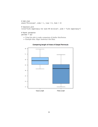
![# Comparing lengths (Sepal and Petal)
boxplot(iris[, c("Sepal.Length", "Petal.Length")], col = col)
title("Comparing length of Irises of Gaspe Peninsula")
# Comparing width (Sepal and Petal)
boxplot(iris[, c("Sepal.Width", "Petal.Width")], col = col)
title("Comparing width of Irises of Gaspe Peninsula")
• Sepal seems to be higher in terms of length and width than petal
• Will this pattern hold under different species?
30](https://image.slidesharecdn.com/r-training5-170404064141/85/R-training5-30-320.jpg)

![• Pattern still holds as Sepal width is higher than Petal width across all
species however, it’s interesting to see “setosa” is higher than the others.
# High level functions
boxplot(iris$Sepal.Length~iris$Species, col = col[1], ylim = c(min(iris$Petal.Length) - 0.1,
boxplot(iris$Petal.Length~iris$Species, col = 4, add = TRUE)
# Low level functions
legend("bottomright", c("Sepal", "Petal"), pch = 22, pt.bg = c(col[1], 4), title = "Iris Typ
title("Comparison of Iris Length by species", xlab = "Species", ylab = "Length")
# High level functions
boxplot(iris$Sepal.Width~iris$Species, col = col[1], ylim = c(min(iris$Petal.Width) - 0.1, m
boxplot(iris$Petal.Width~iris$Species, col = 4, add = TRUE)
# Low level functions
legend("bottomright", c("Sepal", "Petal"), pch = 22, pt.bg = c(col[1], 4), title = "Iris Typ
32](https://image.slidesharecdn.com/r-training5-170404064141/85/R-training5-32-320.jpg)

R training5
- 1. Introduction to Data Analysis and Graphics in R Introduction to Data Analysis and Graphics in R Hellen Gakuruh 2017-04-03 Slide 5: Graphics in R Outline What we will cover: • Introduction • High level plotting functions • Low level plotting functions • Interacting with graphics • Modifying a graph n • Plotting dichotomous and categorical variables • Plotting ordinal variables • Plotting continuous variables Introduction • R is renown for it’s plotting facilities; not only does it have all the well known graphs, it also offers an opportunity to build an entirely new type of graph • There three well known graphics in R; “base graphics”, “grid graphics (often implemented with package Lattice)” and “ggplot2” • On start-up, R initiates a graphical device; calls X11() IN UNIX, windows() in Windows and quartz() in mac • Plotting functions fall under three types of commands; High-level, Low- level, and Interactive 1
- 2. • Plots can be customized with “graphical parameters” High level plotting functions • They are designed to generate a complete plot with axes, labels and titles unless they are suppressed (with graphical parameters) • They start a new plot • Core R’s plotting function is plot() • plot() can produce a variety of different plots depending on type/class of first argument (hence, plot() is completely reliant on class(object)) Expected output of “plot()” • If only “x” is given only; – if it is a time series object (class = ts), a line plot is produced; other wise if it’s numeric a scatter plot of it’s index against it (x) is generated – if class(x) = "factor", a bar plot is produced – it’s an error when class(x) == "character" as plot needs a finite object to set a plotting window • If two variables are given and they are both numeric, output is a scatter plot Expected output of “plot()” • If a factor and a numeric vector are given, box plots are produced • If both vectors are factors, stacked bar plot is produced • If objected parsed is not a vector but a matrix, data frame or list, plot() will make plots per elements type • We produce a few of these as example using plain plot(obj) (without changing/giving other arguments) Time series object n ts <- ts(rnorm(12, 50), start = 1, end = 12, frequency = 1) class(ts) [1] "ts" n plot(ts) 2
- 3. Numeric vector n num <- rnorm(12, 50) class(num) [1] "numeric" n plot(num) 3
- 4. Factor vector n fac <- factor(sample(c("Y", "N"), 100, T, c(0.7, 0.3))) class(fac) [1] "factor" n plot(fac) 4
- 5. Two numeric vectors n num2 <- rnorm(12, 88) class(num2) [1] "numeric" n plot(num, num2) 5
- 6. Factor and numeric vector n set.seed(5) num3 <- rnorm(100, 88) class(num3) [1] "numeric" n plot(fac, num3) 6
- 7. Two factor vectors n fac2 <- factor(sample(c("F", "M"), 100, T, c(0.8, 0.2))) class(fac2) [1] "factor" n plot(fac, fac2) 7
- 8. Summary • In all these plots, axis, labels (except title) and in some, color is give, this makes them communicative • However, they might not be aesthetically up to requirements, this can be changed by passing other arguments including suppression of axis Other arguments to “plot” • Type of plot produced by plot() depends on first (and “y”) argument, but how it is generated depends on values parsed to other argument • Plot type can also be changed with argument “type”, though do this when sure it makes sense • “xlim” and “ylim” define x and y limits (min and max axis values), this can be changed especially if need a bit more padding 8
- 9. Other argument to “plot” function cont. • For customized axis like logs, argument “axes” can be suppressed • To annotate plot with additional graphical parameters, add them as argu- ment to high and low level plots or make a call to par(). . . more on this later (read ?par) Other High-level plots • hist() for histograms (univariate continuous distributions) • boxplot() for box-and-whiskers plot (for univariate numerical variables alone or categorised by a categorical variable) • barplot() for bar plots (for categorical distribution) • pie() for pie chart (for categorical distribution) Low level plotting functions • These functions add more information to an existing plot • Used to customize plots • Some of the most frequently used functions are; point(), lines(), text(), title(), abline(), polygon(), legend(), and axis() • We use some of these when plotting some of the example distributions Interacting with graphics • Interaction means extracting or adding information to a plot using a mouse (rather than inputting data to plot) • Two function for interaction in R are locator() and identify() • locator(n, type): one can select “n” number of points using left mouse button and if type is not specified, a list with two components x and y is outputted otherwise plotting over selected points given “type” is done • locator() is particularly handy in locating position for legends, and labels e.g. text(locator(1), "Outlier", adj=0) Interacting with graphics cont. • identify(x, y, labels) is used to highlight any of the points defined by x and y (using left mouse button) • These can be used to identify certain points and possibly label Demonstration on interacting with graphics 9
- 10. Graphical paramenters “par()” • Almost every aspect of a plot can be customized by graphical parameters • Graphical parameters come in “name=value” pair with all having a default value • Accessing current default parameters call par() for complete list • For a specific list call par detailing parameter of interest par("parameter") e.g. par("mfrow") • Changing any parameters can be done globally (not recommended) or individually Plotting dichotomous and categorical variables • Plotting of any distribution depends on whether it’s univariate (one vari- able), bi-variate (two variables) or multi-variate • Plots for univariate categorical variables (dichotomous included) are: – Pie charts (for few values e.g. 2) – Bar plots, and – Cleveland’s dot plots Plotting dichotomous and categorical variables conti. • Bi-variate plots – Stacked/besides bar plots – Four-fold display • Multi-variate plots – Mosaic – Four-fold plots Pie chart • Suitable when their few categories • Useful for showing “%’s” • Highly discouraged due to angular perception, in addition it uses a lot of ink 10
- 11. Pie chart example set.seed(5) response <- sample(c("Yes", "No"), 300, T, c(0.68, 0.32)) tab_response <- table(response) pie(tab_response, col = c("#99CCFF", "#6699CC")) labs <- paste0("(", round(as.vector(prop.table(tab_response)*100)), "%)") text(x = c(0.78, -0.50), y = c(0.80, -1), labels = c(labs[1], labs[2])) Bar plot • Consist of a sequence of rectangular bars with heights given by values given • Ideally, bars should be ordered by frequency rather than bar-label • Not recommended due to high-ink-ration (an alternative is Cleveland’s dot plot) 11
- 12. Bar plot cont. barplot(sort(tab_response, decreasing = TRUE), las = 1, col = c("#6699CC", "#99CCFF")) title("Bar chart", xlab = "Response", ylab = "Frequency") Cleveland’s dot plot • An alternative to bar chart (uses less data:ink ratio) • As an example, generate a “Cleveland’s dot plot” of the following data set and it should be: – titled “Total student’s trained by quarters (2016)” – have an x axis titled “Total student’s trained” – a sub-title “Data Mania Inc” (grey in color and slant), and – Y axis titled “Quarters”, balled according to (ordered) months given (March, Jun, Sep and Dec) – have blue colored points 12
- 13. Cleveland’s dot plot • Example data: Hypothetical random number of students trained by quarter totals for year 2016 set.seed(5) months <- sample(month.abb[c(3, 6, 9, 12)], size = 300, replace = TRUE) tab_months <- table(months)[c("Mar", "Jun", "Sep", "Dec")] tab_months months Mar Jun Sep Dec 81 78 60 81 Cleveland’s dot plot 13
- 14. n dotchart(as.numeric(tab_months), xlab = "Total student's Trained", ylab = "Quarters", bg = 4 title("Total students trained by quarters (2016)", sub = "Data Mania Inc.,", font.sub = 3, c axis(2, at = 1:4, labels = names(tab_months), las = 2) Bi-variate Stacked/Besides bar plots and Dot plot • Following earlier example, generate stacked/besides bar plot and bi-variate Cleveland’s dot plot • Adding second variable; Gender composition of students trained Bivariate stacked/besides bar plots and dot plot cont. set.seed(5) gender <- sample(c("Female", "Male"), 300, TRUE, c(0.7, 0.3)) monthgen_tab <- table(gender, months)[, c("Dec", "Sep", "Jun", "Mar")] monthgen_tab months gender Dec Sep Jun Mar Female 0 49 78 81 Male 81 11 0 0 14
- 15. Bivariate stacked/besides bar plots and dot plot cont. barplot(monthgen_tab, col = c("#6699CC", "#99CCFF"), beside = TRUE) legend("topright", legend = c("Female", "Male"), pch = 22 , pt.bg = c("#6699CC", "#99CCFF"), title("Student's trained by gender and month (2016)", xlab = "Month", ylab = "Number trained 15
- 16. Bivariate Cleveland’s dot plot dotchart(as.matrix(monthgen_tab)[, c("Mar", "Jun", "Sep", "Dec")], bg = 4, xlab = "Total num title("Total student's trained by gender and month", sub = "Data Mania Inc.", font.sub = 3, title(ylab = "Gender and month", line = 2.5) Four-fold plots • Used to display association (or lack of) • Designed for two binary variables (2 x 2 tables), this can be categorized by a third categorical variable with K levels (2 x 2 x k tables) • Association established if diagonal opposite cells in one direction tend to differ in size from those in the other direction • Color used to show this direction 16
- 17. Four-fold plots cont. • Rings around circle are confidence rings and if adjacent quadrants rings overlap then it corresponds to ( H_0: ) No association • Example data: R’s “Titanic” data (but only for passengers) # Convert Titanic data titanic_passengers <- colSums(Titanic[-4,,,]) titanic_passengers , , Survived = No Age Sex Child Adult Male 35 659 Female 17 106 , , Survived = Yes Age Sex Child Adult Male 29 146 Female 28 296 17
- 18. Four-fold for Titanic Passengers n # Plotting four fold plot fourfoldplot(titanic_passengers, std = "margins") • Plot shows association (rings do not overlap and diagonal opposite cells differ in size) between Titanic’s passenger’s age (child/adult) and gender (Male/Female) stratified by survival status (No/Yes) • Four-fold differ from pie chart as it varies radius while holding angle constant while pie varies angle while holding radius constant Mosaic plots • Originally proposed by Hartigan and Kleiner (1981, 1984) 18
- 19. • Similar to a divided bar plot where it displays counts of a contingency table directly by tiles whose area is proportional to the observed cell frequency • Later extended by Friendly (1992, 1994b) • Extended version generates greater visual impact by using color and shading to reflect size of residuals from independence (no association) • Used for exploratory data analysis (establish associations) and model building (display residuals of log-linear model) mosaicplot(titanic_passengers, color = TRUE) • Width of each column of tile in above figure is proportional to observed frequency of each cell and height of each tile is determined by conditional probabilities of row (age) in each column (sex). # Height of tiles prop.table(apply(titanic_passengers, 1:2, sum), 1) Age 19
- 20. Sex Child Adult Male 0.07364787 0.9263521 Female 0.10067114 0.8993289 Plotting continuous variables • Display will depend on whether it univariate, bi-variate or multivariate • Some often used displays for univariate: – Histograms – Density plots – Box-and-whisker plots – Dot plot – Stem-and-leave plot Plotting continuous variables • Some bi-variate displays – Scatter plot (both variables are continuous) – Box-and-whisker plot (one variable is continuous and the other cate- gorical) Histogram • Display distribution of observation in intervals called “bins” • Each bin is represented by a rectangle whose width is the intervals • Intervals can be equal through out (equidistant, R’s default) or not • Heights of each rectangle corresponds to number of observations falling within an interval (bin) • Generated with function “hist” or plot(x, type = “h”) • Hist constructs bins from argument “breaks” Histogram cont. • Breaks are breaking points for each interval or bin • Giving a vector without this argument is okay (R will compute them), but it’s usually good to change them to show best picture of distribution • Argument “nclass” (compatible with S) can also be used to get number of breaks needed • Histograms are excellent for data with numerous observations 20
- 21. Histogram cont. # Example data: Edgar Anderson's Iris Data sepal <- iris$Sepal.Length sepal [1] 5.1 4.9 4.7 4.6 5.0 5.4 4.6 5.0 4.4 4.9 5.4 4.8 4.8 4.3 5.8 5.7 5.4 [18] 5.1 5.7 5.1 5.4 5.1 4.6 5.1 4.8 5.0 5.0 5.2 5.2 4.7 4.8 5.4 5.2 5.5 [35] 4.9 5.0 5.5 4.9 4.4 5.1 5.0 4.5 4.4 5.0 5.1 4.8 5.1 4.6 5.3 5.0 7.0 [52] 6.4 6.9 5.5 6.5 5.7 6.3 4.9 6.6 5.2 5.0 5.9 6.0 6.1 5.6 6.7 5.6 5.8 [69] 6.2 5.6 5.9 6.1 6.3 6.1 6.4 6.6 6.8 6.7 6.0 5.7 5.5 5.5 5.8 6.0 5.4 [86] 6.0 6.7 6.3 5.6 5.5 5.5 6.1 5.8 5.0 5.6 5.7 5.7 6.2 5.1 5.7 6.3 5.8 [103] 7.1 6.3 6.5 7.6 4.9 7.3 6.7 7.2 6.5 6.4 6.8 5.7 5.8 6.4 6.5 7.7 7.7 [120] 6.0 6.9 5.6 7.7 6.3 6.7 7.2 6.2 6.1 6.4 7.2 7.4 7.9 6.4 6.3 6.1 7.7 [137] 6.3 6.4 6.0 6.9 6.7 6.9 5.8 6.8 6.7 6.7 6.3 6.5 6.2 5.9 21
- 22. Code used to plot op <- par("mfrow") par(mfrow = c(1, 2)) hist(sepal, col = "#99CCFF", ann = FALSE) title("Breaks = 10", xlab = "Sepal Length", ylab = "Frequency") hist(sepal, nclass = 15, col = "#6699cc", ann = FALSE) title("Breaks = 15", xlab = "Sepal Length", ylab = "Frequency") par(mfrow = op) Density Plots • Fit “smooth” curve by computing kernel density estimates • Based on probability theory 22
- 23. dens_sepal <- density(sepal) plot(dens_sepal, type = "n") polygon(dens_sepal, col = "#99CCFF") Box-and-whisker plot (univariate) • Used to visualize data distribution in terms of quarters • Shows outliers • Good comparison displays as multiple variables or groups can be plotted side-by-side states <- as.data.frame(state.x77[, c("Illiteracy", "Life Exp", "Murder", "HS Grad")]) 23
- 24. # Layout (1 row by 2 columns) op <- par("mfrow") par(mfrow = c(1, 2)) # Visualise distributions boxplot(states$Illiteracy, col = "#99CCFF") boxplot(states$'Life Exp', col = "#6699CC") # Reset original layout par(mfrow = op) • Both distributions have no outliers (points beyond whiskers) • First distribution has most of it’s values at the lower side suggesting a positive skewness (right tail) • Second distribution look almost symmetrical as lower and upper quarters look the same though it’s middle value is more on the lower side 24
- 25. Dot plots (Uni-variate) • An alternative to box plot when n (sample size) is small • They are one dimensional scatter plots • Called stripchart in R • Example data: 49.3, 48.1, 51.4, 48.1, 49, 49.3, 49.5, 49.8, 49.9, 50.4, 50.1 and 50.3 stripchart(round(num, 1), pch = 22, bg = col[1]) title("Dot plot for small sample size", xlab = "Observations") Stem-and-leave plot • Used to show distribution of observation • Use actual values rather than points 25
- 26. • Stem is the whole number and is plotted on the left side while on the right side (separated by a vertical bar) are the fractions # Example data (sorted) sort(round(num, 1)) [1] 48.1 48.1 49.0 49.3 49.3 49.5 49.8 49.9 50.1 50.3 50.4 51.4 # # Stem-and-leave plot stem(round(num, 1)) The decimal point is at the | 48 | 11 49 | 033589 50 | 134 51 | 4 Scatter plot • Used to show relationship between two continuous variables • Relationship is said to exist if points have a visible pattern (positive or negative) • No relationship exists if not pattern is visible; points are scattered plot(states[, 1:2], pch = 21, bg = col[1]) title("Association between Illiteracy and Life Expectancy") 26
- 27. n • Scatter plot shows some negative pattern suggesting an association between “Life Expectancy” and “Illiteracy” (cor = -0.5884779) Box-and-whisker plot (bi-variate) • Useful to display numerical variable by strata’s or groups of another categorical variable • Can also be used to compare two numerical distributions 27
- 28. # Box plot with slant axis op <- par("mar") par(mar = c(7, 4, 4, 2) + 0.1) # Plot without axis boxplot(states$`Life Exp`~state.division, col = col[1], xaxt = "n", xlab = "") # Add axis without labels axis(1, labels = FALSE) # Labels as levels of categorical variable labs <- levels(state.division) # Add labels text(1:length(labs), par("usr")[3] - 0.25, srt = 45, adj = 1, labels = labs, xpd = TRUE) 28
- 29. # Add xlab mtext("Divisions", side = 1, line = 6, font = 2) # Annotate plot title("Life expectancy for each US division", ylab = "Life expectancy") # Reset parameter par(mar = op) • Using box plot to make comparison of similar distribution • Example data: Elgar Anderson’s Iris Data 29
- 30. # Comparing lengths (Sepal and Petal) boxplot(iris[, c("Sepal.Length", "Petal.Length")], col = col) title("Comparing length of Irises of Gaspe Peninsula") # Comparing width (Sepal and Petal) boxplot(iris[, c("Sepal.Width", "Petal.Width")], col = col) title("Comparing width of Irises of Gaspe Peninsula") • Sepal seems to be higher in terms of length and width than petal • Will this pattern hold under different species? 30
- 31. • Pattern still holds, Sepal length is higher than Petal length across all species 31
- 32. • Pattern still holds as Sepal width is higher than Petal width across all species however, it’s interesting to see “setosa” is higher than the others. # High level functions boxplot(iris$Sepal.Length~iris$Species, col = col[1], ylim = c(min(iris$Petal.Length) - 0.1, boxplot(iris$Petal.Length~iris$Species, col = 4, add = TRUE) # Low level functions legend("bottomright", c("Sepal", "Petal"), pch = 22, pt.bg = c(col[1], 4), title = "Iris Typ title("Comparison of Iris Length by species", xlab = "Species", ylab = "Length") # High level functions boxplot(iris$Sepal.Width~iris$Species, col = col[1], ylim = c(min(iris$Petal.Width) - 0.1, m boxplot(iris$Petal.Width~iris$Species, col = 4, add = TRUE) # Low level functions legend("bottomright", c("Sepal", "Petal"), pch = 22, pt.bg = c(col[1], 4), title = "Iris Typ 32
- 33. title("Comparison of Iris Width by species", xlab = "Species", ylab = "Width") 33