Staad pro-getting started &tutorial
1 like2,943 views

The document provides information about installing and getting started with STAAD.Pro 2006 structural analysis software. It describes the system requirements, contents of the installation CD, installation process, copy protection device, and how to run STAAD.Pro and related programs like STAAD.etc, Sectionwizard, and STAAD.foundation. The installation process involves selecting the security system, installing desired programs and modules, and selecting default units. A copy protection device like a hardware lock is required to fully use the programs.


![Tutorial 11-56
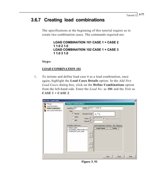
Creating load case 3
Load cases 1 and 2 were primary load cases. Load case 3 will be
defined as a load combination. So, the next step is to define load
case 3 as 0.75 x (Load 1 + Load 2), which is a load combination.
8. To do this, once again, highlight the Load Cases Details option. In
the Add New Load Cases dialog box, click on the Define
Combinations option from the left-hand side. Specify the Title as
75 Percent of [DL+LL+WL].
Figure 1. 55
In the Define Combinations box, the default load combination type
is set to be Normal, which means an algebraic combination. The
other combination types available are called SRSS (square root of
sum of squares) and ABS (Absolute). The SRSS type offers the
flexibility of part SRSS and part Algebraic. That is, some load
cases are combined using the square root of sum of squares
approach, and the result is combined with other cases algebraically,
as in
A + SQRT(B*B + C*C)
where A, B and C are the individual primary cases.
We intend to use the default algebraic combination type (Normal).](https://image.slidesharecdn.com/staad-pro-gettingstartedtutorial-150902114348-lva1-app6891/85/Staad-pro-getting-started-tutorial-96-320.jpg)


![Tutorial 1 1-67
2. A Load List dialog box comes up. From the Load Cases list box on
the left, double click on 1: DEAD + LIVE and 3: 75 Percent of
[DL+LL+WL] to send them to the Load List box on the right, as
shown below. Then click on the OK button to dismiss the dialog
box.
Figure 1. 67](https://image.slidesharecdn.com/staad-pro-gettingstartedtutorial-150902114348-lva1-app6891/85/Staad-pro-getting-started-tutorial-107-320.jpg)


![Tutorial 11-96
****************************************************
* *
* STAAD.Pro *
* Version Bld *
* Proprietary Program of *
* Research Engineers, Intl. *
* Date= *
* Time= *
* *
* USER ID: *
****************************************************
1. STAAD PLANE PORTAL FRAME
2. START JOB INFORMATION
3. ENGINEER DATE
4. END JOB INFORMATION
5. INPUT WIDTH 79
6. UNIT FEET KIP
7. JOINT COORDINATES
8. 1 0 0 0; 2 0 15 0; 3 20 15 0; 4 20 0 0
9. MEMBER INCIDENCES
10. 1 1 2; 2 2 3; 3 3 4
11. DEFINE MATERIAL START
12. ISOTROPIC STEEL
13. E 4.176E+006
14. POISSON 0.3
15. DENSITY 0.489024
16. ALPHA 6.5E-006
17. DAMP 0.03
18. END DEFINE MATERIAL
19. MEMBER PROPERTY AMERICAN
20. 1 3 TABLE ST W12X35
21. 2 TABLE ST W14X34
22. CONSTANTS
23. MATERIAL STEEL MEMB 1 TO 3
24. UNIT INCHES KIP
25. MEMBER OFFSET
26. 2 START 6 0 0
27. 2 END -6 0 0
28. SUPPORTS
29. 1 FIXED
30. 4 PINNED
31. UNIT FEET KIP
32. LOAD 1 DEAD + LIVE
33. MEMBER LOAD
34. 2 UNI GY -2.5
35. LOAD 2 WIND FROM LEFT
36. JOINT LOAD
37. 2 FX 10
38. LOAD COMB 3 75 PERCENT OF {DL+LL+WL]
39. 1 0.75 2 0.75
40. PERFORM ANALYSIS PRINT STATICS CHECK
P R O B L E M S T A T I S T I C S
-----------------------------------
NUMBER OF JOINTS/MEMBER+ELEMENTS/SUPPORTS = 4/ 3/ 2
ORIGINAL/FINAL BAND-WIDTH= 1/ 1/ 6 DOF
TOTAL PRIMARY LOAD CASES = 2, TOTAL DEGREES OF FREEDOM = 7
SIZE OF STIFFNESS MATRIX = 1 DOUBLE KILO-WORDS
REQRD/AVAIL. DISK SPACE = 12.0/ 3884.9 MB, EXMEM = 488.4 MB
STATIC LOAD/REACTION/EQUILIBRIUM SUMMARY FOR CASE NO. 1
DEAD + LIVE
***TOTAL APPLIED LOAD ( KIP FEET ) SUMMARY (LOADING 1 )
SUMMATION FORCE-X = 0.00
SUMMATION FORCE-Y = -47.50
SUMMATION FORCE-Z = 0.00
SUMMATION OF MOMENTS AROUND THE ORIGIN-
MX= 0.00 MY= 0.00 MZ= -475.00](https://image.slidesharecdn.com/staad-pro-gettingstartedtutorial-150902114348-lva1-app6891/85/Staad-pro-getting-started-tutorial-136-320.jpg)


![Tutorial 1 1-117
1.10.5 Changing the degree of freedom for
which forces diagram is plotted
Force and moment diagrams can be plotted for 6 degrees of
freedom – Axial, Shear-Y, Shear-Z, Torsion, Moment-Y, Moment-
Z. One may select or de-select one of more of these degrees of
freedom from View | Structure Diagrams | Loads and Results.
Let us select Shear yy and select load case 3 (75 PERCENT OF
[DL+LL+WL] as shown below.
Figure 1. 109](https://image.slidesharecdn.com/staad-pro-gettingstartedtutorial-150902114348-lva1-app6891/85/Staad-pro-getting-started-tutorial-157-320.jpg)


Staad pro-getting started &tutorial
- 1. STAAD.Pro 2006 GETTING STARTED AND TUTORIALS A Bentley Solutions Center www.reiworld.com www.bentley.com/staad
- 2. STAAD.Pro 2006 is a suite of proprietary computer programs of Research Engineers, a Bentley Solutions Center. Although every effort has been made to ensure the correctness of these programs, REI will not accept responsibility for any mistake, error or misrepresentation in or as a result of the usage of these programs. RELEASE 2006, Build 1005 © 2006 Bentley Systems, Incorporated. All Rights Reserved. Published July, 2007
- 3. About STAAD.Pro STAAD.Pro is a general purpose structural analysis and design program with applications primarily in the building industry - commercial buildings, bridges and highway structures, industrial structures, chemical plant structures, dams, retaining walls, turbine foundations, culverts and other embedded structures, etc. The program hence consists of the following facilities to enable this task. 1. Graphical model generation utilities as well as text editor based commands for creating the mathematical model. Beam and column members are represented using lines. Walls, slabs and panel type entities are represented using triangular and quadrilateral finite elements. Solid blocks are represented using brick elements. These utilities allow the user to create the geometry, assign properties, orient cross sections as desired, assign materials like steel, concrete, timber, aluminum, specify supports, apply loads explicitly as well as have the program generate loads, design parameters etc. 2. Analysis engines for performing linear elastic and pdelta analysis, finite element analysis, frequency extraction, and dynamic response (spectrum, time history, steady state, etc.). 3. Design engines for code checking and optimization of steel, aluminum and timber members. Reinforcement calculations for concrete beams, columns, slabs and shear walls. Design of shear and moment connections for steel members. 4. Result viewing, result verification and report generation tools for examining displacement diagrams, bending moment and shear force diagrams, beam, plate and solid stress contours, etc. 5. Peripheral tools for activities like import and export of data from and to other widely accepted formats, links with other popular softwares for niche areas like reinforced and prestressed concrete slab design, footing design, steel connection design, etc. 6. A library of exposed functions called OpenSTAAD which allows users to access STAAD.Pro’s internal functions and routines as well as its graphical commands to tap into STAAD’s database and link input and output data to third-party software written using languages like C, C++, VB, VBA, FORTRAN, Java, Delphi, etc. Thus, OpenSTAAD allows users to link in-house or third-party applications with STAAD.Pro.
- 4. About the STAAD.Pro Documentation The documentation for STAAD.Pro consists of a set of manuals as described below. These manuals are normally provided only in the electronic format, with perhaps some exceptions such as the Getting Started Manual which may be supplied as a printed book to first time and new-version buyers. All the manuals can be accessed from the Help facilities of STAAD.Pro. Users who wish to obtain a printed copy of the books may contact Research Engineers. REI also supplies the manuals in the PDF format at no cost for those who wish to print them on their own. See the back cover of this book for addresses and phone numbers. Getting Started and Tutorials : This manual contains information on the contents of the STAAD.Pro package, computer system requirements, installation process, copy protection issues and a description on how to run the programs in the package. Tutorials that provide detailed and step-by-step explanation on using the programs are also provided. Examples Manual This book offers examples of various problems that can be solved using the STAAD engine. The examples represent various structural analyses and design problems commonly encountered by structural engineers. Graphical Environment This document contains a detailed description of the Graphical User Interface (GUI) of STAAD.Pro. The topics covered include model generation, structural analysis and design, result verification, and report generation. Technical Reference Manual This manual deals with the theory behind the engineering calculations made by the STAAD engine. It also includes an explanation of the commands available in the STAAD command file. International Design Codes This document contains information on the various Concrete, Steel, and Aluminum design codes, of several countries, that are implemented in STAAD. The documentation for the STAAD.Pro Extension component(s) is available separately.
- 5. Part - I Getting Started System Requirements Installation Start-up
- 7. Table of Contents 1. Introduction 1 2. Hardware Requirements 2 3. Contents of the STAAD.Pro CD 4 4. Installation 6 5. Copy Protection Device 15 6. Running STAAD.Pro 17 7. Running STAAD.etc 19 8. Running Sectionwizard 20 9. Running STAAD.foundation 21 10. Running Mesher 22
- 9. 1 1. Introduction STAAD.Pro is an analysis and design software package for structural engineering. This manual is intended to guide users who are new to this software as well as experienced users who want specific information on the basics of using the program. Part-I of this manual describes the following: • Hardware Requirements • Contents of the STAAD.Pro CD • Installation • Copy Protection Device • Running STAAD.Pro Part II of this manual contains tutorials on using STAAD.Pro. The tutorials guide a user through the processes of: • Creating a structural model. This consists of generating the structural geometry, specifying member properties, material constants, loads, analysis and design specifications, etc. • Visualization and verification of the model geometry • Running the STAAD analysis engine to perform analysis and design • Verification of results - graphically and numerically • Report generation and printing • Inter-operability. In other words, using STAAD.Pro in conjunction with other programs created by REI, such as STAAD.etc.
- 10. System Requirements, Installation and Start-up 2 2. Hardware Requirements The following requirements are suggested minimums. Systems with increased capacity provide enhanced performance. • PC with Intel-Pentium or equivalent. • Graphics card and monitor with 1024x768 resolution, 256 color display (16 bit high color recommended). • 128 MB RAM or higher. • Windows NT 4.0 or higher operating system. Windows 95, Windows 98 & Windows Me are no longer supported. The program works best on Windows 2000 and XP operating systems. • Sufficient free space on the hard disk to hold the program and data files. The disk space requirement will vary depending on the modules you are installing. A typical minimum is 500MB free space. • A multi-media ready system with sound card and speakers is needed to run the tutorial movies and slide shows. Note: Additional RAM, disk space, and video memory will enhance the performance of STAAD.Pro. Starting with STAAD.Pro Version 2001, the size of structures that the program can handle has been increased significantly. As a result of this, the minimum amount of physical + virtual memory required by the program also has increased to over 600MB. Users may need to ensure that adequate amounts of virtual memory are available, and in Windows NT and 2000 systems, parameters such as paging file sizes should be large enough or span over multiple drives if the free space on any one drive runs low. Another issue to keep in mind is the location of the “TEMP” parameter as in the “SET TEMP” environment variable in Windows NT and 2000 systems. While performing calculations, depending on the structure size, the program may create gigantic scratch files which are placed in the folder location associated with
- 11. System Requirements, Installation and Start-up 3 the “TEMP” parameter. Users may wish to point the “SET TEMP” variable to a folder on a drive that has disk space sufficiently large to accommodate the requirements for large size structures. Note: The user must have a basic familiarity with Microsoft Windows systems in order to use the software.
- 12. System Requirements, Installation and Start-up 4 3. Contents of the STAAD.Pro CD Typically, a startup screen appears when the CD is placed in the drive. If it does not, you may initiate it by running SPROCD.EXE located at the root folder of the CD (This can be done by clicking on the file named SPROCD.EXE from Windows Explorer). The SPROCD Title screen appears as shown in Figure 1. Figure 1: The SPROCD Title Screen The choices offered by the Title screen are described below: Install STAAD Structural Suite This is the installation module containing the programs STAAD.Pro Version 2006, STAAD.etc, Sectionwizard and STAAD.foundation. STAAD.etc is a program that enables design of structural components such as base plates, bolt groups, cantilever retaining walls, rectangular footings, etc. Sectionwizard is a
- 13. System Requirements, Installation and Start-up 5 program for calculating properties such as area, moments of inertia, section modulii, torsional constants, etc., of various cross sections. STAAD.foundation is a program for designing reinforced concrete pile caps and pile groups, mat foundations, individual footings, etc. In order to use STAAD.etc, Sectionwizard and STAAD.foundation to their full capability, users must have purchased them as additional items of software. In the absence of a valid license to use them, those modules will work only in a demonstration mode. The installation procedure is explained in detail in the next section. View STAAD.Pro Manuals This takes the user to another screen which displays links to various STAAD.Pro manuals. Note: STAAD.beam is not a part of the STAAD.Pro family of products. You need to purchase it separately. Install STAAD.beam STAAD.beam is a utility type of program for designing simple steel beams. Its usefulness lies in its ease of use, and its ability to create reports of the detailed calculations that goes into the design of members per standard codes like AISC ASD and AISC LRFD. Exit Exits the SPROCD program. All online documentation that comes with the program is created in HTML format. These may be accessed using any Internet browser such as Microsoft’s Internet Explorer or Netscape Navigator. A set of multi-media movies which demonstrate the procedure for using STAAD.Pro are accessible after installing the program. They can be accessed from the Help menu of the main screen of the program. These too can be viewed using a web browser.
- 14. System Requirements, Installation and Start-up 6 4. Installation If you receive a document titled Installation Notes, it will supercede all other related instructions. Close all applications before installing STAAD.Pro. Typically, a startup screen appears when the CD is placed in the drive. If it does not, you may initiate it by running SPROCD.EXE located at the root folder of the CD (This can be done by clicking on the file named SPROCD.EXE from Windows Explorer). For an explanation of the different facilities offered by the SPROCD program, please refer to the previous section. Note: In Windows NT, Windows 2000, and Windows XP systems, you have to log in with administrative rights before commencing installation. To commence installation, select the option named Install STAAD Structural Suite. Standard installation procedure available with any software running on Microsoft Windows is followed and hence is self-explanatory.
- 15. System Requirements, Installation and Start-up 7 Users installing the commercial version of the program will encounter the following screen. Figure 2: Customer Information & Serial Number If an older version of STAAD.Pro has already been installed in the machine, the serial number information will show up automatically in this dialog box. If STAAD.Pro is being installed for the first time in the machine, the Serial number box will be blank. In that case, enter the serial number provided in the CD case. If you are under Bentley Select Contract, you will be asked to confirm that you will be using a Bentley SELECT License by checking the box titled ‘I am under Bentley Select Contract’. This will provide the serial number that is required for this method of security only.
- 16. System Requirements, Installation and Start-up 8 When this box is checked, the following confirmation message box will be displayed. Figure 2a: Customer Information One of the initial screens you will encounter is the one shown in Figure 3. It pertains to the type of software security system that you purchased with STAAD.Pro. SELECT XM system refers to Bentley’s SELECT Server based licensing system .A Local Security generally refers to a hardware lock, which is an adapter- like device that is placed on the parallel or USB port of your computer. It could also be a software based system (instead of a hardlock), in which case, it will be a software license which binds STAAD.Pro to the specific computer you are installing it on. Network Security refers to a system that supports simultaneous multiple-user access. A separate instruction document containing the steps for network installations is provided to users who have opted for this latter type. Please refer to the file "Quickstart.pdf" located in the CD for further description of these systems.
- 17. System Requirements, Installation and Start-up 9 Figure 3: Selection of security system type If you have purchased SELECT XM license for the products, please refer to Quick Start & Troubleshooting Guide to understand how to install and configure SELECT XM licenses. If you do not have SELECT XM license information, you can still choose the “SELECT XM License” option during installation. The program will run in Trial Mode for 15 days. You should complete the SELECT XM License configuration within that period.
- 18. System Requirements, Installation and Start-up 10 If you choose Local Security, you are asked to select the type of hardware lock supplied to you, or the software license if that is applicable. The name of the lock is engraved on the cover of the lock. Make sure the type of lock you choose from Figure 4 matches that name. This is absolutely necessary to ensure that the program functions to its full capacity. Please note that if you do not have a license for STAAD.etc, Sectionwizard and/or STAAD.foundation, they will work only in the Demonstration mode. Figure 4: Selection of Local Security type
- 19. System Requirements, Installation and Start-up 11 You may install the program in any folder of your choice. A default folder name is supplied to you. Figure 5: Selection of the Installation Folder
- 20. System Requirements, Installation and Start-up 12 The next dialog box seeks confirmation from you as to whether you wish to install all the programs shown in the list. Advanced Mesher is a standalone program for generating finite element meshes for panel type entities like walls and slabs and is available for those who want advanced meshing facilities besides those which are built into the STAAD.Pro software. OpenSTAAD is a library of functions which enables users to access input and output data from their STAAD.Pro projects for extraction into their own applications. While Advanced Mesher and OpenSTAAD are free utilities supplied along with STAAD.Pro, the remainder of the programs in the list require your copy-protection device/system to support those. If you do not wish to have any specific item(s) installed, uncheck the associated box. Figure 6: Selection of programs to install
- 21. System Requirements, Installation and Start-up 13 You also have to choose a default unit system. This is to ensure that the length and force units frequently used by you will be available upon entry into the program each time. This is known as the base unit system, and mainly affects the units in which results are displayed, as well as default values for certain quantities. Please refer to one of the tutorials for additional information on these. Of course, it is always possible for you to change the base unit system within the program, at run-time, as frequently as you please. Figure 7: Selection of Default Unit System for STAAD.Pro
- 22. System Requirements, Installation and Start-up 14 Towards the end of the installation process, a message resembling the one shown in Figure 8 will appear. It is pertinent only to users who have received this program as an upgrade from earlier versions of STAAD.Pro, and are already using a security device with those versions. For those users, their hardware lock also needs to be upgraded to enable it to work with STAAD.Pro 2006. That process is done electronically - called re-programming the lock - and there is no need to physically replace the lock (in most of the cases). Figure 8: Information regarding upgrade of lock After the installation is complete, please restart your machine for the changes to take effect.
- 23. System Requirements, Installation and Start-up 15 5. Copy Protection Device As explained in the previous section, a copy protection device in the form of a Select XM License, a hardware lock, or a software license, is required to run STAAD.Pro, STAAD.etc, STAAD.foundation and Sectionwizard. If you are using a hardware lock, it must be inserted in the parallel port of your computer and must remain there during the entire duration that you are in one of the programs. If any other device, such as printer cable, hardware lock for other software, etc., is attached to the parallel port, we recommend that you attach the STAAD.Pro / STAAD.etc hardware lock in front of such devices. In case you have multiple locks, and cannot stack them for any reason, REI can replace your parallel port type with a USB type of lock. The hardware lock is configured for the programs and modules that you have purchased. If you install one of the programs or modules that is not supported by the hardware lock, that component may not be accessible, or will be operable only as a Demonstration version. The hardware lock driver(s) are automatically installed during the installation process. For computers running on Windows NT, Windows 2000, or Windows XP, you must have administrative rights before installing the program to enable proper installation of the hardware lock driver files. As can be seen from the tutorials in the later sections of this book, STAAD.Pro consists of various modules, each designed to perform a certain type of task in the model generation, analysis and result verification process. Version 2006 requires the hardlock to be in place during the entire time that any and all of these tasks are being performed.
- 24. System Requirements, Installation and Start-up 16 In other words, from the moment you start the program till the moment you exit it, the lock has to be in place. If the lock is detached at any time in between, the program will stop running, and request that you re-attach the lock. In the event that you are unable to, it will provide the opportunity to save the work and exit the program. To resume your work, you will have to put the lock back in the port and re-start the program. Another important aspect to note is that if you are upgrading from an earlier version of STAAD.Pro such as 2000, 2001 or 2002, one of the following is applicable with regards to the lock: a. The upgrade package should contain a new lock which replaces your old lock. b. The upgrade package should contain information outlining how you can re-program your earlier lock so that it becomes compatible with STAAD.Pro 2006.
- 25. System Requirements, Installation and Start-up 17 6. Running STAAD.Pro Click on the STAAD.Pro icon from the STAAD.Pro 2006 program group. Figure 9: Starting STAAD.Pro
- 26. System Requirements, Installation and Start-up 18 The STAAD.Pro main screen appears as shown in below. Figure 10: The STAAD.Pro screen If you are a first time user who is unfamiliar with STAAD.Pro, we suggest that you go through the tutorials shown in Section II of this manual.
- 27. System Requirements, Installation and Start-up 19 7. Running STAAD.etc To launch the STAAD.etc program, click on the STAAD.etc icon. Figure 11: Starting STAAD.etc For help on using this program, we suggest that you go through the STAAD.etc Documentation accessible by clicking on its icon shown in the above figure.
- 28. System Requirements, Installation and Start-up 20 8. Running Sectionwizard To launch Sectionwizard, choose one of the programs from the Sectionwizard menu. Figure 12: Starting Sectionwizard For help on using this program, please go through Sectionwizard Help shown in the above figure.
- 29. System Requirements, Installation and Start-up 21 9. Running STAAD.foundation To launch STAAD.foundation, click on the STAAD.foundation icon. Figure 13: Starting STAAD.foundation For help on using this program, please go through the STAAD.foundation Documentation shown in the above figure.
- 30. System Requirements, Installation and Start-up 22 10. Running Mesher To launch Mesher, click on the Mesher icon. Figure 14: Starting Mesher Information on using this program is available from the Help menus of the program.
- 31. System Requirements, Installation and Start-up 23
- 32. System Requirements, Installation and Start-up 24
- 34. s
- 35. Table of Contents Introduction 1 1. Tutorial Problem 1: 2D Portal Frame 1-1 1.1 Methods of creating the model 1-2 1.2 Description of the Tutorial Problem 1-3 1.3 Starting the Program 1-5 1.4 Creating a New Structure 1-10 1.5 Creating the Model using the Graphical Interface 1-13 1.5.1 Generating the Model Geometry 1-16 1.5.2 Switching On Node And Beam Labels 1-23 1.5.3 Specifying Member Properties 1-26 1.5.4 Specifying Material Constants 1-32 1.5.5 Changing the Input Units of Length 1-33 1.5.6 Specifying Member Offsets 1-35 1.5.7 Printing Member Information in the Output File 1-40 1.5.8 Specifying Supports 1-43 1.5.9 Viewing the model in 3D 1-48 1.5.10 Specifying Loads 1-50 1.5.11 Specifying the Analysis Type 1-60 1.5.12 Specifying Post-Analysis Print Commands 1-62 1.5.13 Short-listing the Load Cases to be used in Steel Design 1-66 1.5.14 Specifying Steel Design Parameters 1-68 1.5.15 Re-specifying the Analysis Command 1-74 1.5.16 Re-specifying the Track Parameter 1-75 1.5.17 Specifying the Check Code Command 1-76 1.6 Viewing the Input Command File 1-79 1.7 Creating the Model using the Command File 1-82 1.8 Performing Analysis/Design 1-91 1.9 Viewing the Output File 1-94 1.10 Post-Processing 1-102 1.10.1 Going to the Post-Processing Mode 1-103 1.10.2 Annotating the Displacements 1-106 1.10.3 Displaying Force/Moment Diagrams 1-111 1.10.4 Annotating the Force/Moment Diagram 1-114 1.10.5 Changing the Degree of Freedom for which Forces Diagram is Plotted 1-117 1.10.6 Displaying the Dimensions of The Members 1-120
- 36. 2. Tutorial Problem 2: RC Framed Structure 2-1 2.1 Methods of creating the model 2-2 2.2 Description of the Tutorial Problem 2-3 2.3 Starting the Program 2-6 2.4 Creating a New Structure 2-11 2.5 Elements of the STAAD.Pro Screen 2-14 2.6 Building the STAAD.Pro Model 2-15 2.6.1 Generating the Model Geometry 2-16 2.6.2 Changing the Input Units of Length 2-28 2.6.3 Specifying Member Properties 2-30 2.6.4 Specifying Geometric Constants 2-36 2.6.5 Specifying Material Constants 2-38 2.6.6 Specifying Supports 2-41 2.6.7 Specifying Loads 2-46 2.6.8 Specifying the Analysis Type 2-63 2.6.9 Short-listing the load cases to be used in Concrete Design 2-65 2.6.10 Specifying Concrete Design Parameters 2-67 2.6.11 Specifying Design Commands 2-71 2.7 Viewing the Input Command File 2-74 2.8 Creating the Model using the Command File 2-77 2.9 Performing the Analysis and Design 2-85 2.10 Viewing the Output File 2-88 2.11 Post-Processing 2-96 2.11.1 Going to the Post-Processing Mode 2-97 2.11.2 Viewing the Deflection Diagram 2-99 2.11.3 Switching between load cases for viewing the deflection diagram 2-101 2.11.4 Changing the size of the deflection diagram 2-105 2.11.5 Annotating Displacements 2-108 2.11.6 Changing the units in which displacement values are annotated 2-111 2.11.7 The Node Displacement Table 2-114 2.11.8 Displaying Force/Moment Diagrams 2-119 2.11.9 Switching between load cases for viewing the Force/Moment diagram 2-122 2.11.10 Changing the size of the Force/Moment diagram 2-126 2.11.11 Changing the degree of freedom for which forces diagram is plotted 2-129 2.11.12 Annotating the Force/Moment diagram 2-131
- 37. 2.11.13 Changing the units in which Force/Moment values are annotated 2-134 2.11.14 Beam Forces Table 2-137 2.11.15 Viewing the Force/Moment diagrams from the Beam | Graphs Page 2-141 2.11.16 Restricting the load cases for which results are viewed 2-145 2.11.17 Using Member Query 2-147 2.11.18 Producing an on-screen Report 2-152 2.11.19 Taking Pictures 2-155 2.11.20 Creating Customized Reports 2-157 3. Tutorial Problem 3: Analysis of a slab 3-1 3.1 Methods of creating the model 3-2 3.2 Description of the tutorial problem 3-3 3.3 Starting the program 3-6 3.4 Creating a new structure 3-11 3.5 Elements of the STAAD.Pro screen 3-14 3.6 Building the STAAD.Pro model 3-15 3.6.1 Generating the model geometry 3-16 3.6.2 Changing the input units of length 3-53 3.6.3 Specifying Element Properties 3-55 3.6.4 Specifying Material Constants 3-61 3.6.5 Specifying Supports 3-62 3.6.6 Specifying Primary Load Cases 3-67 3.6.7 Creating Load Combinations 3-77 3.6.8 Specifying the analysis type 3-82 3.6.9 Specifying post-analysis print commands 3-85 3.7 Viewing the input command file 3-89 3.8 Creating the model using the command file 3-91 3.9 Performing the analysis and design 3-98 3.10 Viewing the output file 3-101 3.11 Post-Processing 3-109 3.11.1 Viewing stress values in a tabular form 3-110 3.11.2 Printing the tables 3-112 3.11.3 Changing the units of values which appear in the above tables 3-113 3.11.4 Limiting the load cases for which the results are displayed 3-115 3.11.5 Stress Contours 3-117 3.11.6 Animating stress contours 3-123 3.11.7 Creating AVI Files 3-124
- 38. 3.11.8 Viewing plate results using element query 3-127 3.11.9 Producing an onscreen report 3-131 3.11.10 Viewing Support Reactions 3-136 4. Tutorial Problem 4: Interoperability (using STAAD.Pro and STAAD.etc) 4-1 4.1 Understanding STAAD.etc 4-2 4.2 Description of the Tutorial Problem 4-3 4.3 Using the Interactive Mode in STAAD.Pro 4-4 4.4 Designing a Footing based on results from STAAD.Pro 4-9 4.5 Designing a Base Plate based on results from STAAD.Pro 4-15 4.7 Saving the Interactive Design as a STAAD.etc File 4-16 5. Frequently Performed Tasks FPT-1 1 Selecting nodes, beams, plates, etc. FPT-1 2 Viewing the structure from different angles FPT-8 3 Switching on labels for nodes, beams, plates, etc. FPT-12 4 Displaying a portion of the model by isolating it from the rest of the structure FPT-18 5 Creating Groups FPT-38 6 Displaying Loads on the screen FPT-47 7 Displaying Load Values on the screen FPT-52 8 Structural Tool Tip Options FPT-58 9 Identifying Beam Start and End FPT-62 10 Plotting from STAAD.Pro FPT-67
- 39. Introduction STAAD.Pro is a general purpose program for performing the analysis and design of a wide variety of types of structures. The basic three activities which are to be carried out to achieve that goal - a) model generation b) the calculations to obtain the analytical results c) result verification - are all facilitated by tools contained in the program's graphical environment. This manual contains four sample tutorials which guide the user through those 3 activities. The first of those tutorials demonstrates these processes using a simple two-dimensional steel portal frame. It is a good starting point for learning the program. If you are unfamiliar with STAAD.Pro, you will greatly benefit by going through this tutorial first. For the second tutorial, we have chosen a reinforced concrete frame. We generate the model, perform the analysis, and design the concrete beams and columns. It contains extensive details on the various facilities available for visualization and verification of results. The modelling and analysis of a slab is demonstrated in the third tutorial. Slabs, and other surface entities like walls are modelled using plate elements. Large surface entities may have to be defined using several elements and this sometimes requires a tool called a mesh generator. This tutorial shows the simple techniques as well as the mesh generation method for generating the finite element model of the slab. It also explains the methods by which one can check the results for plate elements. A tutorial which demonstrates the inter-operability features between STAAD.Pro and STAAD.etc. is presented in the fourth tutorial. STAAD.etc is a set of modules which can be used to perform component designs such as for a rectangular footing, base plate, cantilever retaining wall, moment connection, bolt group,
- 40. etc. Users who have purchased STAAD.etc in addition to STAAD.Pro may go through this tutorial to familiarize themselves with the process of utilizing STAAD.etc to perform secondary analysis and design tasks on a structure for which the primary analysis and design is done using STAAD.Pro.
- 41. 1-1 Tutorial Problem 1: 2D Portal Frame Section 1 This chapter provides a step-by-step tutorial for creating a 2D portal frame using STAAD.Pro. This tutorial covers the following topics. • Starting the Program • Creating a New Structure • Creating Joints and Members • Switching On Node and Beam Labels • Specifying Member Properties • Specifying Material Constants • Specifying Member Offsets • Printing Member Information • Specifying Supports • Specifying Loads • Specifying the Analysis Type • Specifying Post-Analysis Print Commands • Specifying Steel Design Parameters • Performing Analysis and Design • Viewing the Output File • Verifying results on screen – both graphically and numerically
- 42. Tutorial 11-2 1.1 Methods of creating the model There are two methods of creating the structure data: a. using the command file b. using the graphical model generation mode, or graphical user interface (GUI) as it is usually referred to. The Command File is a text file which contains the data for the structure being modeled. This file consists of simple English- language like commands. This command file may be created directly using the editor built into the program, or for that matter, any editor which saves data in text form, such as Notepad or WordPad available in Microsoft Windows. This command file is also automatically created behind the scenes when the structure is generated using the Graphical User Interface. The graphical model generation mode and the command file are seamlessly integrated. So, at any time, you may temporarily exit the graphical model generation mode and access the command file. You will find that it reflects all data entered through the graphical model generation mode. Further, when you make changes to the command file and save it, the GUI immediately reflects the changes made to the structure through the command file. Both methods of creating our model are explained in this tutorial. Section 1.3 through 1.6 explain the procedure for creating the file using the GUI. Section 1.7 describes creation of the command file using the STAAD.Pro text editor.
- 43. Tutorial 1 1-3 1.2 Description of the tutorial problem The structure for this project is a single bay, single story steel portal frame that will be analyzed and designed. The figure below shows the structure. 2 2 3 1 W12 x 35 15' - 0" 4 20' - 0" 1 2.5 KIP/FT 3 W12 x 35 W14 x 34 10 KIP Figure 1. 1 An input file called "Tut-01-portal.std" containing the input data for the above structure has been provided with the program. This file contains what would otherwise have resulted had we followed the procedure explained in Section 1.7.
- 44. Tutorial 11-4 BASIC DATA FOR THE STRUCTURE ATTRIBUTE DATA Member properties Members 1 & 3 : W12X35 Member 2 : W14X34 Material Constants Modulus of Elasticity : 29000 ksi Poisson's Ratio : 0.30 Member Offsets 6.0 inches along global X for member 2 at both ends Supports Node 1 : Fixed Node 4 : Pinned Loads Load case 1 : Dead + Live Beam 2 : 2.5 kips/ft downward along global Y Load case 2 : Wind From Left 10 kips point force at Node 2 Load case 3 : 75 Percent of (DL+LL+WL) Load Combination - L1 X 0.75 + L2 X 0.75 Analysis Type Linear Elastic (PERFORM) Steel Design Consider load cases 1 and 3 only. Parameters: Unsupported length of compression flange for bending : 10 ft for members 2 and 3, 15 ft for member 1. Steel Yield Stress : 40 ksi Perform member selection for members 2 and 3
- 45. Tutorial 1 1-5 1.3 Starting the program Select the STAAD.Pro icon from the STAAD.Pro 2006 program group. Figure 1. 2
- 46. Tutorial 11-6 The STAAD.Pro Graphical Environment will be invoked and the following screen comes up. Figure 1. 3 This New dialog box will come up every time we start the program. To turn this feature off, simply uncheck the Display this dialog box at the Startup box at the lower left hand corner. This feature can be turned on again at a later time when File | New is invoked from the main menu.
- 47. Tutorial 1 1-7 Note about the unit system : There are two base unit systems in the program which control the units (length, force, temperature, etc.) in which, values, specifically results and other information presented in the tables and reports, are displayed in. The base unit system also dictates what type of default values the program will use when attributes such as Modulus of Elasticity, Density, etc., are assigned based on material types – Steel, Concrete, Aluminum – selected from the program’s library (Please refer to Section 5 of the STAAD.Pro Technical Reference Manual for details). These two unit systems are English (Foot, Pound, etc.) and Metric (KN, Meter, etc.). If you recall, one of the choices made at the time of installing STAAD.Pro is this base unit system setting. That choice will serve as the default until we specifically change it. The place from where we can change this setting is under the File | Configure menu. To get to that option, first close down the dialog box shown in the earlier figure by clicking on Cancel. Then, click on the File | Configure menu option (see figure below) and choose the appropriate unit system you want. For this tutorial, let us choose the English units (Kip, Feet, etc.). Figure 1. 4
- 48. Tutorial 11-8 Figure 1. 5 Click on the Accept button to close the above dialog box.
- 49. Tutorial 1 1-9 Following this, select File | New once again. Figure 1. 6 The dialog box shown in Figure 1.3 will re-appear.
- 50. Tutorial 11-10 1.4 Creating a new structure 1. In the New dialog box, we provide some crucial initial data necessary for building the model. The structure type is to be defined by choosing from among Space, Plane, Floor and Truss. A Space type is one where the structure, the loading or both, cause the structure to deform in all 3 global axes (X, Y and Z). In a Plane type, the geometry, loading and deformation are restricted to the global X-Y plane only. A Floor type is a structure whose geometry is confined to the X-Z plane. A Truss type of structure carries loading by pure axial action. Truss members are deemed incapable of carrying shear, bending and torsion. For our model, let us choose Plane. We choose Foot as the length unit and Kilo Pound as the force unit in which we will start to build the model. The units can be changed later if necessary, at any stage of the model creation. We also need to provide a name in the File Name edit box. This is the name under which the structure data will be saved on the computer hard disk. The name “Structure?” (? will be a number) is recommended by the program by default, but we can change it to any name we want. Let us choose the name PORTAL. A default path name - the location on the computer drive where the file will be saved – is provided by the program under Location. If you wish to save the file in a different location, type in the name, or click the button and specify the desired path. After specifying the above input, click on the Next button.
- 51. Tutorial 1 1-11 Figure 1. 7 2. In the next dialog box, we choose the tools to be used to initially construct the model. Add Beam, Add Plate or Add Solid are, respectively, the starting points for constructing beams, plates or solids. Open Structure Wizard provides access to a library of structural templates which the program comes equipped with. Those template models can be extracted and modified parametrically to arrive at our model geometry or some of its parts. If the model is to be created initially using the STAAD command language, the Open STAAD Editor box can take us to the STAAD editor. Please remember that all these options are also available from the menus and dialog boxes of the GUI, even after we dismiss this dialog box. Note: If you wish to use the Editor to create the model, choose Open STAAD Editor, click Finish, and proceed to Section 1.7.
- 52. Tutorial 11-12 For our model, let us check the Add Beam option. Click on the Finish button. The dialog box will be dismissed and the STAAD.Pro graphical environment will be displayed. Figure 1. 8
- 53. Tutorial 1 1-13 1.5 Creating the model using the graphical user interface In order to generate the model graphically, we have to familiarize ourselves with the components of the STAAD.Pro screen. A sample of the STAAD.Pro screen is shown in Figure 1.9. The screen has five major elements as described below: Menu bar Located at the top of the screen, the Menu bar gives access to all the facilities of STAAD.Pro. Toolbar The dockable Toolbar gives access to the most frequently used commands. You may also create your own customized toolbar. Main Window This is the largest area at the center of the screen, where the model drawings and results are displayed in pictorial form. Page Control The Page Control is a set of tabs that appear on the left-most part of the screen. Each tab on the Page Control allows you to perform specific tasks. The organization of the Pages, from top to bottom, represents the logical sequence of operations, such as, definition of beams, specification of member properties, loading, and so on. Each tab has a name and an icon for easy identification. The name on the tabs may or may not appear depending on your screen resolution and the size of the STAAD.Pro window. However, the icons on the Page Control tabs always appear. The Pages in the Page Control area depend on the Mode of operation. The Mode of operation may be set from the Mode menu from the Menu bar.
- 54. Tutorial 11-14 Elements of the STAAD.Pro Screen Figure1.9
- 55. Tutorial 1 1-15 Data Area The right side of the screen is called the Data Area, where different dialog boxes, tables, list boxes, etc. appear depending on the type of operation you are performing. For example, when you select the Geometry | Beam Page, the Data Area contains the Node- Coordinate table and the Member-incidence table. When you are in the Load Page, the contents of the Data Area changes to display the currently assigned Load cases and the icons for different types of loads. The icons in the toolbar as well as in the Page Control area offer ToolTip help. As we move the mouse pointer over a button, the name of the button – called a ToolTip – appears above or below the button. This floating Tool tip help will identify the icon. A brief description of the icon also appears in the status bar. We are now ready to start building the model geometry. The steps and, wherever possible, the corresponding STAAD.Pro commands (the instructions which get written in the STAAD input file) are described in the following sections.
- 56. Tutorial 11-16 1.5.1 Generating the model geometry The structure geometry consists of joint numbers, their coordinates, member numbers, the member connectivity information, plate element numbers, etc. From the standpoint of the STAAD command file, the commands to be generated for the structure shown in section 1.2 are : JOINT COORDINATES 1 0. 0. ; 2 0. 15. ; 3 20. 15. ; 4 20. 0. MEMBER INCIDENCE 1 1 2 ; 2 2 3 ; 3 3 4 Steps: 1. We selected the Add Beam option earlier to facilitate adding beams to create the structure. This initiates a grid in the main drawing area as shown below. The directions of the global axes (X,Y,Z) are represented in the icon in the lower left hand corner of the drawing area. Figure 1. 10
- 57. Tutorial 1 1-17 2. A Snap Node/Beam dialog box also appears in the data area on the right side of the screen. The Linear tab is meant for placing the construction lines perpendicular to one another along a "left to right - top to bottom" pattern, as in the lines of a chess board. The Radial tab enables construction lines to appear in a spider-web style, which makes it is easy to create circular type models where members are modelled as piece-wise linear straight line segments. The Irregular tab can be used to create gridlines with unequal spacing that lie on the global planes or on an inclined plane. We will use the Linear tab. In our structure, the segment consisting of members 1 to 3, and nodes 1 to 4, happens to lie in the X-Y plane. So, in this dialog box, let us keep X-Y as the Plane of the grid. The size of the model that can be drawn at any time is controlled by the number of Construction Lines to the left and right of the origin of axes, and the Spacing between adjacent construction lines. By setting 20 as the number of lines to the right of the origin along X, 15 above the origin along Y, and a spacing of 1 feet between lines along both X and Y (see next figure) we can draw a frame 20ft X 15ft, adequate for our structure. Please note that these settings are only a starting grid setting, to enable us to start drawing the structure, and they do not restrict our overall model to those limits.
- 58. Tutorial 11-18 Figure 1. 11
- 59. Tutorial 1 1-19 3. To start creating the nodes, let us first activate the Snap Node/Beam button by clicking on it. Then, with the help of the mouse, click at the origin (0, 0) to create the first node. Figure 1. 12 4. In a similar fashion, click on the following points to create nodes and automatically join successive nodes by beam members. (0, 15), (20, 15), and (20, 0) The exact location of the mouse arrow can be monitored on the status bar located at the bottom of the window where the X, Y, and Z coordinates of the current cursor position are continuously updated.
- 60. Tutorial 11-20 When steps 1 to 4 are completed, the structure will be displayed in the drawing area as shown below. Figure 1. 13
- 61. Tutorial 1 1-21 5. At this point, let us remove the grid from the structure. To do that, click on the Close button in the Snap Node/Beam dialog box. Figure 1. 14
- 62. Tutorial 11-22 The grid will now be removed and the structure in the main window should resemble the figure shown below. Figure 1. 15 It is very important that we save our work often, to avoid loss of data and protect our investment of time and effort against power interruptions, system problems, or other unforeseen events. To save the file, pull down the File menu and select the Save command.
- 63. Tutorial 1 1-23 1.5.2 Switching on node and beam labels 1. Node and beam labels are a way of identifying the entities we have drawn on the screen. In order to display the node and beam numbers, right click anywhere in the drawing area. In the pop-up menu that comes up, choose Labels. Alternatively, one may access this option by selecting the View menu followed by the Structure Diagrams option from the top menu bar, and the Labels tab of the dialog box that comes up. Figure 1. 16
- 64. Tutorial 11-24 2. In the Diagrams dialog box that appears, turn the Node Numbers and Beam Numbers on and then click on OK. Figure 1. 17
- 65. Tutorial 1 1-25 The following figure illustrates the node and beam numbers displayed on the structure. The structure in the main window should resemble the figure shown below. Figure 1. 18 If you are feeling adventurous, here is a small exercise for you. Change the font of the node/beam labels by going to the View menu and selecting the Options command, and then selecting the appropriate tab (Node Labels / Beam labels) from the Options dialog box.
- 66. Tutorial 11-26 1.5.3 Specifying member properties Our next task is to assign cross section properties for the beams and columns (see figure in section 1.2). For those of us curious to know the equivalent commands in the STAAD command file, they are : MEMBER PROPERTY AMERICAN 1 3 TABLE ST W12X35 2 TABLE ST W14X34 Steps: 1. To define member properties, click on the Property Page icon located on the top toolbar. Figure 1. 19
- 67. Tutorial 1 1-27 Alternatively, one may go to the General | Property page from the left side of the screen as shown below. Figure 1. 20
- 68. Tutorial 11-28 2. In either case, the Properties dialog box comes up (see figure below). The property type we wish to create is the W shape from the AISC table. This is available under the Section Database button in the Properties dialog box as shown below. So, let us click on the Section Database button. Figure 1. 21
- 69. Tutorial 1 1-29 3. In the Section Profile Tables dialog box that comes up, select W Shape under the American option. Notice that the Material box is checked. Let us keep it that way because it will enable us to subsequently assign the material constants E, Density, Poisson, etc. along with the cross-section since we want to assign the default values. Choose W12X35 as the beam size, and ST as the section type. Then, click on the Add button as shown in the figure below. Detailed explanation of the terms such as ST, T, CM, TC, BC, etc. is available in Section 5 of the STAAD Technical Reference Manual. Figure 1. 22 4. To create the second member property (ST W14X34), select the W14X34 shape and click on the Add button. After the member properties have been created, let us Close the Section Profile Tables dialog box.
- 70. Tutorial 11-30 5. The next step is to associate the properties we just created with selected members in our model. Follow these steps. a. Select the first property reference in the Properties dialog box (W12X35). b. Make sure that the “Use Cursor to Assign” button is selected under the Assignment Method box. c. Click on the Assign button. The cursor changes to d. Using the cursor, click on members 1 and 3. e. Finally, click on the Assign button again, or click on the ‘Esc’ button on your keyboard to stop the assignment process. Figure 1. 23 6. In a similar fashion, assign the second property reference (W14X34) to member 2.
- 71. Tutorial 1 1-31 After both the properties have been assigned to the respective members, our model should resemble the following figure. Figure 1. 24 Let us once again save our structure by pulling down the File menu and selecting the Save command.
- 72. Tutorial 11-32 1.5.4 Specifying material constants In Section 1.5.3, we kept the Material check box “on” while assigning the member properties. Consequently, the material constants got assigned to the members along with the properties, and the following commands were generated in the command file: CONSTANTS E 29000 MEMB 1 TO 3 POISSON 0.3 MEMB 1 TO 3 DENSITY 0.000283 MEMB 1 TO 3 ALPHA 6.5e-006 MEMB 1 TO 3 Hence, there is no more a need to assign the constants separately. However, if we hadn’t assign them as before, we could go to the menu option Commands | Material Constants and assign them explicitly as shown in the figure below. Figure 1. 25
- 73. Tutorial 1 1-33 1.5.5 Changing the input units of length For specifying member offset values, as a matter of convenience, it is simpler if our length units are inches instead of feet. The commands to be generated are: UNIT INCHES KIP Steps: 1. To change the length units from feet to inch, click on the Input Units icon from the appropriate toolbar. Figure 1. 26 Alternatively, one may select the Tools | Set Current Input Unit menu option as shown in the next figure.
- 74. Tutorial 11-34 Figure 1. 27 2. In either case, the following dialog box comes up. Set the Length Units to Inch and click on the OK button. Figure 1. 28
- 75. Tutorial 1 1-35 1.5.6 Specifying member offsets Since beam 2 actually spans only the clear distance between the column faces, and not the center to center distance, we can take advantage of this aspect by specifying offsets. Member 2 is OFFSET at its START joint by 6 inches in the global X direction, 0.0 and 0.0 in Y and Z directions. The same member is offset by negative 6.0 inches at its END joint. The corresponding STAAD commands are: MEMBER OFFSET 2 START 6.0 0.0 0.0 2 END -6.0 0.0 0.0 Steps: 1. Since we know that member 2 is the one to be assigned with the offset, let us first select this member prior to defining the offset itself. Select member 2 by clicking on it using the Beams Cursor . The selected member will be highlighted. (Please refer to the ‘Frequently Performed Tasks’ section at the end of this manual to learn more about selecting members.) 2. To define member offsets, click on the Specification Page icon located in the top toolbar. Figure 1. 29
- 76. Tutorial 11-36 Alternatively, one may go to the General | Spec Page from the left side of the screen. Figure 1. 30
- 77. Tutorial 1 1-37 3. In either case, the Specifications dialog box shown below comes up. Member Releases and Offsets are defined through the Beam button in this dialog box as shown below. Figure 1. 31
- 78. Tutorial 11-38 4. In the Beam Specs dialog box that opens, select the Offset tab. We want to define the offset at the start node in the X direction. Hence, make sure that the Start option is selected under Location . Then, enter 6.0 in the X edit box. Since we have already selected the member, let us click on the Assign button. Figure 1. 32 5. To apply the offset at the end node, repeat steps 3 and 4, except for selecting the End option and providing -6.0 in the X edit box.
- 79. Tutorial 1 1-39 After both the Start and End offsets have been assigned, the model will look as shown below. Figure 1. 33 Click anywhere in the drawing area to un-highlight the member. Let us save the work again by pulling down the File menu and selecting the Save command.
- 80. Tutorial 11-40 1.5.7 Printing member information in the output file We would like to get a report consisting of information about all the members including start and end joint numbers (incidence), member length, beta angle and member end releases in the STAAD output file. The corresponding STAAD command is: PRINT MEMBER INFORMATION ALL Steps: 1. Since the information is required for all the members, select all the members by going to Select | By All | All Beams menu option. Figure 1. 34
- 81. Tutorial 1 1-41 2. Then, go to Commands | Pre Analysis Print | Member Information from the top menu bar as shown in the figure below. Figure 1. 35
- 82. Tutorial 11-42 3. Notice that the assignment method is set To Selection. Press the OK button in this dialog box. Figure 1. 36 Click anywhere in the drawing area to un-highlight the members. Let us also save our structure again by using the Save option of the File menu.
- 83. Tutorial 1 1-43 1.5.8 Specifying Supports The specifications of this problem (see section 1.2) call for restraining all degrees of freedom at node 1 (FIXED support) and a pinned type of restraint at node 4 (restrained against all translations, free for all rotations) The commands to be generated are : SUPPORTS 1 FIXED ; 4 PINNED Steps: 1. To create a support, click on the Support Page icon located in the top toolbar as shown below. Figure 1. 37
- 84. Tutorial 11-44 Alternatively, one may go to the General | Support Page from the left side of the screen. Figure 1. 38
- 85. Tutorial 1 1-45 2. In either case, the Supports dialog box comes up as shown in the next figure. Since we already know that node 1 is to be associated with a Fixed support, using the Nodes Cursor , select node 1. It becomes highlighted. (Please refer to the ‘Frequently Performed Tasks’ section at the end of this manual to learn more about selecting nodes.) 3. Then, click on the Create button in the Supports dialog box as shown below. Figure 1. 39
- 86. Tutorial 11-46 4. In the Create Support dialog box that opens, select the Fixed tab (which also happens to be the default) and click on the Assign button as shown below. This creates a FIXED type of support at node 1 where all 6 degrees of freedom are restrained. Figure 1. 40 5. To create a PINNED support at node 4, repeat steps 2 to 4, except for selecting node 4 and selecting the Pinned tab in the Create Support dialog box.
- 87. Tutorial 1 1-47 After the supports have been assigned, the structure will look like the one shown below. Figure 1. 41 After assigning both the supports, let us save our structure using the File | Save option.
- 88. Tutorial 11-48 1.5.9 Viewing the model in 3D Let us see how we can display our model in 3D. To do this, either right-click and select Structure Diagrams or go to View | Structure Diagrams menu. Figure 1. 42 In the ensuing dialog box, the Structure tab page allows you to set up structural view parameters as explained below. The options under 3D Sections control how the members are displayed. Selecting None displays the structure without displaying the cross-sectional properties of the members and elements. Selecting Full Sections displays the 3D cross-sections of members, depending on the member properties. Sections Outline displays only the outline of the cross-sections of members. Let us select Full Sections to draw the 3D sections. You can also change the color of the sections by clicking on the Section Outline color button under the Colors section. Then, click on OK.
- 89. Tutorial 1 1-49 Figure 1. 43 The resulting diagram is shown below. Figure 1. 44
- 90. Tutorial 11-50 1.5.10 Specifying Loads Three load cases are to be created for this structure. Details of the individual cases are explained at the beginning of this tutorial. The corresponding commands to be generated are listed below. UNIT FEET KIP LOADING 1 DEAD + LIVE MEMBER LOAD 2 UNI GY -2.5 LOADING 2 WIND FROM LEFT JOINT LOAD 2 FX 10. LOAD COMBINATION 3 75 PERCENT OF (DL+LL+WL) 1 0.75 2 0.75 Steps: The creation and assignment of load cases involves the following two steps: a. First, we will be creating all 3 load cases. b. Then, we will be assigning them to the respective members/nodes. Creating load cases 1 and 2 1. To create loads, first click on the Load Page icon located on the top tool bar. Figure 1. 45
- 91. Tutorial 1 1-51 Alternatively, one may go to the General | Load Page from the left side of the screen. Figure 1. 46 2. Before we create the first load case, we need to change our length units to feet. To do that, as before, utilize the Input Units icon (see section 1.5.5). Notice that a window titled “Load” appears on the right-hand side of the screen. To create the first load case, highlight Load Cases Details and then click on the Add button in the Load dialog box. Figure 1. 47
- 92. Tutorial 11-52 3. The Add New Load Cases dialog box comes up. The drop-down list box against Loading Type is available in case we wish to associate the load case we are creating with any of the ACI, AISC or IBC definitions of Dead, Live, Ice, etc. This type of association needs to be done if we intend to use the program's facility for automatically generating load combinations in accordance with those codes. Notice that there is a check box called Reducible per UBC/IBC. This feature becomes active only when the load case is assigned a Loading Type called Live at the time of creation of that case. Please refer to STAAD.Pro 2004 Release Report for further details. As we do not intend to use the automatic load combination generation option, we will leave the Loading Type as None. Enter DEAD + LIVE as the Title for Load Case 1 and click on the Add button. Figure 1. 48 The newly created load case will now appear under the Load Cases Details option. Figure 1. 49
- 93. Tutorial 1 1-53 To create the Member load, first highlight DEAD + LIVE. You will notice that the Add New Load Items dialog box shows more options now. Figure 1. 50 4. In the Add New Load Items dialog box, select the Uniform Force option under the Member Load item. Specify GY as the Direction, enter -2.5 as the Force and click on the Add button. Figure 1. 51
- 94. Tutorial 11-54 The next step is to create the second load case which contains a joint load. 5. Highlight Load Cases Details in the Load dialog box. In the Add New Load Cases dialog box, once again, we are not associating the load case we are about to create with any code based Loading Type and so, leave that box as None. Specify the Title of the second load case as WIND FROM LEFT and click on the Add button. Figure 1. 52 6. Next, to create the Joint load, highlight WIND FROM LEFT. Figure 1. 53
- 95. Tutorial 1 1-55 7. In the Add New Load Items dialog box, select the Node option under the Nodal Load item. Specify 10 for Fx, and click on the Add button. Figure 1. 54
- 96. Tutorial 11-56 Creating load case 3 Load cases 1 and 2 were primary load cases. Load case 3 will be defined as a load combination. So, the next step is to define load case 3 as 0.75 x (Load 1 + Load 2), which is a load combination. 8. To do this, once again, highlight the Load Cases Details option. In the Add New Load Cases dialog box, click on the Define Combinations option from the left-hand side. Specify the Title as 75 Percent of [DL+LL+WL]. Figure 1. 55 In the Define Combinations box, the default load combination type is set to be Normal, which means an algebraic combination. The other combination types available are called SRSS (square root of sum of squares) and ABS (Absolute). The SRSS type offers the flexibility of part SRSS and part Algebraic. That is, some load cases are combined using the square root of sum of squares approach, and the result is combined with other cases algebraically, as in A + SQRT(B*B + C*C) where A, B and C are the individual primary cases. We intend to use the default algebraic combination type (Normal).
- 97. Tutorial 1 1-57 9. In the Define Combinations box, select both load cases from the left side list box (by holding down the ‘Ctrl’ key) and click on the button. The load cases appear in the right side list box. Then, enter 0.75 in the Factor edit box. (These data indicate that we are adding the two load cases with a multiplication factor of 0.75 and that the load combination results would be obtained by algebraic summation of the results for individual load cases.) Press the Add button. Figure 1. 56 Now that we have completed the task of creating all 3 load cases, let us Close the Add New Load Cases dialog box.
- 98. Tutorial 11-58 Our next step is to associate load case 1 with member 2. Follow these steps. a. Select the first load reference in the Load dialog box (UNI GY -2.5 kip/ft). b. Make sure that the “Use Cursor to Assign” button is selected under the Assignment Method box. c. Click on the Assign button. The cursor changes to d. Using the cursor, click on member 2. e. Finally, click on the Assign button again, or type the ‘Esc’ button on your keyboard to stop the assignment process. Figure 1. 57
- 99. Tutorial 1 1-59 After the member load has been assigned, the model will look as shown below. Figure 1. 58 In a similar fashion, assign the second load case (FX 10 kip, ft) to Node 2. After assigning the joint load, the model will look as shown below. Figure 1. 59 Let us once again save our model by pulling down the File menu and selecting the Save command or by holding the ‘Ctrl’ key and pressing the ‘S’ key.
- 100. Tutorial 11-60 1.5.11 Specifying the analysis type The analysis type we are required to do is a linear static type. We also need to obtain a static equilibrium report. This requires the command: PERFORM ANALYSIS PRINT STATICS CHECK Steps: 1. To specify the Analysis command, go to Analysis/Print Page from the left side of the screen. By default, the Analysis sub-page from the second row is in focus as shown below. Figure 1. 60
- 101. Tutorial 1 1-61 2. In the Analysis/Print Commands dialog box that appears, make sure that the Perform Analysis tab is selected. Then, check the Statics Check print option. Finally, click on the Add button followed by the Close button. Figure 1. 61 Let us save the data once again using the File | Save option.
- 102. Tutorial 11-62 1.5.12 Specifying post-analysis print commands We would like to obtain the member end forces and support reactions written into the output file. This requires the specification of the following commands: PRINT MEMBER FORCES ALL PRINT SUPPORT REACTION LIST 1 4 Steps: 1. The dialog box for specifying the above commands is nested in the Post-Print sub-page of the Analysis/Print page. Figure 1. 62
- 103. Tutorial 1 1-63 2. Next, select all the members by rubber-banding around them using the mouse. 3. Click on the Define Commands button in the data area on the right hand side of the screen. Figure 1. 63
- 104. Tutorial 11-64 4. In the Analysis/Print Commands dialog box that appears, select the Member Forces tab and click on the Assign button followed by the Close button. Figure 1. 64 5. Repeat steps 2 to 4 except for selecting both the supports and selecting the Support Reactions tab in the Analysis/Print Commands dialog box. (Recall that the supports can be selected by turning the Nodes Cursor on, holding the ‘Ctrl’ key down, and clicking on the supports.) After clicking on the Assign button, Close the dialog box.
- 105. Tutorial 1 1-65 At this point, the Post Analysis Print dialog box should resemble the figure shown below. Figure 1. 65 Save the work using the File | Save menu option.
- 106. Tutorial 11-66 1.5.13 Short-listing the load cases to be used in steel design The steel design has to be performed for load cases 1 and 3 only per the specification at the beginning of this tutorial. To instruct the program to use just these cases, and ignore the remaining, we have to use the LOAD LIST command. The command will appear in the STAAD file as : LOAD LIST 1 3 Steps: 1. In the menus on the top of the screen, go to Commands | Loading | Load List option as shown below. Figure 1. 66
- 107. Tutorial 1 1-67 2. A Load List dialog box comes up. From the Load Cases list box on the left, double click on 1: DEAD + LIVE and 3: 75 Percent of [DL+LL+WL] to send them to the Load List box on the right, as shown below. Then click on the OK button to dismiss the dialog box. Figure 1. 67
- 108. Tutorial 11-68 1.5.14 Specifying steel design parameters The specifications listed in section 1.2 of this tutorial require us to provide values for some of the terms used in steel design because the default values of those terms are not suitable. The corresponding commands to be generated are: PARAMETER CODE AISC FYLD 5760 ALL UNT 10.0 MEMB 2 3 UNB 10.0 MEMB 23 TRACK 2 MEMB 2 3 SELECT MEMB 2 3 Steps: 1. To specify steel design parameters, go to Design | Steel Page from the left side of the screen. Make sure that under the Current Code selections on the top right hand side, AISC ASD is selected. Figure 1. 68
- 109. Tutorial 1 1-69 2. Click on the Define Parameters button in the Steel Design dialog box. Figure 1. 69 3. In the Design Parameters dialog box that comes up, select the FYLD option. Then, provide the Yield Strength as 5760 Kip/ft2 and click on the Add button. Figure 1. 70
- 110. Tutorial 11-70 4. To define the remaining parameters, repeat step 3 except for selecting the parameters and providing the values listed below. Parameter Value UNT 10 UNB 10 TRACK 2 5. When all the parameters have been added, click on the Close button in the Design Parameters dialog box. 6. The next step is to assign these parameters to specific members of the model. From looking at the requirements listed in the beginning of this tutorial, we know that the FYLD parameter is to be assigned to all the members, while the remaining parameters are to assigned to members 2 and 3. As before, use the Use Cursor to Assign method to assign these parameters. Figure 1. 71
- 111. Tutorial 1 1-71 After all the design parameters have been assigned, the Steel Design dialog box will look as shown below. Figure 1. 72
- 112. Tutorial 11-72 7. To specify the SELECT command, click on the Commands button in the Steel Design dialog box as shown below. The SELECT command is an instruction to the program to fetch and assign the least-weight cross-section which satisfies all the code requirements (PASSes) for the member. Figure 1. 73
- 113. Tutorial 1 1-73 8. In the Design Commands dialog box that appears, click on the SELECT option. Then, click on the Add button followed by the Close button. Figure 1. 74 9. Once again, we need to associate this command with members 2 and 3. You may either use the Use Cursor to Assign method or first select members 2 and 3 and then use the Assign to Selected Beams option. After the parameters are assigned, click anywhere in the drawing area to un-highlight the members. Let us save our structure by pulling down the File menu and selecting the Save command.
- 114. Tutorial 11-74 1.5.15 Re-specifying the analysis command When the analysis & design engine executes the member selection operation we specified in the previous step, a new set of properties will end up being assigned to those members. This has the effect of changing the stiffness distribution for the entire structure. Since the structure is statically indeterminate, we ought to re-analyze it if we want the nodal displacements, member forces, etc. to reflect this new stiffness distribution. The command to be generated is hence: PERFORM ANALYSIS Steps: 1. To specify the Analysis command, repeat step 1 of Section 1.5.11 of this tutorial. In the Analysis/Print Commands dialog box that comes up, select the Perform Analysis tab. Since we are not interested in a statics check report once again, let us check the No Print option. Finally, click on the Add button followed by the Close button. We should again save the work using File | Save.
- 115. Tutorial 1 1-75 1.5.16 Re-specifying the TRACK parameter The final calculation we need to do is make sure the current set of member properties pass the code requirements based on the up-to- date member forces. This will require that we do a code checking operation again. To restrict the output produced to a reasonable level, we specify the TRACK parameter again as: TRACK 1 ALL Steps: 1. To define and assign 1.0 for the TRACK parameter, repeat steps 1 to 4 of Section 1.5.14 of this tutorial. 2. Next, select all the members by rubber-banding around them using the mouse. (Please refer to the ‘Frequently Performed Tasks’ section at the end of this manual to learn more about selecting members.) Then, assign this parameter to all the members.
- 116. Tutorial 11-76 1.5.17 Re-specifying the CHECK CODE command The analysis operation carried out in response to the command in Section 1.5.15 will create a new set of member forces. These forces will very likely be quite different from those which were used in the member selection operation (see the commands of section 1.5.14). Consequently, we have to verify that the structure is safely able – from the standpoint of the design code requirements – to carry these new forces. A code checking operation, which uses the up-to-date cross sections of the members, and the latest member forces, will provide us with a status report on this issue. The command to be generated is hence: CHECK CODE ALL Steps: 1. If you have wandered away from the Steel Design page, from the Commands menu on top of the screen, select Design | Steel Design.
- 117. Tutorial 1 1-77 2. Click on the Commands button in the Steel Design dialog box as shown below. Figure 1. 75
- 118. Tutorial 11-78 3. In the Design Commands dialog box that appears, click on the Check Code tab. Then, click on the Add button followed by the Close button. Figure 1. 76 4. Since the CHECK CODE command has to be assigned to all the members, the easiest way to do that is to click on the Assign to View button. Figure 1. 77 We have now completed the tasks for assigning the input for this model. Let us save the file one last time using the File | Save option.
- 119. Tutorial 1 1-79 1.6 Viewing the input command file Steps: Let us now take a look at the data that has been written into the file that we just saved earlier. The contents of the file can be viewed either by clicking on the STAAD Editor icon or, by going to the Edit menu and choosing Edit Input Command File as shown below. Figure 1. 78 Figure 1. 79
- 120. Tutorial 11-80 A new window will open up with the data listed as shown here: Figure 1. 80 This window and the facilities it contains is known as the STAAD Editor.
- 121. Tutorial 1 1-81 We could make modifications to the data of our structure in this Editor if we wish to do so. Let us Exit the Editor without doing so by selecting the File | Exit menu option of the editor window (not the File | Exit menu of the main window behind the editor window). As we saw in Section 1.1, we could also have created the same model by typing the relevant STAAD commands into a text file using either the STAAD editor, or by using any external editor of our choice. If you would like to understand that method, proceed to the next section. If you want to skip that part, proceed to section 1.8 where we perform the analysis and design on this model.
- 122. Tutorial 11-82 1.7 Creating the model using the command file Let us now use the command file method to create the model for the above structure. The commands used in the command file are described later in this section. The STAAD.Pro command file may be created using the built-in editor, the procedure for which is explained further below in this section. Any standard text editor such as Notepad or WordPad may also be used to create the command file. However, the STAAD.Pro command file editor offers the advantage of syntax checking as we type the commands. The STAAD.Pro keywords, numeric data, comments, etc. are displayed in distinct colors in the STAAD.Pro editor. A typical editor screen is shown below to illustrate its general appearance. Figure 1. 81
- 123. Tutorial 1 1-83 To access the built-in editor, first start the program using the procedure explained in Section 1.3. Next, follow step 1 of Section 1.4. Figure 1. 82 You will then encounter the dialog box shown in the figure shown below. In that dialog box, choose Open STAAD Editor. Figure 1. 83
- 124. Tutorial 11-84 At this point, the editor screen similar to the one shown below will open. Figure 1. 84 Delete all the command lines displayed in the editor window and type the lines shown in bold below (You don’t have to delete the lines if you know which to keep and where to fill in the rest of the commands). The commands may be typed in upper or lower case letters. Usually the first three letters of a keyword are all that are needed -- the rest of the letters of the word are not required. The required letters are underlined. (“PLANE” = “PLA” = “plane” = “pla”)
- 125. Tutorial 1 1-85 STAAD PLANE PORTAL FRAME Every STAAD.Pro input file has to begin with the word STAAD. The word PLANE signifies that the structure is a plane frame (in the XY plane). The remainder of the words are the title of the problem, which is optional. If a line is typed with an asterisk in the first column, it signifies that the line is a comment line and should not be executed. For example, one could have put the optional title above on a separate line as follows. * PORTAL FRAME UNIT FEET KIP Specify the force and length units for the commands to follow. JOINT COORDINATES 1 0. 0. ; 2 0. 15. ; 3 20. 15. ; 4 20. 0. Joint numbers and their corresponding global X and Y coordinates are provided above. For example, 3 20 15. indicates that node 3 has an X coordinate of 20 ft and a Y coordinate of 15 ft. Note that the reason for not providing the Z coordinate is because the structure is a plane frame. If this were a space frame, the Z coordinate would also be required. Semicolons (;) are used as line separators. In other words, data which is normally put on multiple lines can be put on one line by separating them with a semicolon. MEMBER INCIDENCE 1 1 2 ; 2 2 3 ; 3 3 4 The members are defined by the joints to which they are connected.
- 126. Tutorial 11-86 MEMBER PROPERTY AMERICAN 1 3 TABLE ST W12X35 2 TABLE ST W14X34 Members 1 and 3 are assigned a W12X35 section from the built-in AMERICAN steel table. Member 2 has been assigned a W14X34. The word ST stands for standard single section. Sections 5.20.1 through 5.20.5 of the STAAD Technical Reference Manual explain the convention for assigning member property names. UNIT INCHES CONSTANTS E 29000.0 ALL POISSON 0.3 ALL The length unit is changed from FEET to INCHES to facilitate input of the modulus of elasticity (E). The keyword CONSTANT is required before material properties such as E, density, Poisson’s ratio, coefficient of thermal expansion (ALPHA) etc. can be provided. See Section 5.26 of the STAAD Technical Reference Manual for more information. MEMBER OFFSET 2 START 6.0 0. 0. 2 END -6.0 0. 0. The beam member is physically connected to the 2 columns at the face of the column, and not at the column centerline. This creates a rigid zone, about half the depth of the columns, at the 2 ends of the beam 2. This rigid zone is taken advantage of using member offsets (It is the user’s choice whether or not he/she wishes to use these). So, the above commands define that member 2 is eccentrically connected or OFFSET at its START joint by 6 inches in the global X direction, 0.0 and 0.0 in Y and Z directions. The same member is offset by negative 6.0 inches at its END joint. See Section 5.25 of the STAAD Technical Reference Manual for more information.
- 127. Tutorial 1 1-87 PRINT MEMBER INFORMATION ALL The above command is self-explanatory. The information that is printed includes start and end joint numbers (incidence), member length, beta angle and member end releases. SUPPORTS 1 FIXED ; 4 PINNED A fixed support is located at joint 1 and a pinned support (fixed for translations, released for rotations) at joint 4. More information on the support specification is available in Section 5.27 of the STAAD Technical Reference Manual. UNIT FT The length unit is changed to FEET to facilitate input of loads. LOADING 1 DEAD + LIVE MEMBER LOAD 2 UNI GY -2.5 The above commands identify a loading condition. DEAD + LIVE is an optional title to identify this load case. A UNIformly distributed MEMBER LOAD of 2.5 kips/ft is acting on member 2 in the negative global Y direction. Member Load specification is explained in Section 5.32 of the STAAD Technical Reference Manual. LOADING 2 WIND FROM LEFT JOINT LOAD 2 FX 10. The above commands identify a second load case. This load is a JOINT LOAD. A 10 kip force is acting at joint 2 in the global X direction.
- 128. Tutorial 11-88 LOAD COMBINATION 3 75 PERCENT OF (DL+LL+WL) 1 0.75 2 0.75 This command identifies a combination load with an optional title. The second line provides the components of the load combination case - primary load cases and the factors by which they should be individually multiplied. PERFORM ANALYSIS PRINT STATICS CHECK This command instructs the program to proceed with the analysis and produce a report of static equilibrium checks. Section 5.37 of the STAAD Technical Reference Manual offers information on the various analysis options available. PRINT MEMBER FORCES ALL PRINT SUPPORT REACTION LIST 1 4 The above print commands are self-explanatory. The member forces are in the member local axes while support reactions are in the global axes. LOAD LIST 1 3 PARAMETERS CODE AISC UNT 10.0 MEMB 2 3 UNB 10.0 MEMB 2 3 FYLD 5760 ALL TRACK 2.0 MEMB 2 3 SELECT MEMBER 2 3 The above sequence of commands is used to initiate the steel design process. The command PARAMETERS is followed by the various steel design parameters. Parameters are specified typically when their values differ from the built-in program defaults. Specifications of the AISC ASD code are to be followed. A parameter list for the AISC code is available in Table 3.1 of the Technical Reference Manual. ALL members have 10 ft unsupported length for the top and bottom flange (UNT and UNB). UNT and UNB are used to compute the allowable compressive stress in bending. The yield strength of steel is specified as 5760
- 129. Tutorial 1 1-89 ksf (40 ksi) since it is different from the default value of 36 ksi. The TRACK parameter controls the level of description of the output, 2.0 being the most detailed. The LOAD LIST command lists the load cases (1 and 3) to be used in the design. The SELECT MEMBER command asks the program to come up with the most economical section for members 2 and 3 in the context of the above analysis. PERFORM ANALYSIS When the analysis & design engine executes the member selection operation we specified in the previous step, a new set of properties will end up being assigned to those members. This has the effect of changing the stiffness distribution for the entire structure. Since the structure is statically indeterminate, we ought to re-analyze it if we want the nodal displacements, member forces, etc. to reflect this new stiffness distribution. The above command instructs the program to do another cycle of analysis. PARAMETER TRACK 1 ALL The TRACK parameter is re-specified. It controls the level of information produced in the steel design output. We have lowered it from 2.0 we specified earlier to 1.0 since we aren’t interested in the highest level of detail at this time. CHECK CODE ALL The analysis operation carried out earlier will create a new set of member forces. These forces will very likely be quite different from those which were used in the member selection operation. Consequently, we have to verify that the structure is safely able – from the standpoint of the design code requirements – to carry these new forces. A code checking operation, which uses the up-to- date cross sections of the members, and the latest member forces, will provide us with a status report on this issue. FINISH
- 130. Tutorial 11-90 A STAAD run is terminated using the FINISH command. Save the file and return to the main screen. This concludes the session on generating our model as a command file using the built-in editor. If you wish to perform the analysis and design, you may proceed to the next section of this manual. The on-screen post-processing facilities are explained in Section 1.10. (Remember that without successfully completing the analysis and design, the post-processing facilities will not be accessible.)
- 131. Tutorial 1 1-91 1.8 Performing Analysis/Design STAAD.Pro performs Analysis and Design simultaneously. In order to perform Analysis and Design, select the Run Analysis option from the Analyze menu. Figure 1. 85 If the structure has not been saved after the last change was made, you should save the structure first by using the Save command from the File menu. When you select the Run Analysis option from the Analyze menu, the following dialog box appears: Figure 1. 86 We are presented with the choice of 2 engines : the STAAD engine and the STARDYNE Advanced Analysis engine. The STARDYNE Analysis engine is suitable for advanced problems such as Buckling Analysis, Modal Extraction using various methods, etc. However, if the calculations call for steel or concrete design, UBC load generation, etc., we have to select the STAAD engine. So, let us ensure that the radio button is on the STAAD engine.
- 132. Tutorial 11-92 Click on the Run Analysis button. As the analysis progresses, several messages appear on the screen as shown in the figure below. Figure 1. 87 Notice that we can choose from the three options available in the above dialog box: Figure 1. 88
- 133. Tutorial 1 1-93 These options are indicative of what will happen after we click on the Done button. The View Output File option allows us to view the output file created by STAAD. The output file contains the numerical results produced in response to the various input commands we specified during the model generation process. It also tells us whether any errors were encountered, and if so, whether the analysis and design was successfully completed or not. Section 1.9 offers additional details on viewing and understanding the contents of the output file. The Go to Post Processing Mode option allows us to go to graphical part of the program known as the Post-processor. This is where one can extensively verify the results, view the results graphically, plot result diagrams, produce reports, etc. Section 1.10 explains the Post processing mode in greater detail. The Stay in Modelling Mode lets us continue to be in the Model generation mode of the program (the one we currently are in) in case we wish to make further changes to our model.
- 134. Tutorial 11-94 1.9 Viewing the output file During the analysis process, STAAD.Pro creates an Output file. This file provides important information on whether the analysis were performed properly. For example, if STAAD.Pro encounters an instability problem during the analysis process, it will be reported in the output file. We can access the output file using the method explained at the end of the previous section. Alternatively, we can select the File | View | Output File | STAAD Output option from the top menu. The STAAD.Pro output file for the problem we just ran is shown in the next few pages. Figure 1. 89
- 135. Tutorial 1 1-95 The STAAD.Pro output file is displayed through a file viewer called SproView. This viewer allows us to set the text font for the entire file and print the output file to a printer. Use the appropriate File menu option from the menu bar. Figure 1. 90 By default, the output file contains a listing of the entire Input also. You may choose not to print the echo of the Input commands in the Output file. Please select Commands | Miscellaneous | Set Echo option from the menu bar and select the Echo Off button. It is quite important that we browse through the entire output file and make sure that the results look reasonable, that there are no error messages or warnings reported, etc. Errors encountered during the analysis & design can disable access to the post- processing mode – the graphical screens where results can be viewed graphically. The information presented in the output file is a crucial indicator of whether or not the structure satisfies the engineering requirements of safety and serviceability.
- 136. Tutorial 11-96 **************************************************** * * * STAAD.Pro * * Version Bld * * Proprietary Program of * * Research Engineers, Intl. * * Date= * * Time= * * * * USER ID: * **************************************************** 1. STAAD PLANE PORTAL FRAME 2. START JOB INFORMATION 3. ENGINEER DATE 4. END JOB INFORMATION 5. INPUT WIDTH 79 6. UNIT FEET KIP 7. JOINT COORDINATES 8. 1 0 0 0; 2 0 15 0; 3 20 15 0; 4 20 0 0 9. MEMBER INCIDENCES 10. 1 1 2; 2 2 3; 3 3 4 11. DEFINE MATERIAL START 12. ISOTROPIC STEEL 13. E 4.176E+006 14. POISSON 0.3 15. DENSITY 0.489024 16. ALPHA 6.5E-006 17. DAMP 0.03 18. END DEFINE MATERIAL 19. MEMBER PROPERTY AMERICAN 20. 1 3 TABLE ST W12X35 21. 2 TABLE ST W14X34 22. CONSTANTS 23. MATERIAL STEEL MEMB 1 TO 3 24. UNIT INCHES KIP 25. MEMBER OFFSET 26. 2 START 6 0 0 27. 2 END -6 0 0 28. SUPPORTS 29. 1 FIXED 30. 4 PINNED 31. UNIT FEET KIP 32. LOAD 1 DEAD + LIVE 33. MEMBER LOAD 34. 2 UNI GY -2.5 35. LOAD 2 WIND FROM LEFT 36. JOINT LOAD 37. 2 FX 10 38. LOAD COMB 3 75 PERCENT OF {DL+LL+WL] 39. 1 0.75 2 0.75 40. PERFORM ANALYSIS PRINT STATICS CHECK P R O B L E M S T A T I S T I C S ----------------------------------- NUMBER OF JOINTS/MEMBER+ELEMENTS/SUPPORTS = 4/ 3/ 2 ORIGINAL/FINAL BAND-WIDTH= 1/ 1/ 6 DOF TOTAL PRIMARY LOAD CASES = 2, TOTAL DEGREES OF FREEDOM = 7 SIZE OF STIFFNESS MATRIX = 1 DOUBLE KILO-WORDS REQRD/AVAIL. DISK SPACE = 12.0/ 3884.9 MB, EXMEM = 488.4 MB STATIC LOAD/REACTION/EQUILIBRIUM SUMMARY FOR CASE NO. 1 DEAD + LIVE ***TOTAL APPLIED LOAD ( KIP FEET ) SUMMARY (LOADING 1 ) SUMMATION FORCE-X = 0.00 SUMMATION FORCE-Y = -47.50 SUMMATION FORCE-Z = 0.00 SUMMATION OF MOMENTS AROUND THE ORIGIN- MX= 0.00 MY= 0.00 MZ= -475.00
- 137. Tutorial 1 1-97 ***TOTAL REACTION LOAD( KIP FEET ) SUMMARY (LOADING 1 ) SUMMATION FORCE-X = 0.00 SUMMATION FORCE-Y = 47.50 SUMMATION FORCE-Z = 0.00 SUMMATION OF MOMENTS AROUND THE ORIGIN- MX= 0.00 MY= 0.00 MZ= 475.00 MAXIMUM DISPLACEMENTS ( INCH /RADIANS) (LOADING 1) MAXIMUMS AT NODE X = 1.82363E-01 2 Y = -1.46578E-02 3 Z = 0.00000E+00 0 RX= 0.00000E+00 0 RY= 0.00000E+00 0 RZ= -4.82525E-03 2 STATIC LOAD/REACTION/EQUILIBRIUM SUMMARY FOR CASE NO. 2 WIND FROM LEFT ***TOTAL APPLIED LOAD ( KIP FEET ) SUMMARY (LOADING 2 ) SUMMATION FORCE-X = 10.00 SUMMATION FORCE-Y = 0.00 SUMMATION FORCE-Z = 0.00 SUMMATION OF MOMENTS AROUND THE ORIGIN- MX= 0.00 MY= 0.00 MZ= -150.00 ***TOTAL REACTION LOAD( KIP FEET ) SUMMARY (LOADING 2 ) SUMMATION FORCE-X = -10.00 SUMMATION FORCE-Y = 0.00 SUMMATION FORCE-Z = 0.00 SUMMATION OF MOMENTS AROUND THE ORIGIN- MX= 0.00 MY= 0.00 MZ= 150.00 MAXIMUM DISPLACEMENTS ( INCH /RADIANS) (LOADING 2) MAXIMUMS AT NODE X = 7.27304E-01 2 Y = 2.47268E-03 2 Z = 0.00000E+00 0 RX= 0.00000E+00 0 RY= 0.00000E+00 0 RZ= -5.48842E-03 4 ************ END OF DATA FROM INTERNAL STORAGE ************ 41. UNIT INCHES KIP 42. PRINT MEMBER INFORMATION ALL MEMBER INFORMATION ------------------ MEMBER START END LENGTH BETA JOINT JOINT (INCH) (DEG) RELEASES 1 1 2 180.000 0.00 2 2 3 228.000 0.00 3 3 4 180.000 0.00 ************ END OF DATA FROM INTERNAL STORAGE ************
- 138. Tutorial 11-98 43. UNIT FEET KIP 44. PRINT MEMBER FORCES ALL MEMBER END FORCES STRUCTURE TYPE = PLANE ----------------- ALL UNITS ARE -- KIP FEET MEMBER LOAD JT AXIAL SHEAR-Y SHEAR-Z TORSION MOM-Y MOM-Z 1 1 1 23.18 -3.99 0.00 0.00 0.00 -11.48 2 -23.18 3.99 0.00 0.00 0.00 -48.40 2 1 -4.10 7.68 0.00 0.00 0.00 67.93 2 4.10 -7.68 0.00 0.00 0.00 47.32 3 1 14.30 2.77 0.00 0.00 0.00 42.34 2 -14.30 -2.77 0.00 0.00 0.00 -0.81 2 1 2 3.99 23.18 0.00 0.00 0.00 36.81 3 -3.99 24.32 0.00 0.00 0.00 -47.72 2 2 2.32 -4.10 0.00 0.00 0.00 -45.27 3 -2.32 4.10 0.00 0.00 0.00 -32.69 3 2 4.73 14.30 0.00 0.00 0.00 -6.34 3 -4.73 21.32 0.00 0.00 0.00 -60.31 3 1 3 24.32 3.99 0.00 0.00 0.00 59.88 4 -24.32 -3.99 0.00 0.00 0.00 0.00 2 3 4.10 2.32 0.00 0.00 0.00 34.74 4 -4.10 -2.32 0.00 0.00 0.00 0.00 3 3 21.32 4.73 0.00 0.00 0.00 70.97 4 -21.32 -4.73 0.00 0.00 0.00 0.00 ************** END OF LATEST ANALYSIS RESULT ************** 45. PRINT SUPPORT REACTION LIST 1 4 SUPPORT REACTIONS -UNIT KIP FEET STRUCTURE TYPE = PLANE ----------------- JOINT LOAD FORCE-X FORCE-Y FORCE-Z MOM-X MOM-Y MOM Z 1 1 3.99 23.18 0.00 0.00 0.00 -11.48 2 -7.68 -4.10 0.00 0.00 0.00 67.93 3 -2.77 14.30 0.00 0.00 0.00 42.34 4 1 -3.99 24.32 0.00 0.00 0.00 0.00 2 -2.32 4.10 0.00 0.00 0.00 0.00 3 -4.73 21.32 0.00 0.00 0.00 0.00 ************** END OF LATEST ANALYSIS RESULT ************** 46. LOAD LIST 1 3 47. PARAMETER 48. CODE AISC 49. FYLD 5760 MEMB 1 TO 3 50. UNT 10 MEMB 2 3 51. UNB 10 MEMB 2 3 52. TRACK 2 MEMB 2 3 53. SELECT MEMB 2 3
- 139. Tutorial 1 1-99 STAAD.PRO MEMBER SELECTION - (AISC 9TH EDITION) *********************************************** |--------------------------------------------------------------------------| | Y PROPERTIES | |************* | IN INCH UNIT | | * |=============================| ===|=== ------------ | |MEMBER 2 * | | | AX = 8.85 | | * | ST W14X30 | | --Z AY = 3.39 | |DESIGN CODE * | | | AZ = 3.47 | | AISC-1989 * =============================== ===|=== SY = 5.82 | | * SZ = 42.05 | | * |<---LENGTH (FT)= 19.00 --->| RY = 1.49 | |************* RZ = 5.73 | | | | 70.5 (KIP-FEET) | |PARAMETER | L1 L1 STRESSES | |IN KIP INCH | L1 IN KIP INCH | |--------------- + L3 -------------| | KL/R-Y= 153.21 | L3 FA = 6.36 | | KL/R-Z= 39.76 + fa = 0.45 | | UNL = 120.00 | L3 L1 FCZ = 21.68 | | CB = 1.00 +L1 FTZ = 24.00 | | CMY = 0.85 | L3 L3 FCY = 30.00 | | CMZ = 0.85 + FTY = 30.00 | | FYLD = 40.00 | L1 fbz = 20.13 | | NSF = 1.00 +---+---+---+---+---+---+---+---+---+---| fby = 0.00 | | DFF = 0.00 13.8 Fey = 6.36 | | dff = 0.00 ABSOLUTE MZ ENVELOPE Fez = 94.46 | | (WITH LOAD NO.) FV = 16.00 | | fv = 0.17 | | | | MAX FORCE/ MOMENT SUMMARY (KIP-FEET) | | ------------------------- | | | | AXIAL SHEAR-Y SHEAR-Z MOMENT-Y MOMENT-Z | | | | VALUE 4.7 24.3 0.0 0.0 70.5 | | LOCATION 0.0 19.0 0.0 0.0 9.5 | | LOADING 3 1 0 0 1 | | | |**************************************************************************| |* *| |* DESIGN SUMMARY (KIP-FEET) *| |* -------------- *| |* *| |* RESULT/ CRITICAL COND/ RATIO/ LOADING/ *| | FX MY MZ LOCATION | | ====================================================== | | PASS AISC- H1-3 0.999 1 | | 3.99 C 0.00 -70.55 9.50 | |* *| |**************************************************************************| | | |--------------------------------------------------------------------------|
- 140. Tutorial 11-100 STAAD.PRO MEMBER SELECTION - (AISC 9TH EDITION) *********************************************** |--------------------------------------------------------------------------| | Y PROPERTIES | |************* | IN INCH UNIT | | * |=============================| ===|=== ------------ | |MEMBER 3 * | | | AX = 10.00 | | * | ST W14X34 | | --Z AY = 3.61 | |DESIGN CODE * | | | AZ = 4.10 | | AISC-1989 * =============================== ===|=== SY = 6.91 | | * SZ = 48.64 | | * |<---LENGTH (FT)= 15.00 --->| RY = 1.53 | |************* RZ = 5.83 | | | | 71.0 (KIP-FEET) | |PARAMETER |L3 STRESSES | |IN KIP INCH | L3 IN KIP INCH | |--------------- + L3 L3 -------------| | KL/R-Y= 117.92 | L3 FA = 10.72 | | KL/R-Z= 30.87 + fa = 2.13 | | UNL = 120.00 | L3 L3 FCZ = 21.95 | | CB = 1.00 + FTZ = 24.00 | | CMY = 0.85 | L3 FCY = 30.00 | | CMZ = 0.85 + L3 L3 FTY = 30.00 | | FYLD = 40.00 | L0 fbz = 17.51 | | NSF = 1.00 +---+---+---+---+---+---+---+---+---+---| fby = 0.00 | | DFF = 0.00 -3.9 Fey = 10.74 | | dff = 0.00 ABSOLUTE MZ ENVELOPE Fez = 156.71 | | (WITH LOAD NO.) FV = 16.00 | | fv = 1.31 | | | | MAX FORCE/ MOMENT SUMMARY (KIP-FEET) | | ------------------------- | | | | AXIAL SHEAR-Y SHEAR-Z MOMENT-Y MOMENT-Z | | | | VALUE 24.3 4.7 0.0 0.0 71.0 | | LOCATION 0.0 0.0 0.0 0.0 0.0 | | LOADING 1 3 0 0 3 | | | |**************************************************************************| |* *| |* DESIGN SUMMARY (KIP-FEET) *| |* -------------- *| |* *| |* RESULT/ CRITICAL COND/ RATIO/ LOADING/ *| | FX MY MZ LOCATION | | ====================================================== | | PASS AISC- H1-2 0.886 3 | | 21.32 C 0.00 70.97 0.00 | |* *| |**************************************************************************| | | |--------------------------------------------------------------------------| 54. PERFORM ANALYSIS 55. PARAMETER 56. CODE AISC 57. TRACK 1 MEMB 1 TO 3 58. CHECK CODE MEMB 1 TO 3
- 141. Tutorial 1 1-101 STAAD.PRO CODE CHECKING - (AISC 9TH EDITION) ******************************************** ALL UNITS ARE - KIP FEET (UNLESS OTHERWISE NOTED) MEMBER TABLE RESULT/ CRITICAL COND/ RATIO/ LOADING/ FX MY MZ LOCATION ======================================================================= 1 ST W12X35 PASS AISC- H1-1 0.855 1 23.02 C 0.00 52.01 15.00 ----------------------------------------------------------------------- | MEM= 1, UNIT KIP-INCH, L= 180.0 AX= 10.30 SZ= 45.6 SY= 7.5 | | KL/R-Y= 116.7 CB= 1.00 YLD= 40.00 ALLOWABLE STRESSES: FCZ= 18.19 | | FTZ= 24.00 FCY= 30.00 FTY= 30.00 FC= 10.94 FT= 24.00 FV= 16.00 | ----------------------------------------------------------------------- 2 ST W14X30 PASS AISC- H1-3 0.969 3 5.16 C 0.00 66.64 19.00 ----------------------------------------------------------------------- | MEM= 2, UNIT KIP-INCH, L= 228.0 AX= 8.85 SZ= 42.1 SY= 5.8 | | KL/R-Y= 153.2 CB= 1.00 YLD= 40.00 ALLOWABLE STRESSES: FCZ= 21.68 | | FTZ= 24.00 FCY= 30.00 FTY= 30.00 FC= 6.36 FT= 24.00 FV= 16.00 | ----------------------------------------------------------------------- 3 ST W14X34 PASS AISC- H1-2 0.959 3 21.45 C 0.00 77.36 0.00 ----------------------------------------------------------------------- | MEM= 3, UNIT KIP-INCH, L= 180.0 AX= 10.00 SZ= 48.6 SY= 6.9 | | KL/R-Y= 117.9 CB= 1.00 YLD= 40.00 ALLOWABLE STRESSES: FCZ= 21.95 | | FTZ= 24.00 FCY= 30.00 FTY= 30.00 FC= 10.72 FT= 24.00 FV= 16.00 | ----------------------------------------------------------------------- 59. FINISH *********** END OF THE STAAD.Pro RUN *********** **** DATE= TIME= *** ************************************************************ * For questions on STAAD.Pro, please contact * * Research Engineers Offices at the following locations * * * * Telephone Email * * USA: +1 (714)974-2500 support@reiusa.com * * CANADA +1 (905)632-4771 detech@odandetech.com * * CANADA +1 (604)629 6087 staad@dowco.com * * UK +44(1454)207-000 support@reel.co.uk * * FRANCE +33(0)1 64551084 support@reel.co.uk * * GERMANY +49/931/40468-71 info@reig.de * * NORWAY +47 67 57 21 30 staad@edr.no * * SINGAPORE +65 6225-6015/16 support@reiasia.net * * INDIA +91(033)2357-3575 support@calcutta.reiusa.com * * JAPAN +81(03)5952-6500 eng-eye@crc.co.jp * * CHINA +86(411)363-1983 support@reiasia.net * * * * North America support@reiusa.com * * Europe support@reel.co.uk * * Asia support@reiasia.net * ************************************************************
- 142. Tutorial 11-102 1.10 Post-Processing STAAD.Pro offers extensive result verification and visualization facilities. These facilities are accessed from the Post Processing Mode. The Post Processing mode is used to verify the analysis and design results and generate reports. For this tutorial problem, we shall perform the following tasks: • Display deflection diagrams • Annotate Displacements • Display the force and moment diagrams. • Change the degree of freedom for which the force/moment diagram is plotted • Annotate the force diagram • Displaying dimensions of members
- 143. Tutorial 1 1-103 1.10.1 Going to the post-processing mode Steps: 1. At the end of section 1.8, we saw how one could go directly from the Analysis window to the post-processing screen. However, the formal method of accessing the Post Processing mode is either by clicking on the Post-Processing icon from the top toolbar or from the Mode menu as shown in the figures below. Figure 1. 91 Figure 1. 92
- 144. Tutorial 11-104 2. The Results Setup dialog box appears as shown below. Select the load cases for which to display the results. For this tutorial, let us select all the load cases. Then click on the OK button. Figure 1. 93
- 145. Tutorial 1 1-105 Notice that in the Post-Processing mode, the tabbed Page Control bar and the menu bar change to offer the post processing functions. Page Control in Page Control in Modeling Mode Post-Processing Mode Figure 1. 94 Menu Bar in Modeling Mode Menu Bar in Post-Processing Mode Figure 1. 95
- 146. Tutorial 11-106 1.10.2 Annotating the displacements Steps: The screen will now look like the figure shown below. Figure 1. 96 The diagram currently on display is the node deflection diagram for load case 1 (DEAD + LIVE). The title at the bottom of the diagram is indicative of that aspect. If you, say, wandered off into any other result diagram, and wanted to get back to the deflection diagram, just select the Node | Displacement tab along the page control area on the left side.
- 147. Tutorial 1 1-107 Figure 1. 97 Annotation is the process of displaying the displacement values on the screen. Select the View Value option from the Results menu. Figure 1. 98
- 148. Tutorial 11-108 The following dialog box comes up. From the Ranges tab, select All nodes. If you wish to annotate deflection for just a few nodes, specify the node numbers in the node list. Figure 1. 99 We will annotate the results for all the nodes. So, keep the button on All.
- 149. Tutorial 1 1-109 From the Node tab, check the Resultant option. Resultant stands for the square root of sum of squares of values of X,Y and Z displacements. Click the Annotate button and notice that the values appear on the structure. Click the Close button to close the dialog box. Figure 1. 100
- 150. Tutorial 11-110 The following figure shows the annotated deflection diagram for load case 1. Figure 1. 101
- 151. Tutorial 1 1-111 1.10.3 Displaying force/moment diagrams Steps: The simplest method to access the facilities for displaying force/moment diagrams is from the Beam | Forces page along the page control area on the left side of the screen. The bending moment MZ will be plotted by default, evidence of which can be found in the form of the Mz icon show in the diagram below which becomes active. Figure 1. 102
- 152. Tutorial 11-112 Figure 1. 103
- 153. Tutorial 1 1-113 The option for selecting the forces/moment diagram is available from another facility also - the Results | Bending Moment menu option. Figure 1. 104
- 154. Tutorial 11-114 1.10.4 Annotating the force/moment diagram Steps: Annotation is the process of displaying the force/moment values on the screen. Select the View Value option from the Results menu. Figure 1. 105 In the dialog box that comes up, click on the Ranges tab and select All members. If you wish to annotate the force/moment for just a few members, specify the beam numbers in the beam list.
- 155. Tutorial 1 1-115 Figure 1. 106 We will annotate the results for all members. So, keep the button on All. From the Beam Results tab, check the Ends and Mid Point options under the Bending section. Click the Annotate button and notice that the values appear on the structure. Click the Close button to close the dialog box. Figure 1. 107
- 156. Tutorial 11-116 The following figure shows the annotated MZ diagram for load case 2. Figure 1. 108
- 157. Tutorial 1 1-117 1.10.5 Changing the degree of freedom for which forces diagram is plotted Force and moment diagrams can be plotted for 6 degrees of freedom – Axial, Shear-Y, Shear-Z, Torsion, Moment-Y, Moment- Z. One may select or de-select one of more of these degrees of freedom from View | Structure Diagrams | Loads and Results. Let us select Shear yy and select load case 3 (75 PERCENT OF [DL+LL+WL] as shown below. Figure 1. 109
- 158. Tutorial 11-118 The resulting figure is shown below. Figure 1. 110 All degrees of freedom currently plotted will be indicated with a tick mark in the Diagrams dialog box. The icons of the Results toolbar may also be used to turn on/off specific degrees of freedom. Figure 1. 111
- 159. Tutorial 1 1-119 For the sake of easy identification, each degree of freedom (d.o.f) has been assigned a different color (see Diagrams dialog box shown above). One may change the color for that d.o.f. by clicking on the color button alongside the d.o.f, and make a new choice from the color palette. Figure 1. 112 The appearance of the diagram may also be set to one of the 3 – Hatch, Fill or Outline by turning on the relevant option in the dialog box shown earlier. Figure 1. 113
- 160. Tutorial 11-120 1.10.6 Displaying the dimensions of the members To display the dimension of the members, click on the Dimension icon. Alternatively, one may select the Dimension Beams option from the Tools menu. In the dialog box that opens, the option Dimension to View is active. Click on the Display button followed by the Close button, and the dimensions of the members will appear alongside the members. Figure 1. 114 Figure 1. 115
- 161. Tutorial 1 1-121 The diagram will look like the one shown below. Figure 1. 116 We can opt to save the screenshot by clicking on the Take Picture icon (shown below). This picture may be included in custom reports. See Chapter 2 for a tutorial on taking pictures as well as generating custom reports. Figure 1. 117
- 162. Tutorial 11-122 For obtaining a quick print of the plot on the screen, select the Print Current View icon as shown below. Figure 1. 118 For detailed information on the Post Processing features, please refer to the Post Processing section in the STAAD.Pro Graphical Environment manual.
- 163. Tutorial 1 1-123
- 164. 1-124
- 165. 2-1 Tutorial Problem 2: RC Framed Structure Section 2 This tutorial provides step-by-step instructions for creating the model of a reinforced concrete framed structure using STAAD.Pro. The following topics are covered : • Starting the Program • Creating Joints and Members • Switching On Node and Beam Labels • Specifying Member Properties and Material Constants • Specifying Member Orientation using Beta Angle • Specifying Supports • Specifying Loads • Specifying the Analysis Type • Specifying the parameters and instructions for Concrete Design • Performing Analysis and Design • Viewing results using the Output File • Viewing results on screen – both graphically and numerically • Producing customized reports
- 166. Tutorial 22-2 2.1 Methods of creating the model As explained in Section 1.1 of tutorial problem 1, there are two methods of creating the structure data: a) using the graphical model generation mode, or graphical user interface (GUI) as it is usually referred to. b) using the command file. Both methods are explained in this tutorial also. The graphical method is explained first, from Section 2.2 onwards. Section 2.8 describes the process of creating the model using the command file method and the STAAD.Pro text editor.
- 167. Tutorial 2 2-3 2.2 Description of the tutorial problem The structure for this project is a 2 bay, 2 story reinforced concrete frame. The figure below shows the structure. Our goal is to create the model, assign all required input, and perform the analysis and concrete design. 1 13.5m 4 5 2 3 6 2 5 3 4 6.0m 6.0m Z Y X Figure 2. 1
- 168. Tutorial 22-4 BASIC DATA FOR THE STRUCTURE ATTRIBUTE DATA Member properties Beams 2 & 5 : Rectangular, 275 mm width X 350 mm depth Columns 1 & 4 : Rectangular, 275 mm width X 300 mm depth Column 3 : Circular, 350 mm diameter Member Orientation All members except column 4 : Default Column 4 : Rotated by 90 degrees with respect to default condition Material Constants Modulus of Elasticity : 22 KN/sq.mm Density : 25 kn/cu.m Poisson's Ratio : 0.17 Supports Base of all columns : Fixed Loads Load case 1 : Dead Load Selfweight of the structure. Beams 2 & 5 : 400 kg/m in global Y downward Load case 2 : Live Load Beams 2 & 5 : 600 kg/m in global Y downward Load case 3 : Wind Load Beam 1 : 300 kg/m along positive global X Beam 4 : 500 kg/m along positive global X Load Case 4 : DEAD + LIVE L1 X 1.2 + L2 X 1.5 (Use REPEAT LOAD, not Load Combination) Load Case 5 : DEAD + WIND L1 X 1.1 + L2 X 1.3 (Use REPEAT LOAD, not Load Combination)
- 169. Tutorial 2 2-5 ATTRIBUTE DATA Analysis Type PDELTA Concrete Design Consider load cases 4 and 5 only. Parameters: Ultimate Strength of Steel : 415 N/sq.mm Concrete Strength : 25 N/sq.mm Clear cover for top : 25 mm Clear cover for bottom : 30 mm Clear cover for side : 25 mm Design beams 2 and 5 Design columns 1, 3 and 4
- 170. Tutorial 22-6 2.3 Starting the program Select the STAAD.Pro icon from the STAAD.Pro 2006 program group. Figure 2. 2
- 171. Tutorial 2 2-7 The STAAD.Pro Graphical Environment will be invoked and the following screen comes up. Figure 2. 3 This New dialog box will come up every time we start the program. To turn this feature off, simply uncheck the Display this dialog box at Startup box at the lower left hand corner. This feature can be turned on again at a later time when File | New is invoked from the main menu.
- 172. Tutorial 22-8 Note about the unit system : There are two base unit systems in the program which control the units (length, force, temperature, etc.) in which, values, specifically results and other information presented in the tables and reports, are displayed in. The base unit system also dictates what type of default values the program will use when attributes such as Modulus of Elasticity, Density, etc., are assigned based on material types – Steel, Concrete, Aluminum – selected from the program’s library (Please refer to Section 5 of the STAAD.Pro Technical Reference Manual for details). These two unit systems are English (Foot, Pound, etc.) and Metric (KN, Meter, etc.). If you recall, one of the choices made at the time of installing STAAD.Pro is this base unit system setting. That choice will serve as the default until we specifically change it. The place from where we can change this setting is under the File | Configure menu. To get to that option, first close down the dialog box shown in the earlier figure by clicking on Cancel. Then, click on the File | Configure menu option (see figure below) and choose the appropriate unit system you want. For this tutorial, let us choose the Metric units (KN, Meter, etc.). Figure 2. 4
- 173. Tutorial 2 2-9 Figure 2. 5 Click on the Accept button to close the above dialog box.
- 174. Tutorial 22-10 Following this, select File | New once again. Figure 2. 6 The dialog box shown in Figure 2.3 will re-appear.
- 175. Tutorial 2 2-11 2.4 Creating a new structure 1. In the New dialog box, we provide some crucial initial data necessary for building the model. The structure type is to be defined by choosing from among Space, Plane, Floor and Truss. A Space type is one where the structure, the loading or both, cause the structure to deform in all 3 global axes (X, Y and Z). In a Plane type, the geometry, loading and deformation are restricted to the global X-Y plane only. A Floor type is a structure whose geometry is confined to the X-Z plane. A Truss type of structure carries loading by pure axial action. Truss members are deemed incapable of carrying shear, bending and torsion. For our model, let us choose Space. We choose Meter as the length unit and Kilo Newton as the force unit in which we will start to build the model. The units can be changed later if necessary, at any stage of the model creation. We also need to provide a name in the File Name edit box. This is the name under which the structure data will be saved on the computer hard disk. The name “Structure?” (? will be a number) is recommended by the program by default, but we can change it to any name we want. Let us choose the name rcframe. A default path name - the location on the computer drive where the file will be saved – is provided by the program under Location. If you wish to save the file in a different location, type in the name, or click the button and specify the desired path. After specifying the above input, click on the Next button.
- 176. Tutorial 22-12 Figure 2. 7 2. In the next dialog box, we choose the tools to be used to initially construct the model. Add Beams, Add Plates or Add Solids are, respectively, the starting points for constructing beams, plates or solids. Open Structure Wizard provides access to a library of structural templates which the program comes equipped with. Those template models can be extracted and modified parametrically to arrive at our model geometry or some of its parts. If the model is to be created initially using the STAAD command language, the Open STAAD Editor box can take us to the STAAD editor. Please remember that all these options are also available from the menus and dialog boxes of the GUI, even after we dismiss this dialog box. Note: If you wish to use the Editor to create the model, choose Open STAAD Editor, click Finish, and proceed to Section 2.8.
- 177. Tutorial 2 2-13 For our model, let us check the Add Beam option. Click on the Finish button. The dialog box will be dismissed and the STAAD.Pro graphical environment will be displayed. Figure 2. 8
- 178. Tutorial 22-14 2.5 Elements of the STAAD.Pro screen The STAAD.Pro main window is the primary screen from where the model generation process takes place. It is important to familiarize ourselves with the components of that window before we embark on creating the RC Frame. Section 1.5 in tutorial problem 1 of this manual explains the components of that window in detail.
- 179. Tutorial 2 2-15 2.6 Building the STAAD.Pro model We are now ready to start building the model geometry. The steps and, wherever possible, the corresponding STAAD.Pro commands (the instructions which get written in the STAAD input file) are described in the following sections.
- 180. Tutorial 22-16 2.6.1 Generating the model geometry The structure geometry consists of joint numbers, their coordinates, member numbers, the member connectivity information, plate element numbers, etc. From the standpoint of the STAAD command file, the commands to be generated for the structure shown in section 2.2 are : JOINT COORDINATES 1 0.0 0.0 0.0 ; 2 0.0 3.5 0.0 3 6.0 3.5 0.0 ; 4 6.0 0.0 0.0 5 6.0 0.0 6.0 ; 6 6.0 3.5 6.0 MEMBER INCIDENCE 1 1 2 ; 2 2 3 ; 3 3 4 ; 4 5 6 ; 5 3 6 Steps: 1. We selected the Add Beam option earlier to enable us to add beams and columns to create the structure. This initiates a grid in the main drawing area as shown below. The directions of the global axes (X, Y, Z) are represented in the icon in the lower left hand corner of the drawing area. Figure 2. 9
- 181. Tutorial 2 2-17 2. A Snap Node/Beam dialog box also appears in the data area on the right side of the screen. In our structure, the segment consisting of members 1 to 3, and nodes 1 to 4, happens to lie in the X-Y plane. So, in this dialog box, let us keep X-Y as the Plane of the grid. The size of the model that can be drawn at any time is controlled by the number of Construction Lines to the left and right of the origin of axes, and the Spacing between adjacent construction lines. By setting 12 as the number of lines to the right of the origin along X, 7 above the origin along Y, and a spacing of 0.5 meter between lines along both X and Y (see figure below) we can draw a frame 6m X 3.5m, adequate for our segment. Please note that these settings are only a starting grid setting, to enable us to start drawing the structure, and they do not restrict our overall model to those limits. Figure 2. 10
- 182. Tutorial 22-18 3. To start creating the nodes, let us first activate the Snap Node/Beam button by clicking on it. Then, with the help of the mouse, click at the origin (0, 0) to create the first node. Figure 2. 11 4. In a similar fashion, click on the following points to create nodes and automatically join successive nodes by beam members. (0, 3.5), (6, 3.5) and (6, 0) The exact location of the mouse arrow can be monitored on the status bar located at the bottom of the window where the X, Y, and Z coordinates of the current cursor position are continuously updated.
- 183. Tutorial 2 2-19 When steps 1 to 4 are completed, the frame will be displayed in the drawing area as shown below. Figure 2. 12
- 184. Tutorial 22-20 5. At this point, let us remove the grid display from the structure. To do that, click on the Close button in the Snap Node/Beam dialog box. Figure 2. 13
- 185. Tutorial 2 2-21 The grid will now be removed and the structure in the main window should resemble the figure shown below. Figure 2. 14 6. It is very important that we save our work often, to avoid loss of data and protect our investment of time and effort against power interruptions, system problems, or other unforeseen events. To save the file, pull down the File menu and select the Save command.
- 186. Tutorial 22-22 Switching on node and beam labels 7. Node and beam labels are a way of identifying the entities we have drawn on the screen. In order to display the node and beam numbers, right click anywhere in the drawing area. In the pop-up menu that appears, choose Labels. Alternatively, one may access this option by selecting the View menu followed by the Structure Diagrams option from the top menu bar, and the Labels tab of the dialog box that comes up. Figure 2. 15
- 187. Tutorial 2 2-23 8. In the Diagrams dialog box that appears, turn the Node Numbers and Beam Numbers on and then click on OK. Figure 2. 16
- 188. Tutorial 22-24 The following figure illustrates the node and beam numbers displayed on the structure. The structure in the main window should resemble the figure shown below. Figure 2. 17 If you are feeling adventurous, here is a small exercise for you. Change the font of the node/beam labels by going to the View menu and selecting the Options command, and then selecting the appropriate tab (Node Labels / Beam labels) from the Options dialog box.
- 189. Tutorial 2 2-25 9. Examining the structure shown in section 2.2 of this tutorial, it can be seen that members 4 and 5 can be easily generated if we could first create a copy of members 1 and 2 and then rotate those copied units about a vertical line passing through the point (6, 0, 0, that is, node 4) by 90 degrees. Fortunately, such a facility does exist which can be executed in a single step. It is called Circular Repeat and is available under the Geometry menu. First, select members 1 and 2 using the Beams Cursor . (Please refer to the ‘Frequently Performed Tasks’ section at the end of this manual to learn more about selecting members.) 10. Then, either click on the Circular Repeat icon from the appropriate toolbar, or, go to the Geometry | Circular Repeat menu option as shown below. Figure 2. 18
- 190. Tutorial 22-26 11. In the 3D Circular dialog box that comes up, specify the Axis of Rotation as Y, Total Angle as 90 degrees, No. of Steps as 1 and the vertical line as passing through Node 4. Instead of specifying as passing through Node 4, one may also specify the X and Z co- ordinates as 6 and 0 respectively. Leave the Link Steps box unchecked and click on the OK button. Figure 2. 19
- 191. Tutorial 2 2-27 After completing the circular repeat procedure, the model will look as shown below. Before Figure 2. 20 After Figure 2. 21 If any of the members are presently selected, let us unselect them by clicking anywhere else in the drawing area. Then, let us once again save the work by pulling down the File menu and selecting the Save command.
- 192. Tutorial 22-28 2.6.2 Changing the input units of length As a matter of convenience, for specifying member properties for our structure, it is simpler if our length units are millimeter instead of meter. This will require changing the current length units of input. The commands to be generated are: UNIT MMS KN Steps: 1. Click on the Input Units icon from the appropriate toolbar. Figure 2. 22 Alternatively, one may select the Tools | Set Current Input Unit menu option as shown in the next figure.
- 193. Tutorial 2 2-29 Figure 2. 23 2. In either case, the following dialog box comes up. Set the Length Units to Millimeter and click on the OK button. Figure 2. 24
- 194. Tutorial 22-30 2.6.3 Specifying member properties Our next task is to assign cross section properties for the beams and columns (see section 2.2). For those of us curious to know the equivalent commands in the STAAD command file, they are : MEMB PROP 1 4 PRIS YD 300 ZD 275 2 5 PRIS YD 350 ZD 275 3 PRIS YD 350 Steps: 1. Click on the Property Page icon located on the Structure Tools toolbar. Figure 2. 25
- 195. Tutorial 2 2-31 Alternatively, one may go to the General | Property page from the left side of the screen as shown below. Figure 2. 26
- 196. Tutorial 22-32 2. In either case, the Properties dialog box comes up. The property type we wish to assign is called PRISMATIC, and is available under the Define button in the Properties dialog box as shown below. Figure 2. 27 3. In the dialog box that comes up, select the Rectangle tab. Notice that the field called Material is presently on the checked mode. If we keep it that way, the material properties of concrete (E, Poisson, Density, Alpha, etc.) will be assigned along with the cross-section name. The material property values so assigned will be the program defaults. We do not want default values, instead we will assign our own values later on. Consequently, let us uncheck the Material box. Then, enter the following values: YD = 300mm ZD = 275mm
- 197. Tutorial 2 2-33 Finally, click on the Add button as shown below. Figure 2. 28 4. To create the second member property (PRIS YD 350 ZD 275), provide 350 for YD and 275 for ZD (instead of 300 and 275) and click on the Add button. To create the third member property, in the Property dialog box, select the Circle option. Specify the diameter (YD) as 350 mm. Once again, uncheck the Material box and click on the Add button. Figure 2. 29 Now that we have finished creating the member properties, let us Close this dialog box.
- 198. Tutorial 22-34 The next step is to assign these member properties in the following manner: Rect 0.30x0.28 – members 1 and 4 Rect 0.35x0.28 – members 2 and 5 Cir 0.35 – member 3 To assign the member properties, follow these steps: a. Select the first property reference in the Properties dialog box (Rect 0.30x28). b. Make sure that the “Use Cursor to Assign” button is selected under the Assignment Method box. c. Click on the Assign button. The cursor changes to d. Using the cursor, click on members 1 and 4. e. Finally, click on the Assign button again, or type the ‘Esc’ button on your keyboard to stop the assignment process. Figure 2. 30 In a similar fashion, assign the remaining properties.
- 199. Tutorial 2 2-35 After all the member properties have been assigned, the model will look as shown below. Figure 2. 31 We ought to save the model once again by pulling down the File menu and selecting the Save command.
- 200. Tutorial 22-36 2.6.4 Specifying geometric constants In the absence of any explicit instructions, STAAD will orient the beams and columns of the structure in a pre-defined way. Orientation refers to the directions along which the width and depth of the cross section are aligned with respect to the global axis system. The rules which dictate this default orientation are explained in Section 1 of the STAAD.Pro Technical Reference Manual. We wish to orient member 4 so that its longer edges (sides parallel to local Y axis) are parallel to the global Z axis. This requires applying a beta angle of 90 degrees. The command which needs to be generated is : BETA 90 MEMB 4 Steps: 1. Select the Beta Angle tab in the Properties dialog box. 2. Click on the Create Beta Angle button. In the ensuing dialog box, specify the angle as 90 degrees. Select member 4 using the Beams Cursor . Notice that as we select the member, the Assignment Method automatically sets to Assign to Selected Beams. Click on the Assign button. Click anywhere in the drawing area to un-highlight the member.
- 201. Tutorial 2 2-37 Figure 2. 32 (An alternative method to assign beta angles is the following. First select the member for which you wish to assign the beta angle. Then, go to the Commands | Geometric Constants | Beta Angle menu option. Specify the Angle in Degrees to be 90, ensure that the assignment method is “To Selection” and click on OK. ) Figure 2. 33 One may view the orientation of the member local axes by going to the View | Structure diagrams | Labels menu option and switching on Beam Orientation.
- 202. Tutorial 22-38 2.6.5 Specifying material constants At the time of assigning member properties, we deliberately chose not to assign the material constants simultaneously, since we wanted to specify values which are different from the built-in defaults. The desired values are listed at the beginning of this tutorial. The corresponding commands we wish to generate in the STAAD input file are: CONSTANTS E 22 ALL UNIT METER DENSITY 25.0 ALL POISSON 0.17 ALL Steps: 1. From the Commands menu, select Material Constants. To define the Modulus of Elasticity, select the Elasticity option as shown below. Figure 2. 34
- 203. Tutorial 2 2-39 2. In the Material Constant dialog box that appears, enter 22 in the Enter Value box. Since the value has to be assigned to all the members of the structure, the current setting of the assignment method, namely, To View, allows us to achieve this easily. Then, click on OK. Figure 2. 35 3. For specifying the DENSITY constant, it will be convenient if we change our length units to meters. To change the length units, as before, click on the Input Units icon from the Structure toolbar, or select the Tools | Set Current Input Unit menu option from the top menu bar. In the Set Current Input Units dialog box that comes up, specify the length units as Meter. Figure 2. 36
- 204. Tutorial 22-40 4. Following the steps 1 and 2 above, we choose Commands | Material Constants | Density, specify the value as 25KN/m3 , and assign To View. 5. To define the POISSON’S RATIO, using the similar procedure as described above, provide the value 0.17 to all members in the View.
- 205. Tutorial 2 2-41 2.6.6 Specifying Supports The base nodes of all the columns are restrained against translation and rotation about all the 3 global axes (see section 2.2). In other words, fixed supports are to be specified at those nodes. The commands to be generated are : SUPPORTS 1 4 5 FIXED Steps: 1. To create supports, click on the Support Page icon located in the Structure Tools toolbar as shown below. Figure 2. 37
- 206. Tutorial 22-42 Alternatively, one may go to the General | Support Page from the left side of the screen. Figure 2. 38
- 207. Tutorial 2 2-43 2. In either case, the Supports dialog box comes up. Since we already know that nodes 1, 4 and 5 are to be associated with the Fixed support, using the Nodes Cursor , select these nodes. 3. Then, click on the Create button in the Supports dialog box as shown below. Figure 2. 39
- 208. Tutorial 22-44 4. The Create Support dialog box comes up. In the dialog box, the Fixed tab happens to be the default which is convenient for this case. Click on the Assign button as shown below. Figure 2. 40
- 209. Tutorial 2 2-45 After the supports have been assigned, the structure will look like the one shown below. Figure 2. 41 Click anywhere in the drawing area to un-select all selected nodes and prevent accidental assignment of unwanted data to those nodes. As earlier, save the work completed so far by going to the File menu and clicking on the Save command.
- 210. Tutorial 22-46 2.6.7 Specifying Loads 5 load cases are to be created for this structure. Details of the individual cases are explained at the beginning of this tutorial. The corresponding commands to be generated are listed below. Notice that cases 4 and 5 are to be generated not as the standard combination type, but using a combination load type called REPEAT LOAD. The instructions at the beginning of this tutorial require us to analyze this structure using an analysis type called PDelta. A Pdelta analysis is a non-linear type of analysis. In STAAD, to accurately account for the PDelta effects arising from the simultaneous action of previously defined horizontal and vertical loads, those previous cases must be included as components of the combination case using the REPEAT LOAD type. UNIT METER KG LOAD 1 DEAD LOAD SELFWEIGHT Y -1 MEMBER LOAD 2 5 UNI GY -400 LOAD 2 LIVE LOAD MEMBER LOAD 2 5 UNI GY -600 LOAD 3 WIND LOAD MEMBER LOAD 1 UNI GX 300 4 UNI GX 500 LOAD 4 DEAD + LIVE REPEAT LOAD 1 1.2 2 1.5
- 211. Tutorial 2 2-47 LOAD 5 DEAD + WIND REPEAT LOAD 1 1.1 3 1.3 Steps: LOAD CASE 1 1. To create loads, click on the Load Page icon located on the Structure Tools tool bar. Figure 2. 42 Alternatively, one may go to the General | Load Page from the left side of the screen. Figure 2. 43
- 212. Tutorial 22-48 2. A window titled “Load” appears on the right-hand side of the screen. To initiate the first load case, highlight the Load Cases Details option and click on the Add button. Figure 2. 44 3. The Add New Load Cases dialog box comes up. The drop-down list box against Loading Type is available in case we wish to associate the load case we are creating with any of the ACI, AISC or IBC definitions of Dead, Live, Ice, etc. This type of association needs to be done if we intend to use the program's facility for automatically generating load combinations in accordance with those codes. Notice that there is a check box called Reducible per UBC/IBC. This feature becomes active only when the load case is assigned a Loading Type called Live at the time of creation of that case. Please refer to STAAD.Pro 2004 Release Report for further details. As we do not intend to use the automatic load combination generation option, we will leave the Loading Type as None. Enter DEAD LOAD as the Title for Load Case 1 and click on Add.
- 213. Tutorial 2 2-49 Figure 2. 45 The newly created load case will now appear under the Load Cases Details option. Figure 2. 46
- 214. Tutorial 22-50 4. To generate and assign the selfweight load type, first highlight DEAD LOAD. You will notice that the Add New Load Items dialog box shows more options now. Figure 2. 47 5. In the Add New Load Items dialog box, select the Selfweight Load option under the Selfweight item. Specify the Direction as Y, and the Factor as -1.0. The negative number signifies that the selfweight load acts opposite to the positive direction of the global axis (Y in this case) along which it is applied. Click on the Add button. The selfweight load is applicable to every member of the structure, and cannot be applied on a selected list of members. Figure 2. 48
- 215. Tutorial 2 2-51 6. Load 1 contains an additional load component, the member loads on members 2 and 5. However, notice that the load values are listed in the beginning of this tutorial in kg and meter units. Rather than convert those values to the current input units, we will conform to those units. The current input units, which we last set while specifying Density, are KN and METER. We have to change the force unit to Kilogram. STAAD has a limitation in that one cannot change the units while editing load cases. If we attempt to, the following message will be displayed. Figure 2. 49 Click on OK. Close the Add New Load Items dialog box. Then, go to the Setup Page as shown below (or any other page). Figure 2. 50
- 216. Tutorial 22-52 As before, click on the Input Units icon from the top toolbar, or select the Tools | Set Current Input Unit menu option from the top menu bar. In the Set Current Input Units dialog box that comes up, specify the force units as Kilogram. Again, click on General | Load page to resume creating the load cases. 7. To create the member load, first, click on the expression DEAD LOAD followed by the Add button. Then, click on the Member Load item in the Add New Load Items dialog box. Figure 2. 51 8. Select the Uniform Force option and specify GY as the Direction and -400 as the Force. For these members, since the local Y axis coincides with the global Y axis, one may choose the direction of the load as either “Y” or “GY”, they will both have the same effect. (One may view the orientation of the member local axes by going to View | Structure Diagrams | Labels | Beam Orientation.) The negative value signifies that the load acts along the negative GY direction. Then, click on the Add button followed by the Close button.
- 217. Tutorial 2 2-53 9. The member load we just created has to be assigned to members 2 and 5. First, make sure that the expression UNI GY -400Kg/m is selected in the Load dialog box as shown below. Figure 2. 52 10. Next, select members 2 and 5 using the Beams Cursor . (Please refer to the ‘Frequently Performed Tasks’ section at the end of this manual to learn more about selecting members.) Then, click on Assign to Selected Beams followed by the Assign button. Figure 2. 53 As we click on the Assign button, the following dialog box appears. This message box appears just to confirm that we indeed wish to associate the loadcase with the selected beams. So, let us choose Yes. Figure 2. 54
- 218. Tutorial 22-54 After the load has been assigned, the structure will look as shown below: Figure 2. 55
- 219. Tutorial 2 2-55 LOAD CASE 2 11. The next step is to initiate the second load case which again contains MEMBER LOADs. Highlight Load Cases Details and click on the Add button. Once again, the Add New Load Cases dialog box comes up. Figure 2. 56 In this dialog box, once again, we are not associating the load case we are about to create with any code based Loading Type and so, we will leave that box as None. Specify the Title of the second load case as LIVE LOAD and click on the Add button. Figure 2. 57
- 220. Tutorial 22-56 12. To create the member load, highlight LIVE LOAD as shown below. Figure 2. 58 13. Follow steps 7 to 10 to create and assign a uniformly distributed force of -600Kg/m on members 2 and 5. After the second load case has been assigned, the structure will look as shown below: Figure 2. 59 Click anywhere in the drawing area to un-highlight the members.
- 221. Tutorial 2 2-57 LOAD CASE 3 14. Creating the third load case, which again has MEMBER LOADs, involves the same procedure as that for load case 2. As before, first highlight Load Cases Details in the Load dialog box to initiate the third load case. Enter WIND LOAD as the Title for Load Case 3. 15. To apply the load on member 1, follow the procedure similar to that in steps 7 to 10. The only differences are, the member which receives this load is 1, the Direction is GX and the Force is +300Kg/m. 16. Similarly, for member 4 and the third load case, specify the Force as 500Kg/m and the Direction as GX. After the third load case has been assigned, the structure will look as shown below: Figure 2. 60
- 222. Tutorial 22-58 LOAD CASE 4 17. We now come to the point where we have to create load case 4 as (1.2 x Load 1) + (1.5 x Load 2). We saw in the beginning of this section that we should be creating a “REPEAT LOAD” type of combination, and not the “LOAD COMBINATION” type. To initiate load case 4, highlight Load Cases Details in the Load dialog box and specify the title as DEAD + LIVE. 18. Then, click on DEAD + LIVE in the Load dialog box as shown below. Figure 2. 61 19. In the Add New Load Items dialog box, click on the Repeat Load option. Then, select Load Case 1 (DEAD LOAD), click on the button and enter the Factor as 1.2. (This indicates that the load data values from load case 1 are multiplied by a factor of 1.2, and the resulting values are utilized in load case 4.) 20. Similarly, select Load Case 2 (LIVE LOAD), click on the button and enter the Factor as 1.5.
- 223. Tutorial 2 2-59 The Add New Load Items dialog box will now look as shown below. Click on the Add button. Figure 2. 62 No further operation is required for load case 4. The recipients (members) of the loads in load case 4 are automatically chosen to be the very same ones to which the components of the REPEAT LOAD cases (loads 1 and 2) were assigned.
- 224. Tutorial 22-60 The structure will now look similar to the one shown below. Figure 2. 63
- 225. Tutorial 2 2-61 LOAD CASE 5 21. Since load cases 4 and 5 are near identical in nature, the same procedure used in creating load case 4 is applicable for case 5 also. Let us highlight Load Cases Details in the Load dialog box to initiate the fifth load case. Enter DEAD + WIND as the Title for Load Case 5. 22. Follow steps 18 to 20 except for associating a Factor of 1.1 with the first load case and a Factor of 1.3 with the third load case. The Add New Load Items dialog box will now look as shown below. Click on the Add button. Figure 2. 64 Since we have completed creating all the load cases, we may now click on the Close button to dismiss the Add New Load Items dialog box.
- 226. Tutorial 22-62 The structure will now look similar to the one shown below. Figure 2. 65 Let us save the work completed so far by going to the File menu and selecting the Save command or by holding the ‘Ctrl’ key and pressing the ‘S’ key.
- 227. Tutorial 2 2-63 2.6.8 Specifying the analysis type The analysis type for this structure is called P-Delta. Since this problem involves concrete beam and column design per the ACI code, second-order analysis is required and has to be done on factored loads acting simultaneously. The factored loads have been created earlier as cases 4 and 5. Now is the time to specify the analysis type. The command for a pdelta analysis will appear in the STAAD file as: PDELTA ANALYSIS Steps: 1. Go to Analysis/Print Page on the left side of the screen. Figure 2. 66
- 228. Tutorial 22-64 2. In the Analysis/Print Commands dialog box that appears, select the PDelta Analysis tab. Then, click on the Add button followed by the Close button. Figure 2. 67 Save the work again using the Save option of the File menu.
- 229. Tutorial 2 2-65 2.6.9 Short-listing the load cases to be used in concrete design The concrete design has to be performed for load cases 4 and 5 only since only those are the factored cases. To instruct the program to use just these cases, and ignore the remaining, we have to use the LOAD LIST command. The command will appear in the STAAD file as : LOAD LIST 4 5 Steps: 1. In the menus on the top of the screen, go to Commands | Loading | Load List option as shown below. Figure 2. 68
- 230. Tutorial 22-66 2. In the Load List dialog box that comes up, select load cases 4 (DEAD + LIVE) and 5 (DEAD + WIND) by holding the ‘Ctrl’ key down. Then, click on the button. Load cases 4 and 5 will be selected and placed in the Load List selection box as shown below. Click on the OK button. Figure 2. 69
- 231. Tutorial 2 2-67 2.6.10 Specifying concrete design parameters Among the various terms which appear in the equations for design of concrete beams and columns, some of them can be user controlled, such as, the grade of concrete, or the maximum size of reinforcing bar one may wish to use. Such terms are called concrete design parameters. For the ACI code, a list of these parameters is available in Section 3 of the STAAD.Pro Technical Reference Manual. The parameters we wish to use, and the corresponding command which ought to appear in the STAAD input file are : UNIT MMS NEWTON CODE ACI CLT 25 ALL CLB 30 ALL CLS 25 ALL FC 25 ALL FYMAIN 415 ALL TRACK 1 ALL Steps: 1. Before we can start assigning the parameters, we want our force units to be Newton and our length units to be millimeter. We last set the units during load specification as Kg and Meter. To change the units, as before, click on the Input Units icon from the appropriate toolbar, or select the Tools | Set Current Input Unit menu option from the top menu bar. In the Set Current Input Units dialog box that comes up, specify the force units as Newton and the length units as Millimeter. 2. Next, go to Design | Concrete Page from the left side of the screen. Make sure that under the Current Code selections on the top right hand side, ACI is selected. Then, click on the Define Parameters button in the Concrete Design dialog box.
- 232. Tutorial 22-68 Figure 2. 70 3. In the Design Parameters dialog box that opens, select the Clt (Clear Cover for top) tab. Then, provide the value as 25mm and click on the Add button as shown below. Figure 2. 71
- 233. Tutorial 2 2-69 4. To define the remaining parameters, follow the above procedure and provide the following values. Parameter Value Clb 30 Cls 25 Fc 25 Fymain 415 Track 1.0 When all the above parameters have been assigned, click on the Close button in the Design Parameters dialog box. After all the design parameters have been assigned, the Concrete Design dialog box will look as shown below. Figure 2. 72
- 234. Tutorial 22-70 The next step is to assign these parameters to all the members in our model. The easiest way to do that is to use the Assign To View method. Follow the steps as shown in the figure below. Figure 2. 73 Let us save our structure once again using the Save option of the File menu.
- 235. Tutorial 2 2-71 2.6.11 Specifying design commands Design commands are the actual instructions for the design of beams and columns. We intend to design beams 2 and 5 and columns 1, 3 and 4. The commands to be generated are : DESIGN BEAM 2 5 DESIGN COLUMN 1 3 4 Steps: 1. Design commands are generated through the dialog boxes available under the Commands button in the Concrete Design dialog box. So, let us click on the Commands button as shown below. Figure 2. 74
- 236. Tutorial 22-72 2. In the Design Commands dialog box that comes up, select the DESIGN BEAM option and click on the Add button. Figure 2. 75 3. We also need to add a command for designing columns. So, select the DESIGN COLUMN option and click on Add button. After steps 2 and 3 are completed, let us Close this dialog box. 4. The next step is to associate the Design Beam command with members 2 and 5 and the Design Column command with members 1, 3 and 4. To do this, as before, first highlight the expression DESIGN BEAM. Then, select members 2 and 5 using the Beams Cursor . Click on Assign to Selected Beams followed by the Assign button. Figure 2. 76
- 237. Tutorial 2 2-73 As we click on the Assign button, the following dialog box appears. This message box appears just to confirm that we indeed wish to associate the design command with the selected beams. So, let us say Yes. Figure 2. 77 Similarly, assign the Design Column command to members 1, 3 and 4 This concludes the task of assigning all the input for our model. Let us Save the file one final time.
- 238. Tutorial 22-74 2.7 Viewing the input command file Let us now take a look at the data that has been written into the file that we just saved above. The contents of the file can be viewed either by clicking on the STAAD Editor icon or, by going to the Edit menu and choosing Edit Input Command File as shown below. Figure 2. 78
- 239. Tutorial 2 2-75 A new window will open up with the data listed as shown here: Figure 2. 79 This window and the facilities it contains is known as the STAAD Editor.
- 240. Tutorial 22-76 We could make modifications to the data of our structure in this Editor if we wish to do so. Let us Exit the Editor without doing so by selecting the File | Exit menu option of the editor window (not the File | Exit menu of the main window behind the editor window). As we saw in Section 2.1, we could also have created the same model by typing the relevant STAAD commands into a text file using either the STAAD editor, or by using any external editor of our choice. If you would like to understand that method, proceed to the next section. If you want to skip that part, proceed to section 2.9 where we perform the analysis and design on this model.
- 241. Tutorial 2 2-77 2.8 Creating the model using the command file Let us now use the command file method to create the model for the above structure. The commands used in the command file are described later in this section. The STAAD.Pro command file may be created using the built-in editor, the procedure for which is explained further below in this section. Any standard text editor such as Notepad or WordPad may also be used to create the command file. However, the STAAD.Pro command file editor offers the advantage of syntax checking as we type the commands. The STAAD.Pro keywords, numeric data, comments, etc. are displayed in distinct colors in the STAAD.Pro editor. A typical editor screen is shown below to illustrate its general appearance. Figure 2. 80
- 242. Tutorial 22-78 To access the built-in editor, first start the program using the procedure explained in Section 2.2. Next, follow step 1 of Section 2.4. Figure 2. 81 You will then encounter the dialog box shown below. In this dialog box, choose Open STAAD Editor. Figure 2. 82
- 243. Tutorial 2 2-79 At this point, the editor screen will open as shown below. Figure 2. 83 Delete all the command lines displayed in the editor window and type the lines shown in bold below (You don’t have to delete the lines if you know which to keep and where to fill in the rest of the commands). The commands may be typed in upper or lower case letters. Usually the first three letters of a keyword are all that are needed -- the rest of the letters of the word are not required. The required letters are underlined. (“SPACE” = “SPA” = “space” = “spa”)
- 244. Tutorial 22-80 Actual input is shown in bold lettering followed by explanation. STAAD SPACE RC FRAMED STRUCTURE Every input has to start with the word STAAD. The word SPACE signifies that the structure is a space frame structure (3-D) and the geometry is defined through X, Y and Z coordinates. UNIT METER KN Specifies the unit to be used. JOINT COORDINATES 1 0 0 0 ; 2 0 3.5 0 ; 3 6 3.5 0 4 6 0 0 ; 5 6 0 6 ; 6 6 3.5 6 Joint number followed by X, Y and Z coordinates are provided above. Semicolon signs (;) are used as line separators. That enables us to provide multiple sets of data on one line. MEMBER INCIDENCES 1 1 2 ; 2 2 3 ; 3 3 4 4 5 6 ; 5 6 3 Defines the members by the joints they are connected to. UNIT MMS KN MEMBER PROPERTY AMERICAN 1 4 PRIS YD 300 ZD 275 2 5 PRIS YD 350 ZD 275 3 PRIS YD 350 Member properties have been defined above using the PRISMATIC attribute for which YD (depth) and ZD (width) values are provided in MM unit. When YD and ZD are provided together, STAAD considers the section to be rectangular. When YD alone is specified, the section is considered to be circular. Details are available in Section 5 of the Technical Reference Manual.
- 245. Tutorial 2 2-81 CONSTANTS E 22 MEMB 1 TO 5 Material constant E (modulus of elasticity) is specified as 22KN/sq.mm following the command CONSTANTS. UNIT METER KN CONSTANTS DENSITY 25.0 ALL POISSON 0.17 ALL Length unit is changed from MMS to METER to facilitate the input of Density. Next, the Poisson’s Ratio is specified. BETA 90 MEMB 4 In the absence of any explicit instructions, STAAD will orient the beams and columns of the structure in a pre-defined way (see Section 1 of the Technical Reference Manual for details.) In order to orient member 4 so that its longer edges (sides parallel to local Y axis) are parallel to the global Z axis, we need to apply a beta angle of 90 degrees. SUPPORT 1 4 5 FIXED Joints 1, 4 and 5 are defined as fixed supported. UNIT METER KG LOAD 1 DEAD LOAD Force units are changed from KN to KG to facilitate the input of loads. Load case 1 is initiated along with an accompanying title.
- 246. Tutorial 22-82 SELFWEIGHT Y -1 One of the components of load case 1 is the selfweight of the structure acting in the global Y direction with a factor of -1.0. Since global Y is vertically upward, the factor of -1.0 indicates that this load will act downwards. MEMBER LOAD 2 5 UNI GY -400 Load 1 contains member loads also. GY indicates that the load is in the global Y direction. The word UNI stands for uniformly distributed load. Loads are applied on members 2 and 5. LOAD 2 LIVE LOAD Load case 2 is initiated along with an accompanying title. MEMBER LOAD 2 5 UNI GY -600 Load 2 also contains member loads. GY indicates that the load is in the global Y direction. The word UNI stands for uniformly distributed load. Loads are applied on members 2 and 5. LOAD 3 WIND LOAD Load case 3 is initiated along with an accompanying title. MEMBER LOAD 1 UNI GX 300 4 UNI GX 500 Load 3 also contains member loads. GX indicates that the load is in the global X direction. The word UNI stands for uniformly distributed load. Loads are applied on members 1 and 4. LOAD 4 DEAD + LIVE Load case 4 is initiated along with an accompanying title.
- 247. Tutorial 2 2-83 REPEAT LOAD 1 1.2 2 1.5 Load case 4 illustrates the technique employed to instruct STAAD to create a load case which consists of data to be assembled from other load cases specified earlier. We are instructing the program to analyze the structure for loads from cases 1 and 2 acting simultaneously. The load data values from load case 1 are multiplied by a factor of 1.2, and the resulting values are utilized in load case 4. Similarly, the load data values from load case 2 are multiplied by a factor of 1.5, and the resulting values too are utilized in load case 4. LOAD 5 DEAD + WIND Load case 5 is initiated along with an accompanying title. REPEAT LOAD 1 1.1 3 1.3 We are instructing the program to analyze the structure for loads from cases 1 and 3 acting simultaneously. PDELTA ANALYSIS The PDELTA ANALYSIS command is an instruction to the program to execute a second-order analysis and account for P-delta effects. LOAD LIST 4 5 The above LOAD LIST command is a means of stating that all further calculations should be based on the results of load cases 4 and 5 only. The intent here is to restrict concrete design calculations to that for load cases 4 and 5 only.
- 248. Tutorial 22-84 START CONCRETE DESIGN CODE ACI UNIT MMS NEWTON CLT 25 ALL CLB 30 ALL CLS 25 ALL FC 25 ALL FYMAIN 415 ALL TRACK 1 ALL We first line is the command that initiates the concrete design operation. The values for the concrete design parameters are defined in the above commands. Design is performed per the ACI Code. The length units are changed from METER to MMS to facilitate the input of the design parameters. Similarly, force units are changed from KG to NEWTON. The TRACK value dictates the extent of design related information which should be produced by the program in the output. The parameters specified include CLT(Clear cover for top surface), CLB (Clear cover for bottom surface), CLS (Clear cover for sides), FC(Strength of concrete), and FYMAIN(Ultimate strength of steel). These parameters are described in Section 3 of the Technical Reference Manual. DESIGN BEAM 2 5 DESIGN COLUMN 1 3 4 The above commands instruct the program to design beams 2 and 5 for flexure, shear and torsion, and to design columns 1, 3 and 4 for axial load and biaxial bending. END CONCRETE DESIGN This command terminates the concrete design operation. FINISH This command terminates the STAAD run. Let us save the file and exit the editor.
- 249. Tutorial 2 2-85 2.9 Performing the analysis and design STAAD.Pro performs Analysis and Design simultaneously. In order to perform Analysis and Design, select the Run Analysis option from the Analyze menu. Figure 2. 84 If the structure has not been saved after the last change was made, you should save the structure first by using the Save command from the File menu. When you select the Run Analysis option from the Analyze menu, the following dialog box appears: Figure 2. 85 We are presented with the choice of 2 engines : the STAAD engine and the STARDYNE Advanced Analysis engine. The STARDYNE Analysis engine is suitable for advanced problems such as Buckling Analysis, Modal Extraction using various methods, etc. However, if the calculations call for steel or concrete design, UBC load generation, etc., we have to select the STAAD engine. So, let us ensure that the radio button is on the STAAD engine.
- 250. Tutorial 22-86 Click on the Run Analysis button. As the Analysis progresses, several messages appear on the screen as shown in the next figure. Figure 2. 86 Notice that we can choose from the three options available in the above dialog box : Figure 2. 87 These options are indicative of what will happen after we click on the Done button.
- 251. Tutorial 2 2-87 The View Output File option allows us to view the output file created by STAAD. The output file contains the numerical results produced in response to the various input commands we specified during the model generation process. It also tells us whether any errors were encountered, and if so, whether the analysis and design was successfully completed or not. Section 2.10 offers additional details on viewing and understanding the contents of the output file. The Go to Post Processing Mode option allows us to go to graphical part of the program known as the Post-processor. This is where one can extensively verify the results, view the results graphically, plot result diagrams, produce reports, etc. Section 2.11 explains the post processing mode in greater detail. The Stay in Modelling Mode lets us continue to be in the Model generation mode of the program (the one we current are in) in case we wish to make further changes to our model.
- 252. Tutorial 22-88 2.10 Viewing the output file During the analysis process, STAAD.Pro creates an Output file. This file provides important information on whether the analysis was performed properly. For example, if STAAD.Pro encounters an instability problem during the analysis process, it will be reported in the output file. We can access the output file using the method explained at the end of the previous section. Alternatively, we can select the File | View | Output File | STAAD Output option from the top menu. The STAAD.Pro output file for the problem we just ran is shown in the next few pages. Figure 2. 88
- 253. Tutorial 2 2-89 The STAAD.Pro output file is displayed through a file viewer called SproView. This viewer allows us to set the text font for the entire file and print the output file to a printer. Use the appropriate File menu option from the menu bar. Figure 2. 89 By default, the output file contains a listing of the entire input also. You may choose not to print the echo of the input commands in the output file. Please select Commands | Miscellaneous | Set Echo option from the menu bar and select the Echo Off button. It is quite important that we browse through the entire output file and make sure that the results look reasonable, that there are no error messages or warnings reported, etc. Errors encountered during the analysis & design can disable access to the post- processing mode – the graphical screens where results can be viewed graphically. The information presented in the output file is a crucial indicator of whether or not the structure satisfies the engineering requirements of safety and serviceability.
- 254. Tutorial 22-90 **************************************************** * * * STAAD.Pro * * Version Bld * * Proprietary Program of * * Research Engineers, Intl. * * Date= * * Time= * * * * USER ID: * **************************************************** 1. STAAD SPACE RC FRAMED STRUCTURE 2. START JOB INFORMATION 3. ENGINEER DATE 4. END JOB INFORMATION 5. INPUT WIDTH 79 6. UNIT METER KN 7. JOINT COORDINATES 8. 1 0 0 0; 2 0 3.5 0; 3 6 3.5 0; 4 6 0 0; 5 6 0 6; 6 6 3.5 6 9. MEMBER INCIDENCES 10. 1 1 2; 2 2 3; 3 3 4; 4 5 6; 5 6 3 11. UNIT MMS KN 12. MEMBER PROPERTY AMERICAN 13. 1 4 PRIS YD 300 ZD 275 14. 2 5 PRIS YD 350 ZD 275 15. 3 PRIS YD 350 16. CONSTANTS 17. E 22 MEMB 1 TO 5 18. UNIT METER KN 19. CONSTANTS 20. DENSITY 25.0 ALL 21. POISSON 0.17 ALL 22. BETA 90 MEMB 4 23. SUPPORTS 24. 1 4 5 FIXED 25. UNIT METER KG 26. LOAD 1 DEAD LOAD 27. SELFWEIGHT Y -1 28. MEMBER LOAD 29. 2 5 UNI GY -400 30. LOAD 2 LIVE LOAD 31. MEMBER LOAD 32. 2 5 UNI GY -600 33. LOAD 3 WIND LOAD 34. MEMBER LOAD 35. 1 UNI GX 300 36. 4 UNI GX 500 37. LOAD 4 DEAD + LIVE 38. REPEAT LOAD 39. 1 1.2 2 1.5 40. LOAD 5 DEAD + WIND 41. REPEAT LOAD 42. 1 1.1 3 1.3 43. PDELTA ANALYSIS P R O B L E M S T A T I S T I C S ----------------------------------- NUMBER OF JOINTS/MEMBER+ELEMENTS/SUPPORTS = 6/ 5/ 3 ORIGINAL/FINAL BAND-WIDTH= 3/ 3/ 12 DOF TOTAL PRIMARY LOAD CASES = 5, TOTAL DEGREES OF FREEDOM = 18 SIZE OF STIFFNESS MATRIX = 1 DOUBLE KILO-WORDS REQRD/AVAIL. DISK SPACE = 12.0/ 43064.0 MB
- 255. Tutorial 2 2-91 44. LOAD LIST 4 5 45. START CONCRETE DESIGN 46. CODE ACI 47. UNIT MMS NEWTON 48. CLT 25 MEMB 1 TO 5 49. CLB 30 MEMB 1 TO 5 50. CLS 25 ALL 51. FC 25 MEMB 1 TO 5 52. FYMAIN 415 MEMB 1 TO 5 53. TRACK 1 ALL 54. DESIGN BEAM 2 5 ===================================================================== BEAM NO. 2 DESIGN RESULTS - FLEXURE PER CODE ACI 318-02 LEN - 6000. MM FY - 415. FC - 25. MPA, SIZE - 275. X 350. MMS LEVEL HEIGHT BAR INFO FROM TO ANCHOR (MM) (MM) (MM) STA END _____________________________________________________________________ 1 51. 2 - 16MM 313. 5437. NO NO |----------------------------------------------------------------| | CRITICAL POS MOMENT= 39.16 KN-MET AT 3000.MM, LOAD 4| | REQD STEEL= 366.MM2, ROW=0.0044, ROWMX=0.0193 ROWMN=0.0033 | | MAX/MIN/ACTUAL BAR SPACING= 273./ 41./ 184. MMS | | REQD. DEVELOPMENT LENGTH = 480. MMS | |----------------------------------------------------------------| Cracked Moment of Inertia Iz at above location = 20964.0 cm^4 2 306. 3 - 12MM 0. 860. YES NO |----------------------------------------------------------------| | CRITICAL NEG MOMENT= 33.29 KN-MET AT 0.MM, LOAD 4| | REQD STEEL= 301.MM2, ROW=0.0036, ROWMX=0.0193 ROWMN=0.0033 | | MAX/MIN/ACTUAL BAR SPACING= 273./ 37./ 94. MMS | | REQD. DEVELOPMENT LENGTH = 360. MMS | |----------------------------------------------------------------| Cracked Moment of Inertia Iz at above location = 19148.5 cm^4 3 306. 3 - 12MM 4390. 6000. NO YES |----------------------------------------------------------------| | CRITICAL NEG MOMENT= 36.18 KN-MET AT 6000.MM, LOAD 4| | REQD STEEL= 329.MM2, ROW=0.0039, ROWMX=0.0193 ROWMN=0.0033 | | MAX/MIN/ACTUAL BAR SPACING= 273./ 37./ 94. MMS | | REQD. DEVELOPMENT LENGTH = 360. MMS | |----------------------------------------------------------------| Cracked Moment of Inertia Iz at above location = 19148.5 cm^4 B E A M N O. 2 D E S I G N R E S U L T S - SHEAR AT START SUPPORT - Vu= 43.94 KNS Vc= 72.44 KNS Vs= 0.00 KNS Tu= 2.55 KN-MET Tc= 2.4 KN-MET Ts= 3.4 KN-MET LOAD 4 STIRRUPS ARE REQUIRED FOR TORSION. REINFORCEMENT FOR SHEAR IS PER CL.11.5.5.1. PROVIDE 12 MM 2-LEGGED STIRRUPS AT 130. MM C/C FOR 2705. MM ADDITIONAL LONGITUDINAL STEEL REQD. FOR TORSIONAL RESISTANCE = 0.75 SQ.CM. AT END SUPPORT - Vu= 44.91 KNS Vc= 71.94 KNS Vs= 0.00 KNS Tu= 2.55 KN-MET Tc= 2.4 KN-MET Ts= 3.4 KN-MET LOAD 4 STIRRUPS ARE REQUIRED FOR TORSION. REINFORCEMENT FOR SHEAR IS PER CL.11.5.5.1. PROVIDE 12 MM 2-LEGGED STIRRUPS AT 130. MM C/C FOR 2705. MM ADDITIONAL LONGITUDINAL STEEL REQD. FOR TORSIONAL RESISTANCE = 0.75 SQ.CM.
- 256. Tutorial 22-92 ___ 2J____________________ 6000X 275X 350_____________________ 3J____ | | ||========= ====================|| | 3No12 H 306. 0.TO 860 3No12|H|306.4390.TO 6000 | | 22*12c/c130 | | |22*12c/c130 | | 2No16 H 51. 313.TO 5437 | | | | | | | | | ================================================================== | | | |___________________________________________________________________________| ___________ ___________ ___________ ___________ ___________ | | | | | | | | | | | ooo | | | | | | ooo | | ooo | | 3#12 | | | | | | 3#12 | | 3#12 | | | | | | | | | | | | | | 2#16 | | 2#16 | | 2#16 | | | | | | oo | | oo | | oo | | | | | | | | | | | | | |___________| |___________| |___________| |___________| |___________| ===================================================================== BEAM NO. 5 DESIGN RESULTS - FLEXURE PER CODE ACI 318-02 LEN - 6000. MM FY - 415. FC - 25. MPA, SIZE - 275. X 350. MMS LEVEL HEIGHT BAR INFO FROM TO ANCHOR (MM) (MM) (MM) STA END _____________________________________________________________________ 1 51. 2 - 16MM 313. 5437. NO NO |----------------------------------------------------------------| | CRITICAL POS MOMENT= 39.16 KN-MET AT 3000.MM, LOAD 4| | REQD STEEL= 366.MM2, ROW=0.0044, ROWMX=0.0193 ROWMN=0.0033 | | MAX/MIN/ACTUAL BAR SPACING= 273./ 41./ 184. MMS | | REQD. DEVELOPMENT LENGTH = 480. MMS | |----------------------------------------------------------------| Cracked Moment of Inertia Iz at above location = 20964.0 cm^4 2 306. 3 - 12MM 0. 860. YES NO |----------------------------------------------------------------| | CRITICAL NEG MOMENT= 33.29 KN-MET AT 0.MM, LOAD 4| | REQD STEEL= 301.MM2, ROW=0.0036, ROWMX=0.0193 ROWMN=0.0033 | | MAX/MIN/ACTUAL BAR SPACING= 273./ 37./ 94. MMS | | REQD. DEVELOPMENT LENGTH = 360. MMS | |----------------------------------------------------------------| Cracked Moment of Inertia Iz at above location = 19148.5 cm^4 3 306. 3 - 12MM 4890. 6000. NO YES |----------------------------------------------------------------| | CRITICAL NEG MOMENT= 36.18 KN-MET AT 6000.MM, LOAD 4| | REQD STEEL= 329.MM2, ROW=0.0039, ROWMX=0.0193 ROWMN=0.0033 | | MAX/MIN/ACTUAL BAR SPACING= 273./ 37./ 94. MMS | | REQD. DEVELOPMENT LENGTH = 360. MMS | |----------------------------------------------------------------| Cracked Moment of Inertia Iz at above location = 19148.5 cm^4 B E A M N O. 5 D E S I G N R E S U L T S - SHEAR AT START SUPPORT - Vu= 18.56 KNS Vc= 72.56 KNS Vs= 0.00 KNS Tu= 4.73 KN-MET Tc= 2.3 KN-MET Ts= 6.3 KN-MET LOAD 5 STIRRUPS ARE REQUIRED FOR TORSION. REINFORCEMENT FOR SHEAR IS PER CL.11.5.5.1. PROVIDE 12 MM 2-LEGGED STIRRUPS AT 130. MM C/C FOR 2705. MM ADDITIONAL LONGITUDINAL STEEL REQD. FOR TORSIONAL RESISTANCE = 1.40 SQ.CM.
- 257. Tutorial 2 2-93 AT END SUPPORT - Vu= 19.11 KNS Vc= 71.87 KNS Vs= 0.00 KNS Tu= 4.73 KN-MET Tc= 2.3 KN-MET Ts= 6.3 KN-MET LOAD 5 STIRRUPS ARE REQUIRED FOR TORSION. REINFORCEMENT FOR SHEAR IS PER CL.11.5.5.1. PROVIDE 12 MM 2-LEGGED STIRRUPS AT 130. MM C/C FOR 2705. MM ADDITIONAL LONGITUDINAL STEEL REQD. FOR TORSIONAL RESISTANCE = 1.40 SQ.CM. ___ 6J____________________ 6000X 275X 350_____________________ 3J____ | | ||========= ==============|| | 3No12 H 306. 0.TO 860 3No12 H 306.4890.TO 6000 | | 22*12c/c130 22*12c/c130 | | 2No16 H 51. 313.TO 5437 | | | | | | ================================================================== | | | |___________________________________________________________________________| ___________ ___________ ___________ ___________ ___________ | | | | | | | | | | | ooo | | | | | | | | ooo | | 3#12 | | | | | | | | 3#12 | | | | | | | | | | | | | | 2#16 | | 2#16 | | 2#16 | | | | | | oo | | oo | | oo | | | | | | | | | | | | | |___________| |___________| |___________| |___________| |___________| ********************END OF BEAM DESIGN************************** 55. DESIGN COLUMN 1 3 4 ==================================================================== COLUMN NO. 1 DESIGN PER ACI 318-02 - AXIAL + BENDING FY - 415.0 FC - 25.0 MPA, RECT SIZE - 275.0 X 300.0 MMS, TIED AREA OF STEEL REQUIRED = 882.8 SQ. MM BAR CONFIGURATION REINF PCT. LOAD LOCATION PHI ---------------------------------------------------------- 8 - 12 MM 1.097 4 END 0.650 (PROVIDE EQUAL NUMBER OF BARS ON EACH FACE) TIE BAR NUMBER 8 SPACING 192.00 MM COLUMN INTERACTION: MOMENT ABOUT Z -AXIS (KN-MET) -------------------------------------------------------- P0 Pn max P-bal. M-bal. e-bal. (MM) 2109.38 1687.50 785.43 97.75 124.5 M0 P-tens. Des.Pn Des.Mn e/h 47.51 -375.48 75.04 51.21 0.19497 -------------------------------------------------------- COLUMN INTERACTION: MOMENT ABOUT Y -AXIS (KN-MET) -------------------------------------------------------- P0 Pn max P-bal. M-bal. e-bal. (MM) 2109.38 1687.50 775.80 88.78 114.4 M0 P-tens. Des.Pn Des.Mn e/h 43.01 -375.48 75.04 3.92 0.01492 -------------------------------------------------------- ====================================================================
- 258. Tutorial 22-94 COLUMN NO. 3 DESIGN PER ACI 318-02 - AXIAL + BENDING FY - 415.0 FC - 25.0 MPA, CIRC SIZE 350.0 MMS DIAMETER TIED AREA OF STEEL REQUIRED = 1096.8 SQ. MM BAR CONFIGURATION REINF PCT. LOAD LOCATION PHI ---------------------------------------------------------- 10 - 12 MM 1.176 4 STA 0.650 (EQUALLY SPACED) TIE BAR NUMBER 8 SPACING 192.00 MM COLUMN INTERACTION: MOMENT ABOUT Z/Y -AXIS (KN-MET) -------------------------------------------------------- P0 Pn max P-bal. M-bal. e-bal. (MM) 2489.81 1991.85 939.46 109.84 116.9 M0 P-tens. Des.Pn Des.Mn e/h 62.23 -469.35 153.06 73.18 0.09660 -------------------------------------------------------- ==================================================================== COLUMN NO. 4 DESIGN PER ACI 318-02 - AXIAL + BENDING FY - 415.0 FC - 25.0 MPA, RECT SIZE - 275.0 X 300.0 MMS, TIED AREA OF STEEL REQUIRED = 1056.0 SQ. MM BAR CONFIGURATION REINF PCT. LOAD LOCATION PHI ---------------------------------------------------------- 4 - 20 MM 1.523 5 STA 0.650 (PROVIDE EQUAL NUMBER OF BARS ON EACH FACE) TIE BAR NUMBER 8 SPACING 192.00 MM COLUMN INTERACTION: MOMENT ABOUT Z -AXIS (KN-MET) -------------------------------------------------------- P0 Pn max P-bal. M-bal. e-bal. (MM) 2247.93 1798.34 764.68 123.35 161.3 M0 P-tens. Des.Pn Des.Mn e/h 63.35 -521.51 43.92 10.50 0.06829 -------------------------------------------------------- COLUMN INTERACTION: MOMENT ABOUT Y -AXIS (KN-MET) -------------------------------------------------------- P0 Pn max P-bal. M-bal. e-bal. (MM) 2247.93 1798.34 755.33 111.44 147.5 M0 P-tens. Des.Pn Des.Mn e/h 57.35 -521.51 43.92 47.50 0.30898 -------------------------------------------------------- ********************END OF COLUMN DESIGN RESULTS******************** 56. END CONCRETE DESIGN
- 259. Tutorial 2 2-95 57. FINISH *********** END OF THE STAAD.Pro RUN *********** **** DATE= TIME= **** ************************************************************ * For questions on STAAD.Pro, please contact * * Research Engineers Offices at the following locations * * * * Telephone Email * * USA: +1 (714)974-2500 support@reiusa.com * * CANADA +1 (905)632-4771 detech@odandetech.com * * CANADA +1 (604)629 6087 staad@dowco.com * * UK +44(1454)207-000 support@reel.co.uk * * FRANCE +33(0)1 64551084 support@reel.co.uk * * GERMANY +49/931/40468-71 info@reig.de * * NORWAY +47 67 57 21 30 staad@edr.no * * SINGAPORE +65 6225-6015/16 support@reiasia.net * * INDIA +91(033)2357-3575 support@calcutta.reiusa.com * * JAPAN +81(03)5952-6500 eng-eye@crc.co.jp * * CHINA +86(411)363-1983 support@reiasia.net * * * * North America support@reiusa.com * * Europe support@reel.co.uk * * Asia support@reiasia.net * ************************************************************
- 260. Tutorial 22-96 2.11 Post-Processing STAAD.Pro offers extensive result verification and visualization facilities. These facilities are accessed from the Post Processing Mode. The Post Processing mode is used to verify the analysis and design results and generate reports. For this tutorial problem, we shall perform the following tasks: • Display deflection diagrams • Annotate Displacements • Change the Display units for displacement values shown in the tables. • Switching between load cases for viewing deflection diagrams. • Display the force and moment diagrams. • Changing the degree of freedom for which the force/moment diagram is plotted • Annotating the force diagram • Changing the Display units for the force and moment values shown in the tables. • Restricting the load cases for which results are viewed • Using Member Query • Viewing Concrete Design results using Query. • Producing an on-screen report • Taking pictures • Creating Customized Reports
- 261. Tutorial 2 2-97 2.11.1 Going to the post-processing mode Steps: 1. At the end of section 2.9, we saw how one could go directly from the Analysis window to the post-processing screen. However, the formal method of accessing the Post Processing mode is either by clicking on the Post-Processing icon from the top toolbar or from the Mode menu as shown in the figures below. Figure 2. 90 Figure 2. 91
- 262. Tutorial 22-98 2. The Results Setup dialog box appears as shown below. Select the load cases for which to display the results. For our case, let us select all the load cases. Then click on the OK button. Figure 2. 92
- 263. Tutorial 2 2-99 2.11.2 Viewing the deflection diagram The screen will now look like the figure shown below. Figure 2. 93 The diagram currently on display is the node deflection diagram for load case 1 (DEAD LOAD). The title at the bottom of the diagram is indicative of that aspect. If you, say, wandered off into any other result diagram, and wanted to get back to the deflection diagram, just select the Node | Displacement tab along the page control area on the left side.
- 264. Tutorial 22-100 Figure 2. 94 The option for selecting the deflection diagram is available from another facility also - the Results | Deflection menu option - as shown below. Figure 2. 95
- 265. Tutorial 2 2-101 2.11.3 Switching between load cases for viewing the deflection diagram Steps: 1. To change the load case for which to view the deflection diagram, you may click in the list box called Active Load and choose the one you want. Figure 2. 96 2. Alternatively, either click on the Symbols and Labels icon or, go to View | Structure Diagrams menu option as shown below. Figure 2. 97
- 266. Tutorial 22-102 3. In either case, the Diagrams dialog box comes up. Select the Loads and Results tab and choose the desired load case from the Load Case list box. Then, click on OK. Figure 2. 98
- 267. Tutorial 2 2-103 The diagram below shows the deflected shape of the structure for load case 3. Figure 2. 99 4. To display the deflection for say, load case 5 (DEAD + WIND), follow step 1 or 2 and select load case 5.
- 268. Tutorial 22-104 The deflection of Load Case 5 will now displayed on the model as shown below. Figure 2. 100
- 269. Tutorial 2 2-105 2.11.4 Changing the size of the deflection diagram Steps: If the diagram appears too imperceptible, it may be because it may be drawn to too small a scale. To change the scale of the deflection plot, you may a) click on the Scale icon Figure 2. 101 b) choose Scale from the Results menu Figure 2. 102 or
- 270. Tutorial 22-106 c) go to View | Structure Diagrams | Scales menu option. All of the above will bring up the following dialog box. Figure 2. 103 In the Displacement field, specify a smaller number than what is currently listed, and click on OK. The deflection diagram should now be larger.
- 271. Tutorial 2 2-107 In the above dialog box, if you switch on the check box Apply Immediately, pressing the up or down arrow keys alongside the number will produce immediate results in terms of a smaller or a larger diagram depending on whether you click the up or the down arrow keys. Figure 2. 104
- 272. Tutorial 22-108 2.11.5 Annotating displacements Annotation is the process of displaying the displacement values on the screen. Steps: 1. Select the View Value option from the Results menu. Figure 2. 105 2. The following dialog box comes up. From the Ranges tab, select All nodes. If you wish to annotate deflection for just a few nodes, specify the node numbers in the node list.
- 273. Tutorial 2 2-109 Figure 2. 106 We will annotate the results for all nodes. So, keep the button on All. From the Node tab, check the Resultant option. Resultant stands for the square root of sum of squares of values of X,Y and Z displacements. Click the Annotate button and notice that the values appear on the structure. Click the Close button to close the dialog box. Figure 2. 107
- 274. Tutorial 22-110 The following figure shows the annotated deflection diagram for load case 2. Figure 2. 108
- 275. Tutorial 2 2-111 2.11.6 Changing the units in which displacement values are annotated The units in which displacement values are displayed in the post- processing mode are referred to as the display units. Steps: 1. Display units may be modified by using any one of the following methods: a. by clicking on the Change Graphical Display Unit icon, Figure 2. 109 b. by going to Tools | Set Current Display Unit menu option Figure 2. 110 or,
- 276. Tutorial 22-112 c. by selecting the View | Options menu option. Figure 2. 111 2. In the Options dialog box that comes up, select the Structure Units tab. Change the Dimensions of Displacement from Millimeter to say, cm or inches or anything else you desire, and click on OK. Figure 2. 112
- 277. Tutorial 2 2-113 The diagram will be updated to reflect the new units. Figure 2. 113
- 278. Tutorial 22-114 2.11.7 The Node Displacement Table Upon entering the Post-Processing mode, the first screen that we came across is shown below. Figure 2. 114 For the Node | Displacement page on the left side, notice that there are 2 tables displayed along the right side. The upper table, called the Node Displacements table, lists the displacement values for every node for every selected load case. Load cases may be selected or de-selected for the purpose of this table from the Results | Select Load Case menu. (See section 2.11.16 for details) The lower table is called the Beam relative displacement table.
- 279. Tutorial 2 2-115 If you happen to close down any of these tables, you can restore them from the View | Tables menu. Figure 2. 115 The Node Displacement table window has two tabs: All and Summary (see figure below). Figure 2. 116
- 280. Tutorial 22-116 All - This tab presents all nodal displacements in tabular form for all load cases and all degrees of freedom. Figure 2. 117 Summary - This tab, shown in the figure below, presents the maximum and minimum nodal displacements (translational and rotational) for each degree of freedom. All nodes and all Load Cases specified during the Results Setup are considered. Maximum values for all degrees of freedom are presented with the corresponding Node of occurrence and Load Case number (L/C). Figure 2. 118
- 281. Tutorial 2 2-117 For the Beam Relative Displacement table, the details are as follows : All The All tab presents the displacements of members at intermediate section points. All specified members and all specified load cases are included. The table shows displacements along the local axes of the members, as well as their resultants. Max Displacements The Max Displacements tab presents the summary of maximum sectional displacements (see figure below). This table includes the maximum displacement values and location of its occurrence along the member, for all specified members and all specified load cases. The table also provides the ratio of the span length of the member to the resultant maximum section displacement of the member. Figure 2. 119
- 282. Tutorial 22-118 The sub-pages under the Node page are described below in brief. Page Sub-Page Purpose Node Displacement Displays nodal displacements along with tabular results for Node-Displacements and sectional Beam displacements. Reactions Displays support reactions on the drawing as well as in a tabular form. Modes Displays mode shapes for the selected Mode shape number. The eigenvectors are simultaneously displayed in tabular form. This Page appears only for dynamic analyses cases, namely, response spectrum, time history, and if modal calculations are requested. Time History Displays Time history plots, for time history analysis. This sub-page too will appear only if time history analysis is performed.
- 283. Tutorial 2 2-119 2.11.8 Displaying force/moment diagrams Steps: 1. The simplest method to access the facilities for displaying force/moment diagrams is from the Beam | Forces page along the page control area on the left side of the screen. The bending moment MZ will be plotted by default, evidence of which can be found in the form of the Mz icon show in the diagram below which becomes active. Figure 2. 120
- 284. Tutorial 22-120 Figure 2. 121
- 285. Tutorial 2 2-121 2. The option for selecting the force/moment diagram is available from another facility also - the Results | Bending Moment menu option - as shown below. Figure 2. 122
- 286. Tutorial 22-122 2.11.9 Switching between load cases for viewing the force/moment diagram Steps: 1. To change the load case for which to view the force/moment diagram, you may click in the list box called Active Load and choose the one you want. Figure 2. 123 2. Alternatively, either click on the Symbols and Labels icon or, go to View | Structure Diagrams menu option as shown below. Figure 2. 124
- 287. Tutorial 2 2-123 3. In either case, the Diagrams dialog box comes up. Select the Loads and Results tab and choose the second load case (LIVE LOAD) from the Load Case list box. Also, let us check the Shear yy check box. Then, click on OK. Figure 2. 125
- 288. Tutorial 22-124 4. The figure below shows the shear force diagram for load case 2. Figure 2. 126 5. To display the bending moment diagram for say, load case 4 (DEAD + LIVE), follow steps 1 to 3 above and select load case 4.
- 289. Tutorial 2 2-125 The following diagram should appear in the drawing area: Figure 2. 127
- 290. Tutorial 22-126 2.11.10 Changing the size of the force/ moment diagram Steps: If the diagram appears too imperceptible, it may be because it may be drawn to too small a scale. To change the scale of the moment plot, you may a) click on the Scale icon Figure 2. 128 b) choose Scale from the Results menu Figure 2. 129 or
- 291. Tutorial 2 2-127 c) go to View | Structure Diagrams | Scales menu option. All of the above will bring up the following dialog box. Figure 2. 130 In the Bending field, specify a smaller number than what is currently listed, and click on OK. The moment diagram should now be larger. In the above dialog box, if you switch on the check box Apply Immediately, pressing the up or down arrow keys alongside the number will produce immediate results in terms of a smaller or a
- 292. Tutorial 22-128 larger diagram depending on whether you click the up or the down arrow keys. Figure 2. 131
- 293. Tutorial 2 2-129 2.11.11 Changing the degree of freedom for which forces diagram is plotted Force and moment diagrams can be plotted for 6 degrees of freedom – Axial, Shear-Y, Shear-Z, Torsion, Moment-Y, Moment- Z. One may select or de-select one of more of these degrees of freedom from View | Structure Diagrams | Loads and Results. Figure 2. 132 All degrees of freedom currently plotted will be indicated with a tick mark.
- 294. Tutorial 22-130 The icons of the Results toolbar may also be used to turn on/off specific degrees of freedom. Figure 2. 133 For the sake of easy identification, each degree of freedom (d.o.f) has been assigned a different color. One may change the color for that d.o.f. by clicking on the color button alongside the d.o.f, and make a new choice from the color palette. Figure 2. 134 The appearance of the diagram may also be set to one of the 3 – Hatch, Fill or Outline by turning on the relevant option in the dialog box shown earlier. Figure 2. 135
- 295. Tutorial 2 2-131 2.11.12 Annotating the force/moment diagram Steps: 1. Annotation is the process of displaying the force/moment values on the screen. Select the View Value option from the Results menu. Figure 2. 136 2. The following dialog box comes up. From the Ranges tab, select All members. If you wish to annotate the force/moment for just a few members, specify the beam numbers in the beam list. Figure 2. 137 We will annotate the results for all members. So, keep the button on All.
- 296. Tutorial 22-132 From the Beam Results tab, check the Bending - Maximum option. Click the Annotate button and notice that the values appear on the structure. Click the Close button to close the dialog box. Figure 2. 138
- 297. Tutorial 2 2-133 The following figure shows the annotated MZ diagram for load case 5. Figure 2. 139
- 298. Tutorial 22-134 2.11.13 Changing the units in which force/moment values are annotated Steps: 1. The units in which force and moment values are displayed in the post-processing mode are referred to as the display units. Display units may be modified by using any one of the following methods: a. by clicking on the Change Graphical Display Unit icon Figure 2. 140 b. by going to Tools | Set Current Display Unit menu option Figure 2. 141 or,
- 299. Tutorial 2 2-135 c. by selecting the View | Options menu option. Figure 2. 142 2. In the Options dialog box that comes up, select the Force Units tab. For bending moments, change the Moment unit from its current setting to one of the choices available, say, Mton-m or kip- ft or anything else you desire, and select OK. Figure 2. 143
- 300. Tutorial 22-136 The diagram will be updated to reflect the new units. Figure 2. 144
- 301. Tutorial 2 2-137 2.11.14 Beam Forces Table When we select the Beam | Forces page from the page control area on the left side, the screen that appears is shown below. Figure 2. 145 The axial forces and shear forces, bending and torsional moments in all selected beams for all selected load cases are displayed in a tabular form along the right half of the screen. Load cases may be selected or de-selected for the purpose of this table from the Results | Select Load Case menu. (See section 2.11.16 for details)
- 302. Tutorial 22-138 If you happen to close down any of these tables, you can restore them from the View | Tables menu. Figure 2. 146 The Beam End Forces table window has three tabs: All, Summary and Envelope. Figure 2. 147
- 303. Tutorial 2 2-139 All - This tab presents all forces and moments corresponding to all 6 degrees of freedom at the start and end of each selected member for all selected load cases. Figure 2. 148 Summary - This tab, shown in the next figure, presents the maximum and minimum values (forces and moments) for each degree of freedom. All beams and all Load Cases specified during the Results Setup are considered. Maximum values for all degrees of freedom are presented with the corresponding Node of occurrence and Load Case number (L/C).
- 304. Tutorial 22-140 Figure 2. 149 Envelope : This tab shows a table consisting of the maximum and minimum for each degree of freedom for each member, and the load case responsible for each of those values. Figure 2. 150
- 305. Tutorial 2 2-141 2.11.15 Viewing the force/moment diagrams from the Beam | Graphs page The Graphs page in the Post Processing Mode allows us to graphically view moments and forces such as Axial, Bending zz, Shear yy and Combined Stresses for individual members. Select the Graphs sub-page nested under the Beam page from the left side of the screen as shown below. Figure 2. 151
- 306. Tutorial 22-142 The Main Window area of the screen shows the loading on the structure. On the right side of the screen, the force/moment diagrams appear (see figure below). When we highlight a member in the main window by clicking on it, the graphs are plotted for that member in the data area. The following figure shows the graphs plotted for member 1 for load case 4. Figure 2. 152
- 307. Tutorial 2 2-143 The following figure shows the graphs plotted for member 2 for the same load case. Figure 2. 153 We can change the degree of freedom for which results are plotted by doing the following. Go into one of the 3 drawing windows on the right side, and click the right mouse button. The following dialog box will appear.
- 308. Tutorial 22-144 Figure 2. 154 Select Diagrams. In the dialog box which appears, switch on/switch off the degrees of freedom you desire. Figure 2. 155 Click on OK and that degree of freedom will be plotted in that window.
- 309. Tutorial 2 2-145 2.11.16 Restricting the load cases for which results are viewed Steps: 1. To restrict the load cases for which results are viewed, either click on the Results Setup icon or, go to Results | Select Load Case menu option as shown below. Figure 2. 156
- 310. Tutorial 22-146 2. In the Results Setup dialog box that comes up, let us first un-select the already selected load cases by clicking on the button. Figure 2. 157 3. Select load cases 1 (DEAD LOAD) and 3 (WIND LOAD) by holding the ‘Ctrl’ key down. Then, click on the button. After the load cases have been selected, click on the OK button. Figure 2. 158
- 311. Tutorial 2 2-147 2.11.17 Using Member Query Member query is a facility where several results for specific members can be viewed at the same time from a single dialog box. It is also a place from where many of the member attributes such as the property definition, specifications (releases, truss, cable, etc.) and beta angle can be changed for input purposes. Steps: To access this facility, first select the member. Then, either go to Tools | Query | Member menu option or, double-click on the member. Let us try double-clicking on member 4. Figure 2. 159
- 312. Tutorial 22-148 As we double-click on member 4, the following dialog box comes up. Let us take a look at the Property tab. Figure 2. 160 The figure above shows where the buttons are located on the member query box. If the member contains output result tabs (Shear/Bending, Deflection, Steel Design, etc.) in the query box, changing member attributes like releases will cause these result tabs to disappear. This is due to the fact that the current output no longer reflects the new input. NOTE: If you assign or change property by clicking on the Assign/Change Property button in the above dialog box, ensure that you keep the check mark on “Apply to this Member only” in the ensuing dialog box. Else, changing the member attributes for one member will subsequently change the attributes of all other members belonging to the same attribute list. For example, if the current member's property is also assigned to other members, changing the property on the current member will change the property of all the members.
- 313. Tutorial 2 2-149 Let us click on the Shear/Bending tab. The following dialog box appears. Figure 2. 161 The above page contains facilities for viewing values for shears and moments, selecting the load cases for which those results are presented, a slider bar (see next figure) for looking at the values at specific points along the member length, and a Print option for printing the items on display. Experiment with these options to see what sort of results you can get. Grab the slider bar using the mouse and move it to obtain the values at specific locations.
- 314. Tutorial 22-150 Figure 2. 162 Another page (Deflection) of the above dialog box is shown below. Figure 2. 163
- 315. Tutorial 2 2-151 The Concrete Design page of the above dialog box is shown below. Figure 2. 164 To look at the results of another member using this query facility, simply close down this query dialog box and repeat the steps outlined earlier in this section for the desired member.
- 316. Tutorial 22-152 2.11.18 Producing an on-screen report Steps: Occasionally, we will come across a need to obtain results conforming to certain restrictions, such as, say, the resultant node displacements for a few selected nodes, for a few selected load cases, sorted in the order from low to high, with the values reported in a tabular form. The facility which enables us to obtain such customized on-screen results is the Report menu on top of the screen. 1. Let us create one such report. We will create a table that shows the member major axis moment (MZ) values sorted in the order High to Low, for members 1 and 4 for all the load cases. The first step to do this is to select members 1 and 4 from the structure. With the beams cursor active, select members 1 and 4 using the mouse, or use the Select | By List | Beams option of the Select menu and type 1 and 4 as the member numbers. Next, go to the Report | Beam End Forces menu option as shown below. Figure 2. 165
- 317. Tutorial 2 2-153 2. In the dialog box that appears, select the Sorting tab. Let us select Moment-Z as the End Force, set the Sorting Order to List from High to Low, and switch on Absolute values under If Sorting done. (If we wish to save this report for future use, we may select the Report tab, provide a title for the report, and turn on the Save ID option.) Under the Loading tab, make sure all the 5 load cases have been selected. Then, click on the OK button. Figure 2. 166 The next figure shows the member end forces sorted table with the MZ values sorted from High to Low based on Absolute numbers. Figure 2. 167
- 318. Tutorial 22-154 3. To print this table, click the right mouse button anywhere within the table. A list of options will appear. Figure 2. 168 Select the print option to get a hardcopy of the report.
- 319. Tutorial 2 2-155 2.11.19 Taking Pictures There are several options available for taking pictures. The simplest of these is in the edit menu and is called Copy Picture. It transfers the contents of the active drawing window to the windows clipboard. We can then go into any picture processing program like Microsoft Paint or Microsoft Word and paste the picture in that program for further processing. Another more versatile option enables us to include any "snapshot" or picture of the drawing window into a report. It is called Take Picture and is under the Edit menu. Let us examine this feature. Steps: 1. To take a picture, either click on the Take Picture icon or, go to Tools | Take Picture menu option. Figure 2. 169
- 320. Tutorial 22-156 2. The following dialog box comes up. Here, we may provide a caption for the picture so that it may be identified later on. Figure 2. 170 This picture will be saved till we are ready to produce a customized report of results. Proceed to the next section for details.
- 321. Tutorial 2 2-157 2.11.20 Creating Customized Reports STAAD.Pro offers extensive report generation facilities. Items which can be incorporated into such reports include input information, numerical results, steel design results, etc. One can choose from among a select set of load cases, mode shapes, structural elements, etc.. We may include any "snapshot" or picture of the screen taken using the Take Picture toolbar icon. Other customizable parameters include the font size, title block, headers, footers, etc. 1. The Report Setup utility may be accessed either by selecting the Reports Page or by clicking on the Report Setup icon. Figure 2. 171
- 322. Tutorial 22-158 In either case, the following dialog box appears: Figure 2. 172 Different tabs of this dialog box offer different options. The Items tab lists all available data which may be included in the report. Note that the items under the Selected list are the ones which have been selected by default. Available items are classified into seven categories: Input, Output, Pictures, Reports, STAAD.etc output, Steel Design Output and Advanced Query Reports.
- 323. Tutorial 2 2-159 Figure 2. 173 2. In our report, we want to show Job Information, Node Displacement Summary, Beam Max Moments, and Picture 1. Job Information is already selected by default. From the Available list box, select Output. From the available output items, select Node Displacement Summary and Beam Max Moments. Then select Pictures from the Available list box and select Picture 1. When all the items have been selected, the Report Setup dialog box should appear as shown below.
- 324. Tutorial 22-160 Figure 2. 174 The Report Detail Increments check box at the bottom indicates the number of segments into which a member would be divided for printing sectional displacements, forces, etc. 3. Click on the Load Cases tab to select the Load Cases to be included in the report. The Grouping buttons indicate whether the report data will be grouped by Node/Beam numbers or by Load Case number. In the first case, all Load Case results will appear under a particular Node or Beam. In the second case, results for all Nodes or Beams for a particular Load Case will appear together.
- 325. Tutorial 2 2-161 Figure 2. 175 4. Click on the Picture Album tab to visually identify the pictures taken earlier. The following figure displays Picture 1 as stored by the program. Figure 2. 176
- 326. Tutorial 22-162 The Options tab lets you include Header, Footer, Page Numbers, Table Grids, fonts for Column Heading and Table data, etc. The Name and Logo tab allows you to enter the Company Name and Logo. Click on the blank area and type the name and address of the company. Click on the Font button in the Text group and adjust the font to be Arial 16 Pt Bold. Click on the Right radio button in the Alignment group under Text to right-align the company name. Figure 2. 177 5. Click OK to finish or click Print to print the report. However, it is always a good idea to first preview the report before printing it.
- 327. Tutorial 2 2-163 To preview the report just created, select the Print Preview icon from the Toolbar. Figure 2. 178 The first and the last pages of the report are shown in the next two figures.
- 328. Tutorial 22-164 Figure 2. 179
- 329. Tutorial 2 2-165 Figure 2. 180 This brings us to the end of this tutorial. Though we have covered a large number of topics, there are several more in various menus and dialog boxes. Happy exploring !!!!!
- 330. Tutorial 22-166
- 331. 3-1 Tutorial Problem 3: Analysis of a slab Section 3 This tutorial provides step-by-step instructions for modelling and analysis of a slab supported along two edges. The following topics are covered: • Starting the program • Modelling the slab using quadrilateral plate elements • Specifying slab properties and material constants • Specifying supports • Specifying loads • Specifying the analysis type • Viewing results for individual plates
- 332. Tutorial 33-2 3.1 Methods of creating the model As explained in Section 1.1 of tutorial problem 1, there are two methods of creating the structure data: a) using the graphical model generation mode, or graphical user interface (GUI) as it is usually referred to. b) using the command file. Both methods of creating the model are explained in this tutorial. The graphical method is explained from Section 3.2 onwards. The command file method is explained in Section 3.8.
- 333. Tutorial 3 3-3 3.2 Description of the tutorial problem The structure for this project is a slab fixed along two edges. We will model it using 6 quadrilateral (4-noded) plate elements. The structure and the mathematical model are shown in the figures below. It is subjected to selfweight, pressure loads and temperature loads. Our goal is to create the model, assign all required input, perform the analysis, and go through the results. Figure 3. 1
- 334. Tutorial 33-4 Figure 3. 2
- 335. Tutorial 3 3-5 BASIC DATA FOR THE STRUCTURE ATTRIBUTE DATA Element properties Slab is 300mm thick Material Constants E, Density, Poisson, Alpha – Default values for concrete Supports Nodes along 2 edges are fixed as shown in Figure 3.2 Primary Loads Load 1: Selfweight Load 2: Pressure Load of 300Kg/sq.m. acting vertically downwards Load 3: 75 degree F uniform expansion, plus top surface is 60 degrees hotter than the bottom Combination Loads Case 101: Case 1 + Case 2 Case 102: Case 1 + Case 3 Analysis Type Linear Elastic
- 336. Tutorial 33-6 3.3 Starting the program Select the STAAD.Pro icon from the STAAD.Pro 2006 program group. Figure 3. 3
- 337. Tutorial 3 3-7 The STAAD.Pro Graphical Environment will be invoked and the following screen comes up. Figure 3. 4 This New dialog box will come up every time we start the program. If you wish to turn this feature off, simply uncheck the Display this dialog box at the Startup box at the lower left hand corner. It can be turned on again at a later time when File | New is invoked from the main menu.
- 338. Tutorial 33-8 Note about the unit system : There are two base unit systems in the program which control the units (length, force, temperature, etc.) in which, values, specifically results and other information presented in the tables and reports, are displayed in. The base unit system also dictates what type of default values the program will use when attributes such as Modulus of Elasticity, Density, etc., are assigned based on material types – Steel, Concrete, Aluminum – selected from the program’s library (Please refer to Section 5 of the STAAD.Pro Technical Reference Manual for details). These two unit systems are English (Foot, Pound, etc.) and Metric (KN, Meter, etc.) If you recall, one of the choices made at the time of installing STAAD.Pro is this base unit system setting. That choice will serve as the default until we specifically change it. The place from where we can change this setting is under the File | Configure menu. To get to that option, first close down the dialog box shown in the earlier figure by clicking on Cancel. Then, click on the File | Configure menu option and choose the appropriate unit system you want. For this tutorial, let us choose the Metric units (KN, Meter, etc.). Figure 3. 5
- 339. Tutorial 3 3-9 Figure 3. 6 Click on the Accept button to close the above dialog box.
- 340. Tutorial 33-10 Following this, select File | New once again. Figure 3. 7 The dialog box shown in Figure 3.4 will re-appear.
- 341. Tutorial 3 3-11 3.4 Creating a new structure 1. In the New dialog box, we provide some crucial initial data necessary for building the model. The structure type is to be defined by choosing from among Space, Plane, Floor and Truss. A Space type is one where the structure, the loading or both, cause the structure to deform in all 3 global axes (X, Y and Z). In a Plane type, the geometry, loading and deformation are restricted to the global X-Y plane only. A Floor type is a structure whose geometry is confined to the X-Z plane. A Truss type of structure carries loading by pure axial action. Truss members are deemed incapable of carrying shear, bending and torsion. For our model, let us choose Space. Let us choose Meter as the length unit and Kilo Newton as the force unit in which we will start to build the model. The units can be changed later if necessary, at any stage of the model creation. We also need to provide a name in the File Name edit box. This is the name under which the structure data will be saved on the computer hard disk. The name “Structure?” (? will be a number) is recommended by the program by default, but we can change it to any name we want. Let us choose the name Plates Tutorial. A default path name - the location on the computer drive where the file will be saved - is provided by the program under Location. If you wish to save the file in a different location, type in the name, or click the button and specify the desired path. After specifying the above input, click on the Next button.
- 342. Tutorial 33-12 Figure 3. 8 2. In the next dialog box, we choose the tools to be used to initially construct the model. Add Beams, Add Plates or Add Solids are, respectively, the starting points for constructing beams, plates or solids. Open Structure Wizard provides access to a library of structural templates which the program comes equipped with. Those template models can be extracted and modified parametrically to arrive at our model geometry or some of its parts. If the model is to be created initially using the STAAD command language, the Open Editor box can take us to the STAAD editor. Please remember that all these options are also available from the menus and dialog boxes of the GUI, even after we dismiss this dialog box. Note: If you wish to use the Editor to create the model, choose Open STAAD Editor, click Finish, and proceed to Section 3.8.
- 343. Tutorial 3 3-13 For our model, let us check the Add Plate option. Click on the Finish button. The dialog box will be dismissed and the STAAD.Pro graphical environment will be displayed. Figure 3. 9
- 344. Tutorial 33-14 3.5 Elements of the STAAD.Pro screen The STAAD.Pro main window is the primary screen from where the model generation process takes place. It is important to familiarize ourselves with the components of that window before we embark on creating the RC Frame. Section 1.5 in tutorial problem 1 of this manual explains the components of that window in detail.
- 345. Tutorial 3 3-15 3.6 Building the STAAD.Pro model We are now ready to start building the model geometry. The steps and, wherever possible, the corresponding STAAD.Pro commands (the instructions which get written in the STAAD input file) are described in the following sections.
- 346. Tutorial 33-16 3.6.1 Generating the model geometry The structure geometry consists of joint numbers, their coordinates, member numbers, the member connectivity information, plate element numbers, etc. From the standpoint of the STAAD command file, the commands to be generated are : JOINT COORDINATES 1 0 0 0 ; 2 2 0 0 ; 3 2 0 2 ; 4 0 0 2 5 4 0 0 ; 6 4 0 2 ; 7 6 0 0 ; 8 6 0 2 9 2 0 4 ; 10 0 0 4 ; 11 4 0 4 ; 12 6 0 4 ELEMENT INCIDENCES SHELL 1 1 2 3 4 ; 2 2 5 6 3 ; 3 5 7 8 6 4 4 3 9 10 ; 5 3 6 11 9 ; 6 6 8 12 11 In this tutorial, we will explore 4 different methods to create the model shown in section 3.2: 1. Using a mixture of drawing an element and the Copy/Paste facility. 2. Using a mixture of drawing an element and the Translational Repeat facility. 3. Using the Structure Wizard facility in the Geometry menu. 4. Using the Mesh Generation facility of the main graphical screen.
- 347. Tutorial 3 3-17 Creating the Plates - Method 1 Steps: The Grid Settings 1. We selected the Add Plate option earlier to enable us to add plates to create the structure. This initiates a grid in the main drawing area as shown below. The directions of the global axes (X, Y, Z) are represented in the icon in the lower left hand corner of the drawing area. (Note that we could initiate this grid by selecting the Geometry | Snap/Grid Node | Plate menu option also.) Figure 3. 10
- 348. Tutorial 33-18 It is worth paying attention to the fact that when we chose the Add Plate option in section 3.4, the page control area has been automatically set up to have the Geometry – Plate page be in focus. Figure 3. 11 2. A Snap Node/Plate dialog box also appears in the data area on the right side of the screen. The Linear tab is meant for placing the construction lines perpendicular to one another along a "left to right - top to bottom" pattern, as in the lines of a chess board. The Radial tab enables construction lines to appear in a spider-web style, which makes it is easy to create circular type models where members are modelled as piece-wise linear straight line segments. The Irregular tab can be used to create gridlines with unequal spacing that lie on the global planes or on an inclined plane. We will use the Linear tab. In our structure, the elements lie in the X-Z plane. So, in this dialog box, let us choose X-Z as the Plane of the grid. The size of the model that can be drawn at any time is controlled by the number of Construction Lines to the left and right of the origin of axes, and the Spacing between adjacent construction lines. By setting 6 as the number of lines to the right of the origin along X, 4 along Z, and a spacing of 1 meter between lines along both X and
- 349. Tutorial 3 3-19 Z (see next figure) we can draw a frame 6m X 4m, adequate for our model. Please note that these settings are only a starting grid setting, to enable us to start drawing the structure, and they do not restrict our overall model to those limits. In fact, we do not even need this 6m X 4m grid. The method we are using here requires just a 2m X 2m grid since we are about to draw just a single element. Figure 3. 12
- 350. Tutorial 33-20 Creating element 1 3. The four corners of the first element are at the coordinates (0, 0, 0), (2, 0, 0), (2, 0, 2), and (0, 0, 2) respectively. To start creating the nodes, let us first activate the Snap Node/Plate button by clicking on it. Then, with the help of the mouse, click at the origin (0, 0, 0) to create the first node. Figure 3. 13 4. In a similar fashion, click on the remaining three points to create nodes and automatically join successive nodes by a plate. (2, 0, 0), (2, 0, 2) and (0, 0, 2) The exact location of the mouse arrow can be monitored on the status bar located at the bottom of the window where the X, Y, and Z coordinates of the current cursor position are continuously updated.
- 351. Tutorial 3 3-21 When steps 1 to 4 are completed, the element will be displayed in the drawing area as shown below. Figure 3. 14
- 352. Tutorial 33-22 5. At this point, let us remove the grid display from the structure. To do that, click on the Close button in the Snap Node/Plate dialog box. Figure 3. 15
- 353. Tutorial 3 3-23 The grid will now be removed and the structure in the main window should resemble the figure shown below. Figure 3. 16 6. It is very important that we save our work often, to avoid loss of data and protect our investment of time and effort against power interruptions, system problems, or other unforeseen events. To save the file, pull down the File menu and select the Save command. 7. For easy identification, the entities drawn on the screen can be labeled. Let us display the plate numbers. (Please refer to the ‘Frequently Performed Tasks’ section at the end of this manual to learn more about switching on node/beam/plate labels.)
- 354. Tutorial 33-24 The following figure illustrates the plate number displayed on the structure. The structure in the main window should resemble the figure shown below. Figure 3. 17 If you are feeling adventurous, here is a small exercise for you. Change the font of the plate labels by going to the View menu and selecting the Options command, and then selecting the appropriate tab (Plate labels) from the Options dialog box.
- 355. Tutorial 3 3-25 Creating element 2 8. Examining the structure shown in section 3.2 of this tutorial, it can be seen that the remaining elements can be easily generated if we could copy the existing plate and then, paste the copied unit at specific distances. The program does indeed have a Copy-Paste facility and it is under the Edit menu. First, select plate 1 using the Plates Cursor . 9. Click the right mouse button and choose Copy from the pop-up menu (or click on the Edit menu and choose Copy). Once again, click the right mouse button and select Paste Plates (or choose Paste Plates from the Edit menu) as shown below. Figure 3. 18 Figure 3. 19
- 356. Tutorial 33-26 10. Since this facility allows us to create only one copy at a time, all that we can create from element 1 is element 2. The four nodes of element 2 are at distance of X = 2, Y = 0, and Z = 0 away from element 1. So, in the dialog box that comes up, provide 2, 0, and 0 for X, Y and Z respectively and click on the OK button. Figure 3. 20 The model will now look like the one shown below. Figure 3. 21
- 357. Tutorial 3 3-27 Creating element 3 11. The nodes of element 3 are at X = 4m away from those of element 1. So, let us create the third element by repeating steps 8 to 10 except for providing 4m for X in the Paste with Move dialog box. Alternatively, we could use element 2 as the basis for creating element 3, in which case, the X increment will be 2m. If you make a mistake and end up pasting the element at a wrong location, you can undo the operation by selecting Undo from the Edit menu. After creating the third element, the model should look like the one shown below. Figure 3. 22 Click anywhere in the screen to un-highlight the highlighted plate. Creating elements 4, 5 and 6 12. The elements 4, 5 and 6 are identical to the first three elements except that their nodes are at a Z distance of 2m away from the corresponding nodes of elements 1 to 3. We can hence use the Copy-Paste technique and specify the Z increment as 2m. Select all three of the existing plates by rubber-banding around them using the mouse.
- 358. Tutorial 33-28 13. Click the right mouse button and choose Copy from the pop-up menu (or click on the Edit menu and choose Copy). Once again, click the right mouse button and select Paste Plates (or choose Paste Plates from the Edit menu). 14. Provide 0, 0, and 2 for X, Y and Z respectively in the Paste with Move dialog box that comes up. Then, click on the OK button and observe that three new elements are created. Since some elements are still highlighted, click anywhere in the drawing area to un-highlight those elements. The model, with all the six plates generated, will now look as shown below. Figure 3. 23
- 359. Tutorial 3 3-29 If you want to proceed with assigning the remainder of the data, go to section 3.6.2. If instead, you wish to explore the remaining methods of creating this model, the current structure will have to be entirely deleted. This can be done using the following procedure. From the Select menu, choose By All | All Geometry option. The entire structure will be highlighted. Hit the key on your keyboard. A message box shown below will appear. Click on the OK button. Figure 3. 24 As we click on the OK button, the following message box appears. Let us say Yes. The message box will be dismissed and the entire structure will be deleted. Figure 3. 25
- 360. Tutorial 33-30 Creating the Plates - Method 2 Steps: Creating element 1 1. In this method, we will be using STAAD’s Translational Repeat facility to create our model. To utilize this facility, we need at least one existing entity to use as the basis for the translational repeat. So, let us follow steps 1 to 7 from ‘Method 1’ to create the first element. Once that is done, our model will look like the one shown below. Note: If you have trouble bringing the grid settings dialog box, go to the Geometry menu and select Snap/Grid Node Plate. Figure 3. 26
- 361. Tutorial 3 3-31 Creating elements 2 and 3 2. In Method 1, it required two separate executions of the Copy/Paste function to create elements 2 and 3. That is because, that facility does not contain a provision for specifying the number of copies one would like to create. Translational Repeat is a facility where such a provision is available. Select plate 1 using the Plates Cursor . (Please refer to the ‘Frequently Performed Tasks’ section at the end of this manual to learn more about selecting plates.) 3. Click on the Translational Repeat icon or select the Geometry | Translational Repeat menu option as shown below. Figure 3. 27 Figure 3. 28
- 362. Tutorial 33-32 The 3D Repeat dialog box comes up. By default (when the Geometry Only option is not checked), all loads, properties, design parameters, member releases, etc. on the selected entities will automatically be copied along with the entities. By checking the new option labeled Geometry Only, the translational repeating will be performed using only the Geometry data. In our example, it does not matter because no other attributes have been assigned yet. 4. To create elements 2 and 3 along the X direction, specify the Global Direction as X, No of Steps as 2 and the Default Step Spacing (along X) as 2m. The Link Steps option is applicable when the newly created units are physically removed from the existing units, and when one wishes to connect them using members. Renumber Bay enables us to use our own numbering scheme for entities that will be created, instead of using a sequential numbering that the program does if no instructions are provided. Let us leave these boxes unchecked. Then, click on OK. Figure 3. 29 Since element 1 is still highlighted, click anywhere in the drawing area to un-highlight it.
- 363. Tutorial 3 3-33 The model will now look as shown below. Figure 3. 30 Creating elements 4, 5 and 6 5. Let us follow the same Translational Repeat method to create these elements. Select all the three existing plates by rubber-banding around them using the mouse. Make sure that before you do this, the cursor type is the Plates Cursor , else, no plates will be selected. 6. Repeat steps 3 and 4 but this time, specify the Global Direction as Z, No of Steps as 1 and the Default Step Spacing as 2m. Leave all the other boxes unchecked. Then, click on OK. All the 6 elements are now created. Since some of the plates are still highlighted, click anywhere in the drawing area to un-highlight them.
- 364. Tutorial 33-34 Our model will now look like the one shown below. Figure 3. 31 If you want to proceed with assigning the remainder of the data, go to section 3.6.2. Instead, if you wish to explore the remaining methods of creating this model, the current structure will have to be entirely deleted. This can be done using the following procedure. From the Select menu, choose By All | All Geometry option. The entire structure will be highlighted. Hit the key on your keyboard. A message box shown below will appear. Click on the OK button. Figure 3. 32
- 365. Tutorial 3 3-35 As we click on the OK button, the following message box appears. Let us say Yes. The message box will be dismissed and the entire structure will be deleted. Figure 3. 33
- 366. Tutorial 33-36 Creating the Plates - Method 3 Steps: There is a facility in STAAD called Structure Wizard which offers a library of pre-defined structure prototypes, such as Pratt Truss, Northlight Truss, Cylindrical Frame, etc. A surface entity such as a slab or wall, which can be defined using 3-noded or 4-noded plate elements is one such prototype. We can also create our own library of structure prototypes. From this wizard, a structural model may parametrically be generated, and can then be incorporated into our main structure. Structure Wizard can hence be thought of as a store from where one can fetch various components and assemble a complete structure. 1. Select the Geometry | Run Structure Wizard menu option from the top menu bar. Figure 3. 34
- 367. Tutorial 3 3-37 The Structure Wizard window opens up as shown below. Figure 3. 35 (Note that the Open Structure Wizard option in the Where do you want to go? dialog box in the beginning stage of creating a new structure – see Figure 3.9 – also brings up this facility.)
- 368. Tutorial 33-38 2. The unit of length should be specified prior to the generation of a model. From the File menu of this Structure Wizard window, click Select Units. In the Select Units dialog box that comes up, we can select one of the units of length from Imperial (inch, feet) or SI/Metric (millimeter, centimeter, meter) system of units. Let us choose Meters and click on the OK button. Figure 3. 36 Figure 3. 37 3. From the Model Type list box, select Surface/Plate Models as shown below. Figure 3. 38
- 369. Tutorial 3 3-39 4. To select the Quad Plate option, click on it using the mouse. Figure 3. 39 5. Then, using the mouse, either double-click on the Quad Plate option or, drag the Quad Plate option to the right side of the Structure Wizard window as shown below. Figure 3. 40
- 370. Tutorial 33-40 6. A dialog box by the name Select Meshing Parameters comes up. In this box, we specify, among other things, two main pieces of information - a) the dimensions of the boundary (or superelement as it is commonly known) from which the individual elements are generated b) the number of individual elements that must be generated. (a) is defined in terms of the X, Y, Z coordinates of its Corners A, B, C and D. (b) is defined in terms of the number of divisions along sides AB, BC, etc. Let us provide the Corners, the Bias and the Divisions of the model as shown in the figure below. Then, click on the Apply button. Figure 3. 41 If you made a mistake and wish to bring up the above dialog box again, click the right mouse button in the drawing area and choose Change Property. Figure 3. 42
- 371. Tutorial 3 3-41 7. To transfer the model to the main window, select File | Merge Model with STAAD.Pro Model as shown below. Figure 3. 43 8. When the following message box comes up, let us confirm our transfer by clicking on the Yes button. Figure 3. 44 The dialog box shown in the next figure comes up. If we had an existing structure in the main window, in this dialog box, we will be able to provide the co-ordinates of a node of the structure in the main window to which we want to connect the piece being brought from the wizard. If there isn’t any existing structure, this box is a means of specifying any distances along X, Y and Z axes by which we want the unit (being brought from the Wizard) to be shifted.
- 372. Tutorial 33-42 In our case, since we do not have an existing structure in the main window, nor do we wish to shift the unit by any amount, let us simply click on the OK button. Figure 3. 45 The model will now be transferred to the main window. Figure 3. 46
- 373. Tutorial 3 3-43 If you want to proceed with assigning the remainder of the data, go to section 3.6.2. Instead, if you wish to explore the remaining methods of creating this model, the current structure will have to be entirely deleted. This can be done using the following procedure. From the Select menu, choose By All | All Geometry option. The entire structure will be highlighted. Hit the key on your keyboard. A message box shown below will appear. Click on the OK button. Figure 3. 47 As we click on the OK button, the following message box appears. Let us say Yes. The message box will be dismissed and the entire structure will be deleted. Figure 3. 48
- 374. Tutorial 33-44 Creating the Plates - Method 4 Steps: The STAAD.Pro GUI contains a facility for generating a mesh of elements from a boundary (or superelement) defined by a set of corner nodes. This facility is in addition to the one we saw in Method 3. The boundary has to form a closed surface and has to be a plane, though that plane can be inclined to any of the global planes. 1. The first step in defining the boundary is selecting the corner nodes. If these nodes do not exist, they must be created before they can be selected. So, either click on the Snap Node/Quad Plates icon or select Geometry | Snap/Grid Node | Plate | Quad menu option as shown in the figures below. Figure 3. 49
- 375. Tutorial 3 3-45 Figure 3. 50 2. A Snap Node/Plate dialog box appears in the data area on the right side of the screen. (We have already seen this dialog box in methods 1 and 2.) As before, let us select the Linear tab. In our structure, the elements lie in the X-Z plane. So, in this dialog box, let us choose X-Z as the Plane of the grid. The size of the model that can be drawn at any time is controlled by the number of Construction Lines to the left and right of the origin of axes, and the Spacing between adjacent construction lines. All that we are interested in is the 4 corner nodes of the super-element. So, let us set 1 as the number of lines to the right of the origin along X and Z, and a spacing of 6m between lines along X and 4m along Z.
- 376. Tutorial 33-46 Figure 3. 51
- 377. Tutorial 3 3-47 The main drawing area will now look similar to the one shown below. Figure 3. 52
- 378. Tutorial 33-48 3. To start creating the nodes, let us first activate the Snap Node/Plate button by clicking on it. Holding the ‘Ctrl’ key down, click at the four corners of the grid as shown below. Those four points represent the four corners of our slab and are (0, 0, 0), (6, 0, 0), (6, 0, 4), and (0, 0, 4). In fact, keeping the ‘Ctrl’ key pressed and clicking at points on the grid successively, is a way of creating new nodes without connecting those nodes with beams or plates. If the ‘Ctrl’ key weren’t kept pressed, the nodes would become connected. Figure 3. 53 It is worth noting that the purpose of the previous four steps was to merely create the four nodes. Consequently, any of the several methods available in the program could have been used to create those nodes. We could have typed the data into the editor, or in the grid tables of the Geometry-Plate page control area, or even used the Snap Grid/Node – Beam option of the Geometry menu from the top of the screen to graphically create the points.
- 379. Tutorial 3 3-49 4. Let us now Close the Snap Node/Plate dialog box as shown below. Figure 3. 54 We are now ready to utilize the second method available in the program for mesh generation.
- 380. Tutorial 33-50 5. For this, either click on the Generate Surface Meshing icon or go to Geometry | Generate Surface Meshing menu option as shown below. Figure 3. 55 Figure 3. 56
- 381. Tutorial 3 3-51 6. We now have to select the points which form the boundary of the superelement from which the individual elements will be created. The four points we just created are those four points. So, let us click at the four node points in succession as shown below. Lastly, close the loop by clicking at the start node (or the first clicked point) again. Figure 3. 57 As we click at the start node the second time, the following dialog box comes up. Let us choose the Quadrilateral Meshing option and click on the OK button. Figure 3. 58
- 382. Tutorial 33-52 7. The Select Meshing Parameters dialog box (as we saw earlier in Method 3), comes up. Notice that this time however, the data for the four corners is automatically filled in. The program used the coordinates of the four nodes we selected to define A, B, C, and D. Provide the Bias and the Divisions of the model as shown in the figure below. Click on the Apply button. Figure 3. 59 As we click on the Apply button, our model will appear in the drawing area as the one shown below. Click on the button to exit the mesh generating mode. Figure 3. 60
- 383. Tutorial 3 3-53 3.6.2 Changing the input units of length As a matter of convenience, for specifying element properties for our structure, it is simpler if our length units are centimeter instead of meter. This will require changing the current length units of input. The command to be generated is: UNIT CM KN Steps: 1. Click on the Input Units icon from the appropriate toolbar. Figure 3. 61 Alternatively, one may select the Tools | Set Current Input Unit menu option as shown below. Figure 3. 62
- 384. Tutorial 33-54 2. In either case, the following dialog box comes up. Set the Length Units to Centimeter and click on the OK button. Figure 3. 63
- 385. Tutorial 3 3-55 3.6.3 Specifying Element Properties Just as properties are assigned to members, properties must be assigned to plate elements too. The property required for plates is the plate thickness (or the thickness at each node of elements if the slab has a varying thickness). The corresponding command which should be generated in the STAAD command file is: ELEMENT PROPERTY 1 TO 6 THICKNESS 30 Steps: 1. Click on the Property Page icon located on the Structure Tools toolbar. Figure 3. 64
- 386. Tutorial 33-56 Alternatively, one may go to the General | Property page from the left side of the screen as shown below. Figure 3. 65
- 387. Tutorial 3 3-57 2. In either case, the Properties dialog box comes up as shown below. Plate thickness is specified through the dialog box available under the Thickness button. Figure 3. 66
- 388. Tutorial 33-58 3. The dialog box shown below comes up. Let us provide the plate thickness as 30cm. Notice that the field called Material is presently on the checked mode. If we keep it that way, the material properties of concrete (E, Poisson, Density, Alpha, etc.) will be assigned along with the plate thickness. The material property values so assigned will be the program defaults. (To see those default values, click on the Materials button in the dialog box shown in the previous figure.) Since we want to assign just the default values, let us keep the Material box in the checked mode itself. Then, click on the Add button followed by the Close button as shown below. Figure 3. 67
- 389. Tutorial 3 3-59 At this point, the Properties dialog box will look as shown below. Figure 3. 68 4. Since we want the thickness to be applied to all elements of the structure, let us select the Assignment Method called Assign To View and then click on the Assign button as shown in the above figure. As we click on the Assign button, the following message box comes up. Let us click on the Yes button to confirm our choice. Figure 3. 69
- 390. Tutorial 33-60 The structure will now look as shown below. Figure 3. 70 Click anywhere in the drawing area to un-highlight the selected entities. We do this only as a safety precaution. When an entity is highlighted, clicking on any Assign option is liable to cause an undesired attribute to be assigned to that entity.
- 391. Tutorial 3 3-61 3.6.4 Specifying Material Constants In Section 3.6.3, we kept the Material check box “on” while assigning the element properties. Consequently, the material constants (E, Density, Poisson’s Ratio, etc.) of concrete got assigned to the plates along with the properties, and the following commands were generated in the command file: UNIT METER KN CONSTANTS E 2.17185e+007 MEMB 1 TO 6 POISSON 0.17 MEMB 1 TO 6 DENSITY 23.5616 MEMB 1 TO 6 ALPHA 1e-005 MEMB 1 TO 6 Hence, there is no longer a need to assign the constants separately. However, if we hadn’t assigned them as before, we could go to the menu option Commands | Material Constants and assign them explicitly as shown in the figure below. Figure 3. 71
- 392. Tutorial 33-62 3.6.5 Specifying Supports The slab is fixed-supported along the entire length of two of its sides. However, when modelled as plate elements, the supports can be specified only at the nodes along those edges, and not at any point between the nodes. It hence becomes apparent that if one is keen on better modelling the edge conditions, the slab would have to be modelled using a larger number of elements. In our case, the commands we need to generate are: SUPPORTS 1 2 4 5 7 10 FIXED Steps: 1. To create supports, click on the Support Page icon located in the Structure Tools toolbar as shown below. Figure 3. 72
- 393. Tutorial 3 3-63 Alternatively, one may go to the General | Support Page from the left side of the screen. Figure 3. 73
- 394. Tutorial 33-64 2. In either case, the Supports dialog box comes up as shown in the next figure. 3. For easy identification of the nodes where we wish to place the supports, let us turn the Node Numbers on. 4. Since we already know that nodes 1, 2, 5, 7, 4 and 10 are to be associated with the Fixed support, using the Nodes Cursor , select these nodes. 5. Then, click on the Create button in the Supports dialog box as shown below. Figure 3. 74
- 395. Tutorial 3 3-65 6. The dialog box shown below comes up. The Fixed tab happens to be the default which is convenient for this case. Click on the Assign button as shown below. Figure 3. 75 It is important to understand that the Assign button is active because of what we did in step 4 earlier. Had we not selected the nodes before reaching this point, this option would not have been active.
- 396. Tutorial 33-66 After the supports have been assigned, the structure will look like the one shown below. Figure 3. 76
- 397. Tutorial 3 3-67 3.6.6 Specifying Primary Load Cases Three primary load cases have to be created for this structure. Details of these load cases are available at the beginning of this tutorial. The corresponding commands to be generated are listed below. UNIT METER KG LOAD 1 DEAD LOAD SELF Y -1.0 LOAD 2 EXTERNAL PRESSURE LOAD ELEMENT LOAD 1 TO 6 PR GY -300 LOAD 3 TEMPERATURE LOAD 1 TO 6 TEMP 40 30 Steps: 1. To create loads, click on the Load Page icon located on the Structure Tools tool bar. Figure 3. 77
- 398. Tutorial 33-68 Alternatively, one may go to the General | Load Page from the left side of the screen. Figure 3. 78 2. Notice that the pressure load value listed in the beginning of this tutorial is in KN and meter units. Rather than convert that value to the current input units, we will conform to those units. The current input units, which we last set while specifying THICKNESS was CENTIMETER. We have to change the force unit to Kilogram and the length units to Meter. To change the units, as before, click on the Input Units icon from the top toolbar, or select the Tools | Set Current Input Unit menu option from the top menu bar. In the Set Current Input Units dialog box that comes up, specify the length units as meter and the force units as Kilogram.
- 399. Tutorial 3 3-69 LOAD CASE 1 3. A window titled “Load” appears on the right-hand side of the screen. To initiate the first load case, highlight Load Cases Details and click on the Add button. Figure 3. 79 4. The Add New Load Cases dialog box comes up. The drop-down list box against Loading Type is available in case we wish to associate the load case we are creating with any of the ACI, AISC or IBC definitions of Dead, Live, Ice, etc. This type of association needs to be done if we intend to use the program's facility for automatically generating load combinations in accordance with those codes. Notice that there is a check box called Reducible per UBC/IBC. This feature becomes active only when the load case is assigned a Loading Type called Live at the time of creation of that case. Please refer to STAAD.Pro 2004 Release Report for further details. As we do not intend to use the automatic load combination generation option, we will leave the Loading Type as None. Enter DEAD LOAD as the Title for Load Case 1 and click on Add.
- 400. Tutorial 33-70 Figure 3. 80 The newly created load case will now appear under the Load Cases Details in the Load dialog box. Figure 3. 81 5. To generate and assign the first load type, highlight DEAD LOAD. You will notice that the Add New Load Items dialog box shows more options now. Figure 3. 82
- 401. Tutorial 3 3-71 6. In the Add New Load Items dialog box, select the Selfweight Load option under the Selfweight item. Specify the Direction as Y, and the Factor as -1.0. The negative number signifies that the selfweight load acts opposite to the positive direction of the global axis (Y in this case) along which it is applied. Click on the Add button. The selfweight load is applicable to every member of the structure, and cannot be applied on a selected list of members. Figure 3. 83
- 402. Tutorial 33-72 LOAD CASE 2 7. Next, let us initiate the creation of the second load case which is a pressure load on the elements. To do this, highlight Load Cases Details. In the Add New Load Cases dialog box, once again, we are not associating the load case we are about to create with any code based Loading Type and so, leave that box as None. Specify the Title of the second load case as EXTERNAL PRESSURE LOAD and click on the Add button. Figure 3. 84 To generate and assign the second load type, highlight EXTERNAL PRESSURE LOAD. Figure 3. 85
- 403. Tutorial 3 3-73 8. In the Add New Load Items dialog box, select the Pressure on Full Plate option under the Plate Loads item enables the load to be applied on the full area of the element. (The Concentrated Load is for applying a concentrated force on the element. The Trapezoidal and Hydrostatic options are for defining pressures with intensities varying from one point to another. The Partial Plate Pressure Load is useful if the load is to be applied as a “patch” on a small localised portion of an element.) Let us keep our focus on the Pressure on Full Plate option. Provide -300kg/m2 for W1 (Force), GY as the Direction and click on the Add button followed by the Close button. Figure 3. 86
- 404. Tutorial 33-74 9. Since the pressure load is to be applied on all the elements of the model, the easiest way to do that is to set the Assignment Method to Assign To View. Then, click on the Assign button in the Load dialog box as shown below. Figure 3. 87 After the load has been assigned, the model will look as shown below. Figure 3. 88
- 405. Tutorial 3 3-75 LOAD CASE 3 10. Next, let us create the third load case which is a temperature load. The initiation of a new load case is best done using the procedure explained in step 7. In the dialog box that comes up, let us specify the Title of the third load case as TEMPERATURE LOAD and click on the Add button. Figure 3. 89 To generate and assign the third load type, as before, highlight TEMPERATURE LOAD. 11. Temperature Loads are created from the input screens available under the Temperature option in the Add New Load Items dialog box.
- 406. Tutorial 33-76 12. In the Add New Load Items dialog box, make sure that the Temperature item is selected under the Temperature Loads option. Then, provide 40 as the Temperature Change for Axial Elongation and 30 as the Temperature Differential from Top to Bottom and click on the Add button followed by the Close button. Figure 3. 90 13. Since we intend to apply the temperature load on all the plates, as before, choose Assign To View and click on the Assign button in the Loads dialog box (see step 9 for explanation).
- 407. Tutorial 3 3-77 3.6.7 Creating load combinations The specifications at the beginning of this tutorial require us to create two combination cases. The commands required are: LOAD COMBINATION 101 CASE 1 + CASE 2 1 1.0 2 1.0 LOAD COMBINATION 102 CASE 1 + CASE 3 1 1.0 3 1.0 Steps: LOAD COMBINATION 101 1. To initiate and define load case 4 as a load combination, once again, highlight the Load Cases Details option. In the Add New Load Cases dialog box, click on the Define Combinations option from the left-hand side. Enter the Load No: as 101 and the Title as CASE 1 + CASE 2. Figure 3. 91
- 408. Tutorial 33-78 2. Next, in the Define Combinations box, select load case 1 from the left side list box and click on the button. Repeat this with load case 2 also. Load cases 1 and 2 will appear in the right side list box as shown in the figure below. (These data indicate that we are adding the two load cases with a multiplication factor of 1.0 and that the load combination results would be obtained by algebraic summation of the results for individual load cases.) Finally, click on the Add button. Figure 3. 92 Case 101 has now been created.
- 409. Tutorial 3 3-79 LOAD COMBINATION 102 3. To initiate and define load case 5 as a load combination, as before, enter the Load No: as 102 and the Title as CASE 1 + CASE 3. Next, repeat step 2 except for selecting load cases 1 and 3 instead of cases 1 and 2. Figure 3. 93 Thus, load 102 is also created.
- 410. Tutorial 33-80 If we change our mind about the composition of any existing combination case, we can select the case we want to alter, and make the necessary changes in terms of the constituent cases or their factors. Figure 3. 94 Let us exit this dialog box by clicking on the Close button. It is also worth noting that as load cases are created, a facility for quickly switching between the various cases becomes available at the top of the screen in the form of a load case selection box as shown below. Figure 3. 95
- 411. Tutorial 3 3-81 We have now completed the task of creating all load cases. Let us once again save our model by pulling down the File menu and selecting the Save command or by holding the ‘Ctrl’ key and pressing the ‘S’ key.
- 412. Tutorial 33-82 3.6.8 Specifying the analysis type The analysis type we are required to do is a linear static type. We will also obtain a static equilibrium report. This requires the command: PERFORM ANALYSIS PRINT STATICS CHECK Steps: 1. To specify the Analysis command, first go to Analysis/Print Page from the left side of the screen. Figure 3. 96
- 413. Tutorial 3 3-83 2. In the Analysis/Print Commands dialog box that appears, the instruction for specifying a linear elastic type analysis is provided using the Perform Analysis tab. To obtain the static equilibrium report, check the Statics Check print option. (In response to this option, a report consisting of the summary of applied loading and summary of support reactions, for each load case, will be produced in the STAAD output file. See section 3.10 for information on viewing this report). Figure 3. 97 Finally, click on the Add button followed by the Close button.
- 414. Tutorial 33-84 The Analysis dialog box in the data area with the newly added instruction will look as shown below. Figure 3. 98 Let us save the data once again using the File | Save option.
- 415. Tutorial 3 3-85 3.6.9 Specifying post-analysis print commands Two types of element results can be requested: a) ELEMENT STRESSES at the centroid or any point on the element surface b) the element forces at the nodes. The former consists of stresses and moments per unit width, as explained in sections 1.6.1 and 3.41 of the STAAD Technical Reference Manual. The latter consists of the 3 forces and 3 moments at each node of the elements in the global axis system (see section 3.41 for details). We would like to obtain both these results. We will also set the units in which these results are printed to KN and Meter for element stresses and Kg and Meter for element forces. This requires the specification of the following commands: UNIT METER KN PRINT ELEMENT STRESSES LIST 3 UNIT KG METER PRINT ELEMENT FORCE LIST 6 These results will be written in the STAAD output file and can be viewed using the procedure explained in section 3.10. Steps: 1. Go to Tools | Set Current Input Unit menu option. Set the length and force units to Meter and Kilo Newton respectively. 2. The dialog box for requesting element results is available in the Post-Print sub-page of the Analysis | Print page. Click on the Define Commands button in the data area on the right hand side of the screen.
- 416. Tutorial 33-86 Figure 3. 99 3. In the Analysis/Print Commands dialog box that appears, select the Element Forces/Stresses tab. Choose the Print Element Stresses option and click on the Add button followed by the Close button. Figure 3. 100
- 417. Tutorial 3 3-87 4. Again, go to Tools | Set Current Input Unit menu option. Set the length and force units to Meter and Kilogram respectively. Then, repeat steps 2 and 3. In step 3, select the Print Element Forces option and click on the Add button followed by the Close button. At this point, the Post Analysis Print dialog box will look as shown below. Figure 3. 101
- 418. Tutorial 33-88 5. To associate the PRINT ELEMENT STRESSES command with element 3, first select the command as shown in the previous figure. Then, using the Plates Cursor , click on element no. 3. As we select the plate, the Assignment Method automatically becomes Assign to Selected Plates. Click on the Assign button as shown below. Figure 3. 102 6. To associate the PRINT ELEMENT FORCE command with element 6, repeat step 5 except for selecting element no. 6 in the place of element no. 3. We have now completed the tasks of assigning the input for this model. Let us save the file one last time using the File | Save option.
- 419. Tutorial 3 3-89 3.7 Viewing the input command file Let us now take a look at the data that has been written into the file that we just saved earlier. As we have seen in the previous tutorials, while the model is being created graphically, a corresponding set of commands describing that aspect of the model is being simultaneously written into a command file which is a simple text file. An abstract of those commands was also mentioned under the title “commands to be generated are . .” at the beginning of each section of this tutorial. The contents of that text file can be viewed in its entirety either by clicking on the STAAD Editor icon or, by going to the Edit menu and choosing Edit Input Command File as shown below. Figure 3. 103 Figure 3. 104
- 420. Tutorial 33-90 A new window will open up with the data listed as shown here: Figure 3. 105 This window and the facilities it contains is known as the STAAD Editor. We could make modifications to the data of our structure in this Editor if we wish to do so. Let us Exit the Editor without doing so by selecting the File | Exit menu option of the editor window (not the File | Exit menu of the main window behind the editor window). Instead of using the graphical methods explained in the previous sections, we could have created the entire model by typing these specific commands into the editor. This was one of the methods mentioned in section 3.1 of this tutorial. If you would like to understand that method, proceed to the next section. If you want to skip that part, proceed to section 3.9 where we perform the analysis on this model.
- 421. Tutorial 3 3-91 3.8 Creating the model using the command file Let us now use the command file method to create the model for the above structure. The commands used in the command file are described later in this section. The STAAD.Pro command file may be created using the built-in editor, the procedure for which is explained further below in this section. Any standard text editor such as Notepad or WordPad may also be used to create the command file. However, the STAAD.Pro command file editor offers the advantage of syntax checking as we type the commands. The STAAD.Pro keywords, numeric data, comments, etc. are displayed in distinct colors in the STAAD.Pro editor. A typical editor screen is shown below to illustrate its general appearance. Figure 3. 106
- 422. Tutorial 33-92 To access the built-in editor, first start the program using the procedure explained in Section 3.3. Next, follow step 1 of Section 3.4 (also, see Figures below). Figure 3. 107 You will then encounter the dialog box shown below. In that dialog box, choose Open STAAD Editor. Figure 3. 108
- 423. Tutorial 3 3-93 At this point, the editor screen will open as shown below. Figure 3. 109 Delete all the command lines displayed in the editor window and type the lines shown in bold below (You don’t have to delete the lines if you know which to keep and where to fill in the rest of the commands). The commands may be typed in upper or lower case letters. Usually the first three letters of a keyword are all that are needed -- the rest of the letters of the word are not required. The required letters are underlined. (“SPACE” = “SPA” = “space” = “spa”)
- 424. Tutorial 33-94 Actual input is shown in bold lettering followed by explanation. STAAD SPACE SLAB SUPPORTED ALONG 2 EDGES Every input has to start with the word STAAD. The word SPACE signifies that the structure is a space frame structure (3-D) and the geometry is defined through X, Y and Z coordinates. UNIT METER KN Specifies the unit to be used for data to follow. JOINT COORDINATES 1 0 0 0 ; 2 2 0 0 ; 3 2 0 2 ; 4 0 0 2 5 4 0 0 ; 6 4 0 2 ; 7 6 0 0 ; 8 6 0 2 9 2 0 4 ; 10 0 0 4 ; 11 4 0 4 ; 12 6 0 4 Joint number followed by X, Y and Z coordinates are provided above. Semicolon signs (;) are used as line separators. That enables us to provide multiple sets of data on one line. For example, node 6 has (X, Y, Z) coordinates of (4, 0, 2). ELEMENT INCIDENCES SHELL 1 1 2 3 4 ; 2 2 5 6 3 ; 3 5 7 8 6 ; 4 4 3 9 10 ; 5 3 6 11 9 ; 6 6 8 12 11 The incidences of elements are defined above. For example, element 3 is defined as connected between the nodes 5, 7, 8 and 6. UNIT CM KN ELEMENT PROPERTY 1 TO 6 THICKNESS 30 The length unit is changed from meter to centimeter. Element properties are then provided by specifying that the elements are 30 cm thick.
- 425. Tutorial 3 3-95 UNIT METER KN CONSTANTS E 2.17185e+007 ALL POISSON 0.17 ALL DENSITY 23.5616 ALL ALPHA 1e-005 ALL Material constants, which are E (modulus of elasticity), Density, Poisson’s Ratio and Alpha, are specified following the command CONSTANTS. Prior to this, the input units are changed to Meter and KN. SUPPORTS 1 2 4 5 7 10 FIXED Joints 1, 2, 4, 5, 7 and 10 are defined as fixed supported. This will cause all 6 degrees of freedom at these nodes to be restrained. UNIT KG LOAD 1 DEAD LOAD Force units are changed from KN to KG to facilitate the input of loads. Load case 1 is then initiated along with an accompanying title. SELFWEIGHT Y -1 Load case 1 consists of selfweight of the structure acting in the global Y direction with a factor of -1.0. Since global Y is vertically upward, the factor of -1.0 indicates that this load will act downwards. LOAD 2 EXTERNAL PRESSURE LOAD Load case 2 is initiated along with an accompanying title. ELEMENT LOAD 1 TO 6 PR GY -300
- 426. Tutorial 33-96 Load 2 is a pressure load on the elements. A uniform pressure of 300Kg/m2 is applied on all the elements. GY indicates that the load is in the global Y direction. The negative sign (-300) indicates that the load acts opposite to the positive direction of global Y. LOAD 3 TEMPERATURE LOAD Load case 3 is initiated along with an accompanying title. TEMPERATURE LOAD 1 TO 6 TEMP 40 30 Load 3 is a temperature load. All the 6 elements are subjected to a in-plane temperature increase of 40 degrees and a temperature variation across the thickness of 30 degrees. This increase is in the same temperature units as the Alpha value specified earlier under CONSTANTS. LOAD COMB 101 CASE 1 + CASE 2 1 1.0 2 1.0 Load combination 101 is initiated along with an accompanying title. Load cases 1 and 2 are individually factored by a value of 1.0, and the factored values are combined algebraically. LOAD COMB 102 CASE 1 + CASE 3 1 1.0 3 1.0 Load combination 102 is initiated along with an accompanying title. Load cases 1 and 3 are individually factored by a value of 1.0, and the factored values are combined algebraically. PERFORM ANALYSIS PRINT STATICS CHECK The above command instructs the program to proceed with the analysis. A static equilibrium report is also requested with the help of the words PRINT STATICS CHECK. UNIT METER KN PRINT ELEMENT STRESS LIST 3
- 427. Tutorial 3 3-97 The stresses and unit width moments are requested at the centroid of element 3 in KN and Meter units. UNIT KG METER PRINT ELEMENT FORCE LIST 6 The forces and moments for all 6 d.o.f at the corner nodes of element 6 are requested in KG and Meter units. FINISH This command terminates the STAAD run. Let us save the file and exit the editor.
- 428. Tutorial 33-98 3.9 Performing the analysis and design In order to obtain the displacements, forces, stresses and reactions in the structure due to the applied loads, the model has to be analyzed. If the pass-fail status of the members and elements per the requirements of steel and concrete codes is to be determined, that involves a process called design. Both these processes are launched using the Run Analysis option from the Analyze menu. Figure 3. 110 If the structure has not been saved after the last change was made, you should save the structure first by using the Save command from the File menu. When you select the Run Analysis option from the Analyze menu, the following dialog box appears: Figure 3. 111 We are presented with the choice of 2 engines : the STAAD engine and the STARDYNE Advanced Analysis engine. The STARDYNE Analysis engine is suitable for advanced problems such as Buckling Analysis, Modal Extraction using various methods, etc. However, if the calculations call for steel or concrete design, UBC
- 429. Tutorial 3 3-99 load generation, etc., we have to select the STAAD engine. For this problem, let us use the STAAD engine. Then, click on the Run Analysis button. As the analysis progresses, several messages appear on the screen as shown in the next figure. Figure 3. 112 At the end of these calculations, two activities take place. a) A Done button becomes active b) three options become available at the bottom left corner of this information window. Figure 3. 113
- 430. Tutorial 33-100 These options are indicative of what will happen after we click on the Done button. The View Output File option allows us to view the output file created by STAAD. The output file contains the numerical results produced in response to the various input commands we specified during the model generation process. It also tells us whether any errors were encountered, and if so, whether the analysis and design was successfully completed or not. Section 3.10 (also, see section 1.9) offers additional details on viewing and understanding the contents of the output file. The Go To Post Processing Mode option allows us to go to graphical part of the program known as the Post-processor. This is where one can extensively verify the results, view the results graphically, plot result diagrams, produce reports, etc. Section 3.11 explains the Post processing mode in greater detail. The Stay in Modelling Mode lets us continue to be in the Model generation mode of the program (the one we currently are in) in case we wish to make further changes to our model.
- 431. Tutorial 3 3-101 3.10 Viewing the output file During the analysis stage, an output file containing results, warnings and messages associated with errors if any in the output, is produced. This file has the extension .anl and may be viewed using the output viewer. Section 1.9 of this manual contains information on viewing this file. In Sections 3.6.8 and 3.6.9, we had provided instructions to the program to write some very specific results in the output file. Let us examine those results. PRINT STATICS CHECK This instruction was provided so that we could view a report indicating if the structure is in equilibrium for the various load cases. If we scroll down the output file, we will see information which looks like the following: ***TOTAL APPLIED LOAD ( KG METE ) SUMMARY (LOADING 1 ) SUMMATION FORCE-X = 0.00 SUMMATION FORCE-Y = -17298.83 SUMMATION FORCE-Z = 0.00 SUMMATION OF MOMENTS AROUND THE ORIGIN- MX= 34597.65 MY= 0.00 MZ= -51896.48 ***TOTAL REACTION LOAD( KG METE ) SUMMARY (LOADING 1 ) SUMMATION FORCE-X = 0.00 SUMMATION FORCE-Y = 17298.83 SUMMATION FORCE-Z = 0.00 SUMMATION OF MOMENTS AROUND THE ORIGIN- MX= -34597.65 MY= 0.00 MZ= 51896.48 MAXIMUM DISPLACEMENTS ( CM /RADIANS) (LOADING 1) MAXIMUMS AT NODE
- 432. Tutorial 33-102 X = 0.00000E+00 0 Y = -3.20681E-01 12 Z = 0.00000E+00 0 RX = 9.80406E-04 12 RY = 0.00000E+00 0 RZ = -6.49355E-04 9 For each primary load case, the report consists of: a. Summary of total applied loads for all 6 degrees of freedom, with moments calculated about the origin of the coordinate system (0, 0, 0) b. Summary of total reactions from the supports of the structure, with moments calculated about the origin of the coordinate system (0, 0, 0) c. Maximum displacements (3 translations and 3 rotations) in the structure induced by this load case Each of the 6 terms of item (a) must be equal and opposite to the corresponding term of item (b). A failure to meet this criteria would mean the analysis results (for a linear elastic analysis) may be erroneous. Factors such as instability conditions or improperly applied loads can cause the equilibrium check to fail. It is quite important to examine the maximum displacements since they tell us whether the deformations are within tolerable limits. Since the information presented above is for load case 1, and since load case 1 is the selfweight of the structure, we can conclude that the structure weighs 17298.83 Kgs.
- 433. Tutorial 3 3-103 STRESSES FOR ELEMENT 3 This information consists of the stress and “moment over unit width” values at the centroid of element 3. A typical sample is presented below. ELEMENT STRESSES FORCE, LENGTH UNITS = KN METE ---------------- FORCE OR STRESS = FORCE/UNIT WIDTH/THICK, MOMENT = FORCE-LENGTH/UNIT WIDTH ELEMENT LOAD SQX SQY MX MY MXY VONT VONB SX SY SXY 3 1 -18.13 72.86 -3.96 -20.42 -3.35 1308.63 1308.63 0.00 0.00 0.00 TOP : SMAX= -220.33 SMIN= -1404.81 TMAX= 592.24 ANGLE= -11.1 BOTT: SMAX= 1404.81 SMIN= 220.33 TMAX= 592.24 ANGLE= -11.1 These terms are explained in Section 1.6.1 of the STAAD Technical Reference Manual in elaborate detail. Example problem 18 of the Examples Manual explains the method involved in calculating the principal stresses SMAX, SMIN and TMAX.
- 434. Tutorial 33-104 FORCES FOR ELEMENT 6 This information consists of the force and moment values at each of the 4 corner nodes of element 6. A typical sample is presented below. ELEMENT FORCES FORCE,LENGTH UNITS= KG METE -------------- JOINT FX FY FZ MX MY MZ ELE.NO. 6 FOR LOAD CASE 1 6 0.0000E+00 4.5323E+02 0.0000E+00 -1.1313E+03 0.0000E+00 7.9082E+02 8 0.0000E+00 5.0615E+02 0.0000E+00 -3.2047E+02 0.0000E+00 2.3981E+02 12 0.0000E+00 -7.2078E+02 0.0000E+00 1.0346E-03 0.0000E+00 -1.3733E-03 11 0.0000E+00 -2.3860E+02 0.0000E+00 -4.6697E+02 0.0000E+00 -6.0136E+02 The corner forces are in the global coordinate system. These values may be used to create a free body diagram of the element and verify that the element is in equilibrium. In this case for example, the FX and FZ forces are zero, and sum of the FY forces is also zero. The complete text of the output file is shown in the next few pages.
- 435. Tutorial 3 3-105 **************************************************** * * * STAAD.Pro * * Version Bld * * Proprietary Program of * * Research Engineers, Intl. * * Date= * * Time= * * * * USER ID: * **************************************************** 1. STAAD SPACE SLAB SUPPORTED ALONG 2 EDGES 2. START JOB INFORMATION 3. ENGINEER DATE 4. END JOB INFORMATION 5. INPUT WIDTH 79 6. UNIT METER KN 7. JOINT COORDINATES 8. 1 0 0 0; 2 2 0 0; 3 2 0 2; 4 0 0 2; 5 4 0 0; 6 4 0 2; 7 6 0 0; 8 6 0 2 9. 9 2 0 4; 10 0 0 4; 11 4 0 4; 12 6 0 4 10. ELEMENT INCIDENCES SHELL 11. 1 1 2 3 4; 2 2 5 6 3; 3 5 7 8 6; 4 4 3 9 10; 5 3 6 11 9; 6 6 8 12 11 12. UNIT CM KN 13. ELEMENT PROPERTY 14. 1 TO 6 THICKNESS 30 15. DEFINE MATERIAL START 16. ISOTROPIC CONCRETE 17. E 2171.85 18. POISSON 0.17 19. DENSITY 2.35616E-005 20. ALPHA 1E-005 21. DAMP 0.05 22. END DEFINE MATERIAL 23. CONSTANTS 24. MATERIAL CONCRETE MEMB 1 TO 6 25. SUPPORTS 26. 1 2 4 5 7 10 FIXED 27. LOAD 1 DEAD LOAD 28. SELFWEIGHT Y -1 29. LOAD 2 EXTERNAL PRESSURE LOAD 30. UNIT METER KG 31. ELEMENT LOAD 32. 1 TO 6 PR GY -300 33. LOAD 3 TEMPERATURE LOAD 34. TEMPERATURE LOAD 35. 1 TO 6 TEMP 40 30 36. LOAD COMB 101 CASE 1 + CASE 2 37. 1 1.0 2 1.0 38. LOAD COMB 102 CASE 1 + CASE 3 39. 1 1.0 3 1.0 40. PERFORM ANALYSIS PRINT STATICS CHECK P R O B L E M S T A T I S T I C S ----------------------------------- NUMBER OF JOINTS/MEMBER+ELEMENTS/SUPPORTS = 12/ 6/ 6 ORIGINAL/FINAL BAND-WIDTH= 8/ 5/ 36 DOF TOTAL PRIMARY LOAD CASES = 3, TOTAL DEGREES OF FREEDOM = 72 SIZE OF STIFFNESS MATRIX = 3 DOUBLE KILO-WORDS REQRD/AVAIL. DISK SPACE = 12.1/ 3521.0 MB, EXMEM = 461.2 MB STATIC LOAD/REACTION/EQUILIBRIUM SUMMARY FOR CASE NO. 1 DEAD LOAD ***TOTAL APPLIED LOAD ( KG METE ) SUMMARY (LOADING 1 ) SUMMATION FORCE-X = 0.00 SUMMATION FORCE-Y = -17298.83 SUMMATION FORCE-Z = 0.00 SUMMATION OF MOMENTS AROUND THE ORIGIN- MX= 34597.66 MY= 0.00 MZ= -51896.48
- 436. Tutorial 33-106 ***TOTAL REACTION LOAD( KG METE ) SUMMARY (LOADING 1 ) SUMMATION FORCE-X = 0.00 SUMMATION FORCE-Y = 17298.83 SUMMATION FORCE-Z = 0.00 SUMMATION OF MOMENTS AROUND THE ORIGIN- MX= -34597.66 MY= 0.00 MZ= 51896.48 MAXIMUM DISPLACEMENTS ( CM /RADIANS) (LOADING 1) MAXIMUMS AT NODE X = 0.00000E+00 0 Y = -3.20681E-01 12 Z = 0.00000E+00 0 RX= 9.80406E-04 12 RY= 0.00000E+00 0 RZ= -6.49355E-04 9 STATIC LOAD/REACTION/EQUILIBRIUM SUMMARY FOR CASE NO. 2 EXTERNAL PRESSURE LOAD ***TOTAL APPLIED LOAD ( KG METE ) SUMMARY (LOADING 2 ) SUMMATION FORCE-X = 0.00 SUMMATION FORCE-Y = -7200.00 SUMMATION FORCE-Z = 0.00 SUMMATION OF MOMENTS AROUND THE ORIGIN- MX= 14400.00 MY= 0.00 MZ= -21600.00 ***TOTAL REACTION LOAD( KG METE ) SUMMARY (LOADING 2 ) SUMMATION FORCE-X = 0.00 SUMMATION FORCE-Y = 7200.00 SUMMATION FORCE-Z = 0.00 SUMMATION OF MOMENTS AROUND THE ORIGIN- MX= -14400.00 MY= 0.00 MZ= 21600.00 MAXIMUM DISPLACEMENTS ( CM /RADIANS) (LOADING 2) MAXIMUMS AT NODE X = 0.00000E+00 0 Y = -1.33471E-01 12 Z = 0.00000E+00 0 RX= 4.08058E-04 12 RY= 0.00000E+00 0 RZ= -2.70270E-04 9 STATIC LOAD/REACTION/EQUILIBRIUM SUMMARY FOR CASE NO. 3 TEMPERATURE LOAD ***TOTAL APPLIED LOAD ( KG METE ) SUMMARY (LOADING 3 ) SUMMATION FORCE-X = 0.00 SUMMATION FORCE-Y = 0.00 SUMMATION FORCE-Z = 0.00 SUMMATION OF MOMENTS AROUND THE ORIGIN- MX= 0.00 MY= 0.00 MZ= 0.00 ***TOTAL REACTION LOAD( KG METE ) SUMMARY (LOADING 3 ) SUMMATION FORCE-X = -0.01 SUMMATION FORCE-Y = 0.00 SUMMATION FORCE-Z = 0.02 SUMMATION OF MOMENTS AROUND THE ORIGIN- MX= 0.00 MY= -0.10 MZ= 0.00
- 437. Tutorial 3 3-107 MAXIMUM DISPLACEMENTS ( CM /RADIANS) (LOADING 3) MAXIMUMS AT NODE X = 2.01178E-01 12 Y = 8.97365E-01 12 Z = 1.66240E-01 11 RX= -3.51264E-03 12 RY= -2.41785E-04 11 RZ= 2.62398E-03 12 ************ END OF DATA FROM INTERNAL STORAGE ************ 41. UNIT METER KN 42. PRINT ELEMENT STRESSES LIST 3 ELEMENT STRESSES FORCE,LENGTH UNITS= KN METE ---------------- STRESS = FORCE/UNIT WIDTH/THICK, MOMENT = FORCE-LENGTH/UNIT WIDTH ELEMENT LOAD SQX SQY MX MY MXY VONT VONB SX SY SXY TRESCAT TRESCAB 3 1 -18.13 72.86 -3.96 -20.42 -3.35 1308.63 1308.63 0.00 0.00 0.00 1404.81 1404.81 TOP : SMAX= -220.33 SMIN= -1404.81 TMAX= 592.24 ANGLE= -11.1 BOTT: SMAX= 1404.81 SMIN= 220.33 TMAX= 592.24 ANGLE= -11.1 2 -7.54 30.33 -1.65 -8.50 -1.39 544.67 544.67 0.00 0.00 0.00 584.70 584.70 TOP : SMAX= -91.70 SMIN= -584.70 TMAX= 246.50 ANGLE= -11.1 BOTT: SMAX= 584.70 SMIN= 91.70 TMAX= 246.50 ANGLE= -11.1 3 96.73 -59.42 -30.45 -14.83 18.43 10779.68 5300.82 -5044.81 -2309.43 3890.01 10912.04 5585.51 TOP : SMAX= 269.79 SMIN=-10642.25 TMAX= 5456.02 ANGLE= -34.9 BOTT: SMAX= 624.74 SMIN= -4960.77 TMAX= 2792.75 ANGLE= -36.2 101 -25.67 103.18 -5.61 -28.92 -4.74 1853.30 1853.30 0.00 0.00 0.00 1989.51 1989.51 TOP : SMAX= -312.03 SMIN= -1989.51 TMAX= 838.74 ANGLE= -11.1 BOTT: SMAX= 1989.51 SMIN= 312.03 TMAX= 838.74 ANGLE= -11.1 102 78.60 13.44 -34.41 -35.24 15.08 10642.95 5713.09 -5044.81 -2309.43 3890.01 11074.45 6408.55 TOP : SMAX= -923.15 SMIN=-11074.45 TMAX= 5075.65 ANGLE= -37.3 BOTT: SMAX= 1848.83 SMIN= -4559.72 TMAX= 3204.28 ANGLE= -32.1 **** MAXIMUM STRESSES AMONG SELECTED PLATES AND CASES **** MAXIMUM MINIMUM MAXIMUM MAXIMUM MAXIMUM PRINCIPAL PRINCIPAL SHEAR VONMISES TRESCA STRESS STRESS STRESS STRESS STRESS 1.989513E+03 -1.107445E+04 5.456020E+03 1.077968E+04 1.107445E+04 PLATE NO. 3 3 3 3 3 CASE NO. 101 102 3 3 102 ********************END OF ELEMENT FORCES******************** 43. UNIT METER KG
- 438. Tutorial 33-108 44. PRINT ELEMENT FORCE LIST 6 ELEMENT FORCES FORCE,LENGTH UNITS= KG METE -------------- **NOTE- IF A COMBINATION INCLUDES A DYNAMIC CASE OR IS AN SRSS OR ABS COMBINATION THEN RESULTS CANNOT BE COMPUTED PROPERLY. GLOBAL CORNER FORCES JOINT FX FY FZ MX MY MZ ELE.NO. 6 FOR LOAD CASE 1 6 0.0000E+00 4.5323E+02 0.0000E+00 -1.1313E+03 0.0000E+00 7.9082E+02 8 0.0000E+00 5.0615E+02 0.0000E+00 -3.2047E+02 0.0000E+00 2.3981E+02 12 0.0000E+00 -7.2078E+02 0.0000E+00 1.0346E-03 0.0000E+00 -1.3733E-03 11 0.0000E+00 -2.3860E+02 0.0000E+00 -4.6697E+02 0.0000E+00 -6.0136E+02 ELE.NO. 6 FOR LOAD CASE 2 6 0.0000E+00 1.8864E+02 0.0000E+00 -4.7087E+02 0.0000E+00 3.2915E+02 8 0.0000E+00 2.1067E+02 0.0000E+00 -1.3338E+02 0.0000E+00 9.9813E+01 12 0.0000E+00 -3.0000E+02 0.0000E+00 8.9143E-05 0.0000E+00 1.6633E-05 11 0.0000E+00 -9.9306E+01 0.0000E+00 -1.9436E+02 0.0000E+00 -2.5029E+02 ELE.NO. 6 FOR LOAD CASE 3 6 -2.9880E+05 6.6190E+02 -3.0717E+05 6.3684E+03 2.7912E+03 -5.5444E+03 8 3.0633E+05 -9.9013E+02 -3.2773E+05 4.3052E+03 -3.7431E+03 4.3521E+03 12 3.2019E+05 4.6301E-03 3.2019E+05 -6.0036E+03 4.0162E-03 6.0036E+03 11 -3.2773E+05 3.2822E+02 3.1471E+05 -4.0135E+03 9.5183E+02 -2.8311E+03 ELE.NO. 6 FOR LOAD CASE 101 6 0.0000E+00 6.4187E+02 0.0000E+00 -1.6022E+03 0.0000E+00 1.1200E+03 8 0.0000E+00 7.1681E+02 0.0000E+00 -4.5385E+02 0.0000E+00 3.3963E+02 12 0.0000E+00 -1.0208E+03 0.0000E+00 3.8188E-04 0.0000E+00 -9.6018E-05 11 0.0000E+00 -3.3790E+02 0.0000E+00 -6.6133E+02 0.0000E+00 -8.5165E+02 ELE.NO. 6 FOR LOAD CASE 102 6 -2.9880E+05 1.1151E+03 -3.0717E+05 5.2371E+03 2.7912E+03 -4.7536E+03 8 3.0633E+05 -4.8398E+02 -3.2773E+05 3.9847E+03 -3.7431E+03 4.5919E+03 12 3.2019E+05 -7.2078E+02 3.2019E+05 -6.0036E+03 4.0162E-03 6.0036E+03 11 -3.2773E+05 8.9625E+01 3.1471E+05 -4.4804E+03 9.5183E+02 -3.4325E+03 45. FINISH *********** END OF THE STAAD.Pro RUN *********** **** DATE= TIME= **** ************************************************************ * For questions on STAAD.Pro, please contact * * Research Engineers Offices at the following locations * * * * Telephone Email * * USA: +1 (714)974-2500 support@reiusa.com * * CANADA +1 (905)632-4771 detech@odandetech.com * * CANADA +1 (604)629 6087 staad@dowco.com * * UK +44(1454)207-000 support@reel.co.uk * * FRANCE +33(0)1 64551084 support@reel.co.uk * * GERMANY +49/931/40468-71 info@reig.de * * NORWAY +47 67 57 21 30 staad@edr.no * * SINGAPORE +65 6225-6015/16 support@reiasia.net * * INDIA +91(033)2357-3575 support@calcutta.reiusa.com * * JAPAN +81(03)5952-6500 eng-eye@crc.co.jp * * CHINA +86(411)363-1983 support@reiasia.net * * * * North America support@reiusa.com * * Europe support@reel.co.uk * * Asia support@reiasia.net * ************************************************************
- 439. Tutorial 3 3-109 3.11 Post-Processing If there are no errors in the input, the analysis is successfully completed. The extensive facilities of the Post-processing mode can then be used to a) view the results graphically and numerically b) assess the suitability of the structure from the standpoint of safety, serviceability and efficiency c) create customized reports and plots The procedure for entering the post processing mode is explained in section 2.11.1 of this manual. Node results such as displacements and support reactions are available for all models. The methods explained in the first two tutorials – see sections 2.11.2 to 2.11.7 – may be used to explore these. If beams are present in the model, beam results will be available too (see sections 2.11.8 to 2.11.18 for information on these). For this example, we will look at the support reactions. We do not have any beams in our model, so no results will be available for this type of entity. For plates, the results available are stresses, and “unit width” moments. There are several different methods for viewing these results, as explained in the next few sections.
- 440. Tutorial 33-110 3.11.1 Viewing stress values in a tabular form From the View menu, select Tables (or click the right mouse button in the drawing area and select Tables). Choose Plate Centre Stress. Figure 3. 114 Figure 3. 115
- 441. Tutorial 3 3-111 The following table will be displayed. Figure 3. 116 The table has the following tabs: Shear, Membrane and Bending: These terms are explained in Section 1.6.1 of the STAAD Technical Reference Manual. The individual values for each plate for each selected load case are displayed. Summary: This tab contains the maximum for each of the 8 values listed in the Shear, Membrane and Bending tab. Principal and Von Mises: These terms too are explained in Section 1.6.1 of the STAAD Technical Reference Manual. The individual values for each plate for each selected load case are displayed, for the top and bottom surfaces of the elements. Summary: This tab contains the maximum for each of the 8 values listed in the Principal and Von Mises tab. Global Moments: This tab provides the moments about the global X, Y and Z axes at the center of each element.
- 442. Tutorial 33-112 3.11.2 Printing the tables All of these tables may be printed by clicking the right mouse button in the table area and selecting the Print option. Figure 3. 117
- 443. Tutorial 3 3-113 3.11.3 Changing the units of values which appear in the above tables The length and force units of the stresses and moments are displayed alongside the individual column headings for the terms. To view the values in a different set of units, go to the Tools menu and select Set Current Display Unit. Figure 3. 118
- 444. Tutorial 33-114 In the dialog box that comes up, click on the Force Units tab and specify the required unit from the Stress and Moment fields. Click on the Apply button for the changes to take effect immediately. Once you are sure that you have chosen the proper unit combination, click on the OK button. Figure 3. 119
- 445. Tutorial 3 3-115 3.11.4 Limiting the load cases for which the results are displayed When we entered the post-processing mode, we chose all load cases in the Results Setup dialog box. The tables hence contain results for all the load cases. To change that load list, choose Select Load Case from the Results menu. Figure 3. 120
- 446. Tutorial 33-116 In the dialog box that comes up, select the load cases you want, and click on the single arrow , so they are transferred from the Available category to the Selected category. Then, click on the OK button. Figure 3. 121
- 447. Tutorial 3 3-117 3.11.5 Stress Contours Stress contours are a color-based plot of the variation of stress or moment across the surface of the slab or a selected portion of it. There are 2 ways to switch on stress contour plots: a) From the left side, select the Contour sub-page under the Plate page. Figure 3. 122 or
- 448. Tutorial 33-118 b) From the top of the screen, click on the Results menu and select the Plate Stress Contour option. Figure 3. 123
- 449. Tutorial 3 3-119 In each of the above cases, the following dialog box appears. Figure 3. 124 • From the Stress type field, select the specific type of stress for which you want the contour drawn. • From the Load Case selection box, select the load case number. • Stress values are known exactly only at the plate centroid locations. Everywhere else, they are calculated by linear interpolation between the center point stress values of adjacent plates. The Enhanced type contour chooses a larger number of points compared to the Normal type contour in determining the stress variation. • View Stress Index will display a small table consisting of the numerical range of values from smallest to largest which are represented in the plot.
- 450. Tutorial 33-120 Let us set the following: • Load case – 102 • Stress Type – Von Mis Top • Contour Type – Normal Fill • Index based on Center Stress • View Stress Index • Re-Index for new view Figure 3. 125 Click on the Apply button.
- 451. Tutorial 3 3-121 The following diagram will be displayed. We can keep changing the settings and click on Apply to see all the various possible results in the above facility. Figure 3. 126 Let us keep the dialog box open to examine the feature (Animation) explained in the next section.
- 452. Tutorial 33-122 If some portion of the structure appears truncated, we can bring that portion into view by choosing one of the following methods: a. Click on the Zoom Out button to shrink the size of the region drawn. Before After Figure 3. 127 Figure 3. 128 b. Use the Pan button to physically shift the position of the structure away from the index. Before After Figure 3. 129 Figure 3. 130
- 453. Tutorial 3 3-123 3.11.6 Animating stress contours The same dialog box shown in the previous section may be used to obtain the stress contours in an animated view. This is a method of getting a “dynamic” instead of static representation of the plot. After making the choices as explained in that section, click on the Animation tab of that dialog box. Switch on Stress followed by Apply. Figure 3. 131 To stop the animation, click on No Animation and click Apply again.
- 454. Tutorial 33-124 3.11.7 Creating AVI Files AVI files are a mechanism by which a dynamic result, such as, a deflection diagram in animation, may be captured and recorded. Presently, this facility is available in STAAD for node deflection, beam section displacement, mode shape and plate stress contour diagrams. The facility in STAAD for creating AVI files is under the Tools menu and is called Create AVI File. These files can then be viewed using tools such as the Windows Media Explorer. Figure 3. 132
- 455. Tutorial 3 3-125 The following dialog box will appear. Figure 3. 133 In an animated view, the movement from one extremity to the other is captured as several frames. The number of frames that comprise such a movement is controlled by specifying a value for Total No. of Frames. The speed of motion is controlled by the Frame Rate /sec. The rest of the options in the above dialog box are for the type of diagram from which the AVI file is to be created. Certain items such as Mode Shape and Plate Stress contour do not become active (remain grayed out) if the required data of that type are not present in the STAAD file, such as a modal extraction, or finite elements.
- 456. Tutorial 33-126 After making the appropriate selections, click OK. Following this, another dialog box appears, where we are instructed to specify a file name for the .AVI file. Subsequently, we are prompted for the type of video compression. AVI files can be quite large, and compression is a technique by which one may reduce the size of these files. Figure 3. 134 Finally, a message indicating that the operation was successful will appear at the end of the file creation process as shown below. Figure 3. 135 As mentioned earlier, other tools like Windows Media Explorer may be used to view the AVI file. The file with the extension .AVI should be located in the same folder where the STAAD input file is present.
- 457. Tutorial 3 3-127 3.11.8 Viewing plate results using element query Element Query is a facility where several results for a specific element can be viewed at the same time from a single dialog box. Let us explore this facility for element 4. Select element 4 and double click on it. Alternatively, select element 4, and from the Tools menu, choose Query – Plate. Figure 3. 136 The various tabs of the query box enable one to view various types of information such as the plate geometry, property constants, stresses, etc., for various load cases, as well as print those values.
- 458. Tutorial 33-128 Some typical screens are shown. Figure 3. 137 Figure 3. 138
- 459. Tutorial 3 3-129 Figure 3. 139 Figure 3. 140
- 460. Tutorial 33-130 Figure 3. 141 The length and force units in which the values appear in the above tables can also be modified using the method explained in section 3.11.3.
- 461. Tutorial 3 3-131 3.11.9 Producing an onscreen report Occasionally, we will come across a need to obtain results conforming to certain restrictions, such as, say, the resultant node displacements for a few selected nodes, for a few selected load cases, sorted in the order from low to high, with the values reported in a tabular form. The facility which enables us to obtain such customized on-screen results is the Report menu on top of the screen. Let us produce a report consisting of the plate principal stresses, for all plates, sorted in the order from Low to High of the Principal Maximum Stress (SMAX) for load cases 101 and 102. The first step to do this is to select all the plates using the Plates Cursor . Then, go to the Report | Plate Results | Principal Stresses menu option as shown below. Figure 3. 142
- 462. Tutorial 33-132 In the dialog box that appears, select the Loading tab. Make sure that load cases 101 and 102 are selected as shown below. Figure 3. 143
- 463. Tutorial 3 3-133 Next, select the Sorting tab. Choose SMAX under the Sort by Plate Stress category and set the Sorting Order List from Low to High. (If we wish to save this report for future use, we may select the Report tab, provide a title for the report, and turn on the Save ID option.) Then, click on the OK button. Figure 3. 144
- 464. Tutorial 33-134 The following figure shows the table of maximum principal stress with SMAX values sorted from Low to High. Figure 3. 145
- 465. Tutorial 3 3-135 To print this table, click the right mouse button anywhere within the table. A list of options will appear. Figure 3. 146 Select the print option to get a hardcopy of the report. To transfer the contents of this table to a Microsoft Excel file, click at the top left corner of the table with the left mouse button. The entire table will become highlighted. Click the right mouse button and select Copy. Then, open an Excel worksheet, click at the desired cell and click Paste.
- 466. Tutorial 33-136 3.11.10 Viewing Support Reactions Since supports are located at nodes of the structure, results of this type are available along with other node results like displacements. To view the reactions graphically, click on the Node page on the left side of the screen, and select the Reactions sub-page. Figure 3. 147
- 467. Tutorial 3 3-137 The reactions at the supports will be displayed on the drawing as shown below. Figure 3. 148 The six values – namely, the 3 forces along global X, Y and Z, and the 3 moments Mx, My and Mz, in the global axis system are displayed in a box for each support node. The words N1, N2, etc. stand for the node numbers of the supports.
- 468. Tutorial 33-138 We may choose to “un-display” one or more of the 6 terms of each support node in the following manner. From the Results menu, choose View Value. Figure 3. 149
- 469. Tutorial 3 3-139 In the dialog box that comes up, click on the Reactions tab. Let us switch off Global X and Global Z under the Direct category. Then, click on the Annotate button followed by the Close button. Figure 3. 150
- 470. Tutorial 33-140 The drawing will now contain only the remaining 4 terms (see figure below). Figure 3. 151 To change the load case for which the reactions are displayed, select the desired case from the load selection box. Figure 3. 152
- 471. Tutorial 3 3-141 For better clarity in viewing the results in the drawing area (and for reducing the clutter on the screen), a variety of methods are available. For example, keep the mouse pressed on top of Zoom In button, and watch the drawing get progressively bigger. Use the Pan button to physically shift the drawing around. Other options like Dynamic Zoom and Zoom Window buttons may also be used. To restore the original view, click on the Display Whole Structure button. (Some of these options are explained in greater detail in the ‘Frequently Performed Tasks’ section at the end of this manual.) Icon Name Zoom In Pan Dynamic Zoom Zoom Window Display Whole Structure
- 472. Tutorial 33-142 The table on the right side of the screen contains the reaction values for all supports for all selected load cases. Figure 3. 153 This table can also be displayed from any mode by clicking on the View menu, choosing Tables, and switching on Support Reactions.
- 473. Tutorial 3 3-143 The method explained in section 3.11.3 may be used to change the units in which these values are displayed. The summary tab contains the maximum value for each of the 6 degrees of freedom along with the load case number responsible for it. Figure 3. 154 This brings us to the conclusion of this tutorial. Additional help on using plates is available in Examples 9, 10 and 18 in the Examples Manual.
- 474. Tutorial 33-144
- 475. 4-1 Tutorial Problem 4: Interoperability (using STAAD.Pro and STAAD.etc) This tutorial is relevant only for users who have purchased the program called STAAD.etc. Since this tutorial is created using the Demo CD, the user will not have the ability to alter certain input items. Section 4 This chapter provides a step-by-step tutorial on using the interoperability features between STAAD.Pro and the program called STAAD.etc. The structure created in Tutorial Problem 1 will be used as the basis for this tutorial. This tutorial covers the following topics: • Understanding STAAD.etc • Description of the tutorial problem • Using the Interactive Mode in STAAD.Pro • Designing a footing based on results from STAAD.Pro • Designing a base plate based on results from STAAD.Pro • Saving the Interactive Design information as a STAAD.etc file
- 476. Tutorial 44-2 4.1 Understanding STAAD.etc STAAD.etc is the “engineer’s structural toolkit” containing various component analysis and design module groups including foundations, masonry, timber, steel, concrete and general analysis. As a standalone product, STAAD.etc can be used to design small portal frames, continuous beams, footings, retaining walls one-way slabs, connections, shear walls and much more. STAAD.etc allows the engineer to complete the design cycle on the primary structure by analyzing and designing several structural components or accessories within the STAAD.Pro environment using STAAD.Pro’s results database.
- 477. Tutorial 4 4-3 4.2 Description of the tutorial problem Using the structure created in Tutorial Problem 1 as the primary model, STAAD.etc will be utilized to analyze and design a footing and a base plate inside the STAAD.Pro environment for the model.
- 478. Tutorial 44-4 4.3 Using the Interactive Mode in STAAD.Pro Start the STAAD.Pro 2006 Program from your STAAD.Pro program folder, as explained in Section 1.2. From File | Open, open the file “Tut_01_portal.std” from the ../SPRO2006/STAAD/Examp/US directory as shown below (please note that the .. represents the drive or root directory the program was installed in) or from wherever the file was saved: Figure 4. 1 The picture in the preview pane is made possible by a file with the extension .emf. When a model is created using the graphical method, or when a model is saved from the graphical mode, the .emf file is created alongside the .std file. If you follow the procedure explained in Section 1.5 of this manual for creating tutorial 1, the Tut-01-portal.emf file will be produced, and if you re-open the Tut-01-portal.std subsequently, you will see the picture in the preview pane.
- 479. Tutorial 4 4-5 If you have not performed the analysis and design for “Tut_01_portal.std”, please execute the following steps: 1. After opening the file in STAAD.Pro, go to Analyze | Run Analysis from the top menu bar as shown below. Figure 4. 2 2. A dialog box providing a choice of engines to run the file with will then popup. Select the STAAD Analysis engine as the default engine and click on the Run Analysis button. Figure 4. 3 3. If the analysis is successfully completed, a dialog box showing the different steps STAAD took to analyze the structure will come up. Click Done to proceed to the next step. If a message reporting errors in the input file were found, please refer to Tutorial 1 to rectify those problems.
- 480. Tutorial 44-6 Figure 4. 4 Starting the Interactive Mode in STAAD.Pro After “tut_01_portal.std” has been successfully analyzed and designed, click on Mode | Interactive Designs | Component Design from the top menu bar as shown in the next figure. If this menu item is “grayed-out”, the STAAD.etc program has not been installed properly or is missing. Please install or reinstall the STAAD.etc program from the STAAD.suite CD.
- 481. Tutorial 4 4-7 Figure 4. 5 The STAAD.etc interface to STAAD.Pro is shown in the bottom right-hand corner of the screen. At the time of release of STAAD.Pro 2003 Build 1001, there are only three STAAD.etc modules interfaced with STAAD.Pro 2003. These modules are the footing, slab and base plate analysis/design as shown below. Figure 4. 6
- 482. Tutorial 44-8 Using the Drag and Drop Facilities To run any of the STAAD.etc modules, hold the left-mouse button down over a particular module and drag it to a specific joint or node in the main structure window. Figure 4. 7
- 483. Tutorial 4 4-9 4.4 Designing a Footing based on results from STAAD.Pro In this section of the tutorial, a footing will be designed for node #1. The details of the input of the footing will not be discussed here. For further information about the input for the STAAD.etc footing module, please refer to the STAAD.etc HTML Help accompanied with the STAAD.etc program. To identify Node #1, click on Select | By List | Nodes… from the main menu bar. Select number 1 in the list box. Figure 4. 8 Figure 4. 9
- 484. Tutorial 44-10 Node #1 is now marked by a red dot in the main structure window as shown below. Figure 4. 10 Once Node #1 is identified, drag the footing icon from the Interactive Design dialog box and drop it over #1. The input for the footing pops up. Provide the name of the footing in the Job Name edit box.
- 485. Tutorial 4 4-11 Figure 4. 11 If the Column Depth and Width are not provided under the Column Data box, obtain those data (either from the member query or from the property table) and provide them. STAAD.etc defines the Column Depth as the dimension of the supported column along the local Y axis of the column. The Column Width is defined as the dimension of the supported column along the local Z axis of the column.
- 486. Tutorial 44-12 Leave the Concrete Pedestal option unchecked. Switch to the Loading tab and select the Dead Load as Load Case 1 (the Selfweight load case) and the Live Load and Wind Load as None. Check the Reversal of Wind option off as shown below. Figure 4. 12 Keep all the other data as the defaults. Click on OK to begin designing the footing for Node #1. If the design completes successfully, the results for the footing will be displayed in a separate window. Each interactive design module produces a separate results window containing three tabs at the bottom. These tabs are Results, Calculations and Output Drawing.
- 487. Tutorial 4 4-13 The different facets of the results output are as follows: Tab Description Sample Results Displays all results (analysis and design) in tabulated form Calculations Displays the step-by-step intermediate calculations explaining the derivation of all results. Output Drawing Detailed output drawing schematic Figure 4. 13
- 488. Tutorial 44-14 Editing and Viewing Interactive Designs All interactive design results for a particular STAAD file are listed in the Interactive Design dialog box which can be brought up by clicking on Mode | Interactive Design from the top menu bar. To view any interactive design result, select the design job and click on View Results. To edit any job, select the job and click on Edit Job to bring up the input dialog box with the existing data. Figure 4. 14 STAAD.Pro also has the ability to design group footings. This tutorial does not cover the basics of running a group footing inside of STAAD.Pro.
- 489. Tutorial 4 4-15 4.5 Designing a base plate based on results from STAAD.Pro The base plate and other modules in the Interactive Design mode of STAAD.Pro are similar to the footing module explained previously. A brief description of the base plate input will be explained here. For a detailed description of the base plate module, please refer to the STAAD.etc HTML Help. Following the steps in the footing module tutorial in Section 4.4, the input for a base plate can be supplied after the base plate icon is dragged and dropped over a particular support joint. A base plate can be designed only for a member with a support. Figure 4. 15 To check the adequacy of an existing base plate for a specfic load case, provide the Plate Length, Plate Width and Thickness of that plate. However, to have the program design a base plate, set the Plate Length, Plate Width and Thickness to zero (0).
- 490. Tutorial 44-16 4.6 Saving the interactive design as a STAAD.etc file All interactive design jobs are saved with the STAAD.Pro “.std” input file as a separate file with the extension “.etc”. For example, in this tutorial, the STAAD file is named tut_01_portal.std . Thus, the name of the interactive design file will be tut_01_portal.etc and will be saved in the same directory as the “tut_01_portal.std” file. STAAD.Pro is capable of inherently reading STAAD.etc files without the need for importing or exporting the file. Similarly, any “.etc” file generated by STAAD.Pro can be read in STAAD.etc. This is particularly useful when the engineer wants to design other structural components on top of the ones already produced in STAAD.Pro.
- 491. 4-17
- 492. 4-18
- 495. FPT-1 1. Selecting nodes, beams, plates, etc. The Selection Toolbar
- 496. Frequently Performed TasksFPT-2 Icon Corresponding Menu/Sub-menu options Purpose Description Nodes Cursor Select | Nodes Cursor Used to select nodes graphically First, select the Nodes Cursor. Then, click on the nodes you wish to select. To select multiple nodes, hold down the Control key while selecting, or create a rubber-band style window around the desired nodes. Beams Cursor Select | Beams Cursor Used to select beams graphically First, select the Beams Cursor. Then, click on the members you wish to select. To select multiple members, hold down the Control key while selecting, or create a rubber-band style window around the desired beams.
- 497. Frequently Performed Tasks FPT-3 Icon Corresponding Menu/Sub-menu options Purpose Description Plates Cursor Select | Plates Cursor Used to select plates graphically First, select the Plates Cursor. Then, click on the plates you wish to select. To select multiple plates, hold down the Control key while selecting, or create a rubber-band style window around the desired plates. Surface Cursor Select | Surface Cursor Used to select surface graphically First, select the Surface Cursor. Then, click on the surface you wish to select. To select multiple surfaces, hold down the Control key while selecting, or create a rubber-band style window around the desired surfaces.
- 498. Frequently Performed TasksFPT-4 Icon Corresponding Menu/Sub-menu options Purpose Description Solids Cursor Select | Solids Cursor Used to select solids graphically First, select the Solids Cursor. Then, click on the solids you wish to select. To select multiple solids, hold down the Control key while selecting, or create a rubber-band style window around the desired solids. Geometry Cursor Select | Geometry Cursor Used to select any geometry graphically. It is a mechanism for selecting nodes, beams, plates and solids, or, any combination of these, simultaneously. First, select the Geometry Cursor. Then, click on the entity you wish to select. To select multiple entities, hold down the Control key while selecting, or create a rubber-band style window around the desired entities.
- 499. Frequently Performed Tasks FPT-5 Icon Corresponding Menu/Sub-menu options Purpose Description Load Edit Cursor Select | Load Edit Cursor Used to graphically select a component of an existing load case for modification. First, select the Load Edit Cursor. Then, double-click on the diagram of the load component you wish to edit. Support Edit Cursor Select | Support Edit Cursor Used to graphically select a support whose parameters one may wish to modify. First select the Support Edit Cursor. Then, double-click on the support icon at the node where you wish to modify the details of the existing support.
- 500. Frequently Performed TasksFPT-6 Icon Corresponding Menu/Sub-menu options Purpose Description Release Edit Cursor Select | Release Edit Cursor Used to graphically select and modify an existing member release specification First, select the Release Edit Cursor. Then, double-click on the member on which a currently defined START or END release condition has to be modified. Select Text Select | Text Cursor Used to enter the mode for editing pre- created text labels To edit any pre-created text, first, select the Text Label Cursor. Then, double-click on the text that you wish to modify.
- 501. Frequently Performed Tasks FPT-7 Icon Corresponding Menu/Sub-menu options Purpose Description Filtered Selection Enables the user to select multiple types of geometric entities (nodes, beams, surfaces, etc.) with specific attributes in one pass. Please refer to STAAD.Pro 2004 2 nd Edition Release Report.
- 502. Frequently Performed TasksFPT-8 2. Viewing the structure from different angles The Rotation Toolbar
- 503. Frequently Performed Tasks FPT-9 Icon Description Example View From + Z Displays the structure as seen from the front. When the global Y axis is vertical, this is the elevation view, as looking towards the negative direction of the Z-axis. View From - Z Displays the structure as seen from the back. When the global Y axis is vertical, this is the elevation view, as seen looking towards the positive direction of the Z-axis. View From + X Displays the structure as seen from the right side. When the global Y axis is vertical, this is the side elevation, as seen looking towards the negative direction of the X-axis.
- 504. Frequently Performed TasksFPT-10 Icon Description Example View From - X Displays the structure as seen from the left side. When the global Y axis is vertical, this is the side elevation, as seen looking towards the positive direction of the X-axis. View From + Y Displays the structure as seen from the top looking down. When the global Y axis is vertical, this is the plan view, as seen from the sky looking down. View From - Y Displays the structure as if one is looking up skywards.
- 505. Frequently Performed Tasks FPT-11 Icon Description Example Isometric View Displays the structure in the isometric view. The angle which defines isometric view is generally X = 30, Y = 30, Z = 0
- 506. Frequently Performed TasksFPT-12 3. Switching on labels for nodes, beams, plates, etc. Labels are a way of identifying the entities we have drawn on the screen. To demonstrate this facility, let us open EXAMP01.std. The structure will look as shown below.
- 507. Frequently Performed Tasks FPT-13 1. To switch the node and beam labels on, we may utilize any one of the following methods: a. Click on the Symbols and Labels icon as shown below. b. Click the right mouse button anywhere in the drawing area. In the dialog box that appears, choose Labels (as shown in the figure below).
- 508. Frequently Performed TasksFPT-14 c. Select the View menu followed by the Structure Diagrams option from the top menu bar, and the Labels tab of the dialog box that comes up.
- 509. Frequently Performed Tasks FPT-15 2. In all of the above three cases, the following Diagrams dialog box will appear. Make sure that the Labels tab is selected. Then, switch the appropriate labels on and click on OK.
- 510. Frequently Performed TasksFPT-16 The following figure shows the structure with the node and beam labels displayed on it.
- 511. Frequently Performed Tasks FPT-17 3. To change the font of the node/beam labels, go to the View menu and select the Options command. Then, select the appropriate tab (Node Labels / Beam labels) from the Options dialog box. Choose the Font option and make the necessary changes.
- 512. Frequently Performed TasksFPT-18 4. Displaying a portion of the model by isolating it from the rest of the structure Sometimes, the large number of entities that are drawn on the screen may make it difficult to clearly see the details at any particular region of the structure. In such cases, one is confronted with the task of de-cluttering the screen or looking at specific regions or entities while removing the rest of the structure from the view. There are different methods in STAAD.Pro by which the user can view a portion of the structure. The following pages demonstrate three different methods. Method 1 – View | New View Steps: 1. To demonstrate this method, let us open EXAMP08.STD file. The structure will look as shown below.
- 513. Frequently Performed Tasks FPT-19 2. Let us say that we wish to view only the members which are at the midheight level. The first step to doing this is to select those members. The quickest way to select them is to bring up the View From + Z and creating a rubber-band around them, after making sure that the Beams Cursor is the active cursor. 3. To visually verify that the correct members have been selected, click on the Isometric View icon . The selected members will appear in one color and the rest of the structure in another.
- 514. Frequently Performed TasksFPT-20 4. Next, either click the right mouse button and select the New View option or, pull down the View menu and select the New View option. 5. In either case, the following dialog box comes up. These radio buttons determine whether the selected view would be opened in a new (‘child’) window or whether it would replace the current (‘parent’) view window. Let us select the Create a new window for the view option and click on the OK button.
- 515. Frequently Performed Tasks FPT-21 The portion of the structure that we selected will now be displayed in a new window as shown below. We can create more than one ‘child’ view window this way. All sorts of operations can be performed inside the ‘New View’ such as adding and deleting members, assigning properties, loads, supports, etc. A new view of a selected portion offers the advantage of de-cluttering the screen and limiting the displayed objects to just a few chosen entities. 6. To return to the ‘parent’ view window, simply close the new view (‘child’) window.
- 516. Frequently Performed TasksFPT-22 7. Next, let us try the Display the view in the active window option. Follow steps 2 to 4. Then, select the Display the view in the active window option and click on the OK button. The original structure will be hidden and, the portion of the structure that we selected will instead be displayed in the current (‘parent’) window as shown below.
- 517. Frequently Performed Tasks FPT-23 We may restore the original view of the structure by simply clicking on the Display Whole Structure icon. These new views may be saved by going to the View | View Management | Save View menu option. Provide a title for the new view. These saved views may later be opened by going to the View | Open View menu option. Method 2 – Tools | Cut Section Steps: 1. To demonstrate this method, let us once again open EXAMP08.STD file. The structure will look as shown below.
- 518. Frequently Performed TasksFPT-24 We will once again try to view just the members at the mid-height level. 2. Click on the Symbols and Labels icon and in the Diagrams dialog box that comes up, switch the Node Numbers on. The reason for doing this will become evident in the next step.
- 519. Frequently Performed Tasks FPT-25 3. From the Tools menu, select Cut Section.
- 520. Frequently Performed TasksFPT-26 The following dialog box comes up. The Range By Joint method Since the beams of the mid-height level happen to contain joint # 10 (or any of the joint numbers from 7 to 12), it would be convenient if we could instruct the program to display the entities lying in the X-Z plane, and passing through any one of those joints 7 to 12. The facilities of the Range By Joint tab enable us to do that. 4. Let us select that tab (it happens to be the default). Here, we can select the plane of the section by clicking on one of the options – X-Y, Y-Z, or X-Z. We have to choose the X-Z plane for our example. Then, in the Node # drop down list, provide a joint that lies on the sectional plane. In our example, we may choose any one of the nodes between 7 and 12. Let us choose node # 10. Click on the OK button.
- 521. Frequently Performed Tasks FPT-27 The following figure shows the cut portion of the original structure displayed in the drawing area. 5. To restore the original view, simply click on the Display Whole Structure icon. Alternatively, go to the dialog box shown in step 4 and click on the Show All button.
- 522. Frequently Performed TasksFPT-28 The Range By Min/Max method Steps: Another convenient way of choosing the beams at the mid-height level is to specify that those beams lie in the X-Z plane between the Y range values of 12ft - a and 12ft + a, where, “a” is an arbitrary value such as say, 2ft. 6. To do this, let us select the Range By Min/Max tab. Here, we can again select the plane of the section by clicking on one of the options – X-Y, Y-Z, or X-Z. We have to choose the X-Z plane for our example. The Minimum and Maximum edit boxes represent the boundary distances along the axis perpendicular to the sectional plane. Every object lying between these two distances will be displayed. In our example, let us provide 10 as the Minimum and 14 as the Maximum distance. (Before doing so, make sure that the current input units of length, displayed at the bottom right corner of the STAAD program window, are feet.) Then, click on the OK button.
- 523. Frequently Performed Tasks FPT-29 The following figure shows the cut portion of the original structure displayed in the drawing area. 7. To restore the original view, again, click on the Display Whole Structure icon or click on the Show All button in the dialog box shown in step 6.
- 524. Frequently Performed TasksFPT-30 The Select to View method For demonstrating this method, instead of viewing specific beams, let us look at the nodes instead. Steps: Using this option, the portion of the structure we wish to view can be selected by specifying the objects which lie in that portion. The Window/Rubber Band option allows us to select the portion of the structure to view by specifying a rubber-band window around it. The View Highlighted Only option displays only the selected (highlighted) objects on screen and, the members and elements we wish to view must be selected before choosing this option. The Select To View option allows us to view only Beams, Plates, and/or Solids, depending on the corresponding check boxes that are activated. 8. For our example, let us choose the Select To View option and check the Nodes check box. Then, click on the OK button as shown below.
- 525. Frequently Performed Tasks FPT-31 The following figure shows the view of the structure with only the nodes displayed. 9. To restore the original view, click on the Display Whole Structure icon or click on the Show All button in the dialog box shown in step 8. These new views may be saved by going to the View | View Management | Save View menu option. Provide a title for the new view. These saved views may later be opened by going to the View | Open View menu option.
- 526. Frequently Performed TasksFPT-32 Method 3 – View | Zoom The Zoom menu option allows us to zoom in (magnify) or out (reduce) on a portion of the structure, as one would, using a telescope. Steps: 1. To demonstrate this method, let us open EXAMP09.STD file. The structure will look as shown below.
- 527. Frequently Performed Tasks FPT-33 2. Say, we want to magnify the portion of the structure shown in the figure below. 3. To select the plates as shown in the above figure, click on the View From + Z icon. Then, using the Plates Cursor , select the plates by rubber-banding around them as shown below. By the way, looking at the model from View From + Y, or, View From - X, and using the rubber-band window methods can be just as effective in selecting these elements.
- 528. Frequently Performed TasksFPT-34 4. To restore the original isometric view, click on the Isometric View icon. We do this only to make sure that we have selected the correct entities. 5. To magnify the selected portion of the structure, either click on the Zoom Window icon or, pull down the View menu and select the Zoom | Zoom Window menu option as shown below.
- 529. Frequently Performed Tasks FPT-35 The cursor changes as shown below. 6. Using the cursor, drag a window around the selected portion of the structure. The magnified view of the selected portion of the structure will now be displayed in the drawing area as shown below.
- 530. Frequently Performed TasksFPT-36 If we click on the Zoom In icon, it magnifies or enlarges the view of the structure even further by a pre-defined factor. You can keep the mouse cursor pressed over the Zoom In or Zoom Out icons, and the screen will continuously refresh to draw the structure larger or smaller. To display the enlarged view in a new window, use the Dynamic Zoom icon instead of the Zoom Window option. The region you wish to see will have to be selected by creating a rubber-band window around it. That region will now be displayed in a new window in the drawing area as shown in the next figure.
- 531. Frequently Performed Tasks FPT-37 7. To restore the view of the full structure, click on the Display Whole Structure icon. These new views may be saved by going to the View | View Management | Save View menu option. Provide a title for the new view. These saved views may later be opened by going to the View | Open View menu option.
- 532. Frequently Performed TasksFPT-38 5. Creating Groups Group names are a means for easily identifying a collection of entities like Beams, Plates or Solids using a single moniker. By grouping these entities, we need to assign attributes such as member properties and material constants just to the group, a simple process, compared to the task of assigning them to the individual members. Steps: 1. To demonstrate this, let us open EXAMP01.STD file. The structure will look as shown below.
- 533. Frequently Performed Tasks FPT-39 Let us classify the members of the topmost level of this structure into three groups – Top Chords, Bottom Chords and Transverse Truss. Top Chords: 2. Make sure that the Beams Cursor has been selected. Then, using the mouse, select the inclined members as shown in the figure below.
- 534. Frequently Performed TasksFPT-40 3. From the Tools menu, choose Create New Group.
- 535. Frequently Performed Tasks FPT-41 4. In the Give Group Name dialog box, type _TOPCOR for Group name (Group Names must begin with the underscore ‘_’ character). Since group names can be assigned to Nodes, Beams, Plates, Solids as well as a general category called Geometry, it is very important that we choose the proper entity type. Hence, specify the Select Type as Beam. 5. Click on the OK button. Notice that the Assign Methods in the Create Group dialog box is presently set to Associate to Selected Geometry. Click on the Associate button. Click anywhere in the drawing area to un-highlight the highlighted members. This is necessary before we start selecting the members for the next group name.
- 536. Frequently Performed TasksFPT-42 Bottom Chords: 6. Using the mouse, select the bottom chords as shown in the figure below.
- 537. Frequently Performed Tasks FPT-43 7. Next, to bring up the Give Group Name dialog box, click on the Create button. Then, follow steps 4 and 5 and assign the Group Name _BOTCOR to these members. Click anywhere in the drawing area to un-highlight the highlighted members.
- 538. Frequently Performed TasksFPT-44 Transverse Truss: 8. Using the mouse, select the Transverse Truss members as shown in the figure below.
- 539. Frequently Performed Tasks FPT-45 9. Next, follow step 7 except for specifying the Group Name as _TRNTRUS. Click anywhere in the drawing area to un-highlight the highlighted members. Also, Close the Create Group dialog box. Three groups have now been created. If we now go to the Select menu, an option called By Group Name should be available. Let us click on that option, and the following dialog box comes up.
- 540. Frequently Performed TasksFPT-46 It is apparent that we can now select the members using the group name method. If the check boxes for Show Label are switched off, labels such as beam numbers will not be displayed for these specific members, even if the beam numbering icon is switched on for the entire structure.
- 541. Frequently Performed Tasks FPT-47 6. Displaying Loads on the screen Steps: 1. To demonstrate this feature, let us open EXAMP08.STD file. The structure will look as shown below.
- 542. Frequently Performed TasksFPT-48 2. The easiest way to display a load is to click on the Loads icon as shown below. To choose a specific load, we can click in the list box called Active Load and choose the one we want. Alternatively, we may pull the View menu down and select the Structure Diagrams menu option. In the Diagrams dialog box that opens, select the Loads and Results tab. Check the Loads check box and select the load case we want from the Load Case list box. Then, click on the Apply button. Drag the dialog box out of the way if it obstructs the view of the structure.
- 543. Frequently Performed Tasks FPT-49 The following figure shows load case 1 displayed on our structure.
- 544. Frequently Performed TasksFPT-50 3. We can change the color in which load icons are drawn. Click on the color button alongside the Loads checkbox, and make a new choice from the color palette (see figure below). Let us assign say, blue color, as shown in the above figure. Select load case 2 from the Load Case list box.
- 545. Frequently Performed Tasks FPT-51 The following figure shows load case 2 displayed (in blue) on our structure.
- 546. Frequently Performed TasksFPT-52 7. Displaying Load Values on the screen Steps: 1. In the previous exercise, we saw the method for turning on load icons, but not the numeric value of those loads. To view load values, let us open EXAMP01.STD file. The structure will look as shown below.
- 547. Frequently Performed Tasks FPT-53 2. Let us first display the load by clicking on the Loads icon . After this, click the right mouse button and choose the Labels option. Alternatively, we may click on the Symbols and Labels icon or go to View | Structure Diagrams and select the Labels tab in the Diagrams dialog box.
- 548. Frequently Performed TasksFPT-54 3. The dialog box shown below appears. Switch on the Load Values option under the Loading Display Options category as shown below.
- 549. Frequently Performed Tasks FPT-55 The following figure shows our structure with the load values displayed on it.
- 550. Frequently Performed TasksFPT-56 4. To change the unit in which load values are displayed, go to Tools | Set Current Display Unit menu command.
- 551. Frequently Performed Tasks FPT-57 In the Options dialog box that comes up, select the Force Units tab. Then, change the selection under the Force, Distributed Force, etc. options as shown below. The following figure shows our structure with the load values displayed in KN/m.
- 552. Frequently Performed TasksFPT-58 8. Structural Tool Tip Options Structural tool tips offer a facility for displaying any customized input or output information about a node, beam, plate or solid element when the mouse cursor is placed over the structural entity. The tool tips are similar to the ones displayed when the mouse cursor hovers over a toolbar icon. When the mouse cursor is moved away from that spot, the information displayed is switched off too. To activate the structural tool tips, go to View | Structural Tool Tip Options from the top menu.
- 553. Frequently Performed Tasks FPT-59 The dialog box shown in the figure below will prompt for the data to be displayed when the mouse hovers a particular structural entity. To turn the structural tool tips on or off, check the Show Tool Tip box in the upper left hand corner. The Tip Delay box signifies the amount of time it takes from when the mouse cursor first appears over an entity to when the tool tip actually pops up. This number is expressed in milliseconds (i.e. 1000 = 1 second). The options (items that can be displayed) for each entity are shown under the Options box. A check mark signifies that the particular data item will be displayed in the tool tip. An option with a “+” next to it signifies that further options can be enabled or disabled.
- 554. Frequently Performed TasksFPT-60 The figure below shows the options that can be turned on or off for Node Displacements. A red “X” indicates the data will not be shown in the tool tip. Simply click on the check box to turn an option on or off.
- 555. Frequently Performed Tasks FPT-61 The resulting tool tip that is displayed from the options chosen in the previous figure is shown in the figure below. The tool tips automatically display the results for the active load case. All values are reported in the current display units.
- 556. Frequently Performed TasksFPT-62 9. Identifying Beam Start and End When assigning attributes like member releases or member offsets, one additional item of information which accompanies this information is whether that attribute is applied at the “START” node of a member or the “END” node. Hence, there has to be a way to quickly identify these two points without mistaking one for the other. Steps: 1. To demonstrate this, let us open EXAMP01.STD file. The structure will look as shown below.
- 557. Frequently Performed Tasks FPT-63 2. There are two different ways to identify the start and/or end of a beam: a) simply place the mouse over a specific beam. The resulting tool tip will display the start node and end node of that beam in two distinct colors along with their corresponding coordinates. Of course, it is necessary to have the tool tips display turned on for this method to work.
- 558. Frequently Performed TasksFPT-64 b) Click the right mouse button anywhere in the drawing area and choose Labels.
- 559. Frequently Performed Tasks FPT-65 The following Diagrams dialog box will appear. Make sure that the Labels tab is selected. Then, switch the Beam Ends option on. To alter the color in which the start and/or end is displayed, simply click on the color palette next to the Start Color and/or End Color options and choose the color you want. Then, click on Apply for the changes to take effect immediately. Click on OK to close the dialog box.
- 560. Frequently Performed TasksFPT-66 The following figure shows the structure with the start and end of all beams displayed in two separate colors.
- 561. Frequently Performed Tasks FPT-67 10. Plotting from STAAD.Pro Explained below are 5 methods for plotting the drawing of the STAAD model and STAAD result diagrams. Method 1 : Using the Print Current View option 1. We shall use example problem 14 to illustrate this feature. Open the example. The model should appear as shown below.
- 562. Frequently Performed TasksFPT-68 2. To plot this picture, click on the Print Current View icon as shown in the following figure. 3. The standard Windows Print dialog box will appear asking you to choose the printer to which you wish to plot the drawing.
- 563. Frequently Performed Tasks FPT-69 4. If you wish to catch a glimpse of the plot, as it would appear on paper, select the Print Preview Current View option. A preview screen similar to the one shown below will be displayed.
- 564. Frequently Performed TasksFPT-70 Method 2 : Using the Take Picture option 1. Bring up the diagram of the STAAD model you wish to print. On the Print toolbar of the STAAD screen, you will find an icon of a camera called Take Picture. Alternatively, this option can be accessed from Edit | Take Picture. 2. A dialog box will appear prompting you to provide a Picture ID and caption.
- 565. Frequently Performed Tasks FPT-71 3. Next, select Report Setup from the File menu, or click on the Report Setup icon as shown below. 4. A Report Setup dialog box will appear. In the Items tab, select Pictures from the available list of items.
- 566. Frequently Performed TasksFPT-72 5. If more than one picture is available, select the one you wish to plot by pressing the button. Next, go to the Picture Album tab and switch on Full Page. Click OK. 6. From the File menu, select Print – Report. The diagram will be plotted. Alternatively, from the File menu, select Export Report | MS Word File.
- 567. Frequently Performed Tasks FPT-73 7. In the Save As dialog box, type in the name of the “.doc” file you want and click on the Save button. In the template dialog box, select the Normal template. Microsoft Word will now start building the file with the picture in it. Once this task is completed, Word will open this file, and program can be accessed from the Windows Taskbar. Browse the file, and if you are sure the image meets your needs, select Print from the File menu and follow the instructions.
- 568. Frequently Performed TasksFPT-74 Method 3 : Using the Export View option 1. STAAD.Pro has a facility to export the drawing to a graphic image file. The icon for this facility is called Export View and is available in the Print toolbar. 2. When the diagram that you wish to plot is displayed on the screen, click on the Export View icon. Select the graphic format in which you wish to save the file (i.e., .bmp, .jpg, .tif, .gif, etc.) Provide a file name and save the file.
- 569. Frequently Performed Tasks FPT-75 3. Then go to a document publishing or graphic editing program such as Microsoft Word or Adobe Photoshop. Import the drawing from the file saved above. In Word, this can be done using Insert | Picture | From File. Once you are sure the image meets your needs, select Print from the File menu and follow the instructions. Method 4 : Using the Copy Picture option 1. Highlight the window containing the diagram that you wish to plot. This can be done by making sure the title bar of that window has the color which indicates that it is in focus. From the Edit menu, choose Copy Picture. 2. Next, run a graphics program which offers facilities for handling graphic images such as Microsoft Paint, Adobe Photoshop, etc. In the Edit menu of that program, select Paste. You will notice that the drawing from the STAAD window is now pasted in that program. Using the tools provided by the graphics program, you can modify the drawing if you wish. Once you are sure the image meets your needs, select Print from the File menu and follow the instructions.
- 570. Frequently Performed TasksFPT-76 Method 5 : Using the Windows Clipboard 1. When the diagram that you wish to plot is displayed on the screen, press the "Print Screen" key on your keyboard or “Shift-Print Screen", depending on how your keyboard is set up. The entire image currently in view will be copied to the Windows clipboard. Next, run a graphics program which offers facilities for cropping portions of a graphic image (such as Microsoft Paint, Hijaak, Full Shot, etc.). In the Edit menu of those programs, select Paste. You will notice that the entire STAAD screen including the diagram, menus, toolbar icons, tables, etc., which were in view, are part of the pasted image. Using the tools provided by the graphics program, crop the image so as to preserve just the drawing and eliminate unwanted portions. Using the File | Print option, print the drawing.
- 571. Frequently Performed Tasks FPT-77