

![• And the first order difference equation that is satisfied by the input and output
sequences is
• since the system has an infinite-duration impulse response, it is not possible to
implement the system by discrete convolution.
• However, rewriting the equation 3 in the form provides the basis for an algorithm
for recursive computation of the output at any time n in terms of the previous
output y[n-1], the current input sample x[n], and the previous input sample x[n-1].
• Recurrence formula for computing the output from past values of the output and
present and past values of the input, the system will be linear and time invariant.](https://image.slidesharecdn.com/structuresfordiscrete-timesystems-220124032144/85/Structures-for-discrete-time-systems-3-320.jpg)


![• The assumption of a two-input adder implies that the additions are done in a
specified order. That is, figure 6.3 shows that the products
• must be computed, then added, and
the resulting sum added to and so on.
• After y[n] has been computed , the delay variables must be updated by moving
Y[n-N+1] into the register holding y[n-N], and so on.](https://image.slidesharecdn.com/structuresfordiscrete-timesystems-220124032144/85/Structures-for-discrete-time-systems-8-320.jpg)

![• Specifically, the minimum number of delays required is, in general, max (N,M).
• An implementation with minimum number of delay elements is commonly
referred to as a canonic form implementation.
• The non canonic block diagram in figure 6.3 is referred to as the direct form I
implementation of the general Nth-order system because it is a direct realization
of the difference equation satisfied by the input x[n] and the output y[n], which in
turn can be written by directly form the system function by inspection.
• From fig 6.5 is an appropriate realization structure for H (z) given by eq 6.8 , we
can go directly back and forth in a straightforward manner between the system
function and the block diagram.](https://image.slidesharecdn.com/structuresfordiscrete-timesystems-220124032144/85/Structures-for-discrete-time-systems-10-320.jpg)


![• Equations are define a multistep algorithm for computing the output of the linear
time-invariant system from the input sequence x[n].
• Equations 6.18a to 6.18e cannot be computed in arbitrary order
• Equations a to c require multiplications and additions, but equation b and e simply
rename variables.
• Equation d represents the updating of the memory of the system.
• The flow graph represents a set of difference equations, with one equation being
written at each node of the network.
• In the case of the flow graph of figure 6.11 can be eliminate some of the variables
rather easily to obtain the pair of equations.
• Which are in the form of eq 6.15a and 6.15b i.e., in direct form II.
• Often, the manipulation of the difference equations of a flow graph is difficult
when dealing with time domain variables, due to feedback delay variables.
• In such cases, it is always possible to work with z-transform representation, where
in all branches are simple gains.](https://image.slidesharecdn.com/structuresfordiscrete-timesystems-220124032144/85/Structures-for-discrete-time-systems-15-320.jpg)


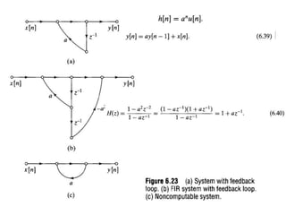


![• In some cases there is no way to order the computations so that the node
variables of a flow graph can be computed in sequence.
• Such a network is called noncomputable.
• A simple noncomputable network is shown in fig 6.23c.
• The difference equation for this network is
• In this form we cannot compute y[n] because the right hand side of the equation
involves the quantity we wish to compute.
• The fact that a flow graph is noncomputable deos not mean the equations
represented by the flow graph cannot be solved.
• Solution of this equation is
•](https://image.slidesharecdn.com/structuresfordiscrete-timesystems-220124032144/85/Structures-for-discrete-time-systems-33-320.jpg)


![Direct form
• Fir system, the system function has only zeros and since the coefficients ak are all
zero, the difference equation of eq.6.9 reduces to
• This can be recognized as the discrete convolution of x[n] with the impulse
response](https://image.slidesharecdn.com/structuresfordiscrete-timesystems-220124032144/85/Structures-for-discrete-time-systems-36-320.jpg)
![• Because of the chain of delay elements across the top of the diagram, this
structure is also referred to as a tapped delay line structure or a transversal filter
structure.
• From the figure 6.31, the signal at each tap along this chain is weighted by the
appropriate coefficient, and the resulting products are summed to form the output
y[n].
• The transposed direct form for the FIR case is obtained by applying the
transposition theorem to figure 6.31 or equivalently, by setting the coefficients ak
to zero in figure 6.32](https://image.slidesharecdn.com/structuresfordiscrete-timesystems-220124032144/85/Structures-for-discrete-time-systems-37-320.jpg)


![• Equations 6.50 to 6.53 imply structures with either
coefficient multipliers, rather than the M coefficient multipliers of the general
direct form structure of figure 6.31.
• Figure 6.34 shows the structure implied by eq 6.50 and figure 6.35 shows the
structure implied by eq 6.52.
• Symmetry conditions of equation 6.49a and 6.49b cause the zeros of H(z) to
occure in mirror-image pairs.
• That is, if z0 of H(z), then 1/z0 is also a zero of H(z).
• Further more, if h[n] is real, then the zeros of H(z) occur in complex-conjugate
pairs.](https://image.slidesharecdn.com/structuresfordiscrete-timesystems-220124032144/85/Structures-for-discrete-time-systems-43-320.jpg)


Structures for discrete time systems
- 1. Structures for Discrete-time systems
- 2. Introduction • A system difference equation, the impulse response, and the system function are equivalent characterizations of the input – output relation of a linear time invariant discrete-time system. • When such systems are implemented with discrete-time analog or digital hardware, the difference equation or the system function representation must be converted to an algorithm or structure that can be realized in the desired technology. • A system described by linear constant – coefficient difference equations can be represented by structures consisting of an interconnection of the basic operations of addition, multiplication by a constant, and delay, the exact implementation of which is dictated by the technology to be used.
- 3. • And the first order difference equation that is satisfied by the input and output sequences is • since the system has an infinite-duration impulse response, it is not possible to implement the system by discrete convolution. • However, rewriting the equation 3 in the form provides the basis for an algorithm for recursive computation of the output at any time n in terms of the previous output y[n-1], the current input sample x[n], and the previous input sample x[n-1]. • Recurrence formula for computing the output from past values of the output and present and past values of the input, the system will be linear and time invariant.
- 4. Block diagram representation of linear constant coefficient difference equation • The implementation of a linear time-invariant discrete time system by iteratively evaluating a recurrence formula obtained from a difference equation requires that delayed values of output and input, and intermediate sequences be available. • The delay of sequence values implies the need for storage of past sequence values. • We use multiplication of delayed sequence values by the coefficients, as well as adding the resulting products. • The basic elements required for the implementation of a linear time-invariant discrete-time system are adders, multipliers, and memory for storing delayed sequence values. • The interconnection of these basic elements is conveniently depicted by block diagrams composed of the basic pictorial symbols.
- 5. •
- 6. • Computational algorithm for implementing the system. • When the system is implemented on either a general purpose computer or a digital signal processing chip, network structures such as the show in figure serve as the basis for a program that implements the system. • The block diagram is the basis for determining a hardware architecture for the system. • For design a system we must provide storage for the delayed variables and also coefficients of the difference equation. • Figure 6.2 conveniently depicts the complexity of the associated computational algorithm, the steps of the algorithm, and the amount of hardware required to realize the system. • Example 6.1 can be generalized to higher order difference equations of the form
- 8. • The assumption of a two-input adder implies that the additions are done in a specified order. That is, figure 6.3 shows that the products • must be computed, then added, and the resulting sum added to and so on. • After y[n] has been computed , the delay variables must be updated by moving Y[n-N+1] into the register holding y[n-N], and so on.
- 10. • Specifically, the minimum number of delays required is, in general, max (N,M). • An implementation with minimum number of delay elements is commonly referred to as a canonic form implementation. • The non canonic block diagram in figure 6.3 is referred to as the direct form I implementation of the general Nth-order system because it is a direct realization of the difference equation satisfied by the input x[n] and the output y[n], which in turn can be written by directly form the system function by inspection. • From fig 6.5 is an appropriate realization structure for H (z) given by eq 6.8 , we can go directly back and forth in a straightforward manner between the system function and the block diagram.
- 11. Signal flow graph representation of linear constant-coefficient difference equations •A signal flow graph representation of a difference equation is essentially the same as a block diagram representation, except for a few notational differences. •Formally, a signal flow graph is a network of directed branches that connect at nodes. •Associated with each node is a variable or node value. •The value associated with node k might be denoted wk . •Branch (j,k) denotes a branch originating at node j and terminating at node k, with the direction from j to k being indicated by an arrowhead on the branch.
- 12. • By definition, the value at each node in a graph is the sum of the outputs of a the branches entering the node. • Source node: nodes that have no entering branches. • source nodes are used to represent the injection of external inputs or signal sources into a graph. • Sink node: nodes that have only entering branches. • sink nodes are used to extract outputs from a graph. • Source and Sink nodes and simple branch gains are illustrated in figure. • The linear equations represented by the figure are as follows: • Addition, multiplication by a constant, and delay are basic operations required to implement a linear constant- coefficient difference equation. • Since these are all linear operations, it is possible to use signal flow graph notation to depict algorithms for implementing linear time-invariant discrete time system.
- 13. • Example that signal flow graph concepts just discussed can be applied to the representation of a difference equation, consider the block diagram, which is the direct form II realization of the system whose system function given by eq 6.1
- 14. • The equations represented by figure 6.11 are • Difference between the two is that nodes in the flow graph represent both branching points and adders, whereas in the block diagram a special symbol is used for adders. • An adder in the block diagram is represented in the signal flow graph by a bode that has to incoming branches. • Signal flow graphs are therefore totally equivalent to block diagrams as pictorial representations of difference equations.
- 15. • Equations are define a multistep algorithm for computing the output of the linear time-invariant system from the input sequence x[n]. • Equations 6.18a to 6.18e cannot be computed in arbitrary order • Equations a to c require multiplications and additions, but equation b and e simply rename variables. • Equation d represents the updating of the memory of the system. • The flow graph represents a set of difference equations, with one equation being written at each node of the network. • In the case of the flow graph of figure 6.11 can be eliminate some of the variables rather easily to obtain the pair of equations. • Which are in the form of eq 6.15a and 6.15b i.e., in direct form II. • Often, the manipulation of the difference equations of a flow graph is difficult when dealing with time domain variables, due to feedback delay variables. • In such cases, it is always possible to work with z-transform representation, where in all branches are simple gains.
- 16. Basic structures for IIR systems
- 17. • For any given rational system function, a wide variety of equivalent sets of difference equations or network structures exists. • One consideration in the choice among these different structures is computational complexity. • In some digital implementation, structures with fewest constant multipliers are the fewest delay branches are often most desirable. • Multiplication is a time consuming and costly operation in digital hardware and because each delay element corresponds to a memory register. • Reduction in the number of constant multipliers means an increase in speed, and a reduction in the number of delay elements means a reduction in memory requirements.
- 18. • In VLSI implementations, in which the area of a chip is often an important measure of efficiency. • Modularity and simplicity of data transfer on the chip are also frequently very desirable in such implementations. • In multiprocessor implementations, the most important considerations are often related to partitioning of the algorithm and communication requirements between processors. • Major consideration is the effects of a finite register length and finite precision arithmetic.
- 19. • Block diagram representation of the direct form I and direct form II, structures for a linear time-invariant system whose input and output satisfy a difference equation of the form • With the corresponding rational system function • In figure 6.14 the direct form I structure of figure 6.3 is shown using signal flow graph conventions, and figure 6.15 shows the signal flow graph representation of the direct form II structure of figure 6.5. • Let us assume for convenience that N=M. Direct forms
- 20. •drawn the flow graph so that each node has no more than two inputs. •A node in a signal flow graph may have any number of inputs, but, as indicated earlier, this two input convention results in a graph that is more closely related to programs and architectures for implementing the computation of the difference equations represented by graph.
- 22. Cascade form • The direct form structures were obtained directly from the system function H(z), written as a ratio of polynomials in the variable z-1 as in equation 6.27 • I if we factor the numerator and denominator polynomials, we can express H(z), in the form • with the corresponding rational system function • where M=M1+2M2 and N=N1+2N2. • I
- 24. • In this expression, the first order factors represent real zeros at fk and real poles at ck , and the second-order factors represent complex conjugate pairs of zeros at gk and gk* and complex conjugate pairs of poles at dk and dk*. • When all the coefficients in equation 6.27 are real, then this represents the most general distribution of poles and zeros. • Eq 6.29 suggests a class of structures consisting of a cascade of first and second order systems. • It is often desirable to implement the cascade realization using a minimum of storage and computation. • Many types of implementations is obtained by combining pairs of real factors and complex conjugate pairs into second order factors so that eq 6.29 can be expressed as
- 25. • Where is the largest integer contained in . • writing in this form, we have assumed that and that the real poles and zeros have been combined in pairs. • if there are an odd number of real zeros/poles, one of the coefficients / will be zero. • Implement a cascade structure with a minimum number of multiplications and a minimum number of delay elements if we use the direct form II structure for each second-order section. • A cascade structure for a sixth-order system using three direct form II second order sections in shown in figure 6.18
- 26. • If there are second order sections, there are pairings of the poles with zeros and ordering of the resulting second order sections, or a total of different pairings and orderings. • Although these all have the same overall system function and corresponding input- output relation when infinite-precision arithmetic is used.
- 27. Parallel form • To factoring the numerator and denominator polynomials of H(z), we can express a rational system function as given by eq 6.27 or 6.29 as a partial fraction expansion in the form • In this form, the system function can be interpreted as representing a parallel combination of first and second-order IIR systems, with possibly simple scaled delay paths. • Alternatively, we may group the real poles in pairs, so that H(z) can be expressed as • is the largest integer contained in is negative, the first sum is not present. •
- 28. •A typical example for N=M=6 is shown in figure 6.20. •The general difference equations for the parallel form with second-order direct form II sections are
- 29. Feedback in IIR Systems • Feedback loops; i.e., they have closed paths that begin at a node and return to that node by traversing branches only in the direction of their arrowheads. • in the flow graph implies that a node variable in a loop depends directly or indirectly on itself. • This type of loops are necessarily to generate infinitely long impulse responses. • If a network with no feed back loops. • Any path from the input to the output can pass through each delay element only once. • Therefore, the longest delay between the input and output would occur for a path that passes through all of the delay elements in the network. • Thus, for a network with no loops, the impulse response is no longer than the total number of delay elements in the network. • If a network has no loops, then the system function has only zeros, and the number of zeros can be no more than the number of delay elements in the network.
- 31. • In figure 6.23a when the input is the impulse sequence, the single input sample continually re-circulates in the feedback loop with either increasing (if |a|>1) or decreasing ( if |a|<1) amplitude due to multiplication by the constant a, so that the impulse response is • This is the way that feedback can create an infinitely long impulse response. • If a system function has poles, a corresponding block diagram or signal flow graph will have feedback loops. • Neither poles in the system function nor loops in the network are sufficient for the impulse response to be infinitely long. • Figure 6.23b shows a network with a loop, but with an impulse response of finite length. • This is because the pole of the system function cancels with zero;
- 32. • i.e., for figure 6.3b • Impulse response of this system is • The system is a simple example of a general class of FIR systems called frequency-sampling systems. • Loops in a network pose special problems in implementing the computations implied by the network. • It must be possible to compute the node variables in a network in sequences such that all necessary values are available when needed.
- 33. • In some cases there is no way to order the computations so that the node variables of a flow graph can be computed in sequence. • Such a network is called noncomputable. • A simple noncomputable network is shown in fig 6.23c. • The difference equation for this network is • In this form we cannot compute y[n] because the right hand side of the equation involves the quantity we wish to compute. • The fact that a flow graph is noncomputable deos not mean the equations represented by the flow graph cannot be solved. • Solution of this equation is •
- 34. • Flow graph does not represent a set of difference equations that can be solved successively for the node variables. • The key to the computability of a flow graph is that all loops must contain at least one unit delay element. • Thus, in manipulating flow graphs representing implementations of linear time- invariant systems, we must be careful not to create delay free loops.
- 35. Basic network structures for FIR SYSTEMS
- 36. Direct form • Fir system, the system function has only zeros and since the coefficients ak are all zero, the difference equation of eq.6.9 reduces to • This can be recognized as the discrete convolution of x[n] with the impulse response
- 37. • Because of the chain of delay elements across the top of the diagram, this structure is also referred to as a tapped delay line structure or a transversal filter structure. • From the figure 6.31, the signal at each tap along this chain is weighted by the appropriate coefficient, and the resulting products are summed to form the output y[n]. • The transposed direct form for the FIR case is obtained by applying the transposition theorem to figure 6.31 or equivalently, by setting the coefficients ak to zero in figure 6.32
- 38. Cascade form • The cascade form for FIR systems is obtained by factoring the polynomial system function. • Represent H(z) as • Where is the largest integer contained in • If M is odd, one of the coefficients b2k will be zero, since H(z) in that case would have an odd number of real zeros. • The flow graph representing eq. 6.48 is shown in figure 6.33, which is identical in form to figure 6.18 with the coefficients a1k and a2k all zero.
- 39. Structures for linear-phase FIR systems • FIR systems have generalized linear phase if the impulse response satisfies the symmetry condition • With either these conditions, the number of coefficient multipliers can be essentially halved. • To see this, consider the following manipulations of the discrete convolution equation, assuming that M is an even integer corresponding to type I or type III systems:
- 43. • Equations 6.50 to 6.53 imply structures with either coefficient multipliers, rather than the M coefficient multipliers of the general direct form structure of figure 6.31. • Figure 6.34 shows the structure implied by eq 6.50 and figure 6.35 shows the structure implied by eq 6.52. • Symmetry conditions of equation 6.49a and 6.49b cause the zeros of H(z) to occure in mirror-image pairs. • That is, if z0 of H(z), then 1/z0 is also a zero of H(z). • Further more, if h[n] is real, then the zeros of H(z) occur in complex-conjugate pairs.
- 44. • If a zero is on the unit circle, its reciprocal is also its conjugate. • Complex zeros on the unit circle are conveniently grouped into pairs. • Zeros at z=+/- 1 are their own reciprocal and complex conjugate. • The four cases are summarized in figure 6.36, where the zeros at are considered as a group of four. • the zeros at z2 and 1/z2 are considered as a group of two, as are the zeros at z3 and z3*. • The zero at z4 is considered singly.
- 46. Number representations • Signal values and system coefficients represent in real number system. • In analog discrete time system, limited precision of the components of a circuit makes it difficult to realize coefficients exactly • In digital system signal representation we must use finite precision • Most general purpose digital computers DSP chips, or special purpose hardware uses binary number system. • Implementing arithmetic one of the bits of the binary number is assumed to indicate the algebraic sign of number. • Formats such as sign and magnitude, one’s and two’s complement. ‘
- 47. • A real number can be represented with infinite precision in two’s-complement form as • Xm is an arbitrary scale factor • bi ‘s are either 0 or 1. • bo is referred to as sign bit. If b=0; then • I if b=1; then • Any real number whose magnitude is less than or equal to Xm can be represented by this 6.55 equation. • So that arbitrary real number x would require an infinite number of bits for its exact binary representation.
- 48. • If we use only its exact binary representation, if we use only finite number of bits (B+1), then the representaion of equation 6.55 • The resulting binary representation is quantized, so that the samllest difference between numbers is • In this case quantized numbers are in the range • The fractional part of can be represented with the positional notation
- 50. • The operation of quantizing a number to (B+1) bits can be implemented by rounding or by truncation, but in either case quantization is a nonlinear memory less operation. • Input –output relation for two’s complement rounding and truncation, respectively, for the case B=2. • Considering the effects of quantization, we often define the quantization error as • For the case of two’s complement rounding • for two’s complement truncation
- 51. •If a number is larger than Xm must implement some method of determining the quantized result. in the two’s complement arithmetic system, this need arises when we add two numbers sum is greater than Xm •For ex 4 bit two’s complement number 0111, which in decimal form is 7. •If we add the number 0001, the carry propagates all the way to the sign bit, so that the result is 1000, which in decimal is 8. •Thus the resulting error can be very large when over flow occurs. •Figure 6.38a shows two’s complement quantizer, including the effect of regular two’s complement arithmetic overflow. •Alternative is called saturation overflo w or clipping .
- 52. • Both quantization and overflow introduce errors in digital representations of numbers. • In digital signal processing implementation, it is common to assume that all signal variables and all coefficients are binary fractions. • If we multiply a (B+1) bit signal variable by a (B+1) bits coefficient, the result is a (2B+1) bit fraction that can be conveniently reduced to (B+1) bits by rounding or truncating the least significant bits. • For example, in fixed point computations, it is common to assume that each binary number has a scale factor of the form . • C=2 implies that the binary point is actually located between b2 and b3 of the binary word in equation 6.58 • Another away about scale factor Xm leads to the floating point representations • Characteristic and mantissa are each represented explicitly as binary numbers in floating point arithmetic system. • Floating point representations provide a convenient means for maintaining both a wide dynamic range and a small quantization noise;
Editor's Notes
- #8: Recurrence formula for y[n] in terms of a linear combination of past values of the output sequence and current and past values of the input sequence leads to the relation