Subgradient Methods for Huge-Scale Optimization Problems - Юрий Нестеров, Catholic University of Louvain, Belgium
1 like637 views

The document discusses subgradient methods for huge-scale optimization problems, highlighting the challenges and complexities involved in sparse optimization. It emphasizes the importance of sparsity in accelerating computations and provides examples of computational expenses for various algorithms. The author outlines strategies for sparse updates which significantly reduce the computational burden in comparison to traditional methods.


![When it can work?
Simple methods: No full-vector operations! (Is it possible?)
Simple problems: Functions with sparse gradients.
Let us try:
1 Quadratic function f (x) = 1
2 Ax, x − b, x . The gradient
f (x) = Ax − b, x ∈ RN
,
is not sparse even if A is sparse.
2 Piece-wise linear function g(x) = max
1≤i≤m
[ ai , x − b(i)].
Yu. Nesterov Subgradient methods for huge-scale problems 7/22](https://image.slidesharecdn.com/sublinbm1-141114054915-conversion-gate02/85/Subgradient-Methods-for-Huge-Scale-Optimization-Problems-Catholic-University-of-Louvain-Belgium-59-320.jpg)
![When it can work?
Simple methods: No full-vector operations! (Is it possible?)
Simple problems: Functions with sparse gradients.
Let us try:
1 Quadratic function f (x) = 1
2 Ax, x − b, x . The gradient
f (x) = Ax − b, x ∈ RN
,
is not sparse even if A is sparse.
2 Piece-wise linear function g(x) = max
1≤i≤m
[ ai , x − b(i)]. Its
subgradient f (x) = ai(x), i(x) : f (x) = ai(x), x − b(i(x)),
Yu. Nesterov Subgradient methods for huge-scale problems 7/22](https://image.slidesharecdn.com/sublinbm1-141114054915-conversion-gate02/85/Subgradient-Methods-for-Huge-Scale-Optimization-Problems-Catholic-University-of-Louvain-Belgium-60-320.jpg)
![When it can work?
Simple methods: No full-vector operations! (Is it possible?)
Simple problems: Functions with sparse gradients.
Let us try:
1 Quadratic function f (x) = 1
2 Ax, x − b, x . The gradient
f (x) = Ax − b, x ∈ RN
,
is not sparse even if A is sparse.
2 Piece-wise linear function g(x) = max
1≤i≤m
[ ai , x − b(i)]. Its
subgradient f (x) = ai(x), i(x) : f (x) = ai(x), x − b(i(x)),
can be sparse is ai is sparse!
Yu. Nesterov Subgradient methods for huge-scale problems 7/22](https://image.slidesharecdn.com/sublinbm1-141114054915-conversion-gate02/85/Subgradient-Methods-for-Huge-Scale-Optimization-Problems-Catholic-University-of-Louvain-Belgium-61-320.jpg)
![When it can work?
Simple methods: No full-vector operations! (Is it possible?)
Simple problems: Functions with sparse gradients.
Let us try:
1 Quadratic function f (x) = 1
2 Ax, x − b, x . The gradient
f (x) = Ax − b, x ∈ RN
,
is not sparse even if A is sparse.
2 Piece-wise linear function g(x) = max
1≤i≤m
[ ai , x − b(i)]. Its
subgradient f (x) = ai(x), i(x) : f (x) = ai(x), x − b(i(x)),
can be sparse is ai is sparse!
But:
Yu. Nesterov Subgradient methods for huge-scale problems 7/22](https://image.slidesharecdn.com/sublinbm1-141114054915-conversion-gate02/85/Subgradient-Methods-for-Huge-Scale-Optimization-Problems-Catholic-University-of-Louvain-Belgium-62-320.jpg)
![When it can work?
Simple methods: No full-vector operations! (Is it possible?)
Simple problems: Functions with sparse gradients.
Let us try:
1 Quadratic function f (x) = 1
2 Ax, x − b, x . The gradient
f (x) = Ax − b, x ∈ RN
,
is not sparse even if A is sparse.
2 Piece-wise linear function g(x) = max
1≤i≤m
[ ai , x − b(i)]. Its
subgradient f (x) = ai(x), i(x) : f (x) = ai(x), x − b(i(x)),
can be sparse is ai is sparse!
But: We need a fast procedure for updating max-type operations.
Yu. Nesterov Subgradient methods for huge-scale problems 7/22](https://image.slidesharecdn.com/sublinbm1-141114054915-conversion-gate02/85/Subgradient-Methods-for-Huge-Scale-Optimization-Problems-Catholic-University-of-Louvain-Belgium-63-320.jpg)


![Main advantages
Important examples (symmetric functions)
f (x) = x p, p ≥ 1, ψi,j (t1, t2) ≡ [ |t1|p + |t2|p ]1/p
,
Yu. Nesterov Subgradient methods for huge-scale problems 9/22](https://image.slidesharecdn.com/sublinbm1-141114054915-conversion-gate02/85/Subgradient-Methods-for-Huge-Scale-Optimization-Problems-Catholic-University-of-Louvain-Belgium-71-320.jpg)
![Main advantages
Important examples (symmetric functions)
f (x) = x p, p ≥ 1, ψi,j (t1, t2) ≡ [ |t1|p + |t2|p ]1/p
,
f (x) = ln
n
i=1
ex(i)
, ψi,j (t1, t2) ≡ ln (et1 + et2 ) ,
Yu. Nesterov Subgradient methods for huge-scale problems 9/22](https://image.slidesharecdn.com/sublinbm1-141114054915-conversion-gate02/85/Subgradient-Methods-for-Huge-Scale-Optimization-Problems-Catholic-University-of-Louvain-Belgium-72-320.jpg)
![Main advantages
Important examples (symmetric functions)
f (x) = x p, p ≥ 1, ψi,j (t1, t2) ≡ [ |t1|p + |t2|p ]1/p
,
f (x) = ln
n
i=1
ex(i)
, ψi,j (t1, t2) ≡ ln (et1 + et2 ) ,
f (x) = max
1≤i≤n
x(i), ψi,j (t1, t2) ≡ max {t1, t2} .
Yu. Nesterov Subgradient methods for huge-scale problems 9/22](https://image.slidesharecdn.com/sublinbm1-141114054915-conversion-gate02/85/Subgradient-Methods-for-Huge-Scale-Optimization-Problems-Catholic-University-of-Louvain-Belgium-73-320.jpg)
![Main advantages
Important examples (symmetric functions)
f (x) = x p, p ≥ 1, ψi,j (t1, t2) ≡ [ |t1|p + |t2|p ]1/p
,
f (x) = ln
n
i=1
ex(i)
, ψi,j (t1, t2) ≡ ln (et1 + et2 ) ,
f (x) = max
1≤i≤n
x(i), ψi,j (t1, t2) ≡ max {t1, t2} .
The binary tree requires only n − 1 auxiliary cells.
Yu. Nesterov Subgradient methods for huge-scale problems 9/22](https://image.slidesharecdn.com/sublinbm1-141114054915-conversion-gate02/85/Subgradient-Methods-for-Huge-Scale-Optimization-Problems-Catholic-University-of-Louvain-Belgium-74-320.jpg)
![Main advantages
Important examples (symmetric functions)
f (x) = x p, p ≥ 1, ψi,j (t1, t2) ≡ [ |t1|p + |t2|p ]1/p
,
f (x) = ln
n
i=1
ex(i)
, ψi,j (t1, t2) ≡ ln (et1 + et2 ) ,
f (x) = max
1≤i≤n
x(i), ψi,j (t1, t2) ≡ max {t1, t2} .
The binary tree requires only n − 1 auxiliary cells.
Its value needs n − 1 applications of ψi,j (·, ·) ( ≡ operations).
Yu. Nesterov Subgradient methods for huge-scale problems 9/22](https://image.slidesharecdn.com/sublinbm1-141114054915-conversion-gate02/85/Subgradient-Methods-for-Huge-Scale-Optimization-Problems-Catholic-University-of-Louvain-Belgium-75-320.jpg)
![Main advantages
Important examples (symmetric functions)
f (x) = x p, p ≥ 1, ψi,j (t1, t2) ≡ [ |t1|p + |t2|p ]1/p
,
f (x) = ln
n
i=1
ex(i)
, ψi,j (t1, t2) ≡ ln (et1 + et2 ) ,
f (x) = max
1≤i≤n
x(i), ψi,j (t1, t2) ≡ max {t1, t2} .
The binary tree requires only n − 1 auxiliary cells.
Its value needs n − 1 applications of ψi,j (·, ·) ( ≡ operations).
If x+ differs from x in one entry only, then for re-computing
f (x+) we need only k ≡ log2 n operations.
Yu. Nesterov Subgradient methods for huge-scale problems 9/22](https://image.slidesharecdn.com/sublinbm1-141114054915-conversion-gate02/85/Subgradient-Methods-for-Huge-Scale-Optimization-Problems-Catholic-University-of-Louvain-Belgium-76-320.jpg)
![Main advantages
Important examples (symmetric functions)
f (x) = x p, p ≥ 1, ψi,j (t1, t2) ≡ [ |t1|p + |t2|p ]1/p
,
f (x) = ln
n
i=1
ex(i)
, ψi,j (t1, t2) ≡ ln (et1 + et2 ) ,
f (x) = max
1≤i≤n
x(i), ψi,j (t1, t2) ≡ max {t1, t2} .
The binary tree requires only n − 1 auxiliary cells.
Its value needs n − 1 applications of ψi,j (·, ·) ( ≡ operations).
If x+ differs from x in one entry only, then for re-computing
f (x+) we need only k ≡ log2 n operations.
Thus, we can have pure subgradient minimization schemes with
Yu. Nesterov Subgradient methods for huge-scale problems 9/22](https://image.slidesharecdn.com/sublinbm1-141114054915-conversion-gate02/85/Subgradient-Methods-for-Huge-Scale-Optimization-Problems-Catholic-University-of-Louvain-Belgium-77-320.jpg)
![Main advantages
Important examples (symmetric functions)
f (x) = x p, p ≥ 1, ψi,j (t1, t2) ≡ [ |t1|p + |t2|p ]1/p
,
f (x) = ln
n
i=1
ex(i)
, ψi,j (t1, t2) ≡ ln (et1 + et2 ) ,
f (x) = max
1≤i≤n
x(i), ψi,j (t1, t2) ≡ max {t1, t2} .
The binary tree requires only n − 1 auxiliary cells.
Its value needs n − 1 applications of ψi,j (·, ·) ( ≡ operations).
If x+ differs from x in one entry only, then for re-computing
f (x+) we need only k ≡ log2 n operations.
Thus, we can have pure subgradient minimization schemes with
Sublinear Iteration Cost
.
Yu. Nesterov Subgradient methods for huge-scale problems 9/22](https://image.slidesharecdn.com/sublinbm1-141114054915-conversion-gate02/85/Subgradient-Methods-for-Huge-Scale-Optimization-Problems-Catholic-University-of-Louvain-Belgium-78-320.jpg)


![Mathematical formulation: quadratic problem
Let E ∈ RN×N be an incidence matrix of the connections graph.
Denote e = (1, . . . , 1)T ∈ RN and ¯E = E · diag (ET e)−1.
Since, ¯ET e = e, this matrix is stochastic.
Problem: Find x∗ ≥ 0 : ¯Ex∗ = x∗, x∗ = 0.
The size is very big!
Known technique:
Regularization + Fixed Point (Google Founders, B.Polyak &
coauthors, etc.)
N09: Solve it by random CD-method as applied to
1
2
¯Ex − x 2 + γ
2 [ e, x − 1]2, γ > 0.
Yu. Nesterov Subgradient methods for huge-scale problems 16/22](https://image.slidesharecdn.com/sublinbm1-141114054915-conversion-gate02/85/Subgradient-Methods-for-Huge-Scale-Optimization-Problems-Catholic-University-of-Louvain-Belgium-151-320.jpg)
![Mathematical formulation: quadratic problem
Let E ∈ RN×N be an incidence matrix of the connections graph.
Denote e = (1, . . . , 1)T ∈ RN and ¯E = E · diag (ET e)−1.
Since, ¯ET e = e, this matrix is stochastic.
Problem: Find x∗ ≥ 0 : ¯Ex∗ = x∗, x∗ = 0.
The size is very big!
Known technique:
Regularization + Fixed Point (Google Founders, B.Polyak &
coauthors, etc.)
N09: Solve it by random CD-method as applied to
1
2
¯Ex − x 2 + γ
2 [ e, x − 1]2, γ > 0.
Main drawback: No interpretation for the objective function!
Yu. Nesterov Subgradient methods for huge-scale problems 16/22](https://image.slidesharecdn.com/sublinbm1-141114054915-conversion-gate02/85/Subgradient-Methods-for-Huge-Scale-Optimization-Problems-Catholic-University-of-Louvain-Belgium-152-320.jpg)


![Nonsmooth formulation of Google Problem
Main property of spectral radius (A ≥ 0)
If A ∈ Rn×n
+ , then ρ(A) = min
x≥0
max
1≤i≤n
1
x(i) ei , Ax .
The minimum is attained at the corresponding eigenvector.
Since ρ(¯E) = 1, our problem is as follows:
f (x)
def
= max
1≤i≤N
[ ei , ¯Ex − x(i)] → min
x≥0
.
Yu. Nesterov Subgradient methods for huge-scale problems 17/22](https://image.slidesharecdn.com/sublinbm1-141114054915-conversion-gate02/85/Subgradient-Methods-for-Huge-Scale-Optimization-Problems-Catholic-University-of-Louvain-Belgium-156-320.jpg)
![Nonsmooth formulation of Google Problem
Main property of spectral radius (A ≥ 0)
If A ∈ Rn×n
+ , then ρ(A) = min
x≥0
max
1≤i≤n
1
x(i) ei , Ax .
The minimum is attained at the corresponding eigenvector.
Since ρ(¯E) = 1, our problem is as follows:
f (x)
def
= max
1≤i≤N
[ ei , ¯Ex − x(i)] → min
x≥0
.
Interpretation: Increase self-confidence!
Yu. Nesterov Subgradient methods for huge-scale problems 17/22](https://image.slidesharecdn.com/sublinbm1-141114054915-conversion-gate02/85/Subgradient-Methods-for-Huge-Scale-Optimization-Problems-Catholic-University-of-Louvain-Belgium-157-320.jpg)
![Nonsmooth formulation of Google Problem
Main property of spectral radius (A ≥ 0)
If A ∈ Rn×n
+ , then ρ(A) = min
x≥0
max
1≤i≤n
1
x(i) ei , Ax .
The minimum is attained at the corresponding eigenvector.
Since ρ(¯E) = 1, our problem is as follows:
f (x)
def
= max
1≤i≤N
[ ei , ¯Ex − x(i)] → min
x≥0
.
Interpretation: Increase self-confidence!
Since f ∗ = 0, we can apply Polyak’s method with sparse updates.
Yu. Nesterov Subgradient methods for huge-scale problems 17/22](https://image.slidesharecdn.com/sublinbm1-141114054915-conversion-gate02/85/Subgradient-Methods-for-Huge-Scale-Optimization-Problems-Catholic-University-of-Louvain-Belgium-158-320.jpg)
![Nonsmooth formulation of Google Problem
Main property of spectral radius (A ≥ 0)
If A ∈ Rn×n
+ , then ρ(A) = min
x≥0
max
1≤i≤n
1
x(i) ei , Ax .
The minimum is attained at the corresponding eigenvector.
Since ρ(¯E) = 1, our problem is as follows:
f (x)
def
= max
1≤i≤N
[ ei , ¯Ex − x(i)] → min
x≥0
.
Interpretation: Increase self-confidence!
Since f ∗ = 0, we can apply Polyak’s method with sparse updates.
Additional features; the optimal set X∗ is a convex cone.
Yu. Nesterov Subgradient methods for huge-scale problems 17/22](https://image.slidesharecdn.com/sublinbm1-141114054915-conversion-gate02/85/Subgradient-Methods-for-Huge-Scale-Optimization-Problems-Catholic-University-of-Louvain-Belgium-159-320.jpg)
![Nonsmooth formulation of Google Problem
Main property of spectral radius (A ≥ 0)
If A ∈ Rn×n
+ , then ρ(A) = min
x≥0
max
1≤i≤n
1
x(i) ei , Ax .
The minimum is attained at the corresponding eigenvector.
Since ρ(¯E) = 1, our problem is as follows:
f (x)
def
= max
1≤i≤N
[ ei , ¯Ex − x(i)] → min
x≥0
.
Interpretation: Increase self-confidence!
Since f ∗ = 0, we can apply Polyak’s method with sparse updates.
Additional features; the optimal set X∗ is a convex cone.
If x0 = e, then the whole sequence is separated from zero:
Yu. Nesterov Subgradient methods for huge-scale problems 17/22](https://image.slidesharecdn.com/sublinbm1-141114054915-conversion-gate02/85/Subgradient-Methods-for-Huge-Scale-Optimization-Problems-Catholic-University-of-Louvain-Belgium-160-320.jpg)
![Nonsmooth formulation of Google Problem
Main property of spectral radius (A ≥ 0)
If A ∈ Rn×n
+ , then ρ(A) = min
x≥0
max
1≤i≤n
1
x(i) ei , Ax .
The minimum is attained at the corresponding eigenvector.
Since ρ(¯E) = 1, our problem is as follows:
f (x)
def
= max
1≤i≤N
[ ei , ¯Ex − x(i)] → min
x≥0
.
Interpretation: Increase self-confidence!
Since f ∗ = 0, we can apply Polyak’s method with sparse updates.
Additional features; the optimal set X∗ is a convex cone.
If x0 = e, then the whole sequence is separated from zero:
x∗, e
Yu. Nesterov Subgradient methods for huge-scale problems 17/22](https://image.slidesharecdn.com/sublinbm1-141114054915-conversion-gate02/85/Subgradient-Methods-for-Huge-Scale-Optimization-Problems-Catholic-University-of-Louvain-Belgium-161-320.jpg)
![Nonsmooth formulation of Google Problem
Main property of spectral radius (A ≥ 0)
If A ∈ Rn×n
+ , then ρ(A) = min
x≥0
max
1≤i≤n
1
x(i) ei , Ax .
The minimum is attained at the corresponding eigenvector.
Since ρ(¯E) = 1, our problem is as follows:
f (x)
def
= max
1≤i≤N
[ ei , ¯Ex − x(i)] → min
x≥0
.
Interpretation: Increase self-confidence!
Since f ∗ = 0, we can apply Polyak’s method with sparse updates.
Additional features; the optimal set X∗ is a convex cone.
If x0 = e, then the whole sequence is separated from zero:
x∗, e ≤ x∗, xk
Yu. Nesterov Subgradient methods for huge-scale problems 17/22](https://image.slidesharecdn.com/sublinbm1-141114054915-conversion-gate02/85/Subgradient-Methods-for-Huge-Scale-Optimization-Problems-Catholic-University-of-Louvain-Belgium-162-320.jpg)
![Nonsmooth formulation of Google Problem
Main property of spectral radius (A ≥ 0)
If A ∈ Rn×n
+ , then ρ(A) = min
x≥0
max
1≤i≤n
1
x(i) ei , Ax .
The minimum is attained at the corresponding eigenvector.
Since ρ(¯E) = 1, our problem is as follows:
f (x)
def
= max
1≤i≤N
[ ei , ¯Ex − x(i)] → min
x≥0
.
Interpretation: Increase self-confidence!
Since f ∗ = 0, we can apply Polyak’s method with sparse updates.
Additional features; the optimal set X∗ is a convex cone.
If x0 = e, then the whole sequence is separated from zero:
x∗, e ≤ x∗, xk ≤ x∗
1 · xk ∞
Yu. Nesterov Subgradient methods for huge-scale problems 17/22](https://image.slidesharecdn.com/sublinbm1-141114054915-conversion-gate02/85/Subgradient-Methods-for-Huge-Scale-Optimization-Problems-Catholic-University-of-Louvain-Belgium-163-320.jpg)
![Nonsmooth formulation of Google Problem
Main property of spectral radius (A ≥ 0)
If A ∈ Rn×n
+ , then ρ(A) = min
x≥0
max
1≤i≤n
1
x(i) ei , Ax .
The minimum is attained at the corresponding eigenvector.
Since ρ(¯E) = 1, our problem is as follows:
f (x)
def
= max
1≤i≤N
[ ei , ¯Ex − x(i)] → min
x≥0
.
Interpretation: Increase self-confidence!
Since f ∗ = 0, we can apply Polyak’s method with sparse updates.
Additional features; the optimal set X∗ is a convex cone.
If x0 = e, then the whole sequence is separated from zero:
x∗, e ≤ x∗, xk ≤ x∗
1 · xk ∞ = x∗, e · xk ∞.
Yu. Nesterov Subgradient methods for huge-scale problems 17/22](https://image.slidesharecdn.com/sublinbm1-141114054915-conversion-gate02/85/Subgradient-Methods-for-Huge-Scale-Optimization-Problems-Catholic-University-of-Louvain-Belgium-164-320.jpg)
![Nonsmooth formulation of Google Problem
Main property of spectral radius (A ≥ 0)
If A ∈ Rn×n
+ , then ρ(A) = min
x≥0
max
1≤i≤n
1
x(i) ei , Ax .
The minimum is attained at the corresponding eigenvector.
Since ρ(¯E) = 1, our problem is as follows:
f (x)
def
= max
1≤i≤N
[ ei , ¯Ex − x(i)] → min
x≥0
.
Interpretation: Increase self-confidence!
Since f ∗ = 0, we can apply Polyak’s method with sparse updates.
Additional features; the optimal set X∗ is a convex cone.
If x0 = e, then the whole sequence is separated from zero:
x∗, e ≤ x∗, xk ≤ x∗
1 · xk ∞ = x∗, e · xk ∞.
Goal: Find ¯x ≥ 0 such that ¯x ∞ ≥ 1 and f (¯x) ≤ .
Yu. Nesterov Subgradient methods for huge-scale problems 17/22](https://image.slidesharecdn.com/sublinbm1-141114054915-conversion-gate02/85/Subgradient-Methods-for-Huge-Scale-Optimization-Problems-Catholic-University-of-Louvain-Belgium-165-320.jpg)
![Nonsmooth formulation of Google Problem
Main property of spectral radius (A ≥ 0)
If A ∈ Rn×n
+ , then ρ(A) = min
x≥0
max
1≤i≤n
1
x(i) ei , Ax .
The minimum is attained at the corresponding eigenvector.
Since ρ(¯E) = 1, our problem is as follows:
f (x)
def
= max
1≤i≤N
[ ei , ¯Ex − x(i)] → min
x≥0
.
Interpretation: Increase self-confidence!
Since f ∗ = 0, we can apply Polyak’s method with sparse updates.
Additional features; the optimal set X∗ is a convex cone.
If x0 = e, then the whole sequence is separated from zero:
x∗, e ≤ x∗, xk ≤ x∗
1 · xk ∞ = x∗, e · xk ∞.
Goal: Find ¯x ≥ 0 such that ¯x ∞ ≥ 1 and f (¯x) ≤ .
(First condition is satisfied automatically.)
Yu. Nesterov Subgradient methods for huge-scale problems 17/22](https://image.slidesharecdn.com/sublinbm1-141114054915-conversion-gate02/85/Subgradient-Methods-for-Huge-Scale-Optimization-Problems-Catholic-University-of-Louvain-Belgium-166-320.jpg)


Subgradient Methods for Huge-Scale Optimization Problems - Юрий Нестеров, Catholic University of Louvain, Belgium
- 1. Subgradient methods for huge-scale optimization problems Yurii Nesterov, CORE/INMA (UCL) November 10, 2014 (Yandex, Moscow) Yu. Nesterov Subgradient methods for huge-scale problems 1/22
- 2. Outline 1 Problems sizes 2 Sparse Optimization problems 3 Sparse updates for linear operators 4 Fast updates in computational trees 5 Simple subgradient methods 6 Application examples 7 Computational experiments: Google problem Yu. Nesterov Subgradient methods for huge-scale problems 2/22
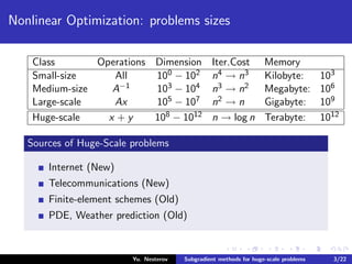
- 3. Nonlinear Optimization: problems sizes Class Operations Dimension Iter.Cost Memory Small-size All 100 − 102 n4 → n3 Kilobyte: 103 Medium-size A−1 103 − 104 n3 → n2 Megabyte: 106 Yu. Nesterov Subgradient methods for huge-scale problems 3/22
- 4. Nonlinear Optimization: problems sizes Class Operations Dimension Iter.Cost Memory Small-size All 100 − 102 n4 → n3 Kilobyte: 103 Medium-size A−1 103 − 104 n3 → n2 Megabyte: 106 Large-scale Ax 105 − 107 n2 → n Gigabyte: 109 Yu. Nesterov Subgradient methods for huge-scale problems 3/22
- 5. Nonlinear Optimization: problems sizes Class Operations Dimension Iter.Cost Memory Small-size All 100 − 102 n4 → n3 Kilobyte: 103 Medium-size A−1 103 − 104 n3 → n2 Megabyte: 106 Large-scale Ax 105 − 107 n2 → n Gigabyte: 109 Huge-scale x + y 108 − 1012 n → log n Terabyte: 1012 Yu. Nesterov Subgradient methods for huge-scale problems 3/22
- 6. Nonlinear Optimization: problems sizes Class Operations Dimension Iter.Cost Memory Small-size All 100 − 102 n4 → n3 Kilobyte: 103 Medium-size A−1 103 − 104 n3 → n2 Megabyte: 106 Large-scale Ax 105 − 107 n2 → n Gigabyte: 109 Huge-scale x + y 108 − 1012 n → log n Terabyte: 1012 Sources of Huge-Scale problems Yu. Nesterov Subgradient methods for huge-scale problems 3/22
- 7. Nonlinear Optimization: problems sizes Class Operations Dimension Iter.Cost Memory Small-size All 100 − 102 n4 → n3 Kilobyte: 103 Medium-size A−1 103 − 104 n3 → n2 Megabyte: 106 Large-scale Ax 105 − 107 n2 → n Gigabyte: 109 Huge-scale x + y 108 − 1012 n → log n Terabyte: 1012 Sources of Huge-Scale problems Internet (New) Telecommunications (New) Yu. Nesterov Subgradient methods for huge-scale problems 3/22
- 8. Nonlinear Optimization: problems sizes Class Operations Dimension Iter.Cost Memory Small-size All 100 − 102 n4 → n3 Kilobyte: 103 Medium-size A−1 103 − 104 n3 → n2 Megabyte: 106 Large-scale Ax 105 − 107 n2 → n Gigabyte: 109 Huge-scale x + y 108 − 1012 n → log n Terabyte: 1012 Sources of Huge-Scale problems Internet (New) Telecommunications (New) Finite-element schemes (Old) PDE, Weather prediction (Old) Yu. Nesterov Subgradient methods for huge-scale problems 3/22
- 9. Nonlinear Optimization: problems sizes Class Operations Dimension Iter.Cost Memory Small-size All 100 − 102 n4 → n3 Kilobyte: 103 Medium-size A−1 103 − 104 n3 → n2 Megabyte: 106 Large-scale Ax 105 − 107 n2 → n Gigabyte: 109 Huge-scale x + y 108 − 1012 n → log n Terabyte: 1012 Sources of Huge-Scale problems Internet (New) Telecommunications (New) Finite-element schemes (Old) PDE, Weather prediction (Old) Main hope: Sparsity. Yu. Nesterov Subgradient methods for huge-scale problems 3/22
- 10. Sparse problems Yu. Nesterov Subgradient methods for huge-scale problems 4/22
- 11. Sparse problems Problem: min x∈Q f (x), where Q is closed and convex in RN, Yu. Nesterov Subgradient methods for huge-scale problems 4/22
- 12. Sparse problems Problem: min x∈Q f (x), where Q is closed and convex in RN, and f (x) = Ψ(Ax), where Ψ is a simple convex function: Ψ(y1) ≥ Ψ(y2) + Ψ (y2), y1 − y2 , y1, y2 ∈ RM , Yu. Nesterov Subgradient methods for huge-scale problems 4/22
- 13. Sparse problems Problem: min x∈Q f (x), where Q is closed and convex in RN, and f (x) = Ψ(Ax), where Ψ is a simple convex function: Ψ(y1) ≥ Ψ(y2) + Ψ (y2), y1 − y2 , y1, y2 ∈ RM , A : RN → RM is a sparse matrix. Yu. Nesterov Subgradient methods for huge-scale problems 4/22
- 14. Sparse problems Problem: min x∈Q f (x), where Q is closed and convex in RN, and f (x) = Ψ(Ax), where Ψ is a simple convex function: Ψ(y1) ≥ Ψ(y2) + Ψ (y2), y1 − y2 , y1, y2 ∈ RM , A : RN → RM is a sparse matrix. Let p(x) def = # of nonzeros in x. Yu. Nesterov Subgradient methods for huge-scale problems 4/22
- 15. Sparse problems Problem: min x∈Q f (x), where Q is closed and convex in RN, and f (x) = Ψ(Ax), where Ψ is a simple convex function: Ψ(y1) ≥ Ψ(y2) + Ψ (y2), y1 − y2 , y1, y2 ∈ RM , A : RN → RM is a sparse matrix. Let p(x) def = # of nonzeros in x. Sparsity coefficient: γ(A) def = p(A) MN . Yu. Nesterov Subgradient methods for huge-scale problems 4/22
- 16. Sparse problems Problem: min x∈Q f (x), where Q is closed and convex in RN, and f (x) = Ψ(Ax), where Ψ is a simple convex function: Ψ(y1) ≥ Ψ(y2) + Ψ (y2), y1 − y2 , y1, y2 ∈ RM , A : RN → RM is a sparse matrix. Let p(x) def = # of nonzeros in x. Sparsity coefficient: γ(A) def = p(A) MN . Example 1: Matrix-vector multiplication Yu. Nesterov Subgradient methods for huge-scale problems 4/22
- 17. Sparse problems Problem: min x∈Q f (x), where Q is closed and convex in RN, and f (x) = Ψ(Ax), where Ψ is a simple convex function: Ψ(y1) ≥ Ψ(y2) + Ψ (y2), y1 − y2 , y1, y2 ∈ RM , A : RN → RM is a sparse matrix. Let p(x) def = # of nonzeros in x. Sparsity coefficient: γ(A) def = p(A) MN . Example 1: Matrix-vector multiplication Computation of vector Ax needs p(A) operations. Yu. Nesterov Subgradient methods for huge-scale problems 4/22
- 18. Sparse problems Problem: min x∈Q f (x), where Q is closed and convex in RN, and f (x) = Ψ(Ax), where Ψ is a simple convex function: Ψ(y1) ≥ Ψ(y2) + Ψ (y2), y1 − y2 , y1, y2 ∈ RM , A : RN → RM is a sparse matrix. Let p(x) def = # of nonzeros in x. Sparsity coefficient: γ(A) def = p(A) MN . Example 1: Matrix-vector multiplication Computation of vector Ax needs p(A) operations. Initial complexity MN is reduced in γ(A) times. Yu. Nesterov Subgradient methods for huge-scale problems 4/22
- 19. Example: Gradient Method Yu. Nesterov Subgradient methods for huge-scale problems 5/22
- 20. Example: Gradient Method x0 ∈ Q, xk+1 = πQ(xk − hf (xk)), k ≥ 0. Yu. Nesterov Subgradient methods for huge-scale problems 5/22
- 21. Example: Gradient Method x0 ∈ Q, xk+1 = πQ(xk − hf (xk)), k ≥ 0. Main computational expenses Yu. Nesterov Subgradient methods for huge-scale problems 5/22
- 22. Example: Gradient Method x0 ∈ Q, xk+1 = πQ(xk − hf (xk)), k ≥ 0. Main computational expenses Projection of simple set Q needs O(N) operations. Yu. Nesterov Subgradient methods for huge-scale problems 5/22
- 23. Example: Gradient Method x0 ∈ Q, xk+1 = πQ(xk − hf (xk)), k ≥ 0. Main computational expenses Projection of simple set Q needs O(N) operations. Displacement xk → xk − hf (xk) needs O(N) operations. Yu. Nesterov Subgradient methods for huge-scale problems 5/22
- 24. Example: Gradient Method x0 ∈ Q, xk+1 = πQ(xk − hf (xk)), k ≥ 0. Main computational expenses Projection of simple set Q needs O(N) operations. Displacement xk → xk − hf (xk) needs O(N) operations. f (x) = AT Ψ (Ax). Yu. Nesterov Subgradient methods for huge-scale problems 5/22
- 25. Example: Gradient Method x0 ∈ Q, xk+1 = πQ(xk − hf (xk)), k ≥ 0. Main computational expenses Projection of simple set Q needs O(N) operations. Displacement xk → xk − hf (xk) needs O(N) operations. f (x) = AT Ψ (Ax). If Ψ is simple, then the main efforts are spent for two matrix-vector multiplications: 2p(A). Yu. Nesterov Subgradient methods for huge-scale problems 5/22
- 26. Example: Gradient Method x0 ∈ Q, xk+1 = πQ(xk − hf (xk)), k ≥ 0. Main computational expenses Projection of simple set Q needs O(N) operations. Displacement xk → xk − hf (xk) needs O(N) operations. f (x) = AT Ψ (Ax). If Ψ is simple, then the main efforts are spent for two matrix-vector multiplications: 2p(A). Conclusion: Yu. Nesterov Subgradient methods for huge-scale problems 5/22
- 27. Example: Gradient Method x0 ∈ Q, xk+1 = πQ(xk − hf (xk)), k ≥ 0. Main computational expenses Projection of simple set Q needs O(N) operations. Displacement xk → xk − hf (xk) needs O(N) operations. f (x) = AT Ψ (Ax). If Ψ is simple, then the main efforts are spent for two matrix-vector multiplications: 2p(A). Conclusion: As compared with full matrices, we accelerate in γ(A) times. Yu. Nesterov Subgradient methods for huge-scale problems 5/22
- 28. Example: Gradient Method x0 ∈ Q, xk+1 = πQ(xk − hf (xk)), k ≥ 0. Main computational expenses Projection of simple set Q needs O(N) operations. Displacement xk → xk − hf (xk) needs O(N) operations. f (x) = AT Ψ (Ax). If Ψ is simple, then the main efforts are spent for two matrix-vector multiplications: 2p(A). Conclusion: As compared with full matrices, we accelerate in γ(A) times. Note: For Large- and Huge-scale problems, we often have γ(A) ≈ 10−4 . . . 10−6. Yu. Nesterov Subgradient methods for huge-scale problems 5/22
- 29. Example: Gradient Method x0 ∈ Q, xk+1 = πQ(xk − hf (xk)), k ≥ 0. Main computational expenses Projection of simple set Q needs O(N) operations. Displacement xk → xk − hf (xk) needs O(N) operations. f (x) = AT Ψ (Ax). If Ψ is simple, then the main efforts are spent for two matrix-vector multiplications: 2p(A). Conclusion: As compared with full matrices, we accelerate in γ(A) times. Note: For Large- and Huge-scale problems, we often have γ(A) ≈ 10−4 . . . 10−6. Can we get more? Yu. Nesterov Subgradient methods for huge-scale problems 5/22
- 30. Sparse updating strategy Yu. Nesterov Subgradient methods for huge-scale problems 6/22
- 31. Sparse updating strategy Main idea Yu. Nesterov Subgradient methods for huge-scale problems 6/22
- 32. Sparse updating strategy Main idea After update x+ = x + d Yu. Nesterov Subgradient methods for huge-scale problems 6/22
- 33. Sparse updating strategy Main idea After update x+ = x + d we have y+ def = Ax+ Yu. Nesterov Subgradient methods for huge-scale problems 6/22
- 34. Sparse updating strategy Main idea After update x+ = x + d we have y+ def = Ax+ = Ax y +Ad. Yu. Nesterov Subgradient methods for huge-scale problems 6/22
- 35. Sparse updating strategy Main idea After update x+ = x + d we have y+ def = Ax+ = Ax y +Ad. What happens if d is sparse? Yu. Nesterov Subgradient methods for huge-scale problems 6/22
- 36. Sparse updating strategy Main idea After update x+ = x + d we have y+ def = Ax+ = Ax y +Ad. What happens if d is sparse? Denote σ(d) = {j : d(j) = 0}. Yu. Nesterov Subgradient methods for huge-scale problems 6/22
- 37. Sparse updating strategy Main idea After update x+ = x + d we have y+ def = Ax+ = Ax y +Ad. What happens if d is sparse? Denote σ(d) = {j : d(j) = 0}. Then y+ = y + j∈σ(d) d(j) · Aej . Yu. Nesterov Subgradient methods for huge-scale problems 6/22
- 38. Sparse updating strategy Main idea After update x+ = x + d we have y+ def = Ax+ = Ax y +Ad. What happens if d is sparse? Denote σ(d) = {j : d(j) = 0}. Then y+ = y + j∈σ(d) d(j) · Aej . Its complexity, κA(d) def = j∈σ(d) p(Aej ), Yu. Nesterov Subgradient methods for huge-scale problems 6/22
- 39. Sparse updating strategy Main idea After update x+ = x + d we have y+ def = Ax+ = Ax y +Ad. What happens if d is sparse? Denote σ(d) = {j : d(j) = 0}. Then y+ = y + j∈σ(d) d(j) · Aej . Its complexity, κA(d) def = j∈σ(d) p(Aej ), can be VERY small! Yu. Nesterov Subgradient methods for huge-scale problems 6/22
- 40. Sparse updating strategy Main idea After update x+ = x + d we have y+ def = Ax+ = Ax y +Ad. What happens if d is sparse? Denote σ(d) = {j : d(j) = 0}. Then y+ = y + j∈σ(d) d(j) · Aej . Its complexity, κA(d) def = j∈σ(d) p(Aej ), can be VERY small! κA(d) = M j∈σ(d) γ(Aej ) Yu. Nesterov Subgradient methods for huge-scale problems 6/22
- 41. Sparse updating strategy Main idea After update x+ = x + d we have y+ def = Ax+ = Ax y +Ad. What happens if d is sparse? Denote σ(d) = {j : d(j) = 0}. Then y+ = y + j∈σ(d) d(j) · Aej . Its complexity, κA(d) def = j∈σ(d) p(Aej ), can be VERY small! κA(d) = M j∈σ(d) γ(Aej ) = γ(d) · 1 p(d) j∈σ(d) γ(Aej ) · MN Yu. Nesterov Subgradient methods for huge-scale problems 6/22
- 42. Sparse updating strategy Main idea After update x+ = x + d we have y+ def = Ax+ = Ax y +Ad. What happens if d is sparse? Denote σ(d) = {j : d(j) = 0}. Then y+ = y + j∈σ(d) d(j) · Aej . Its complexity, κA(d) def = j∈σ(d) p(Aej ), can be VERY small! κA(d) = M j∈σ(d) γ(Aej ) = γ(d) · 1 p(d) j∈σ(d) γ(Aej ) · MN ≤ γ(d) max 1≤j≤m γ(Aej ) · MN. Yu. Nesterov Subgradient methods for huge-scale problems 6/22
- 43. Sparse updating strategy Main idea After update x+ = x + d we have y+ def = Ax+ = Ax y +Ad. What happens if d is sparse? Denote σ(d) = {j : d(j) = 0}. Then y+ = y + j∈σ(d) d(j) · Aej . Its complexity, κA(d) def = j∈σ(d) p(Aej ), can be VERY small! κA(d) = M j∈σ(d) γ(Aej ) = γ(d) · 1 p(d) j∈σ(d) γ(Aej ) · MN ≤ γ(d) max 1≤j≤m γ(Aej ) · MN. If γ(d) ≤ cγ(A), γ(Aj ) ≤ cγ(A), Yu. Nesterov Subgradient methods for huge-scale problems 6/22
- 44. Sparse updating strategy Main idea After update x+ = x + d we have y+ def = Ax+ = Ax y +Ad. What happens if d is sparse? Denote σ(d) = {j : d(j) = 0}. Then y+ = y + j∈σ(d) d(j) · Aej . Its complexity, κA(d) def = j∈σ(d) p(Aej ), can be VERY small! κA(d) = M j∈σ(d) γ(Aej ) = γ(d) · 1 p(d) j∈σ(d) γ(Aej ) · MN ≤ γ(d) max 1≤j≤m γ(Aej ) · MN. If γ(d) ≤ cγ(A), γ(Aj ) ≤ cγ(A), then κA(d) ≤ c2 · γ2(A) · MN . Yu. Nesterov Subgradient methods for huge-scale problems 6/22
- 45. Sparse updating strategy Main idea After update x+ = x + d we have y+ def = Ax+ = Ax y +Ad. What happens if d is sparse? Denote σ(d) = {j : d(j) = 0}. Then y+ = y + j∈σ(d) d(j) · Aej . Its complexity, κA(d) def = j∈σ(d) p(Aej ), can be VERY small! κA(d) = M j∈σ(d) γ(Aej ) = γ(d) · 1 p(d) j∈σ(d) γ(Aej ) · MN ≤ γ(d) max 1≤j≤m γ(Aej ) · MN. If γ(d) ≤ cγ(A), γ(Aj ) ≤ cγ(A), then κA(d) ≤ c2 · γ2(A) · MN . Expected acceleration: Yu. Nesterov Subgradient methods for huge-scale problems 6/22
- 46. Sparse updating strategy Main idea After update x+ = x + d we have y+ def = Ax+ = Ax y +Ad. What happens if d is sparse? Denote σ(d) = {j : d(j) = 0}. Then y+ = y + j∈σ(d) d(j) · Aej . Its complexity, κA(d) def = j∈σ(d) p(Aej ), can be VERY small! κA(d) = M j∈σ(d) γ(Aej ) = γ(d) · 1 p(d) j∈σ(d) γ(Aej ) · MN ≤ γ(d) max 1≤j≤m γ(Aej ) · MN. If γ(d) ≤ cγ(A), γ(Aj ) ≤ cγ(A), then κA(d) ≤ c2 · γ2(A) · MN . Expected acceleration: (10−6)2 = 10−12 Yu. Nesterov Subgradient methods for huge-scale problems 6/22
- 47. Sparse updating strategy Main idea After update x+ = x + d we have y+ def = Ax+ = Ax y +Ad. What happens if d is sparse? Denote σ(d) = {j : d(j) = 0}. Then y+ = y + j∈σ(d) d(j) · Aej . Its complexity, κA(d) def = j∈σ(d) p(Aej ), can be VERY small! κA(d) = M j∈σ(d) γ(Aej ) = γ(d) · 1 p(d) j∈σ(d) γ(Aej ) · MN ≤ γ(d) max 1≤j≤m γ(Aej ) · MN. If γ(d) ≤ cγ(A), γ(Aj ) ≤ cγ(A), then κA(d) ≤ c2 · γ2(A) · MN . Expected acceleration: (10−6)2 = 10−12 ⇒ 1 sec Yu. Nesterov Subgradient methods for huge-scale problems 6/22
- 48. Sparse updating strategy Main idea After update x+ = x + d we have y+ def = Ax+ = Ax y +Ad. What happens if d is sparse? Denote σ(d) = {j : d(j) = 0}. Then y+ = y + j∈σ(d) d(j) · Aej . Its complexity, κA(d) def = j∈σ(d) p(Aej ), can be VERY small! κA(d) = M j∈σ(d) γ(Aej ) = γ(d) · 1 p(d) j∈σ(d) γ(Aej ) · MN ≤ γ(d) max 1≤j≤m γ(Aej ) · MN. If γ(d) ≤ cγ(A), γ(Aj ) ≤ cγ(A), then κA(d) ≤ c2 · γ2(A) · MN . Expected acceleration: (10−6)2 = 10−12 ⇒ 1 sec ≈ 32 000 years! Yu. Nesterov Subgradient methods for huge-scale problems 6/22
- 49. When it can work? Yu. Nesterov Subgradient methods for huge-scale problems 7/22
- 50. When it can work? Simple methods: Yu. Nesterov Subgradient methods for huge-scale problems 7/22
- 51. When it can work? Simple methods: No full-vector operations! Yu. Nesterov Subgradient methods for huge-scale problems 7/22
- 52. When it can work? Simple methods: No full-vector operations! (Is it possible?) Yu. Nesterov Subgradient methods for huge-scale problems 7/22
- 53. When it can work? Simple methods: No full-vector operations! (Is it possible?) Simple problems: Yu. Nesterov Subgradient methods for huge-scale problems 7/22
- 54. When it can work? Simple methods: No full-vector operations! (Is it possible?) Simple problems: Functions with sparse gradients. Yu. Nesterov Subgradient methods for huge-scale problems 7/22
- 55. When it can work? Simple methods: No full-vector operations! (Is it possible?) Simple problems: Functions with sparse gradients. Let us try: Yu. Nesterov Subgradient methods for huge-scale problems 7/22
- 56. When it can work? Simple methods: No full-vector operations! (Is it possible?) Simple problems: Functions with sparse gradients. Let us try: 1 Quadratic function f (x) = 1 2 Ax, x − b, x . Yu. Nesterov Subgradient methods for huge-scale problems 7/22
- 57. When it can work? Simple methods: No full-vector operations! (Is it possible?) Simple problems: Functions with sparse gradients. Let us try: 1 Quadratic function f (x) = 1 2 Ax, x − b, x . The gradient f (x) = Ax − b, x ∈ RN , Yu. Nesterov Subgradient methods for huge-scale problems 7/22
- 58. When it can work? Simple methods: No full-vector operations! (Is it possible?) Simple problems: Functions with sparse gradients. Let us try: 1 Quadratic function f (x) = 1 2 Ax, x − b, x . The gradient f (x) = Ax − b, x ∈ RN , is not sparse even if A is sparse. Yu. Nesterov Subgradient methods for huge-scale problems 7/22
- 59. When it can work? Simple methods: No full-vector operations! (Is it possible?) Simple problems: Functions with sparse gradients. Let us try: 1 Quadratic function f (x) = 1 2 Ax, x − b, x . The gradient f (x) = Ax − b, x ∈ RN , is not sparse even if A is sparse. 2 Piece-wise linear function g(x) = max 1≤i≤m [ ai , x − b(i)]. Yu. Nesterov Subgradient methods for huge-scale problems 7/22
- 60. When it can work? Simple methods: No full-vector operations! (Is it possible?) Simple problems: Functions with sparse gradients. Let us try: 1 Quadratic function f (x) = 1 2 Ax, x − b, x . The gradient f (x) = Ax − b, x ∈ RN , is not sparse even if A is sparse. 2 Piece-wise linear function g(x) = max 1≤i≤m [ ai , x − b(i)]. Its subgradient f (x) = ai(x), i(x) : f (x) = ai(x), x − b(i(x)), Yu. Nesterov Subgradient methods for huge-scale problems 7/22
- 61. When it can work? Simple methods: No full-vector operations! (Is it possible?) Simple problems: Functions with sparse gradients. Let us try: 1 Quadratic function f (x) = 1 2 Ax, x − b, x . The gradient f (x) = Ax − b, x ∈ RN , is not sparse even if A is sparse. 2 Piece-wise linear function g(x) = max 1≤i≤m [ ai , x − b(i)]. Its subgradient f (x) = ai(x), i(x) : f (x) = ai(x), x − b(i(x)), can be sparse is ai is sparse! Yu. Nesterov Subgradient methods for huge-scale problems 7/22
- 62. When it can work? Simple methods: No full-vector operations! (Is it possible?) Simple problems: Functions with sparse gradients. Let us try: 1 Quadratic function f (x) = 1 2 Ax, x − b, x . The gradient f (x) = Ax − b, x ∈ RN , is not sparse even if A is sparse. 2 Piece-wise linear function g(x) = max 1≤i≤m [ ai , x − b(i)]. Its subgradient f (x) = ai(x), i(x) : f (x) = ai(x), x − b(i(x)), can be sparse is ai is sparse! But: Yu. Nesterov Subgradient methods for huge-scale problems 7/22
- 63. When it can work? Simple methods: No full-vector operations! (Is it possible?) Simple problems: Functions with sparse gradients. Let us try: 1 Quadratic function f (x) = 1 2 Ax, x − b, x . The gradient f (x) = Ax − b, x ∈ RN , is not sparse even if A is sparse. 2 Piece-wise linear function g(x) = max 1≤i≤m [ ai , x − b(i)]. Its subgradient f (x) = ai(x), i(x) : f (x) = ai(x), x − b(i(x)), can be sparse is ai is sparse! But: We need a fast procedure for updating max-type operations. Yu. Nesterov Subgradient methods for huge-scale problems 7/22
- 64. Fast updates in short computational trees Yu. Nesterov Subgradient methods for huge-scale problems 8/22
- 65. Fast updates in short computational trees Def: Function f (x), x ∈ Rn, is short-tree representable, if it can be computed by a short binary tree with the height ≈ ln n. Yu. Nesterov Subgradient methods for huge-scale problems 8/22
- 66. Fast updates in short computational trees Def: Function f (x), x ∈ Rn, is short-tree representable, if it can be computed by a short binary tree with the height ≈ ln n. Let n = 2k and the tree has k + 1 levels: v0,i = x(i), i = 1, . . . , n. Yu. Nesterov Subgradient methods for huge-scale problems 8/22
- 67. Fast updates in short computational trees Def: Function f (x), x ∈ Rn, is short-tree representable, if it can be computed by a short binary tree with the height ≈ ln n. Let n = 2k and the tree has k + 1 levels: v0,i = x(i), i = 1, . . . , n. Size of the next level halves the size of the previous one: vi+1,j = ψi+1,j (vi,2j−1, vi,2j ), j = 1, . . . , 2k−i−1, i = 0, . . . , k − 1, where ψi,j are some bivariate functions. Yu. Nesterov Subgradient methods for huge-scale problems 8/22
- 68. Fast updates in short computational trees Def: Function f (x), x ∈ Rn, is short-tree representable, if it can be computed by a short binary tree with the height ≈ ln n. Let n = 2k and the tree has k + 1 levels: v0,i = x(i), i = 1, . . . , n. Size of the next level halves the size of the previous one: vi+1,j = ψi+1,j (vi,2j−1, vi,2j ), j = 1, . . . , 2k−i−1, i = 0, . . . , k − 1, where ψi,j are some bivariate functions. v2,1 v1,1 v1,2 v0,1 v0,2 v0,3 v0,4 v2,n/4 v1,n/2−1 v1,n/2 v0,n−3v0,n−2v0,n−1 v0,n . . . . . . . . . . . . vk−1,1 vk−1,2 vk,1 Yu. Nesterov Subgradient methods for huge-scale problems 8/22
- 69. Main advantages Yu. Nesterov Subgradient methods for huge-scale problems 9/22
- 70. Main advantages Important examples (symmetric functions) Yu. Nesterov Subgradient methods for huge-scale problems 9/22
- 71. Main advantages Important examples (symmetric functions) f (x) = x p, p ≥ 1, ψi,j (t1, t2) ≡ [ |t1|p + |t2|p ]1/p , Yu. Nesterov Subgradient methods for huge-scale problems 9/22
- 72. Main advantages Important examples (symmetric functions) f (x) = x p, p ≥ 1, ψi,j (t1, t2) ≡ [ |t1|p + |t2|p ]1/p , f (x) = ln n i=1 ex(i) , ψi,j (t1, t2) ≡ ln (et1 + et2 ) , Yu. Nesterov Subgradient methods for huge-scale problems 9/22
- 73. Main advantages Important examples (symmetric functions) f (x) = x p, p ≥ 1, ψi,j (t1, t2) ≡ [ |t1|p + |t2|p ]1/p , f (x) = ln n i=1 ex(i) , ψi,j (t1, t2) ≡ ln (et1 + et2 ) , f (x) = max 1≤i≤n x(i), ψi,j (t1, t2) ≡ max {t1, t2} . Yu. Nesterov Subgradient methods for huge-scale problems 9/22
- 74. Main advantages Important examples (symmetric functions) f (x) = x p, p ≥ 1, ψi,j (t1, t2) ≡ [ |t1|p + |t2|p ]1/p , f (x) = ln n i=1 ex(i) , ψi,j (t1, t2) ≡ ln (et1 + et2 ) , f (x) = max 1≤i≤n x(i), ψi,j (t1, t2) ≡ max {t1, t2} . The binary tree requires only n − 1 auxiliary cells. Yu. Nesterov Subgradient methods for huge-scale problems 9/22
- 75. Main advantages Important examples (symmetric functions) f (x) = x p, p ≥ 1, ψi,j (t1, t2) ≡ [ |t1|p + |t2|p ]1/p , f (x) = ln n i=1 ex(i) , ψi,j (t1, t2) ≡ ln (et1 + et2 ) , f (x) = max 1≤i≤n x(i), ψi,j (t1, t2) ≡ max {t1, t2} . The binary tree requires only n − 1 auxiliary cells. Its value needs n − 1 applications of ψi,j (·, ·) ( ≡ operations). Yu. Nesterov Subgradient methods for huge-scale problems 9/22
- 76. Main advantages Important examples (symmetric functions) f (x) = x p, p ≥ 1, ψi,j (t1, t2) ≡ [ |t1|p + |t2|p ]1/p , f (x) = ln n i=1 ex(i) , ψi,j (t1, t2) ≡ ln (et1 + et2 ) , f (x) = max 1≤i≤n x(i), ψi,j (t1, t2) ≡ max {t1, t2} . The binary tree requires only n − 1 auxiliary cells. Its value needs n − 1 applications of ψi,j (·, ·) ( ≡ operations). If x+ differs from x in one entry only, then for re-computing f (x+) we need only k ≡ log2 n operations. Yu. Nesterov Subgradient methods for huge-scale problems 9/22
- 77. Main advantages Important examples (symmetric functions) f (x) = x p, p ≥ 1, ψi,j (t1, t2) ≡ [ |t1|p + |t2|p ]1/p , f (x) = ln n i=1 ex(i) , ψi,j (t1, t2) ≡ ln (et1 + et2 ) , f (x) = max 1≤i≤n x(i), ψi,j (t1, t2) ≡ max {t1, t2} . The binary tree requires only n − 1 auxiliary cells. Its value needs n − 1 applications of ψi,j (·, ·) ( ≡ operations). If x+ differs from x in one entry only, then for re-computing f (x+) we need only k ≡ log2 n operations. Thus, we can have pure subgradient minimization schemes with Yu. Nesterov Subgradient methods for huge-scale problems 9/22
- 78. Main advantages Important examples (symmetric functions) f (x) = x p, p ≥ 1, ψi,j (t1, t2) ≡ [ |t1|p + |t2|p ]1/p , f (x) = ln n i=1 ex(i) , ψi,j (t1, t2) ≡ ln (et1 + et2 ) , f (x) = max 1≤i≤n x(i), ψi,j (t1, t2) ≡ max {t1, t2} . The binary tree requires only n − 1 auxiliary cells. Its value needs n − 1 applications of ψi,j (·, ·) ( ≡ operations). If x+ differs from x in one entry only, then for re-computing f (x+) we need only k ≡ log2 n operations. Thus, we can have pure subgradient minimization schemes with Sublinear Iteration Cost . Yu. Nesterov Subgradient methods for huge-scale problems 9/22
- 79. Simple subgradient methods Yu. Nesterov Subgradient methods for huge-scale problems 10/22
- 80. Simple subgradient methods I. Problem: f ∗ def = min x∈Q f (x), where Yu. Nesterov Subgradient methods for huge-scale problems 10/22
- 81. Simple subgradient methods I. Problem: f ∗ def = min x∈Q f (x), where Q is a closed and convex and f (x) ≤ L(f ), x ∈ Q, Yu. Nesterov Subgradient methods for huge-scale problems 10/22
- 82. Simple subgradient methods I. Problem: f ∗ def = min x∈Q f (x), where Q is a closed and convex and f (x) ≤ L(f ), x ∈ Q, the optimal value f ∗ is known. Yu. Nesterov Subgradient methods for huge-scale problems 10/22
- 83. Simple subgradient methods I. Problem: f ∗ def = min x∈Q f (x), where Q is a closed and convex and f (x) ≤ L(f ), x ∈ Q, the optimal value f ∗ is known. Consider the following optimization scheme (B.Polyak, 1967): Yu. Nesterov Subgradient methods for huge-scale problems 10/22
- 84. Simple subgradient methods I. Problem: f ∗ def = min x∈Q f (x), where Q is a closed and convex and f (x) ≤ L(f ), x ∈ Q, the optimal value f ∗ is known. Consider the following optimization scheme (B.Polyak, 1967): x0 ∈ Q, xk+1 = πQ xk − f (xk) − f ∗ f (xk) 2 f (xk) , k ≥ 0. Yu. Nesterov Subgradient methods for huge-scale problems 10/22
- 85. Simple subgradient methods I. Problem: f ∗ def = min x∈Q f (x), where Q is a closed and convex and f (x) ≤ L(f ), x ∈ Q, the optimal value f ∗ is known. Consider the following optimization scheme (B.Polyak, 1967): x0 ∈ Q, xk+1 = πQ xk − f (xk) − f ∗ f (xk) 2 f (xk) , k ≥ 0. Denote f ∗ k = min 0≤i≤k f (xi ). Yu. Nesterov Subgradient methods for huge-scale problems 10/22
- 86. Simple subgradient methods I. Problem: f ∗ def = min x∈Q f (x), where Q is a closed and convex and f (x) ≤ L(f ), x ∈ Q, the optimal value f ∗ is known. Consider the following optimization scheme (B.Polyak, 1967): x0 ∈ Q, xk+1 = πQ xk − f (xk) − f ∗ f (xk) 2 f (xk) , k ≥ 0. Denote f ∗ k = min 0≤i≤k f (xi ). Then for any k ≥ 0 we have: f ∗ k − f ∗ ≤ L(f ) x0−πX∗ (x0) (k+1)1/2 , Yu. Nesterov Subgradient methods for huge-scale problems 10/22
- 87. Simple subgradient methods I. Problem: f ∗ def = min x∈Q f (x), where Q is a closed and convex and f (x) ≤ L(f ), x ∈ Q, the optimal value f ∗ is known. Consider the following optimization scheme (B.Polyak, 1967): x0 ∈ Q, xk+1 = πQ xk − f (xk) − f ∗ f (xk) 2 f (xk) , k ≥ 0. Denote f ∗ k = min 0≤i≤k f (xi ). Then for any k ≥ 0 we have: f ∗ k − f ∗ ≤ L(f ) x0−πX∗ (x0) (k+1)1/2 , xk − x∗ ≤ x0 − x∗ , ∀x∗ ∈ X∗. Yu. Nesterov Subgradient methods for huge-scale problems 10/22
- 88. Proof: Yu. Nesterov Subgradient methods for huge-scale problems 11/22
- 89. Proof: Let us fix x∗ ∈ X∗. Denote rk(x∗) = xk − x∗ . Yu. Nesterov Subgradient methods for huge-scale problems 11/22
- 90. Proof: Let us fix x∗ ∈ X∗. Denote rk(x∗) = xk − x∗ . Then r2 k+1(x∗) ≤ xk − f (xk )−f ∗ f (xk ) 2 f (xk) − x∗ 2 Yu. Nesterov Subgradient methods for huge-scale problems 11/22
- 91. Proof: Let us fix x∗ ∈ X∗. Denote rk(x∗) = xk − x∗ . Then r2 k+1(x∗) ≤ xk − f (xk )−f ∗ f (xk ) 2 f (xk) − x∗ 2 = r2 k (x∗) − 2f (xk )−f ∗ f (xk ) 2 f (xk), xk − x∗ + (f (xk )−f ∗)2 f (xk ) 2 Yu. Nesterov Subgradient methods for huge-scale problems 11/22
- 92. Proof: Let us fix x∗ ∈ X∗. Denote rk(x∗) = xk − x∗ . Then r2 k+1(x∗) ≤ xk − f (xk )−f ∗ f (xk ) 2 f (xk) − x∗ 2 = r2 k (x∗) − 2f (xk )−f ∗ f (xk ) 2 f (xk), xk − x∗ + (f (xk )−f ∗)2 f (xk ) 2 ≤ r2 k (x∗) − (f (xk )−f ∗)2 f (xk ) 2 Yu. Nesterov Subgradient methods for huge-scale problems 11/22
- 93. Proof: Let us fix x∗ ∈ X∗. Denote rk(x∗) = xk − x∗ . Then r2 k+1(x∗) ≤ xk − f (xk )−f ∗ f (xk ) 2 f (xk) − x∗ 2 = r2 k (x∗) − 2f (xk )−f ∗ f (xk ) 2 f (xk), xk − x∗ + (f (xk )−f ∗)2 f (xk ) 2 ≤ r2 k (x∗) − (f (xk )−f ∗)2 f (xk ) 2 ≤ r2 k (x∗) − (f ∗ k −f ∗)2 L2(f ) . Yu. Nesterov Subgradient methods for huge-scale problems 11/22
- 94. Proof: Let us fix x∗ ∈ X∗. Denote rk(x∗) = xk − x∗ . Then r2 k+1(x∗) ≤ xk − f (xk )−f ∗ f (xk ) 2 f (xk) − x∗ 2 = r2 k (x∗) − 2f (xk )−f ∗ f (xk ) 2 f (xk), xk − x∗ + (f (xk )−f ∗)2 f (xk ) 2 ≤ r2 k (x∗) − (f (xk )−f ∗)2 f (xk ) 2 ≤ r2 k (x∗) − (f ∗ k −f ∗)2 L2(f ) . From this reasoning, xk+1 − x∗ 2 ≤ xk − x∗ 2, ∀x∗ ∈ X∗. Yu. Nesterov Subgradient methods for huge-scale problems 11/22
- 95. Proof: Let us fix x∗ ∈ X∗. Denote rk(x∗) = xk − x∗ . Then r2 k+1(x∗) ≤ xk − f (xk )−f ∗ f (xk ) 2 f (xk) − x∗ 2 = r2 k (x∗) − 2f (xk )−f ∗ f (xk ) 2 f (xk), xk − x∗ + (f (xk )−f ∗)2 f (xk ) 2 ≤ r2 k (x∗) − (f (xk )−f ∗)2 f (xk ) 2 ≤ r2 k (x∗) − (f ∗ k −f ∗)2 L2(f ) . From this reasoning, xk+1 − x∗ 2 ≤ xk − x∗ 2, ∀x∗ ∈ X∗. Corollary: Assume X∗ has recession direction d∗. Yu. Nesterov Subgradient methods for huge-scale problems 11/22
- 96. Proof: Let us fix x∗ ∈ X∗. Denote rk(x∗) = xk − x∗ . Then r2 k+1(x∗) ≤ xk − f (xk )−f ∗ f (xk ) 2 f (xk) − x∗ 2 = r2 k (x∗) − 2f (xk )−f ∗ f (xk ) 2 f (xk), xk − x∗ + (f (xk )−f ∗)2 f (xk ) 2 ≤ r2 k (x∗) − (f (xk )−f ∗)2 f (xk ) 2 ≤ r2 k (x∗) − (f ∗ k −f ∗)2 L2(f ) . From this reasoning, xk+1 − x∗ 2 ≤ xk − x∗ 2, ∀x∗ ∈ X∗. Corollary: Assume X∗ has recession direction d∗. Then xk − πX∗ (x0) ≤ x0 − πX∗ (x0) , Yu. Nesterov Subgradient methods for huge-scale problems 11/22
- 97. Proof: Let us fix x∗ ∈ X∗. Denote rk(x∗) = xk − x∗ . Then r2 k+1(x∗) ≤ xk − f (xk )−f ∗ f (xk ) 2 f (xk) − x∗ 2 = r2 k (x∗) − 2f (xk )−f ∗ f (xk ) 2 f (xk), xk − x∗ + (f (xk )−f ∗)2 f (xk ) 2 ≤ r2 k (x∗) − (f (xk )−f ∗)2 f (xk ) 2 ≤ r2 k (x∗) − (f ∗ k −f ∗)2 L2(f ) . From this reasoning, xk+1 − x∗ 2 ≤ xk − x∗ 2, ∀x∗ ∈ X∗. Corollary: Assume X∗ has recession direction d∗. Then xk − πX∗ (x0) ≤ x0 − πX∗ (x0) , d∗, xk ≥ d∗, x0 . Yu. Nesterov Subgradient methods for huge-scale problems 11/22
- 98. Proof: Let us fix x∗ ∈ X∗. Denote rk(x∗) = xk − x∗ . Then r2 k+1(x∗) ≤ xk − f (xk )−f ∗ f (xk ) 2 f (xk) − x∗ 2 = r2 k (x∗) − 2f (xk )−f ∗ f (xk ) 2 f (xk), xk − x∗ + (f (xk )−f ∗)2 f (xk ) 2 ≤ r2 k (x∗) − (f (xk )−f ∗)2 f (xk ) 2 ≤ r2 k (x∗) − (f ∗ k −f ∗)2 L2(f ) . From this reasoning, xk+1 − x∗ 2 ≤ xk − x∗ 2, ∀x∗ ∈ X∗. Corollary: Assume X∗ has recession direction d∗. Then xk − πX∗ (x0) ≤ x0 − πX∗ (x0) , d∗, xk ≥ d∗, x0 . (Proof: consider x∗ = πX∗ (x0) + αd∗, α ≥ 0.) Yu. Nesterov Subgradient methods for huge-scale problems 11/22
- 99. Constrained minimization (N.Shor (1964) & B.Polyak) Yu. Nesterov Subgradient methods for huge-scale problems 12/22
- 100. Constrained minimization (N.Shor (1964) & B.Polyak) II. Problem: min x∈Q {f (x) : g(x) ≤ 0}, Yu. Nesterov Subgradient methods for huge-scale problems 12/22
- 101. Constrained minimization (N.Shor (1964) & B.Polyak) II. Problem: min x∈Q {f (x) : g(x) ≤ 0}, where Q is closed and convex, Yu. Nesterov Subgradient methods for huge-scale problems 12/22
- 102. Constrained minimization (N.Shor (1964) & B.Polyak) II. Problem: min x∈Q {f (x) : g(x) ≤ 0}, where Q is closed and convex, f , g have uniformly bounded subgradients. Yu. Nesterov Subgradient methods for huge-scale problems 12/22
- 103. Constrained minimization (N.Shor (1964) & B.Polyak) II. Problem: min x∈Q {f (x) : g(x) ≤ 0}, where Q is closed and convex, f , g have uniformly bounded subgradients. Consider the following method. Yu. Nesterov Subgradient methods for huge-scale problems 12/22
- 104. Constrained minimization (N.Shor (1964) & B.Polyak) II. Problem: min x∈Q {f (x) : g(x) ≤ 0}, where Q is closed and convex, f , g have uniformly bounded subgradients. Consider the following method. It has step-size parameter h > 0. Yu. Nesterov Subgradient methods for huge-scale problems 12/22
- 105. Constrained minimization (N.Shor (1964) & B.Polyak) II. Problem: min x∈Q {f (x) : g(x) ≤ 0}, where Q is closed and convex, f , g have uniformly bounded subgradients. Consider the following method. It has step-size parameter h > 0. If g(xk) > h g (xk) , then (A): Yu. Nesterov Subgradient methods for huge-scale problems 12/22
- 106. Constrained minimization (N.Shor (1964) & B.Polyak) II. Problem: min x∈Q {f (x) : g(x) ≤ 0}, where Q is closed and convex, f , g have uniformly bounded subgradients. Consider the following method. It has step-size parameter h > 0. If g(xk) > h g (xk) , then (A): xk+1 = πQ xk − g(xk ) g (xk ) 2 g (xk) , Yu. Nesterov Subgradient methods for huge-scale problems 12/22
- 107. Constrained minimization (N.Shor (1964) & B.Polyak) II. Problem: min x∈Q {f (x) : g(x) ≤ 0}, where Q is closed and convex, f , g have uniformly bounded subgradients. Consider the following method. It has step-size parameter h > 0. If g(xk) > h g (xk) , then (A): xk+1 = πQ xk − g(xk ) g (xk ) 2 g (xk) , else (B): xk+1 = πQ xk − h f (xk ) f (xk) . Yu. Nesterov Subgradient methods for huge-scale problems 12/22
- 108. Constrained minimization (N.Shor (1964) & B.Polyak) II. Problem: min x∈Q {f (x) : g(x) ≤ 0}, where Q is closed and convex, f , g have uniformly bounded subgradients. Consider the following method. It has step-size parameter h > 0. If g(xk) > h g (xk) , then (A): xk+1 = πQ xk − g(xk ) g (xk ) 2 g (xk) , else (B): xk+1 = πQ xk − h f (xk ) f (xk) . Let Fk ⊆ {0, . . . , k} be the set (B)-iterations, and f ∗ k = min i∈Fk f (xi ). Yu. Nesterov Subgradient methods for huge-scale problems 12/22
- 109. Constrained minimization (N.Shor (1964) & B.Polyak) II. Problem: min x∈Q {f (x) : g(x) ≤ 0}, where Q is closed and convex, f , g have uniformly bounded subgradients. Consider the following method. It has step-size parameter h > 0. If g(xk) > h g (xk) , then (A): xk+1 = πQ xk − g(xk ) g (xk ) 2 g (xk) , else (B): xk+1 = πQ xk − h f (xk ) f (xk) . Let Fk ⊆ {0, . . . , k} be the set (B)-iterations, and f ∗ k = min i∈Fk f (xi ). Theorem: Yu. Nesterov Subgradient methods for huge-scale problems 12/22
- 110. Constrained minimization (N.Shor (1964) & B.Polyak) II. Problem: min x∈Q {f (x) : g(x) ≤ 0}, where Q is closed and convex, f , g have uniformly bounded subgradients. Consider the following method. It has step-size parameter h > 0. If g(xk) > h g (xk) , then (A): xk+1 = πQ xk − g(xk ) g (xk ) 2 g (xk) , else (B): xk+1 = πQ xk − h f (xk ) f (xk) . Let Fk ⊆ {0, . . . , k} be the set (B)-iterations, and f ∗ k = min i∈Fk f (xi ). Theorem: If k > x0 − x∗ 2/h2, Yu. Nesterov Subgradient methods for huge-scale problems 12/22
- 111. Constrained minimization (N.Shor (1964) & B.Polyak) II. Problem: min x∈Q {f (x) : g(x) ≤ 0}, where Q is closed and convex, f , g have uniformly bounded subgradients. Consider the following method. It has step-size parameter h > 0. If g(xk) > h g (xk) , then (A): xk+1 = πQ xk − g(xk ) g (xk ) 2 g (xk) , else (B): xk+1 = πQ xk − h f (xk ) f (xk) . Let Fk ⊆ {0, . . . , k} be the set (B)-iterations, and f ∗ k = min i∈Fk f (xi ). Theorem: If k > x0 − x∗ 2/h2, then Fk = ∅ Yu. Nesterov Subgradient methods for huge-scale problems 12/22
- 112. Constrained minimization (N.Shor (1964) & B.Polyak) II. Problem: min x∈Q {f (x) : g(x) ≤ 0}, where Q is closed and convex, f , g have uniformly bounded subgradients. Consider the following method. It has step-size parameter h > 0. If g(xk) > h g (xk) , then (A): xk+1 = πQ xk − g(xk ) g (xk ) 2 g (xk) , else (B): xk+1 = πQ xk − h f (xk ) f (xk) . Let Fk ⊆ {0, . . . , k} be the set (B)-iterations, and f ∗ k = min i∈Fk f (xi ). Theorem: If k > x0 − x∗ 2/h2, then Fk = ∅ and f ∗ k − f (x) ≤ hL(f ), max i∈Fk g(xi ) ≤ hL(g). Yu. Nesterov Subgradient methods for huge-scale problems 12/22
- 113. Computational strategies Yu. Nesterov Subgradient methods for huge-scale problems 13/22
- 114. Computational strategies 1. Constants L(f ), L(g) are known Yu. Nesterov Subgradient methods for huge-scale problems 13/22
- 115. Computational strategies 1. Constants L(f ), L(g) are known (e.g. Linear Programming) Yu. Nesterov Subgradient methods for huge-scale problems 13/22
- 116. Computational strategies 1. Constants L(f ), L(g) are known (e.g. Linear Programming) We can take h = max{L(f ),L(g)}. Yu. Nesterov Subgradient methods for huge-scale problems 13/22
- 117. Computational strategies 1. Constants L(f ), L(g) are known (e.g. Linear Programming) We can take h = max{L(f ),L(g)}. Then we need to decide on the number of steps N Yu. Nesterov Subgradient methods for huge-scale problems 13/22
- 118. Computational strategies 1. Constants L(f ), L(g) are known (e.g. Linear Programming) We can take h = max{L(f ),L(g)}. Then we need to decide on the number of steps N (easy!). Yu. Nesterov Subgradient methods for huge-scale problems 13/22
- 119. Computational strategies 1. Constants L(f ), L(g) are known (e.g. Linear Programming) We can take h = max{L(f ),L(g)}. Then we need to decide on the number of steps N (easy!). Note: The standard advice is h = R√ N+1 Yu. Nesterov Subgradient methods for huge-scale problems 13/22
- 120. Computational strategies 1. Constants L(f ), L(g) are known (e.g. Linear Programming) We can take h = max{L(f ),L(g)}. Then we need to decide on the number of steps N (easy!). Note: The standard advice is h = R√ N+1 (much more difficult!) Yu. Nesterov Subgradient methods for huge-scale problems 13/22
- 121. Computational strategies 1. Constants L(f ), L(g) are known (e.g. Linear Programming) We can take h = max{L(f ),L(g)}. Then we need to decide on the number of steps N (easy!). Note: The standard advice is h = R√ N+1 (much more difficult!) 2. Constants L(f ), L(g) are not known Yu. Nesterov Subgradient methods for huge-scale problems 13/22
- 122. Computational strategies 1. Constants L(f ), L(g) are known (e.g. Linear Programming) We can take h = max{L(f ),L(g)}. Then we need to decide on the number of steps N (easy!). Note: The standard advice is h = R√ N+1 (much more difficult!) 2. Constants L(f ), L(g) are not known Start from a guess. Yu. Nesterov Subgradient methods for huge-scale problems 13/22
- 123. Computational strategies 1. Constants L(f ), L(g) are known (e.g. Linear Programming) We can take h = max{L(f ),L(g)}. Then we need to decide on the number of steps N (easy!). Note: The standard advice is h = R√ N+1 (much more difficult!) 2. Constants L(f ), L(g) are not known Start from a guess. Restart from scratch each time we see the guess is wrong. Yu. Nesterov Subgradient methods for huge-scale problems 13/22
- 124. Computational strategies 1. Constants L(f ), L(g) are known (e.g. Linear Programming) We can take h = max{L(f ),L(g)}. Then we need to decide on the number of steps N (easy!). Note: The standard advice is h = R√ N+1 (much more difficult!) 2. Constants L(f ), L(g) are not known Start from a guess. Restart from scratch each time we see the guess is wrong. The guess is doubled after restart. Yu. Nesterov Subgradient methods for huge-scale problems 13/22
- 125. Computational strategies 1. Constants L(f ), L(g) are known (e.g. Linear Programming) We can take h = max{L(f ),L(g)}. Then we need to decide on the number of steps N (easy!). Note: The standard advice is h = R√ N+1 (much more difficult!) 2. Constants L(f ), L(g) are not known Start from a guess. Restart from scratch each time we see the guess is wrong. The guess is doubled after restart. 3. Tracking the record value f ∗ k Yu. Nesterov Subgradient methods for huge-scale problems 13/22
- 126. Computational strategies 1. Constants L(f ), L(g) are known (e.g. Linear Programming) We can take h = max{L(f ),L(g)}. Then we need to decide on the number of steps N (easy!). Note: The standard advice is h = R√ N+1 (much more difficult!) 2. Constants L(f ), L(g) are not known Start from a guess. Restart from scratch each time we see the guess is wrong. The guess is doubled after restart. 3. Tracking the record value f ∗ k Double run. Yu. Nesterov Subgradient methods for huge-scale problems 13/22
- 127. Computational strategies 1. Constants L(f ), L(g) are known (e.g. Linear Programming) We can take h = max{L(f ),L(g)}. Then we need to decide on the number of steps N (easy!). Note: The standard advice is h = R√ N+1 (much more difficult!) 2. Constants L(f ), L(g) are not known Start from a guess. Restart from scratch each time we see the guess is wrong. The guess is doubled after restart. 3. Tracking the record value f ∗ k Double run. Other ideas are welcome! Yu. Nesterov Subgradient methods for huge-scale problems 13/22
- 128. Application examples Yu. Nesterov Subgradient methods for huge-scale problems 14/22
- 129. Application examples Observations: Yu. Nesterov Subgradient methods for huge-scale problems 14/22
- 130. Application examples Observations: 1 Very often, Large- and Huge- scale problems have repetitive sparsity patterns and/or limited connectivity. Yu. Nesterov Subgradient methods for huge-scale problems 14/22
- 131. Application examples Observations: 1 Very often, Large- and Huge- scale problems have repetitive sparsity patterns and/or limited connectivity. Social networks. Yu. Nesterov Subgradient methods for huge-scale problems 14/22
- 132. Application examples Observations: 1 Very often, Large- and Huge- scale problems have repetitive sparsity patterns and/or limited connectivity. Social networks. Mobile phone networks. Yu. Nesterov Subgradient methods for huge-scale problems 14/22
- 133. Application examples Observations: 1 Very often, Large- and Huge- scale problems have repetitive sparsity patterns and/or limited connectivity. Social networks. Mobile phone networks. Truss topology design (local bars). Yu. Nesterov Subgradient methods for huge-scale problems 14/22
- 134. Application examples Observations: 1 Very often, Large- and Huge- scale problems have repetitive sparsity patterns and/or limited connectivity. Social networks. Mobile phone networks. Truss topology design (local bars). Finite elements models (2D: four neighbors, 3D: six neighbors). Yu. Nesterov Subgradient methods for huge-scale problems 14/22
- 135. Application examples Observations: 1 Very often, Large- and Huge- scale problems have repetitive sparsity patterns and/or limited connectivity. Social networks. Mobile phone networks. Truss topology design (local bars). Finite elements models (2D: four neighbors, 3D: six neighbors). 2 For p-diagonal matrices κ(A) ≤ p2. Yu. Nesterov Subgradient methods for huge-scale problems 14/22
- 136. Google problem Yu. Nesterov Subgradient methods for huge-scale problems 15/22
- 137. Google problem Goal: Rank the agents in the society by their social weights. Yu. Nesterov Subgradient methods for huge-scale problems 15/22
- 138. Google problem Goal: Rank the agents in the society by their social weights. Unknown: xi ≥ 0 - social influence of agent i = 1, . . . , N. Yu. Nesterov Subgradient methods for huge-scale problems 15/22
- 139. Google problem Goal: Rank the agents in the society by their social weights. Unknown: xi ≥ 0 - social influence of agent i = 1, . . . , N. Known: σi - set of friends of agent i. Yu. Nesterov Subgradient methods for huge-scale problems 15/22
- 140. Google problem Goal: Rank the agents in the society by their social weights. Unknown: xi ≥ 0 - social influence of agent i = 1, . . . , N. Known: σi - set of friends of agent i. Hypothesis Yu. Nesterov Subgradient methods for huge-scale problems 15/22
- 141. Google problem Goal: Rank the agents in the society by their social weights. Unknown: xi ≥ 0 - social influence of agent i = 1, . . . , N. Known: σi - set of friends of agent i. Hypothesis Agent i shares his support among all friends by equal parts. Yu. Nesterov Subgradient methods for huge-scale problems 15/22
- 142. Google problem Goal: Rank the agents in the society by their social weights. Unknown: xi ≥ 0 - social influence of agent i = 1, . . . , N. Known: σi - set of friends of agent i. Hypothesis Agent i shares his support among all friends by equal parts. The influence of agent i is equal to the total support obtained from his friends. Yu. Nesterov Subgradient methods for huge-scale problems 15/22
- 143. Mathematical formulation: quadratic problem Yu. Nesterov Subgradient methods for huge-scale problems 16/22
- 144. Mathematical formulation: quadratic problem Let E ∈ RN×N be an incidence matrix of the connections graph. Yu. Nesterov Subgradient methods for huge-scale problems 16/22
- 145. Mathematical formulation: quadratic problem Let E ∈ RN×N be an incidence matrix of the connections graph. Denote e = (1, . . . , 1)T ∈ RN and ¯E = E · diag (ET e)−1. Yu. Nesterov Subgradient methods for huge-scale problems 16/22
- 146. Mathematical formulation: quadratic problem Let E ∈ RN×N be an incidence matrix of the connections graph. Denote e = (1, . . . , 1)T ∈ RN and ¯E = E · diag (ET e)−1. Since, ¯ET e = e, this matrix is stochastic. Yu. Nesterov Subgradient methods for huge-scale problems 16/22
- 147. Mathematical formulation: quadratic problem Let E ∈ RN×N be an incidence matrix of the connections graph. Denote e = (1, . . . , 1)T ∈ RN and ¯E = E · diag (ET e)−1. Since, ¯ET e = e, this matrix is stochastic. Problem: Find x∗ ≥ 0 : ¯Ex∗ = x∗, x∗ = 0. Yu. Nesterov Subgradient methods for huge-scale problems 16/22
- 148. Mathematical formulation: quadratic problem Let E ∈ RN×N be an incidence matrix of the connections graph. Denote e = (1, . . . , 1)T ∈ RN and ¯E = E · diag (ET e)−1. Since, ¯ET e = e, this matrix is stochastic. Problem: Find x∗ ≥ 0 : ¯Ex∗ = x∗, x∗ = 0. The size is very big! Yu. Nesterov Subgradient methods for huge-scale problems 16/22
- 149. Mathematical formulation: quadratic problem Let E ∈ RN×N be an incidence matrix of the connections graph. Denote e = (1, . . . , 1)T ∈ RN and ¯E = E · diag (ET e)−1. Since, ¯ET e = e, this matrix is stochastic. Problem: Find x∗ ≥ 0 : ¯Ex∗ = x∗, x∗ = 0. The size is very big! Known technique: Yu. Nesterov Subgradient methods for huge-scale problems 16/22
- 150. Mathematical formulation: quadratic problem Let E ∈ RN×N be an incidence matrix of the connections graph. Denote e = (1, . . . , 1)T ∈ RN and ¯E = E · diag (ET e)−1. Since, ¯ET e = e, this matrix is stochastic. Problem: Find x∗ ≥ 0 : ¯Ex∗ = x∗, x∗ = 0. The size is very big! Known technique: Regularization + Fixed Point (Google Founders, B.Polyak & coauthors, etc.) Yu. Nesterov Subgradient methods for huge-scale problems 16/22
- 151. Mathematical formulation: quadratic problem Let E ∈ RN×N be an incidence matrix of the connections graph. Denote e = (1, . . . , 1)T ∈ RN and ¯E = E · diag (ET e)−1. Since, ¯ET e = e, this matrix is stochastic. Problem: Find x∗ ≥ 0 : ¯Ex∗ = x∗, x∗ = 0. The size is very big! Known technique: Regularization + Fixed Point (Google Founders, B.Polyak & coauthors, etc.) N09: Solve it by random CD-method as applied to 1 2 ¯Ex − x 2 + γ 2 [ e, x − 1]2, γ > 0. Yu. Nesterov Subgradient methods for huge-scale problems 16/22
- 152. Mathematical formulation: quadratic problem Let E ∈ RN×N be an incidence matrix of the connections graph. Denote e = (1, . . . , 1)T ∈ RN and ¯E = E · diag (ET e)−1. Since, ¯ET e = e, this matrix is stochastic. Problem: Find x∗ ≥ 0 : ¯Ex∗ = x∗, x∗ = 0. The size is very big! Known technique: Regularization + Fixed Point (Google Founders, B.Polyak & coauthors, etc.) N09: Solve it by random CD-method as applied to 1 2 ¯Ex − x 2 + γ 2 [ e, x − 1]2, γ > 0. Main drawback: No interpretation for the objective function! Yu. Nesterov Subgradient methods for huge-scale problems 16/22
- 153. Nonsmooth formulation of Google Problem Yu. Nesterov Subgradient methods for huge-scale problems 17/22
- 154. Nonsmooth formulation of Google Problem Main property of spectral radius (A ≥ 0) If A ∈ Rn×n + , then ρ(A) = min x≥0 max 1≤i≤n 1 x(i) ei , Ax . Yu. Nesterov Subgradient methods for huge-scale problems 17/22
- 155. Nonsmooth formulation of Google Problem Main property of spectral radius (A ≥ 0) If A ∈ Rn×n + , then ρ(A) = min x≥0 max 1≤i≤n 1 x(i) ei , Ax . The minimum is attained at the corresponding eigenvector. Yu. Nesterov Subgradient methods for huge-scale problems 17/22
- 156. Nonsmooth formulation of Google Problem Main property of spectral radius (A ≥ 0) If A ∈ Rn×n + , then ρ(A) = min x≥0 max 1≤i≤n 1 x(i) ei , Ax . The minimum is attained at the corresponding eigenvector. Since ρ(¯E) = 1, our problem is as follows: f (x) def = max 1≤i≤N [ ei , ¯Ex − x(i)] → min x≥0 . Yu. Nesterov Subgradient methods for huge-scale problems 17/22
- 157. Nonsmooth formulation of Google Problem Main property of spectral radius (A ≥ 0) If A ∈ Rn×n + , then ρ(A) = min x≥0 max 1≤i≤n 1 x(i) ei , Ax . The minimum is attained at the corresponding eigenvector. Since ρ(¯E) = 1, our problem is as follows: f (x) def = max 1≤i≤N [ ei , ¯Ex − x(i)] → min x≥0 . Interpretation: Increase self-confidence! Yu. Nesterov Subgradient methods for huge-scale problems 17/22
- 158. Nonsmooth formulation of Google Problem Main property of spectral radius (A ≥ 0) If A ∈ Rn×n + , then ρ(A) = min x≥0 max 1≤i≤n 1 x(i) ei , Ax . The minimum is attained at the corresponding eigenvector. Since ρ(¯E) = 1, our problem is as follows: f (x) def = max 1≤i≤N [ ei , ¯Ex − x(i)] → min x≥0 . Interpretation: Increase self-confidence! Since f ∗ = 0, we can apply Polyak’s method with sparse updates. Yu. Nesterov Subgradient methods for huge-scale problems 17/22
- 159. Nonsmooth formulation of Google Problem Main property of spectral radius (A ≥ 0) If A ∈ Rn×n + , then ρ(A) = min x≥0 max 1≤i≤n 1 x(i) ei , Ax . The minimum is attained at the corresponding eigenvector. Since ρ(¯E) = 1, our problem is as follows: f (x) def = max 1≤i≤N [ ei , ¯Ex − x(i)] → min x≥0 . Interpretation: Increase self-confidence! Since f ∗ = 0, we can apply Polyak’s method with sparse updates. Additional features; the optimal set X∗ is a convex cone. Yu. Nesterov Subgradient methods for huge-scale problems 17/22
- 160. Nonsmooth formulation of Google Problem Main property of spectral radius (A ≥ 0) If A ∈ Rn×n + , then ρ(A) = min x≥0 max 1≤i≤n 1 x(i) ei , Ax . The minimum is attained at the corresponding eigenvector. Since ρ(¯E) = 1, our problem is as follows: f (x) def = max 1≤i≤N [ ei , ¯Ex − x(i)] → min x≥0 . Interpretation: Increase self-confidence! Since f ∗ = 0, we can apply Polyak’s method with sparse updates. Additional features; the optimal set X∗ is a convex cone. If x0 = e, then the whole sequence is separated from zero: Yu. Nesterov Subgradient methods for huge-scale problems 17/22
- 161. Nonsmooth formulation of Google Problem Main property of spectral radius (A ≥ 0) If A ∈ Rn×n + , then ρ(A) = min x≥0 max 1≤i≤n 1 x(i) ei , Ax . The minimum is attained at the corresponding eigenvector. Since ρ(¯E) = 1, our problem is as follows: f (x) def = max 1≤i≤N [ ei , ¯Ex − x(i)] → min x≥0 . Interpretation: Increase self-confidence! Since f ∗ = 0, we can apply Polyak’s method with sparse updates. Additional features; the optimal set X∗ is a convex cone. If x0 = e, then the whole sequence is separated from zero: x∗, e Yu. Nesterov Subgradient methods for huge-scale problems 17/22
- 162. Nonsmooth formulation of Google Problem Main property of spectral radius (A ≥ 0) If A ∈ Rn×n + , then ρ(A) = min x≥0 max 1≤i≤n 1 x(i) ei , Ax . The minimum is attained at the corresponding eigenvector. Since ρ(¯E) = 1, our problem is as follows: f (x) def = max 1≤i≤N [ ei , ¯Ex − x(i)] → min x≥0 . Interpretation: Increase self-confidence! Since f ∗ = 0, we can apply Polyak’s method with sparse updates. Additional features; the optimal set X∗ is a convex cone. If x0 = e, then the whole sequence is separated from zero: x∗, e ≤ x∗, xk Yu. Nesterov Subgradient methods for huge-scale problems 17/22
- 163. Nonsmooth formulation of Google Problem Main property of spectral radius (A ≥ 0) If A ∈ Rn×n + , then ρ(A) = min x≥0 max 1≤i≤n 1 x(i) ei , Ax . The minimum is attained at the corresponding eigenvector. Since ρ(¯E) = 1, our problem is as follows: f (x) def = max 1≤i≤N [ ei , ¯Ex − x(i)] → min x≥0 . Interpretation: Increase self-confidence! Since f ∗ = 0, we can apply Polyak’s method with sparse updates. Additional features; the optimal set X∗ is a convex cone. If x0 = e, then the whole sequence is separated from zero: x∗, e ≤ x∗, xk ≤ x∗ 1 · xk ∞ Yu. Nesterov Subgradient methods for huge-scale problems 17/22
- 164. Nonsmooth formulation of Google Problem Main property of spectral radius (A ≥ 0) If A ∈ Rn×n + , then ρ(A) = min x≥0 max 1≤i≤n 1 x(i) ei , Ax . The minimum is attained at the corresponding eigenvector. Since ρ(¯E) = 1, our problem is as follows: f (x) def = max 1≤i≤N [ ei , ¯Ex − x(i)] → min x≥0 . Interpretation: Increase self-confidence! Since f ∗ = 0, we can apply Polyak’s method with sparse updates. Additional features; the optimal set X∗ is a convex cone. If x0 = e, then the whole sequence is separated from zero: x∗, e ≤ x∗, xk ≤ x∗ 1 · xk ∞ = x∗, e · xk ∞. Yu. Nesterov Subgradient methods for huge-scale problems 17/22
- 165. Nonsmooth formulation of Google Problem Main property of spectral radius (A ≥ 0) If A ∈ Rn×n + , then ρ(A) = min x≥0 max 1≤i≤n 1 x(i) ei , Ax . The minimum is attained at the corresponding eigenvector. Since ρ(¯E) = 1, our problem is as follows: f (x) def = max 1≤i≤N [ ei , ¯Ex − x(i)] → min x≥0 . Interpretation: Increase self-confidence! Since f ∗ = 0, we can apply Polyak’s method with sparse updates. Additional features; the optimal set X∗ is a convex cone. If x0 = e, then the whole sequence is separated from zero: x∗, e ≤ x∗, xk ≤ x∗ 1 · xk ∞ = x∗, e · xk ∞. Goal: Find ¯x ≥ 0 such that ¯x ∞ ≥ 1 and f (¯x) ≤ . Yu. Nesterov Subgradient methods for huge-scale problems 17/22
- 166. Nonsmooth formulation of Google Problem Main property of spectral radius (A ≥ 0) If A ∈ Rn×n + , then ρ(A) = min x≥0 max 1≤i≤n 1 x(i) ei , Ax . The minimum is attained at the corresponding eigenvector. Since ρ(¯E) = 1, our problem is as follows: f (x) def = max 1≤i≤N [ ei , ¯Ex − x(i)] → min x≥0 . Interpretation: Increase self-confidence! Since f ∗ = 0, we can apply Polyak’s method with sparse updates. Additional features; the optimal set X∗ is a convex cone. If x0 = e, then the whole sequence is separated from zero: x∗, e ≤ x∗, xk ≤ x∗ 1 · xk ∞ = x∗, e · xk ∞. Goal: Find ¯x ≥ 0 such that ¯x ∞ ≥ 1 and f (¯x) ≤ . (First condition is satisfied automatically.) Yu. Nesterov Subgradient methods for huge-scale problems 17/22
- 167. Computational experiments: Iteration Cost Yu. Nesterov Subgradient methods for huge-scale problems 18/22
- 168. Computational experiments: Iteration Cost We compare Polyak’s GM with sparse update (GMs) with the standard one (GM). Yu. Nesterov Subgradient methods for huge-scale problems 18/22
- 169. Computational experiments: Iteration Cost We compare Polyak’s GM with sparse update (GMs) with the standard one (GM). Setup: Each agent has exactly p random friends. Thus, κ(A) def = max 1≤i≤M κA(AT ei ) ≈ p2. Yu. Nesterov Subgradient methods for huge-scale problems 18/22
- 170. Computational experiments: Iteration Cost We compare Polyak’s GM with sparse update (GMs) with the standard one (GM). Setup: Each agent has exactly p random friends. Thus, κ(A) def = max 1≤i≤M κA(AT ei ) ≈ p2. Iteration Cost: GMs ≤ κ(A) log2 N Yu. Nesterov Subgradient methods for huge-scale problems 18/22
- 171. Computational experiments: Iteration Cost We compare Polyak’s GM with sparse update (GMs) with the standard one (GM). Setup: Each agent has exactly p random friends. Thus, κ(A) def = max 1≤i≤M κA(AT ei ) ≈ p2. Iteration Cost: GMs ≤ κ(A) log2 N ≈ p2 log2 N, Yu. Nesterov Subgradient methods for huge-scale problems 18/22
- 172. Computational experiments: Iteration Cost We compare Polyak’s GM with sparse update (GMs) with the standard one (GM). Setup: Each agent has exactly p random friends. Thus, κ(A) def = max 1≤i≤M κA(AT ei ) ≈ p2. Iteration Cost: GMs ≤ κ(A) log2 N ≈ p2 log2 N, GM ≈ pN. Yu. Nesterov Subgradient methods for huge-scale problems 18/22
- 173. Computational experiments: Iteration Cost We compare Polyak’s GM with sparse update (GMs) with the standard one (GM). Setup: Each agent has exactly p random friends. Thus, κ(A) def = max 1≤i≤M κA(AT ei ) ≈ p2. Iteration Cost: GMs ≤ κ(A) log2 N ≈ p2 log2 N, GM ≈ pN. (log2 103 = 10, Yu. Nesterov Subgradient methods for huge-scale problems 18/22
- 174. Computational experiments: Iteration Cost We compare Polyak’s GM with sparse update (GMs) with the standard one (GM). Setup: Each agent has exactly p random friends. Thus, κ(A) def = max 1≤i≤M κA(AT ei ) ≈ p2. Iteration Cost: GMs ≤ κ(A) log2 N ≈ p2 log2 N, GM ≈ pN. (log2 103 = 10, log2 106 = 20, Yu. Nesterov Subgradient methods for huge-scale problems 18/22
- 175. Computational experiments: Iteration Cost We compare Polyak’s GM with sparse update (GMs) with the standard one (GM). Setup: Each agent has exactly p random friends. Thus, κ(A) def = max 1≤i≤M κA(AT ei ) ≈ p2. Iteration Cost: GMs ≤ κ(A) log2 N ≈ p2 log2 N, GM ≈ pN. (log2 103 = 10, log2 106 = 20, log2 109 = 30) Yu. Nesterov Subgradient methods for huge-scale problems 18/22
- 176. Computational experiments: Iteration Cost We compare Polyak’s GM with sparse update (GMs) with the standard one (GM). Setup: Each agent has exactly p random friends. Thus, κ(A) def = max 1≤i≤M κA(AT ei ) ≈ p2. Iteration Cost: GMs ≤ κ(A) log2 N ≈ p2 log2 N, GM ≈ pN. (log2 103 = 10, log2 106 = 20, log2 109 = 30) Time for 104 iterations (p = 32) N κ(A) GMs GM 1024 1632 3.00 2.98 2048 1792 3.36 6.41 4096 1888 3.75 15.11 8192 1920 4.20 139.92 16384 1824 4.69 408.38 Yu. Nesterov Subgradient methods for huge-scale problems 18/22
- 177. Computational experiments: Iteration Cost We compare Polyak’s GM with sparse update (GMs) with the standard one (GM). Setup: Each agent has exactly p random friends. Thus, κ(A) def = max 1≤i≤M κA(AT ei ) ≈ p2. Iteration Cost: GMs ≤ κ(A) log2 N ≈ p2 log2 N, GM ≈ pN. (log2 103 = 10, log2 106 = 20, log2 109 = 30) Time for 104 iterations (p = 32) N κ(A) GMs GM 1024 1632 3.00 2.98 2048 1792 3.36 6.41 4096 1888 3.75 15.11 8192 1920 4.20 139.92 16384 1824 4.69 408.38 Time for 103 iterations (p = 16) N κ(A) GMs GM 131072 576 0.19 213.9 262144 592 0.25 477.8 524288 592 0.32 1095.5 1048576 608 0.40 2590.8 Yu. Nesterov Subgradient methods for huge-scale problems 18/22
- 178. Computational experiments: Iteration Cost We compare Polyak’s GM with sparse update (GMs) with the standard one (GM). Setup: Each agent has exactly p random friends. Thus, κ(A) def = max 1≤i≤M κA(AT ei ) ≈ p2. Iteration Cost: GMs ≤ κ(A) log2 N ≈ p2 log2 N, GM ≈ pN. (log2 103 = 10, log2 106 = 20, log2 109 = 30) Time for 104 iterations (p = 32) N κ(A) GMs GM 1024 1632 3.00 2.98 2048 1792 3.36 6.41 4096 1888 3.75 15.11 8192 1920 4.20 139.92 16384 1824 4.69 408.38 Time for 103 iterations (p = 16) N κ(A) GMs GM 131072 576 0.19 213.9 262144 592 0.25 477.8 524288 592 0.32 1095.5 1048576 608 0.40 2590.8 1 sec ≈ 100 min! Yu. Nesterov Subgradient methods for huge-scale problems 18/22
- 179. Convergence of GMs: Medium Size Yu. Nesterov Subgradient methods for huge-scale problems 19/22
- 180. Convergence of GMs: Medium Size Let N = 131072, p = 16, κ(A) = 576, and L(f ) = 0.21. Yu. Nesterov Subgradient methods for huge-scale problems 19/22
- 181. Convergence of GMs: Medium Size Let N = 131072, p = 16, κ(A) = 576, and L(f ) = 0.21. Iterations f − f ∗ Time (sec) 1.0 · 105 0.1100 16.44 3.0 · 105 0.0429 49.32 6.0 · 105 0.0221 98.65 1.1 · 106 0.0119 180.85 2.2 · 106 0.0057 361.71 4.1 · 106 0.0028 674.09 7.6 · 106 0.0014 1249.54 1.0 · 107 0.0010 1644.13 Yu. Nesterov Subgradient methods for huge-scale problems 19/22
- 182. Convergence of GMs: Medium Size Let N = 131072, p = 16, κ(A) = 576, and L(f ) = 0.21. Iterations f − f ∗ Time (sec) 1.0 · 105 0.1100 16.44 3.0 · 105 0.0429 49.32 6.0 · 105 0.0221 98.65 1.1 · 106 0.0119 180.85 2.2 · 106 0.0057 361.71 4.1 · 106 0.0028 674.09 7.6 · 106 0.0014 1249.54 1.0 · 107 0.0010 1644.13 Dimension and accuracy are sufficiently high, but the time is still reasonable. Yu. Nesterov Subgradient methods for huge-scale problems 19/22
- 183. Convergence of GMs: Large Scale Yu. Nesterov Subgradient methods for huge-scale problems 20/22
- 184. Convergence of GMs: Large Scale Let N = 1048576, p = 8, κ(A) = 192, and L(f ) = 0.21. Yu. Nesterov Subgradient methods for huge-scale problems 20/22
- 185. Convergence of GMs: Large Scale Let N = 1048576, p = 8, κ(A) = 192, and L(f ) = 0.21. Iterations f − f ∗ Time (sec) 0 2.000000 0.00 1.0 · 105 0.546662 7.69 4.0 · 105 0.276866 30.74 1.0 · 106 0.137822 76.86 2.5 · 106 0.063099 192.14 5.1 · 106 0.032092 391.97 9.9 · 106 0.016162 760.88 1.5 · 107 0.010009 1183.59 Yu. Nesterov Subgradient methods for huge-scale problems 20/22
- 186. Convergence of GMs: Large Scale Let N = 1048576, p = 8, κ(A) = 192, and L(f ) = 0.21. Iterations f − f ∗ Time (sec) 0 2.000000 0.00 1.0 · 105 0.546662 7.69 4.0 · 105 0.276866 30.74 1.0 · 106 0.137822 76.86 2.5 · 106 0.063099 192.14 5.1 · 106 0.032092 391.97 9.9 · 106 0.016162 760.88 1.5 · 107 0.010009 1183.59 Final point ¯x∗: ¯x∗ ∞ = 2.941497, R2 0 def = ¯x∗ − e 2 2 = 1.2 · 105. Yu. Nesterov Subgradient methods for huge-scale problems 20/22
- 187. Convergence of GMs: Large Scale Let N = 1048576, p = 8, κ(A) = 192, and L(f ) = 0.21. Iterations f − f ∗ Time (sec) 0 2.000000 0.00 1.0 · 105 0.546662 7.69 4.0 · 105 0.276866 30.74 1.0 · 106 0.137822 76.86 2.5 · 106 0.063099 192.14 5.1 · 106 0.032092 391.97 9.9 · 106 0.016162 760.88 1.5 · 107 0.010009 1183.59 Final point ¯x∗: ¯x∗ ∞ = 2.941497, R2 0 def = ¯x∗ − e 2 2 = 1.2 · 105. Theoretical bound: L2(f )R2 0 2 = 5.3 · 107. Yu. Nesterov Subgradient methods for huge-scale problems 20/22
- 188. Convergence of GMs: Large Scale Let N = 1048576, p = 8, κ(A) = 192, and L(f ) = 0.21. Iterations f − f ∗ Time (sec) 0 2.000000 0.00 1.0 · 105 0.546662 7.69 4.0 · 105 0.276866 30.74 1.0 · 106 0.137822 76.86 2.5 · 106 0.063099 192.14 5.1 · 106 0.032092 391.97 9.9 · 106 0.016162 760.88 1.5 · 107 0.010009 1183.59 Final point ¯x∗: ¯x∗ ∞ = 2.941497, R2 0 def = ¯x∗ − e 2 2 = 1.2 · 105. Theoretical bound: L2(f )R2 0 2 = 5.3 · 107. Time for GM: ≈ 1 year! Yu. Nesterov Subgradient methods for huge-scale problems 20/22
- 189. Conclusion Yu. Nesterov Subgradient methods for huge-scale problems 21/22
- 190. Conclusion 1 Sparse GM is an efficient and reliable method for solving Large- and Huge- Scale problems with uniform sparsity. Yu. Nesterov Subgradient methods for huge-scale problems 21/22
- 191. Conclusion 1 Sparse GM is an efficient and reliable method for solving Large- and Huge- Scale problems with uniform sparsity. 2 We can treat also dense rows. Yu. Nesterov Subgradient methods for huge-scale problems 21/22
- 192. Conclusion 1 Sparse GM is an efficient and reliable method for solving Large- and Huge- Scale problems with uniform sparsity. 2 We can treat also dense rows. Assume that inequality a, x ≤ b is dense. Yu. Nesterov Subgradient methods for huge-scale problems 21/22
- 193. Conclusion 1 Sparse GM is an efficient and reliable method for solving Large- and Huge- Scale problems with uniform sparsity. 2 We can treat also dense rows. Assume that inequality a, x ≤ b is dense. It is equivalent to the following system: y(1) = a(1) x(1), y(j) = y(j−1) + a(j) x(j), j = 2, . . . , n, y(n) ≤ b. Yu. Nesterov Subgradient methods for huge-scale problems 21/22
- 194. Conclusion 1 Sparse GM is an efficient and reliable method for solving Large- and Huge- Scale problems with uniform sparsity. 2 We can treat also dense rows. Assume that inequality a, x ≤ b is dense. It is equivalent to the following system: y(1) = a(1) x(1), y(j) = y(j−1) + a(j) x(j), j = 2, . . . , n, y(n) ≤ b. We need new variables y(j) for all nonzero coefficients of a. Yu. Nesterov Subgradient methods for huge-scale problems 21/22
- 195. Conclusion 1 Sparse GM is an efficient and reliable method for solving Large- and Huge- Scale problems with uniform sparsity. 2 We can treat also dense rows. Assume that inequality a, x ≤ b is dense. It is equivalent to the following system: y(1) = a(1) x(1), y(j) = y(j−1) + a(j) x(j), j = 2, . . . , n, y(n) ≤ b. We need new variables y(j) for all nonzero coefficients of a. Introduce p(a) additional variables and p(A) additional equality constraints. Yu. Nesterov Subgradient methods for huge-scale problems 21/22
- 196. Conclusion 1 Sparse GM is an efficient and reliable method for solving Large- and Huge- Scale problems with uniform sparsity. 2 We can treat also dense rows. Assume that inequality a, x ≤ b is dense. It is equivalent to the following system: y(1) = a(1) x(1), y(j) = y(j−1) + a(j) x(j), j = 2, . . . , n, y(n) ≤ b. We need new variables y(j) for all nonzero coefficients of a. Introduce p(a) additional variables and p(A) additional equality constraints. (No problem!) Yu. Nesterov Subgradient methods for huge-scale problems 21/22
- 197. Conclusion 1 Sparse GM is an efficient and reliable method for solving Large- and Huge- Scale problems with uniform sparsity. 2 We can treat also dense rows. Assume that inequality a, x ≤ b is dense. It is equivalent to the following system: y(1) = a(1) x(1), y(j) = y(j−1) + a(j) x(j), j = 2, . . . , n, y(n) ≤ b. We need new variables y(j) for all nonzero coefficients of a. Introduce p(a) additional variables and p(A) additional equality constraints. (No problem!) Hidden drawback: the above equalities are satisfied with errors. Yu. Nesterov Subgradient methods for huge-scale problems 21/22
- 198. Conclusion 1 Sparse GM is an efficient and reliable method for solving Large- and Huge- Scale problems with uniform sparsity. 2 We can treat also dense rows. Assume that inequality a, x ≤ b is dense. It is equivalent to the following system: y(1) = a(1) x(1), y(j) = y(j−1) + a(j) x(j), j = 2, . . . , n, y(n) ≤ b. We need new variables y(j) for all nonzero coefficients of a. Introduce p(a) additional variables and p(A) additional equality constraints. (No problem!) Hidden drawback: the above equalities are satisfied with errors. May be it is not too bad? Yu. Nesterov Subgradient methods for huge-scale problems 21/22
- 199. Conclusion 1 Sparse GM is an efficient and reliable method for solving Large- and Huge- Scale problems with uniform sparsity. 2 We can treat also dense rows. Assume that inequality a, x ≤ b is dense. It is equivalent to the following system: y(1) = a(1) x(1), y(j) = y(j−1) + a(j) x(j), j = 2, . . . , n, y(n) ≤ b. We need new variables y(j) for all nonzero coefficients of a. Introduce p(a) additional variables and p(A) additional equality constraints. (No problem!) Hidden drawback: the above equalities are satisfied with errors. May be it is not too bad? 3 Similar technique can be applied to dense columns. Yu. Nesterov Subgradient methods for huge-scale problems 21/22
- 200. Thank you for your attention! Yu. Nesterov Subgradient methods for huge-scale problems 22/22