SlideShare a Scribd company logo
The Suitcase Case
An introduction to linear regression
Anthony J. Evans
Professor of Economics, ESCP Europe
www.anthonyjevans.com
(cc) Anthony J. Evans 2019 | http://creativecommons.org/licenses/by-nc-sa/3.0/
Introduction
The world’s best luggage company are a pioneer of durable and
stylish travel. Their distinctive suitcases are a hand made luxury
product but following strong sales over the last few years the global
financial crisis has had a noticeable impact. Senior management are
interested in developing better analytical tools, to use data from
across their main locations and understand what’s driving their sales.
You need to answer the following questions:
1. The board suspect that the country manager for Poland is
underperforming. Based on the entire data set how many sales
would you expect a location with 14 stores to generate?
2. The board are interested in expanding into Brazil and are
targeting sales of 10,000 cases within the first year. They are
willing to invest in 8 stores – is this enough?
3. How strong are stores as a predictor of sales?
Download data set from: http://www.anthonyjevans.com/cases/ 2
Table 1
Y X
Observation Sales Stores
1 15,678 30
2 16,758 22
3 4,895 8
4 5,786 9
5 12,323 16
6 9,870 10
7 5,436 8
8 6,754 7
9 7,863 9
10 4,659 8
11 7,861 10
12 4,787 11
13 5,567 14
14 4,538 10
15 7,859 8
16 5,489 6
17 3,436 6
18 5,359 7
19 2,023 6
20 1,434 5
21 1,764 5
3
Graph 1
0
2,000
4,000
6,000
8,000
10,000
12,000
14,000
16,000
18,000
20,000
0 5 10 15 20 25 30 35
Sales
Stores
A simple scatter plot suggests that there is
a relationship between stores and sales.
Sites with more stores have higher sales
4
0
2,000
4,000
6,000
8,000
10,000
12,000
14,000
16,000
18,000
20,000
0 5 10 15 20 25 30 35
Sales
Stores
The standard linear equation
bxay +=
a = Intercept
The value of y when x=0
b = Slope/gradient
The amount by which y
changes when x increases by
one unit
Coefficients
a
b
y
x
5
Simple model
• Regression analysis is the study of the relationship between
one variable (the dependent variable, Y) and one or more
other variables (independent variables, X) with a view to
estimating and/or predicting the average value of the
dependent variable (Y) in terms of known (or fixed) values
of the independent ones (X)
– We accumulate independent variables (X) to explain a
dependent variable (Y)
• Fitting a line to data means drawing a line that comes as
close as possible to the points, providing a compact
description of how X explains Y
• In our case we are using changes in stores (X) to explain
changes in sales (Y)
6
Ordinary Least Squares: Introduction
• Ordinary Least Squares (OLS) is a systematic method to
construct the regression line
• Since we wish to predict Y from X, we want a line that is as
close as possible to the points in the vertical direction
• We fit a line based on our past observations, in the
expectation that they will help us predict future events
• We have observations that give the real value of Y, and
our regression line makes a prediction of Y (Y*).
• We want to minimise the residual:
Residual = observed value – predicted value
7An alternative method is to find an average no. of sales per store and multiply by 14. Since OLS will
exaggerate the deviations it is a different method and therefore provides different results.
0
2,000
4,000
6,000
8,000
10,000
12,000
14,000
16,000
18,000
20,000
0 5 10 15 20 25 30 35
Sales
Stores
Graph 2
y
e1
Y* (fitted value)
Y (actual value)
x
e2
8
e3
Ordinary Least Squares: Process
• Take each observation (• ) and measure the deviation
between the actual value (Y) and the fitted value (Y*) =
(e1, e2, e3)
• Every observation has a corresponding e
– e2: squaring e will get rid of negative values, and give
more weight to larger deviations
– å e2: summing e2 takes into account all deviations
– minå e2: make the fitted model as tight as possible to
the sampled data by finding the minimum of the
summed and squared values
• Ordinary least squares (OLS) is a method of finding a* and
b* such that the sum of squared residuals (å e2) is
minimised
9
min $ 𝑒&
y = 584.83x + 685.74
R² = 0.7455
0
2,000
4,000
6,000
8,000
10,000
12,000
14,000
16,000
18,000
20,000
0 5 10 15 20 25 30 35
Sales
Stores
Graph 3
Commands
• Chart > Add Trendline…
• Format Trendline > Options
– Display equation on chart
– Display R-squared value on
chart
10
Using Microsoft Excel (2003) for regression analysis
Commands
a) Tools > Add ins… > Analysis ToolPak
b) Tools > Data analysis > Regression
11
Using Microsoft Excel (2007) for regression analysis
Commands
a) Office button > Excel options
– Add ins > Manage > Excel add ins > Go
– Analysis ToolPak > OK
b) Data > Analysis > Data analysis
12
Using Microsoft Excel Mac (2016) for regression analysis
Commands
a) Tools > Excel Add ins… > Analysis ToolPak
b) Data > Data analysis > Regression
13
Output
14
𝑦 = 𝑎 + 𝑏𝑥
s𝑎𝑙𝑒𝑠 = 𝑎 + 𝑏(𝑠𝑡𝑜𝑟𝑒𝑠)
s𝑎𝑙𝑒𝑠 = 685.74 + 584.83(𝑠𝑡𝑜𝑟𝑒𝑠)
ANOVA stands for “Analysis of Variance” which tests whether the means of different groups are equal.
We do not need to use it for our purposes.
1. The board suspect that the country manager for Poland is
underperforming. Based on the entire data set how many sales would
you expect a location with 14 stores to generate?
15
𝑦 = 685.74 + 584.83𝑥
𝑦 = 685.74 + 584.83(14)
𝑦 = 8,873
2. The board are interested in expanding into Brazil and are targeting
sales of 10,000 cases within the first year. They are willing to invest
in 8 stores – is this enough?
16
𝑦 = 685.74 + 584.83𝑥
10,000 = 685.74 + 584.83𝑥
10,000 − 685.74
584.83
= 𝑥
∴ 𝑥 = 16
Table 2 – a recap on how we generated a and b
17
Table 2
Y X Ŷ Ŷ-Y (Ŷ-Y)^2
Sales Stores Fitted Residual MSE
15,678 30 18,231 -2,552.64 6,515,971
16,758 22 13,552 3,206.00 10,278,436
4,895 8 5,364 -469.38 220,318
5,786 9 5,949 -163.21 26,638
12,323 16 10,043 2,279.98 5,198,309
9,870 10 6,534 3,335.96 11,128,629
5,436 8 5,364 71.62 5,129
6,754 7 4,780 1,974.45 3,898,453
7,863 9 5,949 1,913.79 3,662,592
4,659 8 5,364 -705.38 497,561
7,861 10 6,534 1,326.96 1,760,823
4,787 11 7,119 -2,331.87 5,437,618
5,567 14 8,873 -3,306.36 10,932,016
4,538 10 6,534 -1,996.04 3,984,176
7,859 8 5,364 2,494.62 6,223,129
5,489 6 4,195 1,294.28 1,675,161
3,436 6 4,195 -758.72 575,656
5,359 7 4,780 579.45 335,762
2,023 6 4,195 -2,171.72 4,716,368
1,434 5 3,610 -2,175.89 4,734,497
1,764 5 3,610 -1,845.89 3,407,310
Residual mean Mean Squared Error
Y=685.74+584.83X 0.00 4,057,836
Multiple R
• r is a measure of the index of co-relation between two
variables
• Correlation
– A number between -1 and +1 that indicates if two
variables are linearly related
– If r = 1 there is a perfectly positive relationship
– If r = -1 there is a perfectly negative relationship
– If r = 0 there is no (linear) relationship
• If we only have a single independent variable R-squared
will be equal to the square of the correlation between the
dependent and independent variable.
– In our case Multiple R = 0.863 and R-squared = 0.745
• We can also find r doing correlation analysis
18
R-squared
• r2 is the most commonly used goodness of fit for a
regression line
• It measures the proportion or percentage of the total
variation in Y explained by the regression model
• Hence 0 < r2 < 1 and the higher r2 the better
– If r2 = 0 then there is no relationship between X and Y
– If r2 = 1 then △X = △Y
19If we are comparing ice cream sales and wearing shorts we can imagine that r is high (more X = more Y)
but r2 is low (△X /= △Y). Remember that correlation doesn’t mean causation!
Adjusted R-squared
• Adjusted r2 is a more precise measure of r2 since it takes
into account the number of independent variables in the
model
• It only increases if a new variable improves the model
20
𝑟&
= 1 −
𝑆𝐸&
𝑠&
Note: here we’re using the SE of the error terms and the s of the dependent variable (Y)
Standard error
• The standard error is 2,117 – this is our estimate of the
standard deviation of the residual error terms (i.e. how
close the points are to the regression line)
• If these errors are normally distributed
– 68% of errors are within ± SE of the line
– 95% of errors are within ± 2SE of the line
– 99.7% of errors are within ± 3SE of the line
• The lower the SE the better the fit
• The SE gives an absolute measure of fit, r2 is a relative
measure
• r2 tells us how well the model does compared to our next
best alternative – the values of Y
21Note: the standard error is the same unit of measurement as the dependent variable (Y).
Notice that the standard error is ≈ the square root of the mean squared error.
Table 3 – calculation for adjusted r2
Y X Ŷ
Sales Stores Fitted
15,678 30 18,231
16,758 22 13,552
4,895 8 5,364
5,786 9 5,949
12,323 16 10,043
9,870 10 6,534
5,436 8 5,364
6,754 7 4,780
7,863 9 5,949
4,659 8 5,364
7,861 10 6,534
4,787 11 7,119
5,567 14 8,873
4,538 10 6,534
7,859 8 5,364
5,489 6 4,195
3,436 6 4,195
5,359 7 4,780
2,023 6 4,195
1,434 5 3,610
1,764 5 3,610
Mean 6,673.29
StDev 4,091.63
22
𝑟&
= 1 −
𝑆𝐸&
𝑠&
𝑟&
= 1 −
2117&
4091&
𝑟&
= 1 −
4,481,689
16,736,281
𝑟&
= 1 − 0.268
𝑟&
= 0.732
3. How strong are stores as a predictor of sales?
Adjusted r2 = 0.732
According to our model 73.2% of sales are determined by the
number of stores
26.8% of sales are determined by other factors, which can be
factored into our model to create a more robust picture
23
Summary
24
Solutions
1. The board suspect that the country manager for Poland is
underperforming. Based on the entire data set how many sales
would you expect a location with 14 stores to generate?
– 8,873 cases (compared to 5,567)
2. The board are interested in expanding into Brazil and are
targeting sales of 10,000 cases within the first few years. They
are willing to invest in 8 stores – is this enough?
– No! They need around 16 stores
3. How strong are stores as a predictor of sales?
– They explain over 70%
25
Discussion questions
• Issues of outliers – should we remove Germany?
• Omitted variables
– Marketing budget
• Dangers of extrapolation – can we make estimates outside
the range in which the data was constructed?
• How can we improve on the model?
– GDP per capita
– No. of business trips per year
26
Summary (2)
27
Appendix
The Excel output also gives the standard errors of the coefficients (given
in brackets)
t Stat
• The estimated coefficient divided by the standard error
• The distance between b and 0 (measured in units of the standard
errors
• It’s how many standard errors the estimate is from 0
P value
• The probability of seeing a t stat that big (or bigger) if β = 0
• There is a 0.00000046 chance of a t stat bigger than 7.46
The t stat is large (and the p value small) so we are confident that β >
0, i.e. that the number of stores have a positive effect on sales
We may wish to perform a test against a more reasonable hypothesis
(e.g. β = 500)
Note: we use a t-stat instead of a z score because of the low sample size, but the intuition is identical 28
(926) (78.39)
𝑦 = 685.74 + 584.83𝑥

More Related Content

PDF
Taxi for Professor Evans
PDF
Significance Tests
PDF
Lecture 04 Inferential Statisitcs 2
PPTX
Chapter 07
PDF
Lecture 03 Inferential Statistics 1
PDF
Probability Distributions
PPTX
Descriptive Statistics Part II: Graphical Description
PDF
Statistical inference: Probability and Distribution
Taxi for Professor Evans
Significance Tests
Lecture 04 Inferential Statisitcs 2
Chapter 07
Lecture 03 Inferential Statistics 1
Probability Distributions
Descriptive Statistics Part II: Graphical Description
Statistical inference: Probability and Distribution

What's hot (19)

PDF
Discrete Probability Distributions.
PPT
Stat lesson 5.1 probability distributions
PPTX
Probability, Discrete Probability, Normal Probabilty
PDF
Chapter2 slides-part 2-harish complete
PDF
Chapter 3
PPT
Chapter 7 Powerpoint
PPTX
Normal Distribution, Binomial Distribution, Poisson Distribution
PPT
Normal distribution - Unitedworld School of Business
PPT
Chapter 05
PPTX
Probability Distributions for Continuous Variables
PPT
Chapter 06
PPTX
Probability distribution
DOCX
Probability distribution
PPTX
Psych stats Probability and Probability Distribution
PPTX
Probability Distribution
PPTX
Probability distributions
PPT
Les5e ppt 04
PPTX
Binomial and Poission Probablity distribution
PDF
Different types of distributions
Discrete Probability Distributions.
Stat lesson 5.1 probability distributions
Probability, Discrete Probability, Normal Probabilty
Chapter2 slides-part 2-harish complete
Chapter 3
Chapter 7 Powerpoint
Normal Distribution, Binomial Distribution, Poisson Distribution
Normal distribution - Unitedworld School of Business
Chapter 05
Probability Distributions for Continuous Variables
Chapter 06
Probability distribution
Psych stats Probability and Probability Distribution
Probability Distribution
Probability distributions
Les5e ppt 04
Binomial and Poission Probablity distribution
Different types of distributions
Ad

Similar to The Suitcase Case (20)

PPTX
01_SLR_final (1).pptx
PPTX
Linear Regression Analysis | Linear Regression in Python | Machine Learning A...
DOCX
Simple Regression Years with Midwest and Shelf Space Winter .docx
PDF
Linear regression model in econometrics undergraduate
PPT
Simple Linear Regression.pptSimple Linear Regression.ppt
PPT
Demand Forcasting
PPT
Multiple Regression.ppt
PPTX
regresi linear PERTEMUAN 3 (MT), English.pptx
PPT
15.Simple Linear Regression of case study-530 (2).ppt
PPT
Lesson07_new
PDF
Module 3 Course Slides Lesson 1 McGill University
PPTX
PPT
Rsh qam11 ch04 ge
PPTX
PPTX
business Lesson-Linear-Regression-1.pptx
PPT
Data Analysison Regression
PPTX
Evans_Analytics3e_ppt_08_Accessible.pptx
PDF
Eco550 Assignment 1
PPTX
4. regression analysis1
PPT
simple linear regression statistics course
01_SLR_final (1).pptx
Linear Regression Analysis | Linear Regression in Python | Machine Learning A...
Simple Regression Years with Midwest and Shelf Space Winter .docx
Linear regression model in econometrics undergraduate
Simple Linear Regression.pptSimple Linear Regression.ppt
Demand Forcasting
Multiple Regression.ppt
regresi linear PERTEMUAN 3 (MT), English.pptx
15.Simple Linear Regression of case study-530 (2).ppt
Lesson07_new
Module 3 Course Slides Lesson 1 McGill University
Rsh qam11 ch04 ge
business Lesson-Linear-Regression-1.pptx
Data Analysison Regression
Evans_Analytics3e_ppt_08_Accessible.pptx
Eco550 Assignment 1
4. regression analysis1
simple linear regression statistics course
Ad

More from Anthony J. Evans (13)

PDF
Time Series
PDF
Correlation
PDF
Nonparametric Statistics
PDF
Student's T Test
PDF
Inferential Statistics
PDF
Probability Theory
PDF
Descriptive Statistics
PDF
Statistical Literacy
PDF
Quantitative Methods
PDF
Collecting and Presenting Data
PDF
Numeracy Skills 1
PPTX
The Dynamic AD AS Model
PDF
Numeracy Skills 2
Time Series
Correlation
Nonparametric Statistics
Student's T Test
Inferential Statistics
Probability Theory
Descriptive Statistics
Statistical Literacy
Quantitative Methods
Collecting and Presenting Data
Numeracy Skills 1
The Dynamic AD AS Model
Numeracy Skills 2

Recently uploaded (20)

PPTX
Moving the Public Sector (Government) to a Digital Adoption
PPTX
Supervised vs unsupervised machine learning algorithms
PPTX
Data_Analytics_and_PowerBI_Presentation.pptx
PPTX
Introduction to Basics of Ethical Hacking and Penetration Testing -Unit No. 1...
PDF
.pdf is not working space design for the following data for the following dat...
PPTX
ALIMENTARY AND BILIARY CONDITIONS 3-1.pptx
PPTX
Computer network topology notes for revision
PPTX
MODULE 8 - DISASTER risk PREPAREDNESS.pptx
PPTX
Business Ppt On Nestle.pptx huunnnhhgfvu
PDF
Recruitment and Placement PPT.pdfbjfibjdfbjfobj
PPTX
Database Infoormation System (DBIS).pptx
PDF
Launch Your Data Science Career in Kochi – 2025
PPT
Chapter 3 METAL JOINING.pptnnnnnnnnnnnnn
PPTX
STUDY DESIGN details- Lt Col Maksud (21).pptx
PDF
BF and FI - Blockchain, fintech and Financial Innovation Lesson 2.pdf
PPTX
IBA_Chapter_11_Slides_Final_Accessible.pptx
PDF
168300704-gasification-ppt.pdfhghhhsjsjhsuxush
PPTX
climate analysis of Dhaka ,Banglades.pptx
PPTX
1_Introduction to advance data techniques.pptx
PDF
“Getting Started with Data Analytics Using R – Concepts, Tools & Case Studies”
Moving the Public Sector (Government) to a Digital Adoption
Supervised vs unsupervised machine learning algorithms
Data_Analytics_and_PowerBI_Presentation.pptx
Introduction to Basics of Ethical Hacking and Penetration Testing -Unit No. 1...
.pdf is not working space design for the following data for the following dat...
ALIMENTARY AND BILIARY CONDITIONS 3-1.pptx
Computer network topology notes for revision
MODULE 8 - DISASTER risk PREPAREDNESS.pptx
Business Ppt On Nestle.pptx huunnnhhgfvu
Recruitment and Placement PPT.pdfbjfibjdfbjfobj
Database Infoormation System (DBIS).pptx
Launch Your Data Science Career in Kochi – 2025
Chapter 3 METAL JOINING.pptnnnnnnnnnnnnn
STUDY DESIGN details- Lt Col Maksud (21).pptx
BF and FI - Blockchain, fintech and Financial Innovation Lesson 2.pdf
IBA_Chapter_11_Slides_Final_Accessible.pptx
168300704-gasification-ppt.pdfhghhhsjsjhsuxush
climate analysis of Dhaka ,Banglades.pptx
1_Introduction to advance data techniques.pptx
“Getting Started with Data Analytics Using R – Concepts, Tools & Case Studies”

The Suitcase Case

  • 1. The Suitcase Case An introduction to linear regression Anthony J. Evans Professor of Economics, ESCP Europe www.anthonyjevans.com (cc) Anthony J. Evans 2019 | http://creativecommons.org/licenses/by-nc-sa/3.0/
  • 2. Introduction The world’s best luggage company are a pioneer of durable and stylish travel. Their distinctive suitcases are a hand made luxury product but following strong sales over the last few years the global financial crisis has had a noticeable impact. Senior management are interested in developing better analytical tools, to use data from across their main locations and understand what’s driving their sales. You need to answer the following questions: 1. The board suspect that the country manager for Poland is underperforming. Based on the entire data set how many sales would you expect a location with 14 stores to generate? 2. The board are interested in expanding into Brazil and are targeting sales of 10,000 cases within the first year. They are willing to invest in 8 stores – is this enough? 3. How strong are stores as a predictor of sales? Download data set from: http://www.anthonyjevans.com/cases/ 2
  • 3. Table 1 Y X Observation Sales Stores 1 15,678 30 2 16,758 22 3 4,895 8 4 5,786 9 5 12,323 16 6 9,870 10 7 5,436 8 8 6,754 7 9 7,863 9 10 4,659 8 11 7,861 10 12 4,787 11 13 5,567 14 14 4,538 10 15 7,859 8 16 5,489 6 17 3,436 6 18 5,359 7 19 2,023 6 20 1,434 5 21 1,764 5 3
  • 4. Graph 1 0 2,000 4,000 6,000 8,000 10,000 12,000 14,000 16,000 18,000 20,000 0 5 10 15 20 25 30 35 Sales Stores A simple scatter plot suggests that there is a relationship between stores and sales. Sites with more stores have higher sales 4
  • 5. 0 2,000 4,000 6,000 8,000 10,000 12,000 14,000 16,000 18,000 20,000 0 5 10 15 20 25 30 35 Sales Stores The standard linear equation bxay += a = Intercept The value of y when x=0 b = Slope/gradient The amount by which y changes when x increases by one unit Coefficients a b y x 5
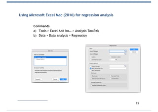
  • 6. Simple model • Regression analysis is the study of the relationship between one variable (the dependent variable, Y) and one or more other variables (independent variables, X) with a view to estimating and/or predicting the average value of the dependent variable (Y) in terms of known (or fixed) values of the independent ones (X) – We accumulate independent variables (X) to explain a dependent variable (Y) • Fitting a line to data means drawing a line that comes as close as possible to the points, providing a compact description of how X explains Y • In our case we are using changes in stores (X) to explain changes in sales (Y) 6
  • 7. Ordinary Least Squares: Introduction • Ordinary Least Squares (OLS) is a systematic method to construct the regression line • Since we wish to predict Y from X, we want a line that is as close as possible to the points in the vertical direction • We fit a line based on our past observations, in the expectation that they will help us predict future events • We have observations that give the real value of Y, and our regression line makes a prediction of Y (Y*). • We want to minimise the residual: Residual = observed value – predicted value 7An alternative method is to find an average no. of sales per store and multiply by 14. Since OLS will exaggerate the deviations it is a different method and therefore provides different results.
  • 8. 0 2,000 4,000 6,000 8,000 10,000 12,000 14,000 16,000 18,000 20,000 0 5 10 15 20 25 30 35 Sales Stores Graph 2 y e1 Y* (fitted value) Y (actual value) x e2 8 e3
  • 9. Ordinary Least Squares: Process • Take each observation (• ) and measure the deviation between the actual value (Y) and the fitted value (Y*) = (e1, e2, e3) • Every observation has a corresponding e – e2: squaring e will get rid of negative values, and give more weight to larger deviations – å e2: summing e2 takes into account all deviations – minå e2: make the fitted model as tight as possible to the sampled data by finding the minimum of the summed and squared values • Ordinary least squares (OLS) is a method of finding a* and b* such that the sum of squared residuals (å e2) is minimised 9 min $ 𝑒&
  • 10. y = 584.83x + 685.74 R² = 0.7455 0 2,000 4,000 6,000 8,000 10,000 12,000 14,000 16,000 18,000 20,000 0 5 10 15 20 25 30 35 Sales Stores Graph 3 Commands • Chart > Add Trendline… • Format Trendline > Options – Display equation on chart – Display R-squared value on chart 10
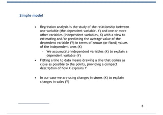
  • 11. Using Microsoft Excel (2003) for regression analysis Commands a) Tools > Add ins… > Analysis ToolPak b) Tools > Data analysis > Regression 11
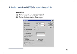
  • 12. Using Microsoft Excel (2007) for regression analysis Commands a) Office button > Excel options – Add ins > Manage > Excel add ins > Go – Analysis ToolPak > OK b) Data > Analysis > Data analysis 12
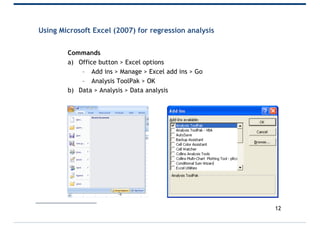
  • 13. Using Microsoft Excel Mac (2016) for regression analysis Commands a) Tools > Excel Add ins… > Analysis ToolPak b) Data > Data analysis > Regression 13
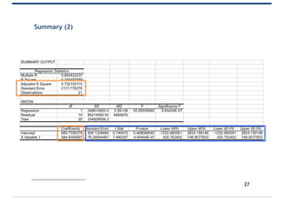
  • 14. Output 14 𝑦 = 𝑎 + 𝑏𝑥 s𝑎𝑙𝑒𝑠 = 𝑎 + 𝑏(𝑠𝑡𝑜𝑟𝑒𝑠) s𝑎𝑙𝑒𝑠 = 685.74 + 584.83(𝑠𝑡𝑜𝑟𝑒𝑠) ANOVA stands for “Analysis of Variance” which tests whether the means of different groups are equal. We do not need to use it for our purposes.
  • 15. 1. The board suspect that the country manager for Poland is underperforming. Based on the entire data set how many sales would you expect a location with 14 stores to generate? 15 𝑦 = 685.74 + 584.83𝑥 𝑦 = 685.74 + 584.83(14) 𝑦 = 8,873
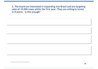
  • 16. 2. The board are interested in expanding into Brazil and are targeting sales of 10,000 cases within the first year. They are willing to invest in 8 stores – is this enough? 16 𝑦 = 685.74 + 584.83𝑥 10,000 = 685.74 + 584.83𝑥 10,000 − 685.74 584.83 = 𝑥 ∴ 𝑥 = 16
  • 17. Table 2 – a recap on how we generated a and b 17 Table 2 Y X Ŷ Ŷ-Y (Ŷ-Y)^2 Sales Stores Fitted Residual MSE 15,678 30 18,231 -2,552.64 6,515,971 16,758 22 13,552 3,206.00 10,278,436 4,895 8 5,364 -469.38 220,318 5,786 9 5,949 -163.21 26,638 12,323 16 10,043 2,279.98 5,198,309 9,870 10 6,534 3,335.96 11,128,629 5,436 8 5,364 71.62 5,129 6,754 7 4,780 1,974.45 3,898,453 7,863 9 5,949 1,913.79 3,662,592 4,659 8 5,364 -705.38 497,561 7,861 10 6,534 1,326.96 1,760,823 4,787 11 7,119 -2,331.87 5,437,618 5,567 14 8,873 -3,306.36 10,932,016 4,538 10 6,534 -1,996.04 3,984,176 7,859 8 5,364 2,494.62 6,223,129 5,489 6 4,195 1,294.28 1,675,161 3,436 6 4,195 -758.72 575,656 5,359 7 4,780 579.45 335,762 2,023 6 4,195 -2,171.72 4,716,368 1,434 5 3,610 -2,175.89 4,734,497 1,764 5 3,610 -1,845.89 3,407,310 Residual mean Mean Squared Error Y=685.74+584.83X 0.00 4,057,836
  • 18. Multiple R • r is a measure of the index of co-relation between two variables • Correlation – A number between -1 and +1 that indicates if two variables are linearly related – If r = 1 there is a perfectly positive relationship – If r = -1 there is a perfectly negative relationship – If r = 0 there is no (linear) relationship • If we only have a single independent variable R-squared will be equal to the square of the correlation between the dependent and independent variable. – In our case Multiple R = 0.863 and R-squared = 0.745 • We can also find r doing correlation analysis 18
  • 19. R-squared • r2 is the most commonly used goodness of fit for a regression line • It measures the proportion or percentage of the total variation in Y explained by the regression model • Hence 0 < r2 < 1 and the higher r2 the better – If r2 = 0 then there is no relationship between X and Y – If r2 = 1 then △X = △Y 19If we are comparing ice cream sales and wearing shorts we can imagine that r is high (more X = more Y) but r2 is low (△X /= △Y). Remember that correlation doesn’t mean causation!
  • 20. Adjusted R-squared • Adjusted r2 is a more precise measure of r2 since it takes into account the number of independent variables in the model • It only increases if a new variable improves the model 20 𝑟& = 1 − 𝑆𝐸& 𝑠& Note: here we’re using the SE of the error terms and the s of the dependent variable (Y)
  • 21. Standard error • The standard error is 2,117 – this is our estimate of the standard deviation of the residual error terms (i.e. how close the points are to the regression line) • If these errors are normally distributed – 68% of errors are within ± SE of the line – 95% of errors are within ± 2SE of the line – 99.7% of errors are within ± 3SE of the line • The lower the SE the better the fit • The SE gives an absolute measure of fit, r2 is a relative measure • r2 tells us how well the model does compared to our next best alternative – the values of Y 21Note: the standard error is the same unit of measurement as the dependent variable (Y). Notice that the standard error is ≈ the square root of the mean squared error.
  • 22. Table 3 – calculation for adjusted r2 Y X Ŷ Sales Stores Fitted 15,678 30 18,231 16,758 22 13,552 4,895 8 5,364 5,786 9 5,949 12,323 16 10,043 9,870 10 6,534 5,436 8 5,364 6,754 7 4,780 7,863 9 5,949 4,659 8 5,364 7,861 10 6,534 4,787 11 7,119 5,567 14 8,873 4,538 10 6,534 7,859 8 5,364 5,489 6 4,195 3,436 6 4,195 5,359 7 4,780 2,023 6 4,195 1,434 5 3,610 1,764 5 3,610 Mean 6,673.29 StDev 4,091.63 22 𝑟& = 1 − 𝑆𝐸& 𝑠& 𝑟& = 1 − 2117& 4091& 𝑟& = 1 − 4,481,689 16,736,281 𝑟& = 1 − 0.268 𝑟& = 0.732
  • 23. 3. How strong are stores as a predictor of sales? Adjusted r2 = 0.732 According to our model 73.2% of sales are determined by the number of stores 26.8% of sales are determined by other factors, which can be factored into our model to create a more robust picture 23
  • 25. Solutions 1. The board suspect that the country manager for Poland is underperforming. Based on the entire data set how many sales would you expect a location with 14 stores to generate? – 8,873 cases (compared to 5,567) 2. The board are interested in expanding into Brazil and are targeting sales of 10,000 cases within the first few years. They are willing to invest in 8 stores – is this enough? – No! They need around 16 stores 3. How strong are stores as a predictor of sales? – They explain over 70% 25
  • 26. Discussion questions • Issues of outliers – should we remove Germany? • Omitted variables – Marketing budget • Dangers of extrapolation – can we make estimates outside the range in which the data was constructed? • How can we improve on the model? – GDP per capita – No. of business trips per year 26
  • 28. Appendix The Excel output also gives the standard errors of the coefficients (given in brackets) t Stat • The estimated coefficient divided by the standard error • The distance between b and 0 (measured in units of the standard errors • It’s how many standard errors the estimate is from 0 P value • The probability of seeing a t stat that big (or bigger) if β = 0 • There is a 0.00000046 chance of a t stat bigger than 7.46 The t stat is large (and the p value small) so we are confident that β > 0, i.e. that the number of stores have a positive effect on sales We may wish to perform a test against a more reasonable hypothesis (e.g. β = 500) Note: we use a t-stat instead of a z score because of the low sample size, but the intuition is identical 28 (926) (78.39) 𝑦 = 685.74 + 584.83𝑥