Basic MATLAB Programming PPT.pptx

What is MATLAB?
⚫MA
TLAB(short for MA
Trix LABoratory) is aspecial-
purpose computer program optimized to perform
engineering and scientific calculations.
⚫It started life asaprogram designed to perform matrix
mathematics.
⚫Over the years, it hasgrowninto aflexiblecomputing
system capable of solving essentially anytechnical problem.
⚫The MA
TLABprogram implements the MA
TLAB
programming language and provides an extensive library of
predefined functions to make technical programming tasks
easier and more efficient.
[Chapman, 2013]
2

Command Window
⚫ MA
TLABexpressions and statements are evaluated as you
execute them in the Command Window, and results of the
computation are displayed there too.
⚫Command-line interface: a means of interacting with a computer
program where the user (or client) issues commands to the program
in the form of successive lines of text (command lines).
the prompt
3

MATLAB Command Window
5
⚫ MA
TLABexpressions and statements are evaluated as you
execute them in the Command Window, and results of the
computation are displayed there too.
⚫Command-line interface: a means of interacting with a computer
program where the user (or client) issues commands to the program
in the form of successive lines of text (command lines).
⚫ Forms:
or simply:
variable = expression
expression
⚫ Ifthe variable name and = sign are omitted,avariable ans (for
answer) is automatically created to which the result is assigned.
⚫This default variable is reused anytime onlyan expression is typed at
the prompt.
the assignment operator
(unlike in
mathematics, the
single equal sign does
not mean equality)

Using MATLAB as a Calculator
⚫ In its simplest form, MA
TLABcan be used asacalculator to perform
mathematical calculations.
⚫ The calculations to be performed are typed directly into the Command
Window,usingthe symbols+, -, *, /, and^ for addition, subtraction,
multiplication, division,and exponentiation,respectively.
⚫ After an expression is typed, the results of the expression will be
automatically calculated and displayed.
⚫ If an equal sign is used in the expression, then the result of the
calculation is saved in the variable name to the left of the equal sign.
5

Constants
⚫ There is no built-in constant for e
(2.718). Use the exponential function
exp; e or e1 is equivalent to exp(1).
⚫ Don’t confuse the value ewith the e
used in MA
TLABto specify anexponent
for scientific notation.
6

MATLAB desktop
⚫ The Workspace window lists variables that you haveeither entered or
computed in your MA
TLABsession.
⚫ Use the up and down arrows to scroll through the stack of previous commands.
⚫ Re-execute one more commands from the Command History window by
(1)double-clickingor (2) draggingthe command(s) into the Command
Window or (3) selecting the commands and then right-click to bring up the
menu.
7

Valid Names
⚫Start with aletter, followed byletters, digits, or
underscores.
⚫Cannot have aspace
⚫MA
TLABis case-sensitive in the names of commands,
functions, and variables.
⚫A and a are two different variables.
⚫Y
oucannot define variables with the same names asMA
TLAB
keywords(reserved words), such as if or end.
⚫For acomplete list, run the iskeyword command.
⚫Namesof built-in functions can,but should not, be used as
variable names.
8

Matrix
⚫ MA
TLAB= matrix laboratory
⚫ There are manyfundamental data types (or classes) in
MA
TLAB, each one amultidimensional array.
⚫Individual data values within an array can be accessed byincluding the
name of the array followed by subscripts in parentheses that identify
the location of the particular value.
⚫ The classesyou will use most are rectangular numerical arrays
with possibly complex entries,and possibly sparse.
⚫ An arrayof thistype is called amatrix.
⚫ Amatrix with onlyone row or one column is called avector.
⚫ A1-by-1 matrix is calledascalar.
9

Matrix
11
⚫The figure on the right shows two
commands which creates a 3-by-3
matrix and assigns it to a variable
A.
⚫Acomma or blankseparates the
elements within arow ofa matrix.
⚫Asemicolon endsarow
.
⚫Double-clicking
on avariable in
theW
orkspace
window pulls
up the V
ariable
Editor.

Referring to and Modifying Elements
11

Array Operations
⚫ MA
TLABsupports two types of
operations between arrays,known as
arrayoperations and matrix operations.
⚫ Array operations are operations
performed between arrayson an
element-by-element basis.
⚫Note that for these operations to work,
the number of rows and columns in both
arraysmust be the same.
⚫ Ifthe arrayoperation is performed
between an arrayand a scalar, the
value of the scalar is applied to every
element of the array
.
12

Matrix Operations
⚫Matrix operations follow the normal rules
of linear algebra, such asmatrix multiplication.
⚫MA
TLABuses aspecial symbol to distinguish
arrayoperationsfrom matrix operations.
⚫Inthe cases where arrayoperationsand matrix
operationshave adifferent definition, MA
TLAB
uses aperiod before the symbol to indicate an
arrayoperation (for example, * vs. .*).
13

Common Array and Matrix Operations
15
[Chapman, 2013,T
able 2-6]

Ex. Generating a Sequence of Coin
Tosses
⚫Use 1 to represent Heads;0 to representT
ails
⚫rand(1,120) < 0.5
15

rand function: a preview
⚫Generate an arrayof uniformly
distributed pseudorandom numbers.
⚫The pseudorandomvalues are drawn
from the standard uniform
distribution on the open interval
(0,1).
⚫rand returns ascalar.
⚫rand(m,n) or rand([m,n])
returns an m-by-nmatrix.
⚫rand(n) returns an n-by-nmatrix
16

hist function
⚫ Create histogram plot
⚫ hist(data) creates a histogram bar plot of data.
⚫ Elements in data are sorted into 10 equally spaced bins along the x-axis
between the minimum and maximum valuesof data.
⚫ Binsare displayedasrectangles such that the height of each rectangle
indicates the number of elements in the bin.
⚫ Ifdata is avector,then one histogram is created.
⚫ Ifdata is amatrix,then ahistogram is created separately for each column.
⚫ Eachhistogram plot is displayed on the same figure with adifferentcolor.
⚫ hist(data,nbins) sorts data into the number of bins specified
bynbins.
⚫ hist(data,xcenters)
⚫ The valuesin xcenters specifythe centers for each bin on the x-axis.
17

hist function: Example
1.5 2 2.5 3 3.5 4 4.5 5
0
1
2
1.8
1.6
1.4
1.2
1
0.8
0.6
0.4
0.2
10
The width of each bin is 5 1
 0.4
min
max
18

rand function: Histogram
⚫Thegeneration isunbiased in the sensethat “anynumber in
the range is as likely to occur asanother number.”
⚫Histogram is flat over the interval (0,1).
0.1 0.2 0.3 0.4 0.5 0.6 0.7 0.8 0.9 1
0
0
5
10
15
0.1 0.2 0.3 0.4 0.5 0.6 0.7 0.8 0.9 1
0
0
2
4
6
8
10
hist(rand(1,100))
19
hist(rand(1,1e6))
4
x 10
12
Roughly
the same
height

randn function: a preview
-6 -4 -2 0 2 4 6
2
1.8
1.6
1.4
1.2
1
0.8
0.6
0.4
0.2
0
x 10
5
⚫Generate an array of normally distributed pseudorandom
numbers
hist(randn(1,1e6),20)
20

Relational Operators
⚫ Perform element-by-element comparisons
between two arrays.
⚫ Return alogicalarrayof the same size,
with elements set to logical 1 (true)
where the relation is true, and elements set
to logical 0 (false) where it is not.
⚫ If one of the operands is a scalar and the
other a matrix, the scalar expands to the
size of the matrix.
21

Ex. Generating a Sequence of 120 Coin
Tosses
⚫Use 1 to represent Heads;0 to representT
ails
⚫rand(20,6) < 0.5 Arrangethe results in a20×6 matrix.
22

Randomness
⚫Manyclever people havethought about and debated what
randomnessreally is, andwecouldget into along
philosophical discussion.Let’s not.
⚫The French mathematician Laplace(1749–1827) put it
nicely:“Probability is composed partly of our ignorance,
partlyof our knowledge.”
⚫Inspired byLaplace,let us agree that you can use probabilities
whenever you are faced with uncertainty
.
23

Sources of Randomness
Random phenomenaarise because of:
⚫our partial ignorance of the generating mechanism
⚫the laws governing the phenomena maybe fundamentally
random (as in quantum mechanics)
⚫our unwillingness to carryout exact analysis becauseit is not
worth the trouble
24

AGlimpse at Probability Theory
⚫Probabilities are used in situations that involve randomness.
⚫Aprobability is anumber used to describe how likely
something is to occur,and probability (without indefinite
article) is the studyof probabilities.
⚫It is“the art of being certain of how uncertain youare.”
⚫Ifan event is certain to happen,it is given aprobability of 1.
Ifit is certain not to happen, it has aprobability of 0.
25

Ingredients of Probability Theory
⚫ Anactivityor procedure or observation iscalledarandom
experiment if its outcome cannot be predicted precisely because
the conditions under which it is performed cannot be
predetermined with sufficient accuracyand completeness.
⚫ Arandom experiment mayhaveseveralseparatelyidentifiable
outcomes.We definethe sample space Ω asacollection ofall
possible (separately identifiable) outcomes/results/measurements
of arandomexperiment.
⚫ Eachoutcome (ω) is anelement, or sample point, of thisspace.
⚫ Events are sets(or classes) of outcomes meeting some
specifications.
⚫ The goal of probability theory is to compute the probability of
variousevents of interest.
26

“Being certain of how uncertain you are”
⚫ The statement“whenacoin is tossed,the probability to get heads
is l/2 (50%)”is aprecise statement.
⚫ It tells you that you are aslikely to get heads asyou are to get tails.
⚫ Another wayto think about probabilities is in terms of average
long-term behavior.
⚫ Ifyou toss the coin repeatedly, in the long run you will get
“roughly”50%headsand 50%tails.
⚫ Even more precise statement/interpretation can be made using
the law of large numbers.
⚫ Although the outcome of arandom experiment is unpredictable,
there is astatistical regularity about the outcomes.
⚫What you cannot be certain of is how the next toss will come up.
27

Long-run frequency interpretation
⚫ Ifthe probability P(A)of an eventAin some actual physical
experiment is p,
then, bythe law of large numbers (LLN),
if the experiment is repeated independently over and over
again, then, in the longrun, the eventAwill happen
“approximately”100p%of the time.
In the limit,the fraction of times that eventAoccurs will converge
to 100p%.
⚫ In other words,if we repeat an experiment alarge number of
times then the fraction of times that eventAoccurs will be close
to P(A).
⚫This fraction of times is called the relative frequency of the event
A.
⚫So, LLNsimply saysthat the relative frequency will converge to the
actual probability when we repeat an experiment a large number of
times.
28

Coin Tossing: Relative Frequency
2 4 6 8 10
0.2
0
1
0.8
0.6
0.4
0
0.2
0.4
0.6
0.8
1
20 40 60 80 100
0
0.2
0.4
0.6
0.8
1
2 6 8 10
x 10
5
0
0.2
0.4
0.6
0.8
1
n 1,2, ,10 ,100
n 1,2,
200 400 600 800 1000
,1000
n 1,2,
4
n 1,2, ,106
Ifafair coin is
flipped alarge
number of times,
the proportion of
headswill tend to
get closer to 1/2 as
the number of
tosses increases.
29

Coin Tossing: Relative Freq. vs. #H-#T
Ifafair coin is
flipped alarge
number of times,
the proportion of
headswill tend to
get closer to 1/2 as
the number of
tosses increases.
This statement does not saythat the
difference between #H and #T will be
close to 0.
1 2 3 4 6 7 8 9 10
x 10
5
-500
0
500
1000
1500
2000
2500
The difference
between #H and
#T will not
converge to 0.
30
5
n

Another Simulation
2 4 6 8 10
1
0.8
0.6
0.4
0.2
0
600 800 1000
0
0.2
0.4
0.6
0.8
1
0
0.2
0.4
0.6
0.8
0
0.2
0.4
0.6
0.8
1
1 2 3 4 5 6 7 8 9 10
x 10
5
-600
-400
-200
0
200
400
600
800
Relative Freq.
1 1000
31
# H-#T
n
n
200 400
n 2 4
n 6 8 10
x 10
5
20 40
n 60 80 100

Another Simulation
2 4 6 8 10
1
0.8
0.6
0.4
0.2
0
200 400 600 800 1000
0
0.2
0.4
0.6
0.8
1
0
0.2
0.4
0.6
0.8
1
2 4 6 8
0
0.2
0.4
0.6
0.8
1
1 2 3 4 5 6 7 8 9 10
x 10
5
10 -600
x 10
5
-500
-400
-300
-200
100-100
0
100
200
300
Relative Freq.
32
# H-#T
n
n
n n
20 40 60 80
n

MATLAB Code: Scripts and Functions
⚫ M-files
⚫ Y
oucan write aseries of commands to afile that you then execute
as you would anyMA
TLABfunction.
⚫Use the MA
TLABEditor or anyother text editor to create your own
function files.
⚫Call these functions asyou would anyother MA
TLABfunction or
command.
⚫ There are two kindsof program files:
1. Scripts: do not accept input arguments or return output
arguments.
2. Functions: can accept input arguments and return output
⚫ If you duplicate function names, MA
TLABexecutes the one that
occursfirst in itssearchpath.
33

MATLAB Search Path
⚫MA
TLABhasasearchpath that it uses to find M-files.
⚫Manydirectories of M-files are alreadyincluded.
⚫Usersmayadd others. .
⚫Ifauser enters anameat the MA
TLABprompt, the
MA
TLABinterpreter attempts to find the name asfollows:
1. It looks for the name asavariable.If it is avariable,MA
TLAB
displaysthe current contents of the variable.
2. It checks to see if the name is an M-file in the current directory.
Ifit is,MA
TLABexecutes that function or command.
3. It checks to see if the name is an M-file in any directory in the
searchpath. Ifit is, MA
TLABexecutes that functionor
command.
34

MATLAB Search Path
⚫ Caution: Never use avariable with the same
name asaMA
TLABfunction or command.
⚫MA
TLABchecks for variable names first, so
if you define avariable with the same name
as aMA
TLABfunction or command, that
function or command becomes inaccessible.
⚫ Ifthere is more than one function or command with the same
name, the first one found on the searchpath will be executed,and
all of the otherswill be inaccessible.
⚫ Never create an M-file with the same name asaMA
TLABfunction
or command.
⚫This is acommon problem for novice users,since they sometimes
create M-files files with the same names asstandard MA
TLAB
functions, making them inaccessible.
⚫ Function exist returns 0 if there are no existing variables,
functions, or other artifacts with the proposed name.
35

MATLAB Scripts
⚫Simplyexecute the commands found in the file.
⚫Can operate on existing data in the workspace
⚫Can create new data on which to operate.
⚫Can produce graphical output using functions like plot.
⚫Although they do not return output arguments, anyvariables
that they create remain in the workspace,to be used in
subsequent computations.
36

Clear, clc
⚫ clear: Clear variables and functions from memory.
⚫clear removes all variablesfrom the workspace.
⚫clearV
ARIABLESdoes the same thing.
⚫ Alternatively,right-clicking the variable in theWorkspace window and
selectingDelete.
⚫clear GLOBALremoves all global variables.
⚫clear FUNCTIONS removes all compiled MA
TLABand
MEX-functions.
⚫clear ALL removes all variables,globals,functions and
MEXlinks.
⚫close ALL closes all the open figure windows.
37

Semicolon and Statement Termination
⚫Astatement is normally terminated at the end of the line.
⚫However,astatement can be continued to the next line with
three periods (...) at the end of the line.
⚫Several statements can be placed on asingle line separated by
commas or semicolons.
⚫Ifthe last character of a statement is asemicolon, display of
the result is suppressed, but the assignment is still carried
out.
⚫This is essentialin suppressing unwanted displayof intermediate
results (which usuallyslow down the computation).
38

plot function
⚫ Create 2-D line plot
⚫ plot(Y) plots (vector) Y versus the index of each value.
⚫If Y is a matrix, plot(Y) plots the columns of Y versus the
index of each value.
⚫ plot(X1,Y1,...,Xn,Yn) plots each vector Yn versus
vector Xn on the same axes.
⚫If one of Yn or Xn is a matrix and the other is a vector, it plots the
vector versus the matrix row or column with a matching dimension
to the vector.
⚫If Xn is ascalar and Yn is avector,it plots discrete Yn points
vertically at Xn.
⚫If Xn or Yn are matrices, they must be 2-D and the same size,and
the columns of Yn are plotted against the columns of Xn.
39

plot function: Example
Click here to show PlotT
ools
40

hold function
42
⚫Control whether MA
TLABclears the
current graph when you make subsequent
calls to plotting functions (the default), or
addsanew graph to the current graph.
⚫hold on retains the current graph and
addsanother graph to it.
⚫hold off resets hold state to the default
behavior, in which MA
TLABclearsthe
existing graph and resets axes properties to
their defaults before drawing new plots.
1 1.5 2 2.5 3 3.5 4
1
3.5
3
2.5
2
1.5
4
4.5
5

sum function
⚫ Calculate the sum of arrayelements
⚫ sum(A) returns sums along different dimensions
of an array
.
⚫ IfA is avector, sum(A) returns the sum of the
elements.
⚫ IfA is amatrix, sum(A)treats the columnsof A as
vectors, returningarow vector of the sums of each
column.
⚫ sum(A,dim) sums alongthe dimension of A
specified byscalar dim.
⚫Set dim to
⚫ 1 to compute the sum of each column,
⚫ 2 to sum rows, etc.
42

cumsum function
⚫Calculate the cumulative sum
⚫If A is a vector, cumsum(A) returns a
vector containing the cumulative sum of
the elementsofA.
⚫IfA is amatrix, cumsum(A)returns a
matrix containing the cumulative sums for
each column ofA.
⚫cumsum(A,dim) returns the
cumulative sum of the elements along
dimension dim.
43

Creating equally spaced vectors
⚫ The colon operator
⚫ j:k is the same as[j,j+1,...,k]
⚫a:d:b produces an array that starts at a, advances in increments of
d, and ends when the last point plus the increment would equal or
exceed the value b.
⚫ Twodisadvantages of the colon operator:
⚫It is not alwayseasy to know how many points will be in the array.
⚫There is no guarantee that the last specified point will be in the array,
since the increment could overshoot that point.
44

Creating equally spaced vectors
⚫The linspace function generates linearly spaced vectors.
⚫Similar to the colon operator,but give direct control over the
number of points.
⚫linspace(a,b,n) generates arow vector yof n points
linearlyspacedbetween and includingaand b.
45

Referring to and Modifying Elements:
A Revisit
46

Capturing figure
close all; clear all;
N = 1e3; % Number of trials (number of times that the coin is tossed)
s = (rand(1,N) < 0.5); % Generate a sequence of N Coin Tosses.
% The results are saved in a row vector s.
NH = cumsum(s); % Count the number of heads
plot(NH./(1:N)) % Plot the relative frequencies
LLN_cointoss.m
47

Exercise
⚫Modify the script
LLN_cointoss.m so
that it alsoshows the
relative frequencies for
the tails event.
⚫The plot command that
you added to the script
should alsospecify the
color of the graph for the
tails event to be red. (Use
the help or doc command
to learn more about the
plot function.)
100 200 300 400 500 600 700 800 900 1000
0
0
0.1
0.2
0.3
0.4
0.5
0.6
0.7
0.8
0.9
1
49

randi function
⚫ Generate uniformly distributed pseudorandom integers
⚫ randi(imax,m,n) and randi(imax,[m,n]) return
an m-by-nmatrix of numbers.
⚫ randi(imax,n) returns an n-by-nmatrix containing
pseudorandom integer values drawn from the discrete uniform
distributionon the interval [1,imax].
⚫ randi(imax) returns ascalar value between 1 and imax.
⚫This is the same as randi(imax,1).
⚫ randi([imin,imax],...) returns an arraycontaining
integer values drawn from the discrete uniform distribution on the
interval [imin,imax].
50

randi function: Example
s = (rand(1,N) < 0.5); % Generate a sequence of N Coin Tosses.
% The results are saved in a row vector s.
NH = cumsum(s); % Count the number of heads
plot(NH./(1:N)) % Plot the relative frequencies
LLN_cointoss.m
Same as
randi([0,1],1,N);
51

The word “dice”
⚫Historically,dice is the plural of die.
⚫In modern standard English,dice is used asboth the
singular and the plural.
Example of 19th Centurybone dice
52

“Advanced” dice
[http://gmdice.com/ ]
53

Dice Simulator
⚫http://www.dicesimulator.com/
⚫Support up to 6 dice and alsohassome background
information on dice and random numbers.
54

Classical Probability
⚫ Assumptions
⚫The number of possible outcomes is finite.
⚫Equipossibility:The outcomes have equal probability of
occurrence.
⚫ Equi-possible;equi-probable; euqally likely;fair
⚫ The bases for identifyingequipossibility were often
⚫ physical symmetry (e.g. awell-balanced die, made of homogeneous
material in acubical shape)
⚫ abalance of information or knowledge concerning the various possible
outcomes.
⚫ Formula:Aprobabilityis a fraction in which the bottom
represents the number of possible outcomes,while the number on
top represents the number of outcomes in which the event of
interest occurs.
57

Two Dice
59
⚫Apair of dice
Double six

Two dice: Simulation
[ http://www2.whidbey.net/ohmsmath/webwork/javascript/dice2rol.htm ]
59

Two dice
⚫Assume that the two dice are fair and independent.
⚫P[sumof the two dice = 5] = 4/36
60

Two dice
⚫Assume that the two dice are fair and independent.
61

Leibniz’s Error (1768)
64
⚫Though one of the finest minds of his age,Leibniz wasnot
immune to blunders:he thought it just aseasyto throw 12
with apair of dice asto throw 11.
⚫The truth is...
⚫Leibniz is aGerman philosopher, mathematician,
and statesman who developed differential and
integral calculus independentlyof Isaac Newton.
36
1
36
P[sum of the two dice = 11] 
2
P[sum of the two dice = 12] 
[Gorroochurn, 2012]
0
0 100 200 300 400 500 600 700 800 900 1000
0.05
0.1
0.15
0.2
0.25

Loops
65
⚫Loops are MA
TLABconstructs that permit us to execute a
sequence of statements more than once.
⚫There are two basic forms of loop constructs:
⚫while loops and
⚫for loops.
⚫The major difference between these two types of loops is in
how the repetition is controlled.
⚫The code in awhile loop is repeated an indefinite number of
times until some user-specifiedcondition is satisfied.
⚫Bycontrast, the code in afor loop is repeated aspecified
number of times, and the number of repetitions is known
before the loops starts.

for loop: a preview
66
⚫ Execute ablockof statements aspecified number of
times.
⚫ k is the loop variable (also known as the loop
index or iterator variable).
⚫ expr is the loop control expression, whose result
usuallytakes the form of avector.
⚫The elements in the vector are stored one at atime in the
variable k, and then the loop body is executed, so that
the loop is executed once for each element in the array
produced byexpr.
⚫ The statements between the for statement and the end
statement are known as the body of the loop.They are
executed repeatedlyduring each pass of the for loop.
for k = expr
body
end
for_ex1.m
for k = 1:5
x = k
end

Another Version of the Old Example
LLN_cointoss_for.m
%% Preallocation
s = zeros(1,N);
NH = zeros(1,N);
RF = zeros(1,N);
S(1) = randi([0,1]);
NH(1) = s(1);
RF(1) = NH(1)/1;
for k = 2:N
s(k) = randi([0,1]);
NH(k) = NH(k-1)+s(k);
RF(k) = NH(k)/k;
end
plot(RF) % Plot the relative frequencies
66

Preallocating Vectors
⚫ When the content of avector is computed/added/known
⚫ One method is to start with an empty vector and extend the vector by adding
each number to it asthe numbers are entered bythe user.
⚫ Extending avector,however,is very inefficient.What happens isthat every time
avector is extended anew“chunk”of memorymust be found that islarge
enough for the new vector,and all of the values must be copied from the
original location in memory to the new one.This can take along time.
⚫ Abetter method isto preallocate the vector to the correct size and then change
the valueof each element to store the desired value.
⚫ This method involvesreferring to each index in the output vector,and placing
each number into the next element in the output vector.
⚫ This method is far superior,if it is known aheadof time how manyelements the
vector will have.
⚫ One common method isto use the zerosfunction to preallocate the vector to
the correct length.
67

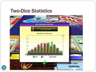
Exercise
⚫ Write MA
TLABscript to
simulate repeated rolls of two
dices.
⚫ Calculate the sum of the two
dices.
⚫ Plot the relative frequencyfor
the event that the sum is 11.
⚫ In the same figure, plot (in red)
the relative frequencyfor the
event that the sum is 12.
⚫ In another figure, create a
histogramfor the sum after 130
roll of two dice.
100 200 300 400 500 600 700 800 900 1000
0
0
0.05
0.1
0.15
0.2
0.25
2 3 4 5 6 7 8 9 10 11 12
0
5
10
15
20
25
68

Scandal of Arithmetic
70
Which is more likely
, obtaining at least one
six in 4 tosses ofafair dice (event A), or
obtaining at least one double six in 24 tosses
of apair of dice (event B)?
64
64
3624
3624
54
 5 
4
P(A)  1 6   .518
 
3524
 35 
24
P(B)  1 36   .491
 
[http://www.youtube.com/watch?v=MrVD4q1m1Vo]

“Origin” of Probability Theory
71
⚫Probability theory wasoriginally inspired by gambling
problems.
⚫In1654, Chevalierde Méréinvented agamblingsystem
which bet even moneyon caseB.
⚫When he began losingmoney
, he asked his mathematician
friend Blaise Pascal to analyze his gamblingsystem.
⚫Pascal discovered that the Chevalier's system would lose
about 51 percent ofthe time.
⚫Pascal became so interested in probability and together with
another famous mathematician, Pierre de Fermat, they laid
the foundation of probabilitytheory
.
best known for Fermat's LastTheorem

Basic MATLAB Programming PPT.pptx

More Related Content

What's hot (20)

Similar to Basic MATLAB Programming PPT.pptx (20)

Recently uploaded (20)

Basic MATLAB Programming PPT.pptx