Lesson 14: Exponential Functions
0 likes270 views

This document defines and explains exponential functions. It begins by defining an as a positive whole number and discusses properties like ax+y = ax * ay. It introduces conventions to define exponential functions for non-positive whole number exponents, like defining a0 = 1 and a-n = 1/an. It discusses graphs of various exponential functions and limits of exponential functions as x approaches positive or negative infinity. The document then discusses the natural exponential function and introduces the number e through the concept of compound interest calculations.


![Compounded Interest: continuous
Question
Suppose you save P at interest rate r, with interest compounded
every instant. How much do you have after t years?
Answer
( ( )
r )nt 1 rnt
B(t) = lim P 1 + = lim P 1 +
n→∞ n n→∞ n
[ ( )n ]rt
1
= P lim 1 +
n→∞ n
independent of P, r, or t
. . . . . .](https://image.slidesharecdn.com/lesson14-exponentialfunctions034slides-091022085533-phpapp02/85/Lesson-14-Exponential-Functions-55-320.jpg)


Lesson 14: Exponential Functions
- 1. Section 3.1 Exponential Functions V63.0121.034, Calculus I October 19, 2009 . . . . . .
- 2. Outline Definition of exponential functions Properties of exponential Functions The number e and the natural exponential function Compound Interest The number e A limit . . . . . .
- 3. Definition If a is a real number and n is a positive whole number, then an = a · a · · · · · a n factors . . . . . .
- 4. Definition If a is a real number and n is a positive whole number, then an = a · a · · · · · a n factors Examples 23 = 2 · 2 · 2 = 8 34 = 3 · 3 · 3 · 3 = 81 (−1)5 = (−1)(−1)(−1)(−1)(−1) = −1 . . . . . .
- 5. Fact If a is a real number, then ax+y = ax ay ax ax−y = y a (ax )y = axy (ab)x = ax bx whenever all exponents are positive whole numbers. . . . . . .
- 6. Fact If a is a real number, then ax+y = ax ay ax ax−y = y a (ax )y = axy (ab)x = ax bx whenever all exponents are positive whole numbers. Proof. Check for yourself: a x +y = a · a · · · · · a = a · a · · · · · a · a · a · · · · · a = a x a y x + y factors x factors y factors . . . . . .
- 7. Let’s be conventional The desire that these properties remain true gives us conventions for ax when x is not a positive whole number. . . . . . .
- 8. Let’s be conventional The desire that these properties remain true gives us conventions for ax when x is not a positive whole number. For example: a n = a n +0 = a n a 0 ! . . . . . .
- 9. Let’s be conventional The desire that these properties remain true gives us conventions for ax when x is not a positive whole number. For example: a n = a n +0 = a n a 0 ! Definition If a ̸= 0, we define a0 = 1. . . . . . .
- 10. Let’s be conventional The desire that these properties remain true gives us conventions for ax when x is not a positive whole number. For example: a n = a n +0 = a n a 0 ! Definition If a ̸= 0, we define a0 = 1. Notice 00 remains undefined (as a limit form, it’s indeterminate). . . . . . .
- 11. Conventions for negative exponents If n ≥ 0, we want an · a−n = an+(−n) = a0 = 1 ! . . . . . .
- 12. Conventions for negative exponents If n ≥ 0, we want an · a−n = an+(−n) = a0 = 1 ! Definition 1 If n is a positive integer, we define a−n = . an . . . . . .
- 13. Conventions for negative exponents If n ≥ 0, we want an · a−n = an+(−n) = a0 = 1 ! Definition 1 If n is a positive integer, we define a−n = . an Fact 1 The convention that a−n = “works” for negative n as well. an am If m and n are any integers, then am−n = n . a . . . . . .
- 14. Conventions for fractional exponents If q is a positive integer, we want (a1/q )q = a1 = a ! . . . . . .
- 15. Conventions for fractional exponents If q is a positive integer, we want (a1/q )q = a1 = a ! Definition √ If q is a positive integer, we define a1/q = q a. We must have a ≥ 0 if q is even. . . . . . .
- 16. Conventions for fractional exponents If q is a positive integer, we want (a1/q )q = a1 = a ! Definition √ If q is a positive integer, we define a1/q = q a. We must have a ≥ 0 if q is even. Fact Now we can say ap/q = (a1/q )p without ambiguity . . . . . .
- 17. Conventions for irrational powers So ax is well-defined if x is rational. What about irrational powers? . . . . . .
- 18. Conventions for irrational powers So ax is well-defined if x is rational. What about irrational powers? Definition Let a > 0. Then ax = lim ar r→x r rational . . . . . .
- 19. Conventions for irrational powers So ax is well-defined if x is rational. What about irrational powers? Definition Let a > 0. Then ax = lim ar r→x r rational In other words, to approximate ax for irrational x, take r close to x but rational and compute ar . . . . . . .
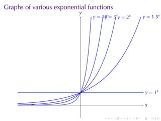
- 20. Graphs of various exponential functions y . . x . . . . . . .
- 21. Graphs of various exponential functions y . . = 1x y . x . . . . . . .
- 22. Graphs of various exponential functions y . . = 2x y . = 1x y . x . . . . . . .
- 23. Graphs of various exponential functions y . . = 3x. = 2x y y . = 1x y . x . . . . . . .
- 24. Graphs of various exponential functions y . . = 10x= 3x. = 2x y y . y . = 1x y . x . . . . . . .
- 25. Graphs of various exponential functions y . . = 10x= 3x. = 2x y y . y . = 1.5x y . = 1x y . x . . . . . . .
- 26. Graphs of various exponential functions y . . = (1/2)x y . = 10x= 3x. = 2x y y . y . = 1.5x y . = 1x y . x . . . . . . .
- 27. Graphs of various exponential functions y . y y . = x . = (1/2)x (1/3) . = 10x= 3x. = 2x y y . y . = 1.5x y . = 1x y . x . . . . . . .
- 28. Graphs of various exponential functions y . y y . = x . = (1/2)x (1/3) . = (1/10)x. = 10x= 3x. = 2x y y y . y . = 1.5x y . = 1x y . x . . . . . . .
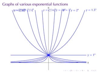
- 29. Graphs of various exponential functions y . yy = 213)x . . = ((//2)x (1/3)x y . = . = (1/10)x. = 10x= 3x. = 2x y y y . y . = 1.5x y . = 1x y . x . . . . . . .
- 30. Outline Definition of exponential functions Properties of exponential Functions The number e and the natural exponential function Compound Interest The number e A limit . . . . . .
- 31. Properties of exponential Functions Theorem If a > 0 and a ̸= 1, then f(x) = ax is a continuous function with domain R and range (0, ∞). In particular, ax > 0 for all x. If a, b > 0 and x, y ∈ R, then ax+y = ax ay ax ax−y = y a (ax )y = axy (ab)x = ax bx Proof. This is true for positive integer exponents by natural definition Our conventional definitions make these true for rational exponents Our limit definition make these for irrational exponents, too . . . . . .
- 32. Properties of exponential Functions Theorem If a > 0 and a ̸= 1, then f(x) = ax is a continuous function with domain R and range (0, ∞). In particular, ax > 0 for all x. If a, b > 0 and x, y ∈ R, then ax+y = ax ay ax ax−y = y negative exponents mean reciprocals. a (ax )y = axy (ab)x = ax bx Proof. This is true for positive integer exponents by natural definition Our conventional definitions make these true for rational exponents Our limit definition make these for irrational exponents, too . . . . . .
- 33. Properties of exponential Functions Theorem If a > 0 and a ̸= 1, then f(x) = ax is a continuous function with domain R and range (0, ∞). In particular, ax > 0 for all x. If a, b > 0 and x, y ∈ R, then ax+y = ax ay ax ax−y = y negative exponents mean reciprocals. a (ax )y = axy fractional exponents mean roots (ab)x = ax bx Proof. This is true for positive integer exponents by natural definition Our conventional definitions make these true for rational exponents Our limit definition make these for irrational exponents, too . . . . . .
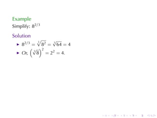
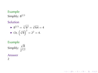
- 34. Example Simplify: 82/3 . . . . . .
- 35. Example Simplify: 82/3 Solution √ 3 √ 8 2 /3 = 82 = 3 64 = 4 . . . . . .
- 36. Example Simplify: 82/3 Solution √3 √ 82/3 = 82 = 64 = 4 3 (√ )2 8 = 22 = 4. 3 Or, . . . . . .
- 37. Example Simplify: 82/3 Solution √3 √ 82/3 = 82 = 64 = 4 3 (√ )2 8 = 22 = 4. 3 Or, Example √ 8 Simplify: 1/2 2 . . . . . .
- 38. Example Simplify: 82/3 Solution √3 √ 82/3 = 82 = 64 = 4 3 (√ )2 8 = 22 = 4. 3 Or, Example √ 8 Simplify: 1/2 2 Answer 2 . . . . . .
- 39. Fact (Limits of exponential functions) y . . = (= 2()1/3)x3)x y . 1/=x(2/ y y . . = (. /10)10x = 2x. = y y = x . 3x y y y 1 . = If a > 1, then lim ax = ∞ and x→∞ lim ax = 0 x→−∞ If 0 < a < 1, then lim ax = 0 and y . = x→∞ lim ax = ∞ . x . x→−∞ . . . . . .
- 40. Outline Definition of exponential functions Properties of exponential Functions The number e and the natural exponential function Compound Interest The number e A limit . . . . . .
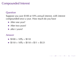
- 41. Compounded Interest Question Suppose you save $100 at 10% annual interest, with interest compounded once a year. How much do you have After one year? After two years? after t years? . . . . . .
- 42. Compounded Interest Question Suppose you save $100 at 10% annual interest, with interest compounded once a year. How much do you have After one year? After two years? after t years? Answer $100 + 10% = $110 . . . . . .
- 43. Compounded Interest Question Suppose you save $100 at 10% annual interest, with interest compounded once a year. How much do you have After one year? After two years? after t years? Answer $100 + 10% = $110 $110 + 10% = $110 + $11 = $121 . . . . . .
- 44. Compounded Interest Question Suppose you save $100 at 10% annual interest, with interest compounded once a year. How much do you have After one year? After two years? after t years? Answer $100 + 10% = $110 $110 + 10% = $110 + $11 = $121 $100(1.1)t . . . . . . .
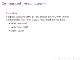
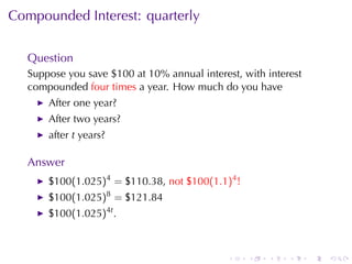
- 45. Compounded Interest: quarterly Question Suppose you save $100 at 10% annual interest, with interest compounded four times a year. How much do you have After one year? After two years? after t years? . . . . . .
- 46. Compounded Interest: quarterly Question Suppose you save $100 at 10% annual interest, with interest compounded four times a year. How much do you have After one year? After two years? after t years? Answer $100(1.025)4 = $110.38, . . . . . .
- 47. Compounded Interest: quarterly Question Suppose you save $100 at 10% annual interest, with interest compounded four times a year. How much do you have After one year? After two years? after t years? Answer $100(1.025)4 = $110.38, not $100(1.1)4 ! . . . . . .
- 48. Compounded Interest: quarterly Question Suppose you save $100 at 10% annual interest, with interest compounded four times a year. How much do you have After one year? After two years? after t years? Answer $100(1.025)4 = $110.38, not $100(1.1)4 ! $100(1.025)8 = $121.84 . . . . . .
- 49. Compounded Interest: quarterly Question Suppose you save $100 at 10% annual interest, with interest compounded four times a year. How much do you have After one year? After two years? after t years? Answer $100(1.025)4 = $110.38, not $100(1.1)4 ! $100(1.025)8 = $121.84 $100(1.025)4t . . . . . . .
- 50. Compounded Interest: monthly Question Suppose you save $100 at 10% annual interest, with interest compounded twelve times a year. How much do you have after t years? . . . . . .
- 51. Compounded Interest: monthly Question Suppose you save $100 at 10% annual interest, with interest compounded twelve times a year. How much do you have after t years? Answer $100(1 + 10%/12)12t . . . . . .
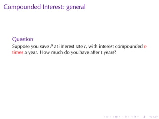
- 52. Compounded Interest: general Question Suppose you save P at interest rate r, with interest compounded n times a year. How much do you have after t years? . . . . . .
- 53. Compounded Interest: general Question Suppose you save P at interest rate r, with interest compounded n times a year. How much do you have after t years? Answer ( r )nt B(t) = P 1 + n . . . . . .
- 54. Compounded Interest: continuous Question Suppose you save P at interest rate r, with interest compounded every instant. How much do you have after t years? . . . . . .
- 55. Compounded Interest: continuous Question Suppose you save P at interest rate r, with interest compounded every instant. How much do you have after t years? Answer ( ( ) r )nt 1 rnt B(t) = lim P 1 + = lim P 1 + n→∞ n n→∞ n [ ( )n ]rt 1 = P lim 1 + n→∞ n independent of P, r, or t . . . . . .
- 56. The magic number Definition ( )n 1 e = lim 1+ n→∞ n . . . . . .
- 57. The magic number Definition ( )n 1 e = lim 1+ n→∞ n So now continuously-compounded interest can be expressed as B(t) = Pert . . . . . . .
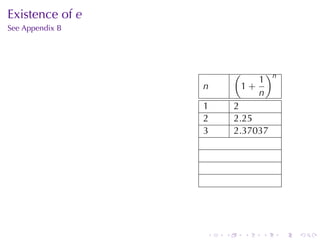
- 58. Existence of e See Appendix B ( )n 1 n 1+ n 1 2 2 2.25 . . . . . .
- 59. Existence of e See Appendix B ( )n 1 n 1+ n 1 2 2 2.25 3 2.37037 . . . . . .
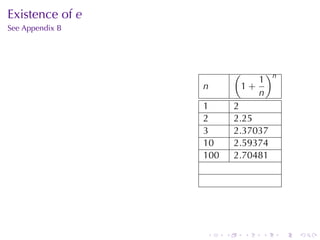
- 60. Existence of e See Appendix B ( )n 1 n 1+ n 1 2 2 2.25 3 2.37037 10 2.59374 . . . . . .
- 61. Existence of e See Appendix B ( )n 1 n 1+ n 1 2 2 2.25 3 2.37037 10 2.59374 100 2.70481 . . . . . .
- 62. Existence of e See Appendix B ( )n 1 n 1+ n 1 2 2 2.25 3 2.37037 10 2.59374 100 2.70481 1000 2.71692 . . . . . .
- 63. Existence of e See Appendix B ( )n 1 n 1+ n 1 2 2 2.25 3 2.37037 10 2.59374 100 2.70481 1000 2.71692 106 2.71828 . . . . . .
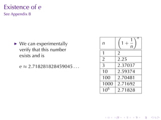
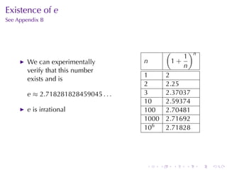
- 64. Existence of e See Appendix B ( )n 1 We can experimentally n 1+ n verify that this number 1 2 exists and is 2 2.25 e ≈ 2.718281828459045 . . . 3 2.37037 10 2.59374 100 2.70481 1000 2.71692 106 2.71828 . . . . . .
- 65. Existence of e See Appendix B ( )n 1 We can experimentally n 1+ n verify that this number 1 2 exists and is 2 2.25 e ≈ 2.718281828459045 . . . 3 2.37037 10 2.59374 e is irrational 100 2.70481 1000 2.71692 106 2.71828 . . . . . .
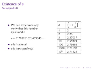
- 66. Existence of e See Appendix B ( )n 1 We can experimentally n 1+ n verify that this number 1 2 exists and is 2 2.25 e ≈ 2.718281828459045 . . . 3 2.37037 10 2.59374 e is irrational 100 2.70481 e is transcendental 1000 2.71692 106 2.71828 . . . . . .
- 67. Meet the Mathematician: Leonhard Euler Born in Switzerland, lived in Prussia (Germany) and Russia Eyesight trouble all his life, blind from 1766 onward Hundreds of contributions to calculus, number theory, graph theory, fluid mechanics, optics, and astronomy Leonhard Paul Euler Swiss, 1707–1783 . . . . . .
- 68. A limit Question eh − 1 What is lim ? h→0 h . . . . . .
- 69. A limit Question eh − 1 What is lim ? h→0 h Answer If h is small enough, e ≈ (1 + h)1/h . So eh − 1 ≈1 h . . . . . .
- 70. A limit Question eh − 1 What is lim ? h→0 h Answer If h is small enough, e ≈ (1 + h)1/h . So eh − 1 ≈1 h eh − 1 In fact, lim = 1. h→0 h This can be used to characterize e: 2h − 1 3h − 1 lim = 0.693 · · · < 1 and lim = 1.099 · · · < 1 h→0 h h→0 h . . . . . .