Lesson 13: Exponential and Logarithmic Functions (slides)
6 likes3,974 views

The document provides an outline and definitions for sections 3.1 and 3.2 of a calculus class, which cover exponential and logarithmic functions. It defines exponential functions, establishes conventions for exponents of all types, and graphs exponential functions. Key points covered include the properties of exponential functions and defining exponents for non-whole number bases.


![Compounded Interest: continuous
Ques on
Suppose you save P at interest rate r, with interest compounded
every instant. How much do you have a er t years?
Answer
( ( )rnt
r )nt 1
B(t) = lim P 1 + = lim P 1 +
n→∞ n n→∞ n
[ ( )n ]rt
1
= P lim 1 +
n→∞ n
independent of P, r, or t](https://image.slidesharecdn.com/lesson13-exponentialfunctions001slides-110315100550-phpapp02/85/Lesson-13-Exponential-and-Logarithmic-Functions-slides-69-320.jpg)


![A limit
Ques on
eh − 1
What is lim ?
h→0 h
Answer
e = lim (1 + 1/n)n = lim (1 + h)1/h . So for a small h,
n→∞ h→0
e ≈ (1 + h) 1/h
. So
[ ]h
eh − 1 (1 + h)1/h − 1
≈ =1
h h](https://image.slidesharecdn.com/lesson13-exponentialfunctions001slides-110315100550-phpapp02/85/Lesson-13-Exponential-and-Logarithmic-Functions-slides-83-320.jpg)


Lesson 13: Exponential and Logarithmic Functions (slides)
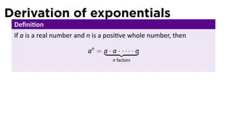
- 1. Sec on 3.1–3.2 Exponen al and Logarithmic Func ons V63.0121.001: Calculus I Professor Ma hew Leingang New York University March 9, 2011 .
- 2. Announcements Midterm is graded. average = 44, median=46, SD =10 There is WebAssign due a er Spring Break. Quiz 3 on 2.6, 2.8, 3.1, 3.2 on March 30
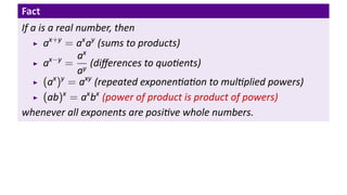
- 3. Midterm Statistics Average: 43.86/60 = 73.1% Median: 46/60 = 76.67% Standard Devia on: 10.64% “good” is anything above average and “great” is anything more than one standard devia on above average. More than one SD below the mean is cause for concern.
- 4. Objectives for Sections 3.1 and 3.2 Know the defini on of an exponen al func on Know the proper es of exponen al func ons Understand and apply the laws of logarithms, including the change of base formula.
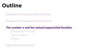
- 5. Outline Defini on of exponen al func ons Proper es of exponen al Func ons The number e and the natural exponen al func on Compound Interest The number e A limit Logarithmic Func ons
- 6. Derivation of exponentials Defini on If a is a real number and n is a posi ve whole number, then an = a · a · · · · · a n factors
- 7. Derivation of exponentials Defini on If a is a real number and n is a posi ve whole number, then an = a · a · · · · · a n factors Examples 23 = 2 · 2 · 2 = 8 34 = 3 · 3 · 3 · 3 = 81 (−1)5 = (−1)(−1)(−1)(−1)(−1) = −1
- 8. Anatomy of a power Defini on A power is an expression of the form ab . The number a is called the base. The number b is called the exponent.
- 9. Fact If a is a real number, then ax+y = ax ay (sums to products) x−y ax a = y a (ax )y = axy (ab)x = ax bx whenever all exponents are posi ve whole numbers.
- 10. Fact If a is a real number, then ax+y = ax ay (sums to products) x−y ax a = y (differences to quo ents) a (ax )y = axy (ab)x = ax bx whenever all exponents are posi ve whole numbers.
- 11. Fact If a is a real number, then ax+y = ax ay (sums to products) x−y ax a = y (differences to quo ents) a (ax )y = axy (repeated exponen a on to mul plied powers) (ab)x = ax bx whenever all exponents are posi ve whole numbers.
- 12. Fact If a is a real number, then ax+y = ax ay (sums to products) x−y ax a = y (differences to quo ents) a (ax )y = axy (repeated exponen a on to mul plied powers) (ab)x = ax bx (power of product is product of powers) whenever all exponents are posi ve whole numbers.
- 13. Fact If a is a real number, then ax+y = ax ay (sums to products) x−y ax a = y (differences to quo ents) a (ax )y = axy (repeated exponen a on to mul plied powers) (ab)x = ax bx (power of product is product of powers) whenever all exponents are posi ve whole numbers.
- 14. Fact If a is a real number, then ax+y = ax ay (sums to products) x−y ax a = y (differences to quo ents) a (ax )y = axy (repeated exponen a on to mul plied powers) (ab)x = ax bx (power of product is product of powers) whenever all exponents are posi ve whole numbers. Proof. Check for yourself: ax+y = a · a · · · · · a = a · a · · · · · a · a · a · · · · · a = ax ay x + y factors x factors y factors
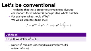
- 15. Let’s be conventional The desire that these proper es remain true gives us conven ons for ax when x is not a posi ve whole number.
- 16. Let’s be conventional The desire that these proper es remain true gives us conven ons for ax when x is not a posi ve whole number. For example, what should a0 be? We would want this to be true: ! an = an+0 = an · a0
- 17. Let’s be conventional The desire that these proper es remain true gives us conven ons for ax when x is not a posi ve whole number. For example, what should a0 be? We would want this to be true: n ! ! a an = an+0 = an · a0 =⇒ a0 = n = 1 a
- 18. Let’s be conventional The desire that these proper es remain true gives us conven ons for ax when x is not a posi ve whole number. For example, what should a0 be? We would want this to be true: n ! ! a an = an+0 = an · a0 =⇒ a0 = n = 1 a Defini on If a ̸= 0, we define a0 = 1.
- 19. Let’s be conventional The desire that these proper es remain true gives us conven ons for ax when x is not a posi ve whole number. For example, what should a0 be? We would want this to be true: n ! ! a an = an+0 = an · a0 =⇒ a0 = n = 1 a Defini on If a ̸= 0, we define a0 = 1. No ce 00 remains undefined (as a limit form, it’s indeterminate).
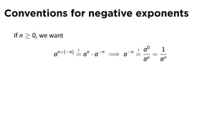
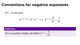
- 20. Conventions for negative exponents If n ≥ 0, we want an+(−n) = an · a−n !
- 21. Conventions for negative exponents If n ≥ 0, we want a0 1 an+(−n) = an · a−n =⇒ a−n = ! ! = n an a
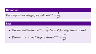
- 22. Conventions for negative exponents If n ≥ 0, we want a0 1 an+(−n) = an · a−n =⇒ a−n = ! ! = n an a Defini on 1 If n is a posi ve integer, we define a−n = . an
- 23. Defini on 1 If n is a posi ve integer, we define a−n = . an
- 24. Defini on 1 If n is a posi ve integer, we define a−n = . an Fact 1 The conven on that a−n = “works” for nega ve n as well. an m−n am If m and n are any integers, then a = n. a
- 25. Conventions for fractional exponents If q is a posi ve integer, we want ! (a1/q )q = a1 = a
- 26. Conventions for fractional exponents If q is a posi ve integer, we want ! ! √ (a1/q )q = a1 = a =⇒ a1/q = q a
- 27. Conventions for fractional exponents If q is a posi ve integer, we want ! ! √ (a1/q )q = a1 = a =⇒ a1/q = q a Defini on √ If q is a posi ve integer, we define a1/q = q a. We must have a ≥ 0 if q is even.
- 28. Conventions for fractional exponents If q is a posi ve integer, we want ! ! √ (a1/q )q = a1 = a =⇒ a1/q = q a Defini on √ If q is a posi ve integer, we define a1/q = q a. We must have a ≥ 0 if q is even. √q (√ )p No ce that ap = q a . So we can unambiguously say ap/q = (ap )1/q = (a1/q )p
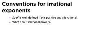
- 29. Conventions for irrational exponents So ax is well-defined if a is posi ve and x is ra onal. What about irra onal powers?
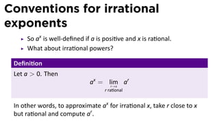
- 30. Conventions for irrational exponents So ax is well-defined if a is posi ve and x is ra onal. What about irra onal powers? Defini on Let a > 0. Then ax = lim ar r→x r ra onal
- 31. Conventions for irrational exponents So ax is well-defined if a is posi ve and x is ra onal. What about irra onal powers? Defini on Let a > 0. Then ax = lim ar r→x r ra onal In other words, to approximate ax for irra onal x, take r close to x but ra onal and compute ar .
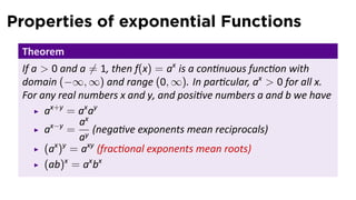
- 32. Approximating a power with an irrational exponent r 2r 3 23 √=8 10 3.1 231/10 = √ 31 ≈ 8.57419 2 100 3.14 2314/100 = √ 314 ≈ 8.81524 2 1000 3.141 23141/1000 = 23141 ≈ 8.82135 The limit (numerically approximated is) 2π ≈ 8.82498
- 33. Graphs of exponential functions y . x
- 34. Graphs of exponential functions y y = 1x . x
- 35. Graphs of exponential functions y y = 2x y = 1x . x
- 36. Graphs of exponential functions y y = 3x = 2x y y = 1x . x
- 37. Graphs of exponential functions y y = 10x 3x = 2x y= y y = 1x . x
- 38. Graphs of exponential functions y y = 10x 3x = 2x y= y y = 1.5x y = 1x . x
- 39. Graphs of exponential functions y y = (1/2)x y = 10x 3x = 2x y= y y = 1.5x y = 1x . x
- 40. Graphs of exponential functions y y = (y/= x(1/3)x 1 2) y = 10x 3x = 2x y= y y = 1.5x y = 1x . x
- 41. Graphs of exponential functions y y = (y/= x(1/3)x 1 2) y = (1/10y x= 10x 3x = 2x ) y= y y = 1.5x y = 1x . x
- 42. Graphs of exponential functions y y y =y/=3(1/3)x = (1(2/x)x 2) y = (1/10y x= 10x 3x = 2x ) y= y y = 1.5x y = 1x . x
- 43. Outline Defini on of exponen al func ons Proper es of exponen al Func ons The number e and the natural exponen al func on Compound Interest The number e A limit Logarithmic Func ons
- 44. Properties of exponential Functions Theorem If a > 0 and a ̸= 1, then f(x) = ax is a con nuous func on with domain (−∞, ∞) and range (0, ∞). In par cular, ax > 0 for all x. For any real numbers x and y, and posi ve numbers a and b we have ax+y = ax ay x−y ax a = y a (a ) = axy x y (ab)x = ax bx
- 45. Properties of exponential Functions Theorem If a > 0 and a ̸= 1, then f(x) = ax is a con nuous func on with domain (−∞, ∞) and range (0, ∞). In par cular, ax > 0 for all x. For any real numbers x and y, and posi ve numbers a and b we have ax+y = ax ay x−y ax a = y (nega ve exponents mean reciprocals) a (a ) = axy x y (ab)x = ax bx
- 46. Properties of exponential Functions Theorem If a > 0 and a ̸= 1, then f(x) = ax is a con nuous func on with domain (−∞, ∞) and range (0, ∞). In par cular, ax > 0 for all x. For any real numbers x and y, and posi ve numbers a and b we have ax+y = ax ay x−y ax a = y (nega ve exponents mean reciprocals) a (a ) = axy (frac onal exponents mean roots) x y (ab)x = ax bx
- 47. Proof. This is true for posi ve integer exponents by natural defini on Our conven onal defini ons make these true for ra onal exponents Our limit defini on make these for irra onal exponents, too
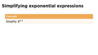
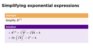
- 48. Simplifying exponential expressions Example Simplify: 82/3
- 49. Simplifying exponential expressions Example Simplify: 82/3 Solu on √ 3 √ 2/3 = 82 = 64 = 4 3 8
- 50. Simplifying exponential expressions Example Simplify: 82/3 Solu on √3 √ 2/3 8 = 82 = 64 = 4 3 (√ )2 8 = 22 = 4. 3 Or,
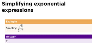
- 51. Simplifying exponential expressions Example √ 8 Simplify: 21/2
- 52. Simplifying exponential expressions Example √ 8 Simplify: 21/2 Answer 2
- 53. Limits of exponential functions Fact (Limits of exponen al func ons) y y (1 y )/3 x y = =/(1= )(2/3)x y = y1/1010= 2x = 1.5 2 x ( = =x 3x y y ) x y If a > 1, then lim ax = ∞ and x→∞ lim ax = 0 x→−∞ If 0 < a < 1, then y = 1x lim ax = 0 and . x x→∞ lim ax = ∞ x→−∞
- 54. Outline Defini on of exponen al func ons Proper es of exponen al Func ons The number e and the natural exponen al func on Compound Interest The number e A limit Logarithmic Func ons
- 55. Compounded Interest Ques on Suppose you save $100 at 10% annual interest, with interest compounded once a year. How much do you have A er one year? A er two years? A er t years?
- 56. Compounded Interest Ques on Suppose you save $100 at 10% annual interest, with interest compounded once a year. How much do you have A er one year? A er two years? A er t years? Answer $100 + 10% = $110
- 57. Compounded Interest Ques on Suppose you save $100 at 10% annual interest, with interest compounded once a year. How much do you have A er one year? A er two years? A er t years? Answer $100 + 10% = $110 $110 + 10% = $110 + $11 = $121
- 58. Compounded Interest Ques on Suppose you save $100 at 10% annual interest, with interest compounded once a year. How much do you have A er one year? A er two years? A er t years? Answer $100 + 10% = $110 $110 + 10% = $110 + $11 = $121 $100(1.1)t .
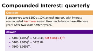
- 59. Compounded Interest: quarterly Ques on Suppose you save $100 at 10% annual interest, with interest compounded four mes a year. How much do you have A er one year? A er two years? A er t years?
- 60. Compounded Interest: quarterly Ques on Suppose you save $100 at 10% annual interest, with interest compounded four mes a year. How much do you have A er one year? A er two years? A er t years? Answer $100(1.025)4 = $110.38,
- 61. Compounded Interest: quarterly Ques on Suppose you save $100 at 10% annual interest, with interest compounded four mes a year. How much do you have A er one year? A er two years? A er t years? Answer $100(1.025)4 = $110.38, not $100(1.1)4 !
- 62. Compounded Interest: quarterly Ques on Suppose you save $100 at 10% annual interest, with interest compounded four mes a year. How much do you have A er one year? A er two years? A er t years? Answer $100(1.025)4 = $110.38, not $100(1.1)4 ! $100(1.025)8 = $121.84
- 63. Compounded Interest: quarterly Ques on Suppose you save $100 at 10% annual interest, with interest compounded four mes a year. How much do you have A er one year? A er two years? A er t years? Answer $100(1.025)4 = $110.38, not $100(1.1)4 ! $100(1.025)8 = $121.84 $100(1.025)4t .
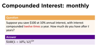
- 64. Compounded Interest: monthly Ques on Suppose you save $100 at 10% annual interest, with interest compounded twelve mes a year. How much do you have a er t years?
- 65. Compounded Interest: monthly Ques on Suppose you save $100 at 10% annual interest, with interest compounded twelve mes a year. How much do you have a er t years? Answer $100(1 + 10%/12)12t
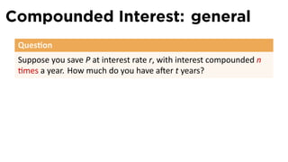
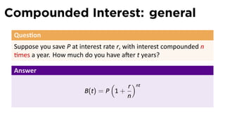
- 66. Compounded Interest: general Ques on Suppose you save P at interest rate r, with interest compounded n mes a year. How much do you have a er t years?
- 67. Compounded Interest: general Ques on Suppose you save P at interest rate r, with interest compounded n mes a year. How much do you have a er t years? Answer ( r )nt B(t) = P 1 + n
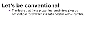
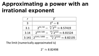
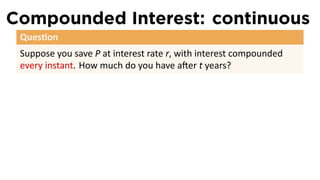
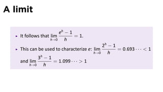
- 68. Compounded Interest: continuous Ques on Suppose you save P at interest rate r, with interest compounded every instant. How much do you have a er t years?
- 69. Compounded Interest: continuous Ques on Suppose you save P at interest rate r, with interest compounded every instant. How much do you have a er t years? Answer ( ( )rnt r )nt 1 B(t) = lim P 1 + = lim P 1 + n→∞ n n→∞ n [ ( )n ]rt 1 = P lim 1 + n→∞ n independent of P, r, or t
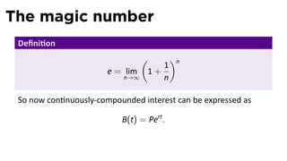
- 70. The magic number Defini on ( )n 1 e = lim 1 + n→∞ n
- 71. The magic number Defini on ( )n 1 e = lim 1 + n→∞ n So now con nuously-compounded interest can be expressed as B(t) = Pert .
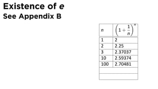
- 72. Existence of e See Appendix B ( )n 1 n 1+ n 1 2 2 2.25
- 73. Existence of e See Appendix B ( )n 1 n 1+ n 1 2 2 2.25 3 2.37037
- 74. Existence of e See Appendix B ( )n 1 n 1+ n 1 2 2 2.25 3 2.37037 10 2.59374
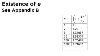
- 75. Existence of e See Appendix B ( )n 1 n 1+ n 1 2 2 2.25 3 2.37037 10 2.59374 100 2.70481
- 76. Existence of e See Appendix B ( )n 1 n 1+ n 1 2 2 2.25 3 2.37037 10 2.59374 100 2.70481 1000 2.71692
- 77. Existence of e See Appendix B ( )n 1 n 1+ n 1 2 2 2.25 3 2.37037 10 2.59374 100 2.70481 1000 2.71692 106 2.71828
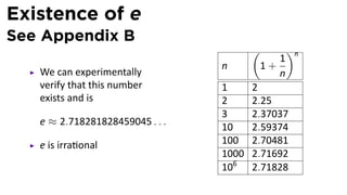
- 78. Existence of e See Appendix B ( )n 1 n 1+ We can experimentally n verify that this number 1 2 exists and is 2 2.25 3 2.37037 e ≈ 2.718281828459045 . . . 10 2.59374 100 2.70481 1000 2.71692 106 2.71828
- 79. Existence of e See Appendix B ( )n 1 n 1+ We can experimentally n verify that this number 1 2 exists and is 2 2.25 3 2.37037 e ≈ 2.718281828459045 . . . 10 2.59374 e is irra onal 100 2.70481 1000 2.71692 106 2.71828
- 80. Existence of e See Appendix B ( )n 1 n 1+ We can experimentally n verify that this number 1 2 exists and is 2 2.25 3 2.37037 e ≈ 2.718281828459045 . . . 10 2.59374 e is irra onal 100 2.70481 1000 2.71692 e is transcendental 106 2.71828
- 81. Meet the Mathematician: Leonhard Euler Born in Switzerland, lived in Prussia (Germany) and Russia Eyesight trouble all his life, blind from 1766 onward Hundreds of contribu ons to calculus, number theory, graph theory, fluid mechanics, Leonhard Paul Euler op cs, and astronomy Swiss, 1707–1783
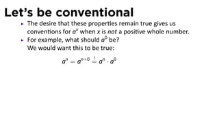
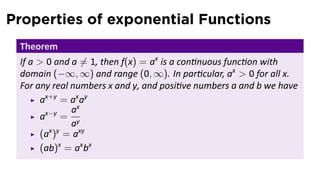
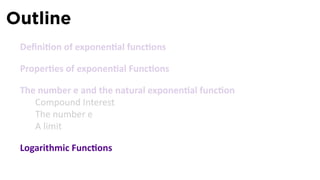
- 82. A limit Ques on eh − 1 What is lim ? h→0 h
- 83. A limit Ques on eh − 1 What is lim ? h→0 h Answer e = lim (1 + 1/n)n = lim (1 + h)1/h . So for a small h, n→∞ h→0 e ≈ (1 + h) 1/h . So [ ]h eh − 1 (1 + h)1/h − 1 ≈ =1 h h
- 84. A limit eh − 1 It follows that lim = 1. h→0 h 2h − 1 This can be used to characterize e: lim = 0.693 · · · < 1 h→0 h 3h − 1 and lim = 1.099 · · · > 1 h→0 h
- 85. Outline Defini on of exponen al func ons Proper es of exponen al Func ons The number e and the natural exponen al func on Compound Interest The number e A limit Logarithmic Func ons
- 86. Logarithms Defini on The base a logarithm loga x is the inverse of the func on ax y = loga x ⇐⇒ x = ay The natural logarithm ln x is the inverse of ex . So y = ln x ⇐⇒ x = ey .
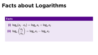
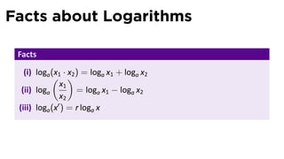
- 87. Facts about Logarithms Facts (i) loga (x1 · x2 ) = loga x1 + loga x2
- 88. Facts about Logarithms Facts (i) loga (x1 · x2 ) = loga x1 + loga x2 ( ) x1 (ii) loga = loga x1 − loga x2 x2
- 89. Facts about Logarithms Facts (i) loga (x1 · x2 ) = loga x1 + loga x2 ( ) x1 (ii) loga = loga x1 − loga x2 x2 (iii) loga (xr ) = r loga x
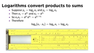
- 90. Logarithms convert products to sums Suppose y1 = loga x1 and y2 = loga x2 Then x1 = ay1 and x2 = ay2 So x1 x2 = ay1 ay2 = ay1 +y2 Therefore loga (x1 · x2 ) = loga x1 + loga x2
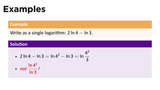
- 91. Examples Example Write as a single logarithm: 2 ln 4 − ln 3.
- 92. Examples Example Write as a single logarithm: 2 ln 4 − ln 3. Solu on 42 2 ln 4 − ln 3 = ln 42 − ln 3 = ln 3 ln 42 not ! ln 3
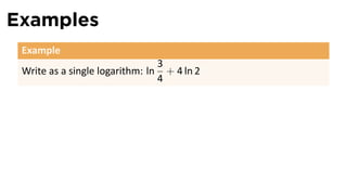
- 93. Examples Example 3 Write as a single logarithm: ln + 4 ln 2 4
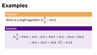
- 94. Examples Example 3 Write as a single logarithm: ln + 4 ln 2 4 Solu on 3 ln + 4 ln 2 = ln 3 − ln 4 + 4 ln 2 = ln 3 − 2 ln 2 + 4 ln 2 4 = ln 3 + 2 ln 2 = ln(3 · 22 ) = ln 12
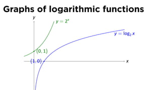
- 95. Graphs of logarithmic functions y y = 2x y = log2 x (0, 1) . (1, 0) x
- 96. Graphs of logarithmic functions y y =y3= 2x x y = log2 x y = log3 x (0, 1) . (1, 0) x
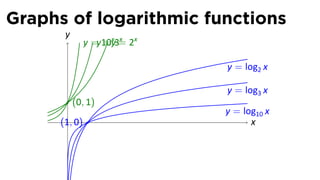
- 97. Graphs of logarithmic functions y y =y10y3= 2x =x x y = log2 x y = log3 x (0, 1) y = log10 x . (1, 0) x
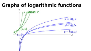
- 98. Graphs of logarithmic functions y y =x ex y =y10y3= 2x = x y = log2 x yy= log3 x = ln x (0, 1) y = log10 x . (1, 0) x
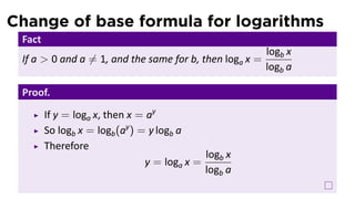
- 99. Change of base formula for logarithms Fact logb x If a > 0 and a ̸= 1, and the same for b, then loga x = logb a
- 100. Change of base formula for logarithms Fact logb x If a > 0 and a ̸= 1, and the same for b, then loga x = logb a Proof. If y = loga x, then x = ay So logb x = logb (ay ) = y logb a Therefore logb x y = loga x = logb a
- 101. Example of changing base Example Find log2 8 by using log10 only.
- 102. Example of changing base Example Find log2 8 by using log10 only. Solu on log10 8 0.90309 log2 8 = ≈ =3 log10 2 0.30103
- 103. Example of changing base Example Find log2 8 by using log10 only. Solu on log10 8 0.90309 log2 8 = ≈ =3 log10 2 0.30103 Surprised?
- 104. Example of changing base Example Find log2 8 by using log10 only. Solu on log10 8 0.90309 log2 8 = ≈ =3 log10 2 0.30103 Surprised? No, log2 8 = log2 23 = 3 directly.
- 105. Upshot of changing base The point of the change of base formula logb x 1 loga x = = · logb x = constant · logb x logb a logb a is that all the logarithmic func ons are mul ples of each other. So just pick one and call it your favorite. Engineers like the common logarithm log = log10 Computer scien sts like the binary logarithm lg = log2 Mathema cians like natural logarithm ln = loge Naturally, we will follow the mathema cians. Just don’t pronounce it “lawn.”
- 106. “lawn” . . Image credit: Selva
- 107. Summary Exponen als turn sums into products Logarithms turn products into sums Slide rule scabbards are wicked cool