![Dynamic Time Wrapping (DTW)
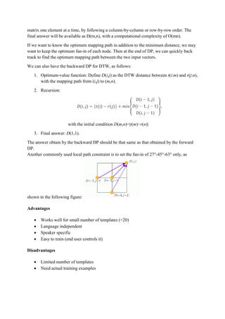
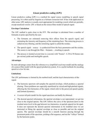
Dynamic time wrapping (DTW) is a well-known technique to find an optimal alignment
between two given (time-dependent) sequences under certain restrictions (Fig. 01). Intuitively,
the sequences are warped in a nonlinear fashion to match each other. Originally, DTW has been
used to compare different speech patterns in automatic speech recognition. In fields such as
data mining and information retrieval, DTW has been successfully applied to automatically
cope with time deformations and different speeds associated with time-dependent data. Fig-
01 showing two speech signal aligned with DTW.
Fig-01: Two Speech Signal Aligned using DTW
Fig. 02: Time alignment of two time-dependent sequences. Aligned points are indicated by
the arrows
The distance between two point, x=[x1,x2,...,xn] and y=[y1,y2,...,yn]
in a n-dimensional space can be computed via the Euclidean distance:
dist(x,y)=∥x−y∥=√((𝑥1 − 𝑦1)2 + (𝑥2 − 𝑦2)2 + ⋯ + (𝑥 𝑛 − 𝑦 𝑛)2)](https://image.slidesharecdn.com/dynamictimewrappingdtwvectorquantizationvqlinearpredictivecodinglpc-170925192730/85/Dynamic-time-wrapping-dtw-vector-quantization-vq-linear-predictive-coding-lpc-1-320.jpg)

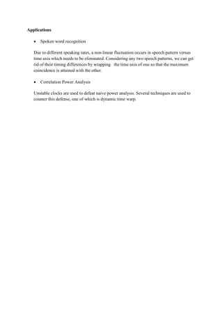
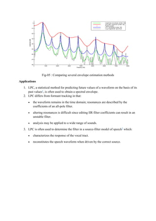
![An example of two dimensional vector quantizer is shown in Fig-03. The two dimensional
region shown in Fig-03 is called as the voronoi region, which in turn contains several numbers
of small hexagonal regions. The hexagonal regions defined by the red borders are called as the
encoding regions. The green dots represent the vectors to be quantized which fall in different
hexagonal regions and the blue circles represent the codeword‟s (centroids). The vectors (green
dots) falling in a particular hexagonal region is best represented by the codeword (blue circle)
falling in that hexagonal region.
Vector quantization technique has become a great tool with the development of non variational
design algorithms like the Linde, Buzo, Gray (LBG) algorithm. On the other hand besides
spectral distortion the vector quantizer is having its own limitations like the computational
complexity and memory requirements required for the searching and storing of the codebooks.
For applications requiring higher bit-rates the computational complexity and memory
requirements increases exponentially. The block diagram of a vector quantizer is shown in Fig-
04
Fig-04 : Block diagram of Vector Quantizer
Let 𝑠 𝑘 = [𝑠1, 𝑠2, … . 𝑠 𝑁] 𝑇
be an N dimensional vector with real valued samples in the range 1≤
k ≤N. The superscript T in the vector 𝑠 𝑘 denotes the transpose of the vector. In vector
quantization, a real valued N dimensional input vector 𝑠 𝑘 is matched with the real valued N
dimensional codewords of the codebook N = 2 𝑏
. The code word that best matches the input
vector with lowest distortion is taken and the input vector is replaced by it. The codebook
consists of a finite set of codewords C = 𝐶𝑖 , 1≤ i ≤L, where 𝐶𝑖 =
[𝐶1𝑖, 𝐶2𝑖, … . 𝐶 𝑁𝑖] 𝑇
, where C is the codebook, L is the length of the codebook and 𝐶𝑖 denote
the ith codeword in a codebook.
Advantages
Advantages with vector quantization compared to scalar quantization.
Can utilize the memory of the source.
The distortion at a given rate will always be lower when increasing the number of
dimensions, even for a memoryless source.
Index iInput Vector
Buffe r
Codebook with
Codeword’s
C
Vector
Quantizer
( )ns ks
iC](https://image.slidesharecdn.com/dynamictimewrappingdtwvectorquantizationvqlinearpredictivecodinglpc-170925192730/85/Dynamic-time-wrapping-dtw-vector-quantization-vq-linear-predictive-coding-lpc-6-320.jpg)
Dynamic time wrapping (dtw), vector quantization(vq), linear predictive coding (lpc)
- 1. Dynamic Time Wrapping (DTW) Dynamic time wrapping (DTW) is a well-known technique to find an optimal alignment between two given (time-dependent) sequences under certain restrictions (Fig. 01). Intuitively, the sequences are warped in a nonlinear fashion to match each other. Originally, DTW has been used to compare different speech patterns in automatic speech recognition. In fields such as data mining and information retrieval, DTW has been successfully applied to automatically cope with time deformations and different speeds associated with time-dependent data. Fig- 01 showing two speech signal aligned with DTW. Fig-01: Two Speech Signal Aligned using DTW Fig. 02: Time alignment of two time-dependent sequences. Aligned points are indicated by the arrows The distance between two point, x=[x1,x2,...,xn] and y=[y1,y2,...,yn] in a n-dimensional space can be computed via the Euclidean distance: dist(x,y)=∥x−y∥=√((𝑥1 − 𝑦1)2 + (𝑥2 − 𝑦2)2 + ⋯ + (𝑥 𝑛 − 𝑦 𝑛)2)
- 2. However, if the length of x is different from y, then we cannot use the above formula to compute the distance. Instead, we need a more flexible method that can find the best mapping from elements in x to those in y in order to compute the distance. The goal of dynamic time wrapping (DTW for short) is to find the best mapping with the minimum distance by the use of DP. The method is called "time wrapping " since both x and y are usually vectors of time series and we need to compress or expand in time in order to find the best mapping. We shall give the formula for DTW in this section. Let t and r be two vectors of lengths m and n, respectively. The goal of DTW is to find a mapping path {(p1,q1),(p2,q2),...,(pk,qk)} such that the distance on this mapping path ∑ |𝑡(𝑝𝑖) − 𝑟(𝑞𝑖)|𝑘 𝑖=0 is minimized, with the following constraints: Boundary conditions: (p1,q1)=(1,1), (pk,qk)=(m,n). This is a typical example of "anchored beginning" and "anchored end". Local constraint: For any given node (i,j) in the path, the possible fan-in nodes are restricted to (i−1,j), (i,j−1), (i−1,j−1). This local constraint guarantees that the mapping path is monotonically non-decreasing in its first and second arguments. Moreover, for any given element in t, we should be able to find at least one corresponding element in r, and vice versa. How can we find the optimum mapping path in DTW? An obvious choice is forward DP, which can be summarized in the following three steps: 1. Optimum-value function: Define D(i,j) as the DTW distance between t(1:i) and r(1:j), with the mapping path starting from (1,1) to (i,j). 2. Recursion: with the initial condition D(1,1)=|t(1)−r(1)| 3. Final answer: D(m,n). In practice, we need to construct a matrix D of dimensions m×n first and fill in the value of D(1,1) by using the initial condition. Then by using the recursive formula, we fill the whole
- 3. matrix one element at a time, by following a column-by-column or row-by-row order. The final answer will be available as D(m,n), with a computational complexity of O(mn). If we want to know the optimum mapping path in addition to the minimum distance, we may want to keep the optimum fan-in of each node. Then at the end of DP, we can quickly back track to find the optimum mapping path between the two input vectors. We can also have the backward DP for DTW, as follows: 1. Optimum-value function: Define D(i,j) as the DTW distance between t(i:m) and r(j:n), with the mapping path from (i,j) to (m,n). 2. Recursion: with the initial condition D(m,n)=|t(m)−r(n)| 3. Final answer: D(1,1). The answer obtain by the backward DP should be that same as that obtained by the forward DP. Another commonly used local path constraint is to set the fan-in of 27°-45°-63° only, as shown in the following figure: Advantages Works well for small number of templates (<20) Language independent Speaker specific Easy to train (end user controls it) Disadvantages Limited number of templates Need actual training examples
- 4. Applications Spoken word recognition Due to different speaking rates, a non-linear fluctuation occurs in speech pattern versus time axis which needs to be eliminated. Considering any two speech patterns, we can get rid of their timing differences by wrapping the time axis of one so that the maximum coincidence is attained with the other. Correlation Power Analysis Unstable clocks are used to defeat naive power analysis. Several techniques are used to counter this defense, one of which is dynamic time warp.
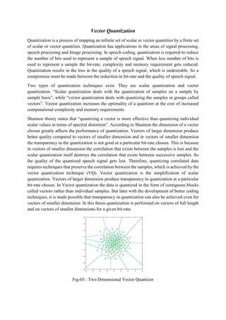
- 5. Vector Quantization Quantization is a process of mapping an infinite set of scalar or vector quantities by a finite set of scalar or vector quantities. Quantization has applications in the areas of signal processing, speech processing and Image processing. In speech coding, quantization is required to reduce the number of bits used to represent a sample of speech signal. When less number of bits is used to represent a sample the bit-rate, complexity and memory requirement gets reduced. Quantization results in the loss in the quality of a speech signal, which is undesirable. So a compromise must be made between the reduction in bit-rate and the quality of speech signal. Two types of quantization techniques exist. They are scalar quantization and vector quantization. “Scalar quantization deals with the quantization of samples on a sample by sample basis”, while “vector quantization deals with quantizing the samples in groups called vectors”. Vector quantization increases the optimality of a quantizer at the cost of increased computational complexity and memory requirements. Shannon theory states that “quantizing a vector is more effective than quantizing individual scalar values in terms of spectral distortion”. According to Shannon the dimension of a vector chosen greatly affects the performance of quantization. Vectors of larger dimension produce better quality compared to vectors of smaller dimension and in vectors of smaller dimension the transparency in the quantization is not good at a particular bit-rate chosen. This is because in vectors of smaller dimension the correlation that exists between the samples is lost and the scalar quantization itself destroys the correlation that exists between successive samples. So the quality of the quantized speech signal gets lost. Therefore, quantizing correlated data requires techniques that preserve the correlation between the samples, which is achieved by the vector quantization technique (VQ). Vector quantization is the simplification of scalar quantization. Vectors of larger dimension produce transparency in quantization at a particular bit-rate chosen. In Vector quantization the data is quantized in the form of contiguous blocks called vectors rather than individual samples. But later with the development of better coding techniques, it is made possible that transparency in quantization can also be achieved even for vectors of smaller dimension. In this thesis quantization is performed on vectors of full length and on vectors of smaller dimensions for a given bit-rate. Fig-03 : Two Dimensional Vector Quantizer
- 6. An example of two dimensional vector quantizer is shown in Fig-03. The two dimensional region shown in Fig-03 is called as the voronoi region, which in turn contains several numbers of small hexagonal regions. The hexagonal regions defined by the red borders are called as the encoding regions. The green dots represent the vectors to be quantized which fall in different hexagonal regions and the blue circles represent the codeword‟s (centroids). The vectors (green dots) falling in a particular hexagonal region is best represented by the codeword (blue circle) falling in that hexagonal region. Vector quantization technique has become a great tool with the development of non variational design algorithms like the Linde, Buzo, Gray (LBG) algorithm. On the other hand besides spectral distortion the vector quantizer is having its own limitations like the computational complexity and memory requirements required for the searching and storing of the codebooks. For applications requiring higher bit-rates the computational complexity and memory requirements increases exponentially. The block diagram of a vector quantizer is shown in Fig- 04 Fig-04 : Block diagram of Vector Quantizer Let 𝑠 𝑘 = [𝑠1, 𝑠2, … . 𝑠 𝑁] 𝑇 be an N dimensional vector with real valued samples in the range 1≤ k ≤N. The superscript T in the vector 𝑠 𝑘 denotes the transpose of the vector. In vector quantization, a real valued N dimensional input vector 𝑠 𝑘 is matched with the real valued N dimensional codewords of the codebook N = 2 𝑏 . The code word that best matches the input vector with lowest distortion is taken and the input vector is replaced by it. The codebook consists of a finite set of codewords C = 𝐶𝑖 , 1≤ i ≤L, where 𝐶𝑖 = [𝐶1𝑖, 𝐶2𝑖, … . 𝐶 𝑁𝑖] 𝑇 , where C is the codebook, L is the length of the codebook and 𝐶𝑖 denote the ith codeword in a codebook. Advantages Advantages with vector quantization compared to scalar quantization. Can utilize the memory of the source. The distortion at a given rate will always be lower when increasing the number of dimensions, even for a memoryless source. Index iInput Vector Buffe r Codebook with Codeword’s C Vector Quantizer ( )ns ks iC
- 7. Disadvantages Disadvantages with vector quantization compared to scalar quantization. Both the storage space and the time needed to perform the quantization grows faster than exponentially with the number of dimensions. Since there is no structure to the codebook (in the general case) we will have to compare each signal vector with every reconstruction vector in the codebook to find the closest one. Applications A few classical examples of applications include: Medical image storage (e.g. Magnetic Resonance Imaging). e.g. Magnetic resonance image compression using scalar-vector quantization, or Compression of skin tumor images; Satellite image storage and transmission (e.g. Remote Sensing). e.g. A vector quantization-based coding scheme for television transmission via satellite; Transmission of audio signals through old noisy radio mobile communication channels. e.g. A study of vector quantization for noisy channels; see also Competitive learning algorithms for robust vector quantization for more examples in transmission applications; etc. More recent applications have been integrating VQ in several machine learning tasks such as: Speaker identification. e.g. A discriminative training algorithm for VQ-based speaker identification; Image Steganography. e.g. High-capacity image hiding scheme based on vector quantization, or Steganography using overlapping codebook partition; etc.
- 8. Linear predictive coding (LPC) Linear predictive coding (LPC) is a method for signal source modelling in speech signal processing. It is often used by linguists as a formant extraction tool. It has wide application in other areas. LPC analysis is usually most appropriate for modeling vowels which are periodic, except nasalized vowels. LPC is based on the source-filter model of speech signal. Envelope Calculation The LPC method is quite close to the FFT. The envelope is calculated from a number of formants or poles specified by the user. The formants are estimated removing their effects from the speech signal, and estimating the intensity and frequency of the remaining buzz. The removing process is called inverse filtering, and the remaining signal is called the residue. The speech signal – source – is synthesized from the buzz parameters and the residue. The source is ran through the filter – formants –, resulting in speech. The process is iterated several time is a second, with "frames". A 30 to 50 frames rate per second yields and intelligible speech. Advantages Its main advantage comes from the reference to a simplified vocal tract model and the analogy of a source-filter model with the speech production system. It is a useful methods for encoding speech at a low bit rate. Limitations The LPC performance is limited by the method itself, and the local characteristics of the signal. The harmonic spectrum sub-samples the spectral envelope, which produces a spectral aliasing. These problems are especially manifested in voiced and high-pitched signals, affecting the first harmonics of the signal, which refer to the perceived speech quality and formant dynamics. A correct all-pole model for the signal spectrum can hardly be obtained. The desired spectral information, the spectral envelope is not represented: we get too close to the original spectra. The LPC follows the curve of the spectrum down to the residual noise level in the gap between two harmonics, or partials spaced too far apart. It does not represent the desired spectral information to be modeled since we are interested in fitting the spectral envelope as close as possible and not the original spectra. The spectral envelope should be a smooth function passing through the prominent peaks of the spectrum, yielding a flat sequence, and not the "valleys" formed by the harmonic peaks.
- 9. Fig-05 : Comparing several envelope estimation methods Applications 1. LPC, a statistical method for predicting future values of a waveform on the basis of its past values1 , is often used to obtain a spectral envelope. 2. LPC differs from formant tracking in that: the waveform remains in the time domain; resonances are described by the coefficients of an all-pole filter. altering resonances is difficult since editing IIR filter coefficients can result in an unstable filter. analysis may be applied to a wide range of sounds. 3. LPC is often used to determine the filter in a source-filter model of speech2 which: characterizes the response of the vocal tract. reconstitutes the speech waveform when driven by the correct source.