SlideShare a Scribd company logo
Graphs
David Kauchak
cs302
Spring 2013
Graphs
What is a graph?
A
B
C
E
D
F
G
Graphs
A graph is a set of vertices V and a set of
edges (u,v)  E where u,v  V
A
B
C
E
D
F
G
Graphs
How do graphs differ? What are graph
characteristics we might care about?
A
B
C
E
D
F
G
Different types of graphs
Undirected – edges do not have a direction
A
B
C
E
D
F
G
Different types of graphs
Directed – edges do have a direction
A
B
C
E
D
F
G
7
Graph Variations
 More variations:
 A multigraph allows multiple edges between the
same vertices
 E.g., the call graph in a program (a function can get
called from multiple other functions)
Different types of graphs
Weighted – edges have an associated weight
A
B
C
E
D
F
G
8
2
7
20
1
7
2
Different types of graphs
Weighted – edges have an associated weight
A
B
C
E
D
F
G
8
2
7
20
1
7
2
Terminology
Path – A path is a list of vertices p1,p2,…pk
where there exists an edge (pi,pi+1)  E
A
B
C
E
D
F
G
Path – A path is a list of vertices p1,p2,…pk
where there exists an edge (pi,pi+1)  E
A
B
C
E
D
F
G
{A, B, D, E, F}
Terminology
Path – A path is a list of vertices p1,p2,…pk
where there exists an edge (pi,pi+1)  E
A
B
C
E
D
F
G
{C, D}
Terminology
Path – A path is a list of vertices p1,p2,…pk
where there exists an edge (pi,pi+1)  E
A
B
C
E
D
F
G
A simple path contains
no repeated vertices
(often this is implied)
Terminology
Cycle – A subset of the edges that form a path
such that the first and last node are the same
A
B
C
E
D
F
G
Terminology
Cycle – A subset of the edges that form a path
such that the first and last node are the same
A
B
C
E
D
F
G
{A, B, D}
Terminology
Cycle – A subset of the edges that form a path
such that the first and last node are the same
A
B
C
E
D
F
G
not a cycle
Terminology
Cycle – A subset of the edges that form a path
such that the first and last node are the same
A
B
C
E
D
F
G
Terminology
Cycle – A subset of the edges that form a path
such that the first and last node are the same
A
B
C
E
D
F
G
not a cycle
Terminology
Cycle – A path p1,p2,…pk where p1 = pk
A
B
C
E
D
F
G
cycle
Terminology
Connected – every pair of vertices is connected
by a path
A
B
C
E
D
F
G
connected
Terminology
Connected (undirected graphs) – every pair of
vertices is connected by a path
A
B
C
E
D
F
G
not connected
Terminology
Strongly connected (directed graphs) –
Every two vertices are reachable by a path
A
B
C
E
D
F
G
not strongly
connected
Terminology
Strongly connected (directed graphs) –
Every two vertices are reachable by a path
A
B
E
D
F
G
not strongly
connected
Terminology
Strongly connected (directed graphs) –
Every two vertices are reachable by a path
A
B
E
D
F
G
strongly
connected
Terminology
Different types of graphs
What is a tree (in our terminology)?
A
B
C
E
D
F
G
H
Different types of graphs
Tree – connected, undirected graph without
any cycles
A
B
C
E
D
F
G
H
Different types of graphs
Tree – connected, undirected graph without
any cycles
A
B
C
E
D
F
G
H
need to specify root
Different types of graphs
Tree – connected, undirected graph without
any cycles
A
B
C
E
D
F
G
H
Different types of graphs
DAG – directed, acyclic graph
A
B
C
E
D
F
G
H
Different types of graphs
Complete graph – an edge exists between
every node
A
B
C
D
F
Different types of graphs
Bipartite graph – a graph where every vertex can be partitioned into
two sets X and Y such that all edges connect a vertex u  X and a
vertex v  Y
A
B
C
E
D
F
G
When do we see graphs in
real life problems?
 Transportation networks (flights, roads, etc.)
 Communication networks
 Web
 Social networks
 Circuit design
 Bayesian networks
33
Graphs
 We will typically express running times in
terms of |E| and |V| (often dropping the |’s)
 If |E|  |V|2 the graph is dense
 If |E|  |V| the graph is sparse
 If you know you are dealing with dense or
sparse graphs, different data structures may
make sense
Representing graphs
Representing graphs
Adjacency list – Each vertex u  V contains an
adjacency list of the set of vertices v such that
there exists an edge (u,v)  E
A
B
C
E
D
A: B D
B: A D
C: D
D: A B C E
E: D
Representing graphs
Adjacency list – Each vertex u  V contains an
adjacency list of the set of vertices v such that
there exists an edge (u,v)  E
A
B
C
E
D
A: B
B:
C: D
D: A B
E: D
Representing graphs
Adjacency matrix – A |V|x|V| matrix A such that:
A
B
C
E
D
A B C D E
A 0 1 0 1 0
B 1 0 0 1 0
C 0 0 0 1 0
D 1 1 1 0 1
E 0 0 0 1 0


 

otherwise
0
)
,
(
if
1 E
j
i
aij
Representing graphs
A
B
C
E
D
A B C D E
A 0 1 0 1 0
B 1 0 0 1 0
C 0 0 0 1 0
D 1 1 1 0 1
E 0 0 0 1 0
Adjacency matrix – A |V|x|V| matrix A such that:


 

otherwise
0
)
,
(
if
1 E
j
i
aij
Representing graphs
A
B
C
E
D
A B C D E
A 0 1 0 1 0
B 1 0 0 1 0
C 0 0 0 1 0
D 1 1 1 0 1
E 0 0 0 1 0
Adjacency matrix – A |V|x|V| matrix A such that:


 

otherwise
0
)
,
(
if
1 E
j
i
aij
Representing graphs
A
B
C
E
D
A B C D E
A 0 1 0 1 0
B 1 0 0 1 0
C 0 0 0 1 0
D 1 1 1 0 1
E 0 0 0 1 0
Adjacency matrix – A |V|x|V| matrix A such that:


 

otherwise
0
)
,
(
if
1 E
j
i
aij
Representing graphs
A
B
C
E
D
A B C D E
A 0 1 0 1 0
B 1 0 0 1 0
C 0 0 0 1 0
D 1 1 1 0 1
E 0 0 0 1 0
Is it always
symmetric?
Adjacency matrix – A |V|x|V| matrix A such that:


 

otherwise
0
)
,
(
if
1 E
j
i
aij
Representing graphs
A B C D E
A 0 1 0 0 0
B 0 0 0 0 0
C 0 0 0 1 0
D 1 1 0 0 0
E 0 0 0 1 0
A
B
C
E
D
Adjacency matrix – A |V|x|V| matrix A such that:


 

otherwise
0
)
,
(
if
1 E
j
i
aij
43
Graphs: Adjacency List
 How much storage is required?
 The degree of a vertex v = # incident edges
 Directed graphs have in-degree, out-degree
 For directed graphs, # of items in adjacency lists is
 out-degree(v) = |E|
takes (V + E) storage
 For undirected graphs, # items in adj lists is
 degree(v) = 2 |E|
also (V + E) storage
 So: Adjacency lists take O(V+E) storage
Adjacency list vs.
adjacency matrix
Adjacency list Adjacency matrix
Sparse graphs (e.g. web)
Space efficient
Must traverse the adjacency
list to discover is an edge
exists
Dense graphs
Constant time lookup to
discover if an edge exists
Simple to implement
For non-weighted graphs,
only requires boolean matrix
Can we get the best of both worlds?
Sparse adjacency matrix
Rather than using an adjacency list, use an adjacency
hashtable
A
B
C
E
D
A:
B:
C:
D:
E:
hashtable [B,D]
hashtable [A,D]
hashtable [D]
hashtable [A,B,C,E]
hashtable [D]
Sparse adjacency matrix
Constant time lookup
Space efficient
Not good for dense graphs, why?
A
B
C
E
D
A:
B:
C:
D:
E:
hashtable [B,D]
hashtable [A,D]
hashtable [D]
hashtable [A,B,C,E]
hashtable [D]
Weighted graphs
Adjacency list
 store the weight as an additional field in the list
A
B
C
E
D
8
2
3
13
10
A: B:8 D:3
Weighted graphs
Adjacency matrix
A
B
C
E
D
8
2
3
13
10


 

otherwise
0
)
,
(
if E
j
i
weight
aij
A B C D E
A 0 8 0 3 0
B 8 0 0 2 0
C 0 0 0 10 0
D 3 2 10 0 13
E 0 0 0 13 0
Graph algorithms/questions
 Graph traversal (BFS, DFS)
 Shortest path from a to b
 unweighted
 weighted positive weights
 negative/positive weights
 Minimum spanning trees
 Are all nodes in the graph connected?
 Is the graph bipartite?
50
Graph Searching
 Given: a graph G = (V, E), directed or undirected
 Goal: methodically explore every vertex and
every edge
 Ultimately: build a tree on the graph
 Pick a vertex as the root
 Choose certain edges to produce a tree
 Note: might also build a forest if graph is not
connected
51
Breadth-First Search
 “Explore” a graph, turning it into a tree
 One vertex at a time
 Expand frontier of explored vertices across the
breadth of the frontier
 Builds a tree over the graph
 Pick a source vertex to be the root
 Find (“discover”) its children, then their children,
etc.
52
Breadth-First Search
 Will associate vertex “colors” to guide the
algorithm
 White vertices have not been discovered
 All vertices start out white
 Grey vertices are discovered but not fully explored
 They may be adjacent to white vertices
 Black vertices are discovered and fully explored
 They are adjacent only to black and gray vertices
 Explore vertices by scanning adjacency list of
grey vertices
53
54
55
Breadth-First Search: Example








r s t u
v w x y
56
Breadth-First Search: Example


0





r s t u
v w x y
s
Q:
57
Breadth-First Search: Example
1

0
1




r s t u
v w x y
w
Q: r
58
Breadth-First Search: Example
1

0
1
2
2


r s t u
v w x y
r
Q: t x
59
Breadth-First Search: Example
1
2
0
1
2
2


r s t u
v w x y
Q: t x v
60
Breadth-First Search: Example
1
2
0
1
2
2
3

r s t u
v w x y
Q: x v u
61
Breadth-First Search: Example
1
2
0
1
2
2
3
3
r s t u
v w x y
Q: v u y
62
Breadth-First Search: Example
1
2
0
1
2
2
3
3
r s t u
v w x y
Q: u y
63
Breadth-First Search: Example
1
2
0
1
2
2
3
3
r s t u
v w x y
Q: y
64
Breadth-First Search: Example
1
2
0
1
2
2
3
3
r s t u
v w x y
Q: Ø
65
BFS: The Code Again
Total running time: O(V+E)
Overhead for initialization: O(V)
Each vertex is queued atmost once
and de-queued atmost once O(V)
Adjacency lists of the vertex is only
scanned when it is dequeued. The
sum of the length of all adjacency
list is O(E)
Total space used:
O(max(degree(v))) = O(E)
66
Breadth-First Search:
Properties
 BFS calculates the shortest-path distance to
the source node
 Shortest-path distance (s,v) = minimum number
of edges from s to v, or  if v not reachable from s
 Proof given in the book (p. 472-5)
 BFS builds breadth-first tree, in which paths
to root represent shortest paths in G
 Thus can use BFS to calculate shortest path from
one vertex to another in O(V+E) time
67
Depth-First Search
Explore “deeper” in the
graph whenever possible
Edges are explored out
of the most recently
discovered vertex v that
still has unexplored
edges
68
Depth-First Search
 Vertices initially colored white
 Then colored gray when discovered
 Then black when finished
lec 09-graphs-bfs-dfs.ppt
71
DFS Example
source
vertex
72
DFS Example
1 | | |
|
|
|
| |
source
vertex
d f
73
DFS Example
1 | | |
|
|
|
2 | |
source
vertex
d f
74
DFS Example
1 | | |
|
|
3 |
2 | |
source
vertex
d f
75
DFS Example
1 | | |
|
|
3 | 4
2 | |
source
vertex
d f
76
DFS Example
1 | | |
|
5 |
3 | 4
2 | |
source
vertex
d f
77
DFS Example
1 | | |
|
5 | 6
3 | 4
2 | |
source
vertex
d f
78
DFS Example
1 | 8 | |
|
5 | 6
3 | 4
2 | 7 |
source
vertex
d f
79
DFS Example
1 | 8 | |
|
5 | 6
3 | 4
2 | 7 9 |
source
vertex
d f
What is the structure of the grey vertices?
What do they represent?
80
DFS Example
1 | 8 | |
|
5 | 6
3 | 4
2 | 7 9 |10
source
vertex
d f
81
DFS Example
1 | 8 |11 |
|
5 | 6
3 | 4
2 | 7 9 |10
source
vertex
d f
82
DFS Example
1 |12 8 |11 |
|
5 | 6
3 | 4
2 | 7 9 |10
source
vertex
d f
83
DFS Example
1 |12 8 |11 13|
|
5 | 6
3 | 4
2 | 7 9 |10
source
vertex
d f
84
DFS Example
1 |12 8 |11 13|
14|
5 | 6
3 | 4
2 | 7 9 |10
source
vertex
d f
85
DFS Example
1 |12 8 |11 13|
14|15
5 | 6
3 | 4
2 | 7 9 |10
source
vertex
d f
86
DFS Example
1 |12 8 |11 13|16
14|15
5 | 6
3 | 4
2 | 7 9 |10
source
vertex
d f
87
DFS: Kinds of edges
 DFS introduces an important distinction
among edges in the original graph:
 Tree edge: encounter new (white) vertex
 The tree edges form a spanning forest
88
DFS Example
1 |12 8 |11 13|16
14|15
5 | 6
3 | 4
2 | 7 9 |10
source
vertex
d f
Tree edges
89
DFS: Kinds of edges
 DFS introduces an important distinction
among edges in the original graph:
 Tree edge: encounter new (white) vertex
 Back edge: from descendent to ancestor
 Encounter a grey vertex (grey to grey)
90
DFS Example
1 |12 8 |11 13|16
14|15
5 | 6
3 | 4
2 | 7 9 |10
source
vertex
d f
Tree edges Back edges
91
DFS: Kinds of edges
 DFS introduces an important distinction
among edges in the original graph:
 Tree edge: encounter new (white) vertex
 Back edge: from descendent to ancestor
 Forward edge: from ancestor to descendent
 Not a tree edge, though
 From grey node to black node
92
DFS Example
1 |12 8 |11 13|16
14|15
5 | 6
3 | 4
2 | 7 9 |10
source
vertex
d f
Tree edges Back edges Forward edges
93
DFS: Kinds of edges
 DFS introduces an important distinction
among edges in the original graph:
 Tree edge: encounter new (white) vertex
 Back edge: from descendent to ancestor
 Forward edge: from ancestor to descendent
 Cross edge: between a tree or subtrees
 From a grey node to a black node
94
DFS Example
1 |12 8 |11 13|16
14|15
5 | 6
3 | 4
2 | 7 9 |10
source
vertex
d f
Tree edges Back edges Forward edges Cross edges
95
DFS: Kinds of edges
 DFS introduces an important distinction
among edges in the original graph:
 Tree edge: encounter new (white) vertex
 Back edge: from descendent to ancestor
 Forward edge: from ancestor to descendent
 Cross edge: between a tree or subtrees
 Note: tree & back edges are important; most
algorithms don’t distinguish forward & cross
96
DFS And Graph Cycles
 Thm: An undirected graph is acyclic iff a DFS
yields no back edges
 Thus, can run DFS to find whether a graph
has a cycle
 What will be the running time?
 A: O(V+E)
97
Directed Acyclic Graphs
 A directed acyclic graph or DAG is a directed
graph with no directed cycles:
directed graph G is acyclic iff a DFS of G yields no back edges:
98
Topological Sort
 Topological sort of a DAG:
 Linear ordering of all vertices in graph G such that
vertex u comes before vertex v if edge (u, v)  G
 Real-world example: getting dressed
99
Getting Dressed
Getting Dressed
101
Topological Sort Algorithm
Topological-Sort()
{
Run DFS
When a vertex is finished, output it
Vertices are output in reverse topological
order
}
 Time: O(V+E)
102
 G
 GT
Strongly Connected Components
lec 09-graphs-bfs-dfs.ppt
104
Assignment: Strongly Connected
Components
1. Call DFS(G) to compute finishing times f[u]
for each vertex u;
2. Compute GT
3. Call DFS(GT), but in the main loop of DFS,
consider the vertices in order of decreasing
f[u].
4. Output the vertices for each tree in the
depth-first forest of step 3 as a separate
strongly connected component.
105
Graphs: Adjacency Matrix
 Example:
1
2 4
3
a
d
b c
A 1 2 3 4
1
2
3
??
4
106
Graphs: Adjacency Matrix
 Example:
1
2 4
3
a
d
b c
A 1 2 3 4
1 0 1 1 0
2 0 0 1 0
3 0 0 0 0
4 0 0 1 0

More Related Content

PPTX
Data Structures and Agorithm: DS 21 Graph Theory.pptx
PPT
Graphs Presentation of University by Coordinator
PDF
Talk on Graph Theory - I
PPT
Lecture 5b graphs and hashing
PPTX
Unit II_Graph.pptxkgjrekjgiojtoiejhgnltegjte
PPSX
Design and analysis of Algorithms Lecture 1 (BFS, DFS).ppsx
PDF
Graph Data Structure
PDF
Graphs
Data Structures and Agorithm: DS 21 Graph Theory.pptx
Graphs Presentation of University by Coordinator
Talk on Graph Theory - I
Lecture 5b graphs and hashing
Unit II_Graph.pptxkgjrekjgiojtoiejhgnltegjte
Design and analysis of Algorithms Lecture 1 (BFS, DFS).ppsx
Graph Data Structure
Graphs

Similar to lec 09-graphs-bfs-dfs.ppt (20)

PPTX
Unit ix graph
PPTX
Unit 9 graph
PPTX
DATA STRUCTURES.pptx
PPT
Breadth first search
PPTX
logic.pptx
PDF
Graphhhhhhhhhhhhhhhhhhhhhhhhhhhhhhhh.pdf
PPTX
Graph data structures for ppt for understanding.pptx
PPT
Graphs
PDF
Daa chpater 12
PPTX
Lecture 2.3.1 Graph.pptx
PPTX
Graph Representation, DFS and BFS Presentation.pptx
PPT
Graphs.pptGraphs.pptGraphs.pptGraphs.pptGraphs.pptGraphs.ppt
PPT
Graphs (1)
PDF
Class01_Computer_Contest_Level_3_Notes_Sep_07 - Copy.pdf
PPTX
Data Structure and algorithms - Graph1.pptx
PPTX
Graph in data structure
PPT
Chap 6 Graph.ppt
PPT
Chapter 23 aoa
Unit ix graph
Unit 9 graph
DATA STRUCTURES.pptx
Breadth first search
logic.pptx
Graphhhhhhhhhhhhhhhhhhhhhhhhhhhhhhhh.pdf
Graph data structures for ppt for understanding.pptx
Graphs
Daa chpater 12
Lecture 2.3.1 Graph.pptx
Graph Representation, DFS and BFS Presentation.pptx
Graphs.pptGraphs.pptGraphs.pptGraphs.pptGraphs.pptGraphs.ppt
Graphs (1)
Class01_Computer_Contest_Level_3_Notes_Sep_07 - Copy.pdf
Data Structure and algorithms - Graph1.pptx
Graph in data structure
Chap 6 Graph.ppt
Chapter 23 aoa
Ad

Recently uploaded (20)

PDF
Fluorescence-microscope_Botany_detailed content
PPT
Reliability_Chapter_ presentation 1221.5784
PPT
Miokarditis (Inflamasi pada Otot Jantung)
PDF
22.Patil - Early prediction of Alzheimer’s disease using convolutional neural...
PPTX
Introduction to Basics of Ethical Hacking and Penetration Testing -Unit No. 1...
PDF
Recruitment and Placement PPT.pdfbjfibjdfbjfobj
PPTX
IB Computer Science - Internal Assessment.pptx
PPTX
Microsoft-Fabric-Unifying-Analytics-for-the-Modern-Enterprise Solution.pptx
PPTX
MODULE 8 - DISASTER risk PREPAREDNESS.pptx
PPTX
iec ppt-1 pptx icmr ppt on rehabilitation.pptx
PPT
ISS -ESG Data flows What is ESG and HowHow
PPT
Quality review (1)_presentation of this 21
PPTX
ALIMENTARY AND BILIARY CONDITIONS 3-1.pptx
PDF
Galatica Smart Energy Infrastructure Startup Pitch Deck
PDF
BF and FI - Blockchain, fintech and Financial Innovation Lesson 2.pdf
PPTX
advance b rammar.pptxfdgdfgdfsgdfgsdgfdfgdfgsdfgdfgdfg
PDF
Lecture1 pattern recognition............
PDF
.pdf is not working space design for the following data for the following dat...
PPTX
Introduction to machine learning and Linear Models
Fluorescence-microscope_Botany_detailed content
Reliability_Chapter_ presentation 1221.5784
Miokarditis (Inflamasi pada Otot Jantung)
22.Patil - Early prediction of Alzheimer’s disease using convolutional neural...
Introduction to Basics of Ethical Hacking and Penetration Testing -Unit No. 1...
Recruitment and Placement PPT.pdfbjfibjdfbjfobj
IB Computer Science - Internal Assessment.pptx
Microsoft-Fabric-Unifying-Analytics-for-the-Modern-Enterprise Solution.pptx
MODULE 8 - DISASTER risk PREPAREDNESS.pptx
iec ppt-1 pptx icmr ppt on rehabilitation.pptx
ISS -ESG Data flows What is ESG and HowHow
Quality review (1)_presentation of this 21
ALIMENTARY AND BILIARY CONDITIONS 3-1.pptx
Galatica Smart Energy Infrastructure Startup Pitch Deck
BF and FI - Blockchain, fintech and Financial Innovation Lesson 2.pdf
advance b rammar.pptxfdgdfgdfsgdfgsdgfdfgdfgsdfgdfgdfg
Lecture1 pattern recognition............
.pdf is not working space design for the following data for the following dat...
Introduction to machine learning and Linear Models
Ad

lec 09-graphs-bfs-dfs.ppt

  • 2. Graphs What is a graph? A B C E D F G
  • 3. Graphs A graph is a set of vertices V and a set of edges (u,v)  E where u,v  V A B C E D F G
  • 4. Graphs How do graphs differ? What are graph characteristics we might care about? A B C E D F G
  • 5. Different types of graphs Undirected – edges do not have a direction A B C E D F G
  • 6. Different types of graphs Directed – edges do have a direction A B C E D F G
  • 7. 7 Graph Variations  More variations:  A multigraph allows multiple edges between the same vertices  E.g., the call graph in a program (a function can get called from multiple other functions)
  • 8. Different types of graphs Weighted – edges have an associated weight A B C E D F G 8 2 7 20 1 7 2
  • 9. Different types of graphs Weighted – edges have an associated weight A B C E D F G 8 2 7 20 1 7 2
  • 10. Terminology Path – A path is a list of vertices p1,p2,…pk where there exists an edge (pi,pi+1)  E A B C E D F G
  • 11. Path – A path is a list of vertices p1,p2,…pk where there exists an edge (pi,pi+1)  E A B C E D F G {A, B, D, E, F} Terminology
  • 12. Path – A path is a list of vertices p1,p2,…pk where there exists an edge (pi,pi+1)  E A B C E D F G {C, D} Terminology
  • 13. Path – A path is a list of vertices p1,p2,…pk where there exists an edge (pi,pi+1)  E A B C E D F G A simple path contains no repeated vertices (often this is implied) Terminology
  • 14. Cycle – A subset of the edges that form a path such that the first and last node are the same A B C E D F G Terminology
  • 15. Cycle – A subset of the edges that form a path such that the first and last node are the same A B C E D F G {A, B, D} Terminology
  • 16. Cycle – A subset of the edges that form a path such that the first and last node are the same A B C E D F G not a cycle Terminology
  • 17. Cycle – A subset of the edges that form a path such that the first and last node are the same A B C E D F G Terminology
  • 18. Cycle – A subset of the edges that form a path such that the first and last node are the same A B C E D F G not a cycle Terminology
  • 19. Cycle – A path p1,p2,…pk where p1 = pk A B C E D F G cycle Terminology
  • 20. Connected – every pair of vertices is connected by a path A B C E D F G connected Terminology
  • 21. Connected (undirected graphs) – every pair of vertices is connected by a path A B C E D F G not connected Terminology
  • 22. Strongly connected (directed graphs) – Every two vertices are reachable by a path A B C E D F G not strongly connected Terminology
  • 23. Strongly connected (directed graphs) – Every two vertices are reachable by a path A B E D F G not strongly connected Terminology
  • 24. Strongly connected (directed graphs) – Every two vertices are reachable by a path A B E D F G strongly connected Terminology
  • 25. Different types of graphs What is a tree (in our terminology)? A B C E D F G H
  • 26. Different types of graphs Tree – connected, undirected graph without any cycles A B C E D F G H
  • 27. Different types of graphs Tree – connected, undirected graph without any cycles A B C E D F G H need to specify root
  • 28. Different types of graphs Tree – connected, undirected graph without any cycles A B C E D F G H
  • 29. Different types of graphs DAG – directed, acyclic graph A B C E D F G H
  • 30. Different types of graphs Complete graph – an edge exists between every node A B C D F
  • 31. Different types of graphs Bipartite graph – a graph where every vertex can be partitioned into two sets X and Y such that all edges connect a vertex u  X and a vertex v  Y A B C E D F G
  • 32. When do we see graphs in real life problems?  Transportation networks (flights, roads, etc.)  Communication networks  Web  Social networks  Circuit design  Bayesian networks
  • 33. 33 Graphs  We will typically express running times in terms of |E| and |V| (often dropping the |’s)  If |E|  |V|2 the graph is dense  If |E|  |V| the graph is sparse  If you know you are dealing with dense or sparse graphs, different data structures may make sense
  • 35. Representing graphs Adjacency list – Each vertex u  V contains an adjacency list of the set of vertices v such that there exists an edge (u,v)  E A B C E D A: B D B: A D C: D D: A B C E E: D
  • 36. Representing graphs Adjacency list – Each vertex u  V contains an adjacency list of the set of vertices v such that there exists an edge (u,v)  E A B C E D A: B B: C: D D: A B E: D
  • 37. Representing graphs Adjacency matrix – A |V|x|V| matrix A such that: A B C E D A B C D E A 0 1 0 1 0 B 1 0 0 1 0 C 0 0 0 1 0 D 1 1 1 0 1 E 0 0 0 1 0      otherwise 0 ) , ( if 1 E j i aij
  • 38. Representing graphs A B C E D A B C D E A 0 1 0 1 0 B 1 0 0 1 0 C 0 0 0 1 0 D 1 1 1 0 1 E 0 0 0 1 0 Adjacency matrix – A |V|x|V| matrix A such that:      otherwise 0 ) , ( if 1 E j i aij
  • 39. Representing graphs A B C E D A B C D E A 0 1 0 1 0 B 1 0 0 1 0 C 0 0 0 1 0 D 1 1 1 0 1 E 0 0 0 1 0 Adjacency matrix – A |V|x|V| matrix A such that:      otherwise 0 ) , ( if 1 E j i aij
  • 40. Representing graphs A B C E D A B C D E A 0 1 0 1 0 B 1 0 0 1 0 C 0 0 0 1 0 D 1 1 1 0 1 E 0 0 0 1 0 Adjacency matrix – A |V|x|V| matrix A such that:      otherwise 0 ) , ( if 1 E j i aij
  • 41. Representing graphs A B C E D A B C D E A 0 1 0 1 0 B 1 0 0 1 0 C 0 0 0 1 0 D 1 1 1 0 1 E 0 0 0 1 0 Is it always symmetric? Adjacency matrix – A |V|x|V| matrix A such that:      otherwise 0 ) , ( if 1 E j i aij
  • 42. Representing graphs A B C D E A 0 1 0 0 0 B 0 0 0 0 0 C 0 0 0 1 0 D 1 1 0 0 0 E 0 0 0 1 0 A B C E D Adjacency matrix – A |V|x|V| matrix A such that:      otherwise 0 ) , ( if 1 E j i aij
  • 43. 43 Graphs: Adjacency List  How much storage is required?  The degree of a vertex v = # incident edges  Directed graphs have in-degree, out-degree  For directed graphs, # of items in adjacency lists is  out-degree(v) = |E| takes (V + E) storage  For undirected graphs, # items in adj lists is  degree(v) = 2 |E| also (V + E) storage  So: Adjacency lists take O(V+E) storage
  • 44. Adjacency list vs. adjacency matrix Adjacency list Adjacency matrix Sparse graphs (e.g. web) Space efficient Must traverse the adjacency list to discover is an edge exists Dense graphs Constant time lookup to discover if an edge exists Simple to implement For non-weighted graphs, only requires boolean matrix Can we get the best of both worlds?
  • 45. Sparse adjacency matrix Rather than using an adjacency list, use an adjacency hashtable A B C E D A: B: C: D: E: hashtable [B,D] hashtable [A,D] hashtable [D] hashtable [A,B,C,E] hashtable [D]
  • 46. Sparse adjacency matrix Constant time lookup Space efficient Not good for dense graphs, why? A B C E D A: B: C: D: E: hashtable [B,D] hashtable [A,D] hashtable [D] hashtable [A,B,C,E] hashtable [D]
  • 47. Weighted graphs Adjacency list  store the weight as an additional field in the list A B C E D 8 2 3 13 10 A: B:8 D:3
  • 48. Weighted graphs Adjacency matrix A B C E D 8 2 3 13 10      otherwise 0 ) , ( if E j i weight aij A B C D E A 0 8 0 3 0 B 8 0 0 2 0 C 0 0 0 10 0 D 3 2 10 0 13 E 0 0 0 13 0
  • 49. Graph algorithms/questions  Graph traversal (BFS, DFS)  Shortest path from a to b  unweighted  weighted positive weights  negative/positive weights  Minimum spanning trees  Are all nodes in the graph connected?  Is the graph bipartite?
  • 50. 50 Graph Searching  Given: a graph G = (V, E), directed or undirected  Goal: methodically explore every vertex and every edge  Ultimately: build a tree on the graph  Pick a vertex as the root  Choose certain edges to produce a tree  Note: might also build a forest if graph is not connected
  • 51. 51 Breadth-First Search  “Explore” a graph, turning it into a tree  One vertex at a time  Expand frontier of explored vertices across the breadth of the frontier  Builds a tree over the graph  Pick a source vertex to be the root  Find (“discover”) its children, then their children, etc.
  • 52. 52 Breadth-First Search  Will associate vertex “colors” to guide the algorithm  White vertices have not been discovered  All vertices start out white  Grey vertices are discovered but not fully explored  They may be adjacent to white vertices  Black vertices are discovered and fully explored  They are adjacent only to black and gray vertices  Explore vertices by scanning adjacency list of grey vertices
  • 53. 53
  • 54. 54
  • 65. 65 BFS: The Code Again Total running time: O(V+E) Overhead for initialization: O(V) Each vertex is queued atmost once and de-queued atmost once O(V) Adjacency lists of the vertex is only scanned when it is dequeued. The sum of the length of all adjacency list is O(E) Total space used: O(max(degree(v))) = O(E)
  • 66. 66 Breadth-First Search: Properties  BFS calculates the shortest-path distance to the source node  Shortest-path distance (s,v) = minimum number of edges from s to v, or  if v not reachable from s  Proof given in the book (p. 472-5)  BFS builds breadth-first tree, in which paths to root represent shortest paths in G  Thus can use BFS to calculate shortest path from one vertex to another in O(V+E) time
  • 67. 67 Depth-First Search Explore “deeper” in the graph whenever possible Edges are explored out of the most recently discovered vertex v that still has unexplored edges
  • 68. 68 Depth-First Search  Vertices initially colored white  Then colored gray when discovered  Then black when finished
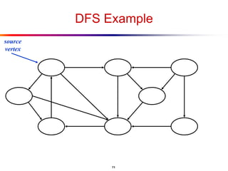
  • 72. 72 DFS Example 1 | | | | | | | | source vertex d f
  • 73. 73 DFS Example 1 | | | | | | 2 | | source vertex d f
  • 74. 74 DFS Example 1 | | | | | 3 | 2 | | source vertex d f
  • 75. 75 DFS Example 1 | | | | | 3 | 4 2 | | source vertex d f
  • 76. 76 DFS Example 1 | | | | 5 | 3 | 4 2 | | source vertex d f
  • 77. 77 DFS Example 1 | | | | 5 | 6 3 | 4 2 | | source vertex d f
  • 78. 78 DFS Example 1 | 8 | | | 5 | 6 3 | 4 2 | 7 | source vertex d f
  • 79. 79 DFS Example 1 | 8 | | | 5 | 6 3 | 4 2 | 7 9 | source vertex d f What is the structure of the grey vertices? What do they represent?
  • 80. 80 DFS Example 1 | 8 | | | 5 | 6 3 | 4 2 | 7 9 |10 source vertex d f
  • 81. 81 DFS Example 1 | 8 |11 | | 5 | 6 3 | 4 2 | 7 9 |10 source vertex d f
  • 82. 82 DFS Example 1 |12 8 |11 | | 5 | 6 3 | 4 2 | 7 9 |10 source vertex d f
  • 83. 83 DFS Example 1 |12 8 |11 13| | 5 | 6 3 | 4 2 | 7 9 |10 source vertex d f
  • 84. 84 DFS Example 1 |12 8 |11 13| 14| 5 | 6 3 | 4 2 | 7 9 |10 source vertex d f
  • 85. 85 DFS Example 1 |12 8 |11 13| 14|15 5 | 6 3 | 4 2 | 7 9 |10 source vertex d f
  • 86. 86 DFS Example 1 |12 8 |11 13|16 14|15 5 | 6 3 | 4 2 | 7 9 |10 source vertex d f
  • 87. 87 DFS: Kinds of edges  DFS introduces an important distinction among edges in the original graph:  Tree edge: encounter new (white) vertex  The tree edges form a spanning forest
  • 88. 88 DFS Example 1 |12 8 |11 13|16 14|15 5 | 6 3 | 4 2 | 7 9 |10 source vertex d f Tree edges
  • 89. 89 DFS: Kinds of edges  DFS introduces an important distinction among edges in the original graph:  Tree edge: encounter new (white) vertex  Back edge: from descendent to ancestor  Encounter a grey vertex (grey to grey)
  • 90. 90 DFS Example 1 |12 8 |11 13|16 14|15 5 | 6 3 | 4 2 | 7 9 |10 source vertex d f Tree edges Back edges
  • 91. 91 DFS: Kinds of edges  DFS introduces an important distinction among edges in the original graph:  Tree edge: encounter new (white) vertex  Back edge: from descendent to ancestor  Forward edge: from ancestor to descendent  Not a tree edge, though  From grey node to black node
  • 92. 92 DFS Example 1 |12 8 |11 13|16 14|15 5 | 6 3 | 4 2 | 7 9 |10 source vertex d f Tree edges Back edges Forward edges
  • 93. 93 DFS: Kinds of edges  DFS introduces an important distinction among edges in the original graph:  Tree edge: encounter new (white) vertex  Back edge: from descendent to ancestor  Forward edge: from ancestor to descendent  Cross edge: between a tree or subtrees  From a grey node to a black node
  • 94. 94 DFS Example 1 |12 8 |11 13|16 14|15 5 | 6 3 | 4 2 | 7 9 |10 source vertex d f Tree edges Back edges Forward edges Cross edges
  • 95. 95 DFS: Kinds of edges  DFS introduces an important distinction among edges in the original graph:  Tree edge: encounter new (white) vertex  Back edge: from descendent to ancestor  Forward edge: from ancestor to descendent  Cross edge: between a tree or subtrees  Note: tree & back edges are important; most algorithms don’t distinguish forward & cross
  • 96. 96 DFS And Graph Cycles  Thm: An undirected graph is acyclic iff a DFS yields no back edges  Thus, can run DFS to find whether a graph has a cycle  What will be the running time?  A: O(V+E)
  • 97. 97 Directed Acyclic Graphs  A directed acyclic graph or DAG is a directed graph with no directed cycles: directed graph G is acyclic iff a DFS of G yields no back edges:
  • 98. 98 Topological Sort  Topological sort of a DAG:  Linear ordering of all vertices in graph G such that vertex u comes before vertex v if edge (u, v)  G  Real-world example: getting dressed
  • 101. 101 Topological Sort Algorithm Topological-Sort() { Run DFS When a vertex is finished, output it Vertices are output in reverse topological order }  Time: O(V+E)
  • 102. 102  G  GT Strongly Connected Components
  • 104. 104 Assignment: Strongly Connected Components 1. Call DFS(G) to compute finishing times f[u] for each vertex u; 2. Compute GT 3. Call DFS(GT), but in the main loop of DFS, consider the vertices in order of decreasing f[u]. 4. Output the vertices for each tree in the depth-first forest of step 3 as a separate strongly connected component.
  • 105. 105 Graphs: Adjacency Matrix  Example: 1 2 4 3 a d b c A 1 2 3 4 1 2 3 ?? 4
  • 106. 106 Graphs: Adjacency Matrix  Example: 1 2 4 3 a d b c A 1 2 3 4 1 0 1 1 0 2 0 0 1 0 3 0 0 0 0 4 0 0 1 0