Machine Learning Algorithms
1 like598 views

This document provides an overview of machine learning algorithms and scikit-learn. It begins with an introduction and table of contents. Then it covers topics like dataset loading from files, pandas, scikit-learn datasets, preprocessing data like handling missing values, feature selection, dimensionality reduction, training and test sets, supervised and unsupervised learning models, and saving/loading machine learning models. For each topic, it provides code examples and explanations.


![1. Dataset Loading: Pandas
Hichem Felouat - hichemfel@gmail.com 3
import pandas as pd
df = pd.DataFrame(
{“a” : [4, 5, 6],
“b” : [7, 8, 9],
“c” : [10, 11, 12]},
index = [1, 2, 3])
a b c
1 4 7 10
2 5 8 11
3 6 9 12](https://image.slidesharecdn.com/machinelearningalgorithms-200927153935/85/Machine-Learning-Algorithms-3-320.jpg)
![1. Dataset Loading: Pandas
Read data from file 'filename.csv'
import pandas as pd
data = pd.read_csv("filename.csv")
print (data)
Select only the feature_1 and feature_2 columns
df = pd.DataFrame(data, columns= ['feature_1',' feature_2 '])
print (df)
Hichem Felouat - hichemfel@gmail.com 4
Data Exploration
# Using head() method with an argument which helps us to restrict the number of initial records
that should be displayed
data.head(n=2)
# Using .tail() method with an argument which helps us to restrict the number of initial records
that should be displayed
data.tail(n=2)](https://image.slidesharecdn.com/machinelearningalgorithms-200927153935/85/Machine-Learning-Algorithms-4-320.jpg)
![Hichem Felouat - hichemfel@gmail.com 5
1. Dataset Loading: Pandas
Training Set & Test Set
columns = [' ', ... , ' '] # n -1
my_data = data[columns ]
# assigning the 'col_i ' column as target
target = data['col_i ' ]
data.head(n=2)
Read and Write to CSV & Excel
df = pd.read_csv('file.csv')
df.to_csv('myDataFrame.csv')
df = pd.read_excel('file.xlsx')
df.to_excel('myDataFrame.xlsx')](https://image.slidesharecdn.com/machinelearningalgorithms-200927153935/85/Machine-Learning-Algorithms-5-320.jpg)


![Hichem Felouat - hichemfel@gmail.com 11
1. Dataset Loading: Scikit Learn
Downloading datasets from the openml.org repository
>>> from sklearn.datasets import fetch_openml
>>> mice = fetch_openml(name='miceprotein', version=4)
>>> mice.data.shape
(1080, 77)
>>> mice.target.shape
(1080,)
>>> np.unique(mice.target)
array(['c-CS-m', 'c-CS-s', 'c-SC-m', 'c-SC-s', 't-CS-m', 't-CS-s', 't-SC-m', 't-SC-s'],
dtype=object)
>>> mice.url
'https://www.openml.org/d/40966'
>>> mice.details['version']
'1'](https://image.slidesharecdn.com/machinelearningalgorithms-200927153935/85/Machine-Learning-Algorithms-11-320.jpg)
![Hichem Felouat - hichemfel@gmail.com 12
1. Dataset Loading: Numpy
Saving & Loading Text Files
import numpy as np
In [1]: a = np.array([1, 2, 3, 4])
In [2]: np.savetxt('test1.txt', a, fmt='%d')
In [3]: b = np.loadtxt('test1.txt', dtype=int)
In [4]: a == b
Out[4]: array([ True, True, True, True], dtype=bool)
# write and read binary files
In [5]: a.tofile('test2.dat')
In [6]: c = np.fromfile('test2.dat', dtype=int)
In [7]: c == a
Out[7]: array([ True, True, True, True], dtype=bool)](https://image.slidesharecdn.com/machinelearningalgorithms-200927153935/85/Machine-Learning-Algorithms-12-320.jpg)
![Hichem Felouat - hichemfel@gmail.com 13
1. Dataset Loading: Numpy
Saving & Loading On Disk
import numpy as np
# .npy extension is added if not given
In [8]: np.save('test3.npy', a)
In [9]: d = np.load('test3.npy')
In [10]: a == d
Out[10]: array([ True, True, True, True], dtype=bool)](https://image.slidesharecdn.com/machinelearningalgorithms-200927153935/85/Machine-Learning-Algorithms-13-320.jpg)
![Hichem Felouat - hichemfel@gmail.com 16
1. Dataset Loading: Generated Datasets -
Clustering
from sklearn.datasets.samples_generator import
make_blobs
from matplotlib import pyplot as plt
import pandas as pd
X, y = make_blobs(n_samples=200, centers=4,
n_features=2)
Xy = pd.DataFrame(dict(x1=X[:,0], x2=X[:,1], label=y))
groups = Xy.groupby('label')
fig, ax = plt.subplots()
colors = ["blue", "red", "green", "purple"]
for idx, classification in groups:
classification.plot(ax=ax, kind='scatter', x='x1', y='x2',
label=idx, color=colors[idx])
plt.show()](https://image.slidesharecdn.com/machinelearningalgorithms-200927153935/85/Machine-Learning-Algorithms-16-320.jpg)
![Hichem Felouat - hichemfel@gmail.com 17
2. Preprocessing Data: missing values
Dealing with missing values :
df = df.fillna('*')
df[‘Test Score’] = df[‘Test Score’].fillna('*')
df[‘Test Score’] = df[‘Test Score'].fillna(df['Test Score'].mean())
df['Test Score'] = df['Test Score'].fillna(df['Test Score'].interpolate())
df= df.dropna() #delete the missing rows of data
df[‘Height(m)']= df[‘Height(m)’].dropna()](https://image.slidesharecdn.com/machinelearningalgorithms-200927153935/85/Machine-Learning-Algorithms-17-320.jpg)
![Hichem Felouat - hichemfel@gmail.com 18
2. Preprocessing Data: missing values
# Dealing with Non-standard missing values:
# dictionary of lists
dictionary = {'Name’:[‘Alex’, ‘Mike’, ‘John’,
‘Dave’, ’Joey’],
‘Height(m)’: [1.75, 1.65, ‘-‘, ‘na’, 1.82],
'Test Score':[70, np.nan, 8, 62, 73]}
# creating a dataframe from list
df = pd.DataFrame(dictionary)
df.isnull()
df = df.replace(['-','na'], np.nan)](https://image.slidesharecdn.com/machinelearningalgorithms-200927153935/85/Machine-Learning-Algorithms-18-320.jpg)
![Hichem Felouat - hichemfel@gmail.com 19
2. Preprocessing Data: missing values
import numpy as np
from sklearn.impute import SimpleImputer
X = [[np.nan, 2], [6, np.nan], [7, 6]]
# mean, median, most_frequent, constant(fill_value = )
imp = SimpleImputer(missing_values = np.nan, strategy='mean')
data = imp.fit_transform(X)
print(data)
Multivariate feature imputation :
IterativeImputer
Nearest neighbors imputation :
KNNImputer
Marking imputed values :
MissingIndicator](https://image.slidesharecdn.com/machinelearningalgorithms-200927153935/85/Machine-Learning-Algorithms-19-320.jpg)

![Hichem Felouat - hichemfel@gmail.com 23
3. Feature Selection: 1. Standardization -
StandardScaler
from sklearn.preprocessing import StandardScaler
import numpy as np
X_train = np.array([[ 1., -1., 2.],
[ 2., 0., 0.],
[ 0., 1., -1.]])
scaler = StandardScaler().fit_transform(X_train)
print(scaler)
Out:
[[ 0. -1.22474487 1.33630621]
[ 1.22474487 0. -0.26726124]
[-1.22474487 1.22474487 -1.06904497]]](https://image.slidesharecdn.com/machinelearningalgorithms-200927153935/85/Machine-Learning-Algorithms-23-320.jpg)
![Hichem Felouat - hichemfel@gmail.com 24
3. Feature Selection: 1. Standardization -
Scaling Features to a Range
import numpy as np
from sklearn import preprocessing
X_train = np.array([[ 1., -1., 2.], [ 2., 0., 0.], [ 0., 1., -1.]])
# Here is an example to scale a data matrix to the [0, 1] range:
min_max_scaler = preprocessing.MinMaxScaler()
X_train_minmax = min_max_scaler.fit_transform(X_train)
print(X_train_minmax)
# between a given minimum and maximum value
min_max_scaler = preprocessing.MinMaxScaler(feature_range=(0, 10))
# scaling in a way that the training data lies within the range [-1, 1]
max_abs_scaler = preprocessing.MaxAbsScaler()](https://image.slidesharecdn.com/machinelearningalgorithms-200927153935/85/Machine-Learning-Algorithms-24-320.jpg)
![Hichem Felouat - hichemfel@gmail.com 25
3. Feature Selection: 1. Standardization - Scaling Data
with Outliers
If your data contains many outliers, scaling using the mean and variance of the
data is likely to not work very well. In these cases, you can use robust_scale
and RobustScaler as drop-in replacements instead. They use more robust
estimates for the center and range of your data.
import numpy as np
from sklearn import preprocessing
X_train = np.array([[ 1., -1., 2.], [ 2., 0., 0.], [ 0., 1., -1.]])
scaler = preprocessing.RobustScaler()
X_train_rob_scal = scaler.fit_transform(X_train)
print(X_train_rob_scal)](https://image.slidesharecdn.com/machinelearningalgorithms-200927153935/85/Machine-Learning-Algorithms-25-320.jpg)
![Hichem Felouat - hichemfel@gmail.com 26
3. Feature Selection: 2. Non-linear Transformation -
Mapping to a Uniform Distribution
QuantileTransformer and quantile_transform provide a non-parametric
transformation to map the data to a uniform distribution with values between 0
and 1:
from sklearn.datasets import load_iris
from sklearn.model_selection import train_test_split
from sklearn import preprocessing
import numpy as np
X, y = load_iris(return_X_y=True)
X_train, X_test, y_train, y_test = train_test_split(X, y, random_state=0)
print(X_train)
quantile_transformer = preprocessing.QuantileTransformer(random_state=0)
X_train_trans = quantile_transformer.fit_transform(X_train)
print(X_train_trans)
X_test_trans = quantile_transformer.transform(X_test)
# Compute the q-th percentile of the data along the specified axis.
np.percentile(X_train[:, 0], [0, 25, 50, 75, 100])](https://image.slidesharecdn.com/machinelearningalgorithms-200927153935/85/Machine-Learning-Algorithms-26-320.jpg)
![Hichem Felouat - hichemfel@gmail.com 28
3. Feature Selection: 3. Normalization
Normalization is the process of scaling individual samples to have
unit norm. This process can be useful if you plan to use a quadratic
form such as the dot-product or any other kernel to quantify the
similarity of any pair of samples.
from sklearn import preprocessing
import numpy as np
X = [[ 1., -1., 2.], [ 2., 0., 0.], [ 0., 1., -1.]]
X_normalized = preprocessing.normalize(X, norm='l2')
print(X_normalized)](https://image.slidesharecdn.com/machinelearningalgorithms-200927153935/85/Machine-Learning-Algorithms-28-320.jpg)
![Hichem Felouat - hichemfel@gmail.com 29
3. Feature Selection: 4. Encoding
Categorical Features
To convert categorical features to such integer codes, we can use the
OrdinalEncoder. This estimator transforms each categorical feature to one
new feature of integers (0 to n_categories - 1).
from sklearn import preprocessing
#genders = ['female', 'male']
#locations = ['from Africa', 'from Asia', 'from Europe', 'from US']
#browsers = ['uses Chrome', 'uses Firefox', 'uses IE', 'uses Safari']
X = [['male', 'from US', 'uses Safari'], ['female', 'from Europe', 'uses Safari'],
['female', 'from Asia', 'uses Firefox'], ['male', 'from Africa', 'uses
Chrome']]
enc = preprocessing.OrdinalEncoder()
X_enc = enc.fit_transform(X)
print(X_enc)](https://image.slidesharecdn.com/machinelearningalgorithms-200927153935/85/Machine-Learning-Algorithms-29-320.jpg)

![Hichem Felouat - hichemfel@gmail.com 31
3. Feature Selection: 5. Discretization
from sklearn import preprocessing
import numpy as np
X = np.array([[ -3., 5., 15 ],
[ 0., 6., 14 ],
[ 6., 3., 11 ]])
# 'onehot’, ‘onehot-dense’, ‘ordinal’
kbd = preprocessing.KBinsDiscretizer(n_bins=[3, 2, 2],
encode='ordinal')
X_kbd = kbd.fit_transform(X)
print(X_kbd)](https://image.slidesharecdn.com/machinelearningalgorithms-200927153935/85/Machine-Learning-Algorithms-31-320.jpg)
![Hichem Felouat - hichemfel@gmail.com 32
3. Feature Selection: 5.1 Feature
Binarization
from sklearn import preprocessing
import numpy as np
X = [[ 1., -1., 2.],[ 2., 0., 0.],[ 0., 1., -1.]]
binarizer = preprocessing.Binarizer()
X_bin = binarizer.fit_transform(X)
print(X_bin)
# It is possible to adjust the threshold of the binarizer:
binarizer_1 = preprocessing.Binarizer(threshold=1.1)
X_bin_1 = binarizer_1.fit_transform(X)
print(X_bin_1)](https://image.slidesharecdn.com/machinelearningalgorithms-200927153935/85/Machine-Learning-Algorithms-32-320.jpg)


![Hichem Felouat - hichemfel@gmail.com 35
3. Feature Selection: 7. Custom
Transformers
Often, you will want to convert an existing Python function into a transformer to
assist in data cleaning or processing. You can implement a transformer from an
arbitrary function with FunctionTransformer. For example, to build a transformer
that applies a log transformation in a pipeline, do:
from sklearn import preprocessing
import numpy as np
transformer = preprocessing.FunctionTransformer(np.log1p,
validate=True)
X = np.array([[0, 1], [2, 3]])
X_tr = transformer.fit_transform(X)
print(X_tr)](https://image.slidesharecdn.com/machinelearningalgorithms-200927153935/85/Machine-Learning-Algorithms-35-320.jpg)


![Hichem Felouat - hichemfel@gmail.com 38
from sklearn.feature_extraction.text import CountVectorizer
texts = [
"blue car and blue window",
"black crow in the window",
"i see my reflection in the window"
]
vec = CountVectorizer(binary=True)
vec.fit(texts)
print([w for w in sorted(vec.vocabulary_.keys())])
X = vec.transform(texts).toarray()
print(X)
import pandas as pd
pd.DataFrame(vec.transform(texts).toarray(), columns=sorted(vec.vocabulary_.keys()))
3. Feature Selection: Text Feature](https://image.slidesharecdn.com/machinelearningalgorithms-200927153935/85/Machine-Learning-Algorithms-38-320.jpg)
![Hichem Felouat - hichemfel@gmail.com 39
bigram_vectorizer = CountVectorizer(ngram_range=(1, 2),
token_pattern=r'bw+b', min_df=1)
analyze = bigram_vectorizer.build_analyzer()
analyze('Bi-grams are cool!') == (
['bi', 'grams', 'are', 'cool', 'bi grams', 'grams are', 'are cool'])
3. Feature Selection: Text Feature
To preserve some of the local ordering information we can extract 2-grams of
words in addition to the 1-grams (individual words):](https://image.slidesharecdn.com/machinelearningalgorithms-200927153935/85/Machine-Learning-Algorithms-39-320.jpg)


![Hichem Felouat - hichemfel@gmail.com 42
3. Feature Selection: Text Feature
from sklearn.feature_extraction.text import TfidfVectorizer
texts = [
"blue car and blue window",
"black crow in the window",
"i see my reflection in the window"
]
vec = TfidfVectorizer()
vec.fit(texts)
print([w for w in sorted(vec.vocabulary_.keys())])
X = vec.transform(texts).toarray()
import pandas as pd
pd.DataFrame(vec.transform(texts).toarray(),
columns=sorted(vec.vocabulary_.keys()))](https://image.slidesharecdn.com/machinelearningalgorithms-200927153935/85/Machine-Learning-Algorithms-42-320.jpg)
![Hichem Felouat - hichemfel@gmail.com 43
3. Feature Selection: Image Feature
#image.extract_patches_2d
from sklearn.feature_extraction import image
from sklearn.datasets import fetch_olivetti_faces
import matplotlib.pyplot as plt
import matplotlib.image as img
data = fetch_olivetti_faces()
plt.imshow(data.images[0])
patches = image.extract_patches_2d(data.images[0], (2, 2),
max_patches=2,random_state=0)
print('Image shape: {}'.format(data.images[0].shape),' Patches shape:
{}'.format(patches.shape))
print('Patches = ',patches)](https://image.slidesharecdn.com/machinelearningalgorithms-200927153935/85/Machine-Learning-Algorithms-43-320.jpg)
![Hichem Felouat - hichemfel@gmail.com 44
3. Feature Selection: Image Feature
import cv2
def hu_moments(image):
image = cv2.cvtColor(image, cv2.COLOR_BGR2GRAY)
feature = cv2.HuMoments(cv2.moments(image)).flatten()
return feature
def histogram(image,mask=None):
image = cv2.cvtColor(image, cv2.COLOR_BGR2HSV)
hist = cv2.calcHist([image],[0],None,[256],[0,256])
cv2.normalize(hist, hist)
return hist.flatten()](https://image.slidesharecdn.com/machinelearningalgorithms-200927153935/85/Machine-Learning-Algorithms-44-320.jpg)


![Hichem Felouat - hichemfel@gmail.com 55
from sklearn.model_selection import train_test_split
import matplotlib.pyplot as plt
from mpl_toolkits.mplot3d import Axes3D
from sklearn import datasets, linear_model
from sklearn import metrics
import numpy as np
dat = datasets.load_boston()
X = dat.data
Y = dat.target
print("Examples = ",X.shape ," Labels = ", Y.shape)
fig, ax = plt.subplots(figsize=(12,8))
ax.scatter(X[:,0], Y, edgecolors=(0, 0, 0))
ax.plot([Y.min(), Y.max()], [Y.min(), Y.max()], 'k--', lw=4)
ax.set_xlabel('F')
ax.set_ylabel('Y')
plt.show()
fig = plt.figure(figsize=(12, 8))
ax = fig.add_subplot(111, projection='3d')
ax.scatter(X[:, 0], X[:, 1], Y, c='b', marker='o',cmap=plt.cm.Set1, edgecolor='k', s=40)
ax.set_title("My Data")
ax.set_xlabel("F1")
ax.w_xaxis.set_ticklabels([])
ax.set_ylabel("F2")
ax.w_yaxis.set_ticklabels([])
ax.set_zlabel("Y")
ax.w_zaxis.set_ticklabels([])
plt.show()
X_train, X_test, Y_train, Y_test = train_test_split(X,
Y, test_size= 0.20, random_state=100)
print("X_train = ",X_train.shape ," Y_test = ", Y_test.shape)
regressor = linear_model.LinearRegression()
regressor.fit(X_train, Y_train)
predicted = regressor.predict(X_test)
import pandas as pd
df = pd.DataFrame({'Actual': Y_test.flatten(), 'Predicted': predicted.flatten()})
print(df)
df1 = df.head(25)
df1.plot(kind='bar',figsize=(12,8))
plt.grid(which='major', linestyle='-', linewidth='0.5', color='green')
plt.grid(which='minor', linestyle=':', linewidth='0.5', color='black')
plt.show()
predicted_all = regressor.predict(X)
fig, ax = plt.subplots(figsize=(12,8))
ax.scatter(X[:,0], Y, edgecolors=(0, 0, 1))
ax.scatter(X[:,0], predicted_all, edgecolors=(1, 0, 0))
ax.set_xlabel('Measured')
ax.set_ylabel('Predicted')
plt.show()
fig = plt.figure(figsize=(12, 8))
ax = fig.add_subplot(111, projection='3d')
ax.scatter(X[:, 0], X[:, 1], Y, c='b', marker='o',cmap=plt.cm.Set1, edgecolor='k', s=40)
ax.scatter(X[:, 0], X[:, 1], predicted_all, c='r', marker='o',cmap=plt.cm.Set1, edgecolor='k',
s=40)
ax.set_title("My Data")
ax.set_xlabel("F1")
ax.w_xaxis.set_ticklabels([])
ax.set_ylabel("F2")
ax.w_yaxis.set_ticklabels([])
ax.set_zlabel("Y")
ax.w_zaxis.set_ticklabels([])
plt.show()
print('Mean Absolute Error : ', metrics.mean_absolute_error(Y_test, predicted))
print('Mean Squared Error : ', metrics.mean_squared_error(Y_test, predicted))
print('Root Mean Squared Error: ', np.sqrt(metrics.mean_squared_error(Y_test, predicted)))](https://image.slidesharecdn.com/machinelearningalgorithms-200927153935/85/Machine-Learning-Algorithms-55-320.jpg)
![Hichem Felouat - hichemfel@gmail.com 56
1. Regression: Learning Curves
def plot_learning_curves(model, X, y):
from sklearn.metrics import mean_squared_error
X_train, X_val, y_train, y_val = train_test_split(X, y, test_size=0.2)
train_errors, val_errors = [], []
for m in range(1, len(X_train)):
model.fit(X_train[:m], y_train[:m])
y_train_predict = model.predict(X_train[:m])
y_val_predict = model.predict(X_val)
train_errors.append(mean_squared_error(y_train_predict, y_train[:m]))
val_errors.append(mean_squared_error(y_val_predict, y_val))
fig, ax = plt.subplots(figsize=(12,8))
ax.plot(np.sqrt(train_errors), "r-+", linewidth=2, label="train")
ax.plot(np.sqrt(val_errors), "b-", linewidth=3, label="val")
ax.legend(loc='upper right', bbox_to_anchor=(0.5, 1.1),ncol=1, fancybox=True, shadow=True)
ax.set_xlabel('Training set size')
ax.set_ylabel('RMSE')
plt.show()](https://image.slidesharecdn.com/machinelearningalgorithms-200927153935/85/Machine-Learning-Algorithms-56-320.jpg)

![Hichem Felouat - hichemfel@gmail.com 58
1. Regression: Kernel Ridge regression
from sklearn.kernel_ridge import KernelRidge
# kernel = [linear,polynomial,rbf]
regressor = KernelRidge(kernel ='rbf', alpha=1.0)
regressor.fit(X_train, Y_train)
predicted = regressor.predict(X_test)
In order to explore nonlinear relations of the regression problem](https://image.slidesharecdn.com/machinelearningalgorithms-200927153935/85/Machine-Learning-Algorithms-58-320.jpg)

![Hichem Felouat - hichemfel@gmail.com 60
1. Regression: Polynomial Regression
# generate some nonlinear data
import numpy as np
m = 1000
X = 6 * np.random.rand(m, 1) - 3
Y = 0.5 * X**2 + X + 2 + np.random.randn(m, 1)
print("Examples = ",X.shape ," Labels = ", Y.shape)
import matplotlib.pyplot as plt
from mpl_toolkits.mplot3d import Axes3D
fig, ax = plt.subplots(figsize=(12,8))
ax.scatter(X[:,0], Y, edgecolors=(0, 0, 1))
ax.set_xlabel('F')
ax.set_ylabel('Y')
plt.show()
from sklearn.preprocessing import PolynomialFeatures
poly_features = PolynomialFeatures(degree=2,
include_bias=False)
X_poly = poly_features.fit_transform(X)
print("Examples = ",X_poly.shape ," Labels = ", Y.shape)
from sklearn.model_selection import train_test_split
X_train, X_test, Y_train, Y_test = train_test_split(X_poly,
Y, test_size= 0.20, random_state=100)
from sklearn import linear_model
regressor = linear_model.LinearRegression()
regressor.fit(X_train, Y_train)
predicted = regressor.predict(X_poly)
fig, ax = plt.subplots(figsize=(12,8))
ax.scatter(X, Y, edgecolors=(0, 0, 1))
ax.scatter(X,predicted,edgecolors=(1, 0, 0))
ax.set_xlabel('F')
ax.set_ylabel('Y')
plt.show()
B = regressor.intercept_
A = regressor.coef_
print(A)
print(B)
print("The model estimates : Y = ",B[0]," + ",A[0,0]," X + ",A[0,1]," X^2")
from sklearn import metrics
predicted = regressor.predict(X_test)
print('Mean Absolute Error : ', metrics.mean_absolute_error(Y_test, predicted))
print('Mean Squared Error : ', metrics.mean_squared_error(Y_test, predicted))
print('Root Mean Squared Error: ', np.sqrt(metrics.mean_squared_error(Y_test,
predicted)))](https://image.slidesharecdn.com/machinelearningalgorithms-200927153935/85/Machine-Learning-Algorithms-60-320.jpg)

![Hichem Felouat - hichemfel@gmail.com 62
1. Regression: Support Vector Regression
SVR
import numpy as np
from sklearn.svm import SVR
import matplotlib.pyplot as plt
# Generate sample data
X = np.sort(5 * np.random.rand(40, 1), axis=0)
Y = np.sin(X).ravel()
# Add noise to targets
Y[::5] += 3 * (0.5 - np.random.rand(8))
print("Examples = ",X.shape ," Y = ", Y.shape)
# Fit regression model
svr_rbf = SVR(kernel='rbf', C=100, gamma=0.1, epsilon=.1)
svr_lin = SVR(kernel='linear', C=100, gamma='auto')
svr_poly = SVR(kernel='poly', C=100, gamma='auto', degree=3,
epsilon=.1, coef0=1)
# Look at the results
lw = 2
svrs = [svr_rbf, svr_lin, svr_poly]
kernel_label = ['RBF', 'Linear', 'Polynomial']
model_color = ['m', 'c', 'g']
fig, axes = plt.subplots(nrows=1, ncols=3, figsize=(15, 10), sharey=True)
for ix, svr in enumerate(svrs):
axes[ix].plot(X, svr.fit(X, Y).predict(X), color=model_color[ix], lw=lw,
label='{} model'.format(kernel_label[ix]))
axes[ix].scatter(X[svr.support_], Y[svr.support_], facecolor="none",
edgecolor=model_color[ix], s=50,
label='{} support vectors'.format(kernel_label[ix]))
axes[ix].scatter(X[np.setdiff1d(np.arange(len(X)), svr.support_)],
Y[np.setdiff1d(np.arange(len(X)), svr.support_)],
facecolor="none", edgecolor="k", s=50,
label='other training data')
axes[ix].legend(loc='upper center', bbox_to_anchor=(0.5, 1.1),
ncol=1, fancybox=True, shadow=True)
fig.text(0.5, 0.04, 'data', ha='center', va='center')
fig.text(0.06, 0.5, 'target', ha='center', va='center', rotation='vertical')
fig.suptitle("Support Vector Regression", fontsize=14)
plt.show()](https://image.slidesharecdn.com/machinelearningalgorithms-200927153935/85/Machine-Learning-Algorithms-62-320.jpg)

![Hichem Felouat - hichemfel@gmail.com 64
1. Regression: Decision Trees Regression
import matplotlib.pyplot as plt
import numpy as np
from sklearn.tree import DecisionTreeRegressor
rng = np.random.RandomState(1)
X = np.sort(5 * rng.rand(80, 1), axis=0)
Y = np.sin(X).ravel()
Y[::5] += 3 * (0.5 - rng.rand(16))
print("Examples = ",X.shape ," Labels = ", Y.shape)
X_test = np.arange(0.0, 5.0, 0.01)[:, np.newaxis]
regressor1 = DecisionTreeRegressor(max_depth=2)
regressor2 = DecisionTreeRegressor(max_depth=5)
regressor1.fit(X, Y)
regressor2.fit(X, Y)
predicted1 = regressor1.predict(X_test)
predicted2 = regressor2.predict(X_test)
plt.figure(figsize=(12,8))
plt.scatter(X, Y, s=20, edgecolor="black",c="darkorange",
label="data")
plt.plot(X_test, predicted1,
color="cornflowerblue",label="max_depth=2", linewidth=2)
plt.plot(X_test, predicted2, color="yellowgreen",
label="max_depth=5", linewidth=2)
plt.xlabel("data")
plt.ylabel("target")
plt.title("Decision Tree Regression")
plt.legend()
plt.show()](https://image.slidesharecdn.com/machinelearningalgorithms-200927153935/85/Machine-Learning-Algorithms-64-320.jpg)


![Hichem Felouat - hichemfel@gmail.com 70
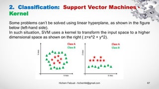
2. Classification: Support Vector Machines -Kernel +
Tuning Hyperparameters
import matplotlib.pyplot as plt
from sklearn import datasets, svm, metrics
from sklearn.model_selection import train_test_split
digits = datasets.load_digits()
_, axes = plt.subplots(2, 4)
images_and_labels = list(zip(digits.images, digits.target))
for ax, (image, label) in zip(axes[0, :], images_and_labels[:4]):
ax.set_axis_off()
ax.imshow(image, cmap=plt.cm.gray_r,
interpolation='nearest')
ax.set_title('Training: %i' % label)
# To apply a classifier on this data, we need to flatten the image,
to
# turn the data in a (samples, feature) matrix:
n_samples = len(digits.images)
data = digits.images.reshape((n_samples, -1))
# Create a classifier: a support vector classifier
classifier = svm.SVC(gamma=0.001)
# Split data into train and test subsets
X_train, X_test, y_train, y_test = train_test_split(
data, digits.target, test_size=0.5, shuffle=False)
# We learn the digits on the first half of the digits
classifier.fit(X_train, y_train)
# Now predict the value of the digit on the second half:
predicted = classifier.predict(X_test)
images_and_predictions = list(zip(digits.images[n_samples // 2:], predicted))
for ax, (image, prediction) in zip(axes[1, :], images_and_predictions[:4]):
ax.set_axis_off()
ax.imshow(image, cmap=plt.cm.gray_r, interpolation='nearest')
ax.set_title('Prediction: %i' % prediction)
print("Classification report : n", classifier,"n",
metrics.classification_report(y_test, predicted))
disp = metrics.plot_confusion_matrix(classifier, X_test, y_test)
disp.figure_.suptitle("Confusion Matrix")
print("Confusion matrix: n", disp.confusion_matrix)
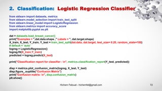
plt.show()](https://image.slidesharecdn.com/machinelearningalgorithms-200927153935/85/Machine-Learning-Algorithms-70-320.jpg)


![Hichem Felouat - hichemfel@gmail.com 76
2. Classification: Stochastic Gradient Descent
from sklearn.linear_model import SGDClassifier
X = [[0., 0.], [1., 1.]]
y = [0, 1]
# loss : hinge, log, modified_huber, squared_hinge, perceptron
clf = SGDClassifier(loss="hinge", penalty="l2", max_iter=5)
clf.fit(X, y)
predicted = clf.predict(X_test)](https://image.slidesharecdn.com/machinelearningalgorithms-200927153935/85/Machine-Learning-Algorithms-76-320.jpg)

![Hichem Felouat - hichemfel@gmail.com 78
from sklearn.neighbors import KNeighborsClassifier
from sklearn.model_selection import train_test_split
from sklearn.datasets import load_iris
from sklearn.metrics import classification_report,
confusion_matrix
import numpy as np
import matplotlib.pyplot as plt
# Loading data
irisData = load_iris()
# Create feature and target arrays
X = irisData.data
y = irisData.target
# Split into training and test set
X_train, X_test, y_train, y_test = train_test_split(
X, y, test_size = 0.2, random_state=42)
knn = KNeighborsClassifier(n_neighbors = 7)
knn.fit(X_train, y_train)
predicted = knn.predict(X_test)
print(confusion_matrix(y_test, predicted))
print(classification_report(y_test, predicted))
2. Classification: K-Nearest Neighbors KNN
neighbors = np.arange(1, 25)
train_accuracy = np.empty(len(neighbors))
test_accuracy = np.empty(len(neighbors))
# Loop over K values
for i, k in enumerate(neighbors):
knn = KNeighborsClassifier(n_neighbors=k)
knn.fit(X_train, y_train)
# Compute traning and test data accuracy
train_accuracy[i] = knn.score(X_train, y_train)
test_accuracy[i] = knn.score(X_test, y_test)
# Generate plot
plt.plot(neighbors, test_accuracy, label = 'Testing dataset
Accuracy')
plt.plot(neighbors, train_accuracy, label = 'Training
dataset Accuracy')
plt.legend()
plt.xlabel('n_neighbors')
plt.ylabel('Accuracy')
plt.show()](https://image.slidesharecdn.com/machinelearningalgorithms-200927153935/85/Machine-Learning-Algorithms-78-320.jpg)


![Hichem Felouat - hichemfel@gmail.com 84
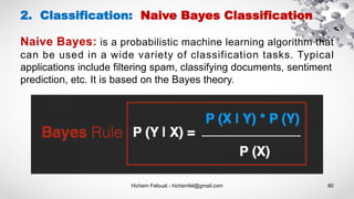
2. Classification: Naive Bayes Classification
# Assigning features and label variables
weather=['Sunny','Sunny','Overcast','Rainy','Rainy','R
ainy','Overcast','Sunny','Sunny',
'Rainy','Sunny','Overcast','Overcast','Rainy']
temp=['Hot','Hot','Hot','Mild','Cool','Cool','Cool','Mild','
Cool','Mild','Mild','Mild','Hot','Mild']
play=['No','No','Yes','Yes','Yes','No','Yes','No','Yes','Ye
s','Yes','Yes','No','No']
# Import LabelEncoder
from sklearn import preprocessing
# creating labelEncoder
le = preprocessing.LabelEncoder()
# Converting string labels into numbers.
weather_encoded=le.fit_transform(weather)
print("weather:",wheather_encoded)
# Converting string labels into numbers
temp_encoded=le.fit_transform(temp)
label=le.fit_transform(play)
print("Temp: ",temp_encoded)
print("Play: ",label)
# Combinig weather and temp into single listof tuples
features = zip(weather_encoded,temp_encoded)
import numpy as np
features = np.asarray(list(features))
print("features : ",features)
#Import Gaussian Naive Bayes model
from sklearn.naive_bayes import GaussianNB
#Create a Gaussian Classifier
model = GaussianNB()
# Train the model using the training sets
model.fit(features,label)
# Predict Output
predicted= model.predict([[0,2]]) # 0:Overcast, 2:Mild
print ("Predicted Value (No = 0, Yes = 1):", predicted)](https://image.slidesharecdn.com/machinelearningalgorithms-200927153935/85/Machine-Learning-Algorithms-84-320.jpg)

![Hichem Felouat - hichemfel@gmail.com 86
2. Classification: Gaussian Naive Bayes Classification
# load the iris dataset
from sklearn.datasets import load_iris
iris = load_iris()
# store the feature matrix (X) and response vector (y)
X = iris.data
y = iris.target
# splitting X and y into training and testing sets
from sklearn.model_selection import train_test_split
X_train, X_test, y_train, y_test = train_test_split(X, y, test_size=0.4, random_state=100)
# training the model on training set
from sklearn.naive_bayes import GaussianNB
gnb = GaussianNB()
gnb.fit(X_train, y_train)
# making predictions on the testing set
y_pred = gnb.predict(X_test)
# comparing actual response values (y_test) with predicted response values (y_pred)
from sklearn import metrics
print("Gaussian Naive Bayes model accuracy(in %):", metrics.accuracy_score(y_test, y_pred)*100)
print("Number of mislabeled points out of a total %d points : %d" % (X_test.shape[0], (y_test !=
y_pred).sum()))](https://image.slidesharecdn.com/machinelearningalgorithms-200927153935/85/Machine-Learning-Algorithms-86-320.jpg)

![Hichem Felouat - hichemfel@gmail.com 88
2. Classification: Multinomial Naive Bayes
Classification
from sklearn.datasets import fetch_20newsgroups
data = fetch_20newsgroups()
print(data.target_names)
# For simplicity here, we will select just a few of these categories
categories = ['talk.religion.misc', 'soc.religion.christian',
'sci.space', 'comp.graphics']
sub_data = fetch_20newsgroups(subset='train',
categories=categories)
X, Y = sub_data.data, sub_data.target
print("Examples = ",len(X)," Labels = ", len(Y))
# Here is a representative entry from the data:
print(X[5])
# In order to use this data for machine learning, we need to be
able to convert the content of each string into a vector of numbers.
# For this we will use the TF-IDF vectorizer
from sklearn.feature_extraction.text import TfidfVectorizer
vec = TfidfVectorizer()
vec.fit(X)
texts = vec.transform(X).toarray()
print(" texts shape = ",texts.shape)
# split the dataset into training data and test data
from sklearn.model_selection import train_test_split
X_train, X_test, Y_train, Y_test = train_test_split(texts, Y,
test_size= 0.20, random_state=100, stratify=Y)
# training the model on training set
from sklearn.naive_bayes import MultinomialNB
clf = MultinomialNB()
clf.fit(X_train, Y_train)
# making predictions on the testing set
predicted = clf.predict(X_test)
from sklearn import metrics
print("Classification report : n", clf,"n",
metrics.classification_report(Y_test, predicted))
disp = metrics.plot_confusion_matrix(clf, X_test, Y_test)
disp.figure_.suptitle("Confusion Matrix")
print("Confusion matrix: n", disp.confusion_matrix)](https://image.slidesharecdn.com/machinelearningalgorithms-200927153935/85/Machine-Learning-Algorithms-88-320.jpg)


![Hichem Felouat - hichemfel@gmail.com 94
2. Classification: Decision Trees - Example
# Visualize data
import collections
import pydotplus
dot_data = tree.export_graphviz(tree_clf, feature_names=dat.feature_names, out_file=None, filled=True, rounded=True)
graph = pydotplus.graph_from_dot_data(dot_data)
colors = ('turquoise', 'orange')
edges = collections.defaultdict(list)
for edge in graph.get_edge_list():
edges[edge.get_source()].append(int(edge.get_destination()))
for edge in edges:
edges[edge].sort()
for i in range(2):
dest = graph.get_node(str(edges[edge][i]))[0]
dest.set_fillcolor(colors[i])
graph.write_png('tree1.png')
#pdf
import graphviz
dot_data = tree.export_graphviz(tree_clf, out_file=None)
graph = graphviz.Source(dot_data)
graph.render("iris")
dot_data = tree.export_graphviz(tree_clf, out_file=None, feature_names=dat.feature_names, class_names=dat.target_names,
filled=True, rounded=True, special_characters=True)
graph = graphviz.Source(dot_data)
graph.view('tree2.pdf')](https://image.slidesharecdn.com/machinelearningalgorithms-200927153935/85/Machine-Learning-Algorithms-94-320.jpg)


![Hichem Felouat - hichemfel@gmail.com 97
Estimating Class Probabilities:
A Decision Tree can also estimate the probability that an instance belongs to a
particular class k: first it traverses the tree to find the leaf node for this instance,
and then it returns the ratio of training instances of class k in this node.
2. Classification: Decision Trees
print("predict_proba : ",tree_clf.predict_proba([[1, 1.5, 3.2, 0.5]]))
predict_proba : [[0. 0.91489362 0.08510638]]
Scikit-Learn uses the CART algorithm, which produces only binary trees:
nonleaf nodes always have two children (i.e., questions only have yes/no
answers). However, other algorithms such as ID3 can produce Decision Trees
with nodes that have more than two children.](https://image.slidesharecdn.com/machinelearningalgorithms-200927153935/85/Machine-Learning-Algorithms-97-320.jpg)


![Hichem Felouat - hichemfel@gmail.com 103
from sklearn import datasets
from sklearn.model_selection import train_test_split
from sklearn.ensemble import RandomForestClassifier, VotingClassifier
from sklearn.linear_model import LogisticRegression
from sklearn.svm import SVC
from sklearn.metrics import accuracy_score
dat = datasets.load_breast_cancer()
print("Examples = ",dat.data.shape ," Labels = ", dat.target.shape)
X_train, X_test, Y_train, Y_test = train_test_split(dat.data,
dat.target, test_size= 0.20, random_state=100)
log_clf = LogisticRegression()
rnd_clf = RandomForestClassifier()
svm_clf = SVC()
voting_clf = VotingClassifier(
estimators=[('lr', log_clf), ('rf', rnd_clf), ('svc', svm_clf)],voting='hard')
voting_clf.fit(X_train, Y_train)
for clf in (log_clf, rnd_clf, svm_clf, voting_clf):
clf.fit(X_train, Y_train)
y_pred = clf.predict(X_test)
print(clf.__class__.__name__, accuracy_score(Y_test, y_pred))
3. Ensemble Methods: Voting Classifier](https://image.slidesharecdn.com/machinelearningalgorithms-200927153935/85/Machine-Learning-Algorithms-103-320.jpg)

![Hichem Felouat - hichemfel@gmail.com 105
3. Ensemble Methods: Voting Classifier - (Soft Voting)
from sklearn import datasets
from sklearn.tree import DecisionTreeClassifier
from sklearn.neighbors import KNeighborsClassifier
from sklearn.svm import SVC
from itertools import product
from sklearn.ensemble import VotingClassifier
from sklearn.model_selection import train_test_split
# Loading some example data
dat = datasets.load_iris()
X_train, X_test, Y_train, Y_test = train_test_split(dat.data, dat.target, test_size= 0.20, random_state=100)
# Training classifiers
clf1 = DecisionTreeClassifier(max_depth=4)
clf2 = KNeighborsClassifier(n_neighbors=7)
clf3 = SVC(kernel='rbf', probability=True)
voting_clf_soft = VotingClassifier(estimators=[('dt', clf1), ('knn', clf2), ('svc', clf3)],
voting='soft', weights=[2, 1, 3])
for clf in (clf1, clf2, clf3, voting_clf_soft):
clf.fit(X_train, Y_train)
y_pred = clf.predict(X_test)
print(clf.__class__.__name__, accuracy_score(Y_test, y_pred))](https://image.slidesharecdn.com/machinelearningalgorithms-200927153935/85/Machine-Learning-Algorithms-105-320.jpg)
![Hichem Felouat - hichemfel@gmail.com 106
from sklearn.datasets import load_boston
from sklearn.ensemble import GradientBoostingRegressor, RandomForestRegressor,VotingRegressor
from sklearn.linear_model import LinearRegression
from sklearn.model_selection import train_test_split
from sklearn import metrics
import numpy as np
# Loading some example data
dat = load_boston()
X_train, X_test, Y_train, Y_test = train_test_split(dat.data,
dat.target, test_size= 0.20, random_state=100)
# Training classifiers
reg1 = GradientBoostingRegressor(random_state=1, n_estimators=10)
reg2 = RandomForestRegressor(random_state=1, n_estimators=10)
reg3 = LinearRegression()
voting_reg = VotingRegressor(estimators=[('gb', reg1), ('rf', reg2), ('lr', reg3)], weights=[1, 3, 2])
for clf in (reg1, reg2, reg3, voting_reg):
clf.fit(X_train, Y_train)
y_pred = clf.predict(X_test)
print(clf.__class__.__name__," : **********")
print('Mean Absolute Error : ', metrics.mean_absolute_error(Y_test, y_pred))
print('Mean Squared Error : ', metrics.mean_squared_error(Y_test, y_pred))
print('Root Mean Squared Error: ', np.sqrt(metrics.mean_squared_error(Y_test, y_pred)))
3. Ensemble Methods: Voting Regressor](https://image.slidesharecdn.com/machinelearningalgorithms-200927153935/85/Machine-Learning-Algorithms-106-320.jpg)


![Hichem Felouat - hichemfel@gmail.com 115
3. Ensemble Methods: XGBoost - Classification
from sklearn.datasets import load_iris
from sklearn.model_selection import train_test_split
X, y = load_iris(return_X_y=True)
X_train, X_test, y_train, y_test = train_test_split(X,
y, test_size= 0.20, random_state=100)
# In order for XGBoost to be able to use our data,
# we’ll need to transform it into a specific format that XGBoost can handle.
D_train = xgb.DMatrix(X_train, label=y_train)
D_test = xgb.DMatrix(X_test, label=y_test)
# Training classsifier
import xgboost as xgb
param = {'eta': 0.3, 'max_depth': 3, 'objective':
'multi:softprob',
'num_class': 3}
steps = 20 # The number of training iterations
xg_clf = xgb.train(param, D_train, steps)
# making predictions on the testing set
predicted = xg_reg.predict(X_test)
# comparing actual response values (y_test) with predicted response values (predicted)
from sklearn import metrics
print("Classification report : n", xg_clf,"n", metrics.classification_report(y_test, predicted))
disp.figure_.suptitle("Confusion Matrix")
print("Confusion matrix: n", disp.confusion_matrix)
# Visualize Boosting Trees and
# Feature Importance
import matplotlib.pyplot as plt
xgb.plot_tree(xg_clf,num_trees=0)
plt.rcParams['figure.figsize'] = [10,
10]
plt.show()
xgb.plot_importance(xg_clf)
plt.rcParams['figure.figsize'] = [5, 5]
plt.show()](https://image.slidesharecdn.com/machinelearningalgorithms-200927153935/85/Machine-Learning-Algorithms-115-320.jpg)


![Hichem Felouat - hichemfel@gmail.com 121
4. Cross-Validation
import numpy as np
from sklearn import datasets
from sklearn.model_selection import train_test_split
from sklearn import svm
from sklearn.model_selection import cross_val_score
from sklearn import model_selection
from sklearn import metrics
dat = datasets.load_breast_cancer()
print("Examples = ",dat.data.shape ," Labels = ", dat.target.shape)
print("Example 0 = ",dat.data[0])
print("Label 0 =",dat.target[0])
print(dat.target)
X = dat.data
Y = dat.target
# Make a train/test split using 20% test size
X_train, X_test, Y_train, Y_test = train_test_split(X, Y, test_size= 0.20,
random_state=100)
print("X_test = ",X_test.shape)
print("Without Validation : *********")
model_1 = svm.SVC(kernel='linear', C=10.0, gamma= 0.1)
model_1.fit(X_train, Y_train)
y_pred1 = model_1.predict(X_test)
print("Accuracy 1 :",metrics.accuracy_score(Y_test, y_pred1))
print("K-fold Cross-Validation : *********")
from sklearn.model_selection import KFold
kfold = KFold(n_splits=10, random_state=100)
model_2 = svm.SVC(kernel='linear', C=10.0, gamma= 0.1)
results_model_2 = cross_val_score(model_2, X, Y, cv=kfold)
accuracy2 = results_model_2.mean()
print("Accuracy 2 :", accuracy2)
print("Stratified K-fold Cross-Validation : *********")
from sklearn.model_selection import StratifiedKFold
skfold = StratifiedKFold(n_splits=3, random_state=100)
model_3 = svm.SVC(kernel='linear', C=10.0, gamma= 0.1)
results_model_3 = cross_val_score(model_3, X, Y, cv=skfold)
accuracy3 = results_model_3.mean()
print("Accuracy 3 :", accuracy3)
print("Leave One Out Cross-Validation : *********")
from sklearn.model_selection import LeaveOneOut
loocv = model_selection.LeaveOneOut()
model_4 = svm.SVC(kernel='linear', C=10.0, gamma= 0.1)
results_model_4 = cross_val_score(model_4, X, Y, cv=loocv)
accuracy4 = results_model_4.mean()
print("Accuracy 4 :", accuracy4)
print("Repeated Random Test-Train Splits : *********")
from sklearn.model_selection import ShuffleSplit
kfold2 = model_selection.ShuffleSplit(n_splits=10, test_size=0.30,
random_state=100)
model_5 = svm.SVC(kernel='linear', C=10.0, gamma= 0.1)
results_model_5 = cross_val_score(model_5, X, Y, cv=kfold2)
accuracy5 = results_model_5.mean()
print("Accuracy 5 :", accuracy5)](https://image.slidesharecdn.com/machinelearningalgorithms-200927153935/85/Machine-Learning-Algorithms-121-320.jpg)
![Hichem Felouat - hichemfel@gmail.com 122
Hyper-parameters are parameters that are not directly learnt within estimators. In scikit-learn
they are passed as arguments to the constructor of the estimator classes. Typical examples
include C, kernel and gamma for Support Vector Classifier, ect.
The Exhaustive Grid Search provided by GridSearchCV exhaustively generates
candidates from a grid of parameter values specified with the param_grid parameter. For
instance, the following param_grid (SVM):
param_grid = [
{'C': [1, 10, 100, 1000], 'kernel': ['linear']},
{'C': [1, 10, 100, 1000], 'gamma': [0.001, 0.0001], 'kernel': ['rbf']},
]
specifies that two grids should be explored: one with a linear kernel and C values in [1, 10, 100,
1000], and the second one with an RBF kernel, and the cross-product of C values ranging in [1,
10, 100, 1000] and gamma values in [0.001, 0.0001].
5. Hyperparameter Tuning](https://image.slidesharecdn.com/machinelearningalgorithms-200927153935/85/Machine-Learning-Algorithms-122-320.jpg)

![Hichem Felouat - hichemfel@gmail.com 124
5. Hyperparameter Tuning
from sklearn import datasets
from sklearn.model_selection import train_test_split
from sklearn.model_selection import GridSearchCV
from sklearn.metrics import classification_report
from sklearn.svm import SVC
dat = datasets.load_breast_cancer()
print("Examples = ",dat.data.shape ," Labels = ",
dat.target.shape)
X_train, X_test, Y_train, Y_test = train_test_split(dat.data,
dat.target, test_size= 0.20, random_state=100)
param_grid = [
{'C': [1, 10, 100, 1000], 'kernel': ['linear']},
{'C': [2, 20, 200, 2000], 'gamma': [0.001, 0.0001], 'kernel': ['rbf']},
]
grid = GridSearchCV(SVC(), param_grid, refit = True, verbose =
3)
grid.fit(X_train, Y_train)
print('The best parameter after tuning :',grid.best_params_)
print('our model looks after hyper-parameter
tuning',grid.best_estimator_)
grid_predictions = grid.predict(X_test)
print(classification_report(Y_test, grid_predictions))
from sklearn.model_selection import RandomizedSearchCV
from scipy.stats import expon
param_rdsearch = {
'C': expon(scale=100), 'gamma': expon(scale=.1),
'kernel': ['rbf'], 'class_weight':['balanced', None]
}
clf_rds = RandomizedSearchCV(SVC(), param_rdsearch,
n_iter=100)
clf_rds.fit(X_train, Y_train)
print("Best: %f using %s" % (clf_rds.best_score_,
clf_rds.best_params_))
rds_predictions = clf_rds.predict(X_test)
print(classification_report(Y_test, rds_predictions))](https://image.slidesharecdn.com/machinelearningalgorithms-200927153935/85/Machine-Learning-Algorithms-124-320.jpg)

![Hichem Felouat - hichemfel@gmail.com 126
6. Pipeline: chaining estimators
from sklearn.datasets import load_breast_cancer
from sklearn.pipeline import Pipeline, FeatureUnion
from sklearn.svm import SVC
from sklearn.decomposition import PCA
from sklearn.impute import SimpleImputer
from sklearn.preprocessing import StandardScaler
import numpy as np
from sklearn.model_selection import train_test_split
from sklearn import metrics
dat = load_breast_cancer()
X = dat.data
Y = dat.target
print("Examples = ",X.shape ," Labels = ", Y.shape)
X_train, X_test, y_train, y_test = train_test_split(X, Y, test_size = 0.3, random_state=100)
model_pipeline = Pipeline(steps=[
("feature_union", FeatureUnion([
('missing_values',SimpleImputer(missing_values=np.nan, strategy='mean')),
('scale', StandardScaler()),
("reduce_dim", PCA(n_components=10)),
])),
('clf', SVC(kernel='rbf', gamma= 0.001, C=5))
])
model_pipeline.fit(X_train, y_train)
predictions = model_pipeline.predict(X_test)
print(" Accuracy :",metrics.accuracy_score(y_test, predictions))](https://image.slidesharecdn.com/machinelearningalgorithms-200927153935/85/Machine-Learning-Algorithms-126-320.jpg)


![Hichem Felouat - hichemfel@gmail.com 133
7. Clustering - K-means
from sklearn import metrics
labels_true = [0, 0, 0, 1, 1, 1]
labels_pred = [0, 0, 1, 1, 2, 2]
metrics.adjusted_rand_score(labels_true, labels_pred)
good_init = np.array([[-3, 3], [-3, 2], [-3, 1], [-1, 2], [0, 2]])
kmeans = KMeans(n_clusters=5, init=good_init, n_init=1)
Centroid initialization methods :
Clustering performance evaluation :](https://image.slidesharecdn.com/machinelearningalgorithms-200927153935/85/Machine-Learning-Algorithms-133-320.jpg)
![Hichem Felouat - hichemfel@gmail.com 134
import matplotlib.pyplot as plt
import seaborn as sns; sns.set() # for plot styling
import numpy as np
from sklearn.datasets.samples_generator import make_blobs
# n_featuresint, optional (default=2)
X, y_true = make_blobs(n_samples=300, centers=4,cluster_std=1.5, random_state=100)
print("Examples = ",X.shape)
# Visualize the Data
fig, ax = plt.subplots(figsize=(8,5))
ax.scatter(X[:, 0], X[:, 1], s=50)
ax.set_title("Visualize the Data")
ax.set_xlabel("X")
ax.set_ylabel("Y")
plt.show()
# Create Clusters
from sklearn.cluster import KMeans
kmeans = KMeans(n_clusters=4)
kmeans.fit(X)
y_kmeans = kmeans.predict(X)
print("the 4centroids that the algorithm found:
n",kmeans.cluster_centers_)
# Visualize the results
fig, ax = plt.subplots(figsize=(8,5))
ax.scatter(X[:, 0], X[:, 1], c=y_kmeans, s=50, cmap='viridis')
centers = kmeans.cluster_centers_
ax.scatter(centers[:, 0], centers[:, 1], c='black', s=200, alpha=0.5);
ax.set_title("Visualize the results")
ax.set_xlabel("X")
ax.set_ylabel("Y")
plt.show()
7. Clustering - K-means
# Assign new instances to the cluster whose centroid is closest:
X_new = np.array([[0, 2], [3, 2], [-3, 3], [-3, 2.5]])
y_kmeans_new = kmeans.predict(X_new)
# The transform() method measures the distance from each instance
to every centroid:
print("The distance from each instance to every centroid:
n",kmeans.transform(X_new))
# Visualize the new results
fig, ax = plt.subplots(figsize=(8,5))
ax.scatter(X_new[:, 0], X_new[:, 1], c=y_kmeans_new, s=50,
cmap='viridis')
centers = kmeans.cluster_centers_
ax.scatter(centers[:, 0], centers[:, 1], c='black', s=200, alpha=0.5);
ax.set_title("Visualize the new results")
ax.set_xlabel("X")
ax.set_ylabel("Y")
plt.show()
print("inertia : ",kmeans.inertia_)
print("score : ", kmeans.score(X))](https://image.slidesharecdn.com/machinelearningalgorithms-200927153935/85/Machine-Learning-Algorithms-134-320.jpg)


![Hichem Felouat - hichemfel@gmail.com 138
from sklearn.cluster import DBSCAN
import matplotlib.pyplot as plt
from sklearn.datasets import make_moons
X, y = make_moons(n_samples=1000, noise=0.05)
dbscan = DBSCAN(eps=0.05, min_samples=5)
dbscan.fit(X)
# The labels of all the instances. Notice that some instances have a cluster index equal to –1, which means that
# they are considered as anomalies by the algorithm.
print("The labels of all the instances : n",dbscan.labels_)
# The indices of the core instances
print("The indices of the core instances : n Len = ",len(dbscan.core_sample_indices_), "n",
dbscan.core_sample_indices_)
# The core instances
print("the core instances : n", dbscan.components_)
# Visualize the results
fig, ax = plt.subplots(figsize=(8,5))
ax.scatter(X[:, 0], X[:, 1], c= dbscan.labels_, s=50, cmap='viridis')
ax.set_title("Visualize the results")
ax.set_xlabel("X")
ax.set_ylabel("Y")
plt.show()
7. Clustering - Density-based spatial clustering of applications
with noise (DBSCAN)](https://image.slidesharecdn.com/machinelearningalgorithms-200927153935/85/Machine-Learning-Algorithms-138-320.jpg)


![Hichem Felouat - hichemfel@gmail.com 143
import matplotlib.pyplot as plt
import numpy as np
from scipy.cluster.hierarchy import dendrogram
from sklearn.cluster import AgglomerativeClustering
def plot_dendrogram(model, **kwargs):
# Create linkage matrix and then plot the dendrogram
# create the counts of samples under each node
counts = np.zeros(model.children_.shape[0])
n_samples = len(model.labels_)
for i, merge in enumerate(model.children_):
current_count = 0
for child_idx in merge:
if child_idx < n_samples:
current_count += 1 # leaf node
else:
current_count += counts[child_idx - n_samples]
counts[i] = current_count
linkage_matrix = np.column_stack([model.children_,
model.distances_,
counts]).astype(float)
# Plot the corresponding dendrogram
dendrogram(linkage_matrix, **kwargs)
7. Clustering - Hierarchical clustering
X = np.array([[5,3],[10,15],[15,12],[24,10],[30,30],
[85,70],[71,80],[60,78],[70,55],[80,91],])
model = AgglomerativeClustering(distance_threshold=0,
n_clusters=None)
model.fit(X)
plt.title("Hierarchical Clustering Dendrogram")
# plot the top three levels of the dendrogram
plot_dendrogram(model, truncate_mode="level", p=3)
plt.xlabel("Number of points in node (or index of point if no
parenthesis).")
plt.show()
"""
import scipy.cluster.hierarchy as shc
plt.figure(figsize=(10, 7))
plt.title("Customer Dendograms")
dend = shc.dendrogram(shc.linkage(X, method='ward'))
"""](https://image.slidesharecdn.com/machinelearningalgorithms-200927153935/85/Machine-Learning-Algorithms-143-320.jpg)


![Hichem Felouat - hichemfel@gmail.com 146
8. Gaussian Mixture
import matplotlib.pyplot as plt
import numpy as np
from sklearn.datasets.samples_generator import make_blobs
X, y_true = make_blobs(n_samples=400, centers=4,
cluster_std=0.60, random_state=0)
# training gaussian mixture model
from sklearn.mixture import GaussianMixture
gm = GaussianMixture(n_components=4)
gm.fit(X)
print("The weights of each mixture components:n",gm.weights_)
print("The mean of each mixture component:n",gm.means_)
print("The covariance of each mixture component:n",gm.covariances_)
print("check whether or not the algorithm converged: ", gm.converged_)
print("nbr of iterations: ",gm.n_iter_)
#print("score: n",gm.score_samples(X))
from matplotlib.patches import Ellipse
def draw_ellipse(position, covariance, ax=None, **kwargs):
"""Draw an ellipse with a given position and covariance"""
ax = ax or plt.gca()
# Convert covariance to principal axes
if covariance.shape == (2, 2):
U, s, Vt = np.linalg.svd(covariance)
angle = np.degrees(np.arctan2(U[1, 0], U[0, 0]))
width, height = 2 * np.sqrt(s)
else:
angle = 0
width, height = 2 * np.sqrt(covariance)
# Draw the Ellipse
for nsig in range(1, 4):
ax.add_patch(Ellipse(position, nsig * width, nsig * height,
angle, **kwargs))
def plot_gm(gmm, X, label=True, ax=None):
ax = ax or plt.gca()
labels = gmm.fit(X).predict(X)
if label:
ax.scatter(X[:, 0], X[:, 1], c=labels, s=40, cmap='viridis', zorder=2)
else:
ax.scatter(X[:, 0], X[:, 1], s=40, zorder=2)
ax.axis('equal')
w_factor = 0.2 / gmm.weights_.max()
for pos, covar, w in zip(gmm.means_, gmm.covariances_, gmm.weights_):
draw_ellipse(pos, covar, alpha=w * w_factor)
plot_gm(gm, X)](https://image.slidesharecdn.com/machinelearningalgorithms-200927153935/85/Machine-Learning-Algorithms-146-320.jpg)


Machine Learning Algorithms
- 1. Machine Learning Algorithms Scikit Learn Hichem Felouat hichemfel@gmail.com https://www.linkedin.com/in/hichemfelouat/
- 2. Table of Contents Hichem Felouat - hichemfel@gmail.com 2 1)Dataset Loading 2)Preprocessing data 3)Feature selection 4)Dimensionality Reduction 5)Training and Test Sets 6)Supervised learning 7)Unsupervised learning 8)Save and Load Machine Learning Models
- 3. 1. Dataset Loading: Pandas Hichem Felouat - hichemfel@gmail.com 3 import pandas as pd df = pd.DataFrame( {“a” : [4, 5, 6], “b” : [7, 8, 9], “c” : [10, 11, 12]}, index = [1, 2, 3]) a b c 1 4 7 10 2 5 8 11 3 6 9 12
- 4. 1. Dataset Loading: Pandas Read data from file 'filename.csv' import pandas as pd data = pd.read_csv("filename.csv") print (data) Select only the feature_1 and feature_2 columns df = pd.DataFrame(data, columns= ['feature_1',' feature_2 ']) print (df) Hichem Felouat - hichemfel@gmail.com 4 Data Exploration # Using head() method with an argument which helps us to restrict the number of initial records that should be displayed data.head(n=2) # Using .tail() method with an argument which helps us to restrict the number of initial records that should be displayed data.tail(n=2)
- 5. Hichem Felouat - hichemfel@gmail.com 5 1. Dataset Loading: Pandas Training Set & Test Set columns = [' ', ... , ' '] # n -1 my_data = data[columns ] # assigning the 'col_i ' column as target target = data['col_i ' ] data.head(n=2) Read and Write to CSV & Excel df = pd.read_csv('file.csv') df.to_csv('myDataFrame.csv') df = pd.read_excel('file.xlsx') df.to_excel('myDataFrame.xlsx')
- 6. Hichem Felouat - hichemfel@gmail.com 6 1. Dataset Loading: Pandas pandas.DataFrame.from_dict
- 7. Hichem Felouat - hichemfel@gmail.com 7 1. Dataset Loading: Files
- 8. Hichem Felouat - hichemfel@gmail.com 8 1. Dataset Loading: Scikit Learn from sklearn import datasets dat = datasets.load_breast_cancer() print("Examples = ",dat.data.shape ," Labels = ", dat.target.shape)
- 9. Hichem Felouat - hichemfel@gmail.com 9 1. Dataset Loading: Scikit Learn from sklearn import datasets dat = datasets.fetch_20newsgroups(subset='train') from pprint import pprint pprint(list(dat.target_names))
- 10. Hichem Felouat - hichemfel@gmail.com 10 1. Dataset Loading: Scikit Learn scikit-learn includes utility functions for loading datasets in the svmlight / libsvm format. In this format, each line takes the form <label> <feature- id>:<feature-value> <feature-id>:<feature-value> .... This format is especially suitable for sparse datasets. In this module, scipy sparse CSR matrices are used for X and numpy arrays are used for Y. You may load a dataset like as follows: from sklearn.datasets import load_svmlight_file X_train, Y_train = load_svmlight_file("/path/to/train_dataset.txt") You may also load two (or more) datasets at once: X_train, y_train, X_test, y_test = load_svmlight_files(("/path/to/train_dataset.txt", "/path/to/test_dataset.txt"))
- 11. Hichem Felouat - hichemfel@gmail.com 11 1. Dataset Loading: Scikit Learn Downloading datasets from the openml.org repository >>> from sklearn.datasets import fetch_openml >>> mice = fetch_openml(name='miceprotein', version=4) >>> mice.data.shape (1080, 77) >>> mice.target.shape (1080,) >>> np.unique(mice.target) array(['c-CS-m', 'c-CS-s', 'c-SC-m', 'c-SC-s', 't-CS-m', 't-CS-s', 't-SC-m', 't-SC-s'], dtype=object) >>> mice.url 'https://www.openml.org/d/40966' >>> mice.details['version'] '1'
- 12. Hichem Felouat - hichemfel@gmail.com 12 1. Dataset Loading: Numpy Saving & Loading Text Files import numpy as np In [1]: a = np.array([1, 2, 3, 4]) In [2]: np.savetxt('test1.txt', a, fmt='%d') In [3]: b = np.loadtxt('test1.txt', dtype=int) In [4]: a == b Out[4]: array([ True, True, True, True], dtype=bool) # write and read binary files In [5]: a.tofile('test2.dat') In [6]: c = np.fromfile('test2.dat', dtype=int) In [7]: c == a Out[7]: array([ True, True, True, True], dtype=bool)
- 13. Hichem Felouat - hichemfel@gmail.com 13 1. Dataset Loading: Numpy Saving & Loading On Disk import numpy as np # .npy extension is added if not given In [8]: np.save('test3.npy', a) In [9]: d = np.load('test3.npy') In [10]: a == d Out[10]: array([ True, True, True, True], dtype=bool)
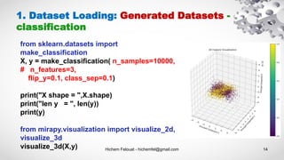
- 14. Hichem Felouat - hichemfel@gmail.com 14 1. Dataset Loading: Generated Datasets - classification from sklearn.datasets import make_classification X, y = make_classification( n_samples=10000, # n_features=3, flip_y=0.1, class_sep=0.1) print("X shape = ",X.shape) print("len y = ", len(y)) print(y) from mirapy.visualization import visualize_2d, visualize_3d visualize_3d(X,y)
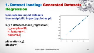
- 15. Hichem Felouat - hichemfel@gmail.com 15 1. Dataset loading: Generated Datasets - Regression from sklearn import datasets from matplotlib import pyplot as plt x, y = datasets.make_regression( n_samples=30, n_features=1, noise=0.8) plt.scatter(x,y) plt.show()
- 16. Hichem Felouat - hichemfel@gmail.com 16 1. Dataset Loading: Generated Datasets - Clustering from sklearn.datasets.samples_generator import make_blobs from matplotlib import pyplot as plt import pandas as pd X, y = make_blobs(n_samples=200, centers=4, n_features=2) Xy = pd.DataFrame(dict(x1=X[:,0], x2=X[:,1], label=y)) groups = Xy.groupby('label') fig, ax = plt.subplots() colors = ["blue", "red", "green", "purple"] for idx, classification in groups: classification.plot(ax=ax, kind='scatter', x='x1', y='x2', label=idx, color=colors[idx]) plt.show()
- 17. Hichem Felouat - hichemfel@gmail.com 17 2. Preprocessing Data: missing values Dealing with missing values : df = df.fillna('*') df[‘Test Score’] = df[‘Test Score’].fillna('*') df[‘Test Score’] = df[‘Test Score'].fillna(df['Test Score'].mean()) df['Test Score'] = df['Test Score'].fillna(df['Test Score'].interpolate()) df= df.dropna() #delete the missing rows of data df[‘Height(m)']= df[‘Height(m)’].dropna()
- 18. Hichem Felouat - hichemfel@gmail.com 18 2. Preprocessing Data: missing values # Dealing with Non-standard missing values: # dictionary of lists dictionary = {'Name’:[‘Alex’, ‘Mike’, ‘John’, ‘Dave’, ’Joey’], ‘Height(m)’: [1.75, 1.65, ‘-‘, ‘na’, 1.82], 'Test Score':[70, np.nan, 8, 62, 73]} # creating a dataframe from list df = pd.DataFrame(dictionary) df.isnull() df = df.replace(['-','na'], np.nan)
- 19. Hichem Felouat - hichemfel@gmail.com 19 2. Preprocessing Data: missing values import numpy as np from sklearn.impute import SimpleImputer X = [[np.nan, 2], [6, np.nan], [7, 6]] # mean, median, most_frequent, constant(fill_value = ) imp = SimpleImputer(missing_values = np.nan, strategy='mean') data = imp.fit_transform(X) print(data) Multivariate feature imputation : IterativeImputer Nearest neighbors imputation : KNNImputer Marking imputed values : MissingIndicator
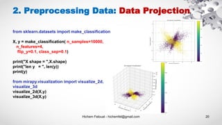
- 20. Hichem Felouat - hichemfel@gmail.com 20 2. Preprocessing Data: Data Projection from sklearn.datasets import make_classification X, y = make_classification( n_samples=10000, n_features=4, flip_y=0.1, class_sep=0.1) print("X shape = ",X.shape) print("len y = ", len(y)) print(y) from mirapy.visualization import visualize_2d, visualize_3d visualize_2d(X,y) visualize_3d(X,y)
- 21. Hichem Felouat - hichemfel@gmail.com 21 The sklearn.preprocessing package provides several common utility functions and transformer classes to change raw feature vectors into a representation that is more suitable for the downstream estimators. 1) Standardization 2) Non-linear transformation 3) Normalization 4) Encoding categorical features 5) Discretization 6) Generating polynomial features 7) Custom transformers 3. Feature Selection: Preprocessing
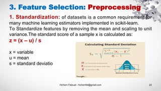
- 22. Hichem Felouat - hichemfel@gmail.com 22 3. Feature Selection: Preprocessing 1. Standardization: of datasets is a common requirement for many machine learning estimators implemented in scikit-learn. To Standardize features by removing the mean and scaling to unit variance.The standard score of a sample x is calculated as: z = (x – u) / s x = variable u = mean s = standard deviatio
- 23. Hichem Felouat - hichemfel@gmail.com 23 3. Feature Selection: 1. Standardization - StandardScaler from sklearn.preprocessing import StandardScaler import numpy as np X_train = np.array([[ 1., -1., 2.], [ 2., 0., 0.], [ 0., 1., -1.]]) scaler = StandardScaler().fit_transform(X_train) print(scaler) Out: [[ 0. -1.22474487 1.33630621] [ 1.22474487 0. -0.26726124] [-1.22474487 1.22474487 -1.06904497]]
- 24. Hichem Felouat - hichemfel@gmail.com 24 3. Feature Selection: 1. Standardization - Scaling Features to a Range import numpy as np from sklearn import preprocessing X_train = np.array([[ 1., -1., 2.], [ 2., 0., 0.], [ 0., 1., -1.]]) # Here is an example to scale a data matrix to the [0, 1] range: min_max_scaler = preprocessing.MinMaxScaler() X_train_minmax = min_max_scaler.fit_transform(X_train) print(X_train_minmax) # between a given minimum and maximum value min_max_scaler = preprocessing.MinMaxScaler(feature_range=(0, 10)) # scaling in a way that the training data lies within the range [-1, 1] max_abs_scaler = preprocessing.MaxAbsScaler()
- 25. Hichem Felouat - hichemfel@gmail.com 25 3. Feature Selection: 1. Standardization - Scaling Data with Outliers If your data contains many outliers, scaling using the mean and variance of the data is likely to not work very well. In these cases, you can use robust_scale and RobustScaler as drop-in replacements instead. They use more robust estimates for the center and range of your data. import numpy as np from sklearn import preprocessing X_train = np.array([[ 1., -1., 2.], [ 2., 0., 0.], [ 0., 1., -1.]]) scaler = preprocessing.RobustScaler() X_train_rob_scal = scaler.fit_transform(X_train) print(X_train_rob_scal)
- 26. Hichem Felouat - hichemfel@gmail.com 26 3. Feature Selection: 2. Non-linear Transformation - Mapping to a Uniform Distribution QuantileTransformer and quantile_transform provide a non-parametric transformation to map the data to a uniform distribution with values between 0 and 1: from sklearn.datasets import load_iris from sklearn.model_selection import train_test_split from sklearn import preprocessing import numpy as np X, y = load_iris(return_X_y=True) X_train, X_test, y_train, y_test = train_test_split(X, y, random_state=0) print(X_train) quantile_transformer = preprocessing.QuantileTransformer(random_state=0) X_train_trans = quantile_transformer.fit_transform(X_train) print(X_train_trans) X_test_trans = quantile_transformer.transform(X_test) # Compute the q-th percentile of the data along the specified axis. np.percentile(X_train[:, 0], [0, 25, 50, 75, 100])
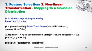
- 27. Hichem Felouat - hichemfel@gmail.com 27 3. Feature Selection: 2. Non-linear Transformation - Mapping to a Gaussian Distribution from sklearn import preprocessing import numpy as np pt = preprocessing.PowerTransformer(method='box-cox', standardize=False) X_lognormal = np.random.RandomState(616).lognormal(size=(3, 3)) print(X_lognormal) print(pt.fit_transform(X_lognormal))
- 28. Hichem Felouat - hichemfel@gmail.com 28 3. Feature Selection: 3. Normalization Normalization is the process of scaling individual samples to have unit norm. This process can be useful if you plan to use a quadratic form such as the dot-product or any other kernel to quantify the similarity of any pair of samples. from sklearn import preprocessing import numpy as np X = [[ 1., -1., 2.], [ 2., 0., 0.], [ 0., 1., -1.]] X_normalized = preprocessing.normalize(X, norm='l2') print(X_normalized)
- 29. Hichem Felouat - hichemfel@gmail.com 29 3. Feature Selection: 4. Encoding Categorical Features To convert categorical features to such integer codes, we can use the OrdinalEncoder. This estimator transforms each categorical feature to one new feature of integers (0 to n_categories - 1). from sklearn import preprocessing #genders = ['female', 'male'] #locations = ['from Africa', 'from Asia', 'from Europe', 'from US'] #browsers = ['uses Chrome', 'uses Firefox', 'uses IE', 'uses Safari'] X = [['male', 'from US', 'uses Safari'], ['female', 'from Europe', 'uses Safari'], ['female', 'from Asia', 'uses Firefox'], ['male', 'from Africa', 'uses Chrome']] enc = preprocessing.OrdinalEncoder() X_enc = enc.fit_transform(X) print(X_enc)
- 30. Hichem Felouat - hichemfel@gmail.com 30 3. Feature Selection: 5. Discretization Discretization (otherwise known as quantization or binning) provides a way to partition continuous features into discrete values.
- 31. Hichem Felouat - hichemfel@gmail.com 31 3. Feature Selection: 5. Discretization from sklearn import preprocessing import numpy as np X = np.array([[ -3., 5., 15 ], [ 0., 6., 14 ], [ 6., 3., 11 ]]) # 'onehot’, ‘onehot-dense’, ‘ordinal’ kbd = preprocessing.KBinsDiscretizer(n_bins=[3, 2, 2], encode='ordinal') X_kbd = kbd.fit_transform(X) print(X_kbd)
- 32. Hichem Felouat - hichemfel@gmail.com 32 3. Feature Selection: 5.1 Feature Binarization from sklearn import preprocessing import numpy as np X = [[ 1., -1., 2.],[ 2., 0., 0.],[ 0., 1., -1.]] binarizer = preprocessing.Binarizer() X_bin = binarizer.fit_transform(X) print(X_bin) # It is possible to adjust the threshold of the binarizer: binarizer_1 = preprocessing.Binarizer(threshold=1.1) X_bin_1 = binarizer_1.fit_transform(X) print(X_bin_1)
- 33. Hichem Felouat - hichemfel@gmail.com 33 3. Feature Selection: 6. Generating Polynomial Features Often it’s useful to add complexity to the model by considering nonlinear features of the input data. A simple and common method to use is polynomial features, which can get features’ high-order and interaction terms. It is implemented in PolynomialFeatures. for 2 features :
- 34. Hichem Felouat - hichemfel@gmail.com 34 3. Feature Selection: 6. Generating Polynomial Features from sklearn import preprocessing import numpy as np X = np.arange(9).reshape(3, 3) print(X) poly = preprocessing.PolynomialFeatures(degree=3, interaction_only=True) X_poly = poly.fit_transform(X) print(X_poly)
- 35. Hichem Felouat - hichemfel@gmail.com 35 3. Feature Selection: 7. Custom Transformers Often, you will want to convert an existing Python function into a transformer to assist in data cleaning or processing. You can implement a transformer from an arbitrary function with FunctionTransformer. For example, to build a transformer that applies a log transformation in a pipeline, do: from sklearn import preprocessing import numpy as np transformer = preprocessing.FunctionTransformer(np.log1p, validate=True) X = np.array([[0, 1], [2, 3]]) X_tr = transformer.fit_transform(X) print(X_tr)
- 36. Hichem Felouat - hichemfel@gmail.com 36 3. Feature Selection: Text Feature scikit-learn provides utilities for the most common ways to extract numerical features from text content, namely: • Tokenizing strings and giving an integer id for each possible token, for instance by using white-spaces and punctuation as token separators. • Counting the occurrences of tokens in each document. • Normalizing and weighting with diminishing importance tokens that occur in the majority of samples / documents.
- 37. Hichem Felouat - hichemfel@gmail.com 37 3. Feature Selection: Text Feature A simple way we can convert text to numeric feature is via binary encoding. In this scheme, we create a vocabulary by looking at each distinct word in the whole dataset (corpus). For each document, the output of this scheme will be a vector of size N where N is the total number of words in our vocabulary. Initially all entries in the vector will be 0. If the word in the given document exists in the vocabulary then vector element at that position is set to 1. CountVectorizer implements both tokenization and occurrence counting in a single class.
- 38. Hichem Felouat - hichemfel@gmail.com 38 from sklearn.feature_extraction.text import CountVectorizer texts = [ "blue car and blue window", "black crow in the window", "i see my reflection in the window" ] vec = CountVectorizer(binary=True) vec.fit(texts) print([w for w in sorted(vec.vocabulary_.keys())]) X = vec.transform(texts).toarray() print(X) import pandas as pd pd.DataFrame(vec.transform(texts).toarray(), columns=sorted(vec.vocabulary_.keys())) 3. Feature Selection: Text Feature
- 39. Hichem Felouat - hichemfel@gmail.com 39 bigram_vectorizer = CountVectorizer(ngram_range=(1, 2), token_pattern=r'bw+b', min_df=1) analyze = bigram_vectorizer.build_analyzer() analyze('Bi-grams are cool!') == ( ['bi', 'grams', 'are', 'cool', 'bi grams', 'grams are', 'are cool']) 3. Feature Selection: Text Feature To preserve some of the local ordering information we can extract 2-grams of words in addition to the 1-grams (individual words):
- 40. Hichem Felouat - hichemfel@gmail.com 40 3. Feature Selection: Text Feature Counting is another approach to represent text as a numeric feature. It is similar to Binary scheme that we saw earlier but instead of just checking if a word exists or not, it also checks how many times a word appeared. vec = CountVectorizer(binary=False)
- 41. Hichem Felouat - hichemfel@gmail.com 41 3. Feature Selection: Text Feature TF-IDF stands for term frequency-inverse document frequency. We saw that Counting approach assigns weights to the words based on their frequency and it’s obvious that frequently occurring words will have higher weights. But these words might not be important as other words. For example, let’s consider an article about Travel and another about Politics. Both of these articles will contain words like a, the frequently. But words such as flight, holiday will occur mostly in Travel and parliament, court etc. will appear mostly in Politics. Even though these words appear less frequently than the others, they are more important. TF-IDF assigns more weight to less frequently occurring words rather than frequently occurring ones. It is based on the assumption that less frequently occurring words are more important.
- 42. Hichem Felouat - hichemfel@gmail.com 42 3. Feature Selection: Text Feature from sklearn.feature_extraction.text import TfidfVectorizer texts = [ "blue car and blue window", "black crow in the window", "i see my reflection in the window" ] vec = TfidfVectorizer() vec.fit(texts) print([w for w in sorted(vec.vocabulary_.keys())]) X = vec.transform(texts).toarray() import pandas as pd pd.DataFrame(vec.transform(texts).toarray(), columns=sorted(vec.vocabulary_.keys()))
- 43. Hichem Felouat - hichemfel@gmail.com 43 3. Feature Selection: Image Feature #image.extract_patches_2d from sklearn.feature_extraction import image from sklearn.datasets import fetch_olivetti_faces import matplotlib.pyplot as plt import matplotlib.image as img data = fetch_olivetti_faces() plt.imshow(data.images[0]) patches = image.extract_patches_2d(data.images[0], (2, 2), max_patches=2,random_state=0) print('Image shape: {}'.format(data.images[0].shape),' Patches shape: {}'.format(patches.shape)) print('Patches = ',patches)
- 44. Hichem Felouat - hichemfel@gmail.com 44 3. Feature Selection: Image Feature import cv2 def hu_moments(image): image = cv2.cvtColor(image, cv2.COLOR_BGR2GRAY) feature = cv2.HuMoments(cv2.moments(image)).flatten() return feature def histogram(image,mask=None): image = cv2.cvtColor(image, cv2.COLOR_BGR2HSV) hist = cv2.calcHist([image],[0],None,[256],[0,256]) cv2.normalize(hist, hist) return hist.flatten()
- 45. Hichem Felouat - hichemfel@gmail.com 45 3. Feature Selection: Image Feature import mahotas def haralick_moments(image): #image = cv2.cvtColor(image, cv2.COLOR_BGR2GRAY) image = image.astype(int) haralick = mahotas.features.haralick(image).mean(axis=0) return haralick class ZernikeMoments: def __init__(self, radius): # store the size of the radius that will be # used when computing moments self.radius = radius def describe(self, image): # return the Zernike moments for the image return mahotas.features.zernike_moments(image, self.radius)
- 46. Hichem Felouat - hichemfel@gmail.com 46 3. Feature Selection: Image Feature from silx.opencl import sift sift_ocl = sift.SiftPlan(template=img, devicetype="GPU") keypoints = sift_ocl.keypoints(img)
- 47. Hichem Felouat - hichemfel@gmail.com 47 4. Dimensionality Reduction: Principal Component Analysis (PCA) Principal Component Analysis (PCA) is a statistical method that creates new features or characteristics of data by analyzing the characteristics of the dataset. Essentially, the characteristics of the data are summarized or combined together. You can also conceive of Principal Component Analysis as "squishing" data down into just a few dimensions from much higher dimensions space.
- 48. Hichem Felouat - hichemfel@gmail.com 48 from sklearn import datasets from sklearn.decomposition import PCA dat = datasets.load_breast_cancer() X, Y = dat.data, dat.target print("Examples = ",X.shape ," Labels = ", Y.shape) pca = PCA(n_components = 5) X_pca = pca.fit_transform(X) print("Examples = ",X_pca.shape ," Labels = ", Y.shape) 4. Dimensionality Reduction: Principal Component Analysis (PCA)
- 49. Hichem Felouat - hichemfel@gmail.com 49 4. Dimensionality Reduction: Kernel Principal Component Analysis (KPCA) Non-linear dimensionality reduction through the use of kernels. from sklearn import datasets from sklearn.decomposition import KernelPCA dat = datasets.load_breast_cancer() X, Y = dat.data, dat.target print("Examples = ",X.shape ," Labels = ", Y.shape) #kernel“linear” | “poly” | “rbf” | “sigmoid” | “cosine” | “precomputed” kpca = KernelPCA(n_components=7, kernel='rbf') X_kpca = kpca.fit_transform(X) print("Examples = ",X_kpca.shape ," Labels = ", Y.shape)
- 50. Hichem Felouat - hichemfel@gmail.com 50 4. Dimensionality Reduction: PCA VS KPCA
- 51. Hichem Felouat - hichemfel@gmail.com 51 4. Dimensionality Reduction: Linear Discriminant Analysis (LDA) In case of uniformly distributed data, LDA almost always performs better than PCA. However if the data is highly skewed (irregularly distributed) then it is advised to use PCA since LDA can be biased towards the majority class. from sklearn.discriminant_analysis import LinearDiscriminantAnalysis lda = LinearDiscriminantAnalysis(n_components=2) X_lda = lda.fit(X, Y).transform(X) print("Examples = ",X_lda.shape ," Labels = ", Y.shape)
- 52. Hichem Felouat - hichemfel@gmail.com 52 5. Training and Test Sets: Splitting Data from sklearn.model_selection import train_test_split from sklearn import datasets dat = datasets.load_iris() X = dat.data Y = dat.target print("Examples = ",X.shape ," Labels = ", Y.shape) # stratify : If not None, data is split in a stratified fashion, using this as the class labels. X_train, X_test, Y_train, Y_test = train_test_split(X, Y, test_size= 0.20, random_state=100, stratify=Y) print("X_train = ",X_train.shape ," Y_test = ", Y_test.shape)
- 53. Hichem Felouat - hichemfel@gmail.com 53 Supervised learning
- 54. Hichem Felouat - hichemfel@gmail.com 54 1. Regression: Linear regression Linear regression performs the task to predict a dependent variable value (y) based on a given independent variable (x). So, this regression technique finds out a linear relationship between x (input) and y (output). The equation of the above line is : Y= aX + b A regression model involving multiple variables can be represented as: Y = a1X1 + a2X2 + ... + anXn +b
- 55. Hichem Felouat - hichemfel@gmail.com 55 from sklearn.model_selection import train_test_split import matplotlib.pyplot as plt from mpl_toolkits.mplot3d import Axes3D from sklearn import datasets, linear_model from sklearn import metrics import numpy as np dat = datasets.load_boston() X = dat.data Y = dat.target print("Examples = ",X.shape ," Labels = ", Y.shape) fig, ax = plt.subplots(figsize=(12,8)) ax.scatter(X[:,0], Y, edgecolors=(0, 0, 0)) ax.plot([Y.min(), Y.max()], [Y.min(), Y.max()], 'k--', lw=4) ax.set_xlabel('F') ax.set_ylabel('Y') plt.show() fig = plt.figure(figsize=(12, 8)) ax = fig.add_subplot(111, projection='3d') ax.scatter(X[:, 0], X[:, 1], Y, c='b', marker='o',cmap=plt.cm.Set1, edgecolor='k', s=40) ax.set_title("My Data") ax.set_xlabel("F1") ax.w_xaxis.set_ticklabels([]) ax.set_ylabel("F2") ax.w_yaxis.set_ticklabels([]) ax.set_zlabel("Y") ax.w_zaxis.set_ticklabels([]) plt.show() X_train, X_test, Y_train, Y_test = train_test_split(X, Y, test_size= 0.20, random_state=100) print("X_train = ",X_train.shape ," Y_test = ", Y_test.shape) regressor = linear_model.LinearRegression() regressor.fit(X_train, Y_train) predicted = regressor.predict(X_test) import pandas as pd df = pd.DataFrame({'Actual': Y_test.flatten(), 'Predicted': predicted.flatten()}) print(df) df1 = df.head(25) df1.plot(kind='bar',figsize=(12,8)) plt.grid(which='major', linestyle='-', linewidth='0.5', color='green') plt.grid(which='minor', linestyle=':', linewidth='0.5', color='black') plt.show() predicted_all = regressor.predict(X) fig, ax = plt.subplots(figsize=(12,8)) ax.scatter(X[:,0], Y, edgecolors=(0, 0, 1)) ax.scatter(X[:,0], predicted_all, edgecolors=(1, 0, 0)) ax.set_xlabel('Measured') ax.set_ylabel('Predicted') plt.show() fig = plt.figure(figsize=(12, 8)) ax = fig.add_subplot(111, projection='3d') ax.scatter(X[:, 0], X[:, 1], Y, c='b', marker='o',cmap=plt.cm.Set1, edgecolor='k', s=40) ax.scatter(X[:, 0], X[:, 1], predicted_all, c='r', marker='o',cmap=plt.cm.Set1, edgecolor='k', s=40) ax.set_title("My Data") ax.set_xlabel("F1") ax.w_xaxis.set_ticklabels([]) ax.set_ylabel("F2") ax.w_yaxis.set_ticklabels([]) ax.set_zlabel("Y") ax.w_zaxis.set_ticklabels([]) plt.show() print('Mean Absolute Error : ', metrics.mean_absolute_error(Y_test, predicted)) print('Mean Squared Error : ', metrics.mean_squared_error(Y_test, predicted)) print('Root Mean Squared Error: ', np.sqrt(metrics.mean_squared_error(Y_test, predicted)))
- 56. Hichem Felouat - hichemfel@gmail.com 56 1. Regression: Learning Curves def plot_learning_curves(model, X, y): from sklearn.metrics import mean_squared_error X_train, X_val, y_train, y_val = train_test_split(X, y, test_size=0.2) train_errors, val_errors = [], [] for m in range(1, len(X_train)): model.fit(X_train[:m], y_train[:m]) y_train_predict = model.predict(X_train[:m]) y_val_predict = model.predict(X_val) train_errors.append(mean_squared_error(y_train_predict, y_train[:m])) val_errors.append(mean_squared_error(y_val_predict, y_val)) fig, ax = plt.subplots(figsize=(12,8)) ax.plot(np.sqrt(train_errors), "r-+", linewidth=2, label="train") ax.plot(np.sqrt(val_errors), "b-", linewidth=3, label="val") ax.legend(loc='upper right', bbox_to_anchor=(0.5, 1.1),ncol=1, fancybox=True, shadow=True) ax.set_xlabel('Training set size') ax.set_ylabel('RMSE') plt.show()
- 57. Hichem Felouat - hichemfel@gmail.com 57 1. Regression: Ridge regression from sklearn import datasets, linear_model # Regularization strength; must be a positive float. Regularization improves the conditioning of the problem and reduces the variance of the estimates. Larger values specify stronger regularization. regressor = linear_model.Ridge(alpha=.5) regressor.fit(X_train, Y_train) predicted = regressor.predict(X_test) # Bayesian Ridge Regression regressor = linear_model.BayesianRidge() # Lasso regressor = linear_model.Lasso(alpha=0.1) Ridge regression addresses some of the problems of Ordinary Least Squares by imposing a penalty on the size of the coefficients.
- 58. Hichem Felouat - hichemfel@gmail.com 58 1. Regression: Kernel Ridge regression from sklearn.kernel_ridge import KernelRidge # kernel = [linear,polynomial,rbf] regressor = KernelRidge(kernel ='rbf', alpha=1.0) regressor.fit(X_train, Y_train) predicted = regressor.predict(X_test) In order to explore nonlinear relations of the regression problem
- 59. Hichem Felouat - hichemfel@gmail.com 59 1. Regression: Polynomial Regression How to use a linear model to fit nonlinear data ? A simple way to do this is to add powers of each feature as new features, then train a linear model on this extended set of features. This technique is called Polynomial Regression.
- 60. Hichem Felouat - hichemfel@gmail.com 60 1. Regression: Polynomial Regression # generate some nonlinear data import numpy as np m = 1000 X = 6 * np.random.rand(m, 1) - 3 Y = 0.5 * X**2 + X + 2 + np.random.randn(m, 1) print("Examples = ",X.shape ," Labels = ", Y.shape) import matplotlib.pyplot as plt from mpl_toolkits.mplot3d import Axes3D fig, ax = plt.subplots(figsize=(12,8)) ax.scatter(X[:,0], Y, edgecolors=(0, 0, 1)) ax.set_xlabel('F') ax.set_ylabel('Y') plt.show() from sklearn.preprocessing import PolynomialFeatures poly_features = PolynomialFeatures(degree=2, include_bias=False) X_poly = poly_features.fit_transform(X) print("Examples = ",X_poly.shape ," Labels = ", Y.shape) from sklearn.model_selection import train_test_split X_train, X_test, Y_train, Y_test = train_test_split(X_poly, Y, test_size= 0.20, random_state=100) from sklearn import linear_model regressor = linear_model.LinearRegression() regressor.fit(X_train, Y_train) predicted = regressor.predict(X_poly) fig, ax = plt.subplots(figsize=(12,8)) ax.scatter(X, Y, edgecolors=(0, 0, 1)) ax.scatter(X,predicted,edgecolors=(1, 0, 0)) ax.set_xlabel('F') ax.set_ylabel('Y') plt.show() B = regressor.intercept_ A = regressor.coef_ print(A) print(B) print("The model estimates : Y = ",B[0]," + ",A[0,0]," X + ",A[0,1]," X^2") from sklearn import metrics predicted = regressor.predict(X_test) print('Mean Absolute Error : ', metrics.mean_absolute_error(Y_test, predicted)) print('Mean Squared Error : ', metrics.mean_squared_error(Y_test, predicted)) print('Root Mean Squared Error: ', np.sqrt(metrics.mean_squared_error(Y_test, predicted)))
- 61. Hichem Felouat - hichemfel@gmail.com 61 1. Regression: Support Vector Regression SVR The Support Vector Regression (SVR) uses the same principles as the SVM for classification, with only a few minor differences. from sklearn.svm import SVR svr_rbf = SVR(kernel='rbf', C=100, gamma=0.1, epsilon=.1) svr_lin = SVR(kernel='linear', C=100, gamma='auto') svr_poly = SVR(kernel='poly', C=100, gamma='auto', degree=3, epsilon=.1, coef0=1)
- 62. Hichem Felouat - hichemfel@gmail.com 62 1. Regression: Support Vector Regression SVR import numpy as np from sklearn.svm import SVR import matplotlib.pyplot as plt # Generate sample data X = np.sort(5 * np.random.rand(40, 1), axis=0) Y = np.sin(X).ravel() # Add noise to targets Y[::5] += 3 * (0.5 - np.random.rand(8)) print("Examples = ",X.shape ," Y = ", Y.shape) # Fit regression model svr_rbf = SVR(kernel='rbf', C=100, gamma=0.1, epsilon=.1) svr_lin = SVR(kernel='linear', C=100, gamma='auto') svr_poly = SVR(kernel='poly', C=100, gamma='auto', degree=3, epsilon=.1, coef0=1) # Look at the results lw = 2 svrs = [svr_rbf, svr_lin, svr_poly] kernel_label = ['RBF', 'Linear', 'Polynomial'] model_color = ['m', 'c', 'g'] fig, axes = plt.subplots(nrows=1, ncols=3, figsize=(15, 10), sharey=True) for ix, svr in enumerate(svrs): axes[ix].plot(X, svr.fit(X, Y).predict(X), color=model_color[ix], lw=lw, label='{} model'.format(kernel_label[ix])) axes[ix].scatter(X[svr.support_], Y[svr.support_], facecolor="none", edgecolor=model_color[ix], s=50, label='{} support vectors'.format(kernel_label[ix])) axes[ix].scatter(X[np.setdiff1d(np.arange(len(X)), svr.support_)], Y[np.setdiff1d(np.arange(len(X)), svr.support_)], facecolor="none", edgecolor="k", s=50, label='other training data') axes[ix].legend(loc='upper center', bbox_to_anchor=(0.5, 1.1), ncol=1, fancybox=True, shadow=True) fig.text(0.5, 0.04, 'data', ha='center', va='center') fig.text(0.06, 0.5, 'target', ha='center', va='center', rotation='vertical') fig.suptitle("Support Vector Regression", fontsize=14) plt.show()
- 63. Hichem Felouat - hichemfel@gmail.com 63 1. Regression: Decision Trees Regression
- 64. Hichem Felouat - hichemfel@gmail.com 64 1. Regression: Decision Trees Regression import matplotlib.pyplot as plt import numpy as np from sklearn.tree import DecisionTreeRegressor rng = np.random.RandomState(1) X = np.sort(5 * rng.rand(80, 1), axis=0) Y = np.sin(X).ravel() Y[::5] += 3 * (0.5 - rng.rand(16)) print("Examples = ",X.shape ," Labels = ", Y.shape) X_test = np.arange(0.0, 5.0, 0.01)[:, np.newaxis] regressor1 = DecisionTreeRegressor(max_depth=2) regressor2 = DecisionTreeRegressor(max_depth=5) regressor1.fit(X, Y) regressor2.fit(X, Y) predicted1 = regressor1.predict(X_test) predicted2 = regressor2.predict(X_test) plt.figure(figsize=(12,8)) plt.scatter(X, Y, s=20, edgecolor="black",c="darkorange", label="data") plt.plot(X_test, predicted1, color="cornflowerblue",label="max_depth=2", linewidth=2) plt.plot(X_test, predicted2, color="yellowgreen", label="max_depth=5", linewidth=2) plt.xlabel("data") plt.ylabel("target") plt.title("Decision Tree Regression") plt.legend() plt.show()
- 65. Hichem Felouat - hichemfel@gmail.com 65 1. Regression: Random Forest Regressor from sklearn.ensemble import RandomForestRegressor regressor = RandomForestRegressor(max_depth=5, random_state=0) regressor.fit(X, Y) predicted = regressor1.predict(X)
- 66. Hichem Felouat - hichemfel@gmail.com 66 2. Classification: Support Vector Machines The objective is to select a hyperplane with the maximum possible margin between support vectors in the given dataset. SVM searches for the maximum marginal hyperplane in the following steps: 1) Generate hyperplanes that separate the classes in the best way. Left-hand side figure showing three hyperplanes black, blue and orange. Here, the blue and orange have higher classification errors, but the black is separating the two classes correctly. 2) Select the right hyperplane with the maximum separation from either nearest data points as shown in the right-hand side figure.
- 67. Hichem Felouat - hichemfel@gmail.com 67 2. Classification: Support Vector Machines - Kernel Some problems can’t be solved using linear hyperplane, as shown in the figure below (left-hand side). In such situation, SVM uses a kernel to transform the input space to a higher dimensional space as shown on the right ( z=x^2 + y^2).
- 68. Hichem Felouat - hichemfel@gmail.com 68 2. Classification: Support Vector Machines - Kernel + Tuning Hyperparameters Regularization: Regularization: The C parameter controls how much you want to punish your model for each misclassified point for a given curve: Large values of C (Large effect of noisy points. A plane with very few misclassifications will be given precedence.). Small Values of C (Low effect of noisy points. Planes that separate the points well will be found, even if there are some misclassifications). Gamma (Kernel coefficient for rbf, poly and sigmoid): the low value of gamma considers only nearby points in calculating the separation line, while a high value of gamma considers all the data points in the calculation of the separation line.
- 69. Hichem Felouat - hichemfel@gmail.com 69 2. Classification: Support Vector Machines -Kernel + Tuning Hyperparameters from sklearn.svm import SVC # linear kernel svc_cls = SVC(kernel='linear') # Polynomial Kernel svc_cls = SVC(kernel='poly', degree=5, C=10, gamma=0.1) # Gaussian Kernel svc_cls = SVC(kernel='rbf', C=10, gamma=0.1) # Sigmoid Kernel svc_cls = SVC(kernel='sigmoid', C=10, gamma=0.1) svc_cls.fit(X_train, y_train)
- 70. Hichem Felouat - hichemfel@gmail.com 70 2. Classification: Support Vector Machines -Kernel + Tuning Hyperparameters import matplotlib.pyplot as plt from sklearn import datasets, svm, metrics from sklearn.model_selection import train_test_split digits = datasets.load_digits() _, axes = plt.subplots(2, 4) images_and_labels = list(zip(digits.images, digits.target)) for ax, (image, label) in zip(axes[0, :], images_and_labels[:4]): ax.set_axis_off() ax.imshow(image, cmap=plt.cm.gray_r, interpolation='nearest') ax.set_title('Training: %i' % label) # To apply a classifier on this data, we need to flatten the image, to # turn the data in a (samples, feature) matrix: n_samples = len(digits.images) data = digits.images.reshape((n_samples, -1)) # Create a classifier: a support vector classifier classifier = svm.SVC(gamma=0.001) # Split data into train and test subsets X_train, X_test, y_train, y_test = train_test_split( data, digits.target, test_size=0.5, shuffle=False) # We learn the digits on the first half of the digits classifier.fit(X_train, y_train) # Now predict the value of the digit on the second half: predicted = classifier.predict(X_test) images_and_predictions = list(zip(digits.images[n_samples // 2:], predicted)) for ax, (image, prediction) in zip(axes[1, :], images_and_predictions[:4]): ax.set_axis_off() ax.imshow(image, cmap=plt.cm.gray_r, interpolation='nearest') ax.set_title('Prediction: %i' % prediction) print("Classification report : n", classifier,"n", metrics.classification_report(y_test, predicted)) disp = metrics.plot_confusion_matrix(classifier, X_test, y_test) disp.figure_.suptitle("Confusion Matrix") print("Confusion matrix: n", disp.confusion_matrix) plt.show()
- 71. Hichem Felouat - hichemfel@gmail.com 71 2. Classification: Logistic Regression Classifier Logistic regression classifier: is a fundamental classification technique. It belongs to the group of linear classifiers and is somewhat similar to polynomial and linear regression. Logistic regression is fast and relatively uncomplicated, and it’s convenient for you to interpret the results. Although it’s essentially a method for binary classification, it can also be applied to multiclass problems. Your goal is to find the logistic regression function ( ) such that the predicted responses ( ) are as close as possible to the actual response for each observation = 1, …, . Sigmoid Function :
- 72. Hichem Felouat - hichemfel@gmail.com 72 from sklearn import datasets, metrics from sklearn.model_selection import train_test_split from sklearn.linear_model import LogisticRegression from sklearn.metrics import accuracy_score import matplotlib.pyplot as plt dat = datasets.load_breast_cancer() print("Examples = ",dat.data.shape ," Labels = ", dat.target.shape) X_train, X_test, Y_train, Y_test = train_test_split(dat.data, dat.target, test_size= 0.20, random_state=100) # default = ’auto’ logreg = LogisticRegression() logreg.fit(X_train,Y_train) predicted = logreg.predict(X_test) print("Classification report for classifier : n", metrics.classification_report(Y_test, predicted)) disp = metrics.plot_confusion_matrix(logreg, X_test, Y_test) disp.figure_.suptitle("Confusion Matrix") print("Confusion matrix: n", disp.confusion_matrix) plt.show() 2. Classification: Logistic Regression Classifier
- 73. Hichem Felouat - hichemfel@gmail.com 73 Advantages: Because of its efficient and straightforward nature, doesn't require high computation power, easy to implement, easily interpretable, used widely by data analyst and scientist. Also, it doesn't require scaling of features. Logistic regression provides a probability score for observations. Disadvantages: Logistic regression is not able to handle a large number of categorical features/variables. It is vulnerable to overfitting. Also, can't solve the non-linear problem with the logistic regression that is why it requires a transformation of non-linear features. Logistic regression will not perform well with independent variables that are not correlated to the target variable and are very similar or correlated to each other. 2. Classification: Logistic Regression Classifier
- 74. Hichem Felouat - hichemfel@gmail.com 74 2. Classification: Stochastic Gradient Descent Gradient Descent : at a theoretical level, gradient descent is an algorithm that minimizes functions. Given a function defined by a set of parameters, gradient descent starts with an initial set of parameter values and iteratively moves toward a set of parameter values that minimize the function. This iterative minimization is achieved using calculus, taking steps in the negative direction of the function gradient. Example: y = mx + b line equation where m is the line’s slope and b is the line’s y-intercept. To find the best line for our data, we need to find the best set of slope m and y- intercept b values. f(m,b): error function (also called a cost function) that measures how “good” a given line is. Each point in this two-dimensional space represents a line. The height of the function at each point is the error value for that line.
- 75. Hichem Felouat - hichemfel@gmail.com 75 Stochastic gradient descent (SGD): also known as incremental gradient descent, is an iterative method for optimizing a differentiable objective function, a stochastic approximation of gradient descent optimization. SGD has been successfully applied to large-scale and sparse machine learning problems often encountered in text classification and natural language processing. Given that the data is sparse, the classifiers in this module easily scale to problems with more than 10^5 training examples and more than 10^5 features. 2. Classification: Stochastic Gradient Descent
- 76. Hichem Felouat - hichemfel@gmail.com 76 2. Classification: Stochastic Gradient Descent from sklearn.linear_model import SGDClassifier X = [[0., 0.], [1., 1.]] y = [0, 1] # loss : hinge, log, modified_huber, squared_hinge, perceptron clf = SGDClassifier(loss="hinge", penalty="l2", max_iter=5) clf.fit(X, y) predicted = clf.predict(X_test)
- 77. Hichem Felouat - hichemfel@gmail.com 77 2. Classification: K-Nearest Neighbors KNN 1) Let's see this algorithm in action with the help of a simple example. Suppose you have a dataset with two variables, which when plotted, looks like the one in the following figure. 2) Your task is to classify a new data point with 'X' into "Blue" class or "Red" class. The coordinate values of the data point are x=45 and y=50. Suppose the value of K is 3. The KNN algorithm starts by calculating the distance of point X from all the points. It then finds the 3 nearest points with least distance to point X. This is shown in the figure below. The three nearest points have been encircled. 3) The final step of the KNN algorithm is to assign new point to the class to which majority of the three nearest points belong. From the figure above we can see that the two of the three nearest points belong to the class "Red" while one belongs to the class "Blue". Therefore the new data point will be classified as "Red".
- 78. Hichem Felouat - hichemfel@gmail.com 78 from sklearn.neighbors import KNeighborsClassifier from sklearn.model_selection import train_test_split from sklearn.datasets import load_iris from sklearn.metrics import classification_report, confusion_matrix import numpy as np import matplotlib.pyplot as plt # Loading data irisData = load_iris() # Create feature and target arrays X = irisData.data y = irisData.target # Split into training and test set X_train, X_test, y_train, y_test = train_test_split( X, y, test_size = 0.2, random_state=42) knn = KNeighborsClassifier(n_neighbors = 7) knn.fit(X_train, y_train) predicted = knn.predict(X_test) print(confusion_matrix(y_test, predicted)) print(classification_report(y_test, predicted)) 2. Classification: K-Nearest Neighbors KNN neighbors = np.arange(1, 25) train_accuracy = np.empty(len(neighbors)) test_accuracy = np.empty(len(neighbors)) # Loop over K values for i, k in enumerate(neighbors): knn = KNeighborsClassifier(n_neighbors=k) knn.fit(X_train, y_train) # Compute traning and test data accuracy train_accuracy[i] = knn.score(X_train, y_train) test_accuracy[i] = knn.score(X_test, y_test) # Generate plot plt.plot(neighbors, test_accuracy, label = 'Testing dataset Accuracy') plt.plot(neighbors, train_accuracy, label = 'Training dataset Accuracy') plt.legend() plt.xlabel('n_neighbors') plt.ylabel('Accuracy') plt.show()
- 79. Hichem Felouat - hichemfel@gmail.com 79 2. Classification: K-Nearest Neighbors KNN Advantages: 1) It is extremely easy to implement 2) Requires no training prior to making real time predictions. This makes the KNN algorithm much faster than other algorithms that require training e.g SVM, linear regression, etc. 3) New data can be added seamlessly. 4) There are only two parameters required to implement KNN i.e. the value of K and the distance function (e.g. Euclidean or Manhattan etc.) Disadvantages: 1) The KNN algorithm doesn't work well with high dimensional data because with large number of dimensions, it becomes difficult for the algorithm to calculate distance in each dimension. 2) The KNN algorithm has a high prediction cost for large datasets. This is because in large datasets the cost of calculating distance between new point and each existing point becomes higher. 3) Finally, the KNN algorithm doesn't work well with categorical features since it is difficult to find the distance between dimensions with categorical features.
- 80. Hichem Felouat - hichemfel@gmail.com 80 2. Classification: Naive Bayes Classification Naive Bayes: is a probabilistic machine learning algorithm that can be used in a wide variety of classification tasks. Typical applications include filtering spam, classifying documents, sentiment prediction, etc. It is based on the Bayes theory.
- 81. Hichem Felouat - hichemfel@gmail.com 81 2. Classification: Naive Bayes Classification The Bayes Rule provides the formula for the probability of Y given X. But, in real-world problems, you typically have multiple X variables. When the features are independent, we can extend the Bayes Rule to what is called Naive Bayes.
- 82. Hichem Felouat - hichemfel@gmail.com 82 2. Classification: Naive Bayes Classification Laplace Correction : when you have a model with many features if the entire probability will become zero because one of the feature’s value was zero. To avoid this, we increase the count of the variable with zero to a small value (usually 1) in the numerator, so that the overall probability doesn’t become zero. Since P(x1, x2, ... , xn) is constant given the input, we can use the following classification rule:
- 83. Hichem Felouat - hichemfel@gmail.com 83 2. Classification: Naive Bayes Classification weather Temperature Play 1 Sunny Hot No 2 Sunny Hot No 3 Overcast Hot Yes 4 Rainy Mild Yes 5 Rainy Cool Yes 6 Rainy Cool No 7 Overcast Cool Yes 8 Sunny Mild No 9 Sunny Cool Yes 10 Rainy Mild Yes 11 Sunny Mild Yes 12 Overcast Mild Yes 13 Overcast Hot No 14 Rainy Mild No weather No Yes P(No) P(Yes) Sunny 3 2 3/6 2/8 Overcast 1 3 1/6 3/8 Rainy 2 3 2/6 3/8 Total 6 8 6/14 8/14 Temperature No Yes P(No) P(Yes) Hot 3 1 3/6 1/8 Mild 2 4 2/6 4/8 cool 1 3 1/6 3/8 Total 6 8 6/14 8/14
- 84. Hichem Felouat - hichemfel@gmail.com 84 2. Classification: Naive Bayes Classification # Assigning features and label variables weather=['Sunny','Sunny','Overcast','Rainy','Rainy','R ainy','Overcast','Sunny','Sunny', 'Rainy','Sunny','Overcast','Overcast','Rainy'] temp=['Hot','Hot','Hot','Mild','Cool','Cool','Cool','Mild',' Cool','Mild','Mild','Mild','Hot','Mild'] play=['No','No','Yes','Yes','Yes','No','Yes','No','Yes','Ye s','Yes','Yes','No','No'] # Import LabelEncoder from sklearn import preprocessing # creating labelEncoder le = preprocessing.LabelEncoder() # Converting string labels into numbers. weather_encoded=le.fit_transform(weather) print("weather:",wheather_encoded) # Converting string labels into numbers temp_encoded=le.fit_transform(temp) label=le.fit_transform(play) print("Temp: ",temp_encoded) print("Play: ",label) # Combinig weather and temp into single listof tuples features = zip(weather_encoded,temp_encoded) import numpy as np features = np.asarray(list(features)) print("features : ",features) #Import Gaussian Naive Bayes model from sklearn.naive_bayes import GaussianNB #Create a Gaussian Classifier model = GaussianNB() # Train the model using the training sets model.fit(features,label) # Predict Output predicted= model.predict([[0,2]]) # 0:Overcast, 2:Mild print ("Predicted Value (No = 0, Yes = 1):", predicted)
- 85. Hichem Felouat - hichemfel@gmail.com 85 2. Classification: Gaussian Naive Bayes Classification In Gaussian Naive Bayes, continuous values associated with each feature are assumed to be distributed according to a Gaussian distribution. A Gaussian distribution is also called Normal distribution. The likelihood of the features is assumed to be Gaussian, hence, conditional probability is given by:
- 86. Hichem Felouat - hichemfel@gmail.com 86 2. Classification: Gaussian Naive Bayes Classification # load the iris dataset from sklearn.datasets import load_iris iris = load_iris() # store the feature matrix (X) and response vector (y) X = iris.data y = iris.target # splitting X and y into training and testing sets from sklearn.model_selection import train_test_split X_train, X_test, y_train, y_test = train_test_split(X, y, test_size=0.4, random_state=100) # training the model on training set from sklearn.naive_bayes import GaussianNB gnb = GaussianNB() gnb.fit(X_train, y_train) # making predictions on the testing set y_pred = gnb.predict(X_test) # comparing actual response values (y_test) with predicted response values (y_pred) from sklearn import metrics print("Gaussian Naive Bayes model accuracy(in %):", metrics.accuracy_score(y_test, y_pred)*100) print("Number of mislabeled points out of a total %d points : %d" % (X_test.shape[0], (y_test != y_pred).sum()))
- 87. Hichem Felouat - hichemfel@gmail.com 87 2. Classification: Multinomial Naive Bayes Classification In multinomial naive Bayes, the features are assumed to be generated from a simple multinomial distribution. The multinomial distribution describes the probability of observing counts among a number of categories, and thus multinomial naive Bayes is most appropriate for features that represent counts or count rates. Advantages: 1) They are extremely fast for both training and prediction. 2) They provide a straightforward probabilistic prediction. 3) They are often very easily interpretable. 4) They have very few (if any) tunable parameters.
- 88. Hichem Felouat - hichemfel@gmail.com 88 2. Classification: Multinomial Naive Bayes Classification from sklearn.datasets import fetch_20newsgroups data = fetch_20newsgroups() print(data.target_names) # For simplicity here, we will select just a few of these categories categories = ['talk.religion.misc', 'soc.religion.christian', 'sci.space', 'comp.graphics'] sub_data = fetch_20newsgroups(subset='train', categories=categories) X, Y = sub_data.data, sub_data.target print("Examples = ",len(X)," Labels = ", len(Y)) # Here is a representative entry from the data: print(X[5]) # In order to use this data for machine learning, we need to be able to convert the content of each string into a vector of numbers. # For this we will use the TF-IDF vectorizer from sklearn.feature_extraction.text import TfidfVectorizer vec = TfidfVectorizer() vec.fit(X) texts = vec.transform(X).toarray() print(" texts shape = ",texts.shape) # split the dataset into training data and test data from sklearn.model_selection import train_test_split X_train, X_test, Y_train, Y_test = train_test_split(texts, Y, test_size= 0.20, random_state=100, stratify=Y) # training the model on training set from sklearn.naive_bayes import MultinomialNB clf = MultinomialNB() clf.fit(X_train, Y_train) # making predictions on the testing set predicted = clf.predict(X_test) from sklearn import metrics print("Classification report : n", clf,"n", metrics.classification_report(Y_test, predicted)) disp = metrics.plot_confusion_matrix(clf, X_test, Y_test) disp.figure_.suptitle("Confusion Matrix") print("Confusion matrix: n", disp.confusion_matrix)
- 89. Hichem Felouat - hichemfel@gmail.com 89 2. Classification: Decision Trees Decision trees are supervised learning algorithms used for both, classification and regression tasks. The main idea of decision trees is to find the best descriptive features which contain the most information regarding the target feature and then split the dataset along the values of these features such that the target feature values for the resulting sub_datasets are as pure as possible. The descriptive feature which leaves the target feature most purely is said to be the most informative one. This process of finding the most informative feature is done until we accomplish a stopping criterion where we then finally end up in so-called leaf nodes. The leaf nodes contain the predictions we will make for new query instances presented to our trained model. This is possible since the model has kind of learned the underlying structure of the training data and hence can, given some assumptions, make predictions about the target feature value (class) of unseen query instances.
- 90. Hichem Felouat - hichemfel@gmail.com 90 2. Classification: Decision Trees
- 91. Hichem Felouat - hichemfel@gmail.com 91 2. Classification: Decision Trees How does the Decision Tree algorithm work? Attribute selection measure (ASM): is a heuristic for selecting the splitting criterion that partition data into the best possible manner. 1) Select a test for root node. Create branch for each possible outcome of the test. 2) Split instances into subsets. One for each branch extending from the node. 3) Repeat recursively for each branch, using only instances that reach the branch. 4) Stop recursion for a branch if all its instances have the same class.
- 92. Hichem Felouat - hichemfel@gmail.com 92 2. Classification: Decision Trees
- 93. Hichem Felouat - hichemfel@gmail.com 93 2. Classification: Decision Trees - Example from sklearn.datasets import load_iris from sklearn.tree import DecisionTreeClassifier # load the iris dataset dat = load_iris() # store the feature matrix (X) and response vector (y) X = dat.data y = dat.target # splitting X and y into training and testing sets from sklearn.model_selection import train_test_split X_train, X_test, y_train, y_test = train_test_split(X, y, test_size=0.2, random_state=100) # training the model on training set # criterion='gini' splitter='best' max_depth=2 tree_clf = DecisionTreeClassifier(max_depth=2) tree_clf.fit(X_train, y_train) # making predictions on the testing set predicted = tree_clf.predict(X_test) # comparing actual response values (y_test) with predicted response values (predicted) from sklearn import metrics print("Classification report : n", tree_clf,"n", metrics.classification_report(y_test, predicted)) disp = metrics.plot_confusion_matrix(tree_clf, X_test, y_test) disp.figure_.suptitle("Confusion Matrix") print("Confusion matrix: n", disp.confusion_matrix) # plot the tree with the plot_tree function: from sklearn import tree tree.plot_tree(tree_clf.fit(X_train, y_train))
- 94. Hichem Felouat - hichemfel@gmail.com 94 2. Classification: Decision Trees - Example # Visualize data import collections import pydotplus dot_data = tree.export_graphviz(tree_clf, feature_names=dat.feature_names, out_file=None, filled=True, rounded=True) graph = pydotplus.graph_from_dot_data(dot_data) colors = ('turquoise', 'orange') edges = collections.defaultdict(list) for edge in graph.get_edge_list(): edges[edge.get_source()].append(int(edge.get_destination())) for edge in edges: edges[edge].sort() for i in range(2): dest = graph.get_node(str(edges[edge][i]))[0] dest.set_fillcolor(colors[i]) graph.write_png('tree1.png') #pdf import graphviz dot_data = tree.export_graphviz(tree_clf, out_file=None) graph = graphviz.Source(dot_data) graph.render("iris") dot_data = tree.export_graphviz(tree_clf, out_file=None, feature_names=dat.feature_names, class_names=dat.target_names, filled=True, rounded=True, special_characters=True) graph = graphviz.Source(dot_data) graph.view('tree2.pdf')
- 95. Hichem Felouat - hichemfel@gmail.com 95 2. Classification: Decision Trees - Example
- 96. Hichem Felouat - hichemfel@gmail.com 96 Gini impurity: 2. Classification: Decision Trees Entropy:
- 97. Hichem Felouat - hichemfel@gmail.com 97 Estimating Class Probabilities: A Decision Tree can also estimate the probability that an instance belongs to a particular class k: first it traverses the tree to find the leaf node for this instance, and then it returns the ratio of training instances of class k in this node. 2. Classification: Decision Trees print("predict_proba : ",tree_clf.predict_proba([[1, 1.5, 3.2, 0.5]])) predict_proba : [[0. 0.91489362 0.08510638]] Scikit-Learn uses the CART algorithm, which produces only binary trees: nonleaf nodes always have two children (i.e., questions only have yes/no answers). However, other algorithms such as ID3 can produce Decision Trees with nodes that have more than two children.
- 98. Hichem Felouat - hichemfel@gmail.com 98 2. Classification: Random Forest Classifier The random forest classifier is a supervised learning algorithm and composed of multiple decision trees. By averaging out the impact of several decision trees, random forests tend to improve prediction. 1) Select random samples from a given dataset. 2) Construct a decision tree for each sample and get a prediction result from each decision tree. 3) Perform a vote for each predicted result. 4) Select the prediction result with the most votes as the final prediction,
- 99. Hichem Felouat - hichemfel@gmail.com 99 2. Classification: Random Forest Classifier Advantages: 1) Random forests is considered as a highly accurate and robust method because of the number of decision trees participating in the process. 2) It does not suffer from the overfitting problem. The main reason is that it takes the average of all the predictions, which cancels out the biases. 3) The algorithm can be used in both classification and regression problems. Disadvantages: 1) Random forests is slow in generating predictions because it has multiple decision trees. Whenever it makes a prediction, all the trees in the forest have to make a prediction for the same given input and then perform voting on it. This whole process is time-consuming. 2) The model is difficult to interpret compared to a decision tree, where you can easily make a decision by following the path in the tree.
- 100. Hichem Felouat - hichemfel@gmail.com 100 2. Classification: Random Forest Classifier # Import scikit-learn dataset library from sklearn import datasets # Load dataset dat = datasets.load_iris() X = dat.data y = dat.target # Split dataset into training set and test set 70% training and 30% test from sklearn.model_selection import train_test_split X_train, X_test, y_train, y_test = train_test_split(X, y, test_size=0.3, random_state=100) # training the model on training set from sklearn.ensemble import RandomForestClassifier # n_estimators : The number of trees in the forest. # max_depth : The maximum depth of the tree. # n_jobsint : The number of jobs to run in parallel rf_clf = RandomForestClassifier(n_estimators=10) rf_clf.fit(X_train,y_train) # making predictions on the testing set predicted = rf_clf.predict(X_test) # comparing actual response values (y_test) with predicted response values (predicted) from sklearn import metrics print("Classification report : n", rf_clf,"n", metrics.classification_report(y_test, predicted)) disp = metrics.plot_confusion_matrix(rf_clf, X_test, y_test) disp.figure_.suptitle("Confusion Matrix") print("Confusion matrix: n", disp.confusion_matrix)
- 101. Hichem Felouat - hichemfel@gmail.com 101 3. Ensemble Methods The goal of ensemble methods is to combine the predictions of several base estimators built with a given learning algorithm in order to improve generalizability / robustness over a single estimator. Two families of ensemble methods are usually distinguished: In averaging methods, the driving principle is to build several estimators independently and then to average their predictions. On average, the combined estimator is usually better than any of the single base estimator because its variance is reduced. Examples: Bagging methods, Forests of randomized trees, … By contrast, in boosting methods, base estimators are built sequentially and one tries to reduce the bias of the combined estimator. The motivation is to combine several weak models to produce a powerful ensemble. Examples: AdaBoost, Gradient Tree Boosting, …
- 102. Hichem Felouat - hichemfel@gmail.com 102 3. Ensemble Methods: Voting Classifier The idea behind the VotingClassifier is to combine conceptually different machine learning classifiers and use a majority vote (Hard Voting) or the average predicted probabilities (soft vote) to predict the class labels. Such a classifier can be useful for a set of equally well performing model in order to balance out their individual weaknesses. Ensemble methods work best when the predictors are as independent from one another as possible. One way to get diverse classifiers is to train them using very different algorithms. This increases the chance that they will make very different types of errors, improving the ensemble’s accuracy.
- 103. Hichem Felouat - hichemfel@gmail.com 103 from sklearn import datasets from sklearn.model_selection import train_test_split from sklearn.ensemble import RandomForestClassifier, VotingClassifier from sklearn.linear_model import LogisticRegression from sklearn.svm import SVC from sklearn.metrics import accuracy_score dat = datasets.load_breast_cancer() print("Examples = ",dat.data.shape ," Labels = ", dat.target.shape) X_train, X_test, Y_train, Y_test = train_test_split(dat.data, dat.target, test_size= 0.20, random_state=100) log_clf = LogisticRegression() rnd_clf = RandomForestClassifier() svm_clf = SVC() voting_clf = VotingClassifier( estimators=[('lr', log_clf), ('rf', rnd_clf), ('svc', svm_clf)],voting='hard') voting_clf.fit(X_train, Y_train) for clf in (log_clf, rnd_clf, svm_clf, voting_clf): clf.fit(X_train, Y_train) y_pred = clf.predict(X_test) print(clf.__class__.__name__, accuracy_score(Y_test, y_pred)) 3. Ensemble Methods: Voting Classifier
- 104. Hichem Felouat - hichemfel@gmail.com 104 3. Ensemble Methods: Voting Classifier - (Soft Voting) Soft voting returns the class label as argmax of the sum of predicted probabilities. Specific weights can be assigned to each classifier via the weights parameter. When weights are provided, the predicted class probabilities for each classifier are collected, multiplied by the classifier weight, and averaged. The final class label is then derived from the class label with the highest average probability. Example: w1=1, w2=1, w3=1. Here, the predicted class label is 2, since it has the highest average probability.
- 105. Hichem Felouat - hichemfel@gmail.com 105 3. Ensemble Methods: Voting Classifier - (Soft Voting) from sklearn import datasets from sklearn.tree import DecisionTreeClassifier from sklearn.neighbors import KNeighborsClassifier from sklearn.svm import SVC from itertools import product from sklearn.ensemble import VotingClassifier from sklearn.model_selection import train_test_split # Loading some example data dat = datasets.load_iris() X_train, X_test, Y_train, Y_test = train_test_split(dat.data, dat.target, test_size= 0.20, random_state=100) # Training classifiers clf1 = DecisionTreeClassifier(max_depth=4) clf2 = KNeighborsClassifier(n_neighbors=7) clf3 = SVC(kernel='rbf', probability=True) voting_clf_soft = VotingClassifier(estimators=[('dt', clf1), ('knn', clf2), ('svc', clf3)], voting='soft', weights=[2, 1, 3]) for clf in (clf1, clf2, clf3, voting_clf_soft): clf.fit(X_train, Y_train) y_pred = clf.predict(X_test) print(clf.__class__.__name__, accuracy_score(Y_test, y_pred))
- 106. Hichem Felouat - hichemfel@gmail.com 106 from sklearn.datasets import load_boston from sklearn.ensemble import GradientBoostingRegressor, RandomForestRegressor,VotingRegressor from sklearn.linear_model import LinearRegression from sklearn.model_selection import train_test_split from sklearn import metrics import numpy as np # Loading some example data dat = load_boston() X_train, X_test, Y_train, Y_test = train_test_split(dat.data, dat.target, test_size= 0.20, random_state=100) # Training classifiers reg1 = GradientBoostingRegressor(random_state=1, n_estimators=10) reg2 = RandomForestRegressor(random_state=1, n_estimators=10) reg3 = LinearRegression() voting_reg = VotingRegressor(estimators=[('gb', reg1), ('rf', reg2), ('lr', reg3)], weights=[1, 3, 2]) for clf in (reg1, reg2, reg3, voting_reg): clf.fit(X_train, Y_train) y_pred = clf.predict(X_test) print(clf.__class__.__name__," : **********") print('Mean Absolute Error : ', metrics.mean_absolute_error(Y_test, y_pred)) print('Mean Squared Error : ', metrics.mean_squared_error(Y_test, y_pred)) print('Root Mean Squared Error: ', np.sqrt(metrics.mean_squared_error(Y_test, y_pred))) 3. Ensemble Methods: Voting Regressor
- 107. Hichem Felouat - hichemfel@gmail.com 107 3. Ensemble Methods: Bagging and Pasting In this approach, we use the same training algorithm for every predictor, but to train them on different random subsets of the training set. When sampling is performed with replacement, this method is called bagging (short for bootstrap aggregating). When sampling is performed without replacement, it is called pasting.
- 108. Hichem Felouat - hichemfel@gmail.com 108 from sklearn.ensemble import BaggingClassifier from sklearn.tree import DecisionTreeClassifier bag_clf = BaggingClassifier( DecisionTreeClassifier(), n_estimators=500, max_samples=100, bootstrap=True, n_jobs=-1) bag_clf.fit(X_train, y_train) y_pred = bag_clf.predict(X_test) 3. Ensemble Methods: Bagging and Pasting This is an example of bagging, but if you want to use pasting instead, just set bootstrap=False
- 109. Hichem Felouat - hichemfel@gmail.com 109 3. Ensemble Methods: AdaBoost The technique used by AdaBoost is the new predictor correcting its predecessor. For example, to build an AdaBoost classifier, a first base classifier (such as a Decision Tree) is trained and used to make predictions on the training set. The relative weight of misclassified training instances is then increased. A second classifier is trained using the updated weights and again it makes predictions on the training set, weights are updated, and so on.
- 110. Hichem Felouat - hichemfel@gmail.com 110 3. Ensemble Methods: AdaBoost from sklearn.ensemble import AdaBoostClassifier from sklearn.datasets import load_iris from sklearn.model_selection import train_test_split from sklearn.tree import DecisionTreeClassifier X, y = load_iris(return_X_y=True) X_train, X_test, y_train, y_test = train_test_split(X, y, test_size= 0.20, random_state=100) ada_clf = AdaBoostClassifier( DecisionTreeClassifier(max_depth=1), n_estimators=100, algorithm="SAMME.R", learning_rate=0.5) ada_clf.fit(X_train, y_train) # making predictions on the testing set predicted = ada_clf.predict(X_test) # comparing actual response values (y_test) with predicted response values (predicted) from sklearn import metrics print("Classification report : n", ada_clf,"n", metrics.classification_report(y_test, predicted)) disp = metrics.plot_confusion_matrix(ada_clf, X_test, y_test) disp.figure_.suptitle("Confusion Matrix") print("Confusion matrix: n", disp.confusion_matrix)
- 111. Hichem Felouat - hichemfel@gmail.com 111 3. Ensemble Methods: Gradient Boosting Instead of adjusting the instance weights at every iteration as AdaBoost does, this method tries to fit the new predictor to the residual errors made by the previous predictor.
- 112. Hichem Felouat - hichemfel@gmail.com 112 3. Ensemble Methods: Gradient Boosting - Classification from sklearn import datasets # Load dataset dat = datasets.load_iris() X = dat.data y = dat.target # Split dataset into training set and test set 70% training and 30% test from sklearn.model_selection import train_test_split X_train, X_test, y_train, y_test = train_test_split(X, y, test_size=0.3, random_state=100) # training the model on training set from sklearn.ensemble import GradientBoostingClassifier clf = GradientBoostingClassifier(n_estimators=100, learning_rate=1.0, max_depth=1, random_state=0) clf.fit(X_train, y_train) # making predictions on the testing set predicted = clf.predict(X_test) # comparing actual response values (y_test) with predicted response values (predicted) from sklearn import metrics print("Classification report : n", clf,"n", metrics.classification_report(y_test, predicted)) disp = metrics.plot_confusion_matrix(clf, X_test, y_test) disp.figure_.suptitle("Confusion Matrix") print("Confusion matrix: n", disp.confusion_matrix)
- 113. Hichem Felouat - hichemfel@gmail.com 113 3. Ensemble Methods: Gradient Boosting - Regression from sklearn.datasets import load_boston from sklearn.model_selection import train_test_split from sklearn import metrics import numpy as np # Loading some example data dat = load_boston() X_train, X_test, y_train, y_test = train_test_split(dat.data, dat.target, test_size= 0.20, random_state=100) # Training classifiers from sklearn.ensemble import GradientBoostingRegressor clf = GradientBoostingRegressor(n_estimators=100, learning_rate=0.1, max_depth=1, random_state=0, loss='ls') clf.fit(X_train, y_train) y_pred = clf.predict(X_test) print('Mean Absolute Error : ', metrics.mean_absolute_error(Y_test, y_pred)) print('Mean Squared Error : ', metrics.mean_squared_error(Y_test, y_pred)) print('Root Mean Squared Error: ', np.sqrt(metrics.mean_squared_error(Y_test, y_pred)))
- 114. Hichem Felouat - hichemfel@gmail.com 114 3. Ensemble Methods: XGBoost XGBoost is a specific implementation of the Gradient Boosting method which uses more accurate approximations to find the best tree model. It employs a number of nifty tricks that make it exceptionally successful, particularly with structured data. XGBoost is often an important component of the winning entries in ML competitions.
- 115. Hichem Felouat - hichemfel@gmail.com 115 3. Ensemble Methods: XGBoost - Classification from sklearn.datasets import load_iris from sklearn.model_selection import train_test_split X, y = load_iris(return_X_y=True) X_train, X_test, y_train, y_test = train_test_split(X, y, test_size= 0.20, random_state=100) # In order for XGBoost to be able to use our data, # we’ll need to transform it into a specific format that XGBoost can handle. D_train = xgb.DMatrix(X_train, label=y_train) D_test = xgb.DMatrix(X_test, label=y_test) # Training classsifier import xgboost as xgb param = {'eta': 0.3, 'max_depth': 3, 'objective': 'multi:softprob', 'num_class': 3} steps = 20 # The number of training iterations xg_clf = xgb.train(param, D_train, steps) # making predictions on the testing set predicted = xg_reg.predict(X_test) # comparing actual response values (y_test) with predicted response values (predicted) from sklearn import metrics print("Classification report : n", xg_clf,"n", metrics.classification_report(y_test, predicted)) disp.figure_.suptitle("Confusion Matrix") print("Confusion matrix: n", disp.confusion_matrix) # Visualize Boosting Trees and # Feature Importance import matplotlib.pyplot as plt xgb.plot_tree(xg_clf,num_trees=0) plt.rcParams['figure.figsize'] = [10, 10] plt.show() xgb.plot_importance(xg_clf) plt.rcParams['figure.figsize'] = [5, 5] plt.show()
- 116. Hichem Felouat - hichemfel@gmail.com 116 3. Ensemble Methods: XGBoost - Regression import xgboost as xgb xg_reg = xgb.XGBRegressor(objective ='reg:linear', colsample_bytree = 0.3, learning_rate = 0.1, max_depth = 5, alpha = 10, n_estimators = 10) xg_reg.fit(X_train,y_train) predicted = xg_reg.predict(X_test)
- 117. Hichem Felouat - hichemfel@gmail.com 117 4. Cross-Validation Cross-Validation (CV) : the training set is split into complementary subsets, and each model is trained against a different combination of these subsets and validated against the remaining parts. Once the model type and hyperparameters have been selected, a final model is trained using these hyperparameters on the full training set, and the generalized error is measured on the test set.
- 118. Hichem Felouat - hichemfel@gmail.com 118 4. Cross-Validation
- 119. Hichem Felouat - hichemfel@gmail.com 119 4. Cross-Validation k-fold cross-validation, the data is divided into k folds. The model is trained on k-1 folds with one fold held back for testing. This process gets repeated to ensure each fold of the dataset gets the chance to be the held backset. Once the process is completed, we can summarize the evaluation metric using the mean or/and the standard deviation. Stratified K-Fold approach is a variation of k-fold cross-validation that returns stratified folds, i.e., each set containing approximately the same ratio of target labels as the complete data.
- 120. Hichem Felouat - hichemfel@gmail.com 120 4. Cross-Validation Leave One Out Cross-Validation (LOOCV) is the cross-validation technique in which the size of the fold is “1” with “k” being set to the number of observations in the data. This variation is useful when the training data is of limited size and the number of parameters to be tested is not high. Repeated Random Test-Train Splits is a hybrid of traditional train-test splitting and the k-fold cross-validation method. In this technique, we create random splits of the data in the training-test set manner and then repeat the process of splitting and evaluating the algorithm multiple times, just like the cross-validation method.
- 121. Hichem Felouat - hichemfel@gmail.com 121 4. Cross-Validation import numpy as np from sklearn import datasets from sklearn.model_selection import train_test_split from sklearn import svm from sklearn.model_selection import cross_val_score from sklearn import model_selection from sklearn import metrics dat = datasets.load_breast_cancer() print("Examples = ",dat.data.shape ," Labels = ", dat.target.shape) print("Example 0 = ",dat.data[0]) print("Label 0 =",dat.target[0]) print(dat.target) X = dat.data Y = dat.target # Make a train/test split using 20% test size X_train, X_test, Y_train, Y_test = train_test_split(X, Y, test_size= 0.20, random_state=100) print("X_test = ",X_test.shape) print("Without Validation : *********") model_1 = svm.SVC(kernel='linear', C=10.0, gamma= 0.1) model_1.fit(X_train, Y_train) y_pred1 = model_1.predict(X_test) print("Accuracy 1 :",metrics.accuracy_score(Y_test, y_pred1)) print("K-fold Cross-Validation : *********") from sklearn.model_selection import KFold kfold = KFold(n_splits=10, random_state=100) model_2 = svm.SVC(kernel='linear', C=10.0, gamma= 0.1) results_model_2 = cross_val_score(model_2, X, Y, cv=kfold) accuracy2 = results_model_2.mean() print("Accuracy 2 :", accuracy2) print("Stratified K-fold Cross-Validation : *********") from sklearn.model_selection import StratifiedKFold skfold = StratifiedKFold(n_splits=3, random_state=100) model_3 = svm.SVC(kernel='linear', C=10.0, gamma= 0.1) results_model_3 = cross_val_score(model_3, X, Y, cv=skfold) accuracy3 = results_model_3.mean() print("Accuracy 3 :", accuracy3) print("Leave One Out Cross-Validation : *********") from sklearn.model_selection import LeaveOneOut loocv = model_selection.LeaveOneOut() model_4 = svm.SVC(kernel='linear', C=10.0, gamma= 0.1) results_model_4 = cross_val_score(model_4, X, Y, cv=loocv) accuracy4 = results_model_4.mean() print("Accuracy 4 :", accuracy4) print("Repeated Random Test-Train Splits : *********") from sklearn.model_selection import ShuffleSplit kfold2 = model_selection.ShuffleSplit(n_splits=10, test_size=0.30, random_state=100) model_5 = svm.SVC(kernel='linear', C=10.0, gamma= 0.1) results_model_5 = cross_val_score(model_5, X, Y, cv=kfold2) accuracy5 = results_model_5.mean() print("Accuracy 5 :", accuracy5)
- 122. Hichem Felouat - hichemfel@gmail.com 122 Hyper-parameters are parameters that are not directly learnt within estimators. In scikit-learn they are passed as arguments to the constructor of the estimator classes. Typical examples include C, kernel and gamma for Support Vector Classifier, ect. The Exhaustive Grid Search provided by GridSearchCV exhaustively generates candidates from a grid of parameter values specified with the param_grid parameter. For instance, the following param_grid (SVM): param_grid = [ {'C': [1, 10, 100, 1000], 'kernel': ['linear']}, {'C': [1, 10, 100, 1000], 'gamma': [0.001, 0.0001], 'kernel': ['rbf']}, ] specifies that two grids should be explored: one with a linear kernel and C values in [1, 10, 100, 1000], and the second one with an RBF kernel, and the cross-product of C values ranging in [1, 10, 100, 1000] and gamma values in [0.001, 0.0001]. 5. Hyperparameter Tuning
- 123. Hichem Felouat - hichemfel@gmail.com 123 5. Hyperparameter Tuning Randomized Parameter Optimization: RandomizedSearchCV In contrast to GridSearchCV, not all parameter values are tried out, but rather a fixed number of parameter settings is sampled from the specified distributions. The number of parameter settings that are tried is given by n_iter. Parallelism: GridSearchCV and RandomizedSearchCV evaluate each parameter setting independently. Computations can be run in parallel if your OS supports it, by using the keyword n_jobs=-1.
- 124. Hichem Felouat - hichemfel@gmail.com 124 5. Hyperparameter Tuning from sklearn import datasets from sklearn.model_selection import train_test_split from sklearn.model_selection import GridSearchCV from sklearn.metrics import classification_report from sklearn.svm import SVC dat = datasets.load_breast_cancer() print("Examples = ",dat.data.shape ," Labels = ", dat.target.shape) X_train, X_test, Y_train, Y_test = train_test_split(dat.data, dat.target, test_size= 0.20, random_state=100) param_grid = [ {'C': [1, 10, 100, 1000], 'kernel': ['linear']}, {'C': [2, 20, 200, 2000], 'gamma': [0.001, 0.0001], 'kernel': ['rbf']}, ] grid = GridSearchCV(SVC(), param_grid, refit = True, verbose = 3) grid.fit(X_train, Y_train) print('The best parameter after tuning :',grid.best_params_) print('our model looks after hyper-parameter tuning',grid.best_estimator_) grid_predictions = grid.predict(X_test) print(classification_report(Y_test, grid_predictions)) from sklearn.model_selection import RandomizedSearchCV from scipy.stats import expon param_rdsearch = { 'C': expon(scale=100), 'gamma': expon(scale=.1), 'kernel': ['rbf'], 'class_weight':['balanced', None] } clf_rds = RandomizedSearchCV(SVC(), param_rdsearch, n_iter=100) clf_rds.fit(X_train, Y_train) print("Best: %f using %s" % (clf_rds.best_score_, clf_rds.best_params_)) rds_predictions = clf_rds.predict(X_test) print(classification_report(Y_test, rds_predictions))
- 125. Hichem Felouat - hichemfel@gmail.com 125 Pipeline can be used to chain multiple estimators into one. This is useful as there is often a fixed sequence of steps in processing the data, for example feature selection, normalization and classification. Pipeline serves multiple purposes here: Convenience and encapsulation: You only have to call fit and predict once on your data to fit a whole sequence of estimators. Joint parameter selection: You can grid search over parameters of all estimators in the pipeline at once. Safety: Pipelines help avoid leaking statistics from your test data into the trained model in cross- validation, by ensuring that the same samples are used to train the transformers and predictors. 6. Pipeline: chaining estimators
- 126. Hichem Felouat - hichemfel@gmail.com 126 6. Pipeline: chaining estimators from sklearn.datasets import load_breast_cancer from sklearn.pipeline import Pipeline, FeatureUnion from sklearn.svm import SVC from sklearn.decomposition import PCA from sklearn.impute import SimpleImputer from sklearn.preprocessing import StandardScaler import numpy as np from sklearn.model_selection import train_test_split from sklearn import metrics dat = load_breast_cancer() X = dat.data Y = dat.target print("Examples = ",X.shape ," Labels = ", Y.shape) X_train, X_test, y_train, y_test = train_test_split(X, Y, test_size = 0.3, random_state=100) model_pipeline = Pipeline(steps=[ ("feature_union", FeatureUnion([ ('missing_values',SimpleImputer(missing_values=np.nan, strategy='mean')), ('scale', StandardScaler()), ("reduce_dim", PCA(n_components=10)), ])), ('clf', SVC(kernel='rbf', gamma= 0.001, C=5)) ]) model_pipeline.fit(X_train, y_train) predictions = model_pipeline.predict(X_test) print(" Accuracy :",metrics.accuracy_score(y_test, predictions))
- 127. Hichem Felouat - hichemfel@gmail.com 127 Unsupervised learning
- 128. Hichem Felouat - hichemfel@gmail.com 128 7. Clustering Clustering is the most popular technique in unsupervised learning where data is grouped based on the similarity of the data-points. Clustering has many real-life applications where it can be used in a variety of situations.
- 129. Hichem Felouat - hichemfel@gmail.com 129 7. Clustering
- 130. Hichem Felouat - hichemfel@gmail.com 130 7. Clustering - K-means
- 131. Hichem Felouat - hichemfel@gmail.com 131 7. Clustering - K-means
- 132. Hichem Felouat - hichemfel@gmail.com 132 7. Clustering - K-means Clustering performance evaluation :
- 133. Hichem Felouat - hichemfel@gmail.com 133 7. Clustering - K-means from sklearn import metrics labels_true = [0, 0, 0, 1, 1, 1] labels_pred = [0, 0, 1, 1, 2, 2] metrics.adjusted_rand_score(labels_true, labels_pred) good_init = np.array([[-3, 3], [-3, 2], [-3, 1], [-1, 2], [0, 2]]) kmeans = KMeans(n_clusters=5, init=good_init, n_init=1) Centroid initialization methods : Clustering performance evaluation :
- 134. Hichem Felouat - hichemfel@gmail.com 134 import matplotlib.pyplot as plt import seaborn as sns; sns.set() # for plot styling import numpy as np from sklearn.datasets.samples_generator import make_blobs # n_featuresint, optional (default=2) X, y_true = make_blobs(n_samples=300, centers=4,cluster_std=1.5, random_state=100) print("Examples = ",X.shape) # Visualize the Data fig, ax = plt.subplots(figsize=(8,5)) ax.scatter(X[:, 0], X[:, 1], s=50) ax.set_title("Visualize the Data") ax.set_xlabel("X") ax.set_ylabel("Y") plt.show() # Create Clusters from sklearn.cluster import KMeans kmeans = KMeans(n_clusters=4) kmeans.fit(X) y_kmeans = kmeans.predict(X) print("the 4centroids that the algorithm found: n",kmeans.cluster_centers_) # Visualize the results fig, ax = plt.subplots(figsize=(8,5)) ax.scatter(X[:, 0], X[:, 1], c=y_kmeans, s=50, cmap='viridis') centers = kmeans.cluster_centers_ ax.scatter(centers[:, 0], centers[:, 1], c='black', s=200, alpha=0.5); ax.set_title("Visualize the results") ax.set_xlabel("X") ax.set_ylabel("Y") plt.show() 7. Clustering - K-means # Assign new instances to the cluster whose centroid is closest: X_new = np.array([[0, 2], [3, 2], [-3, 3], [-3, 2.5]]) y_kmeans_new = kmeans.predict(X_new) # The transform() method measures the distance from each instance to every centroid: print("The distance from each instance to every centroid: n",kmeans.transform(X_new)) # Visualize the new results fig, ax = plt.subplots(figsize=(8,5)) ax.scatter(X_new[:, 0], X_new[:, 1], c=y_kmeans_new, s=50, cmap='viridis') centers = kmeans.cluster_centers_ ax.scatter(centers[:, 0], centers[:, 1], c='black', s=200, alpha=0.5); ax.set_title("Visualize the new results") ax.set_xlabel("X") ax.set_ylabel("Y") plt.show() print("inertia : ",kmeans.inertia_) print("score : ", kmeans.score(X))
- 135. Hichem Felouat - hichemfel@gmail.com 135 7. Clustering - Density-based spatial clustering of applications with noise (DBSCAN) The DBSCAN algorithm should be used to find associations and structures in data that are hard to find manually but that can be relevant and useful to find patterns and predict trends. It defines clusters as continuous regions of high density. The DBSCAN algorithm basically requires 2 parameters: eps: specifies how close points should be to each other to be considered a part of a cluster. It means that if the distance between two points is lower or equal to this value (eps), these points are considered neighbors. min_samples: the minimum number of points to form a dense region. For example, if we set the min_samples parameter as 5, then we need at least 5 points to form a dense region,
- 136. Hichem Felouat - hichemfel@gmail.com 136 7. Clustering - Density-based spatial clustering of applications with noise (DBSCAN) Here is how it works: 1) For each instance, the algorithm counts how many instances are located within a small distance ε (epsilon) from it. This region is called the instance’s ε-neighborhood. 2) If an instance has at least min_samples instances in its ε-neighborhood (including itself), then it is considered a core instance. In other words, core instances are those that are located in dense regions. 3) All instances in the neighborhood of a core instance belong to the same cluster. This neighborhood may include other core instances; therefore, a long sequence of neighboring core instances forms a single cluster. 4) Any instance that is not a core instance and does not have one in its neighborhood is considered an anomaly.
- 137. Hichem Felouat - hichemfel@gmail.com 137 7. Clustering - Density-based spatial clustering of applications with noise (DBSCAN)
- 138. Hichem Felouat - hichemfel@gmail.com 138 from sklearn.cluster import DBSCAN import matplotlib.pyplot as plt from sklearn.datasets import make_moons X, y = make_moons(n_samples=1000, noise=0.05) dbscan = DBSCAN(eps=0.05, min_samples=5) dbscan.fit(X) # The labels of all the instances. Notice that some instances have a cluster index equal to –1, which means that # they are considered as anomalies by the algorithm. print("The labels of all the instances : n",dbscan.labels_) # The indices of the core instances print("The indices of the core instances : n Len = ",len(dbscan.core_sample_indices_), "n", dbscan.core_sample_indices_) # The core instances print("the core instances : n", dbscan.components_) # Visualize the results fig, ax = plt.subplots(figsize=(8,5)) ax.scatter(X[:, 0], X[:, 1], c= dbscan.labels_, s=50, cmap='viridis') ax.set_title("Visualize the results") ax.set_xlabel("X") ax.set_ylabel("Y") plt.show() 7. Clustering - Density-based spatial clustering of applications with noise (DBSCAN)
- 139. Hichem Felouat - hichemfel@gmail.com 139 7. Clustering - Hierarchical clustering Hierarchical clustering is a general family of clustering algorithms that build nested clusters by merging or splitting them successively. This hierarchy of clusters is represented as a tree (or dendrogram). The root of the tree is the unique cluster that gathers all the samples, the leaves being the clusters with only one sample. The AgglomerativeClustering object performs a hierarchical clustering using a bottom up approach: each observation starts in its own cluster, and clusters are successively merged together.
- 140. Hichem Felouat - hichemfel@gmail.com 140 7. Clustering - Hierarchical clustering Steps to Perform Hierarchical Clustering (agglomerative clustering): 1) At the start, treat each data point as one cluster. Therefore, the number of clusters at the start will be K, while K is an integer representing the number of data points. 2) Form a cluster by joining the two closest data points resulting in K-1 clusters. 3) Form more clusters by joining the two closest clusters resulting in K-2 clusters. 4) Repeat the above three steps until one big cluster is formed. 5) Once single cluster is formed, dendrograms are used to divide into multiple clusters depending upon the problem.
- 141. Hichem Felouat - hichemfel@gmail.com 141 7. Clustering - Hierarchical clustering There are different ways to find distance between the clusters. The distance itself can be Euclidean or Manhattan distance. Following are some of the options to measure distance between two clusters: 1) Measure the distance between the closes points of two clusters. 2) Measure the distance between the farthest points of two clusters. 3) Measure the distance between the centroids of two clusters. 4) Measure the distance between all possible combination of points between the two clusters and take the mean.
- 142. Hichem Felouat - hichemfel@gmail.com 142 7. Clustering - Hierarchical clustering
- 143. Hichem Felouat - hichemfel@gmail.com 143 import matplotlib.pyplot as plt import numpy as np from scipy.cluster.hierarchy import dendrogram from sklearn.cluster import AgglomerativeClustering def plot_dendrogram(model, **kwargs): # Create linkage matrix and then plot the dendrogram # create the counts of samples under each node counts = np.zeros(model.children_.shape[0]) n_samples = len(model.labels_) for i, merge in enumerate(model.children_): current_count = 0 for child_idx in merge: if child_idx < n_samples: current_count += 1 # leaf node else: current_count += counts[child_idx - n_samples] counts[i] = current_count linkage_matrix = np.column_stack([model.children_, model.distances_, counts]).astype(float) # Plot the corresponding dendrogram dendrogram(linkage_matrix, **kwargs) 7. Clustering - Hierarchical clustering X = np.array([[5,3],[10,15],[15,12],[24,10],[30,30], [85,70],[71,80],[60,78],[70,55],[80,91],]) model = AgglomerativeClustering(distance_threshold=0, n_clusters=None) model.fit(X) plt.title("Hierarchical Clustering Dendrogram") # plot the top three levels of the dendrogram plot_dendrogram(model, truncate_mode="level", p=3) plt.xlabel("Number of points in node (or index of point if no parenthesis).") plt.show() """ import scipy.cluster.hierarchy as shc plt.figure(figsize=(10, 7)) plt.title("Customer Dendograms") dend = shc.dendrogram(shc.linkage(X, method='ward')) """
- 144. Hichem Felouat - hichemfel@gmail.com 144 8. Gaussian Mixture Gaussian Mixture Models (GMMs) assume that there are a certain number of Gaussian distributions, and each of these distributions represent a cluster. Hence, a Gaussian Mixture Model tends to group the data points belonging to a single distribution together. The probability of this point being a part of the red cluster is 1, while the probability of it being a part of the blue is 0. The probability of this point being a part of the red cluster is 0.4, while the probability of it being a part of the blue is 0.6.
- 145. Hichem Felouat - hichemfel@gmail.com 145 8. Gaussian Mixture The Gaussian Distribution: The below image (right) has a few Gaussian distributions with a difference in mean (μ) and variance (σ2). Remember that the higher the σ value more would be the spread:
- 146. Hichem Felouat - hichemfel@gmail.com 146 8. Gaussian Mixture import matplotlib.pyplot as plt import numpy as np from sklearn.datasets.samples_generator import make_blobs X, y_true = make_blobs(n_samples=400, centers=4, cluster_std=0.60, random_state=0) # training gaussian mixture model from sklearn.mixture import GaussianMixture gm = GaussianMixture(n_components=4) gm.fit(X) print("The weights of each mixture components:n",gm.weights_) print("The mean of each mixture component:n",gm.means_) print("The covariance of each mixture component:n",gm.covariances_) print("check whether or not the algorithm converged: ", gm.converged_) print("nbr of iterations: ",gm.n_iter_) #print("score: n",gm.score_samples(X)) from matplotlib.patches import Ellipse def draw_ellipse(position, covariance, ax=None, **kwargs): """Draw an ellipse with a given position and covariance""" ax = ax or plt.gca() # Convert covariance to principal axes if covariance.shape == (2, 2): U, s, Vt = np.linalg.svd(covariance) angle = np.degrees(np.arctan2(U[1, 0], U[0, 0])) width, height = 2 * np.sqrt(s) else: angle = 0 width, height = 2 * np.sqrt(covariance) # Draw the Ellipse for nsig in range(1, 4): ax.add_patch(Ellipse(position, nsig * width, nsig * height, angle, **kwargs)) def plot_gm(gmm, X, label=True, ax=None): ax = ax or plt.gca() labels = gmm.fit(X).predict(X) if label: ax.scatter(X[:, 0], X[:, 1], c=labels, s=40, cmap='viridis', zorder=2) else: ax.scatter(X[:, 0], X[:, 1], s=40, zorder=2) ax.axis('equal') w_factor = 0.2 / gmm.weights_.max() for pos, covar, w in zip(gmm.means_, gmm.covariances_, gmm.weights_): draw_ellipse(pos, covar, alpha=w * w_factor) plot_gm(gm, X)
- 147. Hichem Felouat - hichemfel@gmail.com 147 9. Save and Load Machine Learning Models from sklearn.externals import joblib # Save the model as a pickle in a file joblib.dump(my_model, 'filename.pkl') # Load the model from the file my_model_from_joblib = joblib.load('filename.pkl') # Use the loaded model to make predictions my_model_from_joblib.predict(X_test)
- 148. Hichem Felouat - hichemfel@gmail.com 148 Thank you for your attention