Module 2 of apj Abdul kablam university hpc.pdf

Pipelining

Pipelinig is an implementation technique whereby
multiple instructions are overlapped in execution.

It takes advantage of parallelism that exist among the
actions needed to execute an instruction.

Today pipelining is the key implementation technique
used to make fast CPU.

Each step in pipeline completes a part of an instruction.

Each of these steps is called a pipe stage or a pipe
segment.

The stages are connected one to next to form a pipe.

Instructions enter at one end, progress through the
stages, and exit at the other end.

Pipelining

The time required between moving an instruction one step
down the pipeline is a processor cycle.

Because all stages proceed at the same time, the length of
a processor cycle is determined by the time required for the
slowest pipe stage.

In a computer this processor cycle is usually 1 clock cycle
(some times it is 2).

If the stages are perfectly balanced, then the time per
instruction on the pipelined processor- assuming ideal
conditions- is equal to :
Time per instruction on unpipelined machine
-----------------------------------------------------------
Number of pipeline stages.

Pipelining

Under ideal conditions the speed up from pipelining equals
the number of pipe stages.

Practically

The stages will not be perfectly balanced

Pipelining involves some overhead.

Pipelining yields a reduction in average execution time per
instruction.

Pipelining is not visible to the programmer.

Basics of a RISC Instruction Set

All operations on data apply to data in registers.

The only operations that affect memory are load and store.

The instruction formats are few in number with all
instructions typically being one size (same size).

64 bit instructions are designated by having a D on the start.

DADD is the 64 bit version of ADD instr.


3 classes of instructions.

ALU instructions

Load and Store Instructions

Branches and jumps.

ALU Instructions.

Take either 2 registers or

A register and a sign-extended immediate

Operate on these and store the result into a 3rd
register.

Eg. DADD, DSUB logical – AND, OR


Load and Store Instructions.

Take a register source called a base register and an
immediate field called offset as operands.

Their sum is used as a memory address (Effective addr.)
LD – Load Word
SD – Store Word

In case of Load a 2nd
register operand acts as a destination
for the data loaded from memory.

In case of Store the 2nd
register operand is the source of the
data that is to be stored into memory.


Branches and Jumps.

Branches are conditional transfer of control.

Two ways of specifying branch condition in RISC
(i) With a set of condition bits (called condition code)
(ii) By a limited set of comparisions

Between a pair of registers or

A register and zero

Branch destination is obtained by adding a sign-extended
offset (16 bits in MIPS) to the current PC.

Unconditional jumps are also provided in MIPS.

A Simple Pipelined Implementation
Focus on a pipeline for an integer subset of a RISC
architecture that consists of :

Load – Store

Branch

Integer ALU operations.
Every instruction in this subset can be implemented in at most
5 clock cycles.
The Five pipeline stages are as follows.

Instruction Fetch cycle (IF)

Instruction Decode / Register Fetch cycle (ID)

Execution / Effective Address cycle (EX)

Memory Access (MEM)

Write Back cycle (WB)

Pipeline Stages

Instruction Fetch Cycle (IF)

Send the content of PC to the memory and fetch the
current location from memory.

Update the PC to the next sequential instruction by
adding 4 to the PC (assuming 4 bytes instruction)

Instruction Decode /Register Fetch cycle (ID)

Decode the instruction and read the registers.

Decoding is done in parallel with reading registers.

This is possible because the register specifiers are at
a fixed location in a RISC architecture.

This technique is known as fixed field decoding.

Pipeline Stages

Execution / Effective Address Cycle (EX)

Performing one of the 3 fuctions depending on the
instruction type

Memory referrence

ALU adds the base reg and the offset to form EA.

Register – Register ALU instruction

Performs the operation

Register – Immediate ALU instruction

Performs the operation on the value from register
and the sign extended immediate.

Memory Access (MEM)

If the instruction is a load , memory does a read using EA
computed in previous cycle.

If it is a store the memory writes the data to the location
specified by EA.

Pipeline Stages

Write Back Cycle (WB)

Register-Register ALU instructions. Or Load instr.

Write the result into the register file whether it comes
from the memory system (for a load) or from the ALU
(for an ALU instr)

In this implementation

Branch instruction requires 2 cycles

Store instruction – 4 cycles

All other instructions – 5 cycles.

The Classic Five-Stage Pipeline

Classic Pipeline Stages

Starts a new instruction on each cycle.

On each clock cycle another instrucion is fetched and begins
its 5 cycle execution.

During each clock cycle, h/w will be executing some part of
the five different instructions.

A single ALU can not be asked to compute an effective
address and perform a subtract operation at the same time.

Classic Pipeline Stages

Because register file is used as a source in the ID stage and
as a destination in the WB stage it appears twice.

It is read in one part of a stage( clock cycle) and written in
another part, represented by a solid line and a dashed line.

IM – Instruction Memory

DM – Data Memory

CC – clock cycle.

Pipeline Registers between successive pipeline stages

Pipeline Registers

To ensure that instructions in different states of a pipe line
do not interfere with one another,

a separaion is done by introducing pipeline registers
between successive stages of the pipeline, sothat

at the end of a clock cycle all the results from a
given stage are stored into a register

that is used as the input to the next stage on the
next clock cycle.

Pipeline Registers

Pipeline registers prevent interference between two different
instructions in adjacent stages in the pipeline.

The registers also play a critical role of carrying data for a
given instruction from one stage to the other.

The edge-triggered property of register is critical. (value
change instantaneously on a clock edge)

Otherwise data from one instruction could interfere with the
execution of another.

Basic Performance Issues of Pipelining

Pipelining increases the CPU instruction throughput. (ie. the
number of instructions completed per unit time)

It does not reduces the execution time of an individual instr.

It usually slightly increases the execution time of each
instruction due to overhead in the control of the pipeline.

Program runs faster, eventhough no single instruction runs
faster.

The clock can run no faster than the time needed for the
slowest pipeline stage.

Pipeline overhead arises from the combination of pipeline
register delay and clock skew.

Basic Performance Issues of Pipelining

Pipeline registers add set up time – which is the time that a
register input must be stable before the clock signal that
triggers a write occurs, plus propagation delay to the clock
cycle.

Clock skew is a phenomenon in synchronous digital circuit
systems (such as computer systems) in which

the same sourced clock signal arrives at different
components at different times.

The instantaneous difference between the readings of
any two clocks is called their skew.

Pipeline Hazards
Hazards are situations, that prevent the next instruction in
the instruction stream from executing during its designated
clock cycle.
Hazards reduce the performance from the ideal speedup
gained by pipelining.
There are 3 classes of hazards.
Structural hazards - arise from resource conflicts when the
hardware can not support all possible combinations of
instructions simultaneously in overlapped execution.
Data hazards - arise when an instruction depends on the
results of a previous instruction.
Control hazards - arise from the pipelining of branches and
other instructions that change the PC.

Pipeline Hazards
Hazards in pipeline can make it necessary to stall
the pipeline.
Avoiding a hazard often requires the some
instructions in the pipeline be allowed to proceed
while others are delayed.
When an instruction is stalled, all instructions issued
later than the stalled instruction are also stalled.
Instructions issued earlier than the stalled instruction
must continue, otherwise the hazard will never clear.
As a result no new instructions are fetched during
the stall.

Performance of Pipeline with stalls
If we ignore the cycle time overhead of pipelining and assume
the stages are perfectly balanced, then the cycle time of the two
processors can be equal.

Performance of Pipeline with stalls
When all instructions take the same number of cycles,
which must also equal the number of pipeline stages (also
called the depth of the pipeline )
If there are no pipeline stalls, pipelining can improve
performance by the depth of the pipeline. (No. of
pipeline stages)

Structural Hazards
Requires pipelining of functional units and duplication of
resources to allow all possible combinations of instructions in
the pipeline.
If some combination of instructions cannot be accommodated
because of resource conflicts, the processor is said to have a
structural hazard.
Structural hazards arise when some functional unit is not fully
pipelined.
Some resource has not been duplicated enough to allow all
combinations of instructions.
Why would a designer allow structural hazards?
The primary reason is to reduce cost of the unit.

Data Hazards
Occur when the pipeline changes the order of read/write
accesses to operands so that the order differs from the
order seen by sequentially executing instructions on an
unpipelined processor.
Consider the pipelined execution of the following
instructions.
DADD R1,R2,R3
DSUB R4,R1,R5
AND R6,R1,R7
OR R8,R1,R9
XOR R10,R1,R11

Data Hazards
All the instructions after DADD use the result of DADD
instruction.
DADD writes the value of R1 in the WB pipe stage, but the
DSUB reads the value during its ID stage.
This problem is a data hazard.
Unless precautions are taken to prevent it , the DSUB
instruction will read the wrong value and try to use it.
AND reads R1 during CC4 will receive wrong value
because R1 will be updated at CC5 by DADD.
XOR operates properly because its register read occurs in
CC6, after register write.
OR also operates without a hazard because we perform
the register file reads in the second half of the cycle and
the writes in the first half.

Data Hazards
Minimizing Data Hazard Stalls by Forwarding
The previous problem can be solved with a simple hardware
technique called forwarding (also called bypassing and
sometimes short-circuiting ).
The key insight in forwarding is that the result is not really
needed by the DSUB until after the DADD actually produces
it.
If the result can be moved from the pipeline reg where the
DADD stores it to where the DSUB needs it, then the need
for a stall can be avoided.

Data Hazards
Forwarding works as follows
1) The ALU result from both the EX/MEM and MEM/WB
pipeline registers is always fed back to the ALU inputs.
2) If the forwarding h/w detects that the previous ALU
operations has written the register corresponding to a
source for the current ALU operation, control logic selects
the forwarded result as the ALU input rather than the value
read from the register file.

Data Hazards
Data Hazards Requiring Stalls
not all potential data hazards can be handled by
bypassing.
LD R1,0(R2)
DSUB R4,R1,R5
AND R6,R1,R7
OR R8,R1,R9

Branch Hazards
Control hazards can cause a greater performance loss,
than do data hazards.
When a branch is executed, it may or may not change the
PC to something other than its current value plus 4.
If a branch changes the PC to its target address, it is a
taken branch.
If it fall through it is not taken or untaken.
If instruction-i is a taken branch then the PC is normally not
changed until the end of ID, after the completion of
address calculation and comparison.

Branch Hazards
Follwoing figure shows a branch causes a 1-cycle stall in
the five-stage pipeline.

Branch Hazards
Reducing Pipeline Branch Penalties
software can try to minimize the branch penalty using
knowledge of the hardware scheme and of branch
behavior.
Four schemes
1) freeze or flush the pipeline, holding or deleting any
instructions after the branch until the branch destination is
known.
2) predicted-not-taken or predicted untaken scheme -
implemented by continuing to fetch instructions as if the
branch were a normal instruction. If the branch is taken,
however, we need to turn the fetched instruction into a no-
op and restart the fetch at the target address.

Branch Hazards
3) predicted taken scheme - no advantage in this approach
for the 5 stage pipe line.
4) delayed branch
branch instruction
sequential successor1
branch target if taken
The sequential successor is in the branch delay slot.
This instruction is executed whether or not the branch is
taken.

Branch Hazards
The predicted-not-taken scheme and the pipeline sequence
when the branch is untaken (top) and taken (bottom).

Branch Hazards
The pipeline behavior of the five-stage pipeline with a branch
delay is shown in figure.

Branch Hazards
Performance of Branch Schemes
Pipeline stall cycles from branches =
Branch frequency × Branch penalty
The branch frequency and branch penalty can have a
component from both unconditional and conditional branches.
However, the latter dominate since they are more frequent

Instruction Level Parallelism
 Pipelining overlaps the execution of instructions to improve
performance.
 Pipelining does not reduce the execution time of an
instruction.
 But it reduces the total execution time of the program.
 This potential overlap among instructions is called
“Instruction Level Parallelism”(ILP), since the instructions can
be evaluated in parallel.

 There are two main approaches to exploit ILP:
 An approach that relies on Hardware to help discover and
exploit parallelism dynamically.
 Used in Intel Core series dominate in the desktop and
server market.
 An approach that relies on software technology to find
parallelism, statically at Compiler time.
 Most processors for the PMD(Personal Mobile Device)
market use static approaches.
 However, future processors are using dynamic
approaches

 The value of CPI for a pipeline processor is the sum of the
base CPI and all contributions from stalls.
 Pipeline CPI = Ideal pipeline CPI +
Structural stalls +
Data hazard stalls +
Control stalls.
 Ideal pipeline CPI is a measure of the maximum performance
attainable by the implementation.
 By reducing each of the terms of the right hand side, we
minimize the overall pipeline CPI or alternatively, increase
the IPC ( Instructions Per Clock)

 The amount of parallelism available within a basic block is
quite small.
 Since these instructions are likely to depend upon one
another,
 the amount of overlap we can exploit within a basic
block is likely to be less than the average basic block
size.
 To obtain substantial performance enhancements, we
must exploit ILP across multiple basic blocks.

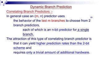
 The simplest and most common way to increase the ILP is
to exploit parallelism among iterations of a loop.
 This type of parallelism is often called loop-level
parallelism.
 Consider a simple example of a loop that adds two 1000-
element arrays and is completely parallel:
 for (i=0; i<=999; i=i+1)
x[i] = x[i] + y[i];
 Every iteration of the loop can overlap with any other
iteration
 Within each loop iteration there is little or no
opportunity for overlap.

 There are number of techniques for converting such loop-
level parallelism into instruction-level parallelism.
 Basically, such techniques work by unrolling the loop
 either statically by the compiler or
 dynamically by the hardware

Data Dependence
 Determining how one instruction depends on another is
critical to determine
 How much parallelism exists in a program
 How that parallelism can be exploited.
 To exploit ILP we must determine which instructions can
be executed in parallel.
 If two instructions are parallel, they can execute
simultaneously.
 If two instructions are dependent, they are not parallel and
must be executed in order, although they may often be
partially overlapped

Bernstein’s Conditins for detection of Parallelism
 Bernstein conditions are based on the following two sets of
variables:
i. The Read set or input set Ri that consists of variables
read by the statement of instruction Ii.
ii.The Write set or output set Wi that consists of variables
written into by instruction Ii .
 Two instructions I1 and I2 can be executed parallelly if
they satisfies the following conditions:
 R1 ∩ W2 = φ
 R2 ∩ W1 = φ
 W1 ∩ W2 = φ

Data Dependence
 Three different types of dependences:
 data dependences (also called true data dependences),
 name dependences and
 control dependences.
 Data Dependences
 True data dependence ( or flow dependence)
 Anti dependence
 Output dependence
 An instruction j is data dependent on instruction i if either of
the following holds:
 Instruction i produces a result that may be used by
instruction j, or
 Instruction j is data dependent on instruction k and
instruction k is data dependent on instruction i

Data Dependence
 Dependences are a property of programs
 Pipeline organization determines
 if dependence is detected and
 if it causes a stall
 Data dependence conveys 3 things:
 Possibility of a hazard
 Order in which results must be calculated
 An upper bound on howmuch parallelism can possibly
be exploited.
 A dependence can be overcome in two different ways:
 Maintaining the dependence but avoiding a hazard
 Eliminating the dependence by transforming the code.

Name Dependence
 Two instructions use the same name but no flow of
information associated with that name.
 Two types of Name Dependences between an instruction i
that precedes instruction j in program order
 1) Antidependence: instruction j writes a register or
memory location that instruction i reads.
 The original ordering must be preserved to ensure that
instruction i reads the correct value.
 2) Output dependence: instruction i and instruction j write
the same register or memory location
 Ordering must be preserved to ensure that the value
finally written corresponds to instruction j.
 To resolve name dependences, we use renaming techniques
(register renaming)

Module 2 of apj Abdul kablam university hpc.pdf

Data Hazards
 A hazard is created whenever there is a dependence
between instructions, and
 they are close enough that the overlap during execution
would change the order of access to the operand involved
in the dependence.
 Because of the dependence, we have to preserve the
program order.
 Three types of Data Hazards
 Read after write (RAW)
 Write after write (WAW)
 Write after read (WAR)

Data Hazards
 Read after write (RAW)
 Instruction j tries to read a source before i writes it, so j
incorrectly gets the old value.
 This hazard is the most common type
 It corresponds to a true data dependentce.
 Pgm order must be preserved to ensure that j receives
the value from i .
 Write After Write (WAW)
 Instruction j tries to write an operand before it is written
by i.
 The writes end up being performed in the wrong order.
 This corresponds to an output dependence

Data Hazards
 Write After Read (WAR)
 Instruction j tries to write a destination before it is read
by i, so i incorrectly gets the new value.
 This hazard arises from an antidependence.
 Read After Read (RAR) case is not a hazard.

Control Dependences
 A control dependence determines the ordering of an
instruction, i, w.r.t. a branch instruction so that the instruction
i executed in correct program order and only when it should
be.
 These control dependences must be preserved to preserve
program order.
 One of the simplest examples of a control dependence is the
dependence of the statements in the “then” part of an if
statement on the branch.

Control Dependences
 For example, in the code segment :
if p1 {
s1
}
if p2 {
s2
}
 S1 is control dependent on p1, and S2 is control dependent
on p2 but not on p1.

Control Dependences
 In general, two constraints are imposed by control
dependences:
 An instruction that is control dependent on a branch
cannot be moved before the branch so that its execution
is no longer controlled by the branch.
 For example, we cannot take an instruction from
the then portion of an if statement and move it
before the if statement.
 An instruction that is not control dependent on a branch
cannot be moved after the branch so that its execution
is controlled by the branch.
 For example, we cannot take a statement before
the if statement and move it into the then portion.

Basic Compiler Techniques for Exposing ILP
➢
These techniques are crucial for processors that use static
scheduling.
➢
The basic compiler techniques includes:
➢
Scheduling the code
➢
Loop unrolling
➢
Reducing branch costs with advanced brach
prediction

Basic Pipeline Scheduling
➢
To keep a pipeline full,
➢
parallelism among instructions must be exploited by
➢
finding sequences of unrelated instructions that
can be overlapped in the pipeline.
➢
To avoid a pipeline stall,
➢
the execution of a dependent instruction must be
➢
separated from the source instruction by a
distance in clock cycles equal to
➢
The pipeline latency of that source
instruction.

➢
A compiler’s ability to perform this scheduling depends
both on
➢
the amount of ILP available in the program and
➢
On the latencies of the functional units in the
pipeline.
Instruction
producing result
Instruction using
result
Latency in
clock cycles
FP ALU op Another FP ALU op 3
FP ALU op Store double 2
Load double FP ALU op 1
Load double Store double 0
➢
Latencies of FP operations used is given above.
➢
The last column is the number of intervening clock cycles
needed to avoid a stall.

➢
We assume
➢
the standard five-stage integer pipeline, so that
branches have a delay of one clock cycle.
➢
the functional units are fully pipelined or replicated (as
many times as the pipeline depth),
➢
so that an operation of any type can be issued on
every clock cycle and
➢
there are no structural hazards.
➢
The integer ALU operation latency of 0

➢
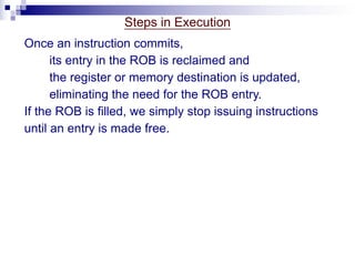
Consider the following code segment which adds a scalar
to a vector:
for (i=999; i>=0; i--)
x[i] = x[i] + s ;
➢
This loop is parallel by noticing that the body of each
iteration is independent.
➢
The first step is to translate the above segment to MIPS
assembly language.
➢
In the following code segment,
➢
R1 is initially the address of the element in the array
with the highest address, and
➢
F2 contains the scalar value s.
➢
Register R2 is precomputed, so that 8(R2) is the
address of the last element to operate on.

➢
The straightforward MIPS code, not scheduled for the
pipeline, looks like :
➢
Loop: L.D F0,0(R1) ;F0=array element
ADD.D F4,F0,F2 ;add scalar in F2
S.D F4,0(R1) ;store result
DADDUI R1,R1,#-8 ;decrement pointer
;8 bytes (per DW)
BNE R1,R2,Loop ;branch R1!=R2

➢
Without any scheduling, the loop will execute as follows:
Clock cycle issued
Loop: L.D F0,0(R1) 1
stall 2
ADD.D F4,F0,F2 3
stall 4
stall 5
S.D F4,0(R1) 6
DADDUI R1,R1,#-8 7
stall 8
BNE R1,R2,Loop 9

➢
We can schedule the loop to obtain only two stalls and
reduce the time to seven cycles:
Clock cycle issued
Loop: L.D F0,0(R1) 1
DADDUI R1,R1,#-8 2
ADD.D F4,F0,F2 3
stall 4
stall 5
S.D F4, 8(R1) 6
BNE R1,R2,Loop 7
➢
Two stalls after ADD.D are for use by the S.D

➢
In the previous example, we complete one loop iteration
and store back one array element every seven clock
cycles.
➢
The actual work of operating on the array element takes
just three (the load, add, and store) of those seven clock
cycles.
➢
The remaining four clock cycles consist of
➢
loop overhead—the DADDUI and BNE—and
➢
two stalls.
➢
To eliminate these four clock cycles
➢
we need to get more operations relative to the
number of overhead instructions.

Loop Unrolling
➢
A simple scheme for increasing the number of instructions
relative to the branch and overhead instructions is loop
unrolling.
➢
Unrolling simply replicates the loop body multiple times,
adjusting the loop termination code.
➢
Loop unrolling can also be used to improve scheduling.
➢
Because it eliminates the branch,
➢
it allows instructions from different iterations to be
scheduled together

Loop Unrolling
➢
If we simply replicated the instructions when we unrolled
the loop,
➢
the resulting use of the same registers could prevent
us from effectively scheduling the loop.
➢
Thus, we will want to use different registers for each
iteration,
➢
increasing the required number of registers.

Loop Unrolling without scheduling
➢
Here we assumes that the number of element is a multiple of 4.
➢
Note that R2 must now be set so that 32(R2) is the starting
address of the last four elements

Loop Unrolling without scheduling
➢
We have eliminated 3 branches and 3 decrements of R1 .
➢
Without scheduling, every operation in the unrolled loop is
followed by a dependent operation and thus will cause a
stall.
➢
This loop will run in 27 clock cycles:
➢
each L.D has 1 stall, (1x4 =4)
➢
each ADDD has 2 stalls, (2x4 =8)
➢
the DADDUI has 1 stall, (1x1 =1)
➢
plus 14 instruction issue cycles
➢
Or (27/4)=6.75 clock cycles for each elements.
➢
This can be scheduled to improve performance significally.

Loop Unrolling with scheduling

Loop Unrolling with scheduling
➢
The execution time of the unrolled loop has dropped to a
total of 14 clock cycles.
➢
or 3.5 clock cycles per element,
➢
compared with
➢
9 cycles per element before any unrolling or
scheduling
➢
7 cycles when scheduled but not unrolled.
➢
6.75 cycles with unrolling but no scheduling

Strip mining
➢
In real programs we do not usually know the upper bound on
the loop.
➢
Suppose it is n
➢
we would like to unroll the loop to make k copies of the body.
➢
Instead of a single unrolled loop, we generate a pair of
consecutive loops.
➢
The first executes (n mod k) times and has a body that
is the original loop.
➢
The second is the unrolled body surrounded by an outer
loop that iterates (n/k) times
➢
For large values of n, most of the execution time will be
spent in the unrolled loop body.

Loop Unrolling
➢
Loop unrolling is a simple but useful method for
➢
increasing the size of straight-line code fragments that
can be scheduled effectively.
➢
Three different effects limit the gains from loop unrolling:
(1) a decrease in the amount of overhead amortized with
each unroll
➢
If the loop is unrolled double the times(2n), the
overhead is reduced to 1/2 the overhead of
unrolling of n times.
(2) code size limitations
➢
growth in code size may increases instuction cache
miss rate
(3) compiler limitations – shortfall in registers.
- Register pressure

Branch Prediction
Loop unrolling is one way to reduce the number of branch
hazards.
We can also reduce the performance losses of branches
by predicting how they will behave.
Branch prediction schemes are of two types:
static branch prediction (or compile-time branch
prediction)
dynamic branch prediction

Static Branch Prediction
It is the simplest one, because
it does not rely on information about the dynamic
history of code executing.
It rely on information available at compile time
It predicts the outcome of a branch based solely on the
branch instruction.
i.e., uses information that was gathered before the
execution of the program.
use profile information collected from earlier runs.

Dynamic Branch Prediction
Predict branches dynamically based on program behavior.
It uses information about taken or not taken branches
gathered at run-time to predict the outcome of a branch.
The simplest dynamic branch-prediction scheme is a branch-
prediction buffer or branch history table.
A branch-prediction buffer is a small memory indexed by the
lower portion of the address of the branch instruction.
The memory location contains a bit that says whether
the branch was recently taken or not.

Different branch instructions may have the same low-order
bits.
With such a buffer we don’t know the prediction is correct
The prediction is a hint that is assumed to be correct, and
fetching begins in the predicted direction.
If the hint turns out to be wrong, the prediction bit is
inverted and stored back.
This simple 1-bit prediction scheme has a performance
shortcoming:
Even if a branch is almost always taken, we will likely
predict incorrectly twice, rather than once, when it is not
taken
since the misprediction causes the prediction bit to
be flipped.

2-bit Prediction Scheme :-
To overcome the weakness of 1-bit prediction scheme,
2-bit prediction schemes are often used.
In a 2-bit scheme, a prediction must miss twice before it is
changed.
Fig shows the finite-state diagram for a 2-bit prediction
scheme.

Correlating Branch Predictors :-
The 2-bit predictor schemes use only the recent behavior of
a single branch
to predict the future behavior of that branch.
It may be possible to improve the prediction accuracy
if we also look at the recent behavior of other
branches rather than just the branch we are trying to
predict.
Branch predictors that use the behavior of other branches to
make a prediction are called correlating predictors or two-
level predictors.

Consider the following code :
if (aa == 2) // branch b1
aa=0;
if (bb==2) // branch b2
bb=0;
if (aa!=bb) { // branch b3
........
}
The behavior of branch b3 is correlated with the behavior of
branches b1 and b2.
If branches b1 and b2 are both not taken then branch b3 will
be taken.

A predictor that uses only the behavior of a single branch to
predict the outcome of that branch can never capture this
behavior.
Existing correlating predictors add information about the
behavior of the most recent branches to decide how to
predict a given branch.
For example, a (1,2) predictor uses
the behavior of the last branch to choose from among a
pair of 2-bit branch predictors in predicting a particular
branch.

In general case an (m, n) predictor uses
the behavior of the last m branches to choose from 2
m
branch predictors,
each of which is an n-bit predictor for a single
branch.
The attraction of this type of correlating branch predictor is
that it can yield higher prediction rates than the 2-bit
scheme and
requires only a trivial amount of additional hardware.

The global history of the most recent m branches can be
recorded in an m-bit shift register,
where each bit records whether the branch was
taken or not taken.
The branch prediction buffer can then be indexed using
a concatenation of the low-order bits from the
branch address with the m-bit global history.

For example, in a (2, 2) buffer with 64 total entries,
the 4 low-order address bits of the branch (word address)
and
the 2 global bits representing the behavior of the two
most recently executed branches
form a 6-bit index that can be used to index the 64
counters.
The number of bits in an (m, n) predictor is
2
m
× n × Number of prediction entries selected by the
branch address
A 2-bit predictor with no global history is simply a (0,2)
predictor.

Tournament Predictors :-
Tournament predictors uses
multiple predictors,
usually one based on global information and
one based on local information, and
combining them with a selector.
Tournament predictors can achieve both
better accuracy at medium sizes (8K–32K bits) and
also make use of very large numbers of prediction bits
effectively.

Existing tournament predictors use a 2-bit saturating counter
per branch
to choose among two different predictors based on
which predictor (local, global, or even some mix) was
most effective in recent predictions.
As in a simple 2-bit predictor,
the saturating counter requires two mispredictions
before changing the identity of the preferred predictor.

The advantage of a tournament predictor is
its ability to select the right predictor for a particular
branch.

Fig: The misprediction rate for three different predictors on
SPEC89(benchmark) as the total number of bits is increased.

Speculation overcome control dependency
by
Predicting branch outcome and
Speculatively executing instructions as if
predictions were correct.
Hardware Based Speculation

Hardware-based speculation combines three key ideas:
1) dynamic branch prediction to choose which instructions
to execute
2) speculation to allow the execution of instructions before
the control dependences are resolved (with the ability
to undo the effects of an incorrectly speculated
sequence)
3) dynamic scheduling to deal with the scheduling of
different combinations of basic blocks.

Hardware-based speculation follows the predicted flow of
data values to choose when to execute instructions.
This method of executing programs is essentially a data
flow execution: Operations execute as soon as their
operands are available.

The key idea behind implementing speculation is to
allow instructions to execute out of order
but to force them to commit in order and
to prevent any irrevocable action (such as updating
state or taking an exception) until an instruction
commits.
Hence, when we add speculation,
we need to separate the process of completing
execution from instruction commit,
since instructions may finish execution
considerably before they are ready to commit.

Adding the commit phase to the instruction execution
sequence
requires an additional set of hardware buffers that
hold the results of instructions that have finished
execution but have not committed.
This hardware buffer, reorder buffer, is also used to pass
results among instructions that may be speculated.

• The reorder buffer (ROB) provides additional
registers.
• The ROB holds the result of an instruction
between the time the operation associated with
the instruction completes and the time the
instruction commits.
• Hence, the ROB is a source of operands for
instructions.
Reorder Buffer (ROB)

• With speculation, the register file is not
updated until the instruction commits ;
• thus, the ROB supplies operands in the
interval between completion of
instruction execution and instruction
commit.

Each entry in the ROB contains four fields:
the instruction type,
the destination field,
the value field, and
the ready field.
The instruction type field indicates whether the instruction
is
a branch (and has no destination result),
a store (which has a memory address destination), or
a register operation (ALU operation or load, which
has register destinations).

The destination field supplies
the register number (for loads and ALU operations) or
the memory address (for stores) where the instruction
result should be written.
The value field is used
to hold the value of the instruction result until the
instruction commits.
The ready field
Indicates that the instruction has completed execution,
and the value is ready.

Basic Structure with H/W Based Speculation

There are the four steps involved in instruction execution:
Issue
Execute
Write result
Commit
Steps in Execution

Issue
Get an instruction from the instruction queue.
Issue the instruction if there is an empty reservation
station and an empty slot in the ROB;
send the operands to the reservation station if
they are available in either the registers or the
ROB.
Update the control entries to indicate the buffers are
in use.
The number of the ROB entry allocated for the result
is also sent to the reservation station, so that the
number can be used to tag the result when it is
placed on the CDB (Common Data Bus).
Steps in Execution

Issue
If either all reservations are full or the ROB is full,
then instruction issue is stalled until both have
available entries.
Write Result :
When the result is available,
write it on the CDB (with the ROB tag sent
when the instruction issued) and from the CDB
into the ROB, as well as to any reservation
stations waiting for this result.
Mark the reservation station as available.
Steps in Execution

Write Result :
Special actions are required for store instructions.
If the value to be stored is available,
it is written into the Value field of the ROB entry
for the store.
If the value to be stored is not available yet,
the CDB must be monitored until that value is
broadcast, at which time the Value field of the
ROB entry of the store is updated.
Steps in Execution

Commit :
This is the final stage of completing an instruction,
after which only its result remains.
There are three different sequences of actions at
commit depending on whether the committing
instruction is
a branch with an incorrect prediction,
a store, or
any other instruction (normal commit)
Steps in Execution

Commit :
The normal commit case occurs when an instruction
reaches the head of the ROB and its result is present
in the buffer;
at this point, the processor updates the register
with the result and
removes the instruction from the ROB.
Committing a store is similar except that
memory is updated rather than a result register.
Steps in Execution

Commit :
When a branch with incorrect prediction reaches the
head of the ROB, it indicates that the speculation was
wrong.
The ROB is flushed and execution is restarted at the
correct successor of the branch.
If the branch was correctly predicted, the branch is
finished.
Steps in Execution

Once an instruction commits,
its entry in the ROB is reclaimed and
the register or memory destination is updated,
eliminating the need for the ROB entry.
If the ROB is filled, we simply stop issuing instructions
until an entry is made free.
Steps in Execution

Multithreading: Exploiting Thread-Level
Parallelism to Improve Uniprocessor Throughput
allows multiple threads to share the
functional units of a single processor in an overlapping
fashion.
In contrast, a more general method to exploit thread-
level parallelism (TLP) is with a multiprocessor that has
multiple independent threads operating at once and in
parallel.
Multithreading, however, does not duplicate the entire
processor as a multiprocessor does.
Instead, multithreading shares most of the processor
core among a set of threads, duplicating only
.

contd..
• Duplicating the per-thread state of a processor core
means creating a separate register file, a separate PC,
and a separate page table for each thread.
• There are three main hardware approaches to
multithreading.
1. Fine-grained multithreading switches between threads
on each clock, causing the execution of instructions
from multiple threads to be interleaved.
2. Coarse-grained multithreading switches threads only
on costly stalls, such as level two or three cache
misses.
3. Simultaneous multithreading is a variation on fine
grained multithreading that arises naturally when fine-
grained multithreading is implemented on top of a
multiple-issue, dynamically scheduled processor.

. The horizontal dimension represents the
instruction execution capability in each clock cycle. The vertical
dimension represents a sequence of clock cycles. An empty (white) box
indicates that the corresponding execution slot is unused in that clock
cycle. The shades of gray and black correspond to four different threads
in the multithreading processors.

Module 2 of apj Abdul kablam university hpc.pdf

More Related Content

Similar to Module 2 of apj Abdul kablam university hpc.pdf (20)

Recently uploaded (20)

Module 2 of apj Abdul kablam university hpc.pdf