Applied numerical methods lec10

2
Methods for Numerical Integration

3
Newton-Cotes Formulas
Approximate integrand function f(x) by a polynomial that can then be easily integrated

5
The Trapezoidal Rule
( ) ( )dxxfdxxf
b
a
b
a ∫∫ ≅= 1I
( ) ( ) ( ) ( )( )a-x
a-b
afbf
afxf
−
+=1
( ) ( ) ( )( ) ( ) ( ) ( )
2
bfaf
abdxa-x
a-b
afbf
afI
b
a
+
−=




 −
+= ∫
All the Newton-Cotes formulas can be expressed in this general average height form
heightaveragewidthI ×≅

Example 1 Single Application of the Trapezoidal Rule
f(x) = 0.2 +25x – 200x2 + 675x3 – 900x4 + 400x5
Integrate f(x) from a=0 to b=0.8
%....E
.
..
.
)()(
)(
tt
:oferroranrepresentswhich
:RulelTrapezoida
58946773117280640531
17280
2
232020
80
2
==−=
=
+
=
+
−=
ε
bfaf
abI
∫
=
=
==
80
0
640531
.
.)(:valueintegralTrue
b
a
dxxfI
Solution: f(a)=f(0) = 0.2 and f(b)=f(0.8) = 0.232

7
• The accuracy can be improved by dividing the
interval from a to b into a number of segments
and applying the method to each segment.
• The areas of individual segments are added to
yield the integral for the entire interval.
Using the trapezoidal rule, we get:
∫∫∫
−
+++=
===
−
=
n
n
x
x
x
x
x
x
n
dxxfdxxfdxxfI
xbxa
n
ab
h
1
2
1
1
0
)()()(
seg.of#n 0
L






++
−
=
+
++
+
+
+
=
∑
−
=
−
1
1
0
12110
2
2
222
n
i
in
nn
xfxfxf
n
ab
I
xfxf
h
xfxf
h
xfxf
hI
)()()(
)()()()()()(
L
The Multiple-Application Trapezoidal Rule

Example 4
The vertical distance covered by a rocket from to seconds is
given by:
∫ 





−



−
=
30
8
89
2100140000
140000
2000 dtt.
t
lnx
a) Use two-segment Trapezoidal rule to find the distance covered.
b) Find the true error, for part (a).
c) Find the absolute relative true error, for part (a).a∈
tE

Solution
a) The solution using 2-segment Trapezoidal rule is






+






++
−
= ∑
−
=
)b(f)iha(f)a(f
n
ab
I
n
i
1
1
2
2
2=n 8=a 30=b
2
830 −
=
n
ab
h
−
= 11=

Solution (cont)






+






++
−
= ∑
−
=
)(f)iha(f)(f
)(
I
i
3028
22
830 12
1
[ ])(f)(f)(f 301928
4
22
++=
[ ]6790175484227177
4
22
.).(. ++=
m11266=
Then:

Solution (cont)
∫ 





−



−
=
30
8
89
2100140000
140000
2000 dtt.
t
lnx m11061=
b) The exact value of the above integral is
so the true error is
ValueeApproximatValueTrueEt −=
1126611061−=

Solution (cont)
The absolute relative true error, , would bet∈
100
ValueTrue
ErrorTrue
×=∈t
100
11061
1126611061
×
−
=
%8534.1=

Solution (cont)
Table 1 gives the values
obtained using multiple
segment Trapezoidal rule for
n Value Et
1 11868 -807 7.296 ---
2 11266 -205 1.853 5.343
3 11153 -91.4 0.8265 1.019
4 11113 -51.5 0.4655 0.3594
5 11094 -33.0 0.2981 0.1669
6 11084 -22.9 0.2070 0.09082
7 11078 -16.8 0.1521 0.05482
8 11074 -12.9 0.1165 0.03560
∫ 





−



−
=
30
8
89
2100140000
140000
2000 dtt.
t
lnx
Table 1: Multiple Segment Trapezoidal Rule Values
%t∈ %a∈
Exact Value=11061 m

Applied numerical methods lec10

)()(
)(
)(
2
2
1
212
2
2
1
2
1






≅⇒≅
h
h
hEhE
h
h
hE
hE
Romberg Integration
Successive application of the trapezoidal rule to attain efficient numerical integrals of functions.
Richardson’s Extrapolation:
Uses two estimates of an integral to compute a third and more accurate approximation.
sizes)stepdifferentforconstantis(assume
)()()()(
/)(/)()()(
)
2
(
2
12
2211
fhOfh
ab
E
hEhIhEhI
habnnabhhEhII
′′=′′
−
≅
+=+
−=−=+=
I = exact value of integral E(h) = the truncation error
I(h): trapezoidal rule (n segments, step size h)
Improved estimate of the integral.
It is shown that the error of this
estimate is O(h4). Trapezoidal rule
had an error estimate of O(h2).( )
[ ])()(
/
)(
)()(
122
21
2
22
1
1
hIhI
hh
hII
hEhII
−
−
+≅
+=
( )
( ) 1/
)()(
)()()(/)()( 2
21
12
222
2
2121
−
−
≅⇒+≅+
hh
hIhI
hEhEhIhhhEhI

25
( )
[ ])()(
1/
1
)( 122
21
2 hIhI
hh
hII −
−
+≅
Example 7
Evaluate the integral of f(x) = 0.2 +25x – 200x2 + 675x3 – 900x4 + 400x5
from a=0 to b=0.8. I (True Integral value) = 1.6405
Segments h Integral εtr%
1 0.8 0.1728 89.5
2 0.4 1.0688 34.9
4 0.2 1.4848 9.5
%)6.16(0.2733675.16405.1E
3675.1)1728.0(
3
1
)0688.1(
3
4
:givetocombined2&1Segments
tt ==−=
=−≅
ε
I
In each case, two estimates with
error O(h2) are combined to give a
third estimate with error O(h4)
%)1(0.01716234.16405.1E
6234.1)0688.1(
3
1
)4848.1(
3
4
:givetocombined4&2Segments
tt ==−=
=−≅
ε
I
)2/(If 12 ⇒= hh [ ] )(
3
1
)(
3
4
)()(
12
1
)( 121222 hIhIhIhIhII −=−
−
+≅

26
Simpson’s Rules
General idea:
Use high order polynomials other than trapezoids to achieve more
accurate integration result but using the similar amount of computation
Parabola Cubic polynomial

• More accurate estimate of an integral is obtained if
a high-order polynomial is used to connect the
points. These formulas are called Simpson’s rules.
Simpson’s 1/3 Rule: results when a 2nd order
Lagrange interpolating polynomial is used for f(x)
dxxf
xxxx
xxxx
xf
xxxx
xxxx
xf
xxxx
xxxx
I
dxxfdxxfI
x
x
b
a
b
a
xbxa
xf
∫
∫ ∫






−−
−−
+
−−
−−
+
−−
−−
=
≅=
==
2
0
)(
))((
))((
)(
))((
))((
)(
))((
))((
)()(
2
1202
10
1
2101
20
0
2010
21
20
2
Using
.polynomialorder-secondais)(2where
[ ] RULE1/3SSIMPSON'
2
)()(4)(
3
210
:resultsformulafollowingtheon,manipulatialgebraicandnintegratioafter
⇐
−
=++≅
ab
hxfxfxf
h
I
a=x0 x1 b=x2
Simpson’s Rules

28
[ ] RULE1/3SSIMPSON'
2
)()(4)(
3
210
:resultsformulafollowingtheon,manipulatialgebraicandnintegratioafter
⇐
−
=++≅
ab
hxfxfxf
h
I

30
Trapezoidal vs. Simpson’s 1/3 Rule
( ) ( ) ( ) ( ) 3674671
2
8080 .
.
..I =
++
=
++
≅
6
0.2322.45640
6
0.8f0.44f0f
%.616=→== tt 0.27306671.367467-1.640533E ε
Trapezoidal:
Example: f(x) = 0.2 + 25x – 200x2 + 675x3 – 900x4 + 400x5 (integral between a=0 and b=0.8)
( ) ( ) ( ) 0.1728
2
0.8f0f
00.8 =
+
−≅I
Et = 1.640533 – 0.1728 = 1.467733 εt = 89.5%
Simpson’s 1/3 rule:

32
Multiple Application of Simpson’s 1/3 Rule

38
[ ]
8
)()(3)(3)(
)(
)()(3)(3)(
8
3
)()(
3210
3210
3
3
)(
xfxfxfxf
abI
xfxfxfxf
h
I
dxxfdxxfI
ab
h
b
a
b
a
+++
−≅
+++≅
≅=
−
=
∫ ∫
Simpson’s 3/8 Rule
Simpson’s 1/3 and 3/8 rules can be
applied in tandem to handle
multiple applications with odd
number of intervals
Fit a 3rd order Lagrange interpolating
polynomial to four points and integrate

Gauss Quadrature
• Gauss quadrature implements a strategy of
positioning any two points on a curve to define a
straight line that would balance the positive and
negative errors.
• Hence the area evaluated under this straight line
provides an improved estimate of the integral.

Method of Undetermined Coefficients
• The trapezoidal rule yields exact results when the function
being integrated is a constant or a straight line, such as y=1
and y=x:
)()( 10 bfcafcI +≅
)(
2
)(
2
2
0
22
22
110
10
10
10
2/)(
2/)(
10
2/)(
2/)(
bf
ab
af
ab
I
ab
cc
ab
c
ab
c
abcc
dxx
ab
c
ab
c
dxcc
ab
ab
ab
ab
−
+
−
=
−
==
=
−
+
−
−
−=+
=
−
+
−
−
=+
∫
∫
−
−−
−
−−
Solve simultaneously
Trapezoidal rule

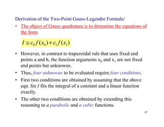
47
Derivation of the Two-Point Gauss-Legendre Formula/
• The object of Gauss quadrature is to determine the equations of
the form
• However, in contrast to trapezoidal rule that uses fixed end
points a and b, the function arguments x0 and x1 are not fixed
end points but unknowns.
• Thus, four unknowns to be evaluated require four conditions.
• First two conditions are obtained by assuming that the above
eqn. for I fits the integral of a constant and a linear function
exactly.
• The other two conditions are obtained by extending this
reasoning to a parabolic and a cubic functions.
)()( 1100 xfcxfcI +≅

Solved simultaneously






+




 −
≅
−==
−=−=
==
3
1
3
1
5773503.0
3
1
5773503.0
3
1
1
1
0
10
ffI
x
x
cc
K
K
Yields an integral
estimate that is third
order accurate

49
Two-Point Gauss-Legendre Formula
(arbitrary a and b)
( ) ( )
bxx
ax-x
2
xabab
x
d
dd
=→=
=→=


−++
=
1
1
( )∫=
b
a
dxxfI
( ) ( ) ( ) ( )
∫
=
=





 −++





 −++
=
1x
-1x
ddd
d 2
xabab
d
2
xabab
fI
( ) ( )
∫ 




 −++−
=
1
1- d
d
dx
2
xabab
f
2
ab
I

50
Example of Two-Point Gauss-Legendre Formula
( ) 8225781264592532918525140
3
1
3
1
40 ....ff.I dd =+=
















+






 −
=
( ) ( )∫∫ +==
1
1-
0.8
0 dd dx0.4x0.4f0.4dxxfI
( )∫=
1
1- ddd dxxf40.I
Example14: f(x) = 0.2 + 25x – 200x2 + 675x3 – 900x4 + 400x5 (integral between a=0 and b=0.8)
x = 0.4 + 0.4xd
dx = 0.4 dxd
( ) ( ) ( ) ( ) ( )[ ]∫ +++−+++−++=
1
1- dddddd dx0.4x0.40.4x0.40.4x0.40.4x0.40.4x0.4250.20.4
543
400900675200 2
I
( ) ( )
bxx
ax-x
2
xabab
x
d
dd
=→=
=→=


−++
=
1
1
)()( 1100 xfcxfcI +≅

51
Higher-Point Gauss-Legendre Formula
( ) ( ) ( )[ ]2d21d10d0 xfcxfcxfc ++= 40.I
( ) ( ) ( ) ( )
44444444 344444444 21
L
44444 344444 21
444 3444 21
pointn
1-n1-n
pointthree
22
pointtwo
1100 xfcxfcxfcxfc
−
−
−
++++≅I
( )∫=
1
1- ddd dxxf40.I
Example: f(x) = 0.2 + 25x – 200x2 + 675x3 – 900x4 + 400x5 (integral between a=0 and b=0.8)
Three-point Gauss-Legendre formula: c0 = 0.5555556 x0 = - 0.774596669
c1 = 0.8888889 x1 = 0.0
c2 = 0.5555556 x2 = 0.774596669
( ) ( ) ( )[ ].77459669f0.5555560f0.88888890.77459669-f0.5555560.4 ddd ++=I
1.640533

54
( ) 543376.0318386.0768365.05.0
3
1
3
1
5.0 =+=











+




 −
= dd ffI
( ) ( ) ( )( )
( ) 0.5405910.275778*0.55555560.494845*0.88888890.878598*0.55555565.0
90.77459666*0.55555560.0*0.888888990.77459666-*0.55555565.0
=++=
++= ddd fffI

55
Gauss Quadrature
Gauss-Chebyshev Formula

56
Gauss Quadrature
Gauss-Hermite Formula

57
Integration Using Matlab
Approximation of Double Integrals Using Matlab

Applied numerical methods lec10

More Related Content

What's hot (20)

Similar to Applied numerical methods lec10 (20)

More from Yasser Ahmed (14)

Recently uploaded (20)

Applied numerical methods lec10