Dynamic Pricing for Personal Unsecured Loans

Price Sensitivity (0.1)
Towards 1:1 pricing

Modern/dynamic pricing approaches applied to personal unsecured loans (PUL).
Paul Golding, Dec 2018 @pgolding

Preface
• We want to predict a borrower’s sensitivity to price and use this information to
optimize prices to achieve maximum expected profit (or some other business
goal - TBD)

• This deck is a “think aloud” conversation to gain a common understanding of the
principles and possible solutions to the pricing sensitivity problem. It also poses
questions that need answers to move forward with building a pricing model.

• The deck contains a mostly mathematical tour of the principles because the goal
is to discover a computational method(s) that might achieve 1:1 pricing
segmentation via a fully automated system.

• We heavily lean upon the work of R. Phillips’ (Pricing Credit Products) and
referenced materials. A literature review suggests that his work is a definitive
baseline. In places, we have formulated the math in a more accessible fashion.

Credit Risk
1. Risk is a variable cost

2. Risk is correlated with price sensitivity: riskier customers tend to be less
price sensitive

3. Price influences risk: all else equal, raising prices leads to higher losses -
price-dependent risk.

Terms
• Exposure at Default (EAD) - remaining balance at default

• Loss Given Default (LGD) = EAD/Total Loan Amount

• Probability of Default (PD) = P(Default) | t<=loan_term

• EAD and LGD are random variables

• (Note: we largely stick to Phillips’ terminology to be consistent with his
theoretical foundations. Variation from more standard terminology is
noted.)

Expected Loss
We care about expected values of random vars
PD = pd
(t)
t=1
T
∑
EEAD =
pd
(t) × EADt
t=1
T
∑
PD
ELGD =
pd
(t) × EADt
t=1
T
∑ × LGDt
pd
(t) × EADt
t=1
T
∑
EL = pd
(t) × EADt
t=1
T
∑ × LGDt
∴ EL = PD × ELGD × EEAD
Probability of default at t=1 or t=2 or t=3 … or t=T
Expected loss is major determinant of
expected profitability of a loan and
thereby influences price.

Simplified Pricing Threshold
E π
( )= 1− PD
( ) p − pc
( )− PD × (1+ pc ) One-period supply capital rate pc
One-period price p
Expected profit for $1 1-period loan (to simplify understanding risk/price relationship):
profit loss
p >
PD 1+ pc
( )
1− PD
+ pc
cost of capital
Risk-adjusted premium
This only suggests a lower bound.

It does not suggest the price:

• Maximize profitability?

• Maximize bookings subject to profit constraint?

• Price sensitivity of customer
Extremely simplified: ignores dynamics of payment/
default in multi-period loan and that PD is not
independent of price at which loan offered. But sufficient
to show the role of risk.
A function of PD
pc =0.1
Risk cut-off equation:

Risk Prediction
s x
( )= ln
Pr{G | x}
Pr{B | x}
⎛
⎝
⎜
⎞
⎠
⎟
score of observables vector log odds (i.e. monotonic)
modeled using ML
(e.g. XGBoost)
Presumably decision-tree based for reasons of interpretability (actual adverse actions methodology: see D. Paulsen).

(Look ahead: can we get better sensitivity predictions if we don’t care about interpretability?)
P̂{B | x}

Risk Factors
P̂{B | x} • Risk prediction based upon borrower
observables

• But also the loan itself

• Amount

• Leverage (e.g. LTV, DTI)

• Period (longer loans riskier due to information
asymmetry, random shock etc.)

• And price-dependent risk
Not part of x
Borrower dependent risk
Product dependent risk

Price-dependent Risk
If for all values of
E π
( )= 1− PD
( ) p − pc
( )− PD × (1+ pc )
⇒ E π
( )= 1− PD p
( )
( ) p − pc
( )− PD p
( )× (1+ pc )
P ′
D p
( )> 0 i.e. positive slope, or risk increases with price
PD p
( )>
p − pc
p +1
p ≥ pc
then there is no price at which a loan is profitable

Price-dependent Risk
• Fraud - fraudulent borrowers are insensitive to price

• Adverse private information - e.g. unobservable knowledge of a
borrower’s forthcoming redundancy

• Competitive alternatives - less riskier customers have more options and
so loans at a certain (higher) price will attract riskier borrowers

• Behavioral factors - behavioral economics, mental accounting, time
discounting etc. (Dynamic contextual factors unrelated to loan
characteristics or borrower credit-worthiness attributes.)

• Aﬀordability - e.g. DTI (capacity to pay)

Incremental Profitability
• Optimal price imposes two questions:

• How will profitability of a loan change with price?

• How will demand for a loan change with price?

• Profitability for loans non-trivial calculation due to:

• Time value of money (discounted value of future costs/revenues)

• Uncertainty: default, prepayment, utilization (for credit line)

• We need a model for incremental profitability for PUL

• What are the variable costs? (Holds, channels?)

• What is the profit goal? (For whom?)

• If we sell/securitize loans, how does this aﬀect optimization?

• Longer loans are more profitable (via interest)

• Large-portfolio holders should act more risk-neutral (assuming risk of loans are statistically independent across
the portfolio) - see Phillips

• Also: should pricing model take LTV into account - e.g. cross-selling other products?  
(Segmentation question?)
Action: construct the incremental profitability model

Price Response Curve
• We want to know the price-
response function per product
per segment (vs. market-
demand curve per product) - i.e.
their Willingness To Pay (WTP)

• Price optimization uses this along
with expected incremental profit
calculation to price for maximum
expected total profitability (for a
loan portfolio)
d p
( )= DF p
( )
total applications

(i.e. “market size”)
take-up rate (i.e. WTP)
price-response

(i.e. “demand”)
Adapted from curve in this paper: Journal of Business Research
Loan APR
Loan APR
F p
( )= f w
( )dw
p
∞
∫
probability distribution of WTP

WTP is probability of a customer paying

at most p - i.e. note that it is the complementary

cum. dist. func. or 1 - F(p) (often seen in the literature)
D = d(0) - i.e. willing to buy at all

(source: DTU ME)
Additional source: BPO lecture notes.
Nominal demand curve
(closed form continuous)
In general, d(p) = D ( 1-F(p) ) = D(F(infinity)-F(p)).

Some derivations
d p
( )= DF p
( )⇒ ′
d p
( ) = −D ′
F p
( )= Df p
( )
F p
( )= f w
( )dw
p
∞
∫ ⇒ − ′
F p
( )= f p
( )
For a given WTP curve, the corresponding density
Slope -ve, hence introduce minus sign
In some cases, we are interested in absolute slope of the take-up rate, in which case:
′
F p
( )⇒ ′
d p
( ) / D = f p
( )
Note: the derivative can be interpreted as the percentage willing to pay exactly p:
′
F p
( )≈
F(p + h)− F(p)
F(p)
For small h

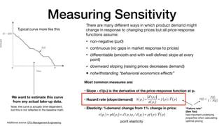
Measuring Sensitivity
Typical curve more like this
Note: the curve is actually time-dependent,

but this is not reflected in the baseline math.
There are many different ways in which product demand might
change in response to changing prices but all price-response
functions assume:

• non-negative (p≥0)

• continuous (no gaps in market response to prices)

• differentiable (smooth and with well-defined slope at every
point)

• downward sloping (raising prices decreases demand)

• notwithstanding “behavioral economics effects”
Additional source: DTU Management Engineering
Most common measures are:
• Slope - d’(p1) is the derivative of the price-response function at p1
• Hazard rate (slope/demand)
• Elasticity: %demand change from 1% change in price:
ε p1
( )= ph p1
( )= ′
d (p1)p1 / d p1
( )= pf p
( )/ F p
( )
h p1
( )=
′
d (p1)
d p1
( )
= f p
( )/ F p
( )
point elasticity
We want to estimate this curve
from any actual take-up data.
“Failure rate”
(See Yao)
has important underlying
properties when calculating
optimal pricing.

Sensitivity and risk
• As said, higher prices = higher default rates AND higher risk customers are less price sensitive (e.g. price
elasticity higher for higher FICO)

• But the two phenomenon are the same: if price sensitivity decreases with risk in a population, then the
populate will demonstrate price-dependent risk.
db p
( )= DbFb p
( )
D = Dg + Db
dg p
( )= DgFg p
( )
#applicants take-up rate
#goods #bads
DR = Db / Dg + Db
However, the rate is price dependent, so: DR(p) =
DbFb p
( )
DbFb p
( )+ DgFg p
( )
Diﬀerentiating wrt price, we get: D ′
R p
( )= (hg p
( )− hb p
( ))DR p
( )(1− DR p
( ))
failure rate diﬀerence between
goods and bads
hg p
( )= − ′
Fg p
( )/ Fg p
( )= fg p
( )/ Fg p
( )
hb p
( )= − ′
Fb p
( )/ Fb p
( )= fb p
( )/ Fb p
( )
via substitution, chain-rule

and product rule

Sensitivity and risk
D ′
R p
( )= z p
( )DR p
( )(1− DR p
( ))
z p
( )= hg p
( )− hb p
( ) Difference in hazard rate
Price-dependent risk rate (or PDR rate) - i.e. rate at which risk changes with price
commercial lending region
for constant
z(p) and
z(p)>0
In this part of the curve, price-dependent risk more salient for

higher-risk populations.

“As found in practice - i.e. effect of price on risk much stronger in sub-
prime than prime. Very little impact in super prime.”

What does it imply for pricing? Net interest income for a loan of value
1 (for simplicity) and loss-given default:
Π p
( )= (p − c)dg p
( )− ldb p
( )
0 < l ≤1
There is a positive number k such that z(p)>k for all p >=c in which case the lender cannot achieve a profit at any price.
Whether or not it is profitable to offer a loan depends not only on bads:goods but on their difference in price sensitivity as
reflected in the differential hazard rate z(p)

Pricing/Underwriting
Π p
( )= (p − c)dg p
( )− ldb p
( )
There is a positive number k such that z(p)>k for all p >=c in which
case the lender cannot achieve a profit at any price.
Whether or not it is profitable to offer a loan depends not only on
bads:goods but on their difference in price sensitivity as reflected in
the differential hazard rate z(p)
k = hb p
( )− hg p
( )

Estimating d(p)
• We assume a data-driven approach based upon random testing (of
prices), but we need to evaluate the current random-testing method/data

• Are we storing all endogenous variables? (if any)

• Do we have suﬃcient test data for each segment?

• (Note: we can model using available data and also estimate with
piecewise numerical estimator - see later.)

• Given the historical data, we now estimate a price-response model using
ML (GLMs or ANN?)

• Do we have endogeneity?

• What might cause it? e.g. agent intervention in the sale of the loan

Model
• Considerations

• Feature selection (for price sensitivity)

• Feature engineering overhead

• Monotonicity - The assumption of pricing optimization is that prices change monotonically

• Can we short-cut feature engineering stage with use of a novel DL method, like Deep Lattice
Networks?

• Pros: shortcut feature engineering, Tensorflow models, organizational learning

• Cons: lack of proven field experience (with DLN). Expertise better used elsewhere (portfolio
optimization?)
• Updating: frequency and method (to track temporal changes)

• To what extent can this be automated?

• Should we include other product co-joint analysis?  
(“Price to entice” as gateway to higher LTV.)

Pricing Segmentation
M Product dimensions
(e.g. amount, term)
N Customer dimensions
(e.g. scores, employment)

observable/explainable
Price - Price -
- Price Price -
- Price Price
- - - Price
NxM buckets
(upper bound)

logical limit 1:1 pricing

or.. NxM dimensional surface

whose geometry determines revenue/profit

and should be correlated to:

• incremental profitability

• price sensitivity
• Smaller (more targeted) buckets => profitability, but also
complexity. What is the trade-off? (We need to do work to
analyze the frontier of ROI trade-off curves.)

• All else being equal, charge lower prices to segments with:

• higher inc. profitability

• higher price sensitivity

• other business incentive e.g. promote certain
channels? (Again, what are the business constraints.)
• Customer dimensions:

• Risk, [age], loyalty, [geography] etc.

• Product dimensions:

• Loan amount, term

• Term - should we consider a higher resolution of term (than
just 3/5 year) to obtain better results? (And give a more
satisfactory UX.)?

Are there other ways to differentiate product besides price? e.g. “no-charge term rescheduling or repayment rewards”

i.e. customer segmentation achieved via product segmentation correlated to price sensitivity

WTP: Pricing
Demand
Price
Demand
Price
Demand
Price
p* p1* p2*
c c c
Single price p*

missed revenue = A,B
Two prices c<p1*<p2*

missed = A,B,C
1:1 pricing

missed = “0”
• We now see the importance of predicting WTP = revenue/profit

• However, WTP extends beyond risk-based customer variables e.g. to include things like financial
sophistication, brand aﬃnity, urgency, competitive environment etc.

• Note: are some of these observable, say via random experiments in design (or other means). Do we
capture all the necessary data? What other data sources can we use?

• i.e. pricing (sensitivity) is not a “backend” function only

• Can we gather more user data? (e.g. for DM clients can we aﬀord “second stage?”)

online tasks
Dynamic segmentation
Query $
Price
Dims
Optimization
Prices for all

segments
offline tasks
Optimization $
Offer Offer
Application Application
Analysts
reviewers
• d(p) can be continually computed (and “event driven”)

• New data resolution (higher freq)

• Market shifts (lower freq)

• What are the operational implications of moving to a 1:1
model?

• To what extent can the entire process be automated?

• Optimization model (inc. freq)

• Operational model (as an operationally acceptable rule-
based system - what are the constraints?)

• Can/do we capture all the data we need (e.g. UX state)?

• What is the limit at which other approaches should be
considered (due to behavioral economics factors)?

• The exact nature and implementation of the current offline
tasks need to be audited and automation ROI calculated
Compute power is cheap. If we can find an end-to-end computational solution, even highly complex (AI), it potentially pays!
What are the strategic (tech) imperatives in a commodity PUL market?

Optimizing Prices (Simple loan)
E π p
( )
( )= F p
( )[ 1− PD
( )× p − c
( )− PD × l]
Consider a single two-period loan (just makes math simpler initially) [And assume LGD independent of price, which it is not.]
l = LGD + c
[simplistic incremental profit]
price response
= F p
( )[ 1− PD
( )× p − c −
l
o
⎛
⎝
⎜
⎞
⎠
⎟] o = (1− PD) / PD odds that loan will not default
loss given default
cost of funds
⇒ o*
=
LGD + c
p − c
underwriting criterion for a price-taking lender - i.e. take any loans with odds > o*
But we are interested in price-setting lender. In which case we want to charge a price p* that would maximize

Here we omit the analytical solution for as there is no closed-form solution for any non-linear price response function.

Rather, we can see that if we can compute then we can calculate the maximum using numerical methods.
E π p
( )
( )
′
E π p
( )
( )
F p
( )

Price-dependent risk
Analytical solution for
h p*
( )=
1
p*
− c −
l
o
′
E π p
( )
( )= 0
But we have so far assumed that PD and loss are independent of price of loan, which is incorrect.

If we now assume that we have a population Dg of good and Db bad customers.
E π p
( )
( )= Fg p
( )Dg p − c
( )− Fb p
( )Dbl
′
E π p
( )
( ) ′
E =0
⎯ →
⎯⎯ hg p*
( )=
1
p*
− c −
fb p*
( )
fg p*
( )
⎛
⎝
⎜
⎞
⎠
⎟
l
o0
⎛
⎝
⎜
⎞
⎠
⎟
This holds for price-dependent risk (diﬀerent dist. for bads/goods)
′
E π p
( )
( ) ′
E =0
⎯ →
⎯⎯ hg p̂
( )=
1
p̂ − c −
l
o p̂
( )
⎛
⎝
⎜
⎞
⎠
⎟
If we assume the odds will not change (i.e. ignore price-dependent risk)
BUT: we do expect goods have higher failure rate => fb p
( )/ fg p
( )> Fb p
( )/ Fg p
( )
And therefore (plugging into above equations):

Which means the (amateur) lender who does not consider influence of price upon risk will set a price that is higher than the
expert lender, which means higher losses and lower profit. Note: this aﬀects competitors profitability - see Nomis white paper.
p*
< p̂
population odds

Adaptive Optimization
1. Iterate k pricing adjustments α1 > α2 > α3...> 0
2. Use 2-point price estimation (testing) to estimate ĥ pk
( )= 2 d1D2 − d2D1
( )/[δ d1D2 + d2D1
( )
( )]
3. Calculate price gap g(pk ) = ĥ pk
( )−1/(pk − c − l / o)
4. if − ε ≤ g(pk ) ≤ ε set p*
= pk and stop
5. if g(pk ) < −ε set pk+1 = pk +αk and go to step 2
6. if g(pk ) > ε set pk+1 = pk −αk and go to step 2
1/ p − c − l / o
( )
h p
( ) assumed unknown
c + l / o r*
ε
ε
p
Raise Hold Lower
inverse margin
What if we don’t know h(p)?

Optimization Over Segments
p*
= argp max DF p
( )π p
( )
( )
!
p*
= argp max DiFi pi
( )πi pi
( )
i=1
N
∑
⌣
"
p = argp max DiFi pi
( )Ri pi
( )
i=1
N
∑
!
p = argp max DiFi pi
( )πi pi
( )
i=1
N
∑ + DiFi pi
( )Ri pi
( )
i=1
N
∑
⎡
⎣
⎢
⎤
⎦
⎥
Or with constraints:
e.g Bounds, structural constraints, monotonicity of pricing, segment bounds, rate endings
!
p = argp max ΦC ( DiFi pi
( )θi pi
( )
i=1
N
∑ )
⎡
⎣
⎢
⎤
⎦
⎥
c=1
M
∑
⎡
⎣
⎢
⎤
⎦
⎥
Subject to feasibility whilst trying to avoid post-hoc pricing adjustments (“overlays”) due to “shortcomings” in the model.

And subject to idealized segmentation (that avoids mixed [separable] failure curves with implied lack of global maximum).

And subject to location of the portfolio on the eﬃcient frontier (next).

Where/what are the automation opportunities for constraint review and management?
(assume independently solvable)

Efficient Frontier
Return
Risk
• We can estimate the frontier and where our portfolio lies within it

• But we may have chosen unrealistic (or too many) constraints

• We might have chosen constraints outside of the model (i.e. tuned prices manually)

• Optimal portfolio selection is an area of R&D opportunity (reinforcement learning, genetic algorithms, etc.)

• Optimal segmentation is also an area for R&D opportunity
Can I have the highest revenue with greatest profit and lowest risk please? No.

Dynamic Pricing for Personal Unsecured Loans

More Related Content

What's hot (18)

Similar to Dynamic Pricing for Personal Unsecured Loans (20)

More from Paul Golding (20)

Recently uploaded (20)

Dynamic Pricing for Personal Unsecured Loans