SlideShare a Scribd company logo
Vertical Curves
Chapter 25
Profiles:
Curve a: Crest Vertical Curve (concave
downward)
Curve b: Sag Vertical Curve (concave
upward)
Tangents: Constant Grade (Slope)
Equal-Tangent Vertical
Parabolic Curve:
Terms:
BVC: Beginning of Vertical Curve aka PVC
V: Vertex aka PVI
EVC: End of Vertical Curve aka PVT
g1: percent grade of back tangent
g2: percent grade of forward tangent
L: curve length (horizontal distance) in feet or
stations
x: horizontal distance from any point on the curve
to the BVC
Equations:
r = (g2 – g1)/L
where:
g2 & g1 - in percent (%)
L – in stations
and
Y = YBVC + g1x + (r/2)x2
where:
YBVC – elevation of the BVC in feet
Example: Equal-Tangent
Vertical Curve
Given the information show below,
compute and tabulate the curve for
stakeout at full 100’ stations.
Solution:
L = STAEVC –
STABVC
L = 4970 –
4370 = 600’
or 6 full
stations
r = (g2 – g1) /
L
r = (-2.4 – 3) /
6
r = -0.90
r/2 = -0.45 % per station
STABVC = STAVertex – L / 2 = 4670 – 600/2 = STABVC =
STA 43 + 70
STAEVC = STAVertex + L / 2 = 4670 + 600/2 = STAEVC =
STA 49 + 70
Elev = Elev – g (L/2) = 853.48 – 3.00 (3) =
Solution:
(continued)
r/2 = -0.45 % per station
Elevx = ElevBVC + g1x + (r/2)x2
Elev44+00 = 844.48 + 3.00(0.30) –0.45(0.30)2
=
845.34’
Elev45+00 = 844.48 + 3.00(1.30) –0.45(1.30)2
=
847.62’
Elev46+00 = 844.48 + 3.00(2.30) –0.45(2.30)2
=
849.00’
etc.
Elev49+00 = 844.48 + 3.00(5.30) –0.45(5.30)2
=
847.74’
Solution:
(continued)
Station x
(station
s)
g1x r/2
x2
Curve
Elevatio
n
43 + 70
BVC
0.0 0.00 0.00 844.48
44 + 00 0.3 .90 -
0.04
845.34
45 + 00 1.3 3.90 -
0.76
847.62
46 + 00 2.3 6.90 - 849.00
High and Low Points on
Vertical Curves
Sag Curves:
Low Point defines location of catch basin for
drainage.
Crest Curves:
High Point defines limits of drainage area for
roadways.
Also used to determine or set elevations based on
minimum clearance requirements.
Equation for High or Low Point on a
Vertical Curve:
y = yBVC + g1x + (r/2)x2
Set dy/dx = 0 and solve for x to locate turning
point
0 = 0 + g1 + r x
Substitute (g2 – g1) / L for r
-g1 = x (g2 – g1) / L
-g1 L = x (g2 – g1)
x = (-g1 L) / (g2 – g1)
or
Example: High Point on a Crest
Vertical Curve
From previous example:
g1 = + 3 %, g2 = - 2.4%, L = 600’ = 6 full
stations, r/2 = - 0.45,
ElevBVC = 844.48’
x = (g1 L) / (g1 – g2)
x = (3)(6) / (3 + 2.4) = 3.3333 stations or 333.33’
HP STA = BVC STA + x
HP STA = 4370 + 333.33 = HP STA 47 + 03.33
ELEVHP = 844.48 + 3.00(3.3333) – 0.45(3.3333)2
= 849.48’
Unequal-Tangent Parabolic Curve
A grade g1of -2% intersects g2 of +1.6% at a vertex whose
station and elevation are 87+00 and 743.24, respectively.
A 400’ vertical curve is to be extended back from the
vertex, and a 600’ vertical curve forward to closely fit
ground conditions. Compute and tabulate the curve for
stakeout at full stations.
The CVC is defined as a point of compound vertical
curvature. We can determine the station and elevation of
points A and B by reducing this unequal tangent problem
to two equal tangent problems. Point A is located 200’
from the BVC and Point B is located 300’ from the EVC.
Knowing this we can compute the elevation of points A and
B. Once A and B are known we can compute the grade
from A to B thus allowing us to solve this problem as two
equal tangent curves.
Pt. A STA 85 + 00, Elev. = 743.24 + 2 (2) = 747.24’
Pt. B STA 90 + 00, Elev. = 743.24 + 1.6 (3) = 748.04’
Solution:
The grade between points A and B can now be calculated
as:
gA-B = 748.04 - 747.24 = +0.16%
5
and the rate of curvature for the two equal tangent curves
can be computed as:
and
Therefore: r1/2 = +0.27 and r2/2 = +0.12
1
0.16 2.0
0.54
4
r
+
= = +
Solution (continued):
1
0.16 2.00
0.54
4
r
+
= =+ 2
1.60 0.16
0.24
6
r
−
= =+
The station and elevations of the BVC, CVC and EVC are
computed as:
BVC STA 83 + 00, Elev. 743.24 + 2 (4) = 751.24’
EVC STA 93 + 00, Elev. 743.24 + 1.6 (6) = 752.84’
CVC STA 87 + 00, Elev. 747.24 + 0.16 (2) = 747.56’
Please note that the CVC is the EVC for the first equal
tangent curve and the BVC for the second equal tangent
curve.
Solution (continued):
STATION x g1x (r/2)x 2
CurveElevation
BVC 83+00 0 0 0 751.24'
84+00 1 -2.00
85+00 2
86+00 3
CVC 87+00 4 747.56'
88+00 1 0.16
89+00 2
90+00 3
91+00 4
92+00 5
EVC 93+00 6
g1x=-2(1) =-2.00
g2x=.16(1) =0.16
Computation of values for g1x and g2x
STATION x g1x (r/2)x 2
CurveElevation
BVC 83+00 0 0 0 751.24'
84+00 1 -2.00 0.27
85+00 2 -4.00
86+00 3 -6.00
CVC 87+00 4 -8.00 747.56'
88+00 1 0.16 0.12
89+00 2 0.32
90+00 3 0.48
91+00 4 0.64
92+00 5 0.80
EVC 93+00 6 0.96
(r1/2)x 2
=(0.27)(1) 2
=0.27
(r2/2)x 2
=(0.12)(1) 2
=0.12
Computation of values for (r1/2)x2
and
(r2/2)x2
STATION x g1x (r/2)x 2
CurveElevation
BVC 83+00 0 0 0 751.24'
84+00 1 -2.00 0.27
85+00 2 -4.00 1.08
86+00 3 -6.00 2.43
CVC 87+00 4 -8.00 4.32 747.56'
88+00 1 0.16 0.12
89+00 2 0.32 0.48
90+00 3 0.48 1.08
91+00 4 0.64 1.92
92+00 5 0.80 3.00
EVC 93+00 6 0.96 4.32
Y1 =751.24-2.00+0.27=749.51'
Y2 =747.56+0.16+0.12=747.84'
Elevation Computations for both
Vertical Curves
STATION x g1x (r/2)x 2
CurveElevation
BVC 83+00 0 0 0 751.24'
84+00 1 -2.00 0.27 749.51'
85+00 2 -4.00 1.08 748.32'
86+00 3 -6.00 2.43 747.67'
CVC 87+00 4 -8.00 4.32 747.56'
88+00 1 0.16 0.12 747.84'
89+00 2 0.32 0.48 748.36'
90+00 3 0.48 1.08 749.12'
91+00 4 0.64 1.92 750.12
92+00 5 0.80 3.00 751.36'
EVC 93+00 6 0.96 4.32 752.84'
Computed Elevations for Stakeout at
Full Stations
(OK)
Designing a Curve to Pass Through a
Fixed Point
Design a equal-tangent vertical curve to meet a railroad crossing
which exists at STA 53 + 50 and elevation 1271.20’. The back grade
of -4% meets the forward grade of +3.8% at PVI STA 52 + 00 with
elevation 1261.50.
Solution:
2
1
2 1
1
2
2
(5350 5200) 150' 1.5
2 2 2
2
1261.50 4.00
2
4.00 4.00 1.5
2
3.80 4.00
3.80 4.00
1.5
2 2 2
BVC
BVC
L L L
x stations
r
y y g x x
g g
r
L
L
Y
L
g x x
r
L
r L
x
L
= + − = + = +
= + +
−
=
 
= +  
 
 
= − = − + 
 
+
=
+  
= + 
 
Solution (continued):
2
2
2
3.80 4.00
1271.20 1261.50 4.00 4.00 1.5 1.5
2 2 2 2
0.975 9.85 8.775 0
4
2
0.975
9.85
8.775
9.1152 911.52'
L L L
L
L L
b b ac
x
a
a
b
c
L stations
     +     
= + + − + + +         
           
− + =
− ± −
=
=
= −
=
= =
Check by substituting x = [(9.1152/2)+1.5] stations into the
elevation equation to see if it matches a value of 1271.20’
Sight Distance
Defined as “the distance required, for a
given design speed to safely stop a vehicle
thus avoiding a collision with an unexpected
stationary object in the roadway ahead” by
AASHTO (American Association of State
Highway and Transportation Officials)
Types
Stopping Sight Distance
Passing Sight Distance
Decision Sight Distance
Horizontal Sight Distance
Sight Distance Equations
For Crest Curves For Sag
Curves
( )
( )
( )
2
1 2
1 2
2
1 2
1 2
2
2
2
S L
S g g
L
h h
S L
h h
L S
g g
≤
−
=
+
≥
+
= −
−
( )2
2 1
1 2
4 3.5
4 3.5
2
S L
S g g
L
S
S L
S
L S
g g
≤
−
=
+
≥
+
= −
−
h1: height of the driver’s eye above the roadway
h2: height of an object sighted on the roadway
AASHTO recommendations: h1 = 3.5 ft, h2 = 0.50 ft (stopping), h2
= 4.25 ft (passing)
Lengths of sag vertical curves are based upon headlight criteria
for nighttime driving conditions.

More Related Content

PDF
Circular Curves - Surveying - Civil Engineering
PDF
Lec 06 Vertical Alignment (Transportation Engineering Dr.Lina Shbeeb)
PDF
Vertical Curves (Part 1)
PDF
Vertical Curves (Part 2)
PPT
Area & volume 2
PDF
Compound and Reserve Curves
PPTX
Theodolite traversing, purpose and principles of theodolite traversing
PDF
Horizontal curves PRESENTATION
Circular Curves - Surveying - Civil Engineering
Lec 06 Vertical Alignment (Transportation Engineering Dr.Lina Shbeeb)
Vertical Curves (Part 1)
Vertical Curves (Part 2)
Area & volume 2
Compound and Reserve Curves
Theodolite traversing, purpose and principles of theodolite traversing
Horizontal curves PRESENTATION

What's hot (20)

PPT
Chapter 4 earth work and quantities new
DOC
Area and Volume Survey Engineering (RZ)
PPTX
Curves and there application in Survey
PDF
Triangulation and trilateration pdf...
PPTX
Curve setting ppt
PPT
Balancing of traverse
PPTX
Theodolite Traversing
PPTX
Total station Surveying
PPSX
Control surveying
PPT
Design traffic For Highways
PPTX
Bridge survey
PPTX
Vertical Alignment in road design
PDF
Engineering surveying-ii
PDF
Ge 105 lecture 4 (TRIANGULATION ADJUSTMENT) by: Broddett B. Abatayo
PPTX
Advanced surveying equipment ppt
PDF
Lecture 1 introdcution to engineering surveying
PDF
1. i Highway Planning.pdf
PPT
Topic 2 area & volume
PPT
Geometric Design - Horizontal and vertical curves
PPT
Tacheometric surveying
Chapter 4 earth work and quantities new
Area and Volume Survey Engineering (RZ)
Curves and there application in Survey
Triangulation and trilateration pdf...
Curve setting ppt
Balancing of traverse
Theodolite Traversing
Total station Surveying
Control surveying
Design traffic For Highways
Bridge survey
Vertical Alignment in road design
Engineering surveying-ii
Ge 105 lecture 4 (TRIANGULATION ADJUSTMENT) by: Broddett B. Abatayo
Advanced surveying equipment ppt
Lecture 1 introdcution to engineering surveying
1. i Highway Planning.pdf
Topic 2 area & volume
Geometric Design - Horizontal and vertical curves
Tacheometric surveying
Ad

Similar to vertical-curves (20)

PPTX
GALES TABLE surveying engineering. .pptx
PPTX
GALES TABLE. .pptx
PDF
Amth250 octave matlab some solutions (4)
PDF
Site Surveying Traversing
PDF
Ejercicios resueltos-vectores-2016
PDF
Chapter 9 98
PDF
Formula.pdf
PPT
15 regression basics
PPT
Mba admission in india
PDF
2d beam element with combined loading bending axial and torsion
PPT
Resonant circuits
PPTX
survey unit 24 notes for students to prepare.pptx
PDF
Capitulo 4, 7ma edición
PDF
Solution of matlab chapter 1
PDF
Improving EV Lateral Dynamics Control Using Infinity Norm Approach with Close...
PPT
Matrices and determinants for graduation Engineering.ppt
PDF
A Very Brief Introduction to Reflections in 2D Geometric Algebra, and their U...
PPT
Chapter 1(4)SCALAR AND VECTOR
PPT
2 d transformation
PDF
GALES TABLE surveying engineering. .pptx
GALES TABLE. .pptx
Amth250 octave matlab some solutions (4)
Site Surveying Traversing
Ejercicios resueltos-vectores-2016
Chapter 9 98
Formula.pdf
15 regression basics
Mba admission in india
2d beam element with combined loading bending axial and torsion
Resonant circuits
survey unit 24 notes for students to prepare.pptx
Capitulo 4, 7ma edición
Solution of matlab chapter 1
Improving EV Lateral Dynamics Control Using Infinity Norm Approach with Close...
Matrices and determinants for graduation Engineering.ppt
A Very Brief Introduction to Reflections in 2D Geometric Algebra, and their U...
Chapter 1(4)SCALAR AND VECTOR
2 d transformation
Ad

Recently uploaded (20)

PDF
PREDICTION OF DIABETES FROM ELECTRONIC HEALTH RECORDS
PDF
ChapteR012372321DFGDSFGDFGDFSGDFGDFGDFGSDFGDFGFD
PPTX
Feature types and data preprocessing steps
PDF
August 2025 - Top 10 Read Articles in Network Security & Its Applications
PPTX
Module 8- Technological and Communication Skills.pptx
PDF
22EC502-MICROCONTROLLER AND INTERFACING-8051 MICROCONTROLLER.pdf
PPTX
"Array and Linked List in Data Structures with Types, Operations, Implementat...
PPTX
Chemical Technological Processes, Feasibility Study and Chemical Process Indu...
PDF
Level 2 – IBM Data and AI Fundamentals (1)_v1.1.PDF
PDF
Human-AI Collaboration: Balancing Agentic AI and Autonomy in Hybrid Systems
PPTX
Amdahl’s law is explained in the above power point presentations
PDF
Design Guidelines and solutions for Plastics parts
PDF
Visual Aids for Exploratory Data Analysis.pdf
PPTX
CURRICULAM DESIGN engineering FOR CSE 2025.pptx
PPTX
Fundamentals of Mechanical Engineering.pptx
PPTX
Fundamentals of safety and accident prevention -final (1).pptx
PDF
Accra-Kumasi Expressway - Prefeasibility Report Volume 1 of 7.11.2018.pdf
PPTX
Graph Data Structures with Types, Traversals, Connectivity, and Real-Life App...
PPTX
Management Information system : MIS-e-Business Systems.pptx
PPTX
ASME PCC-02 TRAINING -DESKTOP-NLE5HNP.pptx
PREDICTION OF DIABETES FROM ELECTRONIC HEALTH RECORDS
ChapteR012372321DFGDSFGDFGDFSGDFGDFGDFGSDFGDFGFD
Feature types and data preprocessing steps
August 2025 - Top 10 Read Articles in Network Security & Its Applications
Module 8- Technological and Communication Skills.pptx
22EC502-MICROCONTROLLER AND INTERFACING-8051 MICROCONTROLLER.pdf
"Array and Linked List in Data Structures with Types, Operations, Implementat...
Chemical Technological Processes, Feasibility Study and Chemical Process Indu...
Level 2 – IBM Data and AI Fundamentals (1)_v1.1.PDF
Human-AI Collaboration: Balancing Agentic AI and Autonomy in Hybrid Systems
Amdahl’s law is explained in the above power point presentations
Design Guidelines and solutions for Plastics parts
Visual Aids for Exploratory Data Analysis.pdf
CURRICULAM DESIGN engineering FOR CSE 2025.pptx
Fundamentals of Mechanical Engineering.pptx
Fundamentals of safety and accident prevention -final (1).pptx
Accra-Kumasi Expressway - Prefeasibility Report Volume 1 of 7.11.2018.pdf
Graph Data Structures with Types, Traversals, Connectivity, and Real-Life App...
Management Information system : MIS-e-Business Systems.pptx
ASME PCC-02 TRAINING -DESKTOP-NLE5HNP.pptx

vertical-curves

  • 2. Profiles: Curve a: Crest Vertical Curve (concave downward) Curve b: Sag Vertical Curve (concave upward) Tangents: Constant Grade (Slope)
  • 4. Terms: BVC: Beginning of Vertical Curve aka PVC V: Vertex aka PVI EVC: End of Vertical Curve aka PVT g1: percent grade of back tangent g2: percent grade of forward tangent L: curve length (horizontal distance) in feet or stations x: horizontal distance from any point on the curve to the BVC
  • 5. Equations: r = (g2 – g1)/L where: g2 & g1 - in percent (%) L – in stations and Y = YBVC + g1x + (r/2)x2 where: YBVC – elevation of the BVC in feet
  • 6. Example: Equal-Tangent Vertical Curve Given the information show below, compute and tabulate the curve for stakeout at full 100’ stations.
  • 7. Solution: L = STAEVC – STABVC L = 4970 – 4370 = 600’ or 6 full stations r = (g2 – g1) / L r = (-2.4 – 3) / 6 r = -0.90 r/2 = -0.45 % per station STABVC = STAVertex – L / 2 = 4670 – 600/2 = STABVC = STA 43 + 70 STAEVC = STAVertex + L / 2 = 4670 + 600/2 = STAEVC = STA 49 + 70 Elev = Elev – g (L/2) = 853.48 – 3.00 (3) =
  • 8. Solution: (continued) r/2 = -0.45 % per station Elevx = ElevBVC + g1x + (r/2)x2 Elev44+00 = 844.48 + 3.00(0.30) –0.45(0.30)2 = 845.34’ Elev45+00 = 844.48 + 3.00(1.30) –0.45(1.30)2 = 847.62’ Elev46+00 = 844.48 + 3.00(2.30) –0.45(2.30)2 = 849.00’ etc. Elev49+00 = 844.48 + 3.00(5.30) –0.45(5.30)2 = 847.74’
  • 9. Solution: (continued) Station x (station s) g1x r/2 x2 Curve Elevatio n 43 + 70 BVC 0.0 0.00 0.00 844.48 44 + 00 0.3 .90 - 0.04 845.34 45 + 00 1.3 3.90 - 0.76 847.62 46 + 00 2.3 6.90 - 849.00
  • 10. High and Low Points on Vertical Curves Sag Curves: Low Point defines location of catch basin for drainage. Crest Curves: High Point defines limits of drainage area for roadways. Also used to determine or set elevations based on minimum clearance requirements.
  • 11. Equation for High or Low Point on a Vertical Curve: y = yBVC + g1x + (r/2)x2 Set dy/dx = 0 and solve for x to locate turning point 0 = 0 + g1 + r x Substitute (g2 – g1) / L for r -g1 = x (g2 – g1) / L -g1 L = x (g2 – g1) x = (-g1 L) / (g2 – g1) or
  • 12. Example: High Point on a Crest Vertical Curve From previous example: g1 = + 3 %, g2 = - 2.4%, L = 600’ = 6 full stations, r/2 = - 0.45, ElevBVC = 844.48’ x = (g1 L) / (g1 – g2) x = (3)(6) / (3 + 2.4) = 3.3333 stations or 333.33’ HP STA = BVC STA + x HP STA = 4370 + 333.33 = HP STA 47 + 03.33 ELEVHP = 844.48 + 3.00(3.3333) – 0.45(3.3333)2 = 849.48’
  • 13. Unequal-Tangent Parabolic Curve A grade g1of -2% intersects g2 of +1.6% at a vertex whose station and elevation are 87+00 and 743.24, respectively. A 400’ vertical curve is to be extended back from the vertex, and a 600’ vertical curve forward to closely fit ground conditions. Compute and tabulate the curve for stakeout at full stations.
  • 14. The CVC is defined as a point of compound vertical curvature. We can determine the station and elevation of points A and B by reducing this unequal tangent problem to two equal tangent problems. Point A is located 200’ from the BVC and Point B is located 300’ from the EVC. Knowing this we can compute the elevation of points A and B. Once A and B are known we can compute the grade from A to B thus allowing us to solve this problem as two equal tangent curves. Pt. A STA 85 + 00, Elev. = 743.24 + 2 (2) = 747.24’ Pt. B STA 90 + 00, Elev. = 743.24 + 1.6 (3) = 748.04’ Solution:
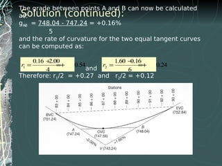
  • 15. The grade between points A and B can now be calculated as: gA-B = 748.04 - 747.24 = +0.16% 5 and the rate of curvature for the two equal tangent curves can be computed as: and Therefore: r1/2 = +0.27 and r2/2 = +0.12 1 0.16 2.0 0.54 4 r + = = + Solution (continued): 1 0.16 2.00 0.54 4 r + = =+ 2 1.60 0.16 0.24 6 r − = =+
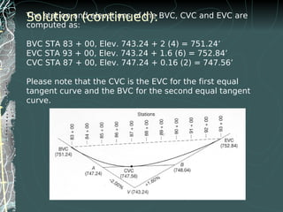
  • 16. The station and elevations of the BVC, CVC and EVC are computed as: BVC STA 83 + 00, Elev. 743.24 + 2 (4) = 751.24’ EVC STA 93 + 00, Elev. 743.24 + 1.6 (6) = 752.84’ CVC STA 87 + 00, Elev. 747.24 + 0.16 (2) = 747.56’ Please note that the CVC is the EVC for the first equal tangent curve and the BVC for the second equal tangent curve. Solution (continued):
  • 17. STATION x g1x (r/2)x 2 CurveElevation BVC 83+00 0 0 0 751.24' 84+00 1 -2.00 85+00 2 86+00 3 CVC 87+00 4 747.56' 88+00 1 0.16 89+00 2 90+00 3 91+00 4 92+00 5 EVC 93+00 6 g1x=-2(1) =-2.00 g2x=.16(1) =0.16 Computation of values for g1x and g2x
  • 18. STATION x g1x (r/2)x 2 CurveElevation BVC 83+00 0 0 0 751.24' 84+00 1 -2.00 0.27 85+00 2 -4.00 86+00 3 -6.00 CVC 87+00 4 -8.00 747.56' 88+00 1 0.16 0.12 89+00 2 0.32 90+00 3 0.48 91+00 4 0.64 92+00 5 0.80 EVC 93+00 6 0.96 (r1/2)x 2 =(0.27)(1) 2 =0.27 (r2/2)x 2 =(0.12)(1) 2 =0.12 Computation of values for (r1/2)x2 and (r2/2)x2
  • 19. STATION x g1x (r/2)x 2 CurveElevation BVC 83+00 0 0 0 751.24' 84+00 1 -2.00 0.27 85+00 2 -4.00 1.08 86+00 3 -6.00 2.43 CVC 87+00 4 -8.00 4.32 747.56' 88+00 1 0.16 0.12 89+00 2 0.32 0.48 90+00 3 0.48 1.08 91+00 4 0.64 1.92 92+00 5 0.80 3.00 EVC 93+00 6 0.96 4.32 Y1 =751.24-2.00+0.27=749.51' Y2 =747.56+0.16+0.12=747.84' Elevation Computations for both Vertical Curves
  • 20. STATION x g1x (r/2)x 2 CurveElevation BVC 83+00 0 0 0 751.24' 84+00 1 -2.00 0.27 749.51' 85+00 2 -4.00 1.08 748.32' 86+00 3 -6.00 2.43 747.67' CVC 87+00 4 -8.00 4.32 747.56' 88+00 1 0.16 0.12 747.84' 89+00 2 0.32 0.48 748.36' 90+00 3 0.48 1.08 749.12' 91+00 4 0.64 1.92 750.12 92+00 5 0.80 3.00 751.36' EVC 93+00 6 0.96 4.32 752.84' Computed Elevations for Stakeout at Full Stations (OK)
  • 21. Designing a Curve to Pass Through a Fixed Point Design a equal-tangent vertical curve to meet a railroad crossing which exists at STA 53 + 50 and elevation 1271.20’. The back grade of -4% meets the forward grade of +3.8% at PVI STA 52 + 00 with elevation 1261.50.
  • 22. Solution: 2 1 2 1 1 2 2 (5350 5200) 150' 1.5 2 2 2 2 1261.50 4.00 2 4.00 4.00 1.5 2 3.80 4.00 3.80 4.00 1.5 2 2 2 BVC BVC L L L x stations r y y g x x g g r L L Y L g x x r L r L x L = + − = + = + = + + − =   = +       = − = − +    + = +   = +   
  • 23. Solution (continued): 2 2 2 3.80 4.00 1271.20 1261.50 4.00 4.00 1.5 1.5 2 2 2 2 0.975 9.85 8.775 0 4 2 0.975 9.85 8.775 9.1152 911.52' L L L L L L b b ac x a a b c L stations      +      = + + − + + +                      − + = − ± − = = = − = = = Check by substituting x = [(9.1152/2)+1.5] stations into the elevation equation to see if it matches a value of 1271.20’
  • 24. Sight Distance Defined as “the distance required, for a given design speed to safely stop a vehicle thus avoiding a collision with an unexpected stationary object in the roadway ahead” by AASHTO (American Association of State Highway and Transportation Officials) Types Stopping Sight Distance Passing Sight Distance Decision Sight Distance Horizontal Sight Distance
  • 25. Sight Distance Equations For Crest Curves For Sag Curves ( ) ( ) ( ) 2 1 2 1 2 2 1 2 1 2 2 2 2 S L S g g L h h S L h h L S g g ≤ − = + ≥ + = − − ( )2 2 1 1 2 4 3.5 4 3.5 2 S L S g g L S S L S L S g g ≤ − = + ≥ + = − − h1: height of the driver’s eye above the roadway h2: height of an object sighted on the roadway AASHTO recommendations: h1 = 3.5 ft, h2 = 0.50 ft (stopping), h2 = 4.25 ft (passing) Lengths of sag vertical curves are based upon headlight criteria for nighttime driving conditions.