SlideShare a Scribd company logo
Bayesian Neural Network
Natan Katz
Natan.katz@gmail.com
Agenda
• Short Introduction to Bayesian Inference
• Variational Inference
• Bayesian Neural Network
• Numerical Methods
• MNIST Example
Bayesian Inference
Bayesian Inference
The inputs:
Evidence – A Sample of observations (numbers, categories, vectors, images)
Hypothesis - An assumption about the prob. structure that creates the sample
Objective :
We wish to learn the optimal parameters of this distribution.
• This probability is called Posterior .
• We wish to find the optimal parameters for P(H|E)
• Remark In many books it is called MAP (Maximum A postriori Estimation)
Let’s Formulate
Z- R.V. that represents the hypothesis
X- R.V. that represents the evidence
Bayes formula:
P(Z|X) =
𝑃(𝑍,𝑋)
𝑃(𝑋)
Let’s Formulate (Cont.)
𝑃𝑟(Z) –Prior (The parameters’ distribution according to our belief)
𝑃𝑙(X|Z) –Likelihood (How likely is the sample given the parameters)
P(Z|X) =
𝑃𝑟(z) 𝑃 𝑙(x|z)
𝑃(𝑋)
Bayesian inference is therefore about working with the RHS terms.
In some case studying the denominator is intractable or extremely
difficult to calculate.
Example -GMM
We have K Gaussians with known variance σ
Draw μ 𝑘 ~ 𝑁 0, τ (τ is positive) from the prior
For each sample j =1…n
𝑧𝑗 ~Cat (1/K,1/K…1/K)
𝑥𝑗 ~ 𝑁(μ 𝑧 𝑗
, σ)
p(𝑥1….𝑛) = μ1:𝑘 𝑙=1
𝐾
𝑃(μ𝑙) 𝑖=1
𝑛
𝑧 𝑗
𝑝( 𝑧𝑗) P(𝑥𝑖|μ 𝑧 𝑗
) => 𝑃𝑟𝑒𝑡𝑡𝑦 𝑆ℎ𝑖𝑡
Some Good news
P(Z|X) =
𝑃𝑟(z) 𝑃 𝑙(x|z)
𝑃(𝑋)
• We wish to learn Z
• There is no Z in the denominator
=> P(Z|X) α 𝑃𝑙 𝑋 𝑍 𝑃𝑟(𝑍)
Solutions
Until 1999
Mostly numerical sampling:
• Metropolis Hastings
• RBM
Variational
Inference
“AN INTRODUCTION TO VARIATIONAL METHODS FOR GRAPHICAL MODELS”
11
VI – Algorithm Overview
• Rather a numerical sampling method we provide an analytical one:
1. We define a distribution family Q(Z) (bias-variance trade off)
2. We minimize KL divergence min KL(Q(z)|| P(Z|X))
log(P(X)) = 𝐸 𝑄 [log P(x, Z)] − 𝐸 𝑄 [log Q(Z)] + KL(Q(Z)||P(Z|X))
ELBO-Evidence Lower Bound
• Maximizing ELBO =>minimizing KL
𝐸𝐿𝐵𝑂 = 𝐸 𝑄[log P(X, Z)] − 𝐸 𝑄 [log Q(Z)] = 𝑄𝐿𝑜𝑔(
𝑃(𝑋,𝑍)
𝑄(𝑍)
)= J(Q)- Euler Lagrange
MFT (Mean Field Theory)
Scientific “approval”
13
What Deep Learning
doesn’t do
A DL Scenario
• We train a CNN to identify images (men versus women)
• Our accuracy can be amazing (98-99%)
Pretty cool
Let’s get Cruel
• We offer the model an image of a basketball
• The model outputs “man” or “woman”
Why is that?
Mathematical Observation
We trained a function F such that
F : {space of images}->{“man”,”woman”}
Statistical Observation
Basketball image is out of our training data
Anecdotes
Image (Uri Itay)
• Researchers trained a network to classify tanks and trees.
After using 200 images (100 of each kind 50 train 50 test), the test accuracy
was 100% .
As they took it to the Pentagon it began to miss. The reason was that all the
tank images were taken in cloudy days whereas trees in sunny.
Text
• We can see in text problems many cases where rather finding latent
phenomena networks use words as their anchor.
A plausible corollary
When we train a DL model:
• We hardly ever know what the model learned
• Models cannot “report” about their uncertainties
Is it crucial ?
• Consider an engine that decides upon AI whether a tumor is
malignant or benign
• Drug treatment upon medical record
• Actions that are taken by an autonomous vehicle
• High frequency trading
What can we do?
• DL models are trained to the optimal weights
• What if rather training weights pointwise, we ill train
weights’ distributions?
The Inference
• For each data pair (x,y) we create mean and variance
• This variance will reflect model’s uncertainty
• DL approach – Do Dropout in inference
Uncertainty Types
Epistemic Uncertainty :
Episteme= Knowledge
Uncertainty that theoretically we can know but we don’t:
• Model structure issues
• Absence of data
We can use the notion “reducible” too
Uncertainty Types
Aleatoric Uncertainty :
Aleator = Dice Player
Uncertainty that we cannot solve:
• The stochasticity of a dice
• Noisy labels
We can use the notion “irreducible” too
Bayesian Neural Network
BNN-Training
• We have a neural network
• We place a prior distribution P over the weights W
• For data D={ (X,Y)}
For measuring uncertainties, we use the posterior Distribution
DL Vs. BNN
DL
1. Training using a loss that is related to prediction probability P(Y|X,W)
2. The weights W are trained point-wise with MLE
Bayesian NN
1. Training using a loss that is related the posterior probability P(W|X,Y)
2. We train weights’ distribution
BNN-Inference
Inference
We assume prior knowledge on the weights’ distribution π
As in any NN we get an input x’ and aim to predict y’ :
P(y’| x’) = 𝑃 y’ 𝑥′
, 𝑤 𝑃 𝑤 𝐷 𝑑𝑤
This can be rewritten as:
P(y’| x’) =𝐸 𝑃(𝑤|𝐷) 𝑃 y’ 𝑥′
, 𝑤
D={(X,Y)}
Measuring Uncertainty
• In the inference, given a data point 𝑥∗
• Sample weights W 𝑛 𝑡𝑖𝑚𝑒𝑠
• Calculate its statistics
E[f(𝑥∗
,w)]= 𝑖=1
𝑛
𝑓(𝑥∗
, 𝑤𝑖)
V([f(𝑥∗
,w)] =E𝑓(𝑥∗
,w)2
- E[f(𝑥∗
,w)]2
W –r.v. which 𝑤𝑖 is its samples
Common tools to obtain Posterior Dist.
1. Variational Inference
2. MCMC –Sampling (Metropolis –Hastings, Gibbs)
3. HMC
4. SGLD
Metropolis Hastings
• MCMC sampling algorithm
• The main idea is that we pick samples upon pdf comparisons:
At each step we accept or randomize a sample upon the previous
sample and decide to accept or reject
• Unbiased, Huge variance and very slow (iterate over the entire data)
• Great History
Bayesian Neural Networks
What is Hamiltonian?
• A physical operator that measures energy of a dynamical system
Two sets of coordinates
q -State coordinates
p- Momentum
H(p, q) =U(q) +K(p)
U(q) = log[π 𝑞 𝐿(𝑞|𝐷)] K(P)=
𝑝 2
2𝑚
U-Potential energy, K –Kinetic
𝑑𝐻
𝑑𝑝
= 𝑞 ,
𝑑𝐻
𝑑𝑞
= - 𝑝
Hamiltonian Monte Carlo
• Hamiltonians offer a deterministic vector field (with trajectories….)
• If we set a Hamiltonian depended distribution, we can use this
property for sampling
P(x,y) = 𝑒−𝐻(𝑥,𝑦)
Hybrid - MC
• We have the “state space” x
• We can add “momentum” and use Hamiltonian mechanism
Leap Frog Algorithm
We set a time interval δ, For each step i :
1. 𝑃𝑖(t+0.5 δ) =𝑃𝑖(t) – (δ/2)
𝑑𝑈
𝑑𝑞(𝑡)
2 𝑄𝑖(t+ δ ) = 𝑄𝑖(t) + δ
𝑑𝐾
𝑑𝑝(𝑡+0.5δ)
3 𝑃𝑖(t+ δ) = 𝑃𝑖(t+0.5 δ) - (δ/2)
𝑑𝑈
𝑑𝑞(𝑡+δ)
𝑄𝑖
𝑄
HMC
Algorithm (Neal 1995, 2012, Duane 1987)
1. Draw 𝑥0 from our prior
Draw 𝑝0 from standard normal dist.
2. Perform L steps of leapfrog
3 Pick the 𝑥 𝑡 following M.H.
Bayesian Neural Networks
HMC –Pros & Cons
Pros
• It takes points from a wider domains thus we can describe the
distribution better
• It may take points with lower density
• Faster than MCMC
Cons
• It may suffer from low energy barrier
• No minibatch –Not nice
• It has to calculate gradients for the entire data!!! Bad
What do we need then?
• A tool that allows sub-sampling
• Fewer Gradients
• Keen knowledge about extremums and escape rooms
Stochastic Gradient
Langevin Dynamics
(SGLD)
Langevin Equation
Langevin Equation describes the motion of pollen grain in water:
F -γ𝑣 𝑡 +ξ 𝑡=0 ξ 𝑡 ~N(0,t)
ξ 𝑡 is a Brownian Force- The collisions with the water molecules
F - External forces
This equation has an equilibrium solution which is our posterior
distribution
Langevin Equation
Let’s use the following:
F=𝛻𝐸 𝑣 𝑡 =
𝑑𝑋
𝑑𝑇
The eq in its discrete form becomes:
𝑥𝑡+1 = 𝑥𝑡 +
dt
γ
ξ 𝑡 + 𝛻𝐸
dt
γ
(looks familiar doesn’t it?)
Langevin Equation
Some more re-write:
𝑥𝑡+1 = 𝑥𝑡 + 𝜖 𝑡 𝛻𝐸 +ε 𝑡 ε 𝑡 -Stochastic term
Consider this term
Are we in a better situation ?
Robbins & Monro (Stoch. Approx. 1951)
• Let F a function and θ a number
• There exists a unique solution :
F(𝑥∗ ) = θ
F - is unknown
Y - A measurable r.v.
E[Y(x)] = F(x)
Robbins &
Monro
(cont)
The following algorithm converges to 𝑥∗ :
𝑋 𝑁+1 = 𝑋 𝑁 +α 𝑁 (𝑌𝑁 − θ )
Back to Langevin
𝑥 𝑡+1 = 𝑥 𝑡 + 𝜖 𝑡 𝛻𝐸 +ε 𝑡
𝛻𝐸 𝑚𝑏=𝛻𝐸 + ε 𝑡
𝑥 𝑡+1 = 𝑥 𝑡 + 𝜖 𝑡 𝛻𝐸 𝑚𝑏
Δ 𝜃𝑡 =ε 𝑡(𝛻log 𝑝 𝜃𝑡 +
𝑁
𝑛 𝑖=1
𝑁
𝛻log 𝑝 𝑥𝑖|𝜃𝑡 )
We are almost there
• This eq converges to an optimal solution (MAP).
• We need a solution of SDE (probability)
• Let’s add a stochastic term
Δ 𝜃𝑡 =ε 𝑡(𝛻log 𝑝 𝜃𝑡 +
𝑁
𝑛 𝑖=1
𝑁
𝛻log 𝑝 𝑥𝑖|𝜃𝑡 ) + η 𝑡 η 𝑡~N(0,σ)
Variance Analysis
ε 𝑡 - Follow R&M rules
How big is σ ?
Bigger than ε 𝑡 *V(𝛻)
As t->∞ the equation must become Langevin.
THE variance of η must be therefore bigger than ε 𝑡 *V(𝛻)
We do the
following:
Finally, Example
https://towardsdatascience.com/making-your-neural-network-say-i-
dont-know-bayesian-nns-using-pyro-and-pytorch-b1c24e6ab8cd
Problem’s Framework
• MNIST CNN model
• MNIST SOTA ~99.8%
The Experiment
• Training a BNN – using VI (small amount, of epochs)
• Set a regular decision law – Take the max score of each digit
=>Accuracy ~88%
Allowing the Network to refuse
• For each image:
• Sample 100 networks
• We obtain 100 outputs per image
• We have 10 digits each with 100 scores
• If the median of these 100 scores>0.2 we take
(Indeed, we can accept more than one result)
Bayesian Neural Networks
Random Image
Summary
• Accuracy 96%
• Refuse 12.5%
• Random images 95% have been refused
Thanks!!
My process
• https://wjmaddox.github.io/assets/BNN_tutorial_CILVR.pdf
• https://arxiv.org/pdf/2007.06823.pdf
• https://towardsdatascience.com/what-uncertainties-tell-you-in-bayesian-neural-networks-6fbd5f85648e
• https://medium.com/@uriitai/augmentation-and-groups-theory-795c287fec3f
• https://github.com/paraschopra/bayesian-neural-network-mnist/blob/master/bnn.ipynb
• https://towardsdatascience.com/making-your-neural-network-say-i-dont-know-bayesian-nns-using-pyro-
and-pytorch-b1c24e6ab8cd
• http://www.stats.ox.ac.uk/~teh/research/compstats/WelTeh2011a.pdf
• https://arxiv.org/pdf/1206.1901.pdf
• http://cgl.elte.hu/~racz/Stoch-diff-eq.pdf
• https://arxiv.org/ftp/arxiv/papers/1103/1103.1184.pdf
• https://henripal.github.io/blog/langevin
• https://www.cs.princeton.edu/courses/archive/fall11/cos597C/lectures/variational-inference-i.pdf

More Related Content

PDF
Bayesian inference
PDF
Naive Bayes
PPTX
Logistic Regression | Logistic Regression In Python | Machine Learning Algori...
PDF
Methods of Optimization in Machine Learning
ODP
Introduction to Principle Component Analysis
PDF
Unified Approach to Interpret Machine Learning Model: SHAP + LIME
PDF
Latent Dirichlet Allocation
PPTX
Feature Selection in Machine Learning
Bayesian inference
Naive Bayes
Logistic Regression | Logistic Regression In Python | Machine Learning Algori...
Methods of Optimization in Machine Learning
Introduction to Principle Component Analysis
Unified Approach to Interpret Machine Learning Model: SHAP + LIME
Latent Dirichlet Allocation
Feature Selection in Machine Learning

What's hot (20)

PDF
Linear models for classification
PPTX
Support vector machine
PPTX
Hyperparameter Tuning
ODP
Introduction to Bayesian Statistics
PDF
Linear regression
PPT
Bayes Classification
ODP
Machine Learning With Logistic Regression
PDF
Bias and variance trade off
PPTX
Support Vector Machine ppt presentation
PPTX
Support vector machine
PPTX
Perceptron & Neural Networks
PDF
Introduction to XGBoost
PPTX
Unsupervised learning (clustering)
PPTX
Machine Learning Tutorial Part - 1 | Machine Learning Tutorial For Beginners ...
PDF
Dimensionality Reduction
PPTX
Lecture 18: Gaussian Mixture Models and Expectation Maximization
PDF
Tuning learning rate
PPTX
PPSX
Lasso and ridge regression
PDF
Classification
Linear models for classification
Support vector machine
Hyperparameter Tuning
Introduction to Bayesian Statistics
Linear regression
Bayes Classification
Machine Learning With Logistic Regression
Bias and variance trade off
Support Vector Machine ppt presentation
Support vector machine
Perceptron & Neural Networks
Introduction to XGBoost
Unsupervised learning (clustering)
Machine Learning Tutorial Part - 1 | Machine Learning Tutorial For Beginners ...
Dimensionality Reduction
Lecture 18: Gaussian Mixture Models and Expectation Maximization
Tuning learning rate
Lasso and ridge regression
Classification
Ad

Similar to Bayesian Neural Networks (20)

PPTX
GAN for Bayesian Inference objectives
PPTX
SGLD Berlin ML GROUP
PDF
Bayesian Deep Learning
PPTX
Deep generative learning_icml_part1
PDF
Deep VI with_beta_likelihood
PDF
Variational inference
PDF
ベイジアンディープニューラルネット
PDF
Modeling uncertainty in deep learning
PPTX
Machine Learning Algorithms Review(Part 2)
PDF
Introduction to modern Variational Inference.
PDF
Deep Learning in Finance
PPTX
Into to prob_prog_hari (2)
PPTX
NICE Implementations of Variational Inference
PPTX
NICE Research -Variational inference project
PDF
Uncertainty in deep learning
PPTX
Deep learning from a novice perspective
PDF
Uncertainty in Deep Learning
PDF
Probabilistic AI Lecture 1: Introduction to variational inference and the ELBO
PDF
QMC Program: Trends and Advances in Monte Carlo Sampling Algorithms Workshop,...
PDF
is anyone_interest_in_auto-encoding_variational-bayes
GAN for Bayesian Inference objectives
SGLD Berlin ML GROUP
Bayesian Deep Learning
Deep generative learning_icml_part1
Deep VI with_beta_likelihood
Variational inference
ベイジアンディープニューラルネット
Modeling uncertainty in deep learning
Machine Learning Algorithms Review(Part 2)
Introduction to modern Variational Inference.
Deep Learning in Finance
Into to prob_prog_hari (2)
NICE Implementations of Variational Inference
NICE Research -Variational inference project
Uncertainty in deep learning
Deep learning from a novice perspective
Uncertainty in Deep Learning
Probabilistic AI Lecture 1: Introduction to variational inference and the ELBO
QMC Program: Trends and Advances in Monte Carlo Sampling Algorithms Workshop,...
is anyone_interest_in_auto-encoding_variational-bayes
Ad

More from Natan Katz (14)

PDF
Open Source models security- Supply chain
PDF
AI HIT taught in HIT always believe thanks
PPTX
AI Open-Source Models- Benefits vs. Risks.
PPTX
final_v.pptx
PPTX
AI for PM.pptx
PPTX
Ancestry, Anecdotes & Avanan -DL for Amateurs
PDF
Cyn meetup
PDF
Finalver
PDF
Foundation of KL Divergence
PDF
Quant2a
PPTX
Bismark
PPTX
PDF
Reinfrocement Learning
PPTX
Neural ODE
Open Source models security- Supply chain
AI HIT taught in HIT always believe thanks
AI Open-Source Models- Benefits vs. Risks.
final_v.pptx
AI for PM.pptx
Ancestry, Anecdotes & Avanan -DL for Amateurs
Cyn meetup
Finalver
Foundation of KL Divergence
Quant2a
Bismark
Reinfrocement Learning
Neural ODE

Recently uploaded (20)

PPTX
Introduction to Basics of Ethical Hacking and Penetration Testing -Unit No. 1...
PPTX
IB Computer Science - Internal Assessment.pptx
PPTX
AI Strategy room jwfjksfksfjsjsjsjsjfsjfsj
PPTX
MODULE 8 - DISASTER risk PREPAREDNESS.pptx
PPTX
ALIMENTARY AND BILIARY CONDITIONS 3-1.pptx
PPT
Reliability_Chapter_ presentation 1221.5784
PPTX
Introduction to Firewall Analytics - Interfirewall and Transfirewall.pptx
PPTX
Business Ppt On Nestle.pptx huunnnhhgfvu
PDF
TRAFFIC-MANAGEMENT-AND-ACCIDENT-INVESTIGATION-WITH-DRIVING-PDF-FILE.pdf
PPTX
Business Acumen Training GuidePresentation.pptx
PDF
Fluorescence-microscope_Botany_detailed content
PDF
“Getting Started with Data Analytics Using R – Concepts, Tools & Case Studies”
PDF
Clinical guidelines as a resource for EBP(1).pdf
PDF
.pdf is not working space design for the following data for the following dat...
PPTX
Supervised vs unsupervised machine learning algorithms
PDF
Mega Projects Data Mega Projects Data
PDF
Recruitment and Placement PPT.pdfbjfibjdfbjfobj
PPTX
climate analysis of Dhaka ,Banglades.pptx
PPTX
Introduction to Knowledge Engineering Part 1
PPTX
DISORDERS OF THE LIVER, GALLBLADDER AND PANCREASE (1).pptx
Introduction to Basics of Ethical Hacking and Penetration Testing -Unit No. 1...
IB Computer Science - Internal Assessment.pptx
AI Strategy room jwfjksfksfjsjsjsjsjfsjfsj
MODULE 8 - DISASTER risk PREPAREDNESS.pptx
ALIMENTARY AND BILIARY CONDITIONS 3-1.pptx
Reliability_Chapter_ presentation 1221.5784
Introduction to Firewall Analytics - Interfirewall and Transfirewall.pptx
Business Ppt On Nestle.pptx huunnnhhgfvu
TRAFFIC-MANAGEMENT-AND-ACCIDENT-INVESTIGATION-WITH-DRIVING-PDF-FILE.pdf
Business Acumen Training GuidePresentation.pptx
Fluorescence-microscope_Botany_detailed content
“Getting Started with Data Analytics Using R – Concepts, Tools & Case Studies”
Clinical guidelines as a resource for EBP(1).pdf
.pdf is not working space design for the following data for the following dat...
Supervised vs unsupervised machine learning algorithms
Mega Projects Data Mega Projects Data
Recruitment and Placement PPT.pdfbjfibjdfbjfobj
climate analysis of Dhaka ,Banglades.pptx
Introduction to Knowledge Engineering Part 1
DISORDERS OF THE LIVER, GALLBLADDER AND PANCREASE (1).pptx

Bayesian Neural Networks

  • 1. Bayesian Neural Network Natan Katz Natan.katz@gmail.com
  • 2. Agenda • Short Introduction to Bayesian Inference • Variational Inference • Bayesian Neural Network • Numerical Methods • MNIST Example
  • 4. Bayesian Inference The inputs: Evidence – A Sample of observations (numbers, categories, vectors, images) Hypothesis - An assumption about the prob. structure that creates the sample Objective : We wish to learn the optimal parameters of this distribution. • This probability is called Posterior . • We wish to find the optimal parameters for P(H|E) • Remark In many books it is called MAP (Maximum A postriori Estimation)
  • 5. Let’s Formulate Z- R.V. that represents the hypothesis X- R.V. that represents the evidence Bayes formula: P(Z|X) = 𝑃(𝑍,𝑋) 𝑃(𝑋)
  • 6. Let’s Formulate (Cont.) 𝑃𝑟(Z) –Prior (The parameters’ distribution according to our belief) 𝑃𝑙(X|Z) –Likelihood (How likely is the sample given the parameters) P(Z|X) = 𝑃𝑟(z) 𝑃 𝑙(x|z) 𝑃(𝑋) Bayesian inference is therefore about working with the RHS terms. In some case studying the denominator is intractable or extremely difficult to calculate.
  • 7. Example -GMM We have K Gaussians with known variance σ Draw μ 𝑘 ~ 𝑁 0, τ (τ is positive) from the prior For each sample j =1…n 𝑧𝑗 ~Cat (1/K,1/K…1/K) 𝑥𝑗 ~ 𝑁(μ 𝑧 𝑗 , σ) p(𝑥1….𝑛) = μ1:𝑘 𝑙=1 𝐾 𝑃(μ𝑙) 𝑖=1 𝑛 𝑧 𝑗 𝑝( 𝑧𝑗) P(𝑥𝑖|μ 𝑧 𝑗 ) => 𝑃𝑟𝑒𝑡𝑡𝑦 𝑆ℎ𝑖𝑡
  • 8. Some Good news P(Z|X) = 𝑃𝑟(z) 𝑃 𝑙(x|z) 𝑃(𝑋) • We wish to learn Z • There is no Z in the denominator => P(Z|X) α 𝑃𝑙 𝑋 𝑍 𝑃𝑟(𝑍)
  • 9. Solutions Until 1999 Mostly numerical sampling: • Metropolis Hastings • RBM
  • 11. “AN INTRODUCTION TO VARIATIONAL METHODS FOR GRAPHICAL MODELS” 11
  • 12. VI – Algorithm Overview • Rather a numerical sampling method we provide an analytical one: 1. We define a distribution family Q(Z) (bias-variance trade off) 2. We minimize KL divergence min KL(Q(z)|| P(Z|X)) log(P(X)) = 𝐸 𝑄 [log P(x, Z)] − 𝐸 𝑄 [log Q(Z)] + KL(Q(Z)||P(Z|X)) ELBO-Evidence Lower Bound • Maximizing ELBO =>minimizing KL
  • 13. 𝐸𝐿𝐵𝑂 = 𝐸 𝑄[log P(X, Z)] − 𝐸 𝑄 [log Q(Z)] = 𝑄𝐿𝑜𝑔( 𝑃(𝑋,𝑍) 𝑄(𝑍) )= J(Q)- Euler Lagrange MFT (Mean Field Theory) Scientific “approval” 13
  • 15. A DL Scenario • We train a CNN to identify images (men versus women) • Our accuracy can be amazing (98-99%) Pretty cool
  • 16. Let’s get Cruel • We offer the model an image of a basketball • The model outputs “man” or “woman”
  • 17. Why is that? Mathematical Observation We trained a function F such that F : {space of images}->{“man”,”woman”} Statistical Observation Basketball image is out of our training data
  • 18. Anecdotes Image (Uri Itay) • Researchers trained a network to classify tanks and trees. After using 200 images (100 of each kind 50 train 50 test), the test accuracy was 100% . As they took it to the Pentagon it began to miss. The reason was that all the tank images were taken in cloudy days whereas trees in sunny. Text • We can see in text problems many cases where rather finding latent phenomena networks use words as their anchor.
  • 19. A plausible corollary When we train a DL model: • We hardly ever know what the model learned • Models cannot “report” about their uncertainties
  • 20. Is it crucial ? • Consider an engine that decides upon AI whether a tumor is malignant or benign • Drug treatment upon medical record • Actions that are taken by an autonomous vehicle • High frequency trading
  • 21. What can we do? • DL models are trained to the optimal weights • What if rather training weights pointwise, we ill train weights’ distributions? The Inference • For each data pair (x,y) we create mean and variance • This variance will reflect model’s uncertainty • DL approach – Do Dropout in inference
  • 22. Uncertainty Types Epistemic Uncertainty : Episteme= Knowledge Uncertainty that theoretically we can know but we don’t: • Model structure issues • Absence of data We can use the notion “reducible” too
  • 23. Uncertainty Types Aleatoric Uncertainty : Aleator = Dice Player Uncertainty that we cannot solve: • The stochasticity of a dice • Noisy labels We can use the notion “irreducible” too
  • 25. BNN-Training • We have a neural network • We place a prior distribution P over the weights W • For data D={ (X,Y)} For measuring uncertainties, we use the posterior Distribution
  • 26. DL Vs. BNN DL 1. Training using a loss that is related to prediction probability P(Y|X,W) 2. The weights W are trained point-wise with MLE Bayesian NN 1. Training using a loss that is related the posterior probability P(W|X,Y) 2. We train weights’ distribution
  • 27. BNN-Inference Inference We assume prior knowledge on the weights’ distribution π As in any NN we get an input x’ and aim to predict y’ : P(y’| x’) = 𝑃 y’ 𝑥′ , 𝑤 𝑃 𝑤 𝐷 𝑑𝑤 This can be rewritten as: P(y’| x’) =𝐸 𝑃(𝑤|𝐷) 𝑃 y’ 𝑥′ , 𝑤 D={(X,Y)}
  • 28. Measuring Uncertainty • In the inference, given a data point 𝑥∗ • Sample weights W 𝑛 𝑡𝑖𝑚𝑒𝑠 • Calculate its statistics E[f(𝑥∗ ,w)]= 𝑖=1 𝑛 𝑓(𝑥∗ , 𝑤𝑖) V([f(𝑥∗ ,w)] =E𝑓(𝑥∗ ,w)2 - E[f(𝑥∗ ,w)]2 W –r.v. which 𝑤𝑖 is its samples
  • 29. Common tools to obtain Posterior Dist. 1. Variational Inference 2. MCMC –Sampling (Metropolis –Hastings, Gibbs) 3. HMC 4. SGLD
  • 30. Metropolis Hastings • MCMC sampling algorithm • The main idea is that we pick samples upon pdf comparisons: At each step we accept or randomize a sample upon the previous sample and decide to accept or reject • Unbiased, Huge variance and very slow (iterate over the entire data) • Great History
  • 32. What is Hamiltonian? • A physical operator that measures energy of a dynamical system Two sets of coordinates q -State coordinates p- Momentum H(p, q) =U(q) +K(p) U(q) = log[π 𝑞 𝐿(𝑞|𝐷)] K(P)= 𝑝 2 2𝑚 U-Potential energy, K –Kinetic 𝑑𝐻 𝑑𝑝 = 𝑞 , 𝑑𝐻 𝑑𝑞 = - 𝑝
  • 33. Hamiltonian Monte Carlo • Hamiltonians offer a deterministic vector field (with trajectories….) • If we set a Hamiltonian depended distribution, we can use this property for sampling P(x,y) = 𝑒−𝐻(𝑥,𝑦)
  • 34. Hybrid - MC • We have the “state space” x • We can add “momentum” and use Hamiltonian mechanism Leap Frog Algorithm We set a time interval δ, For each step i : 1. 𝑃𝑖(t+0.5 δ) =𝑃𝑖(t) – (δ/2) 𝑑𝑈 𝑑𝑞(𝑡) 2 𝑄𝑖(t+ δ ) = 𝑄𝑖(t) + δ 𝑑𝐾 𝑑𝑝(𝑡+0.5δ) 3 𝑃𝑖(t+ δ) = 𝑃𝑖(t+0.5 δ) - (δ/2) 𝑑𝑈 𝑑𝑞(𝑡+δ) 𝑄𝑖 𝑄
  • 35. HMC Algorithm (Neal 1995, 2012, Duane 1987) 1. Draw 𝑥0 from our prior Draw 𝑝0 from standard normal dist. 2. Perform L steps of leapfrog 3 Pick the 𝑥 𝑡 following M.H.
  • 37. HMC –Pros & Cons Pros • It takes points from a wider domains thus we can describe the distribution better • It may take points with lower density • Faster than MCMC Cons • It may suffer from low energy barrier • No minibatch –Not nice • It has to calculate gradients for the entire data!!! Bad
  • 38. What do we need then? • A tool that allows sub-sampling • Fewer Gradients • Keen knowledge about extremums and escape rooms
  • 40. Langevin Equation Langevin Equation describes the motion of pollen grain in water: F -γ𝑣 𝑡 +ξ 𝑡=0 ξ 𝑡 ~N(0,t) ξ 𝑡 is a Brownian Force- The collisions with the water molecules F - External forces This equation has an equilibrium solution which is our posterior distribution
  • 41. Langevin Equation Let’s use the following: F=𝛻𝐸 𝑣 𝑡 = 𝑑𝑋 𝑑𝑇 The eq in its discrete form becomes: 𝑥𝑡+1 = 𝑥𝑡 + dt γ ξ 𝑡 + 𝛻𝐸 dt γ (looks familiar doesn’t it?)
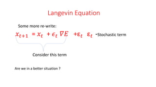
  • 42. Langevin Equation Some more re-write: 𝑥𝑡+1 = 𝑥𝑡 + 𝜖 𝑡 𝛻𝐸 +ε 𝑡 ε 𝑡 -Stochastic term Consider this term Are we in a better situation ?
  • 43. Robbins & Monro (Stoch. Approx. 1951) • Let F a function and θ a number • There exists a unique solution : F(𝑥∗ ) = θ F - is unknown Y - A measurable r.v. E[Y(x)] = F(x)
  • 44. Robbins & Monro (cont) The following algorithm converges to 𝑥∗ : 𝑋 𝑁+1 = 𝑋 𝑁 +α 𝑁 (𝑌𝑁 − θ )
  • 45. Back to Langevin 𝑥 𝑡+1 = 𝑥 𝑡 + 𝜖 𝑡 𝛻𝐸 +ε 𝑡 𝛻𝐸 𝑚𝑏=𝛻𝐸 + ε 𝑡 𝑥 𝑡+1 = 𝑥 𝑡 + 𝜖 𝑡 𝛻𝐸 𝑚𝑏 Δ 𝜃𝑡 =ε 𝑡(𝛻log 𝑝 𝜃𝑡 + 𝑁 𝑛 𝑖=1 𝑁 𝛻log 𝑝 𝑥𝑖|𝜃𝑡 )
  • 46. We are almost there • This eq converges to an optimal solution (MAP). • We need a solution of SDE (probability) • Let’s add a stochastic term Δ 𝜃𝑡 =ε 𝑡(𝛻log 𝑝 𝜃𝑡 + 𝑁 𝑛 𝑖=1 𝑁 𝛻log 𝑝 𝑥𝑖|𝜃𝑡 ) + η 𝑡 η 𝑡~N(0,σ)
  • 47. Variance Analysis ε 𝑡 - Follow R&M rules How big is σ ? Bigger than ε 𝑡 *V(𝛻) As t->∞ the equation must become Langevin. THE variance of η must be therefore bigger than ε 𝑡 *V(𝛻)
  • 50. Problem’s Framework • MNIST CNN model • MNIST SOTA ~99.8%
  • 51. The Experiment • Training a BNN – using VI (small amount, of epochs) • Set a regular decision law – Take the max score of each digit =>Accuracy ~88%
  • 52. Allowing the Network to refuse • For each image: • Sample 100 networks • We obtain 100 outputs per image • We have 10 digits each with 100 scores • If the median of these 100 scores>0.2 we take (Indeed, we can accept more than one result)
  • 58. Summary • Accuracy 96% • Refuse 12.5% • Random images 95% have been refused
  • 60. My process • https://wjmaddox.github.io/assets/BNN_tutorial_CILVR.pdf • https://arxiv.org/pdf/2007.06823.pdf • https://towardsdatascience.com/what-uncertainties-tell-you-in-bayesian-neural-networks-6fbd5f85648e • https://medium.com/@uriitai/augmentation-and-groups-theory-795c287fec3f • https://github.com/paraschopra/bayesian-neural-network-mnist/blob/master/bnn.ipynb • https://towardsdatascience.com/making-your-neural-network-say-i-dont-know-bayesian-nns-using-pyro- and-pytorch-b1c24e6ab8cd • http://www.stats.ox.ac.uk/~teh/research/compstats/WelTeh2011a.pdf • https://arxiv.org/pdf/1206.1901.pdf • http://cgl.elte.hu/~racz/Stoch-diff-eq.pdf • https://arxiv.org/ftp/arxiv/papers/1103/1103.1184.pdf • https://henripal.github.io/blog/langevin • https://www.cs.princeton.edu/courses/archive/fall11/cos597C/lectures/variational-inference-i.pdf